School of Applied Sciences Department of Electronics...
58
TECHNOLOGICAL EDUCATIONAL INSTITUTE OF CRETE School of Applied Sciences Department of Electronics Engineering Dissertation Robust Object Recognition in Digital Images Evangelos Kandounakis Supervisor Professor Dr. Emmanouil Skounakis, MSc, MSc. June 2014
Transcript of School of Applied Sciences Department of Electronics...
TECHNOLOGICAL EDUCATIONAL INSTITUTE OF CRETE
School of Applied Sciences
Department of Electronics Engineering
Dissertation
Robust Object Recognition in Digital Images
Evangelos Kandounakis
Supervisor Professor Dr. Emmanouil Skounakis, MSc, MSc.
June 2014

2

3
To Mum, Dad and Sister

4
Abstract
Nowadays, image processing is a very challenging task due to the fact that digital technology
finds more and more applications. This dissertation presents an interactive environment
that allows the automatic human-computer communication with applications in visual
control of multimedia data.

5
Acknowledgements
I would like to express my gratitude to my supervisor professor, Dr. Emmanouil Skounakis,
for offering his constant support, invaluable comments on my work, and continuing regard
and guidance throughout this dissertation.
He has been influential in my choice of image processing as my field of study. His academic
knowledge and advice have been essential to the completion of this dissertation.
I would also like to thank my parents, John and Stephanie, and my sister for their love and
support throughout my studies.
6
Table of Contents
Abstract ………………………………………………………………………… 4
Acknowledgements ………………………………………………………. 5
Table of Contents ………………………………………………………….. 6
Chapter 1 Introduction ………………………………………………………………….. 8
1.1 Light ………………………………………………………………………………… 21
1.1.1 The Electromagnetic Spectrum …………………………… 21
1.1.2 Dispersion of light ……………………………………………….. 21
1.2 Digital Images ………………………………………………………………….. 22
1.3 Human Vision ………………………………………………………………….. 25
1.3.1 The Human Eye Structure ……………………………………. 25
1.3.2 Retina …………………………………………………………………. 26
1.3.3 From Eye to Brain ……………………………………………….. 27
1.3.4 Two Visual Paths …………………………………………………. 28
1.4 Digital Image Algebraic Operations ………………………………….
………………………………….......
29
1.4.1 Arithmetic Operations ………………………………………… 29
1.4.2 Logical Operations ………………………………………………. 30
1.4.3 Operations between Matrices …………………………….. 31
1.5 Digital Image Geometric Operations ……………………………….. 31
1.5.1 Image Rotation ……………………………………………………. 31
1.5.2 Image Flip (Horizontal and Vertical) ……………………. 32
1.6 Digital Image File Formats and Storage ……………………………. 34
1.6.1 Formats of Digital Images ……………………………………. 35
1.7 Color models – Fundamentals …………………………………………. 36
1.7.1 RGB …………………………………………………………………….. 37
1.7.2 CMYK ………………………………………………………………….. 38
1.7.3 HSV (HSB) ……………………………………………………………. 39

7
Chapter 2 Segmentation ……………………………………………………………….. 40
2.1 The Basic Concept …………………………………………………………… 40
2.2 Segmentation Methods and Techniques
…………………………..
40
2.2.1 Thresholding ……………………………………………………….. 40
2.2.2 Sobel Masks ………………………………………………………… 42
2.2.3 Region Growing …………………………………………………… 44
2.2.4 Active Contours …………………………………………………… 48
2.2.5 K-means clustering ……………………………………………… 49
2.2.6 Hough Forests for Object Detection ……………………. 49
Chapter 3 Segmentation Framework …………………………………………….. 52
3.1 Generally ………………………………………………………………………….
3.2 The Proposed Framework for Object Recognition ……………
References ……………………………………………………………………. 56

8
Chapter 1: Introduction
… One picture is worth a thousand words ….
Vision detects the information from the environment which the visible light carries.
It is considered that animals with vision appeared in the Cambrian period and also that the
evolution of a versatility of life forms is associated with it. Moreover, it is claimed that
vision caused serious changes in the morphology of animals as it was associated with several
predatory and defense survival adaptations, such as a hard exoskeleton or even color for
camouflage. [1]
It is known that of all the senses in humans, vision is the most advanced [2]. Actually, vision
is used more than the other senses for carrying out daily activities in the world [3]. Sensing
visible light in the environment and transforming it into action potentials occur in the eye
[4]. However, vision is not located only in the eye. The information from the eyes is
processed in the brain [5]. This processing gives rise to an internal representation of the
environment [3].
Generally, the result of processing sensory information in the brain is perception [6].
Consequently, visual perception is the product of processing visual sensory information in
specialized areas in the brain.
Figure 1.0 – Areas 3 (hidden here), 5, and 7 represent the occipital lobe where the striate and
extrastriate areas are located. The Middle Temporal area is located in where arrow 1 is pointing.
The posterior part (caudal) of the fusiform gyrus (green) contains the FFA for face recognition [7]
9
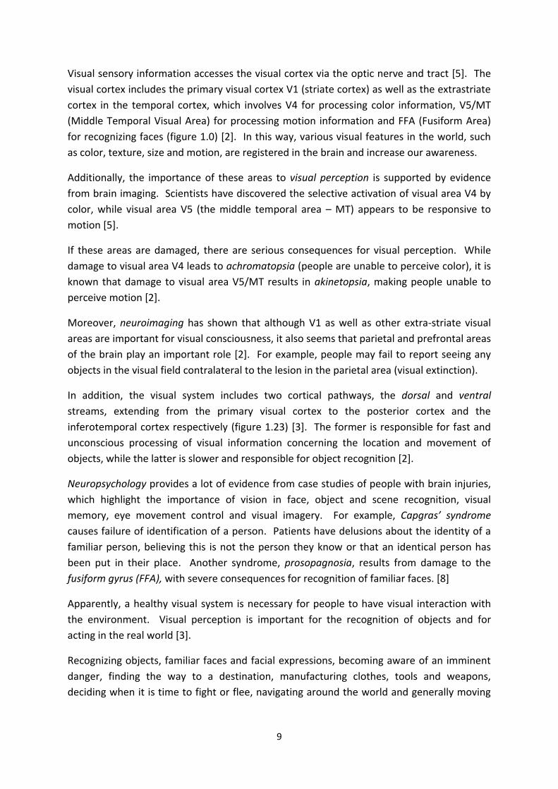
Visual sensory information accesses the visual cortex via the optic nerve and tract [5]. The
visual cortex includes the primary visual cortex V1 (striate cortex) as well as the extrastriate
cortex in the temporal cortex, which involves V4 for processing color information, V5/MT
(Middle Temporal Visual Area) for processing motion information and FFA (Fusiform Area)
for recognizing faces (figure 1.0) [2]. In this way, various visual features in the world, such
as color, texture, size and motion, are registered in the brain and increase our awareness.
Additionally, the importance of these areas to visual perception is supported by evidence
from brain imaging. Scientists have discovered the selective activation of visual area V4 by
color, while visual area V5 (the middle temporal area – MT) appears to be responsive to
motion [5].
If these areas are damaged, there are serious consequences for visual perception. While
damage to visual area V4 leads to achromatopsia (people are unable to perceive color), it is
known that damage to visual area V5/MT results in akinetopsia, making people unable to
perceive motion [2].
Moreover, neuroimaging has shown that although V1 as well as other extra-striate visual
areas are important for visual consciousness, it also seems that parietal and prefrontal areas
of the brain play an important role [2]. For example, people may fail to report seeing any
objects in the visual field contralateral to the lesion in the parietal area (visual extinction).
In addition, the visual system includes two cortical pathways, the dorsal and ventral
streams, extending from the primary visual cortex to the posterior cortex and the
inferotemporal cortex respectively (figure 1.23) [3]. The former is responsible for fast and
unconscious processing of visual information concerning the location and movement of
objects, while the latter is slower and responsible for object recognition [2].
Neuropsychology provides a lot of evidence from case studies of people with brain injuries,
which highlight the importance of vision in face, object and scene recognition, visual
memory, eye movement control and visual imagery. For example, Capgras’ syndrome
causes failure of identification of a person. Patients have delusions about the identity of a
familiar person, believing this is not the person they know or that an identical person has
been put in their place. Another syndrome, prosopagnosia, results from damage to the
fusiform gyrus (FFA), with severe consequences for recognition of familiar faces. [8]
Apparently, a healthy visual system is necessary for people to have visual interaction with
the environment. Visual perception is important for the recognition of objects and for
acting in the real world [3].
Recognizing objects, familiar faces and facial expressions, becoming aware of an imminent
danger, finding the way to a destination, manufacturing clothes, tools and weapons,
deciding when it is time to fight or flee, navigating around the world and generally moving

10
through space, require vision. In other words, a large part of our life is organized around
vision.
However, understanding the importance of vision only within the physiological and
neuropsychological context would limit the perspective. Vision has been important in
human history since the early days of man on Earth.
Unlike other living creatures on our planet, and even among primates, human has the
unique ability to use visual information in order to create representations on the surface of
objects.
Making and using representations of the real world was considered an innate property by
Aristotle in ancient Greece and a human quality, which is expressed through the arts setting
man apart from animals. Representations can describe a variety of ideas and their
expression can take various forms. Consequently, a representation can take the form of a
human or other figure carved on stone or wood , of an image in a painting as well as of
music or words in a written account, all of which could convey various perspectives about
life, for example individual or collective actions, attitudes and values. [9]
In semiotics, representations whose aim is to resemble real objects are categorized as
iconic. One such instance is the case of a painting depicting a human face, a flower or an
animal. Semiotics also identifies symbolic representations, which convey social meanings
about objects in various societies at a given time. For example, the written word ‘airplane’
is the product of the combination of symbols (letters) used in the English language in a
specific way to produce the concept of an manmade object with wings and engines flying in
the sky, a concept familiar to people in the 19th and 20th century. Finally, an indexing
representation is another aspect of a representation which includes intentionality on behalf
of its creator. For example, a carved letter or a drawing on a stone could convey the
intention of one’s presence made known. [9]
Figure 1.1 – Replica of the cave painting of animals originally found in the Chauvet
cave. It dates back to approximately 31,000 BC [10]
11
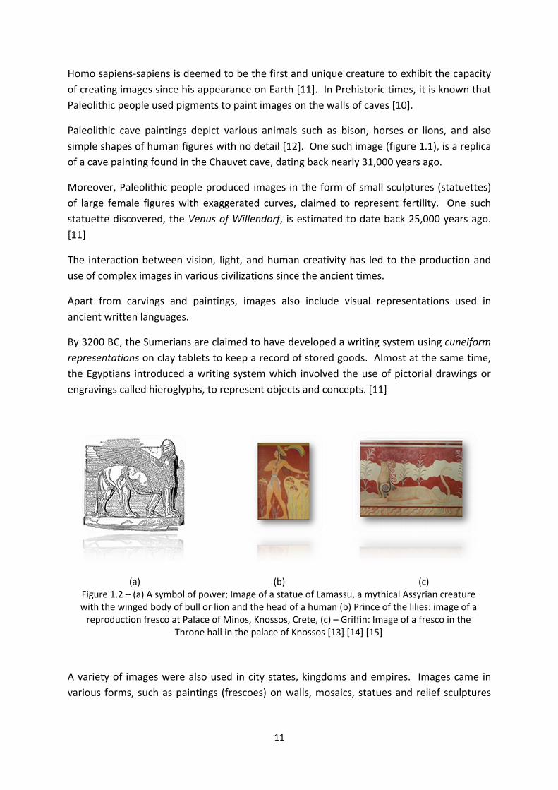
Homo sapiens-sapiens is deemed to be the first and unique creature to exhibit the capacity
of creating images since his appearance on Earth [11]. In Prehistoric times, it is known that
Paleolithic people used pigments to paint images on the walls of caves [10].
Paleolithic cave paintings depict various animals such as bison, horses or lions, and also
simple shapes of human figures with no detail [12]. One such image (figure 1.1), is a replica
of a cave painting found in the Chauvet cave, dating back nearly 31,000 years ago.
Moreover, Paleolithic people produced images in the form of small sculptures (statuettes)
of large female figures with exaggerated curves, claimed to represent fertility. One such
statuette discovered, the Venus of Willendorf, is estimated to date back 25,000 years ago.
[11]
The interaction between vision, light, and human creativity has led to the production and
use of complex images in various civilizations since the ancient times.
Apart from carvings and paintings, images also include visual representations used in
ancient written languages.
By 3200 BC, the Sumerians are claimed to have developed a writing system using cuneiform
representations on clay tablets to keep a record of stored goods. Almost at the same time,
the Egyptians introduced a writing system which involved the use of pictorial drawings or
engravings called hieroglyphs, to represent objects and concepts. [11]
(a) (b) (c) Figure 1.2 – (a) A symbol of power; Image of a statue of Lamassu, a mythical Assyrian creature with the winged body of bull or lion and the head of a human (b) Prince of the lilies: image of a
reproduction fresco at Palace of Minos, Knossos, Crete, (c) – Griffin: Image of a fresco in the Throne hall in the palace of Knossos [13] [14] [15]
A variety of images were also used in city states, kingdoms and empires. Images came in
various forms, such as paintings (frescoes) on walls, mosaics, statues and relief sculptures
12
and included a number of themes ranging from animals, mythical creatures, objects, to
kings and deities. Various image patterns also decorated shields in antiquity [16].
Ancient Assyrians used the Lamassu at the entrance of palaces as guardians and symbols of
power (figure 1.2 (a)). Magnificent frescoes are found in the palace of Minos in Knossos,
Crete, some of which depicted adorned human figures, such as the prince of the lilies (figure
1.2 (b)), while others, such as the ones on the walls of the throne hall, depicted the mythical
creatures griffins, which had the head of an eagle and the body of a lion (figure 1.2 (c)).
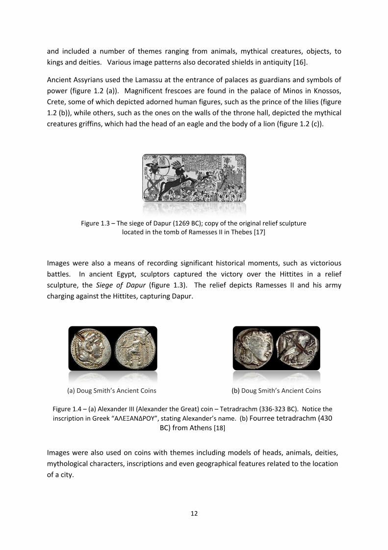
Figure 1.3 – The siege of Dapur (1269 BC); copy of the original relief sculpture
located in the tomb of Ramesses II in Thebes [17]
Images were also a means of recording significant historical moments, such as victorious
battles. In ancient Egypt, sculptors captured the victory over the Hittites in a relief
sculpture, the Siege of Dapur (figure 1.3). The relief depicts Ramesses II and his army
charging against the Hittites, capturing Dapur.
(a) Doug Smith’s Ancient Coins (b) Doug Smith’s Ancient Coins
Figure 1.4 – (a) Alexander III (Alexander the Great) coin – Tetradrachm (336-323 BC). Notice the
inscription in Greek “ΑΛΕΞΑΝΔΡΟΥ”, stating Alexander’s name. (b) Fourree tetradrachm (430 BC) from Athens [18]
Images were also used on coins with themes including models of heads, animals, deities,
mythological characters, inscriptions and even geographical features related to the location
of a city.

13
Images of Hercules wearing a lion skin are found on the one side of the Tetradrachm (336-
323 BC) in figure 1.4 (a), while the other side depicts an image of Zeus seated holding an
eagle and also the inscription ‘ΑΛΕΞΑΝΔΡΟΥ’ in ancient Greek stating Alexander the Great’s
name. Images of Athena and the owl were used on ancient Athenian coins (figure 1.4 (b)
[18]).
Figure 1.5 – Leonardo da Vinci’s Mona Lisa painting [19]
During the Renaissance, a new cultural movement appeared with Latin and Greek classical
influences [19].
Experimentation with light, shadow, color and perspective resulted in numerous images
produced in the form of statues, paintings and murals. One of the most famous works of art
in the Renaissance was the Mona Lisa, painted by Leonardo da Vinci shown in figure 1.5.
Images during that time were also a major influence on the advancement of science. For
example, in medicine, meticulous anatomical representations of the body and organs were
produced in print by Leonardo Da Vinci. There were also architectural images of buildings
(figure 1.6) included in printed books, such as I quattro libri dell'architettura (The four books
of architecture) which was published by Andrea Palladio in Venice, in 1570. [11]
Figure 1.6 – A woodcut of Donato Bramante’s Tempietto in Andrea Palladio’s book
Quattro Libri Dell’Architectura 1570) [20]

14
Human history is teaming with ‘visual products’. Over the last two centuries, great scientific
and technological advances have changed the world of visual images.
The advent of the camera was a revolutionary step that enabled people to capture realistic
images in their environment. The first permanent photographic image was taken, by the
French Joseph Nicéphore Niépce in about 1827, with a camera obscura [21].
Later on, another form of art - the cinema - is considered to have spawned from the
perfection of the Cinematograph, a camera using film to capture motion as well as a film
projector [22].
First evidence of image processing comes from the newspaper industry, in 1920 when they
first used special equipment to transmit photographs via the submarine cable, which
connected the two cities across the Atlantic Ocean, New York and London. First evidence of
the involvement of computers in image processing comes from 1960, when computers
were used to improve of images of the lunar surface sent by Ranger 7 in 1964 (Figure 1.7)
[23].
Figure 1.7 – Courtesy NASA/NSSDC. The US spacecraft Ranger 7 took the first photograph of the
Moon and transmitted it back to Earth, 17 minutes before impact on the lunar surface, on 31st July 1964 at 9:09 AM EDT [24]
The Digital Revolution signified by the transition from analogue to digital technology, led to
the proliferation of a plethora of digital technological advances, which at the end of the 20th
century, included digital monitors, mobile phones, tablets, cameras, computers, fax
machines, photocopying machines and the internet [25].
Especially, the development of computers as well as personal computers with increased
processing power, radically affected the production and generally the manipulation of
images. Actually, computers are involved in Image Processing by means of mathematical
functions to create and manipulate images
In this way, people produce, transmit and generally manipulate images quickly and in large
amounts. Real world Images are captured and transmitted at the click of a button.

15
All these factors made it imperative that new methods and systems should be developed to
handle the huge amount and variety of digital images. Image processing emerged as a new
field of study for the manipulation of images.
It involves processing of visual information contained in images by means of special
algorithms and techniques.
This means that an image is converted into digital data and is introduced into a computer
system for further processing.
Image processing tasks involve processes such as:
Image acquisition and storage
Image pre-processing
Segmentation
Recognition of objects
Image pre-processing is a relatively simpler image processing task compared to
segmentation and recognition of objects processes.
Through the image acquisition process, the main features of the objects contained in an
image are stored in a digital form by means of a camera. In other words, light energy is
turned into digital data. This data is stored in a file, for example image.jpg (as described in
section 1.6.1), in order to be available for viewing or processing.
Different cameras capture an image of an object in different ranges of the electromagnetic
spectrum.
For example, an infrared camera records an image of the invisible infrared radiation that an
object produces or reflects and yields an image of that in the visible spectrum. On the other
hand, an ordinary camera captures the visible radiation that is emitted or reflected by an
object. Some cameras can also provide 2D or 3D images.
Nevertheless, apart from cameras, there is a variety of means which serve as a source of
images, such as Magnetic Resonance Imaging scanners (MRI), Positron Emission
Tomography scanners (PET), Computed Tomography scanners (CT), X-ray devices,
Ultrasound machines and Radars.
The data stored in an image file is introduced into a computer to undergo pre-processing
since the input image should be of satisfying quality to ensure that it meets the criteria
required at the ensuing stages.
For example, during object recognition, matching the features of a candidate object
contained in the input image with the corresponding category features may be unsuccessful,
due to the effect of interfering factors at the preceding stage of acquisition, such as blurring
16
or uneven illumination of an object. Important processes applied at this stage ensure that
the noise is removed or reduced from the image in order to be enhanced partly or wholly.
An interesting idea in image processing is segmentation. Through this process, objects in an
image are delineated. In the real world, objects are not always unambiguously identified
due to factors such as: occlusion, inhomogeneous texture, discontinuity of edges, or uneven
illumination.
Therefore, there is not a unique segmentation method which can be applied successfully to
all cases. Instead, there is a variety of segmentation methods and assistive techniques
which can be selected in different situations to achieve different results.
These include thresholding, Sobel masks, region growing, active contours, K-means
clustering and class-specific Hough Forests.
For example, if the aim is to extract the shape of an object in a simple image, then
segmentation could be achieved using the thresholding technique.
After an image is segmented and identifiable areas are delineated, objects within these
areas need to be recognized. Recognition is not always an easy task for image processing
systems.
While humans can effortlessly and quickly identify boundaries of objects with similar color
representations and recognize a variety of objects even under difficult conditions, it appears
that for computers this task can prove an arduous one.
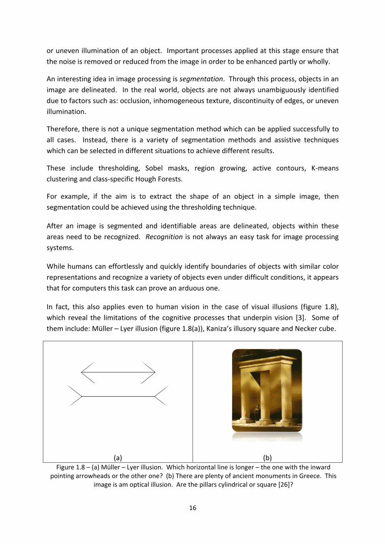
In fact, this also applies even to human vision in the case of visual illusions (figure 1.8),
which reveal the limitations of the cognitive processes that underpin vision [3]. Some of
them include: Müller – Lyer illusion (figure 1.8(a)), Kaniza’s illusory square and Necker cube.
(a)
(b) Figure 1.8 – (a) Müller – Lyer illusion. Which horizontal line is longer – the one with the inward
pointing arrowheads or the other one? (b) There are plenty of ancient monuments in Greece. This image is am optical illusion. Are the pillars cylindrical or square [26]?

17
Image processing has applications in many scientific fields. One major area where image
processing has an important role is the medical field. In medicine, a variety of images is
produced due to the existence of a wide range of imaging modalities for diagnostic
purposes. They allow doctors to examine the internal organs in a patient’s body in a non-
invasive way in order to diagnose potential pathologies and also to track the progress of a
therapy or disease.
Medical image modalities include various types, such as MRI, CT, PET, angiography,
ultrasound and X-ray. Different visualization methods serve different purposes. For
example, the X-ray technology underpinning CT imaging is suitable for images of the bones
contrary to the MRI technology which is more suitable for providing images of soft tissue
[27].
However, medical images are often complex due to the fact that they contain objects whose
boundaries may be blurred. Moreover, low resolution and contrast can also interfere with
the efficiency of visual inspection of medical images and affect extraction of useful medical
information. Medical platforms have been developed, which integrate various image
processing methods, to overcome these problems and increase speed and accuracy of
diagnosis. To this end, methods may involve the enhancement of a medical image,
segmentation of one or more areas of interest in it, recognition of an organ or suspected
pathology, providing metrics and finally 2D or 3D representation of the identified organ (e.g.
kidney) or their pathology (e.g. tumor). [28]
Figure 1.9 – ATD Medical Platform [28]
Biomedical applications also assist research in medicine as they allow the study and
experimentation of new therapeutic approaches.

18
Currently, they allow researchers and physicians to examine the effects of medicines or
surgical approaches with the aim of improving them or discovering new ones.
Nevertheless, the study of extracted information occurs subsequent to the administration of
approaches and medicines to patients. The new aim is to produce effective simulation
image processing systems, so that physicians and researchers can experiment with new
drugs or surgical approaches to test their efficacy prior to their administration in the future.
[28]
Another area where image processing finds applications is inspection of products in
industrial environments [23]. Image processing systems inspect the production line in
various industrial facilities to maintain control of quality by detecting products which do not
satisfy quality standards.
Automated inspection systems which use image processing ensure standardized quality by
preventing the packaging of defective products. Consequently, extra costs from shipping
defective products and their replacements are prevented.
Figure 1.10 – Production line bottles [29]
Depending on the product and the quality requirements, various image processing methods
are used. For example, in a bottling facility, image processing may be involved in visual
inspection of bottles to identify scenarios where products do not meet standards, such as
empty bottles, half-filled bottles, missing labels or lids (figure 1.10).
However, in more demanding conditions such as metal industry facility, using ranges of
wavelengths outside the visible light for the inspection of a product may be necessary for
the inspection of the interior of a product. Faults in the interior of a metal product, such as
internal cracks or lack of material uniformity are detected with the aid of X-ray images and
the use of appropriate image processing technology.
Astronomy is a field where image processing is indispensable. Telescopes are used to
extend human vision to space in order to study the universe.
19
In his book Sidereus Nuncius (1610), Galileo Galilei included his observations of the motion
of the four Moons of Jupiter he had discovered with his telescope [11].
Nowadays, a variety of sophisticated telescopes, ranging from optical, radio, X – ray,
infrared, Gamma ray, microwave to infrared, enable scientists to observe the cosmos in
different wavelengths of the electromagnetic spectrum.
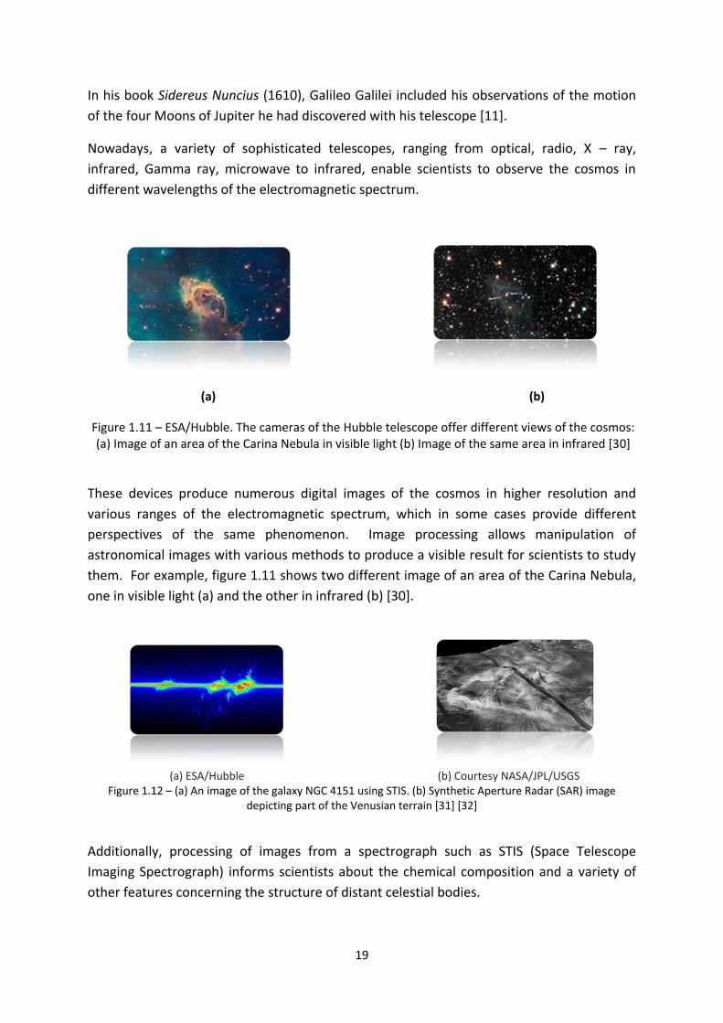
(a) (b)
Figure 1.11 – ESA/Hubble. The cameras of the Hubble telescope offer different views of the cosmos: (a) Image of an area of the Carina Nebula in visible light (b) Image of the same area in infrared [30]
These devices produce numerous digital images of the cosmos in higher resolution and
various ranges of the electromagnetic spectrum, which in some cases provide different
perspectives of the same phenomenon. Image processing allows manipulation of
astronomical images with various methods to produce a visible result for scientists to study
them. For example, figure 1.11 shows two different image of an area of the Carina Nebula,
one in visible light (a) and the other in infrared (b) [30].
(a) ESA/Hubble (b) Courtesy NASA/JPL/USGS
Figure 1.12 – (a) An image of the galaxy NGC 4151 using STIS. (b) Synthetic Aperture Radar (SAR) image depicting part of the Venusian terrain [31] [32]
Additionally, processing of images from a spectrograph such as STIS (Space Telescope
Imaging Spectrograph) informs scientists about the chemical composition and a variety of
other features concerning the structure of distant celestial bodies.

20
One such image is shown in figure 1.12 (a), which informs scientists about the structure of
galaxy NGC 4151 as they can observe the existence of a gas outflow from a black hole
located in it [31].
Another application of image processing is implemented in Synthetic Aperture Radar (SAR),
which is used in remote sensing to provide images of the topography of the Earth as well as
of other planets and satellites in our solar system. Figure 1.12 (b) shows an image of the
surface of Venus as was taken using SAR, a technology which can overcome problems such
as low visibility in the atmosphere [32].
In security applications, CCTV cameras provide images for the surveillance of various private
or public environments. CCTV images provide information which is used for a number of
purposes, as in the case of prevention of crime in private and public environments such as
private houses, schools and military facilities. [33]
This dissertation presents an interactive computer multimedia environment, where the user
uses the web camera to select tracks from a playlist.
21
1.1. Light
1.1.1 The Electromagnetic Spectrum [34]
Light is an electromagnetic wave which consists of small particles (photons) moving at 3x10⁸
m/s. This speed, the speed of light is also defined as the maximum speed in the universe.
The amount of energy a photon carries is defined by E=h v, where h is Planck’s constant.
Every electromagnetic wave is a sinusoidal wave and has a wavelength given by the
expression λ=c/v, where c is the speed of light and v is the frequency.
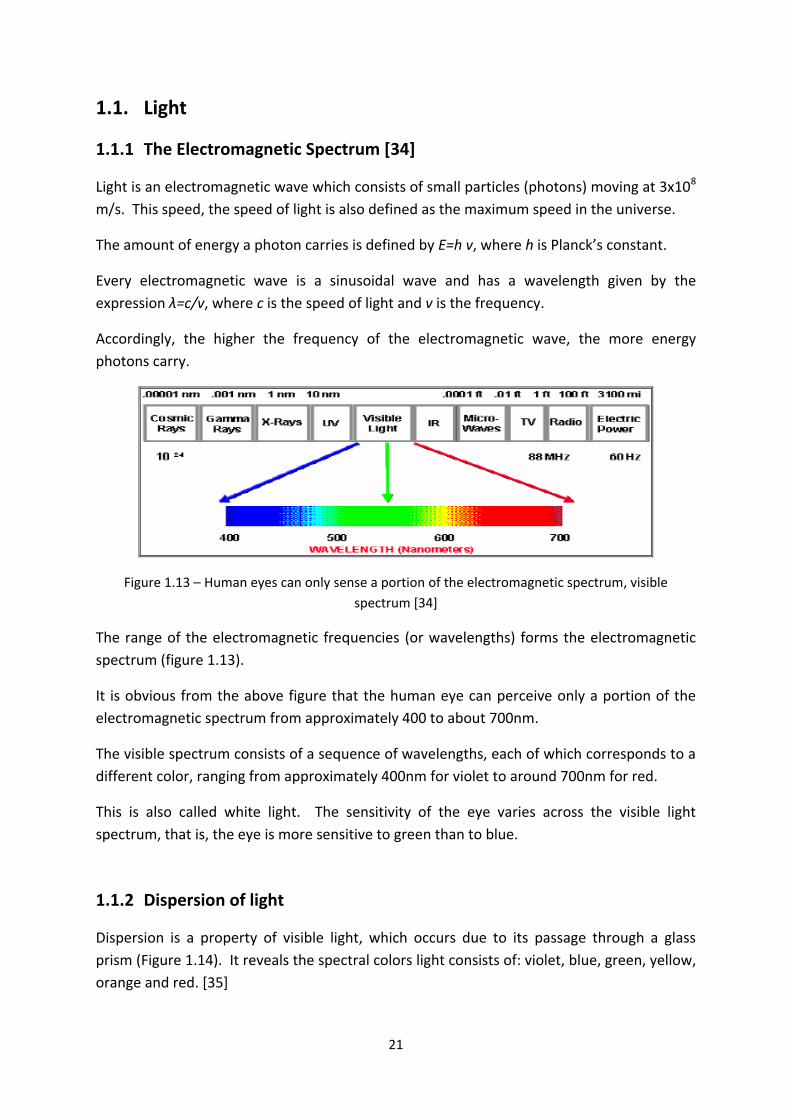
Accordingly, the higher the frequency of the electromagnetic wave, the more energy
photons carry.
Figure 1.13 – Human eyes can only sense a portion of the electromagnetic spectrum, visible
spectrum [34]
The range of the electromagnetic frequencies (or wavelengths) forms the electromagnetic
spectrum (figure 1.13).
It is obvious from the above figure that the human eye can perceive only a portion of the
electromagnetic spectrum from approximately 400 to about 700nm.
The visible spectrum consists of a sequence of wavelengths, each of which corresponds to a
different color, ranging from approximately 400nm for violet to around 700nm for red.
This is also called white light. The sensitivity of the eye varies across the visible light
spectrum, that is, the eye is more sensitive to green than to blue.
1.1.2 Dispersion of light
Dispersion is a property of visible light, which occurs due to its passage through a glass
prism (Figure 1.14). It reveals the spectral colors light consists of: violet, blue, green, yellow,
orange and red. [35]

22
Figure 1.14 – The spectral colors are the result of the refraction of the visible light as it passes
through a glass prism [35]
It is related to the index of refraction of the material through which light is passing. The
speed of light in a non-vacuum material is v = c / n, where n is the index of refraction of the
material through which light is passing. In vacuum, n equals “1” and increases in non-
vacuum, transparent materials. Consequently, as light passes through such materials, its
speed is reduced. [36]
So, based on the index of refraction of a material, light changes speed upon entering
different materials and also changes direction (refraction). [37]
Moreover, since visible light consists of a range of wavelengths, different colors refract at
different angles, with the shorter wavelengths refracting more than the longer one
producing the visible spectrum as shown in figure 1.14. [35]
1.2. Digital Images [27]
A digital image is a 2D array of pixels also expressed as a function f(x, y), where the
dimensions x and y define its size. For example, for x=10 and y=6, then the image would be
an array of 10 x 6 = 60 pixels.
The function f(x, y) defines the intensity at a specific pixel (x, y) in it. In other words, every
pixel in an array contains information of its position and its corresponding intensity.
In the case of a black and white image, the intensity of every pixel on a grayscale is defined
to be equal to 2i shades of gray, where i denotes the bits used to describe that information.
For example, in an 8-bit image, where the intensity information for every pixel uses 8-bits (1
byte), there will be 2i =28 values, that is a range of ‘0 – 255’ levels of grayscale, where ‘0’
(Hex 00) stands for black and ‘255’ (Hex FF) for white.

23
In the case of a color image, every pixel is defined in terms of a combination of a number of
intensity values. For example, for the RGB model, three intensity values are used to define
the levels of blue, green and red.
Figure 1.15 – Every color is encoded as the combination of RGB values
This means that 3 bytes (24-bits) are required to store intensity information for every pixel.
Pure red for example would be [R: 255, G: 0, B: 0], while figure 1.15 shows the encoding for
another shade of red [R: 221, G: 32, B: 36].
Generally, 2D arrays come in the form of 8, 16, 24 and 32-bit formats. Two techniques are
used for storing information regarding color intensities: a) indexed color technique and b)
true color technique.
Figure 1.16 – Image file containing the pixel indices and the palette. The color for every pixel in the image is indexed with a number, so the image processing system can find the corresponding color in
the palette [38]
24
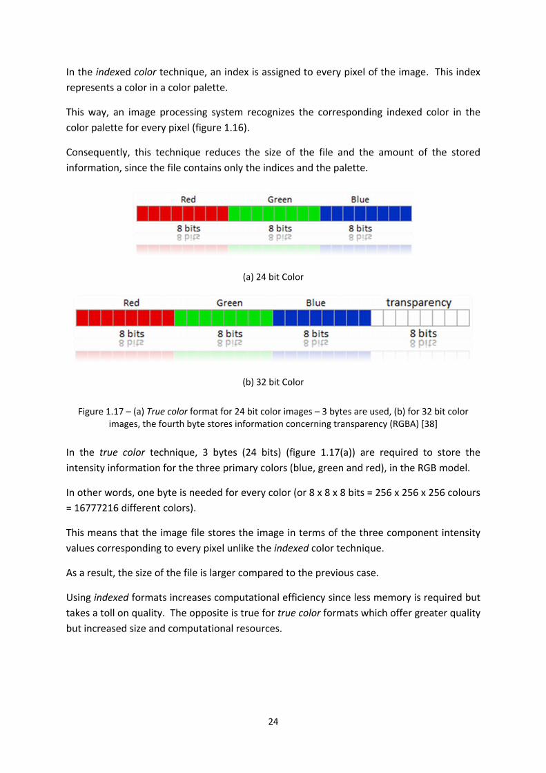
In the indexed color technique, an index is assigned to every pixel of the image. This index
represents a color in a color palette.
This way, an image processing system recognizes the corresponding indexed color in the
color palette for every pixel (figure 1.16).
Consequently, this technique reduces the size of the file and the amount of the stored
information, since the file contains only the indices and the palette.
(a) 24 bit Color
(b) 32 bit Color
Figure 1.17 – (a) True color format for 24 bit color images – 3 bytes are used, (b) for 32 bit color images, the fourth byte stores information concerning transparency (RGBA) [38]
In the true color technique, 3 bytes (24 bits) (figure 1.17(a)) are required to store the
intensity information for the three primary colors (blue, green and red), in the RGB model.
In other words, one byte is needed for every color (or 8 x 8 x 8 bits = 256 x 256 x 256 colours
= 16777216 different colors).
This means that the image file stores the image in terms of the three component intensity
values corresponding to every pixel unlike the indexed color technique.
As a result, the size of the file is larger compared to the previous case.
Using indexed formats increases computational efficiency since less memory is required but
takes a toll on quality. The opposite is true for true color formats which offer greater quality
but increased size and computational resources.

25
1.3. Human Vision
1.3.1 The Human Eye Structure
Figure 1.18 – A simple diagram of the visual processing system
Humans can perceive both stereoscopic and color information [39]. The human visual
system encompasses a variety of structures to convey information about the light, starting
from the eye and moving along the visual nerve and the visual tract to the visual cortical
areas [5]. Human vision is a complex process. A simplified description is described in the
box diagram in figure 1.18.
The eye is a complex organ which acts as the interface between the environment and the
visual processing areas in the brain. It detects light and transforms it into electrochemical
signals, which are transmitted through the optic nerve and the optic tract to visual
information processing areas in the brain. [5]
Figure 1.19 – Representation of a cross-section of the human eye
As was mentioned in section 1.1, human vision is confined within a narrow band of the
electromagnetic spectrum, the visible spectrum. Light travels through the cornea (the
anterior membrane of the eye), the pupil (the opening located at the center of the iris) and
the lens in order to enter the eye (figure 1.19). The pupil is that part of the eye which
Scene
Eye Brain
Processing of
information
Visual
Perception Object
Formation
of image of
object on
retina
Sensory
receptor
26
dilates or constricts depending on the amount of light in the environment, thus controlling
how much light passes. [23]
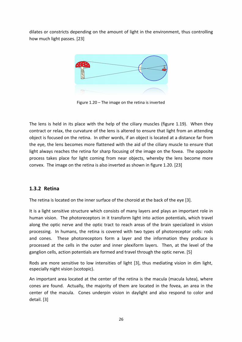
Figure 1.20 – The image on the retina is inverted
The lens is held in its place with the help of the ciliary muscles (figure 1.19). When they
contract or relax, the curvature of the lens is altered to ensure that light from an attending
object is focused on the retina. In other words, if an object is located at a distance far from
the eye, the lens becomes more flattened with the aid of the ciliary muscle to ensure that
light always reaches the retina for sharp focusing of the image on the fovea. The opposite
process takes place for light coming from near objects, whereby the lens become more
convex. The image on the retina is also inverted as shown in figure 1.20. [23]
1.3.2 Retina
The retina is located on the inner surface of the choroid at the back of the eye [3].
It is a light sensitive structure which consists of many layers and plays an important role in
human vision. The photoreceptors in it transform light into action potentials, which travel
along the optic nerve and the optic tract to reach areas of the brain specialized in vision
processing. In humans, the retina is covered with two types of photoreceptor cells: rods
and cones. These photoreceptors form a layer and the information they produce is
processed at the cells in the outer and inner plexiform layers. Then, at the level of the
ganglion cells, action potentials are formed and travel through the optic nerve. [5]
Rods are more sensitive to low intensities of light [3], thus mediating vision in dim light, especially night vision (scotopic).
An important area located at the center of the retina is the macula (macula lutea), where
cones are found. Actually, the majority of them are located in the fovea, an area in the
center of the macula. Cones underpin vision in daylight and also respond to color and
detail. [3]
27
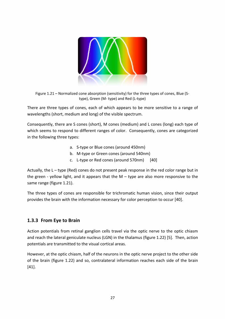
Figure 1.21 – Normalized cone absorption (sensitivity) for the three types of cones, Blue (S-type), Green (M- type) and Red (L-type)
There are three types of cones, each of which appears to be more sensitive to a range of
wavelengths (short, medium and long) of the visible spectrum.
Consequently, there are S cones (short), M cones (medium) and L cones (long) each type of
which seems to respond to different ranges of color. Consequently, cones are categorized
in the following three types:
a. S-type or Blue cones (around 450nm)
b. M-type or Green cones (around 540nm)
c. L-type or Red cones (around 570nm) [40]
Actually, the L – type (Red) cones do not present peak response in the red color range but in
the green - yellow light, and it appears that the M – type are also more responsive to the
same range (figure 1.21).
The three types of cones are responsible for trichromatic human vision, since their output
provides the brain with the information necessary for color perception to occur [40].
1.3.3 From Eye to Brain
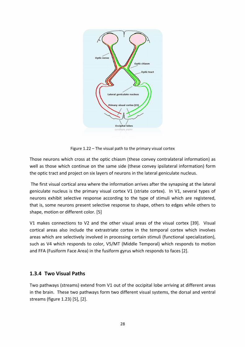
Action potentials from retinal ganglion cells travel via the optic nerve to the optic chiasm
and reach the lateral geniculate nucleus (LGN) in the thalamus (figure 1.22) [5]. Then, action
potentials are transmitted to the visual cortical areas.
However, at the optic chiasm, half of the neurons in the optic nerve project to the other side
of the brain (figure 1.22) and so, contralateral information reaches each side of the brain
[41].
28
Figure 1.22 – The visual path to the primary visual cortex
Those neurons which cross at the optic chiasm (these convey contralateral information) as
well as those which continue on the same side (these convey ipsilateral information) form
the optic tract and project on six layers of neurons in the lateral geniculate nucleus.
The first visual cortical area where the information arrives after the synapsing at the lateral
geniculate nucleus is the primary visual cortex V1 (striate cortex). In V1, several types of
neurons exhibit selective response according to the type of stimuli which are registered,
that is, some neurons present selective response to shape, others to edges while others to
shape, motion or different color. [5]
V1 makes connections to V2 and the other visual areas of the visual cortex [39]. Visual
cortical areas also include the extrastriate cortex in the temporal cortex which involves
areas which are selectively involved in processing certain stimuli (functional specialization),
such as V4 which responds to color, V5/MT (Middle Temporal) which responds to motion
and FFA (Fusiform Face Area) in the fusiform gyrus which responds to faces [2].
1.3.4 Two Visual Paths
Two pathways (streams) extend from V1 out of the occipital lobe arriving at different areas
in the brain. These two pathways form two different visual systems, the dorsal and ventral
streams (figure 1.23) [5], [2].

29
Figure 1.23 – The dorsal stream (red arrow) and the ventral stream (blue arrow). (Arrows were
added to the original image) [7]
The shorter pathway, the dorsal stream, starts from V1 extends to the posterior parietal
cortex. It is the “where” stream as it is responsible for the perception of an object’s size
location and motion. It is also involved in visual guidance of actions. [2]
The ventral stream is a more recent evolutionary visual pathway. It starts from V1 reaches
the inferior temporal lobe. It is responsible for processing fine detail, shape and color. It is
termed the “what” stream and is involved in object recognition. [2]
1.4. Digital Image Algebraic Operation
Algebraic operations fall into two categories: arithmetic and logical as described in the next
two sections.
1.4.1 Arithmetic Operations
Arithmetic operations are performed with images and fall into three categories: a) between
two images (pixel by pixel), b) between an image and a filter and c) between an image and a
coefficient). The resulting image is in any case an image with the same dimensions as the
original one. For example, the result of the operation between two images f(x, y) and g(x,
y), is an image a (x, y), which has the same dimensions x, y (figure 1.24).
f (x, y) g (x, y) a (x, y)
Figure 1.24 – Operation between two images
Operation

30
There are two operations available here: addition and subtraction. Subtraction means that
the resulting image contains only those values which are different between the two initial
images. In the case of a security system, this operation between two scenes will depict only
the intruder.
Figure 1.25 presents an operation between an image f (x, y) and a filter m (x, y) (convolution
process).
f (x, y) m (x, y) a (x, y)
Figure 1.25 – Process to change pixel values in an image
In figure 1.25, the values of the filter m (x, y) (f1 to f9) are applied to the image pixels, a9, a10,
a11, a15, a16, a17, a21, a22, a23. This has an impact on the middle pixel a16 of the image as
described by the following formula:
Finally, an image can be multiplied/divided by a coefficient. In case of dark images,
multiplication by a coefficient value is applied to the image in order to calibrate its
brightness.
Additionally, in the case of very light images, division is applied whereby the pixel values are
divided by a coefficient value.
1.4.2 Logical (Boolean) Operations in Binary Images
Logical operations (Boolean operations) can also be performed between images. They also
take place pixel by pixel and include Boolean operators of AND, OR and NOT whose
combinations can provide other Boolean functions such as NAND, XOR or NOR.
They are based on the fact that in binary images there are two values (either ‘0’ or ‘1’)
which represent black and white, in order to distinguish the important information.
a9 f1+ a10 f2 + a11 f3 + a15 f4 + a16 f5 + a17 f6 + a21 f7 + a22 f8 + a23 f9
Convolution

31
However, in more realistic situations – grayscale images – 256 values are available to
describe various objects contained in the image.
1.4.3 Operations with Matrices
In many cases special filters are required to be applied to part of or the whole of the image.
This process, known as convolution, changes the value of the pixel which is located at the
center of the area where the matrix is applied. As an example, a median filter is needed to
remove the noise which is present in an old image.
1.5. Digital Image Geometric Operations
1.5.1 Image Rotation
In real life situations such as taking photos, sometimes it is necessary to rotate the camera
in order for the desired image to fit.
Image processing enables the rotation of the image. Although images can be rotated at
different angles, the most common rotations involve increments of 900. Performing a 90 -
degree clockwise rotation requires that the row pixel values be copied and then be assigned
to their new location in their corresponding column pixels.
To simplify matters, the example in figure 1.26 shows an array of pixels X with color only in
the top row pixels. The top row pixel values are copied to the right column of image Y
(which also applies to all the rows in the image).
X Y
Figure 1.26 – Rotation. Image X is rotated to the right yielding image Y
900

32
It is important to mention that columns are not copied on the same array of pixels as the
original image, to avoid overwriting the information contained in the pixels of the original
array. The code in ansi – c for rotating an image X by 900 into image Y is shown below:
rotate_90 ( ) {
int i, j, k;
k = Number_of_Columns – 1;
for (i = 0; i < Number_of_Rows; + + i) {
for ( j = 0; j < Number_of_Columns; ++j) {
Y [ j ] [ k ] = X[ i ] [ j ] ;
k = k – 1;
} } }
In the ansi-c code provided above, variables i and j represent the horizontal and vertical
dimensions of array X respectively. Variable k stands for the number of columns of the
array which are copied from array X (original mage) to array Y (destination image). Starting
from “0”, rotation by 900 to the right stops when the value of k reaches ‘number of columns
– 1’.
1.5.2 Image Flip (Horizontal and Vertical)
As in the previous case, flipping an image relies on the same concept. However, in the case
of a vertical flip, the bottom row pixels of the image X (figure 1.27) are the start point and
are copied to the top row of pixels in image Y.
X Y
Figure 1.27 – Image X is vertically flipped by 1800 yielding image Y

33
In the case of a horizontal flip, all columns in the original image are copied to the destination
array of pixels. More specifically, the first column in image X (original) is copied to the last
column in image Y. Figure 1.28 below shows an example of an image flipped horizontally.
a b
Figure 1.28 – Housekeeper Robot image ‘a’ is flipped horizontally producing image ‘b’
The code in ansi-c for flipping an image X vertically (into image Y) is shown below:
flip ( ) {
int i, j, k;
k = Number_of_Rows – 1;
for (i = 0; i < Number_of_Columns; + + i) {
for (j = 0; j < Number_of_Rows; ++j) {
Y [ k ] [ j ] = X[ i ] [ j ] ;
k = k – 1;
}
}
}
In the ansi-c code provided above, variables i and j represent the horizontal and vertical
dimensions of array X respectively. Variable k stands for the number of columns of the
array which are copied from array X (original mage) to array Y (destination image).
Variables i and j define the position of a pixel in image X, starting from the bottom row.
Flipping the image vertically stops when the value of k reaches ‘number of rows – 1’.

34
1.6. Digital Image Formats and Storage [42]
An image is a representation of an object or a scene in an electronic form. There are
basically two types of images: raster (or bit-mapped) images and vector images.
A raster image (figure 1.29) is a representation of an image in the form of a rectangular grid
of pixels. Each pixel in the grid is assigned a specific value of bits which map their intensity
and color values. The number of pixel elements employed for encoding pixel information
can be used to distinguish between different types of raster images.
(a) (b)
Figure 1.29 – A raster image: Zooming in on image (a) reveals the raster grid of pixels (b) [43]
For example, in black and white images, a pixel can be represented in the form of one (1)
byte (8 bits) for 256 gray levels. In color images, every pixel is mapped by three numbers
which define the levels of blue, green and red (primary colors). So, in the case of 256 levels
for every primary color, three (3) bytes (24 bits or 24 bit color) are used to define the levels
of the primary colors in a pixel. One problem with raster images is that the pixels become
visible when they are resized, so in order to increase the quality of the image, higher
resolution is needed. This however, can take a toll on the size of the storage file. Sources of
raster images include digital cameras and scanners.
Vector images consist of lines and curves. The information about the image is contained in
mathematical expressions (vectors), contrary to raster images, which make use of pixel
information. Vectors hold a range of information which includes direction, start and end
points, color or grade of the vector. One advantage of using vector images is that they
maintain their clarity when they are resized contrary to raster images which tend to lose
their clarity as pixel elements become more discernible. Vector images are produced and
35
handled with drawing programs and they are stored in various file forms, some of which
include: .ai, .cdr, .svg and .dfx.
Raster images are stored in a file format which defines the name of the file and the type, for
example, battery.png. The most commonly used formats of raster images are discussed
below in section 1.6.1.
1.6.1 Formats of Digital Images [42]
In the following lines, the most commonly used digital still image formats are described.
GIF
This is an old indexed format supporting 256 colors (8-bit quality). This means that, every
color encoded in a GIF file does not contain the information about the color but rather is
assigned a number (index), which represent that color in a palette of 256 colors. It is
suitable for storing images with few colors such as web images, logos and diagrams.
BMP (Bit-mapped)
BMP images are uncompressed images used in Microsoft windows. As a result, their large
size renders them difficult to handle large images.
JPEG or JPG (Joint Photographic Experts Group)
This format is extensively used on the Internet (web pages) as well as by digital cameras due
to their compression efficiency which stores data in very small files. The method also
provides the option to save images in JPEG files of various size and quality by selecting
compression level. They support 24-bit truecolor images and 8-bit grayscale images.
PNG (Portable Network Graphics)
This format was originally the successor to the GIF format. The PNG format supports 24 or
32-bit truecolor images, grayscale images and indexed (8-bit) images. They are suitable for
the Internet which was their original purpose and also for animation.
TIFF (Tagged Image File Format)
Originally, it was developed to handle grayscale images. It is a flexible form of storing
images as it handles grayscale, indexed images, RGB images, CMYK images and also 8, 16 ,
24, or 48-bits per color (red, green, blue). Extension of the file where data is stored can be
either TIFF or TIF.
36
1.7. Color models – Fundamentals [23]
As was mentioned in section 1.1, the visible spectrum consists of a sequence of wavelengths
that span from approximately 400nm to approximately 700nm (Figure 1.13). Passing
through a prism, the visible light spectrum (or the wavelengths that make it up) is separated
into the colors of the rainbow (spectral colors) each of which consists of numerous shades.
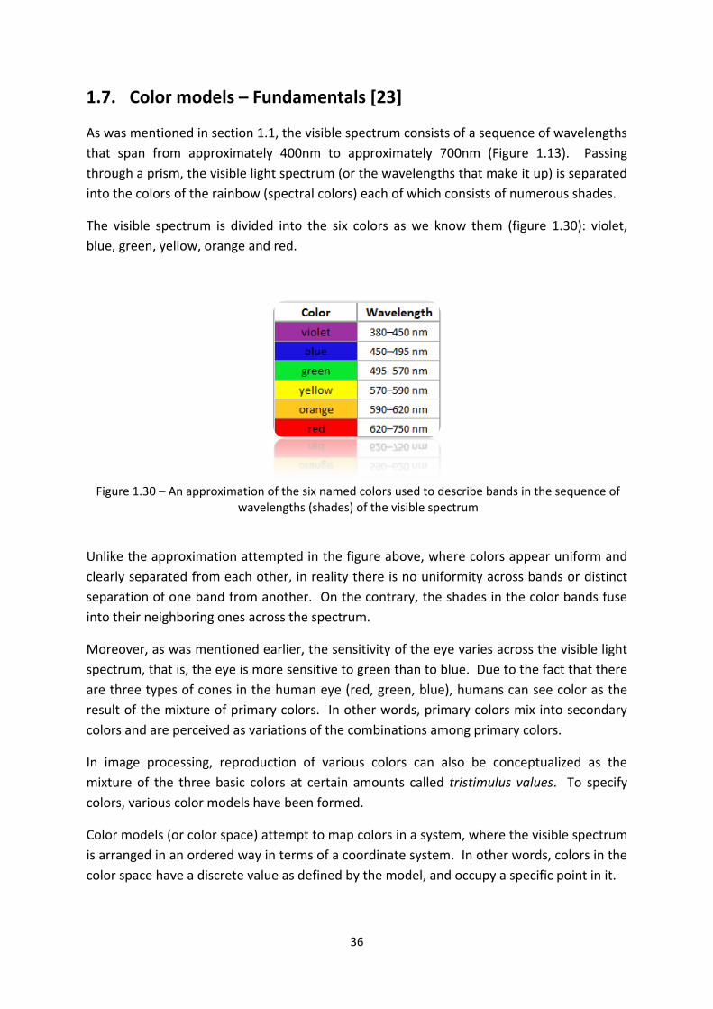
The visible spectrum is divided into the six colors as we know them (figure 1.30): violet,
blue, green, yellow, orange and red.
Figure 1.30 – An approximation of the six named colors used to describe bands in the sequence of
wavelengths (shades) of the visible spectrum
Unlike the approximation attempted in the figure above, where colors appear uniform and
clearly separated from each other, in reality there is no uniformity across bands or distinct
separation of one band from another. On the contrary, the shades in the color bands fuse
into their neighboring ones across the spectrum.
Moreover, as was mentioned earlier, the sensitivity of the eye varies across the visible light
spectrum, that is, the eye is more sensitive to green than to blue. Due to the fact that there
are three types of cones in the human eye (red, green, blue), humans can see color as the
result of the mixture of primary colors. In other words, primary colors mix into secondary
colors and are perceived as variations of the combinations among primary colors.
In image processing, reproduction of various colors can also be conceptualized as the
mixture of the three basic colors at certain amounts called tristimulus values. To specify
colors, various color models have been formed.
Color models (or color space) attempt to map colors in a system, where the visible spectrum
is arranged in an ordered way in terms of a coordinate system. In other words, colors in the
color space have a discrete value as defined by the model, and occupy a specific point in it.

37
Three of the most common color models used in digital image processing are: the RGB (red,
green, blue) model, the CMYK (cyan, magenta, yellow and black) and the HSB (HSV) model.
1.7.1 RGB [44]
In this model, the principal idea is that reproduction of colors occurs by mixing (adding) the
three primary colors as shown in figure 1.31. White is the result of mixing the three primary
colors (blue, green and red) while black is the result of the absence of color.
It is also obvious from image 1.28 that when two primary colors mix, the secondary colors
yellow, cyan and magenta are produced. In other words
Figure 1.31 – The RGB additive mixing model.
Another way of conceptualizing this model is in terms of the RGB color space (figure 1.32),
where every color is the combination of the three primary colors expressed as a point in a
3D cube.
Figure 1.32 – RGB space color

38
In other words, different values of red, green and blue will define a different color as a point
in the 3D cube space. For example, (0, 0, 0) represents black and (1, 1, 1) represents white,
both located in the diagonally opposite corners of the 3D cube in figure 1.32.
The RGB model is used for the reproduction of colors in computer graphics and displays,
such as television, computer and video game displays.
1.7.2. CMYK [23]
The idea in this model is the reverse to the RGB model. In the CMYK model, the primary
colors are considered to be cyan, magenta and yellow.
More precisely, contrary to the RGB model, CMYK considers white to represent the absence
of color. Black is the result of the combination of equal quantities of cyan, magenta and
yellow (figure 1.33).
Figure 1.33 – The CMYK subtractive model
A color in this model is produced because another color subtracts all the other wavelengths
except the one that defines that color. For example, in the case of blue, it is the result of
the absorption of cyan by magenta.
It is worth mentioning that the CMYK model is derived from the CMY model, where black
was not used. However, the use of black (thus the addition of the K symbol) improves the
quality of the colors produced with this model.
The fact that the CMYK model considers that white stands for the absence of color renders
it ideal for printing. Since the color of the page is white, this means that if a color would be
placed on it, it would be perceived as such because all the other wavelengths would be
absorbed (subtracted) by the white of the page.

39
1.7.3. HSB/HSV
In HSB (Hue, Saturation and Brightness) or HSV (Hue, Saturation and Value) color model (or
otherwise called HSI – Hue, Saturation and Intensity), colors are placed in a 3D space which
is enclosed by two cones. This model resembles the way humans perceive color. The
longitudinal axis represents the grayscale (neutral or achromatic colors) with black at its
bottom end and white at the top.
In this model, colors are located on a disk moving along the longitudinal axis towards either
end. The three components, Hue, Saturation, and Brightness, combine to form every color
in the visible spectrum – B is replaced with Intensity – I).
Brightness (0 – 1)
(Value along the longitudinal axis 0 -1)
Saturation (0 – 1)
Hue (00 - 3600) Color
Black
(radius = 1 or saturation = 1)
White
(Value along the radius of disk 0 – 1)
1 00 Red
0 0.5 1
1 600 Yellow 0 0.5 1 1 1200 Green 0 0.5 1
1 1800 Cyan 0 0.5 1
1 2400 Blue 0 0.5 1
1 3000 Magenta 0 0.5 1
Figure 1.34 – Hue component in the HSB model: Specific angular positions on the disk
correspond to the colors as we know them
Brightness (Value or Intensity) varies along the longitudinal axis ranging between 0 (for
black) and 1 (for white). Different angles around the central longitudinal axis (00 – 3600)
yield different values of hue while variation along the radius of the disk (ranging between 0
– 1) yields different values of saturation (the degree to which a color is mixed with white).
In other words, hue defines the position of the area of the colors at specific angles on the
disk for any given brightness.
This is elaborated more explicitly in figure 1.34, which shows the position of the six colors on
the disk as the angle varies from 00 to 3600 (the step is 600) for Saturation = 1 and Brightness
= 0.5.
40
Chapter 2: Segmentation
2.1. The Basic Concept
A challenging and complex process in image processing is segmentation of real-world
images, whereby discreet regions must be defined in an intelligent and correct way. At a
later stage, well-identified segmented areas can lead to an effective object recognition
process.
There are various segmentation methods some of which are: Thresholding, edge detection,
region detection, clustering, deformable models such as snakes, as well as split – merge and
group algorithms using tree structure.
2.2. Segmentation Methods and Techniques
2.2.1. Thresholding [45]
Thresholding is a very well-known and widely used technique for the segmentation of
simple images. It is an intensity-based technique whereby segmentation of areas is
achieved by selecting pixels with similar intensities.
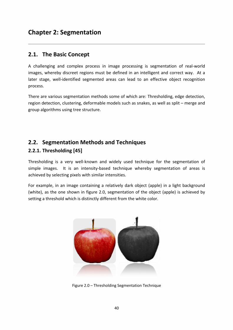
For example, in an image containing a relatively dark object (apple) in a light background
(white), as the one shown in figure 2.0, segmentation of the object (apple) is achieved by
setting a threshold which is distinctly different from the white color.
Figure 2.0 – Thresholding Segmentation Technique

41
It is common knowledge that in grayscale images the range of intensities of gray color varies
from 0 (black) to 255 (white) (Figure 2.1). So, an important step in this direction is the
analysis of the image into a histogram which provides a distribution of pixel intensities of
the image in gray scale.
Figure 2.1 – Histogram of the image in figure 2.1
In the histogram above, the threshold value is set to 250, lower than 255 which is the upper
limit of the range of colors, in order to segment the apple from the background. This value
has been selected, due to some light areas on the surface of the apple albeit not as white as
the background.
Therefore, there is a distinct threshold that allows separation of the two classes (apple and
background).
If the image above is represented by f(x, y), where white is the background and darker areas
are the object (apple; both lobes are part of the apple image), given that the threshold level
is set at T, the following rule applies for every point (x, y) in the image:
In other words, every point (x, y) in the image f(x, y) is part of the object (apple), if their
intensities are below the threshold level. In the opposite case, their intensities are equal to
or below the threshold level and consequently they are part of the white background.
Another real case segmentation example is a ship floating in the sea. Ideally, the gray scale
representation of the ship would correspond to a single line in histogram, which would
represent the intensity of all the pixels located on the ship and a second line would
correspond to the intensity of the pixels belonging to the sea. That would happen in case
the gray scale intensities along both areas (the ship and the sea) do not vary.

42
However, there is no such ideal situation in reality due to a number of factors such as
discontinuities in color, lack of uniformity of texture, shadowing and reflections of light due
to differences in surface orientation.
As a result, the ensuing histogram will be the one shown in figure 2.2, where the first group
of lobes (left) correspond to a range of pixel intensities belonging in the ship and the second
group of lobes to another range of pixel intensities which belong in the sea.
Figure 2.2 – Histogram representation of the image [46]
Factors like the aforementioned can introduce overlapping between the lobes in the
histogram, which in more complex images would render the segmentation task ineffective.
In other words, to achieve successful thresholding, overlapping between the lobes that
represent the objects in the histogram must not occur.
However, in complex images such as the brain scans medical images, thresholding alone is
not sufficient, and requires additional more sophisticated segmentation techniques for
accurate delineation of important areas.
The simplicity of the technique, makes thresholding extremely applicable in cases where
lighting is smooth and controlled and the color of the objects and the background on the
histogram differ (e.g. industrial environments), providing ideal conditions for an
unsupervised automatic system.
2.2.2 Sobel Masks [23]
More complex images would require the implementation of different techniques. One such
technique is Sobel Masks which are used to detect edges in images.
43
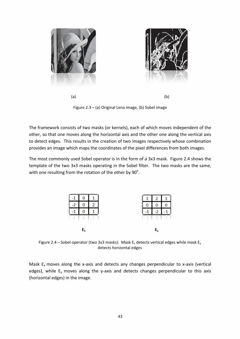
(a) (b)
Figure 2.3 – (a) Original Lena image, (b) Sobel image
The framework consists of two masks (or kernels), each of which moves independent of the
other, so that one moves along the horizontal axis and the other one along the vertical axis
to detect edges. This results in the creation of two images respectively whose combination
provides an image which maps the coordinates of the pixel differences from both images.
The most commonly used Sobel operator is in the form of a 3x3 mask. Figure 2.4 shows the
template of the two 3x3 masks operating in the Sobel filter. The two masks are the same,
with one resulting from the rotation of the other by 90o.
Ex Ey
Figure 2.4 – Sobel operator (two 3x3 masks): Mask Ex detects vertical edges while mask Ey
detects horizontal edges
Mask Ex moves along the x-axis and detects any changes perpendicular to x-axis (vertical
edges), while Ey moves along the y-axis and detects changes perpendicular to this axis
(horizontal edges) in the image.
44
The basic principle is that the center column of mask Ex and the center row of mask Ey are
zero. This means that when the masks are applied to the image, only the weights of the
masks contribute to the calculation of the difference of the pixel values in the image.
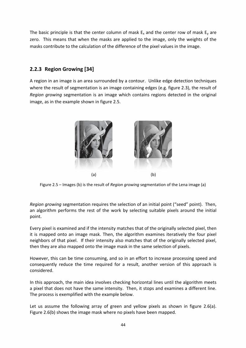
2.2.3 Region Growing [34]
A region in an image is an area surrounded by a contour. Unlike edge detection techniques
where the result of segmentation is an image containing edges (e.g. figure 2.3), the result of
Region growing segmentation is an image which contains regions detected in the original
image, as in the example shown in figure 2.5.
(a) (b)
Figure 2.5 – Images (b) is the result of Region growing segmentation of the Lena image (a)
Region growing segmentation requires the selection of an initial point (“seed” point). Then, an algorithm performs the rest of the work by selecting suitable pixels around the initial point.
Every pixel is examined and if the intensity matches that of the originally selected pixel, then it is mapped onto an image mask. Then, the algorithm examines iteratively the four pixel neighbors of that pixel. If their intensity also matches that of the originally selected pixel, then they are also mapped onto the image mask in the same selection of pixels.
However, this can be time consuming, and so in an effort to increase processing speed and consequently reduce the time required for a result, another version of this approach is considered.
In this approach, the main idea involves checking horizontal lines until the algorithm meets a pixel that does not have the same intensity. Then, it stops and examines a different line. The process is exemplified with the example below.
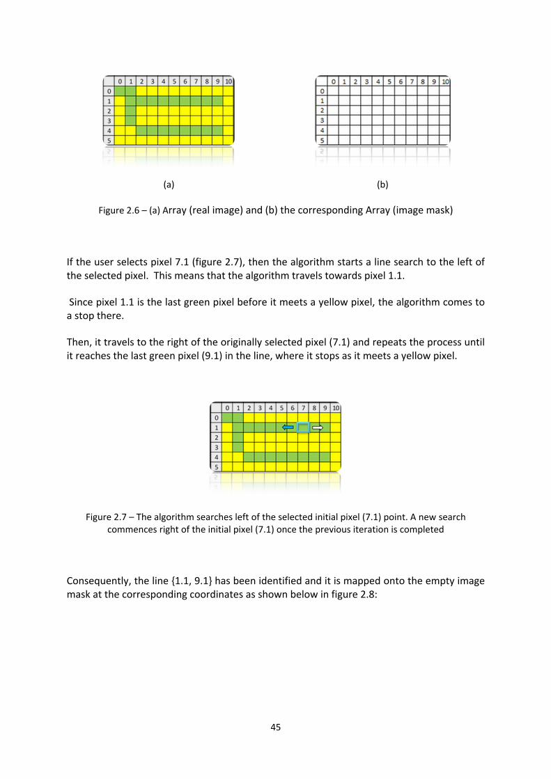
Let us assume the following array of green and yellow pixels as shown in figure 2.6(a). Figure 2.6(b) shows the image mask where no pixels have been mapped.
45
(a) (b)
Figure 2.6 – (a) Array (real image) and (b) the corresponding Array (image mask)
If the user selects pixel 7.1 (figure 2.7), then the algorithm starts a line search to the left of the selected pixel. This means that the algorithm travels towards pixel 1.1.
Since pixel 1.1 is the last green pixel before it meets a yellow pixel, the algorithm comes to a stop there.
Then, it travels to the right of the originally selected pixel (7.1) and repeats the process until it reaches the last green pixel (9.1) in the line, where it stops as it meets a yellow pixel.
Figure 2.7 – The algorithm searches left of the selected initial pixel (7.1) point. A new search commences right of the initial pixel (7.1) once the previous iteration is completed
Consequently, the line {1.1, 9.1} has been identified and it is mapped onto the empty image mask at the corresponding coordinates as shown below in figure 2.8:

46
(a) (b)
Figure 2.8
The next step for the algorithm is to check each pixel directly above those pixels already detected in line {1.1 - 9.1}. So, the algorithm starts with pixel 1.0, which is directly above pixel 1.1 (the left end of the previously detected line), moving to 2.0, 3.0 all the way to 9.0.
(a) (b)
Figure 2.9
When the search is completed, the algorithm finds that only pixel 1.0 is green, so the algorithm repeats the search process to the left of that pixel to find green pixels (figure 2.9(a)). It completes the search at pixel (0.0) in that line. Then, the algorithm searches to the right of pixel 1.1 and since there are no green pixels, the newly detected line {0.0 - 1.0} is mapped onto the image mask at the corresponding coordinates (figure 2.10), as previously.
Figure 2.10

47
Then, the algorithm searches directly below the originally selected line (pixels 1.1, 1.2, 1.3, 1.4, 1.5, 1.6, 1.7, 1.8, 1.9). There is only one green pixel below that line, pixel 1.2. The algorithm searches to the left and then to the right of pixel 1.2 (figure 2.11) and the search finishes as there are no other green pixels in that line. Pixel 1.2 is mapped onto the image mask, as in the previous cases (figure 2.12).
Figure 2.11
Figure 2.12
Next, the algorithm returns to line {0.0 - 1.0} to check above it for green pixels. There are no green pixels above that line. So, the algorithm searches below the same line for green pixels but there are no green pixels to be mapped either.
Then, the algorithm returns to line {1.2}, where there is only one green pixel and searches above it in line 1 but there are no green pixels to be mapped either. Next, it searches below (in line 3) and finds only one green pixel in that line, that is, pixel 3.1.
The algorithm repeats the process by searching to the left of that pixel and then to the right, but there are no green pixels in either direction. So, it maps pixel {3.2}. Then, the algorithm searches above pixel {3.2} as it forms a line, but no green pixels can be mapped.
Next, the algorithm searches below that line and the process continues with iterations until all green pixels have been examined and are finally mapped onto the image mask.
One point that needs to be mentioned here is that all green pixels detected by the algorithm are assigned value ‘1’ while pixels not detected as green are assigned the value ‘0’. Generally, the process involves the following steps:
0 1 2 3 4 5 6 7 8 9 10
0
1
2
3
4
5
0 1 2 3 4 5 6 7 8 9 10
0
1
2
3
4
5
0 1 2 3 4 5 6 7 8 9 10
0
1
2
3
4
5
48
An initial point is selected to provide the pixels that will determine the predefined properties
The pixel is assigned value ‘1’
Iterations compare neighbouring pixels with those at the initial selection point by checking pixels in lines, until no more pixels of the same value are found in the same line
Lines detected are mapped onto an image mask as segments, where pixels are assigned values ‘1’. All other pixels are assigned value ‘ 0’
The process is terminated when no more pixels can be examined
A new seeding point is selected for a new search to start
2.2.4 Active Contours [28]
Another method to delineate objects in 2D images is active contours which are also known
as snakes.
An important step to initiate snakes is a starting point whereby an initiating contour (ex. an
ellipse) is placed inside or outside the object required to be segmented. The contour
expands like a balloon or shrinks respectively, so as to delineate the boundaries of the
object.
One widely used active contours method is the Greedy algorithm. The idea underlying the
Greedy algorithm is that the external energy at the initializing point has a maximum value
while at the contour of the target object it has a minimal value.
More specifically, if the starting point near a target object is , the Greedy active
algorithm reaches a point , which is part of the contour of the target object, by means of
minimizing the energy in the function below:
To ensure effective segmentation of the target object, it is necessary to define the
parameters involved in the minimization of the energy of the aforementioned function.
Depending on the snake, there are several possible factors that could be introduced but
some of the most important ones are:
Continuity
It is an internal parameter, which allows the snake pixels to define their positioning towards
neighbor pixels. This ensures that the distance between them is approximately the average
distance between the pixels belonging to the snake. Thus, the snake can expand and
maintain the distance between snake pixels equal.

49
Curvature
As an internal parameter, it controls the position of the snake and ensures its smoothness in
terms of maintaining the minimal amount of the curvature. It achieves this by maintaining
the angle between snake neighbors at maximum value.
Gradient
As an external parameter, it enables the snake to guide itself towards areas characterized
by large gradient.
Balloon (pressure)
This parameter gives the snake ellipse balloon-like properties. That is, it allows it to expand
or shrink like a balloon and proceed over edges which are weak or stop at weaker.
2.2.5 K-means Clustering [47], [48]
K-means is an iterative semi-supervised clustering algorithm. The algorithm assigns the data
belonging in an object to a cluster, based on the Euclidian distance. Depending on the
number of objects existing in an image, the user may select K clusters.
The method is implemented in two stages. First, there is selection of initial points belonging
in objects contained in an image. Start points are used to define the objects.
Then, the algorithm selects randomly a point in the image, calculates the Euclidean distance
to the start points and assigns it to the nearest start point to form a cluster. The centroid of
the cluster is calculated and every time a new point is added to the cluster the centroid is
reassigned. The process is completed when there are no more points left to cluster.
Generally, one of the advantages of K-means algorithm is the ease of implementation.
However, careful selection of the value of k (manual selection of initial points) prior to the
application of the algorithm is needed as it is associated with the quality of the output
images.
2.2.6 Hough Forests for Object Detection
Originally, Hough transform was developed to detect lines, circles or eclipses [49]. Later on
Generalized Hough transform was introduced to deal with more complex shapes.
Generalized Hough transform is used in Hough forests to locate an object in real-world
images [50].

50
More specifically, the main idea underpinning Hough forests is that a number of parts which
belong to objects of the same category (e.g. bicycle) can help pinpoint the location of an
object of the same class in real-world images. Hough forests consist of a number of Hough
trees and the way they are grown is similar to the way Random forests are grown [48].
Random forests are the result of grouping together a number of Random trees, each of
which actually consists of nodes, branches and leaves, which grow from a root node. Each
of the nodes contains a binary function.
As mentioned earlier, objects in real-world images are located using class-specific parts of a
number of objects of the same category which function as representative parts of that class.
Consequently, when one such representative part image is fed to the root node of a tree, it
ends up in a leaf following the path indicated by the outcome of the binary functions in the
nodes it goes through.
It is important to note that a Random forest is associated with one category of images as in
the case of Hough forests, for example vehicles or people in the streets. [50]
To exemplify the way binary functions work, figure 2.13(b) shows a simplified example of a
decision (binary) tree for the classification of the input (c) based on their color (red, green,
yellow).
(a)
(b) (c)
Figure 2.13 – (a) The structure of a tree in general, (b) A decision (binary) tree which classifies the
input (c) (here red, green and yellow stars are assumed to be the same size and shape)

51
As shown in the example, the data i in 2.13(c) is fed to the root node and a binary function is
applied. The data is sent down the branches and follows a route based on the decisions
(true or false) at the nodes, until they reach a leaf.
These functions stored at the nodes need to undergo training. Prior to training, a number of
objects of interest from the same category are delineated in the training images by means
of bounding areas. This allows small areas from within and outside the bounding area to be
selected – image patches.
Image patches are of equal size and are distinguished in two types:
Object patches
Background patches [50]
Object patches come from within the bounding area of the class of objects that is defined,
such as car, whereas background patches originate from outside bounding areas.
Each tree is grown using a number of object and background patches at the root node.
During the supervised training of the trees, the root node in each tree is split into two other
nodes based on a binary function.
As the procedure continues and the ensuing nodes split, branches are formed with a leaf at
their end. Through this process, the nodes of a tree learn the parameters of the algorithm
stored in them and which split the data in the most efficient way.
At the end of the training process, each leaf node on a tree stores the result of the training
in the form of a distribution, for example (i, L), where L stands for the label and i for a
feature vector representing the input data. L takes either 1 for class representative patches
or 0 for non-class representative patches.
In line with the random forest framework, Hough forests are a framework for object
recognition. As in the case of Random forests, first numerous random trees are created in a
supervised manner to train the model. Then, the system searches for the object of interest
in each of the trees to locate the possible area that includes this object in the image. [50]
The difference from Random forests is that Hough forests store three parameters instead of
two in the leaf nodes, that is, (in, Ln, vn) where in stands for a feature vector corresponding to
a set of features extracted from the input data, Ln stands for the class label, and the
additional vn represents a 2D distance vector indicating the distance between the center of
an object patch and the centroid of the image object.
It is important at this point to clarify that, during supervised training, the class information
stored in the tree leaves also stores the corresponding data concerning the distance vector.
More specifically, if class is Ln=1 (for patches belonging in an object), this means that this
information is stored in the tree leaves along with the distance vector.
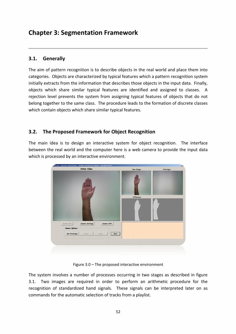
52
Chapter 3: Segmentation Framework
3.1. Generally
The aim of pattern recognition is to describe objects in the real world and place them into
categories. Objects are characterized by typical features which a pattern recognition system
initially extracts from the information that describes those objects in the input data. Finally,
objects which share similar typical features are identified and assigned to classes. A
rejection level prevents the system from assigning typical features of objects that do not
belong together to the same class. The procedure leads to the formation of discrete classes
which contain objects which share similar typical features.
3.2. The Proposed Framework for Object Recognition
The main idea is to design an interactive system for object recognition. The interface
between the real world and the computer here is a web camera to provide the input data
which is processed by an interactive environment.
Figure 3.0 – The proposed interactive environment
The system involves a number of processes occurring in two stages as described in figure
3.1. Two images are required in order to perform an arithmetic procedure for the
recognition of standardized hand signals. These signals can be interpreted later on as
commands for the automatic selection of tracks from a playlist.
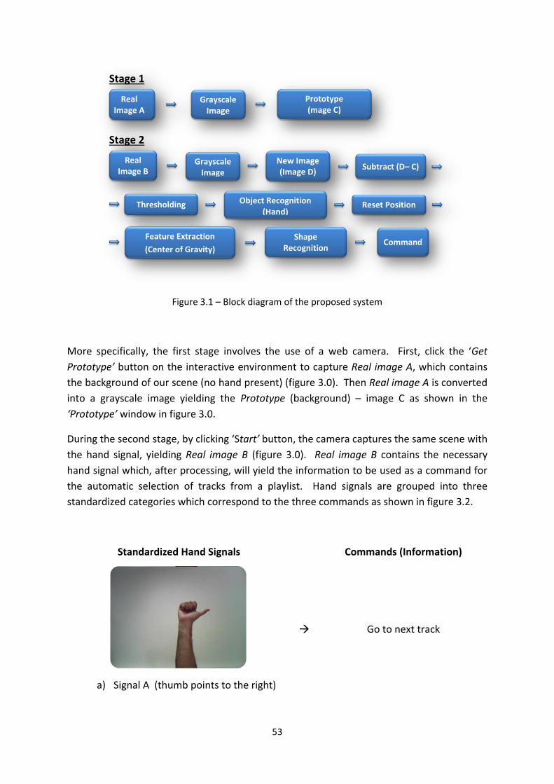
53
Figure 3.1 – Block diagram of the proposed system
More specifically, the first stage involves the use of a web camera. First, click the ‘Get
Prototype’ button on the interactive environment to capture Real image A, which contains
the background of our scene (no hand present) (figure 3.0). Then Real image A is converted
into a grayscale image yielding the Prototype (background) – image C as shown in the
‘Prototype’ window in figure 3.0.
During the second stage, by clicking ‘Start’ button, the camera captures the same scene with
the hand signal, yielding Real image B (figure 3.0). Real image B contains the necessary
hand signal which, after processing, will yield the information to be used as a command for
the automatic selection of tracks from a playlist. Hand signals are grouped into three
standardized categories which correspond to the three commands as shown in figure 3.2.
Standardized Hand Signals Commands (Information)
a) Signal A (thumb points to the right)
Go to next track
Stage 1
Stage 2
Real Image B
Grayscale Image
New Image (Image D)
Subtract (D– C)
Thresholding Object Recognition (Hand)
Reset Position
Feature Extraction
(Center of Gravity)
Shape Recognition
Command
Real Image A
Grayscale Image
Prototype (mage C)
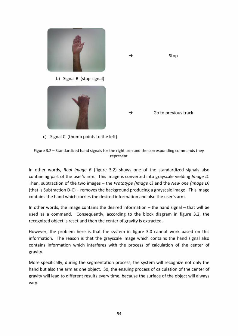
54
b) Signal B (stop signal)
Stop
c) Signal C (thumb points to the left)
Go to previous track
Figure 3.2 – Standardized hand signals for the right arm and the corresponding commands they
represent
In other words, Real image B (figure 3.2) shows one of the standardized signals also
containing part of the user’s arm. This image is converted into grayscale yielding Image D.
Then, subtraction of the two images – the Prototype (Image C) and the New one (Image D)
(that is Subtraction D-C) – removes the background producing a grayscale image. This image
contains the hand which carries the desired information and also the user’s arm.
In other words, the image contains the desired information – the hand signal – that will be
used as a command. Consequently, according to the block diagram in figure 3.2, the
recognized object is reset and then the center of gravity is extracted.
However, the problem here is that the system in figure 3.0 cannot work based on this
information. The reason is that the grayscale image which contains the hand signal also
contains information which interferes with the process of calculation of the center of
gravity.
More specifically, during the segmentation process, the system will recognize not only the
hand but also the arm as one object. So, the ensuing process of calculation of the center of
gravity will lead to different results every time, because the surface of the object will always
vary.

55
Consequently, there will be errors in the interpretation of the extracted information as the
center of gravity will always shift towards the areas of greater gravity depending on the
varying surface of the arm.
A solution must be found in order to take into account only the hand in the process of
calculation of the center of gravity. This can be achieved if the user wears a long sleeved
dark color jacket as shown in figure 3.3 below.
Figure 3.3 – By wearing a long sleeved dark color jacket, the arm is covered. Thresholding will yield only the hand to be used in the process of calculation of center of gravity, excluding any
interference from the arm surface.
Now, the unnecessary information – the part of the arm below the wrist – is covered with
the sleeve. Since the color of the sleeve is not the same as the color of the hand, a simple
segmentation technique, namely thresholding, removes that unnecessary information from
the image.
By setting appropriate threshold levels, the useless information is segmented and removed,
leaving an image which contains only the hand and consequently the desired information it
conveys (the signal).
At this step, it is important for the process of recognition to reset the position of the object
contained in the image (top left corner). In this way, the center of gravity of the object is
extracted. The shape of the hand is recognized as one of the three categories of hand
signals associated with the corresponding command (figure 3.2) to be used for appropriate
selection of tracks from a playlist.
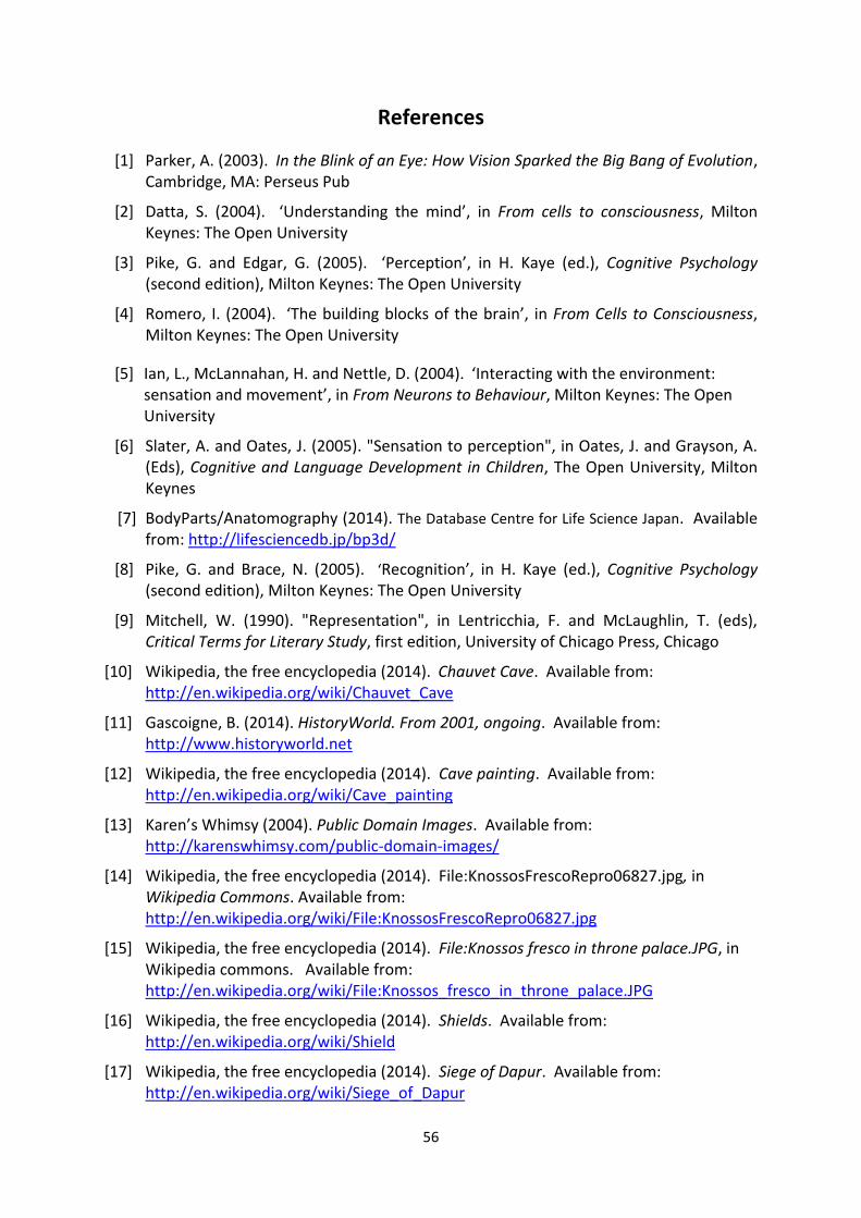
56
References
[1] Parker, A. (2003). In the Blink of an Eye: How Vision Sparked the Big Bang of Evolution, Cambridge, MA: Perseus Pub
[2] Datta, S. (2004). ‘Understanding the mind’, in From cells to consciousness, Milton Keynes: The Open University
[3] Pike, G. and Edgar, G. (2005). ‘Perception’, in H. Kaye (ed.), Cognitive Psychology (second edition), Milton Keynes: The Open University
[4] Romero, I. (2004). ‘The building blocks of the brain’, in From Cells to Consciousness, Milton Keynes: The Open University
[5] Ian, L., McLannahan, H. and Nettle, D. (2004). ‘Interacting with the environment: sensation and movement’, in From Neurons to Behaviour, Milton Keynes: The Open University
[6] Slater, A. and Oates, J. (2005). "Sensation to perception", in Oates, J. and Grayson, A. (Eds), Cognitive and Language Development in Children, The Open University, Milton Keynes
[7] BodyParts/Anatomography (2014). The Database Centre for Life Science Japan. Available from: http://lifesciencedb.jp/bp3d/
[8] Pike, G. and Brace, N. (2005). ‘Recognition’, in H. Kaye (ed.), Cognitive Psychology (second edition), Milton Keynes: The Open University
[9] Mitchell, W. (1990). "Representation", in Lentricchia, F. and McLaughlin, T. (eds), Critical Terms for Literary Study, first edition, University of Chicago Press, Chicago
[10] Wikipedia, the free encyclopedia (2014). Chauvet Cave. Available from: http://en.wikipedia.org/wiki/Chauvet_Cave
[11] Gascoigne, B. (2014). HistoryWorld. From 2001, ongoing. Available from: http://www.historyworld.net
[12] Wikipedia, the free encyclopedia (2014). Cave painting. Available from: http://en.wikipedia.org/wiki/Cave_painting
[13] Karen’s Whimsy (2004). Public Domain Images. Available from: http://karenswhimsy.com/public-domain-images/
[14] Wikipedia, the free encyclopedia (2014). File:KnossosFrescoRepro06827.jpg, in Wikipedia Commons. Available from: http://en.wikipedia.org/wiki/File:KnossosFrescoRepro06827.jpg
[15] Wikipedia, the free encyclopedia (2014). File:Knossos fresco in throne palace.JPG, in Wikipedia commons. Available from: http://en.wikipedia.org/wiki/File:Knossos_fresco_in_throne_palace.JPG
[16] Wikipedia, the free encyclopedia (2014). Shields. Available from: http://en.wikipedia.org/wiki/Shield
[17] Wikipedia, the free encyclopedia (2014). Siege of Dapur. Available from: http://en.wikipedia.org/wiki/Siege_of_Dapur

57
[18] Smith, D. (2004). Doug Smith's Ancient Coins. Available from: http://www.forumancientcoins.com/dougsmith/
19] Wikipedia, the free encyclopedia (2014). Renaissance. Available from: http://en.wikipedia.org/wiki/Renaissance
[20] Wikipedia, the free encyclopedia (2014). File: PalladioBramante Tempietto1570.jpg. Available from: http://en.wikipedia.org/wiki/File:PalladioBramanteTempietto1570.jpg
[21] Wikipedia, the free encyclopedia (2014). Photography. Available from: http://en.wikipedia.org/wiki/Photography#cite_note-8
[22] Wikipedia, the free encyclopedia (2014). Cinematography. Available from: http://en.wikipedia.org/wiki/Cinematography[23] Gonzalez, R. C. and Woods, R. E. (2008). Digital image processing, third edition, Prentice Hall, Upper Saddle River, N.J.
[24] National Aeronautics and Space Administration (2014). NSSDC Image Catalog: Ranger 7. Available from: http://nssdc.gsfc.nasa.gov/imgcat/html/mission_page/EM_Ranger_7_page1.html
[25] Wikipedia, the free encyclopedia (2014). Digital Revolution. Available from: http://en.wikipedia.org/wiki/Digital_Revolution#cite_note-9
[26] Optical illusions (2014). Available at:
http://www.123opticalillusions.com/pages/opticalillusions8.php
[27] Nixon, M., and Aguado, S. A. (2008). Feature extraction & image processing, third edition, Academic Press
[28] Skounakis, E., Banitsas, K., Badii, A., Tzoulakis, S., Maravelakis, E., Konstantaras, A., (2004). "ATD: A Multiplatform for Semiautomatic 3-D Detection of Kidneys and Their Pathology in Real Time," Human-Machine Systems, IEEE Transactions on , vol.44, no.1, pp.146,153, doi: 10.1109/THMS.2013.2290011
[29] PKN Packaging News (2014). Available at: http://www.packagingnews.com.au/news/local-companies-eye-triple-layer-milk-bottles
[30] ESA/Hubble (2014). About Hubble – Hubble's Instruments: WFC3 – Wide Field. Available from: http://www.spacetelescope.org/about/general/instruments/stis/
[31] ESA/Hubble (2014). About Hubble – Hubble's Instruments: WFC3 – Wide Field. Available from: http://www.spacetelescope.org/about/general/instruments/stis/
[32] NASA/Jet Propulsion Laboratory California Institute of Technology (2014). Photojournals: PIA00098 Close-up view of Yavine Corona. Available from: http://photojournal.jpl.nasa.gov/catalog/PIA00098
[33] Wikipedia, the free encyclopedia (2014). Closed – circuit television. Available from: http://en.wikipedia.org/wiki/Closed-circuit_television#Integrated_systems
[34] Skounakis, E. (2007). Unit 1 – Digital image and sound processing, PowerPoint presentation, Technological Educational Institute of Crete – School of Applied Sciences, Department of Electronics

58
[35] The physics classroom (2014). Refraction and the Ray Model of Light – Lesson 4, Dispersion of Light by Prisms. Available from:
http://www.physicsclassroom.com/class/refrn/Lesson-4/Dispersion-of-Light-by-Prisms
[36] The physics classroom (2014). Refraction and the ray model of light – Lesson 1 – refraction at a boundary, Optical density and light speed. Available from:
http://www.physicsclassroom.com/Class/refrn/u14l1d.cfm
[37] The physics classroom (2014). Refraction and the ray model of light – Lesson 1 – Refraction at a boundary, The Direction of Bending. Available from:
http://www.physicsclassroom.com/Class/refrn/u14l1e.cfm
[38] Image file formats (2004). Available from:
http://www.willamette.edu/~gorr/classes/GeneralGraphics/imageFormats/
[39] Wikipedia, the free encyclopedia (2014). Visual system. Available from:
http://en.wikipedia.org/wiki/Visual_system
[40] Wikipedia, the free encyclopedia (2014). Color vision. Available from: http://en.wikipedia.org/wiki/Color_vision
[41] Romero, I. (2004). ‘The human nervous system’, in From Cells to Consciousness, Milton Keynes: The Open University
[42] Wikipedia, the free encyclopedia (2014). Image file formats. Available from: http://en.wikipedia.org/wiki/Image_file_formats
[43] Openclipart (2014). Available from:
http://openclipart.org/detail/22040/battery-by-nicubunu
[44] Wikipedia, the free encyclopedia (2014). RGB color space. Available from:
http://en.wikipedia.org/wiki/RGB_color_model
[45] Davies, E. R. (2012). Computer and machine vision: theory, algorithms, practicalities, fourth edition, Waltham, Academic Press.
[46] Global post (2014). Available at:
http://www.globalpost.com/dispatch/news/business/120626/china-coastal-warship-program
[47] Wikipedia, the free encyclopedia (2014). Image segmentation.
http://en.wikipedia.org/wiki/Image_segmentation
[48] Wikipedia, the free encyclopedia (2014). K-means clustering. Available from: http://en.wikipedia.org/wiki/K-means_clustering#Feature_learning
[49] Barinova, O., Lempitsky, V. and Kohli, P. (2010). On detection of multiple object instances using Hough transforms. Computer Vision and Pattern Recognition, CVPR2009, IEEE Conference on, vol., no., pp.2233 - 2240, 13-18.
[50] Gall, J., Lempitsky, V. (2009) "Class-specific Hough forests for object detection," IEEE Conference on Computer Vision and Pattern Recognition, 2009. CVPR 2009, pp.1022, 1029, doi: 10.1109/CVPR.2009.5206740