
Saudi Arabia Oil & Gas (Online) ISSN 2045-6689saudiarabiaoilandgas.com/pdfmags/saog-21.pdfBrazil Oil...
100
Brazil Oil & Gas, tt_nrg and Norway Oil & Gas EPRASHEED signature seri www.saudiarabiaoilandgas.com 2011 – Issue 21 Saudi Arabia Oil & Gas (Online) ISSN 2045-6689 Saudi Arabia Oil & Gas (Print) ISSN 2045-6670 Streamline simulation pattern of polymer flooding. 4-D Reservoir Simulation Workflow Surfactant-Polymer Flood Performance Sensitivity Analysis of Interfacial Tension
Transcript of Saudi Arabia Oil & Gas (Online) ISSN 2045-6689saudiarabiaoilandgas.com/pdfmags/saog-21.pdfBrazil Oil...

Brazil Oil & Gas, tt_nrg and Norway Oil & Gas
EPRASHEEDsignature series
www.saudiarabiaoilandgas.com
2011 – Issue 21
Saudi Arabia Oil & Gas (Online) ISSN 2045-6689
Saudi Arabia Oil & Gas (Print) ISSN 2045-6670
Streamline simulation pattern of polymer flooding.
4-D ReservoirSimulation Workfl ow
Surfactant-PolymerFlood Performance
Sensitivity Analysis of Interfacial Tension


www.saudiarabiaoilandgas.comEPRASHEEDsignature series
2011 – Issue 21
www.saudiarabiaoilandgas.com
Dr Abdulaziz Al Majed Chairman, Petroleum Engineering Department KFUPM; Tariq AlKhalifah, KAUST; Sami AlNuaim;Mohammed Badri, Schlumberger; Dr Abdulaziz Ibn Laboun, Geology Department, College of Science, King Saud University; Dr Abdulrahman Al Quraishi, Petroleum Engineering KACST; Professor Musaed N. J. Al-Awad, Head of Department Drilling, Econom-ics and Geomechanics, KSU; Professor Bernt Aadnoy, Stavanger University; Karam Yateem, Saudi Aramco; Ghaithan Muntashehri, Saudi Aramco; Michael Bittar, Halliburton; Wajid Rasheed, EPRasheed.
Editorial Advisory Committee
DesignSue [email protected]
Braziln Ana Felix [email protected]: (55) 21 9714 8690
n Fabio Jones [email protected]: (55) 21 9392 7821
n Roberto S. [email protected]: (55) 22 8818 8507
ADVERTISERS: SAC - page 2, CHEVRON - page 3, KACST - pages 4-5, MASTERGEAR - page 7, SRAK - page 9, MEOS - page 19, WPC - page 51, SCHLUMBERGER - OBC
Contents
n Head OfficeTel: (44) 207 193 1602
n Adam [email protected]: (44) 1753 708872Fax: (44) 1753 725460Mobile: (44) 777 2096692
United Kingdom
Editors
CEO and Founder EPRasheedWajid Rasheed [email protected]
Majid RasheedMauro Martins
52
FROM THE ARAMCO NEWSROOMNew Complex Sets Course for Future - page 8
RESERVOIR QUALITY, COMPLETION QUALITY AND OPERATIONALEFFICIENCY IN HORIZONTAL ORGANIC SHALE WELLS: OBSERVATIONSFROM A RECENT STUDY OF PRODUCTION LOG DATABy Camron Miller and George Waters, Schlumberger.
TRIPLE-POROSITY MODELS: ONE FURTHER STEP TOWARDSCAPTURING FRACTURED RESERVOIRS HETEROGENEITYBy Hasan A. Al-Ahmadi, SPE, Saudi Aramco, and R. A. Wattenbarger, SPE, Texas A&M University.
SIMULATION STUDY ON SURFACTANT-POLYMER FLOOD PERFORMANCEIN FRACTURED CARBONATE RESERVOIRBy Nawaf I. SayedAkram, Saudi Aramco; Daulat Mamora,Texas A&M University.
A NOVEL 4-D RESERVOIR SIMULATION WORKFLOW FOR OPTIMIZINGINFLOW CONTROL DEVICE DESIGNS IN A GIANT CARBONATE RESERVOIRBy Oloruntoba Ogunsanwo, SPE, Schlumberger, Byung Lee, Hidayat Wahyu, SPE, Saudi Aramco, Edmund Leung, Varma Gottumukkala, Feng Ruan, SPE, Schlumberger
SENSITIVITY ANALYSIS OF INTERFACIAL TENSION ON SATURATIONAND RELATIVE PERMEABILITY MODEL PREDICTIONSBy Wael Abdallah, SPE, Weishu Zhao, SPE, and Ahmed Gmira, SPE, Schlumberger, Ardiansyah Ne-gara, SPE, King Abdullah University of Science and Technology, and Jan Buiting, SPE, Saudi Aramco.
SPE ATS&E 2011Highlights from the event by SPE Saudi Arabia Section.
EXITS FROM THE HYDROCARBON HIGHWAYAn extract from The Hydrocarbon Highway, by Wajid Rasheed.
EDITORIAL CALENDAR, 2011
11
8
38
8478
Saudi Arabian Akram ul HaqPO BOX 3260, Jeddah [email protected]: (966) 557 276 426
n Mohanned [email protected]
66
99
18

The Stainless Steel Gearbox Range.
Built to withstand the World’smost extreme environments.www.mastergearworldwide.com

uses solar panels, doubling as sunshades over the 4,500 parking spaces, to supply 10 megawatts of energy.
Refl ective exterior glass: Refl ective, low-emissivity glass on Al-Midra Tower’s exterior, together with the silver aluminum cladding, provides internal thermal control.
CO2 sensors: CO2 sensors measure carbon dioxide levels and monitor indoor air quality. Th is enables fresh-air in-take tailored to the needs of the occupants.
Interior design: Great eff orts were made in planning the interior design of Al-Midra to ensure it provided a sustainable offi ce environment. Employees will enjoy the effi ciency in space planning, high-quality materials and an ergonomic design that allows personnel to feel comfortable and safe in every aspect of their workplace. Work stations are oriented around the periphery of each fl oor, aff ording privacy and a light, airy atmosphere in which to work. Th e open-plan layout promotes collabo-ration between personnel, a necessity for project-based work. Small and large conference rooms are designed for maximum comfort in seating and high levels of interac-tivity. Th e rooms also feature technology such as plasma screens for video conferencing.
As a company, Saudi Aramco will never remain static. Th e company’s future depends on a desire to grow, on visionary planning, commitment to excellence and hard work. Th ese ingredients went into the construction of the Al-Midra Complex.
Al-Midra Complex is unique, dynamic, technologically advanced and environmentally aware. Th e complex can be described as an “intelligent building.” Th e focus was on fl exibility of design, personnel circulation and fl ow, energy effi ciency and open plan layout.
Like those of many international companies, the offi ces are an open-plan layout, with common areas for network-ing and conference rooms that seat 15–60 persons.
Th e services center contains a gymnasium for women, while the nearby multi-purpose facility, which is also part of the Al-Midra Complex, has a gymnasium for men, so that everyone has a convenient place for exer-cise before or after work. Th e multipurpose facility also houses a 500-seat auditorium and multipurpose room. Th e auditorium is world-class and can be used for meet-ings, presentations and conventions.
Consideration of the environment was paramount, and many “green” options were implemented. In seeking an energy effi cient approach, another primary condition was also to provide a healthy and comfortable environ-ment for employees.
Elevators: Th e 16 elevators in the offi ce tower are con-trolled by a group control system that maximizes effi -ciency and gets passengers to their destinations faster with less crowding.
Solar shaded parking: Revolutionary new technology
New Complex SetsCourse for FutureBy Saudi Aramco Staff.
From the Aramco Newsroom 8


Under the patronage of His Royal Highness Prince Khalifa bin Salman Al KhalifaPrime Minister of the Kingdom of Bahrain
Soc iety of Petro leum Eng ineer s
17th Middle East Oil & Gas Show and Conference
Conference: 25-28 September 2011Exhibition: 26-28 September 2011
Bahrain International Exhibition and Convention Centre
Organisers
Worldwide Co-ordinator
Conference Organisers
www.MEOS2011.com
NEW DATESANNOUNCED

individual perforation cluster. Correlations between productivity and key geologic, petrophysical and com-pletion parameters can be made. Th e result is a better understanding of the parameters that are controlling completion eff ectiveness, and corresponding produc-tivity in horizontal organic shale wells.
Introduction Operators have been drilling horizontal wells within organic shale for a number of years, with favorable economics. However, not all of these projects have been a complete success as some wells are failing to meet performance expectations. When considering the heightened risk associated with the exploration and development of unconventional gas, success rates are being watched closely and highly scrutinized. Th is pa-per reviews a recent evaluation of over 100 production logs collected within horizontal gas shale wells and at-tempts to explain the variability in production in terms of Reservoir Quality (RQ), Completion Quality (CQ) and Operational Effi ciency (OE). Reservoir Quality is defi ned by those petrophysical parameters of organic
Abstract Production logs from more than 100 horizontal shale wells in multiple basins have been acquired and in-terpreted. An evaluation of this data set confi rms that production is highly variable along the length of the wellbores. In some basins, two-thirds of gas production is coming from only one third of the perforation clus-ters. Furthermore, when looking at all basins, almost one third of all perforation clusters are not contribut-ing to production. Th is highlights a signifi cant oppor-tunity to improve overall completion eff ectiveness and economics in these high profi le projects.
Observations of near-wellbore reservoir quality and completion effi ciency can be attained from the analy-sis of this data. Rock properties such as mineralogy, natural fracture density, and closure stress in the near wellbore region impact reservoir quality and hydrau-lic fracture conductivity. Completion parameters such as the staging of stimulation treatments, the number of perforation clusters per frac stage, and perforation cluster spacing can all impact the productivity of an
Reservoir Quality, Completion Quality and Operational Effi ciency inHorizontal Organic Shale Wells:Observations from a Recent Study of Production Log Data
By Camron Miller and George Waters, Schlumberger.
Production Log Data Study
www.saudiarabiaoilandgas.com | SA O&G Issue 21
11

shales that make them viable candidates for develop-ment. Th e key petrophysical parameters are: organic content, thermal maturation, eff ective porosity, fl uid saturations, pore pressure, and Gas-In-Place.
Completion Quality is defi ned by those geomechani-cal parameters that are required to eff ectively stimulate organic shales. Th e key geomechanical parameters are: near-wellbore and far-fi eld stresses, mineralogy, specifi -cally clay content and type, and the presence, orienta-tion, and nature of natural fractures. In the context of this work Operational Effi ciency is defi ned as the completion techniques that improve the connection
between the reservoir and the wellbore. Th is study fo-cuses primarily on OE parameters such as perforation cluster number, length and spacing, and fracture stage number and spacing. Where data is available, RQ and CQ are evaluated to aid in the interpretation of the impact of OE parameters on production. Th e goal is to better understand the parameters that are controlling completion eff ectiveness, and corresponding produc-tivity in horizontal organic shale wells.
Today, most laterals are drilled based on the evalua-tion of 3D seismic and extensive log data sets collected within off set vertical wellbores, or pilot holes. In most
Figs 1a & 1b –Production log comparison of two Woodford Shale wells illustrating the typical variability observed in per-foration performance (a) along the length of the lateral vs. the more desirable, uniform production performance (b), which can be linked to heterogeneity, well trajectory, RQ and CQ. The red color represents gas production, while blue indicates water. The red tick marks in the track from the bottom in both exam-ples represent perforation cluster locations.
Table 1 –Shale basins represented in study and horizon-tal production log count by basin
Production Log Data Study12

cases the well is steered using a logging while drilling (LWD) gamma ray measurement which can identify signifi cant structural changes, and in many cases verti-cal variations in bedding. Mud logs are also used to determine mineralogy and identify gas shows.
Production data has indicated that lateral placement has signifi cant impact on well performance (Miller et al, 2010). While 3D seismic, off set well logs, LWD gamma ray logs and mud logs all have application, they do not address the small scale vertical variability that exists within shale reservoirs. To optimize productivity, reservoir heterogeneity must be accounted for either during drilling or stimulation.
Analysis of a large number of production logs acquired along horizontal wellbores in six U.S. gas shale basins suggests that some stimulation stages are underper-forming. Figures 1a and 1b portray production log results from two horizontal Arkoma Basin Woodford Shale wells. In Figure 1a, only approximately 50% of the perforation clusters are contributing to the over-all production. Figure 1b illustrates an ideal scenario where all perforation clusters are contributing, a phe-nomenon that only occurs in one out of every fi ve hor-izontal shale wells. Th e authors are suggesting that well placement and stimulation with respect to RQ and CQ will result in more uniform production across perfora-tion stages and overall better well performance. Rocks having superior RQ and CQ should be targeted as they will impart better drilling and completion effi ciency.
Lateral Heterogeneity Heterogeneity in lateral wellbores is primarily control-led by wellbore geometry and vertical variations in rock characteristics, which occur at an extremely small scale in shale reservoirs. Small scale lateral variability in reservoir properties related to diagenetic processes have been noted, but the impact on well performance is not yet clear. In general, rock properties at a log scale change slowly in a lateral direction. An exception to this would be natural fracture density, which can change rapidly. Larger scale lateral variability is primarily controlled by shale depositional processes (Bohacs, 2009). Rock properties and natural fracture distribution within shales have signifi cant implications to horizontal stim-ulation. Strong relationships between natural fractures, minimum horizontal stress (σh) and mineralogy have been observed (Miller, et al, 2010). Th ese data can be inte- grated and used to subdivide the reservoir based on lateral heterogeneity and should guide stage organi-zation and perforation placement. Vertical and lateral variability must be addressed, preferably during drill-
ing, in order to increase the potential for an economic success. Doing so has shown to positively impact shale productivity (Baihly, et al, 2010).
Horizontal Log Data Set Most of the production logs used for this study are FlowScan Imager* (FSI) datasets which provide more accurate fl ow measurements than possible with con-ventional production logging tools in horizontal wells and unambiguous fl ow profi ling regardless of phase mixing or recirculation. Th ere are a limited number of PS Platform* (PSP) logs included in the dataset. Th ese wells were included only when log quality data was high, essentially, when water volume is low, in order to improve the statistical signifi cance of the dataset.
No eff ort has been made to compare the time at which the production logs were run. Production results may also be impacted by varying wellhead fl owing pressures among the wells at the time of logging. Th e impact of water production on the production log results was not assessed, yet most wells were producing little fl uid at the time of logging. Wells with very high water pro-duction were eliminated from this dataset. Th ese wells are either producing fracturing fl uid shortly after the stimulation treatments, or extraneous formation water. Th is is inferred to be fracturing fl uid in most cases, although some wells were eliminated because they in-deed are producing water from surrounding forma-tions. Other wells were eliminated due to the inability of the logging tool to reach the furthest perforations.
Th ere are six basins represented within the dataset un-der review in this paper. Th e basins and well count are shown in Table 1. Th e Woodford Shale and Barnett Shale make up the majority of the wells in the data-set. For this reason, basin specifi c correlations are con- strained to these two basins in most cases as the small number of horizontal production logs in the other ba-sins does not provide statistical signifi cance.
Production Normalization To respect the proprietary nature of the actual produc-tion from the wells in the dataset all production data was normalized by basin. Th e best producing well was assigned a normalized rate of 1.0. Th e fl ow rate from lesser producing wells is shown as a fraction relative to the best producing well. Th erefore, for fi gures shown in this paper in which all six basins are displayed, there will be six wells showing a normalized rate of one. Th is was done so that wells from the Haynesville Shale did not skew the dataset, as the Haynesville Shale wells all produce at the high end of the complete well dataset.
Production Log Data Study
www.saudiarabiaoilandgas.com | SA O&G Issue 21
13

Where appropriate, fi gures are shown for given basins to demonstrate a particular point being made. Th is al-lows basin specifi c trends to be seen that may not be clearly visible when assessing the complete dataset.
Observations: RQ and CQ Porosity and other RQ parameters from two horizontal shale wells were analyzed and compared to production log results in the same wellbore. Successful correla-tions between eff ective porosity and production were estab-lished and are shown in Figures 2a and 2b. Th ese graphs plot eff ective porosity against the percent of fl ow from logged sections. Th is is used to account of the production logging tool failing to log the entire stimulated interval. Each point represents the average eff ective porosity over a range that is equal to the per-foration cluster length, plus 10 ft on either side of the cluster. In most cases as eff ective porosity increases the volume of clay decreases, especially smectitic clays. Th e absence of expandable clays dramatically improves RQ and CQ as it generally results in higher matrix perme-ability and lower in-situ stresses. A higher permeabil-ity will directly impact well productivity. Low in-situ stress promotes effi cient hydraulic fracturing, particu-larly with respect to fracture conductivity. Two wells do not make a trend, but unfortunately limited RQ data is available on wells with production logs. Th ese two wells are from diff erent shale basins though, so the correlation is not isolated to only a single basin.
Borehole micro-resistivity images respond to mineral-ogy. Resistive minerals, such as silica and calcite, ap-pear light colored on the image log, while conductive minerals, such as clay minerals and pyrite, appear dark
in color. Th is qualitative indication of mineralogy is very useful when landing and stimulating lateral shale wellbores. Low clay intervals are the targets in most shale plays due to their superior RQ and CQ param-eters. Th ese intervals typically contain more gas, are easier to drill and can be stimulated more easily. In silica-rich shales, such as the Barnett Shale, Fayetteville Shale and Woodford Shale, where carbonate content is relatively low, stress is inversely proportional to the resistivity of an interval when no tectonics are present (Waters, et al, 2006). In addition, the resistivity of the interval is directly related to clay volume (Waters, et al, 2006, and Miller, et al, 2010). Th ese relationships become more complicated in shales where carbonate content is higher, such as the Haynesville shale and Ea-gle Ford Shale.
Th is paper reviews two wells which have borehole micro-resistivity images and a production log along the lateral. For these wells, production from each stimula-tion stage and perforation cluster was evaluated and compared to horizontal image logs in order to defi ne relationships between production, RQ and CQ. In both examples, an inverse relationship between shallow formation resistivity and hydraulic fracture initiation pressure exists (Figs. 3a and 3b). In one of the exam-ples, zones having more resistive mineralogy and lower fracture initiation pressures contributed greater than nominal production while those having poor RQ and CQ parameters contributed minimally (Fig. 3b). Th e other well also showed the same production trends, but more detailed explanation was needed since it is an in-fi ll well that was drilled across hydraulically induced fractures from off set wellbores. Th ere are clear benefi ts
Figs 2a and 2b �Plots for two wells that show a correlation between % of flow from logged sections and effective porosity
Production Log Data Study14

associated with landing horizontal shale wells within high RQ and CQ interval and minimizing exposure to poor quality rock.
Observations: Operational Effi ciency When available, wellbore trajectory information (devi-ation and azimuth) and completion parameters such as number, length and spacing of both stages and perfo-ration clusters were evaluated with respect to produc-tion. Particular attention was paid to the variability in production from these stages and perforation clusters. Numerous relationships were defi ned and some were basin specifi c.
Th e best Barnett Shale wells have deviations of less than 90 degrees. Th e opposite trend occurs for the Wood-ford Shale. It is inconclusive why the results vary, but good Barnett Shale production from wells deviated less than 90% demonstrates that fl uids can be unloaded from laterals that are less than horizontal. Th e dataset size was insuffi cient to determine whether deviations greater or less than 90 degrees is benefi cial to produc-tion in a specifi c reservoir.
Th e best wells in the Woodford Shale occur when the lateral is not aligned with σh. Th e Woodford Shale has a large spacing between perforation clusters and
fracture lengths are commonly long and narrow. Th us, the closer fracture spacing achieved in the reservoir for wells misaligned with σh appears to be benefi cial to production.
Wells completed with fracture stage lengths in the range of 300 ft to 400 ft appear to be optimum. As the likelihood of fracture complexity goes up the stage length can increase accordingly. Th e Barnett Shale generates the most complexity during stimula-tion and produces eff ectively at wider spacing, with the best wells producing from stage spacings of 400 ft and greater.
Production within 10% of the theoretical average oc-curs on as little as 39% of all wells in the Fayetteville Shale and as many as 49% of wells in the Eagle Ford Shale. Twenty percent of stages in all wells are produc-ing less than half of their theoretical average. No pro-duction was seen on 6.5% of the stages in all of the wells analyzed.
Production from the heel section of the lateral is great-est in the Woodford Shale, Barnett Shale and Fayet-teville Shale. Th e toe section produces the best in the Eagle Ford Shale. Th is production is not associated with wellbore deviation. Further analysis is required
Production Log Data Study
www.saudiarabiaoilandgas.com | SA O&G Issue 21
15
Figs 3a and 3b – Comparison of shallow formation resistivity to hydrauic fracture initia-tion pressures, by stage interval, in a horizontal Barnett Shale well (top: Modified from Waters (2006)) and another US shale basin (bottom).

once the horizontal production log dataset has grown suffi ciently large.
Th e best perforation cluster spacing within shale reser-voirs is between 75 ft and 175 ft. Wider cluster spacing is eff ective in the Barnett Shale where a wide fracture network is common due to the low horizontal stress anisotropy and natural fracture azimuth oblique to the hydraulic fracture. Larger perforation cluster spacing between stages than within stages is detrimental to production. Th is is no apparent stress alteration from stimulation justifying a larger spacing although a larger spacing is observed in the dataset.
For all wells in the dataset, 29.6% of all perforation clusters are not producing. Th e range is from 21% in the Eagle Ford Shale to 32% in the Woodford Shale. Even in the best wells, 19% of all perforation clusters are not producing. Th is varies from 6% in the Haynes-ville Shale to 22.5% in the Woodford Shale.
Th e best wells utilize two to six perforation clusters per stage, with fewer clusters per stage the better. Th e best Barnett Shale wells only have one or two perforation clusters per frac stage. Woodford Shale wells employ-ing 8 clusters per stage signifi cantly under produce their peers with fewer clusters per stage. Wells in which 6 clusters per stage were employed had approximately 50% of the clusters not contributing. Even on the best wells, 46% of the clusters are not appreciably fl owing when placing 6 clusters per stage. Twenty percent of all clusters were not contributing when only two clus-ters per frac stage were used. Th is is a surprisingly high number and represents a signifi cant opportunity to improve productivity if cost eff ective ways can be uti-lized to place laterals in intervals with the best CQ, and minimize near-wellbore fracture conductivity damage due to overfl ushing.
Conclusions Th e variability observed in the 70% of perforation clusters which are producing is likely the result of the wellbore cutting across layers of diff ering RQ and CQ, but could also be the result of issues encountered dur-ing the stimulation process, possibly the overfl ushing of stimulation treatments. Perforations which are still cleaning up will appear as non-productive or produc-ing poorly, but could start contributing with time. Time lapse production logging would identify this is-sue. Comingling production from multiple perforation clusters can create variability as well. Most variability can be explained by evaluating RQ and CQ param-eters in the shale reservoir. Poor CQ is the worst case
scenario. Good CQ and poor RQ may work, but is not desirable. Good RQ combined with good CQ, in the absence of geohazards, maximizes the potential for an economic success within organic shale wells. Further work is recommended, once more production logs are run within horizontal shale wells having either bore-hole images or other sophisticated data sets so that similar comparisons can be made and understood.
*Mark of Schlumberger
Acknowledgements Th e authors would like to acknowledge the work of Brian Dupuis and Jason Sprinkle for assisting with the interpretation of the production logs, Sergio Jerez-Vera, Jenna Salamah, Karthik Srinivasan and Irewole Olukoya for their work in compiling the database, and Helena Gamero Diaz for her technical insight. Th e au-thors also wish to thank Schlumberger for the oppor-tunity to publish this work.
References 1. Arthur, M. 2010. Plumbing the Depths in Pennsyl-vania: A Primer on Marcellus Shale Geology and Tech-nology. Th e Pennsylvania State University College of Agricultural Sciences Cooperative Extension, Marcel-lus Shale Educational Webinar Series, October, 2010.
2. Baihly, J., Malpani, R., Edwards, C., Yen Han, S., Kok, J., Tollefsen, E. and Wheeler, W. 2010. Unlock-ing the Shale Mystery: How Lateral Measurements and Well Placement Impact Completions and Result-ant Production. Paper SPE138427 presented at the 2010 SPE Tight Gas Completions Conference, San Antonio,Texas, 2-3 November.
3. Baihly, J., Altman, R., Malpani, R., and Luo, F. 2010. Shale Gas Production Decline Trend Compari-son over Time and Basins. Paper SPE135555 presented at the 2010 SPE Annual Technical Conference and Ex-hibition, Florence, Italy, 19-22 September.
4. Bazan, L.W., Larkin, S.D, Lattibeaudiere, M.G., and Palisch, T.T. 2010. Improving Production in the Eagle Ford Shale with Fracture Modeling, Increased Conductivity and Optimized Stage and Cluster Spac-ing Along the Horizontal Wellbore. Paper SPE138425 presented at the 2010 SPE Tight Gas Completions Conference, San Antonio, Texas, 2-3 November.
5. Bohacs, K.M., Th e Devil in the Details: What Con-trols Vertical and Lateral Variation of Hydrocarbon Source and Shale-Gas Reservoir Potential at Millimeter
Production Log Data Study16

to Kilometer Scales?, Houston Geological Society Bul-letin, Volume 52, No. 01, September 2009, pp 17-17.
6. Crosby, D.G., Yang, Z., Rahman, S.S. 1998. Transversely Fractured Horizontal Wells: A Techni-cal Appraisal of Gas Production in Australia. Paper SPE50093 presented at the 1998 Asia Pacifi c Oil & Gas Conference and Exhibition, Perth, Australia, 12-14, October.
7. El Rabaa,W. 1989. Experimental Study of Hydraulic Fracture Geometry Initiated From Horizontal Wells. Paper SPE19720 presented at the 1989 SPE Annual Technical Conference and Exhibition, San Antonio, Texas, 8-11 October.
8. Fisher, M.K., Wright, C.A., Davidson, B.M., Good-win, A.K., Fielder, E.O., Buckler, W.S., and Steins-berger, N.P. 2002. Integrating Fracture-Mapping Tech-nologies To Improve Stimulations in the Barnett Shale. Paper SPE77441 presented at the 2002 SPE Annual Technical Conference and Exhibition, San Antonio, Texas, 29 September – 2 October.
9. Inamdar, A., Malpani, R., Atwood, K., Brook, K., Erwemi, A., Ogundare, T., and Purcell, D. 2010. Eval-uation of Stimulation Techniques Using Microseismic Mapping in the Eagle Ford Shale. Paper SPE136873 presented at the 2010 SPE Tight Gas Completions Conference, San Antonio, Texas, 2-3 November.
10. Miller, C., Rylander, E., Le Calvez, J. 2010. De-tailed Rock Evaluation and Strategic Reservoir Stimu-lation Planning For Optimal Production in Horizontal Gas Shale Wells. Abstract and poster presented at the 2010 AAPG International Conference and Exhibition, Calgary, AB, Cana- da, 12-15 September.
11. Plahn, S.V., Nolte, K.G., Th ompson, L.G., and Miska, S. 1995. A Quantitative Investigation of the Fracture Pump-In/Flowback Test. Paper SPE30504 presented at the 1995 SPE Annual Technical Confer-
ence and Exhibition, Dallas, Texas, 22-25, October.
12. Ramsay, J.G., Folding and Fracturing of Rocks. Book published with permission of McGraw-Hill Book Company, New York, copyright 1967.
13. Rich, J.P., and Ammerman, M. 2010. Unconven-tional Geophysics for Unconventional Plays. Paper SPE131779 presented at the 2010 SPE Unconven-tional Gas Conference, Pittsburgh, Pennsylvania, 23-25, February.
14. Vulgamore, T., Clawson, T., Pope, C., Wolhort, S., Mayerhofer, M., Machovoe, S. and Waltman, C. 2007. Applying Hydraulic Fracture Diagnostics To Optimize Stimulations in the Woodford Shale. Paper SPE110029 presented at the 2007 SPE Annual Con-ference and Technical Exhibition, Anaheim, Califor-nia, 11-14 November.
15. Warpinski, N. and Branagan, P., “Altered-Stress Fracturing,” Journal of Petroleum Technology, Sep-tember 1989, pp 990-997.
16. Waters, G., Dean B., Downie, R., Kerrihard, K., Austbo, L. and McPherson, B. 2009. Simultaneous Hydraulic Fracturing of Adjacent Horizontal Wells in the Woodford Shale. Paper SPE119635 presented at the 2009 SPE Hydraulic Fracturing Technology Con-ference, Th e Woodlands, Texas, 19-21 January.
17. Waters G., Heinze, J., Jackson, R., and Ketter, A. 2006. Use of Horizontal Well Image Tools To Op-timize Barnett Shale Reservoir Exploitation. Paper SPE103202 presented at the 2006 SPE Annual Tech-nical Conference and Exhibition, San Antonio, Texas, 24-27 September.
18. Weng, X. 1993. Fracture Initiation and Propaga- tion From Deviated Wellbores. Paper SPE26597 pre-sented at the 1993 SPE Annual Conference and Tech-nical Exhibition, Houston, Texas, 3-6 October.
Production Log Data Study
www.saudiarabiaoilandgas.com | SA O&G Issue 21
17
By Hasan A. Al-Ahmadi, SPE, Saudi Aramco, and R. A. Wattenbarger, SPE, Texas A&M University.
Copyright 2011, Society of Petroleum Engineers
This paper was prepared for presentation at the 2011 SPE Saudi Arabia Section Technical Symposium and Exhibition held in AlKhobar, Saudi Arabia, 15–18 May 2011.
This paper was selected for presentation by an SPE program committee following review of information contained in an abstract submit-ted by the author(s). Contents of the paper have not been reviewed by the Society of Petroleum Engineers and are subject to correction by the author(s). The material, as presented, does not necessarily reflect any position of the Society of Petroleum Engineers, its officers, or members. Papers presented at the SPE meetings are subject to publication review by Editorial Committee of Society of Petroleum Engineers. Electronic reproduction, distribution, or storage of any part of this paper without the written consent of the Society of Petroleum Engineers is prohibited. Permission to reproduce in print is restricted to an abstract of not more than 300 words; illustrations may not be copied. The abstract must contain conspicuous acknowledgment of where and whom the paper was presented. Write Liberian, SPE, P.O. Box 833836, Richardson, TX 75083-3836, U.S.A., fax 01-972-952-9435.
Triple-porosity Models: One Further Step Towards Capturing Fractured Reservoirs Heterogeneity
Triple-Porosity Models
Abstract Fractured reservoirs present a challenge in terms of char-acterization and modeling. Due to the fact that they con-sist of two coexisting and interacting media: matrix and fractures, not only we need to characterize the intrinsic properties of each medium but also accurately model how they interact. Dual-porosity models have been the norm in modeling fractures reservoirs. However, these models assume uniform matrix and fractures properties all over that medium. One further step into capturing the reservoir heterogeneity is to subdivide each medium and assign each one diff erent property. In this paper, fractures are considered to have diff erent properties and hence the triple-porosity model is introduced.
Th e triple-porosity model presented in this paper con-sists of three contiguous porous media: a matrix, less permeable microfractures and more permeable macrof-ractures. Th ese media coexist and interact diff erently in the reservoir. It is assumed that fl ow is sequential following the direction of increased permeability and only macrofractures provide the conduit for fl uids fl ow. Diff erent solutions were derived based on diff erent as-
sumptions governing the fl ow between the fractures and matrix systems; i.e., pseudosteady state or transient fl ow in addition to diff erent fl ow geometry; i.e., linear and radial. Some of these solutions are original. Th e model was confi rmed mathematically by reducing it to dual-porosity system and numerically with reservoir simula-tion and applied to fi eld cases. In addition, the solutions were modifi ed to account for gas fl ow due to changing gas properties and gas adsorption in fractured uncon-ventional reservoirs.
Introduction A naturally fractured reservoir (NFR) can be defi ned as a reservoir that contains a connected network of fractures created by natural processes that have or predicted to have an eff ect on the fl uid fl ow (Nelson 2001). Natu-rally fractured reservoirs contain more than 20% of the World’s hydrocarbon reserves (Sarma and Aziz 2006). Moreover, most of the unconventional resources such as shale gas are also contained in fractured reservoirs.
Traditionally, dual-porosity models have been used to model NFRs where all fractures are assumed to have identical properties. Many dual-porosity models have
18

Triple-Porosity Models
been developed starting by Warren and Root (1963) sugar cube model in which matrix provides the storage while fractures provide the fl ow medium. Th e model as-sumed pseudosteady state fl uid transfer between matrix and fractures. Since then several models were developed mainly as variation of the Warren and Root model as-suming diff erent matrix-fracture fl uid transfer condi-tions.
However, it is more realistic to assume fractures having diff erent properties. Th us, triple-porosity models have been developed as more realistic models to capture reser-voir heterogeneity in NFRs. Models for more than three interacting media are also available in the literature. However, no triple-porosity model has been developed for linear fl ow system in fractured reservoirs. In addi-tion, no triple-porosity (dual fracture) model is available for either linear or radial geometry that considers tran-sient fl uid transfer between matrix and fractures. Th ese limitations are overcome in this paper.
Literature Review Dual-Porosity Models. Naturally fractured reservoirs are usually characterized using dual-porosity models. Th e foundations of dual-porosity models were fi rst in-troduced by Barenblatt et al., (1960). Th e model as-sumes pseudosteady state fl uid transfer between matrix and fractures. Later, Warren and Root (1963) extended
Barenblatt et al., model to well test analysis and intro-duced it to the petroleum literature. Th e Warren and Root model was mainly developed for transient well test analysis in which they introduced two dimensionless parameters, ω and λ. ω describes the storativity of the fractures system and λ is the parameter governing frac-ture-matrix fl ow. Dual-porosity models can be catego-rized into two major categories based on the interporos-ity fl uid transfer assumption: pseudosteady state models and unsteady state models.
Pseudosteady State Models. Warren and Root (1963) based their analysis on sugar cube idealization of the fractured reservoir, Fig. 1. Th ey assumed pseudo-steady state fl ow between the matrix and fracture systems. Th at is, the pressure at the middle of the matrix block starts changing at time zero. In their model, two dif-ferential forms (one for matrix and one for fracture) of diff usivity equations were solved simultaneously at a mathematical point. Th e fracture-matrix interaction is related by
(1)
where q is the transfer rate, α is the shape factor, km is the matrix permeability, μ is the fl uid viscosity and (pm – pf) is the pressure diff erence between the matrix and the fracture.
Fig. 1 – Idealization of the heterogeneous porous medium (Warren and Root 1963).
Fig. 2 – Idealization of the heterogeneous porous medium (Kazemi 1969).
www.saudiarabiaoilandgas.com | SA O&G Issue 21
19

Unsteady State Models. Other models (Kazemi 1969; de Swaan 1976; Ozkan et al., 1987) assume unsteady-state (transient) fl ow condition between matrix and frac-ture systems. Kazemi (1969) proposed the slab dual-po-rosity model, Fig. 2, and provided a numerical solution for dual-porosity reservoirs assuming transient fl ow be-tween matrix and fractures. His solution, however, was similar to that of Warren and Root except for the transi-tion period between the matrix and fractures systems.
Triple-Porosity Models. Th e dual-porosity models as-sume uniform matrix and fractures properties through-out the reservoir which may not be true in actual reser-voirs. An improvement to this drawback is to consider two matrix systems with diff erent properties. Th is sys-tem is a triple-porosity system. Another form of triple-porosity is to consider two fractures systems with dif-ferent properties in addition to the matrix. Th e latter is sometimes referred to as dual fracture model.
Th e fi rst triple-porosity model was developed by Liu (1981, 1983). Liu developed his model for radial fl ow of slightly compressible fl uids through a triple-porosity reservoir under pseudosteady state interporosity fl ow. Th is model, however, is rarely referenced as it was not published in the petroleum literature. In petroleum lit-erature, the fi rst triple-porosity model was introduced by Abdassah and Ershaghi (1986). Two geometrical confi gurations were considered: strata model and uni-formly distributed blocks model. In both models, two matrix systems have diff erent properties fl owing to a single fracture under gradient (unsteady state) interpo-rosity fl ow. Th e solutions were developed for the radial system.
Jalali and Ershaghi (1987) investigated the transition zone behavior of the radial triple porosity system. Th ey extended the Abdassah and Ershaghi strata (layered) model by allowing the matrix systems to have diff erent properties and thickness.
Al-Ghamdi and Ershaghi (1996) was the fi rst to intro-duce the dual fracture triple-porosity model for radial system. Th eir model consists of a matrix and two fracture systems; more permeable macrofracture and less perme-able microfracture. Two sub models were presented. Th e fi rst is similar to the triple-porosity layered model where microfractures replace one of the matrix systems. Th e second is where the matrix feeds the microfractures under pseudosteady state fl ow which in turns feed the macrofractures under pseudosteady state fl ow condition as well. Th e macrofractures and/or microfractures are al-lowed to fl ow to the well.
Liu et al., (2003) presented a radial triple-continuum model. Th e system consists of fractures, matrix and cav-ity media.
Only the fractures feed the well but they receive fl ow from both matrix and cavity systems under pseudo-steady state condition.
Unlike previous triple-porosity models, the matrix and cavity systems are exchanging fl ow (under pseudosteady state condition) and thus it is called triple-continuum. Th eir solution was an extension of Warren and Root so-lution.
Wu et al., (2004) used the triple-continuum model for modeling fl ow and transport of tracers and nuclear waste in the unsaturated zone of Yucca Mountain. Th e system consists of large fractures, small fractures and matrix. Th ey confi rmed the validity of the analytical solution with numerical simulation for injection well injecting at constant rate in a radial system. In addition, they dem-onstrated the usefulness of the triple-continuum model for estimating reservoir parameters.
Dreier (2004) improved the triple-porosity dual fracture model originally developed by Al-Ghamdi and Ershaghi (1996) by considering transient fl ow condition between microfractures and macrofractures. Flow between ma-trix and microfractures is still under pseudosteady state condition. His main work (Dreier et al., 2004) was the development of new quadruple-porosity sequential feed and simultaneous feed models. He also addressed the need for nonlinear regression to match well test data and estimate reservoir properties in case of quadruple poros-ity model.
Linear Flow in Fractured Reservoir. Linear fl ow occurs at early time (transient fl ow) when fl ow is per-pendicular to any fl ow surface. Wattenbarger (2007) identifi ed diff erent causes for linear transient fl ow in-cluding hydraulic fracture draining a square geometry, high permeability layers draining adjacent tight layers and early-time constant pressure drainage from diff erent geometries.
El-Banbi (1998) developed new linear dual-porosity so-lutions for fl uid fl ow in linear fractured reservoirs. Solu-tions were derived in Laplace domain for several inner and outer boundary conditions. Th ese include constant rate and constant pressure inner boundaries and infi nite and closed outer boundaries. Skin and wellbore storage eff ects have been incorporated as well. One important fi nding is that reservoir functions, f(s) , derived for ra-
Triple-Porosity Models20
dial fl ow can be used in linear fl ow solutions in Laplace domain and vice versa.
Bello (2009) demonstrated that El-Banbi solutions could be used to model horizontal well performance in tight fractured reservoirs. He then applied the constant pressure solution to analyze rate transient in horizontal multistage fractured shale gas wells.
Bello (2009) and Bello and Wattenbarger (2008, 2009, 2010) used the dual-porosity linear fl ow model to ana-lyze shale gas wells. Five fl ow regions were defi ned based on the linear dual-porosity constant pressure solution. It was found that shale gas wells performance could be analyzed eff ectively by region 4 (transient linear fl ow from a homogeneous matrix). Skin eff ect was proposed to aff ect the early fl ow periods and a modifi ed algebraic equation was proposed to account for it.
Ozkan et al., (2009) and Brown et al., (2009) proposed a trilinear model for analyzing well test in tight gas wells. Th ree contiguous media were considered: fi nite conduc-tivity hydraulic fractures, dual-porosity inner reservoir between the hydraulic fractures and outer reservoir be-yond the tip of the hydraulic fractures. Based on their analysis, the outer reservoir does not contribute signifi -cantly to the fl ow.
Al-Ahmadi et al., (2010) presented procedures to ana-lyze shale gas wells using the slab and cube dual-porosity idealizations demonstrated by fi eld examples.
New Analytical Triple-Porosity Solutions As stated earlier, to the best of our knowledge, no tri-ple-porosity model has been developed for linear fl ow system. In addition, no triple-porosity (dual fracture) model is available for either linear or radial geometry that considers transient fl uid transfer between matrix and fractures in fractured reservoirs. Th erefore, a triple-porosity model is developed (Al-Ahmadi 2010) in this paper and new solutions are derived for linear fl ow in fractured reservoirs. Th e triple-porosity system consists of three contiguous porous media: the matrix, less perme-able microfractures and more permeable macrofractures. Th e main fl ow is through the macrofractures, which feed the well while they receive fl ow from the microfractures only. Consequently, the matrix feeds the microfractures only. Th erefore, the fl ow is sequential from one medium to the other. In the petroleum literature, this type of model is sometimes called dual-fracture model.
To facilitate deriving the solution, it is chosen to model the fl uid fl ow toward a horizontal well in a triple-poros-
ity reservoir. El-Banbi (1998) solutions for linear fl ow in dual-porosity reservoirs will be used. However, new reservoir functions will be derived that pertain to the triple-porosity system and can be used in El-Banbi’s so-lutions. Th roughout this paper, matrix, microfractures and macrofractures are identifi ed with subscripts m, f and F, respectively.
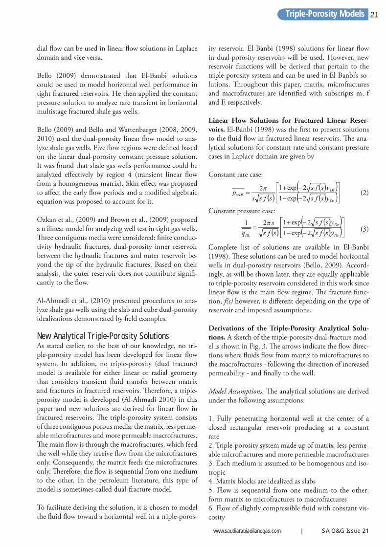
Linear Flow Solutions for Fractured Linear Reser-voirs. El-Banbi (1998) was the fi rst to present solutions to the fl uid fl ow in fractured linear reservoirs. Th e ana-lytical solutions for constant rate and constant pressure cases in Laplace domain are given by
Constant rate case:
(2)
Constant pressure case:
(3)
Complete list of solutions are available in El-Banbi (1998). Th ese solutions can be used to model horizontal wells in dual-porosity reservoirs (Bello, 2009). Accord-ingly, as will be shown later, they are equally applicable to triple-porosity reservoirs considered in this work since linear fl ow is the main fl ow regime. Th e fracture func-tion, f(s) however, is diff erent depending on the type of reservoir and imposed assumptions.
Derivations of the Triple-Porosity Analytical Solu-tions. A sketch of the triple-porosity dual-fracture mod-el is shown in Fig. 3. Th e arrows indicate the fl ow direc-tions where fl uids fl ow from matrix to microfractures to the macrofractures - following the direction of increased permeability - and fi nally to the well.
Model Assumptions. Th e analytical solutions are derived under the following assumptions:
1. Fully penetrating horizontal well at the center of a closed rectangular reservoir producing at a constant rate 2. Triple-porosity system made up of matrix, less perme-able microfractures and more permeable macrofractures 3. Each medium is assumed to be homogenous and iso-tropic 4. Matrix blocks are idealized as slabs 5. Flow is sequential from one medium to the other; form matrix to microfractures to macrofractures 6. Flow of slightly compressible fl uid with constant vis-cosity
Triple-Porosity Models
www.saudiarabiaoilandgas.com | SA O&G Issue 21
21

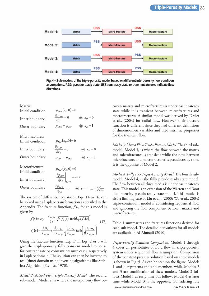
Four Sub-models of the triple-porosity model are derived (Al-Ahmadi, 2010). Th e main diff erence between the models is the assumption of interporosity fl ow condi-tion, i.e., pseudosteady state or transient. Th ese models are shown graphically in Fig. 4. Th e analytical solution derivation for the fully transient (Model 1) is shown in this paper. More detailed solutions derivations for the other models are available in Al-Ahmadi (2010).
Defi nitions of Dimensionless Variables. Before proceeding with the derivations, the dimensionless variables are de-fi ned.
(4)
(5)
(6)
(7)
(8)
(9)
(10)
(11)
(12)
(13)
ω and λ are the storativity ratio and interporosity fl ow parameter, respectively. kF and kf are the bulk (macro-scopic) fractures permeabilities. Detailed parameters defi nitions are available in the nomenclature section in this paper.
Model 1: Fully Transient Triple-Porosity Model. Th e fi rst Sub-model, Model 1, is the fully transient model. Th e fl ow between matrix and microfractures and that be-tween microfractures and macrofractures are under transient condition. Th is model is an extension to the dual-porosity transient slab model (Kazemi 1969 Mod-el). Th e derivation starts by writing the diff erential equa-tions describing the fl ow in each medium.
Matrix:
(14)
Microfractures:
(15)
Macrofractures:
(16)
Th e initial and boundary conditions in dimensionless form are as follows:
Fig. 3 – Top view of a horizontal well in a triple-porosity system with sequential flow. Arrows indicate flow directions (Al-Ahmadi 2010).
Triple-Porosity Models22
Matrix:Initial condition:
Inner boundary:
Outer boundary:
Microfractures:Initial condition:
Inner boundary:
Outer boundary:
Macrofractures:Initial condition:
Inner boundary:
Outer boundary:
Th e system of diff erential equations, Eqs. 14 to 16, can be solved using Laplace transformation as detailed in the Appendix. Th e fracture function, f(s), for this model is given by
(17)
Using the fracture function, Eq. 17 in Eqs. 2 or 3 will give the triple-porosity fully transient model response for constant rate or constant pressure cases, respectively in Laplace domain. Th e solution can then be inverted to real (time) domain using inverting algorithms like Steh-fest Algorithm (Stehfest 1970).
Model 2: Mixed Flow Triple-Porosity Model. Th e second sub-model, Model 2, is where the interporosity fl ow be-
tween matrix and microfractures is under pseudosteady state while it is transient between microfractures and macrofractures. A similar model was derived by Dreier et al., (2004) for radial fl ow. However, their fracture function is diff erent since they had diff erent defi nitions of dimensionless variables and used intrinsic properties for the transient fl ow.
Model 3: Mixed Flow Triple-Porosity Model. Th e third sub-model, Model 3, is where the fl ow between the matrix and microfractures is transient while the fl ow between microfractures and macrofractures is pseudosteady state. It is the opposite of Model 2.
Model 4: Fully PSS Triple-Porosity Model. Th e fourth sub-model, Model 4, is the fully pseudosteady state model. Th e fl ow between all three media is under pseudosteady state. Th is model is an extension of the Warren and Root dual-porosity pseudosteady state model. Th is model is also a limiting case of Liu et al., (2000; Wu et al., 2004) triple-continuum model if considering sequential fl ow and ignoring the fl ow component between matrix and macrofractures.
Table 1 summarizes the fractures functions derived for each sub model. Th e detailed derivations for all models are available in Al-Ahmadi (2010).
Triple-Porosity Solutions Comparison. Models 1 through 4 cover all possibilities of fl uid fl ow in triple-porosity system under sequential fl ow assumption. Comparison of the constant pressure solution based on these models is shown in Fig. 5. As can be seen on the fi gure, Models 1 and 4 represents the end members while Models 2 and 3 are combination of these models. Model 2 fol-lows Model 1 at early time but follows Model 4 at later time while Model 3 is the opposite. Considering rate
Fig. 4 – Sub-models of the triple-porosity model based on different interporosity flow condition assumptions. PSS: pseudosteady state. USS: unsteady state or transient. Arrows indicate flow directions.
Triple-Porosity Models
www.saudiarabiaoilandgas.com | SA O&G Issue 21
23

transient analysis, Models 1 and 3 are more likely to be applicable to fi eld data.
Flow Regions Based on the Analytical Solution. Since Model 1, the fully transient model, is the most gen-eral of all the four triple-porosity variations and shows all possible fl ow regions, the discussions in this paper will be limited to Model 1. Based on Model 1 constant
pressure solution, six fl ow regions can be identifi ed as the pressure propagates through the triple-porosity sys-tem (Al-Ahmadi, 2010). Th ese fl ow regions are shown graphically on the log-log plot of dimensionless rate ver-sus dimensionless time in Fig. 6. Regions 1 through 5 exhibit an alternating slopes of – 1⁄2 and – 1⁄4 indicating linear and bilinear transient fl ow, respectively. Region 6 is the boundary dominated fl ow and exhibits an expo-
Fig. 5 – Comparison of the constant pressure solutions based on the four triple-porosity models assumptions (Al-Ahmadi, 2010).
Triple-Porosity Models24

nential decline due to constant bottom-hole pressure. Th ese fl ow regions are explained in details in the follow-ing sections.
Region 1. Region 1 represents the transient linear fl ow in the macrofractures only. Th e permeability of macrof-ractures is usually high and therefore, in most cases, this fl ow region will be very short. It may not be captured by most well rate measurement tools. Th is fl ow region exhibits a half-slope on the log-log plot of rate versus time.
Region 2. Region 2 is the bilinear fl ow in the macrofrac-tures and microfractures. It is caused by simultaneous perpendicular transient linear fl ow in the microfractures and the macrofractures. Th is fl ow region exhibit a quar-ter-slope on the log-log plot of rate versus time.
Region 3. Region 3 is the linear fl ow in the microfrac-tures system. It will occur once the transient fl ow in the macrofractures ends indicating the end of bilinear fl ow (region 2). Th is fl ow region exhibits a half-slope on the log-log plot of rate versus time.
Region 4. Region 4 is the bilinear fl ow in the microf-
ractures and matrix. It is caused by the linear fl ow in the matrix while the microfractures are still in transient fl ow. Th is fl ow region exhibits a quarter-slope on the log-log plot of rate versus time. In most fi eld cases, this fl ow region is the fi rst one to be observed.
Region 5. Region 5 is the main and longest fl ow region in most fi eld cases. It is the linear fl ow out of the matrix to the surrounding microfractures. Th is region exhibits a half-slope on the log-log plot of rate versus time. Analy-sis of this region will allow the estimation of fractures surface area available to fl ow, Acm.
Region 6. Region 6 is the boundary dominated fl ow. It starts when the pressure at the center of the matrix blocks starts to decline. Th is fl ow is governed by expo-nential decline due to constant bottom-hole pressure.
Model verifi cation Mathematical Consistency of the Analytical Solu-tions. In this section, the solutions mathematical con-sistency is checked by reducing the triple-porosity mod-el to its dual-porosity counterpart. Th is can be achieved by allowing the microfractures to dominate the fl ow and assigning to them the dual-porosity matrix properties
Fig. 6 – A log-log plot of triple-porosity solution. Six flow regions can be identified for Model 1 constant pressure solution. Slopes are labeled on the graph (Al-Ahmadi, 2010).
Triple-Porosity Models
www.saudiarabiaoilandgas.com | SA O&G Issue 21
25

from the dual-porosity system. In this case, the matrix-microfractures interporosity coeffi cient, λAc,fm, is very small and the triple-porosity matrix storativity ratio, ω, is zero.
Th is comparison is shown for all models in the following fi gures. Table 2 shows the data used for comparison.
Models 1 and 2 are reduced to the transient slab dual-porosity model since the fl ow between microfractures and macrofractures is under transient conditions in the two models. Models 3 and 4, however, are reduced to the pseudosteady state dual-porosity model since the fl ow between microfractures and macrofractures is un-der pseudosteady state condition in the two models. As shown in Fig. 7, the triple-porosity solutions are iden-tical to their dual-porosity counterpart. Th is confi rms the mathematical consistency of the new triple-porosity solutions.
Comparison to Simulation Model. A triple-porosity simulation model was built explicitly using CMG res-ervoir simulator to understand the behavior of triple-porosity reservoirs and to verify the derived analytical solutions. Th e model considers the fl ow toward a hori-zontal well in a triple-porosity reservoir. One representa-tive segment is modeled which represents one quadrant of the reservoir volume around a macrofracture. Th is segment contains ten microfractures orthogonal to the macrofractures at 20 ft fracture spacing. Th e model is a 2-D model with 21 gridcells in the x-direction, 211 gridcells in y-direction and only one cell in the z-direc-tion. A top view of the model is shown in Fig. 8. All matrix, microfractures and macrofractures properties are
assigned explicitly. In addition, the simulation model as-sumes constant connate water saturation.
Th e simulation model was run for many cases by chang-ing the three porosities and permeabilities of the three media and the simulation results are compared to that of the analytical solutions for each case. All cases were matched with analytical solutions and thus confi rm-ing their validity. A result of one case for oil reservoir is shown in Fig. 9.
Applicability of Triple-Porosity Solutions for Radial Flow. Although the triple-porosity solutions derived in
Fig. 7 –A log-log plot of transient dual-porosity (DP) and triple-porosity (TP) Models 1 and 2 solutions (on left) and pseudosteady state dual-porosity (DP) and triple-porosity (TP) Models 3 and 4 solutions (on right) for constant pressure linear flow case. In both figures, the two solutions are identical indicating the mathematical consistency of the new triple-porosity solutions.
Fig. 8 – Top view of the CMG 2-D triple-porosity simulation mod-el.
Triple-Porosity Models26

this paper were for linear fl ow, they are equally applica-ble to radial fl ow following El-Banbi (1998) work. Th e diff erential equation in Laplace domain that governs the fl ow in the macrofractures in case of radial system is given by
(18)
Th e constant pressure solution for a closed reservoir is given by (El-Banbi 1998)
(19)
Th e fracture functions, f(s), derived for all the models can be used in the radial fl ow solutions as well. Fig. 10 shows comparison between radial dual-porosity solu-tions and the new triple-porosity solutions reduced to their dual-porosity counterpart and applied to radial fl ow. Data used for comparison are shown in Table 3. Th e solutions are identical indicating the applicability of the new triple-porosity solutions derived in this work to radial fl ow.
Application to Gas Flow. It is important to note that the above solutions were derived for slightly compress-
ible fl uids and thus are applicable to liquid fl ow only. However, they can be applied to gas fl ow by using real gas pseudo-pressure, m(p), instead of pressure to linear-ize the left-hand side of the diff usivity equation. Th ere-fore, the dimensionless pressure variable will be defi ned in terms of real gas pseudo-pressure as:
(20)
where m(p) is the real gas pseudo-pressure defi ned as (Al-Hussainy et al. 1966):
(21)
With the above linearization, the derived solutions are applicable to the transient fl ow regime for gas fl ow.
However, once the reservoir boundaries are reached and average reservoir pressure starts to decline, the gas prop-erties will change considerably especially the gas viscos-ity and compressibility. Th erefore, the solutions have to be corrected for changing fl uid properties. Th is is usu-ally achieved by using pseudo-time or material balance time. An example of these transformations is the Fraim and Wattenbarger (1987) normalized time defi ned as
Fig. 9 – Match between simulation and analytical solution results for oil reservoir case. (kF,in = 1000 md, kf,in = 1 md and km = 1.5×10 md) (Al-Ahmadi 2010).
Triple-Porosity Models
www.saudiarabiaoilandgas.com | SA O&G Issue 21
27

(22)
Th us, with these two modifi cations, the analytical solu-tions derived in this work are applicable to gas fl ow.
Accounting for Adsorbed Gas. Unlike tight gas reser-voirs, gas in shale reservoirs is stored as compressed (free) gas and adsorbed gas. Adsorbed gas does not usually fl ow until the pressure drops below the sorption pres-sure. Adsorbed gas can be accounted for using Langmuir isotherm which defi nes the adsorbed gas volume as:
(23)
where
V: Volume of gas currently adsorbed (scf/cuf ) VL: Langmuir’s volume (scf/cuf ) pL: Langmuir’s pressure (psia) pLp: Reservoir pressure (psia)
Th erefore, the analytical solutions have to account for the adsorbed gas before applying them to shale gas wells. Th is can be achieved by modifying the gas compressibil-ity defi nition to include adsorbed gas. Following Bumb and McKee (1988), the modifi ed total compressibility is defi ned as:
(24)
where cd is the desorbed gas compressibility given by:
(25)
Th us, to account for adsorption, c*t instead of ct will be
used in the analytical solutions to be applicable to shale gas wells.
For material balance calculations, the modifi ed com-pressibility factor (z*) is used instead of z (King 1993). z* is defi ned as:
(26)
Th en the gas material balance equation becomes:
(27)
Th e OGIP accounting for free and adsorbed gas can be calculated using the following volumetric equation (Sa-mandarli 2011):
(28)
Field Application Tight reservoirs such as shale oil or shale gas are perfect fi eld case to apply this model due to the large contrast in the three porous media permeability values. Horizontal wells placed in these reservoirs are usually hydraulically fractured due to low matrix permeability. Natural frac-tures usually exist in these reservoirs as well. Th e case presented here is from a shale gas reservoir.
Shale Gas reservoirs play a major role in the United State natural gas supply as they are aggressively devel-oped capitalizing on new technologies, namely horizon-tal wells with multistage fracturing. It has been observed that these wells behave as though they are controlled by transient linear fl ow (Bello 2009; Bello and Wat-tenbarger 2008, 2009, 2010; Al-Ahmadi et al., 2010). According to Medeiros et al., (2008) linear fl ow is the
Fig. 10 – Log-log plot of dual-porosity and triple-porosity constant pressure solutions for radial flow. On the left is the transient solution and on right is the pseudosteady solution (Al-Ahmadi 2010).
Triple-Porosity Models28

dominant fl ow regime for fractured horizontal wells in tight formations for most of their productive lives. Th is behavior is characterized by a negative half-slope on the log-log plot of gas rate versus time and a straight line on the [m(pi) – m(pwf)]/qg vs. t0.5 plot (the square root of time plot).
Some shale gas wells, however, exhibit a bi-linear fl ow just before the linear fl ow is observed. Th is behavior is characterized by a negative quarter-slope on the log-log plot of gas rate versus time or a straight line on the [m(pi) – m(pwf)]/qg vs. t0.25 plot. Th e bi-linear fl ow is due to two perpendicular transient linear fl ows occurring si-multaneously in two contiguous systems. Th ese could be microfractures and matrix or microfractures and macrofractures systems.
Previously, shale gas wells have been modeled using line-ar dual-porosity models (Bello 2009; Bello and Watten-barger 2008, 2009, 2010; Al-Ahmadi et al., 2010). In these models, the matrix was assumed “homogeneous” although it might be enhanced by natural fractures by having high eff ective matrix permeability. In addition, orthogonal fractures are assumed to have identical prop-erties. However, most if not all of horizontal wells drilled in shale gas reservoirs are hydraulically fractured. As the hydraulic fractures propagate, they re-activate the pre-existing natural fractures (Gale et al., 2007). Th e result will be two orthogonal fractures systems with diff erent properties. Th erefore, dual porosity model will not be suffi cient to characterize these reservoirs. As a result, the triple-porosity model with fully transient fl ow assump-tion (Model 1) will be used to model horizontal shale gas wells. For this specifi c case, macrofractures are the hydraulic fractures while microfractures are the natural fractures.
Analysis Procedure. Due to the large number of vari-ables involved in the triple-porosity model, nonlinear regression will be utilized to estimate a set of unknown parameters by matching the well’s production rate. Other parameters may be assumed or estimated through other methods. Including many variables in the regres-sion may lead to non-uniqueness of the converged solu-tion. Th e parameters to be found by regression are frac-tures intrinsic permeabilities, drainage area half-width (hydraulic fracture half-length) and natural fractures spacing. After the match is obtained, the well model is fully defi ned. Hence, the OGIP can be calculated by volumetric method and well future production can be forecasted.
Nonlinear Regression. Th e triple-porosity model
presented in this paper needs at most fi ve parameters; namely two ω’s, two λ’s and yDe. In addition, these calcu-lated parameters depend on reservoir properties which have to be estimated. Th is leads to estimation of many parameters that may not be known or needs to be calcu-lated. Th erefore, the need for regression arises in order to match fi eld data and have a good estimate of the sought reservoir or well parameters. In automated well test in-terpretations, the common regression methods are the least squares (LS), least absolute value (LAV) and modi-fi ed least absolute value minimization (Rosa and Horne 1995, 1996). It was found, however, that the least ab-solute value regression method is the most appropriate in matching noisy data and can be used eff ectively with triple-porosity model to match fi eld data (Al-Ahmadi 2010).
However, in order to get the most accurate results with regression, data that shows special trends should be in-cluded in the regression. For example, if the data that shows linear fl ow was only included in the regression and the data that shows a bi-linear fl ow just before it was ignored, the data will be matched but the solutions will not be representative as if that data was also included. In short, as expected the more data included in the regres-sion, the more accurate the results will be.
Field Case. A fi eld case from the Barnett Shale will be used to demonstrate the application of the triple-poros-ity model. Gas rate history for these wells is shown in Fig. 11. Th e fully transient model (Model 1) with non-linear regression and normalized time will be applied. Gas adsorption will be included in the analysis as well. Th e well is matched with the analytical solutions by fi rst assuming no adsorbed gas and then including gas ad-sorption. Comparisons are made for each well. Th e fol-lowing adsorption data are used for the Barnett Shale (Mengal 2010):
VL = 96 scf/ton pL = 650 psi Bulk Density = 2.58 gm/cc
Well 314 is a horizontal well with multistage hydraulic fracturing treatment producing at a constant bottom-hole pressure.
Th e well production rate exhibits a half-slope on the log-log plot of rate versus time indicating a linear fl ow. However, the early and late data deviate from this trend. Th e early deviation may be due to skin eff ect due to the presence of fracturing job water in the hydraulic frac-tures making it diffi cult for the gas to start fl owing to
Triple-Porosity Models
www.saudiarabiaoilandgas.com | SA O&G Issue 21
29

the well (Bello and Wattenbarger 2009; Al-Ahmadi et al., 2010). Th e later deviation is due to either start of boundary dominated fl ow (BDF) or reduction of well’s drainage area due to drilling nearby well. In this work, no skin eff ect is considered and the later deviation will be dealt with as BDF. However, if the well is aff ected by skin, it results in a lower permeability value for the hydraulic fractures.
Table 4 summarizes well 314 data in addition to other assumed parameters. From the hydraulic fractures treat-ment, hydraulic fractures spacing is calculated assum-ing each perforation cluster corresponds to a hydraulic fracture. In addition, drainage area length, xe, is the same
as perforated interval. Th e matrix porosity and perme-ability used are the most available in the literature for the Barnett Shale. Representative values are assumed for fractures intrinsic porosity and width. Finally, the frac-tures intrinsic permeabilities, drainage area half-width and natural fractures spacing will be found by regres-sion.
Regression results are shown in Table 5 and Fig. 12 with and without adsorption using LAV method.
From the regression results above, the hydraulic frac-tures intrinsic permeability is more than an order of magnitude compared to that of the natural fractures.
Fig. 11 – Log-Log plot of gas rate versus time for a hori-zontal shale gas wells. The well exhibits a linear flow for almost two log cycles. The blue and indicates a half-slope.
Triple-Porosity Models30

In addition, the natural fractures permeability is about three orders of magnitude compared to the matrix per-meability. Furthermore, the natural fracture spacing is about 23 ft indicating that matrix is in fact enhanced by natural fractures.
Including adsorption did not change the estimate of fractures intrinsic permeabilities or the natural fractures spacing but it had a big impact on drainage area half-width and consequently OGIP. Th us, including adsorp-
tion reduces the reservoir size while increasing its gas content by 35%. Th e same matrix porosity was used in both cases which may not be physically correct. Th e calculated OGIP is 3.01 Bscf if adsorbed gas is ignored. Al-Ahmadi et al., (2010) estimated 2.74 Bscf for OGIP for this well using linear dual-porosity model. Th e two estimates are within 10% relative error.
Knowing all the triple-porosity parameters, the whole well production history is forecasted as shown in Fig.
Fig. 12 – Matching Well 314 production history using the regression results without (top) and with (bottom) adsorption. On the left is the decline curve plot and log-log plot is on the right for gas rate vs. time.
Triple-Porosity Models
www.saudiarabiaoilandgas.com | SA O&G Issue 21
31
12 based on the regression results for the fi rst 500 days. As can be seen, the model very well reproduced the well production trend with and without adsorption as shown on the log-log and decline curve plots.
Conclusions Th e major conclusions from this work can be summa-rized as follows:
1. Triple-porosity models are proposed as a more practi-cal technique for capturing fractured reservoir heteroge-neity by allowing fractures to have diff erent properties. 2. New triple-porosity (dual-fracture) solutions have been developed for fractured linear reservoirs and proved to be applicable to radial fl ow geometry as well. 3. Six fl ow regions can be identifi ed for fully transient triple-porosity model (Model 1). 4. Th e new model has been verifi ed by reducing it to simpler dual porosity models and by comparing it to reservoir simulation. 5. Th e derived solutions are also applicable to gas fl ow using gas real gas pseudo-pressure and normalized time. 6. Triple-porosity fully transient model (Model 1) is ap-plicable to fractured shale gas horizontal wells when gas adsorption is incorporated. Th e model can be used to match fi eld data, characterize well drainage area, deter-mine reservoir size and OGIP and forecast future pro-duction.
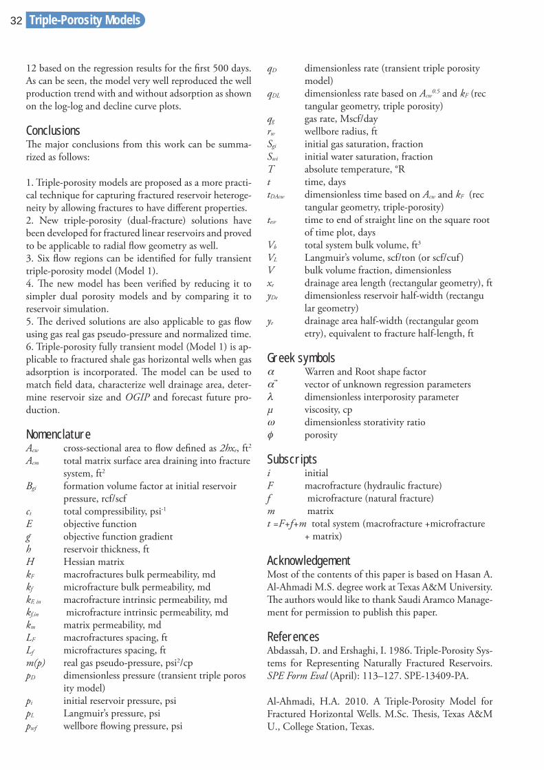
Nomenclature Acw cross-sectional area to fl ow defi ned as 2hxe, ft2 Acm total matrix surface area draining into fracture system, ft2
Bgi formation volume factor at initial reservoir pressure, rcf/scfct total compressibility, psi-1 E objective function g- objective function gradient h reservoir thickness, ft H Hessian matrix kF macrofractures bulk permeability, md kf microfracture bulk permeability, md kF, in macrofracture intrinsic permeability, md kf,in microfracture intrinsic permeability, md km matrix permeability, md LF macrofractures spacing, ft Lf microfractures spacing, ft m(p) real gas pseudo-pressure, psi2/cp pD dimensionless pressure (transient triple poros ity model) pi initial reservoir pressure, psi pL Langmuir’s pressure, psi pwf wellbore fl owing pressure, psi
qD dimensionless rate (transient triple porosity model) qDL dimensionless rate based on Acw
0.5 and kF (rec tangular geometry, triple porosity) qg gas rate, Mscf/day rw wellbore radius, ft Sgi initial gas saturation, fraction Swi initial water saturation, fraction T absolute temperature, °R t time, days tDAcw dimensionless time based on Acw and kF (rec tangular geometry, triple-porosity) tesr time to end of straight line on the square root of time plot, days Vb total system bulk volume, ft3 VL Langmuir’s volume, scf/ton (or scf/cuf ) V bulk volume fraction, dimensionless xe drainage area length (rectangular geometry), ft yDe dimensionless reservoir half-width (rectangu lar geometry) ye drainage area half-width (rectangular geom etry), equivalent to fracture half-length, ft
Greek symbols α Warren and Root shape factor α� vector of unknown regression parameters λ dimensionless interporosity parameter μ viscosity, cp ω dimensionless storativity ratio φ porosity
Subscripts i initial F macrofracture (hydraulic fracture) f microfracture (natural fracture) m matrix t =F+f+m total system (macrofracture +microfracture + matrix)
Acknowledgement Most of the contents of this paper is based on Hasan A. Al-Ahmadi M.S. degree work at Texas A&M University. Th e authors would like to thank Saudi Aramco Manage-ment for permission to publish this paper.
References Abdassah, D. and Ershaghi, I. 1986. Triple-Porosity Sys-tems for Representing Naturally Fractured Reservoirs. SPE Form Eval (April): 113–127. SPE-13409-PA.
Al-Ahmadi, H.A. 2010. A Triple-Porosity Model for Fractured Horizontal Wells. M.Sc. Th esis, Texas A&M U., College Station, Texas.
Triple-Porosity Models32

Al-Ahmadi, H.A., Almarzooq, A.M. and Wattenbarger, R.A. 2010. Application of Linear Flow Analysis to Shale Gas Wells – Field Cases. Paper SPE 130370 presented at the 2010 Unconventional Gas Conference, Pittsburgh, Pennsylvania, 23-25 February.
Al-Ghamdi, A. and Ershaghi, I. 1996. Pressure Transient Analysis of Dually Fractured Reservoirs. SPE J. (March): 93–100. SPE-26959-PA.
Al-Hussainy, R., Ramey Jr., H.J. and Crawford, P.B. 1966. Th e Flow of Real Gas Th rough Porous Media. J. Pet Tech (May): 624–636. SPE-1243A-PA
Anderson, D.M., Nobakht, M., Moghadam, S. and Mattar, L. 2010. Analysis of Production Data from Fractured Shale Gas Wells. Paper SPE 131787 presented at the SPE Unconventional Gas Conference, Pittsburgh, Pennsylvania, 23-25 February.
Barenblatt, G.I., Zhelto, I.P. and Kochina, I.N. 1960. Basic Concepts of the Th eory of Seepage of Homogene-ous Liquids in Fissured Rocks. Journal of Applied Math-ematical Mechanics (USSR) 24 (5): 852–864.
Barrodale, I. and Roberts, F.D.K. 1974. Solution of an Overdetermined System of Equations in the l1 Norm. Communication of the ACM 17 (6): 319–320.
Bello, R.O. and Wattenbarger, R.A. 2008. Rate Tran-sient Analysis in Naturally Fractured Shale Gas Reser-voirs. Paper SPE 114591 presented at the CIPC/SPE Gas Technology Symposium 2008 Joint Conference, Calgary, Alberta, Canada, 16-19 June.
Bello, R.O. and Wattenbarger, R.A. 2009. Modeling and Analysis of Shale Gas Production with a Skin Ef-fect. Paper CIPC 2009-082 presented at the Canadian International Petroleum Conference, Calgary, Alberta, Canada, 16-18 June.
Bello, R.O. and Wattenbarger, R.A. 2010. Multistage Hydraulically Fractured Shale Gas Rate Transient Anal-ysis. Paper SPE 126754 presented at the SPE North Af-rica Technical Conference and Exhibition held in Cairo, Egypt, 14-17 February.
Bello, R.O. 2009. Rate Transient Analysis in Shale Gas Reservoirs with Transient Linear Behavior. Ph.D. Dis-sertation, Texas A&M U., College Station, Texas.
Brown, M., Ozkan, E., Raghavan, R. and Kazemi, H. 2009. Practical Solutions for Pressure Transient Re-
sponses of Fractured Horizontal Wells in Unconven-tional Reservoirs. Paper SPE 125043 presented at the Annual Technical Conference and Exhibition, New Or-leans, Louisiana, 4-7 October.
Bumb, A.C. and McKee, C.R. 1988. Gas-Well Test-ing in the Pressure of Desorption for Coalbed Methane and Devonian Shale. SPE Form Eval (March): 179-185. SPE-15227-PA.
Cheney, E.W. and Kincaid, R.D. 1985. Numerical Mathematics and Computing, 2nd edition. Monterey, California: Brooks/Cole Publishing Company.
CMG Simulator. 2008. Computer Modeling Group, Calgary, Canada.
de Swaan, O.A. 1976. Analytic Solutions for Determin-ing Naturally Fractured Reservoir Properties by Well Testing. SPE J. (June): 117– 122. SPE-5346-PA.
Dreier, J. 2004. Pressure-Transient Analysis of Wells in Reservoirs with a Multiple Fracture Network. M.Sc. Th esis, Colorado School of Mines, Golden, Colorado.
Dreier, J., Ozkan, E. and Kazemi, H. 2004. New Ana-lytical Pressure-Transient Models to Detect and Charac-terize Reservoirs with Multiple Fracture Systems. Paper SPE 92039 presented at the SPE International Petro-leum Conference in Mexico, Puebla, Mexico, 8-9 No-vember.
El-Banbi, A.H. 1998. Analysis of Tight Gas Wells. Ph.D. Dissertation, Texas A&M U., College Station, Texas.
Fraim, M.L. and Wattenbarger, R.A. 1987. Gas Res-ervoir Decline-Curve Analysis Using Type Curve with Real Gas Pseudopressure and Normalized Time. SPE Form Eval (December): 671–682. SPE-14238-PA.
Gale, J.F., Reed, R.M. and Holder, J. 2007. Natural Fractures in the Barnett Shale and their Importance for Hydraulic Fracture Treatments. AAPG Bulletin. 91 (4): 603–622.
Jalali, Y. and Ershaghi, I. 1987. Pressure Transient Anal-ysis of Heterogeneous Naturally Fractured Reservoirs. Paper SPE 16341 presented at the SPE California Re-gional Meeting, Ventura, California, 8-10 April.
Kazemi, H. 1969. Pressure Transient of Naturally Frac-tured Reservoirs with Uniform Fracture Distribution. SPE J. (December):451–462. SPE-2156A-PA.
Triple-Porosity Models
www.saudiarabiaoilandgas.com | SA O&G Issue 21
33

King, G.R. 1993. Material-Balance Techniques for Coal-Seam and Devonian Shale Gas Reservoirs with Limited Water Infl ux. SPE Res Eng (February): 67–72. SPE-20730-PA.
Liu, C.Q. 1981. Exact Solution for the Compressible Flow Equations through a Medium with Triple-Porosity. Applied Mathematics and Mechanics 2 (4): 457–462.
Liu, C.Q. 1983. Exact Solution of Unsteady Axisym-metrical Two-Dimensional Flow through Triple Porous Media. Applied Mathematics and Mechanics 4 (5): 717–724.
Liu, J.C., Bodvarsson, G.S. and Wu, Y.S. 2003. Analysis of Flow Behavior in Fractured Lithophysal Reservoirs. Journal of Contaminant Hydrology 62-63: 189–211.
Mayerhofer, M.J., Lolon, E.P., Youngblood, J.E. and Heinze, J.R. 2006. Integration of Microseismic Fracture Mapping Results with Numerical Fracture Network Production Modeling in the Barnett Shale. Paper SPE 102103 presented at the Annual Technical Conference and Exhibition, San Antonio, Texas, 24-27 September.
Medeiros, F., Ozkan, E. and Kazemi, H. 2008. Produc-tivity and Drainage Area of Fractured Horizontal Wells in Tight Gas Reservoirs. SPE Res Eval & Eng (October): 902–911. SPE-108110-PA.
Mengal, S.A. 2010. Accounting for Adsorbed Gas and
Its Eff ect on Production Behavior of Shale Gas Reser-voirs. M.Sc. Th esis, Texas A&M U., College Station, Texas.
Nelson, R.A. 2001. Geologic Analysis of Naturally Frac-tured Reservoirs, 2nd edition. Woburn, Massachusetts: Butterworth-Heinemann.
Ozkan, E., Brown, M., Raghavan, R. and Kazemi, H. 2009. Comparison of Fractured Horizontal-Well Per-formance in Conventional and Unconventional Reser-voirs. Paper SPE 121290 presented at the SPE Western Regional Meeting, San Jose, California, 24-26 March.
Ozkan, E., Ohaeri, U. and Raghavan, R. 1987. Un-steady Flow to a Well Produced at a Constant Pressure in Fractured Reservoir. SPE Form Eval (June): 186-200. SPE-9902-PA.
Rosa, A.J. and Horne, R.N. 1995. Automated Well Test Analysis Using Robust (LAV) Nonlinear Parameter Es-timation. SPE Advanced Technology Series 3 (1): 95–102. SPE-22679-PA.
Rosa, A.J. and Horne, R.N. 1996. New Approaches for Robust Nonlinear Parameter Estimation in Automated Well Test Analysis Using the Least Absolute Value Crite-rion. SPE Advanced Technology Series 4 (1): 21–27. SPE-26964-PA.
Samandarli, O. 2011. A New Method for History
Fig. A-1 – A sketch of triple-porosity system under sequential feed assumption. Ar-rows show flow directions.
Triple-Porosity Models34

Matching and Forecasting of Shale Gas/Oil Reservoirs with Dual and Triple-Porosity Systems. M.Sc. Th esis, Texas A&M U., College Station, Texas.
Sarma, P. and Aziz, K. 2006. New Transfer Functions for Simulation of Naturally Fractured Reservoirs with Dual-Porosity Models. SPE J. (September): 328–340. SPE-90231-PA.
Stehfest, H. 1970. Algorithm 358 – Numerical Inver-sion of Laplace Transforms. Communication of the ACM 13 (1): 47 – 49.
Van Everdingen, A.F. and Hurst, W. 1949. Th e Applica-tion of the Laplace Transformation to Flow Problems in Reservoirs. Trans., AIME, 186: 305–324.
Warren, J.E. and Root, P.J. 1963. Th e Behavior of Natu-rally Fractured Reservoirs. SPE J. (September): 245–255. SPE-426-PA.
Wattenbarger, R.A. 2007. Some Reservoir Performance Aspects of Unconventional Gas Production. Private Conference Presentation.
Wu, Y.S., Liu, H.H. and Bodvarsson, G.S. 2004. A Triple-Continuum Approach for Modeling Flow and Transport Processes in Fractured Rock. Journal of Con-taminant Hydrology 73: 145–179.
Appendix: Derivation of Linear Triple-Porosity Fully Transient Model Model 1: Fully Transient Triple-Porosity Model. Th e fi rst Sub-model, Model 1, is the fully transient model. Th e fl ow between matrix and microfractures and that be-tween microfractures and macrofractures are under transient condition. Th is model is an extension to the dual-porosity transient slab model (Kazemi 1969 Mod-el). Th e derivation starts by writing the diff erential equa-tions describing the fl ow in each medium.
Matrix Equation Since the fl ow transfer from matrix to fractures is under transient condition, the matrix equation is given by:
(A-1)
Note: z here is a direction parallel to y-axis. It is not the vertical direction. Microfracture Equation
(A-2)
qsource,m , is a source term of fl ow from matrix to the mi-
crofracture under transient fl ow and can be written as:
(A-3)
Th us, the fi nal form of microfractures equation is:
(A-4)
Macrofracture Equation Th e macrofractures receive fl ow from the microfrac-tures and the fl ow can be modeled using the equation:
(A-5)
qsource,f , is the source term of fl ow from microfractures to the macrofracture under transient fl ow and can be written as:
(A-6)
Th us, the fi nal form of microfractures equation is:
(A-7)
System of Equations with Initial and Boundary Conditions
Matrix:
(A-1)
Microfractures:
(A-4)
Macrofractures:
(A-7)
Initial and boundary conditions are:
Matrix:
Initial condition:
Inner boundary:
Outer boundary:
Microfractures:
Initial condition:
Triple-Porosity Models
www.saudiarabiaoilandgas.com | SA O&G Issue 21
35

Inner boundary:
Outer boundary:
Macrofractures:
Initial condition:
Inner boundary:
Outer boundary:
System Dimensionless Equations with Initial and Boundary Conditions
Matrix:
(A-8)
Microfractures:
(A-9)
Macrofractures:
(A-10)
Dimensionless initial and boundary conditions are:
Matrix:
Initial condition:
Inner boundary:
Outer boundary:
Microfractures:
Initial condition:
Inner boundary:
Outer boundary:
Macrofractures:
Initial condition:
Inner boundary:
Outer boundary:
Laplace Transformation
In order to solve the above system of diff erential equa-tions, they have to be transformed into Laplace domain for easier solving as detailed below.
Matrix equation:
(A-11)
Th e initial and boundary conditions in Laplace domain are:
Initial condition:
Inner boundary:
Outer boundary:
Using the initial condition, Eq. A-11 becomes:
(A-12)
Th e general solution for Eq. A-12 is given by:
(A-13)
Th e constants A and B are determined as:
(A-14)
(A-15)
Th erefore, the fi nal solution for Eq. A-12 is
(A-16)
Microfractures equation:
(A-17)
Th e initial and boundary conditions in Laplace domain are:
Initial condition:
Inner boundary:
Outer boundary:
Triple-Porosity Models36

Using the initial condition, Eq. A-17 becomes:
(A-18)
Now, diff erentiating Eq. A-16, we have:
(A-19)
Substituting Eq. A-19 in A-18:
(A-20)
Or in short form:
(A-21)
where
(A-22)
Th e general solution for Eq. A-21 is given by:
(A-23)
Th e constants A and B are determined as:
B = 0 (A-24)
(A-25)
Th erefore, the fi nal solution for Eq. A-21 is:
(A-26)
Macrofractures equation:
(A-27)
Initial and boundary conditions in Laplace domain are:
Initial condition:
Inner boundary:
Outer boundary:
Using the initial condition, Eq. A-27 becomes:
(A-28)
Now diff erentiating Eq. A-26:
. (A-29)
Now Eq.A-28 becomes:
(A-30)
Or in short form:
(A-31)
where f(s) is the defi nition for the fracture function for Model 1:
(A-32)
Using this fracture function in Eqs. 2 or 3 will give the triple-porosity fully transient response for constant rate or constant pressure cases, respectively.
Detailed derivations of the other three models are avail-able in Al-Ahmadi (2010).
Triple-Porosity Models
www.saudiarabiaoilandgas.com | SA O&G Issue 21
37

Surfactant-Polymer Flood Performance38
By Nawaf I. SayedAkram, Saudi Aramco; Daulat Mamora,Texas A&M University.
Copyright 2011, Society of Petroleum Engineers
This paper was prepared for presentation at the 2011 SPE Saudi Arabia Section Technical Symposium and Exhibition held in AlKhobar, Saudi Arabia, 15–18 May 2011.
This paper was selected for presentation by an SPE program committee following review of information contained in an abstract submit-ted by the author(s). Contents of the paper have not been reviewed by the Society of Petroleum Engineers and are subject to correction by the author(s). The material, as presented, does not necessarily reflect any position of the Society of Petroleum Engineers, its officers, or members. Papers presented at the SPE meetings are subject to publication review by Editorial Committee of Society of Petroleum Engineers. Electronic reproduction, distribution, or storage of any part of this paper without the written consent of the Society of Petroleum Engineers is prohibited. Permission to reproduce in print is restricted to an abstract of not more than 300 words; illustrations may not be copied. The abstract must contain conspicuous acknowledgment of where and whom the paper was presented. Write Liberian, SPE, P.O. Box 833836, Richardson, TX 75083-3836, U.S.A., fax 01-972-952-9435.
Simulation Study on Surfactant-Polymer Flood Performance in Fractured Carbonate Reservoir
Abstract Th is paper presents a comprehensive simulation study on the impact of natural fractures on the performance of surfactant polymer fl ood in a fi eld wide scale. Th e simu-lation model utilized for the study is a dual porosity dual permeability model representing 1/8 of a 20-acre 5-spot pattern. Th e model parameters studied include wettabil-ity alteration, interfacial-tension changes and mobility reduction eff ect. Th e results of this study clearly indi-cate the importance of reservoir description and fracture modeling for a successful surfactant-polymer fl ood. Th is may lead in huge diff erence in reserves booking from such EOR method.
Naturally fractured carbonate reservoirs are usually characterized by mixed wettablility and low matrix per-meability which leads to low oil recovery and high re-maining oil saturation. Enhanced oil recovery methods
such as surfactant-polymer fl ood (SPF) enhance the re-covery by increasing the spontaneous imbibitions either by lowering the interfacial tension or altering the wet-tability in the matrix. However, one of the main reasons for failed surfactant-polymer fl oods is under-estimating the importance of the reservoir and fl uid characteristics especially the description of natural fractures and their eff ect on recovery.
Sensitivity runs were made in fi eld size scale in order to compare oil recovery by capillary force, buoyancy force and viscous force. Th e simulation study indicates a re-lationship between water saturation and the start of al-tering wettability and/or interfacial tension to maximize oil recovery. Also, when a surfactant alters the rock wet-tability, an optimum IFT should be identifi ed for faster and higher imbibitions. In addition, the study shows ef-fect on recovery by permeability contrast between that

Surfactant-Polymer Flood Performance
www.saudiarabiaoilandgas.com | SA O&G Issue 21
39
of the fracture and that of the matrix as well as fracture orientation with respect to injector-producer direction.
Introduction About 40-60% of the original oil-in-place (OOIP) in reservoirs is left behind after secondary recovery. Over 60% of the remaining oil in the world can be found in carbonate reservoirs, which makes it a big area of inter-est for Enhance Oil Recovery (EOR) methods especially with the current oil price and increasing demand. Most of the carbonate reservoirs are fractured to a certain de-gree and either oil-wet or mixed-wet (Mohan, 2009).
Th e main characteristics of fractured reservoirs are the permeability enhancement provided by the fractures. In tight matrix blocks, fractures are the only means of fl uid fl ow into a production well. However, the heterogeneity between fractures and matrix blocks can result in by-passed oil.
Chemical EOR Chemical EOR is becoming more attractive with the current economics especially for water fl ooded reser-voirs. Chemical EOR utilizes surfactant, polymers, al-kaline agents or combination of these chemicals (Th o-mas, 2006). Th e use of the surfactant is either to:
• lower the interfacial tension IFT between the hydro-carbon and the injected fl uid, • create macro or micro-emulsions with oil and water that leads to improved sweep effi ciency, • change wettability to water wet through adsorption in the rock formation, or • combination of the above.
A polymer is usually added to the injected water to en-hance sweep effi ciency by decreasing the mobility or in-creasing viscosity of the displacing fl uid. Performance prediction of chemical EOR - such as surfactant-pol-ymer fl ooding - in naturally fractured reservoirs is es-sential for pilot testing, fi eld wide implementation and reservoir management. Generally, recovery prediction continues to be a challenging topic in fractured reser-voirs. Not having a good simulation model that can cap-ture all the interaction of the additives injected in the fractured reservoir can lead to a faulty estimation of fi eld performance or wrong pilot design.
Th e main objective of this work is to study the eff ect of natural fractures on surfactant polymer fl ood (SPF) per-formance on a fi eld scale using a dual-porosity dual-per-meability (DPDP) simulation model. Th e parameters to be studied will include:
fracture permeability, spacing and orientation, matrix permeability and wettability, and the use of low inter-facial tension versus capillary pressure for recovery. Th e main performance measurements used in this study are oil recovery with respect to the original oil-in-place (OOIP).
SOR Reduction Interfacial tension (IFT) reduction plays a signifi cant role in reducing the residual oil saturation (Sor). Taber (1969) found that, in order for a water fl ood to have ef-fect on Sor reduction from the reservoir, interfacial ten-sion must be lowered by a factor of 1,000 or more. IFT is generally hard to be measured in the fi eld due to the high sensitivity to temperature, pressure and presence of
Fig. 1___Spontaneous imbibition through buoyancy force (Hirasaki and Zhang, 2004).
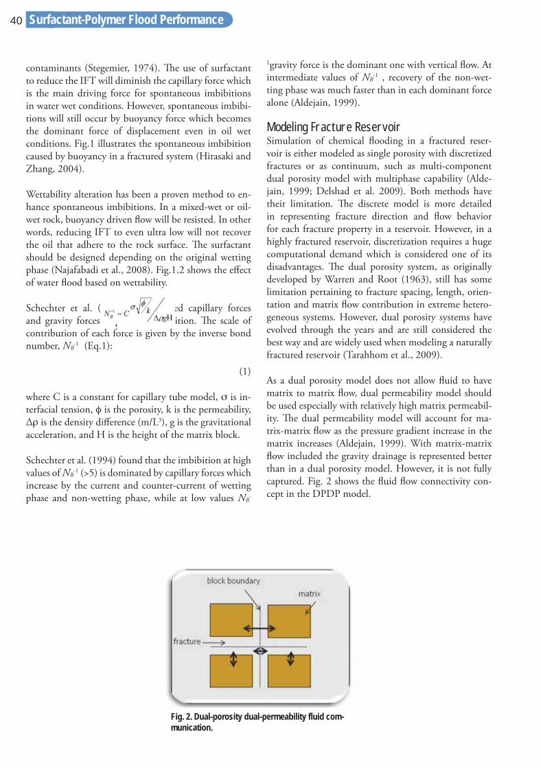
Surfactant-Polymer Flood Performance40
contaminants (Stegemier, 1974). Th e use of surfactant to reduce the IFT will diminish the capillary force which is the main driving force for spontaneous imbibitions in water wet conditions. However, spontaneous imbibi-tions will still occur by buoyancy force which becomes the dominant force of displacement even in oil wet conditions. Fig.1 illustrates the spontaneous imbibition caused by buoyancy in a fractured system (Hirasaki and Zhang, 2004).
Wettability alteration has been a proven method to en-hance spontaneous imbibitions. In a mixed-wet or oil-wet rock, buoyancy driven fl ow will be resisted. In other words, reducing IFT to even ultra low will not recover the oil that adhere to the rock surface. Th e surfactant should be designed depending on the original wetting phase (Najafabadi et al., 2008). Fig.1.2 shows the eff ect of water fl ood based on wettability.
Schechter et al. (1991) have studied capillary forces and gravity forces impact on imbibition. Th e scale of contribution of each force is given by the inverse bond number, NB
-1 (Eq.1):
(1)
where C is a constant for capillary tube model, σ is in-terfacial tension, φ is the porosity, k is the permeability, Δρ is the density diff erence (m/L3), g is the gravitational acceleration, and H is the height of the matrix block.
Schechter et al. (1994) found that the imbibition at high values of NB
-1 (>5) is dominated by capillary forces which increase by the current and counter-current of wetting phase and non-wetting phase, while at low values NB
-
1gravity force is the dominant one with vertical fl ow. At intermediate values of NB
-1 , recovery of the non-wet-ting phase was much faster than in each dominant force alone (Aldejain, 1999).
Modeling Fracture Reservoir Simulation of chemical fl ooding in a fractured reser-voir is either modeled as single porosity with discretized fractures or as continuum, such as multi-component dual porosity model with multiphase capability (Alde-jain, 1999; Delshad et al. 2009). Both methods have their limitation. Th e discrete model is more detailed in representing fracture direction and fl ow behavior for each fracture property in a reservoir. However, in a highly fractured reservoir, discretization requires a huge computational demand which is considered one of its disadvantages. Th e dual porosity system, as originally developed by Warren and Root (1963), still has some limitation pertaining to fracture spacing, length, orien-tation and matrix fl ow contribution in extreme hetero-geneous systems. However, dual porosity systems have evolved through the years and are still considered the best way and are widely used when modeling a naturally fractured reservoir (Tarahhom et al., 2009).
As a dual porosity model does not allow fl uid to have matrix to matrix fl ow, dual permeability model should be used especially with relatively high matrix permeabil-ity. Th e dual permeability model will account for ma-trix-matrix fl ow as the pressure gradient increase in the matrix increases (Aldejain, 1999). With matrix-matrix fl ow included the gravity drainage is represented better than in a dual porosity model. However, it is not fully captured. Fig. 2 shows the fl uid fl ow connectivity con-cept in the DPDP model.
Fig. 2. Dual-porosity dual-permeability fluid com-munication.

Surfactant-Polymer Flood Performance
www.saudiarabiaoilandgas.com | SA O&G Issue 21
41
Approach To achieve the research objective a hypothetical naturally fractured reservoir model has been built. A commercial simulator, CMG Stars version 2009.1, has been utilized which has the capability to simulate chemical EOR processes. Th e study involved the following steps.
• Build a 1/8 model of an inverted 5-spot pattern to simulate a surfactant-polymer fl ood in a carbonate light oil reservoir (black-oil model). • Include dual-permeability dual-porosity (DPDP) mod-el to capture the eff ect of fracture system in the fi eld. • Add rock and fl uid parameters based on published data that represent a common carbonate reservoir from permeability and porosity to wettability conditions and capillary pressure.
• Assume that surfactant used has impact on both wet-tability alteration and IFT reduction while the polymer changes viscosity of the injected fl uid. • Run sensitivity study on surfactant polymer fl ooding (SPF) performance with respect to the start of the proc-ess and the length of the injection through the life of the fi eld. • Run a sensitivity study on fracture spacing, permeabil-ity, fl ow direction, and matrix permeability.
Model Construction Th e reservoir is assumed to be a fractured carbonate res-ervoir characterized by high fracture fl ow and low matrix fl ow. Because matrix to matrix fl ow was not neglected, dual-porosity dual-permeability (DPDP) model was used to capture this fl ow behavior. Th e simulation study
Fig. 3. Plan view and 3D view of the simulation model representing 1/8 of a 20-ac 5-spot pattern.

Surfactant-Polymer Flood Performance42
was done using a commercial simulator, CMG STARS 2009. A 16 x 31 x 5 Cartesian grid model has been used to represent a 1/8 of a 20-acre 5-spot pattern. Th e dis-tance between the injector and the producer is 633ft. Th e grid blocks are constructed so that the grid blocks sides are either parallel or normal to the injector-pro-ducer direction. Fig. 3 is a schematic diagram showing the 1/8 of 5-spot pattern in plan view and 3D view. A 1/8 symmetry element of the pattern is used (instead of the typical 1/4) to reduce the number of grid blocks and hence cut down on the simulation run time. Th e pro-duction rate was set at a maximum of 1000 bbl/day (to-tal oil and water) while the injection rate is constrained based on a maximum injector bottom hole pressure of 2500 psi which is the initial reservoir pressure.
Injection Sequence In an experimental core fl oods it is common to continu-ously inject chemically enhanced brine from initial oil saturation until ultimate recovery. However, in fi eld ap-plication, the chemical injection period is much shorter due to the cost involved with respect to oil price. Th ere-fore, to have a sensible sensitivity study on a fi eld scale, injection period and sequence based on the published pilot trial on Big Muddy fi eld (Saad and Sepehrnoori, 1989) was used. In this study the surfactant polymer fl ooding (SPF) will consist of:
• One year injection of surfactant-polymer • Two years injection of polymer slug • One year of polymer taper (lower concentration).
Th e base case will include one year of water fl ood be-fore the chemical injection, and continuous water fl ood after the chemical injection period until the end of the assigned time of the simulation. Th e fl uid properties of the injected fl uid can be found in Table 2.
Wettability Modeling Th e wettability of the matrix in the base case was as-sumed to be mixed-wet. Th e alteration in wettability af-fects the relative permeability curves and capillary pres-sure. As for the fracture system, a straight-line relative permeability and zero capillary pressure were assumed.
Th ese are common fracture properties and they were validated in the literature (Chen, 1995).
Th e modeling of the wettability alteration is based on an interpolation between the interfacial tension (IFT) and the capillary number which leads to calculating the rela-tive permeability and capillary pressure at dimensionless time. Th ere are two sets of relative permeability and cap-illary pressure curves that are input parameters; one set represents the rock conditions with no surfactant, and the other set represents the rock condition at maximum surfactant concentration. Fig. 4 and Fig. 5 show the relative permeability curves before and after surfactant eff ect. Th e initial relative permeability curves and capil-lary number behavior were selected based on the aver-age curves of diff erent trapping numbers presented by Delshad et al. (2009).
Th ere are two sets of correlation that leads to interpola-tion between the relative permeability and capillary pres-sure curves before and after chemical injections based on the simulator. Th e fi rst set of correlations is the IFT alterations based on the dissolved oil in the water caused by surfactant at each grid block. Th e second set of cor-relations is the capillary number
(N = )
which requires the interpolation of IFT fi rst, in order to calculate the capillary number. Capillary number is presented in the simulator as the log10(Nc) and called the trapping number (DTRAP). Th ere are two trapping number for each interpolation set: one set for the wet-ting phase (DTRAPw) and the other for the non-wet-ting phase (DTRAPn). Th e relative permeability curves for matrix blocks for each phase are then calculated from the following equations:
(2)
and,
(3)

Surfactant-Polymer Flood Performance
www.saudiarabiaoilandgas.com | SA O&G Issue 21
43
where kr is the relative permeability of phase /, i is the initial condition, f is for fi nal condition or at maximum surfactant aff ect, Pc is the capillary pressure, and ω is the interpolation factor which is calculated from the in-terpolation equations of DTRAP number. ωpc is the in-terpolation factor for the capillary pressure which is the average of the interpolation factor of each phase. Both interpolation factors are calculated as follows:
(4)
and,
(5)
In base case model, the maximum amount of oil dis-solved in water is set at 0.03 wt% which will result in IFT of 10 dyne/cm. Th e DTRAP numbers at initial and
fi nal condition for oil are -4 and -3, and for water are -5 and -1.5 respectively. Th ese values are used to represent the change from mix-wet rock to water-wet rock at high surfactant concentration.
Adsorption modeling Th e simulator has the capability to model additive ad-sorptions in the rock and add the adsorption term in the fl ow equations. In order to simulate this phenome-non, temperature eff ect, rock density, porosity, and fl uid composition have to be known. Also the rate of increase of adsorption with fl uid composition should be known as well as the maximum adsorption capacity. All these parameters are needed for the Langmuir isotherm cor-relation.
A hypothetical adsorption behavior was added in the model, based on previously built-in CMG model, for
Fig. 4. Oil-water relative permeability curves at initial stage and at maximum surfactant concentration.
Fig. 5Oil recovery in base case model and water flood cases

Surfactant-Polymer Flood Performance44
the completeness of the surfactant polymer fl ooding process and fl ow equations. A maximum adsorption capacity of 0.1336 lb-mole/ft3 surfactant and 0.28 lb-mole/ft3 polymer was set for the matrix blocks.
Base case Results To validate the use of surfactant polymer fl ooding (SPF) in fractured reservoir, the base case model was compared with water fl ooding (Fig. 5). Surfactant fl ooding (SF) and polymer fl ooding (PF) was also compared against the base case model to insure the eff ect of each chemical in the base case model. Th e results show high oil recovery in the base case model, around 15% incremental gain, compared to water fl ooding, SF, or PF. Results also show that polymer fl ooding (i.e. improving areal sweep), re-sults in higher and faster recovery than surfactant fl ood-
ing alone. Th is is an expected performance in a fractured reservoir where most of the surfactant injected will be channeling through the fractures which reduce its eff ec-tiveness. Th e combined surfactant-polymer process, as seen in the base case, shows high oil recovery due to the improved mobility that causes the surfactant to imbibe in more matrix blocks and change the wettability.
Starting SPF Having only one year of surfactant fl ood makes it criti-cal to decide at which oil saturation should chemical injection process start. Several injection scenarios have been simulated on the base case model. Fig. 6 shows the injection profi le for each case.
Th e results of varying the start of the surfactant-poly-
Fig.6Injection profiles for different injection cases.
Fig. 7 Recovery factor for base case at different SP injection times.

Surfactant-Polymer Flood Performance
www.saudiarabiaoilandgas.com | SA O&G Issue 21
45
mer fl ood (SPF) showed inconsistent relationship with total recovery (Fig. 7). It seems that there is a critical water saturation that aff ects the recovery as seen in the decreasing recovery as the water saturation increase. On the other hand, starting the surfactant polymer process with no pre-water injection resulted in less oil recovery when compared to the base case where there was a pre-water fl ood. Th is could be related to the ini-tial lowering of the capillary force (i.e. spontaneous imbibitions) by reducing the IFT before the eff ect of wettability alteration occurs. Starting injection of sur-factant polymer as at high water saturation may result in a very low incremental recovery. It is worth men-tioning that, when running the same study on single porosity model (no fractures), there was virtually no impact on recovery.
Base Case at Diff erent Base Wettability Th e same set of sensitivity run has been repeated twice after changing the initial wettability; one set of runs for water wet reservoir and the other for oil wet reservoir. Th e change has been done in the original relative per-meability curves, capillary pressure curve, and capillary number. For the capillary pressure curve has increased to remove the negative capillary pressure, ranging from 10 to 0 psi. Oil-wet rock is characterized by the absence of a positive capillary pressure and the relative permeability curves intersect at less than 0.5 water saturation. Water fl ooding in that case is not eff ective. Th e capillary pres-sure in this study ranges from 0 to -10 psi.
After repeating the same set of sensitivity study on the diff erent wettabililty cases, the most eff ected case is the
Fig. 8. Oil recovery at different SPF starting time for each wettability case
Fig. 9. Sensitivity of oil recovery to IFT in a continuous surfactant polymer flooding.

Surfactant-Polymer Flood Performance46
mix-wet reservoir as shown in Fig. 8. Th e water-wet case showed similar trend but with much lower variation in recovery. Th e oil-wet case had the most recovery when SPF started at beginning of fl ood. However, the total recovery for all oil-wet case were low and with little variance. Th is clearly shows the importance of reservoir characterization and the contribution of fractures to the recovery that may lead in a big area of optimization
IFT Eff ect A sensitivity study of oil recovery to interfacial tension, IFT, has been done on the base case model by keeping the concentration of the surfactant constant and chang-ing the IFT value that corresponds to that concentra-tion. Four simulation runs were made with the fi nal IFT values of 0.1, 0.01, 0.001 and 0.0001 dyne/cm. Th e wettability alteration was kept constant in all runs. Th e injection of surfactant polymer was continuous from day 1 until the end run. No pre-water injection or polymer drive following the SPF. Fig. 9 shows the performance of continuous surfactant polymer fl ooding with diff erent IFT eff ect. It was clear from the result that when sur-factant is altering wettability in a fractured reservoir, an optimum IFT has to be achieved to maximize oil recov-ery. In the case with the lowest IFT, most of the injected fl uid travels in a very high velocity through the fractures; until there is a barrier so more imbibitions will occur and increase the wettability alteration in the matrix.
Th e IFT sensitivity analysis shows that there is an opti-mum capillary number between fracture and matrix. Th is capillary number is altered by IFT reduction, wettabil-
ity alteration, viscosity, or combinations of these factors. Th e results complement the work done by of Guzman and Aziz (1992) on injections rate in fractured reservoirs and its aff ect on capillary number. Also, this study shows that there is an optimum inverse bond number (NB)-1 that results is not only faster oil recovery but a much higher one. Th ere is a need for further experimental and simulation work to support such conclusion.
Two additional runs were made to combine the eff ect of IFT with the eff ect of pre-water injection. A one year pre-water injection has been added to the lowest IFT cases (0.001 dyne/cm and 0.0001 dyne/cm). Fig. 10 shows the results of both cases along with original cases of no pre-water injection. In the lowest IFT case, the pre water injection was able to improve the oil recovery as seen in previous sensitivity analysis. However, in the optimum IFT case for this study (0.001 dyne/cm) the pre- injection lowered the oil recovery comparing to the performance of the continuous SPF without a pre-water injection. From these results, one can infer that there is an optimum inverse bond number that would yield maximum oil recovery similar to what was discussed in Schechter (2009). However, no attempt to calculate the bond number has been made.
Surfactant Polymer Optimization Th e amount of surfactant-polymer used in SPF is a criti-cal issue when it comes to cost of the chemical used per incremental oil recovered. Th erefore, there is always a need to optimize the chemical injected and what is out-come in terms of ultimate recovery. A sensitivity study
Fig. 10. Effect of pre-water injection on continuous SPF with different IFT reduction

Surfactant-Polymer Flood Performance
www.saudiarabiaoilandgas.com | SA O&G Issue 21
47
has been done to compare only surfactant polymer fl ood (SPF) without polymer fl ood after SPF.
Th is is to have better comparison of each case in terms of chemical injected. All cases include a one year pre-water injection. Th e SPF injection period has been increased from 1 year to 2, 3, 4, 6 and 9 years. Fig. 11 shows the injection sequence of each case. Th e total PV injected was around 1.4 in all cases. Fig. 12 shows the oil recov-ery profi les for the sensitivity runs. Th e results indicate there is an optimum volume of surfactant polymer in-jected. Before that, the more surfactant is injected, the higher the oil recovery. Beyond the optimum length, the oil production rate starts to decline as well as the total oil recovery. It was noticed that in all cases the total produc-tion rate was not changing which indicates most of the
injection if going directly to the producer. Th is behav-ior is not observed in a single porosity rock where any resistance or blockage in matrix will result in a drop in the total fl uid produced. Th is is an essential knowledge in optimizing the use of surfactant polymer fl ooding in a fractured reservoir in order to maximize the recovery and reduce cost.
Th e drop in production can be related to several fac-tors. One important factor is the fl uid adsorption which reduces the relative permeability and may cause some blockage in the pores. Th ere is a water-cut increase af-ter reaching the maximum adsorption of surfactant. In other words, the injected fl uid will continue to fl ow through the fractures with lower fl uid imbibitions to matrix which explain the constant fl uid production rate
Fig. 11. Injection profile for each case in surfactant-polymer injection length study.
Fig. 12. Sensitivity of oil recovery to surfactant polymer flooding injection length.
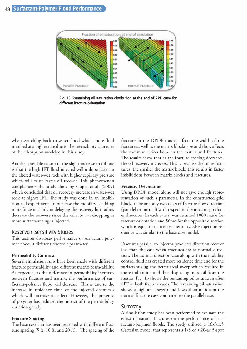
Surfactant-Polymer Flood Performance48
when switching back to water fl ood which more fl uid imbibed at a higher rate due to the reversibility character of the adsorption modeled in this study.
Another possible reason of the slight increase in oil rate is that the high IFT fl uid injected will imbibe faster in the altered water-wet rock with higher capillary pressure which will cause faster oil recover. Th is phenomenon complements the study done by Gupta et al. (2009) which concluded that oil recovery increase in water-wet rock at higher IFT. Th e study was done in an imbibi-tion cell experiment. In our case the mobility is adding more force not only in delaying the recovery but rather, decrease the recovery since the oil rate was dropping as more surfactant slug is injected.
Reservoir Sensitivity Studies Th is section discusses performance of surfactant poly-mer fl ood at diff erent reservoir parameter.
Permeability Contrast Several simulation runs have been made with diff erent fracture permeability and diff erent matrix permeability. As expected, as the diff erence in permeability increases between fracture and matrix, the performance of sur-factant-polymer fl ood will decrease. Th is is due to the increase in residence time of the injected chemicals which will increase its eff ect. However, the presence of polymer has reduced the impact of the permeability variation greatly.
Fracture Spacing Th e base case run has been repeated with diff erent frac-ture spacing (5 ft, 10 ft, and 20 ft). Th e spacing of the
fracture in the DPDP model aff ects the width of the fracture as well as the matrix blocks size and thus, aff ects the communication between the matrix and fractures. Th e results show that as the fracture spacing decreases, the oil recovery increases. Th is is because the more frac-tures, the smaller the matrix block; this results in faster imbibitions between matrix blocks and fractures.
Fracture Orientation Using DPDP model alone will not give enough repre-sentation of such a parameter. In the constructed grid block, there are only two cases of fracture fl ow direction (parallel or normal) with respect to the injector produc-er direction. In each case it was assumed 1000 made for fracture orientation and 50md for the opposite direction which is equal to matrix permeability. SPF injection se-quence was similar to the base case model.
Fractures parallel to injector producer direction recover less than the case when fractures are at normal direc-tion. Th e normal direction case along with the mobility control fl uid has created more residence time and for the surfactant slug and better areal sweep which resulted in more imbibition and thus displacing more oil from the matrix. Fig. 13 shows the remaining oil saturation after SPF in both fracture cases. Th e remaining oil saturation shows a high areal sweep and low oil saturation in the normal fracture case compared to the parallel case.
Summary A simulation study has been performed to evaluate the eff ect of natural fractures on the performance of sur-factant-polymer fl oods. Th e study utilized a 16x31x5 Cartesian model that represents a 1/8 of a 20-ac 5-spot
Fig. 13. Remaining oil saturation distibution at the end of SPF case for different fracture orientation.

Surfactant-Polymer Flood Performance
www.saudiarabiaoilandgas.com | SA O&G Issue 21
49
pattern unit. Fractures were incorporated in the CMG STARS with a dual-porosity dual-permeability model. Simulation runs were made in which the following pa-rameters were modifi ed: injection scenarios, matrix wet-tability, IFT, and fracture and matrix properties.
Conclusions Th e following main conclusions may be drawn from re-sults of the simulation study and results of studies by researchers as gleaned from literature:
• Defi ning contribution of spontaneous imbibitions on the total recovery is an important parameter for a suc-cessful chemical EOR pilot.
• When spontaneous imbibition contribution to recov-ery is high in the reservoir, low IFT surfactant polymer should be injected after optimum water saturation has been reached by water fl ooding in order to utilize the capillary force and maximize oil recovery.
• Water saturation in a mixed-wet fractured reservoir has high impact on the success of SPF.
• Only in oil-wet reservoir with no positive capillary pressure, injecting enhanced brine at initial water satu-ration will result in higher oil recovery than if injected at higher water saturation. A pre-fl ush injection has other benefi ts such as reducing salinity or ion exchange – this should be considered as to its eff ect on whether a pre-water injection will yield faster oil recovery or not.
• In the study of continuous injection or surfactant-pol-ymer fl ood, the result shows that in wettability altering surfactant, an optimum IFT should be combined in the surfactant eff ect. A change in the IFT eff ect from the optimum value will result in lower oil recovery.
• Th e smaller the permeability contrast between frac-tures and matrix, the higher the oil recovery. However, improved mobility will reduce this eff ect.
• When blockage is formed in the matrix blocks due to high chemical adsorption on the matrix, the injected fl uid channels through the fractures, giving an increase in water cut without decreasing the total liquid rate.
• Injecting water after surfactant-polymer slug injection will enhance the imbibition of water from the fractures into the matrix and remove some of the precipitate be-cause the matrix has been made more water-wet. Th ese results need further evaluation which was outside the scope of this study.
• Th e higher the fracture density, the higher the imbibi-tion rate which leads to a higher oil recovery. • Performance of surfactant polymer fl ood can be aff ect-ed positively or negatively by fracture orientation with respect to the injector-producer direction. Th e design of such EOR process should take into consideration this fracture parameter.
Recommendations Based on results obtained in this study, the following recommendations for research are made.
1. A validation of a fi eld scale simulation is required. Imbibition cell experiments may not adequately repre-sent fi eld conditions due to the lack of representation of viscous force. Research using a scaled quarter of 5-spot physical model containing a fractured porous medium is recommended.
2. Using the physical model mentioned in item 1 above, experimental research should be conducted to investi-gate the eff ect of injecting high IFT brine after wettabil-ity altering surfactant into the model.
Acknowledgments Most of this work is based on the research conducted to fulfi ll the requirements for an MS degree in Petroleum Engineering by Nawaf I. SayedAkram at Texas A&M University. I would like to thank Dr. D. Schechter, Texas A&M for his valued opinions through this work. I would like also to thank Saudi Aramco for the full scholarship on my master’s degree and granting the permission to publish this paper.
References Aldejain, A. A. 1999. Implementation of a Dual Poros-ity Model in a Chemical Flooding Simulator, PhD dis-sertation, Th e University of Texas, Austin, Texas.
Chen, J., Miller, M.A. and Sepehrnoori, K. 1995. In-vestigations of Matrix-Fracture Transfer Flows in Dual Porosity Modeling of Naturally Fractured Reservoirs. Paper SPE 29562 presented at the Rocky Mountain Re-gional/ low-Permeability Reservoirs Symposium, Den-ver, Colorado, 20-22 March.
Delshad, M., Najafabadi, N. F., Anderson, G., Pope, G. A. and Sepehrnoori, K. 2009. Modeling Wettability Alteration By Surfactants in Naturally Fractured Res-ervoirs. SPE Reservoir Evaluation & Engineering 12 (3): 361-370.
Delshad, M., Najafabadi, N. F. and Sepehrnoori, K.
Surfactant-Polymer Flood Performance50
2009. Scale Up Methodology for Wettability Modifi ca-tion in Fractured Carbonates. Paper SPE 118915-MS presented at the SPE Reservoir Simulation Symposium, Th e Woodlands, Texas, 2-4 February.
Gupta, R., Mohan, K. and Mohanty, K. K. 2009. Sur-factant Screening for Wettability Alteration in Oil-Wet Fractured Carbonates. Paper SPE presented at the SPE Annual Technical Conference and Exhibition, New Or-leans, Louisiana, 4-7 October.
Guzman, R. E. and Aziz, K. 1992. Fine Grid Simulation of Two-Phase Flow in Fractured Porous Media. Paper SPE 24916-MS presented at the SPE Annual Techni-cal Conference and Exhibition, Washington, D.C., 4-7 October.
Hirasaki, G. and Zhang, D. L. 2004. Surface Chemistry of Oil Recovery From Fractured, Oil-Wet, Carbonate Formations. SPE Journal 9 (2): 151-162.
Mohan, K. 2009. Alkaline Surfactant Flooding for Tight Carbonate Reservoirs. Paper SPE 129516-STU-P pre-sented at the SPE Annual Technical Conference and Ex-hibition, New Orleans, Louisiana, USA, 4-7 October.
Najafabadi, N. F., Delshad, M., Sepehrnoori, K., Nguy-en, Q. P. and Zhang, J. 2008. Chemical Flooding of Fractured Carbonates Using Wettability Modifi ers. Pa-per SPE 113369-MS presented at the SPE/DOE Sym-posium on Improved Oil Recovery, Tulsa, Oklahoma, 19-23 April.
Saad, N. and Sepehrnoori, K. 1989. Simulation of Big Muddy Surfactant Pilot. SPE Reservoir Engineering 4 (1): 24-34.
Schechter, D. S., Zhou, D. and Jr., F. M. O. 1991. Cap-illary Imbibition and Gravity Segregation in Low IFT Systems. Paper SPE 22594-MS presented at the SPE Annual Technical Conference and Exhibition, Dallas, Texas, 6-9 October.
Stegemeier, G. L. 1974. Relationship of Trapped Oil Saturation to Petrophysical Properties of Porous Media. Paper SPE 4754-MS presented at the SPE Improved Oil Recovery Symposium, Tulsa, Oklahoma, 22-24 April.
Taber, J. J. 1969. Dynamic and Static Forces Required To Remove a Discontinuous Oil Phase from Porous Me-dia Containing Both Oil and Water. Soc. Pet. Eng. J. 9 (1): 3 - 12.
Tarahhom, F., Sepehrnoori, K. and Marcondes, F. 2009. A Novel Approach to Integrate Dual Porosity Model and Full Permeability Tensor Representation in Frac-tures. Paper SPE 119001-MS presented at the SPE Res-ervoir Simulation Symposium, Th e Woodlands, Texas, 2-4 April.
Warren, J. E. and Root, P. J. 1963. Th e Behavior of Nat-urally Fractured Reservoirs. Soc. Pet. Eng. J. 3 (3): 245 - 255.


A Novel 4-D Reservoir Simulation Workfl ow for Optimizing Infl ow Control Device Designs in a Giant Carbonate Reservoir
By Oloruntoba Ogunsanwo, SPE, Schlumberger, Byung Lee, Hidayat Wahyu, SPE, Saudi ARAMCO, Edmund Leung, Varma Gottumukkala, Feng Ruan, SPE, Schlumberger Copyright 2011, Society of Petroleum Engineers This paper was prepared for presentation at the 2011 SPE Saudi Arabia Section Technical Symposium and Exhibition held in AlKhobar, Saudi Arabia, 15–18 May 2011. This paper was selected for presentation by an SPE program committee following review of information contained in an abstract submit-ted by the author(s). Contents of the paper have not been reviewed by the Society of Petroleum Engineers and are subject to correction by the author(s). The material, as presented, does not necessarily reflect any position of the Society of Petroleum Engineers, its officers, or members. Papers presented at the SPE meetings are subject to publication review by Editorial Committee of Society of Petroleum Engineers. Electronic reproduction, distribution, or storage of any part of this paper without the written consent of the Society of Petroleum Engineers is prohibited. Permission to reproduce in print is restricted to an abstract of not more than 300 words; illustrations may not be copied. The abstract must contain conspicuous acknowledgment of where and whom the paper was presented. Write Liberian, SPE, P.O. Box 833836, Richardson, TX 75083-3836, U.S.A., fax 01-972-952-9435.
Abstract A new 4-D infl ow control device optimisation work-fl ow has been developed using a sector model on the west fl ank of Field A, off shore Saudi Arabia. Th e ap-proach involves the application of time-lapse moni-toring of reservoir saturation profi les for injectors and producers as well as 4-D water fl ood front movement in the reservoir to understand dynamic reservoir chal-lenges. Th ese are zones of future water breakthrough, dynamic injection/production interaction, impact of reservoir drive mechanism on well injectivity or pro-ductivity, initial and future reservoir conditions.
With this understanding, an initial rate optimization process is performed with open hole injectors and producers. Th ereafter, the completion is optimized to achieve uniform infl ux profi le, fl ow control and zonal isolation where required along the horizontal section. Four diff erent completion strategies were evaluated
by alternating between Infl ow Control Device (Noz-zle based) completion and open hole in injectors and producers.
Th e sector model used in this study is subject to fur-ther calibrations as more geological, petrophysical and production data become available; the study outcome based on the novel workfl ow demonstrated the chal-lenges involved in determining a completion strategy with ICDs in injectors and producers. Th e results illus-trated an incremental cumulative oil gain of 5% with a one year delay in water breakthrough for a 20 year prediction. Moreover, further improvement in recov-ery can be attained with ICD completions above that achieved with rate optimization process alone.
Th e study demonstrates the positive impact that ICD completions can be benefi cial in challenging reservoirs with mobility ratios considerably greater than one.
4-D Reservoir Simulation Workflow52

Th e industry should consider this novel 4-D well – reservoir integrated modeling approach to assist in determining a completion strategy in evaluating ICD completion designs prior to deploying them in a fi eld wide campaign.
1. Introduction In order to achieve maximum reservoir contact in a carbonate fi eld with large hydrocarbon deposits, long horizontal wells are necessary to improve the produc-tivity and injectivity of producers and injectors re-spectively. However, the presence of a tight layer of tar deposit with very high viscosity underlying the produc-ing reservoir layers has prevented communication with the bottom water aquifer. In addition to heterogenei-ties in reservoir rock properties (permeability, poros-ity etc.), the viscosity of the oil also varies with depth. Th erefore, pattern or peripheral waterfl ood injection is necessary for pressure maintenance while producing from this fi eld. Even if reservoir rock properties were to be homogenous, challenges such as heel-to-toe eff ect will still be encountered for these long horizontal pro-duction/injection wells of 3000 – 6500 ft Open Hole (OH) sections. Th e eff ect will cause more production from the heel section and will usually lead to early wa-ter or gas breakthrough. In view of these challenges, the questions that need to be accounted for during the planning stage of water fl ooding scheme are summa-rised below.
• Will there be a relatively uniform injection profi le if Open Hole (OH) completions are adopted for the horizontal injectors ? • Will few reservoir zones dominate production in the OH horizontal producers ? • Will effi cient reservoir sweep be attained with a mini-mum number of injectors and producers ? • How can water channeling from injectors through high perm streaks be retarded by delaying water break-
through or minimizing water cut in producers ? • Can ICD completion strategy be adopted and if YES, how much more improvement in the fi eld recovery will it off er over OH completions ?
2. Principle and design of Infl owControl Devices (ICD) Th ere are various types of Infl ow Control Device (ICD); however, only the design and principle of nozzle based confi gurations will be discussed in this paper. Interested readers can refer to (Alkhelaiwi et al, 2007; Ellis et al, 2009; Ouyang 2009) for other types of ICD. A typical nozzle based ICD joint is a piece of blank pipe having wire wrapped sand screen for sand control or debris barrier for carbonate for-mation mounted on one end and fi tted with an ICD housing which protects the ceramic nozzles on the other end, Fig. 1. Th is section also utilises centralizers. Th ere are four to six nozzle ports in each of the ICD joints depending on application. Th e nozzle are in vari-ous sizes and are usually fi tted on the rig, based on a fi nal ICD tally design considering actual LWD well log data, other well and reservoir data. Each ICD joint is about 12m or 40 ft in length. Th e unique manufacturing process employed for the wire wrapped screen ensures a shrink fi t between the screen jacket and the base pipe. Th is provides the screen with the same mechanical strength as the base pipe and mak-ing it possible to rotate the ICD completion string while running in hole if required. With nozzle based ICDs, the design and optimization can be achieved by determining the number of ICDs, their nozzle sizes or confi gurations and packer placement. Th is fl exibility, provides a large number of possible nozzle size com-binations to achieve production control and optimi-zation in horizontal wells. Th is is a clear distinction between nozzle based devices compared to helical/tube ICD systems which do not off er this fl ex-ibility.
Figure 1: Typical Nozzle Based ICD with wire wrapped screen
4-D Reservoir Simulation Workflow
www.saudiarabiaoilandgas.com | SA O&G Issue 21
53

ICDs are designed to optimize production from hori-zontal completions by equalizing the reservoir infl ow along the entire length of the well bore. As shown in Fig.1, fl uid fl ow from the reservoir fl ows across the screen into the annulus between the screen and the base pipe and then fl ows through the nozzle into the inside of the base pipe. Th e fl uid fl ow from the reservoir into wellbore annulus is governed by Darcy Eq 1 while fl uid fl ow across the nozzles into inside of the base pipe is based on Bernoulli Eq 2 of an incompressible fl uid.
(1)
Where ΔPF = Drawdown pressure = PReservoir - P well fl ow (annulus) μ = fl uid viscosity k = Absolute permeability L = Length of reservoir section A = Cross-sectional area q = Volumetric fl owrate of the fl owing liquid cF = �L/ kA = 1/PI (PI: Productivity Index)
When fl uid fl ow across the nozzle, the potential energy
is transformed into kinetic energy and thus a control-led pressure drop between wellbore annulus and inside of the base pipe is generated to achieve the desired uniform infl ow profi le along the wellbore, equation 2. Th e pressure drop is proportional to square of the rate (velocity) and density, but independent of viscosity. Whereas, helical and tube ICD types which are both dependent on rate and fl uid viscosity can possibly pro-vide more or less pressure drop than required or initial-ly designed since fl uid properties change with increase in well water cut.
(2)
Where ΔPN = pressure drop in nozzles per joint (psi) ρ = fl uid density at reservoir conditions (ib/ft3) Q = volumetric rate of the fl owing fl uid per joint, [bbls/d] @ reservoir conditions A = infl ow area of nozzles per joint, [ft2] v = the fl uid velocity (ft/s) Cu = unit conversion constant Cv = the fl ow coeffi cient
Figure 2: Map view of the Field A Reservoir show-ing the sector model
Figure 3: Vertical cross section showing upper and lower reservoir units separated by tight low perm zone
4-D Reservoir Simulation Workflow54

Potential benefi ts of ICDs are not limited to:
• Correct heel to toe eff ect in long horizontal wellbore as accelerated produces from the heel section in a con-ventional completion (perforated liner). • Achieve uniform reservoir sweep and improve re-covery • Delay water or gas breakthrough and reduce well wa-ter cut in reservoirs with higher water mobility than oil and wellbore proximity to fl uid contacts • Prevent crossfl ow during production • Improve wellbore clean-up since fl uid is drained uni-formly along the wellbore. • Off er sand or debris control
3. Field Overview Th e fi eld comprises of carbonate reservoirs modeled as single porosity and permeability with no fracture net-work. It is located in the shallow waters of the Western Arabian Gulf, Saudi Arabia. Th e sector model used is a subset of Field A, Fig. 2. It has a down-dip structure towards the south. Two good reservoir zones are ob-served from south to north separated by a very very low permeability layer, Fig. 3. In the upper reservoir zone, there is a continuous and relatively high permeability zone at the bottom. However, in the lower reservoir zone, the relatively high permeability zone is located at the top of the section. A bottom water aquifer is interpreted to be connected to the reservoir from the south. However, the presence of a very high viscous Tarmat zone, (20–40 ft thickness and viscosity ranges above 3000 cP) underneath the oil column disconnects the aquifer from the reservoir; thus, leaving the reser-voir to a depletion drive mechanism. Consequently, for effi cient fi eld recovery, a peripheral water injection scheme has been considered prior to starting the next
phase of fi eld production to improve reservoir sweep and pressure maintenance. Th e reservoir fracture gradi-ent is 0.75 psi per foot TVD. Diff erent fl ow units with diff erent saturation regions from the special core analy-sis data have been identifi ed in the two zones. Th ey extend from north to south.
It is an undersaturated reservoir with crude oil gravity of 26 0API. Th e initial reservoir pressure is an order of magnitude greater than bubble point. Th e oil column and water viscosities at initial reservoir conditions are 4.22 cP and 0.4 cP respectively. Water in the reservoir has a much higher mobility than oil. Mobility ratio at water breakthrough is considerably greater than one. Th erefore, water channeling through the oil will be a major challenge for the water fl ooding scheme.
4. Challenges Th e reservoir challenges observed in Field A have been categorized below based on reservoir heterogeneities and structural complexities.
• Rapid reservoir pressure decline due to the presence of a tarmat zone preventing the producing reservoir layers from
communicating with the bottom aquifer water • Reservoir uncertainty associated with the areal distri-bution of the Tarmat zone across the Field - Reservoir characterization - Th e placement of some of the injectors inside the Tarmat zone
• Areal and vertical variation of the permeability pro-fi le distribution across the fi eld, Fig. 3. Th ere are high permeability streaks at the bottom section of the up-per reservoir zone. Th is is aided by gravity segregation,
Figure 4: 3-D mobility ratio distribution and Histogram for the Oil Column zone above the Tarmat
4-D Reservoir Simulation Workflow
www.saudiarabiaoilandgas.com | SA O&G Issue 21
55

which will lead to early water breakthrough in the pro-ducers. Th e reservoir heterogeneity will yield uneven water injection and oil production profi le; thereby, re-ducing oil recovery. • When the mobility ratio is greater than one at water breakthrough considering that oil viscosity is an order of magnitude higher than water viscosity, Fig. 4. Th is is further magnifi ed as diff erent fl ow units with diff erent saturation regions have been identifi ed. • Long Open Hole section for the producers and injec-tors, about 3000 and 6000 ftMD respectively. • Establishing optimum injection and production rates. • Completion selection and optimization.
5. Objectives and Scope Owing to the highlighted reservoir challenges, the study has been conducted to understand the optimum completion strategy for the injectors and producers that will improve recovery and reservoir sweep, delay water breakthrough and decrease water cut. A novel workfl ow process was developed and used to study the project objectives below.
• With the aid of 4-D dynamic modeling, identify fac-tors that signifi cantly impacts recovery. • Establish optimum injection and production rates • Perform various sensitivities on ICD completion de-sign • Determine optimum completion strategy that will improve recovery. Evaluate the diff erent nozzle based ICD completion strategy and compare each with the open hole base case. - ICD in Injector and ICD in Producer - ICD in Injector and Open Hole (OH) in Producer - OH in Injector and ICD in Producer - Base case: OH in Injector and OH in Producer
Th e study is based on a sector model of Field A in Sau-di Arabia. Th ere are six horizontal producers and three horizontal injectors. Th e injectors are aligned in the fi rst row, followed by second and third rows of the pro-ducers. Th is geological model was built in seismic to simulation software, PetrelTM. Th e rate optimization process was simulated using Patterned Flooding Man-agement Optimizer, PFM, using a streamline simula-tor, FrontSimTM. Multisegment well option and ad-vanced ICD completion were modeled and simulated using a grid based numerical simulator, ECLIPSETM. Using Pattern Flood Management (PFM) optimizer in FrontSim, optimum injection rates for the periph-eral water fl ooding scheme and production rates will be assessed. Th ese optimized rates will be the basis for
evaluating the potential benefi ts of an optimized noz-zle based ICD completion design over standard open hole wells.
6. Workfl ow Background 6.1 Traditional well centric Workfl ow In traditional wellbore centric approach, the optimum completion design is achieved by distributing ICDs based on near wellbore permeability profi le and per-forming sensitivities on number of ICDs, ICD nozzle sizes, number of packers and its placement. Th e main objective is to achieve infl ux balancing along the hori-zontal open hole (OH) section, minimize or eliminate heel-to-toe eff ect and reduce well water cut. Th e opti-mum ICD completion design will be selected based on incremental fi eld cumulative oil gain over OH hori-zontal wells and a minimum pressure drop across the ICD completion.
However, in reservoirs with mobility ratios considerably greater than one, gravity drainage dominated and hav-ing a water injection scheme, stimulating relatively low permeable zones with ICDs can be a source of future water entry leading to high water cut in producers and ultimately lower oil recovery than conventional com-pletions. Th is methodology may even lead to a wrong completion strategy if adopted in fi eld wide reservoir studies with wells intended for ICD completions.
6.2 Novel 4-D well – reservoir integrated dynamic modeling workfl ow Th e approach that will be discussed in this novel 4-D well – reservoir integrated workfl ow, Fig. 5, is that distributing ICDs using wellbore permeability as per-formed in traditional well centric approach is insuffi -cient because it fails to consider the eff ects of reservoir heterogeneities and dynamics on well performance as listed below. Moreover, these factors change with time as well as their impact on well performance.
• Eff ects of reservoir connectivity and interference with neighboring wells to account for future water breakthrough • Water fl ood front movement in the reservoir • Injection/production interaction dynamics Completion selection and optimization. • Th e impact of reservoir drive mechanism on well productivity or injectivity • Initial and future reservoir conditions.
Th is approach is based on performing 4-D dynamic modeling using a history matched reservoir model. Th ereafter, using Time-Lapse signature (4-D) of PLT/
4-D Reservoir Simulation Workflow56

FSI and reservoir saturation profi le near the wellbore for injectors and producers and 4-D water fl ood front monitoring, the reservoir engineer will understand how these reservoir drivers change over time. With this insight, one can then re-distribute ICD completions along the horizontal section to achieve either infl ux balancing, control or zonal isolation as required. One can decide whether a zone requires infl ux balancing or fl ow restriction at the beginning of well production or injection. For instance, if there will be early future wa-ter breakthrough or high water saturation from a zone due to the producer trajectory dipping downward in the reservoir layer and its interaction with neighboring injectors, such that the zone requires only fl ow restric-tion or isolation. Th erefore, the number of ICDs and nozzle size sensitivities will be designed to counter the negative impact of these reservoir drivers. Th e work-fl ow will be elucidated in the simulation results sec-tion.
7. Novel 4-D Well ReservoirIntegrated Workfl ow 7.1 Summary of Novel 4-D Well – ReservoirIntegrated Dynamic Modeling Workfl ow Th e individual steps for designing ICD completion in the novel 4-D workfl ow, Fig. 5, are outlined below.
1. Th e workfl ow starts by creating a sector model from full fi eld model (FFM) that has been history matched.
2. Rates optimization process for the open hole injec-tors and producers was performed using a PFM opti-mizer in a streamline simulator to determine optimum injection and production rates.
3. Since the geological model was built in Seismic to Simulation modelling application, the completion strategy for the horizontal injectors and producers were designed by populating ICD completion (Nozzle based ICD joint, add-on / slip-on packers, reamer shoe at end of completion string) along the wellbore. Th e ICD design methodology that is being proposed in this paper will be further elucidated in the detail section.
4. An advanced multi-segment well model was incor-porated into ICD completion for the injectors and producers using a homogenous fl ow model, which considers all phases fl owing with the same velocity.
5. Th e results of the rate optimization sensitivities from the PFM optimizer was inputted into the development strategy of the simulation cases considered in the grid based numerical simulator. Th is simulator was select-ed because of its capability to simulate injection and production performance of horizontal wells with ICD completions.
6. Various cases using diff erent ICD completion de-signs and sensitivities were defi ned and simulated.
Figure 5: Novel 4-D well-reservoir integrated dynamic workflow
4-D Reservoir Simulation Workflow
www.saudiarabiaoilandgas.com | SA O&G Issue 21
57
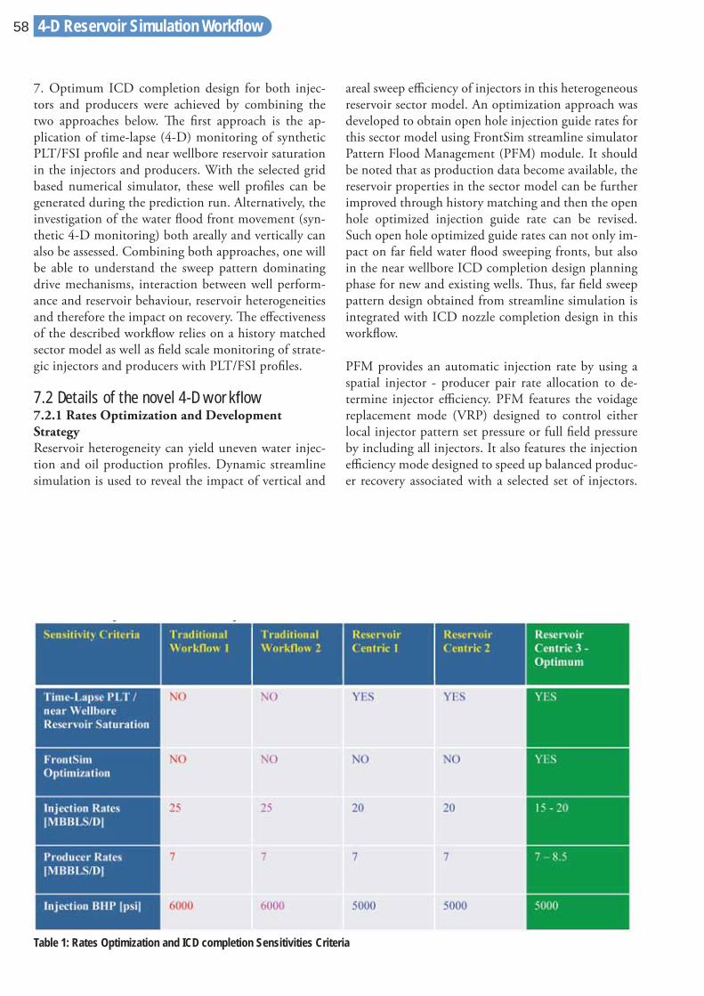
7. Optimum ICD completion design for both injec-tors and producers were achieved by combining the two approaches below. Th e fi rst approach is the ap-plication of time-lapse (4-D) monitoring of synthetic PLT/FSI profi le and near wellbore reservoir saturation in the injectors and producers. With the selected grid based numerical simulator, these well profi les can be generated during the prediction run. Alternatively, the investigation of the water fl ood front movement (syn-thetic 4-D monitoring) both areally and vertically can also be assessed. Combining both approaches, one will be able to understand the sweep pattern dominating drive mechanisms, interaction between well perform-ance and reservoir behaviour, reservoir heterogeneities and therefore the impact on recovery. Th e eff ectiveness of the described workfl ow relies on a history matched sector model as well as fi eld scale monitoring of strate-gic injectors and producers with PLT/FSI profi les.
7.2 Details of the novel 4-D workfl ow 7.2.1 Rates Optimization and DevelopmentStrategy Reservoir heterogeneity can yield uneven water injec-tion and oil production profi les. Dynamic streamline simulation is used to reveal the impact of vertical and
areal sweep effi ciency of injectors in this heterogeneous reservoir sector model. An optimization approach was developed to obtain open hole injection guide rates for this sector model using FrontSim streamline simulator Pattern Flood Management (PFM) module. It should be noted that as production data become available, the reservoir properties in the sector model can be further improved through history matching and then the open hole optimized injection guide rate can be revised. Such open hole optimized guide rates can not only im-pact on far fi eld water fl ood sweeping fronts, but also in the near wellbore ICD completion design planning phase for new and existing wells. Th us, far fi eld sweep pattern design obtained from streamline simulation is integrated with ICD nozzle completion design in this workfl ow.
PFM provides an automatic injection rate by using a spatial injector - producer pair rate allocation to de-termine injector effi ciency. PFM features the voidage replacement mode (VRP) designed to control either local injector pattern set pressure or full fi eld pressure by including all injectors. It also features the injection effi ciency mode designed to speed up balanced produc-er recovery associated with a selected set of injectors.
Table 1: Rates Optimization and ICD completion Sensitivities Criteria
4-D Reservoir Simulation Workflow58

Th e VRP control option of PFM was used to set up multiple scenario runs using the Petrel optimizer with an aim to understand sensitivities of injector and pro-ducer operating constraints. Th e results were fed into the development strategy of the grid based numerical simulator. In order to use the optimized development strategy plan from the optimizer for ICD design in the grid based numerical simulator, the same simulation case was run in ECLIPSE and the production and pres-sure responses were compared. Th e results from both simulators agreed.
7.2.2 Completion strategy, well segmentation and development strategy In the completion strategy, one is expected to distribute along the OH section of the injectors and producers using various ICD design sensitivities. Th e completion design is performed by considering in isolation, the concept of traditional and 4-D workfl ow methodolo-gies. Each ICD design was simulated considering the completion strategy stated in the project study objec-tives.
Th e injectors and producers were modeled using mul-ti-segment well modeling, MSW, by dividing the well-bore into a series of 1 – dimensional segments. Th is will enable accurate modeling of multiphase fl ow in the wellbore, eff ects of multilateral topology of the well path on the fl uid behavior, complex crossfl ow ef-fects, and fl ow across ICDs. Homogeneous fl ow model where all the phases fl ow with the same velocity was adopted with the MSW option (ECLIPSE technical Manual 2010).
For the purpose of comparing results from both work-fl ows, some ICD design sensitivities were performed based on traditional workfl ow concept while others were conducted on the basis of the 4-D workfl ow. Th is paper presents the fi nal two and three sensitivities of traditional and 4-D well– reservoir integrated work-fl ows respectively by comparing OH/OH vs. ICD/ICD completion strategy for both injectors and producers, Table 1. Other disparities in the development strategy are in injection rates, injection BHP constraints and the use of rate optimization process results.
Sensitivity criteria considered in addition to Table 1 were
• Number of ICDs in injectors and producers • ICD nozzle size • Number of packers • Packer spacing
8. Summary of Simulation Results Th is section discusses the simulation results of the project study based on six horizontal producers and three horizontal injectors. Th e simulation runs were conducted for a 20 year period. Th e results emphasize the benefi ts of using the new approach to identifying optimized ICD design. Th ey also promote a departure from the traditional method of using only permeability profi le to identify optimum design because this can of-ten lead to poor ICD design and completion strategy. It demonstrates the importance of considering other dy-namic reservoir responses through 4-D dynamic mod-eling to understand their eff ects on well performance and thereafter ICD design to counter or promote the behavior. Th is study has proposed a novel workfl ow to designing an optimum ICD completion design. How-ever, the results obtained from traditional workfl ow are compared against the optimum ICD completion de-sign to further illustrate the new 4-D workfl ow.
Th e simulation cases ran for each set of development strategy, considers the scenarios below; however, only the ICD completion strategy 3 will be reported.
• Base Case: OH Injectors and OH producers • ICD Strategy 1: ICD Producers and OH Injectors • ICD Strategy 2: OH Producers and ICD Injectors • ICD Strategy 3: ICD Producers and ICD Injectors
8.1 Criteria for Optimum ICD Completion Design Th e Optimum ICD design can be selected by compar-ing additional recovery and fi eld wide fl owing bottom hole pressure of various ICD design sensitivities per-formed for each ICD completion strategy against an OH Case. Th e criteria are but not limited to:
• Extent of incremental fi eld cumulative oil produc-tion of ICD strategy over the OH case. • Compare fi eld pressure of the three optimum ICD Completion strategies against the OH base case. • Compare fi eld pressure of various sensitivities for each ICD completion strategy separately against the OH base case. • Reduction in well/fi eld water cut for ICD over OH case. • Delay in water breakthrough time between an ICD and OH case. • Qualitatively assess reservoir sweep of individual ICD strategy on well basis over OH.
8.2 Results of PFM and ICD Design Sensitivities Th e initial optimization results reveal that a simple increase of injection rates can lead to a reduction of
4-D Reservoir Simulation Workflow
www.saudiarabiaoilandgas.com | SA O&G Issue 21
59
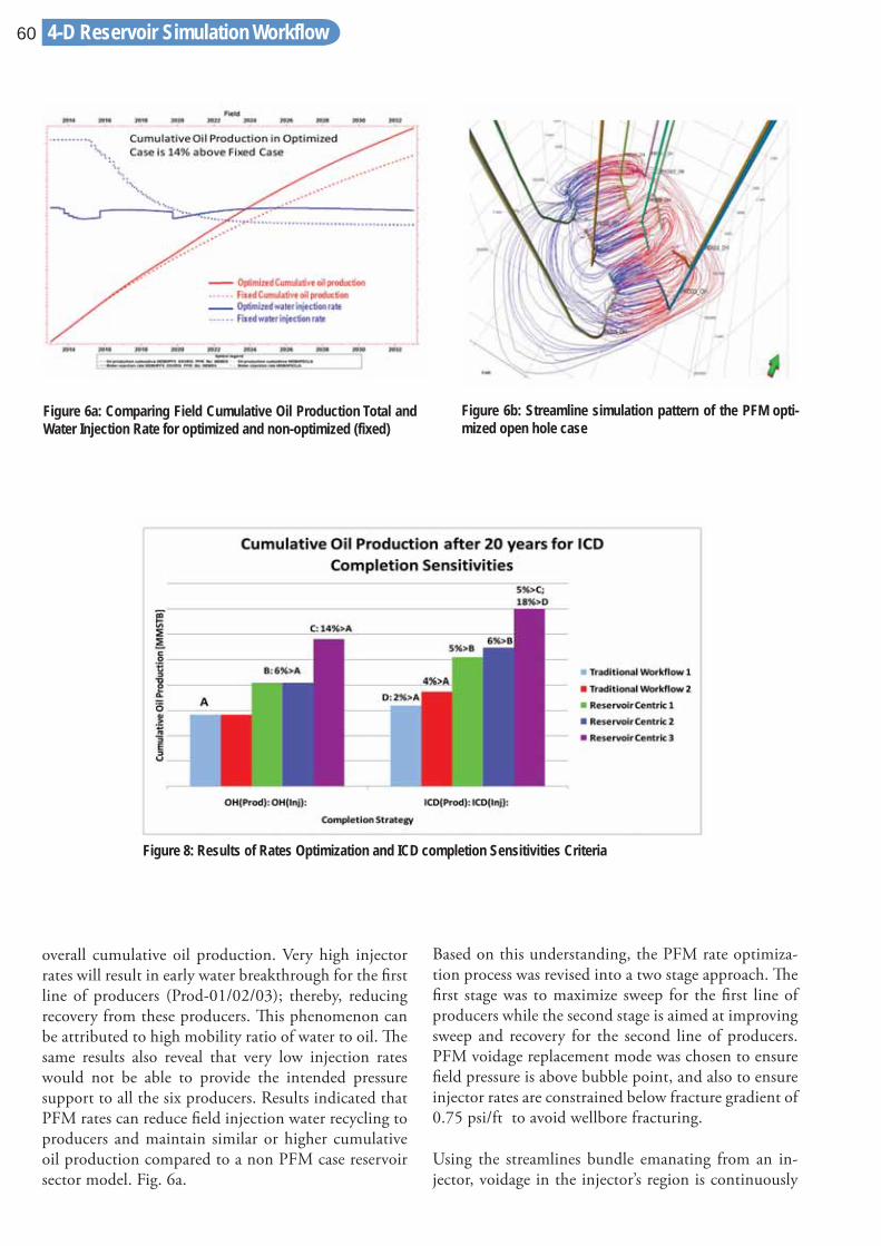
overall cumulative oil production. Very high injector rates will result in early water breakthrough for the fi rst line of producers (Prod-01/02/03); thereby, reducing recovery from these producers. Th is phenomenon can be attributed to high mobility ratio of water to oil. Th e same results also reveal that very low injection rates would not be able to provide the intended pressure support to all the six producers. Results indicated that PFM rates can reduce fi eld injection water recycling to producers and maintain similar or higher cumulative oil production compared to a non PFM case reservoir sector model. Fig. 6a.
Based on this understanding, the PFM rate optimiza-tion process was revised into a two stage approach. Th e fi rst stage was to maximize sweep for the fi rst line of producers while the second stage is aimed at improving sweep and recovery for the second line of producers. PFM voidage replacement mode was chosen to ensure fi eld pressure is above bubble point, and also to ensure injector rates are constrained below fracture gradient of 0.75 psi/ft to avoid wellbore fracturing.
Using the streamlines bundle emanating from an in-jector, voidage in the injector’s region is continuously
Figure 6a: Comparing Field Cumulative Oil Production Total and Water Injection Rate for optimized and non-optimized (fixed)
Figure 6b: Streamline simulation pattern of the PFM opti-mized open hole case
Figure 8: Results of Rates Optimization and ICD completion Sensitivities Criteria
4-D Reservoir Simulation Workflow60
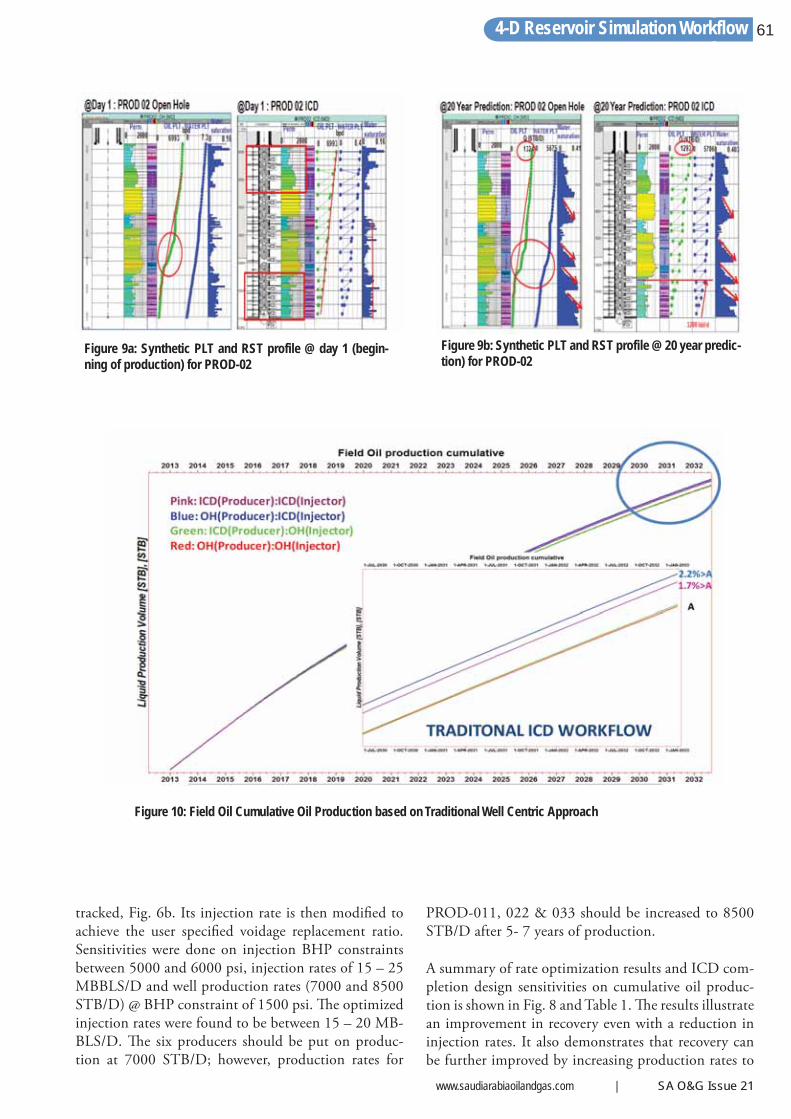
tracked, Fig. 6b. Its injection rate is then modifi ed to achieve the user specifi ed voidage replacement ratio. Sensitivities were done on injection BHP constraints between 5000 and 6000 psi, injection rates of 15 – 25 MBBLS/D and well production rates (7000 and 8500 STB/D) @ BHP constraint of 1500 psi. Th e optimized injection rates were found to be between 15 – 20 MB-BLS/D. Th e six producers should be put on produc-tion at 7000 STB/D; however, production rates for
PROD-011, 022 & 033 should be increased to 8500 STB/D after 5- 7 years of production.
A summary of rate optimization results and ICD com-pletion design sensitivities on cumulative oil produc-tion is shown in Fig. 8 and Table 1. Th e results illustrate an improvement in recovery even with a reduction in injection rates. It also demonstrates that recovery can be further improved by increasing production rates to
Figure 9a: Synthetic PLT and RST profile @ day 1 (begin-ning of production) for PROD-02
Figure 9b: Synthetic PLT and RST profile @ 20 year predic-tion) for PROD-02
Figure 10: Field Oil Cumulative Oil Production based on Traditional Well Centric Approach
4-D Reservoir Simulation Workflow
www.saudiarabiaoilandgas.com | SA O&G Issue 21
61

8500 STB/D after 5 -7 years for PROD-011, 022 and 033.
Th e rates optimization process further recommended injection and production rates that will achieve opti-mum fi eld cumulative oil production with minimum pressure loss across the ICDs. Th e results also illustrates that designing ICD completions based on traditional workfl ow concept will yield lower cumulative oil pro-duction than ICD completion based on the new 4-D well-reservoir integrated dynamic modeling workfl ow. Field recovery can be achieved by optimizing injector and producer rates alone but with the introduction of ICD completions, recovery can be further improved.
8.3 Traditional Well Centric Approach Results ICD design in traditional well centric approach is per-formed by increasing number of ICDs and/ or choos-ing a higher nozzle size, reducing packer spacing etc. in low permeability zone with reverse of these param-eters in high permeability zone along the horizontal section as shown by the rectangular boxes, Fig. 9a(@
day 1:Prod 02 ICD. Th is type of ICD design produces uniform cumulative oil PLT profi le at the start of pro-duction. However, on evaluating the PLT profi le and near wellbore reservoir saturation of the producers us-ing Time-Lapse technique, it will be observed that this approach failed to consider factors aff ecting fl uid fl ow behavior and their impacts on well production per-formance as explained in the 4-D workfl ow above. Th e concept of Time-Lapse technique mentioned in this paper involves investigating well injection and produc-tion profi les at diff erent future time steps where factors aff ecting fl uid fl ow behavior away from the wellbore are expected to be fully acting. For instance, Fig. 9b, (@ 20 year prediction: Prod 02 ICD, the cumulative water PLT profi le showed that more than 50% of water production in this well (Prod-02) would be produced from the toe section in the future. Th is is simply be-cause fi ve ICD joints are placed in this 750 ft interval with each ICD joint in a sub-compartment of about 150 ft. Th is section is being over produced. As a re-sult, producers in completion strategy of ICD comple-tion in both injectors and producers were producing
Figure 11: Field Cumulative Oil Production based on novel 4-D integrated well – reservoir workflow
4-D Reservoir Simulation Workflow62

higher water cut than producers in completion strategy of ICD completion in Injectors and OH producers, Fig. 9b. Cumulative oil production obtained from ap-plying traditional well centric concepts showed ICD completion in Injectors and OH producers as the best completion strategy, Fig. 10. Th is is a fl awed approach because it does not consider the impact of reservoir dy-namics. Please note that only one well plot is displayed for illustration purpose but similar eff ects are seen in the other producers.
8.4 Results of Novel Well – Reservoir Integrated Dynamic Modeling Workfl ow Results Th e results of the well-reservoir integrated dynamic
modeling approach indicated the optimum completion strategy as ICD completion in injectors and producers, Fig. 11. Th e results were achieved by carefully using Time Lapse technique (4-D) for PLT profi les and res-ervoir saturation in addition to wellbore permeability profi le to understand future water entry zone i.e. heel to toe and the impact of gravity on sweep patterns and well performance, Fig. 12a. Th is explains why fewer numbers of ICDs have been placed in the low perme-ability section near the toe of the producers since this section will experience high water saturation in the fu-ture and will be the source of future water entry into the well if over produced with a high number of ICDs and/or larger nozzle sizes. Fig. 12b illustrates the injec-
Figure 12a: Synthetic PLT and RST profile @ 20 year pre-diction (Time-Lapse approach) for PROD-02 using 4-D inte-grated well-reservoir workflow.
Figure 12b: Synthetic PLT and RST profile @ 20 year predic-tion (Time-Lapse approach) for INJ-02 using 4-D integrated well-reservoir workflow.
Figure 13: Field Pressure and Production Rates for the six pro-ducers ICD / ICD vs. OH base case based on novel 4-D inte-grated well – reservoir workflow
Figure 14: Field Cumulative Water Injection for the three Injec-tors based on novel 4-D integrated well – reservoir workflow
4-D Reservoir Simulation Workflow
www.saudiarabiaoilandgas.com | SA O&G Issue 21
63
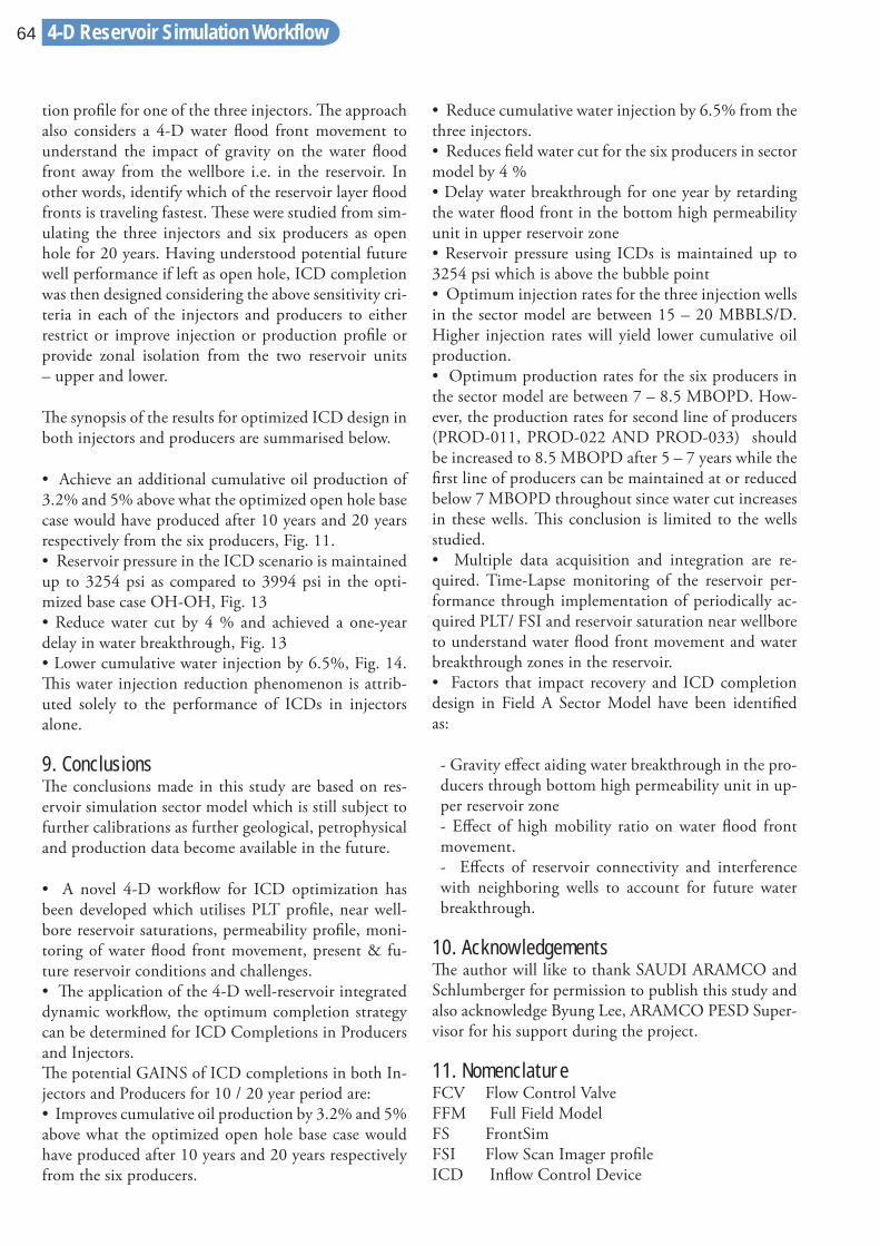
tion profi le for one of the three injectors. Th e approach also considers a 4-D water fl ood front movement to understand the impact of gravity on the water fl ood front away from the wellbore i.e. in the reservoir. In other words, identify which of the reservoir layer fl ood fronts is traveling fastest. Th ese were studied from sim-ulating the three injectors and six producers as open hole for 20 years. Having understood potential future well performance if left as open hole, ICD completion was then designed considering the above sensitivity cri-teria in each of the injectors and producers to either restrict or improve injection or production profi le or provide zonal isolation from the two reservoir units – upper and lower.
Th e synopsis of the results for optimized ICD design in both injectors and producers are summarised below.
• Achieve an additional cumulative oil production of 3.2% and 5% above what the optimized open hole base case would have produced after 10 years and 20 years respectively from the six producers, Fig. 11. • Reservoir pressure in the ICD scenario is maintained up to 3254 psi as compared to 3994 psi in the opti-mized base case OH-OH, Fig. 13 • Reduce water cut by 4 % and achieved a one-year delay in water breakthrough, Fig. 13 • Lower cumulative water injection by 6.5%, Fig. 14. Th is water injection reduction phenomenon is attrib-uted solely to the performance of ICDs in injectors alone.
9. Conclusions Th e conclusions made in this study are based on res-ervoir simulation sector model which is still subject to further calibrations as further geological, petrophysical and production data become available in the future.
• A novel 4-D workfl ow for ICD optimization has been developed which utilises PLT profi le, near well-bore reservoir saturations, permeability profi le, moni-toring of water fl ood front movement, present & fu-ture reservoir conditions and challenges. • Th e application of the 4-D well-reservoir integrated dynamic workfl ow, the optimum completion strategy can be determined for ICD Completions in Producers and Injectors. Th e potential GAINS of ICD completions in both In-jectors and Producers for 10 / 20 year period are: • Improves cumulative oil production by 3.2% and 5% above what the optimized open hole base case would have produced after 10 years and 20 years respectively from the six producers.
• Reduce cumulative water injection by 6.5% from the three injectors. • Reduces fi eld water cut for the six producers in sector model by 4 % • Delay water breakthrough for one year by retarding the water fl ood front in the bottom high permeability unit in upper reservoir zone • Reservoir pressure using ICDs is maintained up to 3254 psi which is above the bubble point • Optimum injection rates for the three injection wells in the sector model are between 15 – 20 MBBLS/D. Higher injection rates will yield lower cumulative oil production. • Optimum production rates for the six producers in the sector model are between 7 – 8.5 MBOPD. How-ever, the production rates for second line of producers (PROD-011, PROD-022 AND PROD-033) should be increased to 8.5 MBOPD after 5 – 7 years while the fi rst line of producers can be maintained at or reduced below 7 MBOPD throughout since water cut increases in these wells. Th is conclusion is limited to the wells studied. • Multiple data acquisition and integration are re-quired. Time-Lapse monitoring of the reservoir per-formance through implementation of periodically ac-quired PLT/ FSI and reservoir saturation near wellbore to understand water fl ood front movement and water breakthrough zones in the reservoir. • Factors that impact recovery and ICD completion design in Field A Sector Model have been identifi ed as:
- Gravity eff ect aiding water breakthrough in the pro-ducers through bottom high permeability unit in up-per reservoir zone - Eff ect of high mobility ratio on water fl ood front movement. - Eff ects of reservoir connectivity and interference with neighboring wells to account for future water breakthrough.
10. Acknowledgements Th e author will like to thank SAUDI ARAMCO and Schlumberger for permission to publish this study and also acknowledge Byung Lee, ARAMCO PESD Super-visor for his support during the project.
11. Nomenclature FCV Flow Control Valve FFM Full Field Model FS FrontSim FSI Flow Scan Imager profi le ICD Infl ow Control Device
4-D Reservoir Simulation Workflow64

LWD Logging while Drilling MSW ECLIPSE Multi-Segment Well Model OH Open Hole PESD Aramco Petroleum Engineering Support Division PFM FrontSim Patterned Flood Module Optimizer PLT Production Logging Tool Profi le PVT Pressure, Volume and Temperature PWI Power Water Injector RST Reservoir Saturation Profi le VRP Voidage Replacement Ratio Control mode
12. References 1. Dake, L. P., 1998: Fundamentals of Reservoir Engi-neering, Elsevier Science B.V., pp 337 - 367.
2. Ellis, T., Erkal A., Goh, G., Jokela T., Kvernstuen, S., Leung, E., Moen, T., Porturas, F., Skillingstad, T., Vorkinn, P.B., Raff n, A.G., “Infl ow Control Devices – Raising Profi les”, Oilfi eld Review Winter 2009/2010, p30-37.
3. Holmes, J. A., Barkve, T. and Lund, O., 1998. “Ap-plication of a Multi-segment Well Model to Simulate Flow in Advanced Wells.” SPE 50646, presented at the SPE European Petroleum Conference, Th e Hauge, Th e Netherlands, 20-22 October.
4. Leung, E., Nukhaev, M., Gottumukkala, M., Samo-sir, H., Abd El-Fattah, M., Ogunsanwo, O., Gonzalez, A., 2010 “Horizontal Well Placement and Completion Optimisation in Carbonate Reservoirs” SPE 140048, presented at the SPE Caspian Carbonates Technology Conference, Atyrau, Kazakhstan, November 2010.
5. Neylon, K. J., Reiso, E., Holmes, J. A. and Neese,
O. B. 2009. “Modeling Well Infl ow Control with Flow in Both Annulus and Tubing.” SPE 118909, present-ed at the SPE Reservoir Simulation Symposium, Th e Woodlands, Texas, USA, 2-4 February.
6. Ouyang, L.B., “Practical Consideration of Infl ow Control Device Application for Reducing Water Pro-duction”, SPE 124154, SPE Technical Conference and Exhibition, New Orleans, Louisiana, U.S.A., October 2009.
7. Raff n, A.G., Hundsnes S., Kvernstuen, S., Moen, T. 2007 “ICD Screen Technology Used To Optimize Wa-terfl ooding in Injector Well” SPE 106018, presented at the Production and Operations Symposium, Okla-homa, U.S.A., 31 March – 3 April.
8. Rahimah, A.K., Azrul, N.M., Goh, K.F., Asyikin, A.N., Leung, E., Johan, M. 2010. “Horizontal Well Optimization with Infl ow Control devices (ICDs) Ap-plication in Heterogeneous and Dipping Gas-Capped Oil Reservoirs” SPE 133336, presented at the SPE Annual Technical Conference and Exhibition held in Florence, Italy, 19-22 September.
9. Shahri, A., M., Kilany, K., Hembling, D., Lauritzen, J., E., Gottumukkala, V., Ogunyemi, O., Becerra, O.: 2009: Best “Cleanup Practices for an Off shore Sand-stone Reservoir with ICD completions in Horizontal wells” SPE 120651.
10. Schlumberger, 2010. FRONTSIM 2010.1 Techni-cal Description.
11. Schlumberger, 2010. ECLIPSE 2010.1 Technical Description.
4-D Reservoir Simulation Workflow
www.saudiarabiaoilandgas.com | SA O&G Issue 21
65

By Wael Abdallah, SPE, Weishu Zhao, SPE, and Ahmed Gmira, SPE, Schlumberger, Ardiansyah Negara, SPE, King Abdullah University of Science and Technology, and Jan Buiting, SPE, Saudi Aramco.
Copyright 2011, Society of Petroleum Engineers
This paper was prepared for presentation at the 2011 SPE Saudi Arabia Section Technical Symposium and Exhibition held in AlKhobar, Saudi Arabia, 15–18 May 2011.
This paper was selected for presentation by an SPE program committee following review of information contained in an abstract submit-ted by the author(s). Contents of the paper have not been reviewed by the Society of Petroleum Engineers and are subject to correction by the author(s). The material, as presented, does not necessarily reflect any position of the Society of Petroleum Engineers, its officers, or members. Papers presented at the SPE meetings are subject to publication review by Editorial Committee of Society of Petroleum Engineers. Electronic reproduction, distribution, or storage of any part of this paper without the written consent of the Society of Petroleum Engineers is prohibited. Permission to reproduce in print is restricted to an abstract of not more than 300 words; illustrations may not be copied. The abstract must contain conspicuous acknowledgment of where and whom the paper was presented. Write Liberian, SPE, P.O. Box 833836, Richardson, TX 75083-3836, U.S.A., fax 01-972-952-9435.
Sensitivity Analysis of Interfacial Tension on Saturation and Relative Permeability Model Predictions
Abstract Interfacial tension (IFT) measurements of Dodecane/brine systems at diff erent concentrations and Dodecane/deionized water subject to diff erent Dodecane purifi ca-tion cycles were taken over extended durations at room temperature and pressure to investigate the impact of aging. When a fresh droplet was formed, a sharp drop in IFT was observed assumed to be a result of intrinsic impurity adsorption at the interface. Th e subsequent measurements exhibited a prolonged equilibration pe-riod consistent with diff usion from the bulk phase to the interface. Our results indicate that minute amounts of impurities present in experimental chemical fl uids “used as received” have a drastic impact on the properties of the interface. Initial and equilibrium IFT are shown to be dramatically diff erent, therefore it is important to be cautious of utilizing IFT values in numerical mod-els. Th e study demonstrates the impact these variations in IFT have on relative permeability relationships by adopting a simple pore network model simulation.
Introduction Understanding the reservoir and what can be done to maximize oil recovery continues to be an active area of research; quite simply we typically only produce about 30-40% of original oil in place (OOIP) (Swenson et al., 2011; Shen et al., 2006). Th e fundamentals dominat-ing hydrocarbon recovery don’t change but the reservoir models used to evaluate such recovery scenarios can be improved by better understanding the fundamental in-teraction mechanism of fl uid/brine/rock systems and its chemistry. Core fl ooding and centrifugal methods are commonly used to determine recovery factor, relative permeability, capillary pressure, and the overall effi cien-cy of the fl ooding process. Th ese techniques are applied for all types of improved or enhanced oil recovery tech-niques – water, engineered or “Smart” water; chemical or miscible gas injection. Generally this is performed through preserved cores cut from the target formation or increasingly through numerically simulated cores mimicing the rock and reservoir conditions. As with all
Sensitivity Analysis of Interfacial Tension66

laboratory techniques, the value of the results depends entirely on how representative the acquired core plugs and fl uid samples are. Th e extended durations required to perform representative dynamic core fl oods , coupled with limited preserved core samples also, limit the range of fl ooding experiments that can be achieved. Numeri-cal techniques of course, (Koplik et. al., 1989; Venturoli and Boek, 2006; Kovscek et. al., 1993), allow one to simulate as many fl ooding scenarios as required. Clearly results are critically dependent on the quality of porous media representation, the fl uids and wetting status mod-eled therein. Before one accepts the outputs of a numeri-cal technique, one has to comprehend the impact of a wide range of parameters as demonstrated in Figure 1.
Two key parameters that have attracted interest in the past are the roles of interfacial tension between the two immiscible liquids and surface rock wettability. Th ese two parameters among others are key to mathemati-cally predicting relative permeability that can be fed into reservoir simulation models; most commonly used to compare and evaluate EOR methods prior to fi eld deployment. With fl uids interaction, a reduction in IFT decreases capillary pressure and increases capillary number, which increases the mobilization of trapped oil through the rock pore structure. Interaction with the rock pore structure, wettability describes how immisci-ble fl uids adhere to a rock surface infl uencing a variety of parameters pertaining to oil fl ow. Th e fl uid distri-bution in predominantly oil-wet rocks is signifi cantly diff erent to that in water-wet rocks. In the former, oil occupies more fractions of the tiny pores and wets the surface of large pores. Th is fl uid distribution increases
residual oil saturation, possibly decreases relative perme-ability to oil, and can lead to early water breakthrough under fl ooding.
Wettability can be measured by diff erent techniques such as contact angle (θ), Amott (Iw/Io), Amott-Har-vey (IAH), USBM (IUSBM) and NMR (Abdallah et al., 2007). All these methods are loosely correlated and many factors as demonstrated in Figure 1 may aff ect the correlation between these measurements.
Most of the experimental work performed in literature to measure interfacial tension between two immisible fl uids assumes equilibrium status is achieved in terms of seconds or few minutes (Michaels and Hauser, 1951; Jasper et al., 1970; Janczuk, 1993). If the interface is allowed to equilibrate for longer time, IFT will drop considerably which could represent better the true reser-voir condition. Interfacial tension is subject to a highly dynamic process governed by diff usion, adsorption and desorption mechanisms occurring at the interface (Ikeda et al., 1991). Th e introduction of fresh fl uid creates an instantaneous interface between the two immiscible fl u-ids that is strongly aff ected by the presence of impuri-ties. In the case of crude oil, it contains thousands of components including polar and non-polar species that alter the capillary forces at interfaces and consequently the interfacial tension and wettability.
Th e purpose of this study is to investigate the sensi-tivity of relative permeability predictions to observed decreases in fl uid interfacial tension with time using a pore network model (PNM) approach (Janczuk, 1993;
Figure 1: Parameters affecting reservoir models (Anderson, 1987; Bennion et al., 1993)
Sensitivity Analysis of Interfacial Tension
www.saudiarabiaoilandgas.com | SA O&G Issue 21
67

Valvatne and Blunt, 2004). Pore network modeling has advantage in wettability studies over many other direct methods in that it is possible to defi ne local wet-tability states at the pore scale by contact angle. With the given fl uid’s physical properties and pore network structure, fl uid distribution and interface confi guration in a model are controlled by specifying contact angle distribution after any wettability alteration caused by the displacing fl uid. Th e fraction of oil invaded pores in which contact angle alteration takes place can be specifi ed, typically in terms of a volume based per-centage of pores ordered from largest to smallest. Th is would mimic the behavior of oil fi lling an originally water fi lled porous medium to a given saturation state, and then altering wettability of contacted surfaces.
Th e interfacial tension inputs were based upon an ex-tensive experimental IFT study, which highlighted the dynamic nature of these measurements. PNM relative permeability and residual oil calculations demonstrated the high degree of sensitivity to IFT input values, espe-cially for water-to-neutral wet rocks.
Th ese fi ndings have direct implications on static and dynamic reservoir modeling and relative permeability prediction. Furthermore, these results can be applied to modeling sweep effi ciency and recovery under varying scenarios of temperature and salinity values.
Interfacial Tension Measurements Experimental Setup A First Ten Angstrom (FTA) interfacial tension sealed cell was used to measure pendant drop interfacial ten-sion for all studied systems. Th e cell capacity is 22 ml with a 25 mm view port window to allow light passage (Figure 2). Th e cell is mounted on adjustable jacket in front of optical system from KRŰSS (DSA100) and the overall setup sits on top of a vibration free table for ac-curate measurements of interfacial tension as shown in Figure 3. Th e IFT cell is sealed with Viton o-rings and rated to 100 psi and operates up to 200 °C by circulat-ing a heated fl uid through two internal loops within the cell. A liquid drop is formed using a stainless steel needle with tip diameter of 0.71 mm. A Dell desktop computer was used to acquire the digital image of the pendant oil
Figure 3: IFT Experimental Setup
Figure 2: FTA Interfacial Tension Cell
Sensitivity Analysis of Interfacial Tension68

or brine drop and perform the subsequent drop image analysis, digitization, and computation; DSA1 v1.9 drop shape analysis from KRŰSS was used. Th e interfacial tension was calculated using Young-Laplace equation. Th e IFT cell body and its various parts were cleaned us-ing acetone followed by deionized water when model al-kanes and brines were used in addition to toluene when crude oil was used, then fully dried by air.
Dodecane (reagent plus >99% purity) from Sigma-Aldrich, deonized water purifi ed by Milipore system to <30 ppb TDS, acetone (GC 99% purity) from Riedle-de Haen and basic activated alumina oxide Brochman I from Sigma-Aldrich were used in our study. Alumina oxide was used to purify Dodecane from Amphiphilic impurities. Dodecane was passed through a column fi lled with alumina oxide and pushed through the packed alu-mina using low fl ow rate dry nitrogen gas as illustrated in Figure 4.
Pore Network Modeling A pore network model is an idealized pore space, gen-erally incorporating a pore physical pore-scale events. Disordered and geometrically complex pore space can be conceptually simplifi ed as pore bodies and throats and then mapped onto a lattice of nodes and bonds for consolidated porous rocks. assumed to simplify the pore elements and analytical equations are used to simulate complex multiphase fl ow and transport processes in the medium. Signifi cant advances have been made in recent
years in predictive pore network modeling (Zhao et al., 2010; Idowu and Blunt, 2010; Bakke and Øren, 1997), where geologically realistic networks are constructed from 3D voxel-based images that may be generated by X-ray microtomatography or by 3D reconstruction (sto-chastic or process based) informed by 2D thin sections as shown in Figure 5
Th e general approach to pore network modeling for sin-gle phase fl uid fl ow is to impose a macroscopic pressure diff erence across the pore network. For laminar fl ow of Newtonian fl uids, Poiseuille’s law is usually applied at the bonds. Th e pressure fi eld in the pore network is determined from the solution of a system of algebraic equations obtained by applying mass conservation at the nodes. Th e fl uid fl ow rate in each bond can then be calculated and the macroscopic properties such as per-meability can be easily obtained from Darcy’s law. For more complicated two phase fl ow a simulator developed in Imperial College (Valvatne and Blunt, 2004) is used in this study. Th e model takes advantage of the angular-shaped elements used in pore networks such that the fl uid distribution and interface confi guration can be ex-plicitly accounted for in the pore throats. Flow of two fl uids (oil and water) can be simultaneously simulated in network elements with exact descriptions of the underly-ing physics. One of the advantages of this kind of model is that the wettability impact on fl uid displacement can be conveniently studied. Capillary pressure can be di-rectly calculated from the local geometry, contact angle and interfacial tension. Th ese key input parameters de-termine the fl uid distribution in the element.
Th e model is designed to simulate displacement cycles: the pore network is initially saturated with water when the medium is assumed strongly water wet. Th e se-quence of primary drainage, spontaneous and forced im-bibitions and secondary drainage can be modeled. Th e process of one fl uid displacing another is governed by the macroscopic pressure diff erence imposed across the pore network and the local capillary pressure at each element. Th e simulation resembles a core fl ooding experiment: oil is forced into water saturated network through the inlet pores until all all mobile water has been displaced. Water subsequently imbibes into the system when the oil phase is gradually depressurized until water again saturates the system or the remaining oil is trapped. Th e model adopts a quasi-static approach that rests on the assumption that the fl ow is dominantly capillary an the viscous and gravitational forces are ignored. Each simu-lation step assumes that the system is in an equilibrium state and the invasion percolation rule is followed, ie, non-wetting phase always invades the adjacent element
Figure 4: Solvent Purification Setup using basic alumina oxide
Sensitivity Analysis of Interfacial Tension
www.saudiarabiaoilandgas.com | SA O&G Issue 21
69
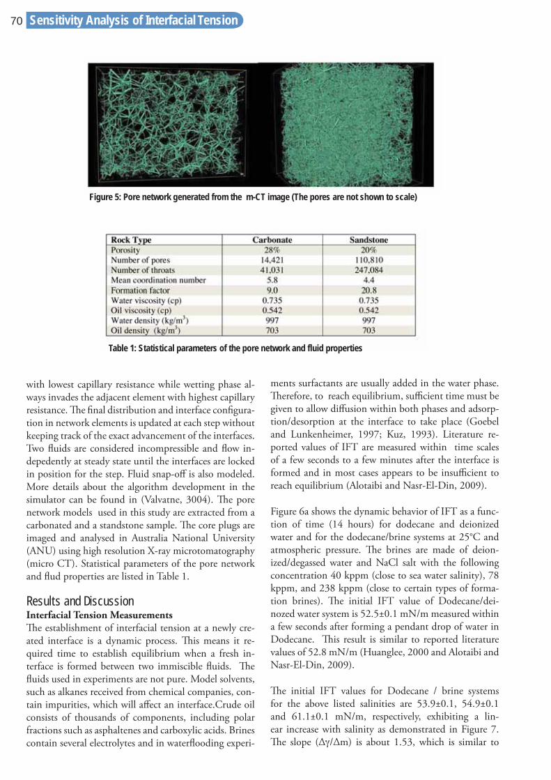
with lowest capillary resistance while wetting phase al-ways invades the adjacent element with highest capillary resistance. Th e fi nal distribution and interface confi gura-tion in network elements is updated at each step without keeping track of the exact advancement of the interfaces. Two fl uids are considered incompressible and fl ow in-depedently at steady state until the interfaces are locked in position for the step. Fluid snap-off is also modeled. More details about the algorithm development in the simulator can be found in (Valvatne, 3004). Th e pore network models used in this study are extracted from a carbonated and a standstone sample. Th e core plugs are imaged and analysed in Australia National University (ANU) using high resolution X-ray microtomatography (micro CT). Statistical parameters of the pore network and fl ud properties are listed in Table 1.
Results and Discussion Interfacial Tension Measurements Th e establishment of interfacial tension at a newly cre-ated interface is a dynamic process. Th is means it re-quired time to establish equilibrium when a fresh in-terface is formed between two immiscible fl uids. Th e fl uids used in experiments are not pure. Model solvents, such as alkanes received from chemical companies, con-tain impurities, which will aff ect an interface.Crude oil consists of thousands of components, including polar fractions such as asphaltenes and carboxylic acids. Brines contain several electrolytes and in waterfl ooding experi-
ments surfactants are usually added in the water phase. Th erefore, to reach equilibrium, suffi cient time must be given to allow diff usion within both phases and adsorp-tion/desorption at the interface to take place (Goebel and Lunkenheimer, 1997; Kuz, 1993). Literature re-ported values of IFT are measured within time scales of a few seconds to a few minutes after the interface is formed and in most cases appears to be insuffi cient to reach equilibrium (Alotaibi and Nasr-El-Din, 2009).
Figure 6a shows the dynamic behavior of IFT as a func-tion of time (14 hours) for dodecane and deionized water and for the dodecane/brine systems at 25°C and atmospheric pressure. Th e brines are made of deion-ized/degassed water and NaCl salt with the following concentration 40 kppm (close to sea water salinity), 78 kppm, and 238 kppm (close to certain types of forma-tion brines). Th e initial IFT value of Dodecane/dei-nozed water system is 52.5±0.1 mN/m measured within a few seconds after forming a pendant drop of water in Dodecane. Th is result is similar to reported literature values of 52.8 mN/m (Huanglee, 2000 and Alotaibi and Nasr-El-Din, 2009).
Th e initial IFT values for Dodecane / brine systems for the above listed salinities are 53.9±0.1, 54.9±0.1 and 61.1±0.1 mN/m, respectively, exhibiting a lin-ear increase with salinity as demonstrated in Figure 7. Th e slope (Δγ/Δm) is about 1.53, which is similar to
Figure 5: Pore network generated from the m-CT image (The pores are not shown to scale)
Table 1: Statistical parameters of the pore network and fluid properties
Sensitivity Analysis of Interfacial Tension70

Figure 6: Interfacial tensions of dodecane/brine systems with different salinities at 25°C and atmospheric pressure (A) 14 hours aging (B) 15 minutes magnification
Sensitivity Analysis of Interfacial Tension
what has been reported in literature for alkane/NaCl brine systems (Ikeda et al., 1991; Johansson and Eriks-son, 1974; Aveyard and Saleem, 1976). Ikeda et al. (Ike-da et al., 1991) measured IFT for Hexane/NaCl brine as a function of pressure and temperature for diff erent NaCl brine concentration and up to a molality of 1M, in both systems; he reported a slope of 1.54 (Δγ/Δm).
Looking at the impact of aging, it is apparent that even up to 14 hours the IFT still did not reach a clear equilib-rium. It is clear from these experiments that the changes
in IFT over time compared to the initial values are con-siderable, i.e. in the order of 33%. Note also in fi gure 7, that the increase in interfacial tension with salinity for measurements taken after 14 hours aging is consistent with but slightly larger than initial IFT results with a slope (Δγ/Δm) of 1.65.
Th e repeatable phenomenon observed here is a rapid drop in IFT within the fi rst seconds from forming the interface, followed by a slow decay (Figure 6). We be-lieve this is primarily due to the quick adsorption at
www.saudiarabiaoilandgas.com | SA O&G Issue 21
71
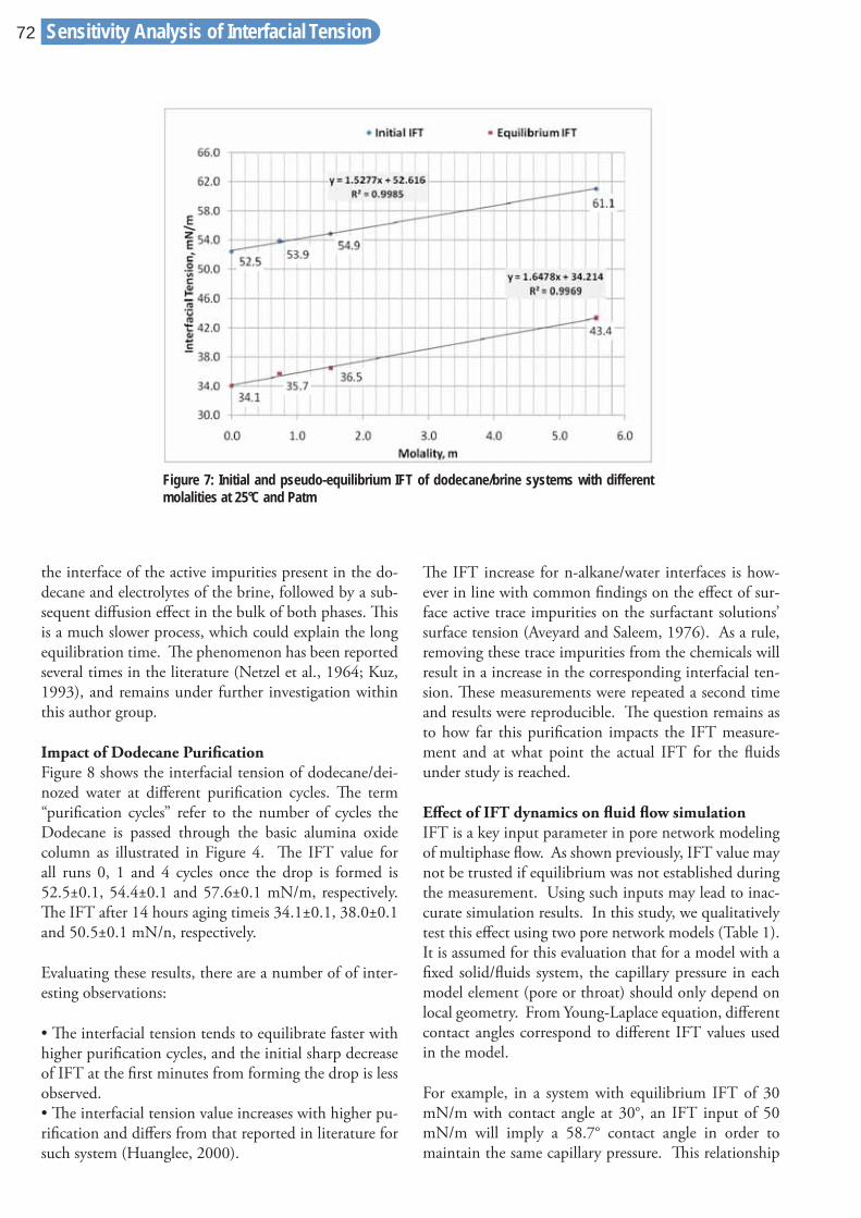
the interface of the active impurities present in the do-decane and electrolytes of the brine, followed by a sub-sequent diff usion eff ect in the bulk of both phases. Th is is a much slower process, which could explain the long equilibration time. Th e phenomenon has been reported several times in the literature (Netzel et al., 1964; Kuz, 1993), and remains under further investigation within this author group.
Impact of Dodecane Purifi cation Figure 8 shows the interfacial tension of dodecane/dei-nozed water at diff erent purifi cation cycles. Th e term “purifi cation cycles” refer to the number of cycles the Dodecane is passed through the basic alumina oxide column as illustrated in Figure 4. Th e IFT value for all runs 0, 1 and 4 cycles once the drop is formed is 52.5±0.1, 54.4±0.1 and 57.6±0.1 mN/m, respectively. Th e IFT after 14 hours aging timeis 34.1±0.1, 38.0±0.1 and 50.5±0.1 mN/n, respectively.
Evaluating these results, there are a number of of inter-esting observations:
• Th e interfacial tension tends to equilibrate faster with higher purifi cation cycles, and the initial sharp decrease of IFT at the fi rst minutes from forming the drop is less observed. • Th e interfacial tension value increases with higher pu-rifi cation and diff ers from that reported in literature for such system (Huanglee, 2000).
Th e IFT increase for n-alkane/water interfaces is how-ever in line with common fi ndings on the eff ect of sur-face active trace impurities on the surfactant solutions’ surface tension (Aveyard and Saleem, 1976). As a rule, removing these trace impurities from the chemicals will result in a increase in the corresponding interfacial ten-sion. Th ese measurements were repeated a second time and results were reproducible. Th e question remains as to how far this purifi cation impacts the IFT measure-ment and at what point the actual IFT for the fl uids under study is reached.
Eff ect of IFT dynamics on fl uid fl ow simulation IFT is a key input parameter in pore network modeling of multiphase fl ow. As shown previously, IFT value may not be trusted if equilibrium was not established during the measurement. Using such inputs may lead to inac-curate simulation results. In this study, we qualitatively test this eff ect using two pore network models (Table 1). It is assumed for this evaluation that for a model with a fi xed solid/fl uids system, the capillary pressure in each model element (pore or throat) should only depend on local geometry. From Young-Laplace equation, diff erent contact angles correspond to diff erent IFT values used in the model.
For example, in a system with equilibrium IFT of 30 mN/m with contact angle at 30°, an IFT input of 50 mN/m will imply a 58.7° contact angle in order to maintain the same capillary pressure. Th is relationship
Figure 7: Initial and pseudo-equilibrium IFT of dodecane/brine systems with different molalities at 25°C and Patm
Sensitivity Analysis of Interfacial Tension72

is shown in Figure 9. Since contact angle controls inter-face confi guration and thus fl uid distribution in model elements, diff erent fl ow scenarios can be expected. Ex-ample results of relative permeability curves using two pore networks are shown in Figure 10 and 11. Both fi gures show the eff ect on simulation results caused by feeding erroneous IFT value in the model, which results in a problematic interpretation of fl uid distribution and fl ow scenario. With only MICP data available, one can imagine that using non-equilibrium IFT value may lead to wrong contact angle calculation, which have signifi -cant impacts on relative permeabilities and residual oil saturations.
Although the aim of this study is not to model the eff ect of IFT reduction on sweeping effi ciency, it appears from both Figures 10 and 11 that reducing IFT from 50 to 30 mN/m shifts the normalized relative permeability curves to the left, suggesting reduced sweep effi ciency and the impact of modifying contact angle to normalized rela-tive permeability curves is overriding any recovery factor improvement by IFT reduction. Th is may be consist-ent with the accepted notion that a mixed wet system is more optimal from a water fl ood standpoint than ei-ther water or oil wet [Jadhunandan and Morrow, 1995; Kennedy et. al., 1955; Lorenz et. al., 1974].
In addition, the results of this simulation highlight the potential impact of this 20mN/m change in IFT from 50 to 30mN/m – in a transition zone where perhaps there is 40% water saturation, the oil relative perme-
ability is altered by a factor of 2 to 3. Th is can have marked consequences on development decisions when attempting to effi ciently recover oil with a water fl ood. It also greatly impacts the remaining saturations in these swept intervals.
Conclusions Interfacial tensions take a long time to equilibrate after interfaces are created. Diff usion, adsorption, and des-orption of impurities may cause interfacial tension to change with time and the nature of these impurities will aff ect further such equilibrium. When an interface is formed, the initial diff erences in concentration between the interface and the bulk phases act as the driving force of the system. Minute amounts of impurities present in experimental chemical fl uids “used as received” have a drastic impact on the properties of the interface. Results of pore network simulations imply that caution should be taken when IFT values are adopted in numerical models.
Th is all converges to addressing the question of fi eld sampled fl uid interfacial tensions. Crude oil contains many polar components that if not sampled or handled correctly will alter the results of IFT measurements. Pre-sumably within the formation the fl uids have reached a suitable “equilibrium”, and it is not obvious from our studies that the conventional methods for IFT measure-ment are replicating the downhole environment rigor-ously. Th e impact of inaccurate IFT; similar to fl uid properties or SCAL measurements; is clear when at-
Figure 8: Initial and pseudo-equilibrium IFT of dodecane / brine systems with different molalities at 25°C and Patm
Sensitivity Analysis of Interfacial Tension
www.saudiarabiaoilandgas.com | SA O&G Issue 21
73

tempting to build a fi eld development plan based upon reservoir simulations, and therefore demands attention.
Acknowledgement Th e authors would like to acknowledge Steve Dyer for his insightful discussion on the importance of such sub-ject to reservoir upscaling.
References Abdallah, W., Buckley, J.S., Carnegie, A., Edwards, J., Herold, B., Fordham, E., Graue, A., Habashy, T., Zeleznev, N., Signer, C., Hussien, H., Montaron, B., and Ziauddin, M., 2007. Fundamentals of Wettability, Oilfi eld Review 19(2): 44-61
Alotaibi, M.B., and Nasr-El-Din, H.A., 2009. Eff ect of Brine Salinity on Reservoir Fluids Interfacial Tension. SPE-121569, Presented at the 2009 EUROPEC/EAGE Annual Conference and Exhibition held in Amsterdam, Th e Netherland, June 8-11.
Anderson, W.G., 1987. Wettability Literature Survey – Part 5: Th e Eff ects of Wettability on Relative Perme-ability, J Petro Techno, 39: 1453-1468
Aveyard, R., and Saleem, S.M. 1976. Interfacial Tension at Alkane-Aqueous Electrolyte Interfaces, J Chem. Soc. Fara. Trans. I, 72: 1609-1617
Bakke, S. and Øren, P-E., 1997. 3-D Pore-Scale Mod-eling of Sandstones and Flow Simulation in the Pore Networks, SPE-35479. Presented at the European 3-D reservoir modeling conference held in Stavanger, Nor-way, April 16-17.
Bennion, D.B., Sarioglu, G., Chan, M.Y.S., Hirata, T., Courtnage, D., and Wansleeben, J., 1993. Steady-State Bitumen-Water Relative Permeability Measurements at Elevated Temperatures in Unconsolidated Porous Me-dia. SPE-25803, Presentaed at the International Th er-mal Operations Symposium held in Bakerfi eld, CA, U.S.A., February 8-10.
Goebel, A., and Lunkenheimer, K., 1997. Interfacial Tension of the Water/n-Alkane Interface, Langmuir, 13: 369-372
Huanglee, L., 2000. Th e gap between the measured and calculated liquid-liquid interfacial tensions derived from contact angles, J. Ad. Sci. Techno., 14(2): 167-185
Idowu, N.A. and Blunt, M.J., 2010. Pore-Scale Mod-eling of Rate Eff ects in Waterfl ooding. Transp Porois Med., 83: 151-169
Ikeda, N., Aratono, M., and Motomura, K., 1991. Th ermodynamics Study on the Adsorption of Sodium
Figure 9: Relationship between contact angles at different IFTs with a fixed capil-lary pressure
Sensitivity Analysis of Interfacial Tension74
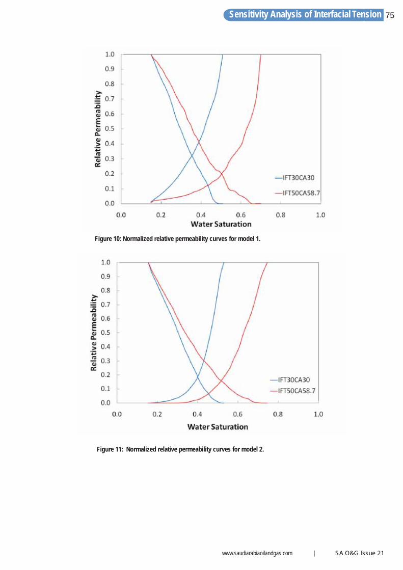
Figure 10: Normalized relative permeability curves for model 1.
Figure 11: Normalized relative permeability curves for model 2.
Sensitivity Analysis of Interfacial Tension
www.saudiarabiaoilandgas.com | SA O&G Issue 21
75

Chloride at the Water/Hexane Interface, J. Colloids. In-ter. Sci., 149(1): 208-215
Jadhunandan, P.P., and Morrow, N.R., 1995. Eff ect of Wettability on Waterfl ood Recovery for Crude-Oil/Brine/Rock systems, SPE-22597, Presented at the 1991SPE Annual Technical Conference and Exhibition held in Dallas, U.S.A., Oct. 6-9.
Janczuk, B. Wójcik, W. and Zdziennicka, A., 1993. Determination of the Components of the Surface Ten-sion of Some Liquids from Interfacial Liquid-Liquid Tension Measurements, J. Colloids Inter. Sci., 157(2): 384-393
Jasper, J.J., Nakonecznyj, M., Swingley, C.S., and Liv-ingston, H.K., 1970. Interfacial Tensions against Water of Some C10- C15 Hydrocarbons with Aromatic or Cy-cloaliphatic Rings, J. Phy. Chem., 74(7): 1535-1539
Johansson, K., and Eriksson, J.C., 1974. γ and dγ/dT measurements on aqueous solutions of 1,1-electrolytes, J. Colloids Inter. Sci., 49(3): 469-480
Kennedy, H.T., Burja, E.O., and Boykin, R.S., 1955. An investigation of the eff ects of wettability on the recovery of oil by waterfl ooding, J. Phys. Chem., 59:867-869
Koplik, J., Banavar, J.R., and Willemsen, J.F., 1989. Molecular dynamics of fl uid fl ow at solid surfaces, Phys-ics of Fluids A., 1: 781-794
Kovscek, A.R., Wong, H., and Radke, C.J., 1993. A pore-level scenario for the development of mixed wetta-bility in oil reservoirs, AIChE Journal, 39: 1072-1085.
Kuz, V.A., 1993. Th e aging of a Liquid Drop, Langmuir, 9: 3724-3727
Lorenz, P.B., Donaldson, E.C., and Th omas, R.D., 1974. Use of centrifugal measurements of wettability to
predict oil recovery, U.S. Bureau of Mines, Bartlesville Energy Technology Center, Report 7873.
Michaels, A.S., and Hauser, E.A., 1951. Interfacial ten-sion at elevated pressure and temperature. II Interfa-cial Properties of Hydrocarbon-Water Systems, J. Phy. Chem., 55(3): 408-421
Netzel, D.A., Hoch, G., and Marx, T.I., 1964. Adsorp-tion studies of surfactants at the liquid-vapor interface: Apparatus and method for rapidly determining the dy-namic surface tension, J. Colloid Sci., 19(9): 774-785
Swenson, P.D., Horvath-Szabo, G., Abdallah, W., and Eskin, D., 2011. A Novel Centrifugal Method for Wettability Characterization of Granulates, Ind. Eng.Chem. Res., Accepted for publication in February 15.
Shen, P., Zhi, B., Li, X.B., Wu, Y.S., 2006. Th e Infl uence of Interfacial Tesnion on Water/Oil Two-Phase Relative Permeability, SPE-95405 Presented at the SPE/DOE Symposium on Improved Oil Recovery held in Tulsa, Oklahoma, U.S.A, April 22-26.
Valvatne, P. and Blunt, M., 2004. Predictive pore-scale modeling of two phase fl ow in mixed wet media. Water Resour. Res., 407406.
Valvatne, P., 2004. Predictive pore-scale modeling of multiphase fl ow. PhD Dissertation, Earth Science and Engineering, Imperial College, UK.
Venturoli, M., and Boek, E.S., 2006. Two-dimensional lattice-Boltzmann simulations of single phase fl ow in a pseudo two-dimensional micromodel, Physica A., 362: 23-29.
Zhao, X; Blunt, M.J.; and Yao, J., 2010. Pore-Scale modeling: Eff ects of wettability on waterfl ooding oil re-covery, J. Petro. Sci. Eng., 71: 169-178
Sensitivity Analysis of Interfacial Tension76

UNITED KINGDOMAdam Mehar268 Bath Road, Slough, Berkshire,United Kingdom Main 44 1753 708872Fax 44 1753 725460Mobile 44 777 [email protected]
UNITED ARAB EMIRATESAbdul [email protected]: (971) 5056 8515
SAUDI ARABIAAkram ul HaqPO Box 3260, Jeddah [email protected]: (966) 557 276 426
Saudi Arabia Oil & Gas (Online) ISSN 2045-6689
Saudi Arabia Oil & Gas (Print) ISSN 2045-6670
For advertising, contact:
www.saudiarabiaoilandgas.com


Mr. Dave Clark Director, Dhahran Research and Technology Center, Baker Hughes, Saudi Arabia
Mr. Robert H. Gales Vice President, Unconventional Resources Projects, Weatherford
Dr. Nabeel Al Afaleq Manager, Northern Area Reservoir Management Department, Saudi Aramco
Mr. Darren Franklin Country Manager, Health, Safety, Environment & Operational Excellence Halliburton
Dr. Pacelli L. Zitha Delft University of Technology, The Netherlands
Dr. Amos Nur Director, Rock Physics & Borehole Geophysics, Stanford University, USA


Picture this: primeval man struggling to move a big kill or a great log. Carcasses of meat were no doubt hard to drag, but logs could be rolled and the invention of the wheel was not far off . Fast forward to the 21st century and witness the evolution of the wheel which is now entirely mechanised, powered by the internal combus-
tion engine and fueled by petroleum. While petroleum is not a ‘perfect’ fuel (it is fi nite and pollutes), the high density energy that is packed into every litre and the convenience with which it can be moved make it hard to beat. Th at is why it is not going away. Together, this triple combo – wheel, engine and petroleum – ranks
Exits from the Hydrocarbon Highway
‘Sometimes the best exitis the way we came in.’
Wajid Rasheed
www.hydrocarbonhighway.com www.eprasheed.com
“There have been many books concerning the oil industry. Most are technical, some historical (e.g. the Prize) and some about the money side. There are few, if any, about
the oil industry that the non-technical person will appreciate and gain real insight from. Wajid Rasheed in this book, The Hydrocarbon Highway, has made a lovely
pen sketch of the oil industry in its entirety. The book begins with the geology of oil and gas formation and continues with the technical aspects of E & P, distribution,
refining and marketing which are written in clear language. In particular, the process of oil recovery is outlined simply and with useful examples. There is a short history
of how the oil companies have got to where they are, and finally a discussion concerning the exits—alternative energy. This is all neatly bundled into 14 chapters
with many beautiful photographs and a helpful glossary. The book is intended to give an overture to the industry without bogging the reader down. I enjoyed the journey
along the highway.”
“I found the book excellent because it provides a balanced and realistic view of the oil industry and oil as an important source of energy for the world. It also provides
accurate information which is required by the industry and the wider public. Recently, I read several books about oil which portrayed it as a quickly vanishing energy source.
It seems that many existing books predict a doomsday scenario for the world as a result of the misperceived energy shortage, which I believe is greatly exaggerated
and somewhat sensational. Therefore the book bridges the existing gap of accurate information about oil as a necessary source of energy for the foreseeable future. The Hydrocarbon Highway should also help inform public opinion about the oil industry and our energy future. It looks at the oil industry in an up-to-date and integrated view
and considers the most important factors affecting it.”
Professor Richard Dawe of the University of West Indies, Trinidad and Tobago
Dr AbdulAziz Al Majed, the Director of the Centre for Petroleum and Minerals at the Research Institute at King Fahd University of Petroleum and Minerals
ISBN 978-0-9561915-0-2Price UK £29.95 US $39.95
“A crash course in Oil and Energy. The Hydrocarbon Highway is a much-needed resource, outlining the real energy challenges we face and potential solutions.”
Steven A. Holditch, SPE, Department Head of Petroleum Engineering, Texas A&M University
The Hydrocarbon Highway
By Wajid Rasheed
1
25/2/09 12:09:37
Hydrocarbon Highway84

among mankind’s greatest inventions and has rolled-out mankind’s greatest infrastructure endeavour, the Hydrocarbon Highway.
Our route along the Hydrocarbon Highway has shown that peak oil is not a physical shortage; there is plenty of untapped and unmapped oil. Moreover, technology is continually improving recovery.Consequently, peak oil is more of a psychological shortage. Our route has taken us behind the ‘Oil Curtain’ revealing the causes and eff ects of oil nationalism. We have seen how valu-able oil leases are acquired, developed and how ‘Extreme EP’ and intelligent wells are the future of production. Not least, we have considered renewable energy sources against the backdrop of carbon emissions and climate change. Before we reach our fi nal destination, ‘beyond petroleum’, we have to defi ne those scenarios and ‘ex-its’ to the highway where oil and gas can be practically replaced.
Plenty of signs jostle for our attention and some seem easy to take – do nothing, business as usual. Others re-quire complex questions to be considered: should more gas infrastructure be developed?; where should we build nuclear plants?; where should we dispose of nuclear waste?; what will compensate for shortfalls in renew-able power?; how should we store electricity eff ectively?; and, are biofuels causing food poverty? Tackling such diffi cult questions provides some insight into why there is so much dependence on hydrocarbons. We need to identify exits that are genuine and not those that just detour back to the hydrocarbon highway. Th is means fully thinking through where energy is supplied from and its end-use consumption (see Our Energy Future Images 1, above).
In order to move beyond petroleum, we need to under-
stand that there are no easy exits to hydrocarbon de-pendence; there is no silver bullet. Many so-called exits are still early prototypes ‘under construction’ requir-ing extensive research and development, political will, investment and time. It will take at least a generation before they become widely used. Still, each exit is ap-plicable in certain scenarios only. Not all countries wish to build or handle spent nuclear waste. Cold temperate climates do not lend themselves to solar power and wind power may not always be consistent. Not all countries can grow biofuels. Th e pivotal point is that no single energy source fi ts all needs.
All energy sources suff er from limitations related to fi t-for-purpose technicalities, start-up costs, output ef-fi ciency or societal trade-off s (see Our Energy Future Images 2). Any practical future energy scenario must include each and every one of these energy sources. Consequently, the answer lies in researching all options. Th at means experimenting and developing all applica-tions until we fi nd what works. Th e bottom line is that the Hydrocarbon Highway just got longer.
Gas Is the ‘New’ OilFrom all perspectives, gas emerges as one of the best po-tential exits from the Hydrocarbon Highway. If gas is a hydrocarbon though, how can it be an exit? Isn’t it just the same as oil being a fi nite fossil fuel? Gas is the best choice that we have as a bridge to the truly ‘renewable energy’ scenario as it can be man-made or naturally pro-duced and has low carbon emissions when burnt. Th e role of gas becomes clear in the energy models from the present period to the year 2030 which show that gas re-directs and eases off considerable demand for a broad number of oil applications1. Th e foundations for a ‘gas’ future have already been built using a broad set of ad-vanced gas2 technologies. Exemplifying this are Liquefi ed
Hydrocarbon Highway
www.saudiarabiaoilandgas.com | SA O&G Issue 21
85
Our Energy Future Images 1- Plenty of Signs Beckon But Where Do They Lead?

Natural Gas (LNG) which mobilises and commercialises stranded reserves. Additional examples are Compressed Natural Gas (CNG) and Liquefi ed Petroleum Gas (LPG) which provides fuel for the transport and power-genera-tion sectors through to Gas to Liquids (GTL) technol-ogy which off ers high quality gasoline fuel but at a high cost. Capping it all is renewable methane or man-made ‘bio-gas’ which is biologically produced. Gas is not a panacea though; it has limitations too.
So how much of a choice does gas or any other energy source really provide? Th at depends on whether the fuel can actually replace oil and how well it fi ts into future energy scenarios. In a major oil application such as avia-tion fuel, for example, gas in any form cannot replace oil due to engine design. Further complications exist as gas is not as easily transported as oil. It needs a specialised infrastructure to be developed which may be cost-eff ec-tive at a high oil price but not at a low one (see Figure 1).
Th e reason for considering all possible energy sources, and evaluating their strengths and weaknesses objective-ly, is to create a logic-based demand and supply equation for oil – one that qualifi es, future energy sources so that replacements can be identifi ed.
By asking whether oil can be replaced and whether the resulting carbon emissions are lower than those of oil, we can see just how far each energy source can really take us. Once they pass this qualifi cation stage, they can
then be fi tted into future energy trends allowing us to glimpse the future.
Summary: The MassesMost of today’s hydrocarbon dependence can theoreti-cally be ‘phased-out’ over the long term with renewable resources theoretically ‘phased in’ by 2050. Th is cannot happen in the short or medium term because replace-ments for oil do not off er straight oil swaps in mass; they are only usable in minute niches contributing to less than 5% of total oil energy demand worldwide. In contrast, 90% of oil and natural gas consumption is concentrated in trillions of transactions3. Th is vast consumption is most visibly spread worldwide among fl eets of cars, planes, trains and specialised machinery and equipment.
In order to appreciate the vast scale involved, imagine reconfi guring every gasoline station in your home town or city, in the state itself, the country, the continent and the world. Th en think about the network of distribu-tion and storage behind the retail outlets. Th at would represent half the equation – supply side only. Th e con-sumption side consisting of the engines that power the world’s fl eet of cars, trucks and buses would need to be reconfi gured too. Imagine doing the same for aviation, maritime and rail transport. Th ere is demand in oth-er components that would need to be considered too. Imagine reconfi guring existing power generation and industrial processes. Th e mass automotive and aviation products and mass processes such as power-generation
Hydrocarbon Highway86
Our Energy Future Images 2 - All Energy Sources Have Limitations Therefore We Need All Options

plants and petrochemical feedstock are confi gured for oil and natural gas usage; they are extremely diffi cult to change. In the short run, not much changes because of the demand inelasticity; however, in the medium term, a growing number of gas-based technologies, as well as growing volumes of ethanol and biodiesel can replace oil in mass products and mass processes*. Not only does this strengthen investment in the infrastructure and us-age of gas, ethanol and biodiesel but this also acts as a safety valve to dampen the demand for oil, redirect the excess demand from oil to gas and ultimately to the de-velopment of renewable resources.
Th is allows the next generation of new mass products and mass processes to be designed using gas, GTL, bi-odiesel, ethanol or co-generation while allowing the ex-isting infrastructure to be reconfi gured. In the long run, this acts as an exit as greater oil and gas demand elastic-ity is achieved overall 4.
Energy Consumption ModelsPrincipally developed by governments, energy compa-nies and universities, energy models seek to map out trends in future energy consumption. Many variants ex-ist, but essentially models are geared to low, medium and high levels of population, economic and demand growth. Salient trends are identifi ed and drawn up as scenarios allowing organisations to better handle poten-
tial future risk and opportunity. Corporate models are generally kept confi dential due to their commercial na-ture, while certain state and academic models are pub-licly available5.
US EIA/IEO Reference Case to 2030For our purposes, the US Energy Information Administration (EIA) or International Energy Outlook (IEO) reference case was selected as a global model for future energy consumption*. Considered by the US EIA to be the ‘business as usual’ future scenario, the IEO2008 reference case estimates world energy demand and supply to the period ending 2030. It at-tributes principal energy supply from oil, gas, coal, nu-clear and hydroelectric sources and separates the con-sumption of energy into the categories of transport, industrial, residential and commercial usage. Total glo-bal energy demand is estimated to increase by 50% from 462 quadrillion Btu to 695 quadrillion Btu in 2030 (see Figure 2). Th is is mostly driven by sustained consumer demand in the Organisation for Economic Co-opera-tion and Development (OECD) and industrial growth in Brazil, Russia, India and China (the ‘BRIC’s) (see Figure 3). World Gross Domestic Product (GDP) and primary energy consumption also grows more rapidly in the fi rst half than in the second half of the projections, refl ecting a gradual slowdown of economic growth in non-OECD Asia. Th e model envisages sustained high
Hydrocarbon Highway
www.saudiarabiaoilandgas.com | SA O&G Issue 21
87
Figure 1 - Higher oil price expands biofuels, unconventional oil, EOR and opens new frontiers (Source Booz Allen Haminton/IEA/Petrobras—Assumed average vs. marginal costs; 10% return for convention-al and 13% return for unconventional technologies; no subsides for biofuels; no carbon offset costs; after severance and production taxes.
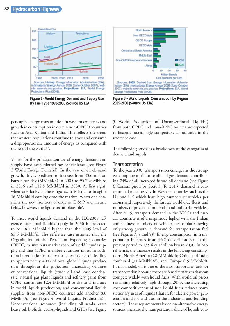
per capita energy consumption in western countries and growth in consumption in certain non-OECD countries such as Asia, China and India. Th is refl ects the trend that western populations continue to grow and consume a disproportionate amount of energy as compared with the rest of the world6,7.
Values for the principal sources of energy demand and supply have been plotted for convenience (see Figure 2 World Energy Demand). In the case of oil demand growth, this is predicted to increase from 83.6 million barrels per day (MMbbl/d) in 2005 to 95.7 MMbbl/d in 2015 and 112.5 MMbbl/d in 2030. At fi rst sight, when one looks at these fi gures, it is hard to imagine 16 MMbbl/d coming onto the market. When one con-siders the new frontiers of extreme E & P and mature fi elds, however, the fi gure seems plausible8.
To meet world liquids demand in the IEO2008 ref-erence case, total liquids supply in 2030 is projected to be 28.2 MMbbl/d higher than the 2005 level of 83.6 MMbbl/d. Th e reference case assumes that the Organisation of the Petroleum Exporting Countries (OPEC) maintain its market share of world liquids sup-ply, and that OPEC member countries invest in addi-tional production capacity for conventional oil leading to approximately 40% of total global liquids produc-tion throughout the projection. Increasing volumes of conventional liquids (crude oil and lease conden-sate, natural gas plant liquids and refi nery gain) from OPEC contribute 12.4 MMbbl/d to the total increase in world liquids production, and conventional liquids supplies from non-OPEC countries add another 8.6 MMbbl/d (see Figure 4 World Liquids Production) . Unconventional resources (including oil sands, extra heavy oil, biofuels, coal-to-liquids and GTLs [see Figure
5 World Production of Unconventional Liquids]) from both OPEC and non-OPEC sources are expected to become increasingly competitive as indicated in the reference case.
Th e following serves as a breakdown of the categories of demand and supply.
Transportation To the year 2030, transportation emerges as the strong-est component of future oil and gas demand contribut-ing 74% of all increased future oil demand (see Figure 6 Consumption by Sector). To 2015, demand is con-centrated most heavily in Western countries such as the US and UK which have high numbers of vehicles per capita and respectively the largest worldwide fl eets and numbers of private, commercial and industrial vehicles. After 2015, transport demand in the BRICs and east-ern countries is of a magnitude higher with the Indian and Chinese numbers of vehicles per capita showing only strong growth in demand for transportation fuel (see Figures 7, 8 and 9)9. Energy consumption in trans-portation increases from 93.2 quadrillion Btu in the present period to 135.4 quadrillion btu in 2030. In bar-rel terms, the increase results in the following consump-tions: North America (28 MMbbl/d); China and India combined (31 MMbbl/d); and, Europe (15 MMbl/d). In this model, oil is one of the most important fuels for transportation because there are few alternatives that can compete widely with liquid fuels. With world oil prices remaining relatively high through 2030, the increasing cost-competitiveness of non-liquid fuels reduces many stationary uses of liquids (that is, for electric power gen-eration and for end uses in the industrial and building sectors). Th ese replacements based on alternative energy sources, increase the transportation share of liquids con-
Hydrocarbon Highway88
Figure 3 - World Liquids Consumption by Region 2005-2030 (Source US EIA)
Figure 2 - World Energy Demand and Supply Use By Fuel Type 1990-2030 (Source US EIA)

Hydrocarbon Highway
www.saudiarabiaoilandgas.com | SA O&G Issue 21
89
Figure 5 - World Production of Unconventional Liquids 2005-2030 (Source US EIA)
Figure 4 - World Liquids Production 1990-2030 (Source US EIA)
Figure 6 - World Liquids Consumption by Sector 2005-2030 (Source US EIA)
Figure 7 - Transportation Liquids Consumption 2005-2030 (Source US EIA)
Figure 8 - Motor Vehicle Ownership in OECD Countries 2005, 2015 and 2030 (Source US EIA)
Figure 9 - Motor Vehicle Ownership in Non-OECD Countries 2005, 2015 and 2030 (Source US EIA)
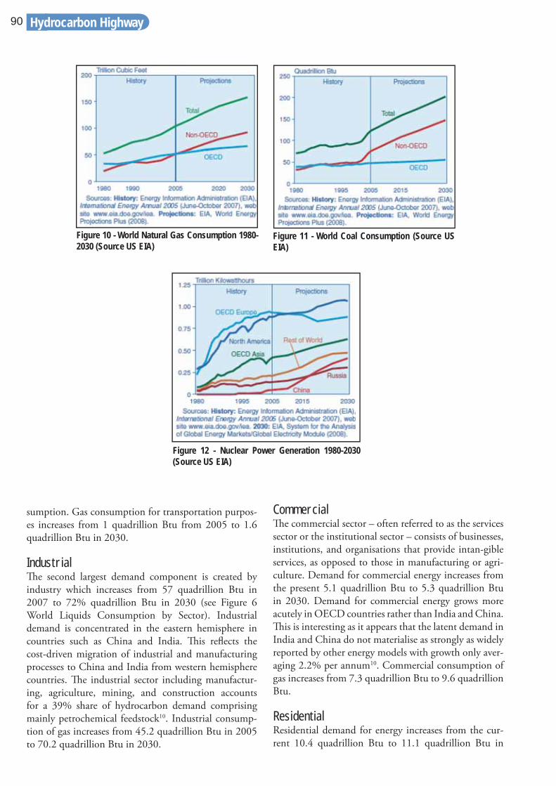
sumption. Gas consumption for transportation purpos-es increases from 1 quadrillion Btu from 2005 to 1.6 quadrillion Btu in 2030.
IndustrialTh e second largest demand component is created by industry which increases from 57 quadrillion Btu in 2007 to 72% quadrillion Btu in 2030 (see Figure 6 World Liquids Consumption by Sector). Industrial demand is concentrated in the eastern hemisphere in countries such as China and India. Th is refl ects the cost-driven migration of industrial and manufacturing processes to China and India from western hemisphere countries. Th e industrial sector including manufactur-ing, agriculture, mining, and construction accounts for a 39% share of hydrocarbon demand comprising mainly petrochemical feedstock10. Industrial consump-tion of gas increases from 45.2 quadrillion Btu in 2005 to 70.2 quadrillion Btu in 2030.
CommercialTh e commercial sector – often referred to as the services sector or the institutional sector – consists of businesses, institutions, and organisations that provide intan-gible services, as opposed to those in manufacturing or agri-culture. Demand for commercial energy increases from the present 5.1 quadrillion Btu to 5.3 quadrillion Btu in 2030. Demand for commercial energy grows more acutely in OECD countries rather than India and China. Th is is interesting as it appears that the latent demand in India and China do not materialise as strongly as widely reported by other energy models with growth only aver-aging 2.2% per annum10. Commercial consumption of gas increases from 7.3 quadrillion Btu to 9.6 quadrillion Btu.
ResidentialResidential demand for energy increases from the cur-rent 10.4 quadrillion Btu to 11.1 quadrillion Btu in
Hydrocarbon Highway90
Figure 10 - World Natural Gas Consumption 1980-2030 (Source US EIA)
Figure 11 - World Coal Consumption (Source US EIA)
Figure 12 - Nuclear Power Generation 1980-2030 (Source US EIA)

2030. Demand for energy consumption grows most in non-OECD countries in the residential sector at an average of 2.7%. Residential gas consumption in-creases from 19.1 quadrillion Btu to 25.2 quadrillion Btu11.
GasConsumption of natural gas worldwide almost doubles from 104 trillion cubic feet (tcf ) in 2005 to 158 tcf in 2030 as per the IEO2008 reference case (see Figure 10). Although natural gas is expected to be an important fuel source in the electric power and industrial sectors, the annual growth rate for natural gas consumption is slightly lower than the projected growth rate for coal consumption. Higher world oil prices in the IEO2008 increase the demand for and price of natural gas, mak-ing coal a more economical fuel source in the projec-tions. Industry accounts for the largest component of natural gas demand worldwide, generating 52% of the total growth in natural gas use in IEO projec-tions. Natural gas also provides the power generation sector with increasing supply and accounts for 39% of the increase in global natural gas demand to 203012.
Coal In the IEO2008 reference case, world coal consumption
increases by 65 percent over the projection period, from 122.5 quadrillion Btu in 2005 to 202.2 quadrillion Btu in 2030 (see Figure 11). Th e increase in coal consump-tion averages 2.6 percent per year from 2005 to 2015, then slows to an average of 1.7 percent per year from 2015 to 203013.
Nuclear PowerElectricity generation from nuclear power is projected to increase from about 2.6 trillion kilowatthours in 2005 to 3.8 trillion kilowatthours in 2030, (see Figure 12). Th is is based on rising fossil fuel prices, concerns regarding energy security and greenhouse gas emissions which tend to support new and existing nuclear power generation14.
Renewables Renewables including hydroelectric power (and other generating capacities fueled by renewable energy re-sources) are projected to increase by 352 billion kilowatt hours from 2007 to 728 billion kilowatt hours in 2030, at an average annual rate of 3.2%15.
Hydrocarbon Demand Supply EquationTh e IEO reference case is a very useful map to under-
Hydrocarbon Highway
www.saudiarabiaoilandgas.com | SA O&G Issue 21
91
Table 1 - Approximate Heat Content of Petroleum Products Million Btu (MMBtu) per Barrel
stand the direction of future energy. It still requires sys-tematic treatment and evaluation of specifi c renewable energy sources as well as oil-price dynamics which are non-linear. Its approach, however, is a very good basis from which to consider global energy markets, oil and gas segments and how mass transactions fi t in the overall picture. Th e oil and gas demand supply equation serves this purpose by outlining the six major oil and gas ap-plications and the twenty-one uses (mass products/mass processes) that result in mass transactions. Th is serves to pinpoint exit scenarios where oil and gas demand can be phased using an energy resource that is renewable. Th e value of the exercise lies in qualifying what is technically replaceable given an economic framework, i.e. high oil prices or government subsidies rather than calculating the economic or market value of each replacement.
What emerges from the analysis is an extremely broad and complex set of oil and gas applications and ultimate uses or transactions. Th ese range from transportation, to power generation, heating, petrochemicals, lubricants and surfacing. It was necessary to detail each specifi c end usage in order to determine whether oil and gas were replaceable commodities.
Th is is a key step in achieving higher elasticity of de-mand by satisfying end usage with replacement options. We assume that the production of petroleum will peak and then plateau, but that the broad range of petroleum applications that we see today will narrow down to a few that cannot be substituted by gas or other renewables.
Today, the only oil application that cannot be substi-tuted given the necessary economic framework, i.e. high oil prices or government subsidies, is aviation fuel which generates 5.7 million Btu per barrel compared to etha-nol which generates 3.5 million Btu. Aviation fuel then takes up approximately 0.61 times the volume of jet kero or it has 0.61 of the Btu17.
Firstly, there are six major categories of petroleum ap-plications which are split into a further 21 sub-catego-ries all of which have been kept as broad as possible, i.e. derivatives are split into Alkanes, Alkenes and Arenes which cover demand for derivatives such as plastics and pharmaceuticals.
Secondly, successfully substituting oil and gas depends on several unpredictable factors. Th ese include global economic stability in order to maintain oil prices above certain levels. Each alternative energy source has a corre-sponding oil price threshold at which it becomes profi t-able – or not – to pursue R & D. Th at threshold is not
simple to calculate; for example, in the case of bioetha-nol, it may be considered that an oil price of US $40 to US $60 per barrel makes ethanol production viable, but this does not take into consideration government inter-vention in the form of subsidies or incentives that are hidden away from ethanol or biofuel production. It is worth remembering that all biofuels are subject to sea-sonal conditions required for harvest. Unpredictable events such as inclement weather, hurricanes or market speculation can distort the acceptance curve of renewa-bles, accelerating or delaying the overall uptake18.
Th irdly, on a macro level there are no consensual fi gures on global consumption versus production data from ma-jor authorities. Much credit should go to BP for putting the statistical review together. Regarding country and global data, the issue is that ultimately all collating or-ganisations must rely on country export data as they have no way of verifying that data. Th e statistics there-fore incorporate OPEC/OGJ (Oil and Gas Journal)/non-OPEC data and so on. Th e approach has been to use regional or local data sources wherever possible.
Further discrepancies between consumption and pro-duction data exist from the same source; for example, the BP statistical review 2008 places global oil production at 81.53 MMbbl/d and consumption at 85.22 MMbbl/d. According to the BP statistical review, there is a defi cit of oil and a surplus of gas. Th e standard and fundamentally sound explanation for this discrepancy is explained by fuel additives, refi nery gains, measurement and round-ing up diff erences, inventories, etc. Th e discrepancy may also be partially explained due to illicit production not reported at the well-head, GTL production of liquids, gasifi cation and liquids from coal19. Another challenge with the data is conversion between physical volumes and oil equivalent volumes. Th e US EIA includes vol-ume adjustments to the production side so that produc-tion and consumption balance. Th e implicit assumption is that stocks don’t change.
Beyond PetroleumAs we look through the demand/supply equation it is apparent that it will take many years to provide other choices beyond petroleum. Indeed, oil may not be com-pletely replaced; rather, other choices will be off ered that have their own set of costs, trade-off s and limitations. Natural gas has emerged as an energy bridge to nas-cent renewables. Liquefaction commercialises stranded reserves, while biologically produced methane off ers renewability. Capping it all, GTL off ers high quality gasoline. Others such as oil-fi red power generation can be replaced by gas, nuclear, hydroelectric, or other re-
Hydrocarbon Highway92

newables. Co-generation and biomass production proc-esses that create methane or ethanol also off er eff ective renewable solutions. Last but not least, bio-diesels can be created from vegetable seed oil via trans-esterifi cation to provide replacements for diesel usage20.
Th e US EIA sees real resource limits to vegetable seed oil conversion to diesel, however, gasifi cation of biomass and then conversion to diesel should have much more promise in terms of available volumes.
Th e early trend here, and that which accompanies other oil and gas applications, is that until a new broadly appli-cable fuel is found, oil and gas will remain the preferred source for global energy, against a backdrop of a myri-ad of developing energy sources. Th is diverse scenario – the energy inclusive model – exists in Brazil, India and Pakistan, albeit in a nascent form (see Figure 13 Electricity Generation in Brazil by Fuel and 14 overleaf Brazilian Fuel Options at the Pump). Th ese countries are already using advanced gas technologies and etha-nol. Most countries worldwide are at diff erent points of energy development, with emphasis on hydro-electric, nuclear or other renewables varying from country to country21.
2008 World Demand (Consumption)1. Gas 2921.9 Bm3. Th is fi gure is based on storage fa-cilities, liquefaction, the disparities with production are due to defi nition, measurement or conversion, proposed additional sources, fl aring and GTL22.
2. Oil 85.22 MMbbl/d. Th e diff erence in consumption and production is due to inventories, additives such as ethanol, stock changes, substitutes, measurement/con-
version, proposed additional sources, illicit production and GTL23.
2007 World Supply (Production)1. Gas: 2940 Bm3 which excludes GTL, Coal to Gas)24.
2. Oil 81.53 MMbbl/d which includes NGL and GTL production25.
For detail on the individual demand or supply compo-nents, refer to the Notes at the end of the book. Th e ma-jor categories are: transportation, heating, petrochemi-cals, lubricants, surfacing and power generation. Now let us look at the demand components and what choices we have for oil replacement.
Transportation (Aviation, Automotive,Marine and Rail)Replacements in high-demand areas of aviation, auto-motive and marine usage are limited. Choices exist, but they are tempered by engine type, fuel tank size*, up-grading retail outlets and upgrading existing automotive and marine fl eets. From the outset, the thermodynamic cycle and engine type – Otto or Diesel – dictates appli-cation suitability. Otto cycle engines use gasoline which can be replaced by ethanol. Diesel cycle engines use die-sel which can be replaced by biodiesel. Both are ideal for spark-ignition and compression-ignition engines.
Ethanol, the much vaunted ‘fl ex-fuel’, off ers only a par-tial exit scenario by substituting gasoline in the Otto cy-cle applications only. It is also fair to note that Brazil’s adoption of ethanol (and LPG) technologies took at least 30 years to achieve, with car manufacturers and oil com-panies creating the required infrastructure. Government
Hydrocarbon Highway
www.saudiarabiaoilandgas.com | SA O&G Issue 21
93
Figure 13 - Electricity Generation in Brazil by Fuel (Source US EIA)

legislation required 25% of all gasoline to be mixed with ethanol. Today, that percentage has fallen to 20% as de-mand (and exports) of ethanol rises. Ethanol does have its own supply volatility and liquidity limitations26.
Successful usage in one country, however, does not mean that global roll-out can occur. As Brazil is one of the most advanced in energy diversifi cation, what lessons can be drawn from its experience? First, government support was not enough; intervention was required. It was Brazil’s dictatorship in the 1970s that issued the di-rectives that led to today’s usage. More than 30 years of government intervention, manufacturing incentives, infrastructure and retail outlets were needed to reach the current ‘fl ex-fuel’ conditions of 5% of all fuel consumed and 100% of all nationally manufactured cars. Th e main obstacle to worldwide roll-out is that the existing fl eet of cars, buses, and boats around the world are confi gured for petroleum and diesel. Th is requires a phasing out or phasing in approach. Meanwhile, incentives or direc-tives for new build vehicles should ensure that they are confi gured for fl ex-fuel renewables27.
Th e Brazilian government has now applied the 5% min-imum usage target to bio-diesel. Th is requirement has a number of transport fuel implications. First, it is likely to create more demand for petroleum replacements or ‘un-conventional fuels’ as long as prices stay high. Second, more unconventional liquid fuels (GTLs, ethanol and biodiesel produced from alcohol or seeds) and natural gas (compressed or liquid) are likely to come onto the
market and take up a larger share of overall demand for transportation petroleum liquids to 2030. Over the short run, this can be considered as a safety valve that eases off demand for traditional oil fuels (gasoline and diesel) in the transport demand component. In the long run, it can be considered as a partial exit scenario28. Th e major part of demand, however, resides within transpor-tation and is highest in OECD countries such as the US, Canada and Western Europe. It is these countries that can help reduce demand by using more effi cient vehicles as well as sharing transportation. A good idea would be to provide tax incentives for fuel effi cient vehicles as well as car pooling.
Heating Similar obstacles face the stock of domestic dwellings in that they cannot easily be confi gured to use oil or replacement gas. Greater acceptance of renewable en-ergy sources (nuclear, solar, wind) can be expected in new-build residential usage. Natural gas (compressed or liquid) is also likely to take up a greater portion of total residential demand for petroleum. Over time, this can be considered another safety valve that eases off demand for traditional residential oil fuels (gas and diesel) in residential demand. Localised burning of any carbon-based fuel for residential heating creates considerable diffi culties. Firstly, establishing an effi cient distribution infrastructure to transport the fuel to the homes can be expensive, time-consuming and problematic. Secondly, the control and capture of CO2 (or other GHGs) is vir-tually impossible at the house-to-house level. Better to
Hydrocarbon Highway94
Figure 14 - Brazilian Options at the Pump 2009 shows Ethanol, Gasoline, Diesel and Natural Gas (EPRasheed)

provide 100% electrifi cation of communities, whereby carbon-based fuels are converted to electric energy at a few, centrally-located and controlled power stations where emissions can be controlled and GHGs seques-tered. Electric power grids are relatively easy to establish, expand and maintain. Electric energy is a much more versatile form of energy, capable of providing many more services from heating to cooling, to illumination, to cooking and to powering appliances of all sizes. It is truly the world’s cleanest and most easily-assimilated energy resource. Localised or dispersed burning sites would therefore be dramatically reduced, thus reduc-ing the carbon footprint. More unconventional liquid fuels (GTLs, ethanol and biodiesel produced from al-cohol or seeds respectively) and natural gas (compressed or liquid) are likely to come onto the market and take up a larger share of overall demand for commercial heat-ing petroleum liquids to 2030. Over time, this can be considered a partial exit for traditional heating oil fuels (kerosene, diesel, heavy oil) in the commercial demand component29.
Power GenerationWhat is important here is that each country’s energy needs and resource profi les diff er, and this aff ects how advanced (or not) their renewables uptake is and what size contribution it makes. It is clear to see that renew-ables off er a broad band of applications, concentrated in low-scale power generation, large scale gas turbine power generation or biomass co-generation applica-tions. Choices exist, but they are tempered by the power generation facility type. Gas turbine or combustion tur-bines use natural gas, light fuel oil, diesel or biologically produced gas.
Still, many limitations exist; for example, power gen-erating conditions for renewables do not always coin-cide with peak demands. Specifi c levels of sunshine or wind speed must exist at a given time to generate energy which must then be stored, creating a further challenge that must be resolved.
In the reference case, however, natural gas and renewable energy sources are predicted to increase in power genera-tion markets. Th e natural gas share of world electricity markets increases from 19% in 2003 to 22% in 2030, and the renewable share rises from 18% in 2003 to 20% in 2010 before declining slightly to 19% in 2030. Th e relative environmental benefi ts and effi ciency of natu-ral gas make the fuel an attractive alternative to oil and coal-fi red generation. Higher oil and gas prices enable renewable energy sources to compete more eff ectively in the electric power sector30.
PetrochemicalHigh petrochemical feedstock demand is likely to create more demand for reformulated or ‘syntheti-cally’ produced feedstocks. More synthetically pro-duced alkenes and arenes will be created from gas, GTL and ethanol. As these products come onto the market, they will contribute to meeting higher levels of demand from the petrochemical sector. Over time, this will tend to a partial exit scenario with pet-rochemical-based hydrocarbon demand taking up to a 60% share of industrial demand up to 2030.
Lubricants and SurfacingMore synthetic lubricants (reformulated or vegetable seed based) and surfacing products (cement type) are likely to come onto the market and take up a larger share of overall demand for lubricants and surfacing. Over time, this can be considered an exit for traditional lubricants and surfacing (heavy oils, asphaltene) in the commercial demand component.
Price and Alternate ScenarioAt any given point, the oil price is the closest, albeit im-perfect indicator, due to delay of how the demand/sup-ply equation is balanced. High oil and gas prices tend to indicate high demand and tight supply and vice versa. Th ere is a complex inter-play, but clearly high oil and gas prices have three major implications. First, energy at-tracts investment. Th is is because high oil prices awaken demand for all types of energy sources, not just oil. Th is is double edged as not only does oil attract investment so do renewables. Exemplifying this is coal and ethanol which reached record prices during 2008. In the case of agriculturally produced ethanol, the price of other agri-cultural crops can also increase as arable land is used for ethanol production. Given that the uptake of renewables is very sensitive to oil and gas prices, a 1.5% increase per annum in renewables uptake can help stabilise energy demand with oil production staying constant. Second, large reserve holders do increase E & P but not relative to the oil price. As the absolute value of oil increases, these countries reduce domestic consumption, encour-age substitutes and focus on maximising recovery from existing assets rather than producing from new fi nds. Th ird, high oil prices depress demand. Over time, all of this happens almost imperceptibly; pent up consump-tion for oil dissipates and demand for goods and services falls due to higher costs. It was incorrect thinking that suggested that high oil prices could be borne by econ-omies without greatly aff ecting growth. Th is has been proven time and again to be the downfall of high oil prices and the precursor to a bust cycle31.
Hydrocarbon Highway
www.saudiarabiaoilandgas.com | SA O&G Issue 21
95

It is diffi cult to predict oil prices because oil price cycles tend to perform in a complex almost chaotic manner. Oil, however, is a commodity and obeys market rules or fundamentals despite the distortions. Research focused on commodities and, although not specifi cally designed for oil, shows how commodity cycles are aff ected by in-ventory, immediate production capacity and long-term production capacity. Th e combination of diff erent times-cales, time delays, diff erent operators and human fallibil-ity only adds to the complexity of the system. Although cycles (peaks and troughs) are not entirely random, we know that they will occur. Th e length of each cycle (say from peak to peak) is not entirely predictable as some last three years while others can last as long as ten years. Th ere are, however, some telltale signs: economic condi-tions worldwide; extreme swings from a low to a high price or vice versa within a six month period; and, major geo-political tension. Prolonged periods of tightness in acquiring supply or services (or vice versa) also provide a good indication of where we are in the cycle.
Th e much touted increase in demand from China and India occurred in 2008 and is now slowing down. Th e growth in demand for energy is a much more gradual and long-term event linked to positive economic growth and consumption in developed countries. Combined demand from China and India exceeds North America by 2030, but not on a per capita energy usage basis. Th e bulk of Chinese and Indian industry and services are pro-duced for end consumption by foreign customers mostly in Western countries and North America. Consumption has been transferred to China and India to refl ect the industrial activity and production there. Endogenous demand for petroleum would be much lower without the energy consumption from traditionally high energy per capita users. Th e bulk of energy consumption, there-
fore, arises from the traditional users, i.e. in the US and Western Europe.
How long will the present recession last? Not even the world’s best economists can say. Without getting too much into economic theory, we can say that there will be a market correction: a collapse or a period of depressed demand and lower oil and gas prices. We know that is certain because oil and gas are cyclical commodities that periodically experience peaks and troughs32. Th e prob-lem is nobody knows when these will occur because the cycles are not entirely predictable; however, current mar-ket situations clearly seem to herald a low price cycle.
From a market perspective (putting government inter-vention aside), the troughs mean diminished demand for oil and gas and its applications, less cash for explo-ration and even less cash for renewable resources. Put simply, the return forecasts are lowered and the principal fl ow of capital from investors and speculators is diverted into markets other than energy and oil.
Nobody wants to talk about a collapse in prices. It frightens investors. Nobody wants to talk about a col-lapse when growth is strong, but ignoring a low price scenario is asking for trouble. Th is perhaps explains why oil companies want to stay cash rich. Th ey have lived through the low price scenario—low revenues, poor uti-lisation and even lower returns. Th is is what some say keeps the cycle of under investment alive—fear of price collapse33 (see Figure 15).
Our Legacy? Our task is to lobby for investment, both in oil and gas and R & D in renewables and to understand there is no easy way out. We will all have to work to fi nd an
Hydrocarbon Highway96
Figure 15 - Oil price 1861-2009. Source BP and EPRasheed (US, Arab Light and Brent Prices)

exit. What about an energy revolution? It may happen, but my money is on the evolution: experimenting and tinkering with all energy sources. And what of global warming and energy? Simply put, we must reduce car-bon emissions. Th ere are new kids on the block (e.g. ethanol and wind farms) and there are some old-timers back as well (e.g. nuclear and coal). I believe that in the future, energy will become a new engineering discipline, along with mining, civil, mechanical, petroleum and nuclear and one that encompasses wind, solar and all other forms of energy.
Th ink legacy. Th ink future generations. Do we want to leave a mess of energy waste and environmental dam-age as a legacy for future generations? What does that say about us? Together, we need to apply our minds to exit the Hydrocarbon Highway without leaving a mess behind us. So how will things look in the future?
Th e narrowing base of opportunities for IOCs due to a changing E & P landscape means their activities will tend toward gas (GTL, LNG) and renewables. Here IOCs take a leadership position by diff erentiating them-selves and adopting the ‘Inclusive Energy Model’ with project management, the know-how and capital. Gas becomes the fuel of choice from renewable streams, i.e. biomass as well as fossil fuel streams. Other applications are replaced, eff ectively relieving the major part of de-mand pressure on petroleum. Due to unreplaced appli-cations, seasonal events and die-hards, the Hydrocarbon Highway runs on. Renewables increase over time but do
not displace petroleum entirely creating an inclusive en-ergy model. Petroleum remains a permanent feature, its demand increasing from time to time as ethanol crops fall short or rainfalls fall below hydro-electric dam re-quirements (and just as people still warm to a log-fi re, people will always enjoy the thrill of gasoline powered revs).
Nuclear energy becomes a leading renewable energy source. Electricity prices rise, noticeably driven by the global rise in gas prices. As more nuclear energy plants come onstream, nuclear energy becomes more competi-tive and gas prices fall. Hydrocarbon demand is reduced by other factors too. Increasing GHGs and global warm-ing becomes a reality. Companies are sued for producing emissions. Th e cases are defended, but companies be-come the champions of levying carbon taxes on the gen-eration of GHGs. Th is is similar to the relationship be-tween obesity and fast food chains. Th e fast food chains avoided direct responsibility in lawsuits and learned the lesson to off er ‘healthy’ alternatives. Aviation prices rise; the industry is thrown into disarray. Cheap airlines are forced to consolidate and stress on petroleum aviation demand is lowered further. Oil prices continue to fl uc-tuate, yet a balance of residual demand keeps oil compa-nies in business. A fl ourishing trade in carbon miles exist at the state, corporate and individual level. Worldwide, those who do not use their allowances sell the diff erence to high users. Electrically charged cars run globally.
Gasoline stations are still aff ectionately known as
Hydrocarbon Highway
www.saudiarabiaoilandgas.com | SA O&G Issue 21
97
Figure 16 - Future Options at the Pump; The Energy Express (EPRasheed)

petrol or gas stations as a throwback to when petro-leum spirit was the dominant fuel, but they now off er biofuels, electricity, hydrogen and gasoline. Th e Hydrocarbon Highway has become the Energy Express. We have more choices than ever – the highway is still endless, but now there are many branching intersections one can take.
References1. Th ese are: a) Power Generation [PGOil +PGGasTurbine (Non Ethanol/Brighton cycle) +PGGasSteam (Combustion)] (Gasoil/Fueloil) Gas & Oil (Methane, Heavy Oil)
b) Heating [H Industrial Process + H Construction +H Domestic Premises +H Commercial Premises] (Gas, Kerosene, Gasoil)
c) Transport [T Light Automotive Cars + T Aviation + T Marine Light T Marine T Military T Industrial + T Heavy Automotive Truck/Construction/Mining T Heavy Automotive Bus +T Train] (Gasoline, Diesel, Heavy Oil)
d) Petrochemicals [D Alkane Feedstocks (Naphthas) + D Arene Feedstocks (Pharmaceuticals) + D Alkene Feedstocks Plastics + D Foods + Resins & Waxes]
e) Lubricants [L GearOil + L IndustrialGrease], and
f ) Surfacing [S Road+S Roof ] Roofs, Cement.
2. Especially considering man-made Gas.
3. Th at make up the Oil and Gas Demand Equation: [PGGT+PGGS+PGO]+[HIP++HCon+HDP+HCP]+[TLAC+ TA + T M+ THAT+THAB+TT]+ [PCArF (Pharmaceuticals) + PC AlF PC AlkeneF + PC RW] + [LGO + LIG] + [SRd+SRf ] 2007 World Demand (Consumption) Gas 2921.9 BCM and Oil 85.22 mil-lion bopd 2007 World Supply (Production) Gas: 2940 BCM and Oil 81.53 million.
Supply = [PGMethaneGT +PG MethaneGS+LPG,LNGGS + PG Oil] + [HGasOilIP+HGasDP Diesel, CNG,LPG ] +[TLAC Gasoline+ Diesel + TA Compressed Natural Gas, Liquid Petroleum Gas + TM Diesel+ THAT Diesel+THAB Diesel+TT Heavy Oil ] + [PCArF Naphtha (Pharmaceuticals) + PC AlF Naphtha PC AlkeneFNaphtha + PC RW Heavy Oil] +[LGOHeavy Oil + LIGHeavy Oil] + [SRdAsphalt+SRfBitumen].
4. Th is is our goal.
5. See EIA IEO 2008 Outlook.
6. See EIA IEO 2008 Outlook.
7. Idem.
8. Idem.
9. Certainly the EIA IEO 2008 Outlook thinks so.
10. EIA.
11. EIA.
12. EIA.
13. Idem.
14. Idem.
15. EIA.
16. EIA Footnote.
17. Increasing Feedstock Production for Biofuels: Economic Drivers, Environmental Implications, and the Role of Research. See also Options for Alternative Fuels and Advanced Vehicles in Greensburg, Kansas Harrow, G.
18. Further is the intrinsic volatility of the oil markets which complicates investment in renewables.
19. Exchange with EIA.
20. Exchange with EIA.
21. Brazil is a case in point hence why it was chosen.
22. BP Statistical Review 2008.
23. Idem.
24. Idem.
25. Gasoline and Ethanol Prices Fall” (in Portuguese). Folha Online 18 09 2008.
26. US DOE Flexible Fuel Vehicles: Providing a Renewable Fuel Choice. Again no single source of en-ergy is universally applicable.
27. See also Th e Methanol Story: A Sustainable Fuel for the Future Roberta J Nichols.
28. US DOE Flexible Fuel Vehicles: Providing a Renewable Fuel Choice.
29. In many ways this is more elastic than transporta-tion demand.
30. It is the backdrop of high oil prices that makes re-newables viable.
31. Th e trends for continued economic and population growth will create further demand on oil and gas in the medium and long term.
32. Th e problem is that not even the world’s foremost thinkers can satisfactorily predict the cycles.
33. Due to the vicious cycle involved it is likely that change will be slow and steady.
Hydrocarbon Highway98

Jan/Feb Mar/Apr May/Jun Jul/Aug Sep/Oct Nov/Dec
* Saudi AramcoSupplement
Editorial 2011 Calendar
Contribute to Saudi Arabia Oil & Gas during 2011
BONUS CIRCULATION
SPECIAL PUBLICATIONS
www.saudiarabiaoilandgas.com
• Saudi Aramco RTOC
• Digitalization
• While DrillingTechnology
• Telemetry
• Production
• OGEP II Review
• Khurais
• Near SurfaceModelling
• Rotary Steerable &Motor Systems
• Drill Bits and Under-reamers
• Complex Wells
• Geophysical
• Drill Pipe Integrity
• Manifa• Remote Operation Centre• Drill-Bit Tech• Inflow Control Devices• Zonal Isolation (incl. Packers,Multi-ZoneCompletions)• Carbonate ReservoirHeterogenity • Exploration Rub Al Khali
• Formation Evaluation
• Wellbore
Intervention
• Casing While Drilling
• Multi-Laterals
• Lowering Drilling Costs in Tight Gas
• Evaluating Tight Gas Formations
•Increasing Productivity of Tight and Shale Gas
• Khursaniyah
• ExpandableCompletions
• Tubulars
• Logging and
Measurement WD
• Electrical
Submersible Pumps
• ProgressiveCavity Pumps
• Novel Tight Gas Technologies
• Hawiyah
• Smart Completions
• I field
• Geosteering
• GOSP
• Extended Seismic Feature (4D, OBC, Wide Azimuth)
EPRasheed is looking for editorial submissions on the topics outlined in the editorial calendar. This can provide your company with the opportunity to communicate EP technology to the wider oil and gas community.
Please send abstracts or ideas for editorial to [email protected]
Preference is given to articles that are Oil Company co-authored, peer reviewed or those based on Academic research.
SPE/IADC Drilling Conference1-3 March 2011AmsterdamThe Netherlands
Royal Commission for Yanbu and Jubail Saudi Downstream* 8-9 March 2011
YP Symposium**14-16 March 2011
Middle East Oil and Gas Show andConference*20-23 March 2011 ManamaBahrain
9th Meeting of the Saudi Society for Geosci-ences** 26-28 April, 2011 King Saud University Campus, Riyadh
Offshore Technology Conference2-5 May 2011Houston, Texas, USA
SPE/DGS AnnualTechnical Symposium &Exhibition*15-18 May 2011 Khobar, Saudi Arabia
73rd EAGE Conference &Exhibition/SPE EUROPEC23-26 May 2011Vienna, Austria
Brasil OffshoreExhibitionConference14-17 June 2011Macae, Brazil
Offshore Europe*6-8 Sept 2011Aberdeen, UK
SPE/EAGEReservoirCharacterization and Simulation Conference26-28 Sept 2011Abu Dhabi, UAE
OTC Brasil4-6 Oct 2011Rio de Janeiro, Brazil
Middle EastDrilling Technology Conference andExhibition24-26 Oct 2011Muscat, Oman
SPE Annual Technical Conference and Exhibition30 Oct - 2 Nov 2011DenverColorado, USA
InternationalPetroleumTechnologyConference15-17 Nov 2011Bangkok, Thailand
20th WorldPetroleumCongress*4-8 December 2011Doha, Qatar
* Offi cial Saudi Magazine
** Offi cial Magazine
* Offi cial Technical Magazine* Media Partner** Offi cial Technical Magazine
* Media Partner
Ad Closing:4 Jan 2011Materials Closing:11 Jan 2011
Ad Closing:1 March 2011Materials Closing:4 March 2011
Ad Closing:22 April 2011Materials Closing:29 April 2011
Ad Closing:5 July 2011Materials Closing:12 July 2011
Ad Closing:29 August 2010Materials Closing:30 August 2011
Ad Closing:8 October 2011Materials Closing:15 October 2011
Issue 18 ‘OGEP II Review’
Issue 19‘Innovation, IOC, NOC and Service CompanyAlliances’
Issue 20‘Upstream Challenges’
Issue 21‘Tight Gas Lowering Costs and Increasing Productivity’
Issue 22‘Cost Effective Drilling and Completions’
Issue 23‘Cooperation, Innovation and Investment’

*Mar
k of
Sch
lum
berg
er.
Mea
sura
ble
Impa
ct is
a m
ark
of S
chlu
mbe
rger
. ©
201
0 S
chlu
mbe
rger
. 0
9-S
T-01
50
Introducing HiWAY* channel fracturing— A new hydraulic fracturing technique that creates flow channels to maximize the
deliverability of the reservoir.
With this technique, there’s nothing between the reservoir and the well, so reservoir
pressure alone determines flow.
Open up. No speed limits.
www.slb.com/HiWAY
Global Expertise | Innovative Technology | Measurable Impact
Experience infinite fracture conductivity FLOW-CHANNEL
HYDRAULIC FRACTURING TECHNIQUE
HiWAY
Conventional fracturing HiWAY channel fracturing