Ground water evaluation and coolingbefore utilization for Wadi Zam-Zam, Libya

Item Type Thesis-Reproduction (electronic); text

Authors Jarroud, Omar Ali,1946-

Publisher The University of Arizona.

Rights Copyright © is held by the author. Digital access to this materialis made possible by the University Libraries, University of Arizona.Further transmission, reproduction or presentation (such aspublic display or performance) of protected items is prohibitedexcept with permission of the author.

Download date 14/07/2018 01:23:25

Link to Item http://hdl.handle.net/10150/191656

GROUND WATER EVALUATION AND COOLING BEFORE

UTILIZATION FOR WADI ZAM-ZAM, LIBYA

by

Omar Ali Jarroud

A Thesis Submitted to the Faculty of the

DEPARTMENT OF HYDROLOGY AND WATER RESOURCES

In Partial Fulfillment of the RequirementsFor the Degree of

MASTER OF SCIENCEWITH A MAJOR IN HYDROLOGY

In the Graduate College

THE UNIVERSITY OF ARIZONA

1977

STATEMENT BY AUTHOR

This thesis has been submitted in partial fulfillment of require-ments for an advanced degree at The University of Arizona and is depos-ited in the University Library to be made available to borrowers underrules of the Library.

Brief quotations from this thesis are allowable without specialpermission, provided that accurate acknowledgment of source is made.Requests for permission for extended quotation from or reproduction ofthis manuscript in whole or in part may be granted by the head of themajor department or the Dean of the Graduate College when in his judgmentthe proposed use of the material is in the interests of scholarship. Inall other instances, however, permission must be obtained from theauthor.

SIGNED:

APPROVAL BY THESIS DIRECTOR

This thesis has been approved on the date shown below:

D. D. EVANS DateProfessor of Hydrology and

Water Resources

To my mother

ACKNOWLEDGMENTS

I am deeply thankful to my family, their constant encouragement

and moral support have made this thesis a reality.

I am grateful to Dr. Daniel D. Evans, who supervised my graduate

work, for his encouragement, patience, and advice.

Dr. Rocco A. Fazzolare generously gave of his time to advise me

on various aspects of my thesis. I wish to thank Dr. K. James DeCook and

Dr. Simon Ince, members of my committee, for their interest in the

progress and subject matter of my thesis.

Special thanks are given to Non i Esbak and the Libyan General

Water Authority staff for their assistance in collecting data by

supplying valuable information and equipment.

I wish to extend thanks to the Wadi Zam-Zam Project Authority for

the gracious hospitality expressed while allowing me to collect essential

measurements.

Special appreciation is given to Christine C. Milsud for sugges-

tions in improving the manuscript and plotting some graphs.

iv

TABLE OF CONTENTS

Page

LIST OF ILLUSTRATIONS vii

LIST OF TABLES xi

ABSTRACT xii

I. INTRODUCTION 1

The Problem 2Scope of the Investigation 3

2. GROUND WATER EVALUATION 4

Background 4Location and Extent of the Area 4Climate 6Topography 9Natural Resources and Population 9Previous Investigation 12

Geology 14Quaternary 15Eocene 15Paleocene 20Cretaceous 20

Ground Water 22Aquifers 22

Characterization of Chicle Sandstone Aquifer 24Extent of the Aquifer 24Discharge and Movement 25Recharge to Ground Water 26Transmissivity and Storage Coefficient 26Interference Effect within the Well Field 28Piezometric Head 30

Well Specifications 38Artesian Head and Discharge 38Well Spacing 4o

Well Design 42Estimating Head Losses Inside the Well 45

Water Quality for the Chicle Sandstone Aquifer 45Chemical Analysis 45Corrosion Tendency 48

v i

TABLE OF CONTENTS--Continued

Page

Conclusions and Recommendations of Ground WaterEvaluation 52First Aquifer 55Second Aquifer 55Third Aquifer 56

3. GROUND WATER COOLING 58

Introduction 58Evaporative Cooling -- Heat Dissipation 61Cooling Pond 64

Completely Mixed Pond Energy Budget 65Short-Wave Solar Radiation 69Atmospheric Long-Wave Radiation 70Reflected Atmospheric Radiation, (p ab 70Reflected Solar Radiation, (Psb 71Back Radiation (15 br 71Energy Flux Due to Evaporation, (p e 72Convection, (p c 74Methods of Calculation 75Results and Discussion 79

Spray Pond 91Cooling Tower 93

Theory of Heat Transfer in Counterflow Evaporative

Cooling 95Theory of Heat Transfer in Cooling Towers 96Solutions of Equations (3.44) and (3.45) 106Pressure Drops in Cooling Towers 110Mechanical Draft Tower Costs 112

Computation Procedure 116Results and Discussion 122Conclusions and Recommendations 132

Conclusions 132Recommendations 134

APPENDIX A: DEFINITION OF SYMBOLS 138

APPENDIX B: COMPUTER PROGRAM 143

REFERENCES 1148

LIST OF ILLUSTRATIONS

Figure Page

2.1 Project Area in pocket

2.2 Topographical Map of Wadi Zam-Zam Drainage Area . • • 5

2.3 Annual Air Temperature in Wadi Zam-Zam Region . • • 7

2.4 Mean Annual Rainfall Distribution in Wadi Zam-ZamRegion 8

2.5 Photograph of Barren Soil Surface (a) with theException of Small Scattered Plants Growing inthe Wadi Bed (b) 10

2.6 Wadi Zam-Zam Ground-Water Well Location Map 13

2.7 Hydrogeological Cross-Section along Wadi Zam-Zam . . . 16

2.8 Geological Cross-Section 17

2.9 Surface Geological Map of Wadi Zam-Zam and ItsTributaries 19

2.10 Cone of Depression for ZZ8 after 48-Hour Flow Periodat 50 1/sec Flow Rate 29

2.11 Specific Drawdown vs. Distance Relationship Inducedby One Well 31

2.12 Piezometric Head Contours for Wadi Zam-Zam in 1974 . . 35

2.13 Projected Piezometric Decline Produced by 13 Wellsin the Chicla Aquifer after 10 Years ofDevelopment 37

2.14 The Relationship between Well Discharge andPressure Head 39

2.15 Proposed Well Design for the Chicla SandstoneAquifer 44

vii

viii

LIST OF ILLUSTRATIONS--Continued

Figure Page

3.1 Small Water Tank Used for Cooling Well Water (a),and Irrigation Water after Being CooledTransported by Truck to the Field (b) 59

3.2 Water Flowing through Long Ditches for Cooling theIrrigation Water 60

3.3 Heat Flow in Evaporative Cooling as a Result ofCombined Effects of Heat and Mass Transfer . . • • 63

3.4 Heat Exchange Mechanism at the Pond Surface 66

3.5 The Effect of the Pond Discharging and EquilibriumTemperatures on the Approach 82

3.6 Effect of Well Discharge Temperature on PondRequired Area over Various Cooling Ranges forAverage Summer Conditions 83

3.7 The Effect of Well Discharge Temperature onEvaporation Rate for Summer Design Conditions . . 85

3.8 The Effect of Cooling Range (AT) on EvaporationRate over the Year at Well DischargeTemperature 57.8 °C 86

3.9 The Effect of Cooling Range (AT) on the PondEvaporation Rate over Various Well DischargeTemperatures for Summer Design Conditions 87

3.10 Effect of Pond Temperature on Evaporation Rate overVarious Cooling Demands for Average Summer

Design Conditions 89

3.11 The Relation between the Annual Evaporation andCooling Range for Average Summer Design

Conditions 90

3.12 Effect of Pond Intake Temperature on the Total Costfor Summer Average Design over Various Cooling

Ranges 92

3.13 Heat Transfer with Water Temperature above Dry-BulbTemperature 97

LIST OF ILLUSTRATIONS--Continued

Figure

3.14

Heat Transfer with Water Temperature below Dry-BulbTemperature, but above Wet-Bulb Temperature . . . 98

3.15 Water Droplet for Heat and Mass-Transfer Simulation 100

3.16 The Effect of Temperature and Different Enthalpiesbetween the Air Flowing through the Tower andSaturated Enthalpy of the Air at Local WaterTemperature 105

3.17 The Approximation of Tower Characteristic by theRelation between 1/(H" - H) and Local WaterTemperature

107

3.18 Method for Approximating Enthalpy Line by StraightLine to Simplify the Tower Characteristic

Calculation 109

3.19 The Effect of Hot Water Discharge Temperature onTower Characteristic for Various Deck Fills . . • • 111

3.20 Cooling Factor as a Function of Temperature Rangesand the Approach 113

3.21 The Relationship between the Wet-Bulb Temperatureand Wet-Bulb Coefficient 114

3.22 The Effect of Cooling Demand on Evaporation Ratefrom Mechanical Draft Tower for Average Summer

Design 125

3.23 Variation of Evaporation Rate over the Year inPercentage of Flow Rate for Various Cooling

Ranges (AT) at 57.8 ° C Well Discharge Temperature 126

3.24 The Relationship between the Wet-Bulb Temperatureand Relative Humidity 127

3.25 The Effect of Cooling Demand on Tower AnnualEvaporation Losses over Various Well Discharge

Temperatures 129

i x

Page

3.26 The Relationship between Approach and the PackingHeight of the Tower over Various Cooling Ranges . . 130

X

LIST OF ILLUSTRATIONS--Continued

Figure Page

3.27 Relation between Well Discharge Temperature andTower Cost Designed for 25 Years Life and forAverage Summer Design Conditions

131

LIST OF TABLES

Table Page

2.1 Hydraulic Parameter of Chicla Sandstone Aquifer asDetermined by Step-Flow Test 27

2.2 Specific Drawdown in the Middle of the Well Field (ZZ8)Induced by 13 Wells 32

2.3 Specific Drawdown, D/Qe , Induced by 13 Wells in theExtremity of the Well Field 33

2.4 Estimated Drawdown Induced by Each Well in the ChiclaSandstone Aquifer for Well ZZ4 36

2.5 Field Analysis of Ground Water in Chicla Sandstone 46

2.6 Chemical Constituents of Ground Water in Chicla SandstoneAquifer 47

2.7 Corrosion Effects on Casing in Deep Closed Wells 50

2.8 Corrosion Index Analysis in Wadi Zam-Zam Deep Flowing Wells 51

3.1 The Statistical Results of 45 Years of Climatological Records 81

3.2 Tower Evaporation Rate in Terms of Well DischargePercentage for Summer Design Conditions 124

3.3 Comparison between the Tower Cooling Pond of 57.8 ° CDischarge Temperature and 20 ° C Cooling per Well Range . . 135

3.4 Evaporation Rate of 57.8 ° C Discharge Temperature and 20 ° CCooling Range 135

xi

ABSTRACT

Agricultural development through irrigation is a major effort in

Libya. One of the areas being developed is the Wadi Zam-Zam. The

Zam-Zam project water supply is entirely deep ground water with essen-

tially no local recharge. The supply aquifer is artesian with an average

pressure head of 65 m above land surface and a temperature of 56 °C. The

water must be cooled before application to crops.

In order to maintain sufficient pressure to keep a constant

supply, the number of wells and discharge must be limited. Other ground

water aquifers may be developed to supply an additional resource to

fulfill agricultural needs. Water quality analysis indicates that

corrosion should not be a problem other than perhaps steady corrosion

when the wells are closed. Considering the total dissolved solids and

other criteria, water quality can be classified as good for irrigation.

Water temperatures can be lowered by cooling ponds or cooling

towers. An unlined cooling pond is less expensive than a cooling tower,

but requires higher water consumption. Therefore, based on design

assumptions, a mechanical draught tower may be considered more efficient

than a cooling pond.

xii

CHAPTER 1

INTRODUCTION

The agricultural development in the Wadi Zam-Zam area of the

Libyan Arab Republic is entirely dependent on ground water for its water

supply. Most of the water being pumped is derived from large, under-

ground artesian reservoirs composed of different layers of sandstone,

collectively called Nubian sandstone.

The Wadi Zam-Zam project intends to develop an agricultural irri-

gation project to allow nomads to settle where they used to come after

the rainy season seeking a good range for their animals. To manage such

a valuable resource effectively, it is important to determine how with-

drawals will affect the aquifer and its level in the future. The arte-

sian water has a temperature average of 56 °C (135 ° F); consequently, the

direct use of ground water for irrigation and other purposes is

restricted. These and other factors may affect future development and

management of water resources in the project area.

Water temperature has a significant effect on plant growth.

Plant growth increases as the root temperature increases up to a specific

temperature which varies according to the species (Pasternak et al.,

1975). However, research has not provided the maximum root temperature

limits for each species. It is assumed that temperatures above 37 ° C

retard and weaken most plant growth, thereby reducing productivity. Its

1

2

effect on soil chemistry reduces the absorption of essential minerals by

plant roots (Boersma, Barlow, and Rykbost, 1972).

The Problem

The agricultural developments in the Libyan Arab Republic essen-

tially depend on ground water which generally is mined. Therefore,

special attention has to be given in developing the ground water to con-

serve this vital resource. Unfortunately, this matter does not now

receive adequate concern from Libyan top officials.

In Wadi Zam-Zam, 99 percent of the agricultural development will

depend on ground water. According to the project authority, plans are to

develop 3500 ha. The amount of the water that is needed to irrigate such

an area is estimated by the General Water Authority to be 31.5 x 106

m3/year (9,000 m3/ha/yr). Until now, all existing wells discharge from

one artesian aquifer.

In addition to hot water, after a well is reopened following a

pause in abstraction, the water has a brown tinge. This creates a

possibility of corrosive water that may suggest future well problems.

Therefore, the problems that relate to water development which

are to be discussed are summarized as follows:

I. Ground water conditions in the area.

2. Effect of well flow on artesian head.

3. Appropriate well specification.

4. Effect of water quality on well construction.

5. Appropriate method for cooling the ground water.

3

Scope of the Investigation

The present study is based primarily on the experience of the

author with the development of the Wadi Zam-Zam agricultural project.

The study will examine the present situation of ground water in the area.

With limited available information, together with field data collected by

the author, the study will examine the possible effects of present and

future developments on ground water conditions. Appropriate well speci-

fications will be determined to reduce well interference and to ensure

enough artesian pressure to maintain nearly constant discharge for the

next ten years. The quality of the water developed by wells will be

analyzed to determine its effect on well construction.

In addition, the study will examine various cooling systems that

have been used to cool condensed water discharge in power plants as

possible techniques for cooling the well water before application to

crops. It will attempt to recommend the best system with respect to

economic and water conservation considerations.

CHAPTER 2

GROUND WATER EVALUATION

Background

Location and Extent of the Area

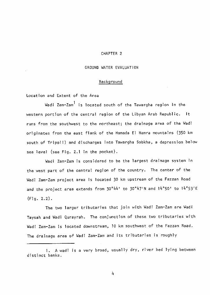
Wadi Zam-Zam 1 is located south of the Tawargha region in the

western portion of the central region of the Libyan Arab Republic. It

runs from the southwest to the northeast; the drainage area of the Wadi

originates from the east flank of the Hamada El Hamra mountains (350 km

south of Tripoli) and discharges into Tawargha Sobkha, a depression below

sea level (see Fig. 2.1 in the pocket).

Wadi Zam-Zam is considered to be the largest drainage system in

the west part of the central region of the country. The center of the

Wadi Zam-Zam project area is located 30 km upstream of the Fazzan Road

and the project area extends from 30 0 44' to 30 ° 47'N and 14 0 50' to 14 ° 53 1 E

(Fig. 2.2).

The two larger tributaries that join with Wadi Zam-Zam are Wadi

Taysah and Wadi Qurayrah. The conjunction of these two tributaries with

Wadi Zam-Zam is located downstream, 10 km southwest of the Fazzan Road.

The drainage area of Wadi Zam-Zam and its tributaries is roughly

1. A wadi is a very broad, usually dry, river bed lying betweendistinct banks.

5

u.)

17)

oTr

I..m

E_v0

_ _c co._ (..) ô &•.)a • o u a,

.....a. " a

a o 018

co — 512 -alita ...v Ti — 0o = u > , 0

Z: 0 w > 6-..- ,_c

•-c) 0

Lu-J< ino

•

"7:/7:5 o Jo (i) .

3 2 t °23 Pa.13, 3 cpcn E.Zr- 12, E 2 ("5 -F- D

• f .fi g:

.o

/

_,

-1

I• ,

I . ,----,,--,--- -----, ._____ii--

- ------------- --t --. .

. t• ____________•

a J . . AllialiP---N------N•hh.--wiahwrg1

—

111•411nnn••

a.,., .•21 0

.tri4 4

f I.

' 6oLncq-

.„ ---. - - _ _ ----- - - -41 I, AftI,

liçflir'' 14 cr)4 ,

•.' t:ii>-a

%4 :'. 2 F.'.1 1•••• ' 1

V% ES 114» fii..:4\ •Zr b ,...: ,0

t ""r....111111110.1 ,0

0 i::, t'ASt4, 2‘ ki s ';,':

9 .‘‘,!F',..,

..:44; 1.,•,:,

•

,....

•n•t, V

Tr

2

6

rectangular with an area of approximately 4,000 km2

(Fig. 2.2). The

approximate length of the main stream is 70 km.

An agricultural project extending along the Wadi main stream was

started in 1572 and is operated by the Libyan Ministry of Agriculture and

supervised by the Libyan Army.

Climate

The climate in the Wadi Zam-Zam region is similar to most warm

desert climates. It is extremely hot in summer with a drastic change in

temperature between day and night. The average daily temperature is 38°C

(the maximum temperature occurs in June; 44 ° C) and it drops to an average

low in December of 4 °C (Fig. 2.3). The mean annual precipitation is

roughly 52 mm. Rainfall occurs infrequently with random distribution and

as shower activities, and is negligible during the summer season. Within

15 years of recorded rainfall, there were only two significant storms

that caused some runoff into the Wadi and its tributaries. The mean

annual precipitation distribution is shown in Fig. 2.4. The rainy season

normally begins during the second half of October and continues with few

scattered showers until April. December and February have the highest

rainfall.

Hot winds with high velocities are common phenomena in the Wadi

Zam-Zam region. These winds act effectively in transporting sand. Sand-

storms are well-known in the area; sand and dust are lifted and conveyed

by wind in sufficient volume to blacken the sky at times. This wind is

locally known as Kibli and it blows from the south. The wind is a very

ODL._ (t)= t—

=7:I- 17.1

is.-o) a)O. a.E E11)

12EE= =E E74 ._C c2 2

oo

0

o0

o_(r)

J .M 1 c

0cr)

Z a)

z0 cc

D 2 Ero—D NJ1EcorJ

I

-0

I J

CL

<:t

J I

CO•INn U-1

11.n

(1)

•• nn

I IO LO 0 in 0 tO 0 1.0 0 to rf1

LO cr re) II) C‘.1

(00) 38r11V83dIAlaL

7

1-c.)o

I I I I I I

o o Lc) o oro rr) N N

W W ) 11\7.d NIVJ cr)

8

u-)

owl

L)

o

o

9

active factor, causing high evaporation and transportation of sand,

forming sand dunes of different sizes and shapes.

The relative humidity is very low in summer, not exceeding 20

percent. Fog frequently occurs in the early morning with high density,

but disappears a few hours after sunrise. In the winter, cold winds

usually blow from the north with an average speed of 15 km/hr, resulting

in an average daily relative humidity of about 44 percent.

Topography

Topographically, the Wadi area consists chiefly of sand dunes

with gentle slopes generated by wind, and surrounded by a broad desert.

Downstream, the banks of the Wadi slope steeply. Alluvial fans cut the

banks here and there with increasing frequency downstream. Generally,

the profile of the Wadi from upstream to downstream slopes gently, with

an average slope along the valley bed of 2 m/km. The maximum elevation

is about 250 m (msl) upstream and the lowest elevation is -4 m (msl) at

the mouth of the Wadi (Fig. 2.2).

Natural Resources and Population

Earlier, agricultural activity in the area was entirely dependent

on the occasional rainfall during the fall and winter seasons. Unless

there was rainfall, the land was barren except for small scattered shrubs

and shallow-rooted plants (Fig. 2.5). These plants were considered the

main food source for the regional animals. Hand-dug wells, scattered

along the Wadi, with an average depth of 25 meters, were used for

domestic supply and animal watering. These wells are limited in yield

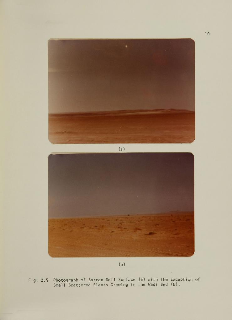
( b)

Fig. 2.5 Photograph of Barren Soil Surface (a) with the Exception ofSmall Scattered Plants Growing in the Wadi Bed (6).

10

11

to less than 1.5 m3/hr and yield water of poor quality. When flooding

occurred (about once every 10 years), the Wadi bed was seeded to grains,

such as wheat and barley, and the edges of the hills were used for

raising the animals.

The chief towns in the project area are Bogran and Kedahia, which

are downstream with small populations of less than 1500 each. The major

occupation of the people in the two cities is business. Bogran serves as

a commercial service station on the road between Tripoli and Benghazi,

which are the major cities in Libya. Bogran also provides some govern-

mental employment. Kedahia serves as a commercial station also, on the

Fazzan Road. Residents of these two towns did own the land in the Wadi

Zam-Zam and its vicinity, but it is now controlled by the government.

Also, some nomads come to the area after the rainy season.

In late 1972, the agricultural project was initiated, dependent

on deeper ground water in the area. The primary purpose was to settle

the nomads and to provide them with a more stable food and water supply.

The plan allots 25 ha to a family and fruits are the principal crops to

be grown.

Surface soil in the Wadi, which averages 1/2 km in width, is

alluvial and appears homogeneous with only small variations in grain

size. The surface soil is underlain by subsoil which is normally com-

pacted and cemented with lime in some places. Upstream, the surface

soil has been eroded away and subsoil appears on the surface. Shallow,

rocky soils occur in a few small, isolated areas and near the mountains.

12

The only sizable water resource available in the area is ground

water. Since 1972, hydrological investigations have been carried out in

an attempt to develop the ground water and thirteen deep wells (1,000 m)

have been drilled along the valley (Fig. 2.6). All of these wells tap an

artesian aquifer and have an average yield of about 50 1/sec and an

average static pressure of about 6.5 atm (65 m above the land surface).

At present, 1,400 ha are reclaimed and are being planted with selected

varieties of olive trees, almond trees, and table grapes. The process of

development is continuous and there are plans now to develop a total of

3,500 ha and to drill eight additional deep wells.

At present, the main problem is the ground water temperature

which averages 56 °c. In addition, there is not enough information on the

aquifer that is already under development concerning recharge, discharge,

areal extent, leakage, etc.

Previous Investigation

This report is based not only on the published information, but

also on unpublished works and personal knowledge of the area and personal

interpretation of the available data and information that were obtained

in the field by the author.

To date there has been no detailed study carried out on the area.

Most of the previous studies were regional, referring very briefly to the

project area. Jones (1964) briefly described the ground water hydrology

in the Tawargha area and Hungraben, referring briefly to the ground water

in the Zam-Zam area. Gaudrazi (1972) reported on the surface geology of

the central part of Libya and described very briefly the surface geology

1 3

14

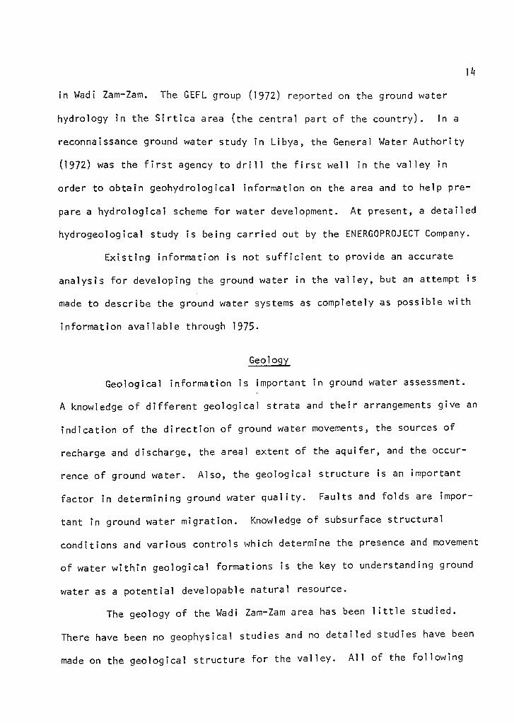
in Wadi Zam-Zam. The GEFL group (1972) reported on the ground water

hydrology in the Sirtica area (the central part of the country). In a

reconnaissance ground water study in Libya, the General Water Authority

(1972) was the first agency to drill the first well in the valley in

order to obtain geohydrological information on the area and to help pre-

pare a hydrological scheme for water development. At present, a detailed

hydrogeological study is being carried out by the ENERGOPROJECT Company.

Existing information is not sufficient to provide an accurate

analysts for developing the ground water in the valley, but an attempt is

made to describe the ground water systems as completely as possible with

information available through 1975.

Geology

Geological information is important in ground water assessment.

A knowledge of different geological strata and their arrangements give an

indication of the direction of ground water movements, the sources of

recharge and discharge, the areal extent of the aquifer, and the occur-

rence of ground water. Also, the geological structure is an important

factor in determining ground water quality. Faults and folds are impor-

tant in ground water migration. Knowledge of subsurface structural

conditions and various controls which determine the presence and movement

of water within geological formations is the key to understanding ground

water as a potential developable natural resource.

The geology of the Wadi Zam-Zam area has been little studied.

There have been no geophysical studies and no detailed studies have been

made on the geological structure for the valley. All of the following

15

interpretations are based on well-log information for the wells along the

Wadi and on surface observations. Information from well logs for wells

ZZ1 and ZZ2 is shown graphically in Fig. 2.7. Figures 2.8a and 2.8b,

showing geological sections of the middle and upstream of the Wadi,

respectively, were prepared by the author with the help of the

ENERGOPROJECT staff.

Quaternary

Alluvial deposits of Quaternary age form the land surface along

the Wadi. The alluvial formation was deposited either by wind or water,

or by a combination of both. The thickness of the alluvial layer changes

from place to place, ranging from zero upstream (40 km from Fazzan Road)

to 30 m downstream. The alluvial material consists of sand and silt

uncemented at the surface to about 2 m and cemented with lime below that

level.

Eocene

Sedimentary rocks of Eocene age, locally known as the Jabel Wadan

formation, underlie the alluvial deposits and form the structure of the

drainage area of Wadi Zam-Zam and its tributaries. They consist of

chalky limestone which is locally known as the Zamam formation. Also,

these formations include the Bir Zidan formation, which is mainly shelly

limestone and marl or many limestone. This formation outcrops upstream,

forming low permeable layers. Some scattered volcanic rocks are down-

stream where there are extrusive volcanic rocks, chiefly basalt and

olivine, mostly from the Tertiary age (see Fig. 2.9).

msomm

WARM

10km

NMI=IMINMEN

1101111211113C11311131Cli1111111111nosrisin1311:1111131

SCALE

9

Dolomite

Marl

Fine Sandstone

Limestone

Clay Limestone

Chalky Limestone

100

O

— 100

—200

—300

—400

- T500

—600

—700

—800

—900

AINT08 81

16

Fig. 2.7 Hydrogeological Cross-Section along Wadi Zam-Zam.

•

17

Vertical Scale 1500

_44111/

135N 30° 46

• E 14° 50' 15"

ROUGA CHALK/AMAMINEMMIN,MI NM.1111/411111n

011111WVIAL=MOMI I II WA I FA I 1 I I MiT

VANNIMMIAMMIAn?...:

AMINIEVANIONMAREI=IMMOMMEMM

75

Waal Chalky limestone vlNIA Dolomitic limestone Slope debris

(a) Middlestream

Fig. 2.8 Geological Cross-Section.

4/1111111/411111111•1.AIINVAIIIIII

411111•1111/4111111

N 30 0 40' 30"E 14° 54' 16"

Vertical Scale 1:100

Chalky limestone

Dolomitic limestone

Slope debris

1112•111111A

%WA; 0 -

° 0 0 •cr, • •• • • •

18

160

155

(h) Upstream

Fig. 2.8, Continued.

1 9

20

The elevation of the bottom of the Eocene formation, referred to

mean sea level (msl), ranges from -100 m upstream to -50 m at ZZ2 down-

stream. The thickness of the formation ranges from 200 m at well ZZ1 to

80 m at well ZZ2 (Fig. 2.7) and averages 150 m.

Paleocene

The Paleocene formation of the Tertiary age is not present at the

surface in any part of the Wadi. This formation, under the Eocene forma-

tion, consists of marl, shell, and marly limestone which is locally

fossiliferous. The upper part of the formation includes the Zamam forma-

tion which is of late Cretaceous age. The formation deepens approxi-

mately 1.5 m/km toward the northwest (see Fig. 2.7). The top of the

formation is -100 m (msl) at ZZ1 and -50 m (msl) at ZZ2, with an average

thickness of 110 m.

Cretaceous

Mizda Formation. The Mizda formation of the upper Cretaceous age

lies under the Paleocene formation. It consists of alternating layers of

chalkly limestone, marl, and clay limestone. It appears in all well pro-

files along the Wadi at an average depth of -300 m (msl) (Fig. 2.7) and

has roughly a constant thickness of 170 m. This formation is charac-

terized by a low potential water yield of less than 10 m3/hr. Mizda

limestone is locally fractured, which makes it difficult to penetrate by

rotary drill because of a loss of circulation problem.

Tigrina Formation. The Tigrina formation of the upper Cretaceous

age was penetrated by all the drilled wells in the area to a depth

21

ranging from -450 m (msl) at ZZ1 to -390 m (msl) at ZZ2. The Tigrina

formation consists of marl, many limestone, clay limestone, small local

layers of sandstone, limestone, and dolomite (see Fig. 2.7). South of

the Wadi Zam-Zam area, the Tigrina formation contains an aquifer of

moderate potential yield. This formation could have a high potential

where it is intercepted by faults.

Yefrin and Gharian Formations. Yefrin and Gharian lime was pene-

trated by most of the deep wells drilled in the west and central part of

the country. These formations consist chiefly of chalky limestone and

clay limestone with locally dolomitic limestone and manly limestone. The

average thickness of these formations in Wadi Zam-Zam is about 170 m

(GEFL, 1972). The Yefrin-Gharian formation of the lower Cretaceous for-

mation outcrops at Jabel Nefusa, 300 km west of the valley and is a

source of many springs in that region. This formation is intercepted by

a series of faults in many places and by intensity fractures crossing the

formation which produce a moderate aquifer potential yield.

Chicla Sandstone. Chicla sandstone is the upper part of the con-

tinental series which belongs to the lower Cretaceous and upper Paleozoic

ages and extends over 50 percent of Libya. This series of sandstones is

known as Nubian sandstone. The formation was penetrated by deep wells in

the Wadi at depths from -800 m to -850 m (msl) (see Fig. 2.7). The

average thickness of the formation is about 80 m without significant

changes along the Wadi. It is chiefly sand and silt, generally weakly

cemented, and intercepted locally by thin layers of clay and marl. There

22

is no significant information on the lateral extension of the formation

in Wadi Zam-Zam. This formation is a high potential artesian aquifer.

Ground Water

As mentioned earlier, surface water in Wadi Zam-Zam is essen-

tially negligible. Therefore, the ground water that has accumulated over

a period of centuries is the most important water resource in the area.

Ground water in Wadi Zam-Zam area is either fossilized water or comes

from regional aquifers that do not receive local recharge.

Aquifers

Four different aquifers have been identified during the recon-

naissance phase. The water in these aquifers varies in quality and

quantity. The deepest (fourth) aquifer is the most important one for

developing in Wadi Zam-Zam. The other three aquifers will be discussed

only briefly.

First Aquifer. The first aquifer is alluvial and the deeper

chalkly limestone and calcarenites of Eocene age. The fill probably

belongs to the Tertiary period and is very heterogeneous. The depth to

the water table varies from 30 m to 120 m below the surface.

The thickness of the first aquifer is approximately 100-150 m.

There is no available information concerning the water stored in this

reservoir. The water contains 3,000-3,500 ppm of total dissolved solids.

The aquifer is locally recharged by occasional rainfall which is

usually very small. Numerous dug wells tapping this reservoir along the

Wadi were used for livestock watering and domestic supply. Camels were

2 3

used to withdraw water from these wells at small rates which do not

exceed 1.5 m 3/hr.

Generally, this aquifer provides low yields and water of poor

quality. However, when broken by numerous faults crossing Wadi Zam-Zam,

this aquifer may have good hydraulic characteristics. At present, there

is no information available on the hydraulic parameters of this aquifer.

Second Aquifer. The second aquifer is made of dolomitic lime-

stone, calcarenite, and chalky limestone belonging to the Mizda forma-

tion. It reaches to -200 m (msl) at ZZ2 upstream and -270 m at ZZ1

(see Fig. 2.7). Its thickness is approximately 160 m.

The second aquifer is separated from the first one by very thick,

continuous layers of dark marl approximately 200 m thick. The water in

this aquifer occurs under artesian conditions. The water level in the

wells stands close to land surface (+4 m at ZZ2 and -12 m at ZZ1).

The hydraulic characteristics of this aquifer seem to be poor

according to short tests conducted at ZZ2. The total dissolved solids

content is approximately 3,300 ppm. The water temperature is

approximately 40 ° C.

Third Aquifer. The third aquifer is made of chalky limestone and

dolomitic limestone belonging to the Gharian formation. The top of the

aquifer is about -650 m (msl) at ZZ1 and -580 m (msl) at ZZ2 (see

Fig. 2.7). Its thickness is approximately 80 m. The water in this

aquifer occurs under artesian conditions. The aquifer is overlain by

confined layers made of marl, marly limestone, and clay limestone with an

24

average thickness of 180 m. The water level in the wells stands at 50 m

above land surface.

There is no information available on well yield from this

aquifer, but the hydraulic parameters of the aquifer seem to be good, as

was shown by a short test conducted at ZZ2. The water quality of this

aquifer seems to be relatively good (TDS = 1,300 ppm) and the water

temperature is roughly 54 ° C. A detailed study will be carried out to

determine the possibility of developing this aquifer with others for

agricultural purposes.

Fourth Aquifer. The fourth aquifer is mainly Chicla formation

with dolomitic limestone at the top belonging to the Aintobi formation.

The top of the formation is roughly at -800 m (msl). The thickness of

the aquifer is approximately 200-250 m. The water in this aquifer occurs

under artesian conditions and the potentiometric surface in all wells

tapped from this aquifer stands at an average of 65 m above land surface.

A confining bed overlies the aquifer made of clayey limestone, marl, and

many limestone intercepted by thin layers of hard dolomites belonging to

the Yefrin formation of an average thickness of 120 m. This aquifer is

described in greater detail in the next section.

Characterization of Chicla Sandstone Aquifer

Extent of the Aquifer

The aquifer is the upper part of the continental series belonging

to the lower Cretaceous and the upper Paleozoic periods and extends over

more than 50 percent of Libya. This series is usually called Nubian

25

sandstone, which is also well-developed in Algeria, Egypt, and the Sudan.

This aquifer is considered the most important one when dealing with water

recources of Wadi Zam-Zam.

Discharge and Movement

Discharge from the aquifer in Wadi Zam-Zam is increasing every

year by the increased number of wells tapping the aquifer. There is no

obvious natural discharge from the aquifer in the study area or its

vicinity. Thirteen wells have been drilled along the Wadi and eight more

wells will be drilled according to present plans. The General Water

Authority has estimated the volume of water from each well to be 50 1/sec

(180 m3/hr). The project plans call for the development of 3,500 ha.

The amount of irrigation water required per hectare is estimated at

9,000 m 3/ha/yr. This leads to the total amount of water required of

31.5 x 106

m3/yr. The General Water Authority estimated that the maximum

discharge from the Chicla sandstone aquifer should be 20 x 106

m3/yr.

A rough estimation of the hydraulic gradient along the Wadi is

5 x 10-4

towards the northeast. Therefore, the natural flow was esti-

mated to be 1.8 x 10-1

1/sec-m2 of front, which is negligible by assuming

an average thickness of 100 m and a transmissivity of 1.8 x 10-2

m2/sec.

Nevertheless, if new information showed this value to be underestimated,

it would only increase the water resources available. Consequently, the

main part of the water available from the deep aquifer in the Wadi will

come from storage.

26

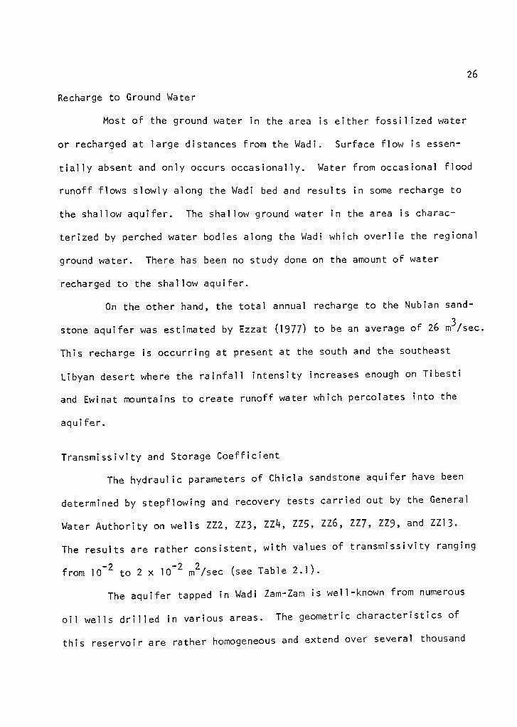
Recharge to Ground Water

Most of the ground water in the area is either fossilized water

or recharged at large distances from the Wadi. Surface flow is essen-

tially absent and only occurs occasionally. Water from occasional flood

runoff flows slowly along the Wadi bed and results in some recharge to

the shallow aquifer. The shallow ground water in the area is charac-

terized by perched water bodies along the Wadi which overlie the regional

ground water. There has been no study done on the amount of water

recharged to the shallow aquifer.

On the other hand, the total annual recharge to the Nubian sand-

stone aquifer was estimated by Ezzat (1977) to be an average of 26 m3/sec.

This recharge is occurring at present at the south and the southeast

Libyan desert where the rainfall intensity increases enough on Tibesti

and Ewinat mountains to create runoff water which percolates into the

aquifer.

Transmissivity and Storage Coefficient

The hydraulic parameters of Chicla sandstone aquifer have been

determined by stepflowing and recovery tests carried out by the General

Water Authority on wells ZZ2, ZZ3, ZZ4, ZZ5, ZZ6, ZZ7, ZZ9, and ZZ13.

The results are rather consistent, with values of transmissivity ranging

from 10-2 to 2 x 10-2 m2/sec (see Table 2.1).

The aquifer tapped in Wadi Zam-Zam is well-known from numerous

oil wells drilled in various areas. The geometric characteristics of

this reservoir are rather homogeneous and extend over several thousand

2 7

Table 2.1 Hydraulic Parameter of Chicla Sandstone Aquifer asDetermined by Step-Flow Test.

Well Date ofNo. Operation

ZZ1 June 1973

ZZ2 March 1973

ZZ3 January 1975

ZZ4 January 1975

ZZ5 February 1975

ZZ6 February 1975

ZZ7 June 1975

zz8 June 1975

ZZ9 July 1975

zzio August 1975

ZZ11 June 1975

ZZ12 September 1975

ZZ13 March 1975

Average

Transmissivity

(m2/sec)

EstimatedAverageDischarge

Storage RateCoefficient (1/sec)

1.2 x 10-230

1.55 x 10-2 4o

1.88 x 10- 2

2 x 10 -4* 60

2.1 x 10 -270

2.2 x 10 -2 60

1.26 x 60

1.44 x 10 -2 4o

1.8 x 10 - 250

.85 x 10-2 30

.88 x 10-250

2.3 x 10-2

6 0

1.6 x 10- 2

6 0

1.88 x 10- 2 30

1.88 x 10-2

*The storage coefficient was only determined with ZZ4 flowing and

ZZ3 as an observation well.

28

square kilometers. Therefore, there is no reason to imagine important

changes in behavior of this aquifer except over longer periods of time.

The cone of depression for ZZ8 after 48 hours of flow is shown

in Fig. 2.10. The piezometric decline was determined by measuring the

pressure decline at ZZ7, ZZ12, and ZZ4 while ZZ8 was flowing and cal-

culating the line of equal piezometric head decline assuming a homo-

geneous aquifer.

The values of transmissivity and storage coefficient that will be

used for calculating the effect of well discharge on the piezometric head

are as follows: T = 1.8 x 10-2

m2/sec and S = 2 x 10

-4 .

As no lateral boundary is expected to affect the long-term

behavior of the aquifer, results using these parameters can be considered

as minimum values and would increase with the contribution from the over-

or underlying strata, which can occur after a certain period of time.

Interference Effect within the Well Field

The size, shape, and the growth rate of the cone of depression

resulting from discharge are essentially determined by the transmissivity

and storage coefficient. The rate of discharge is affected by the depth

of the cone of depression. The coefficient of transmissivity is propor-

tional to the thickness of the aquifer.

In order not to depend on the yield of each well for drawdown,

the interference of different wells has been calculated in terms of

specific drawdown, DiQe . The specific drawdown is the drawdown per unit

of discharge and does not depend on Q. The specific drawdown is

2 9

30

calculated on the basis of an assumed 100 percent well efficiency using

Theis' equation (Theis, 1935):

1.9D/Q = W(u)e T

1.87 r 2 S u —

Tt

(2.1 )

(2.2)

where

D = drawdown, m;

Qe = well discharge, m3/hr;

T = transmissivity, m 2/day;

W(u) = well function of u;

r = well radius, m;

S = storage coefficient; and

t = time, days;

Figure 2.11 shows the relation between specific drawdown and

distance for the considered 5 days, 10 years, and 50 years. Knowing the

distance between the wells, information from Fig. 2.11 is then used to

calculate the specific drawdown induced by all the wells: 1) in the

middle of the well field (Table 2.2); and 2) on one extremity of the well

field (Table 2.3).

Piezometric Head

As a result of continuous flow from drilled wells, the pressure

in the artesian aquifer decreases and that reduces the discharge from the

0 0 0CD CnJ

09S/ 1-1-1/ 11•190/ 0 NMOON1V0 01.d103ciS

31

Table 2.2 Specific Drawdown in the Middle of the WellField (ZZ8) Induced by 13 Wells.

InterferingWell

Distanceto ZZ8(m)

Specific Drawdownin ZZ8

(m/m 3/sec)

ZZ1 17,400 24

ZZ2 12,400 26.7

zz3 10,600 28

zz4 8, 000 30.5

zz5 15,900 24.5

ZZ5 14,000 25.5

ZZ7 3,100 39

ZZ8 1 110.5

ZZ9 3,600 37.5

zzto 7,40 0 31

zzti 16,10 0 24.5

ZZ12 10,700 28

ZZ13 19,600 22.5

4Total 52.2

32

Table 2.3 Specific Drawdown, D/Qe , Induced by 13 Wellsin the Extremity of the Well Field.

InterferingWell

Distanceto ZZ13

(m)

Specific Drawdownin ZZ13

(m/m 3 /sec)

zzi 4,400 35.6

ZZ2 31,000 19

ZZ3 9,600 29

ZZ4 12,100 27

ZZ5 8,700 30

ZZ6 6,700 32

ZZ7 16,700 24.2

ZZ8 19,600 22.5

ZZ9 23,100 21.5

ZZIO 26,600 20

ZZ11 34,900 17.8

ZZ12 28,500 19.5

ZZ13 1 110.5

Total 408.6

33

34

aquifer. The measured piezometric level of Chicla sandstone expressed in

mean sea level for 1974 is shown in Fig. 2.12. Taking into consideration

the well field including the wells planned in the near future (ZZ14,

ZZ15, ZZ16, ZZ17, ZZ18, ZZ19, and ZZ20) and assuming the values of the

hydraulic parameters (T, S) that were obtained from the flow test

(T = 1.8 x 10 -2 m2/sec and S = 2 x 10 -4 ), it is possible to calculate the

effect after 5 days, 10 years, and 50 years. it is assumed for the cal-

culation that each well will flow at an average continuous yield of

50 1/sec; therefore, the piezometric level decline in the Chicla aquifer

will be calculated using Fig. 2.11. On the other hand, the analysis of

the step-flow test data concludes that the piezometric decline produced

by the flowing well can be expressed as a function of the discharge:

D = 500 Qe (2.3)

where D is the water level decline (in meters), and Qe is the discharge

(in m3/sec). The drawdown induced by all wells at ZZ4 is shown in

Table 2.4 for the three time periods.

The drawdowns after 10 years of exploitation (Fig. 2.13), ranging

from 17.3 to 19.0 m, are still acceptable. Nevertheless, it has to be

noted that specific capacity, and consequently the artesian yield, of the

wells would decrease in the future not only because of the normal water

level decline, but also because of the increase of friction losses inside

the wells due to corrosion of the pipe.

There have been no continuous measurements made of drawdown for

existing wells except measurements were taken on ZZ4 after one year and

Cr)

LI.

35

Table 2.4 Estimated Drawdown Induced by Each Well in the ChiclaSandstone Aquifer for Well ZZ4.

Drawdown Drawdown Drawdown

Distance after 5 days after 10 yrs. after 50 yrs.

(in) (m) (n) (m)

o 4.o6 4. 0 5 4.05

too 1.85 3.5 3.85

200 1.6 3.19 3.78

300 1.4 3. 0 3.4

400 1.3 2.89 3.29

500 1.2 2.79 3.14

600 1.15 2.70 3.1

700 1.1 2.62 3.01

800 1.05 2.585 2.25

1,000 .95 2.49 2.85

1,400 .835 2.3 2.7

I,800 .735 2.2 2.6

2,000 .695 2.15 2.55

3,000 .50 1.995 2.38

4,000 .40 1.85 2.24

5, 000 .33 1.75 2.13

6, 000 .285 1.685 2.05

7,000 .2 1.6 1.99

8, 000 .185 1.55 1.9

9, 000 .11 1.5 1.88

10,00 0 .1 1.45 1.8

20,000 . 08 1.15 1.5

30,00 0 . 06 .95 1.3

36

ce1

-Cs

C7)

37

IJ

38

4 months with four wells operating. The drawdown for that well was 6 m,

which is close to a calculated value of 5.6 m. The true value was prob-

ably a little higher because the time of recovery was very short.

Well Specifications

Artesian Head and Discharge

Thirteen wells already have been drilled and tapped from the

Chicla formation. All of these wells are artesian with pressures at the

surface ranging from 55 to 70 m (static). The average pressure is 65 m

above the ground surface.

From the flow-test data analysis, which is shown in Fig. 2.14,

the following equation was derived to express the relation between the

pressure and the yield:

P = 65 - 100 Qe - 4,500 Qe2(2.4)

where P is the piezometric head above the surface (in meters), and Qe is

the well discharge (in m 3/sec).

Therefore, the problem is to fix Q such that the corresponding

pressure at the head of the well is equal to the sum of the following

terms:

1. The pressure, Po

required for operation of the irrigation system

(P0 = 15 m).

2. The water level decline in order to keep the yield constant for

10 years (D).

oco

Cc

H0 wCr

Z

0_ wo u-

O wct rt

ctu-i

(f)—

L Li 0crio_3

coo

ui) ONISVO JO dal.]H.1. 9N18è:GA]è:i LIFISSL1c:1 112M co.

u-

39

1+ 0

3. The interference from the nearby Wadis which are located at the

west of the area and are expected to be developed soon (I ). This

interference is assumed to be 10 m.

Hence:

P = Po + D + I

( 2.5 )

where D is expressed by equation (2.3). Therefore:

P = 15 + 500 Qe + 10 (2.6)

Then, the combination of equations (2.4) and (2.6) gives:

900 Q2 = 120 Q - 8 = 0 (2.7)

This equation has only one positive solution:

Q = .05 m3/sec

Therefore, in order to keep enough artesian pressure to maintain a con-

stant well discharge for the next 10 years, the well discharge should

not exceed 180 m3/hr.

Well Spacing

Under artesian conditions, water released from storage is

entirely due to the compressibility of the aquifer material and that of

the water. Therefore, the losses in hydraulic head caused by the flow

from each well will propagate very fast. In addition, the hydraulic con-

ductivity of the aquifer is fairly high (10 m/day). Then the depression

41

cone induced by discharging will be wide and flat. As a result of these

two factors, the drawdown induced by each well will cover a great

distance.

When wells are spaced close together, their cones of depression

may overlap and additional drawdown results. The wells should be placed

at desirable distances to reduce the overlapping between wells as much as

possible to keep high well efficiency. Well spacing involves hydraulic

factors as well as economic factors. Cost of pipe installation and

maintenance of the pipe system will increase in the space between wells.

The optimum space was determined by Theis' equation for deter-

mining the optimum well spacing in a simple case of two wells pumping at

the same rate (Campbell and Lehr, 1973):

r = 9.09 x 105 CQe2

MT(2 .8)

where

r = optimum well spacing,

C = cost of operation (pipe and auxiliaries),

Qe = flow rate (m3/min),

M = capital cost (drilling and construction of the well), and

T = transmissivity (m2/day).

It is assumed for the calculation that the well flow is 3 m3/min

and the capital and operations costs were 105 and 6.6 x 10

4 Libyan

pounds, respectively.

42

Therefore, the desirable space between wells is recommended to be

3.5 km. This space could produce 1.9 m drawdown in the discharging well

due to the neighboring wells, after ten years of continuous discharge.

Well Design

Well design for water production involves selecting the proper

dimensions for the diameter and depth of the well and the proper

materials to be used. Proper design aimed at protecting the well assures

long life and good performance.

Cost and hydraulic characteristics are the two main factors that

control well design; these two factors should be analyzed properly and

accurately. The hydraulic factor is involved when designing the well for

highest production and efficiency in terms of specific capacity. The

cost factor includes the cost for drilling, materials, installation, and

cost of operations, maintenance, and replacement.

A large well diameter will increase well efficiency and probably

increase the yield. But, as the well diameter increases, the cost will

increase too. Therefore, cost and technical factors must be properly

analyzed.

Under artesian conditions, well structure consists of two

elements. One is the casing which serves as a conduit through which the

flow occurs from the aquifer to the land surface. The other is the

screen or the intake portion of the well where the water enters from the

water-bearing formation to the well.

Under natural flow from an artesian aquifer, the main factors

that control well construction are head losses produced inside the well

43

which control the pressure at the surface and the cost. The pressure at

the top of the aquifer is proportional to the head loss. Therefore, the

diameter of both the casing and the screen must be large enough to assure

good hydraulic efficiency for the well.

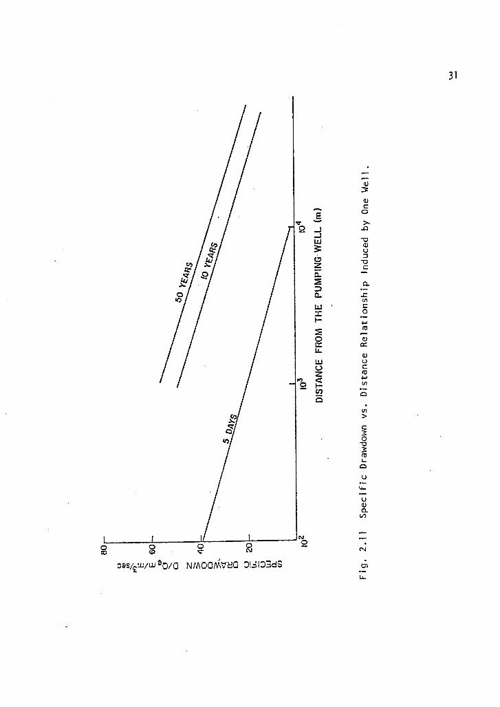
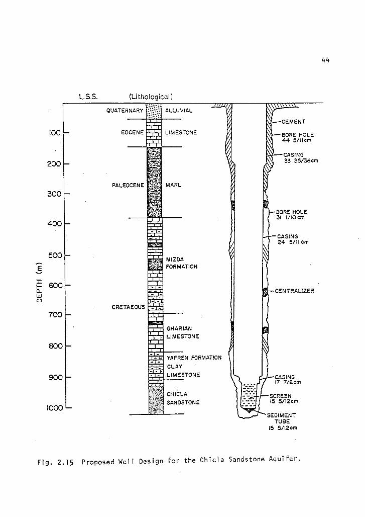
In Wadi Zam-Zam, the well yield is estimated as 50 1/sec (180

m3/hr). Based on Johnson Division's (1972) criteria and drilling sample

analysis by the General Water Authority, coupled with the author's

experience, the following program is recommended for well design in the

Wadi (Fig. 2.15):

1. Installation and cementation of 45.5 cm conductor tube down to

approximately 20 m.

2. Drilling with 44.5 cm diameter down to 250 m.

3. Setting down and total cementation of a 34 cm casing (H40).

4. Drilling with 31.1 cm diameter down to 1,000 m.

5. Geophysical logging, consisting of a conventional electrical log

only.

6. Setting down and total cementation of a 24.5 cm casing (H40 or

J55) from 34 cm casing shoe down to the top of the water-bearing

formation.

7. Setting down of screens, stainless steel, bridge slotted slot 60

(15 mm), 15.4 cm diameter, 6 mm wall thickness as a minimum.

8. Developing for 48 hours, or as needed.

9. Flow test for 72 hours minimum.

44

L.S.S. (Lithological)

100

200

QUATERNARY : . ALLUVIAL

41

111

EOCENE

--aINMEN=-MOUM— LIMESTONE=NM

PALEOCENE MARL•%

300

=NM

400 =1•111•111•11E111•2

moms

500MIZDAFORMATION

1— 600

=CB

CRETAEOUS

700

GHAR1AN

LIMESTONE

800 /,MMUM

111:311. YAFREN FORMATIONammo CLAY

900 LIMESTONE=MUMN-

CH I 'CLA

SANDSTONE1000 —

CEMENT

BORE HOLE44 5/11 cm

CASING33 35/36cm

BORE HOLE31 1/10 cm

CASING24 5/11 cm

CENTRALIZER

CASING17 7/8cm

SCREEN15 5/12 cm

SEDIMENTTUBE

15 5/12 cm

Fig. 2.15 Proposed Well Design for the Chicla Sandstone Aquifer.

45

Estimating Head losses Inside the Well

The average yield of the wells in Chicla sandstone aquifer is

50 1/sec. The friction losses corresponding to this yield will range

from 8 to 13 m according to the well. This friction loss was determined

from the manual provided by the manufacturer of the screen and casing and

distributed as follows:

34 cm casing 1 m

24.5 cm casing 5-8 m

15.4 cm screen 2-4 m

The only way to decrease the friction loss would be to use a larger

diameter of casing and screen. Unfortunately, this would double the

cost of the well while the capacity still is limited to 50 1/sec in order

to keep the artesian yield nearly constant for at least 10 years.

Water Quality for the Chicle Sandstone Aquifer

Chemical Analysis

Since all wells tap the same aquifer, chemical analyses were

carried out by the author for eight selected wells. Immediate analysis

was done in the field using Hach and conductivity meter to obtain depend-

able results because the composition of the sample may change before

arriving in the laboratory. The results are shown in Table 2.5.

Certain chemical analyses were also made in the laboratory from

samples collected from the same wells. The results of these analyses are

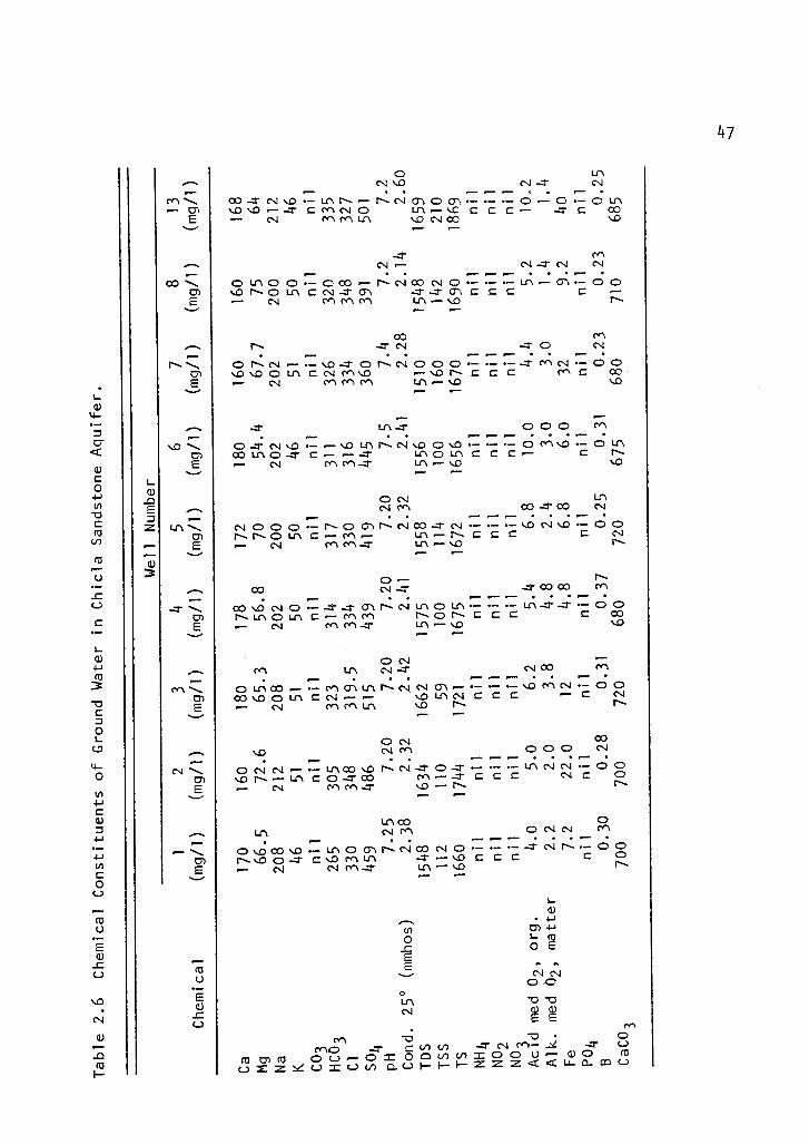
shown in Table 2.6. They indicate that the water quality for the aquifer

Table 2.5 Field Analysis of Ground Water in Chicla Sandstone.

WellTemp.(°C) pH

Cond.(25°C)

HCO3

(mg/1)

Total CO2

(mg/1)

02

(mg/1)

H2

S

(mg/ 1 )

ZZ2 55 7.4 2.32 353 75.9 nil .59

ZZ4 57 6.9 2.42 384 73.0 nil .76

ZZ5 57 7.2 2.52 353 68.9 nil .59

ZZ6 56 6.6 2.49 390 92.9 nil .85

ZZ7 55 6.6 2.28 335 86.0 nil .76

ZZ8 55 7.3 2.14 360 82.8 nil .85

ZZ13 56 6.3 2.60 366 70.9 nil .96

ZZ1 55 7.2 2.38 335 83.9 nil 1.09

Average 56 7.1 2.39 359 79.3 nil 0.81

1+6

47

0 ln

CNI NO (NJ --1" CNJ••n a • •••n .•

CO •••T C...4 %.,0 ... LI\ r•••• .-- 1"-n N C71 0 0-`, .- 0 .-- 0 .- 0 In‘.0 N.0 .-- -1- C C•r") Cs4 0 LrN ,- ..c c c c - -1- c co.-- CNI re\ CY1 In N.0 CNI CO NO

fr1

CNJ CNI CNI CNI

. . • • • •Lnoc).-coo— N. C-4 CO 04 Q Lr% cr,•-ooN. Q 1..r\ C c.1 -4- a\ --1- 0-1 C C C C

- N Ce1 CYN N.•••nn .,nnn

CO enN. -I' N -1" 0 CV

• .••• 0 • ••n ..•n •nn • • pm.. •

o r-, c...i — .- .0 --/- o r-, c-4 o o o .- ..- -1- C'n Cs/ .- 0 0

..0 ,..0 o ix\ c cs, ren .0 — .0 N. C C C 0'1 C CO.-- CNI rel M M in .- NO N.0

gI•MP

.11•••, 1•••

1.1"1 0 CD 0, CY\• • • . •

0 --T N-O Lfl CNI NC) 0 s.0 v.') ‘.0 0 Inco id, o L.r.\ (=> C C C C r•-••

CNJ L/1 N.0 NO

CN1 Lr\

CNI C11 CO --T CO C•4• • 1n• •n• .n•• • • • •••••

N 0 0 0 N. 0 CT% N. N CO 4- '.0C) Lf1 C 1.11 P- N. C C C C

••n- CNI V\ CY\ -.1"11•n• 1••••

P- N-CO CO CO Cn

••n• • • 1n•••• e•`n •••. • • • I•••• •

CO NO CNI --T CT% CV LC\ 0 In Lr‘ -.T 0

N. Lc% cD i.r c: m m N. Q N. c: c: C c: CO0.4 M Lrn .0 %ID

.1,••nn

• Nr,r1 LI-N CV - Cs4 CO ffl

• • I•••• • • 1•••• •

0 LC\ CO re\ CT\ Ls% r-, C CNI CT\ -- .0 0

CO ‘.0 0 C cs) ..01.4"\NCCC C

Cs.1 re1 LIN NO N.

• N CO

NO C'1 C\ 0 0 0 C•4

• • •-• • • • .

CNI CNI •- In CO NO 0 0

N.0 C Q --T CO 0,1 C C C C

Cs.) 4-11 NO r•-n- ..••••

LI\ CO 0

Ln N ce% 0 C'NI C•4 m• 1•••• • • Im•• •n• 1...• • • • •••• •

0 S..0 CO '.0 • ln 0 C71 N. CV CO Cs4 0 .- •- -1" CNI N. .- 00

1"-••• N.0 CD -...T C N.0 rel tn -1" ,-- NO C C C C 0

.--• CNI CNI rel -.1- Ln ,--- NO N.,•••

cf*,

csrl•

cr20

C (r)

O (...) 0 2 0 0 cr) V) 2 0 CD I-) •-• CI.) Q a:1

= cr.) rm. L) I— < < m

•n•••

CC)

is relatively uniform. The small variation could be related to the

inter-bedded shale layers, or experimental error.

The chemical analysis of the ground water indicates that the

water is acceptable for irrigation usage (Israelsen and Hansen, 1962)

The electrical conductivity is slightly high. The total hardness ranges

from 675 to 720 mg/1, which is very high, or approximately 50 percent of

total dissolved solids.

Corrosion Tendency

Well water of Wadi Zam-Zam was studied to determine the corrosi-

vity of the water for pipes used as well casing. Metallic corrosion

occurs when a metal reacts with its environment, whether it is a solid,

gaseous, or aqueous liquid. Water corrosion takes place when some fac-

tors are favorable. As a principle, the corrosion constituents of

natural water are: a low pH and dissolved gases (oxygen, carbon dioxide,

and hydrogen sulfide), acidity, alkalinity, a high salinity, a high

stability index, and a low saturation index (Zarazzer, 1975). All these

determinations were studied to determine possible corrosion of the

installed casing.

The ground water of Wadi Zam-Zam is free from oxygen. This

element is usually a dominant factor in corrosion when it is present in

water.

The amount of free carbon dioxide found in the water ranged

between 68.9 and 92.8 mg/l. This amount is itself not a factor of corro-

sion by water containing or saturated with dissolved oxygen. The CO2

content reacts like an acid by increasing the acidity of water.In our

49

case, the measured pH in the field is between 6.3 and 7.25. A pH of

6.0 to 8.0 will increase the CO2 content of water, but has practically no

effect on corrosion rate, especially when the water is free of oxygen.

The main effect of dissolved carbon dioxide seems to be its influence on

the solubility of calcium and magnesium carbonate.

Acidity accelerates corrosion. The chief characteristic of iron

corrosion in acid water is that it proceeds with the evolution of a con-

siderable amount of hydrogen without the formation of an insoluble

coating. At pH 5.5 and lower, a rapid hydrogen gas evolution starts and

corrosion is accelerated. This condition does not occur in Wadi Zam-Zam

water.

Hydrogen sulfide is produced by sulfate reduction. Its amount is

very low -- 0.59 to 1.09 mg/1 expressed as H2S. In the laboratory, water

was tested qualitatively by lead acetate paper and a smell was noted.

However, this test is not precise at low concentrations. Hydrogen sul-

fide dissolved in water acts as an acid and produces corrosion on iron,

forming iron sulfide and hydrogen. This corrosion can be accelerated by

the presence of free oxygen. This condition is not present in the

ground water.

Both carbon dioxide and hydrogen sulfide act as an acid in water.

It means that the pH of water should be very low. A pH between 6.3 and

7.25 is not a low pH, because it is a common pH of natural water. The

effect of corrosion of these two gases is too small to cause a serious

corrosion on casing pipes. On the other hand, if this ground water con-

tains free dissolved oxygen, corrosion of casing may be more serious.

50

Table 2.7 shows the corrosion effects in casing by other indices.

As indicated, all samples had a low Fe ion concentration, indicating

little corrosive activity. Additional interpretation of the data is

given as follows.

Table 2.7 Corrosion Effects on Casing in Deep Closed Wells.

Well No.Saturation

IndexStability

IndexTotal Iron

(mg/1)

1 -0.05 7.3 7.2

2 -0.3 8.0 22.0

4 -o.3 7.5 4.8

5 - 0 . 0 5 7.2 6.8

7 -o.8 8.2 32.0

8 -0.2 7.8 9.2

13 -0.9 8.1 40.0

Saturation Index. The saturation index indicates the degree of

instability with respect to calcium carbonate deposits. A positive value

indicates the tendency for calcium carbonate deposits. A "zero" satura-

tion index denotes that the water is exactly at equilibrium with respect

to calcium carbonate. All ground water samples have a negative index

value; that is, there is no tendency for calcium carbonate deposition.

Stability Index. The stability index indicates a quantitative

measure of calcium carbonate scale formation. In this case, all values

are positive:

51

1. A value less than 6.0 or 6.0 indicates scale formation.

2. A value between 6.0 and 7.0 indicates an equilibrium.

3. A value between 7.0 and 8.0 indicates no protective coating of

calcium carbonate.

4. A value higher than 8.0 indicates corrosion.

Ground waters are on an average between 7.1 and 7.8 for flowing

wells which means very low corrosion. For wells not flowing, the

stability index is higher than 8.0. This type of corrosion is static

corrosion resulting from long contact of water/casing (see Table 2.8).

Table 2.8 Corrosion Index Analysis in Wadi Zam-Zam Deep Flowing

Wells.

Well Number

4 6 5 7 8 2 1 13

Fe (mg/1) 4.8 6.0 6.8 7.2 9.2 22.0 32 40

SaturationIndex 3.0 -0.7 -0.05 -0.05 -0.2 -0.3 -0.8 -0.9

StabilityIndex 7.5 7.1 7.0 7.3 7.0 8.0 8.2 8.1

-

In the report written by Branko and Brikish (1974): 1) the water

is corrosive because of H 2S and CO 2

content; and 2) the well will be

obsolete in 5 years.

These arguments cannot be taken into consideration. Corrosive

gases, marble test, and pH do not indicate an excessive corrosion suffi-

cient to limit the age of a well to 5 years.It is too difficult to make

52

a prognostication for the working life of wells; nobody can say if their

life is limited for 15 or for 30 years.

The appearance of red water is not necessarily a measure of the

degree of corrosion, but from the static condition of the well this

appearance can be greater or smaller depending on the static time of the

well water/casing contact.

All ground waters contain variable amounts of iron, and iron is

abundant in the earth's crust and may be in the Chicla formation. It

means that the presence of this element in water flowing normally, as in

wells ZZ1, ZZ3, ZZ4, ZZ5, and ZZ6, may arise from two sources: ground

water and/or casing. In order to identify the source of this iron, it is

necessary to determine the iron content in different levels of Chicla

formation.

Conclusions and Recommendations of

Ground Water Evaluation

The field data were not enough to make an accurate assessment.

There is no information available on the other three reservoirs that

could help to evaluate the ground water system in the valley. Most of

the pumping test data were recorded in the flowing wells and there are

not many records of any observation wells. The maximum flowing test

duration was five days.

However, in the light of the data available from the field and

the data being calculated, the following assessments can be made:

1. The results of the primary test conducted by the General Water

Authority (1973) indicate a similarity in temperature, pressure

53

head, and total dissolved solids between the Gharian limestone

formation and the Chicla sandstone aquifer. This indicates

strongly that there is a possibility of a hydraulic connection

between the two aquifers.

2. The variation in transmissivity along the valley is mainly

related to the variation in the thickness of the aquifer and the

impurities (marl, clay, dolomite, limestone) that intercept

locally Chicla sandstone (Fig. 2.7).

3. The spatial change in the transmissivity is related to the change

in pressure head. The lower the transmissivity, the higher the

formation losses and, consequently, the lower the pressure head.

4. The pressure head gradient is sloping toward the northeast with

an approximate value of 5 x 10-5 and the flow is estimated to be

1.8 1/sec-m2 toward the northeast.

5. The calculated drawdown after ten years of operation shows that

there will be extensive drawdown in the center of the valley.

This is essentially because of small spacing between wells (well

interference).

6. Water level decline in water wells during the flowing test showed

roughly a steady-state condition a few hours after the flow

started. This is mainly a result of the large areal extent of

the water-bearing formation and the high uniformity of aquifer

parameters.

In order to evaluate ground water resources in the valley and to

make the best interpretation, more field data are needed, especially in

54

the other aquifer parameters, and water level measurement in the differ-

ent wells.

The conservation of the water resources and the proper use of

this expensive and limited commodity make it necessary to adopt a

hydraulic scheme which takes into consideration:

I. The specific characteristics of each well (pressure and artesian

yield).

2. The total yearly water production which must not exceed 20 x 106

3m which can be exploited from 13 wells.

3. The high temperature of the water.

4 • The possible additional resources from the shallow aquifers

during the period of peak requirements.

5. The actual distribution of soils, and consequently the crops,

which will determine the best irrigation system.

At present, the hydraulic system in use in the project makes any

control of water production and water use impossible. Thus, it is urgent

to reorganize the water management properly.

The proper amount of water from the Chicla formation is estimated

as 20 x 10 6 m3 ; the annual water resource which can be exploited from 13

wells which are already drilled (50 1/sec). This amount of water will

provide irrigation water for 2,500 hectares. Up to this point, it is

recommended that no more wells should be drilled in the same aquifer.

ln order to guarantee a constant artesian yield for each well and

the pressure required for irrigation for the next 10 years, the following

recommendations could be taken into consideration:

55

1. The total number of wells has to be limited to 13 (50 1/sec).

2. Distance between wells must be 3.5 km as an average.

3. The total discharge of the 13 wells should be limited to 20 x 106

m3/year.

L. The average yield of each well should be limited to 50 1/sec.

Considering the actual area that the Wadi Zam-Zam project plans

to plant and the water requirements of certain periods of the year, as in

summer, consideration should be given to develop other aquifers to pro-

vide additional water.

First Aquifer

The characteristics of the first aquifer are not known at

present. A program of necessary geophysical surveying should be per-

formed to investigate the first 200 m. At the same time, the project or

any other agency could undertake the drilling of some shallow wells to

check the water quality and the capacity of this reservoir, even though

it is not expected to have high capacity.

Second Aquifer

At present, the development of the second aquifer is not recom-

mended for both the bad quality of the water and for the poor hydraulic

characteristics of the formation. However, it is important to drill two

or three wells in order to check these two factors.

56

Third Aquifer

If the same hydraulic parameters of Chicla sandstone aquifer are

assumed for the third aquifer of Gharian chalky limestone, an additional

well could be proposed to tap this aquifer in order to supply additional

water (250 1/sec).

There is no detailed study being made concerning the Gharian

chalky limestone in relation to Chicla sandstone, but initial results

indicate a hydraulic connection between the two aquifers. The tempera-

ture of the water is roughly the same as the fourth aquifer (55 ° C) and

the chemical properties are also similar -- approximately 1,300 ppm for

TDS. Therefore, before any development of ground water from the third

aquifer, it is necessary that this relation should be studied very

carefully.

This evaluation of the water resources has to be a primary con-

sideration and it should be reviewed as soon as possible according to the

present condition in the Wadi. The following data should be collected:

I. The quantity of water extracted each month or year (by reading

the water meter installed on each well).

2. The water level in each well should be measured each month.

These measurements should be made after the well has been closed

for a few days so the steady-state condition may be observed.

3. The water level in the well during pumping and a measurement of

rate of discharge of the well at the same time.

57

This proposed program of ground water development could provide

the agricultural project with 900 1/sec (28 x 10 6 m 3/year) for a first

approximation.

Since the water requirements are much higher during summer, the

following solutions are recommended to meet the requirements during the

whole year:

1. The deep artesian well will flow at the same rate during the

whole year supplying approximately 650 1/sec continuously to meet

the water requirements during the winter.

2. During the summer, wells from other aquifers (Gharian and

alluvial) supply additional amounts of water required. This

solution will have two advantages:

a. Shallow water will cool down the hot water from the artesian

aquifer.

b. Fresh water coming from the artesian aquifer will reduce the

brackish water from the shallow aquifer.

CHAPTER 3

GROUND WATER COOLING

Introduction

As mentioned in Chapter 2 of this report, the ground water

temperature averages 56 ° C (Table 2.5). For irrigation purposes, this

temperature is detrimental to crop production. The Zam-Zam project

authority has no specific cooling policy. Sometimes the irrigation water

flows from the well to a water tank cooled to near ambient temperature,

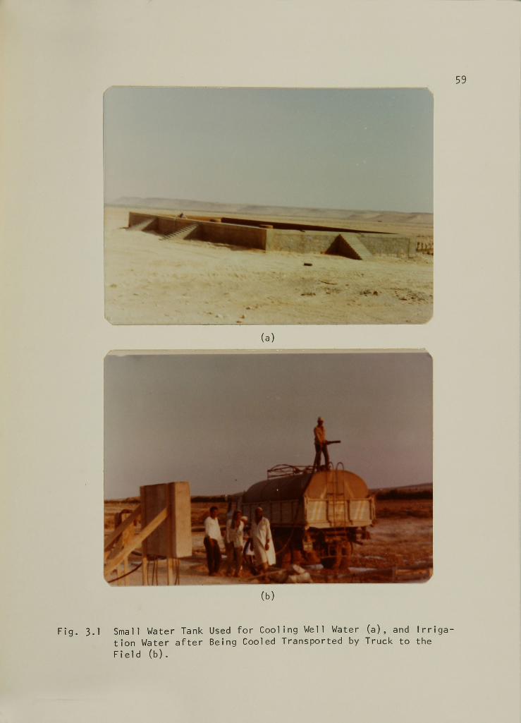
then the water is transported by tank truck to the field (Fig. 3.1).

Sometimes they use water directly from the well without cooling for irri-

gation so the applied water has an extreme temperature. Another way they

use for cooling the irrigation water is for the irrigation water to flow

through long (1/2 km) ditches where the water temperature is lowered by

5-10 °C (Fig. 3.2). These methods are not satisfactory for technical or

economic reasons.

The construction cost of the small cooling tanks (150 m3 ) is an

average of $2,000 each. The time needed for cooling the irrigation water

in tanks to an acceptable temperature averages 48 hours. In addition,

the method of water transportation by tank trucks from the cooling tanks

to the field is entirely uneconomical and impractical.

in the area of well ZZ3, where the water was used directly, the

measured temperature of the water near the crop was 48 ° C when the

ambient temperature was 28°C. This temperature is too extreme for most

58

59

(b)

Fig. 3.1 Small Water Tank Used for Cooling Well Water (a), and Irriga-tion Water after Being Cooled Transported by Truck to theField (b).

6 0

Fig. 3.2 Water Flowing through Long Ditches for Cooling the Irrigation

Water.

61

crops. Using water tanks for cooling purposes is not economical and is

ineffective. Flowing of irrigation water through ditches causes high

water losses through seepage and evaporation, without adequate cooling.

There are no established guidelines for maximum irrigation water

temperature, but high temperature in the root zone may reduce plant

growth, and modify the soil by increasing the rate of chemical reaction

between the soil compounds and chemical constitution of the soil water

(Zarazzer, 1975). Since soil temperature affects seedling emergence,

growth rate and time of maturity, these three factors affect directly

crop production.

In this part of the study, results of an investigation of cooling

methods that have been used frequently in cooling of water in power

plants will be represented. The three methods are cooling ponds, spray

ponds, and cooling towers. The study will examine these methods economi-

cally and with respect to water consumption.

Evaporative Cooling -- Heat Dissipation

Evaporative cooling is cooling of liquid (water) by three

combined energy transport processes which physically differ. The three

processes are:

1. Latent heat or heat of evaporation, heat transfer by mass diffu-

sion and convection (4)e

)

2. Sensible heat transfer, through contact by conduction and

convection ((pc).

62

3. Heat transfer by radiation, which is important only in cooling

ponds or open reservoirs. In other types of cooling systems,

heat transfer by radiation may be neglected.

Energy flux due to evaporation plays a major role in the total

heat dissipation from a water surface. It is a function of the vapor

pressure gradient regardless of the temperature difference at the air-

water interface and goes mainly to the atmosphere. In contrast, heat

transfer through contact depends on the temperature difference between

the water (Ts ) and the air (T

a) and flows either to or from the water

body.

Both processes are related and affect each other. The combined

effect of the heat ((p c) and mass transfer ((p a ) on the water surface heat

exchange is shown in Fig. 3.3 for different conditions. When Ts > Ta ,

the heat flux from the water body, (p n , equals the sum of both processes:

'r (1) c (1) e

As a result, the water surface temperature continues to fall. When

Ts < Ta , the heat flux from the water surface becomes:

4)n = 4)e - 4) c

As the temperature of the water surface continues to fall, it increases

the cpc

and decreases the (I)e. Dynamic equilibrium is reached when cp

c = 'e

and the net energy flux from the water's surface equals zero, or:

T > TT5 a

63

On 1 COe CPc

T = E

Fig. 3.3 Heat Flow in Evaporative Cooling as a Result of CombinedEffects of Heat and Mass Transfer. -- From Berman (1961).

Ts =E

(see Appendix A for definition of symbols) which is the hypothetical

point at which heat flow from the water body equals heat flow to the

water surface.

Cooling Pond

A cooling pond is defined as an open water body whose function is

to dissipate unwanted heat from a thermal source as well as the natural

heat input. A cooling pond receives hot water from one end and dis-

charges cooled water from the other end.

A cooling pond is most acceptable for evaporative cooling in

regions where land is inexpensive. Compared with other cooling systems,

i.e., towers, cooling ponds require a larger area of water surface for

heat dissipation to reduce water temperatures to desirable limits.

A cooling pond has the advantage of Tow maintenance and pumping

costs. However, it has higher water consumption than other systems and

its design is sensitive to site conditions (Scofield and Fazzolare,

1971). Cooling pond design depends on accurate calculation of the heat

flux dissipated from the water surface to the atmosphere. A small error

in prediction of heat flux may lead to a large pond surface area which

may reject the cooling pond as an economical heat dissipator.

Detention time is determined by the design. In a good design,

detention time should be less than twenty-four hours; some designs may

require several days detention time.

65

In this study, the time frame to be used is long enough for

monthly meteorological parameters to be adequate to predict the heat flux

and evaporation rate from the water surface. A completely mixed pond is

assumed for analysis.

Completely Mixed Pond Energy Budget

A completely mixed cooling pond (no vertical water temperature

gradient) may be approximated because of the pond design, wind, turbulent

flow, instantaneous differences in vertical temperature, and water flow

rate.

The significant components of the energy balance for a pond

completely mixed are shown in Fig. 3.4. The water surface receives

energy by:

1. Short-wave solar radiation.

2. Atmospheric long-wave radiation.

3. Waste thermal discharge.

The water surface dissipates energy by:

1. Long-wave back radiation.

2. Mass transfer (evaporation) or latent heat.

3. Sensible heat, or convection and conduction.

4. Seepage from the bottom and sides of the pond. This term can be

usually neglected because it is small compared to the other

terms.

Many studies have been carried out on the process of heat

exchange between water surface and the atmosphere. The process can be

Long WaveAtmospheric

- Radiation

Short Wave SolarYs Radiation

Back Radiationcl)b

Heat Load from

1. P Thermal Resource

Other Energy

14)P1) Input

30-

(t) a bRadiation

ReflectedAtmospheric

(sbSolar Energy

Reflected

66

Fig. 3.4 Heat Exchange Mechanism at the Pond Surface. -- From Hogan,

• Ltepins, and Reed (1970).

67

identified and evaluated fairly accurately. One of the earliest discus-

sions on the concept of heat dissipation from a pond was presented by

Cummings and Richardson (1927). Lima (1936) developed a set of empirical

curves to determine the overall heat transfer coefficient. These curves

were used to predict the mean pond temperature (without the effect of the

longitudinal or vertical temperature gradient). Lima was one of the

first to compare actual pond temperatures with those predicted.

Throne (1951) developed empirical curves by using an empirical

technique based on the energy budget in natural water bodies (no thermal

load) and equilibrium temperature measurements. LeBosquet (1946) pre-

sented an analytical technique to determine the cooling capacity of

natural ponds. This technique was expanded by Langhaar (1953). Langhaar's

empirical technique is based on the energy balance of natural water. It

takes into account the effect of the vertical and longitudinal tempera-

ture gradients. Langhaar's work was modified by Velz and Cannon (1960)

for a water body receiving thermal waste discharge. Data used were col-

lected from Shreveport, Louisiana, and rivers in Michigan.

The most comprehensive work on energy budgets appeared in the

Lake Hafner study as reported by Anderson (1952). Ediger and Geyer

(1965) and Brady, Grave, and Geyer (1969) presented a comprehensive study

of the energy balance technique. They provided charts and tables for

most cases of the heat dissipation process for different water bodies

(lakes, rivers, well-mixed, steady, unsteady, etc.).

The mass balance equation for a cooling pond at dynamic equilib-

rium condition can be expressed as (Hogan et al., 1970):

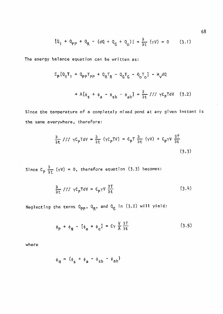
68

a[Q I + QPP QR (dQ TQ G Q0 )] = E- (Yv) = 0 (3.1)

The energy balance equation can be written as:

CP[Q I T ! + QPPTPP + QRTR - Q G

TG

- QoTo]HvdQ

A4 s (1) .9 (1) sb 4)ab ] = Ti- fff yC pTdV (3.2)

Since the temperature of a completely mixed pond at any given instant is

the same everywhere, therefore:

a DT7.--t Iff yC

apTdV = (yCpTV) = CT Tt- (y11) + C pyV

(3.3)

9Since C — (11/) = 0, therefore equation (3.3) becomes:

P Dt

DIff yC pTdV = C yV 31.

P Dt

Neglecting the terms Qpp, QR , and QG in (3.2) will yield:

V DT(I) - E(l'e (I) c ]

= CIp N

(3.4)

(3.5 )

where

4) N = (4's (I)a - 4) 56 4)ab )

69

and

(PID = (fi 7

Each term of equation (3.5) will be discussed separately.

According to Stefani's law, all bodies radiate energy by electro-

magnetic waves and do so at a rate proportional to the fourth power of

their absolute temperature. The wavelength of the radiation is given by

Wien's law:

Xm

= C I IT

where T is the absolute temperature of the body radiation energy, and C I

is a constant. Therefore, the hotter the body, the shorter the wave-

length and vice versa.

Short-Wave Solar Radiation

The magnitude of solar radiation is a function of the time of

day, altitude, season, and cloud cover. It can be calculated with undue

difficulty. Marciano and Harbeck (1954) evaluated two empirical formulas

that could be used to compute cp s as functions of the sun's altitude and

cloud cover. Kennedy's equation (Marciano and Harbeck, 1954) evaluated

solar radiation of a clear sky at the exterior of the earth's atmosphere

and the length of the actual path of solar beams to the path through the

Zenith ratio. As a result of the complexity that is involved in

computing solar radiation transmitted to the surface, it is easier to

measure it. A pyranometer is the instrument commonly used. Solar radia-

tion can be estimated from charts (Hogan et al., 1970).

70

Atmospheric Long-Wave Radiation

In contrast to solar radiation, atmospheric long-wave radiation

is easier to calculate than to measure. Several empirical equations have

been developed (Hutchinson, 1957; Koberg, 1963). Brunt's formula as

described by Koberg (1963) has been used extensively for evaluating

atmospheric radiation:

(1) .a = 4.4 x 10 - 8 (Ta + 273.15) 4 [C B + .031(P) 112 ] (3.6)

The value of CB can be determined from the air temperature and

the ratio of measured solar radiation at the surface to clear sky solar

radiation (Brady et al., 1969). Atmospheric radiation also can be

measured directly at night by the Gier-Dunkle flat plate radiometer or by

the Thornthwaite net radiometer.

Reflected Atmospheric Radiation, (p ab

The reflected atmospheric, long-wave radiation energy by the

water's surface can be estimated by the reflectivity coefficient (R s):

Rs

=ab

hpa (3.6a)

and is relatively constant at .03 as reported by Hutchinson (1957).

Therefore, the reflected atmospheric radiation by the water's surface may

be taken as:

7 1

l'ab = . 03 (l'a W/m

2(3.60

where W (watt) = 14.34 cal/min.

Reflected Solar Radiation, (1-I'sb

As for reflected atmospheric radiation, the reflectivity coeffi-

cient 4sb/(1)s) of the water surface to solar radiation can be used to

determine reflected solar radiation. The reflectivity ratio is a func-

tion of solar altitude and the amount and type of clouds. Empirical

curves which show the reflectivity ratio as a function of the above were

developed in the Lake Hafner study.

At particular sites, there is no need to measure all four terms.

It is more convenient to measure a combination of these terms by

Cummings' Radiation Integrator which gives the net absorbed radiation:

(1) NI = ci a + (1's - 4)ab - sb W/m

2

(3.6c)

Bear in mind that neither solar radiation nor atmospheric radiation

depend on water surface temperature.

Back Radiation 6, Tbr

The rate of heat emitted by back radiation from the water surface

can be calculated from Stefan-Boltzman's law:

br = ea(T

s + 273.15)

4

(3.7 )

cpbr

= 5'5 x 10

-8(T5 + 273

•15)

4W/m

2

(3.7a)

72

which gives a good prediction, usually within 85% accuracy (Marciano and

Harbeck, 1954).

In contrast to other radiation terms, energy flux by back radia-

tion is constant on both clear and cloudy nights.

Energy Flux Due to Evaporation, cpe

In view of the fact that evaporation plays an important part in

heat transfer from the pond surface, it is very important to make an

optimum estimation of evaporation rate. There are two terms that deter-

mine the energy flux resulting from evaporation: specific flux per kilo-

gram of water leaving the air-water interface, and the rate of mass

transfer at the air-water interface.

Many empirical methods to estimate evaporation have been

developed. Most of them are derived by using the theories of momentum

and mass transfer. The most notable analytical work is that of Sverdrup

(1937-38). The most comprehensive study on water budget was undertaken

at Lake Hefner (Marciano and Harbeck, 1954). Meyer (as reported by

Linsley, Kohler, and Paulhus, 1958), as well as Koberg, Harbeck, and

Hughs (1959) for Lake Colorado, have also developed important equations.

In addition to those already mentioned, similar equations have been

developed by many others.

Most experimental data for large bodies of water are limited to

the natural body where the difference between the surface water tempera-

ture and the equilibrium water temperature is very small. Limited work

has been undertaken on water bodies receiving waste thermal discharge

where the temperature differences are great. Therefore, most empirical

73

equations used for natural water bodies cannot be applied to provide an

accurate prediction of evaporation rate where heated effluent is being

discharged.

Vapor movement from an evaporative surface is a combination of

two forces, free convection bouyancy force and forcrd convection (wind

action). Most of the derived empirical formulas have underestimated

evaporation by neglecting the free convection force. Therefore, most of

these equations performed poorly when tested in the Lake Hafner study.

A simple expression found for estimating the rate of evaporation

was given for artificially heated water by Meyer (as reported by Velz and

Cannon, 1960), as well as Koberg et al. (1959) for Lake Colorado, who

have also developed important equations:

4)e = f(w2 )(P s - P a )

(3.8 )

The equation expresses evaporation as a function of vapor pressure dif-

ference times a wind function. Wind function has been subjected to many

field studies. It can be expressed as a function (Brady, 1970):

f(w2 ) = a l a 2w2 a 3w2 2

(3.8a)

The Meyer equation performed satisfactorily for Lake Hafner and Lake

Eucombeen in Australia.

For artificially heated ponds, Brady et al. (1969) estimated the

wind function value from field data from lakes in Texas and Louisiana:

74

f(w2) = a 4. bw 22 (3.8b)

Equation (3.8) can be expressed as a function of temperature

instead of pressure difference (Brady et al., 1969):

(1)e = Ww)(T s - Td ) (3.9)

where

= (P s - Pa )/(T s - Td )

Convection, (1)c

Energy flux by convection from water to air is a function of the

temperature gradient near the air-water interface. It is similar to the

energy flux by evaporation. Bowen (1926) is among the first to derive an

expressed ratio between energy flux by convection and evaporation using

the diffusion theory:

(I) T Ta p

= = .00k76 sR

(Ps - Pa )q5e 7-65-(3.10)

(Pc = d'eYe

By substituting (3.10) into (3.11):

= B'f(w)(T s - Td )

(3.11)

(3.12)

75

where B' is the Bowen ratio which is approximated as .47 (mm Hg/ ° C);

therefore:

(P c = .47(T s Ta )f(w) W/m2 (3.12a)

Methods of Calculation

The computation procedure of various cooling pond design param-

eters begins with computing the design and equilibrium temperature from

the ambient meteorological data. The heat exchange coefficient (the time

rate exchangeable heat per unit area per unit temperature gradient) and

the pond area are then computed for each specific criterion. The surface

water temperature is then computed. With the pond area known, the

average monthly evaporation rate is then determined.

Substituting equations (3.7a), (3.9), and (3.12) into equation

(3.5) gives the general energy balance equation for completely mixed

ponds:

r V 9T= A P NI

306 - 4.48 T s - .025 Ts 2'PY 3t '

- S(Ts

- Td)f(w) - .47(T

s - T

a)f(w) W/m

2

(3.13)

At dynamic equilibrium conditions, (3.13) can be written for isolated

water bodies as:

76

0 = (1) N - 306 - 4.48 E - .025 E 2 - $E(E - Td )f(w)

- .47(E - Ta)f(w) wim2 (3. 1 4)

The rate of heat transfer in natural ponds (no thermal water

input) can be expressed as (Brady, 1965):

dln K(E - T

n)/yC

Ph (3.15)

dt -

which can be written as:

4 = AK(E - Ts ) (3.16)

Under dynamic conditions, equation (3.16) is similar to equation (3.5).

Substituting (3.16) into (3.13) yields:

(Pp4 = ---+ K(E - T)

As (3. 1 7 )

The heat exchange coefficient, K, can be derived by subtracting

(3.14) from (3.13) after substituting (3.17) into (3.13) and assuming

= :

(Pp

E4) = + 4.48(E - T s ) + .025(E2

- T 2

)

+ + .47)(E - T s )f(w) W/m2 (3.18)

77

The cooling demand can be expressed by Newton's law:

(I)p = KA(Ts - E)

(3.19)

Subtracting (3.17) from (3.18) gives (Brady et al., 1969):

K = 4.48 + 0.025(E + T s ) + + .47)f(w)

w_m-2_ 0c -1

(3.20)

The second term of (3.20) can be neglected (Brady et al., 1969) and the

heat exchange coefficient can be expressed as:

K = 4.48 + (a 4. .47)f(w) (3.21)

The wind function has been determined from field observations

(Brady et al., 1969) as:

f(w) = 9.2 + .46 w2 W/m2-mm Hg

(3.22)

The value of $ is defined as the pertinent slope of the chord

between the points representing T s and Td on the saturated vapor pressure

curve providing there is exact convergency and not approximation (Brady

et al., 1969):

a 0.35 + .015 Tm + .00012 Tm2 mm Hg/°C

where

Tm

= (Td + E)/2

78

Therefore, the equilibrium temperature can be computed from the ambient

meteorological data by using (3.14) for solving E and defining the heat

exchange coefficient K in (3.21) as the equilibrium exchange coefficient

(KE) yielding (Scofield and Fazzolare, 1971):

E = - KE +KE2 - .4N - 306 + (Td + •47Ta )f(w)]

(3.23)

The pond area required to dissipate heat can be determined

explicitly. Rearranging equation (3.16) for temperature distribution in

a recirculating flow-through completely mixed pond gives:

KA = Q In [(Td - E)/(Ts - E)] (3.24)

The equilibrium temperature and the heat exchange coefficient are

coupled. Both depend on water temperature and meteorological conditions.

Therefore, an iterative technique can be used to avoid the solution of

quadratic expressions in equation (3.16).

The exchange coefficient is computed by using (3.20) in terms of

T s, when Ts

and the value of a are known. The area of the pond is then

computed using equation (3.24). This method provides accuracy and

simplification as the value of Ts differs from one case to another. The

combination of equations (3.24) and (3.19) results in the surface

temperature expression:

Ts=E+Q /Q In [(T 1

- E)/(Ts - E)]

(3 .2 5)

79

Knowing the pond surface area, the operating surface temperature

necessary to dissipate the cooling demand is then computed by equations

(3.20) and (3.25). An iteration technique is used to avoid the solution

of the quadratic expression for the two values of the effective surface

temperature and heat exchange coefficient.

The total heat of evaporation rate is computed by multiplying

equation (3.9) by the surface area:

(pc = af(w)(T s - Td )A (3.26)

Therefore, the evaporation rate can be computed by dividing equation

(3.24) by the heat of evaporation (H) :

Qe = 1235[Bf(w)(T s - Ta )A/Hv ] kg/hr (3.27)

where

Hv = 597.3 + .56(Ts

- 32.2) kcal/kg

A computer program developed to accomplish the calculation is listed in

Appendix B.

Results and Discussion

Climatological data from 1925 to 1970 were obtained from the

Libyan Weather Bureau for the city of Hon. The difference between the

climatological data of Hon and Wadi Zam-Zam was considered negligible.

These data were analyzed to determine annual, monthly, and summer (June,

July, August, September) statistical parameters; results are shown in

80

Table 3.1. Final pond design criteria were set for an average summer to

consider peak water demands. Computation of average monthly parameters

is based on well discharge temperatures ranging from 48.8 to 60 °C. Con-

sideration is given for a water temperature lowering (AT) of 16.7 to

22.2 °C. A constant well discharge of 50 1/sec was used and a completely

mixed pond was assumed.

The computed equilibrium temperatures compared with the approach

(difference between pond discharge temperature and water equilibrium

temperature) are shown in Fig. 3.5. As weather data were studied,

monthly variation in dry-bulb temperatures became apparent. Summer

months exhibit the highest dry-bulb and equilibrium temperatures. This

results in the lowest sensible heat transfer from the water surface for

any given cooling demand.

For well discharge temperatures of 48.9 to 50 ° C and AT = 22.2 ° C,

the summer dry-bulb temperature exceeds that of pond discharge tempera-

ture and the approach reaches its minimum. Under the conditions con-

sidered, heat flow from the atmosphere to the water surface through con-

tact is counteracted by latent heat which becomes the major process of

cooling the water body.

As illustrated in Fig. 3.6, the required area for a given cooling

demand decreases exponentially, with increase in well water temperature.

Additional cooling demands necessitate larger areas. It is clear that

surface area is affected by a combination of the approach and the well

discharge temperature. Sensible heat flux is considered the major factor

in this relationship. Because of higher equilibrium and dry-bulb

81

Table 3.1 The Statistical Results of 45 Years of Climatological Records.

Month

Temperature ( ° C) RelativeHumidity

(%)

Radiation(4/m2 )

WindVelocity(m/sec)

Dry-Bulb

Wet-Bulb

DewPoint

January 11.1 6.3 2.5 47.00 324.7 4.3

February 13.0 6.8 2.8 41. 00 377.9 5.3

March 16.1 8.6 4.2 33. 00 429.5 5.3

April 20.7 11.1 6.4 28.00 482.1 6.4

May 23.9 13.3 8.3 27.00 536.6 6.4

June 28.3 15.0 10-9 24.00 568.7 6.4

July 27.8 15.6 12.2 26.00 565.8 7.4

August 27.8 15.6 11.7 26.00 542.8 6.4

September 27.2 16.1 12.9 31.00 504.3 6.4

October 21.7 15.0 11.3 35.00 424.5 5.3

November 16.7 10.6 7.7 43. 00 359.5 4.3

December 12.2 15.0 2.2 35.00 323.0 4.3

AnnualAverage

22.2 12.8 7.2 35.00 476.9 5.7

Summer 27.8 15.6 12.2 25.00 564.6 6.7Average

o.

I ill// /

/

1// // / d//•1/

/.7/ 0//

///////

///

Ltl

82

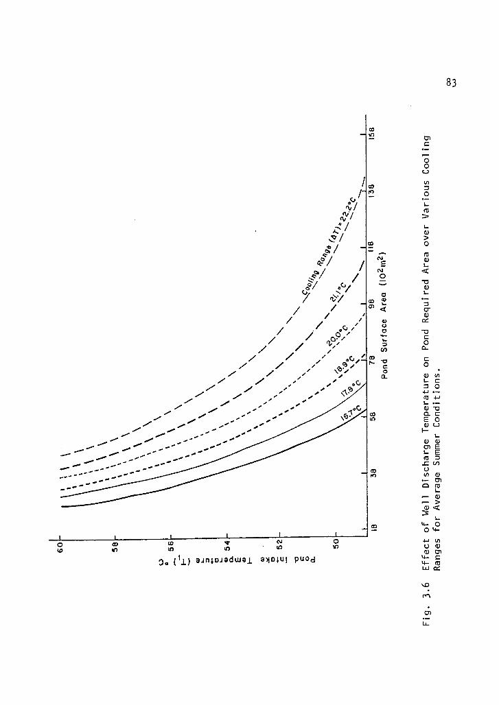
oco

0

ncs

83

oo1.0 cr;

00

c—)

0

• , - co c/ ./. / ,..9 / r- -cs

c 0.." ..i.

o.• 0 c, a. a) (1)

L. C

.../ ..". • /.•

/.. .01 .• ' .• d. ..1 es m o....- .../

v.. 4-,

.....",, ' .. - co 4-J

..*/ .../. .. .• .•

L. •.-

../ .0*. .... ...... ..* a) 1:1

..,' ./ ... ..• °Cl. C

•••• ... ..• E 0.n ... .......0 , ..• Q) L)

../' •••• ....... ..6..... O.... ...n '... I '

....... ..... ... ".. ••• - 1...

I"' ...... , .... I .... a) a)....

01 E...- - ......-- .....° - ......- ..--• .... -- ... 40* LE

...- .. (0 M__ ...-- - ... .....- .. CV)_... ...- ...-•

.. _ cO U... ..........--"'"°- ...

..re) V) ti)...

...-- cn.....-

... -. -- co COL.

— Q).-- >a.) <

"CO 4- 0

0 4-

CO-

( 11) a.muoiadwai Aolui puod

» .-

qdL.

Ai/ cu

cv >L

/... a)..7/ >

oT/ _œ oc / ro12?//

c

NE 1..

Q)

.S. / /0

('J .ct

ci • oçy.4.,

CD

(/ et>> co aco .-1-

/ / - (31 <L. =

cr/ / ii (1)

a) oC

// 00' c.)

to -0

// 09/ ....

... c. uo= o_o/ l','

//

/ . c., .

Crs

84

temperatures, the surface area required for summer months is greater than

that needed the rest of the year.

Figure 3.7 presents a family of curves showing the evaporation

rate treated as the percentage of water flow through a cooling pond

designed to dissipate from 2.5 x 106 to 3.27 x 106 kcal/hr heat load. It

is obvious when equilibrium temperatures are high, with a small approach,

the evaporation loss is high and air convective heat transfer capability

is low. On the other hand, when equilibrium temperatures are low and the

approach is high, evaporation loss is low and air convective heat gained

is at its highest. Exponential decreases in evaporation losses and sur-

face area are coupled. This is related to the fact that evaporation loss

is proportional to area for a given heat capacity. However, there is a

comparable reduction in evaporation rate for each discharge temperature

because of a resulting increase of surface temperature. For similar

reasons, the effect of the operating temperature range is relatively

significant.

The monthly evaporation rate for various cooling ranges (AT)

exhibit a maximum in June and minimum in January and December. Monthly

evaporation rate for a 57.8 ° C well discharge temperature with AT ranging

from 16.7 to 22.2 ° C varies from 1.85 to 4.15% as displayed in Fig. 3.8.

For summer design criteria, the evaporation rate changes only slightly

over different well discharge temperatures for a given cooling range (see

Fig. 3.5). However, for a given well discharge temperature, the evapora-

tion rate approximates a linear relationship over various cooling ranges.

CT)

8 5

serige

.............

.• •

......am .....

o

.••

zz .2°

—0 C

am.

.°.

aba• r •

‘e au•a•ra•

17.86C

163

1 1

co*•

1

cD

04—

..... C

In 00 .-

—U. (II

L.0

0 Cl.(1:1

az >..... LU

a, C..-

00

CC (1.1L-

c1• 0 =.... alo 1_

... a)o Cl.o. Ea a)

> I-LO

0")L.

-C

—ca

4-O

4-1OCa) 0

4--4- .L.)LU

-a10

o

CO

1

144,

30 (II) ainpladulaj. amolui puod

Cr)

Dec.

Nov.

Oct.

Sept.

Aug.

July

o2 June

May

Apr.

Mar.

Feb.

Jan.

86

2.0 3.0 4.0

5.0Evaporation Rate (% of Flow)

Fig. 3.8 The Effect of Cooling Range (AT) on Evaporation Rate overthe Year at Well Discharge Temperature 57.8 ° C.

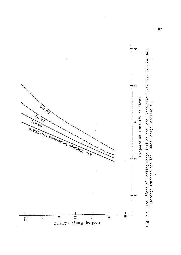
87

N.0 \

••,.0 n ...0 ›. ., .' e r• n

\

v %. s.».Se `S.

.... s„.

Se...\

.... \ss —s.-s...

... se.s. .....

S. \%,„,

J

-,....

.... ••••.s.— -...

oo.-s

..., ...,o. ••••

q...

••,.....

...N.

88

It is evident that water surface temperatures linearly affect the

depth of daily evaporation over various ranges (AT) with a slope of .0914

m/day- ° C (Fig. 3.10). One can see that the depth of evaporation in

Fig. 3.10 decreases with the pond cooling range (AT). This is due to the

fact that evaporation from the water surface is a function of the inter-

nal energy of water molecules which is related here to water surface

temperature. This indicates that, for a given heat load, the depth of

evaporation loss per day will be greater at higher surface temperatures.

However, the evaporation rate of the cooling pond will be greater at

lower outlet temperatures mainly because of the effect of the water sur-

face temperature together with the approach on the heat exchange coeffi-

cient of the water surface. Therefore, for a summer cooling design, it

is essential to consider the two aforementioned factors: evaporation

loss and depth of evaporation per day.

The computed annual evaporation losses for various design

criteria, represented in Fig. 3.11, increase over the range for any

given discharge temperature. Also, the annual evaporation losses for a

given heat load slightly change over various pond intake temperatures.

One should note that, for a given heat load, annual evaporation increases

as discharge temperatures decrease. As with the evaporation rate, this

is mainly because of the change in the heat exchange coefficient of the

cooling pond surface which is affected by water surface temperature

together with the approach. Therefore, optimum estimation of evaporation

should be based on annual evaporation rather than that occurring at any

of the particular design criteria. Variation in the evaporation rate

re)oo

••••

\• •••

• •

N •N s.

NN N •

N N •N

\ N N •

N °di •N a\°•,?.n

N 0'0:1...°/;ee,N N \

cNNN •

'NC N N •04T,N •••• •

N •41140N 41N0

14j se,0 N

N

N

N-•• %

N .% •N\ N

N

oc5

89

%

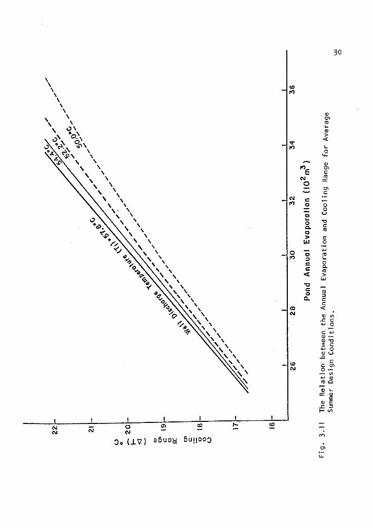
•ro, \ •

•

CO

0 \ ‘‘

\ •-

• \• \\ \\ •••

9 0

\• \\ \

'b. \‘ •\

o •cp. \

'C'...

• ‘Ns. • \s • •fi

-0 ‘ ‘‘ 00 N., N

v N., \ VI

‘,, ''nO

•

N ‘

91

over different times of the year, as indicated in Fig. 3.8, is not only a

result of the heat load but also a result of natural evaporation. This

was considered in all calculations.

The economic evaluation of cooling ponds must consider pond size.

The major cost in cooling pond construction is land cost. Figure 3.12

represents the cost of a pond for various design criteria of average

summer months. It is assumed that pond cost equals land cost; plus

operation cost which will not exceed .2% of the capital cost. The

capital cost of the cooling pond was evaluated as the cost of the area

multiplied by the cost of the land which is assumed to be $.21m2. There-

fore, capital cost is the major aspect in the economic analysis of

cooling ponds.

Spray Pond

A spray pond usually contains spray nozzles arranged at 6-10 feet

above the water surface. As the hot water ejects through the nozzle, it

breaks up into small drops, increasing the air-water interface. In addi-

tion to wind action and free convection, there is air movement to some

extent by the ejection action. The existence of water from several

nozzles crossing the wind stream reduces the horizontal air velocity.

Subsequently, the vertical velocity of the air along with the humidity of

the air participating in the heat exchange process is increased. The

heat and mass transfer coefficient increases as a result of the

increasing air-water interface. The heat dissipation by spray ponds over

cooling ponds may be as high as 3500 percent (Scofield and Fazzolare,

1971).

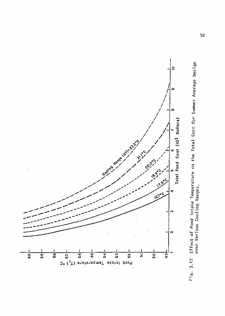
a)

0..... 4-)

0(o 17; I-

o a).. C.) .c

4-1

0

a)

92

Iri/

/I-.

//

// /

/ I-

/ /

.c.../ /1../

sr / / .C..V scr 1 /

a et)/ >/. I// .C.n /

4Z•e' / 0 ,aA /' / go /- / .

(:$•'/ / ,' oc,,e—(.4'

', / '' An..c) ,

„......,

/ . ,

, 6. .a

, A./ .

//.

lb

/ .

/ .

. °

..* . .

...-- .0'...* ...°. .

... .... . -* . ''... ..• - ....° .

-.-- . ...-- ... . .

.. .-• ... 0* . '•_

..n . ....n . -- --

..-- . ••• ''. . .. ..- ...... . ... .-- ._......•-•

.... —

o o) œ O U rn(c. in In to ICJ ul IA 10 in

00 ( I ) aJn4o.iedulai puod

93

The spray pond performance depends on the contact time between

the water droplets and air. In contrast to the cooling pond, the heat

exchange coefficient does not depend on the absolute air velocity. The

spray pond depends on the relative velocity of the air and water drop-

lets. Therefore, increasing the velocity of the water droplets by

increasing the nozzle pressure affects the relative velocity which

affects the heat transfer mechanism. This indicates that the spray pond

performance depends mainly on the design of the spray system.

This additional complexity of the spray pond makes it more

complicated to find sufficient methods of estimating the amount of heat

dissipation. There have been several attempts made to find such a solu-

tion. Badger and McCabe (1936) found that the spray pond could cool

0.6 to 0.8 m3 of 43.3 to 48.9 ° C water per hour per square meter to

21.1 ° C.

Scofield and Fazzolare (1971) tried to use a spray pond to cool

part of the water flowing to the pond using constant water and air flow

rates. They treated the spray performance as a cooling tower, neglecting

the effect of the climate ambient condition.

Therefore, field experimentation is required i- n order to evaluate

spray pond design. For this reason, further examination of this method

was not made.

Cooling Tower

A cooling tower is a device used to dissipate excess heat from a

thermal discharge. A water spray directed to the packing (or fill, which

is the material which forms the heat transfer surface within the tower

94

and over which the water is distributed in its passage down) increases

the contact surface between the water and the atmospheric air. This air

is drawn into the cooling tower by mechanical means (as in the case of

the mechanical draft tower) or by the density gradient between the out-

side air and that within the tower, and by the aerodynamic lift produced

by air passing over the chimney (as in the case of the natural draft

tower).

The cooling tower is the most efficient device used to reduce the

temperature of thermal discharges. The tower requires less land and also

provides better temperature control of the exit water than does the

cooling pond.

The natural draft tower has an advantage over the mechanical

draft tower in that it has low maintenance and operation costs. A dis-

advantage is the higher initial capital cost. Due to the fact that the

natural draft tower depends on natural wind flow, this type of tower is

usually built high and with broad sides facing the wind. Careful design

is necessary to ensure that the natural draft tower is stable in high

wind. Furthermore, due to the large height of this structure, there is a

need for additional pumping of the thermal discharge. Comparing the

total cost of the natural and the mechanical towers indicates that these

two types are comparable. However, the natural draft tower is unsuited

for regions of high humidity and high air temperature. Therefore, the

natural draft tower will not be presented in this paper.

95

Theory of Heat Transfer in CounterflowEvaporative Cooling

Counterflow is defined as the air flow direction, opposite to the

water flow direction. In evaporative cooling, the amount of air involved

in the cooling process is known. Air and water parameters are correlated

with each other by the heat and mass balance equation.

Air is moved opposite of flowing water in evaporative cooling.

The heat flux from the water surface can be expressed as (Berman, 1961):

(1) = Q0 p T 1 - (Q - dQ)C pT 2 (3.28)

Heat is dissipated from the water surface by contact, expended by

evaporation, and carried off by vapor. Therefore, equation (3.28) can be

rearranged as:

d(I) = K(Ts - T) + rB 1 (P - P) + dQC P

Ta s a 2

Comparing the right side of equation (3.28) and (3.29):

Q I C PdT = K(Ts

- Ta) + rB'(P s

- Pa

)

(3 .29)

( 3. 3 0 )

Ignoring the small reduction in water flow, at steady state, the

heat dissipation from the water equals the heat absorbed by air.

Assuming the specific heat of water equals unity, then equation (3.30)

can be written as:

(3.31)QdT = GdH

96

According to the theory of mass conservation, under steady-state

conditions the rate of mass leaving water by evaporation is equal to the

rate of increase of humidity:

dQ = Gd41

(3.32)

Heat transfer mechanisms are illustrated in Figs. 3.13 and 3.14.

Figure 3.13 illustrates the heat transfer process in the upper portion of

an evaporative cooler when the water temperature is higher than the dry-

bulb temperature. The humidity and temperature gradient decreases toward

the air interface, resulting in a reasonable amount of heat loss accounted

for by both latent and sensible heat loss.

On the other hand, when the water temperature is higher than wet-

bulb and lower than dry-bulb temperatures, the water continues to cool.

The temperature gradient increases toward the film, producing a flow of

heat from the bulk air to the water. In contrast, the humidity gradient

increases toward the water interface, causing mass-flow latent heat from

the water to bulk air. The sum of total heat from or to the interface

causes evaporation. This process is illustrated in Fig. 3.14.

Theory of Heat Transfer in Cooling Towers

The general concept of the cooling tower theory was first derived

by Merkel (1925). The use of the theory was described by Baker and

Shryock (1961).

The heat and mass transfer theory of cooling towers is well-

developed and can be found in numerous publications. It has been used

for cooling tower designs and evaluating cooling tower performance:

0

e-

97

a)0

9 8

C.)-e-

Co

••n•nn .monsoo ••••n••• 11n=11.

N\4'\N..\\.n,,

4-o

49-

99

= Qdt = K(T - T') + rfP(P s - P s ')

(3.33)

Consider a droplet of water falling through the tower within the

volume surrounded by air flowing past an interfacial film (Fig. 3.15).

It has been shown by Lichtenstein (1943) that, for a given unit area (a)

of a cooling tower having a volume dv, with an active surface area per

unit volume, the total heat flow from the water to the film interface is

written as:

4 = KLadv(T s - T') (3.34)

Heat losses from the interface to the bulk air as sensible heat

are expressed as:

dcp s = K(T 1 - Ta ) = KGadv(T' - Ta ) (3.35)

and the latent heat (heat of evaporation), assuming constant r:

rdQ = W(P s - Pa ) = rK'adv(W' - W) (3.36)

The enthalpy of moist air is the sum of the enthalpy of dry air

and water vapor:

H = Ha

+ WHv (3.36a)

= CaTa

+ W(r + CvTa

)

(3. 36 b)

Ts — dTsH W

G(tKg/hr)

A

q(Kg/h0

Ts

W dW

H + dH

100

if DifferentialI Volume dV

A/

// \

/ \

/ \

/ \

/ \/ \

T < i.T1 \CI / \

/ \/ \

\

// \

Sensible Heat

14 5 2 Ke adV (T' Ta )

\

W < tW" 11

// I

1Mass

I dC12 K l adV ( —W )I Bulk g

H< ;H' /

\ /

\ /

\ /%

N/

n•n ,

Bulk Air - ... ..........".., Interfacial Film

Fig. 3.15 Water Droplet for Heat and Mass-Transfer Simulation. -- From

Baker and Shryock (1961).

101

and

dH = C adTa + WC v

dTa + dW(r + CvTa) (3.36c)

The specific heat of humid air is defined as:

Cm = Ca

+ WCv

(3.37)

Substituting equations (3.36c) and (3.37) into (3.31):

QdT = GCmdTa

+ (r + C vTa1GdW (3.37a)

The first term of the right side of equation (3.37a) represents

sensible heat, whereas the second term represents latent heat.

Therefore:

KGadv(T 1 - Ta ) = GCmdT

(3.38)

From equation (3.31) and (3.36) the mass transfer becomes:

Wadv(W' - W) = GdW (3.39)

It has been found by Lewis (as reported by Baker and Shryock,

1961) that the rate of heat transfer by evaporation is analogous to heat

losses coefficient for sensible heat, which both processes depend on

temperature differences between the film surrounding immediately the

water droplets and bulk air flow over the surface. This relationship is

expressed as:

KG

KICm= 1.0

102

Therefore:

O s = K' GCmdVa(T' - Ta )

( 3 .4 o )

and

QdT = KGadv[C p (T' - Ta ) + [r + C v (T Ta )](W' - W)

(3.41)

The enthalpies of humid and saturated air are written as:

H = CmTa + Wr

(3.41a)

H' = CmT' + W'r

(3.41b)

Subtracting equation (3.41a) from (3.41b) with results substituted in

(3.41) yields:

QdT = K'adv(H' - H) = C vT(W' - W) (3.42)

The second term on the right side of the equation above is small

and can be ignored. Therefore, equation (3.42) becomes:

QdT = Kadv(H" - H) = GdH (3.43)

(H' - H) GH I

11 2dH KaV (3.44)

103

Assuming that Lewis' relationship is applied, equation (3.42) can

be solved by relating the air stream to the interfacial and substituting

KG and K' by the overall coefficients KG and K, respectively. Therefore:

The relationship can be applied with a certain degree of accuracy.

Equation (3.43) is applied to the local condition inside the

tower. Therefore, to determine the overall conditions of the tower per-

formance of an integration is required:

The enthalpy of both air and water in (3.43) are dependent on water

temperature. Therefore, equation (3.43) can be integrated over inlet and

outlet temperatures:

KaV2 dT

' (H' - H)T 1

(3.45)

The two equations are convertible with each other and they con-

form to the description of the transfer unit. Referring to (3.44), it

can be rearranged as:

1 04

H2

L = G/KAa f dH/(1-1 1 - H) (3.46)H 1

whereas:

H 2f dH/(H' - H)H 1

equals the number of transfer units (NTU), L equals packing height, and

G/KAa equals the height of the transfer unit.

The number of transfer units is defined as the height of the

packing required to achieve maximum heat transfer. The theoretical cal-

culation of NTU corresponding to a set of hypothetical conditions is

called the required coefficient. The same calculation can be applied to

a set of test conditions called the available coefficient of the tower.

The enthalpies' temperature relationships for counterflow towers

is given in Fig. 3.16. The water entering the top of the tower, with

bulk water temperature T 1 , surrounded by the interfacial film and having

an enthalpy of H' 1 , is represented by A. As the water moves down the

tower, its temperature decreases to T2 and enthalpy H' 2 . As the film

follows, the saturated curve is represented by point B.

In contrast, the air flow to the tower from the bottom with wet-

bulb temperature Twb and enthalpy H I is represented by point B'. As the

air moves up the tower, the temperature and humidity increase. Conse-

quently, the enthalpy H 2 is at point A'. The driving force at any point

In the heat transfer unit in the tower is the distance between the line

H I21

AirG

105

T2

Wafer Discharge Temperature °C

Fig. 3.16 The Effect of Temperature and Different Enthalpies between

the Air Flowing through the Tower and Saturated Enthalpy of

the Air at Local Water Temperature. -- From Fraas andOzistk (1965).

106

AB and A'B'. The form of equation (3.31) is dH = Q/G 3 .1. which leads to a

straight air operation line having a Q/G slope. It indicates that the

enthalpy of moist air varies linearly with water temperatures since the

derivation of log mean temperature differences depends on linear rela-

tionships between the enthalpy and the temperature of both mediums.

Solutions of Equations (3.44) and (3.45)

Knowing the mitai condition of air and water, the numerical

integration of equations (3.35) and (3.36) is performed. This can be

checked by subdividing the tower into a finite element of volume having

an equal temperature drop. Equations (3.44) and (3.45) can be written as:

Acp n = C pQdT = KadV(H' - H) m (3.47)

where (H' - H) m is the mean driving force over an increment of volume.

Therefore:

1 KaV = QC AT E

Ps (H" - H) m( 3. 48)

The value of the integral can be defined as the area under the

curve if 1/(H 1 - H) m is plotted versus the local water temperature as

shown in Fig. 3.17. The resulting quantities represent the value of the

tower characteristic KaV/Q which is a function of the inlet and outlet

wet-bulb air temperature and inlet and outlet water temperature.

The quantity of heat transfer within the cooling tower is a func-

tion of packing geometry and the water distribution system. The value of

a in equation (3.43) is not easy to determine but commonly ranges from

T2dT

Water Temperature °C

Fig. 3.17 The Approximation of Tower Characteristic by the Relation

between 1/(H" - H) and Local Water Temperature. -- From

Fraas and Ozisik . (1965).

1 0 7

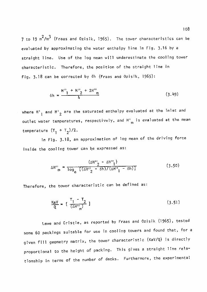
108

7 to 19 m2/m3

(Fraas and Ozisik, 1965). The tower characteristics can be

evaluated by approximating the water enthalpy line in Fig. 3.16 by a

straight line. Use of the log mean will underestimate the cooling tower

characteristic. Therefore, the position of the straight line in

Fig. 3.18 can be corrected by Sh (Fraas and Ozisik, 1965):

H" 1 + H"2 + 2H"m

Sh - 4(3.49)

where H'1 and H'

2 are the saturated enthalpy evaluated at the inlet and

outlet water temperatures, respectively, and H' m is evaluated at the mean

temperature (T 1 + T 2 )12.

In Fig. 3.18, an approximation of log mean of the driving force

inside the cooling tower can be expressed as:

(I-i"2 - AH" )

AH" =m loge

[(AH"2 - Sh)/(An - dh)]

Therefore, the tower characteristic can be defined as:

T1 - T2 1KaV = [

(ti-i")

(3.50)

(3.51)

Lewe and Cristie, as reported by Fraas and Ozisik (1965), tested

some 60 packings suitable for use in cooling towers and found that, for a

given fill geometry matrix, the tower characteristic (KaV/Q) is directly

proportional to the height of packing. This gives a straight line rela-

tionship in terms of the number of decks. Furthermore, the experimental

-*H"EquivalentStraight LineRelationfor H" n °.

H" A

Sh

HBH

S h

B'

AH

A'

10 9

T2

Local Water Temperature °C

Fig. 3.18 Method for Approximating Enthalpy Line by Straight Line to

Simplify the Tower Characteristic Calculation. -- From Fraas

and Ozisik (1965).

110

data showed that KaV/Q varies with some power of the Q/G ratio which can

be defined as:

KaV Q -n= .07 + BN( )

G(3.52)

Equation (3.52) gives the effect of fill geometry on tower per-

formance. This effect varies from one fill to another regardless of

inlet water temperature. Figure 3.19 shows the effect of a three fill

geometry matrix on the tower characteristic.

Pressure Drops in Cooling Towers

The pressure drop through the tower is a function of fill

geometry matrix, air flow rate, and water flow rate. These relationships

were analyzed by Fraas and Ozisik (1965) and can be expressed as:

AP= DG 2 ( 9- 67 x 1 0-5

Ya ) CQ G 2 9.67 10

- 5

e f Yeg () j—

a,R

(3.53)

where R is the mean free fall which is defined as the mean vertical dis-

tance that water droplets fall between slats. It is a function of free

flow area of the droplets and deck spacing. The value of Geg is equiva-

lent to the air loading corresponding to the mass velocity of the air

relative to falling water droplets. Therefore, it is a function of air

flow and free flow average distance.

111

1.65

1.60

4010 1.55

0—

Tr;1.50

77)1:45

1.40

30

135

1.30

1.2540 50 60

Tower Intake Temperature °C

Fig. 3.19 The Effect of Hot Water Discharge Temperature on TowerCharacteristic for Various Deck Fills. -- From Kelly andSwenson (1956).

112

Mechanical Draft Tower Costs

The cost of a cooling tower is affected by different factors,

such as its location and specific function. Cost varies from country to

country, city to city, as well as different sites within the city.

Therefore, there is no standard figure or formula to estimate cooling

tower costs.

The cost of cooling towers includes three major divisions:

initial cost, annual fixed costs, and operation costs. Since there are

no taxes, insurance premiums, or other similar expenses in Libya, annual

fixed costs will not be represented in this study. Furthermore, the

following cost analysis will partially depend on American methods of

estimating cooling tower costs since available data of cooling tower

costs in Libya do not exist.

There are two ways of expressing cost information: $/Kw of power

produced and S. Both depend on past data. Kolfate (1968) estimated the

cost of mechanical draft towers in nuclear power plants as $61Kw. The

cost increases if a closed approach is desired. He also estimated that

the fan of a mechanical draft tower consumed .8% of generating capacity.

Lockhart, Whitesell, and Catland (1955) correlated the data

obtained by Koulton for 32 mechanical draft towers. These data are pre-

sented in Figs. 3.20 and 3.21. The data have to be adjusted since costs

have doubled since 1955. Of the total generating capacity, 0.46% is con-

sumed by the fan and 0.85% of the total horsepower is used to operate the

pump and fan.

Approach =3.9°C

4.4°C5.0°C5.5°C

6.7°C

7.8°C

8.9°C10.0°C11.1 °C

10 14

Range AT °C

113

Fig. 3.20 Cooling Factor as a Function of Temperature Ranges and theApproach. -- From Carey, Ganley, and Maulbetsch (1969).

20 24

Wet Bulb Temperature °C

114

Fig. 3.21 The Relationship between the Wet-Bulb Temperature and

Wet-Bulb Coefficient. -- From Garey et al. (1969).

1 15

The capital cost is a function of location, land cost, design,

ambient conditions, tower installation, and other auxiliary costs. It

can be expressed as:

COS = 47.6 x QGM x K1413 x KX(IK) (3.54)

Capital cost is directly proportional to the range and flow rate and

inversely proportional to the approach.

Operation costs include: maintenance costs and horsepower cost.

Maintenance of cooling tower parts is essential to prevent any adverse

effects on the heat transfer capacity of the tower which depends on air

flow, water flow, and tower characteristics. Willa (1964) lists the

effects of poor maintenance.

The main system subject to change is the water distribution sys-

tem. Poor spray patterns usually are a result of corrosion, clogging,

algae, mud or oil accumulation which reduces the air flow rate, and

increases the static pressure through the tower.

Damages in the support structure and packing produce undesirable

water and air distribution which reduces the heat transfer coefficient.

Unfavorable performance sometimes occurs as a result of flow pulsation

within the fan.

The power cost is a function of approach; it increases as the

approach decreases. Therefore, the operation cost is inversely propor-

tional to the approach.

116

Computation Procedure

The method of computation basically depends on trial and error

procedures in which the temperature of the well water changes over

various ranges. Knowing the inlet and outlet of the water and water flow

rate, the heat load of the well water can be computed using equation

(3.28). Then the enthalpy of inlet and outlet air is calculated from the

ambient condition. Air flow rate is computed for specific enthalpy

using equation (3.31). However, recognizing that the fan is a constant

volume device, a slight change in air mass flow is a function of air

density. Therefore, density of inlet air is computed for given ambient

conditions. Air flow rate drive by the fan can be calculated when

density of the air is known. Pack height is calculated using the

analytical solution developed by Techbycheff (Smith and Maulbetsch,

1971). Knowing the deck height, the enthalpy of saturated air can be

determined which allows the computation of the saturated temperature of

outlet air. Next, the heat of evaporation is computed, thus permitting

the calculation of evaporative losses from the cooling tower. Total

horsepower needed to drive the fans can be calculated with knowledge of

the air flow rate.

A Fortran computer program was developed to accomplish the

computation. It is listed in Appendix B.

The heat load of well water expressed by equation (3.28) assumes

specific unit heat and neglects evaporation loss which is small compared

with total flow rate:

(Pp = Q(TI ". T2) (3.55)

117

Air flow rate is determined by equation (3.28) as (Garey et al.,

1 9 69 ):

(ho

(H2

- H1) -

G (3.56)

Since the specific heat of the air is a function of temperature,

the enthalpy of air can be expressed by a power series:

H(T) = a0

+ alT + a

2T2 + a

3T3 + a 4T

( 3.57)

where a0'

al'

a2'

a3'

and a4 are constants given by Smith and Maulbetsch

(1971).

The enthalpy of inlet air is computed at a given wet-bulb

temperature of the exit air. Outlet enthalpy is evaluated at the mean

temperature of the water.

The computation of specific humidity and partial vapor pressure

employs the following basic thermodynamic relations. Assuming water

vapor obeys the law of ideal gas, the specific humidity can be expressed

as:

.622 Pv (3.58)

P PB

or

.622 (RH x Pv")

W - pB - (RH x P

v")

118

Therefore, partial vapor pressure can be determined as:

P — v W + .622

pB

The saturated vapor pressure can be expressed in terms of

temperature by power series using Richard's (1971) approach:

,

P(T) = [a0 + a 1 T +

a 2T2 + a 3T 3 a 4T

4 + a 5T

5 j (3.59)

Inlet air density can be expressed by Bayle and Charles' law of

ideal gas (Severns and Fellows, 1949):

y = Pa/R

aT

= Pa/29.27(T + 273)

The size of cooling components are based on calculation of tower

characteristic KaV/Q. The method of calculation for this characteristic

is Techbysheff's approach which modified equation (3.51) for an approxi-

mate value of the numerical integration of equation (3.45) such that:

KaV — T

1 - T2 rD

1 R2 R 3

Ro (3.60)4 L"

where R1' R2' R3'

and R4 are the inverse difference between the satura-

tion enthalpy and the actual enthalpy evaluated as [T 2 + .1(T 1 - T 2 )],

[12 + .4(T 1 - T2)], [T 1 - .4(T 1 - 12 )], and [T 1 - .1(T 1 - 12)] (kcal/kg),

respectively.

119

The packing height of the tower necessary to give the above

characteristic was calculated using equation (3.52) where the number of

decks (N) can be expressed as:

N - packing height deck height

Therefore, equation (3.52) can be written as:

KaVDHT ( .7)PHT - Q

B ( i ) -nQ

(3 .6 1)

when the values of B and n are given by Fraas and Ozisik (1965) for each

specific deck height.

Knowing the packing height, the pressure drops through the tower

are computed using equation (3.53). Air loading (mass velocity) and the

equivalent air mass flow rate were found by Smith and Maulbetsch (1971)

as:

Ge

6= G/ 1

where ,51

is the ratio of the flow to the water loading. Equivalent air

mass (flow rate) is then computed (Smith and Maulbetsch, 1971). Thus,

equation (3.53) becomes:

9.67 x 10 -5] x [DGe 2

+ CQfGeq2kg/m

2pp = [(PHT/DHT) x Bya

(3-63)

120

where D and C are constants for a given pack height given by Fraas and

Ozisik (1964).

Water loss in cooling towers is not only dependent on the total

heat load, but also on the ratio of convectional heat transfer and latent

heat (evaporative) transfer. Water consumption predictions in mechanical

draft towers have been based on a rough rule of thumb (kg/555.5 kcal).

This approach neglects the effect of sensible heat transfer and the

atmospheric ambient conditions which can produce up to a 20% overestima-

tion of evaporative loss. The amount of water lost in the form of drop-

lets suspended in the exit air usually does not exceed 1 0/ of the total

water consumption.

Leung and Moore (1971) estimated the evaporation losses in

cooling towers of a power plant using the heat and mass transfer approach

where the cooling tower evaporation rate can be related to the air flow

rate and inlet and outlet specific humidity of the air.

Therefore, in order to solve for evaporation loss, assuming a

constant air flow rate mass ratio may reduce accuracy. Evaporation

losses are estimated by knowing the latent heat or heat of evaporation,

since the total heat dissipation is the sum of latent heat and sensible

heat. Thus, latent heat can be estimated by:

c e = ( r) 4) s

where cps = •24(Ta ' - Td )G, and where Ta 's are defined as the temperature

of saturated outlet air and can be expressed by a power series:

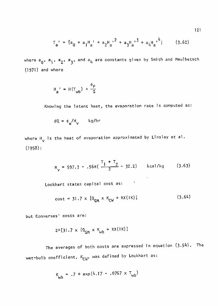
121

T' = [a + aH' + aH'2 + a

3a 4aH' 3 + aH

a'4

]0 la 2a

(3.62)

where a o , a l , a 2 , a 3 , and a 4 are constants given by Smith and Maulbetsch

(1971) and where

4)1,H' = H(T ) + —a wb G

Knowing the latent heat, the evaporation rate is computed as:

dQ = (I) e/Hv kg/hr

where Hv

is the heat of evaporation approximated by Linsley et al.

(1958):

T1 + T 2

Hv = 597.3 - .56H( - 32.2) kcal/kg (3.63)

2

Lockhart states capital cost as:

cost = 31.7 x x KCW + KX(IK)]GM (3.64)

but Converses' costs are:

2*(31.7 x (Q0 x Kwb + KX(IK)]

The averages of both costs are expressed in equation (3.54). The

wet-bulb coefficient, Kcw , was defined by Lockhart as:

b . .7 + exp(4.17 - .0767 x Twb

)

122

produced in Fig. 3.20. The cooling factor by Lockhart, KX(IK), obtained

from a curve fit of data, is produced in Fig. 3.21.

Knowing the outlet air density air flow rate, the driven air flow

rate (G f ) is computed by:

With driven air flow rate and pressure drop through the tower known, the

horsepower required to drive the fan is then computed as:

FHP = (G f x AP)/(4562 x .80)

where fan efficiency is assumed as 0.8. There is no need for the water

pump to raise water to the top of the tower so the only horsepower

needed is for the fan. Assuming maintenance cost is .1 of capital cost,

operating cost can be computed as:

OPC = .1 x COS -I- THP x .03

Therefore, the total cost is the sum of operating costs and capital

costs.

Results and Discussion

The same criteria employed for the cooling pond were used for the

mechanical draft tower. Results were computed at sea level elevation.

The highest elevation of the investigated area was 200 m above sea level

which had a negligible effect on the results of computations. The

computed evaporation rate expressed as the percentage of well flow rate

123

for summer design criteria of differing discharge temperatures and

cooling demands is shown in Table 3.2. One can see that the evaporation

rate significantly changes over cooling demands, but slightly changes

over intake temperatures. Variation in evaporation rate for discharge

temperatures changes linearly over various ranges (AT) with a magnitude

of 224.5 kg/1- ° C, as shown in Fig. 3.22. Evaporation rates for the tower

and of the cooling pond display comparable form. However, the evapora-

tion rate of the pond at any given design criteria in this study is

always greater than the evaporation rate of the tower with similar

design criteria. This is related to the fact that, unlike the tower,

evaporation rate of the pond is affected by natural evaporation loss. In

contrast to the cooling pond, the evaporation rate of the tower for a

given heat load increases over intake temperatures. This is primarily

because higher intake temperatures increase the enthalpy of air flowing

through the tower, resulting in a higher saturated air capacity.

As illustrated in Fig. 3.23, a higher evaporation rate will occur

when the highest wet-bulb temperature is combined with the lowest rela-

tive humidity. Monthly changes in wet-bulb temperatures and relative

humidity are shown in Fig. 3.24. The figure clearly demonstrates that

the highest evaporation rate occurs during summer months. When employing

parameters of ambient wet-bulb temperature and relative humidity, it is

obvious that when the incoming air is at a high wet-bulb temperature

coupled with low relative humidity, the evaporation loss is high and

sensible heat transfer is low. In contrast, when the incoming air is at

Table 3.2 Tower Evaporation Rate in Terms of WellDischarge Percentage for Summer DesignConditions.

WellDischarge

Temperature( ° C)

Cooling Range (%)

16.7 17.8 18.9 20.0 21.1 2.22

48.9 2.62 2.79 2.97 3.14 3.31 3.49

50.0 2.62 2.79 2.97 3.14 3.31 3.49

51.1 2.62 2.80 2.97 3.14 3.32 3.49

52.2 2.63 2.80 2.97 3.15 3.32 3.49

53.3 2.63 2.81 2.98 3.15 3.32 3.50

54.4 2.64 2.81 2.98 3.16 3.33 3.50

55.5 2.64 2.82 2.99 3.16 3.34 3.51

56.7 2.64 2.82 2.99 3.17 3.34 3.51

57.8 2.65 2.82 3.00 3.17 3.35 3.52

58.9 2.65 2.82 3.00 3.17 3.35 3.52

60.0 2.64 2.82 3.00 3.18 3.35 3.53

124

\

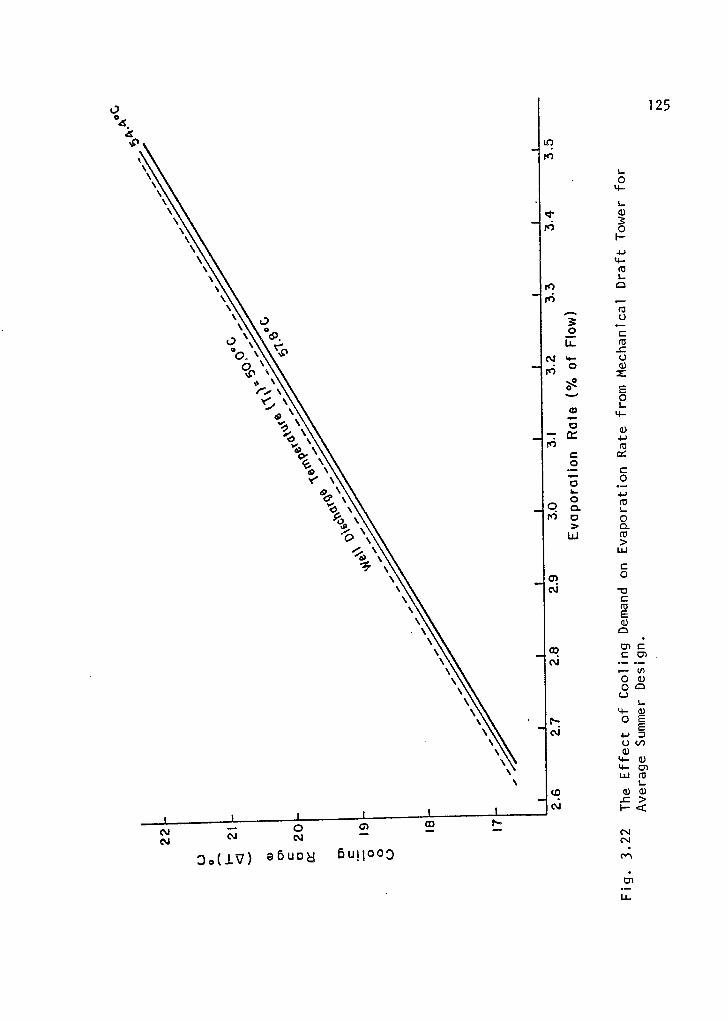
ê0. \

LI-C

CCO

0 \ CV 4- 1.1

eil \0 (1)

o \rri Z

,-

Y \e, E..• \

../ ....... 0

Ci) ‘‘.0

1-

'1', '•nn• LI...

iff ‘(1.)

1,

"".: CC

61 \ In

J,)

c•ro

‘ c cc

er, \0

ell, \0

0

';:),.. ‘

04•J

Y.0 ‘

0

IllS-

O0 0

..." \ > CL

0 ‘ LLi CO

...." \>

o) \Li)

12504

4./

C:1

•—

O

CO

{id).U

0 \0

•-

0

-C3Cro

Cl•

Cri CC tD1

•-• cnO a)O a)

126

, / .

, ,/

, ,I /, I /

t , i I% 1 k% t \. \,

. •

. •\.. , \ \,. , \.„ •, , \% 1 \

t \'1 1

1, 1 IiI

1

1I

t Î II

% 1

% 1

1 1

1 1 I1

/ / i

/ // /, ,/ /coo CJ f /° / e0/

,

CO. s 0 f / /

I Ai/Sj/

oCT /I CS/

•i /

Cy riv//

/ / / CV,f /

/f f /

/ 0/f I /

/ /// / /

/f /

/ //f /

If / I /

f / I I

i / /I Ifi 0 I

I / / /

Dec.

Nov.

Oct.

Sept.

Aug.

July

June2

May

Apr.

CO.

Mar.

Feb.

Jan.

2.5 2:7 2.9 3.1 3.3

3.5

Evaporation Rate (% of Flow)

Fig. 3.23 Variation of Evaporation Rate over the Year in Percentage ofFlow Rate for Various Cooling Ranges (AT) at 57.8 ° C WellDischarge Temperature.

(%) 9nitoi3 8

r-

oO

1

D2

1

o

0, ainolgadwai

127

128

a low wet-bulb temperature coupled with high relative humidity, the

evaporation loss is low and sensible heat transfer is high.

In Fig. 3.25, unlike the pond, the annual evaporation loss of the

tower increases over intake temperatures of a given heat load. For any

given discharge temperature and range, annual evaporation loss from the

tower is smaller than the cooling pond. This is related to the fact that

the cooling tower is not affected by the solar radiation. Therefore,

there is no accounted evaporation occurring in the cooling towers under

natural conditions. Although annual evaporation loss of the towers was

computed for only 65% of the operating time, the total annual evaporation

loss of the pond is higher than that of the tower regardless of seepage.

A family of curves in Fig. 3.26 approximates a linear relation-

ship of the approach (the difference between the tower outlet water

temperature and wet-bulb temperature) on pack height. A low approach

coupled with a low saturated air enthalpy difference requires greater

contact time demanding higher packing construction.

Figure 3.27 shows the total cost of the cooling tower affected

exponentially by well discharge temperatures for various ranges. This

effect fluctuates from $0.62 per 555.5 kcal at a 60 ° C well discharge

temperature -- 16.7 ° C range (AT) to $0.17 per 252 kcal at a 48.88 ° C well

discharge temperature -- 22.2 °C range, compared with the cooling pond's

total cost of $.20 per 250 kcal to $.67 per 252 kcal for the same design

criteria. Capital cost of the tower and of the cooling pond is similar

with the exception of operating costs. Difference in operating costs is

mainly due to the effect of the approach (difference between wet-bulb

\ Crl.--roof...„,

n o =

/ \ cni -J c

d \c

•••;›,\

cO

<

L

v \4••• (1)

.9 ‘0

V. \'6 I—

00:,_

A) \ o.

Y \ 0 c0,,

> 0.9 w

-0 •• C U

m 0,

Es,;:_,=C s..

•cr c a) c

ctrY) 1...

••*c a)

— EO a)O I-L)

a)4- (7)O /-

CO4-) -CO 0O in

4- —4- CILI-I

pcn

(I)

I- 3

0. (IV) abuo8 6uH000 .

O

1/14.)V)

\

tn

\—10

\\ ..-.. C

\0

\

fe)E

.+-,

\Os.1 (0C L\0 0

O 0. \ v:. .....—

asa

0 • a,

045 , 0 \ 41

>

0 \co t.LJ

SI \CL)(r)

12 9

13 0

/ Il /a ./ ccus

// / --

-C C

/Ii

I.-

I / VI *-C -

0 0

//

II4-

6- 01 C..)

(13/

Qi / CO N.

41 /N/ .-- /

.c0.... Q3/

al / //Is-/ 0

ii I0_

/ /I </ 0-

44/ / / o •/ / c

o0/

//

//

3 cllcu (n

I +-1 clCV

/ o c/•/

/ _cl n)

o.=4-ni

i LI-// o/

// 01

-C/

/ .-/ 0

=//

• C

01

/

/ C.) -Y

O U

/I/ 0 0-

(13

//

C., a)

et(j/ o/ o

c.) / /,.=

/ 4-I

Pi 18. -o`1.i/ 13- / 0 1 P I 0

oc.) eL

cro

4,4 / cz,./ 0-, co / O <

L.a)

0

1 3 1

V)

0

oC.1

re)0

•••n•

(1)oo

0°./ .0'./ ___ ___ .•'.....-'oe .."' ....... I'.

...'" ..•••• / .... .....••••".. ...° .0... / ....

...••••..•••• /

•

I.••• , ••• ../

••• as./ a// ••••/ /

.....••••

CI?) /

i/ /0)! t.)/e

11di

//

,//

/

//

// C.) /

/ 0/ /

,.... /•.-o /

/ if(1/ //

/ / /// ///

/0/ /1

/ / ii 0) /aCJ /

/ / // n4) . //

/ /// //

// // /

// /

/ / /

// // •

/ AO.

/ //

/ / / / /

/ / .0 "

/ / .• ' " /#

0/ 0//o

• './ ../. / ...

.# e

0.

In Lc)

Oo (II) e nloiadwai e1DuI Jarnoi

13 2

temperature of inlet air and outlet water temperature) on horsepower

required to operate the fan at any given design criteria. It is evident

that, at a low wet-bulb temperature and high well discharge temperature

coupled with a low cooling range (AT), the difference between the

saturated enthalpies leaving and entering the tower is high. Therefore,

the air flow rate through the tower will be small. On the other hand,

when the wet-bulb temperature of incoming air is high and the mean water

temperature throughout the tower is low, heat gained by air is at its

minimum and air flow rate at its maximum. Subsequently, air flow rate

throughout the tower decreases as mean water temperatures increase,

causing lower pressure drops. This demonstrates that, at a low air flow

rate, a reduced amount of horsepower is required, implying that the maxi-

mum amount of horsepower is necessary in summer months, compared with the

remainder of the year. In contrast to operating cost, capital cost of

the tower reaches its maximum in winter and minimum in summer.

Total cost of the cooling tower was computed for a 25-year life

which is assumed to be a well's lifetime. Calculation does not include

pump cost. It assumes well pressure is sufficient to raise water to the

top of the tower equivalent to the pressure computed for irrigation in

Chapter 2 of this research.

Conclusions and Recommendations

Conclusions

By comparing the results of the cooling tower and cooling pond,

it is clear that the cooling tower would be the most water efficient

133

method. The higher evaporation in the pond due to the effect of solar

heating is absent in the cooling tower system. If seepage is also con-

sidered, then pond water consumption could be as much as two or three

times that of the cooling tower. Even though initial pond construction

costs may be half of the tower's, there are other factors that must be

taken into consideration in determining the optimum method of cooling

thermal waters:

I. The Wadi's width is an average of only 0.5 km. The project area

is 10 km long. This would mean that the cooling ponds would

require about 1.5% of this valuable agricultural land.

2. The soil profile is alluvial to 1 meter deep, underlain by marly

limestone of low permeability. A pond without lining will be

subject to lateral subsurface outflow. The resultant drainage

problem in adjacent agricultural lands will increase overall

operations cost.

3. Lining the cooling with concrete will increase the cost of the

pond to as much as 20 times the cost of the tower.

4. The capital cost of power for tower operation will not be a major

factor because the project has already constructed its own power

station to supply the needs of the pumping and irrigation

activities as well as for residential requirements.

The total cost and annual evaporation losses required for dissi-

pating 1.9 x 1010

kcal-kg/year or for a discharge temperature of 57.77°C

and a 20 ° F cooling range for 70% of operation time by using the two

134

cooling methods is summarized in Table 3.3. The evaporation rate of the

two systems using similar average summer conditions is found in Table 3.4.

As it has been mentioned in the first part of this research, well

discharge temperatures range from 55-58 °C. If we assume that the tower

reduces the temperature to 38 ° C, and that a further reduction in tempera-

ture to 30 ° C occurs due to heat dissipation in the irrigation system and

in the soil surrounding the plants, the water that will arrive at the

roots of the plant will be suitable for the plant species utilized in the

project.

In conclusion, based on the assumptions made, the cooling pond

may not be considered as a viable method. The results of this study indi-

cate that, given the two alternatives, the cooling tower system is by far

the most efficient and economically optimal method for treating thermal

water for agricultural purposes.

Furthermore, with some modification, the results of this study

can be used for designing the cooling system of power plant condenser

discharged water.

Recommendations

This investigation presented two cooling system analyses. The

comparison between the two systems was made only on the basis of simpli-

fication and general empirical solutions coupled with some assumptions.

The applier of this result should be aware of the variation in climate

data during the months.

The empirical analysis used for cooling pond design in this

investigation was developed mainly by Brady et al. (1969) from a field

Table 3.3 Comparison between the Tower Cooling Pond of57.8 ° C Discharge Temperature and 20 ° C Coolingper Well Range.

Cooling Method

TotalCost

(s)

CapitalCost

(s)

Area AnnualRequired Evaporation

2 3(m) Cm)

Cooling tower 7085 5346 80 25,964.7

Cooling pond 2746 2650 4249 30,220

135

Table 3.4 Evaporation Rate of 57.8 ° C Discharge Temperatureand 20 ° C Cooling Range.

Evaporation

Evaporation

Natural

Rate Rate

Evaporation

Cooling Method

(%)

(m/yr)

(m/yr)

Cooling tower 3.17

Cooling pond 3.57

8.7 1.7

136

study in South Central United States. The accuracy of the empirical

formula for the study area should be verified by field measurements. The

cooling tower study was based on a simplified thermodynamic analysis. It

should be known that the author was not capable of gathering all the

necessary field data for making the check on the sensitivity of the

calculations.

Therefore, the following study is recommended to be undertaken:

1. A field experiment should be conducted to study the feasibility

of using spray pond or spray modules as other means for lowering

the high well water temperature.

2. A small-scale model of the cooling systems (pond and tower)

should be constructed and the following investigation should be

made:

a. Compare the mathematical models with the field data for the

two cooling systems, pond and tower.

b. Determine the effect of daily meteorological fluctuations on

cooling pond performance.

c. Correlation analysis should be run to compare the actual

evaporation with the computed one.

d. Determine the effect of climatological instability on cooling

pond performance.

3. Make an economic evaluation of the two systems. It is obvious

that an adjustment to the economic cost should be made on the

basis of Libyan data.

137

4. An agricultural experiment should be made to determine the effect

of various water temperatures on plant growth and on productivity

in the project area.

APPENDIX A

DEFINITION OF SYMBOLS

Symbol Definition Units

A Water surface area.m2

Ca

Specific heat of air. kcal/kg

Cm Specific heat of humid air. kcal/kg

Specific heat of water. kcal/kg

Cv

Specific heat of vapor. kcal/kg

C BBrunt's coefficient. kcal/kg

Equilibrium temperature. °C

f(W) Wind function. W/m mm Hg

FHP Fan horsepower.

G Air flow rate. kg/hr

H' Enthalpy of moist air in a bulk water

temperature. kcal/kg

H" Enthalpy of moist air at water interface

temperature. kcal/hr

Hal

Enthalpy of inlet air. kcal/kg

Ha2Enthalpy of outlet air. kcal/kg

H Heat of vaporization. kcal/kgV

H1

Enthalpy of moist air entering the tower. kcal/kg

H2Enthalpy of moist air leaving the tower. kcal/kg

138

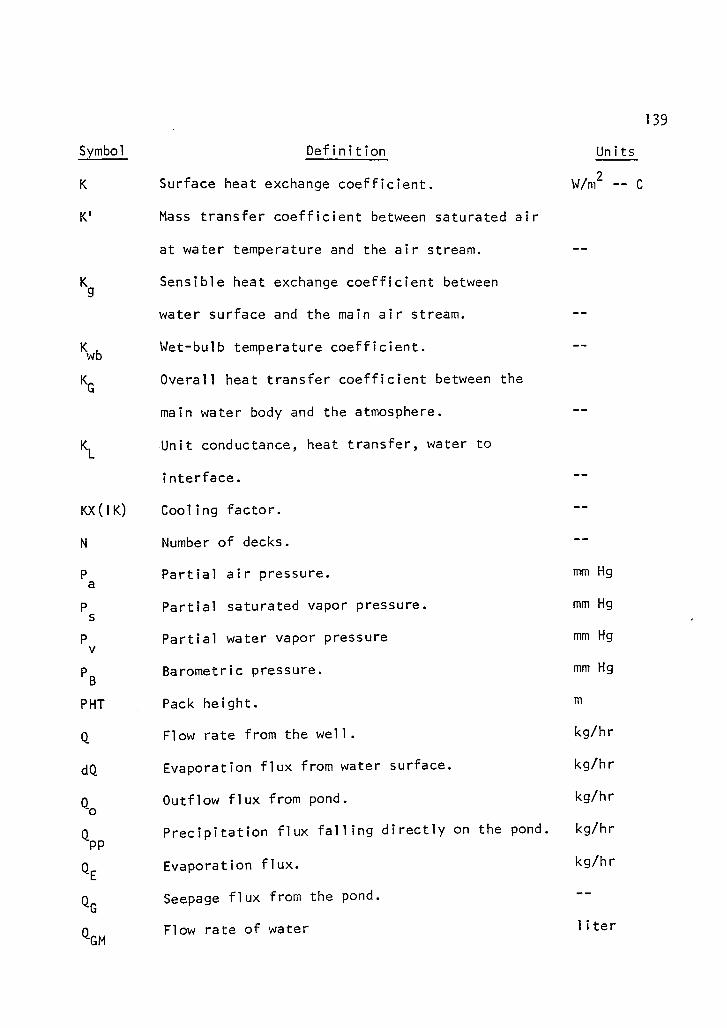
139

Symbol Definition Units

Surface heat exchange coefficient. W/m2 -- C

K' Mass transfer coefficient between saturated air

at water temperature and the air stream.

Sensible heat exchange coefficient between

water surface and the main air stream.

bWet-bulb temperature coefficient.

KG Overall heat transfer coefficient between the

main water body and the atmosphere.

KL

Unit conductance, heat transfer, water to

interface.

KX(1K) Cooling factor.

Number of decks.

Pa

Partial air pressure. mm Hg

Ps

Partial saturated vapor pressure. mm Hg

Pv

Partial water vapor pressure mm Hg

PB

Barometric pressure. mm Hg

PHT Pack height.

Flow rate from the well. kg/hr

dQ Evaporation flux from water surface.kg/hr

QOutflow flux from pond. kg/hr

o

Qpp

Precipitation flux falling directly on the pond. kg/hr

QEEvaporation flux. kg/hr

QGSeepage flux from the pond.

QGMFlow rate of water liter

140

Symbol Definition Units

Q I Inflow flux from thermal source kg/hr

QR Runoff flux to the pond. kg/hr

r Latent heat of the medium. kcal/kg

Ra ,Rv Universal gas constant of dry air and vapor.

Medium temperature °C

T' Interfacial film temperature. °C

7r- Mean excess temperature. °C

Ta Air temperature. °C

Td

Dew point temperature. °C

T. Excess temperature at lake intake. °C

T n Natural water temperature. °C

To

Excess temperature at discharge point. °C

Ts

Water surface temperature. °C

TwbWet-bulb temperature °C

T 1Water thermal discharge temperature. °C

T2Outlet water temperature or evaporative cooler

water discharge temperature. °C

V Volume of pond water. m3

Wind velocity. m/sec

Specific humidity of the bulk air.

W' Specific humidity of air-water interface.

W" Saturated specific humidity.

W 1Specific humidity of intake air.

W2Specific humidity of outlet air.

141

Symbol Definition Units

Vapor pressure difference proportionally

factored to temperature difference. mm Hg/ ° C

y Water density. kg/m3

YaAir density. kg/m3

Yv Vapor density. kg/m 3

AP Pressure drops.

6 Emissivity of water surface. .97

Am Wavelength.

a Stefan-Boltzmann constant.

(1) .9 Long-wave atmospheric radiation incident on

pond surface. W/m2

(1)abLong-wave reflected atmospheric radiation by

pond surface. W/m2

(I) brLong-wave radiation from the pond surface. W/m

2

(1)cEnergy lost or gained by convection from the

water surface. W/m2

dHeat flux by conduction. W/m

2

(i) eEnergy transfer from the water surface by

evaporation. W/m2

Outflow energy flux. W/m2

(1)o

(I) Well heat rejection.w/m2

(I) Energy flux by precipitation. W/m2

PP

Solar radiation incident on pond surface. W/m2

(PnNet absorbed heat. W/m

2

4) s

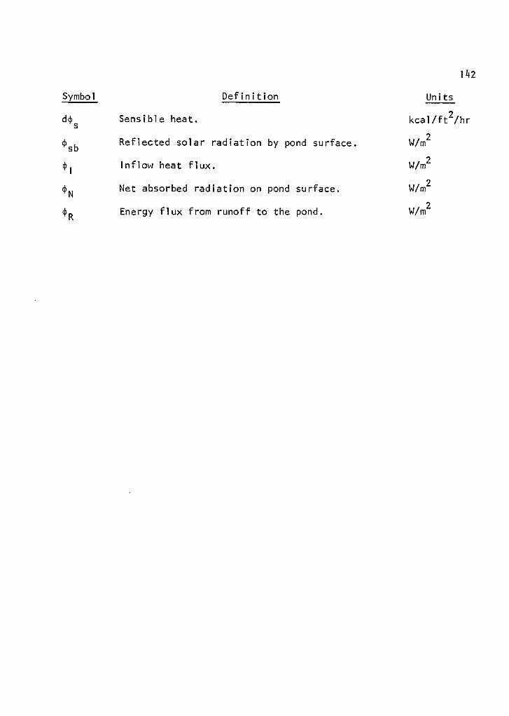
142

Symbol

g'sb

4) 1

(I) N

4) Ft

Definition

Sensible heat.

Reflected solar radiation by pond surface.

Inflow heat flux.

Net absorbed radiation on pond surface.

Energy flux from runoff to the pond.

Units

kcal/ft 2/hr

W/m2

W/m2

W/m2

W/m2

APPENDIX B

COMPUTER PROGRAM

143

THE PROGRAME IS IN ENGLISH UNITSPROGRAME POND (INPOT,OUTPUT)DIMENSION MONTH(1(4),EMONTH( 14) , AIRT( 14) ,DEWT (14) ,EVAPR (14) ,X V

5 AP (14) , HRAD (14) , WIND (14) ,EQUALT (14) , AREA (14) , TOTCOS (14) ,EXCOEF$ (14) ,HRJ (14) , WSURFT (14)

REAL INTT (14)FLO:4=79.17264E5 *.8

• READ GENERAL INFORMATION OF THE AMBIANT CONDITIONDO 35 L=1,1READ 100, (MONTH (I) , AIRT (I) , DEWT (I) , HRAD (I) , WIND (I) ,EQUALT (I)

5,1=1,1 14)100 F3RMAT (3 X,A2,2F5.1,F7.1,3X,2F5.1)• PRINT GENERAL INFORMATION OF THE AMBIANT CONDITION

PRINT 200, (MONTH (I) ,AIRT (I) , DEWT (I) ,[(RAD (I) ,WIND (I) , EQUALT (I)$, 1=1,1 (4 )

200 FORMAT (15X,A5,5F10.2)• CALCULAT THE MONTHLY EQUALIBRIUM TEMP.

DO 15 I=1,14WIN DF=70+.07*WIND (I) **2

13

AVET= (DEWT (I) +EQU ALT (I) ) /2.

BETA=.255—.0085*AVET+.000204*AVET**2COEF=15.7+ (BETA+. 26) *WINDFEQUALT1= (—COEF+SQRT (COEF**2—. 2* (—HEAD (I) +1801— (BETA*DEWT (I)

$. 26*AIRT (I) )*WINDF) ) )/. 1EQDIF=EQUALT (I) —EQUALT1IF (EQDIF. GT. —.5. AND. EQDIF.LT..5) GO TO 201EQUALT (I) =EQUALT1GO TO 13

201 EQUALT (I) =EQUALT115 CONTINUE

DO 35 K=30,40,2WELLT=KHRJ (14) =FLOW*WELLTLPAGE=2DO 35 J=120,140,2DIST=JDO 30 1=1,14

APR° ACH= DIST—WELLT—EQUALT (I)WINDF=70+.07*WIND (I) **2WSURFT (I) =HRJ (/) / (FLOW*ALOG ( (DIST—EQU ALT (I) )/APROACH)) +EQUALT (I)AVET= (WSURFT (I) +DEWT (I) ) /2BETA=.255—.0085*AVET+.000204*AVET**2EXCOEF (1) =15.7+. 05* (EQUALT (I) +WSURFT (I) ) + (BETA+. 26) *WINDF

• CALCULÂT THE REQUARED AREAAREA (I) =FLOW/EXCOEF (I) *ALOG ( (DIST—EQU ALT (I) ) /APROACH)

• CALCUAT THE TOTAL COST WHICH EQUAL TO THE OPERATION COST +CAPTAL COS:COST=AREA (/) *0.06OPCOS=COST*. 002TOTCOS (I) =COST+ OPCOS

• COMPUT THE MONTH OPERATION TEMPRETURWSURFT (I) ,--- DIST—WELLT/2.

26 AVET= (WSURFT (I) +DEWT (I) ) /2.BETA=.255—.0085*AVET+.000204*AVET**2EXCOEF (I) =15.7+. 05* (EQUA LT (I) +WSURFT (I) ) + (BETA+.26)*WINDFSURTDIF=DIST—NSURFT (I)IF (SUR TDIF.LT.. 5) GO TO 29siSURFT1=EQUALT (I) +HRJ (I) / (EXCOEF (I) *AREA (I) )

I 44

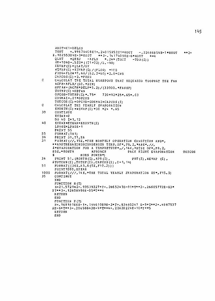
145

HOUT=H1+DELHSTOUT =.99674408E1+.24015952E1*HOUT -.22686654E-1*HOUT **2+

3.10255304E-3*HOUT **3-.14174090E-6*HOUT **4QLAT =QREJ -AFLR *.24*(TOUT -TDB(I))HV=1040 - .523*((71+12)/2.-90)XEVAP(I)=QLAT/HVWEVAP(I)=XEVAP(I)/(FLOW) *100FUDG=FLOW*7.48/(62.2*60)*2.0*CWBCAPCOS(I)=3.*FUDGCALCULÂT THE TOTAL HORSPOWR THAT REQUARED TOOPRAT THE FANACFd=AFLR/(60.*DIN)HPFAN=(ACFM*DELP*5.2)/(33000.*FANEF)TOTHP(I)=HPFANOPCOS=TOTHP(I)*.75* 720*12*25*.65*.03COS1AI=.01*OPCOSTOTCOS(I)=OPCOS+COSMAI+CAPCOS(I)CALCULÂT THE YEARLY EVAPORATIONE1ONTH(I)=WEVAP(I)*30 *24 *.65

30 CONTINUEEYEAR=0DO 40 1=1,12

40 EYEAR=EYEAR+EMONTH(I)LPAGE=LPAGE+1PRINT 55

55 FORMAT(1H1)36 PRINT 31,T1,RA31 FORMAT(//,15X,*THE dONTHLY OPERATION CONDITION AND*,

**ANDTHEMAXIMUMCONDENSER TEMP.OF*,F8.2,*ARE*,//,S*EVAPORATION FOR A TEMPRETURE*,/,16X,*RISE OF*,F8.2,$5X,*MOUTH APROACH PACK RIGHT EVAPORATION TOTCOS

HORS POWER*)34 PRINT 51,(MONTH(I),APR(I), PHT(I),WEVAP (I),

STOTCOS(I),TOTHP(I),CAPCOS(I),I=1,14)51 FORMAT((36X,A5,6(5X,F10.2)))

PRINT1000,EYEAR1000 FORMAT(///,14X,*THE TOTAL YEARLY EVAPORATION IS*,F15.5)35 CONTINUE

ENDFUNCTION H(T)H=21.572142-.93539227*T+.2865243E-01*T**2-.26605772E-03*

$T**3+.12608996E-05*T**4RETURNENDFUNCTION P(T)P=.16818166E-1+.14461089E-2*T+.83460247 E-5*T**2+.4987537

SE-6*T**3-.20658843E-9*T**4+.22620224E-10*T**5RETURNEND

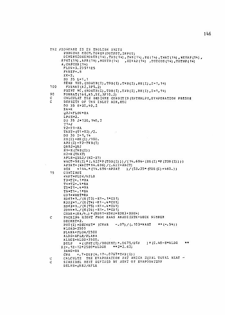
THE PROGRAME IS IN ENGLISH UNITSPROGRAM MECH.TOWER(OUTPUT,INPUT)DIMENSIONEMONTH(14),TDB(14),TWB(14),RH(14),TWAT(14),WEVAP(14),SPHT(14),APR(14),MONTH(14) ,XEVAP(14) ,TOTCOS(14),TOTHP(14)3,CAPCOS(14)FLOW=3.29511E5FANEF=.8XK=2.DO 35 L=1,1READ 100,(MOUTH(I),TDB(I),TWB(I),RH(I),I=1,14)

100 FORMAT(A2,3F5.2)PRINT 90,(MONTH(I),TDB(I),TWB(I),RH(I),I=1,14)

90 FORMAT(16X,A5,5X,3F10.2)• CALCULAI THE DESIGNE CONDITIN(ENTHALPY,EVAPORATION PRESUR• DENSITY OF TUS INLET AIR,ETC

DO 35 K=30,40,2RA=KQRJ=FLOW*RALPGE=2.DO 35 J=120,140,2T1=JT2=11-RATAXT=(T1+T2)/2.DO 30 1=1,14RH(I)=RH(I)/100.APH(I)=T2-TWB(I)QREJ=QRJH1=H(TWB(I))H2=H(TAXT)AFLR=NEJ/(H2-H1)WACT=RH(I)*(.622*P(TDB(I)))/(14.696-(RH(I)*P(TDB(I))))APSAT=(WACT*14.696)/(.622+WACT)DIN =144.*(14.696-APSAT )/(53135*(TDB(I)+460.))

15 CONTINUEWART=FLOW/AFLRT3=T2+.1*RAT4=T2+.4*RAT5=T1-.4*RAT6=T1-.1*RACO1=WART*RARDH1=1./(H(T3)-H1-.1*C01)RDH2=1./(H(T4)-H1-.4*C01)0DH3=1./(H(T5)-H1+.4*C01)RDH4=1./(H(T6)-H1+.1*C01)CHAR=(RA/4.)*(RDH1+RDH2+RDH3+RDH4)

• PACKING EIGHT FROM RAAS ANDOZISTK-DECK NUMBERDECKHT=2.PHT(I)=DECKHT* (CHAR -.07)/(.103*WART **(-.54))WLOAD=2500PLANA=FLOW/2500ALDG=AFLR/PLANAALDGE=ALDG+3500.DELP =((PHT(I)/DECKHT)*.0675/DIN )*(0.4E-8*ALDG **

32+.1E-12*2500*ALDGE **2*2.62)RANG=RACW8 =.7+EXP(4.17-.0767*TWB(I))

• CALCULTE THE EVAPORATION RAT WHICH EQUAL TOTAL HEAT -

C SINSIBEL HEAT DEVIDED BY HEAT OF EVAPORATIONDELHS=QREJ/AFLR

146

1 47

DIFSURF=VISURFT (I) -WSURFT1IF (DI FSUR F.GT.-.5. AND. DI FSURF. LT..5) GO TO 204WSURFT (I) =wsuRFr1GO TO 26

204 WSURFT (I) =WSURFT1

29 EXCEST=DIST-EQUALT (I)INTT (I) =DIST-WELLT

291 HRJ (I) =FLOW* (DIST-INTT (I)IF (HRJ (I) . GT. HRJ (14) ) HRJ (I) =I-1RJ (14)X=EXP (-EXCOEF (I) *ARE A (I) /FLOW)ENTT1=EQUALT (I) +EXCEST*XENTTDIF=INTT (I) -ENTT 1IF (ENTTDIF.GT.-.5.AND.ENTTDIF. LT..5) GO TO 293INTT (I) =ENTT 1GO TO 291

• CALCULÂT THE SURFACE TENRETUR AND BETA ,AND THE HEAT REJECTION BYTHE LAKE IF THE SPRAY IS REQUARED

• 293 SPRAY=DIST-W ELLTIF (INTT (I) .LT.SPRAY) GO TO 295POND HRJ=HRJ (I) * (DIST-INTT (I) ) /WELLTWSURFT (I) =EQUALT (I) +PONDHRJ/ (EXCOEF (I) *AREA (I))AVET= (ASURFT (I) +DEWT (I) ) /2HET k=.255-.0085*AVET+.000204*AVET**2

• CALCULAT THE HEAT OF EVAPORATION AND EVAPORATION RATE295 HVAPOR=1041.25-. 5629* (WSURFT (I)-9C)

XVAP (I) =BETA* (WSURFT (I) -DEW T (I) )*WINDF*AREA (I) / (HVAPOR)

EVAPR (I) =XVAP (I) / (62.2*AREA (I) )EMONTH (I)=EVAPR (I) *720

30 CONTINUEEYEAR=0DO 40 1=1,12

40 EYEAR=EYEAR+EMONT H (I)LPAGE=LPAGE+1IF (LPAGE. LT.2) GO TO 34PRINT 55

55 FORMAT (1H1)LPAG E=0

34 PRINT 31,WELLT, DIST31 FORMAT (//,15 X,* THE MONTHLY OPERATION CONDITION AND *,*

$THE MONTHLY MAXIMUME WELL TEMP.*,F8.2, 4ARE*,//,

$*OPERATIOM AT TEMPRETIUR*,/, 16X ,*RISOF*, F8.2,$5X,*MONTH WSURFCE INTAK K EQUALIBRIUN EVAP.

HRJ*)DO 33 1=1,14IF (INTT (I) . LT. SPRAY) ICC=" "

IF (INTT (I) .GT.SPRAY) ICC="+"PRINT 32, ICC, MONTH ( I) , WSURFT (I) ,INTT (1) , EXCOEF (I) ,EQUALT (I) ,

SEVAPR (I) ,AREA (I) , TOTCOS (I)

32 FORMAT( (34X,A1,A5,4 (5X,F5.1) ,5X,F10.5,5X, F10.2,1210.2))

33 CONTINUEPRINT 1001,EYEAR

1001 FORMAT (///,14X,*THE TOTAL YEARLY EVAPORATION IS*,F15.5)

35 CONTINUEEND

REFERENCES

Anderson, E. R. 1952. Energy budget studies in water-loss investiga-tions: Volume I, Lake Hafner studies. U. S. Geological SurveyCircular 229.

Badger, W. L., and W. L. McCabe. 1936. Elements of Chemical Engineering, 2nd edition. New York: McGraw-Hill Book Co.

Baker, D. R., and H. A. Shryock. 1961. A comprehensive approach to theanalysis of cooling tower performance. Journal of Heat Transfer,

August.

Berman, L. D. 1961. Evaporative Cooling of Circulating Water. NewYork: Pergamon Press.

Boersma, L. L., E. W. R. Barlow, and K. A. Rykbost. 1972. Use ofreactor cooling water from nuclear power plants for irrigation of

agricultural crops. Water Resources Research Institute, Oregon

State University, April.

Bowen, I. S. 1926. The ratio of heat losses by conduction and byevaporation from any water surface. Physical Review, Vol. 27,June.

Brady, D. K. 1969. Surface heat exchange at power plant cooling lakes.Edison Electric Institute, Publication No. 69-901, The JohnsHopkins University, Baltimore, November.

. 1970. The Dissipation of Heat from Thermal Discharge.Baltimore: Johns Hopkins University Press, April.

Brady, D. K., W. L. Grave, Jr., and J. C. Geyer. 1969. Surface heatexchange at power plant cooling lakes. Cooling Water Studies for

Edison Electric Institute, Publication No. 69-901, The JohnsHopkins University, Baltimore, November.

Branko, J., and R. Brikish. 1974. Chemical quality of ground water.C. A. D.

Campbell, M. D., and J. H. Lehr. 1973. Water Well Technology. NewYork: McGraw-Hill Book Co.

Cummings, N. W., and B. Richardson. 1927. Evaporation from lakes.Physical Review, Vol. 30, October.

148

149

Ediger, J. E., and J. C. Geyer. 1965. Heat exchange in the environment.

Cooling Water Studies, Edison Electric Institute, Publication

No. 65-902, The Johns Hopkins University, Baltimore.

Ezzat, M. A. 1977. The development of the Egyptian western desert.

Ministry of Irrigation, Cairo, April.

Fraas, A. P., and M. N. Ozisik. 1965. Heat Exchange Design. New York:John Wiley & Sons, Inc.

Garey, J. H., J. T. Ganley, and J. S. Maulbetsch. 1969. A survey andeconomic method of alternative methods for cooling condenser dis-

charge in thermal power plants, Task 1 report: Survey of large-scale heat rejection equipment. Dynatech Report No. 849,July 21.

Gaudrazi, G. 1972. Geology and mineral resources of Libya. U. S.Geological Survey report.

GEFL. 1972. Reconnaissance ground water survey in the central part ofLibya. Tripoli, Libya.

General Water Authority. 1972. Ground water in Hun graben. Tripoli,Libya, September.

. 1973. Ground water evolution in North Gefara Plateau.Tripoli, Libya.

. 1974. Flowing test in Wadi Zam-Zam. Tripoli, Libya.

Hogan, W. T., A. A. Liepins, and F. E. Reed. 1970. An engineering-economic study of cooling performance. Federal Water Quality

Control Administration, R & D Report No. 16130DFX, May.

Hutchinson, G. D. 1957. A Treatise on Limnology. New York: John Wiley& Sons, Inc.

Israelson, O. W., and V. E. Hansen. 1962. Irrigation Principles and Practices. New York: John Wiley & Sons, Inc.

Jones, J. R. 1964. Ground water hydrology in Sintica. U. S. Geological

Survey report.

Johnson Division (Universal Oil Products Co.). 1972. Ground Water and Wells. St. Paul, Minnesota: Edward E. Johnson, Inc.

Kelly, N. W., and L. K. Swenson. 1956. Comparative performance of

cooling tower packing arrangement. Chemical Engineering Progress,Vol. 52, p. 263.

150

Koberg, G. E. 1963. Methods to compute long-wave radiation from the

atmosphere and reflected radiation from a water surface. U. S.

Geological Survey Professional Paper.

Koberg, G. E., G. E. Harbeck, and T. Hughs. 1959. The effect of theaddition of heat from a power plant on the thermal structure and

evaporation of Lake Colorado City, Texas. U. S. Geological

Survey Professional Paper No. 272-B.

Kolfate, T. D. 1968. How to beat the heat in cooling water.Electrical World, October 14.

Langhaar, J. W. 1953. Cooling pond may answer your water coolingproblem. Chemical Engineering, August.

LeBosquet, M. 1946. Cooling water benefits from increased river flows.Journal of New England Water Works Association, Vol. 60, No. 2,June.

Leung, P., and R. E. Moore. 1971. Power plant cycles for dry coolingtowers. Paper presented at the ASCE National Water ResourcesEngineering meeting, Phoenix, Arizona, January 12.

Lichtenstein, J. 1943. Performance and selection of mechanical draftcooling towers. Trans. ASME, Vol. 65, p. 779.

Lima, D. O. 1936. Pond cooling by surface evaporation. Power, March

Linsley, R. K., M. A. Kohler, and J. L. Paulhus. 1958. Hydrology for Engineering. New York: McGraw-Hill Book Co.

Lockhart, F. J., J. M. Whitesell, and A. C. Catland, Jr. 1955. Coolingtowers for the power industry. American Power Conference.

Marciano, J. J., and G. E. Harbeck. 1954. Mass transfer studies in

water-loss investigation: Lake Hafner Studies. U. S. GeologicalSurvey Professional Paper 269.

Merkel, F. 1925. Verdunstungskuehlung. VDI Forschungsarbeiten (Berlin),No. 275.

Pasternak, D., M. Twersky, I. Borovic, Y. de Malach, and E. Rappaport.

1975. Use of geothermal brackish water for soil warming andvegetable irrigation. International Symposium on Brackish Water

as a Factor in Development, Beer-Sheva, Israel, January.

Richards, J. M. 1971. Simple expression for saturation vapour pressure

of water in range 50 ° to 140 ° . Brit. J. Appl. Phys., Vol. 4,pp. L15-L18.

15 1

Scofield, F. C., and R. A. Fazzolare. 1971. Nuclear power plant heat

rejection in arid climates. American Nuclear Society Winter

Meeting, Miami Beach, Florida, October 2.

Severns, W. H., and J. R. Fellows. 1949. Heating, Ventilating, and Air-

Conditioning Fundamentals. New York: John Wiley & Sons, Inc.

Smith, N., and J. S. Maulbetsch. 1971. A survey of alternative methods

for cooling condenser discharge water: Selection, design, and

optimization. Water Pollution Control Research Series, 16130DHS,

January.

Stanford, D. W., and G. B. Hill. 1970. Cooling towers principles and

practices. Carter Thermal Engineering Limited.

Sverdrup. H. U. 1937-38. On the evaporation from the oceans. Journal of Marine Research.

Theis, C. V. 1935. The relation between the lowering of piezometricsurface and the rate and duration of discharge of a well using

ground water storage. Trans. Am. Geophys. Union, 16th Annual

Meeting.

Throne, R. F. 1951. How to predict lake cooling action. Power,

September.

Velz, C. J., and J. J. Cannon. 1960. Forecasting heat losses in ponds

and streams. Journal W. P. C. F., Vol. 32, No. 4, April.

Willa, J. L. 1964. Effect of maintenance on cooling tower performance.Materials Protection, October.

Zarazzer, D. 1975. Ground water quality in the central region of theLibyan Arab Republic. General Water Authority, Tripoli.

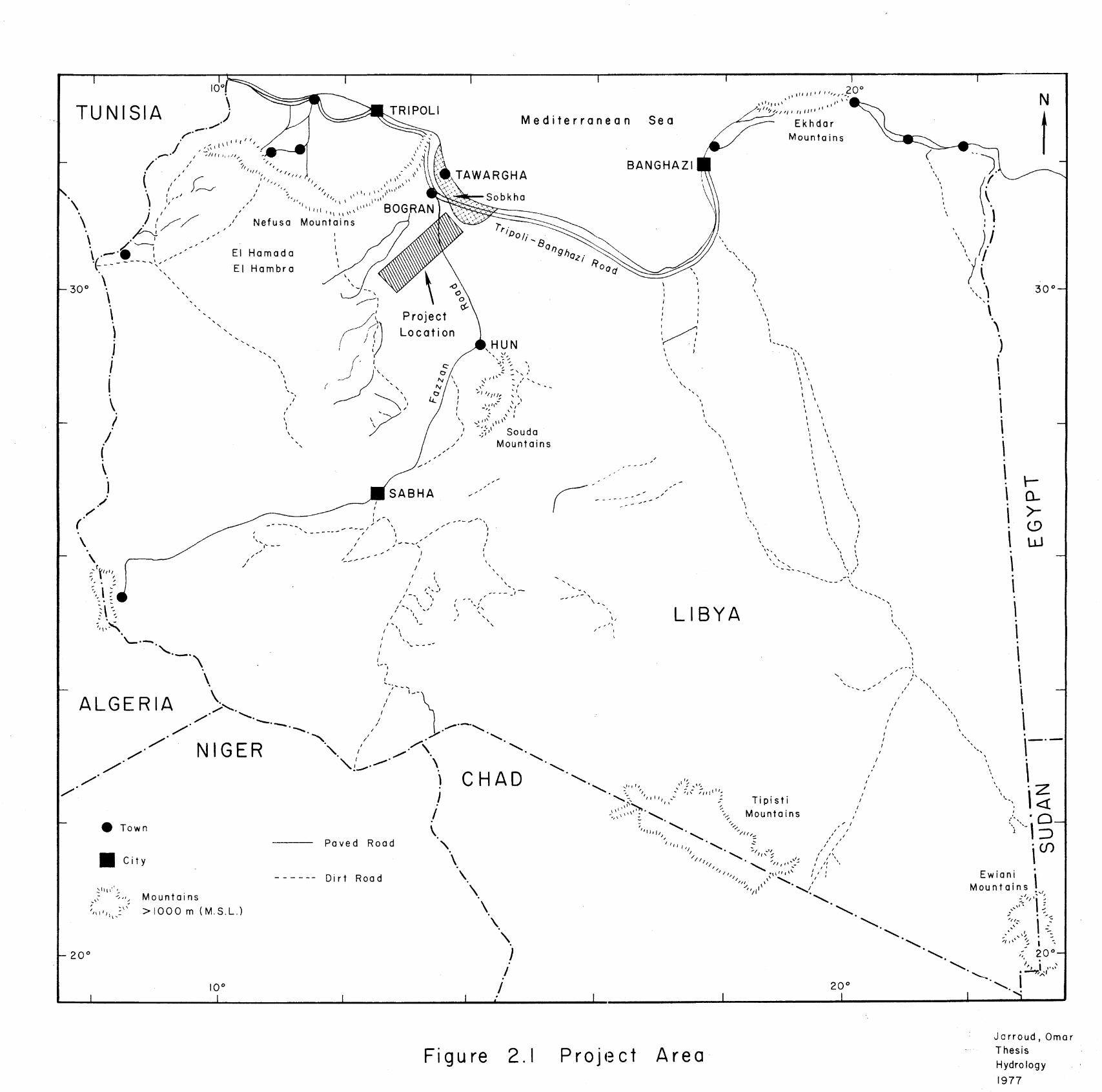
TUNISIA10°

TRIPOLIMediterranean Sea

1i „ if h/ 1s , 20 0

• •0 , 1110 si‘• 1 1/ 5////1 Is

EkhdarMountains

'So nghazi

it? 0 a cie •

Sobkha

30°—

/

s.

••

I/

s".••71 , • /„

TipistiMountains

/I .t •

/ / •‘,,

S.

, /,,

11‘

//I

./1 •

LIBYA

BANGHAZITAWARGHA

f"•/ 0

1\ 1 , 1 t 'f ,,

.

/ ,

.

,, ,

. , ',I, ,,,,,,_..., i

„

./.

.--

II '// \/

/ r'/ '/

/

/\ :

,

‘I

(/ i' / I

I ,,, , 1 1/, %•

• /

,0•\ •

\\ 1/ '''

\i

/ /

i 1 /I,

•

I

1I -.1,.-. — '0 i ,..-

•El Hamada 1

t__.__ ,.. , ,, - 1'El Hambra

30°

ProjectLocation

„ s , • n 1• Is ,,,

''‘i Iii,„,,,„k ' BOGRAN///,/„, 0

t k I

""k"/

Nefusa Mountains

.1 •

HUN

ALGERIA

NIGER

• Town

u City

Mountains

>1000 m (M.S.L.)

20°

10°

\.

•

-- Dirt Road

.1 CHAD

/Paved Road

• s.

/ •1

•

s.

, IZI .Ct

g

1 ID. "

J

EwianiMountains,

•_it—

s.•- 1 -• I• 5/ • ...

/'Ia• •, /

,; 20°—, „

20°

I1

Jarroud, OmarThesis

Hydrology

1977

Figure 2.1 Project Area