
Rights / License: Research Collection In Copyright - Non ...9042/eth-9042-02.pdf · abh angt und...
105
Research Collection Doctoral Thesis Optical Detection of the Hyperfine Interaction in a Positively Charged Self-Assembled Quantum Dot Author(s): Studer, Priska Barbara Publication Date: 2014 Permanent Link: https://doi.org/10.3929/ethz-a-010209092 Rights / License: In Copyright - Non-Commercial Use Permitted This page was generated automatically upon download from the ETH Zurich Research Collection . For more information please consult the Terms of use . ETH Library
Transcript of Rights / License: Research Collection In Copyright - Non ...9042/eth-9042-02.pdf · abh angt und...

Research Collection
Doctoral Thesis
Optical Detection of the Hyperfine Interaction in a PositivelyCharged Self-Assembled Quantum Dot
Author(s): Studer, Priska Barbara
Publication Date: 2014
Permanent Link: https://doi.org/10.3929/ethz-a-010209092
Rights / License: In Copyright - Non-Commercial Use Permitted
This page was generated automatically upon download from the ETH Zurich Research Collection. For moreinformation please consult the Terms of use.
ETH Library
DISS. ETH NO. 21916
Optical Detection of the Hyperfine Interaction
in a Positively Charged
Self-Assembled Quantum Dot
A dissertation submitted to the
ETH ZURICH
for the degree of
Doctor of Sciences
presented by
Priska Barbara STUDER
Dipl. Phys.ETH Zurich
born 28th of October 1984
citizen of Schupfheim LU
Accepted on the recommendation of :
Prof. Dr. Atac Imamoglu, examinerProf. Dr. Klaus Ensslin, co-examiner
2014

c
Abstract
In this dissertation, optical studies of the interaction between either a single hole
spin or a single electron spin confined to a self-assembled InGaAs quantum dot
(QD) with the nuclear spin ensemble of the host material are presented. QDs are
semiconductor structures that allow for a charge carrier confinement in all spatial
directions; this leads to a quantization of the electronic states. Dipole allowed tran-
sitions between the electronic states enable an optical spectrum similar to the one
of atoms. In fact, a QD consists of 105 atoms with nonzero nuclear spin. A single
hole spin or electron spin confined to the QD couples to this ensemble of nuclear
spins via hyperfine interaction. Optical orientation of the electron spin polarization
can be transferred to nuclear spins via hyperfine interaction, leading to dynamic
nuclear spin polarization (DNSP). On the other hand the nuclear spin polarization
acts back on the electron spin, causing an energy splitting of the electronic spin lev-
els. This characteristic can be exploited to optically measure DNSP by performing
spectroscopy.
In the first part of this thesis, we investigate the evolution of nuclear spin polar-
ization in a transverse magnetic field via a single QD electron spin. While in a
magnetic field along the growth direction a pronounced DNSP is expected, in a
transverse magnetic field the nuclear spin polarization should vanish because of the
Larmor precession of the electron. Experimentally, nuclear spin polarization com-
pensates transverse magnetic fields Bx up to ∼1.7T. Therefore, the orientation of
the nuclear spin polarization has to be mainly perpendicular to the optically de-
fined electron spin polarization. To further investigate this anomalous behavior, we
develop a pump probe technique that allows to fully characterize the nuclear spin
polarization as function of Bx by resonant spectroscopy. The aim is to find out
whether the evolution of nuclear spin polarization in transverse magnetic fields can
be mapped to quantum optics models. We find that the nuclear spin polarization
in transverse magnetic fields strongly depends on the sample structure and is very
likely an inherent property of self-assembled InGaAs QDs due to their strain.
In the second part of this thesis, coherence properties of single hole spins confined
in a QD are studied with time resolved measurements. By optically charging the
QD in an n-doped field-effect structure we can benefit from the superior electronic
properties of such devices. We find a coherence time T ∗2 of 240ns which is an or-

d
der of magnitude larger than what was previously measured in p-doped samples.
Additionally, we observe that the hole spin coherence measurements are strongly
influenced by nuclear spins.

e
Zusammenfassung
In dieser Arbeit werden optische Studien der Interaktion zwischen einem einzel-
nen Lochspin oder einem einzelnen Elektronenspin, der in einem selbstorganisier-
ten InGaAs Quantenpunkt (QP) eingeschlossen ist, mit dem Kernspinensemble des
umgebenden Materials vorgestellt. Quantenpunkte sind Halbleiterstrukturen, die ei-
ne dreidimensionale raumliche Eingrenzung von Ladungstragern erlauben, was eine
Quantisierung der Elektronenzustande ermoglicht. Erlaubte Dipolubergange zwi-
schen den Elektronenzustanden fuhren zu einem ahnlichen optischen Spektrum wie
in einem Atom. Im Gegensatz zu einem Atom besteht ein Quantenpunkt jedoch
aus 105 Atomen, die alle einen endlichen Kernspin besitzen. Ein einzelner Lochspin
oder Elektronenspin im Quantenpunkt koppelt zu diesem Kernspinensemble uber
die Hyperfeinwechselwirkung. Deshalb kann die optisch verursachte Polarisation des
Elektronenspins auf die Kernspins ubertragen werden, was zu einer dynamischen
Kernspinpolarisation (DKSP) fuhrt. Andererseits bewirkt die Hyperfeinwechselwir-
kung eine Aufspaltung der Energiezustande des Elektronenspins, wenn das Elektron
in Kontakt mit den spinpolarisierten Kernen steht. Diese Eigenschaft wird verwen-
det, um den Grad der DKSP mit Hilfe von spektroskopischen Methoden optisch zu
bestimmen.
Im ersten Teil dieser Arbeit wird die Entwicklung von Kernspinpolarisation in einem
transversalen Magnetfeld mit Hilfe von einem einzelnen Elektronenspin im Quan-
tenpunkt untersucht. Wahrend in einem Magnetfeld entlang der Wachstumsrich-
tung des QPs eine starke DKSP erwartet wird, sollte die Kernspinpolarisation in
einem transversalen Magnetfeld aufgrund der Larmorprazession des Elektrons ver-
schwinden. Experimentell kann eine Kompensation des externen Magnetfeldes Bx
durch die Kernspinpolarisation bis zu ∼1.7T festgestellt werden. Dazu muss die
Kernspinpolarisation mehrheitlich senkrecht zur optisch definierten Polarisation der
Elektronenspins orientiert sein. Um diesen ungewohnlichen Polarisationsmechanis-
mus der Kernspins zu studieren, wird eine Pump-Probe Technik entwickelt, die eine
vollstandige Charakterisierung von der Kernspinpolarisation als Funktion von Bx
mit Hilfe von resonanter Spektroskopie erlaubt. Das Ziel dabei ist herauszufinden,
ob die Entwicklung der Kernspinpolarisation in einem transversalen Magnetfeld mit
quantenoptischen Modellen beschrieben werden kann. Wir stellen fest, dass die Kern-
spinpolarisation in transversalen Magnetfeldern sehr stark von der Probenstruktur

f
abhangt und sehr wahrscheinlich eine inharente Eigenschaft von selbstorganisierten
InGaAs QP aufgrund ihrer Gitterverspannung ist.
Im zweiten Teil dieser Dissertation werden die Koharenzeigenschaften von einzel-
nen Lochspins in QP mit zeitaufgelosten Messungen untersucht. Indem der QP
optisch mit einem einzelnen Lochspin in einer n-dotierten Feldeffektstruktur ge-
laden wird, konnen wir von den ausgezeichneten elektronischen Eigenschaften dieser
Struktur profitieren. Wir messen eine Koharenzzeit T ∗2 von 240ns, die verglichen
mit vorhergehenden Messungen in p-dotierten Strukturen um eine Grossenordnung
langer ist. Daruber hinaus stellen wir eine starke Beeinflussung der Lochspin
Koharenzmessungen durch Kernspins fest.

Contents g
Contents
Title a
Abstract d
Zusammenfassung e
Contents g
List of symbols and abbreviations i
1. Introduction 1
1.1. Motivation and scope of this thesis . . . . . . . . . . . . . . . . . . . 2
2. Self-assembled Quantum Dots and Nuclear Spins 5
2.1. Charge tunable self-assembled Quantum Dots . . . . . . . . . . . . . 5
2.1.1. Growth of self-assembled quantum dots . . . . . . . . . . . . . 6
2.1.2. Quantum dot level scheme and optical selection rules . . . . . 7
2.1.3. Charge control . . . . . . . . . . . . . . . . . . . . . . . . . . 9
2.1.4. Quantum confined Stark effect . . . . . . . . . . . . . . . . . . 11
2.2. Nuclear Spins in Quantum Dots . . . . . . . . . . . . . . . . . . . . . 13
2.2.1. Electron and Hole Spin System . . . . . . . . . . . . . . . . . 13
2.2.2. Nuclear Spin System . . . . . . . . . . . . . . . . . . . . . . . 14
2.2.3. Isotropic and Anisotropic Hyperfine Interaction . . . . . . . . 16
2.2.4. Electron Spin Decoherence . . . . . . . . . . . . . . . . . . . . 18
3. Experimental Methods 21
3.1. Photoluminescence . . . . . . . . . . . . . . . . . . . . . . . . . . . . 21
3.2. Resonant Rayleigh Scattering . . . . . . . . . . . . . . . . . . . . . . 22
3.3. Resonance Fluorescence . . . . . . . . . . . . . . . . . . . . . . . . . 24
3.4. Pump Probe Measuring Methods . . . . . . . . . . . . . . . . . . . . 24
3.4.1. Optical detection of Nuclear Spin Polarization . . . . . . . . . 25
3.4.2. Pump Probe Method with Resonant Rayleigh Scattering . . . 26
3.4.3. Pump probe Method with Resonance Fluorescence . . . . . . 34

h Contents
4. Nuclear Spin Polarization in Transverse Magnetic Fields 37
4.1. Introduction . . . . . . . . . . . . . . . . . . . . . . . . . . . . . . . . 37
4.2. Hanle experiment . . . . . . . . . . . . . . . . . . . . . . . . . . . . . 38
4.3. Anomalous Hanle Effect . . . . . . . . . . . . . . . . . . . . . . . . . 39
4.4. Hanle measurements for samples with different electron spin lifetimes 41
4.5. Resonant measurements on a 35nm tunnel barrier sample . . . . . . . 45
4.6. Resonant measurements on a 25nm tunnel barrier sample . . . . . . . 46
4.6.1. Gate properties . . . . . . . . . . . . . . . . . . . . . . . . . . 47
4.6.2. Resonance fluorescence background . . . . . . . . . . . . . . . 48
4.6.3. Extraction of the resonance positions . . . . . . . . . . . . . . 49
4.6.4. Transition between Overhauser shift and hole Zeeman splitting 50
4.7. Discussion . . . . . . . . . . . . . . . . . . . . . . . . . . . . . . . . . 55
5. Coherence of Optically Generated Hole Spins 59
5.1. Introduction . . . . . . . . . . . . . . . . . . . . . . . . . . . . . . . . 59
5.2. Spectroscopy on X+ . . . . . . . . . . . . . . . . . . . . . . . . . . . . 61
5.3. Initialization and Readout . . . . . . . . . . . . . . . . . . . . . . . . 62
5.4. Rabi Oscillations . . . . . . . . . . . . . . . . . . . . . . . . . . . . . 63
5.5. Ramsey measurements . . . . . . . . . . . . . . . . . . . . . . . . . . 65
5.6. Spin Echo measurements . . . . . . . . . . . . . . . . . . . . . . . . . 68
5.7. Discussion . . . . . . . . . . . . . . . . . . . . . . . . . . . . . . . . . 70
A. Appendix A
A.1. Experimental Setup . . . . . . . . . . . . . . . . . . . . . . . . . . . . A
B. Bibliography I
Acknowledgements XI
Curriculum Vitae XIII
List of Figures XV

List of symbols and abbreviations i
List of symbols and abbreviations
gel,h,ex g-factor (for electron, hole and exciton, respectively)
j Total angular momentum (spin and orbital)
l Orbital angular momentum
Ai Hyperfine coupling constant of nucleus i
Bel Knight field
Bext External magnetic field
Bloc Local dipolar nuclear field
Bnuc Overhauser field
EF Fermi energy
Ii, I i Nuclear spin operator and quantum number
N Number of quantum dot nuclei
Q Nuclear quadrupolar moment
S, S Electron spin operator and projection on z−axis
T1 Spin relaxation time
T2,(T ∗2 ) Spin dephasing time (ensemble averaged)
Vg Applied gate voltage
γi Gyromagnetic ratio of nucleus i
ν0 Unit cell volume
ρ+c (ρ−c ) Circular polarization of PL light (under σ+- (σ−-) polarized excitation
σ+(σ−) Circular light polarization of positive (negative) helicity
σx Linear light polarization along x
ωQ Quadrupolar coupling strength
Ψ Electron wave function
Ωel Electron Larmor frequency
∆EOS Overhauser shift
∆EZel,e,ex Zeeman splitting (for electron, hole and exciton, respectively)
↑, ↓ (⇑, ⇓) Electron (hole) spin up, electron (hole) spin down

j List of symbols and abbreviations
1eV = 1.6 · 10−19 J 1 electronvolt
e = 1.6 · 10−19 A·s Electron charge
g0 = 2 Free electron g-factor
~ = 6.582 · 10−10 µeVs Reduced Planck’s constant
µB = 58 µeV/T Bohr magneton
k = 86 µeV/K Boltzmann constant
µ0 = 4π · 10−7N/A2 Permeability of free space
As Arsenic
CB Conduction band
CCD Charge coupled device (camera)
DNSP Dynamical nuclear spin polarization
CPT Coherent population trapping
FWHM Full width at half maximum
Ga Gallium
HH Heavy hole
In Indium
LH Light hole
MBE Molecular beam expitaxy
PL Photoluminescence
PLE Photoluminescence excitation
QD Quantum dot
QI Quadrupolar interaction
RF Resonance fluorescence
SIL Solid immersion lens
SNR Signal to noise ratio
Ti Titanium
VB Valence band
Xn Exciton of charge n

Introduction 1
1. Introduction
We all use modern electronic devices in daily life for work, communication and
entertainment. Year by year, the computing power of such devices grows. One
of the main reasons for this development is the miniaturization of the electronic
components. Hence an increasing amount of functionality can be realized on the
same area of the computer chip. As a consequence a computer processor consists of
millions of transistors, where the smallest have a gate length of 10nm. The ability
to fabricate devices at such small length scales has also inspired many research
areas. The growth and study of objects where at least one of the spatial dimensions
extends to only a few nanometers is called Nanotechnology. If objects are made
smaller and smaller, the classical description fails at low temperature and quantum
mechanical effects play an important role.
The study of charge carriers that are confined in low dimensions led to the discovery
of interesting electrical and optical properties such as the Aharanov-Bohm effect [1],
Coulomb blockade [2] and the quantum Hall effect [3]. In this thesis we focus on
semiconductor structures with a confinement in all spatial directions, quantum dots
(QD). On one hand, a QD shows a discrete energy spectrum and optical properties
like an atom, on the other hand it is an object consisting of 104 − 105 atoms. The
confinement allows for a study of the interaction of a single electron or hole with
its environment. One example is the interaction with a nearby electron or hole
reservoir that results in interesting many-body physics [4–6]. Furthermore, the
electron spin in a QD couples to the nuclear spins of the atoms the QD consists of
via hyperfine interactions [5, 7, 8].
Single electrons confined in a QD are considered as promising candidates for
the use as spin qubits in quantum information processing [9, 10]. Compared
to atoms, the on-chip realization is promising for the scalability of the system.
Additionally, QDs exhibit long spin lifetimes and coherence times due to the weak
interaction with the environment [11]. This is absolutely crucial for quantum
information storage. Last but not least, the coherent optical control of electron
spins in self-assembled QDs allows for a fast manipulation of the quantum state on
picosecond timescales [12, 13]. Therefore a prospering research field was established
which addresses the problem of initialization, manipulation and readout of the

2 Introduction
electron spin [14–16].
However, a single electron spin in a QD is not completely isolated from its envi-
ronment. On the one hand, coupling to the environment is needed to manipulate
and read out its state and on the other hand this coupling constitutes a source of
decoherence. A particular interaction is the strong coupling of the electron spin to
nuclear spins. Since the nuclear spins are randomly oriented in a QD the electron
spin experiences a fluctuating effective magnetic field Beff. As a consequence,
nuclear spins are the dominant source of decoherence for electron spins [17]. It
is well known that a long coherence time is important for quantum information
processing, therefore the strong coupling to nuclear spins might be a drawback.
One possible way to prolong the coherence time is preparing nuclear spins in a state
which exhibits less fluctuations [18]. Additionally, by controlling nuclear spins it
should be possible to influence the electron spin decoherence. For the realization
of such a scenario, the interaction between electron and nuclear spins has to be
studied in detail.
The hole on the other hand, which is a missing electron form the valence band,
exhibits very little interaction with the nuclear spins. Because of the p-symmetry
of the hole wave function the effective overlap of holes and the nuclei is strongly
reduced compared to electrons. Hence, the hyperfine interaction to nuclear spins is
weak, leading to longer coherence times [19].
1.1. Motivation and scope of this thesis
This thesis focuses on the optical study of nuclear spin interactions either with
a single electron or a hole that is confined in a self-assembled InGaAs QD and is
structured as follows.
Chapter 2 is an introduction to self-assembled InGaAs QDs and nuclear spins in
QDs. In a first part we describe the growth of self-assembled QDs and the result-
ing discrete energy levels with their optical selection rules. Furthermore the charge
control is discussed, which is realized by embedding the QDs in a diode structure.
For the study of nuclear spins it is important to know the interactions in the nuclear
spin system as well as the coupling to a single electron or hole spin. We discuss the
corresponding interactions in the second part of chapter 2. Finally, the influence of
the electron - nuclear spin coupling on coherence properties of the electron spin are
lined out.
To gain insights into the interaction between nuclear spins and the spin of a sin-
gle charge carrier confined in a QD, the spin properties of the single charge carrier
are studied optically. A variety of different spectroscopy methods are introduced in
chapter 3. While non-resonant excitation methods are important for a first charac-
1.1. Motivation and scope of this thesis 3
terization of the QD, resonant spectroscopy techniques, namely resonant Rayleigh
scattering and resonant fluorescence, allow for a direct access to optical transitions
with high spectral resolution. Polarization of nuclear spins leads via the hyperfine
interaction to a shift of the electron energy levels, the so-called Overhauser shift.
The second part of chapter 3 covers the development of a pump probe method that
allows for a resonant measurement of the Overhauser shift. Especially the increased
spectral resolution compared to non-resonant measurement methods is promising to
get new insights in the interactions between the electron spin and the nuclear spin
reservoir.
Chapter 4 focuses on the evolution of nuclear spin polarization in a transverse mag-
netic field Bx. We will show that the nuclear spin polarization is very likely to
cause a cancellation of Bx for the electron spin up to Bcrit = 1.7T. This is rather
unexpected, since nuclear spins are optically polarized along the z-axis resulting in
an effective magnetic field Beffz ∼ 500mT that is much smaller than the measured
Bcrit = 1.7T. There are several indications that the generated nuclear spin polariza-
tion is rotated to the x-axis [20]. To further investigate the nuclear spin evolution
during this process, we measured the Overhauser shift resonantly for two different
sample structures.
In chapter 5, time resolved measurements on the coherence properties of a single hole
spin confined in a QD are presented. In contrast to electrons, holes interact weakly
with nuclear spins, which leads to longer coherence times. To additionally prolong
the coherence time, we created the hole optically in an n-doped sample, which re-
sults in less charge noise compared to p-doped samples. We find a coherence time
of T ∗2 = 240ns. Spin echo measurements reveal a T2 of 1µs.


Self-assembled Quantum Dots and Nuclear Spins 5
2. Self-assembled Quantum Dots
and Nuclear Spins
In the first part of this chapter the basic principles of self-assembled In-
GaAs QDs are explained. We start with a section about the growth of self-
assembled QDs. Subsequently, the consequences of such a quantum confine-
ment potential in three spatial directions and the optical selection rules are
discussed. Furthermore the diode-structure used for controlling the number
of excess charges in the QD is presented. In the second part of this chapter,
the theoretical background of the nuclear spin system and a single electron
or hole spin confined in a QD are introduced. While the coupling of the
electron-nuclear spin system is dominated by the contact hyperfine interac-
tion, the hole couples through the anisotropic dipolar hyperfine interaction to
the nuclear spin ensemble. Finally, we will discuss the influence of nuclear
spins on the electron spin decoherence.
2.1. Charge tunable self-assembled Quantum Dots
A quantum dot (QD) is an artificial structure that exhibits a strong confinement
in all three spatial dimensions. In other words, it is a zero dimensional object con-
fining single charge carriers. There are different ways to realize such a confinement.
One possibility is to deplete a two-dimensional electron gas with electric gates or by
oxidation, which results in a spatial confinement for electrons. Such a QD is usually
coupled via tunnel barriers to electronic reservoirs which allow for a deterministic
charging with single electrons. To investigate the physical properties, current and
voltage probes are attached to these reservoirs. Therefore electronic properties can
be measured [21].
A second possibility is to generate confinement by a semiconductor surface which is
realized in semiconductor nanocrystals [22]. These QDs are grown by crystallization
in a colloidal solution, and are therefore called colloidal QDs [23]. Nanocrystals are
optically active, the transition energy depends on the size of the crystal, which is
a growth parameter. On the one hand, the performance of colloidal quantum dots

6 Self-assembled Quantum Dots and Nuclear Spins
for quantum optics experiments is strongly affected by spectral diffusion leading to
a broadening of the optical linewidth of several 100µeV [24]. Additionally, colloidal
QDs are suffering from blinking and bleaching. On the other hand, the chemical
stability allows to use them as fluorescence markers in biology [23].
In self assembled semiconductor QDs [25] the charge confinement is given by a
combination of semiconductor materials with different band gaps and a type I in-
terface (see section 2.1.1). Compared to colloidal QDs, the optical line widths are
much narrower and near life-time limited (∼ 1.6µeV) [26]. Additionally, a single
self-assembled QD behaves like a quantum emitter which manifests in perfect anti-
bunching of the emitted photons [27]. Hence a denotation as artificial atom is very
common. However, a self-assembled QD is still a mesoscopic object which consists
of 104 − 105 atoms. Many interesting physical effects arise due to the interaction of
the confined electron with the host material of the QD and the resulting strain from
the growth process.
2.1.1. Growth of self-assembled quantum dots
The InGaAs QDs studied in this work were grown by molecular beam epitaxy
(MBE). This method allows depositing single crystals with a rate of less than
3000nm per hour and therefore a very precise control over the material composi-
tion is achieved. MBE takes place in high vacuum and the deposited particles are
heated in separate effusion cells. The gaseous particle beams condense subsequently
on the wafer. For growth of InGaAs QDs, a GaAs wafer is heated to 600C under
ultra-high vacuum. First, a buffer layer of several 100nm of GaAs is grown to clean
the surface of the wafer. In a second step, the evaporated gallium (Ga) particle
beam is replaced with indium (In). There is a large lattice mismatch between GaAs
and InAs of 7%, which leads to an abrupt change of the growth characteristics at
a critical layer thickness of InAs. After an initially two dimensional growth of InAs
(Fig. 2.1 (a)) the mechanical strain is released at 1.7 monolayers by the formation
of three dimensional InAs islands (Fig. 2.1 (b)). At this critical point it is energeti-
cally favorable to minimize strain energy by increasing surface energy. The growth
process is stopped after 2.7 monolayers of InAs. A continuation would again result
in a two dimensional layer of InAs with crystal defects which relax the strain. The
formed InAs QDs are randomly distributed and have a diameter of 20-30nm and a
height of 10nm. This growth process, which results in the spontaneous formation of
InAs QDs, is called Stranski-Krastanow method [28].
Typical transition wavelengths for these QDs are at 1100nm, which is a rather
inconvenient spectral range for efficient silicon based photodetectors. Therefore the
QDs are partially covered with GaAs (Fig. 2.1 (c)) and the temperature is increased.
In this annealing process the intermixing between Ga and InAs is increased, result-

2.1. Charge tunable self-assembled Quantum Dots 7
(a) (b) (c) (d) (e)
GaAs
InAs
Figure 2.1.: Growth of self-assembled QDs. (a) Two dimensional growth ofInAs. (b) Strain driven formation of InAs islands after 1.7 monolayers. (c) Partialcapping layer of GaAs is grown. (d) Annealing leads to a reduced height of theQDs. (e) Protective overgrowth with GaAs.
ing in a smaller QD height (Fig. 2.1 (d)). The stronger confinement in the growth
direction leads to a shift of the transition wavelength to the blue i.e. 950nm, which
is a much better spectral range for silicon based photodetectors. This method to
shift the wavelength is known as the partially covered island (PCI) technique [29].
As a last step the InAs QD are covered with a GaAs layer to avoid surface effects
(Fig. 2.1 (e)).
Even after the formation of InAs droplets, there is a thin two dimensional layer of
the same material remaining, which is called the wetting layer. This quantum well
structure can be optically accessed and is energetically shifted compared to the QD
spectra. The emission of the wetting layer is expected at 840nm-860nm.
Self-assembled QDs exhibit a distribution in size, shape, In and Ga content. This
leads to a distribution of their transition energies. Usually, an ensemble of QD shows
an inhomogeneous broadening in the order of 10meV [30], compared to the natural
line with of ∼ 1µeV of a single QD [31]. To resolve the line width isolation of a
single QD is desirable. Additionally, the growth process allows to control the QD
density as follows. To assure a homogeneous result of the growth process, the wafer
is rotated. During the formation of the QDs the rotation of the wafer is stopped.
Therefore a gradient of the QD density develops according to the distance from the
indium source. By choosing the corresponding piece of the wafer, a low density
region can be selected to perform studies on single QDs.
2.1.2. Quantum dot level scheme and optical selection rules
The surrounding of the InAs QD with GaAs that exhibits a larger band gap leads
to a quantum confinement potential in all three dimensions. In Fig. 2.2 the potential
landscape perpendicular to the growth direction of the QD is shown, which can be
approximated by a 2D harmonic potential. Several discrete energy states that can

8 Self-assembled Quantum Dots and Nuclear Spins
be occupied by electrons in the conduction band (CB) and holes in the valence band
(VB) are formed. In analogy to atomic states, the discrete energy states of the
confining potential are labeled s, p, d,... Furthermore, the quantum confinement
leads to a separation of the hole band into a heavy hole (HH) band and a light hole
(LH) band [32] that is additionally enhanced by the strain in self-assembled QDs.
The LH band is shifted by more than 10meV to lower energies such that only the
HH band is considered for further studies on QDs.
The Bloch wave function of the lowest energy states in the conduction band exhibit
an s-type character, which means that the total angular momentum of an electron
occupying the CB is provided by its spin Sz = ±1/2. On the other hand the highest
energy states of the valence band have a p-type wave function, leading to an angular
momentum of 1. Therefore the total angular momentum projection of the HH spin
is Jz = ±3/2. Further consequences of the different wave function symmetries of
electrons and holes will be discussed in detail in section 2.2.
An electron can be lifted from the valence band to the conduction band in the QD
r (nm)
-100 -50 0 50 100
~ 300 meV
~ 150 meV
1445 meVs
p
d
spd
CB
VB
Harmonic
approximation:
Lateral confinement:
s
s p
p
VB
CB
e
h
electron
hole 100 -50 -100 0 50
r (nm)
1519
(a) (b)
Figure 2.2.: Confinement in an InGaAs QD. (a) Confinement potential of anInGaAs QD perpendicular to the growth plane. Discrete energy states are labeledwith s,p,d,... similar to atomic states. (b) An approximation of the confinementpotential is realized with a 2D harmonic oscillator where the energy states are sepa-rated by ~ωe for electrons in the conduction band (CB) and by ~ωh for holes in thevalence band (VB). Figure taken from [33].
i.e. by absorbing a photon. The electron in the conduction band is bound to the
hole in the valence band by the Coulomb attraction, resulting in a quasi-particle
called exciton. Subsequently a recombination of this electron hole pair can take
place, by emission of a photon. Until now we only considered neutral excitons (X0).
By confining extra charge carriers into the QD other exciton types can be formed. A
negatively charged exciton (X−) is generated if an excess electron is inside the QD.
Typically the emission wavelength for X− is red shifted by ∼6meV as compared to
X0. Similarly a positively charged exciton (X+) can be created with an additional

2.1. Charge tunable self-assembled Quantum Dots 9
hole inside the QD. In this case the electron hole recombination energy depends
strongly on the QD and can be a few meV larger or smaller than that of the neutral
exciton. For all following experiments we focused on a positively charged QD.
Based on the twofold spin degeneracy of the electron and the hole inside the QD
four different excitons can be generated for X+. Their total angular momentum
projection is given by Mz = Sz+Jz leading to Mz = ±1 or Mz = ±2. Because of the
conservation of angular momentum, the emitted photon upon exciton recombination
carries the spin of the electron hole pair. Therefore only the exciton with Mz =
±1 can decay radiatively, resulting in a σ+, respectively a σ− polarized photon.
These excitons are called bright. The so-called dark excitons with Mz = ±2 cannot
recombine optically.
For a deterministic charging with a single electron or hole, the QD is exposed to
an electric field and coupled to a nearby electron reservoir. This can be realized by
embedding the QD layer into a field effect structure [34, 35], which is explained in
detail in the following section.
2.1.3. Charge control
The samples studied in this thesis consist of a quantum dot layer which is
embedded in a field effect structure as shown in Fig. 2.3. Similar to QD fabrication,
this electronic structure is grown by MBE. In order to apply an electric field to the
QD, the QD layer is sandwiched between a negatively doped GaAs back contact
and a metallic top gate. A layer of intrinsic GaAs acts as a tunnel barrier between
the back contact and the QD layer. Additionally a blocking barrier, consisting
of AlGaAs on top of the capping layer, is needed to prevent current flow in the
sample. Finally the electronic structure ends with a layer of intrinsic GaAs that
prevents the aluminum in the blocking barrier from oxidation. After the growth
process a semitransparent metallic top gate, consisting of 2nm titanium and 8nm
gold, is deposited on top of the sample.
The electrostatic energy of an electron confined in a QD is determined not only
by the applied voltage Vg between the back contact and the top gate but also by
an offset voltage V 0g , arising from the Schottky interface at the top gate. Since the
Fermi energy EF is pinned to the conduction band (CB) at the back contact, the
applied gate voltage changes the energy of the QD states depending on the lever
arm η = d/b, where d is the distance of the top gate from the back contact and b is
the thickness of the tunneling barrier.
By choosing the gate voltage such that the electronic state of the QD is shifted
below EF an electron tunnels into the QD from the back contact, which acts as
an electron reservoir [35]. Such a deterministic charging of the QD with single
electrons is only possible due to the Coulomb repulsion which prevents a second

10 Self-assembled Quantum Dots and Nuclear Spins
GaAs:n+ GaAs:i GaAsAlAs/GaAssuperlattice
quantum dotlayer
bandgap
CB
VB
Ef
back gate
top gate
e(Vg-Vg0)
Figure 2.3.: Field effect structure. Conduction band (CB) and valence band(VB) edge of the field effect structure. The n-doped back gate fixes the Fermienergy EF to the CB. With an externally applied gate voltage (Vg) between the topgate and the back contact, the slope of the band edges can be controlled. Figuretaken from [33].
electron from tunneling into the QD. By applying a more positive Vg the Coulomb
repulsion can be overcome, resulting in a QD charged with two electrons in a singlet
state. Similarly, the p-shell states of the QD can be successively filled.
Until now, we have only considered charging of the QD with electrons. There are
two possibilities to achieve this for holes. Either the back contact is p-doped and
acts as a hole reservoir or the holes are optically generated in an n-doped sample.
For the experiments in this thesis we used the latter. A detailed comparison of the
two methods is given in chapter 5.
In order to charge the QD optically with a single hole, an electron is excited to
the conduction band leaving a single hole in the valence band. Subsequently, both
charge carriers relax into the QD. If the applied gate voltage is chosen such that
the electronic state lies above the Fermi energy, the electron tunnels out of the QD
(Fig. 2.4(b)). The criteria for the hole to stay in the QD not given by EF but rather
by the position of the two dimensional continuum of hole states at the interface to
the superlattice [4, 36]. If the lowest subband energy of the hole continuum is shifted
below the QD hole state, the hole cannot tunnel out of the QD. Consequently the
hole is trapped inside the QD and a positively charged exciton X+ can be created
by adding an optically generated electron hole pair (Fig. 2.4(c)) [37]. This state is
only stable due to the additional binding energy of the second hole that results in
an electronic state below the Fermi energy (Fig. 2.4(d)).
In order to charge the QD with two excess holes, a more negative gate voltage
Vg has to be applied. In this case, also the second electron tunnels out of the
QD because it overcomes the attractive Coulomb energy. Therefore two holes are
trapped inside the QD, which leads to a X2+ state upon optical excitation. The

2.1. Charge tunable self-assembled Quantum Dots 11
CB
VB
Ef
(a) (b)
(c) (d)
Figure 2.4.: Charging n-doped samples with a single hole. (a) After theoptical excitation of the electron to the CB, the electron hole pair relaxes into theQD. (b) Since the electronic state of the QD lies above the Fermi energy, the electrontunnels out of the QD. On the other hand the hole remains trapped because of theQD hole state laying below the two-dimensional continuum of states. (c) A secondoptical excitation leads to the formation of a positively charged exciton. (d) ThisX+ state is stable due to the Coulomb energy of the second hole which results inan electronic state laying below the Fermi energy. Figure taken from [33].
number of observed charge states depends strongly on the confinement potential.
While for InAs QD studied by Ediger et al. [38] states from X6+ to X7− were
observed, in Fig. 2.5 charged excitons from X+ to X−3 are shown.
2.1.4. Quantum confined Stark effect
Besides the discrete jumps in the photoluminescence (PL) measurements as a
function of the gate voltage due to the different charging states, a slight shift of the
energy plateaus with the gate voltage is observable in Fig. 2.5. This is due to the
quantum confined Stark effect which arises on the one hand from the permanent
dipole moment dexc of the exciton and on the other hand from the induced dipole
moment. To quantify the latter we introduce the polarizability α. As a consequence

12 Self-assembled Quantum Dots and Nuclear Spins
-0.6 -0.4 -0.2 0.0 0.2
974
973
972
971
970
969
X3-X
2-X-
X0
Gate Voltage (V)
Wavele
ngth
(nm
)
X+
Figure 2.5.: Charging diagram measured in PL. Colour plot of the PL intensityas a function of gate voltage and emitted wavelength, red means high and blue lowintensity. The measurement was taken on a 25nm tunneling barrier sample. Thejumps in energy between the different charging states are observable. The differentlycharged excitons are labeled with X+ for a positively charged exciton, X0 for theneutral exciton, X− for the negatively charged exciton and so on.
the exciton energy changes as a function of the effective electric field. This can be
described with the following formula [39]
E = E0 − dexcF − αF, (2.1)
where E0 is the energy of the unperturbed exciton and F is an external electric field.
Especially from the experimental point of view the quantum confined Stark shift is
very beneficial. It allows to scan across the exciton resonance by varying Vg without
changing the laser wavelength.

2.2. Nuclear Spins in Quantum Dots 13
2.2. Nuclear Spins in Quantum Dots
As previously mentioned, a self-assembled QD consists of 104 − 105 atoms and a
single confined charge carrier is not completely decoupled from its environment. In
particular, the confined electron spin in a QD couples to the nuclei of the atoms
that the dot consists of. This leads to several interesting physical phenomena,
for example locking of a QD transition to a resonant pump laser [40, 41] or
bistabilities of the nuclear spin system that exhibit memory effects (non-Markovian
behavior) [42, 43]. Furthermore, the random fluctuations of the nuclear spin system
are the main source of decoherence for a single electron spin confined in a QD [17].
The prospect of prolonging the coherence time to the extent that a single spin
manipulation is possible, was one of the main motivations that led to increased
interest in nuclear spin physics in QDs [18]. Here, we will give an overview of
the electron/hole spin system, the nuclear spin system and the coupling between
the two. Last but not least we consider the influence of these couplings on the
coherence properties of a single electron spin in a QD.
In an externally applied magnetic field, the total Hamiltonian for a single
electron/hole interacting with an ensemble of nuclear spins is given by
Htot = Helz +Hnuc
z +Hihf +Hahf +Hdip +HQ, (2.2)
where Helz and Hnuc
z are the electron and nuclear Zeeman Hamiltonians, respectively.
While for the electron the isotropic hyperfine interaction Hihf is the dominant cou-
pling to the nuclear spin system, the anisotropic hyperfine interaction Hahf describes
the most important interaction between the hole spin and the nuclear spins. Hdip
denotes the nuclear dipole-dipole interaction while HQ are the nuclear quadrupolar
interactions. In the following section we will discuss the different terms in detail.
2.2.1. Electron and Hole Spin System
In the framework of this thesis we studied manly positively charged QDs. While
in chapter 4 the electron spin in the positively charged exciton is investigated, the
experiments in chapter 5 focus on the hole spin in the ground state. Therefore
we will consider the interaction of an electron spin and a hole spin to an external
magnetic field in this section.
For a QD electron spin, the application of a magnetic field ~B leads to a Zeeman
splitting:
Helz = gelµB ~Sel · ~B, (2.3)

14 Self-assembled Quantum Dots and Nuclear Spins
where gel is the effective electron g-factor varying from dot to dot between 0.4 to
0.6, µB denotes the Bohr magneton and ~Sel the electron spin operator. In analogy
the Zeeman interaction for the hole is given by
Hhz = −ghµB ~Sh · ~B, (2.4)
with the effective hole g-factor gh and the hole spin operator ~Sh. In contrast to gel,
the effective hole g-factor depends strongly on the magnetic field direction. While
for magnetic fields along the growth direction gh is around 1-1.5, for transverse
magnetic fields gh is between 0 and 0.4 [44, 45].
2.2.2. Nuclear Spin System
The material composition of the considered QDs is mainly given by InAs and has
some additional Ga contributions due to diffusion processes [46]. The nuclear spin
system is therefore given by the naturally occurring isotopes of the three atomic
species: 115In (95.3%), 113In (4.7%), 75As, 69Ga (60.1%), 71Ga (39.9%). The natural
abundance is denoted in brackets. While Ga and As have a total nuclear spin of
3/2, In has a spin of 9/2. In a static magnetic field, each nucleus i experiences the
following Zeeman interaction:
Hnucz = −
∑i
γi~Ii · ~B, (2.5)
with γi the gyromagnetic ratio and ~I i the spin operator of the ith nucleus.
Nuclear Dipolar Coupling
The nuclear dipole-dipole interaction is an important coupling within the nuclear
spin system. A nuclear magnetic moment γiIi will produce a dipolar magnetic field
which acts on a nuclear spin j. This interaction is strongly dependent on the relative
position rij between two nuclear spins i and j [47].
H i,jdip =
µ0γiγj4πr3
ij
(I i · Ij − 3
(I irij)(Ijrij)
r2ij
)(2.6)
The fluctuating local magnetic field created at the nucleus j by the other nuclei can
be estimated from the bulk value in GaAs, Bloc ≈ 1.5 · 10−4T [48].
The nuclear dipolar coupling (2.6) can be decomposed into ”secular” parts which
commute with Hnucz (energy conserving) and into ”non-secular” parts.

2.2. Nuclear Spins in Quantum Dots 15
The ”secular” parts have the following form
Hsecdip ∼ I izI
jz −
1
4
(I i+I
j− + I i−I
j+
). (2.7)
Clearly, Hsecdip conserves the nuclear spin. The second term in (2.7) describes flip-flops
between nuclear spins of the same species at different sites, which leads to nuclear
spin diffusion.
”Non-secular” terms are only important for Bext 5 Bloc. They do not conserve
the total spin of the nuclei, it is transferred to the crystal lattice. Therefore a
depolarization within tnuc ≈ 10− 100µs takes place [21], if quadrupolar interactions
are absent (see following section).
Nuclear Quadrupolar Interactions
After looking into magnetic interactions between nuclear spins we will now focus
on the influence of an electric field on nuclei. The electrostatic energy of a localized
charge distribution ρ(~x) placed in an external potential φ(~x) can be written with a
multipole expansion [49]:
W = qφ(0)− pE(0)− 1
6
∑i
∑j
QijδEjδxi
(0) + ... (2.8)
p =
∫x′ρ(x′)d3x′ dipole moment
Qij =
∫(3x′ix
′j − r′2δij)ρ(x′)d3x′ quadrupole moment
Due to symmetry reasons, the nuclei do not have an electric dipole moment and are
therefore insensitive to homogeneous fields [47]. Nuclear spins with I > 1/2 pos-
sess a finite electric quadrupole moment which couples to an electric field gradient.
Generally the quadrupole moment describes the ellipticity of a charge distribution
in a nuclei and is strongly dependent on the material.
If the nuclear environment has cubic symmetry (as in bulk GaAs), there is no elec-
tric field gradient and therefore no quadrupolar coupling [47, 50]. Crystal strain in
self-assembled QDs gives rise to nonzero electric field gradients at the position of
the nuclei. Assuming the electric field gradients have cylindrical symmetry and are
oriented along z′, the quadrupolar interactions can be described by
HQ =~ωQ
2
(I2z′ −
I(I + 1)
3
)(2.9)
where ωQ is the quadrupolar coupling strength and Iz′ the angular momentum
projection on the z′-axis [47]. Without any external field, the (2I + 1) spin lev-

16 Self-assembled Quantum Dots and Nuclear Spins
els are paired into mz′ = ±1/2,±3/2... ± I and separated from each other by
1, 2, ...(I − 1/2)~ωQ.
By setting gNµNBQ = ~ωQ, where gNµN =∑
i γi, an effective quadrupolar magnetic
field can be calculated. In self-assembled InAs QDs BQ is estimated and measured
to be several 100mT [51–53]. This nonlinear energy splitting between different spin
levels leads to a strong suppression of nuclear spin diffusion and therefore to long
nuclear polarization storage times [52].
2.2.3. Isotropic and Anisotropic Hyperfine Interaction
Isotropic Hyperfine Interaction
The dominant interaction between a single QD electron spin and an ensemble of
nuclear spins is the isotropic hyperfine interaction [17, 54]. The Hamiltonian is given
by
Hihf = ν0
∑k
Ak|ψ(~Rk)|2~S · ~Ik, (2.10)
where ν0 denominates the atomic volume of InAs , Rk denotes the position of the
kth nucleus and ψ(Rk) is the electron envelope wave function. The hyperfine cou-
pling constant is Ak = 16π3µ0g0µB~γk|u(~Rk)|2 with u(~Rk) the Bloch amplitude at the
position of the nuclei and g0 the free electron g-factor. There are only non-vanishing
terms of Ak if the Blochfunction is non zero at the position ~Rk of the nuclei. This
focuses the attention on the wave function in a QD. In GaAs the top of the valence
band has a p-like symmetry and the bottom of the conduction band has an s-like
symmetry. Contrary to p-like symmetry, the probability of an s-like wave function
symmetry does not disappear at the site of the nuclei. Therefore the isotropic hyper-
fine interaction has only non-vanishing contributions for electrons in the conduction
band. The strength of the total hyperfine constant of the main components indium,
gallium and arsenide are AIn ∼= 56µeV, AGa ∼= 42µeV and AAs ∼= 46µeV [55].
The Hamiltonian of the isotropic hyperfine interaction (2.10) can be divided into a
static and a dynamical part [56]:
=⇒ ~S · ~Ik = IkzSz︸︷︷︸static part
+1
2
(Ik+S− + Ik−S+
)︸ ︷︷ ︸dynamical part
. (2.11)
S+ = Sx + iSy raising operator
S− = Sx − iSy lowering operator(2.12)
The static part of the effective Hamiltonian affects energies of the electron and
nuclear spins leading to an ”effective magnetic field”, which is only experienced by

2.2. Nuclear Spins in Quantum Dots 17
the electron due to spin polarized nuclei (Overhauser field) or by the nuclei due to
a spin polarized electron (Knight field).
– Overhauser Field
Hstaticihf =
(∑k
AkIkz
)Sz =⇒ Bnuc =
1
g∗elµB
∑k
AkIkz (2.13)
A fully polarized nuclear spin system in GaAs can lead to an effective magnetic
field of several Tesla [57], which is experienced by the electron.
– Knight Field
Hstaticihf =
∑k
(AkS
kz
)Ikz =⇒ Bk
el = − 1
gNµNAkSz (2.14)
The maximal effective magnetic field due to a polarized electron spin is
Bel,max = 13mT for Ga and Bel,max = 22mT for As [57].
The dynamical part of the effective Hamiltonian allows transferring angular momen-
tum between the two spin systems. If the external applied magnetic field Bext is
larger than the local magnetic field Bloc, direct electron nuclear flip-flop processes
will vanish due to the large energy mismatch of the electronic and nuclear Zeeman
splitting (electron: g∗elµB = 10−2/T meV, nuclei: gNµN = 10−5/T meV). In this case
higher order nuclear spin flips can still take place via an excited or virtual state [58].
Anisotropic Hyperfine Interaction
In addition to the contact hyperfine interaction discussed in the previous section,
the electron or hole can couple to a dipole-like hyperfine interaction to the nuclear
spins. The Hamiltonian of this anisotropic hyperfine interaction is given by
Hahf =µ0
4πg0µB
∑k
γk3(~nk · ~S)(~nk · ~Ik)− ~S · ~Ik
R3k
, (2.15)
where ~nk = ~Rk/Rk is the normalized position vector of the nuclear spin. In the case
of an s-type wave function the anisotropic hyperfine interaction is much smaller
than the isotropic hyperfine interaction. Conversely, for p-type wave functions
the anisotropic dominates over the isotropic hyperfine interaction. Theoretical pre-
dictions, based on the anisotropic hyperfine interaction, estimated the interaction
strength of a QD hole spin with nuclear spins to be one order of magnitude less than
for a QD electron spin [19], which was experimentally confirmed [44].

18 Self-assembled Quantum Dots and Nuclear Spins
2.2.4. Electron Spin Decoherence
In addition to an external applied magnetic field ~Bext, the QD electron spin expe-
riences a nuclear magnetic field ~Bnuc. Therefore spin precession about the vector of
the total magnetic field is expected ( ~Btot = ~Bext+ ~Bnuc). Especially the longitudinal
component Bznuc, i. e. , the component oriented parallel or opposed to ~Bext, changes
the precession frequency independent of the strength of the external field. If ~Bnuc
would be fixed and precisely known, the resulting phase shift could be exactly calcu-
lated. This is not the case in a QD; the nuclear field, generated by N ∼ 105 nuclear
spins, has a random and unknown value and orientation. Hence, the electron spin
picks up a random phase and decoherence occurs. For an unprepared nuclear spin
state, a Gaussian distribution of the nuclear field values Bznuc with a standard de-
viation of√〈(Bz
nuc)2〉 ∼
√N can be assumed, leading to a nuclear field fluctuation
of ∆Bnuc ' A√NgelµB
' 20− 40mT. [59] The dephasing of the electron spin is of the
form exp[−t2/(T ∗2 )2] with
T ∗2 =~√
2
gµB√〈(Bz
nuc)2〉
(2.16)
This leads to a typical dephasing time of T ∗2 ∼ 1ns [21]. Experimentally, the
T ∗2 time can be determined with a Ramsey experiment, which works as follows.
Assuming the external magnetic field is applied along the z-axis, the electron
spin is first rotated into the x-y plane. After a spin precession for a certain
time interval, the electron spin is rotated again by an angle of π and measured
along the z-axis. Because of the different phases picked up during the precession,
the measured signal is oscillating as a function of the chosen time interval. The
dephasing can be measured by the decay of the oscillation amplitude (see chapter 5).
For determining T ∗2 an average over several experiments with different Bnuc is
taken. Due to the nuclear field fluctuations a short coherence time can be observed.
The situation completely changes, if only one experiment with a single spin is
considered. Obviously the time scale T2 on which the phase of the electron spin is
lost would be longer than the previously considered value T ∗2 . Experimentally, the
random spin evolution during a certain time interval τ can be reversed by applying
a 180 rotation pulse (spin-echo pulse) and letting the spin evolve for a second
time interval of the same duration τ [60]. It is an important requirement that the
time constant of the nuclear field fluctuations is long compared to the spin echo
sequence. Therefore the effect of the random nuclear field can only be partially
eliminated, resulting in a spin echo T2 time. For simplification the spin echo T2
time will be referred to as T2 time in this thesis. Recent spin echo measurements on
QDs determined a value of T2 ∼ 3µs [61]. Since this decoherence is not irreversible,
with more advanced pulse techniques even longer coherence times exceeding 200µs

2.2. Nuclear Spins in Quantum Dots 19
can be measured [10].
After looking into the dephasing mechanisms of the QD electron spin, we now focus
on electron spin flips caused by the nuclear field. For Bext Bx,ynuc electron-nuclear
spin flip-flops are allowed and lead to electron spin relaxation times of T1 ∼ 10ns.
As Bext increases, direct electron nuclear flip-flops become suppressed and T1
rapidly increases. At high magnetic fields T1 decreases again due to interaction
with acoustic phonons [9].


Experimental Methods 21
3. Experimental Methods
In this chapter an overview of the different spectroscopy techniques used to
investigate InGaAs QDs is given. While Photoluminescence (PL) is mainly
applied for a first characterization of the QDs, resonant spectroscopy tech-
niques namely resonant Rayleigh scattering and resonance fluorescence al-
low for a direct access to the optical transitions in the QD. Furthermore,
the development of a pump probe method that allows for a resonant mea-
surement of the Overhauser shift is described.
3.1. Photoluminescence
Photoluminescence (PL) can be applied to optically characterize charge states of
single QDs [30, 35, 62]. After exciting the QD sample with a non-resonant laser
above the band gap of GaAs, electron hole pairs are formed which diffuse near the
vicinity of the QD trap potential. Subsequently the exciton is trapped by the QD
potential and a relaxation to the QD ground state takes place by phonon scattering
on ps timescale [63]. Finally, the exciton recombines spontaneously after its lifetime
τ ∼ 1ns [64] and a photon is emitted.
Non-resonant excitation allows to excite different charge states of the QD which
can be spectrally resolved as a function of the gate voltage, leading to a charging
diagram as shown in Fig. 2.5. While PL is advantageous to achieve an overview of
the exciton energies of a particular QD, a drawback of non-resonant excitation is
the charging of defects in the QD environment. This can lead to shifted or broad-
ened transition energies compared to resonant measurements [65]. Additionally, the
spectral resolution is constricted and a lifetime limited line width of ~/τ ∼ 1µeV
cannot be resolved with a standard spectrometer. This problem can be overcome
with an additional Fabry-Perot cavity filter which suffers on the other hand from a
low photon throughput [66]. The polarization conservation of a PL experiment is
strongly dependent on the laser excitation energy. A non-resonant excitation to the
p-shell states of the QD (referred to as photoluminescence excitation (PLE) ) can
lead to a maximal polarization preservation of ∼ 80%. This plays an important role
in polarization of nuclear spins which will be explained in detail in section 3.4.1.

22 Experimental Methods
3.2. Resonant Rayleigh Scattering
Besides the limited spectral resolution in non-resonant experiments an additional
reason to perform resonant spectroscopy is the conservation of the coherence during
the optical excitation process. To perform resonant spectroscopy a narrow band
laser is scanned across the excitonic resonance. Subsequently, the intensity of the
transmitted or reflected light is detected with a photodiode. The measured intensity
is given by
Idet ∝ 〈| EL(xdet) + EQD(xdet) |2〉= 〈| EL(xdet) |2〉+ 2〈| EL(xdet)EQD(xdet) |〉+ 〈| EQD(xdet) |2〉, (3.1)
where EL(xdet) is the electric field of the laser and EQD(xdet) is the electric field of the
QD at the detector. The time averaging during the measurement is represented with
brackets. Due to the stabilized laser intensity, the first term results in a constant
offset to the signal. By considering the fact that | EQD || EL | the third term
in (3.1) can be neglected. Therefore the measured intensity is given by
Idet ∝ 〈| EL(xdet)EQD(xdet) |〉. (3.2)
The response of the QD to the incident laser field is given by EQD = χ(δ)EL(0),
where χ(δ) is the susceptibility as a function of the laser detuning δ and EL(0)
describes the laser field at the position of the QD. For a complex susceptibility χ(δ) =
χ′(δ) + iχ′′(δ) the first term relates to the dispersion while the second term stands
for the absorption. By simplifying the QD to a two level system, the susceptibility
can be expressed as follows
χ′(δ) ∝ γδ
δ2 + γ2χ′′(δ) ∝ γ2
δ2 + γ2, (3.3)
with the radiative damping rate γ = Γ/2 and the laser detuning δ = ω0−ωL between
the laser energy ~ωL and the excitonic transition energy ~ω0. Additionally, one has
to take into account the phase shift of π while the laser beam is propagating through
its focus, the Gouy phase [67, 68]. For this reason the laser field is phase shifted by
π/2 compared to the electric field of the scattered light by the QD. This leads to a
detected intensity given by
Idet ∝ Re〈E2L(0)eiπ/2(χ′ + iχ′′)〉. (3.4)
Due to the fact that only the absorptive part of the QD response is in phase with
the laser field at the detector, its interference with the incoming field is measured.
3.2. Resonant Rayleigh Scattering 23
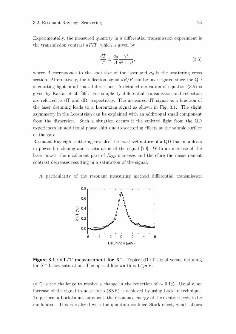
Experimentally, the measured quantity in a differential transmission experiment is
the transmission contrast dT/T , which is given by
dT
T∝ σ0
A
γ2
δ2 + γ2, (3.5)
where A corresponds to the spot size of the laser and σ0 is the scattering cross
section. Alternatively, the reflection signal dR/R can be investigated since the QD
is emitting light in all spatial directions. A detailed derivation of equation (3.5) is
given by Karrai et al. [69]. For simplicity differential transmission and reflection
are referred as dT and dR, respectively. The measured dT signal as a function of
the laser detuning leads to a Lorentzian signal as shown in Fig. 3.1. The slight
asymmetry in the Lorentzian can be explained with an additional small component
from the dispersion. Such a situation occurs if the emitted light from the QD
experiences an additional phase shift due to scattering effects at the sample surface
or the gate.
Resonant Rayleigh scattering revealed the two-level nature of a QD that manifests
in power broadening and a saturation of the signal [70]. With an increase of the
laser power, the incoherent part of EQD increases and therefore the measurement
contrast decreases resulting in a saturation of the signal.
A particularity of the resonant measuring method differential transmission
-6 -4 -2 0 2 4 6
0.0
0.2
0.4
0.6
0.8
dT
/T (
%)
Detuning (eV)
Figure 3.1.: dT/T measurement for X−. Typical dT/T signal versus detuningfor X− below saturation. The optical line width is 1.7µeV.
(dT) is the challenge to resolve a change in the reflection of ∼ 0.1%. Usually, an
increase of the signal to noise ratio (SNR) is achieved by using Lock-In technique.
To perform a Lock-In measurement, the resonance energy of the exciton needs to be
modulated. This is realized with the quantum confined Stark effect, which allows

24 Experimental Methods
to control the exciton transition energy via the gate voltage (see chapter 2.1.4).
To resolve the true line shape of the resonance, a square wave modulation of
Vpp = 100mV, which is an order of magnitude larger than the line width of
the resonance, is applied to the gate. Therefore two replica of the resonance at
V− = Vr− 1/2Vpp and V+ = Vr + 1/2Vpp can be observed in the measured spectrum.
In a Lock-In detection only the first Fourier component of the modulation frequency
is integrated and all other frequencies are filtered out. Therefore a higher SNR can
be achieved [31, 71].
3.3. Resonance Fluorescence
An alternative approach to perform resonant spectroscopy is to measure di-
rectly the response of the QD to the incident laser field, which corresponds to
〈| EQD(xdet) |2〉 in equation 3.1. The main difficulty is to achieve a sufficient
suppression of the laser such that the resonance fluorescence photons (RF) from
the QD are not overwhelmed by the laser background. The approach by Muller
et al. [72] relies on a spatial filtering of the resonant laser. Alternatively, a polar-
ization suppression of the laser by a factor of 106 allows for measuring resonance
fluorescence [73, 74]. Experimentally, this is realized by operating the microscope
in a dark-field configuration [75]. A linear polarizer that is perpendicular to the
incoming linearly polarized laser field is placed in front of the collection fiber. Sub-
sequently the RF photons are sent to an avalanche photodiode (APD). In contrast
to a dT measurement where the polarization of the signal is given by the laser, only
the photons that have a polarization component orthogonal to the excitation laser
are collected in RF measurements. Typically 103 − 106 counts/sec. are detected
from a single QD.
3.4. Pump Probe Measuring Methods
To explore the electron nuclear spin system with increasing transverse magnetic
field in chapter 4, it would be ideal to directly observe the dynamics of the electron
and nuclear spins. However, only the electron spin is directly accessible with current
measurement techniques. In contrast, nuclear spin polarization can only indirectly
be measured via the electron spin. This is possible due to the hyperfine interaction
that generates an energy shift (Overhauser shift ∆Eos) on the electron spin levels
which is proportional to the nuclear spin polarization. In this section we describe
a method to efficiently polarize nuclear spins and optically measure the magnitude
of nuclear spin polarization. Furthermore, two different pump probe measuring
methods are developed to access ∆Eos with resonant spectroscopy.

3.4. Pump Probe Measuring Methods 25
3.4.1. Optical detection of Nuclear Spin Polarization
There exist several methods to polarize nuclear spins in an InGaAs QD [66, 76, 77].
Most of them relay on the scalar form Se · I of the hyperfine interaction that con-
serves the total spin and the energy. By the relaxation of an electron spin via this
interaction, the spin angular momentum is transferred to a nuclear spin in the
so-called flip-flop process. Therefore, a large electron spin polarization obviously
helps to create significant nuclear spin polarization. Due to the selection rules
in a QD, which correlate the electron spin states with the light polarization, a
large electron spin polarization can be achieved by optical means. Since a sizable
nuclear spin polarization at Bx = 0 is required for the investigation of nuclear spin
dynamics in a transverse magnetic field Bx, we polarize nuclear spins by exciting
the QD into one of its excited p-shell states [66].
To guarantee a sizable nuclear spin polarization a single electron spin has to be
s- s+
ΔEOS
p-shell
s-shell s+
-100 0 1000
20000
40000
s+/s
+
s+/s
-
PLE
count
rate
(cts
/0.2
s)
Detuning (eV)
EOS
=18eV
(a) (b)
Figure 3.2.: Optical detection of nuclear spin polarization in X+. (a) Nu-clear spin polarization is achieved by resonantly pumping a single QD to one ofits excited states in the p-shell with a circularly polarized laser (e.g. σ+, green ar-row). Subsequently the emitted co- and cross- polarized photons are detected. (b)PLE spectra of X+ in zero magnetic field measured under co-polarized (σ+/σ+) andcross- polarized (σ+/σ−) excitation/detection configuration. The energy splitting∆Eos is induced by the Overhauser field.
either in the ground or excited state of the exciton, which is only fulfilled in a
charged QD. Additionally, we would like to monitor the electron spin polarization
via the polarization of the fluorescence, therefore the electron spin has to be in the
excited state. Out of these reasons we will focus our studies on the X+ state. A
schematic drawing of the X+ energy diagram is shown in Fig. 3.2 (b). The QD is
excited into the p-shell with a σ+ polarized laser. The Subsequent relaxation to
the s-shell takes place within picosecond timescales. The relaxation occurs due to a
combination of phonon-mediated relaxation and co-tunneling through the electron

26 Experimental Methods
reservoir. Finally the X+ state recombines to |⇓> (|⇑>) under the emission of a σ+
(σ−) polarized photon. These photons can be analyzed with a spectrometer. The
polarization configuration of the p-shell laser and the emitted photons is denoted
(σα/σβ) where σα is the excitation polarization and σβ represents the detection
polarization. Due to nuclear spin polarization an energy shift between |⇓⇑↓>and |⇑⇓↑> occurs. This so-called Overhauser shift ∆Eos is proportional to the
magnitude of the nuclear spin polarization in z-direction and can be measured by
separately analyzing the co- and cross- polarized emitted photons. Such a polariza-
tion sensitive detection method allows for a high spectral resolution up to 4µeV. For
all measurements the p-shell state was excited to saturation, which results in a high
polarization preservation. The polarization preservation can be quantified with the
degree of circular polarization which is defined as ρ+ = (I+− I+)/(I+ + I−), where
Ix is the PLE intensity in the (σ+, σx) polarization configuration. Experimentally,
a polarization preservation of up to ρ+ ∼ 80% can be measured.
The emitted PLE photons as a function of the energy detuning are shown for co-
and cross- polarized detection with respect to the excitation polarization in Fig. 3.2
(a). Clearly a high degree of polarization preservation is exhibited. The energy shift
of ∆EOS = 18µeV between the two polarization configurations corresponds to an
effective magnetic field experienced by the electron of Beff = ~ωeOS/geµB ∼ 500mT.
In summary, resonant excitation into the p-shell allows to polarize nuclear spins. In
order to measure the nuclear spin polarization the energy splitting of co- and cross-
polarized detection is extracted. Additionally, in X+ the electron spin polarization
can be measured determining the polarization of the emitted photons.
To achieve a higher spectral resolution for measuring nuclear spin polarization
compared to a spectrometer and to have a coherent measuring method to directly
investigate the optical transitions, resonant spectroscopy techniques in combination
with p-shell excitation were investigated. In this case the limiting factors for the
resolution are given by the optical line width that is determined by the homogeneous
broadening and the inhomogeneous broadening that arises from charge fluctuations
and distortions of the optical line shape.
3.4.2. Pump Probe Method with Resonant Rayleigh Scattering
One possibility to access the Overhauser shift resonantly is to combine the p-shell
pumping with resonant Rayleigh scattering, namely dR, which is described in
section 3.2.
We performed a dR measurement on X+ for different p-shell laser powers. The
results of this measurements are shown in Fig. 3.3 (black). Obviously, there is an
ideal PLE laser power of 12µW to achieve the largest reflection contrast. The signal

3.4. Pump Probe Measuring Methods 27
strength in resonant absorption measurements, like dR, is strongly dependent on
the population of the ground state of the optical transition [15, 78]. Only with a
sizable population of the ground state, a dR signal can be measured. Since the
ground state of the X+ consists of a single hole inside the QD, the PLE laser is
populating the QD with holes which is explained in detail in chapter 2. For weaker
PLE laser power than 12µW the reflection contrast is smaller due to reduced
population of the X+ ground state. A larger PLE laser power than 12µW results
in a population of excited states of X+. Therefore the single hole population inside
the QD is reduced, which leads to a smaller reflection contrast.
To investigate nuclear spin polarization in a transverse magnetic field (see chap-
1 1 0 1 0 00 . 0 3 50 . 0 4 00 . 0 4 50 . 0 5 00 . 0 5 50 . 0 6 00 . 0 6 5
L a s e r p o w e r ( µW )
Refle
ction
contr
ast (%
)
0
5
1 0
1 5
2 0
∆EOS (µeV)
Figure 3.3.: Comparison between dR and ∆ EOS. Reflection contrast (black)and ∆EOS (blue) as a function of PLE laser power.
ter 4) we are interested in a large Overhauser shift ∆Eos in addition to a sizable
reflection contrast. A comparison of the reflection contrast (black) and ∆Eos (blue)
as a function of the PLE laser power is shown in Fig. 3.3. Sizable nuclear spin
polarization of ∆Eos = 19µeV can only be achieved for a large PLE laser power of
several 100µW, where the reflection contrast is small.
One possibility is to choose the p-shell laser power such that a sizable reflection
contrast is reached at the cost of a reduced nuclear spin polarization. Another
approach is to combine the large Overhauser shift with a sizable reflection contrast
in a pulsed pump probe technique. While nuclear spins are polarized in the pump
sequence, a reduced p-shell laser power enables a sizable reflection contrast for the
resonant measurements in the probe sequence. To polarize nuclear spins, a p-shell
laser power of several hundred µW is needed. In order to perturb the system as
little as possible, the dR measurements take place with an additional weak p-shell
laser that is needed to charge the QD with a single hole. The probe signal depends
dramatically on the time constants of the experiment. If the measurement time

28 Experimental Methods
1 10 100
0
2
4
6
8
10
decay
=66ms
E
os(
eV
)
Twait
(ms)
0.1 1 10
0
2
4
6
8
10
E
OS
(eV
)
Tpump
(ms)
buildup
=2ms
(c) (d)
shutter
sample
t
t
c
o
AO
M
c
o
shutt
er
Tpump Tprobe Twait
(a) (b)
Figure 3.4.: Nuclear spin dynamics measured with p-shell emission. (a)Setup for pump probe measurement. The p-shell excitation laser is pulsed withan AOM. The pump laser is blocked with a mechanical shutter in front of thespectrometer. (b) Pulse sequence for the pump probe experiment. A long pumppulse Tpump polarizes nuclear spins, after a waiting time Twait a short p-shell laser(Tprobe) is needed to probe the sample. (c) ∆Eos is measured as a function ofTpump. An exponential fit (red) leads to a buildup time of nuclear spin polarizationτbuildup =2ms. (d) ∆Eos is measured as a function of Twait. An exponential fit (red)leads to a decay time of nuclear spin polarization τdecay =66ms.
(Tprobe) is larger than the decay time of nuclear spins (τdecay), ∆Eos is vanishes and
only one resonance is measured with a linearly polarized probe laser. In the case of
Tprobe < τdecay the Overhauser splitting can be determined with the energy splitting
between the two circularly polarized resonances. Hence this technique allows access
to the nuclear spin decay time by varying Tprobe.
In all following experiments we rely on the detection of the maximal Overhauser
shift. Therefore the time constants for build up and decay of nuclear spin polariza-
tion in X+ have to be determined. We realized this by a pump probe experiment
based on PLE as follows. In order to achieve well defined pump and probe pulses,
the cw laser amplitude is modulated with an AOM. Furthermore a mechanical
shutter is used to block the pump pulses while allowing the probe pulses to reach
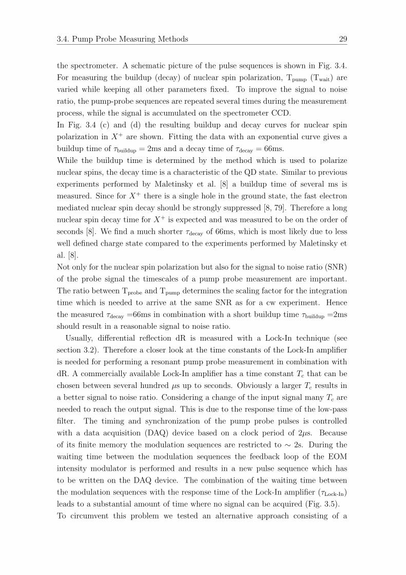
3.4. Pump Probe Measuring Methods 29
the spectrometer. A schematic picture of the pulse sequences is shown in Fig. 3.4.
For measuring the buildup (decay) of nuclear spin polarization, Tpump (Twait) are
varied while keeping all other parameters fixed. To improve the signal to noise
ratio, the pump-probe sequences are repeated several times during the measurement
process, while the signal is accumulated on the spectrometer CCD.
In Fig. 3.4 (c) and (d) the resulting buildup and decay curves for nuclear spin
polarization in X+ are shown. Fitting the data with an exponential curve gives a
buildup time of τbuildup = 2ms and a decay time of τdecay = 66ms.
While the buildup time is determined by the method which is used to polarize
nuclear spins, the decay time is a characteristic of the QD state. Similar to previous
experiments performed by Maletinsky et al. [8] a buildup time of several ms is
measured. Since for X+ there is a single hole in the ground state, the fast electron
mediated nuclear spin decay should be strongly suppressed [8, 79]. Therefore a long
nuclear spin decay time for X+ is expected and was measured to be on the order of
seconds [8]. We find a much shorter τdecay of 66ms, which is most likely due to less
well defined charge state compared to the experiments performed by Maletinsky et
al. [8].
Not only for the nuclear spin polarization but also for the signal to noise ratio (SNR)
of the probe signal the timescales of a pump probe measurement are important.
The ratio between Tprobe and Tpump determines the scaling factor for the integration
time which is needed to arrive at the same SNR as for a cw experiment. Hence
the measured τdecay =66ms in combination with a short buildup time τbuildup =2ms
should result in a reasonable signal to noise ratio.
Usually, differential reflection dR is measured with a Lock-In technique (see
section 3.2). Therefore a closer look at the time constants of the Lock-In amplifier
is needed for performing a resonant pump probe measurement in combination with
dR. A commercially available Lock-In amplifier has a time constant Tc that can be
chosen between several hundred µs up to seconds. Obviously a larger Tc results in
a better signal to noise ratio. Considering a change of the input signal many Tc are
needed to reach the output signal. This is due to the response time of the low-pass
filter. The timing and synchronization of the pump probe pulses is controlled
with a data acquisition (DAQ) device based on a clock period of 2µs. Because
of its finite memory the modulation sequences are restricted to ∼ 2s. During the
waiting time between the modulation sequences the feedback loop of the EOM
intensity modulator is performed and results in a new pulse sequence which has
to be written on the DAQ device. The combination of the waiting time between
the modulation sequences with the response time of the Lock-In amplifier (τLock-In)
leads to a substantial amount of time where no signal can be acquired (Fig. 3.5).
To circumvent this problem we tested an alternative approach consisting of a

30 Experimental Methods
0 1 2 30
1
0 . 05 . 0 x 1 0 - 6
1 . 0 x 1 0 - 5
1 . 5 x 1 0 - 5
01 0 02 0 03 0 0
0 1 2 3
Volta
ge (V
)
T i m e ( s )
m o d u l a t i o ns i g n a lτL o c k - I n
dR (1
E-8A
) ( b )
( c )
Ωpu
mp (µ
W) ( a )
Figure 3.5.: Measurement scheme for pump probe with dR. (a) Measure-ment of the pump laser power Ωpump versus time. The gap between the modulationsequences arises from writing the sequence on the DAQ device memory. (b) Cor-responding dR signal from Lock-In amplifier versus time. The strong pump laserbetween the modulation sequences leads to an increase of the dR signal. (c) Digitalsignal to be multiplied with Lock-in signal. To avoid memory effects the modulationof the dR signal is shifted by τLock-In.
software based Lock-In amplifier, which is implemented directly on the DAQ
device. With this method a synchronization of the Lock-In amplifier with the
pump probe pulses is possible such that the response time of the Lock-In amplifier
can be reduced. To compare the commercially available Lock-In amplifier from
Signal Recovery (SR) with the software based Lock-In amplifier, a cw experiment
was performed. The result is shown in Fig. 3.6. For the software based Lock-In
amplifier a decrease of the signal to noise ratio by a factor of ten is exhibited, which
is caused by the finite bandwidth of the used digital to analog converter on the
DAQ device. Even though a faster response time can be reached with a Lock-In
amplifier implemented on the DAQ device compared to the SR Lock-In amplifier,
the combination with the strongly reduced signal to noise ratio will not result in
a better performance for the pump probe experiment. Therefore the pump probe
experiments were realized with a commercially available Lock-In amplifier, taking

3.4. Pump Probe Measuring Methods 31
- 0 . 1 0 - 0 . 0 8 - 0 . 0 6 - 0 . 0 4- 5 . 0 x 1 0 - 5
0 . 0
5 . 0 x 1 0 - 5
dR (1
E-8A
)
G a t e V o l t a g e ( V )
D A Q c a r d S R L o c k - I n
Figure 3.6.: dR measurement with software based Lock-In amplifier. dRmeasurements as a function of gate voltage performed with a SR Lock-In amplifier(black) and a software based Lock-In amplifier (DAQ device) (red).
into account the slower response time compared to a Lock-In amplifier which is
based on the DAQ device.
For a first attempt at pump probe measurement with dR only the σ+ polarized
p-shell laser is pulsed while the resonant laser and a hole generating weak PL laser
is continuously on. During the entire measuring process, the gate is modulated for
the Lock-In detection (see Fig. (b)). In this experiment a fiber based EOM intensity
modulator served as a fast switch of the p-shell laser intensity. Besides the faster
rise time compared to an AOM, the fiber based intensity modulator has a larger
throughput. The intensity modulation is achieved with two EOMs that are forming
a Mach-Zehnder interferometer. By applying a voltage to the EOM the phase of the
light in one interferometer arm can be shifted with respect to the other. If the light
after recombination is out of phase a destructive interference is observed, resulting
in a reduced intensity. Unfortunately the voltage needed to apply to the EOM
for achieving a maximal suppression is drifting due to temperature fluctuations.
Either the environmental temperature or the heating of the device with a strong
pump laser can lead to temperature changes inside the intensity modulator. These
changes are rather slow therefore the voltage needed for a maximal suppression can
be stabilized with a control loop feedback mechanism (PID).
Similar to the co- and cross- circularly polarized probing performed in non-resonant
measurements, we compare σ+ and σ− resonant absorption. In Fig. 3.7 (a) dR
signal for both polarizations is plotted as a function of the laser detuning. From
top to bottom the measuring time between the pump pulses which is indicated with
Twait is decreased. Clearly, there is an observable energy shift up to 5µeV between
σ+/σ+ and σ+/σ−. Additionally, the asymmetry increases as the ratio between
Tpump and Twait increases which can be explained as follows. The consequence

32 Experimental Methods
-10 -5 0 5
-0.1
0.0
0.1
-0.1
0.0
0.1
0.2
-0.1
0.0
0.1
0.2
0.3
0.4
-10 -5 0 5
dR
(V
)
Detuning (eV)
dR
(V
)
Tpump
=10ms,
Twait
=3ms
Tpump
=10ms,
Twait
=10ms
Tpump
=10ms,
Twait
=5ms
+/
+
+/
-
dR
(V
)
- +
ΔEOS
z
z
z
p-shell
s-shell +
Gain
(a)
(c)
t
t
c
o
EO
M
off
resonant
on
gate
Tpump Twait
(b)
Figure 3.7.: Pump probe measurement with dR. (a) Pump Probe measure-ments of the Overhauser shift for different polarizations of the resonant laser. DRsignal versus detuning for a resonant σ+ polarized laser is shown in black, while for aresonant σ− polarized laser it is shown in red. The waiting time Twait and thereforethe measurement time is decreasing from top to bottom. (b) Measurement scheme.The pump laser is pulsed with an EOM, while the resonant laser and a weak PLlaser (to generate the hole for X+) is continuously on. Gate voltage is modulatedduring the measurement process and even on resonance during Tpump. (c) Energylevel diagram for X+. The σ+ pump laser polarizes nuclear spins by exciting to thep-shell (shown in green). Resonant measurements can be performed with σ+ (redarrow) or σ− (blue arrow). A large population of |⇓⇑↓> by the pump laser leads togain (indicated with dotted orange arrow).
of a strong p-shell laser is a large population of the |⇓⇑↓> state which leads
to stimulated emission (gain) in a dR measurement (Fig. 3.7 (c)). Therefore a
negative dR signal can be observed for a σ+ polarized resonant laser. Especially
the dependence on the ratio between Tpump and Twait can be understood by the
fact that the large population in |⇓⇑↓> is increasingly dominating for shorter Twait,
leading to the observed stimulated emission. In order to extract the energy splitting
∆Eos between σ+ and σ− polarized resonant excitation, the gain process is avoided
by modulating the gate voltage away from the X+ resonance during the strong
pump pulse.

3.4. Pump Probe Measuring Methods 33
- 5 0 5 1 0 1 5- 0 . 0 20 . 0 00 . 0 20 . 0 40 . 0 6
0 . 0 0
0 . 0 5
0 . 1 0
0 . 0
0 . 1
0 . 2- 5 0 5 1 0 1 5
dR (V
)
D e t u n i n g ( µe V )
T p u m p = 1 2 m s ,T w a i t = 1 . 4 m s
T p u m p = 1 2 m s ,T w a i t = 0 . 7 m s
dR (V
)
( b )
( c )
T p u m p = 1 2 m s ,T w a i t = 3 . 5 m s
dR (V
)
( a )
Figure 3.8.: Pump probe measurement with dR for different Twait. dR sig-nal versus detuning for a linearly polarized resonant laser is shown . The waiting timeand therefore the measurement time is decreasing from top to bottom. (a)With awaiting time of 3.5ms, nuclear spin polarization is already decayed to ∆EOS=3.5µeV.(b), (c) A further decrease of the waiting time leads to ∆EOS=7µeV.
The high spectral resolution of dR compared to PLE allows to measure the
Overhauser shift directly in a linear basis. In Fig. 3.8 the dR signal as a function
of the laser detuning is shown for decreasing measurement time Twait between the
pump pulses from top to bottom. With the realization of a gate modulation away
from the X+ resonance during the strong pump laser, two separated resonances
with a Lorentzian dR signal can be measured for a linearly polarized probe laser.
The maximal nuclear spin polarization is reached for Twait = 1.4ms. Because of
the constant pump time Tpump the ratio between the measuring time and Tpump is
decreasing from top to bottom and thus the signal to noise ratio (SNR).
Such a short nuclear spin depolarization time is surprising, especially since previous
measurements exhibited a τdecay of 66ms. One reason for a shortened decay time
could be the influence of the weak PL laser or the probe laser which are continuously

34 Experimental Methods
on. For a better understanding a detailed study including a pulsed weak PL laser
and probe laser would be needed.
3.4.3. Pump probe Method with Resonance Fluorescence
Although a resonant measurement of the Overhauser shift can be realized with
a pump probe method based on dR, the need for a Lock-In technique leads to a
substantial amount of time when no signal can be acquired as discussed in the
previous section. Alternatively resonance fluorescence (RF), that is explained in
detail in section 3.3, can be used as a resonant measuring method. This has the
advantage that no Lock-In technique is needed and therefore a higher SNR in
a pump probe experiment should be achieved compared to dR. Switching from
resonant Rayleigh scattering to RF does not alter the experiment substantially, only
changing the polarization of the excitation laser is a much more time consuming
task for RF than for dR because of the alignment of the polarizer in order to achieve
a high polarization suppression.
In Fig. 3.9 (a) a scheme for the pump probe measurements with RF is shown.
Similar to the previous pump probe technique, the pump pulses are generated
with an EOM while a weak hole generating PL laser and the resonant laser
are continuously on. Especially during Tpump a suppression of the background
is difficult because the emitted PLE photons cannot be distinguished from RF
photons. Therefore only the photons between two pump pulses, during Twait are
detected. The resulting RF count rate for a σ− polarized pump laser and a linearly
polarized resonant laser as a function of the laser detuning is shown in Fig. 3.9 (b).
Compared to the measurement shown in Fig. 3.8 a reasonable signal to noise ratio
is achieved with less integration time.
To conclude, a resonant pump probe technique to measure nuclear spin po-
larization is realized with dR and RF. A comparison of these methods shows an
easier polarization control for dR which is contrasted by the improved signal to
noise ratio of RF measurements.
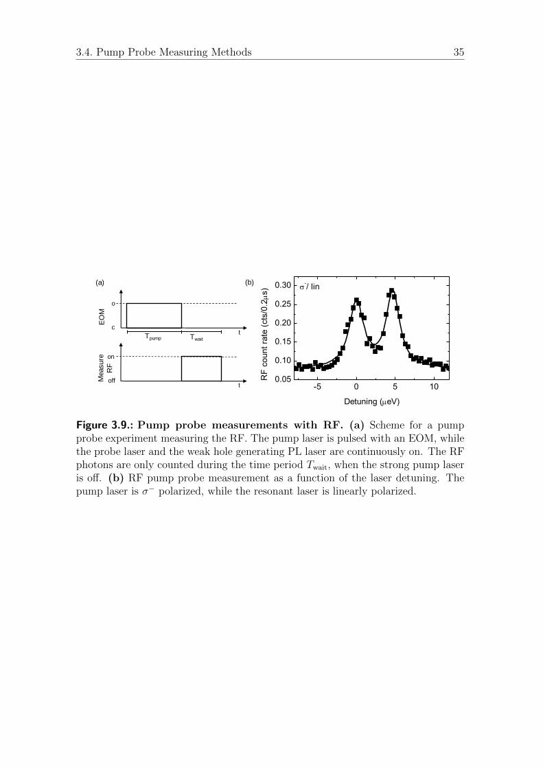
3.4. Pump Probe Measuring Methods 35
t
t
c
o
EO
M
off
on
Measure
RF
Tpump Twait
(a) (b)
-5 0 5 100.05
0.10
0.15
0.20
0.25
0.30 -/ lin
RF
count
rate
(cts
/0.2s)
Detuning (eV)
Figure 3.9.: Pump probe measurements with RF. (a) Scheme for a pumpprobe experiment measuring the RF. The pump laser is pulsed with an EOM, whilethe probe laser and the weak hole generating PL laser are continuously on. The RFphotons are only counted during the time period Twait, when the strong pump laseris off. (b) RF pump probe measurement as a function of the laser detuning. Thepump laser is σ− polarized, while the resonant laser is linearly polarized.


Nuclear Spin Polarization in Transverse Magnetic Fields 37
4. Nuclear Spin Polarization in
Transverse Magnetic Fields
We investigated nuclear spin polarization in individual self-assembled
InAs/GaAs quantum dots for different sample structures in transverse mag-
netic fields. Hanle depolarization curves are measured to explore nuclear
spin dynamics, leading to an anomalous Hanle curve with a broadening up
to 1T. Even though nuclear spin polarization is comparable for different
sample structures at zero magnetic field, the broadening of the anomalous
Hanle curve is substantially different. The critical field, at which the pho-
tocreated electron spin polarization breaks down, depends strongly on the
electron spin lifetime. For further investigation of direction and strength of
the Overhauser field causing the broadening of the Hanle curve, a resonant
measurement technique is applied.
4.1. Introduction
A phase transition is the transformation of a physical system from one state
to another, such as vaporization and condensation. These transitions manifest in
unconventional and unexpected physical behavior and do not only occur at finite
temperature. Even at zero temperature or ~ω > kBT quantum fluctuations (at
energy ~ω) are expected to lead to so-called quantum phase transitions. In order
to have experimental access to a quantum system, a coupling to the environment
is needed which leads to dissipation. Dissipative phase transitions can occur if an
environmental parameter is varied such as a magnetic field or an external coherent
source (e. g. a laser) [80–82]. Investigations on dissipative phase transitions (DPT)
are expected to lead to a deeper understanding of the unexpected physical behavior
of systems at low temperatures.
A model exhibiting first- and second- order DPT is the central spin system which
is externally driven and decays through interaction with a Markovian environ-
ment [83]. In its simplest form, a central spin system consists of a set of spin-
1/2 particles, uniformly coupled to a single spin-1/2. A possible experimental

38 Nuclear Spin Polarization in Transverse Magnetic Fields
implementation of such a system is a negatively charged InGaAs QD, where nuclear
spins represent the set of spin- 1/2 particles and the electron is the single spin-1/2
particle. Accordingly, the nuclear spin ensemble is expected to undergo phase
transitions. The behavior of the nuclear spin ensemble can be monitored via the
interaction between nuclear and electron spins. If a negatively charged InGaAs QD
is driven by a laser, it experiences spontaneous decay and therefore satisfies the
requirements of the theoretical model studied by Kessler et al. [83]. On the other
hand the model does not consider inhomogeneous hyperfine coupling, the electron
Zeeman splitting and the nuclear quadrupolar interactions [51, 52] in InGaAs QDs,
which raises the question to what extent an experimental observation of dissipative
phase transitions is possible in this system. Still, in recent experiments on InGaAs
QDs indications for a first order phase transition in the nuclear spin ensemble
were observed, including optical bistability as a function of a transverse magnetic
field Bx [20]. Therefore we want to further investigate the electron - nuclear spin
system under the influence of Bx with an increased spectral resolution to identify
discontinuities in the polarization of the nuclear spin ensemble. An abrupt change
in electron and nuclear spin polarization would signal a dissipative phase transitions
and lead to new insights into the electron nuclear spin system.
4.2. Hanle experiment
In a Hanle measurement, the dynamics of an electron spin in a transverse mag-
netic field Bx is determined by optical means. In the course of such an experiment
an exciton is created with a circularly polarized excitation laser. A schematic draw-
ing of the measurement geometry is shown in Fig. 4.1(a). Because of the selection
rules in a QD, the electron spin polarization S0 is optically defined along the z-axis
parallel to the Poynting vector of the excitation laser. In the case a finite magnetic
field Bx is applied, the optically generated electron spin undergoes Larmor preces-
sion around the x-axis at frequency Ωel = gelµBB/~ (see Fig. 4.1(b)). Due to the
fact that the projection of the electron spin onto the z-axis defines the degree of
circular polarization of the emitted photons, a depolarization of the PL light can
be observed as a function of Bx. This dependence allows to determine both, the
electron spin lifetime τs and the recombination time τ of the exciton [48].
The electron spin precession together with spin pumping, spin relaxation and re-
combination can be described with the following equation of motion for the spin
vector ~S :d~S
dt= ~Ωel × ~S −
~S
τs−~S − ~S0
τ. (4.1)
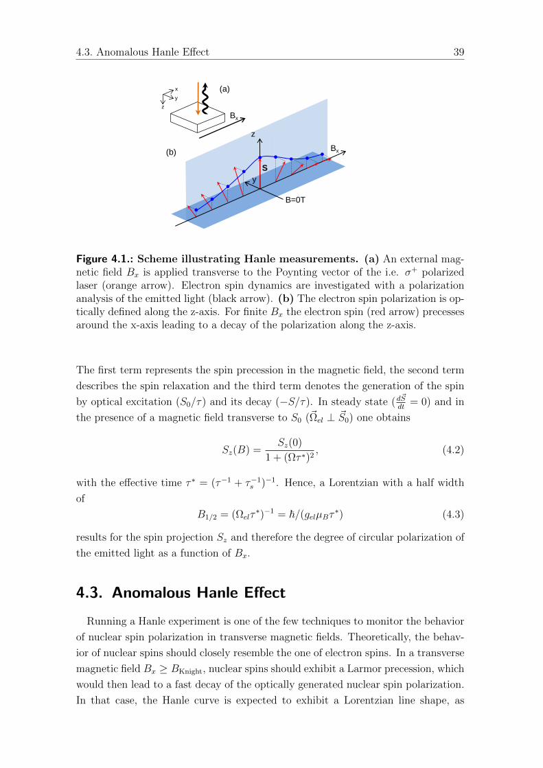
4.3. Anomalous Hanle Effect 39
B=0T
y
z
Bx
S
Bx
y
z
x
(a)
(b)
Figure 4.1.: Scheme illustrating Hanle measurements. (a) An external mag-netic field Bx is applied transverse to the Poynting vector of the i.e. σ+ polarizedlaser (orange arrow). Electron spin dynamics are investigated with a polarizationanalysis of the emitted light (black arrow). (b) The electron spin polarization is op-tically defined along the z-axis. For finite Bx the electron spin (red arrow) precessesaround the x-axis leading to a decay of the polarization along the z-axis.
The first term represents the spin precession in the magnetic field, the second term
describes the spin relaxation and the third term denotes the generation of the spin
by optical excitation (S0/τ) and its decay (−S/τ). In steady state (d~Sdt
= 0) and in
the presence of a magnetic field transverse to S0 (~Ωel ⊥ ~S0) one obtains
Sz(B) =Sz(0)
1 + (Ωτ ∗)2, (4.2)
with the effective time τ ∗ = (τ−1 + τ−1s )−1. Hence, a Lorentzian with a half width
of
B1/2 = (Ωelτ∗)−1 = ~/(gelµBτ ∗) (4.3)
results for the spin projection Sz and therefore the degree of circular polarization of
the emitted light as a function of Bx.
4.3. Anomalous Hanle Effect
Running a Hanle experiment is one of the few techniques to monitor the behavior
of nuclear spin polarization in transverse magnetic fields. Theoretically, the behav-
ior of nuclear spins should closely resemble the one of electron spins. In a transverse
magnetic field Bx ≥ BKnight, nuclear spins should exhibit a Larmor precession, which
would then lead to a fast decay of the optically generated nuclear spin polarization.
In that case, the Hanle curve is expected to exhibit a Lorentzian line shape, as

40 Nuclear Spin Polarization in Transverse Magnetic Fields
described by Eq. 4.3, with a FWHM of 30mT for a ge = 0.5 and an effective time
dominated by the trion radiation lifetime τ ∗ ∼ τ = 0.7ns.
A typical Hanle depolarization curve, measured according to section 3.4.1, is shown
in Fig. 4.2 (a). The most striking anomaly to the theoretical predictions is the 40
times broadening of the FWHM. This unexpected broadening is termed anomalous
Hanle effect. In addition, the Hanle curve exhibits a large hysteresis of 0.5T. The
degree of circular polarization is continuously decreasing for magnetic fields up to
0.5T, where it reaches a minimum value of 50%. For larger magnetic fields the de-
gree of circular polarization increases again until a sudden drop down from 70% to
0% is observed at a critical magnetic field Bcrit = 1.1T. Similar results have been
presented in the detailed studies by Krebs et al. [20].
Together with the hysteresis, the broadening of the Hanle curve is a strong indication
for nuclear spin effects. By modulating σ+/σ− polarization at kHz frequency, an
optical polarization of nuclear spins can be prevented [8]. This effect was exploited
in an additional measurement. The resulting Hanle curve exhibited a narrowing.
Therefore we conclude that the nuclear spin polarization is the cause for the anoma-
lous broadening of the Hanle curve in InGaAs QD.
In addition to the PL circular depolarization data, the Overhauser shift can be ex-
tracted from the same experiment (Fig. 4.2 (b)). The results show a decrease of
nuclear spin polarization along the z-axis with Bx. At the same time a high degree
of PL circular polarization is measured (Fig. 4.2 (a)). This leads to the conclusion
that a nuclear spin polarization along the x-axis is very likely to compensate Bx
and prevents the electron spin from performing Larmor precession. The underlying
mechanism that could cause a rotation of the nuclear spin polarization from the z-
axis to the x-axis as a function of Bx is not fully understood. Such a situation could
result from a tilted effective magnetic field, that is stabilized along the z-axis by a
Bnucz due to nuclear quadrupolar interactions (QI) [20]. This is further supported
by the modest broadening of the Hanle curves measured on strain-free droplet QDs,
which do not exhibit QI [84]. Should there exist a tilted effective magnetic field, a
finite nuclear spin polarization along the z-axis must be observed up to Bcrit. The
data shown in Fig. 4.2 (b) do not allow to draw a clear conclusion in this respect.
To verify the existence of such a nuclear polarization component an experimental
technique with increased resolution needs to be applied.

4.4. Hanle measurements for samples with different electron spin lifetimes 41
-1.5 -1.0 -0.5 0.0 0.5 1.0
0.0
0.2
0.4
0.6
0.8
1.0
PL c
ircula
r pola
rization
Bx(T)
(a)
(b)
-1.5 -1.0 -0.5 0.0 0.5 1.0
0
5
10
E
(eV
)
Bx(T)
Figure 4.2.: Anomalous Hanle effect. (a) Hanle depolarization curve as a func-tion of the transverse magnetic fieldBx measured on a 25nm tunneling barrier sample(sample B). Arrows indicate field sweep direction. (b) Corresponding energy shift∆EOS between co- and cross- polarized detection as a function of Bx.
4.4. Hanle measurements for samples with different
electron spin lifetimes
In the previous section, the Hanle effect was studied for a sample with 25nm
tunnel barrier (sample B) and exhibits a spectacular Hanle curve broadening
because of nuclear spin polarization. For a further investigation of the connection
between nuclear spin polarization and Bcrit we measured samples with different
electron spin lifetimes. This is of particular interest since the decay of nuclear spins
can be caused by a randomization of the electron spin [5]. Therefore the increased
electron spin lifetime of a 35nm tunnel barrier sample (sample A) compared to a
25nm tunnel barrier sample (sample B) should result in a better preservation of
nuclear spin polarization which could lead to an increased magnitude of nuclear
spin polarization and to even larger values for Bcrit.
In this section, we present a series of Hanle measurements for different values of
nuclear spin polarization at Bx = 0 on the same QD to verify to what extent this

42 Nuclear Spin Polarization in Transverse Magnetic Fields
-1.0 -0.5 0.0 0.5 1.0
0.0
0.2
0.4
0.6
0.8
1.0
PL c
ircula
r pola
rization
Bx(T)
-1.0 -0.5 0.0 0.5 1.0
0
5
10
15
20
E
(eV
)
Bx(T)
B
B (a)
(b)
0.3 0.4 0.5 0.6 0.70
5
10
15
20
E
OS(
eV
)
Bcrit
(T)
(c)
Figure 4.3.: Hanle measurements for different nuclear spin polarizations.(a) Hanle depolarization curves for a QD on sample B with a 25nm tunnelingbarrier. Arrows indicate field sweep direction. (b) Corresponding energy splitting∆E between co- and cross- polarized detection. (c) Extracted Bcrit for different∆Eos at Bx = 0T.
parameter influences the broadening of the Hanle curve Bcrit. Subsequently, the
width of the Hanle curve will be compared for the two different sample structures
A and B.
A typical Hanle depolarization curve for sample B is shown in Fig. 4.3(a). Similar
to the measurements in the previous section, an increased broadening up to
Bcrit = 0.75T and a hysteresis can be observed. The corresponding nuclear spin
polarization in z-direction is extracted and plotted as a function of Bx (Fig. 4.3(b)).
At Bx = 0T a large Overhauser splitting of ∆Eos = 20µeV is obtained that
decreases continuously as a function of Bx until Bx = Bcrit. At this point an abrupt
drop down to zero is observed. To further investigate the broadening of the Hanle
curve for different initial values of ∆Eos at Bx =0T, we varied the laser power for
the p-shell pumping. The results clearly show an increase of Bcrit as a function of
∆Eos at Bx =0T (Fig. 4.3(c)).

4.4. Hanle measurements for samples with different electron spin lifetimes 43
To compare the two sample structures A and B with different electron spin
lifetimes, we first investigated the magnitude of the nuclear spin polarization at
Bx = 0. Testing several p-shell resonances for different QDs did not reveal any
significant difference for the maximal ∆Eos. This result can be explained in two
possible ways. Either the dominant depolarization mechanism is not smaller for the
longer electron spin lifetime or the p-shell pumping is less effective for the longer
electron spin lifetime. Since p-shell pumping relies on a well defined X+ state to
polarize nuclear spins, we contrasted the fluorescence spectrum from sample A with
the one from sample B (Fig. 4.4). For sample B, a very clean spectrum is measured,
where as sample A can obviously be excited to a multitude of states. This is due
to the fact that a longer electron spin lifetime leads to less well defined charge
states [62, 85]. Therefore a smaller nuclear spin polarization rate for sample A is
expected. Hence a longer electron spin lifetime does not result in a larger ∆Eos at
Bx = 0.
According to previous experiments the broadening of the Hanle curve scales with
(a)
(b)
960 962 964 966 968 9700
5000
10000
15000
20000
X+
PLE
count
rate
(cts
/0.5
sec)
Wavelength (nm)
B
952 954 956 958 960 962
0
5000
10000
15000
20000
PLE
count
rate
(cts
/0.5
sec)
X+
Wavelength (nm)
A
Figure 4.4.: Emission at the s-shell.P-shell excitation at saturation for sampleA with a 35nm tunneling barrier (a) and sample B with a 25nm tunneling barrier(b).
∆Eos at Bx = 0 for the same QD on the same sample (Fig. 4.3 (c)). To investigate

44 Nuclear Spin Polarization in Transverse Magnetic Fields
-1.5 -1.0 -0.5 0.0 0.5 1.0
0.0
0.2
0.4
0.6
0.8
1.0
PL c
ircula
r pola
rization
Bx(T)
-1.5 -1.0 -0.5 0.0 0.5 1.0
0
5
10
E
(eV
)
Bx(T)
-0.4 -0.2 0.0 0.2 0.4
0.0
0.2
0.4
0.6
0.8
1.0
PL c
ircula
r pola
rization
Bx(T)
A B
B
(a) (b)
(c) (d)
-0.4 -0.2 0.0 0.2 0.4
0
5
10
E
OS (eV
)
B
x(T)
A
Figure 4.5.: Hanle measurements for different sample structures. (a-b)Hanle depolarization curves for a QD on sample B with a 25nm tunneling barrierand a QD on sample A with a 35nm tunneling barrier. Arrows indicate field sweepdirection. (c-d) Corresponding energy splitting ∆E between co- and cross- polarizeddetection.
the influence of the electron spin lifetime on Bcrit we performed Hanle measurements
with similar values for ∆Eos at Bx = 0T in sample A and B. In Fig. 4.5 (a-b) typical
Hanle depolarization curves for the two different sample structures A and B are
shown. The most striking difference is the broadening of Hanle curve which is 0.4T
for sample A and 1.5T for sample B. A second difference is the hysteresis, which
reaches up to 0.7T in sample B and vanishes completely for sample A. The third
difference concerns the line shape. All Hanle curves in sample A show a smooth
line shape while for sample B abrupt jumps appear at Bx = Bcrit. This leads to the
conclusion that the nuclear spin polarization at zero magnetic field is not the only
parameter that influences the broadening of the anomalous Hanle curve. In contrast
to what was observed in GaAs droplet dots [84] the magnitude of the nuclear spin
polarization increases during the Hanle measurements and the mechanism which
rotates nuclear spin polarization from the z-axis to the x-axis is unknown. This
makes direct conclusions for the impact of nuclear spin polarization along the

4.5. Resonant measurements on a 35nm tunnel barrier sample 45
z-axis on Bcrit very difficult. Further studies are necessary to fully understand the
increasing nuclear spin polarization along the x-axis in a Hanle measurement.
In addition to the Hanle curve we investigate nuclear spin polarization in z-direction
with the energy splitting ∆Eos between co- and cross- polarized detection of the
emitted light (Fig. 4.5 (c)-(d)). For both samples ∆Eos continuously decreases from
12µeV at Bx = 0 to around zero at 0.4T. While for sample A 0.4T corresponds to
Bcrit, sample B exhibits a broadening of the Hanle curve up to 1.1T. For sample B
the measured ∆Eos = 2µeV in the region between 0.4T and 1.1T is at the resolution
limit for a non-resonant measurement method (see section 3.4.1). Therefore it
is very difficult to claim a persistence of a small nuclear magnetic field along
the z-axis up to Bcrit. In order to achieve a better understanding of the nuclear
spin polarization dynamics in a transverse magnetic field, an increased spectral
resolution is needed.
A valuable alternative to the analysis of the QD fluorescence with a spectrometer
is the resonant excitation of the QD, which was performed with resonance fluores-
cence (RF). A resonant measurement offers an at least four times higher spectral
resolution which is limited due to the optical line width (see chapter 2). In contrast
to non-resonant measurements, RF is an absorption experiment which allows for
a direct access of the optical transitions in the s-shell. With the determination of
the polarization and the energy difference of these transitions, information about
magnitude and direction of nuclear spin polarization is gained.
4.5. Resonant measurements on a 35nm tunnel
barrier sample
To prove that the outcome of the experiment can be reproduced by resonant
spectroscopy, we performed a pump probe measurement with RF on sample A with
a 35nm tunnel barrier. In former measurements a narrow Hanle curve with no
abrupt change in the polarization conservation was obtained. This means that for
the electron spin there is no complete compensation of the external field Bx caused
by the nuclear spin polarization, which can suddenly break down. Therefore we
would also expect a gradual change from the Overhauser splitting to the Zeeman
splitting for increasing Bx.
To study the dynamics of ∆Eos resonantly, a σ+ polarized pump laser is used and
the X+ state was resonantly probed with a weak diagonally polarized laser. At zero
magnetic field, two resonances are observed, which are energetically separated by
the Overhauser shift ∆E=10µeV (Fig. 4.6). With increasing magnetic field Bx a
decrease of ∆Eos is observed. As a result the two resonances merge at Bx = 0.1T.

46 Nuclear Spin Polarization in Transverse Magnetic Fields
0 . 1 2 0 . 1 4 0 . 1 60 . 2
0 . 4
0 . 6
0 . 8
1 . 0
1 . 2
1 . 4
1 T0 . 2 5 T0 . 2 T0 . 1 5 T0 . 1 T0 . 0 5 T0 T
RF co
unt ra
te (ct
s/0.2µ
s)
G a t e V o l t a g e ( V )
Figure 4.6.: RF measurements sample A. Resonant measurements for differentin-plane magnetic fields, performed on a 35nm tunneling barrier sample.
For Bx = 0.2T an evolution into two resolvable resonances is measured because of the
Zeeman splitting. Finally, four resonances can be observed for a large magnetic field
of Bx = 1T. This is due to the fact that in Voigt geometry (transverse magnetic field)
all four transitions of X+ are allowed and linearly polarized [78, 86, 87]. Similar to
non-resonant measurements on the same sample structure, a gradual decrease of the
Overhauser shift can be observed. From the smooth Hanle curve we expect no abrupt
change in the nuclear spin polarization. This is confirmed in resonant measurements.
Hence the resonant pump probe technique allows for investigations of nuclear spin
dynamics in transverse magnetic fields with an enhanced measurement resolution
compared to non-resonant measurements.
4.6. Resonant measurements on a 25nm tunnel
barrier sample
Hanle measurements on sample B with a 25nm tunnel barrier showed an anoma-
lous broadening of the Hanle curve. First, we would like to reproduce these features
which are the abrupt jumps from circular to linear polarization of the emitted
photons, hysteresis and a large value for Bcrit on the order of 1.5T. In a second
step we aim at further investigating the mechanism which rotates the nuclear spin

4.6. Resonant measurements on a 25nm tunnel barrier sample 47
polarization from the z- to the x-axis.
4.6.1. Gate properties
In order to ensure good charge screening, we rely on the diode structure and in
particular a well grounded back contact. Without the latter, the optically generated
charges get trapped and can result in a reduced frequency bandwidth and thus in
a large RC time constant. It turned out that the back gate of the sample to be
studied was difficult to contact. This is most certainly due to the degradation of the
sample material. Therefore special attention has to be paid to the contact quality.
To test the frequency bandwidth of the gate, we applied a square wave modulation
with a large amplitude such that the two Stark shifted resonances can be resolved
with a spectrometer (Fig. 4.7). By increasing the modulation frequency to 700Hz a
merging to one broad resonance is observed. This is a consequence of the reduced
frequency bandwidth and confirms an incomplete grounding of the back contact.
Therefore the charge screening in the sample structure is restricted.
Not only for a fast gate modulation a good charge screening is needed. Particu-
973.0 973.2 973.4 973.6
1000
2000
3000
counts
/0.5
s
Wavelenght (nm)
2Hz
200Hz
700Hz
Figure 4.7.: Gate modulation at different frequencies. PL counts versus wave-length for different gate modulation frequencies. At 2Hz there are two Stark shifted,well separated resonances observable. For a modulation frequency of 200Hz alreadya merging of the two resonances starts, which evolves at 700Hz to one broad reso-nance. This is due to the incomplete grounding of the back contact.
larly, a strong p-shell pump laser generates a lot of charge carriers in the sample.
Without a well grounded back contact, these charges are trapped and can lead
to fluctuations and a broadening of the resonances in the subsequent measuring
process. In a pump probe experiment performed on sample B, very broad optical
line widths were measured independent of the polarization of the pump laser. As a
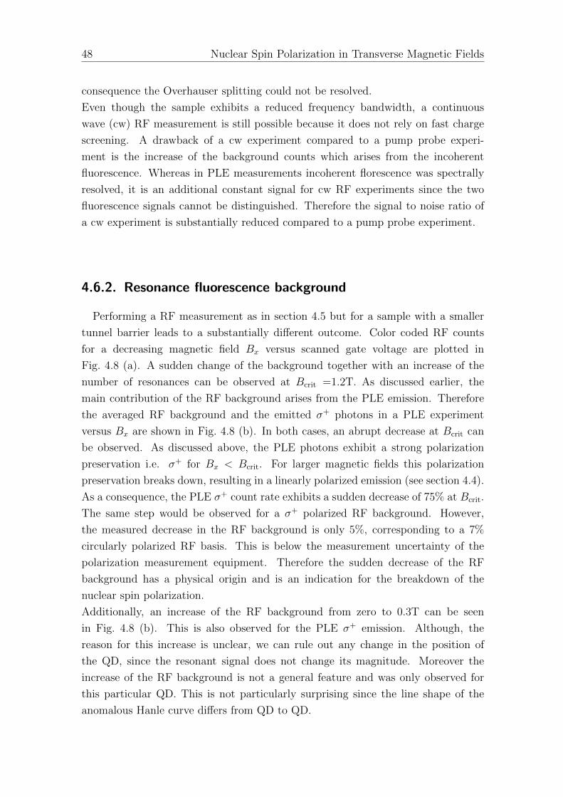
48 Nuclear Spin Polarization in Transverse Magnetic Fields
consequence the Overhauser splitting could not be resolved.
Even though the sample exhibits a reduced frequency bandwidth, a continuous
wave (cw) RF measurement is still possible because it does not rely on fast charge
screening. A drawback of a cw experiment compared to a pump probe experi-
ment is the increase of the background counts which arises from the incoherent
fluorescence. Whereas in PLE measurements incoherent florescence was spectrally
resolved, it is an additional constant signal for cw RF experiments since the two
fluorescence signals cannot be distinguished. Therefore the signal to noise ratio of
a cw experiment is substantially reduced compared to a pump probe experiment.
4.6.2. Resonance fluorescence background
Performing a RF measurement as in section 4.5 but for a sample with a smaller
tunnel barrier leads to a substantially different outcome. Color coded RF counts
for a decreasing magnetic field Bx versus scanned gate voltage are plotted in
Fig. 4.8 (a). A sudden change of the background together with an increase of the
number of resonances can be observed at Bcrit =1.2T. As discussed earlier, the
main contribution of the RF background arises from the PLE emission. Therefore
the averaged RF background and the emitted σ+ photons in a PLE experiment
versus Bx are shown in Fig. 4.8 (b). In both cases, an abrupt decrease at Bcrit can
be observed. As discussed above, the PLE photons exhibit a strong polarization
preservation i.e. σ+ for Bx < Bcrit. For larger magnetic fields this polarization
preservation breaks down, resulting in a linearly polarized emission (see section 4.4).
As a consequence, the PLE σ+ count rate exhibits a sudden decrease of 75% at Bcrit.
The same step would be observed for a σ+ polarized RF background. However,
the measured decrease in the RF background is only 5%, corresponding to a 7%
circularly polarized RF basis. This is below the measurement uncertainty of the
polarization measurement equipment. Therefore the sudden decrease of the RF
background has a physical origin and is an indication for the breakdown of the
nuclear spin polarization.
Additionally, an increase of the RF background from zero to 0.3T can be seen
in Fig. 4.8 (b). This is also observed for the PLE σ+ emission. Although, the
reason for this increase is unclear, we can rule out any change in the position of
the QD, since the resonant signal does not change its magnitude. Moreover the
increase of the RF background is not a general feature and was only observed for
this particular QD. This is not particularly surprising since the line shape of the
anomalous Hanle curve differs from QD to QD.

4.6. Resonant measurements on a 25nm tunnel barrier sample 49
-0.63 -0.62 -0.61 -0.60 -0.590.0
0.5
1.0
1.5
2.0
Gate voltage (V)
Bx (
T)
3.4E+04
3.8E+04
4.2E+04
4.5E+04
0.0 0.2 0.4 0.6 0.8 1.0 1.2 1.40
50
100
150
200
250
Bx(T)
PLE
+ c
ount
rate
(cts
/s)
32500
35000
37500
40000
42500 RF
backgro
und (c
ts/s
)
(a)
(b)
Figure 4.8.: CW RF measurements sample B. (a) RF measurements for de-creasing in-plane magnetic field Bx versus gate voltage. White lines are a guide tothe eye indicating the Zeeman splitting. Performed on a 25nm tunneling barriersample (B).(b) Averaged background from RF measurements (blue) as a functionof Bx in comparison with the emitted σ+ photons in a PLE experiment (black). Anabrupt jump at Bcrit is observable in both cases.
4.6.3. Extraction of the resonance positions
Not only the abrupt change in the RF background at Bcrit is an indication for the
breakdown of nuclear spin polarization but also the number of resonances before
and after Bcrit =1.2T. In contrast to PLE measurements, the increased spectral
resolution of the RF measurements allows to measure four resonances above Bcrit
for the first time. Line cuts below and above Bcrit of the measurements shown
in Fig. 4.8 (a) are plotted in Fig. 4.9 (a). Below Bcrit we observe a pair of split
resonances separated by the hole Zeeman splitting (|gh|µBBx). This observation
is fully consistent with the cancellation of Bx with an in-plane Overhauser field.
Above Bcrit the nuclear spin polarization breaks down, resulting in an additional
electron Zeeman splitting (|ge|µBBx) [20]. The expected fourth resonance lies just
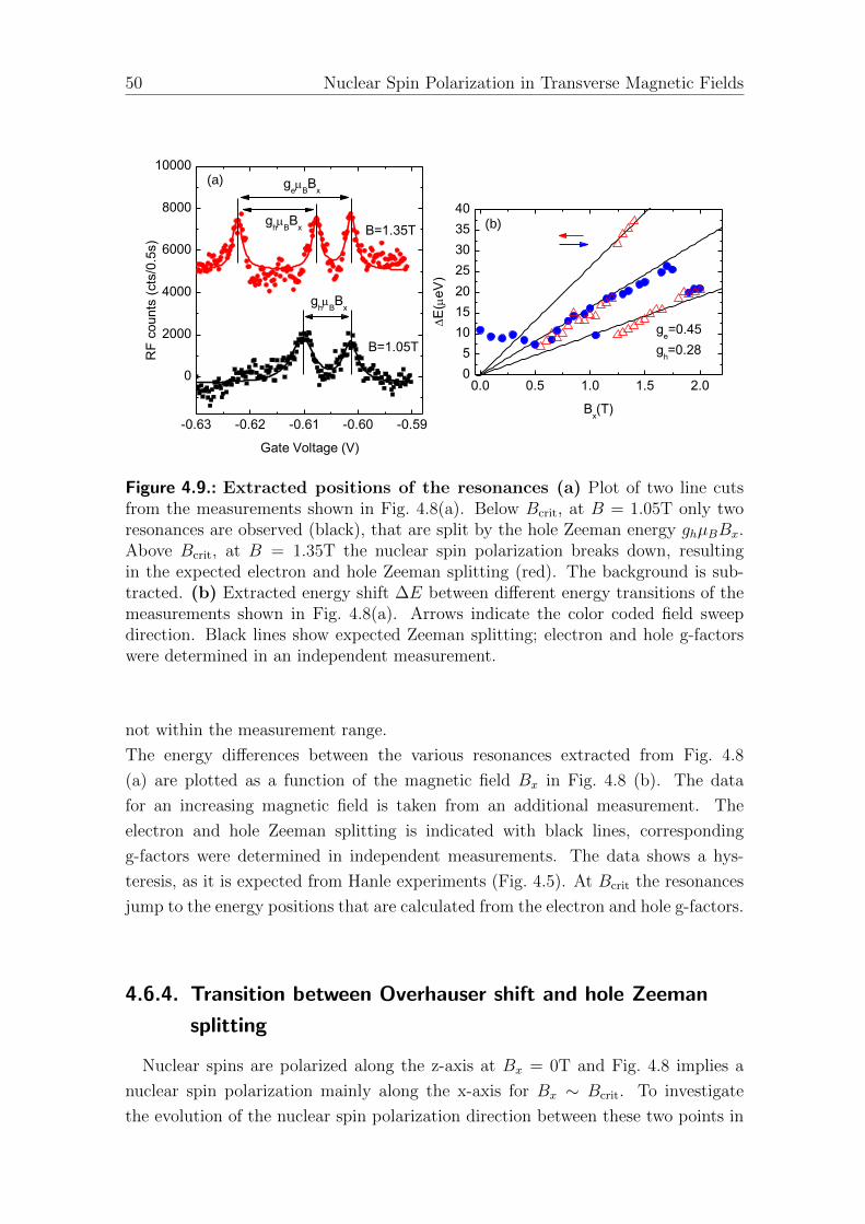
50 Nuclear Spin Polarization in Transverse Magnetic Fields
-0.63 -0.62 -0.61 -0.60 -0.59
0
2000
4000
6000
8000
10000
ge
BB
x
gh
BB
x
gh
BB
x
RF
counts
(cts
/0.5
s)
Gate Voltage (V)
B=1.05T
B=1.35T
(a)
(b)
0.0 0.5 1.0 1.5 2.00
5
10
15
20
25
30
35
40
E
(eV
)
Bx(T)
ge=0.45
gh=0.28
Figure 4.9.: Extracted positions of the resonances (a) Plot of two line cutsfrom the measurements shown in Fig. 4.8(a). Below Bcrit, at B = 1.05T only tworesonances are observed (black), that are split by the hole Zeeman energy ghµBBx.Above Bcrit, at B = 1.35T the nuclear spin polarization breaks down, resultingin the expected electron and hole Zeeman splitting (red). The background is sub-tracted. (b) Extracted energy shift ∆E between different energy transitions of themeasurements shown in Fig. 4.8(a). Arrows indicate the color coded field sweepdirection. Black lines show expected Zeeman splitting; electron and hole g-factorswere determined in an independent measurement.
not within the measurement range.
The energy differences between the various resonances extracted from Fig. 4.8
(a) are plotted as a function of the magnetic field Bx in Fig. 4.8 (b). The data
for an increasing magnetic field is taken from an additional measurement. The
electron and hole Zeeman splitting is indicated with black lines, corresponding
g-factors were determined in independent measurements. The data shows a hys-
teresis, as it is expected from Hanle experiments (Fig. 4.5). At Bcrit the resonances
jump to the energy positions that are calculated from the electron and hole g-factors.
4.6.4. Transition between Overhauser shift and hole Zeeman
splitting
Nuclear spins are polarized along the z-axis at Bx = 0T and Fig. 4.8 implies a
nuclear spin polarization mainly along the x-axis for Bx ∼ Bcrit. To investigate
the evolution of the nuclear spin polarization direction between these two points in

4.6. Resonant measurements on a 25nm tunnel barrier sample 51
(a)
(b)
-0.60 -0.59 -0.580.0
0.2
0.4
0.6
0.8
1.0
1.2
1.4
Gate voltage (V)
Bx(T
)
-5 0 5 10 15
0
1000
2000
3000
4000
5000
RF
count
rate
(cts
/sec)
Detuning (eV)
1T
0.45T
0.1T
0T
Figure 4.10.: Transition between Overhauser shift and Zeeman splitting.(a) Resonant measurements for increasing in-plane magnetic fields below Bcrit. Res-onant excitation laser is vertically polarized with respect to the QD axes. (b) Linecuts for selected magnetic fields Bx.
more detail, a resonant RF measurement was performed in an increasing magnetic
field below Bcrit and with a smaller step size of Bx = 0.025T. The result is shown
in Fig. 4.10 (a) after background subtraction. Three different regions can be
distinguished. At Bx = 0T the Overhauser splitting is visible. An intermediate
regime exists at Bx = 0.45T before the hole splitting dominates at Bx = 1T. Re-
spective line cuts that represent the three different regimes are shown in Fig. 4.10(a).
In the first regime, at Bx = 0T the two resonances are not equally strong.
This height difference arises due to depopulation of the ground state caused by
the pump laser. To illustrate the influence of the pump laser on the RF signal
we performed a simulation of the underlying four level system. The calculations
are based on the master equation solved in steady state; incoherent transitions are
included with a Lindblad form [88]. An energy level diagram that indicates also
the considered decay rates is shown in Fig. 4.11 (a). For simplification we did not
consider a dynamic nuclear spin polarization (DNSP) that scales with the pump

52 Nuclear Spin Polarization in Transverse Magnetic Fields
-6 -4 -2 0 2 4 60.08
0.10
0.12
0.14
0.16
0.18
0.20
0.22
0.24
3
3+
4
4)
0.1
50
Detuning ()
pump
:
200
ΔEOS
pump
(b) (a)
WL
g2
g1
Figure 4.11.: Influence of the pump laser. (a)Energy level diagram with theconsidered rates for the simulation shown in (b) (b) Simulated RF spectra for in-creasing pump rate. A strong pump laser leads to an asymmetry of the two peakssplit by the Overhauser shift.
laser power. As a result the two excited states |⇓⇑↓> and |⇑⇓↑> exhibit a constant
splitting ∆Eos as a function the laser power. The influence of the pump laser on
the system is simulated with a rate Γpump from |⇓> to |⇓⇑↓>. Additionally the
spontaneous emission rate Γ from both excited states was set to (2πτ)−1 =250MHz,
where τ is the exciton lifetime. A coupling between the two excited states arises
from co - tunneling and is simulated with γ1 = 0.001Γ. To consider incomplete
hole spin pumping, the two ground states are coupled with γ2 = 0.001Γ. The
resonant linearly polarized laser has a Rabi frequency of ΩL = 0.1Γ, which is
below saturation and drives both transitions, |⇓>→|⇓⇑↓> and |⇑>→|⇑⇓↑>. The
detuning is given as δ in Fig. 4.11 (a). Because the emitted RF photons from
the transitions |⇓⇑↓>→|⇓> and |⇑⇓↑>→|⇑> are measured, we simulate the RF
spectra with the population of the excited states (ρ33 + ρ44) multiplied with the
spontaneous decay rate Γ. The simulated RF spectra for different rates Γpump are
shown in Fig. 4.11 (b). Without considering a pump laser the two peaks, which are
split by ∆Eos, are equally strong. Once the pump laser is considered, an asymmetry
can be observed. In particular, the emitted RF photons from the excited state
|⇑⇓↑> are more pronounced compared to |⇓⇑↓>. This is due to the pump rate
Γpump, which leads via cotunneling γ1 to an increased population of the state |⇑⇓↑>.
Experimental data in Fig. 4.10 (b) show, that the asymmetry is partially cancelled
at Bx = 0.1T. The reason is most likely a mixing of the ground states with a finite
transverse magnetic field which corresponds to an increased rate γ2.
Concerning the intermediate regime at Bx = 0.45T, four resonances would be
expected due to the superposition of the Overhauser shift and the hole Zeeman
splitting. It is clear that the strength of these resonances depends on the optical

4.6. Resonant measurements on a 25nm tunnel barrier sample 53
(a) (b)
ghμBBx
s- s+
ΔEOS
z
z
z
( + )
( - ) z -10 -5 0 5 10 15 20
0
500
1000
1500
2000
2500
3000
lin
s-
s+
RF
co
un
t ra
te (
cts
/s)
Detuning (eV)
Figure 4.12.: Polarization dependence at Bx=0.45T. (a) Energy diagram ofX+ in a transverse magnetic field Bx < Bcrit for the special case Bn,x = −Bx.(b) Resonant Hanle measurement at Bx = 0.45T for circular and linear resonantexcitation.
selection rules. To gain a better understanding of the polarization of the optical
transitions we once more consider the Hanle measurements. The main property of
anomalous Hanle curves is the PL circular polarization conservation up to Bcrit.
This implies an electron spin polarization along the laser excitation axis (z-axis),
resulting in circularly polarized transitions. This situation is visualized in Fig. 4.12
(b). It shows an energy level diagram for X+, where the excited states are polarized
along the z-axis and separated in energy by ∆Eos. In contrast to the electrons,
the holes are only influenced by the externally applied in plane field Bx. This
leads to the eigenstates |⇓> − |⇑> and |⇓> + |⇑> which are separated by the
hole Zeeman splitting. The polarization of the four possible transitions is given
by the electron spin polarization of the excited state. Therefore, the transitions
|⇓⇑↓>→ (|⇓> − |⇑>) and |⇓⇑↓>→ (|⇑> + |⇓>) should be σ+ polarized while
|⇑⇓↑>→ (|⇓> − |⇑>) and |⇑⇓↑>→ (|⇑> + |⇓>) should be σ− polarized. As a
consequence a resonant measurement with a linearly polarized laser results in four
resonances which are separated by the hole Zeeman splitting and ∆Eos. These two
energy shifts are most likely very similar in the measurement shown in Fig. 4.10
(b) at Bx = 0.45T. As a result, one large resonance arises from the two diagonal
transitions and is flanked by two smaller ones.
To further confirm the polarization of the involved optical transitions, we per-
formed a resonant measurement with circularly polarized light at Bx = 0.45T.
RF spectra for a linear, σ+ and σ− polarized laser excitation are shown in Fig. 4.12
(a) after subtraction of the background. While three resonances are observed for the
linear RF spectra, only two resonances are measured for both circularly polarized
excitations. The two resonances are separated by the hole Zeeman splitting. Due

54 Nuclear Spin Polarization in Transverse Magnetic Fields
to the strong variations in the background, we measured only a short detuning
range of the laser. With additional measurements it was verified that there exist no
additional resonances for σ+ and σ− excitation. Moreover, the resonance positions
between the different polarizations of the resonant laser cannot be compared.
During the change of the RF polarization basis it is very likely to trap charges in
the sample which lead to an energy shift. The signal to noise ratio differs for various
polarizations which can be explained as follows. For a resonant σ− excitation, σ+
polarized RF photons are detected and a large background is measured due to the
mainly σ+ polarized PLE emission. Therefore the signal to noise ratio for the σ−
RF spectrum is worse than for the σ+ RF spectrum in Fig. 4.12 (a).
One hast to keep in mind that for RF only the photons that have a polarization
component orthogonal to the resonant laser polarization can be detected. According
to the transitions plotted in the level diagram of Fig. 4.12 (b) no signal should be
measured for σ+ or σ− excitation. This situation changes if there is an interaction
between the two excited states |⇓⇑↓> and |⇑⇓↑>, such that an excitation with σ+
and σ− can be followed by a decay of σ− and σ+ polarized light, respectively. Such
an interaction could arise due to a net field along the x-direction. Additionally,
PLE experiments show a polarization conservation of only 60% for Bx = 0.45T.
Therefore, an electron spin flip has to take place either in the p- or in the s-shell of
the QD, which further supports the hypothesis of an interaction between the two
excited states |⇓⇑↓> and |⇑⇓↑>.

4.7. Discussion 55
4.7. Discussion
By resonantly measuring nuclear spin polarization with RF in transverse magnetic
fields we achieved on the one hand a higher spectral resolution and on the other hand
a direct measurement of the X+ transitions. Particularly, the polarization of the
X+ transitions as well as the population of the ground states can be determined.
Due to the fact that only two resonances are obtained for circular RF spectroscopy
at Bx = 0.45T and because they exhibit a splitting of exactly |gh|µBBx, we conclude
that the electron in the excited state defines the polarization of the optical transi-
tions. Hence the transitions |⇓⇑↓>→ (|⇓> − |⇑>) and |⇓⇑↓>→ (|⇑> + |⇓>) are
σ+ polarized while |⇑⇓↑>→ (|⇓> − |⇑>) and |⇑⇓↑>→ (|⇑> + |⇓>) are σ− polar-
ized. This conclusion is also supported by the linear RF spectrum which shows that
all four transitions contribute to the signal. The observation of circularly polarized
optical transitions are fully consistent with a cancellation of the external field by
Bxeff, that in turn hinders the electron spin rotation.
To allow for a better understanding of the evolution of the nuclear spin polarization
direction in a transverse magnetic field, Bnucz and Bnuc
x were extracted from the mea-
surements shown in Fig. 4.8 (a) and plotted vs Bx (Fig. 4.13). This extraction is
only possible under the assumption that Bnucx cancels completely the external mag-
netic field Bx for circularly polarized transitions in X+. Starting from Bnucz =0.67T
at Bx = 0T, the nuclear field is gradually decreasing to 0 at Bx = 0.5T. This is
far below Bx = Bcrit. On the contrary, the magnitude of the nuclear field along the
x-axis is increasing. A complete cancellation of the applied magnetic field Bx can be
observed up to Bcrit = 1.7T, where the nuclear spin polarization breaks down and
where the Zeeman splitting that is expected for an experiment in Voigt geometry
is restored. The magnitude of the nuclear field at Bcrit along the x-axis is roughly
2.5 times larger than the nuclear field along the z-axis for Bx = 0T. This means
that the nuclear field does not only rotate into the xy-plane but also increase with
increasing in-plane magnetic field.
Sallen et al. [84] explained the origin of the transverse nuclear spin polarization in
Hanle experiments on droplet QDs with the Knight field. The magnetic field expe-
rienced by the nuclear spins is given by a superposition of the external transverse
magnetic field and the Knight field. The total magnetic field is therefore slightly
tilted towards the z-axis. Thus, the nuclear spin polarization has a contribution
along the x- and the z-axis. This model was successfully applied to describe the
line shape of Hanle curves in droplet QD [84]. For the case of droplet QDs the
broadening of the Hanle curve is in the order of a few 10mT, which is exactly the
range of the Knight field.
These broadening effects occur for one order of magnitude smaller values of Bx
than the anomalous Hanle effect repeated in this work for InGaAs QDs. Compared

56 Nuclear Spin Polarization in Transverse Magnetic Fields
0.0 0.5 1.0 1.5 2.0
0.0
0.5
1.0
1.5
Bx(T)
Bn
uc
z (
T)
0.0
0.5
1.0
1.5
Bn
uc
x (T
)
Figure 4.13.: Nuclear field changes in Bx. Extracted nuclear field magnitudeand direction versus transverse magnetic field Bx from Fig. 4.10.
to droplet GaAs QDs, self assembledInGaAs QDs are heavily strained which leads
with the associated nuclear quadrupolar interactions (QI) to a sizable Bnucx [40, 89].
This strain is an inherent property of the self-assembled growth process which relies
on the lattice mismatch between GaAs and InAs. As a result the QD strain gra-
dient coincides predominantly with the QD growth direction (z-axis) [90]. Hence
the QD experiences an electric field gradient along the z-axis. Due to the non
spherical charge distribution of nuclear spins, they couple to the electric field gra-
dient via quadrupolar moments (see chapter 3). The corresponding level separation
leads with the relation gNµNBQ = ~ωQ to an effective magnetic field BQ of sev-
eral 100mT [51, 91]. Particularly, in a small transverse magnetic field, the nuclear
spins do not feel the presence of Bx to first order. Therefore Bnuc is always oriented
along the z-axis. Such a static magnetic field along the growth direction can lead
to a nuclear spin polarization along the x-axis as follows. The total magnetic field
experienced by the electron is given by Btot = Bnuc + Bx. Quadrupolar interac-
tions stabilize the nuclear spin polarization along the z-axis, resulting in a tilted
Btot. Therefore the electron spin precesses around this tilted magnetic field. Via
hyperfine interaction the electron spin polarization is transferred to nuclear spins,
resulting in a nuclear spin polarization in the xz-plane. In addition, the polariza-
tion along the x-axis is further stabilized by Bx. Furthermore, the resulting Bnucx
compensates Bx and reduces the total electron spin splitting which leads to a high
dynamic nuclear spin polarization (DNSP) rate.
However, this model cannot be confirmed with the data shown in Fig. 4.13 because
Bnucz is below the measurement resolution of 0.1T for Bx > 1T. Probably the model
is too simple to fully describe the influence of QI on the Hanle effect. The assump-
tion of a strain gradient along the z-direction is only valid for a spatial average over

4.7. Discussion 57
the QD. Most nuclei do not experience a strain gradient along the z-direction, which
leads to a different behavior of the nuclear spin system in a transverse magnetic field.
Not only the direction but also the strength of strain can vary within the QD. An
exact description of various inhomogeneities might lead to a better understanding
of the experimental data.
On the other hand, the abrupt jump of nuclear spin polarization along the x- axis
together with electron spin polarization to zero in combination with a hysteresis
could indicate an alternative view on the anomalous Hanle effect, namely the oc-
currence of a spontaneous polarization and phase transition. However, these results
are quantitatively different from the theoretically predicted quantum phase transi-
tions [80, 83], since an abrupt decrease of the nuclear spin polarization along the
z-axis at Bcrit has not been observed. Even though there are a lot of similarities,
the experimental system deviates in several points from the theoretical model. Es-
pecially, quadrupolar interactions and the inhomogeneous hyperfine interaction are
strongly influencing nuclear spin dynamics and might lead to a different behavior
than what is theoretically predicted. To rule out the influence of the QI, a study of
strain free QDs should be considered that exhibit the same degree of electron spin
polarization as in InGaAs QD which is around 80%. For GaAs droplet QDs only
40% electron spin polarization was achieved. This value might be improved with
a quasi-resonant pumping [84]. It would be interesting to investigate Hanle mea-
surements on GaAs droplet QDs with a the same degree electron spin polarization
as in InGaAs QD, to see if the nuclear spin evolution is closer to the theoretical
predictions of phase transitions.


Coherence of Optically Generated Hole Spins 59
5. Coherence of Optically Generated
Hole Spins
To realize a quantum bit a single hole spin in a semiconductor quantum dot
has potential advantages over an electron spin. One major advantage of
holes is that they have a strongly reduced hyperfine interaction with nuclear
spins, which leads to less dephasing. We measured the coherence time T ∗2and T2 of an optically generated hole inside an InAs/GaAs QD embedded
in an n-doped diode structure in time domain.
5.1. Introduction
Due to their relatively long lifetimes, semiconductor qubits are promising can-
didates for quantum information processing. Further interesting properties are
their potential for integration on a chip [14, 92, 93] and ultrafast coherent optical
control [12, 61, 94, 95]. In particular, electron spins confined in self-assembled
InAs/GaAs QDs have been extensively studied as semiconductor qubits over the
past years. However, such electron spin qubits strongly couple to the nuclear
spin reservoir via hyperfine interaction (see chapter 4). The variations in the
effective magnetic field that result from the fluctuating nuclear spins, induce
electron spin precessions at various frequencies. As a consequence, reduced
coherence times of T ∗2 = 1 − 2ns have been measured [61]. One method to
work around the adverse effect of the slowly fluctuating effective magnetic field
is the spin echo experiment. In such an experiment the phases of the spins are
refocused. As a result, an increased dephasing time of T2 = 3µs can be achieved [61].
A completely different approach to realize a longer coherence time is to work
with a hole instead of an electron. In contrast to an electron, the coupling to
nuclear spins is at least one order of magnitude weaker for a hole [19, 44, 96–98].
Therefore, longer coherence times are generally observed. Two different methods
were used in recent experiments to charge the QD with a single hole. While
hole δ-doped samples are stochastically charged, embedding the QD layer into a

60 Coherence of Optically Generated Hole Spins
p-doped diode structure allows for a deterministic charging of the QD with holes.
Both sample structures were studied by De Greve et al. [99], and they observed
similar values for of T ∗2 = 2.3ns for both samples. Several measurements were
performed on QDs embedded in a p-doped structure, exhibiting hole coherence
times of T ∗2 =20-100ns [11, 100, 101]. Is the latter method combined with a spin
echo measurement, a coherence time of T2 = 1.1µs can be obtained [99].
One common disadvantage of p-doped samples is the broad X+ line width of
∼ 7µeV as compared to the 2-3µeV of n-doped structures. At the ultimate limit of
lifetime broadening, the coherence time is equal to the radiative lifetime τ = 1ns.
This would correspond to an exciton line width of Γ = ~/τ ∼ 1µeV for the
investigated QDs. For high quality n-doped samples, usually optical line widths
of twice this value are measured [15, 31, 65]. While this broadening can either be
explained by enhanced charge fluctuations in the vicinity of the QD or nuclear spin
fluctuations [26, 65], the lager value for the X+ line width in p-doped samples is
very likely due to charge fluctuations. With the lower mobility of p- compared
to n-doped samples, the charge screening is less distinct leading to more charge
fluctuations. According to De Greve et al. [99] this charge noise contributes to
inhomogeneous dephasing which limits the coherence time T ∗2 . Therefore prolonged
coherence times should result for a method that combines the advantage of holes
together with the reduced charge noise in n-doped samples. This is the focus of the
presented work in this chapter.
The question still remains how to most accurately measure the coherence times.
One possibility to determine T ∗2 is coherent population trapping (CPT) [102, 103].
The width and depth of the dip at the two photon resonance of a Λ system
determines the coherence of its ground states. CPT was used for determining
coherence properties of holes in QD with p-doped back contacts [11] and singlet
triplet states in coupled QDs [104]. The main advantage of CPT is that it is based
on spectroscopy and that there is no accurate control over optical pulses needed.
Disadvantages are the limited accuracy of determining the depth of the CPT dip
which is given by the signal to noise ratio [11] and that the method is restricted to
determining T ∗2 times. Additionally, CPT on electron spin states is superimposed
by dragging [40] which makes a distinction between nuclear spin effects and electron
spin coherence properties very difficult.
Latest experiments are based on a more versatile tool to measure T ∗2 and T2 in the
time domain. Press et al. [12] were the first to achieve a complete coherent control
over an initialized electron spin state in a quantum dot with picosecond optical
pulses. Subsequently, de Greve et al. [99] demonstrated a successful implementation
of the same measuring method for a single hole qubit on a p- doped sample.
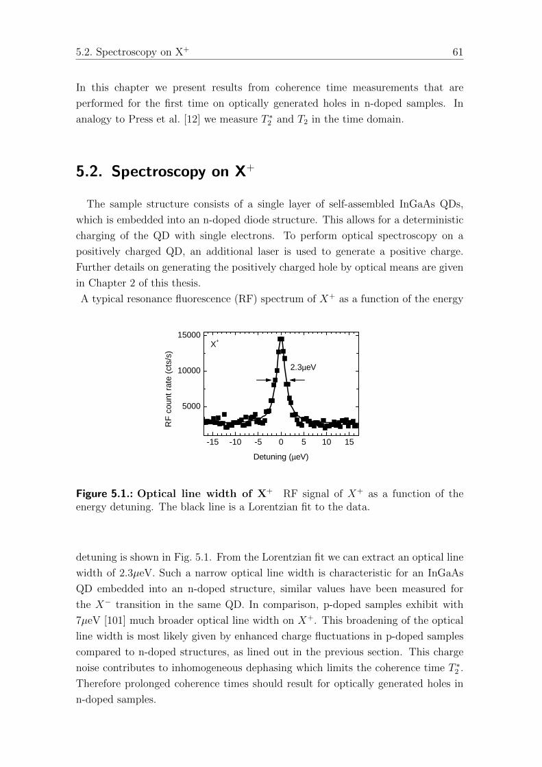
5.2. Spectroscopy on X+ 61
In this chapter we present results from coherence time measurements that are
performed for the first time on optically generated holes in n-doped samples. In
analogy to Press et al. [12] we measure T ∗2 and T2 in the time domain.
5.2. Spectroscopy on X+
The sample structure consists of a single layer of self-assembled InGaAs QDs,
which is embedded into an n-doped diode structure. This allows for a deterministic
charging of the QD with single electrons. To perform optical spectroscopy on a
positively charged QD, an additional laser is used to generate a positive charge.
Further details on generating the positively charged hole by optical means are given
in Chapter 2 of this thesis.
A typical resonance fluorescence (RF) spectrum of X+ as a function of the energy
- 1 5 - 1 0 - 5 0 5 1 0 1 5
5 0 0 0
1 0 0 0 0
1 5 0 0 0
RF co
unt ra
te (ct
s/s)
D e t u n i n g ( µe V )
2 . 3 µe V
X +
Figure 5.1.: Optical line width of X+ RF signal of X+ as a function of theenergy detuning. The black line is a Lorentzian fit to the data.
detuning is shown in Fig. 5.1. From the Lorentzian fit we can extract an optical line
width of 2.3µeV. Such a narrow optical line width is characteristic for an InGaAs
QD embedded into an n-doped structure, similar values have been measured for
the X− transition in the same QD. In comparison, p-doped samples exhibit with
7µeV [101] much broader optical line width on X+. This broadening of the optical
line width is most likely given by enhanced charge fluctuations in p-doped samples
compared to n-doped structures, as lined out in the previous section. This charge
noise contributes to inhomogeneous dephasing which limits the coherence time T ∗2 .
Therefore prolonged coherence times should result for optically generated holes in
n-doped samples.

62 Coherence of Optically Generated Hole Spins
5.3. Initialization and Readout
Reliable initialization and readout mechanisms are a prerequisite for a coherent
manipulation of a single hole spin. In the first part of this section the initialization
of the hole qubit into the spin up state is discussed. For this purpose, hole spin
pumping is used [15, 78]. The initialization mechanism is schematically shown in
Fig. 5.2 (b). First, we apply a finite transverse magnetic field (Voigt geometry).
This leads to a Zeeman splitting of the hole spin states. In Voigt geometry, the
diagonal transitions |⇓⇑↓>→|⇑> and |⇑⇓↑>→|⇑> are allowed. After exciting
the |⇓>→|⇓⇑↓> transition with a laser, the decay takes place via the diagonal
transition to |⇑> or back to the ground state |⇓> with equal probabilities. Since the
pumping rate to |⇑> is larger than the decay rate of the hole spin, an initialization
into the hole spin up state |⇑> can be achieved leading to a reduced absorption
of the laser and here in a reduced RF signal. The sample used in this work
exhibits incomplete spin pumping. This is why there is still 30% of the signal left.
Experimental evidence that the diagonal transitions are allowed is given with a
single laser RF measurement. Corresponding data is shown in Fig. 5.2 (a). Four
transitions are visible in the color coded plot of RF count rate as a function of gate
voltage and laser wavelength.
In contrast to X−, spin pumping for holes is possible without any external
-1750 -1500 -1250 -1000 -750 -500
970.62
970.60
970.58
970.56
970.54
970.52
970.50
Gate Voltage (mV)
Wavele
ngth
(nm
)
(b)
ghμBBx
WL
geμBBx
(a)
A
Figure 5.2.: X+ in Voigt geometry. (a) RF measurement of X+ versus gatevoltage and laser wavelength in an in-plane field of 4T (Voigt geometry). At thegate voltage indicated with A, Ramsey measurements are performed. The resultsare presented in section 5.7. (b) Energy level diagram for hole spin pumping. Afterresonantly exciting |⇓>→|⇓⇑↓> , the allowed diagonal transition in Voigt geometry,|⇓⇑↓>→|⇑>, leads to hole spin pumping.
magnetic field. This is due to the limited hyperfine interaction of holes with nuclear
spins resulting in a larger pump rate compared to the hole spin relaxation time [78].
Due to the fact that diagonal transitions are allowed in Voigt geometry, hole

5.4. Rabi Oscillations 63
spin pumping is even more efficient for finite magnetic fields and shows the same
magnetic field dependence as for electron spin pumping [15, 105]. An advantage of
this simple initialization process in Voigt geometry is the fact that it can be used as
well for the readout. If the laser is resonantly applied to the |⇓>→|⇓⇑↓> transition,
the RF signal strength is proportional to the occupation of the ground state |⇓>.
The coherent oscillation between the two hole spin states |⇓> and |⇑> is measured
as a projection onto the z-axis. The respective oscillation of the occupation in the
ground state |⇓> is therefore directly measured via the RF signal strength.
5.4. Rabi Oscillations
(b) (a) x basis
z basis
z
z
z
z
Wrot
wx
Wrot
ħwx
Figure 5.3.: Scheme for Rabi oscillations. (a) Level diagram in x basis forfinite magnetic field Bx. A slightly detuned (210MHz) circularly polarized rotationpulse is driving all four transitions, which are linearly polarized in Voigt geometry.(b) Level diagram in z basis for finite magnetic field Bx. Bx results into a Larmorprecession of the hole spins around the x-axis (red arrow).
After initializing the hole spin state by optical pumping, a spin rotation (Rabi
oscillation) is performed with a 4ps long, σ+ polarized laser pulse. To avoid a
population of the excited state, the laser is additionally detuned by ∆ = 210GHz.
The effect of the laser pulse can be easily understood with the help of the schematic
drawing in Fig. 5.3. In the x-basis the hole spin in the ground state is either
parallel or antiparallel to the applied magnetic field Bx. All optical transitions are
linearly polarized due to the optical selection rules in Voigt geometry. Because
we use a circularly polarized laser pulse, all four transitions are driven (Fig. 5.3
(a)). Now we consider the same situation in the z-basis (Fig. 5.3 (b)), where the
hole spin orientation is along the growth direction. In this case the two allowed
optical transitions are circularly polarized, which means that Ωrot drives only one

64 Coherence of Optically Generated Hole Spins
optical transition. Additionally, the Zeeman splitting due to Bx results in coherent
mixing of the ground and excited states. After the initialization of the hole spin in
|⇑>x= eiφ/2 |⇑>z +e−iφ/2 |⇓>z, the laser pulse induces an ac-Stark shift of |⇑>z
relative to |⇓>z. Thereby, a relative phase shift φ occurs, that is proportional to
the laser pulse duration and the laser power Prot. In other words, a laser pulse is
equivalent to an effective magnetic field along the z-axis which induces coherent
oscillations between |⇑> and |⇓>. (If not indicated with an index, |⇑> and |⇓>are in the x-basis.)
Due to the fact that every hole spin state can be represented by a superposition
of the states |⇓> and |⇑> and their relative phase, spin manipulations are best
visualized on a unit sphere called Bloch sphere. A schematic drawing of the Rabi
oscillations on the Bloch sphere is shown in Fig. 5.4 (a). After the initialization in
the |⇑> state, a rotation of the hole spin around the z-axis by an arbitrary angle
can be achieved if the rotation pulse power Prot is chosen correspondingly.
To determine the laser pulse power corresponding to a π pulse, the emitted
0.0 0.5 1.0 1.5 2.0 2.5
500
1000
1500
π
RF c
ount
rate
(cts
/0.1
s)
Prot/Pπ
a) b)
y z
x
Figure 5.4.: Rabi oscillations. (a) Visualization of Rabi oscillations on the Blochsphere. The dark red arrow indicates the initialization in the |⇑> state. With thelaser power, the rotation angle between |⇑> and |⇓> can be controlled (light redarrows). (b) Rabi oscillations between the hole spin states are observed in theoscillating RF signal as the rotation pulse power is increased.
RF photons are measured according to the readout scheme as described above.
Fig. 5.4 (b) shows the oscillating RF count rate as a function of the normalized
laser power Prot. As a consequence of the applied readout scheme, the maximal
number of photons indicates the maximal occupation of the |⇓> state. Because the
experiment is initialized in the |⇑> state, the laser power at the maximal count
rate corresponds to a π rotation on the Bloch sphere. As a result of the previously
mentioned imperfect hole spin pumping, the visibility of the Rabi oscillation is

5.5. Ramsey measurements 65
reduced. This explains that the minimal observed photon number is 250cts/0.1s
above the dark count rate of the APD. A reduced visibility, however, has no
influence on the accuracy of the determination of Pπ. The accurate control over the
rotation angle between |⇑> and |⇓> allows to conduct Ramsey experiments and
hence the determination of the coherence time T ∗2 .
5.5. Ramsey measurements
a) b) c)
y z
xBx
Figure 5.5.: Ramsey scheme. (a) After initialization in the |⇑> state, a π/2pulse is applied. (b) The in plane field leads to a rotation of the hole spin aroundthe vertical axis at the Larmor frequency. (c) The rotation is stopped after a delaytime τ with a second π/2 pulse. Depending on the phase evolution, the π/2 pulsebrings the spin back to its initial state |⇑> or to the opposite spin state |⇓>.
With the Rabi experiments in the previous section, we demonstrated that a rota-
tion of the hole spin by an arbitrary angle around the z-axis is feasible. To have a
full control over the Bloch sphere, a rotation around a second axis is needed. with
the in plane magnetic field causing a Larmor precession of the hole spin, a rotation
around the x-axis is established. This effect is exploited for Ramsey interferometry.
In a first step after initialization, a π/2 pulse is applied, that brings the hole spin
to the equator of the Bloch sphere. During the subsequent delay time τ the spin
rotates around the x-axis at the Larmor frequency. The phase evolution determines
the probability of bringing the spin back to either the initial state or to the opposite
spin state with a second π/2 pulse applied after the time τ (Fig. 5.5). Finally, the
measurement of the spin population as a function of the delay time τ leads to a
sinusoidal oscillation of the RF counts at the Larmor frequency (Ramsey fringes).
The effective magnetic field causing the Larmor precession varies slightly in time
and so does the precession frequency. Therefore, averaging that is needed to obtain
a reasonable signal strength leads to an exponential decay of the Ramsey fringes
with a time constant T ∗2 .
To experimentally achieve two π/2 pulses separated by a delay time τ , the laser
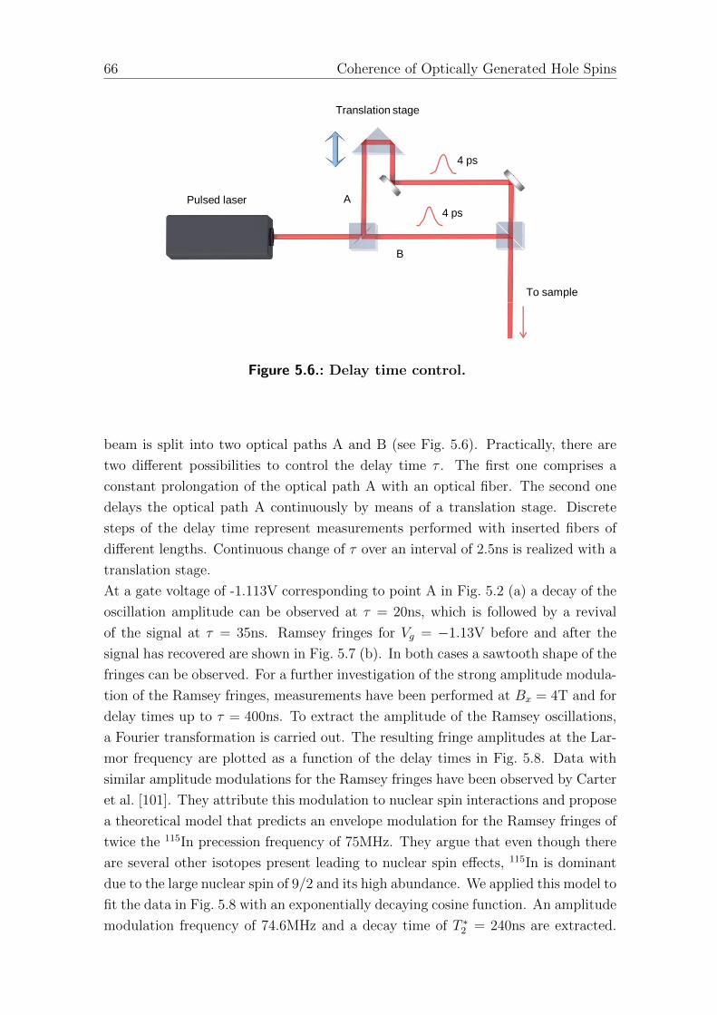
66 Coherence of Optically Generated Hole Spins
Translation stage
B
A
4 ps
4 ps
To sample
Pulsed laser
Figure 5.6.: Delay time control.
beam is split into two optical paths A and B (see Fig. 5.6). Practically, there are
two different possibilities to control the delay time τ . The first one comprises a
constant prolongation of the optical path A with an optical fiber. The second one
delays the optical path A continuously by means of a translation stage. Discrete
steps of the delay time represent measurements performed with inserted fibers of
different lengths. Continuous change of τ over an interval of 2.5ns is realized with a
translation stage.
At a gate voltage of -1.113V corresponding to point A in Fig. 5.2 (a) a decay of the
oscillation amplitude can be observed at τ = 20ns, which is followed by a revival
of the signal at τ = 35ns. Ramsey fringes for Vg = −1.13V before and after the
signal has recovered are shown in Fig. 5.7 (b). In both cases a sawtooth shape of the
fringes can be observed. For a further investigation of the strong amplitude modula-
tion of the Ramsey fringes, measurements have been performed at Bx = 4T and for
delay times up to τ = 400ns. To extract the amplitude of the Ramsey oscillations,
a Fourier transformation is carried out. The resulting fringe amplitudes at the Lar-
mor frequency are plotted as a function of the delay times in Fig. 5.8. Data with
similar amplitude modulations for the Ramsey fringes have been observed by Carter
et al. [101]. They attribute this modulation to nuclear spin interactions and propose
a theoretical model that predicts an envelope modulation for the Ramsey fringes of
twice the 115In precession frequency of 75MHz. They argue that even though there
are several other isotopes present leading to nuclear spin effects, 115In is dominant
due to the large nuclear spin of 9/2 and its high abundance. We applied this model to
fit the data in Fig. 5.8 with an exponentially decaying cosine function. An amplitude
modulation frequency of 74.6MHz and a decay time of T ∗2 = 240ns are extracted.

5.5. Ramsey measurements 67
5 10 15 20 25 30 350
1000
2000
3000
4000
5000
6000
Vg=-1130mV
RF
count
rate
(cts
/0.5
s)
Delay (ns)
34.5 35.0 35.5 36.00
1000
2000
3000
4000
5000
6000
RF
count
rate
(cts
/0.5
s)
Delay (ns)
4.0 4.5 5.0 5.50
1000
2000
3000
4000
5000
6000
RF
count
rate
(cts
/0.5
s)
Delay (ns)
(a)
(b)
p/2 p/2
t
Figure 5.7.: Ramsey fringes. (a) Ramsey fringes measured for two different tran-sitions in X+, shown in Fig. 5.2 (a) . A decay and revival of the oscillation amplitudecan be observed. (b) Magnification of the of a 1.5ns delay window highlighted witha red box in (a), to display the Ramsey fringe shape. After the revival of the oscilla-tion amplitude, at τ = 36ns, oscillations can still be observed with almost unchangedvisibility.
The modulation frequency matches within the measurement uncertainty twice the
expected 115In precession frequency of 75MHz. Not only the amplitude modulation
but also the sawtooth pattern of the Ramsey fringes can be explained with nuclear
spin polarization as follows [101]. Because a different polarization is achieved for
each delay time, the Overhauser shift changes the optical transition relative to the
laser. Therefore, the initialization and measurement process is disturbed, resulting
in the observed sawtooth pattern of the Ramsey fringes. Similar asymmetric pat-
terns were observed in Ramsey experiments with electron spins. [106, 107].

68 Coherence of Optically Generated Hole Spins
5 0 1 0 0 1 5 0 2 0 0 2 5 0 3 0 0 3 5 0 4 0 005 0
1 0 01 5 02 0 02 5 03 0 03 5 04 0 0
fringe
ampli
tude (
cts/0.
5s)
D e l a y ( n s )
T 2 * = 2 4 0 n s
Figure 5.8.: T ∗2 measurement. Ramsey fringe amplitude versus delay time witha decaying cosine fit at Bx = 4T. The extracted time constant of the exponentialdecay is T ∗2 =240ns.
5.6. Spin Echo measurements
y z
x
a) b) c)
Bx
Figure 5.9.: Spin echo scheme. (a) After initialization into the |⇑> state, a π/2pulse is applied. (b) The effective magnetic field varies for consecutive measure-ments. Some spins precess slower around the vertical axis because of the smaller fieldstrength (green arrow) and some spins precess faster due to a larger field strength(blue arrow). By applying a π pulse after a time delay T , the slower spins are nowahead of the faster precessing spins. (c) Complete refocusing takes place after atime delay T . Depending on the phase evolution, the π/2 pulse brings the spin backto its initial state or to the opposite spin state.
As it was discussed earlier, T ∗2 can be limited due to inhomogeneous dephasing
that arises from slow fluctuations in the nuclear spin polarization as well as from
charge fluctuations. To circumvent such slow sources of decoherence, spin echo
measurements are carried out.
The advantage of the spin echo measurement over Ramsey experiments is explained
by means of the schematic illustrations in Fig. 5.9. After initialization of the hole

5.6. Spin Echo measurements 69
T+t T-t
p/2 p p/2
4.6 4.8 5.0 5.2 5.4 5.6400
450
500
550
600
650400
450
500
550
600
650400
450
500
550
600
650
4.6 4.8 5.0 5.2 5.4 5.6
T=1467ns
T=204ns
Time offset t (ns)
RF
co
unt
rate
(cts
/0.5
s)
T=630ns
Figure 5.10.: Spin echo measurements. Spin-echo signal as the time offset τ isvaried, for a time delay of 2T = 1467ns, 630ns, 240ns from top to bottom. Magneticfield Bx=4 T.
spin into |⇑>, a π/2 pulse is applied. As lined out before, the effective magnetic
field and therefore the precession frequency around the x-axis are slightly different
for consecutive measurements. This leads to different precession frequencies in the
horizontal plane of the Bloch sphere, as indicated with colored arrows in Fig. 5.9
(b). To rephase the system, an additional π pulse is applied after a delay time T .
Similar to the Ramsey measurements, a second π/2 pulse is then applied and the
spin population is measured as a function of the time offset τ [60, 61]. This measure
to rephase the spins in different realizations of the experiment is effective, as long
as the fluctuations of Beff are slow compared to T .
The spin-echo signal for three different time delays T is shown as a function of
the time offset τ in Fig. 5.10. Between a time delay of T = 204ns and T = 630ns,
only very little decay in the amplitude is observed. For the longest time delay at
T = 1467ns only 10% of the signal amplitude remains. Even though there are not
enough data points for fitting an exponential decay to the signal amplitudes, the

70 Coherence of Optically Generated Hole Spins
decay time T2 can be estimated to be on the order of 1µs.
5.7. Discussion
We demonstrated experimentally that ultrafast coherent control techniques work
as well for optically generated hole spins as for electron spins in n-doped samples.
From Ramsey measurements we extracted a T ∗2 time of 240ns for optically generated
hole spins. This is a 1-2 order of magnitude larger value than what was measured
with the same method for hole spins in p-doped samples (T ∗2 = 2.3−19ns) [99, 101].
As discussed in the introduction the T ∗2 time is the longer, the less pronounced the
effects of inhomogeneous dephasing are. In other words, n-doped samples exhibit
either less charge noise or weaker fluctuations in the nuclear spin polarization. A
comparison of the optical line widths in X+ reveals for n-doped samples 2-3µeV
which is a much smaller value than the measured 7µeV for p-doped structures.
This large difference can only be caused by charge fluctuations. For that reason
smaller charge induced spectral diffusion does most likely lead to a longer T ∗2coherence time in n-doped samples compared to p-doped structures. To summarize
our results, the method of optically generating holes in QDs brings clear advantages
over conventional techniques.
By contrast, the measured spin echo time T2 for optically generated holes (T2 = 1µs)
and p-doped samples (T2 = 1.1µs) are comparable. Most interestingly also the T2
times for electrons are with 3µs in the same range. Based on dipole dipole interac-
tions of nuclear spins Witzel et al. [108] and Yao et al. [109] predict T2 ∼ 1− 10µs
for a single electron in a QD. In self-assembled QDs this nuclear spin diffusion is
negligible because of the quadrupolar interactions. Recent experiments revealed
that electron mediated nuclear spin diffusion and co - tunneling rather limit the
T2 time [79]. The measured values for T2 are rather surprising, since the weaker
interaction of hole spins with nuclear spins compared to electrons should result
in a longer T2 value. Hence, the limiting factor for the spin echo time of holes
cannot be nuclear spin effects. For p-doped samples, it is very likely that charge
induced spectral diffusion, which already limits T ∗2 , sets an upper boundary for
T2 as well. Regarding charge noise, optically generated holes in n-doped samples
are less affected which should result, compared to p-doped structures, in a longer
spin echo time. Because such a behavior is not observed, it is very probable that
the hole generating process with a weak off-resonant laser is limiting the coherence
properties. To test this hypothesis, hole spin lifetime measurements should be
carried out as a next step.
As expected from the weaker hyperfine interaction of holes with nuclear spins
compared to electrons in InGaAs QDs [19, 44, 96–98], the measured decoherence

5.7. Discussion 71
time T ∗2 = 240ns is longer than for electrons (T ∗2 = 1 − 2ns) [61]. The hole spin
decay is dependent on the orientation of the external magnetic field. This arises
from the simple Ising form∑
k AhkI
zksz that couples the hole to the nuclear spin
system, where Ahk is the coupling of the kth nucleus and Izk and sz denote the z
component of the kth nuclear spin and the hole spin, respectively. In the case of a
transverse magnetic field Bx the nuclear spin fluctuations are perpendicular to the
applied field Bx, resulting in a slow power-law hole spin decay which is estimated to
be on the order of µs. In comparison for zero field or an external field Bz the decay
is Gaussian, similar to electrons, with timescales of tens of nanoseconds [19]. Hence,
the measured two orders of magnitude longer T ∗2 for holes compared to electrons
can be explained with the weak coupling of holes to the nuclear spin system in
transverse magnetic fields.
Even though the interaction between holes and nuclear spins is weak, a strong
amplitude modulation of the Ramsey interference fringes is observed. This is a
result of nuclear spin polarization. It changes the optical transition relative to the
laser via the Overhauser shift leading to an amplitude modulation and a sawtooth
shape of the Ramsey interference fringes [101].
In addition to the results we presented above, our work gives rise to a num-
ber of further investigations. For instance, the fact that n-doped samples allow
to charge the same QD either with an electron or with a hole could be exploited
to directly compare the coherence behavior of both species. This might give new
insights into the interaction of electrons and holes with nuclear spins.
For several interesting experiments it is crucial to achieve a long coherence time. In
particular we have shown that optically generated holes in QDs are promising to
further prolong the spin echo time T2. With their work on quantum teleportation
between a photon and a single electron spin qubit, Gao et al. [107] show in which
direction research might head. Their experiments in combination with longer
coherence time could lead to a realization of spin spin entanglement.


Appendix A
A. Appendix
A.1. Experimental Setup
With a confocal microscope [110] resonant spectroscopy was performed. On the
one hand this allows for a small spot size of ∼ 1µm which is crucial for single QD
spectroscopy, on the other hand a large amount of light emitted from the QD can
be collected with a large numerical aperture (NA) of the objective. The numerical
aperture NA ∝ sinθ ∼ θ is proportional to the half angle θ of the light cone from
a lens that is illuminated with a plane wave. Therefore a higher NA increases the
collection efficiency. We performed all experiments with the lens L1 (see Fig. A.1)
that exhibits an NA of 0.68. Additionally, we used a solid immersion lens (SIL) to
increase the collection efficiency of the emitted light from the sample surface [111].
A four times increased collection efficiency was experimentally observed by compar-
ing the same sample with and without SIL.
To position the QD into the focal spot, the sample is mounted on piezoelectric
xyz-positioners. The described microscope together with the positioners and the
sample are placed inside a bath cryostat which reaches temperatures of 1.4K. Such
low temperatures are necessary to prevent temperature broadening of the QD reso-
nances. Magnetic fields up to 12T can be applied with a superconducting split coil
magnet. This geometry allows for an optical access of the sample along two different
axes. Therefore upon rotation of the sample, a magnetic field transverse (shown in
Fig. A.1) or along the growth direction can be applied.
For PL measurements the QD is excited with diode laser at 780nm, the emitted
photons from the QD are dispersed with a spectrometer (SP) of 75cm focal length
and finally analyzed with a liquid nitrogen cooled, back-illuminated CCD array.
To perform resonant spectroscopy or PLE, two tunable diode lasers (Toptica DL
pro) were available with a tuning range from 915nm to 990nm. The required in-
tensity stabilization for resonant measurement is realized with a double-pass AOM
setup [112], before the lasers are coupled into a fiber. While the dT signal is directly
measured with the photodiode PD1, the dR signal is first coupled into a single mode
fiber (CF) before it is measured on a photodiode. The additional single mode fiber
allows for a mode filtering, which is especially needed in RF measurements. In both
cases, dR/R and dT/T, after passing a preamplifier, the signal is sent to a Lock-

B Appendix
In amplifier. The Lock-In amplifier is synchronized with a function generator that
produces a square wave modulation with a DC offset which is applied to the gate of
the sample. Because of the Stark-shift, the QD transition is modulated in and out
of resonance. This technique is called Stark-shift modulation [31, 71] and allows to
suppress noise on all frequencies except the modulation frequency which is usually
at 777Hz.
Polarization control is needed to perform resonance fluorescence (RF) measurements.
By choosing the polarizer P2 cross-polarized to the polarizer P4 in front of the sin-
gle mode collection fiber (CF) an extinction ratio of ∼ 106 can be achieved. For
RF measurements it is very difficult to optimize the QD position by monitoring
the signal, because every change of the sample position leads to an increase of the
background. To align the setup and to monitor the QD position a CCD camera (C)
was used.
Hanle measurements were performed with a polarization control consisting of the
two polarizers P2 and P3 together with the liquid crystal devices (LCW, LCR). The
light polarization at the QD is determined by the fixed vertical polarizer P2 and the
liquid crystal waveplate LCW, that allows for a retardance between λ/4 and 3λ/4.
The reflected PLE laser photons from the QD experience the same retardance and
are therefore linearly polarized after the LCW. To distinguish between co- and cross
polarized QD photons a liquid crystal rotator in combination with a linear polarizer
P3 were used. To filter out the strong pump laser in PLE experiments a longpass
filter (LP) at 950nm is needed. The typical broad lasing background of a diode laser
is filtered out with a short pass (SP) at 940nm, such that it is not overwhelming the
QD emission at ∼ 960nm.
For a resonant measurement of the Overhauser shift an independent polarization
control of the pump laser La2 and the probe laser La1 is needed, therefore we placed
the LCW directly after the resonant laser (see Fig. A.1). In combination with the
fixed vertical polarizer P1, a complete polarization control of the resonant laser is
achieved. With an additional λ/4 plate, the pump laser is circularly polarized that
allows for polarizing nuclear spins in the QD. Besides the long pass filter, a grating
(G) is needed in front of the collection fiber to filter out the strong pump laser.
The creation of the laser pulses necessary for the resonant measurement of the Over-
hauser shift was performed either with an acousto-optical modulator (AOM) from
Crystal Technology, model no.3080-125 or with an electro-optical modulator (EOM)
based intensity modulator from Jenoptik AM940b. In both cases the laser pulses
were fiber coupled to separate the alignement from the measurement setup presented
in Fig. A.1.
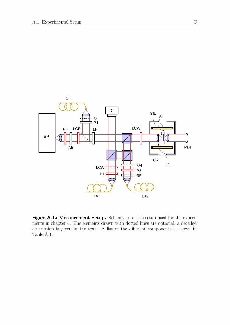
A.1. Experimental Setup CSetup for PLE measurements
SP
P2
P3
LCW
P1
LCW
CR
PD1
LCR LP
SP
C SIL
S
La1 La2
CF
l/4
P4
L1
G
Sh
Figure A.1.: Measurement Setup. Schematics of the setup used for the experi-ments in chapter 4. The elements drawn with dotted lines are optional, a detaileddescription is given in the text. A list of the different components is shown inTable A.1.

D Appendix
Item Description Manufacturer
Sp Spectrometer Princeton Instruments/Acton Research,SpectraPro 2759, f= 0.750 m
Detector Princeton Instruments, Spec-10:100BR/LN.1340×100 pixel back-illuminated CCD array
C CCD camera Watec, WAT-120NFM Flip mirror Thorlabs, BB1-E03P1,P2,P3, P4
Polarizer Thorlabs LPNIR050
LCR Liquid crystal polarizationrotator
Meadowlark, LPR-200-0915
Sh Shutter Uniblitz, LS6ZM2LCW Liquid crystal wave plate Meadowlark, LRC-200-0915L1 Achromatic lens Thorlabs, AC050-008-B-ML, NA=0.68SIL Solid immersion lens A.W.I. Industries. hemispherical ball lens,
ZrO2, uncoated.S Sample Described in detail in chapter 2PP Piezoelectric positioners Attocube, ANPx50/LT and ANPz50/LT.
Controller ANC150/3CR Bath cryostat Oxford instruments, Spectromag with 12T
split-coil magnetG Grating Ibsen Photonics, FSTG-NIR1500-903nmLa1,La2
Tunable diode laser 1 (forPLE, dR, RF)
Topitca DL pro, coarse tuning range 915-990nm, mode-hop free tuning range 20GHz,Pmax = 40 mW
Tunable diode laser 2 Toptica DL proDiode Laser (for imagingand PL)
Melles Griot, 56IC5210, λ = 780 nm, Pmax =50 mW
CF Collection fiber (for RFand dR)
Thorlabs P3-830A-FC-5
SP Short pass filter LC-3RD/940SPLP Long pass filter LC-3RD/950LP
Table A.1.: Detailed list of the most important elements used for the setup sketchedin Fig. A.1

Bibliography I
B. Bibliography
[1] Y. Aharonov and D. Bohm, Significance of Electromagnetic Potentials in the
Quantum Theory, Phys. Rev. 115, 485 (1959).
[2] T. A. Fulton and G. J. Dolan, Observation of single-electron charging effects
in small tunnel junctions, Phys. Rev. Lett. 59, 109 (1987).
[3] K. v. Klitzing, G. Dorda, and M. Pepper, New Method for High-Accuracy
Determination of the Fine-Structure Constant Based on Quantized Hall Re-
sistance, Phys. Rev. Lett. 45, 494 (1980).
[4] M. Kroner, A. O. Govorov, S. Remi, B. Biedermann, S. Seidl, A. Badolato,
P. M. Petroff, W. Zhang, B. D. Barbour, R.and Gerardot, R. J. Warburton,
et al., The nonlinear Fano effect, Nature 451, 311 (2008).
[5] C. Latta, F. Haupt, M. Hanl, A. Weichselbaum, M. Claassen, W. Wuester,
P. Fallahi, S. Faelt, L. Glazman, J. von Delft, et al., Quantum quench of Kondo
correlations in optical absorption, Nature 474, 627 (2011).
[6] N. A. J. M. Kleemans, J. van Bree, A. O. Govorov, J. G. Keizer, G. J. Hamhuis,
R. Notzel, A. Y. Silov, and P. M. Koenraad, Many-body exciton states in self-
assembled quantum dots coupled to a Fermi sea, Nature Physics 6, 534 (2010).
[7] A. C. Johnson, J. R. Petta, J. M. Taylor, A. Yacoby, M. D. Lukin, C. M.
Marcus, M. P. Hanson, and A. C. Gossard, Triplet-singlet spin relaxation via
nuclei in a double quantum dot, Nature 435, 925 (2005).
[8] P. Maletinsky, A. Badolato, and A. Imamoglu, Dynamics of Quantum Dot
Nuclear Spin Polarization Controlled by a Single Electron, Phys. Rev. Lett.
99, 056804 (2007).
[9] M. Kroutvar, Y. Ducommun, D. Heiss, M. Bichler, D. Schuh, G. Abstreiter,
and J. J. Finley, Optically programmable electron spin memory using semicon-
ductor quantum dots, Nature 432, 81 (2004).
[10] H. Bluhm, S. Foletti, I. Neder, M. Rudner, D. Mahalu, and A. Yacoby, De-
phasing time of GaAs electron-spin qubits coupled to a nuclear bath exceeding
200µs, Nature Physics 7, 109 (2011).

II Bibliography
[11] D. Brunner, B. D. Gerardot, P. A. Dalgarno, G. Wust, K. Karrai, N. G.
Stoltz, P. M. Petroff, and R. J. Warburton, A Coherent Single-Hole Spin in a
Semiconductor, Science 325, 70 (2009).
[12] D. Press, T. D. Ladd, B. Zhang, and Y. Yamamoto, Complete quantum control
of a single quantum dot spin using ultrafast optical pulses, Nature 456, 218
(2008).
[13] J. Berezovsky, M. H. Mikkelsen, N. G. Stoltz, L. A. Coldren, and D. D.
Awschalom, Picosecond Coherent Optical Manipulation of a Single Electron
Spin in a Quantum Dot, Science 320, 349 (2008).
[14] D. Loss and D. P. DiVincenzo, Quantum computation with quantum dots,
Phys. Rev. A 57, 120 (1998).
[15] M. Atature, J. Dreiser, A. Badolato, A. Hogele, K. Karrai, and A. Imamoglu,
Quantum-Dot Spin-State Preparation with Near-Unity Fidelity, Science 312,
551 (2006).
[16] F. H. L. Koppens, C. Buizert, K. J. Tielrooij, I. T. Vink, K. C. Nowack,
T. Meunier, L. P. Kouwenhoven, and L. M. K. Vandersypen, Driven coherent
oscillations of a single electron spin in a quantum dot, Nature 442, 766 (2006).
[17] I. A. Merkulov, A. L. Efros, and M. Rosen, Electron spin relaxation by nuclei
in semiconductor quantum dots, Phys. Rev. B 65, 205309 (2002).
[18] H. Bluhm, S. Foletti, D. Mahalu, V. Umansky, and A. Yacoby, Enhancing the
Coherence of a Spin Qubit by Operating it as a Feedback Loop That Controls
its Nuclear Spin Bath, Phys. Rev. Lett. 105, 216803 (2010).
[19] J. Fischer, W. A. Coish, D. V. Bulaev, and D. Loss, Spin decoherence of a
heavy hole coupled to nuclear spins in a quantum dot, Phys. Rev. B 78, 155329
(2008).
[20] O. Krebs, P. Maletinsky, T. Amand, B. Urbaszek, A. Lemaitre, P. Voisin,
X. Marie, and A. Imamoglu, Anomalous Hanle Effect due to Optically Created
Transverse Overhauser Field in Single InAs/GaAs Quantum Dots, Phys. Rev.
Lett. 104, 056603 (2010).
[21] R. Hanson, L. P. Kouwenhoven, J. R. Petta, S. Tarucha, and L. M. K. Vander-
sypen, Spins in few-electron quantum dots, Rev. Mod. Phys. 79, 1217 (2007).
[22] A. Alivisatos, Semiconductor lusters, nanocrystals, and quantum dots, Science
271, 933 (1996).

III
[23] I. L. Medintz, H. T. Uyeda, E. R. Goldman, and H. Mattoussi, Quantum
dot bioconjugates for imaging, labelling and sensing, Nature Materials 4, 435
(2005).
[24] L. Biadala, Y. Louyer, P. Tamarat, and B. Lounis, Band-Edge Exciton Fine
Structure of Single CdSe/ZnS Nanocrystals in External Magnetic Fields, Phys.
Rev. Lett. 105, 157402 (2010).
[25] D. Leonard, M. Krishnamurthy, C. M. Reaves, S. P. Denbaars, and P. M.
Petroff, Direct formation of quantum-sized dots from uniform coherent islands
of InGaAs on GaAs surfaces, Applied Physics Letters 63 (1993).
[26] A. V. Kuhlmann, J. Houel, A. Ludwig, L. Greuter, D. Reuter, A. D. Wieck,
M. Poggio, and R. J. Warburton, Charge noise and spin noise in a semicon-
ductor quantum device, Nature Physics 9, 570 (2013).
[27] P. Michler, A. Kiraz, C. Becher, W. V. Schoenfeld, P. M. Petroff, L. Zhang,
E. Hu, and A. Imamoglu, A Quantum Dot Single-Photon Turnstile Device,
Science 290, 2282 (2000).
[28] I. N. Stranski and L. Krastanow, Abhandlungen der Mathematisch-
Naturwissenschaftlichen Klasse, Akademie der Wissenschaften Wien 146, 797
(1938).
[29] J. M. Garcia, T. Mankad, P. O. Holtz, P. J. Wellman, and P. M. Petroff,
Electronic states tuning of InAs self-assembled quantum dots, Applied Physics
Letters 72 (1998).
[30] J. Y. Marzin, J. M. Gerard, A. Izrael, D. Barrier, and G. Bastard, Photolu-
minescence of Single InAs Quantum Dots Obtained by Self-Organized Growth
on GaAs, Phys. Rev. Lett. 73, 716 (1994).
[31] A. Hogele, S. Seidl, M. Kroner, K. Karrai, R. J. Warburton, B. D. Gerardot,
and P. M. Petroff, Voltage-Controlled Optics of a Quantum Dot, Phys. Rev.
Lett. 93, 217401 (2004).
[32] D. V. Bulaev and D. Loss, Electric Dipole Spin Resonance for Heavy Holes in
Quantum Dots, Phys. Rev. Lett. 98, 097202 (2007).
[33] M. Kroner, Ph.D. thesis, LMU Munich (2008).
[34] H. Drexler, D. Leonard, W. Hansen, J. P. Kotthaus, and P. M. Petroff, Spec-
troscopy of Quantum Levels in Charge-Tunable InGaAs Quantum Dots, Phys.
Rev. Lett. 73, 2252 (1994).

IV Bibliography
[35] R. J. Warburton, C. Schaflein, D. Haft, F. Bickel, A. Lorke, K. Karrai, J. M.
Garcia, W. Schoenfeld, and P. M. Petroff, Optical emission from a charge-
tunable quantum ring, Nature 405, 926 (2000).
[36] S. Seidl, M. Kroner, P. A. Dalgarno, A. Hogele, J. M. Smith, M. Ediger,
B. D. Gerardot, J. M. Garcia, P. M. Petroff, K. Karrai, et al., Absorption
and photoluminescence spectroscopy on a single self-assembled charge-tunable
quantum dot, Phys. Rev. B 72, 195339 (2005).
[37] M. Ediger, P. A. Dalgarno, J. M. Smith, B. D. Gerardot, R. J. Warburton,
K. Karrai, and P. M. Petroff, Controlled generation of neutral, negatively-
charged and positively-charged excitons in the same single quantum dot, Ap-
plied Physics Letters 86, 211909 (2005).
[38] M. Ediger, G. Bester, A. Badolato, P. M. Petroff, K. Karrai, A. Zunger, and
R. J. Warburton, Peculiar many-body effects revealed in the spectroscopy of
highly charged quantum dots, Nature Physics 3, 774 (2007).
[39] R. J. Warburton, C. Schulhauser, D. Haft, C. Schaflein, K. Karrai, J. M.
Garcia, W. Schoenfeld, and P. M. Petroff, Giant permanent dipole moments
of excitons in semiconductor nanostructures, Phys. Rev. B 65, 113303 (2002).
[40] C. Latta, A. Hogele, Y. Zhao, A. N. Vamivakas, P. Maletinsky, M. Kroner,
J. Dreiser, I. Carusotto, A. Badolato, D. Schuh, et al., Confluence of reso-
nant laser excitation and bidirectional quantum-dot nuclear-spin polarization,
Nature Physics 5, 758 (2009).
[41] X. Xu, W. Yao, B. Sun, D. G. Steel, A. S. Bracker, D. Gammon, and L. J.
Sham, Optically controlled locking of the nuclear field via coherent dark-state
spectroscopy, Nature 459, 1105 (2009).
[42] P. Maletinsky, C. W. Lai, A. Badolato, and A. Imamoglu, Nonlinear dynamics
of quantum dot nuclear spins, Phys. Rev. B 75, 035409 (2007).
[43] A. I. Tartakovskii, T. Wright, A. Russell, V. I. Fal’ko, A. B. Van’kov, J. Skiba-
Szymanska, I. Drouzas, R. S. Kolodka, M. S. Skolnick, P. W. Fry, et al.,
Nuclear Spin Switch in Semiconductor Quantum Dots, Phys. Rev. Lett. 98,
026806 (2007).
[44] P. Fallahi, S. T. Yilmaz, and A. Imamoglu, Measurement of a Heavy-Hole Hy-
perfine Interaction in InGaAs Quantum Dots Using Resonance Fluorescence,
Phys. Rev. Lett. 105, 257402 (2010).

V
[45] M. Bayer, A. Kuther, F. Schafer, J. P. Reithmaier, and A. Forchel, Strong
variation of the exciton g factors in self-assembled In0.60Ga0.40As quantum
dots, Phys. Rev. B 60, R8481 (1999).
[46] E. A. Chekhovich, K. V. Kavokin, J. Puebla, A. B. Krysa, M. Hopkinson, A. D.
Andreev, A. M. Sanchez, R. Beanland, M. S. Skolnick, and A. I. Tartakovskii,
Structural analysis of strained quantum dots using nuclear magnetic resonance,
Nature Nanotechnology 7, 646 (2012).
[47] A. Abragam, The principles of nuclear magnetism, International Series of
Monographs on Physics (Book 32) (Oxford University Press, USA, 1983),
ISBN 978-0198520146.
[48] M. I. Dyakonov, Spin Physics in Semiconductors (Springer Verlag Berlin Hei-
delberg, 2008).
[49] J. D. Jackson, Classical electrodynamics (Wiley, New York, NY, 1999), 3rd
ed., ISBN 9780471309321.
[50] C. Slichter, Principles of Magnetic Resonance, Lecture Notes in Computer
Science (World Publishing Company, 1990), ISBN 9783540501572.
[51] R. I. Dzhioev and V. L. Korenev, Stabilization of the Electron-Nuclear Spin
Orientation in Quantum Dots by the Nuclear Quadrupole Interaction, Phys.
Rev. Lett. 99, 037401 (2007).
[52] P. Maletinsky, K. Kroner, and A. Imamoglu, Breakdown of the nuclear-spin-
temperature approach in quantum-dot demagnetization experiments, Nature
Physics 5, 407 (2009).
[53] O. Krebs, B. Eble, A. Lematre, P. Voisin, B. Urbaszek, T. Amand,
and X. Marie, Hyperfine interaction in InAs/GaAs self-assembled quantum
dots: dynamical nuclear polarization versus spin relaxation, Comptes Rendus
Physique 9, 874 (2008), ISSN 1631-0705.
[54] A. V. Khaetskii, D. Loss, and L. Glazman, Electron Spin Decoherence in Quan-
tum Dots due to Interaction with Nuclei, Phys. Rev. Lett. 88, 186802 (2002).
[55] P.-F. Braun, B. Urbaszek, T. Amand, X. Marie, O. Krebs, B. Eble,
A. Lemaitre, and P. Voisin, Bistability of the nuclear polarization created
through optical pumping in In1−xGaxAs quantum dots, Phys. Rev. B 74,
245306 (2006).
[56] F. Meier, Optical orientation (North-Holland, Amsterdam, 1984).
VI Bibliography
[57] D. Paget, G. Lampel, B. Sapoval, and V. I. Safarov, Low field electron-nuclear
spin coupling in gallium arsenide under optical pumping conditions, Phys. Rev.
B 15, 5780 (1977).
[58] M. Issler, E. M. Kessler, G. Giedke, S. Yelin, I. Cirac, M. D. Lukin, and
A. Imamoglu, Nuclear Spin Cooling Using Overhauser-Field Selective Coher-
ent Population Trapping, Phys. Rev. Lett. 105, 267202 (2010).
[59] B. Urbaszek, X. Marie, T. Amand, O. Krebs, P. Voisin, P. Maletinsky,
A. Hogele, and A. Imamoglu, Nuclear spin physics in quantum dots: An optical
investigation, Rev. Mod. Phys. 85, 79 (2013).
[60] E. L. Hahn, Spin Echoes, Phys. Rev. 80, 580 (1950).
[61] D. Press, K. De Greve, P. L. McMahon, T. D. Ladd, B. Friess, C. Schneider,
M. Kamp, S. Hofling, A. Forchel, and Y. Yamamoto, Ultrafast optical spin
echo in a single quantum dot, Nature Photonics 4, 367 (2010).
[62] J. J. Finley, A. D. Ashmore, A. Lemaitre, D. J. Mowbray, M. S. Skolnick,
I. E. Itskevich, P. A. Maksym, M. Hopkinson, and T. F. Krauss, Charged and
neutral exciton complexes in individual self-assembled InGaAs quantum dots,
Phys. Rev. B 63, 073307 (2001).
[63] S. Trumm, M. Wesseli, H. J. Krenner, D. Schuh, M. Bichler, J. J. Finley, and
M. Betz, Spin-preserving ultrafast carrier capture and relaxation in InGaAs
quantum dots, Applied Physics Letters 87, 153113 (2005).
[64] R. Heitz, A. Kalburge, Q. Xie, M. Grundmann, P. Chen, A. Hoffmann,
A. Madhukar, and D. Bimberg, Excited states and energy relaxation in stacked
InAs/GaAs quantum dots, Phys. Rev. B 57, 9050 (1998).
[65] J. Houel, A. V. Kuhlmann, L. Greuter, F. Xue, M. Poggio, B. D. Gerardot,
P. A. Dalgarno, A. Badolato, P. M. Petroff, A. Ludwig, et al., Probing Single-
Charge Fluctuations at a GaAs/AlAs Interface Using Laser Spectroscopy on a
Nearby InGaAs Quantum Dot, Phys. Rev. Lett. 108, 107401 (2012).
[66] C. W. Lai, P. Maletinsky, A. Badolato, and A. Imamoglu, Knight-Field-
Enabled Nuclear Spin Polarization in Single Quantum Dots, Phys. Rev. Lett.
96, 167403 (2006).
[67] T. D. Visser and E. Wolf, The origin of the Gouy phase anomaly and its gener-
alization to astigmatic wavefields, Optics Communications 283, 3371 (2010).
[68] T. Gouy, Sur une propriete nouvelle des ondes lumineuses, CR Hebdomadaires
Seances Acad. Sci. 110, 1251 (1890).

VII
[69] K. Karrai and R. J. Warburton, Optical transmission and reflection spec-
troscopy of single quantum dots, Superlattices and Microstructures 33, 311
(2003), ISSN 0749-6036, special issue dedicated to Professor Jorg Kotthaus on
the occasion of his 60th Birthday, 29th May 2004.
[70] M. Kroner, S. Remi, A. Hogele, S. Seidl, A. Holleitner, R. Warburton, B. Ger-
ardot, P. Petroff, and K. Karrai, Resonant saturation laser spectroscopy of a
single self-assembled quantum dot, Physica E: Low-dimensional Systems and
Nanostructures 40, 1994 (2008), ISSN 1386-9477, 13th International Confer-
ence on Modulated Semiconductor Structures.
[71] B. Alen, F. Bickel, K. Karrai, R. J. Warburton, and P. M. Petroff, Stark-shift
modulation absorption spectroscopy of single quantum dots, Applied Physics
Letters 83 (2003).
[72] E. B. Flagg, A. Muller, J. W. Robertson, S. Founta, D. G. Deppe, M. Xiao,
W. Ma, G. J. Salamo, and C. K. Shih, Resonantly driven coherent oscillations
in a solid-state quantum emitter, Nature Physics 5, 203 (2009).
[73] A. Nick Vamivakas, Y. Zhao, C.-Y. Lu, and M. Atature, Spin-resolved
quantum-dot resonance fluorescence, Nature Physics 5, 198 (2009).
[74] S. T. Yilmaz, P. Fallahi, and A. Imamoglu, Quantum-Dot-Spin Single-Photon
Interface, Phys. Rev. Lett. 105, 033601 (2010).
[75] A. V. Kuhlmann, J. Houel, D. Brunner, A. Ludwig, D. Reuter, A. D. Wieck,
and R. J. Warburton, A dark-field microscope for background-free detection of
resonance fluorescence from single semiconductor quantum dots operating in
a set-and-forget mode, Review of Scientific Instruments 84, 073905 (2013).
[76] C. Kloeffel, P. A. Dalgarno, B. Urbaszek, B. D. Gerardot, D. Brunner, P. M.
Petroff, D. Loss, and R. J. Warburton, Controlling the Interaction of Electron
and Nuclear Spins in a Tunnel-Coupled Quantum Dot, Phys. Rev. Lett. 106,
046802 (2011).
[77] E. A. Chekhovich, M. N. Makhonin, K. V. Kavokin, A. B. Krysa, M. S. Skol-
nick, and A. I. Tartakovskii, Pumping of Nuclear Spins by Optical Excitation of
Spin-Forbidden Transitions in a Quantum Dot, Phys. Rev. Lett. 104, 066804
(2010).
[78] B. D. Gerardot, D. Brunner, P. A. Dalgarno, P. Ohberg, S. Seidl, M. Kroner,
K. Karrai, N. G. Stoltz, P. M. Petroff, and R. J. Warburton, Optical pumping
of a single hole spin in a quantum dot, Nature 451, 441 (2008).

VIII Bibliography
[79] C. Latta, A. Srivastava, and A. Imamoglu, Hyperfine Interaction-Dominated
Dynamics of Nuclear Spins in Self-Assembled InGaAs Quantum Dots, Phys.
Rev. Lett. 107, 167401 (2011).
[80] H. J. Carmichael, Analystical and numerical results for the steady state in
cooperative reasonance fluorescence, J. Phys. B 13, 3551 (1980).
[81] P. Werner, K. Volker, M. Troyer, and S. Chakravarty, Phase Diagram and
Critical Exponents of a Dissipative Ising Spin Chain in a Transverse Magnetic
Field, Phys. Rev. Lett. 94, 047201 (2005).
[82] S. Diehl, A. Tomadin, A. Micheli, R. Fazio, and P. Zoller, Dynamical Phase
Transitions and Instabilities in Open Atomic Many-Body Systems, Phys. Rev.
Lett. 105, 015702 (2010).
[83] E. M. Kessler, G. Giedke, A. Imamoglu, S. F. Yelin, M. D. Lukin, and J. I.
Cirac, Dissipative phase transition in a central spin system, Phys. Rev. A 86,
012116 (2012).
[84] G. Sallen, S. Kunz, T. Amand, L. Bouet, T. Kuroda, T. Mano, D. Paget,
O. Krebs, X. Marie, K. Sakoda, et al., Nuclear magnetization in gallium ar-
senide quantum dots at zero magnetic field, arXiv:1309.1288 (2013).
[85] D. V. Regelman, E. Dekel, D. Gershoni, E. Ehrenfreund, A. J. Williamson,
J. Shumway, A. Zunger, W. V. Schoenfeld, and P. M. Petroff, Optical spec-
troscopy of single quantum dots at tunable positive, neutral, and negative
charge states, Phys. Rev. B 64, 165301 (2001).
[86] M. Bayer, G. Ortner, O. Stern, A. Kuther, A. A. Gorbunov, A. Forchel,
P. Hawrylak, S. Fafard, K. Hinzer, T. L. Reinecke, et al., Fine structure of
neutral and charged excitons in self-assembled In(Ga)As/(Al)GaAs quantum
dots, Phys. Rev. B 65, 195315 (2002).
[87] X. Xu, Y. Wu, B. Sun, Q. Huang, J. Cheng, D. G. Steel, A. S. Bracker,
D. Gammon, C. Emary, and L. J. Sham, Fast Spin State Initialization in a
Singly Charged InAs-GaAs Quantum Dot by Optical Cooling, Phys. Rev. Lett.
99, 097401 (2007).
[88] S. Haroche and J.-M. Raimond, Exploring the Quantum - Atoms, Cavities and
Photons (Oxford University press Inc. New York, 2006).
[89] A. Hogele, M. Kroner, C. Latta, M. Claassen, I. Carusotto, C. Bulutay, and
A. Imamoglu, Dynamic Nuclear Spin Polarization in the Resonant Laser Ex-
citation of an InGaAs Quantum Dot, Phys. Rev. Lett. 108, 197403 (2012).

IX
[90] C. Bulutay, Quadrupolar spectra of nuclear spins in strained InGaAs quantum
dots, Phys. Rev. B 85, 115313 (2012).
[91] P. Maletinsky, Ph.D. thesis, ETH Zurich (2008).
[92] A. Imamoglu, D. D. Awschalom, G. Burkard, D. P. DiVincenzo, D. Loss,
M. Sherwin, and A. Small, Quantum Information Processing Using Quantum
Dot Spins and Cavity QED, Phys. Rev. Lett. 83, 4204 (1999).
[93] J. R. Petta, A. C. Johnson, J. M. Taylor, E. A. Laird, A. Yacoby, M. D. Lukin,
C. M. Marcus, M. P. Hanson, and A. C. Gossard, Coherent Manipulation of
Coupled Electron Spins in Semiconductor Quantum Dots, Science 309, 2180
(2005).
[94] A. Greilich, S. E. Economou, S. Spatzek, D. R. Yakovlev, D. Reuter, A. D.
Wieck, T. L. Reinecke, and M. Bayer, Ultrafast optical rotations of electron
spins in quantum dots, Nature Physics 5, 262 (2009).
[95] E. D. Kim, K. Truex, X. Xu, B. Sun, D. G. Steel, A. S. Bracker, D. Gammon,
and L. J. Sham, Fast Spin Rotations by Optically Controlled Geometric Phases
in a Charge-Tunable InAs Quantum Dot, Phys. Rev. Lett. 104, 167401 (2010).
[96] B. Eble, C. Testelin, P. Desfonds, F. Bernardot, A. Balocchi, T. Amand, A. Mi-
ard, A. Lemaitre, X. Marie, and M. Chamarro, HoleNuclear Spin Interaction
in Quantum Dots, Phys. Rev. Lett. 102, 146601 (2009).
[97] E. A. Chekhovich, A. B. Krysa, M. S. Skolnick, and A. I. Tartakovskii, Di-
rect Measurement of the Hole-Nuclear Spin Interaction in Single InP/GaInP
Quantum Dots Using Photoluminescence Spectroscopy, Phys. Rev. Lett. 106,
027402 (2011).
[98] E. A. Chekhovich, M. M. Glazov, A. B. Krysa, M. Hopkinson, P. Senellart,
A. Lemaitre, M. S. Skolnick, and A. I. Tartakovskii, Element-sensitive mea-
surement of the hole-nuclear spin interaction in quantum dots, Nature Physics
9, 74 (2013).
[99] K. De Greve, P. L. McMahon, D. Press, T. D. Ladd, D. Bisping, C. Schneider,
M. Kamp, L. Worschech, S. Hofling, A. Forchel, et al., Ultrafast coherent
control and suppressed nuclear feedback of a single quantum dot hole qubit,
Nature Physics 7, 872 (2011).
[100] A. Greilich, S. G. Carter, D. Kim, A. S. Bracker, and D. Gammon, Optical con-
trol of one and two hole spins in interacting quantum dots, Nature Photonics
5, 702 (2011).

X Bibliography
[101] S. G. Carter, S. E. Economou, A. Greilich, E. Barnes, A. S. Sweeney, Timothy
M. Bracker, and D. Gammon, Strong Hyperfine-Induced Modulation of an
Optically-Driven Hole Spin in an InAs Quantum Dot, arXiv:1307.3260 (2013).
[102] M. Fleischhauer, A. Imamoglu, and J. P. Marangos, Electromagnetically in-
duced transparency: Optics in coherent media, Rev. Mod. Phys. 77, 633 (2005).
[103] K.-J. Boller, A. Imamolu, and S. E. Harris, Observation of electromagnetically
induced transparency, Phys. Rev. Lett. 66, 2593 (1991).
[104] K. M. Weiss, J. M. Elzerman, Y. L. Delley, J. Miguel-Sanchez, and
A. Imamoglu, Coherent Two-Electron Spin Qubits in an Optically Active Pair
of Coupled InGaAs Quantum Dots, Phys. Rev. Lett. 109, 107401 (2012).
[105] J. Dreiser, M. Atature, C. Galland, T. Muller, A. Badolato, and A. Imamoglu,
Optical investigations of quantum dot spin dynamics as a function of external
electric and magnetic fields, Phys. Rev. B 77, 075317 (2008).
[106] T. D. Ladd, D. Press, K. De Greve, P. L. McMahon, B. Friess, C. Schneider,
M. Kamp, S. Hofling, A. Forchel, and Y. Yamamoto, Pulsed Nuclear Pumping
and Spin Diffusion in a Single Charged Quantum Dot, Phys. Rev. Lett. 105,
107401 (2010).
[107] W. Gao, P. Fallahi, E. Togan, A. Delteil, Y. Chin, J. Miguel-Sanchez, and
A. Imamoglu, Quantum teleportation from a propagating photon to a solid-
state spin qubit, Nature Communications 4, 2744 (2013).
[108] W. M. Witzel and S. Das Sarma, Quantum theory for electron spin decoherence
induced by nuclear spin dynamics in semiconductor quantum computer archi-
tectures: Spectral diffusion of localized electron spins in the nuclear solid-state
environment, Phys. Rev. B 74, 035322 (2006).
[109] W. Yao, R.-B. Liu, and L. J. Sham, Theory of electron spin decoherence by
interacting nuclear spins in a quantum dot, Phys. Rev. B 74, 195301 (2006).
[110] M. Minsky, Memoir on inventing the confocal scanning microscope, Scanning
10, 128 (1988), ISSN 1932-8745.
[111] V. Zwiller and G. Bjork, Improved light extraction from emitters in high refrac-
tive index materials using solid immersion lenses, Journal of Applied Physics
92 (2002).
[112] E. A. Donley, T. P. Heavner, F. Levi, M. O. Tataw, and S. R. Jefferts, Double-
pass acousto-optic modulator system, Review of Scientific Instruments 76,
063112 (2005).

Acknowledgements XI
Acknowledgements
First of all, I would like to thank Atac for giving me the opportunity to do my PhD
in his group. He let me accomplish many interesting and challenging experiments,
broadened my horizon with several theoretical simulations and let me explore the
world of quantum optics with a lot of freedom.
I am very thankful also to Prof. K. Ensslin for investing his valuable time in co-
examining this work.
Without knowing anything about spectroscopy techniques at the beginning of my
PhD, it would have been difficult to start my project without a good teacher in the
lab. Many thanks go to Martin who taught me how to perform proper experiments
in an optics lab. In addition I would like to thank him for many inspiring discussion
and the critical proof-reading of this manuscript.
A special thank goes to Weibo who shared his knowledge about coherent rotation of
single spins with me. Without his help the coherence time measurements on single
hole spins would not have been possible.
I would like to thank Mena for all the discussions we had, her support on simulating
nuclear spins, the proof-reading of this thesis and for being a good friend. My office
mates Charles and Francesco I would like to thank for always being open for a
little chat about physics and other subjects. Many thanks to the whole group for
their support and the after-work activities like trips to the mountains, BBQs, movie
nights and of course the delicious Christmas dinners. Especially Kathi I would like
to thank not only for the perfect administration but also for actively improving the
social life in our group.
Moreover I thank Sarah, Tina, Lars, Andreas, Andres, Susanne, Kathi, Theo and
others for their friendship. The many WOKA lunches, fondue events, hiking trips
and much more were always a good distraction from my work at ETH.
A special thank goes to Kurt who gave me an introduction to welding and helped
me realizing an additional construction for the optical table.
Finally, I would like to thank my parents Rita and Hans for the endless support and
their understanding for my more and more infrequent visits. My brother Matthias
I thank for his clean room expertise and for always believing in me. I especially
would like to thank Philip for his love, encouragement and for always supporting
my plans.


Curriculum Vitae XIII
Curriculum Vitae
Personal DetailsName Priska Barbara Studer
Date of Birth 28th of October, 1984
Place of Birth Wolhusen, Switzerland
e-mail [email protected]
Education2009 – 2014 Ph.D. in Quantum Optics
Quantum Photonics group, ETH Zurich, SwitzerlandAdvisor: Prof. Dr. Atac Imamoglu
2006– 2009 Highschool teaching diploma in PhysicsETH Zurich, Switzerland
Mar – Jun 2008 Research intern at Yale University, CT, USA
2003 – 2008 Diploma in PhysicsETH Zurich, Switzerland
1997 – 2003 Kantonsschule Willisau, Maturaoption “Physics and Applied Mathematics”
QualificationsLanguages German, English, French
Software Mathematica, LabView, Matlab, Ansoft HFSS, Origin
Additional Experience2009 – 2014 Teaching assistant in Physics, ETH Zurich, tutoring undergraduate stu-
dents
2012 – 2013 Member of the organization comittee IONS-13 SwitzerlandInternational optics conference for PhD and Master students with 100 par-ticipants from 32 countries. Responsible for student contacts, organizationand planning of travel grants
2005 – 2007 Teaching assistant at the Institute of Applied Mathematics, ETH Zurich,tutoring undergraduate students
March, 2014


List of Figures XV
List of Figures
2.1. Growth of self-assembled QDs. . . . . . . . . . . . . . . . . . . . . . . 7
2.2. Confinement in an InGaAs QD. . . . . . . . . . . . . . . . . . . . . . 8
2.3. Field effect structure. . . . . . . . . . . . . . . . . . . . . . . . . . . . 10
2.4. Charging n-doped samples with a single hole. . . . . . . . . . . . . . 11
2.5. Charging diagram measured in PL. . . . . . . . . . . . . . . . . . . . 12
3.1. dT/T measurement for X−. . . . . . . . . . . . . . . . . . . . . . . . 23
3.2. Opitcal detection of nuclear spin polarization in X+ . . . . . . . . . . 25
3.3. Comparison between dR and ∆ EOS. . . . . . . . . . . . . . . . . . . 27
3.4. Nuclear spin dynamics measured with p-shell emission. . . . . . . . . 28
3.5. Measurement scheme for pump probe with dR. . . . . . . . . . . . . . 30
3.6. dR measurement with software based Lock-In amplifier. . . . . . . . . 31
3.7. Pump probe measurement with dR. . . . . . . . . . . . . . . . . . . . 32
3.8. Pump probe measurement with dR for different Twait. . . . . . . . . . 33
3.9. Pump probe measurements with RF. . . . . . . . . . . . . . . . . . . 35
4.1. Scheme illustrating Hanle measurements. . . . . . . . . . . . . . . . . 39
4.2. Anomalous Hanle effect. . . . . . . . . . . . . . . . . . . . . . . . . . 41
4.3. Hanle measurements for different nuclear spin polarizations. . . . . . 42
4.4. Emission at the s-shell. . . . . . . . . . . . . . . . . . . . . . . . . . . 43
4.5. Hanle measurements for different sample structures . . . . . . . . . . 44
4.6. RF measurements sample A. . . . . . . . . . . . . . . . . . . . . . . . 46
4.7. Gate modulation at different frequencies. . . . . . . . . . . . . . . . . 47
4.8. CW RF measurement sample B. . . . . . . . . . . . . . . . . . . . . . 49
4.9. Extracted positions of the resonances. . . . . . . . . . . . . . . . . . . 50
4.10. Transition between Overhauser shift and Zeeman splitting. . . . . . . 51
4.11. Transition between Overhauser shift and Zeeman splitting. . . . . . . 52
4.12. Polarization dependence at Bx=0.45T. . . . . . . . . . . . . . . . . . 53
4.13. Nuclear field changes in Bx. . . . . . . . . . . . . . . . . . . . . . . . 56
5.1. Optical line width of X+. . . . . . . . . . . . . . . . . . . . . . . . . 61
5.2. X+ in Voigt geometry. . . . . . . . . . . . . . . . . . . . . . . . . . . 62
5.3. Scheme for Rabi oscillations. . . . . . . . . . . . . . . . . . . . . . . . 63
XVI List of Figures
5.4. Rabi oscillations. . . . . . . . . . . . . . . . . . . . . . . . . . . . . . 64
5.5. Ramsey scheme. . . . . . . . . . . . . . . . . . . . . . . . . . . . . . . 65
5.6. Delay time control. . . . . . . . . . . . . . . . . . . . . . . . . . . . . 66
5.7. Ramsey fringes. . . . . . . . . . . . . . . . . . . . . . . . . . . . . . . 67
5.8. T ∗2 measurement. . . . . . . . . . . . . . . . . . . . . . . . . . . . . . 68
5.9. Ramsey scheme. . . . . . . . . . . . . . . . . . . . . . . . . . . . . . . 68
5.10. Spin echo measurements. . . . . . . . . . . . . . . . . . . . . . . . . . 69
A.1. Measurement Setup. . . . . . . . . . . . . . . . . . . . . . . . . . . . C


