Reverse engineering gene and protein regulatory networks using Graphical Models.
89
Reverse engineering gene and protein regulatory networks using Graphical Models. A comparative evaluation study. Marco Grzegorczyk Dirk Husmeier Adriano Werhli
description
Reverse engineering gene and protein regulatory networks using Graphical Models. A comparative evaluation study. Marco Grzegorczyk Dirk Husmeier Adriano Werhli. Systems biology Learning signalling pathways and regulatory networks from postgenomic data. possibly completely unknown. - PowerPoint PPT Presentation
Transcript of Reverse engineering gene and protein regulatory networks using Graphical Models.

Reverse engineering gene and protein regulatory networks
using Graphical Models. A comparative evaluation study.
Marco Grzegorczyk
Dirk Husmeier
Adriano Werhli


Systems biology
Learning signalling pathways and regulatory networks from
postgenomic data


possibly completely unknown

possibly completely unknown
E.g.: Flow cytometry
experiments
data
Here: Concentrations of (phosphorylated) proteins

possibly completely unknown
E.g.: Flow cytometry
experiments
data data
Machine Learning
statistical methods
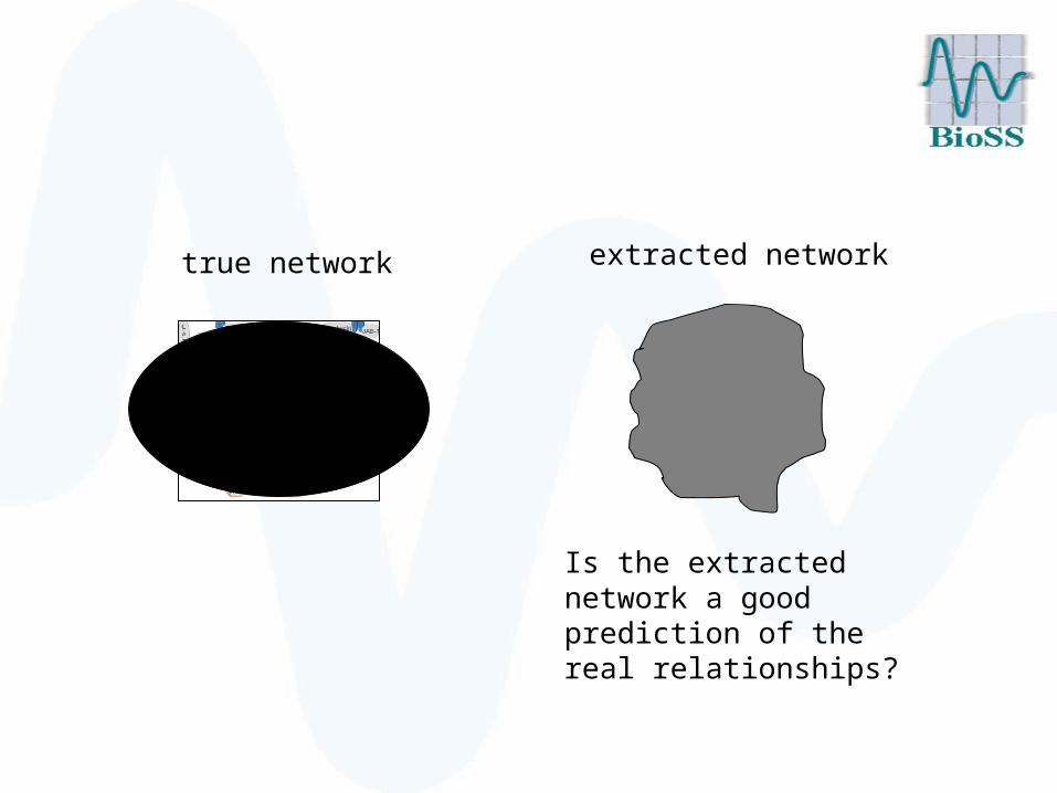
true network extracted network
Is the extracted network a good prediction of the real relationships?

true network extracted network
biological knowledge
(gold standard network)
Evaluation of
learning
performance

Reverse Engineering of Regulatory Networks
• Can we learn network structures from postgenomic data themselves?
• Are there statistical methods to distinguish between direct and indirect correlations?
• Is it worth applying time-consuming Bayesian network approaches although computationally cheaper methods are available?
• Do active interventions improve the learning performances?– Gene knockouts (VIGs, RNAi)
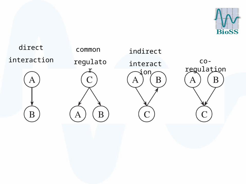
direct
interaction
common
regulator
indirect
interaction
co-regulation

Reverse Engineering of Regulatory Networks
• Can we learn network structures from postgenomic data themselves?
• Are there statistical methods to distinguish between direct and indirect correlations?
• Is it worth applying time-consuming Bayesian network approaches although computationally cheaper methods are available?
• Do active interventions improve the learning performances?– Gene knockouts (VIGs, RNAi)

• Relevance networks
• Graphical Gaussian models
• Bayesian networks
Three widely applied methodologies:

• Relevance networks
• Graphical Gaussian models
• Bayesian networks

Relevance networks(Butte and Kohane, 2000)
1. Choose a measure of association A(.,.)
2. Define a threshold value tA
3. For all pairs of domain variables (X,Y) compute their association A(X,Y)
4. Connect those variables (X,Y) by an undirected edge whose association A(X,Y) exceeds the predefined threshold value tA

Relevance networks(Butte and Kohane, 2000)

Relevance networks(Butte and Kohane, 2000)
1. Choose a measure of association A(.,.)
2. Define a threshold value tA
3. For all pairs of domain variables (X,Y) compute their association A(X,Y)
4. Connect those variables (X,Y) by an undirected edge whose association A(X,Y) exceeds the predefined threshold value tA

direct
interaction
common
regulator
indirect
interaction
co-regulation

Pairwise associations without taking the context of the
system into consideration
direct
interaction
pseudo-correlations
between A and B
E.g.:Correlation between A and C is
disturbed (weakend) by the
influence of B

1 2
X
21
X
21
‘direct interaction’
‘common regulator’
‘indirect interaction’X
21
1 2
strong
correlation σ12

• Relevance networks
• Graphical Gaussian models
• Bayesian networks

Graphical Gaussian Models
jjii
ijij
)()(
)(111
1
2
2
1
1
direct interaction
Partial correlation, i.e. correlation
conditional on all other domain variables
Corr(X1,X2|X3,…,Xn)
But usually: #observations < #variables
strong partial
correlation π12

Shrinkage estimation of the covariance matrix
(Schäfer and Strimmer, 2005)
TMLMLS T |000ˆˆ)1()|(ˆ
]||)|(ˆ[||))|(ˆ( 2FSS TETMSE
))|(ˆ())|(ˆ( 0 TMSETMSE SS with
where
0<λ0<1 estimated (optimal) shrinkage intensity,
is guaranteed0)|(ˆ0 TS
nn
TML
00
0
0
00
ˆ 22
11
|

direct
interaction
common
regulator
indirect
interaction
co-regulation

Graphical Gaussian Models
direct
interaction
common
regulator
indirect
interaction
P(A,B)=P(A)·P(B)
But: P(A,B|C)≠P(A|C)·P(B|C)

Further drawbacks
• Relevance networks and Graphical Gaussian models can extract undirected edges only.
• Bayesian networks promise to extract at least some directed edges. But can we trust in these edge directions?
It may be better to learn undirected edges than learning directed edges with false orientations.

• Relevance networks
• Graphical Gaussian models
• Bayesian networks

Bayesian networks
A
CB
D
E F
NODES
EDGES
•Marriage between graph theory and probability theory.
•Directed acyclic graph (DAG) represents conditional independence relations.
•Markov assumption leads to a factorization of the joint probability distribution:
),|()|(),|()|()|()(
),,,,,(
DCFPDEPCBDPACPABPAP
FEDCBAP

Bayesian networks versus causal networks
Bayesian networks represent conditional (in)dependency relations - not necessarily causal interactions.

Bayesian networks versus causal networks
A
CB
A
CB
True causal graph
Node A unknown

Bayesian networks
A
CB
D
E F
NODES
EDGES
•Marriage between graph theory and probability theory.
•Directed acyclic graph (DAG) represents conditional independence relations.
•Markov assumption leads to a factorization of the joint probability distribution:
),|()|(),|()|()|()(
),,,,,(
DCFPDEPCBDPACPABPAP
FEDCBAP

Bayesian networks
n
jijjijii xbNX
1
2 )),((~ ijij XXb 0
)()|()(
)()|()|( graphPgraphdataP
dataP
graphPgraphdataPdatagraphP
Parameterisation: Gaussian BGe scoring metric:
data~N(μ,Σ)
with normal-Wishart distribution of the (unknown) parameters,
i.e.:
μ~N(μ*,(vW)-1) and W~Wishart(T0)
)()|)(,()( graphdgraphgraphdataPgraphP

Bayesian networks
)()|)(,()( graphdgraphgraphdataPgraphP
)()|()(
)()|()|( graphPgraphdataP
dataP
graphPgraphdataPdatagraphP
BGe metric: closed form solution
)|( datagraphscoreBGe
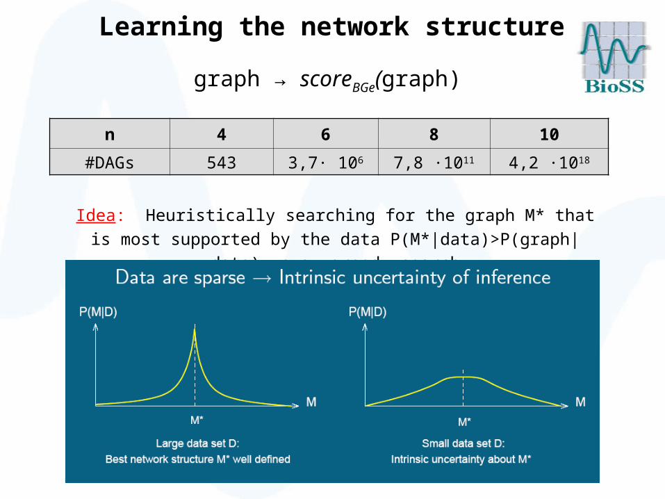
Learning the network structure
n 4 6 8 10
#DAGs 543 3,7· 106 7,8 ·1011 4,2 ·1018
Idea: Heuristically searching for the graph M* that is most supported by the data P(M*|data)>P(graph|data), e.g. greedy
search
graph → scoreBGe(graph)

MCMC sampling of Bayesian networks
• Better idea: Bayesian model averaging via Markov Chain Monte Carlo (MCMC) simulations
• Construct and simulate a Markov Chain (Mt)t in the space of DAGs {graph} whose distribution converges to the graph posterior distribution as stationary distribution, i.e.:
P(Mt=graph|data) → P(graph|data) t → ∞
to generate a DAG sample: G1,G2,G3,…GT

Order MCMC(Friedman and Koller, 2003)
• Order MCMC generates a sample of node orders from which in a second step DAGs can be sampled:
A B D E FC
A B D E FC
A F D E BC
old
new
A F D E AC → DAG
)|(
)|(,1min)|(
old
newoldnew DP
DPA
Acceptance probability (Metropolis Hastings)
G1,G2,G3,…GT
DAG sample

Equivalence classes of BNs
)|()()|(
)()|()()()|( 1
BCPBPCAP
CPCAPCPBPBCP
11 )(),()(),()(
)|()|()(
APACPCPCBPAP
ACPCBPAP
),|()()( BACPBPAP
A
B
C
A
B
A
B
A
B
C
C
C
)()|()|(
),()|(
CPCBPCAP
CBPCAP
A
B
C
completed partially directed graphs (CPDAGs)
A
C
B
v-structure
P(A,B)=P(A)·P(B)
P(A,B|C)≠P(A|C)·P(B|C)
P(A,B)≠P(A)·P(B)
P(A,B|C)=P(A|C)·P(B|C)

CPDAG representationsA
B C
D
E F
DAGs CPDAGs
Utilise the CPDAG sample for estimating the posterior probability of edge relation
features:
T
iiGIT
BAP1
)(1
)(ˆ
where I(Gi) is 1 if the CPDAG Gi contains the directed edge A→B, and 0 otherwise
A
B C
D
E F

CPDAG representationsA
B C
D
E F
A
B C
D
E F
DAGs CPDAGs
Utilise the DAG (CPDAG) sample for estimating the posterior probability of edge relation
features:
T
iiGIT
BAP1
)(1
)(ˆ
where I(Gi) is 1 if the CPDAG of Gi contains the directed edge A→B, and 0 otherwise
A
B C
D
E F
interpretation
superposition

Interventional data
A B
A B A B
inhibition of A
A B
n
iXpaiii i
DXpaDXPMDP1
][ )][|()|(
n
i
iXpai
iii i
DXpaDXP1
}{][
}{ )][|(
down-regulation of B
no effect on B
A and B are correlated

Evaluation of Performance
• Relevance networks and Graphical Gaussian models extract undirected edges (scores = (partial) correlations)
• Bayesian networks extract undirected as well as directed edges (scores = posterior probabilities of edges)
• Undirected edges can be interpreted as superposition of two directed edges with opposite direction.
• How to cross-compare the learning performances when the true regulatory network is known?
• Distinguish between DGE (directed graph evaluation) and UGE (undirected graph evaluation)

data
Probabilistic inference - DGE
true regulatory network
Thresholding
edge scores
TP:1/2
FP:0/4
TP:2/2
FP:1/4
concrete networkpredictions
lowhigh

data
Probabilistic inference - UGE
undirected edge scores
add up scores of directed edges with opposite direction
skeleton of
true regulatory network

data
Probabilistic inference - UGE
skeleton of
true regulatory network
undirected edge scores
add up scores of directed edges with opposite direction
+
++

data
Probabilistic inference
skeleton of
true regulatory network
undirected edge scores

data
Probabilistic inference
skeleton of
true regulatory network
Thresholding
undirected edge scores
TP:1/2
FP:0/1
TP:2/2
FP:1/1
high low
concrete network(skeleton) predictions

Evaluation 1: AUC scoresArea under Receiver Operator Characteristic
(ROC) curve
AUC=0.5 AUC=1 0.5<AUC≤1
sen
siti
vit
y
inverse specificity

Evaluation 2: TP scores
We set the threshold such that we obtained 5 spurious edges (5 FPs) and counted the corresponding number of true edges (TP count).
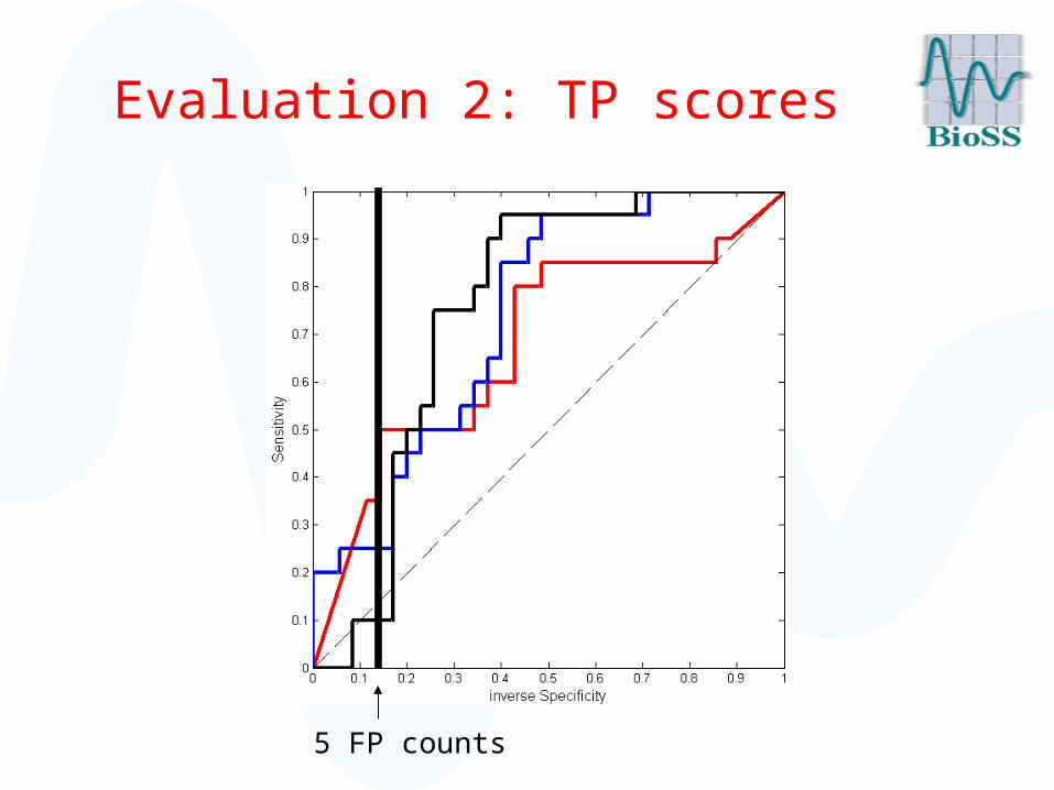
Evaluation 2: TP scores
5 FP counts

Evaluation 2: TP scores
5 FP counts
BN
GGM
RN


Evaluation
• On real experimental cytometric from the RAF signalling pathway for which a gold standard network is known
• On synthetic data simulated from this gold-standard network topology

Evaluation
• On real experimental cytometric from the RAF signalling pathway for which a gold standard network is known
• On synthetic data simulated from the gold-standard network topology

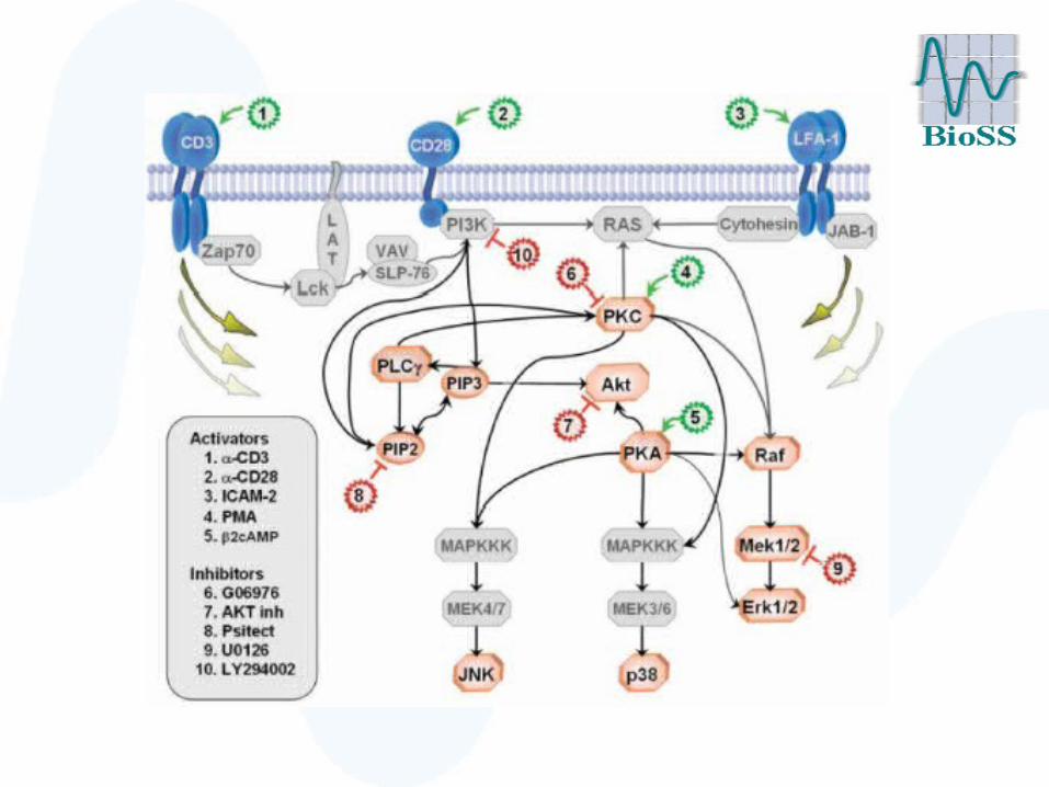
Evaluation: Raf signalling pathway
• Cellular signalling cascade which consists of 11 phosphorylated proteins and phospholipids in human immune systems cell
• Deregulation carcinogenesis
• Extensively studied in the literature gold standard network

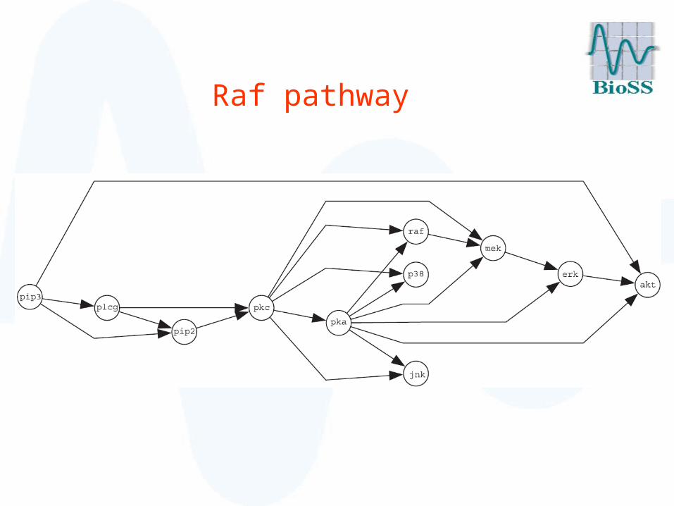
‘gold standard RAF pathway‘ according to Sachs et al. (2004)

Raf pathway
11 nodes (proteins) and 20 directed edges

Data
• Intracellular multicolour flow cytometry experiments concentrations of 11 proteins
• 5400 cells have been measured under 9 different cellular conditions (cues)
• We decided to downsample our test data sets to 100 instances - indicative of microarray experiments


Two types of experiments
Evaluation
• On real experimental data, using the gold standard network from the literature
• On synthetic data simulated from this gold-standard network

Raf pathway

Gaussian simulated data

Netbuilder simulated data
DNA + TF`s→ DNA●TF → mRNA → protein

011
mRNAkk
t
mRNA
0][Pr][
Pr22
oteinkmRNAkt
otein
)1()1(0
1
ABBAk
A
A
K
TF ][
B
B
K
TF ][
DNA + TFA DNA●TFA
DNA + TFB DNA●TFB
Netbuilder simulated data
Steady-state approximation
KA
KB

Generating data using Netbuilder tool
The main idea of Netbuilder is instead of solving the steady state approximation to ODEs explicitly, we approximate them with a qualitatively equivalent
combination of multiplications and sums of sigmoidal transfer functions.
Netbuilder simulated data

Experimental Results
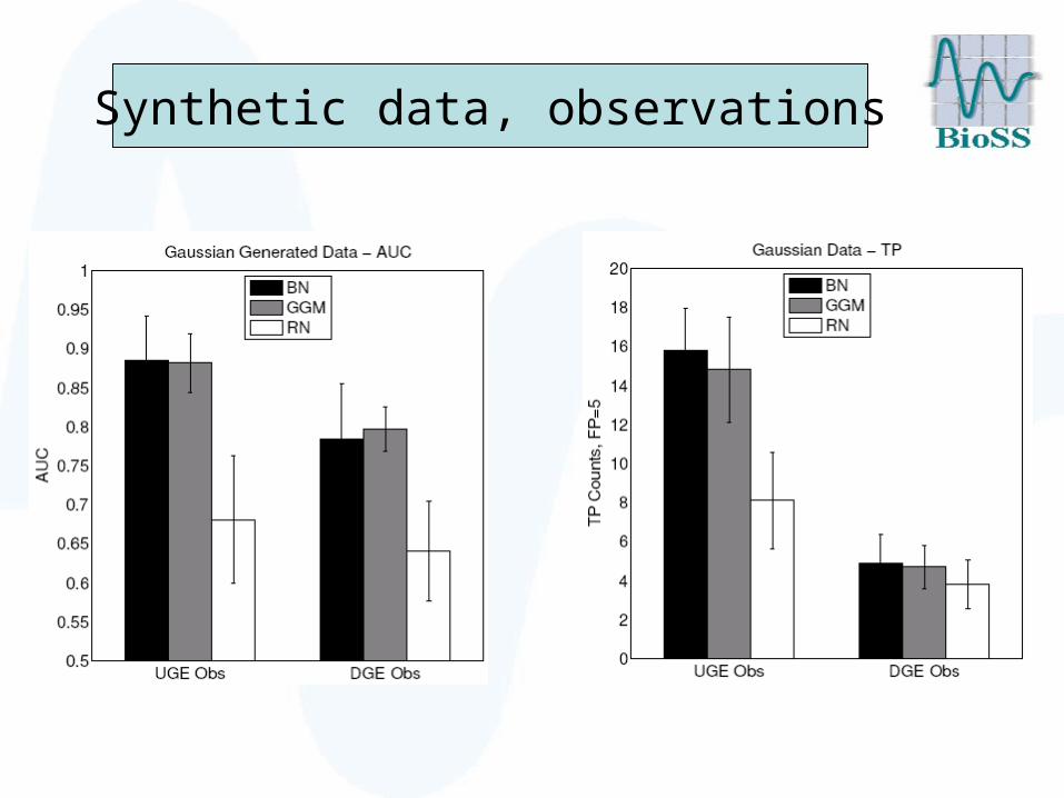
Synthetic data, observations

Synthetic data, interventions

Cytometry data, observations

Cytometry data, interventions


How can we explain the difference between synthetic
and real data ?
Raf pathway


Regulation of Raf-1 by Direct Feedback Phosphorylation. Molecular Cell, Vol. 17, 2005 Dougherty et al
Disputed structure of the gold-standard network

Complications with real data
• Interventions are not “ideal” owing to negative feedback loops.
• Putative negative feedback loops: Can we trust our gold-standard network?
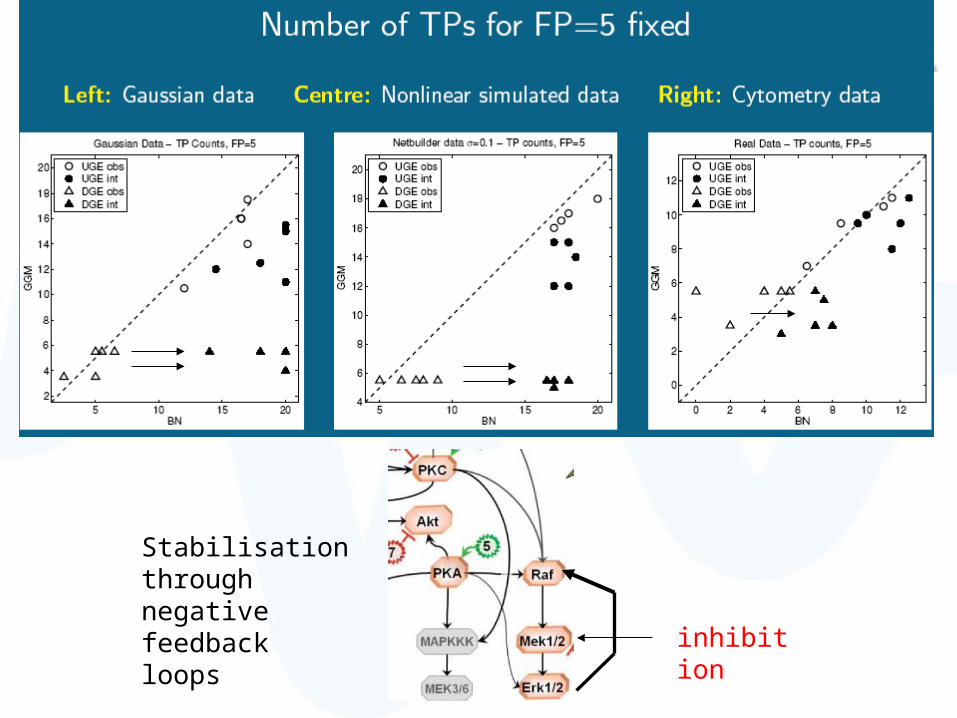
Stabilisationthrough negative feedback loops inhibition

Conclusions 1
• BNs and GGMs outperform RNs, most notably on Gaussian data.
• No significant difference between BNs and GGMs on observational data.
• For interventional data, BNs clearly outperform GGMs and RNs, especially when taking the edge direction (DGE score) rather than just the skeleton (UGE score) into account.

Conclusions 2
Performance on synthetic data better than on real data.
• Real data: more complex• Real interventions are not ideal• Errors in the gold-standard
network

Additional analysis I: Raf pathway

Additional analysis I: Raf pathway

Additional analysis I: Raf pathway

CPDAGs of networks
3/20 directed edges 13/16 directed edges
ORIGINALMODIFIED

ORIGINAL MODIFIEDG
au
ssi
an
Ne
tbu
ilde
r

Some additional analysis II

Thank you

References:
Butte, A.S. and Kohane, I.S. (2003): Relevance networks: A first step toward finding genetic regulatory networks within microarray data. In Parmigiani, G., Garett, E.S., Irizarry, R.A. und Zeger, S.L. editors, The analysisof Gene Expression Data, pages 428-446. Springer.
Doughtery, M.K. et al. (2005): Regulation of Raf-1 by Direct Feedback Phosphorylation. Molecular Cell, 17, 215-227.
Friedman, N. and Koller, D. (2003): Being Bayesian about network structure.Machine Learning, 50:95-126.
Madigan, D. and York, J. (1995): Bayesian graphical models for discrete data. International Statistical Review, 63:215-232.
Sachs, K., Perez, O., Pe`er, D., Lauffenburger, D.A., Nolan, G.P. (2004):Protein-signaling networks derived from multiparameter single-cell data. Science, 308:523-529.
Schäfer, J. and Strimmer, K. (2005): A shrinkage approach to large-scalecovariance matrix estimation and implications for functional genomics. Statistical Applications in Genetics and Molecular Biology, 4(1): Article 32.