Reverse engineering of gene regulatory networks

Reverse engineering of gene regulatory networks

K.-H. Cho, S.-M. Choo, S.H. Jung, J.-R. Kim, H.-S. Choi and J. Kim

Abstract: Systems biology is a multi-disciplinary approach to the study of the interactions ofvarious cellular mechanisms and cellular components. Owing to the development of new technol-ogies that simultaneously measure the expression of genetic information, systems biological studiesinvolving gene interactions are increasingly prominent. In this regard, reconstructing gene regulat-ory networks (GRNs) forms the basis for the dynamical analysis of gene interactions and relatedeffects on cellular control pathways. Various approaches of inferring GRNs from gene expressionprofiles and biological information, including machine learning approaches, have been reviewed,with a brief introduction of DNA microarray experiments as typical tools for measuring levelsof messenger ribonucleic acid (mRNA) expression. In particular, the inference methods are classi-fied according to the required input information, and the main idea of each method is elucidated bycomparing its advantages and disadvantages with respect to the other methods. In addition, recentdevelopments in this field are introduced and discussions on the challenges and opportunities forfuture research are provided.

1 Introduction

In order to have a better understanding on complex biologi-cal phenomena and disease mechanisms, we need to unravelthe interaction structure of molecular components involvedin the cellular processes rather than just characterising theproperties of individual components. In this paper, wefocus on gene regulatory networks (GRNs) representingthe interaction structure of genes [1]. In general, a GRN isrepresented by a directed graph composed of nodes (genes)and links (regulatory relationships). The regulatory relation-ship can be either an activation (i.e. inducing transcription ofother genes) or an inhibition (i.e. repressing transcriptionalactivity). Two nodes without a link imply that no regulatoryrelationship exists between them. Inference of such a GRNfor a specific part or the entire genome can help us tounravel the gene interaction mechanism for a particularstimulation and we can further utilise this information topredict adverse effects of new drugs or to identify a newdrug target. Owing to the development of new high-throughput measurement technologies such as DNAmicroarray, ChIP (CHromatin ImmunoPrecipitation)–chipexperiments and protein–protein interaction measurements(see Section 2), there is a renewed interest in unravellingthe hidden GRN. The inference of such a GRN from either

# The Institution of Engineering and Technology 2007

doi:10.1049/iet-syb:20060075

Paper first received 7th April 2006 and in revised form 30th January 2007

K.-H. Cho is with the College of Medicine, Seoul National University, Jongno-gu, Seoul 110-799, South Korea

S.-M. Choo is with the School of Electrical Engineering, University of Ulsan,Ulsan 680-749, South Korea

S.H. Jung is with the Department of Information and CommunicationEngineering, Hansung University, Seoul 136-792, South Korea

J.-R. Kim is with the Bio-MAX Institute, Seoul National University, Gwanak-gu, Seoul 151-818, South Korea

H.-S. Choi and J. Kim are with the Interdisciplinary Program in Bioinformatics,Seoul National University, Gwanak-gu, Seoul 151-747, South Korea

K.-H. Cho is also with the Bio-MAX Institute, Seoul National University,Gwanak-gu, Seoul 151-818, South Korea

E-mail: [email protected] (K.-H. Cho)

IET Syst. Biol., 2007, 1, (3), pp. 149–163

gene expression profiles [more precisely, messenger ribonu-cleic acid (mRNA) expression profiles] or DNA sequenceinformation is often called ‘reverse engineering’. Variousreverse engineering methods have been developed to infersuch a GRN; however, because of both experimental limit-ations and methodological complexities, a large majorityof these methods have been not so successful as there are(i) a dimensionality problem: too many genes with toofew available sampling time points, (ii) a computationalcomplexity problem: exponential complexity if a prioriinformation is unavailable for regulatory genes and (iii) anexperimental measurement problem: no guidelines for anappropriate experimental design for distinguishing directand indirect influences among genes. Hence, we need tounderstand the essential features of each method before weapply any particular method and to choose a most suitableone considering given conditions and available data. In thisrespect, we review the previously developed reverse engin-eering methods. There are some review papers on reverseengineering [2–6], but we approach in a different way. Weexplicitly classify each method depending on the requiredinput data and the inference outputs, elucidate the keyidea of each method and compare the advantages anddisadvantages.

The overall procedure of reverse engineering GRNs isillustrated in Fig. 1. We need to understand the requiredinput information of each reverse engineering method assome methods presume specific types of data producedfrom experiments having a particular design. The inputinformation for inference methods can be either geneexpression data or biological information data such asDNA sequences and annotations (see Section 4). As alarge number of gene expression levels can bemeasured sim-ultaneously using DNA microarray, we can use geneexpression data for reverse engineering of a GRN.However, there is a limitation in inferring a GRN usingonly the expression data and hence, it has been proposed tomake further use of diverse biological information. Theinference methods requiring expression data includeBoolean methods (Section 3.1), Bayesian methods (Section3.2) and regulation matrix methods (Section 3.3), and

149

those requiring biological information as well as expressiondata include the MODEM (MODule construction using geneExpression and sequence Motif) and GRAM (GeneticRegulAtory Modules) methods (Section 4).

We also note that each inference method provides us withvarious forms of the inferred GRNs. For example, somemethods only provide correlations between genes,whereas others may provide detailed regulatory relationssuch as activation and inhibition. In some cases, the regulat-ory relations are represented by probability and the inferrednetworks are represented by module regulatory networks.Hence, we need to understand what kind of inference‘output’ can be obtained from each reverse engineeringmethod in order to choose the most appropriate one for agiven purpose. In this paper, we review various reverseengineering methods in these respects and then provide auseful guide for researchers who are interested in investi-gating new reverse engineering methods.

2 DNA microarray experiments andsequence motifs

In this section, we briefly review DNA microarray exper-iments and DNA sequence motifs, both of which provideuseful input information for reverse engineering of GRNs.Further details are to be found in [7–28].

2.1 DNA microarray experiments

We can measure genome-wide gene expression through aDNA microarray experiment which is basically an extendedversion of Northern blotting [7] measuring the abundance ofmRNAs separated by electrophoresis [8–10]. A DNAmicroarray experiment is devised to simultaneouslymeasure ten to hundreds of thousands of mRNA expressionlevels of a given sample [29], whereas Northern blotting isto measure a single mRNA expression level of a selectedgene with more accuracy. The central principle of measur-ing mRNA expression levels is the base pairing betweenunknown sequences of mRNAs in sample cells andknown complementary DNA sequences of the targetgenes [i.e. A (adenine) pairs with T (thymine), and G(guanine) pairs with C (cytosine)]. There are two types ofmicroarrays: cDNA microarray and oligonucleotide micro-array [11]. The overall procedures of DNA microarrayexperiments are illustrated in Fig. 2 considering cDNAmicroarray.

As illustrated in Fig. 2, DNA microarray experiments arecomposed of multiple steps which imply several possiblenoise sources. For instance, there might be problems

Fig. 1 Schematic diagram of typical procedures for reverseengineering of GRNs

150

caused by different binding affinities depending on DNAsequences [12], physical contamination, saturation effectof each pixel depending on the laser excitation intensity[8, 13], different dye effects [14, 15] and so on. In particular,we note that the microarray data table (Fig. 2i) can bechanged depending on the definition of the representativevalue in data1 and data2 (Fig. 2h) within the same exper-iment [18]. Hence, we need to carefully design DNA micro-array experiments to minimise such potential errors and tonormalise the measured expression data by statisticallyeliminating any systematic errors [8, 12–17, 28], whichare the main topics for microarray bioinformatics butbeyond the scope of this paper.

2.2 DNA sequence motifs

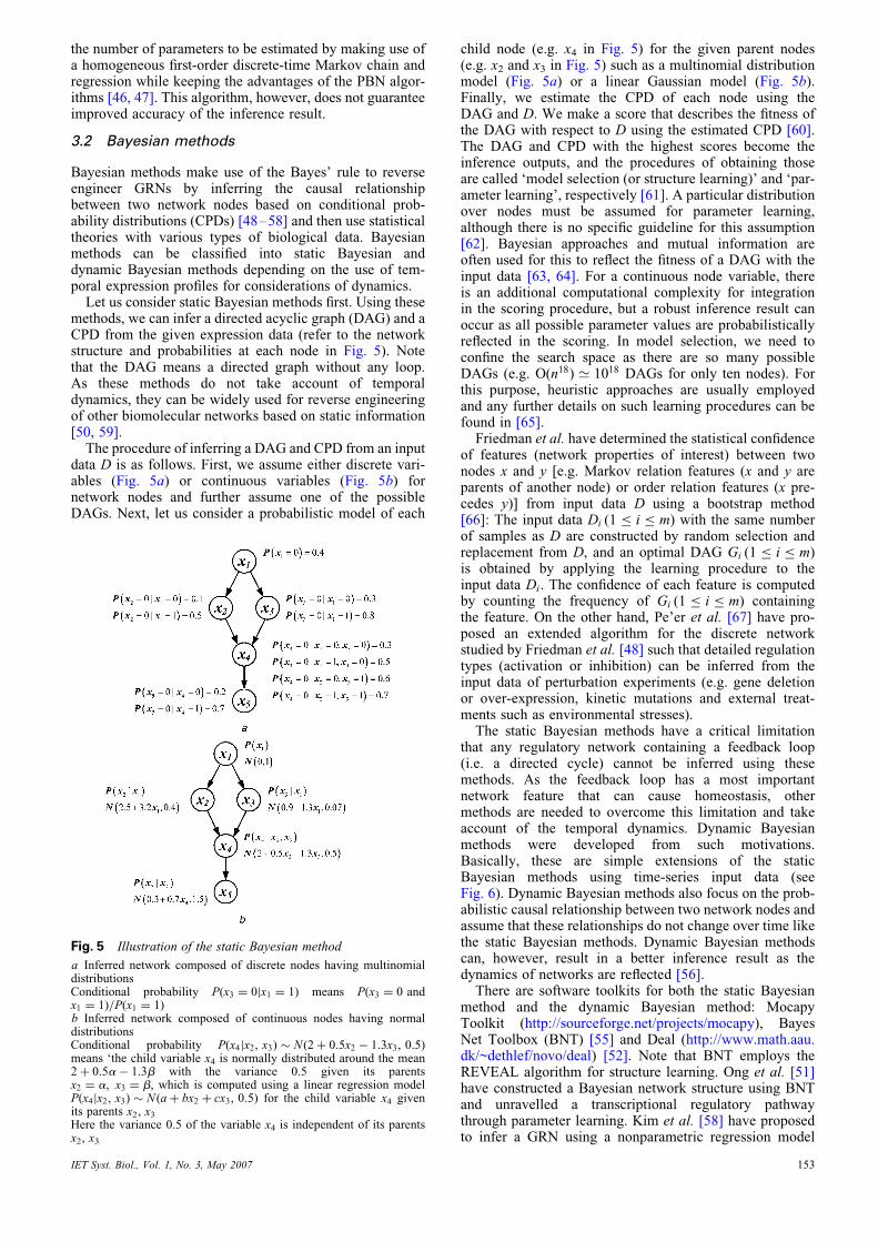
In addition to gene expression data, we can also make use ofvarious biological information for reverse engineering ofGRNs including the followings: transcription factor (TF)binding sites (sequence motifs) [19], ChIP–chip data forTF binding information based on ChIP [20], gene annota-tions [e.g. the gene annotation of SWI4 is ‘DNA bindingcomponent of SBF complex (Swi4p–Swi6p)’] [20] andprotein–protein interaction data. Such information can beused in the following processes: identification of candidategenes producing TFs, investigation of the TF binding sites[21] and search for genes in relation with the TF bindingsites [22]. We cannot, however, determine all the bindingsites of TFs through experimentation [21, 23, 24] becausethe number of TFs is exceedingly large (2000–3000 forthe human) and the genome size is also even larger (morethan 3 billion base pairs for human) [21]. As a result ofthis large scale, some in silico approaches have been devel-oped [19, 21, 25, 26]. Among them, a weight matrix method(Fig. 3) has been generally used [19, 21]; sequences knownto bind with a TF are collected (Fig. 3a) and then the distri-bution of bases at each position is computed (Fig. 3b). Theconsensus sequence of 6 bp (Fig. 3c), in which the base ateach position is the most frequent one, can be found fromthis distribution, where a TF can bind the consensussequence. However, as a TF can also bind with othersequences as seen in the experimental results of Fig. 3a,an alternate consensus sequence is also adopted (Fig. 3c).The alternate consensus sequence is the sequence permit-ting the possible plural bases at some position in the consen-sus sequence [21]. As seen in Fig. 3c, ‘GYNGAG’ can be analternate consensus sequence where N represents an arbi-trary base and Y denotes a pyrimidine (i.e. cytosine orthymine). R is conventionally employed to indicate apurine (i.e. adenine or guanine). A method of using a pos-ition weight matrix was developed (Fig. 3d) in order toevaluate how strongly a TF binds to the correspondingsequence. The weight W(b, l) of base b at lth position canbe calculated from the distribution of bases at each position(Fig. 3b) using the equation W (b, l) ¼ 10(2þ log2 f (b, l))where f(b, l) denotes the frequency of base b at lth position.This kind of in silico approach for finding a relationshipbetween TFs and genes based on only binding sites,however, still has the following two fundamental limit-ations: (i) there are too many candidate binding sites; (ii)it is not clear whether a binding site will be the cis-regulatory element (region of DNA or RNA which regulatesthe expression of genes located on that same strand) of aparticular gene. These are because the protein codingregion is relatively very small compared with the wholegenome size in many evolved complex organisms (about5% for human) or the binding site can be far away fromthe transcription initiation site and even be placed in the

IET Syst. Biol., Vol. 1, No. 3, May 2007

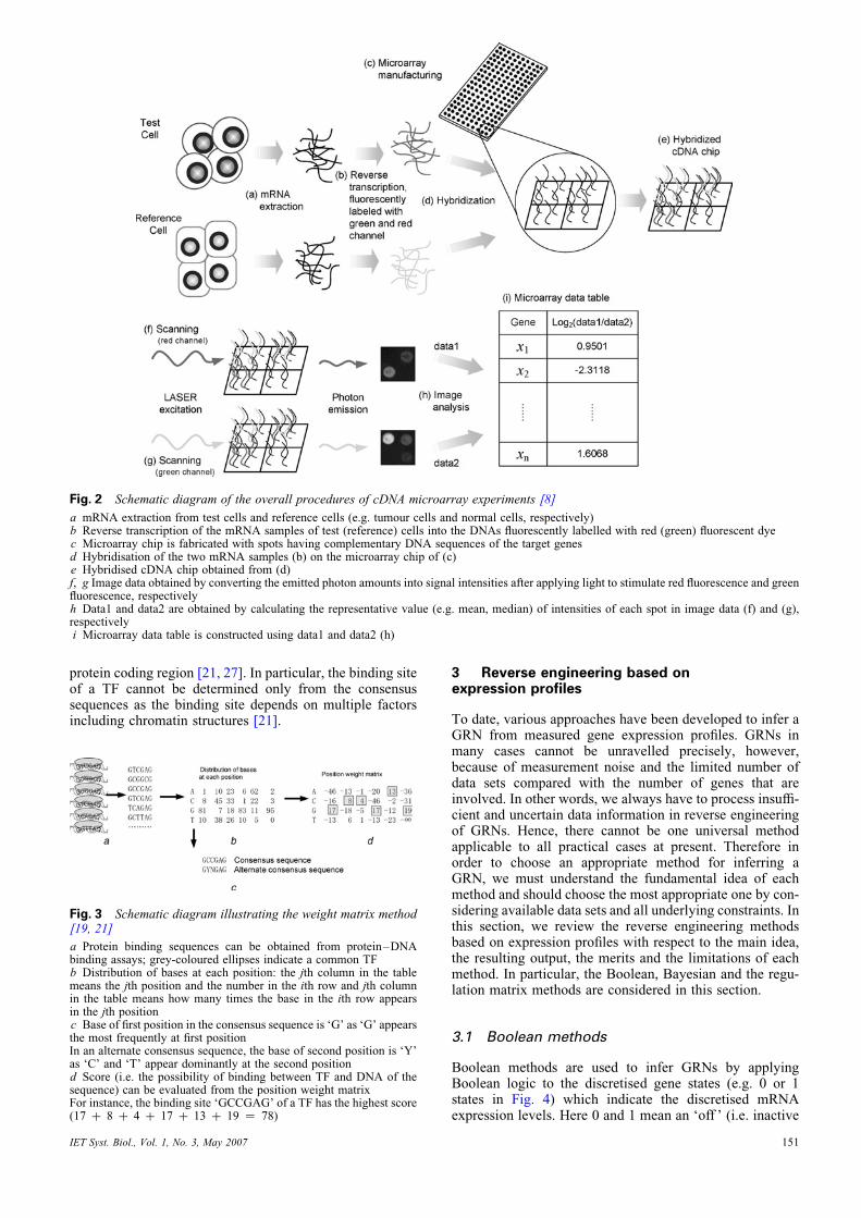
Fig. 2 Schematic diagram of the overall procedures of cDNA microarray experiments [8]

a mRNA extraction from test cells and reference cells (e.g. tumour cells and normal cells, respectively)b Reverse transcription of the mRNA samples of test (reference) cells into the DNAs fluorescently labelled with red (green) fluorescent dyec Microarray chip is fabricated with spots having complementary DNA sequences of the target genesd Hybridisation of the two mRNA samples (b) on the microarray chip of (c)e Hybridised cDNA chip obtained from (d)f, g Image data obtained by converting the emitted photon amounts into signal intensities after applying light to stimulate red fluorescence and greenfluorescence, respectivelyh Data1 and data2 are obtained by calculating the representative value (e.g. mean, median) of intensities of each spot in image data (f) and (g),respectivelyi Microarray data table is constructed using data1 and data2 (h)

protein coding region [21, 27]. In particular, the binding siteof a TF cannot be determined only from the consensussequences as the binding site depends on multiple factorsincluding chromatin structures [21].

Fig. 3 Schematic diagram illustrating the weight matrix method[19, 21]

a Protein binding sequences can be obtained from protein–DNAbinding assays; grey-coloured ellipses indicate a common TFb Distribution of bases at each position: the jth column in the tablemeans the jth position and the number in the ith row and jth columnin the table means how many times the base in the ith row appearsin the jth positionc Base of first position in the consensus sequence is ‘G’ as ‘G’ appearsthe most frequently at first positionIn an alternate consensus sequence, the base of second position is ‘Y’as ‘C’ and ‘T’ appear dominantly at the second positiond Score (i.e. the possibility of binding between TF and DNA of thesequence) can be evaluated from the position weight matrixFor instance, the binding site ‘GCCGAG’ of a TF has the highest score(17 þ 8 þ 4 þ 17 þ 13 þ 19 ¼ 78)


3 Reverse engineering based onexpression profiles

To date, various approaches have been developed to infer aGRN from measured gene expression profiles. GRNs inmany cases cannot be unravelled precisely, however,because of measurement noise and the limited number ofdata sets compared with the number of genes that areinvolved. In other words, we always have to process insuffi-cient and uncertain data information in reverse engineeringof GRNs. Hence, there cannot be one universal methodapplicable to all practical cases at present. Therefore inorder to choose an appropriate method for inferring aGRN, we must understand the fundamental idea of eachmethod and should choose the most appropriate one by con-sidering available data sets and all underlying constraints. Inthis section, we review the reverse engineering methodsbased on expression profiles with respect to the main idea,the resulting output, the merits and the limitations of eachmethod. In particular, the Boolean, Bayesian and the regu-lation matrix methods are considered in this section.

3.1 Boolean methods

Boolean methods are used to infer GRNs by applyingBoolean logic to the discretised gene states (e.g. 0 or 1states in Fig. 4) which indicate the discretised mRNAexpression levels. Here 0 and 1 mean an ‘off ’ (i.e. inactive

151

or unexpressed) state and an ‘on’ (i.e. active or expressed)state of genes, respectively. Let xi(t) be the discretisedstate of a network node xi (1 � i � n) at t and a pair oftwo lists (x1(t), . . . , xn(t)) and (x1(t þ 1), . . . , xn(t þ 1)) bea state transition pair (the first list is an input state and thesecond list is an output state) where the ith component ofan input (output) state is called the input (output) state ofxi. For instance, there exist n 2 1 state transition pairsfor data measured at n time points. Boolean methods areto find a Boolean relation (a gene regulation rule) of eachnode which explains the influence of input states on thenode and then these methods can be applied to data setsmeasured at two time points at least. In order to obtain aBoolean function or a state transition pair table of eachnode as output data (see Fig. 4b), a state transition pairtable of the network (input data for the Boolean method)is formulated by summarising these input states andoutput states (see Fig. 4a).

Discretisation of mRNA expression levels makesBoolean methods useful when there are noisy input data[30]. We lose information during the discretisation ofstates, however, which may result in unrealistic inferenceoutcomes. Moreover, we cannot always find an optimalinference result because of the computational complexitythat grows exponentially according to the number ofnetwork nodes. To deal with this problem, the maximumnumber of arguments of each Boolean function isassumed to be bounded by some constant, and variousalgorithms, such as the REVEAL, BOOL-2 [31, 32], tem-poral Boolean [33], Discrete Function Learning [34],computational algebra [35, 36] and Probabilistic BooleanNetwork (PBN) algorithms [37], have been developed.The following is a review of the characteristic propertiesof each aforementioned algorithm.

REVEAL makes use of mutual information [38] in infor-mation theory as a measure of interrelationships [33, 34,39–42]. For instance, consider a network with nodeshaving two discretised states (e.g. 0 or 1) and formulatethe state transition pair table of the network as an inputdata. And then find the k arguments whose mutual infor-mation with the node xi is identical to the self-informationof the node xi by starting from k ¼ 1. If there is no suchcase for xi then we repeat this procedure after increasing k

Fig. 4 Illustration of the input and output of Boolean methods

a State transition pair table of a network with three nodes and twostates (0 or 1)b First table is the state transition pair table of the first node x1 with anargument x2 as an output using REVEAL (REVerse EngineeringALgorithm) [39]The rest are the state transition pair tables of nodes x2 and x3, respectively

152

by 1. Finally, we can construct a state transition pair tableof each node if we find such arguments for all nodes.REVEAL has been extended to cases of multiple discretisedstates [40, 41] and has formed a basis for applying infor-mation theory to reverse engineering of GRNs. Mutualinformation has been widely employed in reverse engineer-ing of GRNs. For instance, mutual information is used inBayesian methods by incorporating REVEAL into theirpackage and a modified mutual information criterion isalso used to overcome the difficulties in network learning[43]. In addition, data transmission theory, which assertsmutual information of indirect interaction is smaller thanthat of direct interaction, is used to identify the indirectrelationships among the interrelated genes [41]. REVEALhas the disadvantage in that it requires an exhaustivesearch for all pair-wise mutual information by increasingthe indegree (the number of arguments). One way ofdealing with such a difficulty is to confine the searchspace into the set S < {xj} where S consists of k nodeshaving the highest mutual information with xi when weincrease the indegree of xi from k to k þ 1 [34].Moreover, Zheng and Kwoh [34] have extended REVEALby allowing some error ranges in consideration of noisemeasurement. Alternatively, another extension of theBoolean method by considering the values of argumentsnot only at t but also at t � 1, . . . , t � (T � 1) for a givennode at t þ 1 has been proposed [33] where T is an indexrepresenting the dependency of the algorithm on the timewindow. Other approaches developed to find Boolean func-tions using logical operations and algebraic theory insteadof mutual information have been developed [32, 35, 36].For instance, the BOOL-2 algorithm, using logical oper-ations, was proposed to deal with experimental noiseeffects by considering only the Boolean functions of nodeswhich logically explain the influence of input states on cor-responding nodes with probability of more than a threshold[31, 32]. However, this algorithm does not provide any prac-tical guideline for selecting the threshold, which is critical tothe identification results of the BOOL-2 algorithm.Laubenbacher and Stigler [35, 36] have proposed the

algorithms of searching for Boolean functions from a setof polynomial functions with discretised coefficients byapplying computational algebraic theory. They haveshown that Boolean functions can be represented by poly-nomial functions with the coefficients of 0 or 1 throughtranslation of Boolean logical operators into algebraic oper-ators (e.g. x _ y :¼ xþ yþ xy). They have then assigned toeach node a polynomial function realising the relationshipbetween the input state and the output state of each statetransition pair by employing Lagrange interpolation or theChinese Remainder Theorem [44]. They have further uti-lised the Buchberger algorithm [45] to eliminate any termof the constructed polynomial function which has 0 inputstate to obtain a final Boolean function. Hence, we canfind Boolean functions using this algebraic algorithmwithout any exhaustive search; however, this algorithm issensitive to noise because of the procedure of fitting inputstates to the output states.There are probabilistic extensions of Boolean methods by

considering many Boolean functions fi1 , fi2 , . . . , fik of eachnode xi and the probabilities with which each Boolean func-tion fij is chosen to predict the state of xi [37, 46, 47]. ThePBN algorithm [46, 47] can account for the embeddeduncertainty of data and models by allowing some errorbounds in the Boolean functions. There are, however, toomany parameters to be estimated (e.g. 22

8 ’ 1077

parameters only for eight nodes). Ching et al. [37] haveproposed an extended PBN algorithm that reduces


the number of parameters to be estimated by making use ofa homogeneous first-order discrete-time Markov chain andregression while keeping the advantages of the PBN algor-ithms [46, 47]. This algorithm, however, does not guaranteeimproved accuracy of the inference result.

3.2 Bayesian methods

Bayesian methods make use of the Bayes’ rule to reverseengineer GRNs by inferring the causal relationshipbetween two network nodes based on conditional prob-ability distributions (CPDs) [48–58] and then use statisticaltheories with various types of biological data. Bayesianmethods can be classified into static Bayesian anddynamic Bayesian methods depending on the use of tem-poral expression profiles for considerations of dynamics.Let us consider static Bayesian methods first. Using these

methods, we can infer a directed acyclic graph (DAG) and aCPD from the given expression data (refer to the networkstructure and probabilities at each node in Fig. 5). Notethat the DAG means a directed graph without any loop.As these methods do not take account of temporaldynamics, they can be widely used for reverse engineeringof other biomolecular networks based on static information[50, 59].The procedure of inferring a DAG and CPD from an input

data D is as follows. First, we assume either discrete vari-ables (Fig. 5a) or continuous variables (Fig. 5b) fornetwork nodes and further assume one of the possibleDAGs. Next, let us consider a probabilistic model of each

Fig. 5 Illustration of the static Bayesian method

a Inferred network composed of discrete nodes having multinomialdistributionsConditional probability P(x3 ¼ 0jx1 ¼ 1) means P(x3 ¼ 0 andx1 ¼ 1)=P(x1 ¼ 1)b Inferred network composed of continuous nodes having normaldistributionsConditional probability P(x4jx2, x3) � N (2þ 0:5x2 � 1:3x3, 0:5)means ‘the child variable x4 is normally distributed around the mean2þ 0:5a� 1:3b with the variance 0.5 given its parentsx2 ¼ a, x3 ¼ b, which is computed using a linear regression modelP(x4jx2, x3) � N (aþ bx2 þ cx3, 0:5) for the child variable x4 givenits parents x2, x3Here the variance 0.5 of the variable x4 is independent of its parentsx2, x3


child node (e.g. x4 in Fig. 5) for the given parent nodes(e.g. x2 and x3 in Fig. 5) such as a multinomial distributionmodel (Fig. 5a) or a linear Gaussian model (Fig. 5b).Finally, we estimate the CPD of each node using theDAG and D. We make a score that describes the fitness ofthe DAG with respect to D using the estimated CPD [60].The DAG and CPD with the highest scores become theinference outputs, and the procedures of obtaining thoseare called ‘model selection (or structure learning)’ and ‘par-ameter learning’, respectively [61]. A particular distributionover nodes must be assumed for parameter learning,although there is no specific guideline for this assumption[62]. Bayesian approaches and mutual information areoften used for this to reflect the fitness of a DAG with theinput data [63, 64]. For a continuous node variable, thereis an additional computational complexity for integrationin the scoring procedure, but a robust inference result canoccur as all possible parameter values are probabilisticallyreflected in the scoring. In model selection, we need toconfine the search space as there are so many possibleDAGs (e.g. O(n18) ’ 1018 DAGs for only ten nodes). Forthis purpose, heuristic approaches are usually employedand any further details on such learning procedures can befound in [65].

Friedman et al. have determined the statistical confidenceof features (network properties of interest) between twonodes x and y [e.g. Markov relation features (x and y areparents of another node) or order relation features (x pre-cedes y)] from input data D using a bootstrap method[66]: The input data Di (1 � i � m) with the same numberof samples as D are constructed by random selection andreplacement from D, and an optimal DAG Gi (1 � i � m)is obtained by applying the learning procedure to theinput data Di. The confidence of each feature is computedby counting the frequency of Gi (1 � i � m) containingthe feature. On the other hand, Pe’er et al. [67] have pro-posed an extended algorithm for the discrete networkstudied by Friedman et al. [48] such that detailed regulationtypes (activation or inhibition) can be inferred from theinput data of perturbation experiments (e.g. gene deletionor over-expression, kinetic mutations and external treat-ments such as environmental stresses).

The static Bayesian methods have a critical limitationthat any regulatory network containing a feedback loop(i.e. a directed cycle) cannot be inferred using thesemethods. As the feedback loop has a most importantnetwork feature that can cause homeostasis, othermethods are needed to overcome this limitation and takeaccount of the temporal dynamics. Dynamic Bayesianmethods were developed from such motivations.Basically, these are simple extensions of the staticBayesian methods using time-series input data (seeFig. 6). Dynamic Bayesian methods also focus on the prob-abilistic causal relationship between two network nodes andassume that these relationships do not change over time likethe static Bayesian methods. Dynamic Bayesian methodscan, however, result in a better inference result as thedynamics of networks are reflected [56].

There are software toolkits for both the static Bayesianmethod and the dynamic Bayesian method: MocapyToolkit (http://sourceforge.net/projects/mocapy), BayesNet Toolbox (BNT) [55] and Deal (http://www.math.aau.dk/~dethlef/novo/deal) [52]. Note that BNT employs theREVEAL algorithm for structure learning. Ong et al. [51]have constructed a Bayesian network structure using BNTand unravelled a transcriptional regulatory pathwaythrough parameter learning. Kim et al. [58] have proposedto infer a GRN using a nonparametric regression model

153

http://sourceforge.net/projects/mocapy

http://www.math.aau.dk/~dethlef/novo/deal

http://www.math.aau.dk/~dethlef/novo/deal

Fig. 6 Illustration of the dynamic Bayesian method

a Cyclic regulatory network with three nodesb Microarray time-series data produced from (a)c First-order Markov relations with Xi ¼ (x1(ti), x2(ti), x3(ti)) and t1 , t2 , t3 , t4d The network structure and the CPD of each node are assumed to be time-invariante Transition network representing the causal relationship between Xi and Xiþ1, which is to be learned [64]

and employing the dynamic Bayesian algorithm. Yu et al.[57] have proposed an influence scoring to infer detailedregulatory types (activation or inhibition) and the relativemagnitude of node interactions. They have further shownthat the combination of the Bayesian Dirichlet equivalence(BDe) scoring metric based on Bayesian posteriori prob-ability [68] and a greedy search algorithm results in bestinference outputs among the combinations of the variousscoring metrics (e.g. BDe, Bayesian information criterion)and search algorithms (e.g. greedy algorithm with randomrestarts, simulated annealing, genetic algorithm). Li andChan [53] have reported that they have successfully inferredsome subnetworks such as tricarboxylic acid and ureacycles by combining several Bayesian methods. Recently,Zou and Conzen [54] have investigated a new dynamicBayesian algorithm in consideration of time-lag effects.

3.3 Regulation matrix methods

In general, a GRN can be represented by an ordinary differ-ential equation d x(t)=dt ¼ f (x(t)) or a discrete-timeequation x(t þ 1) ¼ f (x(t)), where x(t) ¼ (x1(t), . . . , xn(t))is a vector of nodes xi (1 � i � n) representing geneexpression levels at time t and f ¼ (f1, . . . , fn) is a vector-valued function from the real n-dimensional space Rn intoRn. The function f can be a linear [69–73], piecewiselinear [2, 74], pseudo-linear (i.e. composite function of asigmoid function and a linear function) [75, 76] or continu-ous (differentiable) nonlinear function such as a power-lawfunction represented by S-systems [77]. Detailed descrip-tions of various models can be found in [2, 78]. Note thatthe discrete-time equation corresponds to the Booleanmodel if f takes its value from {0,1}n. There was alsoanother development employing partial differentialequations to describe the spatial location [2]. As most bio-molecular networks, in general, have nonlinear dynamics,we should consider nonlinear models, but this causesmuch more difficulties in estimating parameters from thelimited number of data samples. This is the reason whyno effective inference method has been suggested yet insuch direction and many reverse engineering methodsinfer the regulatory relationship by solving a linear (moreexactly, linearised) system instead of directly inferring thenonlinear function f. Hence, in this section, we focus onthose methods based on linear systems, categorised as regu-lation matrix methods. In regulation matrix methods, we

154

want to find a solution A ¼ (aij) of the linearsystem ~yi ¼ bi þ

Pnj¼1 aij ~xj (1 � i � n) derived from

dx(t)=dt ¼ f (x(t)) or x(t þ 1) ¼ f (x(t)). Here bi, ~xi and ~yiare directly computed from experimental data (~xi and ~yican have various forms; see Sections 3.3.1 and 3.3.2), andaij denotes @fi=@xj or (@fi=@xj)=(� @fi=@xi) which are theregulatory relationships of xi on xj (i.e. @(dxi=d t)=@xj or@xi=@xj ). Thus, if aij . 0, xj activates xi by enhancing(the net rate of) the production of xi; if aij , 0, xj inhibitsxi by reducing (the net rate of) the production of xi andaij ¼ 0 implies that xj has no regulatory relation on xi. Inthis respect, the matrix A is called a regulation matrix(see Sections 3.3.1 and 3.3.2).Although the Boolean method assumes discretised

expression levels, regulation matrix methods directlymake use of continuous expression levels without loss ofany information caused by discretisation. Moreover, con-trary to the Bayesian methods, which are based on probabil-istic concepts, regulation matrix methods do not rely onsuch probabilistic notions, but instead make use of linearalgebra such as linear regression, principal componentsanalysis, singular value decomposition (SVD), Gaussianelimination and so on. This means that regulation matrixmethods can infer GRNs in a more quantitative mannerthan the Boolean methods if proper data measurementsare conducted. Using regulation matrix methods, we canalso estimate the strength of interactions. On the otherhand, if given data contain many noises, regulation matrixmethods might result in poor inference results comparedwith the Boolean and Bayesian methods. Regulationmatrix methods can be further classified according to therequired data types: steady-state or time-series expressiondata (see Fig. 7 for an overall sketch).

3.3.1 Regulation matrix methods based onsteady-state data: Regulation matrix methods basicallyutilise the linear system ~yi ¼ bi þ

Pnj¼1 aij ~xj (1 � i � n)

around a steady state. In general, steady-state measurementsof gene expression levels are required before/after geneperturbations such as variations of temperature, pH andusing plasmids. In some cases, parameters that indirectlyinfluence a set of particular genes are perturbed instead ofdirect gene perturbations. We need to design a sophisticatedperturbation experiment so that the characteristics of a GRNare well reflected in the steady-state data because it isimpossible to infer the interaction relationships from a


Fig. 7 Illustration of the regulation matrix methods based on either steady-state expression data or time-series data

single sampling at the steady state. We also note that theperturbation amounts can be critical because too large vari-ations cannot be used for linearised models.Several methods have been suggested to solve this linear

equations using steady-state data and to obtain the regu-lation matrix A under different circumstances [72, 79–86](see Fig. 8).Yeung et al. [87] have proposed a method of utilising the

estimate of d(xi � xsi )=dt obtained from linear interpolationwithout assuming d(xi � xsi )=dt ¼ 0. They have computedthe regulation matrix by employing SVD [71, 88] to decom-pose the data matrix and regression to identify the sparsestnetwork (Fig. 8c) [89]. Gardner et al. [72] have made use ofthe sparseness of a regulation matrix and assumed that themaximal number of nonzero elements at each row of A isk (the upper bound of the indegree of a gene). On thebasis of this assumption, they reduced the number of vari-ables to estimate from n2 into kn. In other words, they con-verted the problem into an over-determined one andcomputed A using the multiple linear regression (Fig. 8d).An example of a small network composed of nine genesrelated to the SOS pathway was used for illustration ofthis method based on perturbation experiments with quanti-tative polymerase chain reaction. Tegner et al. [82] havedeveloped an algorithm for determining the least numberof genes to be perturbed and applied the algorithm to thepreviously described method. Di Bernardo et al. [81] havealso employed the ‘Forw-TopD-reest-K’ search algorithm[90] for reverse engineering of large-scale networks. Thebasic idea is to choose D optimal solutions for k ¼ 1 andextend these solution networks by adding other connections(one by one) for each incremental change of k and choosethe solution with the smallest error for k ¼ K.The aforementioned methods have a common difficulty of

estimating the perturbation amount from the measured dataafter perturbation. To handle this difficulty, Kholodenkoet al. [79] proposed another type of perturbation method –perturbing the parameters that indirectly affect the activityof some modules or sets of genes in a network. They haveassumed a GRN that can be decomposed into modulesxi (1 � i � n) and a corresponding parameter pk (k = i),and proposed a method of inferring aij (i = j) which satis-fies Dx s

i,k=xsi (pk) ¼

P1� j�N , j=i aijD x s

j,k=xsj ( pk) (1 � k � n,

k = i) based on steady-state data x si (pk) (before pertur-bation) and x si (pk þ Dpk) (after perturbation) whereDx s

i,k ¼ x si (pk þ Dpk)� x si (pk) (Fig. 8e). This method hasadvantages in that the amount of perturbation does notneed to be measured and a subnetwork structure affectingonly selected modules of interest can be inferred.This method, however, requires a priori information on


parameters that indirectly affect each module and does nottake any experimental noise into consideration. Comparedto the previous methods of constraining the upper bound ofindegree k [72, 81, 82], this method cannot be applied to alarge-scale network as we need to perturb as many par-ameters as the number of network nodes. A similar methodwas developed for metabolic control analysis [83, 91] andAndrec et al. [84] have extended the foregoing method ofKholodenko et al. [79] by considering experimental noiseunder a normal distribution. They have not applied,however, this method to authentic experimental data.

3.3.2 Regulation matrix methods based on time-series data: The steady-state data obtained after pertur-bation does not usually reflect the dynamical characteristicsof the gene regulatory system, but we can capture thesecharacteristics through time-series data. To make use ofsuch time-series data for reverse engineering of GRNs, wecompute the regulation matrix over these time-series data.

Assuming a GRN model of x(t þ 1) ¼ Ax(t), we willreview the methods of computing A [71, 92–94]. vanSomeren et al. [92] have proposed a method scaling downthe plausible solution network space by preprocessing theexpression data and clustering them, where preprocessingmeans thresholding (i.e. choosing only the genes with sig-nificant variations) and normalisation of the data. After pre-processing the data, they have reduced the size of a networkto be inferred by clustering the genes with Euclidean dis-tance, and hence converted the under-determined problemof finding the solution A of x(t þ 1) ¼ Ax(t) into an over-determined problem. In this way, they have inferred thenetwork of the prototypes (i.e. representatives) of the clus-ters (Fig. 8f). This method overcame the dimensionalityproblem which means a difficulty (under-determinedproblem) in reverse engineering GRNs because of thelarge scale of the networks with a little data, but it canonly reveal the regulatory network among those prototypeclusters and not between individual genes.

Next, let us assume a GRN model of x(t) ¼ Ax(t) and con-sider those methods of computing A from time-series data[69–71, 73, 75, 76, 95–98]. Chen et al. [69] assumed aGRN model of r(t) ¼ Cp(t)� Vr(t), p(t) ¼ Lr(t)� Up(t)and represented the inferred GRN as x(t) ¼ Ax(t),x ¼ (r, p) where r and p denote the concentration vectorsof mRNA and protein, respectively. They employed anapproximated difference equation and made use of the sparse-ness of GRNs to compute the regulation matrix A. They alsosuggested a method to compute C using the Fourier transformfor stable systems. This method infers a GRN in considerationof both transcription and translation using the concentration

155

Fig. 8 Illustrative examples of the regulation matrix methods

a Graph of the artificial networkb Mathematical model to generate input data with H ¼ 2, V1 ¼ V2 ¼ V3 ¼ V4 ¼ 1: bi (1 � i � 4) are detailed in the description of each methodjth Entry xsj of the column vector x5 is the measured expression level of the node xj before perturbationsc Yeung et al.’s [87] method: the jth entry of the ith column vector of X is the measured expression level of the node xj at t ¼ 2 after the perturbationof (b1, b2, b3, b4) which corresponds to the ith column vector of B (1 � i � 3, 1 � j � 4)In this method, ~yi and ~xj represent d(xi(t)� xsi )=dt and xj(t)� xsj , respectivelyDerivatives are calculated using the mean ratios of changesd Gardner et al.’s [72] method: the jth entry of the ith column vector of X is the measured steady-state expression level of the node xj at t ¼ 100 afterthe perturbation of (b1, b2, b3, b4) which corresponds to the ith column vector of B (1 � i, j � 4)In this method, ~yi and ~xj represent d(xi(t)� xsi )=dt and xj(t)� xsj , respectivelye Kholodenko et al.’s [79] method: the jth entry of the ith column vector of X is the measured steady-state expression level of the node xj at t ¼ 100after the parameter perturbation Vi ¼ 1:2 (1 � i,j � 4)In the method, Dx si,k denotes the difference of xsi (pk þ Dpk)� xsi (pk)All the other notations are detailed in the main textIn (d) and (e), we used four times bigger perturbations to infer the network and thereby we could correctly infer the network using the methodsf van Someren et al.’s [92] method: the jth entry of the ith column vector Xi of X is the expression level of the node xj at t ¼ 0:1 (i� 1) after theperturbation (b1, b2, b3, b4) ¼ (0:5, 0:5, 0:5, 0:5) (1 � i � 5, 1 � j � 4)In (c)–(f), we used 0.1 as the threshold for significant relations

profiles of both proteins and mRNAs as input data. Thismethod was proposed at the early stage of a GRN studiesand was based on differential equation models. But thismethod lacks detailed information on experimental designsuch as sampling time intervals. There is an extension ofthis method which considers time delays in x(t) ¼ Ax(t)[95]. Another extension has been made by considering a non-linear model x(t) ¼ f (x(t)) with a specific form of f(x) andintroducing a genetic algorithm for parameter estimation [76].

The aforementioned methods have assumed time-invariant regulatory relationships among genes as they

156

have used the linear system near steady states (i.e. the regu-lation matrix A has been assumed as a constant). Sontaget al. [99] have relaxed this assumption and proposeda method of inferring the regulation matrix A(t) ateach time t. They have assumed a GRN model of_xi(t) ¼ fi(x(t), p) (1 � i � n) where p is a set of parameters,and developed a method of inferring A(t) ¼ (aij(t))by making use of the time-series data xj(t, pik ),xj(t, pik þ Dpik ) (1 � j � n) measured before and after,respectively, the perturbation of a specific parameterpik (1 � k � n) that indirectly affects a node xi. In this case,


aij(t) denotes the solution of the linear system (Ripik(t þ Dt)�

Ripik(t))=Dt ¼

P1�j�N aij(t)Rjpik

(t) (1 � k � n) withRjpik

(t) ¼ xj(t, pik þ Dpik )� xj(t, pik ). This method does notrequire a small perturbation as it is not based on a linearisedmodel near steady states. Moreover, it does not requiremeasuring the perturbation amount Dpik and can be appliedto reverse engineering of a subnetwork around a specificmodule of interest as the method of Kholodenko et al. [79].Furthermore, this method provides the information on tem-poral variation of regulatory relationships. This method,however, also requires as many parameter perturbations asthe number of network nodes and therefore cannot beapplied to reverse engineering of a large-scale network.Cho et al. [100] have expounded on the fundamental con-cepts of the methods proposed by Kholodenko et al. [79]and Sontag et al. [99], and presented a comprehensiveunified framework. The basic idea was that n independentequations are required to uniquely solve the system with nunknowns, and these n linearly independent equations canbe obtained by a properly chosen set of n parameter pertur-bations. Cho et al. [101], however, have also proposed avery simple but effective reverse engineering method basedon the temporal ascending or descending slope informationfromgiven time-seriesmeasurements instead of computationthrough the measured absolute values.

4 Reverse engineering based on both geneexpression profiles and biological information

In the previous section, we reviewed the reverse engineer-ing methods that use only expression profiles and exposedthe fundamental limitations to such methods related todimensionality, computational complexities and data uncer-tainties. Hence, for better inference results, it is necessary toadopt additional information processes. In this regard, thissection will review the reverse engineering methods basednot only on expression profiles, but also on available bio-logical information such as a TF binding DNA sequence(a sequence motif shortly mentioned), which is a 50

upstream sequence of genes recognised by a common TF,gene function annotations (e.g. gene lacZ encodes protein b-galactosidase) [63], ChIP–chip data [102] and protein–protein interaction data (see Input data in Fig. 9). We canalso acquire various inference outputs by integrating thesedifferent types of biological information.There have been extensive studies on reverse engineering

of GRNs by finding sequence motifs. Tavazoie et al. [103]have applied k-means clustering algorithm (a populartechnique for clustering given data into k partitions) tocell-cycle time-series data and investigated the clusters ofsimilarly expressed genes under a particular growth con-dition. They identified the function and the sequencemotif of the genes within the same cluster using the MIPS


(Munich Information Center for Protein Sequence) categoryand the AlignACE (Aligns Nucleic Acid ConservedElements) program [104], respectively, and then found thetranscriptional sub-network regulated by the known TFrecognising this sequence motif. It is difficult to correctlyidentify the whole set of regulators of genes only fromidentification of the sequence motif of these genes as wecannot determine the chromatin modification based onlyon sequence information. Moreover, this method cannotexplain the combinatorial regulation of TFs. To solve thisproblem, we need the information based on which we canchoose sequence motifs involved in combinatorial regu-lation. To obtain the information, Beer and Tavazoie[105] have employed time-series data and diverse biologicalinformation as input data: upstream DNA sequences of800 bp of genes in the 50 direction, the space between twosequence motifs, the distance between a sequence motifand ATG (the starting point of genes), the orientation ofgenes (the right direction or the left direction of genes inthe gene map) and the order of the genes in the chromo-somes. As a result, they were able to explain the combina-torial regulation through clustering and inference of therelations between sequence motifs and gene expressionpatterns.

There also have been attempts to infer a GRN by identify-ing regulators and the relationships of these regulators thatcontrol the mRNA expression levels. Segal et al. [106] havedetermined the set of the triples (a module, a set of regula-tors and a regulation tree) using a Bayesian score [65] wherea module is a set of functionally coherent genes, regulatorsare the controllers of the module and a regulation tree is atree composed of regulators for its nodes. The input dataare mRNA expression data and candidate regulatory genes(known and putative TFs and signal transduction mol-ecules). To analyse the biological meaning of the obtainedtriples, each triple was tested for enrichment of the sequencemotifs and gene annotations. They have applied the methodto the following input data: a set of 173 Saccharomyces cer-evisiae gene expression microarrays data and candidate reg-ulator genes based on the Saccharomyces Genome Databaseand Yeast Proteome Database. Using this approach, wecan infer which modules are regulated under whatstress conditions and can further determine the genes thatregulate a specific process under a given condition ofexperiments.

The aforementioned clustering-based methods can,however, result in many false-positives because of indirectinfluences included during clustering similarly expressedgenes and searching sequence motifs. To overcome suchdifficulty, a genome-wide location analysis based onChIP–chip data [102] has been proposed to identify allpossible target genes that can bind a given TF [102, 107–115]. Bar-Joseph et al. [107] have proposed the following

Fig. 9 Reverse engineering methods based on biological information

157

GRAM algorithm using protein–DNA binding data andmRNA expression data as input data: First, all possiblecombinations of transcriptional regulators are constructedusing the binding data. Although there are potentially anexponential number of combinations, the combinations ofinterest are quite limited. This is because GRAM selects agene g and then chooses the combinations T1, . . . , Tk oftranscriptional regulators which bind to the selected geneg. Next, for each Ti, GRAM finds a collection Ci of genesto which all the transcriptional regulators in Ti commonlybinds. Then, GRAM finds a gene ci in Ci that have a‘core’ expression profile and construct a set S of genes inCi which show highly correlated expressions with ci.Through relaxation of the binding criterion, GRAM ident-ifies additional genes which are similarly expressed withci and to which all the transcriptional regulators in Ti com-monly bind. GRAM extends S by adding similarlyexpressed genes. A module Mi can be obtained by such arepeated extension through relaxation and the function ofMi can be categorised by MIPS. GRAM chooses again agene which is not included in

S1�i�k Mi and repeat the pre-

vious steps. In order to accurately identify the binding siteof a TF, however, the ChIP–chip data must be obtainedusing the activated TF [109]. An extension of this methodinvolves multivariate regression techniques to estimate thebinding affinity of each TF at a promoter (the region recog-nised by RNA polymerase for the gene transcription). Thisextension infers target regulatory genes through the corre-lation between this binding affinity and gene expression pro-files [108] and also through the correlation between DNAbinding profiles and gene expression patterns [116].

Most of the previous studies on searching target genesregulated by a TF are based on the clustering of expressiondata [102, 103, 105–108, 110–115, 117–120]. Thesemethods cannot be applied to the expression data measuredat only one time point. Moreover, we note that many geneshaving the sequence motif recognised by a TF are not directtarget genes of the TF. To handle these problems, Wanget al. [109] have proposed another method (MODEM algor-ithm) with the input data: a ChIP–chip data or TF pertur-bation experimental data measured at only one time point,a core motif (a sequence motif of about 6–8 bp length)recognised by the TF and promoter sequences of genes.An extended core motif of 12 bp was obtained from aposition-specific frequency matrix. On the basis of thejoint probability of the extended core motif and the

Fig. 10 Overview of reverse engineering of GRNs by GAs

158

expression data, they computed the probability of a genebeing a target gene of the TF. This method is advantageoususing single time point data from a single experiment andalso not requiring clustering to look for target genes.Moreover, we can search the overlapped part in severalsequence motifs using the extended motif and therebyalso reveal that several TFs work competitively in thesame sequence motif. This method, however, still cannotdistinguish direct and indirect target genes even thoughthey have used sequence motifs as the procedure offinding sequence motifs depends on expression valuesmeasured at one time point.GRNs are complicated, and experimental data sets have

intrinsic errors and diverse biological information. Thus,in order to handle the errors and use the diverse biologicalinformation, it is necessary to integrate various types of bio-logical data [59, 121–123]. In this regard, Lee et al. [59]made use of various heterogeneous functional genomicsdata: mRNA expression data (Stanford MicroarrayDatabase), gene context data [Rosetta stone data (gene-fusion data), phylogenetic profiles], experimental protein–protein interaction data (database of interacting proteins,mass spectrometry, yeast two-hybrid assay, syntheticlethal assay data), literature minig data (Medline abstracts)and five benchmark sets (Kyoto-based KEGG database,Gene Ontology annotation, the cluster orthologous groupannotation, the yeast protein localisation data generatedfrom genome-wide GFP-tagging and microscopy, MIPS).They have obtained a S. cerevisiae network consisting ofgene–gene linkages with scores (e.g. a linkage betweenopen reading frame (ORF) YLR206W and ORFYLR290C with a log likelihood score 8.826), where bench-mark sets were used to test the correct assignment of lin-kages. Only some links represented direct protein–proteininteraction and the other linkages represented probabilisticfunctional associations. The score of each linkagewas calculated with respect to four categories (co-expression, co-citation, protein sequence comparison,protein interaction) based on the Bayesian approach.Using these scores, each linkage has been assigned ascore through a unified scoring scheme. Higher scoresmean more confident linkages. We can incorporate new bio-logical information to increase the confidence of linkagesthrough this approach.

5 Machine learning approaches

In contrast to the previous methods based on logical analy-sis or mathematical developments, this section reviews thereverse engineering methods employing machine learningtechniques such as genetic algorithms, genetic program-ming, neural networks and fuzzy logic. Machine learningtechniques have been used not only for inference algor-ithms [75, 124–132], but also for the clustering ofgene expression data [133–136] and the modelling ofGRNs [137, 138]. Of particular importance, genetic algor-ithms (GAs) and genetic programming (GP) havebeen widely used to reconstruct GRNs and the clusteringof gene expression data, whereas neural networks(NNs) have often been used for modelling GRNs.Recently, NNs and fuzzy logic algorithms were fused toform a cooperative framework for the inference of GRNs[135, 136].In GA-based inference methods, we assume that a GRN

is represented by a mathematical model whose parametersare to be estimated from gene expression data using GAs.The estimation of model parameters is achieved by evol-ution of the chromosomes in a population pool. GAs have


been typically used for this evolutionary procedure as theyare widely known as robust and systematic optimisationtools applicable to general scientific and engineering pro-blems [139–141]. GAs evolve the chromosomes (in thisapplication, candidate GRNs) by means of evaluatingtheir fitness, selecting parents for a next generation anddoing crossover as well as mutation operations. Thereforeif any types of problems are represented by chromosomes(typically, represented by bit strings), GAs can efficientlyfind a (sub)optimal solution within predefined generations.Owing to this feature, GAs have mainly been applied tofunctional or combinatorial optimisation problems (e.g. bitpattern matching problems) and parameter estimation pro-blems. In parameter estimation problems, the parametersare encoded to chromosomes, and GAs find the optimal esti-mates by evolving the chromosomes in a population poolwithin a predefined resolution depending on the encodingscheme. Wahde and Hertz [75] and Repsilber et al. [124]have used GAs to estimate the parameters of GRN modelsfrom both artificial and experimental microarray data. Ibaand Mimura [132] also employed GAs to reconstructGRNs from time-series gene expression data, and in par-ticular, introduced an exon (an active link that can haveany value) and an intron (an inactive link fixed to zero) inencoding chromosomes of GAs. The number of exons waslimited to approximately 5 for each population pool (theymaintained several population pools depending on the con-straints of the exons and introns) to achieve better estimatesin a rapid manner. Their methods also provided an interac-tive platform to infer GRNs through human interventionunder graphic user interface environments. Similarmethods have been developed with different modelling fra-meworks of GRNs [125–128].Fig. 10 illustrates an overview of reverse engineering of

GRNs through parameter estimation of GAs. In Fig. 10,experimental gene expression data obtained from DNAmicroarray experiments are presented as input data. Thechromosomes of GAs in a population pool encode the par-ameters of a GRN model. The network model can be one ofthe Boolean networks [31], linear networks [71, 92–94],Bayesian networks [48], differential equations [69] andrecurrent NNs [75, 142, 143]. Any other types of networkmodels can also be applied if their parameters can beencoded into chromosomes. But the recent works [75]have mainly focused on the recurrent NN models. Likethe other applications of GAs, there are no other constraintson the network models.The initial values of encoded parameters are set to

random numbers or predefined values from a priori knowl-edge. Note that each chromosome in the population poolrepresents one candidate GRN that can be obtained bydecoding the chromosome. This candidate GRN producesa simulated gene expression data set and the GA usesthese data to score the fitness of the corresponding chromo-some by comparing the simulated data with the experimen-tal gene expression data. All chromosomes in the populationpool are evaluated in the same way and the chromosomeswith higher fitness scores have more chances to be selectedas parents for the next generation by a selection algorithm.The selected chromosomes are reproduced by crossover andmutation operations. GAs drive chromosome evolution overtime and converge to an inferred GRN that corresponds tothe inference output. The evolution process stops by a pre-defined criterion on the fitness value such that it results in a(sub)optimal inference result.One of the key factors for successful reverse engineering

is the selection of an appropriate GRN model. Wahde andHertz [75] and Jung and Cho [128] have used recurrent


NN models; Iba and Mimura [132] and Kimura et al.[127] have used S-system models; Repsilber et al. [124]have used transition table models; Xiong et al. [125] haveused linear structural equation models; Swain et al. [126]have used mutuality models. Which model is most appropri-ate to represent the dynamics of GRNs remains unknown.

We cannot guarantee the quality of an inference resultobtained by the GA-based reverse engineering methodeven if the fitness value is very high and therefore the simu-lated gene expression data of an inferred GRN are veryclose to the experimental gene expression data. This short-coming is because there can be many GRN models that canstill generate similar gene expression data to the experimen-tal gene expression data. Such difficulty originates from thefact that the number of samples in DNA microarray exper-iments is usually much smaller than the number of par-ameters desired for estimation – this issue is referred toas a ‘small sampling problem’. This problem can be alle-viated by reducing the number of parameters through clus-tering of gene expression data or increasing the number ofsamples through interpolation [73]. The ‘small samplingproblem’ is a major hurdle especially for reverse engineer-ing of large-scale GRNs. In addition, the GA-based reverseengineering method cannot account for the noise effectintroduced in microarray experiments.

There is an extension of the GA, termed GP, in whichcandidate solutions are represented by a tree structure[144]. This tree structure makes GP more adequate for esti-mating the structure or topology of a network than the par-ameter of a network [145]. Like the GAs, candidatesolutions in GP (corresponding to the chromosomes inGAs) evolve through selection, crossover and mutationoperations. GPs have been widely used not only forreverse engineering of GRNs, but also for unravelling meta-bolic networks. Ando et al. [129] have employed GPs forthe estimation of network structures and used a least meansquare method to determine the parameters. GPs producesimilar inference results as GAs and also have similarlimitations.

As mentioned previously, a major problem in reverseengineering of GRNs is the ‘small sampling problem’which can be alleviated by reducing the number of par-ameters through clustering of gene expression data. Theclustering of gene expression data is therefore an import-ant preprocessing step for reverse engineering. Toronenet al. [133] have applied self-organising maps (SOMs)to the clustering of gene expression data and Huanget al. [134] have further extracted the relationshipbetween clusters by using an artificial neural network.Kasabov [135] employed neuro-fuzzy style NNs,knowledge-based neural networks (KBNNs), for theclassification of clusters and reverse engineering ofGRNs. In KBNNs, ‘if-then’ rules for input–outputrelationships are extracted and this provides us withinsights into the causal relationships of GRNs. Chanet al. [136] have used GAs for the selection of initialcluster centres for expectation maximisation (EM) clus-tering as the EM (a hill-climbing-like local optimiser)results in a very sensitive performance with respect tothe initial cluster centres. As mentioned above, theNNs (especially SOMs) are useful tools for clusteringand these are also often used for reverse engineering ofGRNs.

NNs have been widely applied to the modelling of GRNs,clustering of gene expression data and reverse engineeringof GRNs. Reinitz and Sharp [142] have introduced arecurrent NN model of GRNs in the form ofti _xi(t) ¼ g(bi þ

Pnj¼1 aijxj(t))� xi(t) where g is an activation

159

function, bi is a bias level of xi, and ti is time constant of xi. Ingeneral, a sigmoid function g(z) ¼ (1þ e�z)�1 is employedfor the activation function to account for the saturationeffects. Vohradsky [137] has proposed another recurrent NNmodel as ti _xi(t) ¼ fi(ui þ

Pnj¼1 aijxj(t))� xi(t) where fi is a

nonlinear transfer function and ui is the external input to thegene xi. These twomodels are similar with each other and rep-resent nonlinear models for GRNs. Alternatively, a simplifiedlinear model _xi(t) ¼ pi þ

Pnj¼1 aijxj(t) has recently

been adopted and applied by Gardner and Faith [146] wherepi denotes an external perturbation.

In summary, we note that the machine learning tech-niques have been broadly applied to reverse engineeringof GRNs. GAs and GPs have been most popularly employedfor parameter estimation in reverse engineering, whereasNNs have been used for the clustering of gene expressiondata and the modelling of GRNs (sometimes for reverseengineering). Recently, neuro-fuzzy style NNs have beenbrought into reverse engineering studies. Sokhansanj et al.[138] introduced a linear fuzzy gene network model thatrepresents a set of fuzzy ‘if-then’ rules for GRNs. Thesefusion approaches help to alleviate the fundamental limit-ations of the previously reviewed reverse engineeringmethods. The most recent concept of an artificial genome(AG) [147] – emulating gene expression mechanismsupon artificial chromosomes – may provide a strong leadfor resolving current problems in reverse engineering.Thus, machine learning techniques can be expected toimprove continuously and be incorporated into the appli-cations of reverse engineering methodology in systemsbiology.

6 Summary

In this paper, we have provided our review on the methodsfor reverse engineering of GRNs. The reverse engineeringmethods based only on expression profiles were consideredin Section 3 and those utilising expression profiles plus bio-logical information were revisited in Section 4. In Section 5,we considered machine learning approaches and explored inconsiderable detail, an estimation of parameters in the math-ematical model of a GRN. As most of the proposed methodshave different advantages and disadvantages, we recognisea need to improve our understanding of the fundamentalidea for each method and to consider available input dataand constraints in choosing an appropriate reverse engineer-ing method.

The reverse engineering methods based on discretisedstates of expression profiles, such as the Boolean methods,are useful to capture simplified interaction structures. Butthese methods undergo a loss of information caused by dis-cretisation. Despite such difficulties, these methods can beuseful for certain cases when accuracy in describing thesystem of interest is not great. For instance, de Magalhaesand Toussaint [30] applied the Boolean method to infer aGRN related to human aging, which is complex andpoorly understood, with the aim of investigating anti-agingintervention.

Bayesian methods are also useful in representing causalrelationships. We can avoid over-fitting using Bayes’ ruleeven if expression data contain noise and uncertainties[50]. Moreover, we can use heterogeneous informationas input data for Bayesian methods [63]. For example,we can infer a GRN by computing the log likelihoodscores of such variable input data as gene expression,gene fusion, phylogenetic profiles, gene annotation andprotein interaction [59]. As more high-throughput

160

heterogeneous data become available, these integrativemethods, based on the Bayesian approach, will receiveincreasing attention.The regulation matrix methods can avoid information loss

caused by discretisation and can infer a GRN in a relativelyrapid way by employing algebraic computations. Thesemethods require large amounts of experimental data for alarge network. To deal with this problem, GRN is usuallyassumed to be composed of sparse connections resulting ina sparse structure of the regulation matrix. There is,however, another drawback of these methods in that infer-ence results can be strongly affected by noise in the data.One means to overcome this limitation is to use a thresholdfor each gene expression level to filter out noise effects andto choose those genes of significant variations prior to actu-ally applying the regulation matrix methods for reverseengineering. Nonetheless, these methods have not been suc-cessful in reverse engineering of a large-scale networkbecause of insufficient data. Insufficient data are often sup-plemented by in numero data, but this does not improve theperformance of inference. As the data insufficiency com-monly occurs in many other reverse engineering methodsbased on expression profiles, the methods of integratingadditional biological information, such as sequence motifs,are increasingly being studied.Available biological information includes DNA

sequences, ChIP–chip data and functional annotationdata. As such heterogeneous information can be incorpor-ated into reverse engineering methods the inferrednetwork can be interpreted from various biological view-points. The extraction of most useful information from theintegrated heterogeneous data, however, still requiresfurther investigation. Both spatial and temporal variationsneed to be considered in reverse engineering, which atpresent is not the case.When compared to the logical inference based on rigor-

ous mathematical frameworks, the reverse engineeringmethods employing machine learning approaches are lessrestrictive as these can always result in some suboptimalinference output for given input data based on a presumednetwork model and without further assumptions or con-straints. The machine learning methods (e.g. GA),however, usually require extensive computation time dueto the required evolution of parameter values, and cannotguarantee the quality of inference results. These methodsdo not provide us with a reproducible inference outputand we cannot take account of the noise characteristics ofinput data in these methods. This latter problem can beresolved, however, by introducing the NNs and fuzzy infer-ence schemes that have been developed recently for a morerobust inference with noisy input data.

7 Acknowledgments

This work was supported by a grant from the Korea Ministryof Science and Technology (Korean Systems BiologyResearch Grant, M10503010001-05N030100111), by the21C Frontier Microbial Genomics and Application CenterProgram, Ministry of Science and Technology (GrantMG05-0204-3-0), Republic of Korea, by a Grant fromNITR/KOREA FDA for the National Toxicology Programin Korea (KNTP) and in part by 2005-B0000002 from theKorea Bio-Hub Program of Korea Ministry of Commerce,Industry & Energy. K.-H. Cho, H.-S. Choi and J. Kim weresupported by the second-stage Brain Korea 21 Project in2006.


8 References

1 Brazhnik, P., de la Fuente, A., and Mendes, P.: ‘Gene networks: howto put the function in genomics’, Trends Biotechnol., 2002, 20,pp. 467–472

2 de Jong, H.: ‘Modeling and simulation of genetic regulatory systems:a literature review’, J. Comput. Biol., 2002, 9, pp. 67–103

3 D’Haeseleer, P., Liang, S., and Somogyi, R.: ‘Genetic networkinference: from co-expression clustering to reverse engineering’,Bioinformatics, 2000, 16, pp. 707–726

4 van Someren, E.P., Wessels, L.F., Backer, E., and Reinders, M.J.:‘Genetic networkmodeling’,Pharmacogenomics, 2002, 3, pp. 507–525

5 Baldi, P., and Hatfield, G.W.: ‘DNA microarrays and geneexpression’ (Cambridge University Press, 2002) Ch. 8

6 Crampin, E.J., Schnell, S., and McSharry, P.E.: ‘Mathematical andcomputational techniques to deduce complex biochemical reactionmechanisms’, Prog. Biophys. Mol. Biol., 2004, 86, pp. 77–112

7 Alwine, J.C., Kemp, D.J., and Stark, G.R.: ‘Method for detection ofspecific RNAs in agarose gels by transfer todiazobenzyloxymethyl-paper and hybridization with DNA probes’,Proc. Natl. Acad. Sci. USA, 1977, 74, pp. 5350–5354

8 Leung, Y.F., and Cavalieri, D.: ‘Fundamentals of cDNA microarraydata analysis’, Trends Genet., 2003, 19, pp. 649–659

9 Duggan, D.J., Bittner, M., Chen, Y., Meltzer, P., and Trent, J.M.:‘Expression profiling using cDNA microarrays’, Nat. Genet., 1999,21, pp. 10–14

10 van Hal, N.L., Vorst, O., van Houwelingen, A.M., Kok, E.J.,Peijnenburg, A., Aharoni, A., van Tunen, A.J., and Keijer, J.: ‘Theapplication of DNA microarrays in gene expression analysis’,J. Biotechnol., 2000, 78, pp. 271–280

11 Lipshutz, R.J., Fodor, S.P., Gingeras, T.R., and Lockhart, D.J.: ‘Highdensity synthetic oligonucleotide arrays’, Nat. Genet., 1999, 21,pp. 20–24

12 Binder, H., Preibisch, S., and Kirsten, T.: ‘Base pair interactions andhybridization isotherms of matched and mismatched oligonucleotideprobes on microarrays’, Langmuir, 2005, 21, pp. 9287–9302

13 Wang, X., Ghosh, S., and Guo, S.W.: ‘Quantitative quality control inmicroarray image processing and data acquisition’, Nucleic AcidsRes., 2001, 29, pp. E75–E85

14 Yang, Y.H., and Speed, T.: ‘Design issues for cDNA microarrayexperiments’, Nat. Rev. Genet., 2002, 3, pp. 579–588

15 Kerr, M.K., and Churchill, G.A.: ‘Statistical design and the analysisof gene expression microarray data’, Genet. Res., 2001, 77,pp. 123–128

16 Park, T., Yi, S.G., Lee, S., and Lee, J.K.: ‘Diagnostic plots fordetecting outlying slides in a cDNA microarray experiment’,Biotechniques, 2005, 38, pp. 463–471

17 Tseng, G.C., Oh, M.K., Rohlin, L., Liao, J.C., and Wong, W.H.:‘Issues in cDNA microarray analysis: quality filtering, channelnormalization, models of variations and assessment of geneeffects’, Nucleic Acids Res., 2001, 29, pp. 2549–2557

18 Chen, Y., Dougherty, E.R., and Bittner, M.: ‘Ratio-based decisionsand quantitative analysis of cDNA microarrays images’, Biomed.Opt., 1997, 2, pp. 313–314

19 Stormo, G.D.: ‘DNA binding sites: representation and discovery’,Bioinformatics, 2000, 16, pp. 16–23

20 Ren, B., Robert, F., Wyrick, J.J., Aparicio, O., Jennings, E.G.,Simon, I., Zeitlinger, J., Schreiber, J., Hannett, N., Kanin, E.,Volkert, T.L., Wilson, C.J., Bell, S.P., and Young, R.A.:‘Genome-wide location and function of DNA binding proteins’,Science, 2000, 290, pp. 2306–2309

21 Bulyk, M.L.: ‘Computational prediction of transcription-factorbinding site locations’, Genome Biol., 2003, 5, 201 pp

22 Elkon, R., Linhart, C., Sharan, R., Shamir, R., and Shiloh, Y.:‘Genome-wide in silico identification of transcriptional regulatorscontrolling the cell cycle in human cells’, Genome Res., 2003, 13,pp. 773–780

23 Gold, L., Brown, D., He, Y., Shtatland, T., Singer, B.S., and Wu, Y.:‘From oligonucleotide shapes to genomic SELEX: novel biologicalregulatory loops’, Proc. Natl. Acad. Sci. USA, 1997, 94, pp. 59–64

24 Klug, S.J., and Famulok, M.: ‘All you wanted to know aboutSELEX’, Mol. Biol. Rep., 1994, 20, pp. 97–107

25 Eddy, S.R.: ‘Profile hidden Markov models’, Bioinformatics, 1998,14, pp. 755–763

26 Stormo, G.D., Schneider, T.D., Gold, L., and Ehrenfeucht, A.: ‘Useof the ‘Perceptron’ algorithm to distinguish translational initiationsites’, E. coli’, Nucleic Acids Res., 1982, 10, pp. 2997–3011

27 Remenyi, A., Scholer, H.R., and Wilmanns, M.: ‘Combinatorialcontrol of gene expression’, Nat. Struct. Mol. Biol., 2004, 11,pp. 812–815

28 Black, M.A., and Doerge, R.W.: ‘Calculation of the minimumnumber of replicate spots required for detection of significant gene


expression fold change in microarray experiments’, Bioinformatics,2002, 18, pp. 1609–1616

29 Baldi, P., and Hatfield, G.W.: ‘DNA microarrays and geneexpression’ (Cambridge University Press, 2002), Ch. 2

30 de Magalhaes, J.P., and Toussaint, O.: ‘How bioinformatics can helpreverse engineer human aging’, Ageing Res. Rev., 2004, 3,pp. 125–141

31 Akutsu, T., Miyano, S., and Kuhara, S.: ‘Identification of geneticnetworks from a small number of gene expression patterns underthe Boolean network model’, Pac. Symp. Biocomput., 1999, 4,pp. 17–28

32 Akutsu, T., Miyano, S., and Kuhara, S.: ‘Inferring qualitativerelations in genetic networks and metabolic pathways’,Bioinformatics, 2000, 16, pp. 727–734

33 Silvescu, A., and Honavar, V.: ‘Temporal Boolean network modelsof genetic networks and their inference from gene expression timeseries’, Complex Syst., 2001, 13, pp. 54–75

34 Zheng, Y., and Kwoh, C.K.: ‘Reconstruction Boolean networks fromnoisy gene expression data’. Paper Presented at the InternationalConf. on Control, Automation, Robotics and Vision, 2004

35 Laubenbacher, R., and Stigler, B.: ‘A computational algebraapproach to the reverse engineering of gene regulatory networks’,J. Theor. Biol., 2004, 229, pp. 523–537

36 Stigler, B.S.: ‘Algebra approach to reverse engineering withapplication to biochemical networks’ (Virginia PolytechnicInstitute and State University, 2005)

37 Ching, W.K., Ng, M.M., Fung, E.S., and Akutsu, T.: ‘Onconstruction of stochastic genetic networks based on geneexpression sequences’, Int. J. Neural Syst., 2005, 15, pp. 297–310

38 Yeung, R.W.: ‘A first course in information theory’ (KluwerAcademic/Plenum Publishers, 2002)

39 Liang, S., Fuhrman, S., and Somogyi, R.: ‘Reveal, a general reverseengineering algorithm for inference of genetic networkarchitectures’, Pac. Symp. Biocomput., 1998, 3, pp. 18–29

40 Ciccarese, P., Mazzocchi, S., Ferrazzi, F., and Sacchi, L.: ‘GENIUS:a new tool for gene networks visualization’. Paper Presented at theEuropean Conf. on Artificial Intelligence, 2004

41 Basso, K., Margolin, A.A., Stolovitzky, G., Klein, U., Dalla-Favera,R., and Califano, A.: ‘Reverse engineering of regulatory networks inhuman B cells’, Nat. Genet., 2005, 37, pp. 382–390

42 Andrecut, M., and Kauffman, S.A.: ‘A simple method for reverseengineering causal networks’, J. Phys. A Math. Gen., 2006, 39,L647–L655

43 Liu, T.-F., Sung, W.-K., and Mittal, A.: ‘Learning multi-timedelay gene network using Bayesian network framework’. Proc.16th IEEE Int. Conf. on Tools with Artificial Intelligence, 2004,pp. 640–645

44 Yu, L.R., and Luo, L.B.: ‘The generalization of the Chineseremainder theorem’, Acta Math. Sin., 2002, 18, pp. 531–538

45 Abbott, J., Bigatti, A., Kreuzer, M., and Robbiano, L.: ‘Computingideals of points’, J. Symbolic Comput., 2000, 30, pp. 341–356

46 Shmulevich, I., Dougherty, E.R., Kim, S., and Zhang, W.:‘Probabilistic Boolean networks: a rule-based uncertainty model forgene regulatory networks’, Bioinformatics, 2002, 18, pp. 261–274

47 Shmulevich, I., Dougherty, E.R., and Zhang, W.: ‘From Boolean toprobabilistic Boolean networks as models of genetic regulatorynetworks’, Proc. IEEE, 2002, 90, pp. 1778–1792

48 Friedman, N., Linial, M., Nachman, I., and Pe’er, D.: ‘UsingBayesian networks to analyze expression data’, J. Comput. Biol.,2000, 7, pp. 601–620

49 Sachs, K., Perez, O., Pe’er, D., Lauffenburger, D.A., and Nolan, G.P.:‘Causal protein-signaling networks derived from multiparametersingle-cell data’, Science, 2005, 308, pp. 523–529

50 Needham, C.J., Bradford, J.R., Bulpitt, A.J., and Westhead, D.R.:‘Inference in Bayesian networks’, Nat. Biotechnol., 2006, 24,pp. 51–53

51 Ong, I.M., Glasner, J.D., and Page, D.: ‘Modelling regulatorypathways in E. coli from time series expression profiles’,Bioinformatics, 2002, 18, (Suppl. 1), pp. S241–S248

52 Bøtcher, S.G., and Dethlefsen, C.: ‘deal: a package for learningBayesian networks’, J. Stat. Software, 2003, 8

53 Li, Z., and Chan, C.: ‘Inferring pathways and networks with aBayesian framework’, FASEB J., 2004, 18, pp. 746–748

54 Zou, M., and Conzen, S.D.: ‘A new dynamic Bayesian network(DBN) approach for identifying gene regulatory networks fromtime course microarray data’, Bioinformatics, 2005, 21, pp. 71–79

55 Murphy, K.: ‘An introduction to graphical models’ (ComputerScience Division, UC Berkeley, 2001)

56 Hartemink, A.J.: ‘Reverse engineering gene regulatory networks’,Nat. Biotechnol., 2005, 23, pp. 554–555

57 Yu, J., Smith, V.A., Wang, P.P., Hartemink, A.J., and Jarvis, E.D.:‘Advances to Bayesian network inference for generating causal

161

1

networks from observational biological data’, Bioinformatics, 2004,20, pp. 3594–3603

58 Kim, S., Imoto, S., and Miyano, S.: ‘Dynamic Bayesian network andnonparametric regression for nonlinear modeling of gene networksfrom time series gene expression data’, Biosystems, 2004, 75,pp. 57–65

59 Lee, I., Date, S.V., Adai, A.T., and Marcotte, E.M.: ‘A probabilisticfunctional network of yeast genes’, Science, 2004, 306,pp. 1555–1558

60 Cooper, G.F., and Herskovits, E.: ‘A Bayesian method for theinduction of probabilistic networks from data’, Mach. Learn.,1992, 9, pp. 309–347

61 Chen, X.W., Anantha, G., and Wang, X.: ‘An effective structurelearning method for constructing gene networks’, Bioinformatics,2006, 22, pp. 1367–1374

62 Eddy, S.R.: ‘What is Bayesian statistics?’, Nat. Biotechnol., 2004,22, pp. 1177–1178

63 Friedman, N.: ‘Inferring cellular networks using probabilisticgraphical models’, Science, 2004, 303, pp. 799–805

64 Goransson, L., and Koski, T.: ‘Using a dynamic Bayesian network tolearn genetic interactions’, 2002. Technical Report, available onlineat: http://www.mai.liu.se/�tikos/dynbayesian.pdf. Accessed 16th

April 200765 Heckerman, D.: ‘A tutorial on learning with Bayesian networks’

(Microsoft Research Advanced Technology Division, MicrosoftCorporation, 1998)

66 Efron and Tibshirani: ‘An introduction to the bootstrap’ (Chapman& Hall: 1993)

67 Pe’er, D., Regev, A., Elidan, G., and Friedman, N.: ‘Inferringsubnetworks from perturbed expression profiles’, Bioinformatics,2001, 17, (Suppl. 1), S215–S224

68 Friedman, N., Murphy, K., and Russell, S.: ‘Learning the structure ofdynamic probabilistic networks’. Paper Presented at the FourteenthConf. on Uncertainty in Artificial Intelligence, San Francisco, CA,1998

69 Chen, T., He, H.L., and Church, G.M.: ‘Modeling gene expressionwith differential equations’, Pac. Symp. Biocomput., 1999, 4,pp. 29–40

70 de Hoon, M.J., Imoto, S., Kobayashi, K., Ogasawara, N., andMiyano, S.: ‘Inferring gene regulatory networks from time-orderedgene expression data of Bacillus subtilis using differentialequations’, Pac. Symp. Biocomput., 2003, 8, pp. 17–28

71 D’Haeseleer, P., Wen, X., Fuhrman, S., and Somogyi, R.: ‘Linearmodeling of mRNA expression levels during CNS developmentand injury’, Pac. Symp. Biocomput., 1999, 4, pp. 41–52

72 Gardner, T.S., di Bernardo, D., Lorenz, D., and Collins, J.J.:‘Inferring genetic networks and identifying compound mode ofaction via expression profiling’, Science, 2003, 301, pp. 102–105

73 Guthke, R., Moller, U., Hoffmann, M., Thies, F., and Topfer, S.:‘Dynamic network reconstruction from gene expression dataapplied to immune response during bacterial infection’,Bioinformatics, 2005, 21, pp. 1626–1634

74 de Jong, H., Gouze, J.L., Hernandez, C., Page, M., Sari, T., andGeiselmann, J.: ‘Qualitative simulation of genetic regulatorynetworks using piecewise-linear models’, Bull. Math. Biol., 2004,66, pp. 301–340

75 Wahde, M., and Hertz, J.: ‘Coarse-grained reverse engineering ofgenetic regulatory networks’, Biosystems, 2000, 55, pp. 129–136

76 Deng, X., Geng, H., and Ali, H.: ‘EXAMINE: a computationalapproach to reconstructing gene regulatory networks’, Biosystems,2005, 81, pp. 125–136

77 Savageau, M.A.: ‘Biochemical systems analysis. II. The steady-statesolutions for an n-pool system using a power-law approximation’, J.Theor. Biol., 1969, 25, pp. 370–379

78 Soule, C.: ‘Mathematical approaches to differentiation and generegulation’, CR Biol., 2006, 329, pp. 13–20

79 Kholodenko, B.N., Kiyatkin, A., Bruggeman, F.J., Sontag, E.,Westerhoff, H.V., and Hoek, J.B.: ‘Untangling the wires: a strategyto trace functional interactions in signaling and gene networks’,Proc. Natl. Acad. Sci. USA, 2002, 99, pp. 12841–12846

80 Ideker, T.E., Thorsson, V., and Karp, R.M.: ‘Discovery of regulatoryinteractions through perturbation: inference and experimentaldesign’, Pac. Symp. Biocomput., 2000, 5, pp. 305–316

81 Di Bernardo, D., Gardner, T.S., and Collins, J.J.: ‘Robustidentification of large genetic networks’, Pac. Symp. Biocomput.,2004, 9, pp. 486–497

82 Tegner, J., Yeung, M.K., Hasty, J., and Collins, J.J.: ‘Reverseengineering gene networks: integrating genetic perturbations withdynamical modeling’, Proc. Natl. Acad. Sci. USA, 2003, 100,pp. 5944–5949

83 de la Fuente, A., Brazhnik, P., and Mendes, P.: ‘Linking the genes:inferring quantitative gene networks from microarray data’, TrendsGenet., 2002, 18, pp. 395–398

62

84 Andrec, M., Kholodenko, B.N., Levy, R.M., and Sontag, E.:‘Inference of signaling and gene regulatory networks bysteady-state perturbation experiments: structure and accuracy’,J. Theor. Biol., 2005, 232, pp. 427–441

85 Cho, K.-H., Choi, H.-S., and Choo, S.-M.: ‘Unraveling the functionalinteraction structure of a biomolecular network through alternateperturbation of initial conditions’, J. Biochem. Biophys. Methods,2007, in press

86 Schmidt, H., Cho, K.H., and Jacobsen, E.W.: ‘Identification of smallscale biochemical networks based on general type systemperturbations’, FEBS J., 2005, 272, pp. 2141–2151

87 Yeung, M.K., Tegner, J., and Collins, J.J.: ‘Reverse engineering genenetworks using singular value decomposition and robust regression’,Proc. Natl. Acad. Sci. USA, 2002, 99, pp. 6163–6168

88 Holter, N.S., Maritan, A., Cieplak, M., Fedoroff, N.V., and Banavar,J.R.: ‘Dynamic modeling of gene expression data’, Proc. Natl. Acad.Sci. USA, 2001, 98, pp. 1693–1698

89 Gustafsson, M., Hornquist, M., and Lombardi, A.: ‘Constructing andanalyzing a large-scale gene-to-gene regulatory network –lasso-constrained inference and biological validation’, IEEE/ACMTrans. Comput. Biol. Bioinform., 2005, 2, pp. 254–261

90 van Someren, E.P., Wessels, L.F., Reinders, M.J., and Backer, E.:‘Searching for limited connectivity in genetic network models’.Paper Presented at the Proceedings of the International Conf. onSystems Biology, Pasadena, CA, 2001

91 de la Fuente, A., and Makhecha, D.P.: ‘Unravelling gene networksfrom noisy under-determined experimental perturbation data’, Syst.Biol. (Stevenage), 2006, 153, pp. 257–262

92 van Someren, E.P., Wessels, L.F., and Reinders, M.J.: ‘Linearmodeling of genetic networks from experimental data’, Proc. Int.Conf. Intell. Syst. Mol. Biol., 2000, 8, pp. 355–366

93 Weaver, D.C., Workman, C.T., and Stormo, G.D.: ‘Modelingregulatory networks with weight matrices’, Pac. Symp. Biocomput.,1999, 4, pp. 112–123

94 Wessels, L.F., van Someren, E.P., and Reinders, M.J.: ‘A comparisonof genetic network models’, Pac. Symp. Biocomput., 2001, 6,pp. 508–519

95 Dasika, M.S., Gupta, A., and Maranas, C.D.: ‘A mixed integerlinear programming (MILP) framework for inferring time delay ingene regulatory networks’, Pac. Symp. Biocomput., 2004, 9,pp. 474–485

96 Mjolsness, E., Sharp, D.H., and Reinitz, J.: ‘A connectionist model ofdevelopment’, J. Theor. Biol., 1991, 152, pp. 429–453

97 Cho, K.H., Kim, J.R., Baek, S., Choi, H.S., and Choo, S.M.:‘Inferring biomolecular regulatory networks from phase portraits oftime-series expression profiles’, FEBS Lett., 2006, 580,pp. 3511–3518

98 Kim, J., Bates, D.G., Postlethwaite, I., Heslop-Harrison, P., andCho K.H.: ‘Least-squares methods for identifying biochemicalregulatory networks from noisy measurements’, BMC Bioinform.,2007, 8, 8 pp

99 Sontag, E., Kiyatkin, A., and Kholodenko, B.N.: ‘Inferring dynamicarchitecture of cellular networks using time series of geneexpression, protein and metabolite data’, Bioinformatics, 2004, 20,pp. 1877–1886

100 Cho, K.H., Choo, S.M., Wellstead, P., and Wolkenhauer, O.: ‘Aunified framework for unravelling the functional interactionstructure of a biomolecular network based on stimulus-responseexperimental data’, FEBS Lett., 2005, 579, pp. 4520–4528

101 Cho, K.H., Shin, S.Y., and Choo, S.M.: ‘Unravelling the functionalinteraction structure of a cellular network from temporal slopeinformation of experimental data’, FEBS J., 2005, 272,pp. 3950–3959

102 Lee, T.I., Rinaldi, N.J., Robert, F., Odom, D.T., Bar-Joseph, Z.,Gerber, G.K., Hannett, N.M., Harbison, C.T., Thompson, C.M.,Simon, I., Zeitlinger, J., Jennings, E.G., Murray, H.L., Gordon,D.B., Ren, B., Wyrick, J.J., Tagne, J.B., Volkert, T.L., Fraenkel E.,Gifford, D.K., and Young, R.A.: ‘Transcriptional regulatorynetworks in Saccharomyces cerevisiae’, Science, 2002, 298,pp. 799–804

103 Tavazoie, S., Hughes, J.D., Campbell, M.J., Cho, R.J., and Church,G.M.: ‘Systematic determination of genetic network architecture’,Nat. Genet., 1999, 22, pp. 281–285

104 Roth, F.P., Hughes, J.D., Estep, P.W., and Church, G.M.: ‘FindingDNA regulatory motifs within unaligned noncoding sequencesclustered by whole-genome mRNA quantitation’, Nat. Biotechnol.,1998, 16, pp. 939–945

105 Beer, M.A., and Tavazoie, S.: ‘Predicting gene expression fromsequence’, Cell, 2004, 117, pp. 185–198

106 Segal, E., Shapira, M., Regev, A., Pe’er, D., Botstein, D., Koller, D.,and Friedman, N.: ‘Module networks: identifying regulatory modulesand their condition-specific regulators from gene expression data’,Nat. Genet., 2003, 34, pp. 166–176


107 Bar-Joseph, Z., Gerber, G.K., Lee, T.I., Rinaldi, N.J., Yoo, J.Y.,Robert, F., Gordon, D.B., Fraenkel, E., Jaakkola, T.S., Young,R.A., and Gifford, D.K.: ‘Computational discovery of genemodules and regulatory networks’, Nat. Biotechnol., 2003, 21,pp. 1337–1342

108 Gao, F., Foat, B.C., and Bussemaker, H.J.: ‘Defining transcriptionalnetworks through integrative modeling of mRNA expression andtranscription factor binding data’, BMC Bioinform., 2004, 5, 31 pp

109 Wang, W., Cherry, J.M., Nochomovitz, Y., Jolly, E., Botstein, D.,and Li, H.: ‘Inference of combinatorial regulation in yeasttranscriptional networks: a case study of sporulation’, Proc. Natl.Acad. Sci. USA, 2005, 102, pp. 1998–2003

110 Scott, M.S., Perkins, T., Bunnell, S., Pepin, F., Thomas, D.Y., andHallett, M.: ‘Identifying regulatory subnetworks for a set ofgenes’, Mol. Cell Proteomics, 2005, 4, pp. 683–692

111 Banerjee, N., and Zhang, M.Q.: ‘Identifying cooperativity amongtranscription factors controlling the cell cycle in yeast’, NucleicAcids Res., 2003, 31, pp. 7024–7031

112 Qian, J., Lin, J., Luscombe, N.M., Yu, H., and Gerstein, M.:‘Prediction of regulatory networks: genome-wide identification oftranscription factor targets from gene expression data’,Bioinformatics, 2003, 19, pp. 1917–1926

113 Ihmels, J., Friedlander, G., Bergmann, S., Sarig, O., Ziv, Y., andBarkai, N.: ‘Revealing modular organization in the yeasttranscriptional network’, Nat. Genet., 2002, 31, pp. 370–377

114 Pilpel, Y., Sudarsanam, P., and Church, G.M.: ‘Identifyingregulatory networks by combinatorial analysis of promoterelements’, Nat. Genet., 2001, 29, pp. 153–159

115 Berman, B.P., Nibu, Y., Pfeiffer, B.D., Tomancak, P., Celniker, S.E.,Levine, M., Rubin, G.M., and Eisen, M.B.: ‘Exploiting transcriptionfactor binding site clustering to identify cis-regulatory modulesinvolved in pattern formation in the Drosophila genome’, Proc.Natl. Acad. Sci. USA, 2002, 99, pp. 757–762

116 Gilchrist, M., Thorsson, V., Li, B., Rust, A.G., Korb, M.,Kennedy K., Hai, T., Bolouri, H., and Aderem, A.: ‘Systemsbiology approaches identify ATF3 as a negative regulator ofToll-like receptor 4’, Nature, 2006, 441, pp. 173–178

117 Brazma, A., Jonassen, I., Vilo, J., and Ukkonen, E.: ‘Predicting generegulatory elements in silico on a genomic scale’, Genome Res.,1998, 8, pp. 1202–1215

118 Bussemaker, H.J., Li, H., and Siggia, E.D.: ‘Building a dictionary forgenomes: identification of presumptive regulatory sites by statisticalanalysis’, Proc. Natl. Acad. Sci. USA, 2000, 97, pp. 10096–10100

119 Bussemaker, H.J., Li, H., and Siggia, E.D.: ‘Regulatory elementdetection using a probabilistic segmentation model’, Proc. Int.Conf. Intell. Syst. Mol. Biol., 2000, 8, pp. 67–74

120 Li, H., Rhodius, V., Gross, C., and Siggia, E.D.: ‘Identification of thebinding sites of regulatory proteins in bacterial genomes’, Proc. Natl.Acad. Sci. USA, 2002, 99, pp. 11772–11777

121 Ideker, T., Thorsson, V., Ranish, J.A., Christmas, R., Buhler, J., Eng,J.K., Bumgarner, R., Goodlett, D.R., Aebersold, R., and Hood, L.:‘Integrated genomic and proteomic analyses of a systematicallyperturbed metabolic network’, Science, 2001, 292, pp. 929–934

122 Jansen, R., Yu, H., Greenbaum, D., Kluger, Y., Krogan, N.J.,Chung S., Emili, A., Snyder, M., Greenblatt, J.F., and Gerstein M.:‘A Bayesian networks approach for predicting protein–proteininteractions from genomic data’, Science, 2003, 302, pp. 449–453

123 von Mering, C., Huynen, M., Jaeggi, D., Schmidt, S., Bork, P., andSnel, B.: ‘STRING: a database of predicted functional associationsbetween proteins’, Nucleic Acids Res., 2003, 31, pp. 258–261

124 Repsilber, D., Liljenstrom, H., and Andersson, S.G.: ‘Reverseengineering of regulatory networks: simulation studies on a genetic


algorithm approach for ranking hypotheses’, Biosystems, 2002, 66,pp. 31–41

125 Xiong, M., Li, J., and Fang, X.: ‘Identification of genetic networks’,Genetics, 2004, 166, pp. 1037–1052

126 Swain, M., Hunniford, T., Dubitzky, W., Mandel, J., andPalfreyman N.: ‘Reverse-engineering gene-regulatory networksusing evolutionary algorithms and grid computing’, J. Clin. Monit.Comput., 2005, 19, pp. 329–337

127 Kimura, S., Ide, K., Kashihara, A., Kano, M., Hatakeyama, M.,Masui, R., Nakagawa, N., Yokoyama, S., Kuramitsu, S., andKonagaya, A.: ‘Inference of S-system models of genetic networksusing a cooperative coevolutionary algorithm’, Bioinformatics,2005, 21, pp. 1154–1163

128 Jung, S.H., and Cho, K.-H.: ‘Identification of gene interactionnetworks based on evolutionary computation’ (Springer, 2005)

129 Ando, S., Sakamoto, E., and Iba, H.: ‘Evolutionary modelingand inference of gene network’, Inform. Sci., 2002, 145pp. 237–259

130 Eriksson, R., and Olsson, B.: ‘Adapting genetic regulatory models bygenetic programming’, Biosystems, 2004, 76, pp. 217–227

131 Sugimoto, M., Kikuchi, S., and Tomita, M.: ‘Reverse engineering ofbiochemical equations from time-course data by means of geneticprogramming’, Biosystems, 2005, 80, pp. 155–164

132 Iba, H., and Mimura, A.: ‘Inference of a gene regulatory network bymeans of interactive evolutionary computing’, Inform. Sci., 2002,145, pp. 225–236

133 Toronen, P., Kolehmainen, M., Wong, G., and Castren, E.: ‘Analysisof gene expression data using self-organizing maps’, FEBS Lett.,1999, 451, pp. 142–146

134 Huang, J., Shimizu, H., and Shioya, S.: ‘Clustering gene expressionpattern and extracting relationship in gene network based on artificialneural networks’, J. Biosci. Bioeng., 2003, 96, pp. 421–428

135 Kasabov, N.K.: ‘Knowledge-based neural networks for geneexpression data analysis modelling and profile discovery’,Biosilico, 2004, 2, pp. 253–261

136 Chan, Z.H., Karabov, N., and Collins, L.J.: ‘A two-stagemethodology for gene regulatory network extraction fromtime-course gene expression data’, Expert Syst. Appl., 2006, 30,pp. 59–63

137 Vohradsky, J.: ‘Neural model of the genetic network’, J. Biol. Chem.,2001, 276, pp. 36168–36173

138 Sokhansanj, B.A., Fitch, J.P., Quong, J.N., and Quong, A.A.: ‘Linearfuzzy gene network models obtained from microarray data byexhaustive search’, BMC Bioinform., 2004, 5, p. 108 pp

139 Holland, J.H.: ‘Adaptation in natural and artificial systems’ (MITPress, 1992)

140 Goldberg, D.E.: ‘Genetic algorithms in search, optimization, andmachine learning’ (Addison-Wesley, 1989)

141 Davis, L.: ‘Handbook of genetic algorithms’ (Van NostrandReinhold, 1991)

142 Reinitz, J., and Sharp, D.H.: ‘Mechanism of eve stripe formation’,Mech. Dev., 1995, 49, pp. 133–158

143 Takane, M.: ‘Inference of gene regulatory networks from large scalegene expression data’ (McGill University, Montreal, 2003)

144 Koza, J.R.: ‘Genetic programming: on the programming ofcomputers by means of natural selection’ (MIT Press, 1992)

145 Wahde, M., and Hertz, J.: ‘Modeling genetic regulatory dynamics inneural development’, J. Comput. Biol., 2001, 8, pp. 429–442

146 Gardner, T.S., and Faith, J.J.: ‘Reverse-engineering transcriptioncontrol networks’, Phys. Life Rev., 2005, 2, pp. 65–88

147 Quayle, A.P., and Bullock, S.: ‘Modelling the evolution of geneticregulatory networks’, J. Theor. Biol., 2006, 238, pp. 737–753

163

Reverse engineering of gene regulatory networks

Documents

Transcript of Reverse engineering of gene regulatory networks