1

RECENT PLANKTONIC FORAMINIFERA FROM DEEP-SEA SEDIMENTS FROM

THE EASTERN EQUATORIAL PACIFIC: PROXIES OF THE EQUATORIAL

FRONT IN THE LATE QUATERNARY

Jose Ignacio Martinez and Geovanny Bedoya

ABSTRACT

Planktonic foraminifera recovered from 25 deep-sea sediment samples (core-tops) from the eastern

Equatorial Pacific were analyzed for their geographic distribution and possible environmental controls.

Samples collected deeper than the carbonate lysocline (~2800 m) show significant signs of dissolution, - when

compared to sediment-trap samples -, resulting in the increase of the solution-resistant species

Neogloboquadrina dutertrei, Neogloboquadrina pachyderma and Globorotalia cultrata and the reduction

of the solution-susceptible species Globigerinita glutinata, Globigerinoides ruber and Globigerinoides

sacculifer. Three bioprovinces were recognized by cluster analysis: (1) bioprovince I that occurs on the Cocos

Ridge where G. cultrata and N. pachyderma are dominant, (2) bioprovince II that occurs on the Carnegie

Ridge where N. dutertrei, N. pachyderma and Globorotalia inflata are dominant, and (3) bioprovince III that

occurs in the Panama Basin where G. sacculifer and G. ruber are dominant. Bioprovinces I and II reflect a

shallow thermocline induced by upwelling, although AOU, NO3 and PO4 and SiO2 are significantly higher in

the latter region. Bioprovince III reflects a deep-mixed layer and low nutrient contents. Possible proxies of the

Equatorial Front in the past are: (1) the Shannon diversity index, evenness and the number of species that

show a latitudinal break at ~1.5ºS and, (2) the G. cultrata / G. dutertrei ratio that decreases southward.

KEY WORDS: Planktonic foraminifera, Eastern Equatorial Pacific, Panama Basin, Deep-sea sediments,

Micropaleontology

2

RESUMEN

Foraminíferos planctónicos recuperados de muestras del tope de 25 núcleos de aguas profundas del

Oceano Pacifico Oriental son analizados respecto a las variables ambientales que controlan su distribución

geográfica. Las muestras colectadas por debajo de la lisoclina de carbonatos (~2800m) muestran señales

considerables de disolucion, - con respecto a las muestras de trampas de sedimentos -, dando como resultado

el incremento en especies resistentes a la disolucion como Neogloboquadrina dutertrei, N. pachyderma y

Globorotalia cultrata y el decrecimiento en especies suceptibles a la disolución como Globigerinita

glutinata, Globigerinoides ruber y Globigerinoides sacculifer. Se reconocen tres bioprovincias, por análisis

Cluster, así: (1) bioprovincia I que ocurre sobre la Dorsal de Cocos donde G. cultrata y N. pachyderma son

dominantes, (2) bioprovincia II que ocurre sobre la Dorsal de Carnegie Ridge donde N. dutertrei, N.

pachyderma y Globorotalia inflata son dominantes, y (3) bioprovincia III que ocurre en la Cuenca de Panama

donde G. sacculifer y G. ruber son dominantes. Las bioprovincias I y II reflejan una termoclina somera

inducida por surgencia oceanica (upwelling), aunque AOU, NO3, PO4 y SiO2 son mucho mayores en la segunda

bioprovincia. La bioprovincia III refleja una capa de mezcla profunda y un contenido bajo de nutrientes en el

agua. Como posibles indicadores (“proxies”) de la posicion del Frente Ecuatorial en el pasado se sugieren: (1)

el Indice de diversidad de Shannon, la equidad (“evenness”) y el número de especies los cuales muestran un

cambio latitudinal mayor a ~1.5ºS y, (2) la relación G. cultrata / N. dutertrei que decrece hacia el sur.

PALABRAS CLAVE: Foraminíferos planctónicos, Oceano Pacifico Oriental, Cuenca de Panamá Sedimentos

profundos, Micropaleontología

3

INTRODUCTION

The Panama Basin is a critical region for the understanding of Global Climate Change because it

receives a huge volume of fresh water derived from the atmospheric transfer of moisture by the Trade Winds

from the Atlantic to the Pacific Ocean. This transfer of moisture regulates the inter-oceanic difference in sea-

surface salinity which ultimately drives the global circulation of the ocean, i.e. the so called "conveyor belt"

(e.g. Broecker and Denton, 1989). The Panama Basin is also bathed by the cool nutrient-rich Peru Current and

the warm and less fertile Equatorial Counter Current that meet along the Equatorial Front (e.g. Wooster, 1969;

Pak and Zaneveld, 1974). This oceanographic setting is episodically disrupted by El Niño phenomenon. In the

past this pattern would have differed considerably at the scale of glacial and interglacial cycles. Furthermore,

the huge volume of palynological information on land makes the Panama Basin an ideal region for ocean-

continent paleoclimate correlations following the recommendations of the international scientific community.

Finally, sea-surface temperature (SST) reconstructions based on planktonic foraminiferal assemblages on the

equatorial Pacific for the last glacial maximum (e.g. CLIMAP, 1976; Anderson et al., 1989) have remained in

conflict with palynological evidences for the past 20 years despite the use of new proxies of paleotemperature,

e.g. Sr/Ca in corals and alkenones (Uk37) extracted from deep-sea sediments. Therefore, more up-to-date SST

reconstructions for the Panama Basin are needed in order to solve the conflicting results. Recently, SST

reconstructions based on radiolarians have shown that cooling south of the Equatorial Front was significantly

larger than suggested by CLIMAP (1976) for the last glacial maximum (LGM), i.e. ~5ºC compared to <2ºC (Pisias

and Mix, 1997). Precise SST reconstructions are critical for the building of reliable climate and paleoclimate

models; the predictive character of these models is, therefore, strongly dependent on SST as a boundary

condition.

Planktonic foraminifera are: (1) one of the most abundant Protista groups in the world ocean, (2) easily

identifiable and, (3) have not evolved during the Late Quaternary. These characteristics make planktonic

foraminifera an ideal proxy for the reconstruction of sea-surface environmental variables, e.g. temperature and

salinity. However, the reconstruction of these environmental variables and the structure of the upper water

column are highly dependent on a deep knowledge of the ecology of planktonic foraminifera in a region.

Planktonic foraminifera ecological and paleoecological studies in the Eastern Equatorial Pacific (EEP)

include: (1) plankton-tow samples (e.g. Fairbanks et al., 1982; Thiede, 1983), (2) sediment trap moorings (e.g.

Thunell et al., 1983; Thunell and Reynolds, 1984), and (3) down-core deep-sea sediments (e.g. Faul et al., 2000).

None of these studies, however, have focused on the distribution of planktonic foraminifera at the sea floor,

except for a localized study on the continental shelf in front of the Nariño Department (Cortes et al., 1990). On a

different approach, other studies have considered the distribution of planktonic foraminifera on the entire

Pacific basin, for the reconstruction of past sea-surface temperatures (e.g. Mix et al., 1999). Therefore, this

paper aims to explore the ecological distribution of Recent planktonic foraminifera from a number of core-top

samples widely distributed in the EEP region.

4

Even though planktonic foraminifera recovered from deep-sea sediments are excellent proxies of

upper-water conditions (mainly SST and productivity), carbonate dissolution, dispersal and reworking of

sediments might greatly blur the original sea-surface signal. For the Panama Basin foraminiferal dissolution

begins at ~2800 m (Thunell et al., 1981), whereas significant sediment reworking and dispersal occur over the

Cocos and Carnegie Ridges due to the action of deep-sea currents (e.g. Van Andel, 1973; Kowsmann, 1973;

Lonsdale and Malfait, 1974; Yamashiro, 1975). Therefore, in order to understand the environmental variables

that control the distribution of planktonic foraminifera, the effects of dissolution and reworking need to be

assessed.

Physical Oceanography of the Eastern Equatorial Pacific (EEP)

The EEP is located in the eastern extreme of the equatorial current system in the Pacific Ocean (Fig.

1a). Surface currents in the region include the west-flowing North and South Equatorial Currents (NEC and

SEC) and their corresponding, east-flowing countercurrents (NECC and SECC), plus the Peru, or Humbolt

Current (e.g. Tomczak and Godfrey, 1994). Both, the NEC and SEC are driven by the Trade winds. Therefore,

they are stronger in the winter of their respective hemisphere, i.e. the NEC transports 45 Sv (Sverdrup = 106

m3s -1) of water with a speed of 0.3 ms -1 in February; whereas the SEC transports 27 Sv with a speed of 0.6 ms -1

in August (e.g. Tomczak and Godfrey, 1994). In February the stronger influence of the northeast Trade winds

also prevents the warm-water from the NECC to reach the Panama Bight. Conversely, in August, the northeast

Trade winds are weaker (the southeast Trade winds stronger) and the NECC reaches the Panama Bight. Due to

the stronger influence of the southeast Trade winds, upwelling is a common phenomenon in the EEP in

August (e.g. Wyrkti, 1974). The NEC and SEC are fed by the south-flowing California Current and the north-

flowing Peru Current respectively.

Upwelling caused by divergence (Ekman transport) is an important component of the SEC and affects

the uppermost 200 m of the water column. Even though, the vertical speed of water is only 0.02 mh -1, -a rather

low speed compared to other coastal upwelling regions-, the net transport of water reaches ~47 Sv (e.g.

Wyrtki, 1981; Tomczak and Godfrey, 1994). Upwelling, -though weaker-, is also a common phenomenon in the

center of the Panama Bight and the eastern side of the Gulf of Panama during February-March when it moves

at a speed of 45x10-4cms -1 (Stevenson, 1970). Upwelling in the Panama Bight results in a primary production

that ranges between 100 to 900 mgCm-2d-1 (Bishop and Marra, 1984; Bishop et al., 1986).

The NECC originates in the western Pacific Ocean and transport 45 Sv in the west to 10 Sv east of the

Galapagos. The NECC ends in the Costa Rica Dome where the thermocline depth is minimum (e.g. Wyrtki,

1964). The SECC transport ~10 Sv of water at a speed of 0.3 ms -1 (e.g. Tomczak and Godfrey, 1994).

At the eastern extreme of the NECC (the Panama Bight), the north-flowing Colombia Current has a

speed of 100cms -1 in August and 60cms -1 in February (e.g. Stevenson, 1970). The latter in response to negative

effect of the stronger northeast Trade winds by that time of the year. The Colombia Current has an average

5

width of 108 km and follows a cyclonic path (e.g. Stevenson, 1970). The boundary between the cold (15º-19ºC),

saline (35 p.s.u., i.e. practical salinity units) west-flowing SEC and the warm (>25ºC), fresher (<33.5 p.s.u.) east-

flowing NECC constitutes a sharp boundary refer to as the Equatorial Front (e.g. Okuda et al., 1983; Fig. 1a).

Thewing Equatorial undercurrent (EUC), or the Cromwell Current, runs along the equator at 200 m and

40 m water depth in the western and EEP respectively (Fg. 1b). The EUC is 400 km wide, 200 m thick, has a

speed of 1.5 ms-1, and transports ~8 Sv of water of southern hemisphere origin (e.g. Toggweiler et al., 1989;

Tomczak and Godfrey, 1994). The transport of water by the EUC increases towards the east where it reaches

35-40 Sv (e.g. Tomczak and Godfrey, 1994). The EUC can be identified by the deflection of isotherms and a

salinity maximum. The EUC is stronger during January-June and weaker during July-December (e.g. Tomczak

and Godfrey, 1994).The Equatorial Intermediate Current (EIC) transport 7±4.8 Sv of water with speeds between

0.1 and 0.2 ms-1 and occurs at water depths between 300 and 900m (Fig. 1b). Closely related to the EIC, at 600 m

in both hemispheres, occur the North and South Subsurface Countercurrents (NSCC and SSCC). The former

countercurrent seems to play an important role in the formation of the Costa Rica Dome (e.g. Tomczak

aTomczak and Godfrey, 1994).

The meridional shift of the Intertropical convergence zone (ITCZ), between 9ºN in August and 1ºS in

February, causes changes in SST and salinity (SSS). Average SST in March reaches <28ºC northwest of the

Panama Bight and <24ºC in front of Guayaquil (Levitus et al., 1994; Fig. 2a). Conversely, in September, the 28ºC

isotherm moves to the northeast, whereas a minimum of 21ºC is found in the southwest (at 2ºS; Fig. 2b). The

maximum SST gradient is found at 4ºN in September, thus reflecting the position of the Equatorial Front.

Seasonal SST patterns for shorter time scales can differ markedly from the Levitus´s et al. (1994) atlas, i.e. the

1970 to 1996 SST average from Colombian Navy cruises (Tchantsev and Cabrera, 1998). The mixed-layer depth,

- defined as the depth where water temperature is 5ºC lower than SST (Levitus et al., 1994)-, does not

correspond to SST seasonal patterns (Fig. 2c, d). The mixed-layer is >10m deep in the northwest in March and

>22m deep between 2 and 4ºN and south of the Equatorial Front in September (Fig. 2c, d)

Average SSS shows a minimum of 31 p.s.u. in the eastern Panama Bight at 4ºN, i.e. west of the San

Juan delta, and maximum values (33.5 p.s.u.) in the northwest and southwest of the Bight during March (Fig.

2e; Levitus et al., 1994). This SSS pattern is maintained in September (Fig. 2f). However, extreme values reach

30 p.s.u. and 34.5 p.s.u. respectively (Levitus et al., 1994). The SSS delineation of the Equatorial Front is rather

poor. This is not the case of annual dissolved oxygen and AOU (apparent oxygen utilization) that display a

sharp contrast at 3ºN reflecting the position of the Equatorial Front (Fig. 3a, c). Oxygen values are >4.7 mll-1

west of 86ºW and <4.4 mll-1 at 1ºN in the eastern Panama Bight in March, and <0.1 mll-1 north of 3ºN with a

maximum of >0.5 mll-1 at 2ºS in September (e.g. Okuda et al., 1983; Levitus et al., 1994). Similarly, AOU is

minimum in the northwest (-0.15) and maximum in the southeast at 1ºN (0.25) for March, and <0.1 north of 3ºN

and exceeds 0.5 south of the equator for September (Levitus et al., 1994).

Nitrate (NO3), phosphate (PO4), silica (SiO2) and density (Fig. 3b, d, e, f) also display a strong

meridional contrast through the Equatorial Front, i.e. high values in the cold, saline, west-flowing SEC, and low

6

values in the warm, fresher, east-flowing NECC (e.g. Okuda et al., 1983). Chorophyll and carbon fixation at 10m

water depth and PO4 at 20m also display maximum values, i.e. 30 mgm-3d-1, 0.8 mgm-3, and 2 mll-1 respectively,

south of the Equatorial Front in February (e.g. Forsbergh, 1969).

MATERIALS AND METHODS

A set of 3 cc twenty one core-top samples were obtained from the core repositories of the University

of Rhode Island (cores TR), Lamont Doherty Earth Observatory (cores VM), and the Ocean Drilling Program

(cores ODP; Table 1). Supplemented information was added from six core-top samples (RC23-12, -20, -113, -138,

RC6-69, and VM17-44) from Faul et al. (2000) study. Samples from Cortes et al. (1990) could not be compared

due to taxonomic inconsistencies. Core-top samples are assumed to represent the Present, though due to

mixing by benthonic organisms they represent the last few hundred years. Core-top samples were recovered

from 1700 and 3500 m water-depth. Samples collected below ~2800 m, i.e. the sedimentary lysocline (e.g.

Thunell et al., 1981), are more affected by carbonate dissolution.

Samples were soaked in water and diluted hydrogen peroxide until reaction stopped. Wet sieving

followed in the 63 and 150 µm size fractions, and drying of the sample at ~40ºC. Counting of specimens was

done on a sub-sample of ~300 specimens obtained with the aid of an Otto microsplitter in the >150 µm size

fraction.

We follow in this paper a conservative approach to taxonomy thus grouping a number of species as

variants of more well-known species (e.g. Parker, 1962, and Plate 1). This assumption might be imprecise as

recent DNA sequencing studies have evidenced the existence of cryptic species of planktonic foraminifera

undistinguishable on morphological basis (e.g. Pawlowski, 2000; Darling et al., 2000). Dissolution of planktonic

foraminifera (percentage abundance) was evaluated by counting the number of fragments over the number of

whole specimens.

Species assemblages were obtained by cluster analysis and diversity determined by the Shannon

index (MVSP multivariate statistical package), whereas environmental variables were obtained from the World

Ocean Atlas available on the Internet (Levitus et al., 1994)

RESULTS

Table 2 contains the percentage abundance of planktonic foraminifera, whereas Figure 4 shows their

geographic distribution (percentage abundance) in the EEP Ocean. Neogloboquadrina dutertrei is the

dominant species in the region showing higher percentage abundances south of the Equatorial Front.

Globigerina bulloides and Globigerinita glutinata are more abundant toward the northwest, as it is

Globorotalia cultrata, although the latter species is more abundant over the Cocos Ridge, i.e. close to the

Costa Rica Dome. Globigerinoides ruber and Globigerinoides sacculifer show maximum values between the

7

equator and 6ºN, though the former species concentrates over the Cocos Ridge away from the influence of the

Costa Rica Dome. Globorotalia inflata is restricted to the region close to Ecuador (over the eastern Carnegie

Ridge), whereas Neogloboquadrina pachyderma right-form is more abundant southeast of Galapagos Islands

and over the Cocos Ridge between 4º and 6ºN.

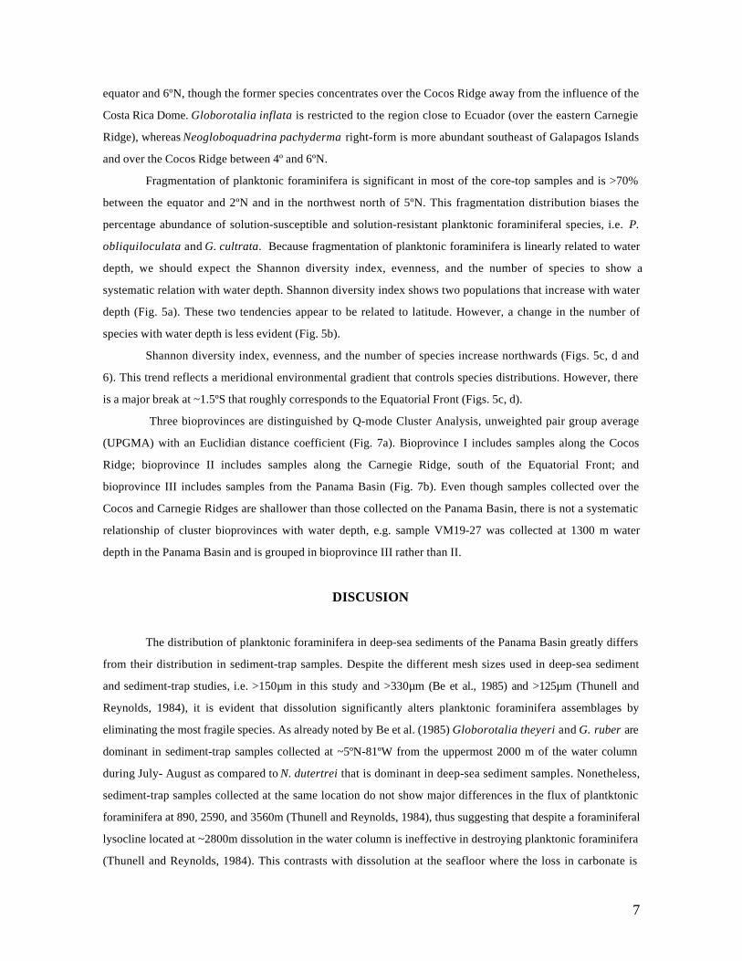
Fragmentation of planktonic foraminifera is significant in most of the core-top samples and is >70%

between the equator and 2ºN and in the northwest north of 5ºN. This fragmentation distribution biases the

percentage abundance of solution-susceptible and solution-resistant planktonic foraminiferal species, i.e. P.

obliquiloculata and G. cultrata. Because fragmentation of planktonic foraminifera is linearly related to water

depth, we should expect the Shannon diversity index, evenness, and the number of species to show a

systematic relation with water depth. Shannon diversity index shows two populations that increase with water

depth (Fig. 5a). These two tendencies appear to be related to latitude. However, a change in the number of

species with water depth is less evident (Fig. 5b).

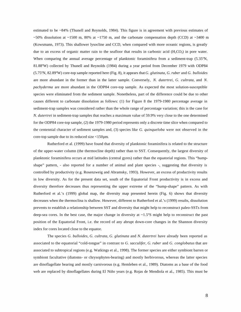
Shannon diversity index, evenness, and the number of species increase northwards (Figs. 5c, d and

6). This trend reflects a meridional environmental gradient that controls species distributions. However, there

is a major break at ~1.5ºS that roughly corresponds to the Equatorial Front (Figs. 5c, d).

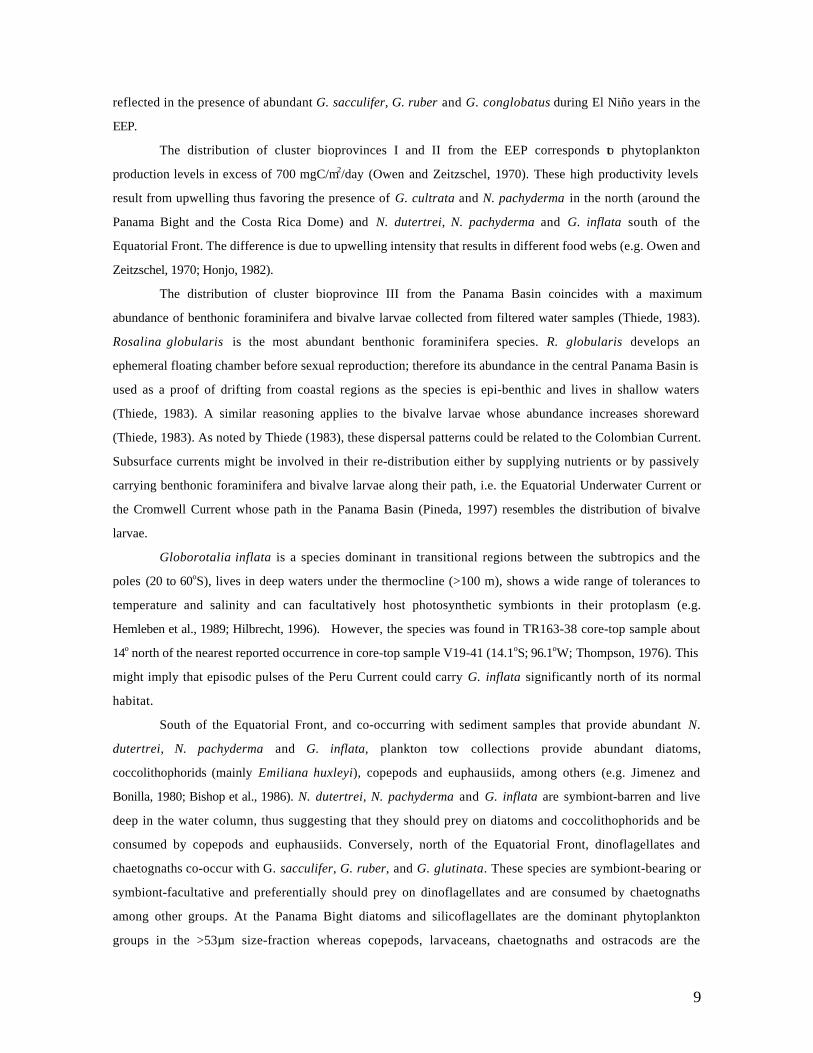
Three bioprovinces are distinguished by Q-mode Cluster Analysis, unweighted pair group average

(UPGMA) with an Euclidian distance coefficient (Fig. 7a). Bioprovince I includes samples along the Cocos

Ridge; bioprovince II includes samples along the Carnegie Ridge, south of the Equatorial Front; and

bioprovince III includes samples from the Panama Basin (Fig. 7b). Even though samples collected over the

Cocos and Carnegie Ridges are shallower than those collected on the Panama Basin, there is not a systematic

relationship of cluster bioprovinces with water depth, e.g. sample VM19-27 was collected at 1300 m water

depth in the Panama Basin and is grouped in bioprovince III rather than II.

DISCUSION

The distribution of planktonic foraminifera in deep-sea sediments of the Panama Basin greatly differs

from their distribution in sediment-trap samples. Despite the different mesh sizes used in deep-sea sediment

and sediment-trap studies, i.e. >150µm in this study and >330µm (Be et al., 1985) and >125µm (Thunell and

Reynolds, 1984), it is evident that dissolution significantly alters planktonic foraminifera assemblages by

eliminating the most fragile species. As already noted by Be et al. (1985) Globorotalia theyeri and G. ruber are

dominant in sediment-trap samples collected at ~5ºN-81ºW from the uppermost 2000 m of the water column

during July- August as compared to N. dutertrei that is dominant in deep-sea sediment samples. Nonetheless,

sediment-trap samples collected at the same location do not show major differences in the flux of plantktonic

foraminifera at 890, 2590, and 3560m (Thunell and Reynolds, 1984), thus suggesting that despite a foraminiferal

lysocline located at ~2800m dissolution in the water column is ineffective in destroying planktonic foraminifera

(Thunell and Reynolds, 1984). This contrasts with dissolution at the seafloor where the loss in carbonate is

8

estimated to be ~84% (Thunell and Reynolds, 1984). This figure is in agreement with previous estimates of

~50% dissolution at ~1500 m, 80% at ~1750 m, and the carbonate compensation depth (CCD) at ~3400 m

(Kowsmann, 1973). This shallower lysocline and CCD, when compared with more oceanic regions, is greatly

due to an excess of organic matter rain to the seafloor that results in carbonic acid (H2CO3) in pore water.

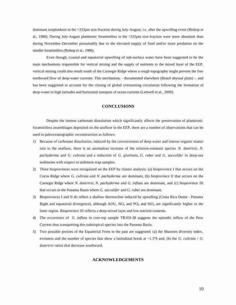
When comparing the annual average percentage of planktonic foraminifera from a sediment-trap (5.35ºN,

81.88ºW) collected by Thunell and Reynolds (1984) during a year period from December 1979 with ODP84

(5.75ºN, 82.89ºW) core-top sample reported here (Fig. 8), it appears that G. glutinata, G. ruber and G. bulloides

are more abundant in the former than in the latter sample. Conversely, N. dutertrei, G. cultrata, and N.

pachyderma are more abundant in the ODP84 core-top sample. As expected the most solution-susceptible

species were eliminated from the sediment sample. Nonetheless, part of the difference could be due to other

causes different to carbonate dissolution as follows: (1) for Figure 8 the 1979-1980 percentage average in

sediment-trap samples was considered rather than the whole range of percentage variation; this is the case for

N. dutertrei in sediment-trap samples that reaches a maximum value of 59.9% very close to the one determined

for the ODP84 core-top sample, (2) the 1979-1980 period represents only a discrete time slice when compared to

the centennial character of sediment samples and, (3) species like G. quinqueloba were not observed in the

core-top sample due to its reduced size <150µm.

Rutherford et al. (1999) have found that diversity of planktonic foraminifera is related to the structure

of the upper-water column (the thermocline depth) rather than to SST. Consequently, the largest diversity of

planktonic foraminifera occurs at mid latitudes (central gyres) rather than the equatorial regions. This “hump-

shape” pattern, - also reported for a number of animal and plant species -, suggesting that diversity is

controlled by productivity (e.g. Rosenzweig and Abramsky, 1993). However, an excess of productivity results

in low diversity. As for the present data set, south of the Equatorial Front productivity is in excess and

diversity therefore decreases thus representing the upper extreme of the “hump-shape” pattern. As with

Rutherford et al.’s (1999) global map, the diversity map presented herein (Fig. 6) shows that diversity

decreases when the thermoclina is shallow. However, different to Rutherford et al.’s (1999) results, dissolution

prevents to establish a relationship between SST and diversity that might help to reconstruct paleo-SSTs from

deep-sea cores. In the best case, the major change in diversity at ~1.5ºS might help to reconstruct the past

position of the Equatorial Front, i.e. the record of any abrupt down-core changes in the Shannon diversity

index for cores located close to the equator.

The species G. bulloides, G. cultrata, G. glutinata and N. dutertrei have already been reported as

associated to the equatorial “cold-tongue” in contrast to G. sacculifer, G. ruber and G. conglobatus that are

associated to subtropical regions (e.g. Watkings et al., 1998). The former species are either symbiont barren or

symbiont facultative (diatoms- or chrysophytes-bearing) and mostly herbivorous, whereas the latter species

are dinoflagellate bearing and mostly carnivorous (e.g. Hemleben et al., 1989). Diatoms as a base of the food

web are replaced by dinoflagellates during El Niño years (e.g. Rojas de Mendiola et al., 1985). This must be

9

reflected in the presence of abundant G. sacculifer, G. ruber and G. conglobatus during El Niño years in the

EEP.

The distribution of cluster bioprovinces I and II from the EEP corresponds to phytoplankton

production levels in excess of 700 mgC/m2/day (Owen and Zeitzschel, 1970). These high productivity levels

result from upwelling thus favoring the presence of G. cultrata and N. pachyderma in the north (around the

Panama Bight and the Costa Rica Dome) and N. dutertrei, N. pachyderma and G. inflata south of the

Equatorial Front. The difference is due to upwelling intensity that results in different food webs (e.g. Owen and

Zeitzschel, 1970; Honjo, 1982).

The distribution of cluster bioprovince III from the Panama Basin coincides with a maximum

abundance of benthonic foraminifera and bivalve larvae collected from filtered water samples (Thiede, 1983).

Rosalina globularis is the most abundant benthonic foraminifera species. R. globularis develops an

ephemeral floating chamber before sexual reproduction; therefore its abundance in the central Panama Basin is

used as a proof of drifting from coastal regions as the species is epi-benthic and lives in shallow waters

(Thiede, 1983). A similar reasoning applies to the bivalve larvae whose abundance increases shoreward

(Thiede, 1983). As noted by Thiede (1983), these dispersal patterns could be related to the Colombian Current.

Subsurface currents might be involved in their re-distribution either by supplying nutrients or by passively

carrying benthonic foraminifera and bivalve larvae along their path, i.e. the Equatorial Underwater Current or

the Cromwell Current whose path in the Panama Basin (Pineda, 1997) resembles the distribution of bivalve

larvae.

Globorotalia inflata is a species dominant in transitional regions between the subtropics and the

poles (20 to 60oS), lives in deep waters under the thermocline (>100 m), shows a wide range of tolerances to

temperature and salinity and can facultatively host photosynthetic symbionts in their protoplasm (e.g.

Hemleben et al., 1989; Hilbrecht, 1996). However, the species was found in TR163-38 core-top sample about

14o north of the nearest reported occurrence in core-top sample V19-41 (14.1oS; 96.1oW; Thompson, 1976). This

might imply that episodic pulses of the Peru Current could carry G. inflata significantly north of its normal

habitat.

South of the Equatorial Front, and co-occurring with sediment samples that provide abundant N.

dutertrei, N. pachyderma and G. inflata, plankton tow collections provide abundant diatoms,

coccolithophorids (mainly Emiliana huxleyi), copepods and euphausiids, among others (e.g. Jimenez and

Bonilla, 1980; Bishop et al., 1986). N. dutertrei, N. pachyderma and G. inflata are symbiont-barren and live

deep in the water column, thus suggesting that they should prey on diatoms and coccolithophorids and be

consumed by copepods and euphausiids. Conversely, north of the Equatorial Front, dinoflagellates and

chaetognaths co-occur with G. sacculifer, G. ruber, and G. glutinata. These species are symbiont-bearing or

symbiont-facultative and preferentially should prey on dinoflagellates and are consumed by chaetognaths

among other groups. At the Panama Bight diatoms and silicoflagellates are the dominant phytoplankton

groups in the >53µm size-fraction whereas copepods, larvaceans, chaetognaths and ostracods are the

10

dominant zooplankton in the >333µm size-fraction during July-August, i.e. after the upwelling event (Bishop et

al., 1986). During July-August planktonic foraminifera in the >333µm size-fraction were more abundant than

during November-December presumably due to the elevated supply of food and/or more predation on the

smaller foraminifera (Bishop et al., 1986).

Even though, coastal and equatorial upwelling of sub-surface water have been suggested to be the

main mechanisms responsible for vertical mixing and the supply of nutrients to the mixed layer of the EEP,

vertical mixing could also result south of the Carnegie Ridge where a rough topography might prevent the free

northward flow of deep-water currents. This mechanism, - documented elsewhere (Brazil abyssal plain) -, and

has been suggested to account for the closing of global overturning circulation following the formation of

deep-water in high latitudes and horizontal transport of ocean currents (Ledwell et al., 2000).

CONCLUSIONS

Despite the intense carbonate dissolution which significantly affects the preservation of planktonic

foraminifera assemblages deposited on the seafloor in the EEP, there are a number of observations that can be

used in paleoceanographic reconstruction as follows:

1) Because of carbonate dissolution, induced by the corrosiveness of deep water and intense organic matter

rain to the seafloor, there is an anomalous increase of the solution-resistant species N. dutertrei, N.

pachyderma and G. cultrata and a reduction of G. glutinata, G. ruber and G. sacculifer in deep-sea

sediments with respect to sediment-trap samples.

2) Three bioprovinces were recognized on the EEP by cluster analysis: (a) bioprovince I that occurs on the

Cocos Ridge where G. cultrata and N. pachyderma are dominant, (b) bioprovince II that occurs on the

Carnegie Ridge where N. dutertrei, N. pachyderma and G. inflata are dominant, and (c) bioprovince III

that occurs in the Panama Basin where G. sacculifer and G. ruber are dominant.

3) Bioprovinces I and II do reflect a shallow thermocline induced by upwelling (Costa Rica Dome - Panama

Bight and equatorial divergence), although AOU, NO3 and PO4 and SiO2 are significantly higher in the

latter region. Bioprovince III reflects a deep-mixed layer and low nutrient contents.

4) The occurrence of G. inflata in core-top sample TR163-38 suggests the episodic inflow of the Peru

Current thus transporting this subtropical species into the Panama Basin.

5) Two possible proxies of the Equatorial Front in the past are suggested: (a) the Shannon diversity index,

evenness and the number of species that show a latitudinal break at ~1.5ºS and, (b) the G. cultrata / G.

dutertrei ratios that decrease southward.

ACKNOWLEDGEMENTS

11

This work is part of the research project: “Late Quaternary paleoceanography of the Panama Basin,

Colombian Pacific: Implications for Global Climate Change” funded by Universidad EAFIT – COLCIENCIAS

(Programa Nacional de Medio Ambiente y Habitat). We thank Dr. John Firth (Ocean Drilling Program) and Dr.

Steven Carey (University of Rhode Island, NSF grant OCE-9102410) for kindly providing the core-top samples

and Julliet Betancur for diligently processing the samples. Maria Isabel Acevedo and Wilton Echavarria are

acknowledged for their logistic support. Christina Ravelo kindly provided foraminifera countings from six core-

top samples (Faul et al., 2000 study). We thank Georges Vernette for a careful review of the manuscript.

12

REFERENCES

Anderson, D. M., Prell, W. L., and N. J. Barrat. 1989. Estimates of sea surface temperature in the Coral Sea at

the last glacial maximum. Paleoceanogr., 4:615-627.

Be, A. W. H., Bishop, J. K. B., Sverdlove, M. S. and W. D. Gardner. 1985. Standing stock, vertical distribution

and flux of planktonic foraminifera in the Panama Basin. Marine Micropaleontology 9, 307-333.

Bishop, J. K. B. and J. Marra. 1984. Variations in primary production and particulate carbon flux through the

base of the euphotic zone at the site of the Sediment Trap Intercomparison Experiment (Panama Basin).

J. Mar. Res., 42:189-206.

Bishop, J. K. B., Stephen, J. C. and P. H. Wiebe. 1986. Particulate matter distributions, chemistry and flux in the

Panama Basin: Response to environmental forcing. Prog. Oceanog. 17:1-59.

Broecker, W. S. and G. H. Denton. 1989. The role of ocean-atmosphere reorganizations in glacial cycles.

Geochim. Cosmochim. Acta, 53:2465-2502.

CLIMAP Project Members, 1976. The surface of the ice-age earth. Science, 191:1131-1137.

Cortes, E. A., Bulla, J. G. and C. Parada. 1990. Foraminíferos planctónicos en sedimentos superficiales del

Pacifico Colombiano. VII Seminario Nacional de las Ciencias y Tecnologías del Mar, Memorias, 210-223.

Darling, K. F., Wade, C. M., Steward, I. A., Kroon, D., Digle, R. and A. J. Leigh. 2000. Molecular evidence for

genetic mixing of Arctic and Antarctic subpolar populations of planktonic foraminifers. Nature, 405:43-

47.

Fairbanks, R. G., Sverdlove, M., Free, R., Wiebe, P. H. and A. W. H. Be. 1982. Vertical distribution and isotopic

fractionation of living planktonic foraminifera from the Panama Basin. Nature, 298:841-844.

Faul, K. L., Ravelo, A. C. and M. L. Delaney. 2000. Reconstructions of upwelling, productivity and photic zone

depth in the eastern equatorial Pacific Ocean using planktonic foraminiferal stable isotopes and

abundances. J. Foram. Res. 30(2):110-125.

Forsbergh, E. D. 1969. On the climatology, oceanography and fisheries of the Panama Bight. - Inter-Amer.

Trop. Tuna Comm. Bull., v. 30, p. 141-170.

Hemleben, G., Spindler, M. and R. O. Anderson. 1989. Modern Planktonic Foraminifera. Springer, New York,

363 p.

Hilbrecht, H. 1996. Extant planktonic foraminifera and the physical environment in the Atlantic and Indian

Oceans – An Atlas based on CLIMAP and Levitus (1982) data. Mitt. Geol. Inst. Eidgen. Tech.

Hochschule and Univ. Zurich N. F. 300, 93 p.

Honjo, S. 1982. Seasonality and interaction of biogenic and lithogenic particulate flux at the Panama Basin.

Science, 218:883-884.

Jimenez, R. and D. Bonilla. 1980. Composicion y distribucion de la biomasa del plancton en el Frente Equatorial.

Acta Oceanográfica del Pacifico INOCAR, 1(1):19-64.

13

Kowsmann, R. O. 1973. Coarse components in surface sediments of the Panama Basin, eastern equatorial

Pacific. J. Geol., 81:473-494.

Ledwell, J. R., Montgomery, E. T., Polzin, K. L., Laurent, L. C. St., Schmitt, R. W. and J. M. Tole. 2000. Evidence

for enhanced mixing over rough topography in the abyssal ocean. Nature, 403:179-182.

Levitus, S., Burgett, R. and P. Boyer. 1994. World Ocean Atlas. NOAA, US Dept. Commerce, Washington D.C.

Homepage: http://ingrid.ldgo.columbia.edu/SOURCES/.LEVITUS94/.

Lonsdale, P. E. and B. T. Malfait. 1974. Abyssal dunes of foraminiferal sand on the Carnegie Ridge. GSA Bull.,

85:1697-1712.

Mix, A. C., Morey, A. E., Pisias, N. G. and S. W. Hostetler. 1999. Foraminiferal faunal estimates of

paleotemperature: Circumventing the no-analog problem yields cool ice age tropics. Paleoceanogr.,

14(3):350-359.

Okuda, T., Suescum, R. T., Valencia, M. and A. Rodriguez. 1983. Variación estacional de la posición del Frente

Ecuatorial y su efecto sobre la fertilidad de las aguas superficiales ecuatorianas. Acta Oceanográfica del

Pacifico INOCAR, 2(1):53-84.

Owen, R. W. and B. Zeitzschel. 1970. Phytoplankton production: seasonal change in the oceanic eastern

tropical Pacific. Mar. Biol., 7:32-36.

Pak, H. and J. R. V. Zaneveld. 1974. Equatorial Front in the eastern Pacific Ocean. J. Phys. Oceanogr., 4:570-578.

Parker, F. L. 1962. Planktonic foraminiferal species in Pacific sediments. Micropaleontology, 8(2):219-254.

Pawlowski, J. 2000. Introduction to the molecular systematics of foraminifera. Micropaleontology, 46(1):1-12.

Pineda, A. R. 1997. La Corriente de Cromwell durante el fenómeno de La Niña de 1996 y el fenómeno de El Niño

de 1997, sobre la Cuenca del Pacifico Colombiano. CCCP Boletín Científico, Armada Nacional

(Colombia), 6:109-122.

Pisias, N. G. and A. C. Mix. 1997. Spatial and temporal oceanographic variability of the eastern equatorial

Pacific during the late Pleistocene: Evidence from radiolarian microfossils. Paleoceanography, 12:381-

393.

Rojas de Mendiola, B., Gomez, O. and B. Ochoa. 1985. Identificación del fenomeno “El Niño” a traves de los

organismos fitoplanctónicos. Bol. Instituto del Mar del Peru:23-31.

Rosenzweig, M. L. and Z. Abramsky. 1993. How are diversity and productivity related? In: R. E. Ricklefs, D.

Schluter (eds.) Species Diversity in Ecological Communities: Historical and Geographical Perspectives.

Univ. Chicago Press, 52-65.

Rutherford S., D’Hont, S. and W. Prell. 1999. Environmental controls on the geographic distribution of

zooplankton diversity. Nature, 400:749-752.

Stevenson, M. 1970. Circulation in the Panama Bight. J. Geoph. Res., 75(3):659-672.

Tchantsev, V. and E. Cabrera. 1998. Algunos aspectos de investigación de la formación del régimen

oceanografico en el Pacifico Colombiano. Boletín Científico CCCP, 7:7-19.

14

Thiede, J. 1983. Skeletal plankton and nekton in upwelling water masses off northwestern South America and

northwest Africa. In: Coastal Upwelling. Its sedimentary record. Art A: Responses of the sedimentary

regime to present coastal upwelling (E. Suess, J. Thiede, eds.), Nato, Plenum Press, 183-207.

Thompson, P. R. 1976. Planktonic foraminiferal dissolution and the progress towards a Pleistocene Equatorial

Pacific transfer function. J. Foram. Res., 6(3):208-227.

Thunell, R. C., Keir, R. S. and S. Honjo. 1981. Calcite dissolution: An in situ study in the Panama Basin.

Science, 212:659-661.

Thunell, R. C., Curry, W. B. and S. Honjo. 1983. Seasonal variation in the flux of planktonic foraminifera: time

series sediment trap results from the Panama Basin. Earth Planet. Sci. Letters, 64:44-55

Thunell, R. C. and L. A. Reynolds. 1984. Sedimentation of planktonic foraminifera: Seasonal changes in species

flux in the Panama Basin. Micropaleont., 30:243-262.

Toggweiler, J. R., Dixon, K. and K. Bryan. 1989. Simulation in a coarse-resolution world ocean model, 1. Steady

state prebomb distributions. J. Geophys. Res., 94, C6:8217-8242.

Tomczak, M. and J. S. Godfrey. 1994. Regional Oceanography: An Introduction. Pergamon, Oxford, 422 pp.

Van Andel, T. H. 1973. Texture and dispersal of sediments in the Panama Basin. J. Geology, 81:434-457.

Watkings, J. M., Mix, A. C. and J. Wilson. 1998. Living planktic foraminifera in the central tropical Pacific

Ocean: articulating the equatorial “cold tongue” during La Niña, 1992. Mar. Micropaleont., 33:157-174.

Wooster, W. S. 1969. Equatorial Front between Peru and Galapagos. Deep-Sea Res., 16:407-419.

Wyrkti, K. 1964. Upwelling in the Costa Rica Dome. Fishery Bull., 63(2):355-372.

Wyrkti, K. 1974. Equatorial currents in the Pacific 1950 to 1970 and their relation to trade winds. J. Phys.

Oceanogr., 4:372-380.

Wyrtki, K. 1981. An estimate of equatorial upwelling in the Pacific. J. Phys. Oceanogr., 11:1205-1214.

Yamashiro, C. 1975. Differential dissolution and transport effects in foraminiferal sediments from the Panama

Basin. Cushman Found. Foram. Res., Spec, Publ., 13:151-159.

For planktonic foraminifera raw data see Microfossil homepage (Data link)

(http://www.geocities.com/CapeCanaveral/Launchpad/4680/).

AUTHORS’S ADDRESS:

Universidad EAFIT, Departamento de Geología, Grupo de Ciencias del Mar, A.A. 3300 Medellín, Colombia. E-

mail jimartin@eafit.edu.co

15

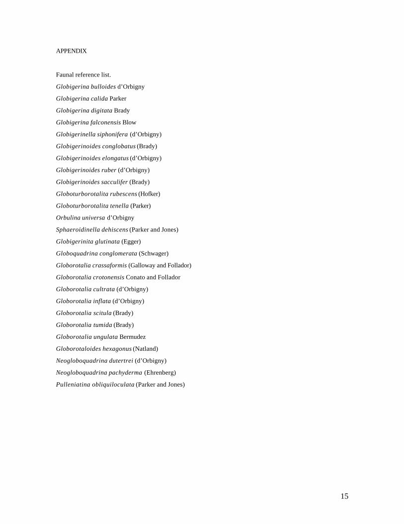
APPENDIX

Faunal reference list.

Globigerina bulloides d’Orbigny

Globigerina calida Parker

Globigerina digitata Brady

Globigerina falconensis Blow

Globigerinella siphonifera (d’Orbigny)

Globigerinoides conglobatus (Brady)

Globigerinoides elongatus (d’Orbigny)

Globigerinoides ruber (d’Orbigny)

Globigerinoides sacculifer (Brady)

Globoturborotalita rubescens (Hofker)

Globoturborotalita tenella (Parker)

Orbulina universa d’Orbigny

Sphaeroidinella dehiscens (Parker and Jones)

Globigerinita glutinata (Egger)

Globoquadrina conglomerata (Schwager)

Globorotalia crassaformis (Galloway and Follador)

Globorotalia crotonensis Conato and Follador

Globorotalia cultrata (d’Orbigny)

Globorotalia inflata (d’Orbigny)

Globorotalia scitula (Brady)

Globorotalia tumida (Brady)

Globorotalia ungulata Bermudez

Globorotaloides hexagonus (Natland)

Neogloboquadrina dutertrei (d’Orbigny)

Neogloboquadrina pachyderma (Ehrenberg)

Pulleniatina obliquiloculata (Parker and Jones)

16

EXPLICACION DE LAS FIGURAS

Figure 1. Physical oceanography of the Eastern Equatorial Pacific Ocean: (a) Sea surface currents (in black), the

Equatorial Undercurrent (in gray), upwelling (in shading) and core-top locations (asterisks), (b) Structure of the

upper-water column along 170ºW; westward currents (in blank) and eastward currents (in hatching). NEC and

SEC = North and South Equatorial Currents, EUC = Equatorial Undercurrent, NECC and SECC = North and

South Equatorial Countercurrents, SSCC = North and South Subsurface Equatorial Countercurrents and, EIC =

Equatorial Intermediate Current. CC = Colombian Current. Note the position of the Equatorial Front. Modified

from Tomczak and Godfrey (1994)

Figure 2. Environmental variables on the Eastern Equatorial Pacific Ocean: (a) sea-surface temperature (SST) in

March, (b) SST in September, (c) mixed-layer depth (m) for March, (d) mixed-layer depth (m) for September, (e)

sea-surface salinity (SSS) for March, (f) SSS for September. Data from Levitus et al. (1994).

Figure 3. Environmental variables on the Eastern Equatorial Pacific Ocean: (a) Apparent oxygen utilization

(AOU), (b) nitrate (NO3) in mmol, (c) dissolved oxygen in ml/l, (d) phosphate (PO4) in mmol, (e) silica (SiO2) in

mmol and, (f) density. Data from Levitus et al. (1994).

Figure 4. Relative abundance (percentage) of planktonic foraminifera in core-top from the Eastern Pacific: (a)

Globigerina bulloides, (b) Globigerinita glutinata, (c) Globigerinoides sacculifer, (d) Globigerinoides

ruber, (e) Globorotalia cultrata, (f) Globorotalia inflata, (g) Neogloboquadrina dutertrei, (h)

Neogloboquadrina pachyderma .

Figure 5. Core-top planktonic foraminiferal diversity for the Eastern Pacific: (a) Shannon diversity index and

evenness against water depth, (b) number of species against water depth, (c) Shannon diversity index and

evenness against latitude, (d) Number of species against latitude.

Figure 6. Shannon diversity index from core-top samples from the Eastern equatorial Pacific Ocean.

Figure 7. Core-top planktonic foraminiferal cluster analyses (UPGMA) for the Eastern Pacific; (a) dendrogram,

(b) bioprovinces map. Core-top locations in asterisks.

Figure 8. Comparison of the percentage abundance of planktonic foraminifera from ODP84 core-top sample (in

shaded; 5.75ºN, 82.89ºW) and a sediment-trap sample (in blank; 5.35ºN, 81.88ºW; Thunell and Reynolds, 1984).

17

18

EXPLICACION DE LAS TABLAS

Table 1. Core-top location for the Eastern Equatorial Pacific Ocean.

Table 2. Percentage abundance of planktonic foraminifera from deep-sea sediments from the Eastern Equatorial

Pacific Ocean. For the full species names see the reference list (Appendix).

19

EXPLICACION DE LA PLANCHA (PLATE 1)

Fig. 1. Globigerina bulloides d’Orbigny, umbilical view.

Fig. 2. Globigerina calida Parker, umbilical view.

Fig. 3. Globigerina calida Parker, dorsal view.

Fig. 4. Globigerinella siphonifera (d’Orbigny).

Fig. 5. Globigerinoides conglobatus (Brady), umbilical view.

Fig. 6. Globigerinoides elongatus (d’Orbigny), umbilical view.

Fig. 7. Globigerinoides ruber (d’Orbigny), umbilical view.

Fig. 8. Globigerinoides ruber (d’Orbigny), dorsal view.

Fig. 9. Globigerinoides sacculifer (Brady), umbilical view.

Fig. 10. Globoturborotalita rubescens (Hofter), umbilical view.

Fig. 11. Globoturborotalita tenella (Parker), umbilical view.

Fig. 12. Orbulina universa d’Orbigny, umbilical view.

Fig. 13. Globoquadrina conglomerata (Schwager), umbilical view.

Fig. 14. Globoquadrina conglomerata (Schwager), dorsal view.

Fig. 15. Globorotaloides hexagonus (Natland), dorsal view.

Fig. 16. Globorotalia cultrata (d’Orbigny), umbilical view.

Fig. 17. Globorotalia cultrata (d’Orbigny), dorsal view.

Fig. 18. Globorotalia inflata (d’Orbigny), umbilical view.

Fig. 19. Globorotalia inflata (d’Orbigny), dorsal view.

Fig. 20. Globorotalia tumida (Brady), umbilical view.

Fig. 21. Globorotalia tumida (Brady), dorsal view.

Fig. 22. Neogloboquadrina dutertrei (d’Orbigny), umbilical view.

Fig. 23. Neogloboquadrina dutertrei (d’Orbigny), dorsal view.

Fig. 24. Pulleniatina obliquiloculata (Parker y Jones), umbilical view.

Fig. 25. Pulleniatina obliquiloculata (Parker y Jones), profile view.

Fig. 26. Neogloboquadrina pachyderma (Ehrenberg), umbilical view.

Fig. 27. Neogloboquadrina pachyderma (Ehrenberg), dorsal view.

Fig. 28. Sphaeroidinella dehiscens (Parker and Jones), dorsal view.

Fig. 29. Globigerinita glutinata (Egger), dorsal view.

Fig. 30. Globigerinita glutinata (Egger), ventral view

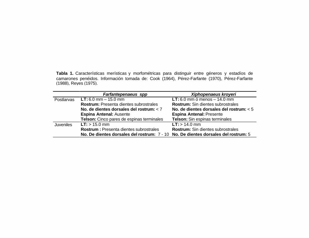
Farfantepenaeus spp Xiphopenaeus kroyeriPostlarvas LT: 6.0 mm – 15.0 mm

Rostrum: Presenta dientes subrostralesNo. de dientes dorsales del rostrum: < 7Espina Antenal: AusenteTelson: Cinco pares de espinas terminales

LT: 6.0 mm ó menos – 14.0 mmRostrum: Sin dientes subrostralesNo. de dientes dorsales del rostrum: < 5Espina Antenal: PresenteTelson: Sin espinas terminales

Juveniles LT: > 15.0 mmRostrum : Presenta dientes subrostralesNo. De dientes dorsales del rostrum: 7 - 10

LT: > 14.0 mmRostrum: Sin dientes subrostralesNo. De dientes dorsales del rostrum: 5

Tabla 1. Características merísticas y morfométricas para distinguir entre géneros y estadíos decamarones penéidos. Información tomada de: Cook (1964), Pérez-Farfante (1970), Pérez-Farfante(1988), Reyes (1975).

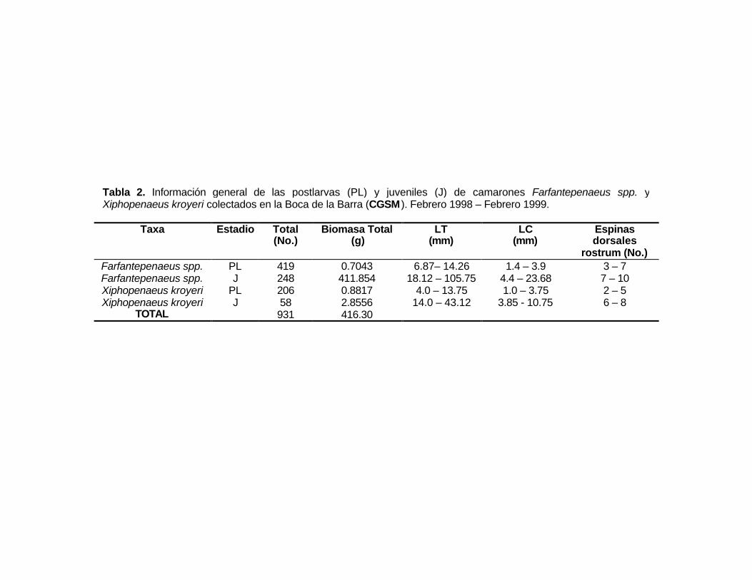
Taxa Estadio Total(No.)

Biomasa Total (g)

LT(mm)

LC(mm)

Espinasdorsales

rostrum (No.)Farfantepenaeus spp. PL 419 0.7043 6.87– 14.26 1.4 – 3.9 3 – 7Farfantepenaeus spp. J 248 411.854 18.12 – 105.75 4.4 – 23.68 7 – 10Xiphopenaeus kroyeri PL 206 0.8817 4.0 – 13.75 1.0 – 3.75 2 – 5Xiphopenaeus kroyeri J 58 2.8556 14.0 – 43.12 3.85 - 10.75 6 – 8

TOTAL 931 416.30

Tabla 2. Información general de las postlarvas (PL) y juveniles (J) de camarones Farfantepenaeus spp. yXiphopenaeus kroyeri colectados en la Boca de la Barra (CGSM ). Febrero 1998 – Febrero 1999.

Taxa Estadio Longitud Total(mm)

LongitudCaparazón

(mm)

EspinasDorsales

Rostrum (No.)

Área de Estudio Autor y Fecha

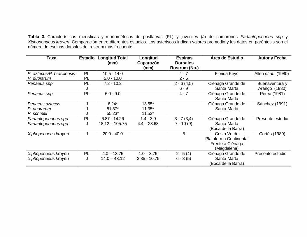
P. aztecus/P. brasiliensisP. duorarum

PLPL

10.5 - 14.05.0 - 10.0

4 - 72 - 6

Florida Keys Allen et al. (1980)

Penaeus spp PLJ

7.2 - 10.2 2 - 6 (4,5)6 - 9

Ciénaga Grande deSanta Marta

Buenaventura yArango (1980)

Penaeus spp. PL 6.0 - 9.0 4 - 7 Ciénaga Grande deSanta Marta

Perea (1981)

Penaeus aztecusP. duorarumP. schmitii

JJJ

6.24*51.37*55.23*

13.55*11.35*11.53*

Ciénaga Grande deSanta Marta

Sánchez (1991)

Farfantepenaeus sppFarfantepenaeus spp

PLJ

6.87 - 14.2618.12 – 105.75

1.4 - 3.94.4 – 23.68

3 - 7 (3,4)7 - 10 (9)

Ciénaga Grande deSanta Marta

(Boca de la Barra)

Presente estudio

Xiphopenaeus kroyeri J 20.0 - 40.0 5 Costa VerdePlataforma Continental

Frente a Ciénaga(Magdalena)

Cortés (1989)

Xiphopenaeus kroyeriXiphopenaeus kroyeri

PLJ

4.0 – 13.7514.0 – 43.12

1.0 – 3.753.85 - 10.75

2 - 5 (4)6 - 8 (5)

Ciénaga Grande deSanta Marta

(Boca de la Barra)

Presente estudio

Tabla 3. Características merísticas y morfométricas de postlarvas (PL) y juveniles (J) de camarones Farfantepenaeus spp yXiphopenaeus kroyeri. Comparación entre diferentes estudios. Los asteriscos indican valores promedio y los datos en paréntesis son elnúmero de espinas dorsales del rostrum más frecuente.

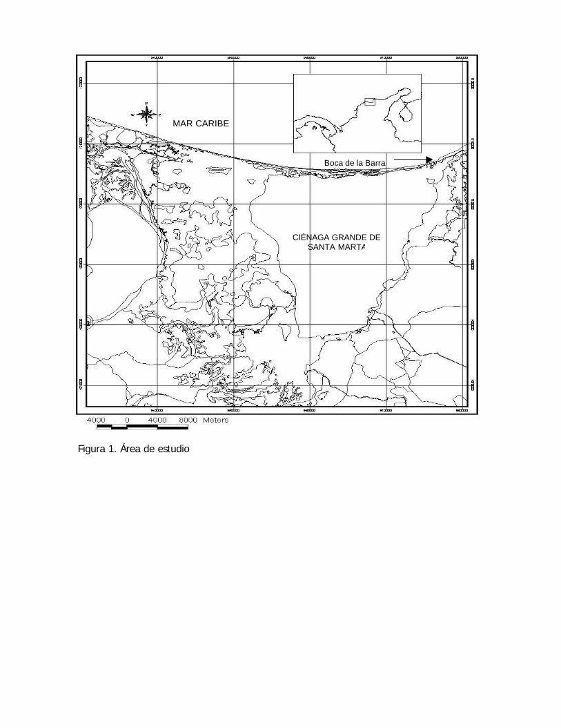
Figura 1. Área de estudio

MAR CARIBE

CIÉNAGA GRANDE DESANTA MARTA

Boca de la Barra

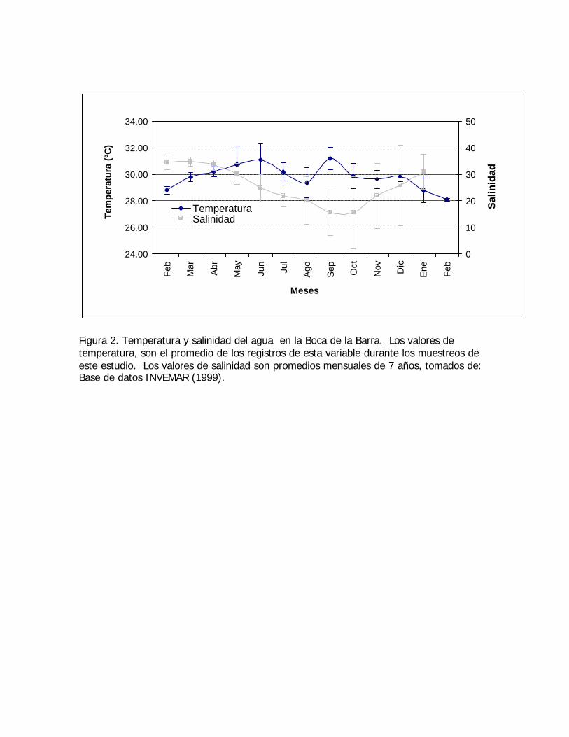
Figura 2. Temperatura y salinidad del agua en la Boca de la Barra. Los valores detemperatura, son el promedio de los registros de esta variable durante los muestreos deeste estudio. Los valores de salinidad son promedios mensuales de 7 años, tomados de:Base de datos INVEMAR (1999).

24.00

26.00

28.00

30.00

32.00

34.00

Feb

Mar

Abr

May

Jun

Jul

Ago

Sep Oct

Nov Dic

Ene Feb

Meses

Tem

per

atu

ra (

ºC)

0

10

20

30

40

50

Sal

inid

ad

TemperaturaSalinidad

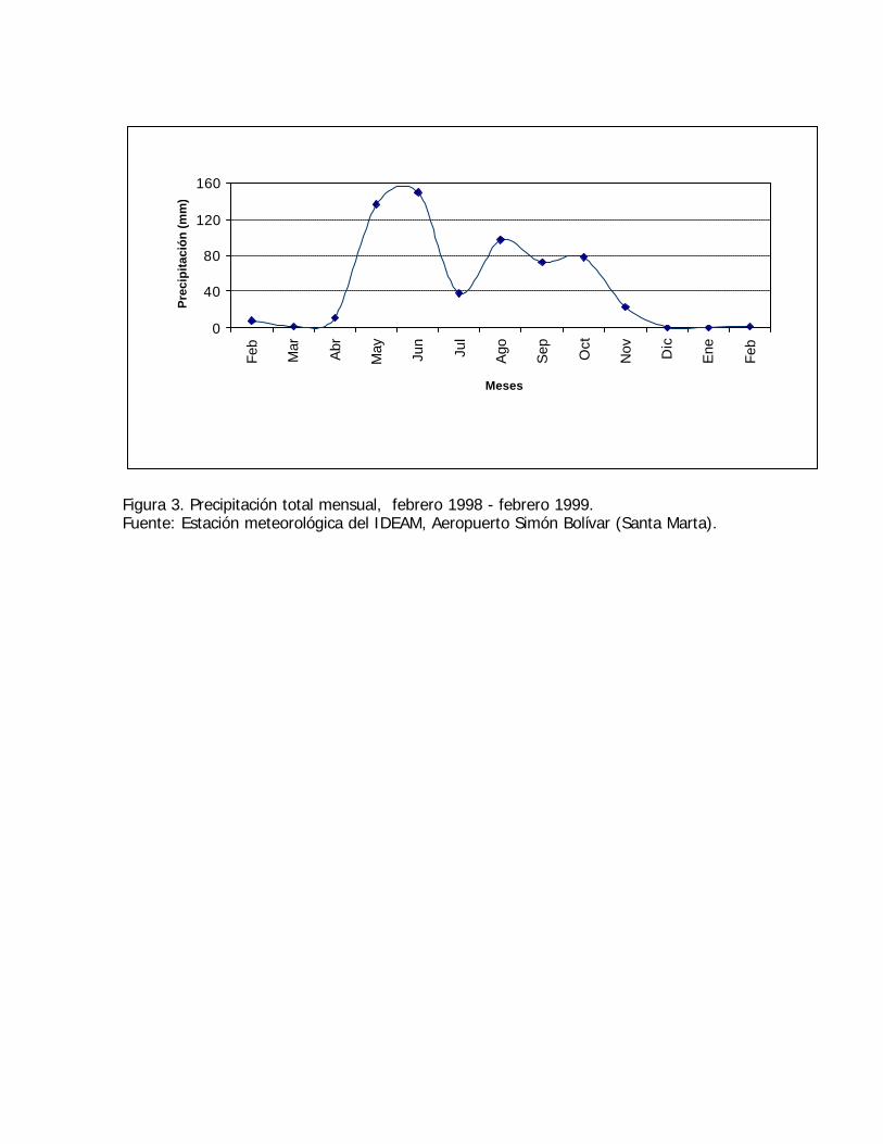
Figura 3. Precipitación total mensual, febrero 1998 - febrero 1999.Fuente: Estación meteorológica del IDEAM, Aeropuerto Simón Bolívar (Santa Marta).

0

40

80

120

160

Feb

Mar

Abr

May Jun

Jul

Ago

Sep Oct

Nov Dic

Ene

Feb

Meses

Pre

cip

itac

ión

(mm

)

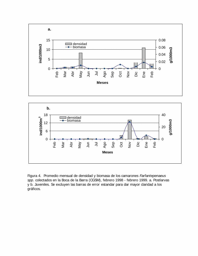
Figura 4. Promedio mensual de densidad y biomasa de los camarones Farfantepenaeusspp. colectados en la Boca de la Barra (CGSM), febrero 1998 - febrero 1999. a. Postlarvasy b. Juveniles. Se excluyen las barras de error estandar para dar mayor claridad a losgráficos.

a.

0

5

10

15

Feb

Mar

Abr

May

Jun

Jul

Ago

Sep Oct

Nov Dic

Ene Feb

Meses

ind/

1000

m3

0

0.02

0.04

0.06

0.08

g/10

00m

3

densidadbiomasa

b.

0

6

12

18

Feb

Mar

Abr

May

Jun

Jul

Ago

Sep Oct

Nov Dic

Ene Fe

bMeses

ind/

1000

m3

0

20

40

g/1

000m

3

densidadbiomasa

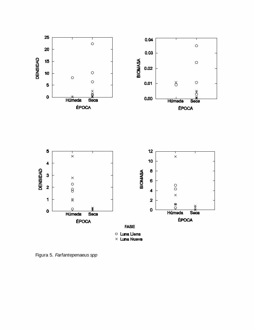
Figura 5. Farfantepenaeus spp

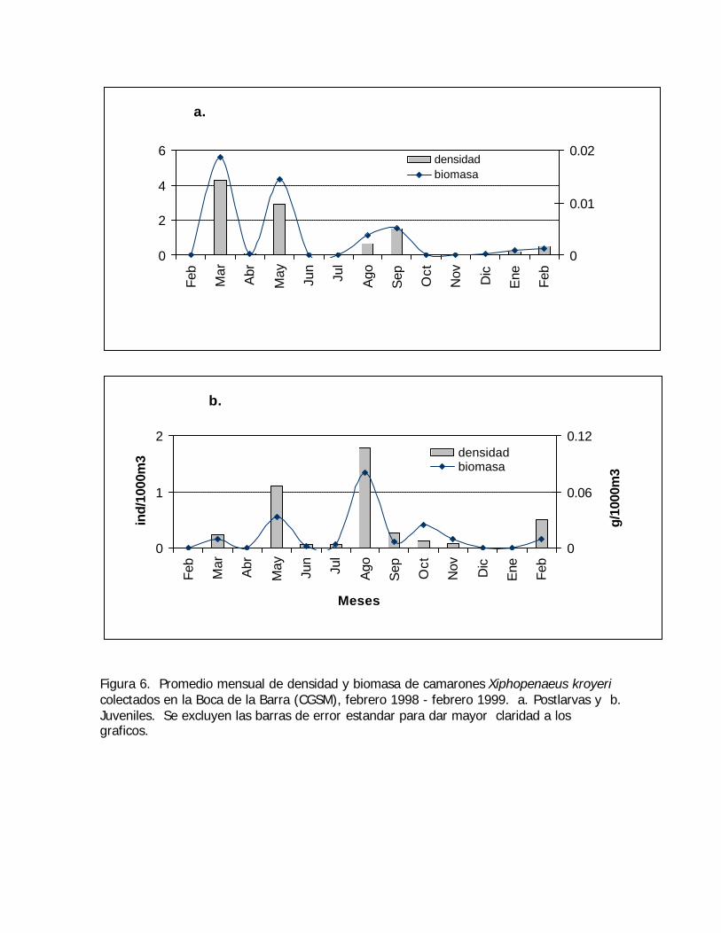
Figura 6. Promedio mensual de densidad y biomasa de camarones Xiphopenaeus kroyericolectados en la Boca de la Barra (CGSM), febrero 1998 - febrero 1999. a. Postlarvas y b.Juveniles. Se excluyen las barras de error estandar para dar mayor claridad a losgraficos.

a.

0

2

4

6

Feb

Mar

Abr

May

Jun

Jul

Ago

Sep Oct

Nov Dic

Ene Feb

0

0.01

0.02densidadbiomasa

b.

0

1

2

Feb

Mar

Abr

May

Jun

Jul

Ago

Sep Oct

Nov Dic

Ene Feb

Meses

ind/

1000

m3

0

0.06

0.12

g/10

00m

3

densidadbiomasa

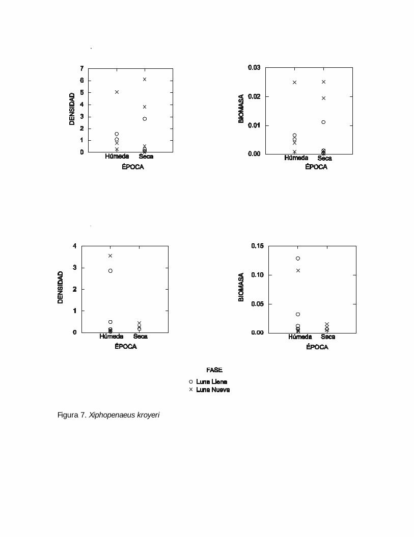
Figura 7. Xiphopenaeus kroyeri

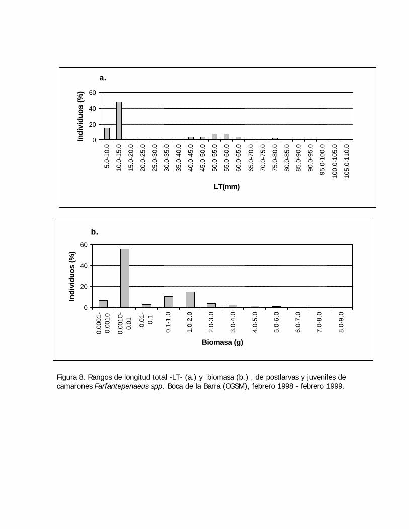
Figura 8. Rangos de longitud total -LT- (a.) y biomasa (b.) , de postlarvas y juveniles decamarones Farfantepenaeus spp. Boca de la Barra (CGSM), febrero 1998 - febrero 1999.

a.

0

20

40

60

5.0-

10.0

10.0

-15.

0

15.0

-20.

0

20.0

-25.

0

25.0

-30.

0

30.0

-35.

0

35.0

-40.

0

40.0

-45.

0

45.0

-50.

0

50.0

-55.

0

55.0

-60.

0

60.0

-65.

0

65.0

-70.

0

70.0

-75.

0

75.0

-80.

0

80.0

-85.

0

85.0

-90.

0

90.0

-95.

0

95.0

-100

.0

100.

0-10

5.0

105.

0-11

0.0

LT(mm)

Indi

vidu

os (%

)

b.

0

20

40

60

0.00

01-

0.00

10

0.00

10-

0.01 0.01

-0.

1

0.1-

1.0

1.0-

2.0

2.0-

3.0

3.0-

4.0

4.0-

5.0

5.0-

6.0

6.0-

7.0

7.0-

8.0

8.0-

9.0

Biomasa (g)

Indi

vidu

os (%

)

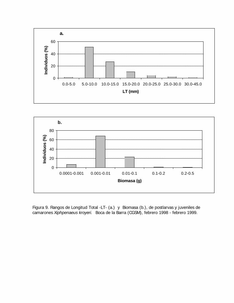
Figura 9. Rangos de Longitud Total -LT- (a.) y Biomasa (b.), de postlarvas y juveniles decamarones Xiphpenaeus kroyeri. Boca de la Barra (CGSM), febrero 1998 - febrero 1999.

a.

0

20

40

60

0.0-5.0 5.0-10.0 10.0-15.0 15.0-20.0 20.0-25.0 25.0-30.0 30.0-45.0

LT (mm)

Indi

vidu

os (%

)

b.

0

20

40

60

80

0.0001-0.001 0.001-0.01 0.01-0.1 0.1-0.2 0.2-0.5

Biomasa (g)

Indi

vidu

os (%

)

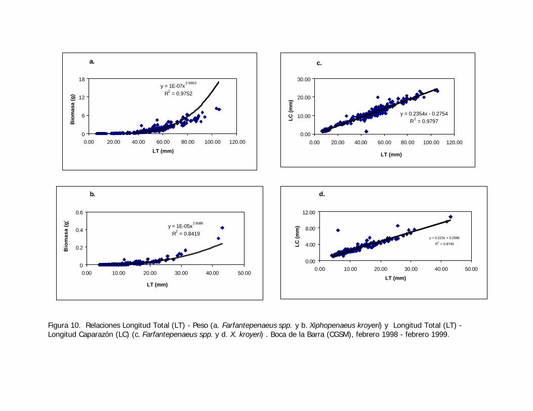
Figura 10. Relaciones Longitud Total (LT) - Peso (a. Farfantepenaeus spp. y b. Xiphopenaeus kroyeri) y Longitud Total (LT) -Longitud Caparazón (LC) (c. Farfantepenaeus spp. y d. X. kroyeri) . Boca de la Barra (CGSM), febrero 1998 - febrero 1999.

a.

y = 1E-07x3.9963

R2 = 0.9752

0

6

12

18

0.00 20.00 40.00 60.00 80.00 100.00 120.00

LT (mm)

Bio

mas

a (g

)

b.

y = 1E-05x2.6586

R2 = 0.8419

0

0.2

0.4

0.6

0.00 10.00 20.00 30.00 40.00 50.00

LT (mm)

Bio

mas

a (g

)c.

y = 0.2354x - 0.2754R2 = 0.9797

0.00

10.00

20.00

30.00

0.00 20.00 40.00 60.00 80.00 100.00 120.00

LT (mm)

LC (m

m)

d.

y = 0.223x + 0.2586

R2 = 0.8745

0.00

4.00

8.00

12.00

0.00 10.00 20.00 30.00 40.00 50.00

LT (mm)

LC (m

m)