Real-Time Forecasts of the Real Price of Oil - frbsf.org · Real-Time Forecasts of the Real Price...

0

Real-Time Forecasts of the Real Price of Oil

July 8, 2011

Christiane Baumeister Lutz Kilian

Bank of Canada University of Michigan

Abstract: We construct a monthly real-time data set consisting of vintages for 1991.1-2010.12 that is suitable for generating forecasts of the real price of oil from a variety of models. We document that revisions of the data typically represent news, and we introduce backcasting and nowcasting techniques to fill gaps in the real-time data. We show that real-time forecasts of the real price of oil can be more accurate than the no-change forecast at horizons up to one year. In some cases real-time MSPE reductions may be as high as 25 percent one month ahead and 24 percent three months ahead. This result is in striking contrast to related results in the literature for asset prices. In particular, recursive vector autoregressive (VAR) forecasts based on global oil market variables tend to have lower MSPE at short horizons than forecasts based on oil futures prices, forecasts based on AR and ARMA models, and the no-change forecast. In addition, these VAR models have consistently higher directional accuracy. We demonstrate how with additional identifying assumptions such VAR models may be used not only to understand historical fluctuations in the real price of oil, but to construct conditional forecasts that reflect hypothetical scenarios about future demand and supply conditions in the market for crude oil. These tools are designed to allow forecasters to interpret their oil price forecast in light of economic models and to evaluate its sensitivity to alternative assumptions. JEL Code: Q43, C53, E32 Key Words: Oil price; real time; forecast; scenario analysis. Acknowledgements: The views in this paper are solely the responsibility of the authors and should not be interpreted as reflecting the views of the Bank of Canada. We thank Ron Alquist for helpful comments. William Wu provided excellent research assistance. Correspondence to: Lutz Kilian, Department of Economics, 611 Tappan Street, Ann Arbor, MI 48109-1220, USA. Email: [email protected].

1

1. Introduction

Although the real price of oil is one of the key variables in the model-based macroeconomic

projections generated by central banks, private sector forecasters, and international

organizations, there have been no studies to date of how best to forecast the real price of oil in

real time. One likely reason is that – unlike for U.S. domestic macroeconomic aggregates – there

is no real-time data set for variables relevant to forecasting the real price of oil.1 In this paper we

remedy this situation by constructing from the original data sources a comprehensive monthly

real-time data set consisting of vintages for 1991.1 through 2010.12, each covering data

extending back to 1973.1. This data set allows the construction of real-time forecasts of the real

price of oil from a variety of models. Both backcasting and nowcasting techniques are used to fill

gaps in the real-time data. In section 2, we show that revisions of most oil market data represent

“news” as defined in De Jong (1987) and Faust, Rogers, and Wright (2005). In other words, there

is little scope for improving forecasts by modeling the revision process. This fact facilitates the

construction of nowcasts to fill in gaps in the availability of real-time data for most series.

In section 3, we use this data set to provide evidence that real oil price forecasts can be

more accurate than the no-change forecast at horizons up to one year. We present results both for

the U.S. refiners’ acquisition cost for crude oil imports, which may be viewed as a proxy for the

price of oil in global markets, and for the WTI spot price which receives most attention in the

media.2 The evaluation window is 1992.1-2010.6. Our evaluation criteria are both the MSPE of

the forecasts and their directional accuracy. We consider a variety of forecasting methods

including versions of methods that have been shown to work well in the related context of

forecasting the nominal price of oil (see, e.g., Alquist, Kilian and Vigfusson 2011). We find that

many forecasting methods perform well compared with the no-change forecast at horizons up to

one year. With some forecasting methods, real-time MSPE reductions may be as high as 25

percent one month ahead and 24 percent three months ahead. This result is in striking contrast to

related results in the literature for real exchange rates or real stock returns. In particular, we show

that recursive vector autoregressive (VAR) forecasts based on global oil market variables tend to

have lower MSPEs at short horizons than forecasts based on oil futures prices, forecasts based on

1 Neither the real-time data set repository maintained by the Federal Reserve Bank of Philadelphia nor the ALFRED data base maintained by the Federal Reserve Bank of St. Louis include such data. Nor does the U.S. Energy Information Administration provide any real-time data sets. 2 We do not consider the Brent price given the limited time span for which that price has existed.

2

AR and ARMA models, and the no-change forecast. In addition, these VAR models have

consistently and often significantly higher directional accuracy with success ratios as high as

65% in real time in some cases. Such success ratios are high by the standards of the empirical

finance literature (see, e.g., Pesaran and Timmermann 1995).

Section 3 also contrasts the real-time forecasting results with results for the same

forecasting models based on ex-post revised data. It is not obvious ex ante whether models

based on ex-post revised data should forecast more accurately than models based on real-time

data. For example, Faust, Rogers and Wright (2003) suggest that real-time forecasts may be

more accurate if agents’ behavior reflects real-time expectations. We find that there are no

further gains in forecast accuracy from using ex-post revised data when using the WTI price, but

substantially larger gains when using the refiners’ acquisition cost for imported oil. In the latter

case, some VAR models produce MSPE gains as high as 33 percent at the one-month horizon, 22

percent at the three-month horizon, and 3% at the six-month horizon. This raises the question of

which aspect of the data collection statistical agencies should focus on to improve the overall

forecast accuracy for the real refiners’ acquisition cost. We find that improving the timely

availability of accurate data on the nominal price of oil has by far the highest payoff. For the

U.S. refiners’ acquisition cost for imports, replacing the nominal price by ex-post revised data

alone suffices to generate forecasts almost as accurate as if all data were ex-post revised and

available in real time. None of the other variables has such a large impact. This conclusion is

further corroborated by the fact that for the WTI price, which is not subject to data revisions and

available without delay, the difference between the VAR forecast accuracy with real-time data

and with ex-post revised data is negligible.

In section 4, we contrast the real-time forecast accuracy of regression-based models with

that of alternative forecasting methods based on oil futures prices or non-oil industrial

commodity prices. We show that models based on oil futures prices do not produce significant

MSPE reductions and have lower directional accuracy than suitably chosen VAR models. We

also make the case that VAR models have advantages over models based on industrial

commodity prices alone.

An important limitation of standard reduced-form forecasting models from a policy point

of view is that they provide no insight into what is driving the forecast and do not allow the

policymaker to explore alternative hypothetical forecast scenarios. Policymakers not only expect

3

oil price forecasts to be interpretable in light of an economic model, but like to evaluate the risks

associated with a baseline forecast based on an extensive analysis of how these forecasts change

with changes in the underlying assumptions. In section 5, we illustrate how with additional

identifying assumptions the VAR forecasting models that we already considered in section 3

may also be used to understand historical fluctuations in the real price of oil and to construct

real-time conditional projections of how the oil price forecast would deviate from the

unconditional forecast benchmark under hypothetical scenarios about future demand and supply

conditions in the global market for crude oil. Examples of such scenarios include an unexpected

surge in speculative demand triggered by civil unrest in an oil-producing country such as Libya,

for example, or an unexpected resurgence of the global business cycle. These tools are designed

to allow end-users to interpret oil price forecasts in light of economic models and to evaluate

their sensitivity to alternative assumptions. The concluding remarks are in section 6.

2. The Real-Time Data Set

Unlike Carlton (2010) and Ravazzolo and Rothman (2010) our focus is not on real-time

forecasting of U.S. real GDP growth on the basis of lagged oil prices, but rather on generating

real-time forecasts of the real price of oil. Our analysis is more closely related to the recent

literature on real-time forecasts of the nominal price of oil (see, e.g., Alquist and Kilian 2010;

Alquist, Kilian, and Vigfusson 2011). Although the real price of oil is one of the key variables in

the model-based macroeconomic projections generated by central banks, private sector

forecasters, and international organizations, there have been no studies to date of how best to

forecast the real price of oil in real time. One reason is that there is no readily available real-time

data set for the variables required in forecasting the real price of oil.

Our first contribution in this paper is the construction of such a data set from a variety of

sources, many of which are not available in electronic form. Our data set is monthly and includes

some raw data that are available in real time and not subject to data revisions such as 1) the WTI

spot price of crude oil, 2) NYMEX oil futures prices at various maturities, 3) an index of the spot

price of industrial raw materials, and 4) an index of bulk dry cargo ocean shipping freight rates

(such as the Baltic Dry Cargo Index). Our data set also includes many time series that are not

available in real time. The latter time series include: 1) the nominal U.S. refiners’ acquisition

cost for crude oil imports, 2) world crude oil production, 3) U.S. crude oil inventories, 4) U.S.

4

petroleum inventories, 5) OECD petroleum inventories. Finally, we collected data for the U.S.

consumer price index for all urban consumers and the U.S. producer price index for crude oil.

The use of real-time data in forecasting raises two distinct complications. First, even

preliminary data may become available only with a lag. Second, past data are continuously

revised. Little is known about the nature of the revisions of oil market data or how these

revisions and delays in data availability affect out-of-sample forecast accuracy.

2.1. Data Sources

Monthly averages of the daily WTI spot price were obtained from the website of the U.S. Energy

Information Administration (EIA). The corresponding average NYMEX oil futures prices are

from Bloomberg. The spot price index of industrial raw materials is from the Commodity

Research Bureau. All other oil market data were obtained from the Monthly Energy Review

published by the EIA. Prior to 1996.1 this publication is not available in electronic form. The

construction of the real-time data set from the historical issues of the Monthly Energy Review is

described in detail below. The nominal shipping rate data are obtained from Kilian (2009) for

1973.1 through 1984.12 and are extrapolated through 2010.12 using the Baltic Dry Cargo Index

(BDI) from Bloomberg. Real-time data for the monthly U.S. consumer price index are obtained

from the Economic Indicators published by the Council of Economic Advisers. These data are

made available by the FRASER data base of the Federal Reserve Bank of St. Louis. Additional

real-time CPI data were obtained from the macroeconomic real-time data base of the Federal

Reserve Bank of Philadelphia. The U.S. producer price index for crude oil is not required in real

time for our analysis and is obtained from the Bureau of Labor Statistics.

2.2. Real-Time Data Revisions

Each issue of the Monthly Energy Review contains the current vintage of oil market data and

differs from the preceding issue in that the historical data may have been partially revised and

that a new monthly observation has been added. Due to space limitations, historical data past a

certain number of months are no longer included in the current report (nor are these historical

data available in electronic form). In constructing the real-time data set we assume that no further

revisions occur to these historical data.

5

Ex-post revised data are constructed from the most up-to-date data downloaded from the

EIA website. The most recent data set available at the time our study was written was for

2010.12. Because the most recent data are still preliminary, we discarded the last six months of

data. The remaining data for 1973.1-2010.6 are treated as ex-post revised data when evaluating

the forecasting accuracy of the candidate models. Although some of the data close to the end of

this sample will not be completely revised after six months, the remaining revisions are likely to

be small enough to be ignored in the interest of a larger evaluation sample that includes the

recent period of oil price volatility.

The difference between the initial release for a given date and the ex-post revised

observation for that date can be decomposed further. We distinguish between in-report revisions

and post-report revisions of each time series. In-report revisions are defined as the log-difference

between the value shown in the most recent vintage available for that date in subsequent issues

of the Monthly Energy Review and the value reported on the first release date. Post-report

revisions refer to the log-difference between the ex-post revised value and the corresponding

value in the most recent vintage available in subsequent issues of the Monthly Energy Review.

Exhibit 1 provides selected descriptive statistics concerning the nature of the data

revisions for each time series. The average number of revisions ranges from 1 for the U.S.

refiners’ acquisition cost for crude oil imports to 9 in the global crude oil production data. Most

revisions occur one month after the first release, but revisions may continue for several years in

some cases. For U.S. oil market data revisions are complete within two years. The relative

frequency of revisions declines over time, but not necessarily monotonically.

For all oil market series, we find that the post-report revisions are essentially zero,

lending credence to our assumption that historical data are not revised further once they are no

longer reported in the Monthly Energy Review. Moreover, the in-report revisions are near zero on

average with very small standard deviations (smaller than 0.1% in all cases), indicating that real-

time forecasts could not be improved by adjusting forecasts by a constant representing the

revision bias. This does not mean that the preliminary data releases are necessarily efficient

forecasts of the final releases, but, as will be shown in section 3.3, for most series the quality of

the preliminary data makes little difference in forecasting the real price of oil.

6

2.3. Backcasting

Our objective is to construct a real-time data set consisting of vintages for 1991.1 through

2010.12, each covering data extending back to 1973.1. The starting date of 1991.1 for the first

vintage was chosen because the Monthly Energy Review was not issued between October and

December of 1990, creating a gap in the real-time data.

One complication in creating the real-time data set is that each vintage as reported by the

EIA only includes data for at most three years. For example, the 1991.1 issue includes data as far

back as 1988.1. This means that the pre-1988.1 data for all vintages have to be approximated by

the ex-post revised data. Given that the post-report revisions, as shown in section 2.2, are zero or

negligible even for more recent data, this backcasting approach is likely to be a good

approximation.

In addition, as we move from one Monthly Energy Review to the next, some of the earlier

observations are no longer reported. There are two alternative approaches to filling in these

missing data. One approach is to rely on ex-post revised data. The other approach postulates that,

once observations are no longer reported, no further data revisions occur, so we can use the most

recent data from earlier vintages to fill in the gaps in the current vintage. Preliminary forecast

evaluations indicated that neither approach results in systematically more accurate out-of-sample

forecasts than the other and that the differences in results are negligible. Throughout this paper

we employ the second approach.

In constructing the monthly U.S. refiners’ acquisition cost for crude oil imports a further

complication arises because these data are only available starting in 1974.1. We followed the

procedure outlined in Mork (1989, p. 741) for extrapolating the refiners’ acquisition cost

backwards to 1973.1. This procedure involves scaling the monthly percent rate of change in the

U.S. crude oil producer price index for 1973.1-1974.1 by the ratio of the growth rate in the

annual refiners’ acquisition cost over the growth rate in the annual U.S. producer price index for

crude oil.

Consistent series for OECD petroleum stocks are not available prior to 1987.12. We

therefore extrapolate the percent change in OECD inventories backwards at the rate of growth of

U.S. petroleum inventories, following Kilian and Murphy (2010). For the post-1987.12 period,

U.S. and OECD petroleum inventory growth rates are highly correlated. We also adjust the real-

time OECD petroleum inventory data to account for changes in the set of OECD members

7

reporting inventories in December 2001. This adjustment is necessary to preserve the

consistency of the real-time and the ex-post revised inventory data. The procedure is to add ex-

post revised data from the EIA on the petroleum inventories of these countries in constructing

real-time equivalents of the OECD petroleum inventory data prior to the change in classification.

Likewise, we adjust the real-time OECD petroleum inventory data contained in the pre-June

1993 issues of the Monthly Energy Review to reflect the addition of East Germany.

Finally, in constructing real-time CPI data we face the problem that the CEA only reports

real-time CPI data for the 12 most recent months of each vintage. We fill in the missing data

back to 1973.1 based on quarterly vintages of monthly real-time CPI data from the Federal

Reserve Bank of Philadelphia, exploiting the fact that observations shown in each vintage

represent the data that were available in the middle of the quarter.

2.4. Data Transformations

The real price of oil is constructed by deflating the nominal price of oil by the U.S. consumer

price index. World oil production is expressed in growth rates. Following Kilian and Murphy

(2010), a proxy for the change in world crude oil inventories is constructed by scaling U.S. crude

oil inventories by the ratio of OECD over U.S. petroleum inventories. This approximation is

required because there are no monthly crude oil inventory data for other countries. Finally, as is

standard in the literature, the measure of global real activity is constructed by cumulating the

growth rate of the index of nominal shipping rates, the resulting nominal index is deflated by the

U.S. consumer price index, and a linear deterministic trend representing increasing returns to

scale in ocean shipping is removed from the real index (see, e.g., Kilian 2009). The resulting

index is designed to capture business cycle fluctuations in global industrial commodity markets.

In constructing the real-time version of this index of global real activity, the linear deterministic

trend is recursively re-estimated in real time.

An interesting question is whether data revisions in these transformed real-time series

represent news or whether they could have been predicted based on the initial data release. We

focus on world oil production growth, the change in global crude oil inventories, and the real

refiners’ acquisition cost for crude oil imports.3 Let ,f pt t tR X X where p

tX denotes the

3 The corresponding revisions in the real WTI price are effectively negligible, making further analysis of that series moot. We also excluded the global real activity index from the analysis. Because the underlying shipping rates are

8

preliminary data release for a given time series and ftX the final release. Under the news

characterization, the statistical agency optimally uses all available information, so revisions of

preliminary data must reflect news that arrives after the preliminary data release. This hypothesis

implies that revisions must be mean zero because otherwise revisions would be predictable. It

can be shown that there is no statistically significant bias in the revisions for any of the three

transformed real-time variables.

As noted by Faust et al. (2005), bias is the simplest form of predictability in revision.

Even in the absence of bias, however, revisions may be predictable based on preliminary data

releases. A more general specification of the news hypothesis implies that 0 in

pt t tR X u

where tu may be serially correlated. Inference is based on HAC standard errors. We find that

only for revisions to world crude oil production the news hypothesis can be rejected at

conventional significance levels. Even in that case, the 2R of the regression is only 3%, however,

suggesting that our ability to predict the revisions will be very limited. Additional evidence in

section 3.3 will confirm this conjecture.

2.5. Nowcasting

A further complication arises because some of the data used in constructing the real price of oil

and its predictors are only available with a delay. Exhibit 1 indicates for each series the number

of missing real-time observations. In some cases, the real-time data become available with a lag

as long as six months. These gaps in the real-time data have to be filled using nowcasting. We

extrapolate the world oil production data based on the average rate of change in world oil

production up to that point in time. The same approach is used for the U.S. consumer price

index. This amounts to treating the price level as a random walk with drift. The U.S. refiners’

acquisition cost for crude oil imports is extrapolated at the rate of growth of the WTI price. Not

surprisingly, this approach dramatically improves out-of-sample forecast accuracy compared

spot prices not subject to revisions and because the effect of the revisions in the CPI on the index is negligible, the only real-time uncertainty in measuring global real activity arises from the trend estimate. Given that trend estimation uncertainty is not related to the data revision process, we abstract from the real activity index in studying the news hypothesis. The analysis in section 3.3 indicates that this trend estimation uncertainty has little effect on out-of-sample forecast accuracy.

9

with using the no-change nowcast because it incorporates unforecastable movements in oil

prices. In nowcasting the global crude oil inventory data, we treat the ratio of OECD over U.S.

petroleum inventories as a random walk and extrapolate U.S. crude oil inventories at their

average rate of change in the past. These nowcasting methods are designed to be simple to

implement, yet accurate. In section 3.3 we provide evidence that more sophisticated nowcasting

rules would not improve forecasting accuracy materially.

3. Real-time Forecast Accuracy

Our objective throughout this paper is to forecast the level of the real price of oil rather than the

log price because it is the real price that matters to policymakers.4 Regression models are

specified in logs, where appropriate, and the forecasts are exponentiated. The forecast horizon is

one, three, six, nine and twelve months.

3.1. Regression-Based Forecasts

Table 1 summarizes the real-time forecast accuracy of ARMA and AR models of the real U.S.

refiners’ acquisition cost for crude oil imports and of the four-variable VAR oil market model of

Kilian and Murphy (2010). The VAR model includes the percent change in global crude oil

production, the Kilian (2009) measure of global real activity (in deviations from trend), the

change in global crude oil inventories and the real U.S. refiners’ acquisition cost for crude oil

imports, as a measure of the real price of crude oil in global oil markets. Table 2 shows the

results for the corresponding models based on the real WTI price. We consider fixed

autoregressive lag orders of 12 and 24. Such lag orders are common in the literature on oil

market VAR models.5 The autoregressive models are estimated alternatively by unrestricted least

squares and by Bayesian shrinkage methods. The forecast accuracy of the latter methods

depends on the choice of the prior for the model parameters. Rather than reporting results for

alternative priors, as is common in related work, we rely on the data-based method of Giannone,

Lenza, and Primiceri (2010) for selecting the prior in real time. This approach avoids the

temptation of searching ex post for priors that generate more accurate forecasts and preserves the

4 In this sense our analysis differs from related work such as Alquist, Kilian and Vigfusson (2011), for example. 5 As shown in Alquist, Kilian and Vigfusson (2011), the forecast accuracy of AR models for the price of oil is not very sensitive to the lag order and similar results would be obtained if the lag order were selected by information criteria. Nor would differencing the real price of oil improve the forecast accuracy of the AR and ARMA models.

10

real-time nature of the forecasting exercise. The ARMA(1,1) model is estimated numerically by

Gaussian maximum likelihood methods.

Table 1a shows that all methods under consideration produce lower recursive MSPEs

than the no-change forecast at least at short horizons. For example, the ARMA(1,1) model

consistently reduces the MSPE by between 8% and 10% at all horizons. Similar results are

obtained with the BAR(24) model. The AR(24) model is somewhat less accurate, indicating

overfitting problems with the least-squares estimate. AR and BAR models with 12 lags also are

somewhat less accurate, indicating the importance of including a larger number of lags.

Even larger short-run MSPE reductions are possible when using the VAR model. For

example, the unrestricted VAR(12) model lowers the one-month recursive MSPE by 25%

compared with the no-change forecast and the three-month recursive MSPE by 19%. At horizon

9 the two models are essentially tied, but at horizon 12, the MSPE reduction is still 3%. The

VAR(12) model in fact is more accurate than the corresponding BVAR(12) model. Not

surprisingly, however, the forecast accuracy of the VAR(24) model is greatly improved by the

use of Bayesian shrinkage estimation methods. Although the BVAR(24) model is not as accurate

as the VAR(12) model by the MSPE metric, it is still much more accurate in the short run than

AR or ARMA models and – unlike any other model – it offers high and often statistically

significant directional accuracy at all horizons. For example, the probability of correctly

predicting the direction of change is 61% at horizon 1 and 65% at horizon 3. Even at horizon 12

it remains as high as 58%. Based on directional accuracy alone, the BVAR(24) model would be

the obvious choice among the models under consideration.

Table 2a shows that for the real WTI price as well most methods under consideration

produce lower recursive MSPEs than the no-change forecast at least at short horizons. The

magnitude of the forecast accuracy gains is typically somewhat smaller. For example, the

ARMA(1,1) model consistently reduces the MSPE by between 6% and 8% at all horizons. Even

more accurate is the BAR(24) model with MSPE reductions between 8% and 10% at all

horizons. Marginally larger short-run MSPE reductions are possible when using the VAR(12)

and BVAR(12) model. These models also have higher directional accuracy than AR and ARMA

models. Finally, although the unrestricted VAR(24) is strictly dominated by the no-change

forecast, the BVAR(24) model dominates the no-change forecast at all horizons with MSPE

reductions as large as 14% at horizon 1, 13% at horizon 3, 6% at horizon 6, and 5% at horizons 9

11

and 12. As in Table 1b, the BVAR(24) model also has the highest directional accuracy among

all models considered with success ratios ranging from 56% at horizon 1 to 61% at horizon 12.

We conclude that notwithstanding some differences between the results in Tables 1 and

2, there is strong evidence that forecasters can beat the random walk benchmark in real time.

Moreover, in both cases the BVAR(24) model offers the best overall combination of low MSPE

and directional accuracy. This forecasting success is perhaps unexpected given the common view

that the price of oil should be viewed as an asset price and like all asset prices is inherently

unpredictable. Our findings are fully consistent, however, with recent work showing that the

price of oil most of the time contains only a small asset price component (see Kilian and Murphy

2010; Kilian and Vega 2011). It is also consistent with evidence that the nominal WTI price of

oil is predictable based on economic fundamentals at short horizons (see Alquist, Kilian, and

Vigfusson 2011).

Although we report tests of statistical significance for the success ratios in Table 1b and

2b, we do not provide measures of statistical significance for the MSPE reductions in Tables 1a

and 2a. The reason is that such tests are not available. The problem is that the underlying time

series are not stationary because they include data that have been revised to different degrees

(see, e.g., Koenig, Dolmas and Piger 2003; Clements and Galvão 2010; Croushore 2011). This

feature of the regression analysis violates the premise of standard asymptotic tests of equal

predictive accuracy. Clark and McCracken (2009) recently proposed an alternative test of equal

predictive accuracy for real-time data, the construction of which requires further assumptions on

the nature of the data revisions and evidence that these assumptions are met in the real-time data.

That test is not designed for iterated forecasts, however, and could not be applied in our context

even if our real-time data satisfied the assumptions of Clark and McCracken (2009). Nor is it

possible to rely on standard bootstrap methods to simulate the critical values of tests of equal

predictive accuracy in our iterated real-time setting. In section 3.2, we will show, however, that

the same regression models generate highly statistically significant rejections of the null of equal

predictive accuracy when applied to ex-post revised data. Moreover, we will show in section 5

that some alternative forecasting methods built on data that are available in real time (and hence

amenable to statistical testing) fail to generate statistically significant reductions in the MSPE

both using ex-post revised and real-time data.

12

3.2. Forecast Accuracy Based on Ex-Post Revised Data

There are four distinct reasons for investigating the forecast accuracy using ex-post revised data.

First, it provides a benchmark against which we can assess how practically important the

distinction between real-time forecasts and conventional forecasts is. Second, this comparison

allows us to determine which aspects of the data collection, if improved, are likely to increase

real-time forecast accuracy the most, as illustrated in section 3.3. Such information is particularly

useful for data providers such the U.S. Energy Information Administration. Third, given the

impossibility of assessing the statistical significance of the real-time MSPE reductions from

iterated AR, ARMA and VAR forecasts, the use of ex-post revised data allows us to provide at

least some sense of how statistically significant these reductions are likely to be. Fourth, the

performance of VAR models on ex-post revised data is of independent interest when

constructing conditional forecasts or forecast scenarios, as shown in section 5. The latter

scenarios must be based on our best estimate of the population dynamics rather than preliminary

estimates from real-time data.

The results in Tables 3 and 4 are the counterparts of the real-time analysis in Tables 1 and

2. The only difference is that all real-time data have been replaced by ex-post revised data. We

treat the data up to 2010.6 in the 2010.12 vintage as our proxy for the ex-post revised data. The

implicit premise is that virtually all data revisions have taken place within half a year. This

premise is largely consistent with the evidence we presented in section 2.

Table 3 for the real U.S. refiners’ acquisition cost shows that using ex-post revised data

there is overwhelming evidence against the random walk forecast model. The MSPE reductions

are both statistically significant based on bootstrap critical values and economically significant.

This conclusion is by no means self-evident because both the no-change forecasts and the

regression-based forecasts tend to benefit from the availability of ex-post revised data. Hence,

the recursive MSPE ratio ex ante could rise or fall.

Table 3 shows, for example, that ARMA models produce statistically significant

reductions in the MSPE at all horizons. The reductions range from 22% to 8%, depending on the

horizon and are much larger in the short run than for real-time data. Very similar results hold for

the BAR(24) model. Even more accurate in the short run is the VAR(12) model which generates

statistically significant reductions of 33% at horizon 1, 22% at horizon 2 and 6% at horizon 3.

The BVAR(24) model by comparison has somewhat lower MSPE, but higher directional

13

accuracy. Even that model still produces highly statistically significant MSPE reductions relative

to the no-change forecast of 27% at horizon 1, 15% at horizon 3, and 3% at horizon 6.

For the real WTI price in Table 4, in contrast, we find little difference between the

analysis using real-time and ex-post revised data. The forecast accuracy improves only

marginally when using ex-post revised data. We conclude that forecast accuracy comparisons

based on the ex-post revised data are likely to be informative about the real-time forecast

accuracy for the real WTI price, but not for the real U.S. refiners’ acquisition cost. We also

conclude that the favorable performance of many non-random walk models is likely not to be a

statistical fluke.

3.3. How Improved Data Collection Can Improve Real-Time Forecast Accuracy

Tables 1 through 4 illustrate that abstracting from real-time data constraints has little effect on

measures of forecast accuracy when forecasting the real WTI price of oil, but major effects when

forecasting the real U.S. refiners’ acquisition cost for imported crude oil. The problem is not so

much ex-post revisions to the data used by these forecasting models, but delays in the data

availability. This raises the question of which of the time series in question we should focus on in

improving the real-time availability of the data.

Table 5 focuses on the example of the BVAR(24) model. We investigate how the

recursive MSPE changes, as we replace one variable at a time in the real-time model by the ex-

post revised series. This thought experiment involves a hypothetical world, in which the

statistical agency in question is able to deliver this one series in a timely and accurate manner,

while all other series remain unchanged and subject to real-time data constraints. For the reader’s

convenience, we also include the limiting case in which all VAR time series are ex-post revised

and in which none of these series is ex-post revised.

The first column of Table 5 focuses on the real U.S. refiners’ acquisition cost for imports.

If we replace the real-time data on global oil production in the VAR model by ex-post revised

data, for example, the one-month ahead MSPE ratio remains virtually unchanged, indicating that

efforts to improve the real-time availability of this time series would have little payoff. Similar

conclusions apply to the data on global real economic activity, the U.S. consumer price index,

global and U.S. crude oil inventories. The only time series that, if available in real time, would

allow a substantial improvement in real-time forecast accuracy is the real price of oil. In fact,

14

most of that reduction in the MSPE is associated with more timely and accurate information

about the nominal U.S. refiners’ acquisition cost. With that information alone the MSPE ratio

relative to the no-change forecast would drop from 0.806 to 0.760, compared to 0.735 when

using ex-post revised data for all series. It can be shown that two thirds of this improvement

arises from replacing preliminary price data releases by final data releases and one third of the

improvement arises from replacing the nowcasts used to fill in missing data by ex-post revised

data. We conclude that efforts to provide more accurate data should focus on the nominal U.S.

refiners’ acquisition cost for imports.

The second column of Table 5 confirms that no such efforts are required for the real WTI

price for the simple reason that the nominal WTI price is already available in real time. As in the

left column, there is little scope for improving the real-time forecast accuracy for the real WTI

price by improved data collection for the other time series, which explains why the real-time and

ex-post revised results are so similar.

3.4. Forecast Error Diagnostics

The results in Tables 1 and 2 summarize the average real-time forecast accuracy of AR, ARMA

and VAR models. An obvious question is how sensitive these results are to the evaluation period

and what is driving the superior forecast accuracy of the BVAR model in particular compared

with the random walk model. For expository purposes, we focus on the 1-month ahead

BVAR(24) forecast of the real U.S. refiners’ acquisition cost for crude oil imports. Very similar

results hold at the 3-month horizon. The upper panel of Figure 1 illustrates that much of the

MSPE reduction occurred during 2008-2010, when the real price of oil fluctuated wildly. During

the preceding sixteen years, the real price of oil evolved much more smoothly and the differences

are less pronounced. Nevertheless, the recursive MSPE of the four-variable BVAR(24) model

tends to be as low as or lower than the MSPE of the no-change forecast, which in itself is a

surprising finding. A priori one would have expected the no-change forecast to have lower

MSPE given its much greater parsimony.

The second panel in Figure 1 shows that by far the largest forecast errors during our

evaluation period occurred during 2008. Both the no-change forecast and the BVAR(24) model

underpredicted the real price of oil in early 2008 and overpredicted the real price of oil in the

second half of 2008. The difference is that the BVAR(24) model got the general direction of the

15

change in the real price of oil right and hence produced smaller forecast errors throughout that

year. Although the gains in directional accuracy are not dramatic, the lower panel of Figure 1

illustrates that the BVAR forecast had consistently high directional accuracy throughout most of

the evaluation period.

4. Alternative Forecasting Models

An obvious question of interest is how the forecast accuracy results in Tables 1 through 4

compare to alternative non-regression based forecasting methods. One alternative approach

exploits information from oil futures markets. Central banks typically rely on the price of oil

futures contracts in generating forecasts of the nominal price of oil. This forecast is then

converted to a forecast for the real price of oil by subtracting expected inflation. This approach is

embodied in the forecasting model

| 1 h ht h t t t t tR R f s ,

where tR denotes the current level of the real price of oil, htf the log of the current oil futures

price for maturity ,h ts the corresponding WTI spot price, and ht the current level of U.S. CPI

inflation over the last h periods. In other words, we adopt a no-change forecast of inflation for

simplicity. Undoubtedly, the inflation forecast could be refined further, but there is little loss in

generality in our approach, given that fluctuations in the nominal price of oil dominate the

evolution of the real price of oil. More sophisticated inflation forecasts would not be expected to

change the substance of our findings. Both htf and ts are available in real time. The inflation

forecast and tR are obtained from nowcasting methods as in section 3.1.

Table 6 shows that this method lowers the recursive MSPE for the U.S. refiners’

acquisition cost at all horizons. The reductions in MSPE range from 0% to 9% with a tendency to

increase with the forecasting horizon. Very similar results would be obtained using ex-post

revised data. However, none of the reductions in MSPEs are statistically significant based on the

Diebold and Mariano (1995) test. When forecasting the real WTI price instead, this futures-based

forecasting method is even less successful. Only at horizons of 9 and 12 are there any noticeable

reductions in the MSPE, and, again, none of the reductions are statistically significant.

Essentially the same result holds using ex-post revised data. Both for the real refiners’

16

acquisition cost and for the real WTI price, there is some evidence of significant gains in real-

time directional accuracy at horizons 9 and 12. These gains are never larger than the directional

accuracy gains for the BVAR(24) model, however. We conclude that despite its apparent

simplicity and ease of implementation the futures-based forecasting method cannot be

recommended.

Yet another non-regression-based forecasting method is to exploit real-time information

from non-oil industrial commodity prices. Alquist, Kilian and Vigfusson (2011) showed that

recent percent changes in the price of industrial raw materials have significant predictive power

for the nominal WTI price of oil at short horizons. This finding suggests the forecasting model

,| 1 h industrial raw materials h

t h t t t tR R ,

where ,h industrial raw materialst stands for the percent change of the CRB index of the price of industrial

raw materials (other than oil) over the preceding h months. This index is available in real time.

Table 6 shows that this method indeed produces large reductions in the real-time MSPE

at horizons of 1 and 3 months. The reductions at horizon 3 are actually larger than those from

VAR or BVAR models, but statistically significant only at the 10% level. Like the BVAR(24)

model this commodity-price based forecasting method has consistently high and often

statistically significant directional accuracy with success ratios between 55% and 61% in real

time. Its main disadvantage compared with the BVAR(24) model is its higher MSPE at horizons

6, 9, and 12. The relatively favorable forecasting performance of this method is no accident. To

the extent that industrial commodity prices are driven by the same fluctuations in global real

economic activity as the price of oil, one would expect them to be a good proxy for one of the

key predictors included in the VAR model of Kilian and Murphy (2010). For the same reason, it

is no surprise that the forecast accuracy of the model based on industrial commodity prices

further improves when using ex-post revised data.

One obvious limitation of forecasting models based on non-oil industrial commodity

prices is that they can be expected to perform well as long as the real price of oil is driven by the

global business cycle as opposed to geopolitical factors. One would not expect this model to fare

well during the Libyan crisis of 2011, for example. The BVAR(24) model in contrast, allows for

a richer set of predictors, and hence is likely to be more robust.

17

5. Structural Forecasting Models

Standard forecasting models are selected to produce low MSPE forecasts or to have high

directional accuracy, with little regard to the underlying economic structure. One important

limitation of such forecasting methods from the point of view of many end-users is that they do

not shed light on why the real price of oil has fluctuated in the recent past. An equally important

limitation is that such forecasting methods do not convey how sensitive the real oil price

forecasts are to hypothetical events in the global market for crude oil. Forecasts that condition on

such hypothetical events can be viewed as conditional forecasts (see, e.g., Waggoner and Zha

1999). They are also known as forecast scenarios. For example, a user may be interested in how

a temporary oil production shortfall would affect the forecast of the real price of oil. Similarly,

one may be interested in exploring the possible consequences of civil unrest in Libya, or in

exploring how much a period of unexpectedly low global demand for crude oil caused by a

global recession would lower the real price of oil. The construction of such forecast scenarios

requires the use of structural econometric models.

Structural models of the global market for crude oil have recently been developed by

Kilian (2009), Kilian and Murphy (2010, 2011), and Baumeister and Peersman (2010), among

others. In this section, we focus on the structural vector autoregressive model proposed in Kilian

and Murphy (2010). This model was designed to help us distinguish, in particular, between

unexpected oil production shortfalls, unexpected changes in the global demand for crude oil

driven by the global business cycle, and shocks to the demand for above-ground crude oil

inventories driven by speculative motives. If speculation were conducted by oil producers rather

than oil consumers, with oil producers deliberately delaying the production of crude oil in

anticipation of higher prices, the model by construction would treat such shocks as negative oil

supply shocks. Changes in the composition of these shocks help explain why conventional

regressions of macroeconomic aggregates on the price of oil tend to be unstable. They also are

potentially important in interpreting oil price forecasts.

These structural oil demand and oil supply shocks are jointly identified primarily based

on a combination of sign restrictions on the structural impulse responses and bounds on impact

price elasticities of oil demand and oil supply. The model exploits the fact that the spot and

futures markets for crude oil are linked by an arbitrage condition (see Alquist and Kilian 2010).

Thus, any speculation taking place in the oil futures market implies a shift in inventory demand

18

in the spot market by construction. This fact allows us to abstract from the oil futures market

altogether. Indeed, it can be shown that the structural shocks identified by this model are

fundamental in that the oil futures spread does not Granger-cause the other variables included in

the model (see Giannone and Reichlin 2006).

The reduced-form representation of the Kilian and Murphy (2010) model corresponds to

the four-variable VAR model we already considered in sections 2 and 3 and showed to be quite

accurate compared with the no-change benchmark as well as competing models. Conditional

forecasts may be constructed from the structural moving average representation of the VAR

model also used for the historical decomposition by feeding in sequences of future oil demand

and oil supply shocks corresponding to pre-specified events. Such events may be purely

hypothetical or may be motivated based on sequences of past structural shocks. In practice, we

normalize all conditional forecasts relative to the baseline forecast from the structural model

obtained by setting all future structural shocks to zero. Thus, the plot of the normalized

conditional forecast may be interpreted as the upward or downward adjustments of the baseline

forecast that would be required if a given hypothetical scenario were to occur. This approach

allows the forecaster to explore various risks inherent in the forecast of the real price of oil and to

convey the consequences to the end-user. In fact, these forecast scenarios could be readily

interpreted in conjunction with any baseline forecast, be it a reduced-form VAR forecast or a no-

change forecast, for example.

In conjunction with historical decompositions, this approach satisfies the needs of central

bankers and of other end-users not only for accurate forecasts, but for an economic interpretation

of both historical oil price data and oil price forecasts. An important difference to unconditional

forecasting methods is that in generating conditional forecasts the objective is to identify to the

best of our ability the true dynamic effects of structural shocks, which necessitates the use of ex-

post revised data. Accordingly, all of the analysis in this section is based on ex-post revised data.

The proposed approach allows the forecaster to complement the baseline real-time

forecast by a coherent economic story as well as a formal analysis of the risks involved in this

forecast. In section 5.2, we illustrate this approach for eight hypothetical scenarios. We begin in

section 5.1 with a brief structural analysis of the sources of fluctuations in the real price of oil

since the late 1970s and especially in recent years.

19

5.1. Historical Decompositions

Our analysis updates that in Kilian and Murphy (2010) from 2009.8 until 2010.6, the last date for

which we have available ex-post revised data. Although the model is only set-identified, all

admissible models can be shown to be quite similar, allowing us to focus on one such model with

little loss of generality. In the analysis below, we follow Kilian and Murphy in selecting the

model with a price elasticity of oil demand closest to the posterior median of that elasticity.

The structural moving average representation of this model allows us to decompose fluctuations

in the real price of oil into orthogonal components corresponding to different structural shocks.

Each panel in Figure 2 plots the cumulative effect on the real price of oil of one structural

shock, while turning off all other shocks. The sum of these three components represents the

combined cumulative effect of all three shocks on the real price of oil. This historical

decomposition allows us to understand the relative contribution of each oil demand and oil

supply shock during key historical episodes. The vertical bars correspond to key events in the

global oil market including the Iranian Revolution in late 1978, the outbreak of the Iran-Iraq War

in late 1980, the collapse of OPEC at the end of 1985, the August 1990 invasion of Kuwait, the

Asian crisis of 1997, the Venezuelan oil supply shock of late 2002 (immediately followed by the

Iraq War of early 2003), and the global financial crisis of mid-2008.

Each historical episode is characterized by a different mix of structural shocks. For

example, the 1979 surge in the real price of oil was jointly caused by strong unexpected flow

demand, associated with a boom in the world economy and in industrial commodity markets, and

by a surge in speculative demand starting in May 1979 (with little contribution from the

unanticipated oil supply disruptions associated with the Iranian Revolution earlier that year). In

contrast, the decline in the real price of oil in 1998, for example, can be attributed primarily to an

unexpected decline in flow demand for crude oil following the Asian crisis.

These and other episodes have already been discussed in Kilian and Murphy (2010). Our

focus in this paper is on the additional evidence for the aftermath of the financial crisis. Figure 2

illustrates that much of the surge in the real price of oil between 2003 and mid-2008 was caused

by repeated unexpected increases in the global business cycle as opposed to positive speculative

demand shocks or negative oil supply shocks. This finding is also consistent with independent

evidence on revisions to professional real-GDP growth forecasts for the largest economies in

Kilian and Hicks (2010). Kilian and Hicks documented that these forecast surprises were

20

associated with unexpected growth in emerging Asia.

As financial markets collapsed in the second half of 2008, so did global real activity and

hence demand for industrial commodities such as crude oil. The collapse in global demand far

exceeded the corresponding decline in real GDP and industrial production because global

shipping of industrial commodities was effectively suspended, as policymakers scrambled to

restore financial markets. In early 2009, global demand recovered as quickly as it had collapsed,

when confidence was restored. The cumulative effect of flow demand shocks reached a peak in

January of 2010 that is only somewhat lower than the all-time high of mid-2008. In the first half

of 2010 these demand pressures eased, however, and the cumulative effect of flow demand

shocks on the real price of oil receded to levels similar to 2007.

In contrast, flow supply shocks and speculative demands shock did not play a decisive

role during 2003-10. This finding is particularly informative given that the same model assigns

an important role to speculative demand shocks during 1979, 1986, and 1990/91. These findings

indicate that the model indeed has the ability to detect speculation when it exists. Although the

structural model cannot distinguish between desirable and undesirable speculation, that

distinction does not matter from a policy point of view, given that there is no evidence at all in

the model of speculation being responsible for the recent volatility in the real price of oil, which

by construction also rules out the hypothesis that undesirable speculation by financial market

participants caused these oil price fluctuations.

5.2. Forecast Scenarios

An obvious question is how sensitive standard reduced-form forecasts are to a variety of forecast

scenarios of policy interest. There is a strict correspondence between standard reduced-form

VAR forecasts and forecasts from the structural moving-average representation. The reduced-

form forecast or baseline forecast corresponds to the expected change in the real price of oil

conditional on all future shocks being zero in expectation. Departures from this benchmark can

be constructed by feeding pre-specified sequences of future structural shocks into the structural

moving-average representation and extrapolating the data. A forecast scenario is defined as a

sequence of future structural shocks. The implied movements in the real price of oil relative to

the baseline forecast (obtained by setting all future structural shocks to zero) correspond to the

revision of the reduced-form forecast implied by this scenario.

21

In constructing forecast scenarios from structural VAR models we are interested in our

best guess of the effect of a hypothetical sequence of future structural shocks on the forecast of

the real price of oil. This means that forecast scenarios (much like structural impulse responses)

must be constructed from ex-post revised data rather than real-time data. The departures from the

baseline VAR forecast implied by a given forecast scenario are time invariant. In other words, a

given hypothetical sequence of shocks will cause the same revisions of the baseline forecast at

each point in time.

Figure 3 considers five specific scenarios. The forecast horizon in all cases is set to 24

months for illustrative purposes. The first scenario involves an unexpected return of Iraqi oil

production to its pre-war level. Prior to the invasion of Kuwait in August of 1990, Iraq produced

3.454 millions of barrels per day (mbd). Today, Iraqi production has stabilized at 2.625 mbd. An

obvious question of interest to market participants is how much further efforts at increasing Iraqi

oil production are likely to relieve upward pressures on the real price of oil. Although there is

reason to believe that neglect may have reduced Iraqi capacity compared with 1990, a useful

benchmark is a scenario of an increase in global crude oil production growth corresponding to

0.829 mbd. This corresponds to an increase in global crude oil production of 1.1%, which is well

within the variation of historical data. We simulate the effects of such a stimulus by calibrating a

one-time structural oil supply shock such that the impact response of global oil production

growth in the first forecast period is 1.1%. All other future structural shocks are set to zero.

Figure 3 shows that the resulting reduction in the real price of oil expressed in percent relative to

the baseline forecast is modest. The real price of oil would temporarily decline by about 5%.

The second scenario involves shutting down Libyan oil production, motivated by events

in Libya since February of 2011. This event translates to a negative flow supply shock

corresponding to a 2.2% decline in global crude oil production on impact. The real price of oil

temporarily increases by as much as 7% relative to the baseline forecast. This example illustrates

that the sustained increase in the real price of oil since February 2011 cannot be attributed to the

oil supply disruption alone. Indeed, the model allows for another important channel by which

geopolitical events in the Middle East may affect the real price of oil and that channel is

speculative demand. As political unrest and civil strife in Egypt, Oman, Yemen, Bahrain, Libya

and Syria grows, it is only natural for oil market participants to grow concerned about the

political stability of major oil suppliers such as Saudi Arabia, resulting in increased demand for

22

oil inventories and hence a higher real price of oil. As this shift in speculative demand is driven

by fears of contagion of political unrest or war, we refer to this situation as a contagion scenario.

In principle such fears could be arbitrarily weak or strong, making it difficult to assess the

quantitative importance of this channel, but the historical experience of earlier episodes in Figure

2 provides some guidance.

One contagion scenario can be motivated by focusing on the surge in speculative demand

that occurred preceding and following the invasion of Kuwait in August of 1990. As discussed in

Kilian (2008) and Kilian and Murphy (2010), among others, the invasion not only caused oil

production in Kuwait and Iraq to cease, but raised concerns that Saudi Arabia and its smaller

neighbors would be invaded next, causing a surge in speculative demand that only subsided after

the U.S. had moved troops in sufficient strength to Saudi Arabia to forestall a second invasion, at

which point the real price of oil declined sharply. This event provides a blueprint for a dramatic,

but temporary surge in speculative demand and in the real price of oil. Figure 3 shows that when

feeding in the sequence of speculative demand shocks for March 1990 through March 1991, the

real price of oil rises 19% above its baseline forecast, but that dramatic increase is followed by a

decline to 11% below the baseline forecast after 15 months, as crude oil inventories are

liquidated after the conclusion of the crisis.

An alternative contagion scenario is the possibility of a more sustained speculative frenzy

such as occurred starting in mid-1979 after the Iranian Revolution, amidst continued strong

global growth. The hostage crisis in Iran led to increasing tension in the Middle East, even after

Iranian oil production had resumed. There was a real possibility of a military conflict between

Iran and the United States as well as concern that Iran would move against its oil-producing

neighbors in the Persian Gulf. The geopolitical risk was further heightened by the Soviet

invasion of Afghanistan later in 1979. These events in conjunction with a booming world

economy caused sustained increases in inventory demand and in the real price of oil between

May and December of 1979 (see Figure 2). Unlike in the Gulf War scenario, there were no

indications that the tension would be resolved soon. This second contagion scenario involves

feeding into the model future structural shocks corresponding to the sequence of speculative

demand shocks that occurred between 1979.1 and 1980.2 and were an important contributor to

the 1979/80 surge in the real price of oil (see Figure 2). Figure 3 shows that an event such as this

would raise the baseline forecast temporarily by as much as 22% after 15 months.

23

The last panel of Figure 3 considers a scenario that combines the Libyan production

shortfall with a contagion scenario built on the 1990/91 contagion scenario. The model predicts

an overall increase in the real price of oil of about 23%. Considering that the refiners’ acquisition

cost for crude oil imports stood at 88 dollars in January of 2011, this would have implied an

increase to $104 by May 2011, with the expectation that the real price might rise as high as $108

dollars by July if the 1990/91 episode is any guide. Although actual shifts in inventory demand

may be higher or lower than this historical precedent, our analysis provides at least a benchmark

for thinking about the potential effects of such geopolitical events. In this case, the nominal WTI

price of oil had increased to $114 by the end of April 2011 already, consistent with even stronger

speculative demand pressures, especially considering the slowdown in global real activity in

early 2011.

Whereas the scenarios in Figure 3 hypothesize future changes in oil production and/or in

speculative demand, an alternative thought experiment involves a recovery of the flow demand

for oil and other industrial commodities. Although the historical decomposition in Figure 2

indicates a substantial recovery since the trough of the Great Recession, consistent with renewed

robust growth in emerging Asia, this recovery has not been complete. By 2010.6, the cumulative

effect of flow demand shocks on the real price of oil was at about the same level as in September

2007. The global recovery scenario considered in the upper panel of Figure 4 asks how an

unexpected surge in the demand for oil similar to that occurring during 2007.9-2008.6 would

affect the real price of oil. This scenario involves feeding into the structural moving-average

representation future flow demand shocks corresponding to the sequence of global flow demand

shocks that occurred in 2007.9-2008.6, while setting all other future structural shocks equal to

their expected value of zero. Figure 4 shows a persistent hump-shaped increase in the real price

of oil reaching a peak after a year and a half. The predicted real price of oil may exceed the

baseline forecast by up to 50%, underscoring the sensitivity of the real price of oil to global

business cycle fluctuations.

We conclude with two nightmare scenarios which combine the global recovery scenario

with the Libyan supply shock scenario and one of the contagion scenarios. The revisions in the

baseline forecast depend primarily on how the contagion is modeled. The first nightmare

scenario in the lower panel of Figure 4 focuses on a gradual and sustained increase in speculative

demand, as occurred in 1979. The second nightmare scenario is based on a more abrupt, but

24

shorter-lived episode of speculative demand pressures, as occurred between March 1990 and

March 1991. The first scenario implies a dramatic upward adjustment by near 58% in the real

price of oil after eight months, followed by a decline to levels about 30%-34% in excess of the

baseline forecast after 15 months. To put these results in perspective, suppose that we are

generating a forecast as of January 2011 (right before the Libyan crisis), when the price of oil

was $88. Taking the no-change forecast as the benchmark, Figure 4 predicts a surge in the real

price of oil to $174 by August 2011, followed by a decline to between $143 and $148 (all in

January 2011 prices) by the end of 2012.

The second scenario is associated with a more gradual, but sustained increase in the real

price of oil relative to the baseline forecast. The peak increase is 68% above the baseline forecast

after about a year, followed by a more gradual decline to 54% above the baseline forecast. To put

this scenario in perspective, again consider a no-change forecast of the real price of oil as of

January 2011 as the baseline. Figure 4 implies that the real price of oil would be expected to

peak at $185 (in January 2011 prices) in early 2012 before declining to $169 by the end of 2012.

Clearly such forecast scenarios are low probability events, but it is precisely risk analysis along

such lines that is needed in policy analysis.

5.3. The Baseline Real-Time Forecast

Having computed historical decompositions and forecast scenarios based on the ex-post revised

data available until 2010.6, a forecaster would proceed by constructing a real-time baseline

forecast using data up to 2010.12, which is the last period for which real-time data were available

as of the time this paper was written. As in section 3, we use nowcasting to fill any gaps in the

most recent vintage.6

Figure 5a shows a number of real-time baseline forecasts as of 2010.12, including the no-

change forecast, the forecast from the Kilian-Murphy (2010) structural VAR model, and the

forecast based on oil futures prices. All forecasts are expressed in real 2010.12 dollars. Based on

nowcasting, the observed real price of oil in 2010.12 is $97. Figure 5a illustrates that these three

real-time forecasts indeed can be substantially different. For example, the VAR forecast

indicates an initial increase in the real price of oil to $105 after one quarter, followed by decline

6 Note that this sample period does not include the period of Libyan unrest and turmoil in oil markets that started in February 2011.

25

to between $75 and $83 in the second year. The futures-based forecast indicates a gradual

decline from $97 to $90 after two years. The no-change forecast differs from both of these

forecasts. Based on the evidence we presented in sections 3 and 4, the VAR real-time forecast is

likely to be the most reliable forecast overall in terms of MSPE and directional accuracy among

these three forecasts, at least in the short run.

Figure 5b focuses on the baseline forecast implied by the Kilian-Murphy (2010) model

and the full range of alternative forecast scenarios discussed in section 5.2. In practice, these

alternative forecasts could be combined, if one were willing to attach probability weights to each

scenario. For our purposes, the focus is on illustrating how sensitive the baseline forecast is to

alternative assumptions about future demand and supply conditions in the global market for

crude oil. Figure 5b illustrates that the real price of oil may rise as high as $148 after one quarter

or fall as low as $100. After one year, the range is between $76 and $131; at the two-year

horizon between $66 and $115.

These results, while necessarily tentative, illustrate how structural models of oil markets

may be used to assess risks in oil price forecasts and to investigate the sensitivity of reduced-

form forecasts to specific economic events. Conditional projections, of course, are only as good

as the underlying structural models. Our example highlights the importance of refining these

models and of improving structural forecasting methods, perhaps in conjunction with Bayesian

methods of estimating VAR forecasting models. Clearly, forecast scenarios could alternatively

be constructed from DSGE models, provided that these models incorporate suitable structural oil

market models. One reason for focusing on the model in Kilian and Murphy (2010) instead is

that currently available DSGE models are still rather simplistic when it comes to modeling the

global oil market to be useful for policy analysis. In particular, modeling the global demand for

industrial commodities (as opposed to measures of value added or productivity) has proved

challenging. As these DSGE models become more sophisticated, one would expect this situation

to change, however. Whether the additional model structure required in specifying a DSGE

model compared with a structural VAR model on balance will help improve out-of-sample

forecast accuracy remains an open question. Our focus in this paper is on illustrating the use of

structural models in constructing forecast scenarios rather than on advocating one type of

structural model over another.

26

6. Conclusion

The importance of real-time forecasting is well recognized in the literature (see, e.g., Croushore

2011). Much of the work on real-time forecasting to date has focused on domestic

macroeconomic aggregates. In contrast, our focus in this paper has been on generating real-time

forecasts for the real price of oil, which is widely considered one of the key global

macroeconomic indicators. Work on the relative performance of alternative real-time forecasting

methods for the real price of oil has been conspicuously absent from the literature. Using a newly

constructed real-time data set, we provided strong evidence that for horizons up to one year, it is

possible to forecast more accurately than the no-change forecast in real time. This result is in

striking contrast to the literature on forecasting asset prices. We showed that much of the

empirical evidence against the no-change forecast comes from 2008-10, when the real price of

oil fluctuated wildly. In the preceding sixteen years, the real price of oil evolved more smoothly

and the MSPE reductions were much more modest. At longer horizons, the ability of these

models to improve on the random walk model quickly dissipates, regardless of whether one is

using real-time or ex-post revised data. This finding is robust to whether the real price of oil is

defined in terms of the U.S. refiners’ acquisition cost for crude oil imports or the WTI price.

Our forecast accuracy comparison included forecasts from various AR, ARMA, and

VAR models, forecasts based on oil futures price spreads, and forecasts based on recent price

changes in non-oil industrial commodity prices. We concluded that recently proposed VAR

models of the global oil market produce the most accurate short-run forecasts. Forecasts from

BVAR(24) models offer the best overall combination of low MSPEs and high directional

accuracy. ARMA models are not as accurate in the short run as VAR models and lack directional

accuracy, but may produce larger MSPE reductions at horizons of 6, 9, and 12 months.

Users of forecasts of the real price of oil such as central banks are interested not only in

accurate out-of-sample forecasts, however, but in understanding the past, current, and future

evolution of the real price of oil. Of particular importance is the ability to quantify the forecast

risks associated with a baseline point forecast. We illustrated how both of these objectives may

be attained based on the same type of VAR model that was shown to perform well in out-of-

sample forecasting. Under suitable additional identifying assumptions, this model may be used

not only to interpret past and current fluctuations in the real oil price data in light of economic

models, but to evaluate the sensitivity of the baseline forecast to alternative forecast scenarios.

27

We showed how such conditional forecasts may be generated from the structural moving-

average representation of the VAR model. On the basis of data until 2010.12, we showed that an

unexpected recovery of the world economy, for example, is expected to raise the real price of oil

by an additional 50 percent after a year and a half. On the other hand, a surge in speculative

demand driven by civil unrest in the Middle East would increase the real price of oil by 20%

after about one year, if the shift in inventory demand is comparable to that during the Iranian

crisis of 1979.

28

References

Alquist, R., and L. Kilian (2010), “What Do We Learn from the Price of Crude Oil Futures?” Journal of Applied Econometrics, 25, 539-573. Alquist, R., Kilian, L., and R.J. Vigfusson (2011), “Forecasting the Price of Oil,” prepared for: G. Elliott and A. Timmermann (eds.), Handbook of Economic Forecasting, 2, Amsterdam: North-Holland. Baumeister, C., and G. Peersman (2010), “Sources of the Volatility Puzzle in the Crude Oil Market,” mimeo, Department of Economics, Ghent University. Carlton, A.B. (2010), “Oil Prices and Real-Time Output Growth,” mimeo, Department of

Economics, University of Houston. Clark, T.E., and M. McCracken (2009), “Tests of Equal Predictive Ability with Real-Time Data,” Journal of Business and Economic Statistics, 27, 441-454. Clements, M.P., and A.B. Galvão (2010), “Real-Time Forecasting of Inflation and Output Growth in the Presence of Data Revisions,” mimeo, Department of Economics, Queen Mary University of London. Croushore, D. (2011), “Frontiers of Real-Time Data Analysis,” Journal of Economic Literature, 49, 72-100. De Jong, P. (1987),”Rational Economic Data Revisions,” Journal of Business and Economic Statistics, 5, 539-548. Diebold, F.X., and R.S. Mariano (1995), “Comparing Predictive Accuracy,” Journal of Business and Economic Statistics, 13, 253-263. Faust, J., Rogers, J., and J.H. Wright (2003), “Exchange Rate Forecasting: The Errors We’ve Really Made,” Journal of International Economics, 60, 35-59. Faust, J., Rogers, J., and J.H. Wright (2005), “News and Noise in G-7 GDP Announcements,” Journal of Money, Credit, and Banking, 37, 403-419. Giannone, D., Lenza, M. and G. Primiceri (2010), “Prior Selection for Vector Autoregressions,” mimeo, Department of Economics, Free University of Brussels. Giannone, D., and L. Reichlin (2006), “Does Information Help Recover Structural Shocks from

Past Observations,” Journal of the European Economic Association, 4, 455-465. Kilian, L. (2008), “Exogenous Oil Supply Shocks: How Big Are They and How Much Do They Matter for the U.S. Economy?” Review of Economics and Statistics, 90, 216-240.

29

Kilian, L. (2009), “Not All Oil Price Shocks Are Alike: Disentangling Demand and Supply Shocks in the Crude Oil Market,” American Economic Review, 99, 1053-1069. Kilian, L., and B. Hicks (2010), “Did Unexpectedly Strong Economic Growth Cause the Oil

Price Shock of 2003-2008?” mimeo, Department of Economics, University of Michigan.

Kilian, L., and D. Murphy (2010), “The Role of Inventories and Speculative Trading in the Global Market for Crude Oil,” mimeo, University of Michigan. Kilian, L., and D. Murphy (2011), “Why Agnostic Sign Restrictions Are Not Enough: Understanding the Dynamics of Oil Market VAR Models,” forthcoming: Journal of the European Economic Association. Kilian, L., and C. Vega (2011), “Do Energy Prices Respond to U.S. Macroeconomic News? A Test of the Hypothesis of Predetermined Energy Prices,” Review of Economics and Statistics, 93, 660-671. Koenig, E.F., Dolmas, S., and J. Piger (2003), “The Use and Abuse of Real-Time Data in

Economic Forecasting,” Review of Economics and Statistics, 85, 618-628. Mork, K.A. (1989), “Oil and the Macroeconomy. When Prices Go Up and Down: An Extension

of Hamilton’s Results,” Journal of Political Economy, 97, 740-744. Pesaran, M.H., and A. Timmermann (1995), “Predictability of Stock Returns: Robustness and

Economic Significance,” Journal of Finance, 50, 1201-1228. Pesaran, M.H., and A. Timmermann (2009), “Testing Dependence Among Serially Correlated Multicategory Variables,” Journal of the American Statistical Association, 104, 325- 337. Ravazzolo, F., and P. Rothman (2010), “Oil and U.S. GDP: A Real-Time Out-of-Sample Examination,” mimeo, Norges Bank. Waggoner, D.F., and T. Zha (1999), “Conditional Forecasts in Dynamic Multivariate Models,” Review of Economics and Statistics, 81, 639-651.

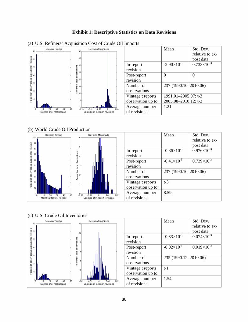
30

Exhibit 1: Descriptive Statistics on Data Revisions

(a) U.S. Refiners’ Acquisition Cost of Crude Oil Imports Mean Std. Dev.

relative to ex-post data

In-report revision

-2.90×10-3 0.733×10-3

Post-report revision

0 0

Number of observations

237 (1990.10–2010.06)

Vintage t reports observation up to

1991.01–2005.07: t-3 2005.08–2010.12: t-2

Average number of revisions

1.21

(b) World Crude Oil Production Mean Std. Dev.


In-report revision

-0.86×10-3 0.976×10-3


-0.41×10-3 0.729×10-3


237 (1990.10–2010.06)


t-3


8.59

(c) U.S. Crude Oil Inventories Mean Std. Dev.


In-report revision

-0.33×10-3 0.074×10-3


-0.02×10-3 0.019×10-3


235 (1990.12–2010.06)


t-1


1.54

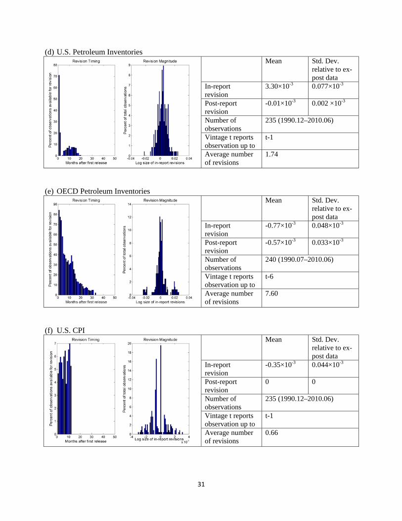
31

(d) U.S. Petroleum Inventories Mean Std. Dev.


In-report revision

3.30×10-3 0.077×10-3


-0.01×10-3 0.002 ×10-3


235 (1990.12–2010.06)


t-1


1.74

(e) OECD Petroleum Inventories Mean Std. Dev.


In-report revision

-0.77×10-3 0.048×10-3


-0.57×10-3 0.033×10-3


240 (1990.07–2010.06)


t-6


7.60

(f) U.S. CPI Mean Std. Dev.


In-report revision

-0.35×10-3 0.044×10-3


0 0


235 (1990.12–2010.06)


t-1


0.66

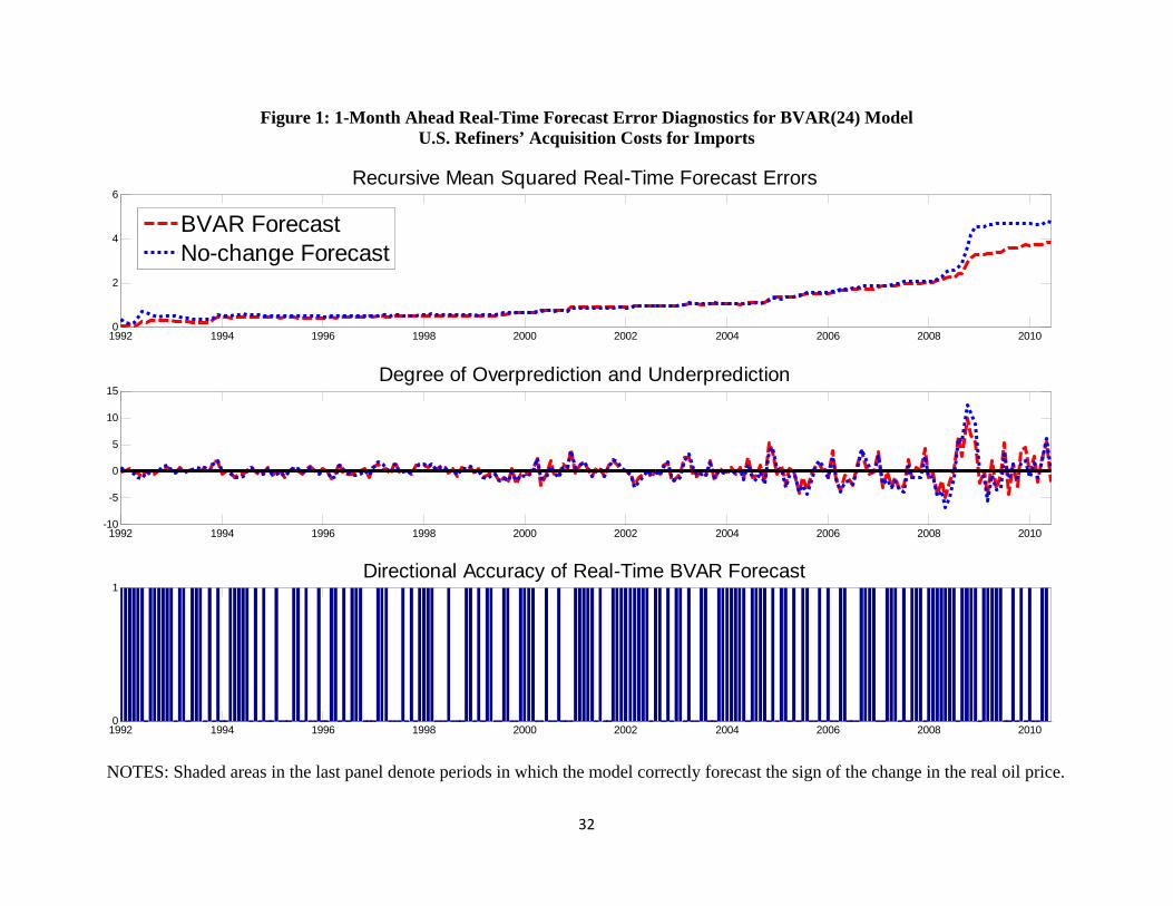
32

1992 1994 1996 1998 2000 2002 2004 2006 2008 20100

2

4

6Recursive Mean Squared Real-Time Forecast Errors

BVAR ForecastNo-change Forecast

1992 1994 1996 1998 2000 2002 2004 2006 2008 2010-10

-5

0

5

10

15Degree of Overprediction and Underprediction

1992 1994 1996 1998 2000 2002 2004 2006 2008 20100

1Directional Accuracy of Real-Time BVAR Forecast

Figure 1: 1-Month Ahead Real-Time Forecast Error Diagnostics for BVAR(24) Model U.S. Refiners’ Acquisition Costs for Imports

NOTES: Shaded areas in the last panel denote periods in which the model correctly forecast the sign of the change in the real oil price.

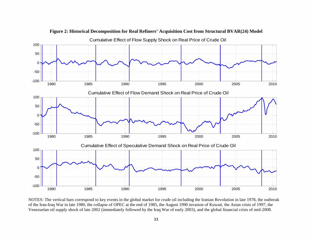
33

1980 1985 1990 1995 2000 2005 2010-100

-50

0

50

100Cumulative Effect of Flow Supply Shock on Real Price of Crude Oil

1980 1985 1990 1995 2000 2005 2010-100

-50

0

50

100Cumulative Effect of Flow Demand Shock on Real Price of Crude Oil

1980 1985 1990 1995 2000 2005 2010-100

-50

0

50

100Cumulative Effect of Speculative Demand Shock on Real Price of Crude Oil

Figure 2: Historical Decomposition for Real Refiners’ Acquisition Cost from Structural BVAR(24) Model

NOTES: The vertical bars correspond to key events in the global market for crude oil including the Iranian Revolution in late 1978, the outbreak of the Iran-Iraq War in late 1980, the collapse of OPEC at the end of 1985, the August 1990 invasion of Kuwait, the Asian crisis of 1997, the Venezuelan oil supply shock of late 2002 (immediately followed by the Iraq War of early 2003), and the global financial crisis of mid-2008.

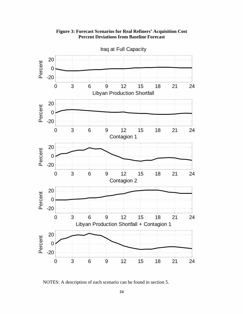
34

0 3 6 9 12 15 18 21 24

-20

0

20

Iraq at Full Capacity

Per

cent

0 3 6 9 12 15 18 21 24

-20

0

20

Libyan Production Shortfall

Per

cent

0 3 6 9 12 15 18 21 24

-20

0

20

Contagion 1

Per

cent

0 3 6 9 12 15 18 21 24

-20

0

20

Contagion 2

Per

cent

0 3 6 9 12 15 18 21 24

-20

0

20

Libyan Production Shortfall + Contagion 1

Per

cent

Figure 3: Forecast Scenarios for Real Refiners’ Acquisition Cost Percent Deviations from Baseline Forecast

NOTES: A description of each scenario can be found in section 5.

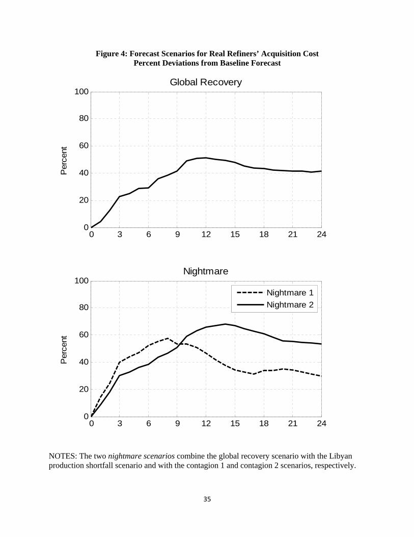
35

0 3 6 9 12 15 18 21 240

20

40

60

80

100Global Recovery

Per

cent

0 3 6 9 12 15 18 21 240

20

40

60

80

100Nightmare

Per

cent

Nightmare 1

Nightmare 2

Figure 4: Forecast Scenarios for Real Refiners’ Acquisition Cost Percent Deviations from Baseline Forecast

NOTES: The two nightmare scenarios combine the global recovery scenario with the Libyan production shortfall scenario and with the contagion 1 and contagion 2 scenarios, respectively.

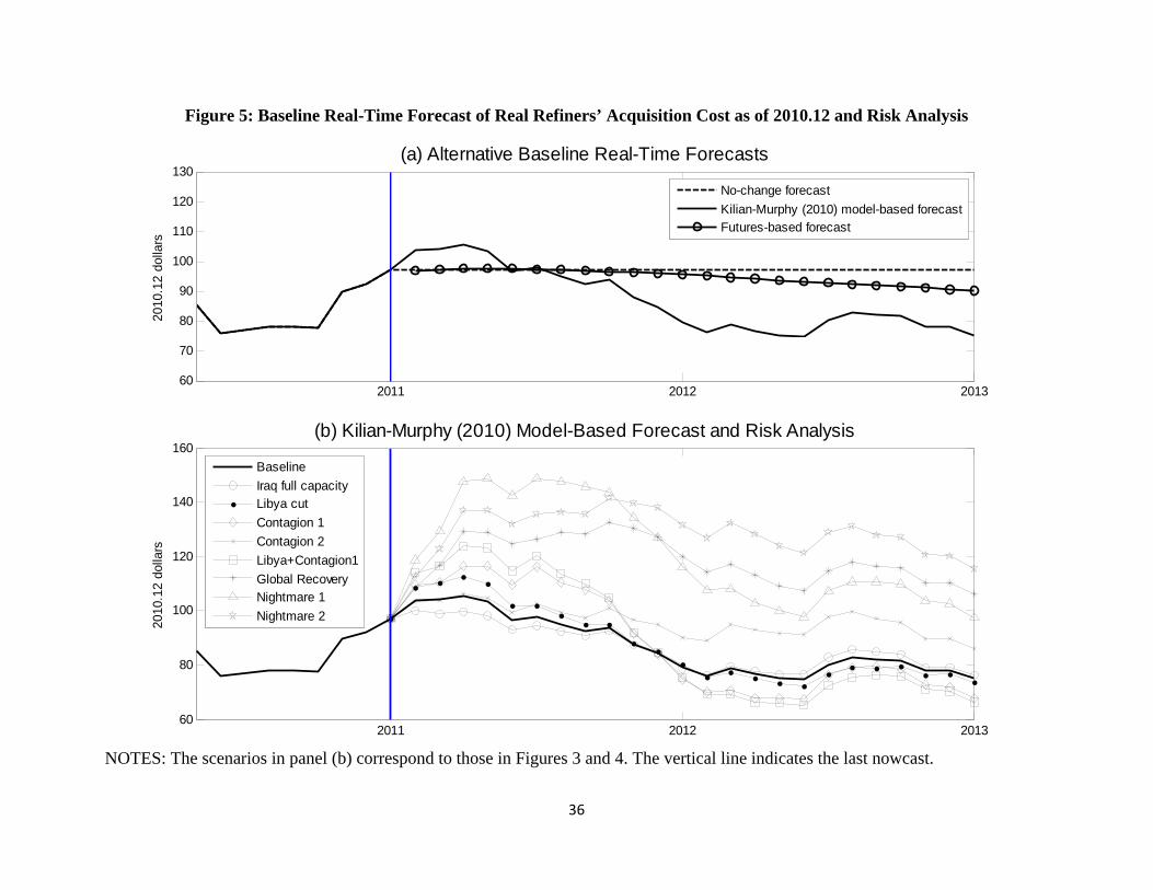
36

2011 2012 201360

70

80

90

100

110

120

13020

10.1

2 do

llars

(a) Alternative Baseline Real-Time Forecasts

No-change forecast

Kilian-Murphy (2010) model-based forecastFutures-based forecast

2011 2012 201360

80

100

120

140

160

2010

.12

dolla

rs

(b) Kilian-Murphy (2010) Model-Based Forecast and Risk Analysis

Baseline

Iraq full capacityLibya cut

Contagion 1

Contagion 2

Libya+Contagion1

Global RecoveryNightmare 1

Nightmare 2

Figure 5: Baseline Real-Time Forecast of Real Refiners’ Acquisition Cost as of 2010.12 and Risk Analysis

NOTES: The scenarios in panel (b) correspond to those in Figures 3 and 4. The vertical line indicates the last nowcast.

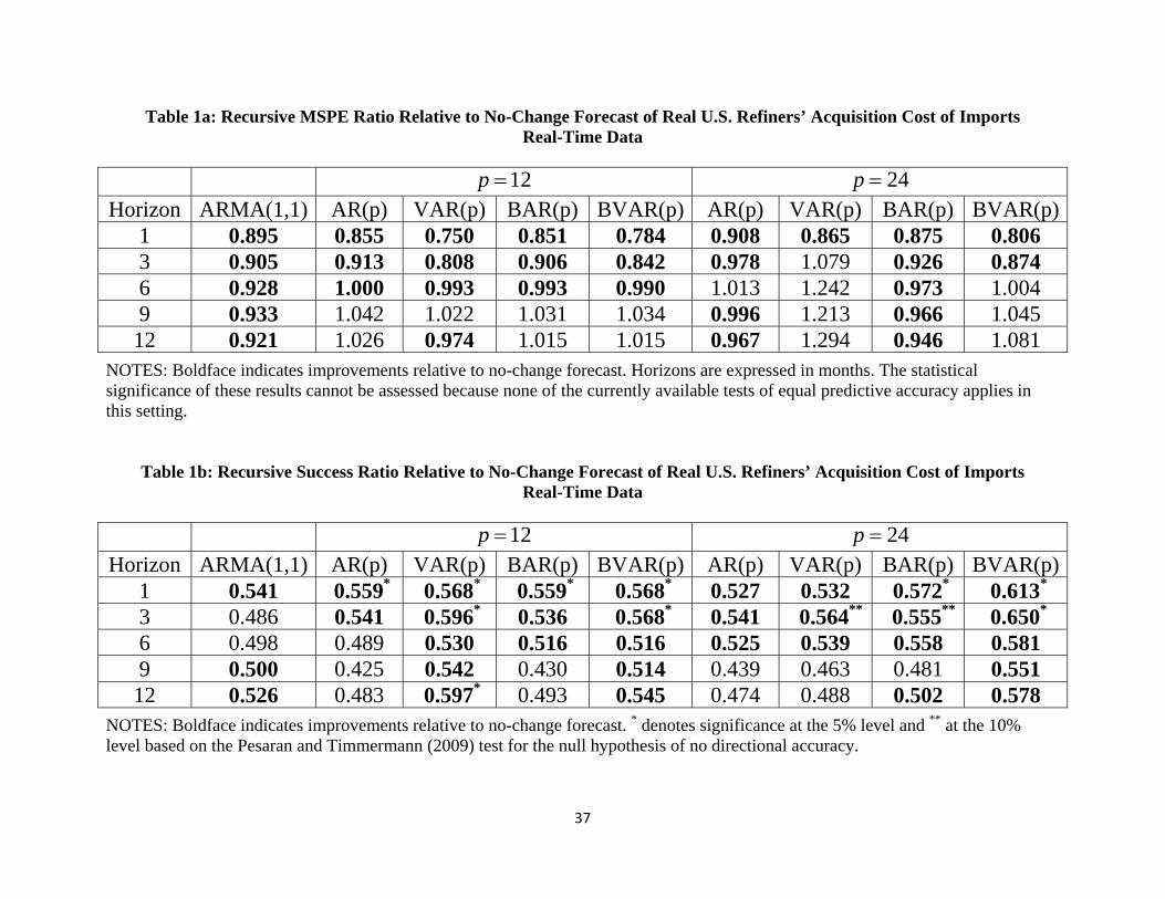
37

Table 1a: Recursive MSPE Ratio Relative to No-Change Forecast of Real U.S. Refiners’ Acquisition Cost of Imports Real-Time Data

12p 24p

Horizon ARMA(1,1) AR(p) VAR(p) BAR(p) BVAR(p) AR(p) VAR(p) BAR(p) BVAR(p)1 0.895 0.855 0.750 0.851 0.784 0.908 0.865 0.875 0.806 3 0.905 0.913 0.808 0.906 0.842 0.978 1.079 0.926 0.874 6 0.928 1.000 0.993 0.993 0.990 1.013 1.242 0.973 1.004 9 0.933 1.042 1.022 1.031 1.034 0.996 1.213 0.966 1.045

12 0.921 1.026 0.974 1.015 1.015 0.967 1.294 0.946 1.081

NOTES: Boldface indicates improvements relative to no-change forecast. Horizons are expressed in months. The statistical significance of these results cannot be assessed because none of the currently available tests of equal predictive accuracy applies in this setting.

Table 1b: Recursive Success Ratio Relative to No-Change Forecast of Real U.S. Refiners’ Acquisition Cost of Imports Real-Time Data

12p 24p

Horizon ARMA(1,1) AR(p) VAR(p) BAR(p) BVAR(p) AR(p) VAR(p) BAR(p) BVAR(p)1 0.541 0.559* 0.568* 0.559* 0.568* 0.527 0.532 0.572* 0.613*

3 0.486 0.541 0.596* 0.536 0.568* 0.541 0.564** 0.555** 0.650*

6 0.498 0.489 0.530 0.516 0.516 0.525 0.539 0.558 0.581 9 0.500 0.425 0.542 0.430 0.514 0.439 0.463 0.481 0.551

12 0.526 0.483 0.597* 0.493 0.545 0.474 0.488 0.502 0.578

NOTES: Boldface indicates improvements relative to no-change forecast. * denotes significance at the 5% level and ** at the 10% level based on the Pesaran and Timmermann (2009) test for the null hypothesis of no directional accuracy.

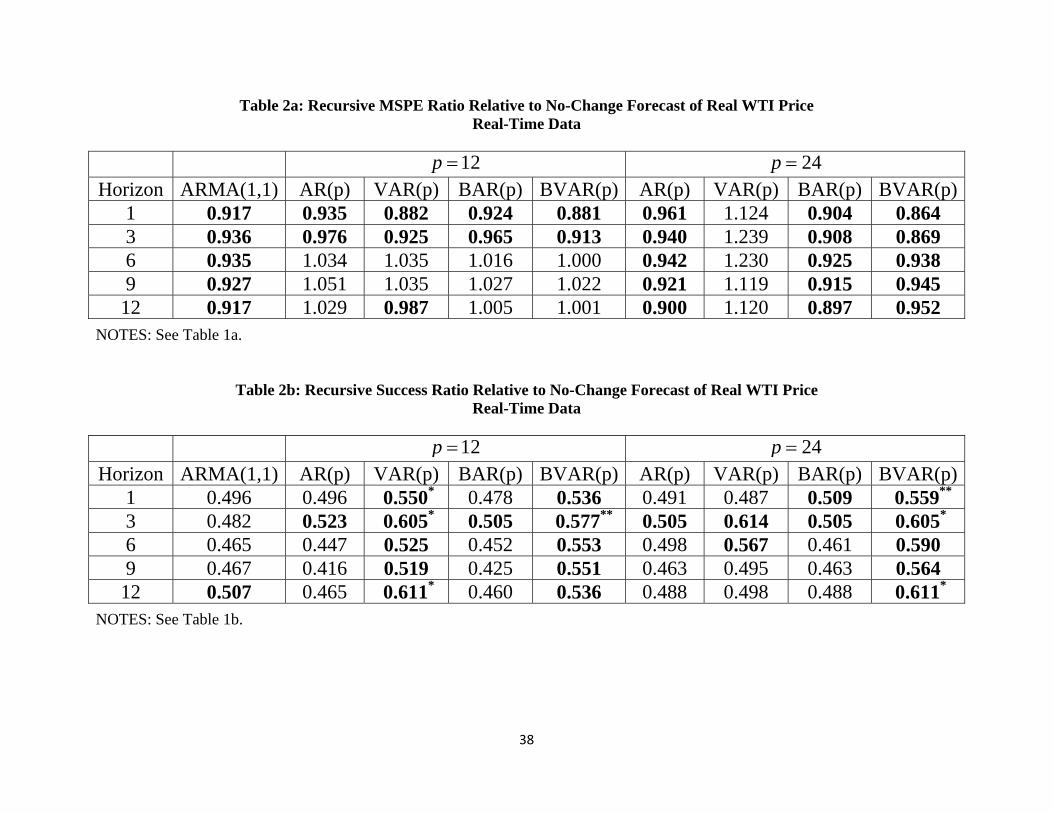
38

Table 2a: Recursive MSPE Ratio Relative to No-Change Forecast of Real WTI Price Real-Time Data

12p 24p

Horizon ARMA(1,1) AR(p) VAR(p) BAR(p) BVAR(p) AR(p) VAR(p) BAR(p) BVAR(p)1 0.917 0.935 0.882 0.924 0.881 0.961 1.124 0.904 0.864 3 0.936 0.976 0.925 0.965 0.913 0.940 1.239 0.908 0.869 6 0.935 1.034 1.035 1.016 1.000 0.942 1.230 0.925 0.938 9 0.927 1.051 1.035 1.027 1.022 0.921 1.119 0.915 0.945

12 0.917 1.029 0.987 1.005 1.001 0.900 1.120 0.897 0.952

NOTES: See Table 1a.

Table 2b: Recursive Success Ratio Relative to No-Change Forecast of Real WTI Price Real-Time Data

12p 24p

Horizon ARMA(1,1) AR(p) VAR(p) BAR(p) BVAR(p) AR(p) VAR(p) BAR(p) BVAR(p)1 0.496 0.496 0.550* 0.478 0.536 0.491 0.487 0.509 0.559**

3 0.482 0.523 0.605* 0.505 0.577** 0.505 0.614 0.505 0.605*

6 0.465 0.447 0.525 0.452 0.553 0.498 0.567 0.461 0.590 9 0.467 0.416 0.519 0.425 0.551 0.463 0.495 0.463 0.564

12 0.507 0.465 0.611* 0.460 0.536 0.488 0.498 0.488 0.611*

NOTES: See Table 1b.

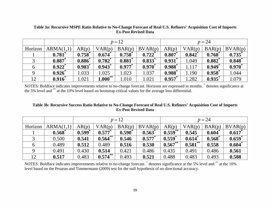
39

Table 3a: Recursive MSPE Ratio Relative to No-Change Forecast of Real U.S. Refiners’ Acquisition Cost of Imports Ex-Post Revised Data

12p 24p

Horizon ARMA(1,1) AR(p) VAR(p) BAR(p) BVAR(p) AR(p) VAR(p) BAR(p) BVAR(p)1 0.781* 0.758* 0.674* 0.758* 0.722* 0.807* 0.842* 0.768* 0.735* 3 0.887* 0.886* 0.782* 0.881* 0.833* 0.931* 1.049 0.882* 0.848* 6 0.922* 0.983* 0.943* 0.977* 0.970* 0.988* 1.117 0.949* 0.970* 9 0.926* 1.033 1.025 1.023 1.037 0.988* 1.190 0.958* 1.044

12 0.916* 1.021 1.000** 1.010 1.021 0.957* 1.282 0.935* 1.079

NOTES: Boldface indicates improvements relative to no-change forecast. Horizons are expressed in months. * denotes significance at the 5% level and ** at the 10% level based on bootstrap critical values for the average loss differential.

Table 3b: Recursive Success Ratio Relative to No-Change Forecast of Real U.S. Refiners’ Acquisition Cost of Imports Ex-Post Revised Data

12p 24p

Horizon ARMA(1,1) AR(p) VAR(p) BAR(p) BVAR(p) AR(p) VAR(p) BAR(p) BVAR(p)1 0.568* 0.599* 0.577* 0.590* 0.563* 0.559** 0.545 0.604* 0.617*

3 0.500 0.541 0.564** 0.546 0.577* 0.559* 0.614* 0.568* 0.659*

6 0.489 0.512 0.489 0.516 0.530 0.567** 0.581** 0.558 0.604*

9 0.491 0.430 0.514 0.421 0.486 0.435 0.491 0.486 0.561 12 0.517 0.483 0.574** 0.493 0.521 0.488 0.483 0.493 0.588

NOTES: Boldface indicates improvements relative to no-change forecast. * denotes significance at the 5% level and ** at the 10% level based on the Pesaran and Timmermann (2009) test for the null hypothesis of no directional accuracy.

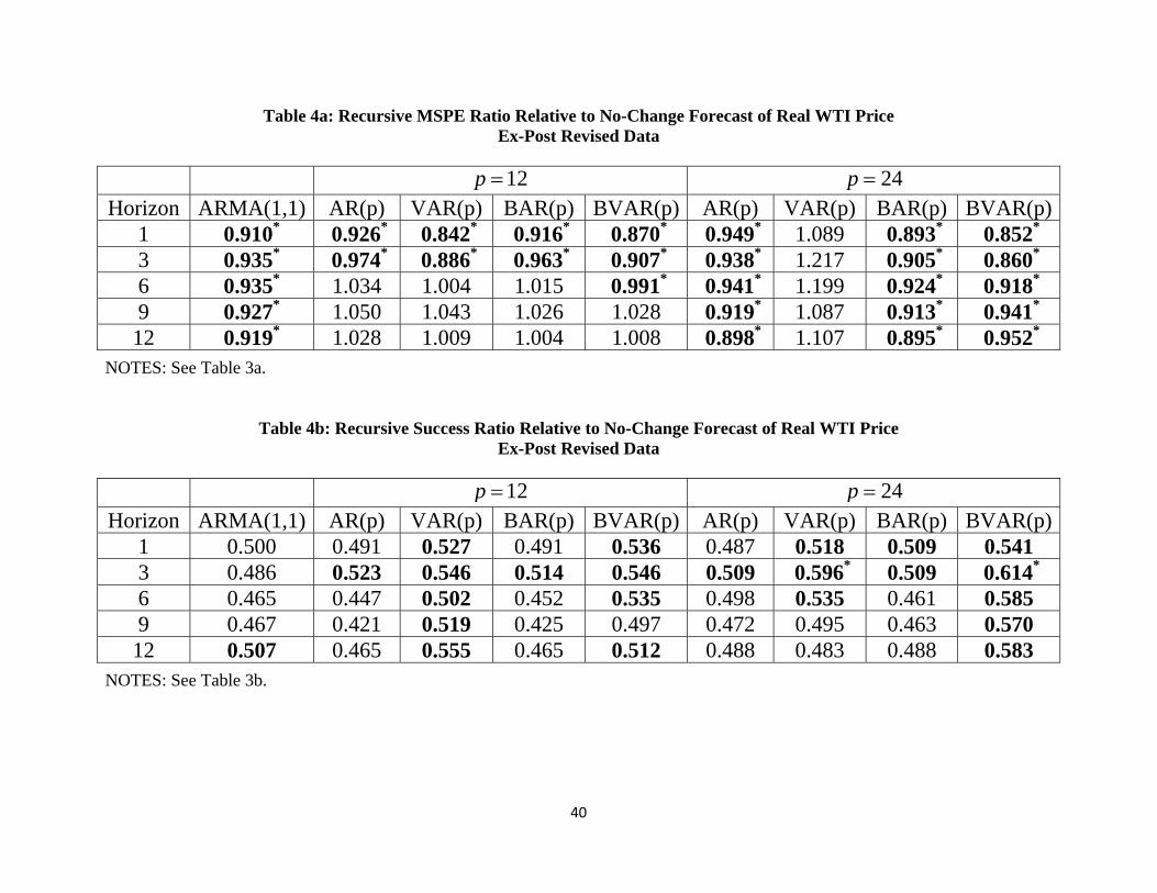
40

Table 4a: Recursive MSPE Ratio Relative to No-Change Forecast of Real WTI Price Ex-Post Revised Data

12p 24p

Horizon ARMA(1,1) AR(p) VAR(p) BAR(p) BVAR(p) AR(p) VAR(p) BAR(p) BVAR(p)1 0.910* 0.926* 0.842* 0.916* 0.870* 0.949* 1.089 0.893* 0.852* 3 0.935* 0.974* 0.886* 0.963* 0.907* 0.938* 1.217 0.905* 0.860* 6 0.935* 1.034 1.004 1.015 0.991* 0.941* 1.199 0.924* 0.918* 9 0.927* 1.050 1.043 1.026 1.028 0.919* 1.087 0.913* 0.941*

12 0.919* 1.028 1.009 1.004 1.008 0.898* 1.107 0.895* 0.952*

NOTES: See Table 3a.

Table 4b: Recursive Success Ratio Relative to No-Change Forecast of Real WTI Price Ex-Post Revised Data

12p 24p

Horizon ARMA(1,1) AR(p) VAR(p) BAR(p) BVAR(p) AR(p) VAR(p) BAR(p) BVAR(p)1 0.500 0.491 0.527 0.491 0.536 0.487 0.518 0.509 0.541 3 0.486 0.523 0.546 0.514 0.546 0.509 0.596* 0.509 0.614*

6 0.465 0.447 0.502 0.452 0.535 0.498 0.535 0.461 0.585 9 0.467 0.421 0.519 0.425 0.497 0.472 0.495 0.463 0.570

12 0.507 0.465 0.555 0.465 0.512 0.488 0.483 0.488 0.583

NOTES: See Table 3b.

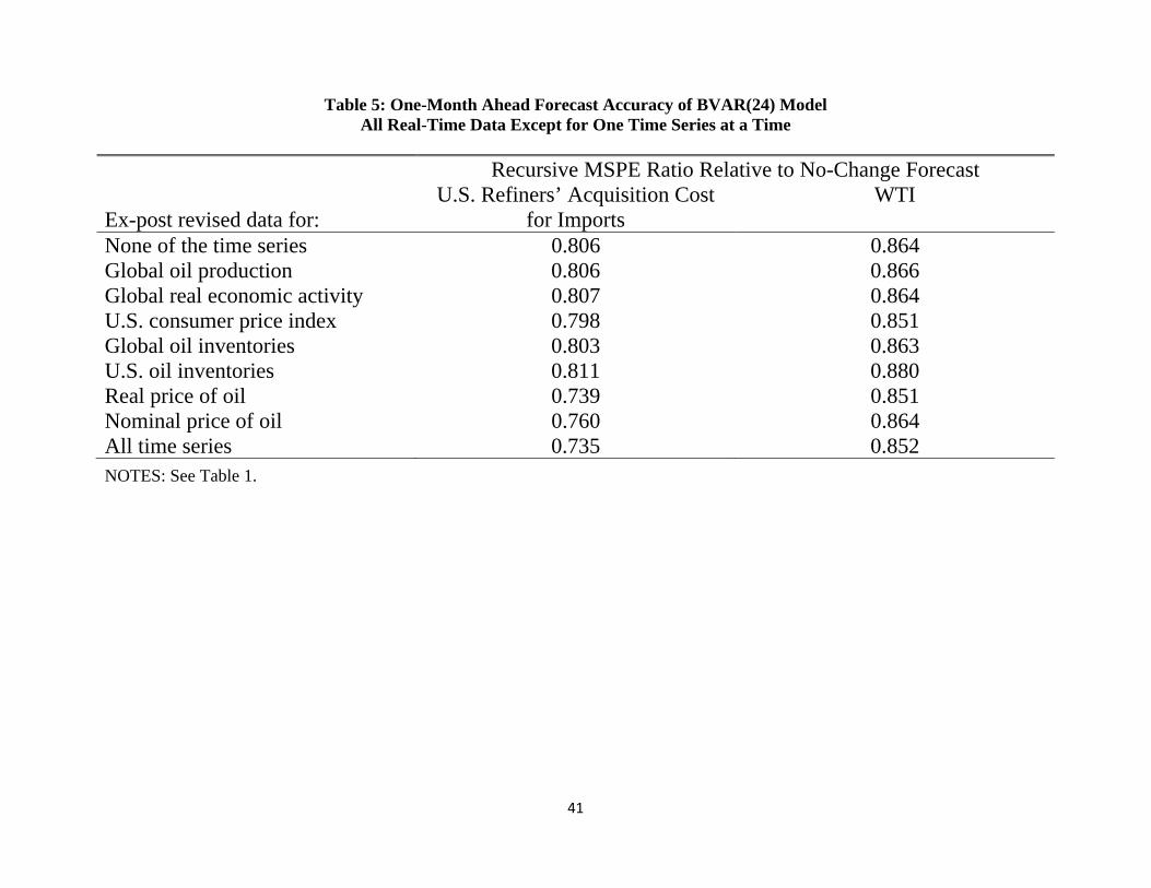
41

Table 5: One-Month Ahead Forecast Accuracy of BVAR(24) Model All Real-Time Data Except for One Time Series at a Time

Recursive MSPE Ratio Relative to No-Change Forecast Ex-post revised data for:

U.S. Refiners’ Acquisition Cost for Imports

WTI

None of the time series 0.806 0.864 Global oil production 0.806 0.866 Global real economic activity 0.807 0.864 U.S. consumer price index 0.798 0.851 Global oil inventories 0.803 0.863 U.S. oil inventories 0.811 0.880 Real price of oil 0.739 0.851 Nominal price of oil 0.760 0.864 All time series 0.735 0.852

NOTES: See Table 1.

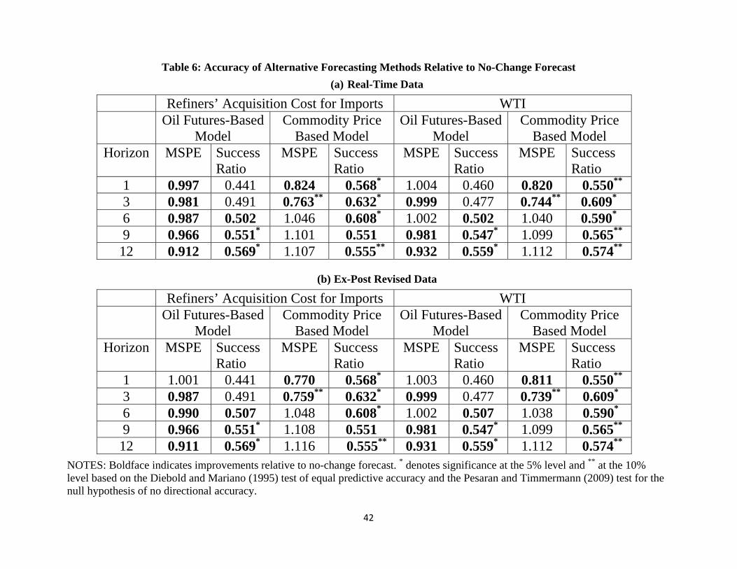
42

Table 6: Accuracy of Alternative Forecasting Methods Relative to No-Change Forecast

(a) Real-Time Data

Refiners’ Acquisition Cost for Imports WTI Oil Futures-Based

Model Commodity Price

Based Model Oil Futures-Based


Based Model Horizon MSPE Success

Ratio MSPE Success

Ratio MSPE Success

Ratio MSPE Success

Ratio 1 0.997 0.441 0.824 0.568* 1.004 0.460 0.820 0.550**

3 0.981 0.491 0.763** 0.632* 0.999 0.477 0.744** 0.609*

6 0.987 0.502 1.046 0.608* 1.002 0.502 1.040 0.590*

9 0.966 0.551* 1.101 0.551 0.981 0.547* 1.099 0.565**

12 0.912 0.569* 1.107 0.555** 0.932 0.559* 1.112 0.574**

(b) Ex-Post Revised Data

Refiners’ Acquisition Cost for Imports WTI Oil Futures-Based


Based Model Oil Futures-Based


Based Model Horizon MSPE Success

Ratio MSPE Success

Ratio MSPE Success

Ratio MSPE Success

Ratio 1 1.001 0.441 0.770 0.568* 1.003 0.460 0.811 0.550**

3 0.987 0.491 0.759** 0.632* 0.999 0.477 0.739** 0.609*

6 0.990 0.507 1.048 0.608* 1.002 0.507 1.038 0.590*

9 0.966 0.551* 1.108 0.551 0.981 0.547* 1.099 0.565**

12 0.911 0.569* 1.116 0.555** 0.931 0.559* 1.112 0.574**

NOTES: Boldface indicates improvements relative to no-change forecast. * denotes significance at the 5% level and ** at the 10% level based on the Diebold and Mariano (1995) test of equal predictive accuracy and the Pesaran and Timmermann (2009) test for the null hypothesis of no directional accuracy.

Real-Time Forecasts of the Real Price of Oil - frbsf.org · Real-Time Forecasts of the Real Price...

Documents

Transcript of Real-Time Forecasts of the Real Price of Oil - frbsf.org · Real-Time Forecasts of the Real Price...