WP/14/218

Oil Price Volatility and the Role of Speculation

Samya Beidas-Strom and Andrea Pescatori

© 2014 International Monetary Fund WP/14/218

IMF Working Paper

Research Department

Oil Price Volatility and the Role of Speculation

Prepared by Samya Beidas-Strom and Andrea Pescatori

Authorized for distribution by Thomas Helbling

December 2014

Abstract

How much does speculation contribute to oil price volatility? We revisit this contentious

question by estimating a sign-restricted structural vector autoregression (SVAR). First,

using a simple storage model, we show that revisions to expectations regarding oil market

fundamentals and the effect of mispricing in oil derivative markets can be observationally

equivalent in a SVAR model of the world oil market à la Kilian and Murphy (2013), since

both imply a positive co-movement of oil prices and inventories. Second, we impose

additional restrictions on the set of admissible models embodying the assumption that the

impact from noise trading shocks in oil derivative markets is temporary. Our additional

restrictions effectively put a bound on the contribution of speculation to short-term oil price

volatility (lying between 3 and 22 percent). This estimated short-run impact is smaller than

that of flow demand shocks but possibly larger than that of flow supply shocks.

JEL Classification Numbers: E32, D84, F02, Q41, Q43, Q48

Keywords: oil and the business cycle; crude oil speculation and inventories; demand and supply

shocks; oil price volatility; vector autoregression (VAR)

Authors’ E-Mail Addresses: sbeidasstrom@imf.org; apescatori@imf.org

IMF Working Papers describe research in progress by the authors and are published to elicit

comments and to encourage debate. The views expressed in IMF Working Paper are those of the

authors and do not necessarily represent the views of the IMF, its Executive Board or IMF

Management.

2

Contents Page

I. Introduction .......................................................................................................................3

II. Literature Review..............................................................................................................6

III. A Storage Model of Speculation .......................................................................................8

IV. An Estimated VAR Model of the Global Oil Market .....................................................13

A. Data ........................................................................................................................13

B. Model Specification ...............................................................................................14

C. Estimation Methodology and Identification ..........................................................15

D. When Does Speculative Demand Matter? .............................................................18

V. Conclusion ......................................................................................................................23

Figures

1. Evolution of the Real Oil Price and Political Events ........................................................3

2. Admissible Estimated Models–Impulse Response Functions ........................................17

3. Narrowing the Admissible Estimated Models–IRFs ......................................................19

4. Historical Decomposition of the Drivers of the Real Oil Price ......................................22

5. Absolute Drivers of the Real Oil Price ...........................................................................22

Tables

1. Real Oil Price Variance Decomposition .........................................................................20

References ................................................................................................................................25

Appendix ..................................................................................................................................28

3

I. INTRODUCTION1

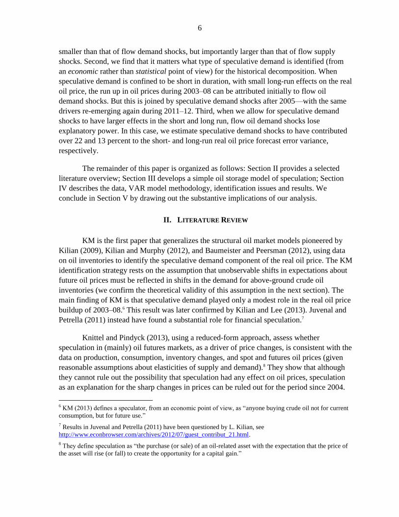
In a seminal contribution, Kilian (2009) broke with the tradition of assuming most oil

price changes reflect exogenous supply shocks, emphasizing that fluctuations in global crude

oil spot prices also reflect global economic conditions (Figure 1).2 Using a structural vector

auto regression (SVAR), he showed that global flow supply shocks have actually contributed

very little to oil price movements when compared to global flow demand shocks, especially

in the last decade. A question that naturally arises, though, is whether flow oil production and

flow demand alone can span the entire spectrum of factors that can drive the real price of oil.

If storing oil were prohibitively expensive (both above and below ground) then the

answer to the above question would be yes, since the only forces able to determine the oil

price would in that case be captured by current demand and production conditions. However,

since it is possible to store oil, changes in oil inventories are possibly a third driver behind oil

price fluctuations. Of particular interest are changes in the demand for inventories arising

1 We thank Christiane Baumeister, Olivier Blanchard, Olivier Coibion, Jörg Decressin, Thomas Helbling, and

Lutz Kilian (for suggestions on an earlier draft); Daniel Rivera Greenwood and Marina Rousset (for research

assistance); Michael Harrup and Anduriña Espinoza-Wasil (for editorial and administrative assistance,

respectively); and RES seminar participants (for helpful discussions). Without implication, we are grateful for

oil-market insights from: Fatih Birol, John Brunton, Bassam Fattouh, David Fyfe, Fabio Gabrieli, Antione

Halff, Daniel Jaeggi, Olivier Jakob, Giles Jones, Jason Lejonvarn, Benoit Lioud, Donal O’Shea, Amrita Sen,

and Joerg Spitzy. The usual disclaimer applies.

2 In a theoretical context, Backus and Crucini (2000) and Nakov and Pescatori (2010) also highlighted the

importance of distinguishing the source of shocks behind oil price movements.

0

10

20

30

40

50

60

70

80

90

100

85Q2 88Q2 91Q2 94Q2 97Q2 00Q2 03Q2 06Q2 09Q2 12Q2

Figure 1. Evolution of the Real Oil Price and Political Events

12Q4

Following high prices of the Iraq-Iran war (1980), Saudi abandons

OPEC swing producer role

Iraq invades Kuwait

Asian financial

crisis

OPEC cutsproduction (1.7 mbd)

Sep.11attack

Venezuela coup, followed by

unrest in Nigeria and the Iraq war

Hurricane Katrina

Lehman collapse

OPEC cuts

production (4.2 mbd)

Libyan civil war,followed

byArab

Spring

Sources: IMF, Primary Commodity Price System; IMF Global Data Source. Note: The nominal price is deflated by the US CPI, 2010=100.

4

from speculative motives, that is, changes driven by expectations of future price changes.3

Indeed, Kilian and Murphy (2013) have extended the Kilian (2009) model, identifying

speculative demand shocks and including oil inventories as an additional variable.

In a rational expectations world, speculation reflects the forward-looking nature of

economic agents who manage inventories to smooth their oil consumption and production

over time—paying attention to the expected future path of the oil price. Moreover, in a

rational expectations world, such speculation helps to stabilize spot prices when there are

temporary demand or supply shocks. For example, if spot prices rise (fall) because flow

production (demand) temporarily drops due to a supply (demand) shock, inventory holders

can realize profits by selling (buying) stocks, which they can replenish (sell) later at a lower

(higher) price. This release (stocking up) of inventories will increase (decrease) the effective

supply in the market, which in turn will dampen (push up) the spot price response to the

supply (demand) shock.

From this vantage point, speculative demand simply represents rational decisions of

adjusting above-the-ground holdings of oil inventories in anticipation of price movements as

new information arrives on future market conditions. In other words, economic agents

manage inventories to smooth their oil consumption and production over time, given the

expected future path of the oil price. Changes in speculative demand are therefore a response

to expected changes in oil market fundamentals—also known as news shocks (à la Jaimovich

and Rebelo, 2009), such as oil discoveries, expectations of production disruptions, backstop

technologies, and changes in world real interest rates or in global demand growth.4

In recent years, however, there have been strong concerns that the emergence of

commodity derivatives as an asset class has led to destabilizing speculation. In the Kilian and

Murphy (2013) model, this concern would manifest itself in destabilizing shocks to inventory

demand. In other words, the claim would be that inventory demand has responded to changes

in oil futures prices that are not firmly grounded in new information about future oil market

fundamentals, including changes in economic activity. Or differently put, oil futures prices,

similar to other commodity futures prices, have reflected a greater incidence of noise trading

or other anomalies (à la Fama, 1998; and Singleton, 2011). Such concerns about destabilizing

speculation have been a constant refrain in recent years despite the lack of conclusive

supporting evidence (IMF, 2011b; Fattouh, Killian and Mahadeva, 2012; Büyükşahin and

Robe, 2012; Knittel and Pindyck, 2013; and Kilian and Lee, 2013).

3 In addition to speculation, oil-specific demand shocks may affect oil prices. Even though these shocks are

captured in our framework, they will not be at the center of our discussion.

4 It is important to clarify that “news” has been used in the finance literature to mean the difference between

expectations and outcomes. For example, Kilian and Vega (2011) test whether oil prices react to

macroeconomic news from U.S. data releases, where macroeconomic news is defined as the difference between

ex ante survey expectations and the subsequently announced realizations of macroeconomic aggregates.

5

In this paper, we attempt to explore the short-term effects of speculative oil demand

shocks studied by Kilian and Murphy (2013) (henceforth KM) in greater detail. Using their

framework, we cannot distinguish between speculative demand shocks driven by news about

fundamentals and those driven by noise trading. However, we further narrow the set of

admissible models by limiting the contribution of speculative demand shocks to the long-run

oil price forecast error variance (in addition to the restrictions used in KM). In other words,

we seek to identify a range for the response of oil prices (i.e., oil price volatility) to

speculative demand shocks by imposing restrictions on the time horizon in which noise

trading and other factors affect oil markets.

The rationale for our additional restrictions is as follows: while we cannot a priori

exclude noise trading and other anomalies in oil futures markets in times of rapid structural

change, we can plausibly assume that such anomalies will not last. Arbitrage by fundamental

traders should ensure that prices are in line with fundamentals. Specifically, our null

hypothesis is that only oil market fundamentals (or news about them) can induce low-

frequency movements in oil prices. To be more concrete, oil discoveries (which have long

lags before coming on stream) or revisions to potential growth of major economies (e.g.,

China, Japan, or the United States) must have a very persistent effect on the oil price. Under

the null hypothesis, mispricing in the futures market (i.e., noise trading by financial

speculators) is a temporary anomaly that does not contribute to low-frequency price

movements. Therefore, it is possible to set a bound on its contribution to oil price volatility

by restricting our attention to the admissible model that minimizes the oil price forecast error

variance contribution of speculative shocks at long horizons (i.e., 20 years). Furthermore,

even though other fundamental shocks may have only temporary effects on oil prices (for

example, an anticipated temporary production shortfall), we would still be able to interpret

our results as a short-run upper bound to the role played by financial and non-financial

speculative shocks.5 Indeed, given that we employ data on crude oil inventories to estimate

this upper bound, it is actually an upper bound for the oil price response to any speculative

demand shock, regardless of its motive.

The paper’s contribution is mainly twofold. First, we show that news shocks on oil

market fundamentals, mispricing in the oil futures market, and global real interest rate shocks

can manifest themselves as speculative demand shocks under the KM identification strategy.

Second, we propose a novel manner for putting a plausible bound on the contribution of

financial speculation to short-term oil price volatility.

Our key findings are as follows. First, we find that typical speculative demand shocks

in the crude oil market may increase or decrease the real oil price on impact between 10 and

35 percent, contributing to short-run oil price volatility. This estimated short-run impact is

5 As a corollary, for a temporary demand weakness, we would find a short-run lower bound to the role played

by financial and non-financial speculative shocks.

6

smaller than that of flow demand shocks, but importantly larger than that of flow supply

shocks. Second, we find that it matters what type of speculative demand is identified (from

an economic rather than statistical point of view) for the historical decomposition. When

speculative demand is confined to be short in duration, with small long-run effects on the real

oil price, the run up in oil prices during 2003–08 can be attributed initially to flow oil

demand shocks. But this is joined by speculative demand shocks after 2005—with the same

drivers re-emerging again during 2011–12. Third, when we allow for speculative demand

shocks to have larger effects in the short and long run, flow oil demand shocks lose

explanatory power. In this case, we estimate speculative demand shocks to have contributed

over 22 and 13 percent to the short- and long-run real oil price forecast error variance,

respectively.

The remainder of this paper is organized as follows: Section II provides a selected

literature overview; Section III develops a simple oil storage model of speculation; Section

IV describes the data, VAR model methodology, identification issues and results. We

conclude in Section V by drawing out the substantive implications of our analysis.

II. LITERATURE REVIEW

KM is the first paper that generalizes the structural oil market models pioneered by

Kilian (2009), Kilian and Murphy (2012), and Baumeister and Peersman (2012), using data

on oil inventories to identify the speculative demand component of the real oil price. The KM

identification strategy rests on the assumption that unobservable shifts in expectations about

future oil prices must be reflected in shifts in the demand for above-ground crude oil

inventories (we confirm the theoretical validity of this assumption in the next section). The

main finding of KM is that speculative demand played only a modest role in the real oil price

buildup of 2003–08.6 This result was later confirmed by Kilian and Lee (2013). Juvenal and

Petrella (2011) instead have found a substantial role for financial speculation.7

Knittel and Pindyck (2013), using a reduced-form approach, assess whether

speculation in (mainly) oil futures markets, as a driver of price changes, is consistent with the

data on production, consumption, inventory changes, and spot and futures oil prices (given

reasonable assumptions about elasticities of supply and demand).8 They show that although

they cannot rule out the possibility that speculation had any effect on oil prices, speculation

as an explanation for the sharp changes in prices can be ruled out for the period since 2004.

6 KM (2013) defines a speculator, from an economic point of view, as “anyone buying crude oil not for current

consumption, but for future use.”

7 Results in Juvenal and Petrella (2011) have been questioned by L. Kilian, see

http://www.econbrowser.com/archives/2012/07/guest_contribut_21.html.

8 They define speculation as “the purchase (or sale) of an oil-related asset with the expectation that the price of

the asset will rise (or fall) to create the opportunity for a capital gain.”

7

They argue that, unless one believes that the price elasticities of both oil supply and demand

are close to zero (a conjecture initially put forward by Hamilton, 2009), the behavior of

inventories and futures-spot spreads are simply inconsistent with the view that speculation

was a significant driver of spot prices over that period. Across their sample, speculation

decreased prices on average or left them essentially unchanged and reduced peak prices by

roughly 5 percent.

A common feature of the above papers is that their definition of speculation does not

distinguish whether it is related to fundamentals or not—or, more generally, what induces

speculative demand shocks.

Another strand of the literature has instead focused on a narrower definition of

speculation which is mainly related to the possible malfunctioning of commodity financial

derivative markets (à la Fama, 1998). Masters (2008) blames the oil price spike of 2007–08

on the actions of investors who bought oil futures not as a commodity to use but as a

financial asset. He argues that by March 2008, commodity index trading funds (ITFs)

holding a quarter of a trillion U.S. dollars’ worth of futures contracts were able to push the

spot price up dramatically—however, no coherent testable model is provided. Alquist and

Kilian (2010), Liu and Tang (2010), and Tang and Xiong (2010) find a structural break in the

spot oil price post-2004. The latter attribute it to institutional investors entering the futures

market, which then led the spot price to rise higher, moving more closely with the “risk

premium” of the stock market.

To rationalize deviations from fundamentals, Singleton (2011) evokes the beauty

contest of Keynes, stressing that participants in oil futures markets may form expectations

not only in terms of expected fundamentals, but also in anticipation of other market

participants’ actions.9 He explores the impact of “active” investor flows and financial market

conditions on returns in crude oil futures markets. Singleton (2011) shows how financial and

informational frictions and the associated speculative activity induce prices to drift away

from “fundamentals” and thus show increased volatility. He finds significant empirical

support that financial activities are likely to drive the spot oil price away from fundamental

values, primarily through investor flows influencing excess returns from holding oil futures

contracts of different maturities. Various micro studies using confidential data of the

Commodities Future Trading Commission, however, have struggled to find evidence that

9 This builds on earlier studies that showed that heterogeneity of expectations leads investors to overweigh

public opinion and this, in turn, exacerbates volatility in financial markets. In addition to excessive volatility,

differences of opinion can give rise to drifts in commodity prices and momentum-like trading (herding) in

response to public announcements. Likewise, there is a concern that some market participants may overreact to

or misinterpret public information or signals that do not reflect large changes in underlying fundamentals. This

concern seems particularly pertinent when new market participants lack the expertise to understand oil market

developments.

8

non-commercial players have been able to influence oil (or more generally, commodity)

price movements (e.g., Büyükşahin and Robe, 2012).

III. A STORAGE MODEL OF SPECULATION

In this section we present a simple storage model of the oil market, in the spirit of

Scheinkman and Schechtman (1983), to guide our identification strategy.

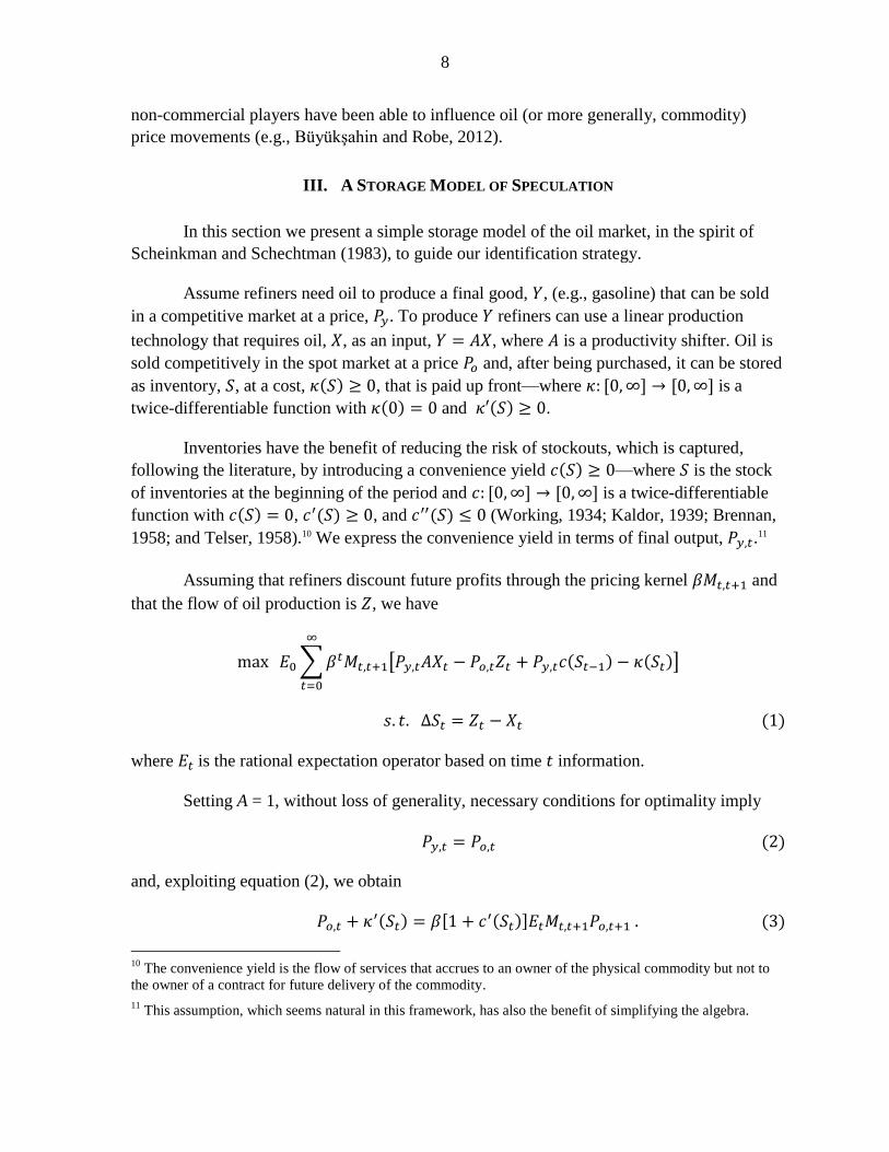
Assume refiners need oil to produce a final good, , (e.g., gasoline) that can be sold

in a competitive market at a price, . To produce refiners can use a linear production

technology that requires oil, , as an input, , where is a productivity shifter. Oil is

sold competitively in the spot market at a price and, after being purchased, it can be stored

as inventory, , at a cost, , that is paid up front—where is a

twice-differentiable function with and .

Inventories have the benefit of reducing the risk of stockouts, which is captured,

following the literature, by introducing a convenience yield —where is the stock

of inventories at the beginning of the period and is a twice-differentiable

function with , , and (Working, 1934; Kaldor, 1939; Brennan,

1958; and Telser, 1958).10 We express the convenience yield in terms of final output, .11

Assuming that refiners discount future profits through the pricing kernel and

that the flow of oil production is , we have

where is the rational expectation operator based on time information.

Setting A = 1, without loss of generality, necessary conditions for optimality imply

and, exploiting equation (2), we obtain

10

The convenience yield is the flow of services that accrues to an owner of the physical commodity but not to

the owner of a contract for future delivery of the commodity.

11 This assumption, which seems natural in this framework, has also the benefit of simplifying the algebra.

9

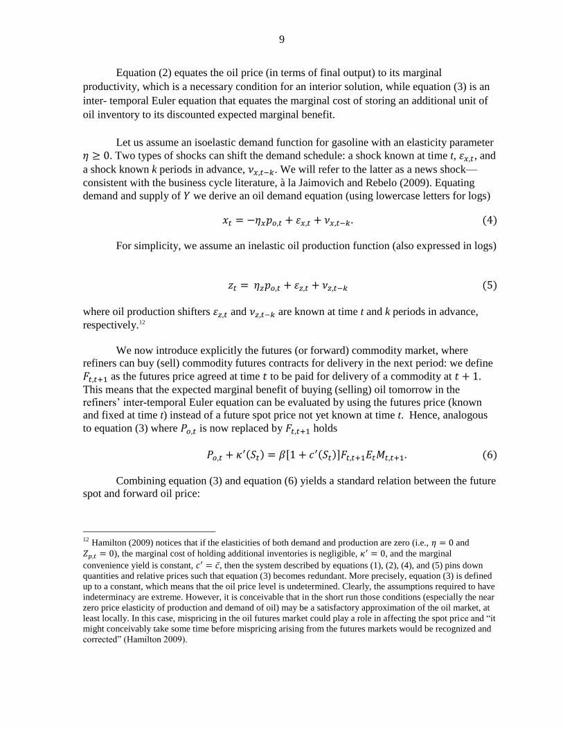
Equation (2) equates the oil price (in terms of final output) to its marginal

productivity, which is a necessary condition for an interior solution, while equation (3) is an

inter- temporal Euler equation that equates the marginal cost of storing an additional unit of

oil inventory to its discounted expected marginal benefit.

Let us assume an isoelastic demand function for gasoline with an elasticity parameter

. Two types of shocks can shift the demand schedule: a shock known at time t, , and

a shock known k periods in advance, . We will refer to the latter as a news shock—

consistent with the business cycle literature, à la Jaimovich and Rebelo (2009). Equating

demand and supply of we derive an oil demand equation (using lowercase letters for logs)

For simplicity, we assume an inelastic oil production function (also expressed in logs)

where oil production shifters and are known at time t and k periods in advance,

respectively.12

We now introduce explicitly the futures (or forward) commodity market, where

refiners can buy (sell) commodity futures contracts for delivery in the next period: we define

as the futures price agreed at time to be paid for delivery of a commodity at .

This means that the expected marginal benefit of buying (selling) oil tomorrow in the

refiners’ inter-temporal Euler equation can be evaluated by using the futures price (known

and fixed at time t) instead of a future spot price not yet known at time t. Hence, analogous

to equation (3) where is now replaced by holds

Combining equation (3) and equation (6) yields a standard relation between the future

spot and forward oil price:

12 Hamilton (2009) notices that if the elasticities of both demand and production are zero (i.e., and

), the marginal cost of holding additional inventories is negligible, , and the marginal

convenience yield is constant, , then the system described by equations (1), (2), (4), and (5) pins down

quantities and relative prices such that equation (3) becomes redundant. More precisely, equation (3) is defined

up to a constant, which means that the oil price level is undetermined. Clearly, the assumptions required to have

indeterminacy are extreme. However, it is conceivable that in the short run those conditions (especially the near

zero price elasticity of production and demand of oil) may be a satisfactory approximation of the oil market, at

least locally. In this case, mispricing in the oil futures market could play a role in affecting the spot price and “it

might conceivably take some time before mispricing arising from the futures markets would be recognized and

corrected” (Hamilton 2009).

10

Equation (7) suggests that the futures price is equal to the expected future spot price

plus a risk premium. Futures prices are, thus, determined residually from the rest of the

system, that is, equations (1)–(5), through equation (6) (or, equivalently, equation (7)). In

other words, causality does not run from futures to spot prices but runs in the opposite

direction. Loosely speaking, in this case futures prices are determined by fundamentals—that

is, there is no “mispricing.” We will refer to the system (1)–(6) as a fundamental system and

its associated variables as fundamental values which will be denoted by an asterisk, for

example, .

To introduce the possibility of deviations from fundamentals (i.e., mispricing) in the

futures market we postulate the following simple equation:

where is a stationary process that represents a shock that makes the actual futures price

deviate from its fundamental value .13 Contrary to equation (7), equation (7 ) is not a

combination of equations (3) and (6). Thus the system given by equations (1)–(6), and (7 ) is

over-identified: to have a well-identified system, we need to drop one equation. It is

reasonable to drop equation (3), which is the inter-temporal equation describing the

optimality condition of refiners. The new system, given by equations (1), (2), (4), (5), (6),

and (7 ), can no longer be split into two blocks where the futures price is determined

residually from the rest of the system.14 Loosely speaking, the no-arbitrage condition that

links the futures market to the cash market, equation (6), now describes how futures prices

can affect spot prices and inventories. When , the non-fundamental system becomes

or collapses to the fundamental system described above. This also means that the non-

fundamental system is oscillating around the fundamental system’s steady state.

13 The economic literature has highlighted various reasons that may limit arbitrage. For example, arbitrage

conditions can break down in the presence of some transaction costs or credit frictions that would ultimately

induce some forms of market segmentation (Gromb and Vayanos, 2010). In this context, market segmentation

may, on the one hand, prevent investors in the futures market from operating in the cash market, and, on the

other hand, may prevent investors in the cash market (e.g., refiners)—possibly because of liquidity constraints

or risk aversion—from arbitraging away the futures market.

14 More precisely, the overall system is formed by equations (1), (2), (4), (5), (6), and (7 ) and by the

fundamental system, equations (1)–(6), necessary to determine fundamental values, such as ; hence, the

overall system is 12 equations in 12 unknowns.

11

Interestingly, we can also write a new version of equation (3) where the spot oil price

depends on the future expected spot price plus a “wedge”, . This wedge is meant to

reflect the deviation of actual expectations of future spot prices from expectations based only

on fundamentals:

where and

is the fundamental oil price.

First, we focus on the fundamental system by setting . The (linearized)

rational expectation equilibrium can be summarized by two equations (see appendix for

details):

* * 1 111 1 1

0

* 1 *

(1 ) [ ]1

( )

j

t t t t j t j

j

ot t t

s s E

p s

where , while is a function of model’s parameters satisfying and

with and .

It is now possible to summarize the model’s predictions in terms of fundamental

shocks:

Flow supply shocks. A negative oil production shock has an unambiguous positive

effect on the oil price since . The smaller the oil price elasticity, the higher the price

impact of the flow supply shock. The impact on inventories is unambiguously negative in

case of either i.i.d. or persistent but mean-reverting shocks: inventories will be brought down

initially to cushion the reduction in production and then, slowly, will reverse back to their

steady-state level.15 Global oil demand unambiguously falls since its price elasticity is strictly

positive.

Flow demand shocks. A positive oil demand shock has an unambiguous positive

effect on the oil price for the same reason as the flow supply shocks. Indeed, as before, the

impact on inventories is also unambiguously negative. Finally, global oil production

unambiguously rises as far as its price elasticity is strictly positive.

Expectations shifts linked to fundamentals (news shocks). The effect of news shocks

is quite similar whether they relate to demand or production. Hence, let us assume that at

time t (today) there is some negative news on oil production in the kth

period ahead.

15

In the case of autocorrelated shocks, the sign might reverse. Autocorrelation in the exogenous processes has

similar, though not identical, features to endogenous autocorrelation in demand and supply (which is what we

have in the VAR).

12

Forecasting excess demand in the kth

period ahead has a positive effect on inventories today,

hence, contrary to the flow supply shock, inventories unambiguously rise. The increase in oil

demand driven by storage motives can take place if oil consumption decrease or oil

production increase, hence the spot oil price has to rise. The smaller the elasticity the higher

the price increase. Regardless of whether the news is realized or not after the kth

period has

elapsed, the higher level of inventories will put downward pressure on the oil price, overall

implying additional volatility.

Joint behavior of oil prices and inventories. Finally, when inventories are above

their long-run level, they exert downward pressure on prices. This means that when a shock

pushes both the real oil price and inventories higher, we should expect both of them to

monotonically decline toward their long-term levels.

Next, we turn to the financial speculation shock, captured by , which by

construction makes the futures price deviates from its fundamental value. It is useful to write

the non-fundamental system in deviation from the fundamental system analyzed above.

Denoting variables in deviation form from their fundamental value with a tilde (e.g., ) we

have (see the appendix)

, 11

1, 1

, 1

1 1

1

1 1

t ttt

tot t t

t t t

fss

sp f

f

where .

We can summarize the testable implications as follows:

Financial speculation shock. Movements in futures prices not justified by

fundamentals affect oil prices, inventories, and production in the same direction, while oil

demand moves in the opposite direction. The speculation shock has an effect on spot oil

prices and inventories that resembles that of news shocks, even though, by construction, the

deviation is temporary and the system reverts back to its fundamental values.16

In sum, we allow speculation in futures markets to generate volatility in physical

crude oil inventories and, in turn, spot oil price volatility. Our null hypothesis, however, is

that anomalies and bubbles in financial markets are only temporary; thus we expect the

16

A further difference between news shocks and speculation shocks is that (low) demand or supply oil price

elasticities do not directly magnify these types of shocks compared to news and flow shocks previously

analyzed.

13

effects of financial speculation shocks to diminish beyond the short or medium run—

contributing little to low-frequency oil price movements. We will evoke this null hypothesis

in Section IV.D when we add further restrictions to uniquely identify the model’s responses

to a speculative shock.

IV. AN ESTIMATED VAR MODEL OF THE GLOBAL OIL MARKET

In this section, we describe the data set, explain our identification and estimation

approach, and report our main results. The model is an adaptation of KM, estimated on

quarterly data over the sample period of 1983:Q1–2012:Q4.

A. Data

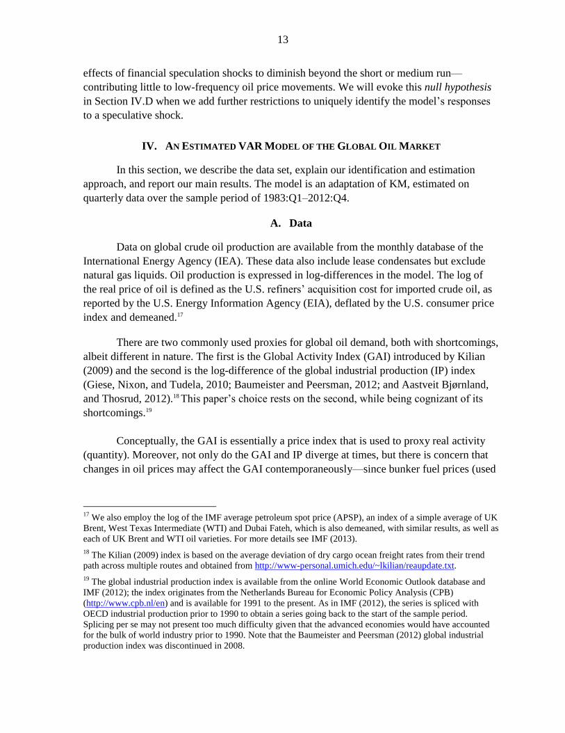
Data on global crude oil production are available from the monthly database of the

International Energy Agency (IEA). These data also include lease condensates but exclude

natural gas liquids. Oil production is expressed in log-differences in the model. The log of

the real price of oil is defined as the U.S. refiners’ acquisition cost for imported crude oil, as

reported by the U.S. Energy Information Agency (EIA), deflated by the U.S. consumer price

index and demeaned.17

There are two commonly used proxies for global oil demand, both with shortcomings,

albeit different in nature. The first is the Global Activity Index (GAI) introduced by Kilian

(2009) and the second is the log-difference of the global industrial production (IP) index

(Giese, Nixon, and Tudela, 2010; Baumeister and Peersman, 2012; and Aastveit Bjørnland,

and Thosrud, 2012).18 This paper’s choice rests on the second, while being cognizant of its

shortcomings.19

Conceptually, the GAI is essentially a price index that is used to proxy real activity

(quantity). Moreover, not only do the GAI and IP diverge at times, but there is concern that

changes in oil prices may affect the GAI contemporaneously—since bunker fuel prices (used

17

We also employ the log of the IMF average petroleum spot price (APSP), an index of a simple average of UK

Brent, West Texas Intermediate (WTI) and Dubai Fateh, which is also demeaned, with similar results, as well as

each of UK Brent and WTI oil varieties. For more details see IMF (2013).

18 The Kilian (2009) index is based on the average deviation of dry cargo ocean freight rates from their trend

path across multiple routes and obtained from http://www-personal.umich.edu/~lkilian/reaupdate.txt.

19 The global industrial production index is available from the online World Economic Outlook database and

IMF (2012); the index originates from the Netherlands Bureau for Economic Policy Analysis (CPB)

(http://www.cpb.nl/en) and is available for 1991 to the present. As in IMF (2012), the series is spliced with

OECD industrial production prior to 1990 to obtain a series going back to the start of the sample period.

Splicing per se may not present too much difficulty given that the advanced economies would have accounted

for the bulk of world industry prior to 1990. Note that the Baumeister and Peersman (2012) global industrial

production index was discontinued in 2008.

14

for cargo freight shipping in the GAI) and the oil price are correlated. 20 However, Baumeister

and Kilian (2013) have compared the forecasting power of the OECD industrial production

index and the GAI for the real oil price and have shown that the GAI outperforms the OECD

IP index. At the same time, Beckers and Beidas-Strom (forthcoming), employ this paper’s IP

index in a reduced-form VAR for forecasting purposes to show that it consistently

outperforms the futures curve, random-walk models and the same VAR when the GAI is

employed, amongst others.21

We use total OECD crude inventories provided by the IEA database as a proxy for

global inventories and hence speculative demand for oil.22,23 We transform the crude

inventories data by taking level changes, since our model is stationary. Preliminary tests

provide no evidence of co-integration between oil production and crude inventories.

Moreover, contrary to the findings of Dvir and Rogoff (2013) for the United States, we find

no evidence of a trend in the rate of crude oil inventory accumulation in recent years.

B. Model Specification

Our setup is a four-variable, four-lags VAR estimated on quarterly data from

1983:Q1 to 2012:Q4. Variables are as follows: , is the log-difference in global crude

oil production (flow oil production above the ground); is the log-difference of the

global industrial production index, which captures flow demand for crude oil; is the

log of the demeaned real price of oil; and is the level change in OECD crude oil

inventories introduced to help identify speculative shocks.24

It may seem that our global oil spot market model is incomplete in that it excludes the

20

See the appendix for more details on: visual differences between the Global Activity Index and Global

Industrial Production Index; visual co-movement between bunker fuels and the oil price; and results of

contemporaneous correlations between the GAI and fuel/oil. 21

Beckers and Beidas-Strom (forthcoming 2013) also add interest rates, spreads, and an exchange rate for the

USD weighted against currencies of major oil consumers; and disaggregate global IP (by emerging and

advanced economies) and oil production and demand by regions (OPEC, North America, and the largest oil

consuming advanced and emerging economies); and add non-commercial futures positions in crude oil as a

ratio of total open interest. 22

The OECD data start in 1983, hence the start of our sample. While data on non-OECD crude oil inventories is

not available, some partial individual country data is available, which seems to indicate a coverage of forward

demand of well-below OECD levels, at about 40 days. See recent issues of the IEA Monthly Oil Report and

Petroleum Intelligence Weekly (available to subscribers). There are also crude inventories held by commodity

trading houses and in transit. The fact that our dataset for crude oil inventories is incomplete will likely show up

in the residual demand shock of the historical decomposition. 23

This is a departure from Kilian and Murphy (2012) and (2013), who use data for total U.S. crude oil

inventories provided by the EIA, scaled by the ratio of OECD petroleum stocks over U.S. petroleum stocks,

also obtained from the EIA. Kilian and Lee (2013) access a global inventories database compiled from

proprietary data from the Energy Intelligence Group (EIG), a private sector company. Despite the complete

dataset, they find the results of KM (2013) largely unaltered. 24

See the appendix for more details on the model description.

15

price of oil futures contracts, which is commonly viewed as an indicator of market

expectations about future oil prices. As mentioned in section III, this is not the case since, as

suggested by Alquist and Kilian (2010) and KM, most of the relevant information is included

in the inventory data. This is also consistent with the fact that the oil futures spread does not

Granger-cause the variables in our model.

C. Estimation Methodology and Identification

The reduced-form VAR model is consistently estimated by least-squares. We initially

partially identify the model using sign restrictions combined with additional empirically

plausible bounds on the magnitude of the short-run oil supply elasticity and on the response

of global demand.25

Initial Specification: Dynamic Sign Restrictions and Elasticities Bounds

Below we summarize the economic intuition behind the imposed sign restriction scheme:

An unexpected flow supply shock is associated with a negative response of oil

production (for at least four quarters), a positive response of the real oil price, and

lower global activity on impact. Hence, a negative oil supply shock shifts the oil

supply curve to the left, lowering the quantity of oil supplied to the market and raising

the real oil price, and therefore lowering global economic activity. We do not restrict

the response of inventories.

A global flow demand shock induces an increase in real activity (for at least four

quarters), shifting the contemporaneous oil demand curve to the right along the oil

supply curve, raising the real oil price and stimulating oil production on impact. We

do not restrict the response of inventories once again.

A speculative demand shock, whatever its motive, embodies a shift in crude oil

inventory demand, and thus is associated with an increase in crude oil inventories and

the real price of oil. The accumulation of inventories requires oil production to

increase and oil consumption (and hence real activity) to decline.

Finally, we impose the cross-restriction that over the long term (defined here to be

20 years), declining oil prices have to be associated with no increase in the level of

inventories.

The model also includes a residual oil demand shock designed to capture

idiosyncratic oil-specific demand shocks driven by reasons that cannot be classified as any

one of the first three structural shocks (such as changes in inventory technology or

preferences, or politically motivated releases of the U.S. Strategic Petroleum Reserve).

25

See the appendix for the procedure used to implement the identification.

16

The admissible models thus take the form—with missing signs denoting that no

restrictions are applied:

That is,

.

Boundary restrictions

In addition to these sign restrictions, following Kilian and Murphy (2012), the model

imposes an upper bound on the impact price elasticity of oil supply so as not to generate

unrealistically large oil supply responses to demand in the short run and restricts the impact

price elasticity of oil demand to be negative and smaller in magnitude than the long-run price

elasticity of oil demand. The latter ranges between 0.1 and 0.6 (IMF, 2011a). The price

elasticity of oil supply and the price response to flow demand with respect to the speculative

demand shock can be expressed as

—price elasticity of oil supply.26

.

Overall, the restrictions imposed narrow the admissible models to about 1,100 from 5 million

candidates.

Admissible Set of Impulse Responses

We now turn to reporting the overall behavior of the estimated models across our

sample by examining 30 randomly selected models from the full set of admissible impulse

response functions (IRFs) (Figure 2).27 As customary in the literature, the shocks are one

standard deviation.

In response to an unexpected negative oil supply shock (Figure 2, top row), there is a

persistent reduction in oil production, up to 5 percent, and in global industrial production,

26

The bound adopted by Kilian and Murphy (2012), 0.0258, seems to be a conservative upper bound and hence

is used in our paper but multiplied by three since we have quarterly data, rather than monthly.

27 See the appendix for the maximum and minimum impulse responses generated by the estimation.

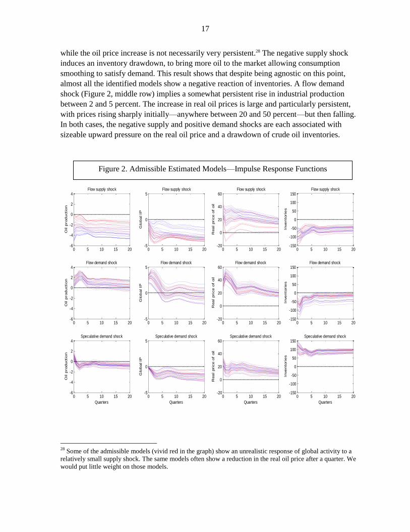
17

while the oil price increase is not necessarily very persistent.28 The negative supply shock

induces an inventory drawdown, to bring more oil to the market allowing consumption

smoothing to satisfy demand. This result shows that despite being agnostic on this point,

almost all the identified models show a negative reaction of inventories. A flow demand

shock (Figure 2, middle row) implies a somewhat persistent rise in industrial production

between 2 and 5 percent. The increase in real oil prices is large and particularly persistent,

with prices rising sharply initially—anywhere between 20 and 50 percent—but then falling.

In both cases, the negative supply and positive demand shocks are each associated with

sizeable upward pressure on the real oil price and a drawdown of crude oil inventories.

28

Some of the admissible models (vivid red in the graph) show an unrealistic response of global activity to a

relatively small supply shock. The same models often show a reduction in the real oil price after a quarter. We

would put little weight on those models.

0 5 10 15 20-6

-4

-2

0

2

4Flow supply shock

Oil p

rod

ucti

on

0 5 10 15 20-5

0

5Flow supply shock

Glo

ba

l IP

0 5 10 15 20-20

0

20

40

60Flow supply shock

Rea

l pri

ce

of

oil

0 5 10 15 20-150

-100

-50

0

50

100

150Flow supply shock

Inve

nto

rie

s

0 5 10 15 20-6

-4

-2

0

2

4Flow demand shock

Oil p

rod

ucti

on

0 5 10 15 20-5

0

5Flow demand shock

Glo

ba

l IP

0 5 10 15 20-20

0

20

40

60Flow demand shock

Rea

l pri

ce

of

oil

0 5 10 15 20-150

-100

-50

0

50

100

150Flow demand shock

Inve

nto

rie

s

0 5 10 15 20-6

-4

-2

0

2

4Speculative demand shock

Oil p

rod

ucti

on

Quarters

0 5 10 15 20-5

0

5Speculative demand shock

Glo

ba

l IP

Quarters

0 5 10 15 20-20

0

20

40

60Speculative demand shock

Rea

l pri

ce

of

oil

Quarters

0 5 10 15 20-150

-100

-50

0

50

100

150Speculative demand shock

Inve

nto

rie

s

Quarters

Figure 2. Admissible Estimated Models—Impulse Response Functions

18

Finally, the speculative demand shock: demand for physical inventories temporarily

pushes up the spot real oil price by anywhere between 10 and 35 percent (Figure 2, bottom

row), but then the price gradually declines. Interestingly, oil production—restricted to rise at

impact—eventually declines under all the admissible models, bringing down also global

industrial production in a manner similar to the flow supply shock.

D. When Does Speculative Demand Matter?

Under the null hypothesis that anomalies in futures markets are temporary, the

expectation is that financial speculation can increase the short-run oil price volatility (through

shifts in the demand for oil inventories), but it should contribute little to low-frequency

fluctuations. To shed some light on the role of financial speculation shocks, we use two

strategies; each one imposes an additional restriction on the set of admissible models:

i. Interpreting strictly the null hypothesis, we select the model that has the lowest

contribution of the speculative demand shock to the real oil price forecast error

variance (MFEV, for short) at 20 years (intended to indicate the long run), while

being agnostic about the short-term effects.

Given that this restriction may look too conservative, effectively “minimizing” the oil

price volatility, we also use a less stringent interpretation of our null hypothesis:

ii. We select the model that maximizes the difference between the short- and long-run

oil price reaction to a speculative shock—in other words, the impulse response

function with the largest slope (the Max Ratio, for short).

With these two restrictions, we will be able to determine the range of impact from

speculation, whereby mispricing in the futures market has an estimated minimum and

maximum in terms of its effect on short-run oil prices—which is manifest in shifts in

inventory demand. Our proposed additional restrictions outlined above rest on economic

theory (rather than statistical methods). In other words, we do not compute cumbersome

posterior distributions of outcomes. Nor do we adopt the simpler approach of picking the

median impulse response function from the set of admissible models since each model/IRF

would be equally consistent with the observed data and underlying restrictions (as shown in

Fry and Pagan, 2011).

Our results are shown in Figure 3. The first results shown are the MFEV (solid black

lines). With this restriction, however, other shocks such as risk premium shocks and news

shocks related to events that are expected to be temporary are also captured. Even so, the

total contribution of this type of speculative shock is very modest. Indeed, while a temporary

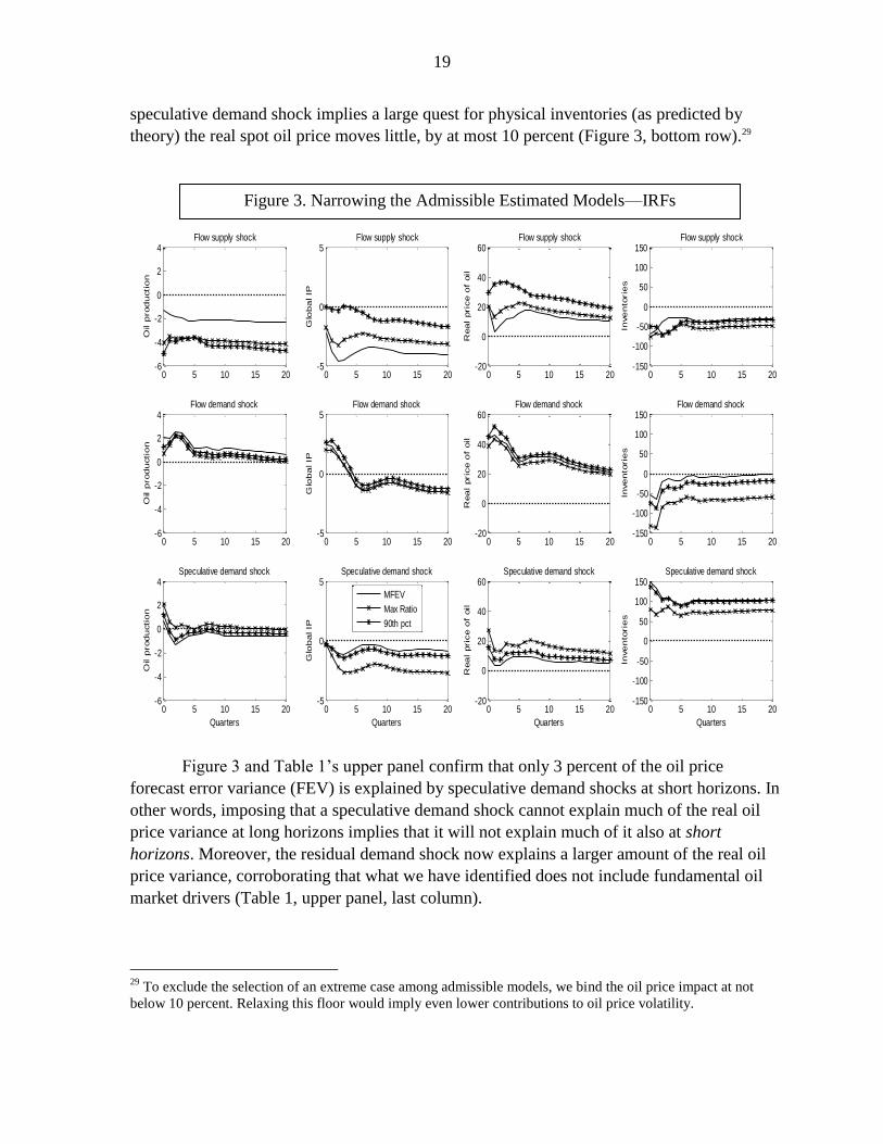
19

speculative demand shock implies a large quest for physical inventories (as predicted by

theory) the real spot oil price moves little, by at most 10 percent (Figure 3, bottom row).29

Figure 3 and Table 1’s upper panel confirm that only 3 percent of the oil price

forecast error variance (FEV) is explained by speculative demand shocks at short horizons. In

other words, imposing that a speculative demand shock cannot explain much of the real oil

price variance at long horizons implies that it will not explain much of it also at short

horizons. Moreover, the residual demand shock now explains a larger amount of the real oil

price variance, corroborating that what we have identified does not include fundamental oil

market drivers (Table 1, upper panel, last column).

29

To exclude the selection of an extreme case among admissible models, we bind the oil price impact at not

below 10 percent. Relaxing this floor would imply even lower contributions to oil price volatility.

0 5 10 15 20-6

-4

-2

0

2

4Flow supply shock

Oil p

rod

ucti

on

0 5 10 15 20-5

0

5Flow supply shock

Glo

ba

l IP

0 5 10 15 20-20

0

20

40

60Flow supply shock

Rea

l pric

e o

f oil

0 5 10 15 20-150

-100

-50

0

50

100

150Flow supply shock

Inve

nto

rie

s

0 5 10 15 20-6

-4

-2

0

2

4Flow demand shock

Oil p

rod

ucti

on

0 5 10 15 20-5

0

5Flow demand shock

Glo

ba

l IP

0 5 10 15 20-20

0

20

40

60Flow demand shock

Rea

l pric

e o

f oil

0 5 10 15 20-150

-100

-50

0

50

100

150Flow demand shock

Inve

nto

rie

s

0 5 10 15 20-6

-4

-2

0

2

4Speculative demand shock

Oil p

rod

ucti

on

Quarters

0 5 10 15 20-5

0

5Speculative demand shock

Glo

ba

l IP

Quarters

0 5 10 15 20-20

0

20

40

60Speculative demand shock

Rea

l pric

e o

f oil

Quarters

0 5 10 15 20-150

-100

-50

0

50

100

150Speculative demand shock

Inve

nto

rie

s

Quarters

MFEV

Max Ratio

90th pct

Figure 3. Narrowing the Admissible Estimated Models—IRFs

20

Flow oil supply shock Flow demand shock Speculative demand shock Residual shock

Horizon

13 58 3 27

8 49 2 41

Horizon

13 45 22 21

14 41 13 31

Horizon

21 44 19 17

19 35 21 25

Table 1. Real Oil Price Variance Decomposition (1984:1-2012:12)

MFEV model

Average of all Admissiable models

1 quarter

20 years

1 quarter

20 years

Max Ratio Model

1 quarter

20 years

Now to give temporary speculative demand shocks the best chance of affecting the

short-run oil price through a shift in demand for inventories (i.e., to obtain a plausible

maximum), we choose the IRF with the steepest slope after impact (the Max Ratio).

The response of the oil price under the Max Ratio restriction is almost three times

greater than that under the MFEV restriction (Figure 3, bottom row, third column). The

variance contribution of the speculative shock in the short term substantially increases to 22

percent, while the residual demand shock explains less of the variance (Figure 3 and Table 1,

lower panel). The contribution at longer horizons, however, at 13 percent, becomes no longer

negligible! This number is actually not far from the median contribution across all admissible

models.30 In other words, it no longer looks like the effect of short-run speculative demand;

rather it seems now to be “contaminated” by reactions of market participants to “news

shocks.”

Overall, our findings suggest that the impact response of the oil price to speculative

demand shocks driven by temporary motives in explaining the short-run real oil price

volatility lie between 10 to 35 percent—second to those of flow demand (between 40 to

45 percent) but conceivably larger than that of flow supply (at 20 percent). This means that

news on temporary supply disruptions or movements in risk premiums or perhaps financial

speculation have played a nonnegligible role in moving oil prices in the short run. Moreover,

those shocks explain a large part of inventory volatility, confirming the helpful role

inventories play in stabilizing oil prices through increasing effective supply (Figure 3).

Finally, we have shown in section III that news on future shifts in oil demand and

production schedules can show up as speculative demand shocks. However, in this case there

30

Within the admissible set of identified models, the maximum contribution to the oil price forecast error

variance is 47 percent at the one-quarter horizon and 35 percent at the 20 year horizon.

21

is no reason to believe that such speculative demand shocks would have no long-run effect

on prices. In this case, we find the effects on prices could be substantial. Figure 3 shows the

IRFs of the 90th

percentile (on the oil price impact). This type of shock has the smallest

impact on inventories but the highest on prices, showing that in general news shocks

contribute substantially to short-run oil price volatility—pushing the price up (or down) by

35 percent. Moreover, since oil production eventually declines (even if constrained to rise on

impact), it suggests that most of those news shocks are related in some way to expectation

shifts in future production possibilities.

Historical decomposition

The historical decomposition focuses on the cumulative effects at each point in time

of the flow supply shock, flow demand shock, speculative demand shock, and residual

demand shock. Unlike KM, whose choice of historical decomposition relied on statistical

methods,31 our contribution is that we rest on economic theory—which has allowed us to

build a model (without need for data on oil futures) wherein shocks to above-the-ground

holdings of oil inventories, that is, speculative demand shocks, can cause temporary

mispricing of oil futures and spill over to short-run spot prices.

Figure 4 shows how the demeaned real oil price would have evolved if all structural

shocks barring the one in question had been turned off. So, for example, a bar that is

increasing over time means that the shock the bar refers to is exerting upward pressure on the

real oil price. The left panel displays the results from the restriction that minimized the long

run oil price forecast error variance (MFEV). It highlights the dominance of flow demand

shocks across the full sample even though speculative demand shocks played a role in the

recent period. Interestingly, the run-up of oil prices during 2003–08 can be seen to be driven

initially and solely by flow demand, but importantly since 2005 onward, flow demand is

joined by speculative demand shocks—this occurring at the exact time when indexed-fund

investors (hedge and pension funds) entered commodity markets, along with commodity

trading houses which began to hedge (increasing) physical assets with financial instruments.

Following the global financial crisis (i.e. during 2011–12), the 2005 drivers re-emerge and oil

supply takes a more subdued role.

The right panel displays the results of the restriction that maximizes the ratio of the

short-run oil price forecast error variance to that of the long run (Max Ratio). In this setting,

flow demand loses some importance but, interestingly, speculative demand (due to the

forward-looking behavior of oil market players) and the residual demand shock play the

dominant role. In addition, oil supply picks up power.

31

KM uniquely identify speculative demand with Bayesian priors and select the mode of the distribution. This

choice of identification has important implications for the estimated impact of speculative demand shocks on

the real oil price (or lack thereof).

22

Model A—Identification minimizes the oil price forecast

error variance due to speculation in the Long Run (MFEV)

Model B—Identification maximizes the oil price forecast

error variance (FEV)/ Long Run FEV (Max Ratio)

Perhaps an even simpler approach to gauging the relative role of shocks is to examine

their absolute contribution over time, to abstract from negative and positive movements.

Figure 5 confirms that when using the MFEV restriction (left panel), flow demand is most

prominent across the sample, with some downplay of the relative size of supply disruptions,

(e.g., the 1990 Iraq invasion of Kuwait). On the other hand, when the Max Ratio restriction is

0

10

20

30

40

50

60

70

80

90

100

-2

-1

-1

0

1

1

2

85Q3 88Q3 91Q3 94Q3 97Q3 00Q3 03Q3 06Q3 09Q3 12Q3

Contr

ibution o

f shocks

Model A--Identification minimizes the oil price forecast error variance due to speculation in LR

Speculative demand shock

Residual shock

Flow demand shock

Flow oil supply shock

Real oil price (in US dollars)

0

10

20

30

40

50

60

70

80

90

100

-2

-1

-1

0

1

1

2

85Q3 88Q3 91Q3 94Q3 97Q3 00Q3 03Q3 06Q3 09Q3 12Q3

Contr

ibution o

f shocks

Model B--Identification maximizes the oil price forecast error variance (FEV) / FEV in LR to ratio

Speculative demand shock

Residual demand shock

Flow demand shock

Flow oil supply shock

Real oil price (in US dollars)

0%

10%

20%

30%

40%

50%

60%

70%

80%

90%

100%

1985Q1 1988Q1 1991Q1 1994Q1 1997Q1 2000Q1 2003Q1 2006Q1 2009Q1 2012Q1

Residual demand contribution Speculative demand contribution

Flow demand contribution Flow supply contribution

0%

10%

20%

30%

40%

50%

60%

70%

80%

90%

100%

1985Q1 1988Q1 1991Q1 1994Q1 1997Q1 2000Q1 2003Q1 2006Q1 2009Q1 2012Q1

Residual demand contribution Speculative demand contribution

Flow demand contribution Flow supply contribution

Figure 4. Historical Decomposition of the Drivers of the Real Oil Price

Figure 5. Absolute Drivers of the Real Oil Price

23

used (right panel), speculative demand shocks induce inventory demand shifts. Thus, our

results confirm that the identification and set of restrcitions matter appreciably when deciding

on the relative importance of various shocks on the real oil price. Overall, we conclude that

all four types of shocks (flow demand, speculative demand, supply and residual demand)

have influenced the real oil price.

V. CONCLUSION

We have attempted in this paper to explore the short-term effects of speculative oil

demand. In the Kilian and Murphy (2013) SVAR framework, one cannot distinguish between

speculative demand shocks driven by news about fundamentals and those driven by noise

trading. While we use this framework, we have proposed additional restrictions to estimate a

range for the short-term impact of speculative demand shocks, regardless of their motive

(destabilizing or not). These additional restrictions are on the contribution of speculative

demand shocks to the long-run oil price forecast error variance—i.e., by imposing

restrictions on the time horizon during which noise trading and other factors affect oil

markets. They have allowed us to estimate the range (a minimum and a maximum) of the real

oil price response to speculative demand shocks.

We have imposed these additional restrictions using economic theory: specifically

that arbitrage by fundamental traders should ensure that oil prices are in line with

fundamentals in the long run. With this in mind, our null hypothesis is that only oil market

fundamentals (or news about them) can induce low-frequency movements in oil prices.

Under the null hypothesis, mispricing in the futures market (i.e., noise trading by financial

speculators) is a temporary anomaly that does not contribute to low-frequency price

movements. Therefore it is possible to narrow its contribution to short-run oil price volatility

by restricting our attention to the admissible model that minimizes the oil price forecast error

variance’s contribution of speculative shocks at long horizons (e.g., 20 years).

We have shown that news shocks on oil market fundamentals, mispricing in the oil

futures market, and global real interest rate shocks can manifest themselves as speculative

demand shocks (shifts in inventory demand) under the Kilian and Murphy (2013)

identification strategy. Hence, we have proposed a novel manner to put a plausible bound on

the contribution of financial speculation to short-term oil price volatility (which lies between

3 and 22 percent). We find the impact response of the oil price to a speculative shock to be

smaller (between 10 to 35 percent) than that of a shock to flow demand (between 40 to 45

percent) but conceivably larger than that of a shock to flow supply (at 20 percent).

We find that the type of speculative demand identified through our restrictions

matters for the historical decomposition in terms of the factors that have contributed to oil

price fluctuations. Specifically, we find that when speculative demand is confined to be short

in duration, with small long-run effects on the real oil price, the run-up in oil prices during

2003–08 can be attributed initially to flow oil demand shocks. Speculative demand shocks

24

also contributed but only marginally after 2005—with the same drivers re-emerging again

during 2011–12. However, when we allow speculative demand shocks to have larger effects

in the short and long run (i.e. using our maximum), flow oil demand shocks have contributed

less.

25

REFERENCES

Aastveit, K. A., H. C. Bjørnland, L. A. Thorsrud, 2012, “What Drives Oil Prices? Emerging

versus Developed Economies,” mimeo, Norge Bank.

Alquist, R., and L. Kilian, 2010, "What do We Learn from the Price of Crude Oil Futures?"

Journal of Applied Econometrics, John Wiley & Sons, Ltd., Vol. 25(4), pp. 539–573.

Backus, D. K., and M. J. Crucini, 2000, “Oil Prices and the Terms of Trade,” Journal of

International Economics, Vol. 50 (February), pp. 185–213.

Baumeister, C., and L. Kilian, 2013, “What Central Bankers Need to Know about

Forecasting Oil Prices,” forthcoming: International Economic Review.

Baumeister, C., and G. Peersman, 2012, “The Role of Time-Varying Price Elasticities in

Accounting for Volatility Changes in the Crude Oil Market,” Journal of Applied

Econometrics.

Beckers, B., and S. Beidas-Strom, forthcoming, “Forecasting Nominal Prices of International

Oil Benchmarks—An Ex Post Statistical Assessment” IMF Working Paper.

Brennan, M. J., 1958, “The Supply of Storage,” American Economic Review, 47, pp. 50–72.

Büyükşahin, B., and M. A. Robe, 2012, “Speculators, Commodities and Cross-Market

Linkages,” available at SSRN: http://ssrn.com/abstract=1707103 or

http://dx.doi.org/10.2139/ssrn.1707103.

Dvir, E., and K. Rogoff, 2013, “Evidence and Speculation in Oil Markets: Theory and

Evidence,” from Understanding Commodity Market Fluctuations, IMF-Oxford

Conference, Washington DC, March, 2013, and forthcoming in the Journal of

International Money and Finance.

Fama, E. F., 1998, “Market Efficiency, Long-Term Returns, and Behavioral Finance,”

Journal of Financial Economics, 49 (1998) 283D306.

Fattouh, B., L. Kilian, and R. Mahadeva, 2012, “The Role of Speculation in Oil Markets:

What Have we Learned so Far?” Forthcoming: Energy Journal.

Fry, R., and A. Pagan, 2011, “Sign Restrictions in Structural Vector Autoregressions: A

Critical Review,” Journal of Economic Literature, American Economic Association,

vol. 49(4), pages 938-60, December.

Giese, J., D. Nixon, and M. Tudela, 2010, “How Well Can We Explain Movements in the Oil

Price?” Bank of England Commodity Watch: Technical Briefing.

26

Gromb, D., and D. Vayanos, 2010, “Limits of Arbitrage: The State of the Theory,” NBER

Working Paper No. 15821.

Hamilton J. D., 2009, “Causes and Consequences of the Oil Shock of 2007–08,” Brookings

Papers on Economic Activity (Spring), pp. 215–261.

International Monetary Fund, 2011a, Chapter 3: Oil Scarcity, Growth, and Global

Imbalances, World Economic Outlook (April).

________, 2011b, Box 1.4, “Financial Investment, Speculation, and Commodity Prices,”

World Economic Outlook (October).

________, 2012, Chapter 2, “Commodity Price Swings and Commodity Exporters,” World

Economic Outlook (April).

________, 2013, Box 1.SF.2, “Oil Price Drivers and the Narrowing WTI-Brent Spread,”

World Economic Outlook (October).

Jaimovich, Nir, and Sergio Rebelo, 2009, “Can News about the Future Drive the Business

Cycle?” American Economic Review, 99(4), 1097–1118.

Juvenal, L. and I. Petrella, 2011, “Speculation in the Oil Market,” Working Papers 2011–027,

Federal Reserve Bank of St. Louis.

Kaldor, N., 1939, “Speculation and Economic Stability,” Review of Economic Studies 7:1-27.

Kilian, L., 2009, “Not All Oil Price Shocks Are Alike: Disentangling Demand and Supply

Shocks in the Crude Oil Market,” American Economic Review, 99(3): 1053–69.

Kilian, L., and T. Lee, 2013, “Quantifying the Speculative Component in the Real Price of

Oil: The Role of Global Oil Inventories,” from Understanding Commodity Market

Fluctuations, IMF-Oxford Conference, Washington D.C., March, 2013, and

forthcoming in the Journal of International Money and Finance.

Kilian, L., and D. Murphy, 2012, “Why Agnostic Sign-Restrictions Are Not Enough:

Understanding the Dynamics of the Oil Market VAR Models,” Journal of European

Economic Association, October 2012 10(5):1116–1188.

_________, 2013, “The Role of Inventories and Speculative Trading in the Global Market

for Crude Oil,” Journal of Applied Econometrics, forthcoming.

Kilian, L., and C. Vega, 2011, "Do Energy Prices Respond to U.S. Macroeconomic News? A

Test of the Hypothesis of Predetermined Energy Prices," The Review of Economics

and Statistics, MIT Press, Vol. 93(2), pp. 660–671.

27

Knittel, C. R., and R. S. Pindyck, 2013, “The Simple Economics of Commodity Price

Speculation,” NBER Working Paper Series, No. 18951.

Liu, P., and K. Tang, 2010, “Bubbles in the Commodity Asset Class: Detection and

Sources,” SSRN eLibrary (SSRN).

Masters, M. W., 2008, Testimony before the Committee on Homeland Security and

Governmental Affairs United States Senate, “The 2008 Commodities Bubble:

Assessing the Damage to the United States and Its Citizens,” Special Report:

http://www.hsgac.senate.gov//imo/media/doc/052008Masters.pdf?attempt=2

Nakov, A. and A. Pescatori, 2010, "Oil and the Great Moderation," Economic Journal, Royal

Economic Society, vol. 120(543), pp. 131–156, 03.

Scheinkman, J. A., and J. Schechtman, 1983, “A Simple Competitive Model with Production

and Storage,” Review of Economic Studies, 50, 427–441.

Singleton, K. J., 2011, “Investor Flows and the 2008 Boom/Bust in Oil Prices,” Graduate

School of Business, Stanford University, mimeo.

Tang, K., and W. Xiong, 2010, “Index Investment and Financialization of Commodities,”

NBER Working Papers, National Bureau of Economic Research, Inc.

Telser, L. G., 1958, "Futures Trading and the Storage of Cotton and Wheat,” Journal of

Political Economy, 66, 233–255.

Working, H., 1934, “Theory of Inverse Carrying Charge in Futures Markets,” Journal of

Farm Economics, 30, 1–28.

28

APPENDIX

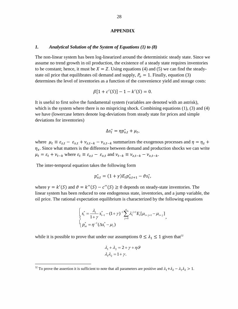
1. Analytical Solution of the System of Equations (1) to (8)

The non-linear system has been log-linearized around the deterministic steady state. Since we

assume no trend growth in oil production, the existence of a steady state requires inventories

to be constant; hence, it must be . Using equations (4) and (5) we can find the steady-

state oil price that equilibrates oil demand and supply, . Finally, equation (3)

determines the level of inventories as a function of the convenience yield and storage costs:

.

It is useful to first solve the fundamental system (variables are denoted with an astrisk),

which is the system where there is no mispricing shock. Combining equations (1), (3) and (4)

we have (lowercase letters denote log-deviations from steady state for prices and simple

deviations for inventories)

,

where summarizes the exogenous processes and

. Since what matters is the difference between demand and production shocks we can write

where and .

The inter-temporal equation takes the following form

where and depends on steady-state inventories. The

linear system has been reduced to one endogenous state, inventories, and a jump variable, the

oil price. The rational expectation equilibrium is characterized by the following equations

* * 1 111 1 1

0

* 1 *

(1 ) [ ]1

( )

j

t t t t j t j

j

ot t t

s s E

p s

,

while it is possible to prove that under our assumptions given that32

1 2

1 2

2

1 .

32

To prove the assertion it is sufficient to note that all parameters are positive and .

29

Finally, the log-linear futures price is simply determined by log-linearizing equation (7):

.

We now turn to the determination of the actual system where futures prices can deviate from

fundamentals, which can be written as

, 1

*

, 1 , 1

(1 )

t ot t

ot t t t

t t t t t

s p

p f s

f f

.

Since the steady state is the same as in the fundamental system and, in absence of shocks, the

two systems are by construction the same, it is possible to describe the non-fundamental

system as deviations from the fundamental system (variables are denoted with a tilde: e.g., )

(1 )

t ot

ot t t

s p

p s

.

The system has a simple solution

1

1

1 1

1

1 1

t tt

tot t

ss

sp

.

2. Differences between the Global Activity Index and Global Industrial Production

GAI and IP diverge at times, including at times of structural change in the shipping sector.

For example, this has been the case in the period since 2011, when freight costs collapsed

with the onset of large economies of scale in shipping—i.e., when Chinamax and cape

vessels, triple or double the size of Panamax, came on stream (figure below, grey dashed

circles).

30

There is also concern that GAI and oil prices move contemporaneously—since the GAI

incorporates bunker fuel prices (used for cargo freight shipping). This appears to be the case

for the most commonly traded bunker fuel varieties shown along the major dry bulk shipping

routes, indicating that the real oil price has a contemporaneous effect on the GAI at monthly

and quarterly frequency.

We find the contemporaneous correlation between GAI and Brent or WTI to be mildly

positive (about 0.3), while the contemporaneous correlation between GAI and the bunker fuel

(figure above) is stronger: about 0.4.

-100

-80

-60

-40

-20

0

20

40

60

80

100

-0.10

-0.08

-0.06

-0.04

-0.02

0.00

0.02

0.04

0.06

0.08

0.10

73 75 77 79 81 83 85 87 89 91 93 95 97 99 01 03 05 07 09 11

First Difference of log IP Index

Real Global Activity Index (Baltic Dry Bulk) (RHS)

Economic booms missed by the

GAI

Boom in GAI due to

shipping shortages not present in IP

Major slump in GAI due to dry bulk shipping vessel

oversupply

GAI co-moves sharply with fall in

oil prices

Sources: IMF WEO database; Kilian's webpage: http://www-personal.umich.edu/~lkilian/reaupdate.txt.; and authors' estimates.

Global Activity Index vs. Global Industrial Production Index

31

3. Standard VAR(4) Model Representation

Consider a 4-dimensional vector , l lags, and matrices of coefficients and such that

As explained by Hamilton (1994), since the structural disturbances are related to the VAR

innovations, , we can represent them by:

If the structural VAR representation has the following form:

,

where denotes the (4 × 1) vector of serially and mutually uncorrelated structural

innovations, is a (4 × 1) vector of constants, and 0, …, l, denotes the impact or

coefficient matrices at the l-th lag where the demand and supply elasticity are contained.

Then to have the orthogonalised innovations to coincide with the true structural disturbances

we must have:

0

20

40

60

80

100

120

140

160

0

100

200

300

400

500

600

700

800

900

2006 2007 2008 2009 2010 2011 2012 2013

US

D/B

arr

el

US

D/M

etr

ic T

onne

Selected Bunker Fuel and Oil Price Co-movements

Rotterdam180 Rotterdam360 Singapore180 Singapore380

Houston180 Houston380 Brent Oil (RHS) WTI (RHS)

Sources: Bloomberg, L.P.; and IMF, Primary Commodity Price System.

32

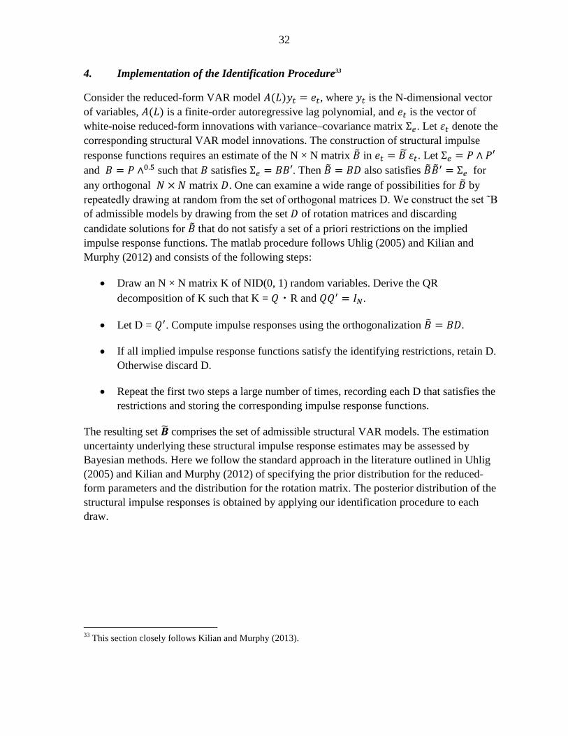
4. Implementation of the Identification Procedure33

Consider the reduced-form VAR model , where is the N-dimensional vector

of variables, is a finite-order autoregressive lag polynomial, and is the vector of

white-noise reduced-form innovations with variance–covariance matrix . Let denote the

corresponding structural VAR model innovations. The construction of structural impulse

response functions requires an estimate of the N × N matrix in . Let

and such that satisfies . Then also satisfies for

any orthogonal matrix . One can examine a wide range of possibilities for by

repeatedly drawing at random from the set of orthogonal matrices D. We construct the set ˜B

of admissible models by drawing from the set of rotation matrices and discarding

candidate solutions for that do not satisfy a set of a priori restrictions on the implied

impulse response functions. The matlab procedure follows Uhlig (2005) and Kilian and

Murphy (2012) and consists of the following steps:

Draw an N × N matrix K of NID(0, 1) random variables. Derive the QR

decomposition of K such that K = ・R and .

Let D = . Compute impulse responses using the orthogonalization

If all implied impulse response functions satisfy the identifying restrictions, retain D.

Otherwise discard D.

Repeat the first two steps a large number of times, recording each D that satisfies the

restrictions and storing the corresponding impulse response functions.

The resulting set comprises the set of admissible structural VAR models. The estimation

uncertainty underlying these structural impulse response estimates may be assessed by

Bayesian methods. Here we follow the standard approach in the literature outlined in Uhlig

(2005) and Kilian and Murphy (2012) of specifying the prior distribution for the reduced-

form parameters and the distribution for the rotation matrix. The posterior distribution of the

structural impulse responses is obtained by applying our identification procedure to each

draw.

33

This section closely follows Kilian and Murphy (2013).

33

5. Maximum and Minimum Impulse Responses Generated by the Estimation,

Quarterly Frequency

0 5 10 15 20-6

-4

-2

0

2

4Flow supply shock

Oil p

rod

ucti

on

0 5 10 15 20-6

-4

-2

0

2

4

6Flow supply shock

Glo

ba

l IP

0 5 10 15 20-20

0

20

40

60Flow supply shock

Rea

l pric

e o

f oil

0 5 10 15 20-200

-100

0

100

200Flow supply shock

Inve

nto

rie

s

0 5 10 15 20-6

-4

-2

0

2

4Flow demand shock

Oil p

rod

ucti

on

0 5 10 15 20-6

-4

-2

0

2

4

6Flow demand shock

Glo

ba

l IP

0 5 10 15 20-20

0

20

40

60Flow demand shock

Rea

l pric

e o

f oil

0 5 10 15 20-200

-100

0

100

200Flow demand shock

Inve

nto

rie

s

0 5 10 15 20-6

-4

-2

0

2

4Speculative demand shock

Oil p

rod

ucti

on

Quarters

0 5 10 15 20-6

-4

-2

0

2

4

6Speculative demand shock

Glo

ba

l IP

Quarters

0 5 10 15 20-20

0

20

40

60Speculative demand shock

Rea

l pric

e o

f oil

Quarters

0 5 10 15 20-200

-100

0

100

200Speculative demand shock

Inve

nto

rie

s

Quarters