The Price of Oil Risk

Steven D. Baker,∗ Bryan R. Routledge,†

[February 10, 2017]

Abstract We solve a Pareto risk-sharing problem for two agents with heterogeneous re-cursive utility over two goods: oil, and a general consumption good. Using the optimalconsumption allocation, we derive a pricing kernel and the price of oil and related futurescontracts. This gives us insight into the dynamics of prices and risk premia. We computeportfolios that implement the optimal consumption policies, and demonstrate that largeand variable open interest is a property of optimal risk-sharing. A numerical example ofour model shows that rising open interest and falling oil risk premium are an outcome ofthe dynamic properties of the optimal risk sharing solution.

∗ McIntire School of Commerce, University of Virginia; sdb7e@virginia.edu.† Tepper School of Business, Carnegie Mellon University; routledge@cmu.edu.

1 Introduction

The spot price of crude oil, and commodities in general, experienced a dramatic price

increase in the summer of 2008. For oil, the spot price peaked in early July 2008 at $145.31

per barrel (see Figure 1). In real-terms, this price spike exceeded both of the OPEC price

shocks of 1970’s and has lasted much longer than the price spike at the time of the Iraq

invasion of Kuwait in the summer of 1990. The run-up to the July 2008 price of oil begins

around 2004. Buyuksahin, Haigh, Harris, Overdahl, and Robe (2011) and Hamilton and

Wu (2014) identify a structural change in the behavior of oil prices around 2004. This 2004

to 2008 time period also coincides with a large increase in trading activity in commodities

by hedge funds and other financial firms, as well as a growing popularity of commodity

index funds (see, e.g., CFTC (2008)). In fact, there is much in the popular press that

laid the blame for higher commodity prices, food in particular, on the “financialization”

of commodities.1 Others suggest that since these new traders in futures do not end up

consuming any of the spot commodity, the trading can have little (if any) effect on spot

prices.2 Resolving this debate requires modeling the equilibrium relationship between spot

and futures prices. It also requires a clearer understanding of hedging and speculation.

To achieve this, we look directly at the risk-sharing Pareto problem in an economy with

heterogenous agents and multiple goods, and solve for equilibrium risk premia.

Our intuition about the use and pricing of commodity futures contracts is often expressed

with hedgers and speculators. This dates back to Keynes (1936) and his discussion of

“normal backwardation” in commodity markets. The term backwardation is used in two

closely related contexts. Often it is used to refer to a negatively sloped futures curve where,

e.g., the one-year futures price is below the current spot price. Keynes’ use of the term

1See for example “The food bubble:How Wall Street starved millions and got away with it” by FrederickKaufman, Harpers July 2010 http://harpers.org/archive/2010/07/0083022

2The clearest argument along this lines is by James Hamiltonhttp://www.econbrowser.com/archives/2011/08/fundamentals sp.html. See also Hamilton (2009) andWright (2011)

“normal backwardation” (or “natural”) refers to the situation where the current one-year

futures price is below the expected spot price in one-year. This you will recognize as a risk

premium for bearing the commodity price risk. This relation is “normal” if there are more

hedgers than there are speculators. Speculators earn the risk premium, and hedgers benefit

from off-loading the commodity price risk. But there is no reason to assume that hedgers are

only on one side of the market. Both oil producers (Exxon) and oil consumers (Southwest

Air) might hedge oil. In oil markets in the 2004 to 2008 period, there was a large increase on

the long-side by speculators suggesting the net “commercial” or hedging demand was on the

short side. This is documented in Buyuksahin, Haigh, Harris, Overdahl, and Robe (2011),

who use proprietary data from the CFTC that identifies individual traders. However, if

we are interested in risk premia in equilibrium we need to look past the corporate form of

who is trading. We own a portfolio that includes Exxon, Southwest Air, and a commodity

hedge fund; we consume goods that, to varying degrees, depend on oil. Are we hedgers or

speculators?

Equilibrium risk premia depend on preferences, endowments, technologies, and financial

markets. In this model we focus on complete and frictionless financial markets. We leave

aside production, and consider an endowment economy with two goods. One good we cali-

brate to capture the salient properties of oil; the other we think of as a composite good akin

to consumption in the macro data. We consider two agents with heterogenous preferences

over the two goods, as well as with different time and risk aggregators (using Epstein and

Zin (1989) preferences). Preference heterogeneity is a natural explanation for the portfolio

heterogeneity we see in commodity markets. Here we start with complete and frictionless

markets, focus on “perfect” risk sharing, and solve for the Pareto optimal consumption

allocations. From this solution, we can infer the “representative agent” marginal rates of

substitution, and calculate asset prices and the implied risk premiums.

To see how heterogeneity plays a role, consider an agent who weighs two severe risks: a

recession caused by an oil crisis, and a recession with another root cause – say a financial

2

crisis. Both scenarios are high marginal-rate-of-substitution states. However, in the oil-

lead recession, the price of oil is high. In the financial-crisis-lead recession the oil price is

low. Which is worse? The answer, which depends on preferences, determines the agent’s

attitude towards a short-dated crude oil futures contract, and ultimately determines the

risk premium for a long position in oil. In our numerical example, in Section 4, we have

two agents who rank these scenarios differently. The risk premium on oil depends on

the relative wealth of the two agents. Each agent holds a Pareto-optimal portfolio, but

realized returns may increase the wealth of one agent versus the other. So the longer

horizon risk premiums and their dynamics over time depend on the evolution of the wealth

shares. Because they occur endogenously, changes in the wealth distribution also provide

an alternative (or complementary) explanation for persistent changes in oil markets that

does not rely upon exogenously imposed structural breaks, such as permanent alterations

to the consumption growth process, or changing access to financial markets.

Models of commodity futures typically study either active trade and risk sharing, or

cross-market equilibrium price dynamics, but not both. For example, work in the spirit of

the normal backwardation theory of Keynes and Hicks, such as Hirshleifer (1988) or more re-

cently Baker (2015), allows for hedging using commodity futures, but assumes that revenue

streams are generally non-marketable: agents are either commodity producers or commod-

ity consumers, by virtue of their endowments. By contrast other studies situate commodity

futures in complete financial markets, but consider the dual problems of either a represen-

tative producer (as in Kogan, Livdan, and Yaron (2009)) or a representative household (as

in Ready (2014)), and do not explicitly model trade in futures. Hitzemann (2015) studies

a general equilibrium model with a representative household and a firm that produces and

stores oil, but also without active trade in futures. An exception is Hirshleifer (1990), in

which households receive heterogeneous endowment streams of two goods, and optimally

hedge by trading futures. The elegant theoretical setting, without preference heterogeneity

or intertemporal consumption, is sufficient to demonstrate that futures risk premia are not

3

generally a function of hedging pressure. However these simplifying assumptions render

study of joint spot price and futures open interest dynamics impossible, and the lack of

preference heterogeneity limits the impact of equilibrium wealth dynamics on commodity

prices and risk premia. To overcome this limitation we build on many papers that look

at risk sharing and models with heterogenous agents. We are most closely building on

Backus, Routledge, and Zin (2009) and (2008), with a model structure similar to Colacito

and Croce (2014), but with fewer restrictions on preference parameters. Foundational work

in risk sharing with recursive preferences includes Lucas and Stokey (1984), Kan (1995),

and Anderson (2005).

The bulk of our paper explores a numerical example of our model. The example demon-

strates how dynamic risk sharing between agents with different preferences generates wide

variation in prices, risk premia, and open interest over time. This frictionless Pareto bench-

mark sheds some light on why empirical studies have reached somewhat nuanced conclusions

regarding the connection between futures open interest, spot prices, and financial asset re-

turns. For example Hong and Yogo (2012) find that futures open interest is a good predictor

of commodity and bond returns. A series of papers, including Stoll and Whaley (2010),

Buyuksahin, Haigh, Harris, Overdahl, and Robe (2011), Hamilton and Wu (2014), and

Singleton (2014), discuss the “financialization” of commodity futures markets documented

since around 2004, illustrated by an increase in the number of contracts traded by com-

modity index funds specifically. Stoll and Whaley (2010) find that lagged futures returns

drive out the predictive power of commodity index flows, whereas Singleton (2014) finds the

flows have predictive power after controlling for lagged returns and open interest generally.

As summarized in Irwin and Sanders (2011), evidence on causal linkages between positions

and futures return moments is mixed. Kilian and Murphy (2014) argue that global demand

shocks rather than speculative futures trade explained the 2003-2008 oil price surge. Fi-

nancial trade and consumer demand are impossible to disentangle in our complete markets

equilibrium setting, because the wealth dynamics that ultimately drive demand are depen-

4

dent upon financial market trade. Yet the relationship between open interest and consumer

demand is relatively flat for a range of the wealth distribution.

We begin by summarizing several facts regarding crude oil futures returns and US trea-

sury bond returns. We then present our theoretical model, and solve for several useful

results. A general analytical model solution is not possible; however the model can be

solved numerically in terms of a small number of state variables. We discuss a numerical

example in terms of two main state variables - the economic growth state and a proxy for the

wealth distribution - and also compare the model to data based on observable characteristics

such as the slope of the futures curve and open interest.

2 Facts

We are interested in time variation in expected excess returns to a long position in crude oil

futures. Since a futures contract is a zero-wealth position, we define a fully collateralized

return as follows. Ft,n is the futures price at date t for delivery at date t+n, with the usual

boundary condition that the n = 0 contract is the spot price of oil: Ft,0 = Pt. The fully

collateralized return involves purchasing Ft,n of a one-month bond and entering into the

t+ n futures contract with agreed price Ft,n at date t. Cash-flows at date t+ 1 come from

the one-period risk free rate, rf,t+1 and the change in futures prices Ft+1,n−1 − Ft,n. So,

rnoil,t+1 = log

(Ft+1,n−1 − Ft,n + (Ft,n(exp rf,t+1))

Ft,n

). (1)

Excess returns are approximately equal to the log-change in futures prices,

rnoil,t+1 − rf,t+1 ≈ logFt+1,n−1 − logFt,n. (2)

We measure the risk-premium on each contract as the average log-change.

We use one-month to the 60-month futures contracts for WTI light-sweet crude oil

5

traded at NYMEX from Jan. 1990 through April 2016.3 To generate monthly data, we use

the price on the last trading day of each month. The liquidity and trading volume is higher

in near-term contracts. However, oil has a reasonably liquid market even at the longer

horizons, such as out to the 60-month contract. For long term contracts not listed in every

month, we use the return on the nearest available contract exceeding the stated horizon.

Many models of crude oil storage or production dynamics point to the slope of the

futures curve as an important (endogenous) variable, e.g., Carlson, Khokher, and Titman

(2007), Casassus, Collin-Dufresne, and Routledge (2007), Kogan, Livdan, and Yaron (2009),

and Routledge, Seppi, and Spatt (2000). To investigate in the data, we define the slope as

the log-difference of the 18-month and nearest futures contracts,

slopet = logFt,18 − logFt,1, (3)

and document properties of excess returns conditional on the previous month’s slope.4

Figure 2 highlights that, indeed, this state variable is important to the dynamics of the risk

premium associated with a long position in oil. Average excess returns are around 1% per

month for all contracts when the slope is negative, but around -0.5% per month or less when

the slope is positive. The standard deviations of excess returns do not vary dramatically

with the slope, but are around 1% per month lower for most contracts when the slope is

negative.

While Figure 2 suggests a connection between the slope and the risk premium, our

estimates of conditional average excess returns come with a good deal of noise. To assess

statistical significance, we estimate coefficients of the regression

rnoil,t+1 − rft+1 = β0 + β1slopet + εt+1, (4)

3Data was aggregated by Quandl. All the contract details are at http://www.cmegroup.com/trading/

energy/crude-oil/light-sweet-crude_contract_specifications.html4Results are similar if using, for example, the 12-month contract instead of the 18-month. The idea here

is similar to the forecasting regressions in Fama and French (1987).

6

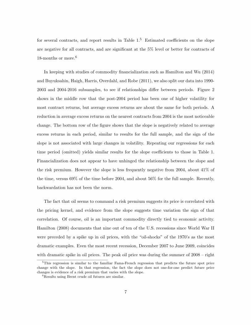
for several contracts, and report results in Table 1.5 Estimated coefficients on the slope

are negative for all contracts, and are significant at the 5% level or better for contracts of

18-months or more.6

In keeping with studies of commodity financialization such as Hamilton and Wu (2014)

and Buyuksahin, Haigh, Harris, Overdahl, and Robe (2011), we also split our data into 1990-

2003 and 2004-2016 subsamples, to see if relationships differ between periods. Figure 2

shows in the middle row that the post-2004 period has been one of higher volatility for

most contract returns, but average excess returns are about the same for both periods. A

reduction in average excess returns on the nearest contracts from 2004 is the most noticeable

change. The bottom row of the figure shows that the slope is negatively related to average

excess returns in each period, similar to results for the full sample, and the sign of the

slope is not associated with large changes in volatility. Repeating our regressions for each

time period (omitted) yields similar results for the slope coefficients to those in Table 1.

Financialization does not appear to have unhinged the relationship between the slope and

the risk premium. However the slope is less frequently negative from 2004, about 41% of

the time, versus 69% of the time before 2004, and about 56% for the full sample. Recently,

backwardation has not been the norm.

The fact that oil seems to command a risk premium suggests its price is correlated with

the pricing kernel, and evidence from the slope suggests time variation the sign of that

correlation. Of course, oil is an important commodity directly tied to economic activity.

Hamilton (2008) documents that nine out of ten of the U.S. recessions since World War II

were preceded by a spike up in oil prices, with the “oil-shocks” of the 1970’s as the most

dramatic examples. Even the most recent recession, December 2007 to June 2009, coincides

with dramatic spike in oil prices. The peak oil price was during the summer of 2008 – right

5This regression is similar to the familiar Fama-French regression that predicts the future spot pricechange with the slope. In that regression, the fact the slope does not one-for-one predict future pricechanges is evidence of a risk premium that varies with the slope.

6Results using Brent crude oil futures are similar.

7

before the collapse of Lehman Brothers. However, by December of 2007, the WTI spot

price was a very high $91.73 per barrel.

If the crude oil futures slope indirectly reveals information about the pricing kernel,

then perhaps the slope is informative of bond risk premia also? To investigate, we estimate

the regression

rnbond,t+1 − rft+1 = β0 + β1slopet + β2CPt + εt+1, (5)

where the left side is the excess return on a treasury bond portfolio with maturity n. We

add the factor CPt from Cochrane and Piazzesi (2005) to the right side, and consider

annual log holding period returns formed from monthly CRSP Treasury bond index data

from Jan. 1990 through Dec. 2003.7 Results in Table 2 show that a negative crude oil slope

predicts positive excess bond returns, with significance at the 5% level or better, depending

on bond maturity. As demonstrated elsewhere, the CPt factor also predicts excess bond

returns during this period. When combined with the slope both factors remain significant,

achieving R2 of around 0.5 for longer maturity bonds. In unreported additional regressions

we include summary macroeconomic factors from Ludvigson and Ng (2009), also shown to

predict excess Treasury bond returns, and find that the slope coefficient remains significant.

Results are sensitive to the holding period however, and are not as strong for, e.g., monthly

holding periods. We also included bond factors in the predictive regressions for crude oil

futures returns, and found that the bond factors do not significantly predict excess futures

returns. Finally, with the slope alone we extend our sample period through April 2016.

Table 3 shows that coefficients for most maturities remain significant at the 5% level or

better, although results for 1 and 2 year bonds especially are weaker once the 2008 financial

crisis is included.

Having established a relationship between the crude oil futures slope and risk premia

in futures and Treasuries, what remains is a direct connection to financial trade and risk-

7Cochrane and Piazzesi (2005) use Fama-Bliss bond indices, whereas we use similar CRSP Treasury bondindex data, which extends to synthetic bonds with longer maturity.

8

sharing. Important work along these lines is by Hong and Yogo (2012), who show that

commodity market open interest predicts excess returns on commodity futures and bonds,

and to a lesser degree excess stock and currency returns. They construct a composite

measure of growth in open interest across several commodity sectors, whereas we focus here

on oil. To illustrate the case for oil specifically, Figure 12 plots open interest and the slope

from Jan. 1990 through April 2016. We define OIt as the number of outstanding futures

contracts after removing a linear trend in logs, using data from the CFTC. Open interest

and the slope are positively correlated, although OIt appears to lag slopet, particularly

following sharp drops in the slope such as after the 2008 financial crisis.

Table 4 estimates

slopet = β0 + β1OIt + β2CIt + εt, (6)

adding CIt, the detrended percentage difference in commercial long versus short futures

contracts. This is similar to the composite commercial imbalance measure of Hong and

Yogo (2012). Each measure explains significant variation in the slope, with a combined R2

of around 20%. Although the slope does appear related to trade, we do not find OIt or

CIt to be strong direct predictors of excess returns on futures or bonds. This supports the

approach of Hong and Yogo (2012) to form smoothed composite measures of open interest

with less noise. However our model results will also suggest open interest has a more fragile

relationship to the risk premium than does the slope.

3 Model

We model an exchange or endowment economy as in (Lucas 1978). We specify a stochastic

process for the endowment growth. Specifically, we will have one good xt we think of as

the “numeraire” or composite commodity good. Our second good, which we calibrate to

be oil, we denote yt. We use the short-hand notation subscript-t to indicate conditional on

the history to date t. Similarly, we use Et and µt to indicate expectations and certainty

9

equivalents conditional on information to date-t. Heterogeneity in our setup will be entirely

driven by preference parameters. Beliefs across all agents are common.

We are interested in the Pareto optimal allocation or “perfect” risk sharing solution. So

with complete and frictionless markets, we focus on the social planner’s Pareto problem.

This means, for now, we need not specify the initial ownership of the endowment; we treat

xt and yt as resource constraints. The preferences, which we allow to differ across our two

agents, are recursive as in Epstein and Zin (1989) and Kreps and Porteus (1978). They

are characterized by three “aggregators” (see Backus, Routledge, and Zin (2005)). First,

a goods aggregator determines the tradeoff between our two goods. This is, of course,

a simplification since oil is not directly consumed. But the heterogeneity across our two

agents will capture that some of us are more reliant on the consumption of energy-intensive

products. The other two aggregators are the usual time aggregator and risk aggregator that

determine intertemporal substitution and risk aversion. Finally, the familiar time-additive

expected utility preferences are a special case of this setup.

3.1 Single Agent, Two Goods

To get started, consider a single-agent economy with two goods. In this setting the rep-

resentative agent consumes the endowment xt and yt each period. We model utility from

consumption of the “aggregated good” with a Cobb-Douglas aggregator,

At = A(xt, yt) = x1−γt yγt ,

with γ ∈ [0, 1]. The agent has Epstein-Zin recursive preferences over consumption of the

aggregated good,

Wt = W (xt, yt,Wt+1) = [(1− β)A(xt, yt)ρ + βµt(Wt+1)

ρ]1/ρ ,

µt(Wt+1) = Et[Wαt+1

]1/α.

10

Endowment growth follows a finite-state Markov process. Denote the state st, with the

probability of transitioning to next period state st+1 given by π(st, st+1), for st, st+1 ∈ S

with |S| finite. Growth in the numeraire good is ft+1 = f(st+1) = xt+1/xt, and similarly

for the oil-good gt+1 = g(st+1) = yt+1/yt.

With a little algebra, we can write the pricing kernel as

mt+1 =∂Wt/∂xt+1

∂Wt/∂xt(πt+1)

−1 = β

(xt+1

xt

)−1(At+1

At

)ρ( Wt+1

µt(Wt+1)

)α−ρ. (7)

Note that this is denominated in terms of the numeraire good (x). We can use mt+1 to

compute the price at t of arbitrary numeraire-denominated contingent claims that pay off

at t+1. Claims to oil good y at t are converted to contemporaneous numeraire values using

the spot price of oil,

Pt =∂Wt/∂yt∂Wt/∂xt

=γxt

(1− γ)yt. (8)

The pricing kernel and spot price can be used in combination to price arbitrary contingent

claims to either good.

The homogeneity of the Cobb-Douglas aggregator along with the standard homogeneity

of the time and risk aggregators allow us to rescale things so utility is stationary, similar to

Hansen, Heaton, and Li (2008), defining

Wt =Wt

A(xt, yt)=[(1− β) + βµt

(Wt+1A(ft+1, gt+1)

)ρ]1/ρ.

This uses the Cobb-Douglas property that A(xt+1,yt+1)A(xt,yt)

= A(ft+1, gt+1). Written in this

form, Wt is stationary and is a function only of the current state st. Similarly, substituting

Wt into the pricing kernel, we have

mt+1 = β (ft+1)−1 (A(ft+1, gt+1))

ρ

(A(ft+1, gt+1)Wt+1

µt(A(ft+1, gt+1)Wt+1)

)α−ρ. (9)

The pricing kernel depends on the current state st, via the conditional expectation in the

risk aggregator, and t+ 1 growth state st+1.

11

The price of oil depends on the relative levels of the two goods. However, changes in

the oil price will depend only on the relative growth rates:

Pt+1

Pt=ft+1

gt+1.

This implies the change in price depends only on the growth state st+1.

The advantages and limitations of a single agent single good representative agent model

are quite well known. For example, with a thoughtfully chosen consumption growth pro-

cess one can capture many salient feature of equity and bond markets (Bansal and Yaron

(2004)). Alternatively, one can look at more sophisticated aggregators or risk to match

return moments (Routledge and Zin (2010)). One could take a similar approach to extend

to a two-good case to look at oil prices and risk premia; see, e.g., Ready (2010). It would

require some work in our specific setup, since oil price dynamics would simply depend on

the growth state st in combination with constant preference parameter γ.

Instead we introduce a second, but similar, agent. The dynamics of the risk sharing

problem we discuss next will provide us a second state variable, besides st+1, to generate

realistic time variation in the oil risk premium. This also lets us look at the portfolios and

trades the two agents choose to make. Lastly, note that the single agent case in this section

corresponds to the boundary cases in the two-agent economy, where one agent receives zero

Pareto weight (or has no wealth).

3.2 Two Agents, Two Goods

Consider a model with two agents, leaving the two-good endowment process and recursive

preference structure unchanged. We allow the two agents to have differing parameters

for their goods, risk, and time aggregators. Denote the two agents “1” and “2”; these

subscripts will denote the preference heterogenity and the endogenous goods allocations.

The risk sharing or Pareto problem for the two agents is to allocate consumption of the

12

two goods across the two agents, such that cx1,t + cx2,t = xt and cy1,t + cy2,t = yt. Agent one

derives utility from consumption of the aggregated good A1(cx1,t, c

y1,t) = (cx1,t)

1−γ1(cy1,t)γ1 .

The utility from the stochastic stream of this aggregated good has the same recursive form

as above,

Wt = W (cx1,t, cy1,t,Wt+1) =

[(1− β)A1(c

x1,t, c

y1,t)

ρ1 + βµ1,t(Wt+1)ρ1]1/ρ1

,

µ1,t(Wt+1) = Et[Wα1t+1

]1/α1 .

(10)

Agent two has similar preference structure with A2(cx2,t, c

y2,t) = (cx2,t)

1−γ2(cy2,t)γ2 and recur-

sive preferences

Vt = V (cx2,t, cy2,t, Vt+1) =

[(1− β)A2(c

x2,t, c

y2,t)

ρ2 + βµ2,t(Vt+1)ρ2]1/ρ2

,

µ2,t(Vt+1) = Et[V α2t+1

]1/α2 .

(11)

The idea is that the two agents can differ about the relative importance of the oil good,

risk aversion over the “utility lotteries”, or the intertemporal smoothing. Recall that with

recursive preferences all of these parameters will determine the evaluation of a consumption

bundle. “Oil risk” does not just depend on the γ parameter since it involves an intertem-

poral, risky consumption lottery. We give the two agents common rate of time preference

β.8

The two-agent Pareto problem is a sequence of consumption allocations for each agent

{cx1,t, cy1,t, c

x2,t, c

y2,t} that maximizes the weighted average of date-0 utilities subject to the

aggregate resource constraint which binds at each date and state:

max{cx1,t,c

y1,t,c

x2,t,c

y2,t}

λW0 + (1− λ)V0

s.t. cx1,t + cx2,t = xt and

cy1,t + cy2,t = yt for all st,

where λ determines the relative importance (or date-0 wealth) of the two agents. Even

though each agent has recursive utility, the objective function of the social planner is not

8Differing β’s are easy to accommodate but lead to uninteresting models since the agent with the largerβ quickly dominates the optimal allocation. See, e.g., Yan (2008).

13

recursive, except in the case of time-additive expected utility. We can rewrite this as a

recursive optimization problem, following Lucas and Stokey (1984) and Kan (1995):

J(xt, yt, Vt) = maxcx1,t,c

y1,t,Vt+1

[(1− β)A1(c

x1,t, c

y1,t)

ρ1 + βµ1,t(J(xt+1, yt+1, Vt+1))ρ1]1/ρ1

s.t. V (xt − cx1,t, yt − cy1,t, Vt+1) ≥ Vt.

(12)

The optimal policy involves choosing agent one’s date t consumption, cx1,t, cy1,t and the

resource constraint pins down agent two’s date t bundle. In addition, at date t we solve for

date t+1 “promised utility” for agent two. This promised utility is a vector, since we choose

one for each possible growth state st+1. Making good on these promises at date t+1 means

that Vt+1 is an endogenous state variable we need to track. That is, optimal consumption

at date t depends on the exogenous growth state st and the previously promised utility Vt.

Finally, note that the solution to this problem is “perfect” or optimal risk sharing. Since

we consider complete and frictionless markets, there is no need to specify the individual

endowment process.

Preferences are monotonic, so the utility-promise constraint will bind. Therefore with

optimized values, we have Wt = W (cx1,t, cy1,t,Wt+1) = J(xt, yt, Vt) and Vt = V (xt − cx1,t, yt −

cy1,t, Vt+1). Optimality conditions imply that the marginal utilities of agent one and agent

two are aligned across goods and intertemporally:

mt+1 = β

(cx1,t+1

cx1,t

)−1(A1,t+1

A1,t

)ρ1 ( Wt+1

µ1,t(Wt+1)

)α1−ρ1

= β

(cx2,t+1

cx2,t

)−1(A2,t+1

A2,t

)ρ2 ( Vt+1

µ2,t(Vt+1)

)α2−ρ2.

(13)

Recall that beliefs are common across the two agents so probabilities drop out. We can

use this marginal-utility process as a pricing kernel. Optimality implies agents agree on the

price of any asset.

Similarly, the first-order conditions imply agreement about the intra-temporal trade of

the numeraire good for the oil good. Hence the spot price of oil:

Pt =γ1c

x1,t

(1− γ1)cy1,t=

γ2cx2,t

(1− γ2)cy2,t. (14)

14

As in the single agent model, homogeneity allows for convenient rescaling. The analogous

scaling in the two-agent setting is

cx1,t =cx1,txt

, cy2,t =cx2,txt

= 1− cx1,t,

cy1,t =cy1,tyt

, cy2,t =cy2,tyt

= 1− cy1,t.

The c’s are consumption shares of the two goods. We also scale utility values using their

respective goods aggregators,

Wt =Wt

A1(xt, yt), Vt =

VtA2(xt, yt)

.

Notice we scale the utilities by the total available goods, not just the agent’s share. This

has the advantage of being robust if one agent happens to (optimally) get a declining share

of consumption over time.9 Plugging these into the equation (13), and we can state the

pricing kernel as

mt+1 =

β

(ft+1c

x1,t+1

cx1,t

)−1(A1(ft+1c

x1,t+1, gt+1c

y1,t+1)

A1(cx1,t, cy1,t)

)ρ1 (A1(ft+1, gt+1)Wt+1

µ1(A1(ft+1, gt+1)Wt+1)

)α1−ρ1

,(15)

or equivalently from the perspective of agent two. In the one-agent case, the pricing kernel

depends on the current growth state st and the future growth state st+1. In the two agent

case, the pricing kernel depends on both the growth state and the scaled utility of agent

two currently (st, Vt) and in the future (st+1, Vt+1).

3.3 Financial Prices

We can now use the pricing kernel to price assets and calculate their returns. To start,

we can look at the values of each agent’s consumption streams, which measure individual

wealth. Agent one’s claim to numeraire consumption good x has value at date t

Cx1,t = Et

[ ∞∑τ=t

mτ cx1,τ

]. (16)

9In particular, we use these normalizations to make the optimization problem in Equation (12) indepen-dent of current levels of xt and yt.

15

This is the cum dividend value, including current consumption.

We conjecture that

Cx1,t =cx1,tW

ρ1t

(1− β)Aρ11,t, (17)

which is easily verified using the pricing kernel definition in equation (13). Substituting our

normalizations,

Cx1,t =

(cx1,tW

ρ1t

(1− β)A1(cx1,t, cy1,t)

ρ1

)xt. (18)

Note that the price of the claim to numeraire consumption is conditionally independent of

the level of aggregate oil consumption; that is, the ratio Cx1,t/xt depends only on our state

variables st and Vt. To price the claim to the oil consumption good, we use the oil price to

convert to units of numeraire good:

Cy1,t = Et

[ ∞∑τ=t

mτPτ cy1,τ

]=

γ11− γ1

Cx1,t.

Again, aggregate oil consumption does not play a role, and the ratio Cy1,t/xt depends only

on the state variables st and Vt. Lastly, summing the value of the numeraire and oil claim

we calculate the total wealth of agent one:

C1,t = Cx1,t + Cy1,t =1

1− γ1Cx1,t. (19)

By equivalent logic, the values of agent two’s consumption claims are

Cx2,t =

(cx2,tV

ρ2t

(1− β)A2(cx2,t, cy2,t)

ρ2

)xt.

Cy2,t =γ2C

x2,t

1− γ2

C2,t =Cx2,t

1− γ2

With the wealth of each agent, we can define aggregate wealth in the numeraire sector,

Cxt = Cx1,t + Cx2,t, (20)

16

in the oil sector,

Cyt =γ1C

x1,t

1− γ1+γ2C

x2,t

1− γ2, (21)

and the overall wealth in the economy,

Ct =Cx1,t

1− γ1+

Cx2,t1− γ2

. (22)

Bond prices and the risk free rate all follow from the pricing kernel in the usual way.

Define the price of a zero-coupon bond recursively as

Bt,n = Et[mt+1Bt+1,n−1], (23)

where Bt,n is the price of a bond at t paying a unit of the numeraire good at period t+ n,

with the usual boundary condition that Bt,0 = 1.

The futures price of the oil good, y, is defined as follows. Ft,n is the price agreed to in

period t for delivery n period hence. Futures prices satisfy

0 = Et[mt+1(Ft+1,n−1 − Ft,n)]

⇒ Ft,n = (Bt,1)−1Et[mt+1Ft+1,n−1],

(24)

with the boundary condition Ft,0 = Pt.

3.4 Portfolios

One interesting feature of a multi-agent model is that we can look directly at the role

of financial markets in implementing the Pareto optimal allocations, by defining a set of

tradeable financial assets that dynamically complete the market. In particular, we are

interested in how oil futures are traded in such a setting. We defer that specific question to

our numerical example of the model, since we lack analytical expressions for futures prices.

However, we can look analytically at how “equity” claims can implement the optimal

allocations. Recall that Cxt is the value of a claim to the stream of numeraire good and Cyt is

17

the value of the claim to the stream of the oil good. We think of these as (unlevered) claims

to equity in the numeraire and oil sectors, and normalize the shares outstanding in each

sector to one. Suppose these were traded claims in the economy. Is there a portfolio of φx1,t

shares in numeraire and φy1,t shares in oil that implement optimal consumption for agent

one, with 1 − φx1,t and 1 − φy1,t shares optimal for agent two? This amounts to replicating

the optimal wealth process for each agent using the equity claims. It turns out this is easy

to solve. The agents’ budget constraint are:

C1,t = φx1,tCxt + φy1,tC

yt

C2,t = φx2,tCxt + φy2,tC

yt

Substitute in the definition of the aggregate value of the numeraire sector in equation (20)

and oil sector in equation (21). The key here is that for each agent, the value of the oil

consumption stream is proportional to the value of the numeraire stream, i.e.,

Cy1,tCx1,t

=γ1

1− γ1,Cy2,tCx2,t

=γ2

1− γ2.

This all implies, for agent one:

Cx1,t =(1− γ1) ((−γ2Cxt + (1− γ2)Cyt )

γ1 − γ2(25)

and

φx1,t =−γ2

γ1 − γ2(26)

φy1,t =1− γ2γ1 − γ2

. (27)

Equivalent results hold for agent two. Note that shareholdings are constant. As we will

see in the numerical section in a moment, optimal consumption for the two agents, and the

implied prices and asset returns, have many interesting dynamic properties. These prop-

erties depend on the interaction of preferences over goods, intertemporal substitution, and

18

risk-aversion over states. However the homogeneity of the preference structure means that

portfolio policies are “buy and hold” if equity claims to each sector are tradeable. Further-

more, equity portfolios depend only on the agents’ relative preference for oil consumption.

These results caution against taking portfolio holdings as an adequate summary of agent

attitudes towards risk.

While this result is interesting, perhaps it is not all that practical. The equity positions

implied by Equation (27) are extreme for reasonable values of γ1 and γ2, for example if

agents have relatively similar preferences over goods. And of course not all claims to oil

production revenues are financed through publicly traded equity. In the numerical section,

next, we look at portfolio policies that implement optimal consumption using oil futures

contracts. This also gives us a perspective on open-interest dynamics.

4 Numerical Example

The recursive Pareto problem is hard to characterize analytically, so we look at a numerical

example. The goal of the example is to capture enough of the salient features of the data to

be quantitatively informative, while remaining simple enough to inspect results. In single

agent endowment models, obtaining a reasonable equity premium requires either highly

persistent risks to consumption growth as in Bansal and Yaron (2004), or rare disaster-like

risk as in Barro (2009). Time-variation in risk premiums requires stochastic volatility (e.g.,

Bansal and Yaron (2004)) or variation in the likelihood of disaster (e.g, Wachter (2013)).

For simplicity we assume a four state Markov process for annual growth, described in Table

5, with growth in x as f(s) and growth in y as g(s). Notice that the process has a disaster-

like risk in states one and four. In our two-agent economy, which of those states is the

bigger concern will drive risk premiums. Endogenous variation in the wealth distribution is

an additional source of time-variation in the risk premium, by weighting aggregate concern

towards one disaster state or the other.

19

The parameters in Table 5 imply that the numeraire (x) and oil (y) processes have uncon-

ditional mean growth rates of 2% per year. Unconditional standard deviations of numeraire

and oil consumption growth are 3% and 6%, respectively. The unconditional correlation

in growth rates is positive, at 0.44. Historically, oil consumption represents approximately

4% of US GDP (Hamilton (2008)). In our model this characteristic is governed chiefly by

the choice of goods aggregation parameters. All preference parameters are listed in Table

6. In the Cobb-Douglas aggregator we use γ1 = 0.03 and γ2 = 0.06. This gives agent two a

greater preference for oil consumption than agent one, while keeping oil within a plausible

range of the 4% historical average. Risk aversion (αi) and intertemporal substitution (ρi)

parameters address the risk premiums on equity and oil futures. We have selected these

parameters to maintain a plausibly high but variable equity risk premium, while allowing

for more dramatic variation in the oil futures risk premium. Specifically, a single agent

economy with just agent one would have an equity risk premium of about 2% per year,

whereas with just agent two the equity premium is about 4%. Not surprisingly, our simple

four state Markov process is too coarse a description to completely capture all aspects of

equity returns.10 Notice that agent one has a higher risk aversion coefficient. This does

not directly translate to higher “risk aversion” (and a higher equity risk premium) since

the preferences include, recursively, the sensitivity to oil risk. In some sense, agent two

faces “more risk” from the higher exposure to the oil-good. This interplay is helpful for

understanding the numerical results that follow.

Since the model is stationary in growth, initial levels of x0 and y0 do not impact returns

or risk premia. The level of the spot price, however, depends on the ratio of oil and

numeraire, as in equation (14). We choose the (arbitrary and innocuous) initial level of

x0 and y0 so that spot prices are at a familiar per-barrel level (e.g., $60/bbl). However,

since the endowment levels of xt and yt are not cointegrated, the spot price of oil in this

specification is non-stationary. Since we focus on returns in what follows this plays no

10We abstract from many of the usual model characteristics such as dividends being distinct from con-sumption, leverage, and so on.

20

role.11 Whether or not the spot price of oil is in fact stationary is an interesting question

that involves the interplay of technological progress affecting oil demand and supply. A

gallon of gasoline yields more miles in 2015 than 1971 and changes in shale oil (and gas)

technology have had a large impact on supply. This is a central issue in resource economics

that more carefully considers the long run implications of “peak oil,” is an addressed in

Ready (2014) and David (2015), but is a side issue in our setting.

With different parameter values, our model could easily be used to study markets other

than oil. For example, its basic structure is similar to the international finance model in

Colacito and Croce (2013), which features two agents, representing countries, with hetero-

geneous preferences over foreign and domestic consumption goods. By restricting the form

of preference heterogeneity and the growth process, their model takes on useful features

such as a stationary wealth distribution, as proved in Colacito and Croce (2014). But mod-

eling the oil market requires more general preference heterogeneity than these restrictions

allow. For example, we cannot assume that agents have symmetrical goods preferences

(γ1 = 1−γ2), because it would unrealistically imply oil is greater than 50% of consumption

expenditures for one of the agents. Neither can we assume α1 = α2 and ρ1 = ρ2, because

we could not obtain the variety of risk premia we seek.

For the oil futures risk premium, our goal is to generate variation that is in a range

consistent with recent data. Hamilton and Wu (2014), for example, suggests an annualized

risk premium to a long position in the 8-week contract of around 4% in 1990, falling to

around -5% in 2011. Our endowment and preference parameters generate an unconditional

oil futures risk premium of about 3% in an economy populated solely by agent one, and a -2%

unconditional risk premium under an economy of only agent two. We can then investigate

11It is easy to specify a growth process with a stationary oil price by specifying the growth dynamics ofthe numeraire and for the ratio of oil-to-numeraire. While the results are broadly similar in such a setupit is harder to generate sizable risk premiums for oil. Roughly, imposing the assumption that oil and thegeneral economy are co-integrated implies that “oil risk” is smaller. This is analogous to why our four stateMarkov model looks disaster-like rather than long-run-risk. The long run risk aspect is hard to capture ina small number of states.

21

how the dynamic risk-sharing properties of the model might endogenously generate some

of the change we see in risk premiums over the 1990 to 2015 period, without any structural

breaks.

4.1 Wealth and consumption

With the growth process in Table 5 and the preference parameters in Table 6, we solve

the dynamic recursive Pareto problem outlined in (12). The exogenous Markov growth is

characterized by its current state, s. The key endogenous state variable in the solution of

the Pareto problem is the promised continuation utility level for agent two, V . Since V is

bounded and positive, we normalize this state variable to the [0, 1] interval.12

Figure 4 plots the oil consumption share, the numeraire good consumption share, and

the wealth share as a function of the endogenous promised utility level. The figure integrates

across the exogenous growth state, s, at the unconditional stationary probabilities. In this

example, the shares of aggregate wealth (bottom panel) are nearly linear in V . So a value of

V = 0.25 corresponds to agent two owning roughly 25% of aggregate wealth. The curvature

in the top panel of Figure 4 highlights the two agents’ differing preference for oil: agent two

has a stronger preference for oil, and so tends to get a disproportionate share.

Risk sharing models are often non-stationary, in the sense that the long horizon has one

agent dominating the economy; see, e.g., Yan (2008) and Anderson (2005). In our numerical

example, V drifts towards one. We do not derive analytical survival or extinction conditions

for the general case with heterogeneous Epstein-Zin preferences and multiple goods, and to

12 Although an agent’s utility may grow as the economy expands, recall that Vt = VtA2(xt,yt)

is bounded for

any xt and yt. However the domain of V is determined in equilibrium based on the model parameters. Itsminimum value is 0, and its maximum Vmax corresponds to the case where agent two consumes the aggregateoutput of each good, i.e. cx2,t = xt, c

y2,t = yt in perpetuity. This lets us normalize by dividing V by Vmax,

to obtain a state variable between zero and 1. To be precise, since Vmax depends upon the current growthstate, we normalize V by its conditional maximum.

22

our knowledge such results are not presented in prior work.13 Although simulations suggest

that agent two will dominate the economy at long-horizons, the dynamics of V are slow and

low frequency relative to the exogenous Markov growth process. Figure 5 shows the density

of V over long horizons from of 10 and 100 years, starting at an initial value of V0 = 0.05.

As we discuss later, we choose the low initial V0 to illustrate how a drift in wealth share may

produce apparent trends in open interest, the spot price, and the futures risk-premium.

4.2 Risk premia

Prices and conditional expected returns and risk premiums depend on the exogenous Markov

growth state, s and the endogenous state variable V , effectively the wealth share of agent

two. We use our numerical example to look at behavior conditional on each of the exogenous

and endogenous state variables. Figure 6 plots mean oil price and returns conditional on the

wealth share V . They are “mean” values in the sense that we integrate out the exogenous

state s at its stationary (unconditional) likelihoods, holding constant the wealth share.

Notice that the (mean) oil spot price is increasing in the wealth share of agent two. This

reflects, of course, agent two’s greater preference for the oil good. The risk premium in oil

futures is positive for low levels of V and is negative for higher levels V . That is, when

agent one has a high wealth share (low V ), oil futures have a positive risk premium and

when agent two is more wealthy the risk premium is negative. Interestingly, asset returns

for the numeraire good, the risk free rate and the equity risk premium, are not monotonic in

the wealth share. Near a wealth share of approximately 0.3, the equity premium is highest,

the risk free rate is at its lowest, and the oil risk premium is near zero.

Before digging into the mechanism that is driving these results, we characterize our

example along the same lines as the returns data, starting with contracts of differing matu-

13Colacito and Croce (2014) present an example of a stationary two-agent economy with Epstein-Zinpreferences and two goods, but prove stationarity under several assumptions not imposed in our study, suchas a symmetrical growth process, and preference heterogeneity limited to symmetrical differences in thegoods parameter value.

23

rity. Figure 7 presents the term-structure of oil futures risk premiums. Notice that the risk

premiums are lower when agent two has a larger wealth share (larger V ) at all horizons, as

we saw in Figure 6 for the near-term contract. The fact that risk premiums are declining

in maturity is interesting. In an economy dominated by agent one (low V ), the largest risk

premium is positive and at the short end. In contrast, in the economy with a higher wealth

share for agent two (high V ), the sizable risk premium is negative and at the long end.

Hitzemann (2015) emphasizes oil-sector exposure to long run risk, which is not included in

our model, as a mechanism that generates a risk premium increasing in maturity. Although

disaster risk and long run risk have not yet been studied in a combined oil economy frame-

work, the natural supposition is that the two sources of risk would offset each other’s effects

on the term structure of risk premiums. Historical average excess returns show a relatively

flat term structure overall, particularly for contracts out 12 months or more, as illustrated

in Figure 2.

Turning to the conditional risk premiums, Figure 8 plots the oil risk premium on the

short-horizon two year contract, conditional on both the endogenous wealth share, V , and

the endogenous growth state, s. This shows that the risk premium is low in state s = 1, when

oil is growing relatively scarce, and vice versa for state s = 4, when oil is growing relatively

abundant. We cannot directly observe analogous growth states in the data. However we

can condition on the slope of the futures curve in the model. Table 7 shows risk premiums

conditional on the slope of the futures curve in the model, analogous to Figure 2 for the

data. Note that the risk premium is conditionally higher, and generally positive, when the

futures slope is negative.

Table 8 uses the current slope to predict excess futures returns, via regressions equivalent

to those performed on the data. Regression coefficients are computed via simulation, with

an initial value of V as specified in the table. We report average coefficients from 10,000

paths of 100 periods each. As in the data, in Table 1, the coefficient on the slope is negative

for all contracts, so a downward sloping futures curve implies higher expected excess futures

24

returns. However t-statistics from the model regressions are not significant at conventional

levels for larger values of V . That is, the slope becomes a less effective predictor of excess

returns as agent 2 becomes wealthier. The futures curve is also less frequently downward

sloping for larger V , e.g., the slope is negative about 80% of the time in for the smallest V

versus only 6% of the time for the largest V . These results illustrate that apparent empirical

regularities in the futures market may be fragile if trade reflects heterogeneous preferences,

because wealth may shift between types over time.

In the data, we also examined the cross-market relationship between crude oil futures and

bonds. Figure 10 shows the term structure of real interest rates conditional on the wealth

share, V . For most values of V the term structure is relatively flat, with slightly downward

sloping rates around 1.25% for V = 0.35, and slightly upward sloping rates around 2.25%

for V = 0.95. The exception is V = 0.05, which is steeply downward sloping. Ang, Bekaert,

and Wei (2008) estimate that unconditional real interest rates are relatively flat around

1.3%, with some regimes in which the real rate curve is steeply downward sloping. They

attribute the upward sloping nominal term structure to an inflation risk premium, which of

course we cannot replicate without adding money to our model. However we can still see

how (real) bond risk premia in our model relate to the slope of the crude oil futures curve.

Recall that Table 2 and Table 3 show how the Treasury bond risk premium correlated

with the oil risk premium, as measured by the futures slope. Table 10 replicates the re-

gression of annual excess bond returns on the futures slope, reporting average coefficients

for 10,000 paths of 100 periods each. We do see dependence on the futures slope, but with

the opposite correlation to the data. In the data, particularly the 2004 period, a negative

slope was indicative of a larger bond risk premium. Possibly the negative coefficient in the

data results from the futures curve predicting the inflation risk premium. One aspect the

model example seems to capture is that the degree of correlation – as seen in Table 9 by the

difference between the term premium conditional on a positive or negative oil futures curve

– varies over time with the endogenous wealth share state. Notice in the table that around

25

V = 0.35 the relationship changes from a higher term premium with positive slope to a

higher term premium with negative slope. This illustrates that the relationship between

risk premia across markets may not be robust over time, even in the absence of structural

breaks.

4.3 Why?

The key driver in the numerical example is that, on average, agent one views a long position

in oil as risky and requires a positive risk premium, whereas agent two views the long position

in oil as a hedge and accepts the negative risk premium as insurance. Why is that? Our

four state growth process in Table 5 has the feel of a “disaster” model. States 1 and 4 are

the bad-outcome states. State 1 has low numeraire growth, very low oil growth, and a rising

price of oil. This state loosely resembles a recession induced by an oil-supply shock. State

4 has very low numeraire growth, plentiful oil growth, and a falling price of oil. This is

reminiscent of a deep recession whose roots do not lie in oil. The two agents in the example

rank these states differently.

We can see the agents’ ranking of the growth states by looking at the state price densities.

Recall that optimality aligns the two agents’ marginal rates of substitution, state-by-state,

as in equation (13). The state price density, mt+1,t, is for moving to growth state st+1 and

wealth share Vt+1 given the current st and wealth share Vt. Figure 9 captures the salient

informaton in the state price density by plotting the average mt+1,t for each of the four

growth states st+1, integrating out the current growth state.14 The figure lets us look at

state prices for the four growth states while varying the wealth share of agent two; the left

of the graph is an economy of mostly agent one and the right is an economy of mostly agent

two.

Denote the state prices shown in Figure 9 as Ms. The two lower lines of Figure 9,

14The figure looks very similar across various alternative averaging.

26

M2 and M3, are both small. The two agents view these states similarly and as equally

bountiful; these prices vary little as the wealth share moves. The upper lines are for states

1 and 4. Both of these states are “bad,” and weigh heavily on asset returns. For agent one,

the low-volume-oil consumer, state 4 is the worst: for V near 0, M4 > M1. In state 4 the

spot price of oil decreases, hence a long position in oil has a low payoff. Therefore, to agent

one, oil futures are risky and command a positive risk premium. For agent two, the agent

with the higher dependence on oil, the low growth of oil in state 1 dominates: for V near

1, M1 > M4. In state 1 the spot price of oil increases. To agent two, a long position in

oil futures has a large payoff precisely when the marginal rate of substitution is high. This

hedge, in equilibrium, produces the negative risk premium to a long position in oil.

For ranges of the wealth share that are not near the boundary, we can see the impact

of risk sharing. For V around 0.35, the risk premium on oil, at the short end, is close to

zero; see Figures 6 and 7. In our example, this is where “hedgers” and “speculators” have

equal demand. Looking back at Figure 6, this is near the region where the risk free rate is

particularly low and the equity risk premium is at its highest. Here, it seems, with the oil

risk sharing as large as possible (i.e. a zero oil risk premium), the scope for risk sharing in

the numeraire good is smaller, and hence the two numeraire claims reflect this. The risk

free rate is low, and the equity premium is high. The discussion here focuses on one-period

gambles, as captured in Figure 9. Risk premiums are more complicated a longer horizons.

Both agents view the long-oil futures position as more of a hedge at longer horizons. The

risk premiums in Figure 7 are generally downward sloping.

4.4 Portfolios and open interest

As we saw in Section 3.3, when claims to aggregate consumption of the numeraire and oil are

traded in financial markets, then the agents can implement their optimal consumption plans

with a constant buy-and-hold portfolio. In our example, agent one would hold 2 shares of

27

the claim to aggregate numeraire consumption (akin to a broad equity portfolio excluding

the oil sector), and roughly −32.3 shares of a claim to oil consumption (say shares in Exxon,

Chevron, and so on). The aggregate supply of each of these two assets is normalized to

one. So agent two’s portfolio is short one share of the equity claim and is long 33.3 shares

of the oil claim.15 Neither of these portfolios is particularly practical. In reality investors

are unable to trade a claim to aggregate consumption of oil. Much of world oil production

is in state-owned enterprises (e.g., Saudi Aramco, PDVSA) that are not publicly traded.

In practice, we see trade in futures contracts. And, as noted earlier, a large increase in

trading volume occurred post 2004. We can implement of our Pareto-optimal allocations

using futures contracts to (dynamically) complete the market. With four growth states,

we can do this with four assets. Here, we use a claim to aggregate consumption of both

goods C (call this “equity”), the one-period risk free bond B1, and two fully-collateralized

oil futures contracts. We use the one and two year horizon contracts (labeled F1 and F2,

respectively).

Figure 11 shows each agent’s optimal portfolios for a range of wealth shares of agent

two (the endogenous state-variable V ). Market clearing implies that agent two’s holdings

of futures contracts are the mirror image of agent one’s: the bond and the futures contracts

are in zero net-supply, whereas equity has a net supply of one. The equity claim, denoted

C in Figure 11, mostly reflects the relative wealths of the two agents. Recall that it is agent

two who most desires to hedge the oil-price risk. Hence, agent two’s portfolio is long F1 –

the futures contract that is most sensitive to the oil spot price. It is interesting that getting

the right sensitivity to the price of oil requires a long position in F1 and a short position in

the longer-dated contract F2: a calendar spread. So the overall hedging motive of a trader

could easily be misinterpreted based on the direction of trade in a single contract.

There has been extensive policy debate around increases in open interest in the oil

15The portfolios specified are nevertheless equivalent to the dominant agent holding one share of eachstock when V → 0 or V → 1.

28

futures market. Figure 12 plots open interest, defined here as the absolute value of agent

one’s position. Not surprisingly, open interest is small when the economy is dominated

by one agent (V near 0 or 1). Interestingly, the open interest is largest near V = 0.35.

This corresponds to where the oil risk premium is zero – the point where “hedgers” and

“speculators” are equally balanced. Recall that the price of oil is increasing in the share

of wealth for agent two, as shown in the right panel of Figure 12. So in this example, an

increase in open interest and an increase in the oil price occur as V moves, say, from 0.05

to 0.35.

In the data, we also saw in Table 4 that open interest is positively correlated with the

futures slope, which is an indicator of the risk premium. However we noted that open

interest does not directly predict excess futures returns at a statistically significant level.

Table 11 shows that open interest is also significantly, but imperfectly, positively correlated

with the futures slope in the model. Variation in open interest partially reflects the state

of nature s, but as we see in Figure 12, open interest also varies nonmonotonically with

V . The futures risk premium varies with both s and V . As a result, based on simulated

regressions, open interest does not directly predict excess futures returns at a statistically

significant level in the model either.

4.5 Wealth Dynamics

As we noted previously while examining Figure 5, the wealth share of agent two, V has

positive drift in our example. Quantitatively, what are the effects of this drift, and how

do they compare to data? Figure 13 shows an average path (across 10,000 simulations) for

agent 2 wealth share (V ), the spot price, the futures risk premium, and open interest over

a 50 year horizon. Open interest and the risk premium use the one-year (nearest) contract.

As the drift in wealth share is relatively slow, we choose the initial V to be in a region

where the economy is more sensitive to changes in the wealth distribution. We initialize

29

the simulation at V = 0.05. This is an economy dominated by agent one. Agent one has

a lower preference for oil, so the initial spot price is low. Also, since V = 0.05 has one

dominant agent, open interest is low. As the economy evolves, V increases and agent two

has a larger role. Over the 50 year horizon, the expected oil price roughly doubles, as does

expected open interest as a fraction of total wealth. The risk premium falls by about 1/3,

a change consistent in direction with split sample averages for near-to-maturity contracts,

although not for long-dated contracts.16

The results suggest that, at least over a horizon of decades, the wealth distribution

is an important driver of the amount of trade in futures, and the futures risk premium.

And indeed there would be changes in goods market prices coinciding with financial market

changes, although the magnitude of these must be interpreted with care. Most of the

expected increase in the spot price results from the correlated growth process for the oil and

non-oil goods: the increase in spot price attributable to the change in wealth distribution

is about 8%. So the run up in oil prices before 2008, for example, would have to stem from

the relative growth in aggregate consumption of oil, not from a shift in wealth alone.

5 Conclusion

We have focused on heterogeneous attitudes towards oil risk as an important driver of oil

risk premium dynamics, price dynamics, and trade evident in the data. To attack this ques-

tion, we look at the frictionless consumption sharing problem for two agents with different

attitudes towards consumption risk and, specifically, the oil-component of consumption.

The solution lets us look at consumption and wealth paths and the implications for risk

premiums. Changes in market behaviour follow shifts in the wealth distribution, which

are endogenous and Pareto optimal. In a numerical example, we generate in expectation

16In our example, long-dated contracts would also see a decline in risk premium on average in the simu-lation.

30

rising oil prices, decreasing risk premiums, and increasing open interest. However the exam-

ple suggests that consumption or wealth share dynamics are unlikely to account for rapid

variation oil futures market dynamics, except perhaps for open interest.

31

References

Anderson, E. W. (2005): “The dynamics of risk-sensitive allocations,” Journal of Economic The-ory, 125(2), 93 – 150.

Ang, A., G. Bekaert, and M. Wei (2008): “The term structure of real rates and expectedinflation,” The Journal of Finance, 63(2), 797–849.

Backus, D. K., B. R. Routledge, and S. E. Zin (2005): “Exotic Preferences for Macroe-conomists,” in NBER Macroeconomics Annual 2004, ed. by M. Gertler, and K. Rogoff, vol. 19,pp. 319–391. MIT Press, Cambridge, MA.

(2008): “Recursive Risk Sharing: Microfoundations for Representative-Agent Asset Pric-ing,” Carnegie Mellon Working Paper.

(2009): “Who Holds Risky Assets?,” Carnegie Mellon Working Paper.

Baker, S. D. (2015): “The Financializatin of Storable Commodities,” Discussion paper, Universityof Virginia.

Bansal, R., and A. Yaron (2004): “Risks for the long run: A potential resolution of asset pricingpuzzles,” The Journal of Finance, 59(4), 1481–1509.

Barro, R. J. (2009): “Rare Disasters, Asset Prices, and Welfare Costs,” The American EconomicReview, 99(1), pp. 243–264.

Buyuksahin, B., M. Haigh, J. Harris, J. Overdahl, and M. Robe (2011): “Fundamentals,trader activity and derivative pricing,” Discussion paper, American University.

Carlson, M., Z. Khokher, and S. Titman (2007): “Equilibrium Exhaustible Resource PriceDynamics,” Journal of Finance, 62(4), 1663–1703.

Casassus, J., P. Collin-Dufresne, and B. Routledge (2007): “Equilibrium CommodityPrices with Irreversible Investment and Non-linear Technologies,” Hass Working Paper.

CFTC (2008): “Staff Report on Commodity Swap Dealers and Index Traders with CommissionRecommendations,” Discussion paper, Commodity Futures Trading Commission.

Cochrane, J. H., and M. Piazzesi (2005): “Bond Risk Premia,” The American EconomicReview, 95(1), 138–160.

Colacito, R., and M. M. Croce (2013): “International asset pricing with recursive preferences,”The Journal of Finance, 68(6), 2651–2686.

Colacito, R., and M. M. Croce (2014): “Recursive allocations and wealth distribution withmultiple goods: Existence, survivorship, and dynamics,” Discussion paper, University of NorthCarolina.

David, A. (2015): “Exploration Acivity, Long Run Decisions and the Risk Premium on EnergyFutures,” Discussion paper, University of Calgary.

Epstein, L. G., and S. E. Zin (1989): “Substitution, Risk Aversion, and the Temporal Behaviorof Consumption and Asset Returns: A Theoretical Framework,” Econometrica, 57(4), 937–969.

Fama, E. F., and K. R. French (1987): “Commodity Futures Prices: Some Evivedence onForecast Power, Premiums and the Theory of Storage,” Journal of Business, 60(1), 55–73.

Hamilton, J. (2009): “Causes and Consequences of the Oil Shock of 2007-08,” NBER WorkingPaper.

32

Hamilton, J. D. (2008): “Oil and the Macroeconomy,” in The New Palgrave Dictionary of Eco-nomics, ed. by S. N. Durlauf, and L. E. Blume. Palgrave Macmillan.

Hamilton, J. D., and J. C. Wu (2014): “Risk premia in crude oil futures prices,” Journal ofInternational Money and Finance, 42, 9–37.

Hansen, L., J. Heaton, and N. Li (2008): “Consumption Strikes Back? Measuring Long-RunRisk,” Journal of Political Economy, 116(2), 260–302.

Hirshleifer, D. (1988): “Residual Risk, Trading Costs, and Commodity Futures Risk Premia,”Review of Financial Studies, 1(2), 173–193.

Hirshleifer, D. (1990): “Hedging pressure and futures price movements in a general equilibriummodel,” Econometrica: Journal of the Econometric Society, pp. 411–428.

Hitzemann, S. (2015): “Macroeconomic Fluctuations, Oil Supply Shocks, and Equilibrium OilFutures Prices,” Discussion paper, Ohio State University.

Hong, H., and M. Yogo (2012): “What does futures market interest tell us about the macroe-conomy and asset prices?,” Journal of Financial Economics, 105(3), 473–490.

Irwin, S., and D. Sanders (2011): “Index funds, financialization, and commodity futures mar-kets,” Applied Economic Perspectives and Policy, 33(1), 1–31.

Kan, R. (1995): “Structure of Pareto Optima When Agents Have Stochastic Recursive Preferences,”Journal of Economic Theory, 66(2), 626–631.

Keynes, J. M. (1936): The general theory of employment, interest and money. Macmillan and Co.,London.

Kilian, L., and D. P. Murphy (2014): “The role of inventories and speculative trading in theglobal market for crude oil,” Journal of Applied Econometrics, 29(3), 454–478.

Kogan, L., D. Livdan, and A. Yaron (2009): “Futures Prices in a Production Economy withInvestment Constraints,” Journal of Finance, 64, 13451375, The Wharton School, University ofPennsylvania, Working Paper.

Kreps, D. M., and E. L. Porteus (1978): “Temporal Resolution of Uncertainty,” Econometrica,46, 185–200.

Lucas, R. E., and N. L. Stokey (1984): “Optimal Growth with Many Consumers,” Journal ofEconomic Theory, 32(1), 139–171.

Lucas, Jr., R. E. (1978): “Asset Prices in an Exchange Economy,” Econometrica, 46, 1426–14.

Ludvigson, S. C., and S. Ng (2009): “Macro factors in bond risk premia,” Review of FinancialStudies, 22(12), 5027–5067.

Ready, R. (2010): “Oil Prices and Long-Run Risk,” SSRN eLibrary.

Ready, R. C. (2014): “Oil Consumption, Economic Growth, and Oil Futures: A FundamentalAlternative to Financialization,” Discussion paper, University of Rochester.

Routledge, B. R., D. J. Seppi, and C. S. Spatt (2000): “Equilibrium Forward Curves forCommodities,” Journal of Finance, 60, 1297–1338.

Routledge, B. R., and S. E. Zin (2010): “Generalized Disappointment Aversion and AssetPrices,” Journal of Finance, 65.

33

Singleton, K. J. (2014): “Investor flows and the 2008 boom/bust in oil prices,” ManagementScience, 60(2), 300–318.

Stoll, H., and R. Whaley (2010): “Commodity index investing and commodity futures prices,”Journal of Applied Finance, 20(1), 7–46.

Wachter, J. A. (2013): “Can Time-Varying Risk of Rare Disasters Explain Aggregate StockMarket Volatility?,” The Journal of Finance, 68(3), 987–1035.

Wright, B. D. (2011): “The Economics of Grain Price Volatility,” Applied Economic Perspectivesand Policy, 33, 32–58.

Yan, H. (2008): “Natural selection in financial markets: Does it work?,” Management Science,54(11), 1935–1950.

34

Table 1: Regression of monthly excess futures return on slope of futures curve:1990-2016

Contract Constant Slope R2

CL 2 -0.049 -5.534 0.006(-0.075) (-1.099)

CL 3 0.165 -5.645 0.007(0.273) (-1.327)

CL 6 0.338 -5.489 0.008(0.641) (-1.411)

CL 12 0.327 -5.912 0.014(0.742) (-1.719)

CL 18 0.212 -6.261 0.021(0.540) (-2.026)

CL 24 0.165 -7.183 0.031(0.448) (-2.909)

CL 36 0.182 -7.728 0.042(0.464) (-3.410)

CL 48 0.220 -7.505 0.039(0.555) (-3.253)

CL 60 0.311 -8.098 0.045(0.792) (-3.623)

Excess holding period returns are monthly log changes in contract value rnoil,t+1 − rf,t+1 ≈ logFt+1,n−1 −logFt,n., and the slope is logFt,18− logFt,1. Data is NYMEX WTI crude oil futures, obtained from Quandl,

using settle prices on the last trading day of each month from Jan. 1990 through April 2016. T-statistics in

parenthesis use HAC standard errors with N1/3 lags, where N is the number of observations.

35

Table 2: Regression of excess bond returns on slope of futures curve andCochrane-Piazzesi factor: 1990-2003

Bond Index Constant Slope CP R2

1 Year Bond 1.253 -3.343 0.130(5.679) (-2.483)1.233 0.212 0.063

(4.128) (1.663)0.925 -3.990 0.286 0.241

(3.846) (-3.183) (2.810)

2 Year Bond 1.881 -6.904 0.149(4.208) (-2.838)1.632 0.642 0.156

(2.929) (2.761)0.959 -8.725 0.804 0.384

(2.196) (-4.005) (4.654)

5 Year Bond 2.902 -13.883 0.149(3.142) (-2.972)2.065 1.621 0.248

(2.013) (3.916)0.653 -18.328 1.963 0.497

(0.833) (-4.669) (6.944)

10 Year Bond 3.244 -16.922 0.105(2.257) (-2.263)1.444 2.744 0.334

(1.095) (5.482)-0.417 -24.155 3.194 0.538

(-0.362) (-4.616) (9.245)

20 Year Bond 4.488 -22.002 0.134(2.803) (-2.635)2.778 2.947 0.293

(1.833) (4.939)0.472 -29.940 3.505 0.531

(0.378) (-5.336) (8.585)

30 Year Bond 3.366 -24.360 0.108(1.651) (-2.244)1.278 3.455 0.265

(0.684) (4.804)-1.310 -33.602 4.081 0.463

(-0.741) (-4.219) (7.459)

Monthly continuously compounded CRSP bond index returns in excess of the 30-day T-bill rate are summedto obtain annual returns. The slope is logFt,18 − logFt,1, and CP is the factor from Cochrane and Piazzesi(2005). Data for NYMEX WTI crude oil futures, obtained from Quandl, using settle prices on the lasttrading day of each month from Jan. 1990 through Dec. 2003. T-statistics in parenthesis use HAC standarderrors with N1/3 lags, where N is the number of observations.

36

Table 3: Regression of excess bond returns on slope of futures curve: 1990-2016

Bond Index Constant Slope R2

1 Year Bond 0.877 -2.081 0.047(5.386) (-1.890)

2 Year Bond 1.595 -3.245 0.035(5.136) (-1.648)

5 Year Bond 2.952 -7.168 0.044(4.718) (-2.025)

7 Year Bond 3.793 -8.969 0.044(4.809) (-2.058)

10 Year Bond 3.757 -10.096 0.041(4.045) (-1.939)

20 Year Bond 5.298 -17.840 0.071(4.487) (-2.777)

30 Year Bond 4.791 -23.647 0.073(3.106) (-2.610)

Monthly continuously compounded CRSP bond index returns in excess of the 30-day T-bill rate are summedto obtain annual returns. The slope is logFt,18− logFt,1. Data for NYMEX WTI crude oil futures, obtainedfrom Quandl, using settle prices on the last trading day of each month from Jan. 1990 through Dec. 2003.T-statistics in parenthesis use HAC standard errors with N1/3 lags, where N is the number of observations.

Table 4: Regression of slope of futures curve on open interest: 1990-2016

Constant Open Interest Commercial Imbalance R2

-0.025 0.243 0.102(-1.571) (3.434)-0.025 0.482 0.077

(-1.485) (3.410)-0.025 0.271 0.555 0.202

(-1.655) (3.478) (4.260)

CFTC data for open interest, measured as the number of contracts, is sampled on the last available day of the

month, and a linear trend in logs is removed. Commercial imbalance is the detrended percentage difference

between commercial long and short futures positions, also from the CFTC. The slope is logFt,18 − logFt,1

for NYMEX WTI crude oil futures, obtained from Quandl, using settle prices on the last trading day of

each month. All data is from Jan. 1990 through April 2016. T-statistics in parenthesis use HAC standard

errors with N1/3 lags, where N is the number of observations.

37

Table 5: Aggregate Consumption Growth Process

s ∈ Sf(s)g(s)

=

1 2 3 40.99 1.03 1.05 0.930.90 1.04 1.06 1.07

π =

0.80 0.10 0.05 0.050.05 0.85 0.05 0.050.05 0.18 0.72 0.050.05 0.05 0.63 0.27

π =

[0.20 0.48 0.26 0.06

]Growth process characteristics. The first matrix shows possible growth

outcomes for the numeraire (f(s)) and oil (g(s)) for each growth state

(s). In matrix π, entry πi,j is the probability of transitioning from

current growth state i to next period state j. The stationary (long-run)

probability of being in a given growth state is shown in π.

Table 6: Parameters

Parameter Value Description

α1 -20 risk aversion, agent 1α2 -12.6 risk aversion, agent 2ρ1 -1.12 intertemporal substitution, agent 1ρ2 0.754 intertemporal substitution, agent 2γ1 0.03 oil preference, agent 1γ2 0.06 oil preference, agent 2β 0.96 impatience, agents 1,2x0 1333 initial aggregate consumption, numerairey0 1 initial aggregate consumption, oil

Preference parameters and initial aggregate consumption levels used in

numerical examples.

38

Table 7: Model-implied expected excess returns on oil futures contracts (%)

Horizon (yrs) V = 0.05 V = 0.35 V = 0.65 V = 0.95

1 1.969 0.201 -0.508 -0.8132 2.556 -0.022 -1.487 -2.1873 2.237 -0.815 -2.606 -3.464

All 4 1.726 -1.608 -3.541 -4.4575 1.238 -2.250 -4.236 -5.1686 0.833 -2.725 -4.724 -5.6557 0.515 -3.059 -5.053 -5.980

1 -0.367 -1.482 -0.802 -1.0612 -1.050 -2.611 -1.953 -2.5683 -1.890 -3.659 -3.179 -3.923

Slope + 4 -2.655 -4.496 -4.183 -4.9645 -3.288 -5.121 -4.924 -5.7066 -3.789 -5.572 -5.442 -6.2137 -4.176 -5.890 -5.792 -6.551

1 2.542 0.614 3.801 2.8292 3.441 0.613 5.358 3.4043 3.250 -0.117 5.795 3.272

Slope - 4 2.802 -0.899 5.873 2.9915 2.349 -1.545 5.850 2.7346 1.967 -2.026 5.811 2.5407 1.667 -2.364 5.780 2.403

Expected annual excess returns, in percent, computed as the average log-change in contract

value. Results are shown for different horizons to maturity and values of state variable V .

Increasing values of V correspond to an increasing wealth share for the agent with lower

risk aversion and higher preference for oil consumption. Slope is defined as the difference

between the spot price and the 2-year futures price. Although the magnitude of the effect

varies, a negative slope always implies a higher risk premium on holding the contract. For

the two smallest values of V , the slope is negative 80% of the time. For the two largest V ,

the slope is negative 6% of the time. The stark contrast in these percentages reflects our

simple, 4-state growth process.

39

Table 8: Regression of annual excess futures return on slope of futures curve:model

V0 Horizon (yrs) β0 β1 R2

1 0.007 -0.215 0.096(1.307) (-2.511)

2 0.008 -0.350 0.094(0.936) (-2.458)

0.05 3 0.001 -0.425 0.084(0.226) (-2.249)

4 -0.006 -0.474 0.077(-0.280) (-2.100)

5 -0.013 -0.508 0.073(-0.614) (-2.002)

1 0.000 -0.199 0.074(0.054) (-2.067)

2 -0.005 -0.310 0.069(-0.730) (-1.950)

0.35 3 -0.014 -0.367 0.062(-1.632) (-1.774)

4 -0.023 -0.398 0.057(-2.259) (-1.649)

5 -0.029 -0.417 0.055(-2.668) (-1.568)

1 -0.003 -0.171 0.059(-0.677) (-1.834)

2 -0.012 -0.252 0.051(-1.958) (-1.650)

0.65 3 -0.024 -0.289 0.045(-2.959) (-1.456)

4 -0.033 -0.306 0.042(-3.623) (-1.318)

5 -0.040 -0.315 0.041(-4.052) (-1.230)

1 -0.004 -0.149 0.049(-1.159) (-1.541)

2 -0.017 -0.209 0.041(-2.774) (-1.310)

0.95 3 -0.030 -0.233 0.037(-3.834) (-1.127)

4 -0.040 -0.243 0.035(-4.509) (-0.996)

5 -0.047 -0.246 0.034(-4.940) (-0.910)

On simulated data of futures returns from our model, regress:

logFt+1,n−1 − logFt,n = β0 + β1slopet + εt+1,

where the slope is the log difference between the two-year contract andthe spot price. The table shows average coefficients and R2 for 10,000paths of 100 periods each, conditional on an initial value of agent 2wealth V0.

40

Table 9: Model-implied term premium on bonds (%)

Horizon (yrs) V = 0.05 V = 0.35 V = 0.65 V = 0.95

1 0.000 0.000 0.000 0.0002 -1.051 -0.163 0.010 0.0623 -1.620 -0.239 0.042 0.127

All 4 -1.959 -0.272 0.083 0.1885 -2.177 -0.284 0.125 0.2446 -2.329 -0.286 0.165 0.2947 -2.439 -0.283 0.201 0.339

1 0.000 0.000 0.000 0.0002 -0.274 -0.190 -0.018 0.0383 -0.510 -0.354 -0.007 0.085

Slope + 4 -0.715 -0.497 0.018 0.1345 -0.893 -0.621 0.048 0.1806 -1.047 -0.730 0.078 0.2227 -1.181 -0.825 0.107 0.260

1 0.000 0.000 0.000 0.0002 -1.242 -0.157 0.429 0.4143 -1.893 -0.211 0.765 0.736

Slope - 4 -2.264 -0.217 1.033 0.9905 -2.493 -0.202 1.251 1.1936 -2.643 -0.177 1.430 1.3597 -2.748 -0.150 1.579 1.495

Annual yield to maturity on zero-coupon bonds in excess of the 1-period bond rate, in

percent. Results are shown for different horizons to maturity and values of state variable

V . Increasing values of V correspond to an increasing wealth share for the agent with lower

risk aversion and higher preference for oil consumption. Slope is defined as the difference

between the spot price and the 2-year futures price. The connection between the slope of

the oil futures curve and the bond term premium depends upon V . For V = 0.05, the

term premium is higher given a positive slope. All other values of V imply higher term

premium given a negative slope. For the two smallest values of V , the slope is negative

80% of the time. For the two largest V , the slope is negative 6% of the time. The stark

contrast in these percentages reflects our simple, 4-state growth process.

41

Table 10: Regression of annual excess bond return on slope of futures curve:model

V0 Horizon (yrs) β0 β1 R2

2 -0.011 0.087 0.254(-7.930) (5.235)

0.05 3 -0.014 0.124 0.225(-6.802) (4.756)

4 -0.014 0.144 0.197(-5.765) (4.261)

5 -0.015 0.157 0.176(-5.011) (3.904)

2 -0.002 0.037 0.084(-2.092) (2.434)

0.35 3 -0.002 0.060 0.077(-1.293) (2.229)

4 -0.001 0.075 0.073(-0.733) (2.096)

5 -0.001 0.087 0.070(-0.364) (2.013)

2 0.000 0.024 0.050(0.166) (1.690)

0.65 3 0.001 0.040 0.049(0.773) (1.601)

4 0.002 0.050 0.048(1.234) (1.533)

5 0.002 0.058 0.048(1.563) (1.485)

2 0.001 0.017 0.038(1.357) (1.287)

0.95 3 0.002 0.029 0.038(1.924) (1.220)

4 0.003 0.036 0.038(2.372) (1.164)

5 0.004 0.041 0.037(2.703) (1.122)

On simulated data of bond returns from our model, regress:

rnbond,t+1 − rft+1 = β0 + β1slopet + εt+1,

where the slope is the log difference between the two-year contract andthe spot price. The table shows average coefficients and R2 for 10,000paths of 100 periods each, conditional on an initial value of agent 2wealth V0.

42

Table 11: Regression of slope of futures curve on future open interest: model

V0 β0 β1 R2

0.05 -0.239 0.092 0.164(-3.141) (2.723)

0.35 -0.437 0.172 0.156(-2.260) (2.333)

0.65 -0.127 0.078 0.095(-1.239) (1.514)

0.95 0.035 0.064 0.088(2.845) (1.393)

On simulated data from our model, regress:

slopet = β0 + β1OIt + εt,

where the slope is the log difference between the two-year contract and

the spot price, and open interest (OI) is the log of futures contracts

outstanding. The table shows average coefficients and R2 for 10,000

paths of 100 periods each, conditional on an initial value of agent 2

wealth V0.

43

Figure 1: Time series, crude oil spot and futures prices

1980 1990 2000 2010

2.5

3

3.5

4

4.5

log

of

rea

l sp

ot

price

1995 2000 2005 2010 2015

2.5

3

3.5

4

4.5

5

log

of

futu

res p

rice

s

n=1

n=3

n=12

n=24

n=60

Crude oil spot prices are from the St. Louis Fed, deflated by chain-weighted price index (indexed at 2001/01),

from Jan. 1971 through July 2015. Futures prices are NYMEX WTI crude oil futures, obtained from Quandl,

using settle prices on the last trading day of each month from Jan. 1990 through April 2016.

44

Figure 2: Crude oil futures moments by contract

10 20 30 40 50 60

-1.5

-1

-0.5

0

0.5

1

1.5

contract month

exce

ss r

etu

rn,

%/m

o

10 20 30 40 50 60

4

6

8

10

contract month

std

. d

ev.,

%/m

o

10 20 30 40 50 60

-1.5

-1

-0.5

0

0.5

1

1.5

contract month

exce

ss r

etu

rn,

%/m

o

10 20 30 40 50 60

4

6

8

10

contract month

std

. d

ev.,

%/m

o

10 20 30 40 50 60

-1.5

-1

-0.5

0

0.5

1

1.5

contract month

exce

ss r

etu

rn,

%/m

o

10 20 30 40 50 60

4

6

8

10

contract month

std

. d

ev.,

%/m

o

pre-2004

post-2004

slope +

slope -

pre-2004: +

pre-2004: -

post-2004: +

post-2004: -

pre-2004

post-2004

slope +

slope -

Excess holding period returns are monthly log changes in contract value logFt+1,n−1− logFt,n, and the slope

is logFt,18 − logFt,1. Data is NYMEX WTI crude oil futures, obtained from Quandl, using settle prices on

the last trading day of each month from Jan. 1990 through April 2016. The left column shows average excess

returns, the right column shows standard deviations. Estimates are conditional on, from top to bottom, the

slope, the sample period, or both. Both panels in the bottom row share the same legend.

45

Figure 3: Crude oil futures slope and open interest

1995 2000 2005 2010 2015

-0.4

-0.3

-0.2

-0.1

0

0.1

0.2

0.3

0.4

slo

pe a

nd o

pen inte

rest

slope

open int.

CFTC data for open interest, measured as the number of contracts, is sampled on the last available day of

the month, and a linear trend in logs is removed. The slope is logFt,18 − logFt,1 for NYMEX WTI crude

oil futures, obtained from Quandl, using settle prices on the last trading day of each month.

46

Figure 4: Wealth and consumption shares

0 0.1 0.2 0.3 0.4 0.5 0.6 0.7 0.8 0.9 10

0.5

1

Oil

consum

ption (

ciy)

V

Agent 1

Agent 2

0 0.1 0.2 0.3 0.4 0.5 0.6 0.7 0.8 0.9 10

0.5

1

Num

era

ire c

onsum

ption (

cix)

V

0 0.1 0.2 0.3 0.4 0.5 0.6 0.7 0.8 0.9 10

0.5

1

Wea

lth s

ha

re

V

The state variable, V , is the normalized promised utility to agent two. Shown are the

oil consumption share (top), share numeraire consumption (middle), and wealth share

(bottom). Note the shares in each graph sum to one. In each panel, the share is shown

averaged across the unconditional distribution of the Markov endowment growth state s.

However results conditional on a particular s are similar to the mean.

47

Figure 5: Probability density of V

0 0.1 0.2 0.3 0.4 0.5 0.6 0.7 0.8 0.9 10

10

20

30

40

50

60

70

V

pd

f

T = 10

T = 25

T = 50

T = 100

The probability “density” of V is plotted at increasing horizons, of 10, 25, 50, and 100

years, conditional on initial value V0 = 0.05. Although V has a discrete distribution

conditional on V0, we plot a continuous analog to the probability mass function for ease

of visualization. The resulting plot has two main features: (1) V exhibits an upward drift,

such that values Vt > V0 become very likely at longer horizons and (2) the probability

mass becomes more dispersed, such that the range of probable values for Vt becomes much

wider for larger t. Results are computed using Monte Carlo simulation with 10000 paths.

48

Figure 6: Prices and returns versus agent two promised utility, V

0.2 0.4 0.6 0.8

1.5

2

2.5

3

Ris

kle

ss r

ate

(%

/Yr)

V

0.2 0.4 0.6 0.8

2

2.5

3

3.5

4

Eq

uity p

rem

ium

(%

/Yr)

V

0.2 0.4 0.6 0.840

50

60

70

80

Sp

ot

price

, o

il

V

0.2 0.4 0.6 0.8

-2

-1

0

1

2

3

Fu

ture

s p

rem

ium

(%

/Yr)

V

Summary of the model response to V , showing the risk free rate, the spot price of oil, the

equity premium, and the risk premium to a long position in the nearest futures contract.

All values are expectations taken over the stationary distribution of growth states s. Rates

and returns are annual.

49

Figure 7: Futures characteristics versus time to expiration

1 2 3 4 5 6 7

-6

-5

-4

-3

-2

-1

0

1

2

Contract year

Futu

res r

isk p

rem

ium

(%

/Yr)

V = 0.05

V = 0.35

V = 0.65

V = 0.95

Annual model-implied risk premium to the long side of oil futures contracts with time

to expiration of up to seven years. All values are expectations taken over the stationary

distribution of growth states s.

50

Figure 8: Futures risk premium versus consumption share and growth state

0.1 0.2 0.3 0.4 0.5 0.6 0.7 0.8 0.9

-2

0

2

4

6

8

10

V

Fu

ture

s r

isk p

rem

ium

(%

/Yr)

s=1

s=2

s=3

s=4

Annual model-implied risk premium to the long side of a 2-year oil futures contract,

conditional on current Markov growth state s.

51

Figure 9: Discount factor

0.1 0.2 0.3 0.4 0.5 0.6 0.7 0.8 0.90

1

2

3

4

5

6

7

V

dis

co

un

t fa

cto

r (m

)

s=1

s=2

s=3

s=4

Conditional expectation of the stochastic discount factor, E[mt+1|Vt, st+1]. Each line

conditions on a given realized state st+1. This illustrates which contingent claims are

most valued in the market given agent two’s share of aggregate wealth, for which V is a

close proxy.

52

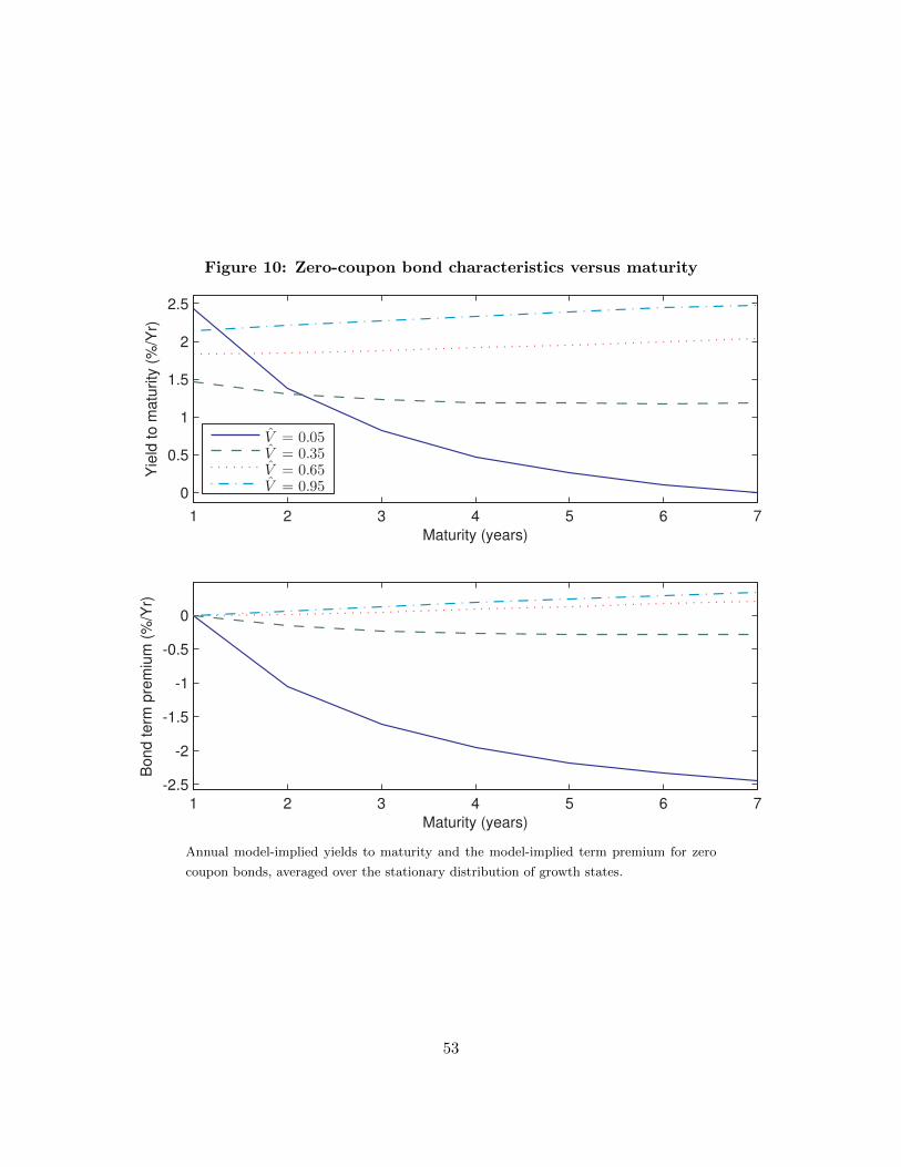
Figure 10: Zero-coupon bond characteristics versus maturity

1 2 3 4 5 6 7

0

0.5

1

1.5

2

2.5

Maturity (years)

Yie

ld to m

atu

rity

(%

/Yr)

1 2 3 4 5 6 7

-2.5

-2

-1.5

-1

-0.5

0

Maturity (years)

Bond term

pre

miu

m (

%/Y

r)

V = 0.05

V = 0.35

V = 0.65

V = 0.95

Annual model-implied yields to maturity and the model-implied term premium for zero

coupon bonds, averaged over the stationary distribution of growth states.

53

Figure 11: Portfolios

0.2 0.4 0.6 0.8

-1

0

1

2

3

4

x 104

Ag

en

t 1

V

0.2 0.4 0.6 0.8

-1

0

1

2

3

4

x 104

Ag

en

t 2

V

C

B1

F1

F2

Portfolios for each agent, in terms of numeraire value of investment in each asset, versus

V . Plots are averages over growth states using the stationary distribution.

Figure 12: Open interest in oil futures and spot prices

0.2 0.4 0.6 0.8

0

2

4

6

8

10

12

14

op

en

in

tere

st

(10

00

s)

V

0.2 0.4 0.6 0.840

50

60

70

80

sp

ot

price

V

F1

F2

The left panel shows model-implied open interest in 1 and 2 year oil futures contracts,

expressed as the numeraire value of the contracts in 1000s, versus agent two promised

utility V . The right panel shows spot price of oil versus V . Results are averaged over the

stationary distribution of growth states s.

54

Figure 13: Evolution over time

0 5 10 15 20 25 30 35 40 45

0.06

0.08

0.1

0.12

V

0 5 10 15 20 25 30 35 40 45

50

60

70

Sp

ot

price

0 5 10 15 20 25 30 35 40 45

5

10

15

20

25

Op

en

in

tere

st

(10

00

s)

0 5 10 15 20 25 30 35 40 45

0.12

0.14

0.16

0.18

0.2

0.22

0.24

No

rm.

op

en

in

tere

st

0 5 10 15 20 25 30 35 40 45

1.4

1.6

1.8

2

Fu

t. r

isk p

rem

ium

(%

)

Average path of the model economy over a 50-year period, conditional initial V0 = 0.05.

The initial growth state is selected according to the stationary distribution. From top to

bottom, the panels show V (indicative of agent two’s wealth share), the oil spot price,

open interest on 1-year futures, open interest normalized by aggregate wealth, and the

risk premium on one-year oil futures. Results are computed using Monte Carlo simulation

with 10000 paths.

55