Randomization Tests and Multi-Level Data in State Politics

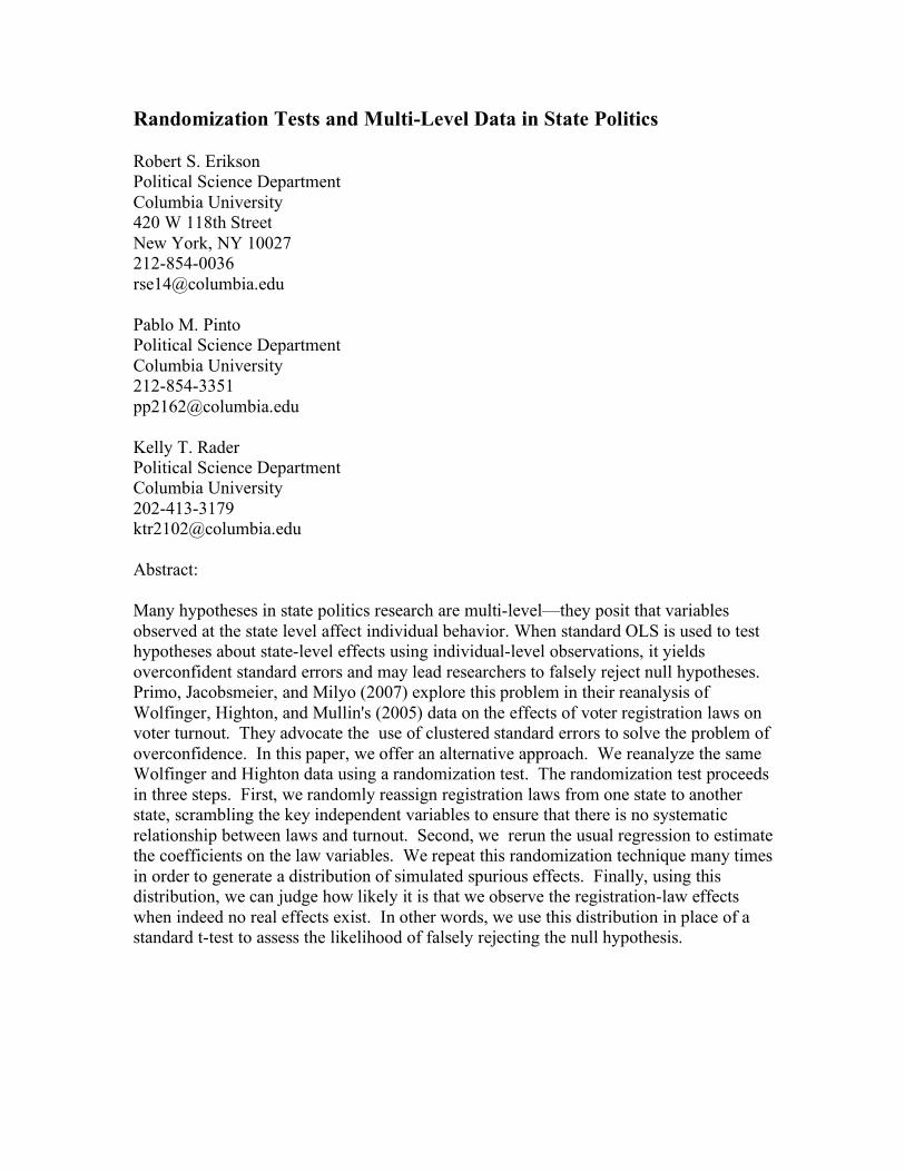
Randomization Tests and Multi-Level Data in State Politics

Robert S. Erikson

Political Science Department

Columbia University

420 W 118th Street

New York, NY 10027

212-854-0036

[email protected]

Pablo M. Pinto


Columbia University

212-854-3351

[email protected]

Kelly T. Rader


Columbia University

202-413-3179

[email protected]

Abstract:

Many hypotheses in state politics research are multi-level—they posit that variables

observed at the state level affect individual behavior. When standard OLS is used to test

hypotheses about state-level effects using individual-level observations, it yields

overconfident standard errors and may lead researchers to falsely reject null hypotheses.

Primo, Jacobsmeier, and Milyo (2007) explore this problem in their reanalysis of

Wolfinger, Highton, and Mullin's (2005) data on the effects of voter registration laws on

voter turnout. They advocate the use of clustered standard errors to solve the problem of

overconfidence. In this paper, we offer an alternative approach. We reanalyze the same

Wolfinger and Highton data using a randomization test. The randomization test proceeds

in three steps. First, we randomly reassign registration laws from one state to another

state, scrambling the key independent variables to ensure that there is no systematic

relationship between laws and turnout. Second, we rerun the usual regression to estimate

the coefficients on the law variables. We repeat this randomization technique many times

in order to generate a distribution of simulated spurious effects. Finally, using this

distribution, we can judge how likely it is that we observe the registration-law effects

when indeed no real effects exist. In other words, we use this distribution in place of a

standard t-test to assess the likelihood of falsely rejecting the null hypothesis.

1

Do various state-level reforms induce greater turnout at the polls in the US?

While some literature on this topic is time-serial in design, much of the reported evidence

is cross-sectional in nature. A decided limitation for cross-sectional analysis would seem

to be the limiting N of 50 cases when the states are the units of analysis. Cross-sectional

analysis seemingly undergoes a great improvement when the unit of analysis shifts to the

individual voter. Beginning with Wolfinger and Rosenstone (1980), many studies exploit

the US Census’s biennial post-election surveys of voter participation with its multiple

thousands of respondents. With 40,000 cases or more rather than a mere 50, the

advantage of using CPS survey data would seem would seem to be considerable. The

gain is not only in the number of cases but also in estimating effects at the state level

while controlling for effects at the individual level that would otherwise add noise to the

model.

As a recent example, we discuss the analysis by Wolfinger, Highton and Mullin

(2007)—hereafter WHM—of the effects of laws concerning post-registration aspects of

the costs of voting on the probability that a registered voter will turn out to vote.

According to this analysis, reforms such as early voting hours, late polling hours, and

many more innovations serve to boost turnout. As we will see, however, the claim is in

dispute. The challenge is the multi-level nature of the problem. The independent

variables of interest or treatments are administered at the state level. The responses are

by individual potential voters.

A troublesome aspect of this multi-level modeling is the accurate portrayal of the

standard errors of the law effects. When they are estimated via OLS, the standard errors

are deflated (and the significance inflated) in that the effective N for the state effects is

2

still 50 rather than the number of individual cases. The classic statement is by Moulton

(1986, 1990). See also Donald and Lang (2007) and Arceneaux and Nickerson (2007),

who present the general argument regarding how this problem applies to multi-level data.

Primo, Jacobsmeier, and Milyo (2007)—hereafter PJM—offer a useful illustration when

applied to Wolfinger, et al.’s analysis of state laws affecting voting among registrants.

As PJM show, when the standard errors for the state laws are correctly estimated, the

coefficients for the various state laws are mainly outside the range of statistical

significance. Thus it would seem that the evidence is actually rather unsettled whether

reform legislation actually boosts turnout among the registered.

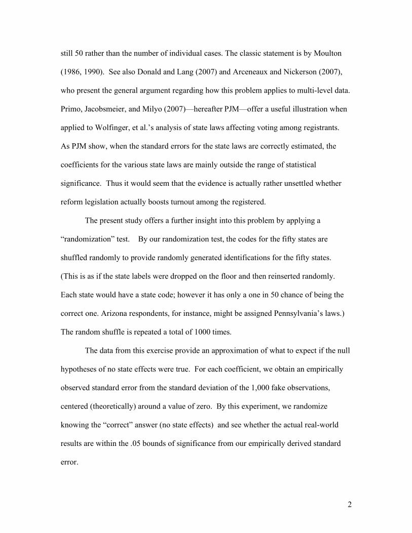
The present study offers a further insight into this problem by applying a

“randomization” test. By our randomization test, the codes for the fifty states are

shuffled randomly to provide randomly generated identifications for the fifty states.

(This is as if the state labels were dropped on the floor and then reinserted randomly.

Each state would have a state code; however it has only a one in 50 chance of being the

correct one. Arizona respondents, for instance, might be assigned Pennsylvania’s laws.)

The random shuffle is repeated a total of 1000 times.

The data from this exercise provide an approximation of what to expect if the null

hypotheses of no state effects were true. For each coefficient, we obtain an empirically

observed standard error from the standard deviation of the 1,000 fake observations,

centered (theoretically) around a value of zero. By this experiment, we randomize

knowing the “correct” answer (no state effects) and see whether the actual real-world

results are within the .05 bounds of significance from our empirically derived standard

error.

3

This test is particularly useful where the theoretical standard error is not easily

derived. While PJM estimate the appropriate clustered standard errors for the state-level

additive effects, it is not clear that the clustering option helps when it comes to interaction

effects between state-level (law) and individual level (e.g., education, age) variables.

With PJM’s clustering, these interactions remain “significant” and far more significant

than their state-level components. This is clearly wrong. But the theoretical remedy is

not clear. The randomization test however supplies a solution. Rather than a theoretical

derivation based on assumptions, it is empirically derived.

The Research Question

WHM (2005) use individual-level data from the 2000 Voter Supplement of the

Current Population Survey to test the effects of state postregistration laws on the

likelihood of turnout among individuals who are registered to vote. While turnout among

registered individuals is already relatively high, averaging 86 percent in their sample,

WHM hypothesize that certain state laws further decrease the cost of voting, even for

those who are already registered. Extended voting hours in the morning and evening,

time off from work on election day for public and private employees, and receipt of

sample ballots and polling place information in the mail give potential voters more time

and information. These laws, then, should be associated with higher turnout.

WHM also hypothesize that the effects of certain postregistration laws should

vary across different subgroups. For example, time off work for public employees should

primarily affect the likelihood that public employees will vote, as opposed to private

employees or the unemployed. Receiving sample ballots in the mail should primarily

affect the voting likelihood of individuals who do not already have the information, like

4

young and less educated people. To accommodate these potential across-group

differences, WHM set up a model with several interaction effects between individual

characteristics and state laws. Their specification is shown in Table 1.1

We do not object to the theory behind WHM’s hypotheses about the effects of

state postregistration laws on individual turnout. However, like PJM, we have concerns

about the precision with which those effects can be estimated given the multi-level

structure of the data. As PJM argue, the WHM data is generated by a process that

includes a compound error term. One part of the error is at the individual level, and one

part is at the state level. The state-level component induces clustering among

respondents in the same state. Standard regression techniques, like that employed by

WHM, ignore the state-level error component, and so they overstate the confidence with

which they estimate the effects of state-level variables.

There are several ways to deal with this compound error term. Strategies include

using clustered standard errors, modeling state random effects, employing a full

hierarchical linear model, and using OLS on data aggregated to the state level.

Arceneaux and Nickerson (2007) show that under the “ideal conditions” of random

treatment assignment and normally-distributed cluster-level and individual-level

disturbances, each of these techniques perform equally well. However, in the case of

observational data on turnout, they caution the choice is not so clear-cut. Estimated

standard errors and, in some cases, point estimates vary across models and are sensitive

to the assumptions imposed by each technique. For the WHM data, PJM advocate the

1 Because our focus is on the modeling of state-level characteristics and their interactions

with individual-level characteristics, we omit the individual characteristics in the WHM

model from our table. They include measures of employment status, education, age,

income, race, and residential stability.

5

use of clustered standard errors over hierarchical linear modeling because, theoretically,

clustering makes fewer assumptions, and, practically, clustering is easier to implement

with available software.

We argue that a randomization test might be useful in assessing multi-level

hypotheses like those in WHM, particularly those with multi-level interaction effects,

because, unlike the other methods, they do not rely on any distributional assumptions

about the disturbances in the model.

The randomization design

Randomization or permutation tests are a non-parametric way to derive standard

errors and significance tests for the effect of a variable on an outcome. They are used

widely in biology (e.g. Manly 1997) and increasingly in economics and business

applications (e.g. Kennedy and Cade 1996).

Typically we want to know how likely it is that an estimated coefficient is

different from the null hypothesis, usually zero. Standard parametric methods use some

function of the coefficient and the estimated standard errors to calculate a test statistic

that is theoretically distributed in some way and compare that test statistic to its reference

distribution. If that test statistic is relatively rare, then we can be confident that the

estimated coefficient is different from the null hypothesis. For example, in the simple

case of OLS, we estimate standard errors with the assumption that disturbances are

distributed i.i.d. N(0, !2). We derive a t-test statistic by taking the ratio of the estimated

coefficient and the estimated standard error and compare that statistic to a student’s t

distribution. If it is larger than the critical value 1.96 or smaller than -1.96 (for sample

6

sizes 1000 or larger), we reject the null hypothesis of no effect with 95 percent

confidence.

Randomization tests proceed in an analogous way but without relying on

theoretical distributions. First, we estimate the coefficient on a variable of interest and its

associated test statistic using our preferred model specification. Then, we randomly

reshuffle the data in such a way that we know there is no systematic relationship between

the variable and the observed outcome. Then, we re-run our preferred model on the

shuffled data and get a new estimate of the coefficient and test statistic. We reshuffle and

re-estimate a total of 1000 times. This process gives us a distribution of 1000 estimated

coefficients and 1000 test statistics centered, theoretically, at zero. This is the reference

distribution for the randomization test. By locating the observed effect (the estimated test

statistic) on this distribution we are able to assess the probability that effect could have

occurred by “chance.”

There are several ways to reshuffle data to break the relationship between a

variable of interest X1 and an outcome Y for a multivariate model with many covariates.

Kennedy (1995) reviews the most common methods in the literature. These include

simply shuffling X1 or shuffling Y. More complicated methods include “residualizing

Y”—residualizing Y with respect to the other covariates, shuffling the residualized Y,

and regressing it on X1—and “shuffling residuals”—regressing Y on the other covariates,

shuffling the residuals from this regression, adding them to the predicted Y from this

regression, and regressing the new Y vector on the other covariates and X1.

The results from Monte Carlo analyses in Kennedy and Cade (1996) suggest that

the simple method of shuffling X1 is sufficient in the multivariate context so long as

7

inferences are based on the distribution of test statistics and not on the distribution of

coefficients.2

Randomization tests were originally developed by Fisher (1935) to test the effect

of a treatment in a randomized experiment. Because experiments typically have smaller

sample sizes, it is possible to shuffle the data to represent all of the possible permutations

of treatment to subject. Then, the randomization test will be exact. However, in many

observational contexts, obtaining an exact randomization test is practically infeasible.

Sampling many times from the set of possible permutations gives an approximate

randomization test. Manly (1997) argues that, for 95 percent confidence levels,

randomization tests using 1000 draws should be powerful enough to detect an effect.

Unlike parametric significance tests, randomization tests make no assumptions

about the distribution of disturbances in a model and do not require the distribution of the

test statistics to be known. Thus, randomization tests are particularly useful in models

with complicated error structures for which theoretical standard errors are hard to derive.

However, randomization tests do make one important assumption about the

disturbances—that they are exchangeable. Exchangeability means that if the null

hypothesis is true, if the variable of interest indeed has no effect, then observed outcomes

across individuals would be similar (conditional on confounding covariates) no matter

2 The logic behind this recommendation is as follows. Shuffling X1 does not hold

constant the collinearity between X1 and the other covariates. Say, for example, that X1

and some other covariate X2 are highly collinear. Then, we would expect that the

standard errors on the coefficients of these variables to be large. Because shuffling X1

destroys the collinearity between X1 and X2, the coefficients obtained from the

randomization method may not vary as much as they would in actual repeated sampling.

Thus inferences from the distribution of randomized coefficients would be too confident.

Because test statistics are adjusted for variance magnitude, they are unaffected by

changing the collinearity in the data.

8

what the level of the variable of interest. In other words, if exchangeability holds, then

under the null hypothesis, the variable of interest is merely a label that can be applied to

any observation without changing the expected outcome. This justifies the shuffling

procedure.

Findings

To reassess the findings in WHM (2005), we performed a randomization test to

estimate empirically derived standard errors and test statistics for the coefficients in their

original model. First, we detached the state-level variables from the individual-level

observations. Then, we randomly reassigned state level-variables to state populations.

This particular randomization procedure preserves the menu of state laws and the

association of individuals within a state. For example, all of the residents of Georgia may

be randomly assigned all of the post-registration laws from Washington. It is possible

that the residents of Georgia may be randomly assigned the laws of Georgia and even that

we may recreate the actual dataset through random assignment. This is justified because,

under the null hypothesis, the actual data is considered to be equally likely as any other

permutation.

After shuffling the state laws, we recalculate the interaction terms between state-

level and individual-level effects. Finally, we rerun the WHM model and collect the

coefficients and z-values from standard significance tests. We repeat this process a total

of 1,000 times.

Table 1 replicates the multivariate logit model of turnout in WHM, with

unadjusted and clustered standard errors, and shows the estimated standard errors from

our randomization method. The randomized standard errors are more similar in size to

9

the clustered standard errors than to the unadjusted standard errors, though they are larger

than both. The only state law effect that retains significance is the incorrectly-signed

time off work for private employees. The interaction effects between mailed polling

place information and education, mailed sample ballots and education, and mailed sample

ballots and young living without parents are significant using clustered standard errors

but lose their significance with randomized standard errors.

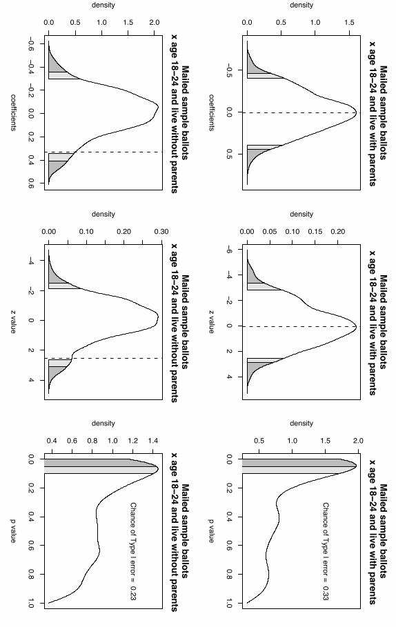
In Figure 1 (on pages 20-27), we display the results from our randomization test

in greater detail. We take the case of the possible effect of early voting hours as our

example for discussion. The relevant graphs for early voting hours are presented in the

top row. The first graph shows the density of the 1000 estimated coefficients on the early

voting hours indicator estimated using 1000 datasets in which we know there is no

systematic relationship between early voting hours and turnout. The distribution is, as

expected, centered around zero. The dark gray shaded area represents the 5 percent most

extreme coefficients, and the entire shaded area covers the 10 percent most extreme

coefficients. The dotted line indicates the magnitude of the coefficient estimated using

the actual observed data, the coefficient in Table 1. From this graph, we can see that the

estimated early voting hours effect is not rare by conventional statistical standards. It

does not fall among the 10 percent most extreme coefficients. Therefore, we cannot rule

out the possibility that the effect of early voting hours in the WHM model is just random

noise. We cannot reject the null hypothesis that the early voting hours effect on turnout

is zero. Again, the only state law effect that falls among the 10 percent most extreme in

its randomized distribution is the incorrectly signed time off work for private employees.

10

The second early voting hours graph in Figure 1 shows the density of the 1000 z-

values calculated using the conventional test of significance in a multivariate logit model

on the early voting hours effect. As in the coefficient graph, we see that the test statistic

derived from the actual data is not among the 10 percent most extreme. For all of the

state laws and interaction effects, the inferences drawn from the distribution of z values is

the same as that drawn from the distribution of coefficients.3

The third graph across the top of Figure 1 shows the distribution of 1000 p-values

associated with the 1000 coefficients, calculated using the conventional significance test.

The shaded area covers p-values that are 0.1 or smaller, small enough to justify rejecting

the null hypothesis that early voting hours have no effect on turnout. Even though these

p-values were calculated using data in which we know there is no systematic relationship

between laws and turnout, 66 percent of the p-values were less than or equal to 0.1. This

means that using standard significance tests with this data would cause one to falsely

infer that early voting hours have an effect on turnout 66 percent of the time, instead of

10 percent of the time, as we would expect at the 90 percent confidence level. Standard

tests on almost all of the post-registration laws exhibit higher than expected type I errors.

This underscores the importance of accounting for the clustered nature of the data.

Additive Models

As an alternative to the complexity of the model with interaction effects involving

respondents and states, we can estimate strictly additive models for subgroups who might

be particularly sensitive to the stimuli of reforms designed to induce voting among the

registered. Table 2 shows the results for 2 additive equations. The top equation is for all

3 This is probably because we shuffle the menu of state laws, instead of each laws

individually, which preserves the collinearity among the laws.

11

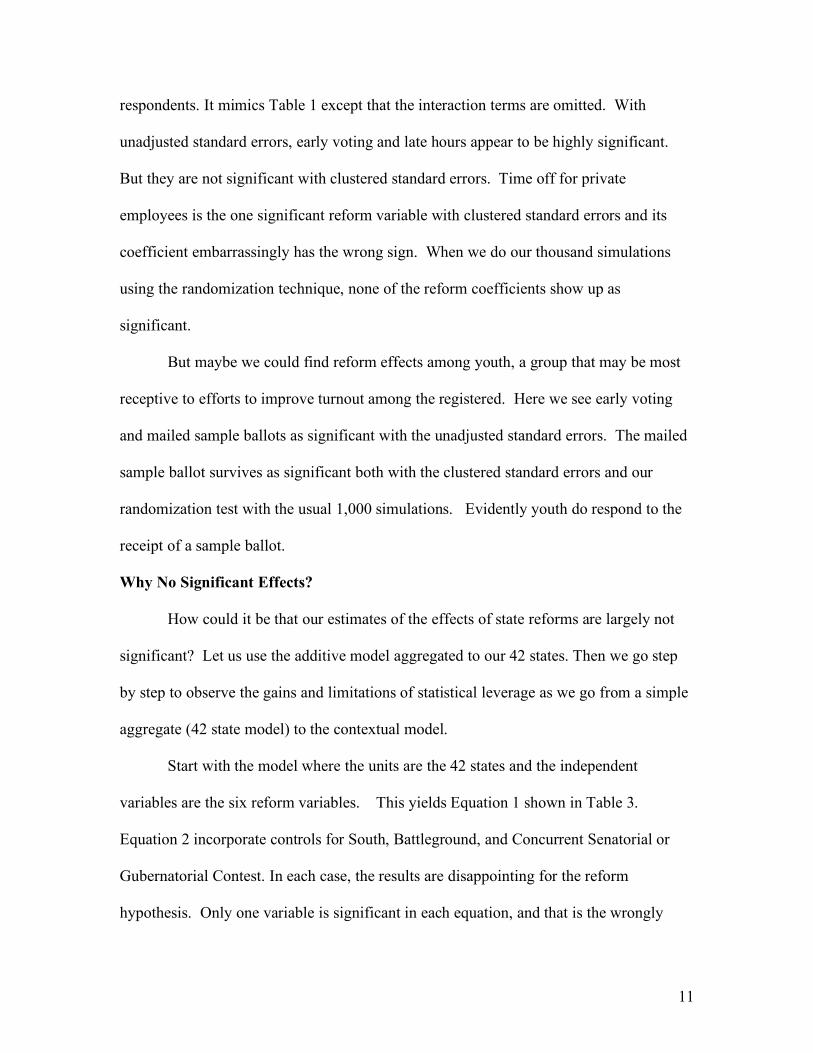
respondents. It mimics Table 1 except that the interaction terms are omitted. With

unadjusted standard errors, early voting and late hours appear to be highly significant.

But they are not significant with clustered standard errors. Time off for private

employees is the one significant reform variable with clustered standard errors and its

coefficient embarrassingly has the wrong sign. When we do our thousand simulations

using the randomization technique, none of the reform coefficients show up as

significant.

But maybe we could find reform effects among youth, a group that may be most

receptive to efforts to improve turnout among the registered. Here we see early voting

and mailed sample ballots as significant with the unadjusted standard errors. The mailed

sample ballot survives as significant both with the clustered standard errors and our

randomization test with the usual 1,000 simulations. Evidently youth do respond to the

receipt of a sample ballot.

Why No Significant Effects?

How could it be that our estimates of the effects of state reforms are largely not

significant? Let us use the additive model aggregated to our 42 states. Then we go step

by step to observe the gains and limitations of statistical leverage as we go from a simple

aggregate (42 state model) to the contextual model.

Start with the model where the units are the 42 states and the independent

variables are the six reform variables. This yields Equation 1 shown in Table 3.

Equation 2 incorporate controls for South, Battleground, and Concurrent Senatorial or

Gubernatorial Contest. In each case, the results are disappointing for the reform

hypothesis. Only one variable is significant in each equation, and that is the wrongly

12

signed coefficient for time off for private employees. Extended evening hours is barely

significant, but only without the added controls. Collectively, the six reforms have a

significance level of only .07 (.08 with the controls), short of the usual .05 benchmark.

The lesson from this barebones model is that we should want to control for

individual effects. Suppose we do so by adding a summary measure of the state-

aggregated individual effects from the individual-level equation. For this variable, we

take the prediction equation from the individual-level analysis and subtract out the

estimated effects of the state-level variables. Then we take the state means of this

individual-level equation and enter them into the state-level equation. The results are

shown in Equation 3.

We now have a summary control for the contribution of individual-level effects to

state turnout. Adding this variable allows us to explain half (but only half) of the

variance in state turnout. The important point is that with these controls the reform

coefficients are no more impressive than before. The control for state-level individual

effects generates some churning of the estimates, but they are decidedly not very

significant. Only time off for public employees passes the .05 threshold, but is almost

offset by the wrongly signed negative coefficient for time off for private employees.

With the added controls, the net effects of the six reforms become even less significant.

Controlling for state characteristics plus the individual-level characteristics of the state

samples, the six reforms are significant only at the .11 level.

While this exercise is informative, it is best to estimate the effects of the specific

reforms from the individual-level equation. From the individual-level equation we can

aggregate up to the state level in terms of the individual-specific characteristics, the state

13

characteristics, and the state reforms. For this exercise, we divide the individual-level

prediction equation into three components—the individual-level characteristics, the state-

level traits (South, Battleground, Sengov), and the important component based on the six

reforms. The results are shown in Table 4.

Here we see that all three sets of predictors are significant when aggregated to the

42 states. Of special interest is that the six predictors are collectively significant at the

.05 level. This may be the best we can do in terms of arguing for the collective

significance of the reforms on voting rates among registrants using the 2000 CPS data.

So, again, why cannot we do better at finding evidence that reforms boost

turnout? One’s intuition might be that once we know a state citizenry’s individual

characteristics and some state characteristics in terms of whether or not the state is

southern, a battleground state, or has a senatorial or gubernatorial contest that we can

explain most of the factors affecting a state’s turnout. It would seem then that with little

further residual variation to control for, we can readily estimate the effects of reforms on

turnout. But our surmise is incorrect. Combining individual characteristics (as

measured), state characteristics, plus our reforms, we can do no more than explain half

the variance of turnout among registrants in the 42 states. With turnout reforms leading

to modest effects at best, it is no wonder that the reform coefficients are rarely significant

Conclusions

We have used the nonparametric technique known as the randomization design to

show that the reported effects of reforms designed to encourage turnout among registered

voters are not statistically significant. Specifically, we conducted multiple simulations

14

where the state labels were scrambled so that the distributions of the clusters of laws were

assigned randomly. Alabama might get Minnesota’s laws, etc.

We applied this methodology both to the WHM interactive model and to the

additive version. We also applied the additive version to a youth sample. Based on the

simulations, the observed coefficients for state laws from the WHM analysis of turnout

effects are essentially not statistically significant. The WHM model is of individual

voters, with state-level variables as contextual variables. Two alternatives are to employ

multilevel modeling (with random effects) and to employ fixed effects where state

dummy variable coefficients from the individual analysis are modeled in terms of state

characteristics. We anticipate that randomization tests for these models would also

suggest reform effects outside the .usual bounds of significance.

The data for this study is from a cross-section of registered voters in 2000. As a

cross-sectional study, the analysis is limited by endogeneity concerns. Reforms are not

distributed randomly in the states. We might expect that states with high turnout levels

are most prone to pass legislation that expedites the voting process. Alternatively, it

might be that state legislatures are more likely to pass legislation as a response to a

sluggish voting record. These possibilities are reason why the best design for inferring

the effects of reform legislation would be some sort of a time series design.

Despite the “negative” nature of our findings, we do not argue that legislation

designed to encourage turnout among registered voters is ineffectual. The various acts

such as early voting and late hours may well have their intended intent. There is nothing

in our findings that would deny that reforms influence turnout by at least a few

percentage points. But if their effects are to push turnout up by only a few percentage

15

points, the effects are not easy to estimate at the state level. There is sufficient noise in

the form of unobserved sources of state turnout to prevent the estimated effects to pass

the usual thresholds of statistical significance.

References

Arceneaux, Kevin and David W. Nickerson. 2007. “Correctly Modeling Certainty with

Clustered Treatments: A Comparison of Methods.” Unpublished paper.

Donald, Stephen G. and Kevin Lang. 2007. “Inference with Difference-in-Differences

and Other Panel Data.” Review of Economics and Statistics. 89: 221-233.

Fisher, R.A. 1935. The Design of Experiments. Edinburgh: Oliver and Boyd.

Kennedy, Peter E. 1995. “Randomization Tests in Econometrics.” Journal of Business

and Economic Statistics. 13: 85-94.

Kennedy, Peter E., and Brian S. Cade. 1996. “Randomizaion Tests for Multiple

Regression.” Communications in Statistics – Simulation and Computation. 34: 923-936.

Manly, Bryan F. J. 1997. Randomization, Bootstrap and Monte Carlo Methods in

Biology. London, Chapman Hall. 2nd

ed.

Moulton, Brent R. 1986. “Random Group Effects and the Precision of Regression

Estimates.” Journal of Econometrics. 32: 385-397.

Moulton, Brent R. 1990. “An Illustration of a Pitfall in Estimating the Effects of

Aggregate Variables in Micro Units.” Review of Economics and Statistics. 72: 334-338.

Primo, David M., Matthew I. Jacobsmeier, and Jefrey Milyo. 2007. “Estimating the

Impact of State Policies and Institutions with Mixed-Level Data.” State Politics and

Policy Quarterly. 7: 446-459.

Wolfinger, Raymond E., Benjamin Highton, and Megan Mullin. 2005. “How

Postregistration Laws Affect the Turnout of Citizens Registered to Vote.” State Politics

and Policy Quarterly. 5: 1-23.

Wolfinger, Ramond E. and Steven J. Rosenstone. 1980. Who Votes? New Haven: Yale

University Press.

16

Table 1: Comparison of Standard Errors in Full Turnout

Model

Full Model

Coefficient

Unadjusted

Standard

Errors

Clustered

Standard

Errors

Randomized

Standard Errors

Early voting 0.14 0.03 *** 0.10 0.12

Late voting 0.08 0.04 ** 0.08 0.11

Mailed polling place information 0.24 0.12 ** 0.22 0.25

Mailed polling place information x

education -0.08 0.04 ** 0.04 * 0.07

Mailed sample ballots 0.29 0.12 ** 0.18 0.27

Mailed sample ballots x education -0.09 0.04 ** 0.04 ** 0.08

Mailed sample ballots x age 18--24 and

live with parents 0.01 0.12 0.28 0.24

Mailed sample ballots x age 18--24 and

live without parents 0.33 0.13 ** 0.16 ** 0.19

Time off work for state employees 0.06 0.05 0.10 0.15

Time off work for state employees x state

employee -0.02 0.19 0.16 0.17

Time off work for private employees -0.19 0.05 *** 0.07 *** 0.12 *

Time off work for private employees x

private employee 0.03 0.06 0.05 0.06

Southern state -0.19 0.04 *** 0.08 ** 0.13

Battleground state 0.08 0.03 ** 0.07 0.11

Concurent senatorial or gubernatorial

contest -0.09 0.04 ** 0.08 0.13

N=44,859

*p<.10; **p<.05; ***p<.01; N=44,859

17

Table 2. Additive Models for All Respondents and for Youth, 18-24 only

Additive Model, All

Respondents Coefficient

Unadjusted

Standard

Errors

Clustered

Standard

Errors

Randomization

Standard

Errors

Early voting 0.14 0.03 *** 0.10 0.11

Late voting 0.08 0.04 ** 0.08 0.11

Mailed polling place

information 0.04 0.06 0.14 0.16

Mailed sample ballots 0.09 0.05 0.12 0.16

Time off work for state

employees 0.06 0.05 0.10 0.15

Time off work for private

employees -0.18 0.04 *** 0.06 *** 0.13

Southern state -0.19 0.04 *** 0.08 ** 0.12

Battleground state 0.08 0.03 * 0.07 0.11

Concurrent senatorial or

gubernatorial contest -0.09 0.04 * 0.08 0.13

N=44,859

*p<.10; **p<.05; ***p<.01

Additive model, 18-24 only

Coefficient

Unadjusted

Standard

Errors

Clustered Standard

Errors

Randomization

Standard

Errors

Early voting 0.20 0.09 ** 0.13 0.16

Late voting 0.12 0.09 0.12 0.15


information -0.15 0.15 0.19 0.21

Mailed sample ballots 0.49 0.13 *** 0.20 ** 0.22 *

Time off work for state

employees -0.16 0.12 0.15 0.21

Time off work for private

employees 0.06 0.10 0.13 0.18

Southern state -0.06 0.10 0.10 0.18

Battleground state -0.01 0.09 0.11 0.15

Concurrent senatorial or

gubernatorial contest -0.30 0.10 *** 0.10 *** 0.18 *

N=3,697

*p<.10; **p<.05; ***p<.01;

Individual-level variables are omitted..

18

Table 3. Aggregate Analyses Using States as Units

Equation 1 Equation 2 Equation 3

Coefficient

Standard

Errors

Coefficient

Standard

Errors

Coefficient

Standard

Errors

Early voting 0.17 0.08 * 0.06 0.09 0.00 0.09

Late voting 0.04 0.13 0.13 0.09 0.10 0.09


information 0.01 0.04 -0.03 0.13 0.00 0.13

Mailed sample ballots 0.19 0.12 0.03 0.04 -0.02 0.04

Time off work for

state employees -0.23 0.10 * 0.15 0.12 0.22 0.12 *

Time off work for

private employees 0.17 0.08 * -0.27 0.10 * -0.16 0.10

Southern state -0.22 0.10 * 0.56 0.18 **


Concurrent senatorial

or gubernatorial

contest

-0.03 0.10 0.26 0.10 *

Mean individual

predicting from

respondent

characteristics

1.74 0.36 ***

Adjusted R squared 0.14 0.19 0.52

Probability the 6

reforms are

collectively significant .07

.08

.11

N=42

*p<.05; **p<.01; ***p<.001

Table 3. Aggregate Analyses Using States as Units

Equation 1 Equation 2 Equation 3

Coefficient

Standard

Errors

Coefficient

Standard

Errors

Coefficient

Standard

Errors

Early voting 0.17 0.08 * 0.06 0.09 0.00 0.09

Late voting 0.04 0.13 0.13 0.09 0.10 0.09


information 0.01 0.04 -0.03 0.13 0.00 0.13

Mailed sample ballots 0.19 0.12 0.03 0.04 -0.02 0.04

Time off work for

state employees -0.23 0.10 * 0.15 0.12 0.22 0.12 *

Time off work for

private employees 0.17 0.08 * -0.27 0.10 * -0.16 0.10

Southern state -0.22 0.10 * 0.56 0.18 **


Concurrent senatorial

or gubernatorial

contest

-0.03 0.10 0.26 0.10 *

Mean individual

predicting from

respondent

characteristics

1.74 0.36 ***

Adjusted R squared 0.14 0.19 0.52

Probability the 6

reforms are

collectively significant .07

.08

.11

N=42

*p<.05; **p<.01; ***p<.001

19

Table 4 Predicting State Level Turnout from Three Components

Coefficient Standard

Error

Individual Level Predictions 1.20 0.29 ***

State Characteristics 1.50 0.68 *

State Level Reforms 0.63 0.31 *

N=42

Adjusted R squared = 0.49

*p<.05; **p<.01; ***p<.001

−0.4−0.2

0.00.2

0.4

0.0 0.5 1.0 1.5 2.0 2.5 3.0Early voting

coefficients

density

−10−5

05

10

0.00 0.04 0.08

Early voting

z value

density

0.00.2

0.40.6

0.81.0

1 2 3 4 5

Early voting

p value

density

Chance of Type I error = 0.66

−0.4−0.2

0.00.2

0.4

0.0 0.5 1.0 1.5 2.0 2.5 3.0

Late voting

coefficients

density

−10−5

05

10

0.00 0.02 0.04 0.06 0.08 0.10

Late voting

z value

density

0.00.2

0.40.6

0.81.0

0 1 2 3 4 5 6

Late voting

p value

density


−0.50.0

0.51.0

0.0 0.5 1.0 1.5M

ailed polling place information

coefficients

density

−10−5

05

0.00 0.05 0.10 0.15

Mailed polling place inform

ation

z value

density

0.00.2

0.40.6

0.81.0

0.5 1.0 1.5 2.0 2.5


ation

p value

density


−0.2−0.1

0.00.1

0.2

0 1 2 3 4 5


ation x education

coefficients

density

−4−2

02

46

0.00 0.05 0.10 0.15 0.20


ation x education

z value

density

0.00.2

0.40.6

0.81.0

0.5 1.0 1.5


ation x education

p value

density


−1.0−0.5

0.00.5

1.0

0.0 0.4 0.8 1.2M

ailed sample ballots

coefficients

density

−50

5

0.00 0.05 0.10 0.15

Mailed sam

ple ballots

z value

density

0.00.2

0.40.6

0.81.0

0.5 1.0 1.5 2.0 2.5

Mailed sam

ple ballots

p value

density


−0.3−0.2

−0.10.0

0.10.2

0.3

0 1 2 3 4

Mailed sam

ple ballots x education

coefficients

density

−6−4

−20

24

6

0.00 0.05 0.10 0.15 0.20

Mailed sam


z value

density

0.00.2

0.40.6

0.81.0

0.5 1.0 1.5 2.0

Mailed sam


p value

density


−0.50.0

0.5

0.0 0.5 1.0 1.5M

ailed sample ballots

x age 18−24 and live with parents

coefficients

density

−6−4

−20

24

0.00 0.05 0.10 0.15 0.20

Mailed sam

ple ballots x age 18−24 and live w

ith parents

z value

density

0.00.2

0.40.6

0.81.0

0.5 1.0 1.5 2.0

Mailed sam


ith parents

p value

density


−0.6−0.4

−0.20.0

0.20.4

0.6

0.0 0.5 1.0 1.5 2.0

Mailed sam


ithout parents

coefficients

density

−4−2

02

4

0.00 0.10 0.20 0.30

Mailed sam


ithout parents

z value

density

0.00.2

0.40.6

0.81.0

0.4 0.6 0.8 1.0 1.2 1.4

Mailed sam


ithout parents

p value

density


−0.4−0.2

0.00.2

0.40.6

0.0 0.5 1.0 1.5 2.0Tim

e off work for state em

ployees

coefficients

density

−10−5

05

10

0.00 0.04 0.08

Time off w

ork for state employees

z value

density

0.00.2

0.40.6

0.81.0

0 1 2 3 4 5 6

Time off w


p value

density


−0.6−0.4

−0.20.0

0.20.4

0.6

0.0 0.5 1.0 1.5 2.0 2.5

Time off w


x state employee

coefficients

density

−3−2

−10

12

3

0.0 0.1 0.2 0.3 0.4 0.5

Time off w


x state employee

z value

density

0.00.2

0.40.6

0.81.0

0.4 0.6 0.8 1.0 1.2

Time off w


x state employee

p value

density


−0.4−0.2

0.00.2

0.4

0.0 0.5 1.0 1.5 2.0 2.5 3.0Tim

e off work for private em

ployees

coefficients

density

−50

5

0.00 0.05 0.10 0.15

Time off w

ork for private employees

z value

density

0.00.2

0.40.6

0.81.0

0.5 1.0 1.5 2.0 2.5 3.0

Time off w


p value

density


−0.2−0.1

0.00.1

0.2

0 1 2 3 4 5 6 7

Time off w


x private employee

coefficients

density

−4−2

02

4

0.0 0.1 0.2 0.3

Time off w


x private employee

z value

density

0.00.2

0.40.6

0.81.0

0.5 0.6 0.7 0.8 0.9 1.0 1.1

Time off w


x private employee

p value

density


−0.4−0.2

0.00.2

0.4

0.0 0.5 1.0 1.5 2.0 2.5 3.0Southern state

coefficients

density

−10−5

05

10

0.00 0.04 0.08 0.12

Southern state

z value

density

0.00.2

0.40.6

0.81.0

0 1 2 3 4 5

Southern state

p value

density


−0.4−0.2

0.00.2

0.0 0.5 1.0 1.5 2.0 2.5 3.0

Battleground state

coefficients

density

−10−5

05

10

0.00 0.02 0.04 0.06 0.08 0.10

Battleground state

z value

density

0.00.2

0.40.6

0.81.0

0 1 2 3 4 5 6

Battleground state

p value

density


−0.4−0.2

0.00.2

0.4

0.0 0.5 1.0 1.5 2.0 2.5 3.0Concurrent senatorial

or gubernatorial contest

coefficients

density

−10−5

05

10

0.00 0.04 0.08

Concurrent senatorial or gubernatorial contest

z value

density

0.00.2

0.40.6

0.81.0

0 1 2 3 4 5 6

Concurrent senatorial or gubernatorial contest

p value

density


Randomization Tests and Multi-Level Data in State Politics

Documents

Transcript of Randomization Tests and Multi-Level Data in State Politics