Math 141 - Lecture 17: Bootstrapping and Randomization...
32
Math 141 Lecture 17: Bootstrapping and Randomization tests Albyn Jones 1 1 Library 304 [email protected] www.people.reed.edu/∼jones/courses/141 Albyn Jones Math 141
Transcript of Math 141 - Lecture 17: Bootstrapping and Randomization...
Math 141Lecture 17: Bootstrapping and Randomization tests
Albyn Jones1
1Library [email protected]
www.people.reed.edu/∼jones/courses/141
Albyn Jones Math 141
Non-Normal data
Question: The t-test depends on having normally distributeddata. What do we do with data that are clearly non-normal, orwhen we have nonlinear functions of normally distributed data?
Albyn Jones Math 141
Non-Normal Data: Analysis Options
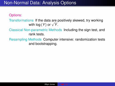
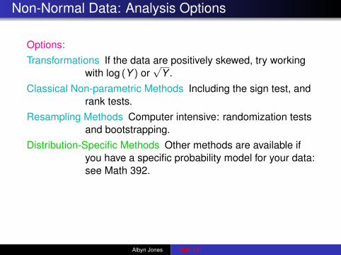
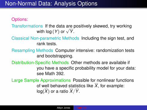
Options:
Transformations If the data are positively skewed, try workingwith log (Y ) or
√Y .
Classical Non-parametric Methods Including the sign test, andrank tests.
Resampling Methods Computer intensive: randomization testsand bootstrapping.
Distribution-Specific Methods Other methods are available ifyou have a specific probability model for your data:see Math 392.
Large Sample Approximations Possible for nonlinear functionsof well behaved statistics like X , for example:log(X ) or a ratio X/Y .
Albyn Jones Math 141
Non-Normal Data: Analysis Options
Options:Transformations If the data are positively skewed, try working
with log (Y ) or√
Y .
Classical Non-parametric Methods Including the sign test, andrank tests.
Resampling Methods Computer intensive: randomization testsand bootstrapping.
Distribution-Specific Methods Other methods are available ifyou have a specific probability model for your data:see Math 392.
Large Sample Approximations Possible for nonlinear functionsof well behaved statistics like X , for example:log(X ) or a ratio X/Y .
Albyn Jones Math 141
Non-Normal Data: Analysis Options
Options:Transformations If the data are positively skewed, try working
with log (Y ) or√
Y .Classical Non-parametric Methods Including the sign test, and
rank tests.
Resampling Methods Computer intensive: randomization testsand bootstrapping.
Distribution-Specific Methods Other methods are available ifyou have a specific probability model for your data:see Math 392.
Large Sample Approximations Possible for nonlinear functionsof well behaved statistics like X , for example:log(X ) or a ratio X/Y .
Albyn Jones Math 141
Non-Normal Data: Analysis Options
Options:Transformations If the data are positively skewed, try working
with log (Y ) or√
Y .Classical Non-parametric Methods Including the sign test, and
rank tests.Resampling Methods Computer intensive: randomization tests
and bootstrapping.
Distribution-Specific Methods Other methods are available ifyou have a specific probability model for your data:see Math 392.
Large Sample Approximations Possible for nonlinear functionsof well behaved statistics like X , for example:log(X ) or a ratio X/Y .
Albyn Jones Math 141
Non-Normal Data: Analysis Options
Options:Transformations If the data are positively skewed, try working
with log (Y ) or√
Y .Classical Non-parametric Methods Including the sign test, and
rank tests.Resampling Methods Computer intensive: randomization tests
and bootstrapping.Distribution-Specific Methods Other methods are available if
you have a specific probability model for your data:see Math 392.
Large Sample Approximations Possible for nonlinear functionsof well behaved statistics like X , for example:log(X ) or a ratio X/Y .
Albyn Jones Math 141
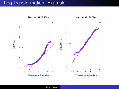
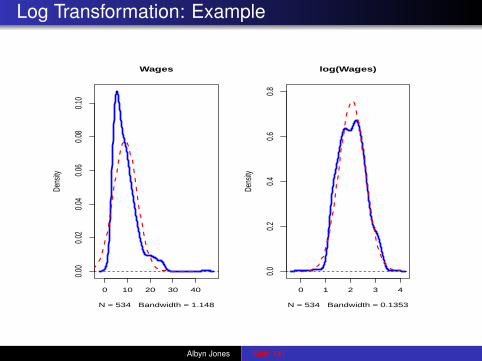
Transformations
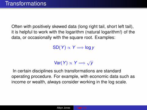
Often with positively skewed data (long right tail, short left tail),it is helpful to work with the logarithm (natural logarithm!) of thedata, or occasionally with the square root. Examples:
SD(Y ) ∝ Y =⇒ log y
Var(Y ) ∝ Y =⇒√
y
In certain disciplines such transformations are standardoperating procedure. For example, with economic data such asincome or wealth, always consider working in the log scale.
Albyn Jones Math 141
Log Transformation: Example
●
●
●
●
●
●●
●
●
●
●
●
●
●
●
●
●
●
●
●
●
●
●
●
●
●
●
●
●
●
●
●
●
●
●
●
●
●●
●
●
●
●
●
●
●
●
●
●
●
●
●
●●●
●
●
●
●
●
●
●
●
●
●
●
●
●
●
●
●
●
●
●
●
●
●
● ●
●
●
●
●
●●
●
●
●
●●
●●
●
●
●●
●
●
●
●
●
●
●●
●
●
●
●
●
●
●
●
●
●
●
●
●
●
●
●
●
●
●
●
●
●
●
●
●
●
●
●
●
●
●
●
●
●
●
●
●
●
●
●●
●
●
●
●
●
●●
●
●●
●
●
●
●
●
●
●
●
●
●
●
●
●
●
●
●●
●
●
●
●
●
●
●
●●
●
●
●
●
●
●
●
●
●
●
●
●
●
●●
●
●
●
●
●
●
●
●
●
●
●
●●●
●
●
●
●
●
●
●
●
●
●
●
●
●
●●
●
●
●●
●
●
●
●
●
●
●
●●●
●
●
●
●●
●
●
●
●
●
●
●
●
●
●
●
●●
●
●
●
●
●
●
●
●
●
●
●
●
●
●
●
●
●
●
●
●●
●
●
●
●
●●
●
●
●
●
●
●●
●
●
●●
●
●
●
●
●
●
●
●
●
●
●
●
●
●●
●
●
●
●
●
●
●
●
●●
●
●
●●
●
●
●
●
●
●
●
●
●
●
●●
●
●
●
●
●
●●
●●
●
●
●
●
●●
●
●
●
●●
●
●
●
●
●
●●
●
●
●●
●
●
●
●
●
●●●
●●
●
●
●●●
●
●
●
●
●
●
●
●
●
●
●
●
●●
●
●
●
●
●
●
●
●
●
●
●
●
●●
●
●●
●●●
●●
●
●
●●
●
●
●
●
●
●
●
●
●
●
●
●
●
●●
●●
●
●
●
●
●
●
●
●●●
●
●
●
●●
●
●
●
●
●
●
●
●
●
●
●
●
●
●●
●
●
●●
●
●
●
●
●
●
●
●
●
●
●●
●●
●
●
●●●
●
●
●
●
●
●
●
●●
●
●
●
●
●
●
●
●
●
●●
●
●
●●
●
●
●
●
●
●
●
●
●
●
●
●
●
●
●
●
●
●
−3 −2 −1 0 1 2 3
010
2030
40Normal Q−Q Plot
Theoretical Quantiles
CPS:
Wag
es ●
●
●
●
●
●●
●
●
●
●
●
●
●
●
●
●
●
●
●
●
●
●
●
●
●
●
●
●
●
●
●
●
●
●
●
●
●●
●
●
●
●
●
●
●
●
●
●
●
●
●
●
●●
●
●
●
●
●
●
●
●
●
●
●
●
●
●
●
●
●
●
●
●
●
●
● ●
●
●
●
●
●
●
●
●
●
●●
●●
●
●
●●
●
●
●
●●
●
●●
●
●
●
●
●
●
●
●
●
●
●
●
●
●
●
●
●
●
●
●
●
●
●
●
●
●
●
●
●
●
●
●
●
●
●
●
●
●
●
●●
●
●
●
●
●
●●
●
●●
●
●
●
●
●
●
●
●
●
●
●
●
●
●
●
●●
●
●
●
●
●
●
●
●
●
●
●
●
●
●
●
●
●
●
●
●
●
●
●●
●
●
●
●
●
●
●
●
●
●
●
●●●
●
●
●
●
●
●
●
●
●
●
●
●
●
●
●
●
●
●●
●
●
●
●
●
●
●
●●●
●●
●
●●
●
●
●
●
●
●
●
●
●
●
●
●●
●
●
●
●
●
●
●
●
●
●
●
●
●
●
●
●
●
●
●
●●
●
●
●
●
●●
●
●
●
●
●
●●
●
●
●
●
●
●
●
●
●
●
●
●
●
●
●
●
●
●●
●
●
●
●
●
●
●
●
●●
●
●
●●
●
●
●
●
●
●
●
●
●
●
●
●
●
●
●
●
●
●
●
●●
●
●
●
●
●●
●
●
●
●
●
●
●
●
●
●
●
●
●
●
●●
●
●
●
●
●
●●●
●●
●
●
●
●●
●
●
●
●
●
●
●
●
●
●
●
●
●
●
●
●
●
●
●
●
●
●
●
●
●
●
●●
●
●
●
●●
●
●●
●
●
●●
●
●
●
●
●
●●
●
●
●
●
●
●
●●
●●
●
●
●
●
●
●
●
●●●
●
●
●
●●
●
●
●
●
●
●
●
●
●
●
●
●
●
●
●
●
●
●
●
●
●
●
●
●
●
●
●
●
●
●
●
●●
●
●
●●●
●
●
●
●
●
●
●
●●
●
●
●
●
●
●
●
●
●
●
●
●
●
●
●
●
●
●
●
●
●
●
●
●
●
●
●
●
●
●
●
●
●
−3 −2 −1 0 1 2 3
01
23
Normal Q−Q Plot
Theoretical Quantiles
CPS:
log(W
ages
)
Albyn Jones Math 141
Log Transformation: Example
0 10 20 30 40
0.00
0.02
0.04
0.06
0.08
0.10
Wages
N = 534 Bandwidth = 1.148
Dens
ity
0 1 2 3 4
0.00.2
0.40.6
0.8
log(Wages)
N = 534 Bandwidth = 0.1353
Dens
ity
Albyn Jones Math 141
Sign Test and Rank Test
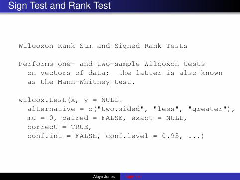
Wilcoxon Rank Sum and Signed Rank Tests
Performs one- and two-sample Wilcoxon testson vectors of data; the latter is also knownas the Mann-Whitney test.
wilcox.test(x, y = NULL,alternative = c("two.sided", "less", "greater"),mu = 0, paired = FALSE, exact = NULL,correct = TRUE,conf.int = FALSE, conf.level = 0.95, ...)
Albyn Jones Math 141
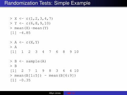
Randomization Tests
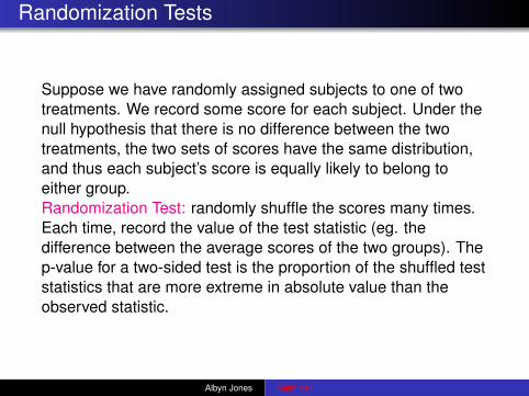
Suppose we have randomly assigned subjects to one of twotreatments. We record some score for each subject. Under thenull hypothesis that there is no difference between the twotreatments, the two sets of scores have the same distribution,and thus each subject’s score is equally likely to belong toeither group.Randomization Test: randomly shuffle the scores many times.Each time, record the value of the test statistic (eg. thedifference between the average scores of the two groups). Thep-value for a two-sided test is the proportion of the shuffled teststatistics that are more extreme in absolute value than theobserved statistic.
Albyn Jones Math 141
Randomization Tests: Simple Example
> X <- c(1,2,3,4,7)> Y <- c(6,8,9,10)> mean(X)-mean(Y)[1] -4.85
> A <- c(X,Y)> A[1] 1 2 3 4 7 6 8 9 10
> B <- sample(A)> B[1] 2 7 1 9 8 3 6 4 10> mean(B[1:5]) - mean(B[6:9])[1] -0.35
Albyn Jones Math 141
Randomization Tests: Example
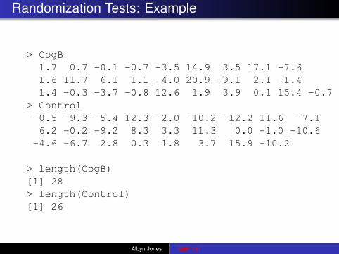
> CogB1.7 0.7 -0.1 -0.7 -3.5 14.9 3.5 17.1 -7.61.6 11.7 6.1 1.1 -4.0 20.9 -9.1 2.1 -1.41.4 -0.3 -3.7 -0.8 12.6 1.9 3.9 0.1 15.4 -0.7
> Control-0.5 -9.3 -5.4 12.3 -2.0 -10.2 -12.2 11.6 -7.16.2 -0.2 -9.2 8.3 3.3 11.3 0.0 -1.0 -10.6-4.6 -6.7 2.8 0.3 1.8 3.7 15.9 -10.2
> length(CogB)[1] 28> length(Control)[1] 26
Albyn Jones Math 141
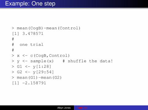
Example: One step
> mean(CogB)-mean(Control)[1] 3.478571## one trial#> x <- c(CogB,Control)> y <- sample(x) # shuffle the data!> G1 <- y[1:28]> G2 <- y[29:54]> mean(G1)-mean(G2)[1] -2.158791
Albyn Jones Math 141
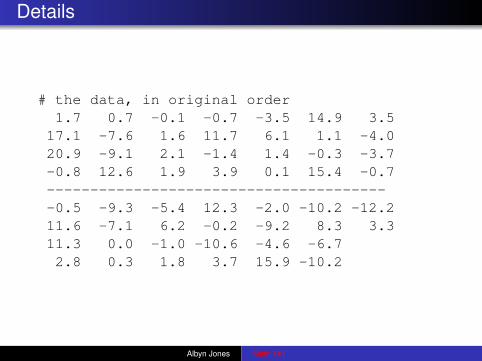
Details
# the data, in original order1.7 0.7 -0.1 -0.7 -3.5 14.9 3.517.1 -7.6 1.6 11.7 6.1 1.1 -4.020.9 -9.1 2.1 -1.4 1.4 -0.3 -3.7-0.8 12.6 1.9 3.9 0.1 15.4 -0.7----------------------------------------0.5 -9.3 -5.4 12.3 -2.0 -10.2 -12.211.6 -7.1 6.2 -0.2 -9.2 8.3 3.311.3 0.0 -1.0 -10.6 -4.6 -6.72.8 0.3 1.8 3.7 15.9 -10.2
Albyn Jones Math 141
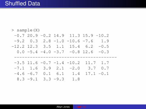
Shuffled Data
> sample(X)-0.7 20.9 -0.2 14.9 11.3 15.9 -10.2-9.2 0.3 2.8 -1.0 -10.6 -7.6 1.9
-12.2 12.3 3.5 1.1 15.4 6.2 -0.50.0 -5.4 -4.0 -3.7 -0.8 12.6 -0.3----------------------------------------3.5 11.6 -0.7 -1.4 -10.2 11.7 1.7-7.1 1.6 3.9 2.1 -2.0 3.7 0.7-4.6 -6.7 0.1 6.1 1.4 17.1 -0.18.3 -9.1 3.3 -9.3 1.8
Albyn Jones Math 141
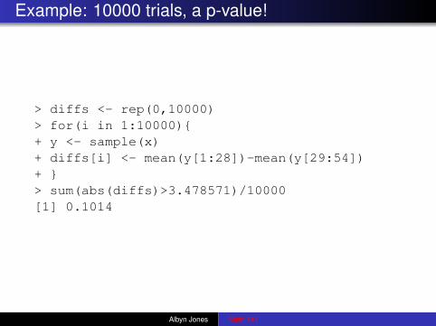
Example: 10000 trials, a p-value!
> diffs <- rep(0,10000)> for(i in 1:10000){+ y <- sample(x)+ diffs[i] <- mean(y[1:28])-mean(y[29:54])+ }> sum(abs(diffs)>3.478571)/10000[1] 0.1014
Albyn Jones Math 141
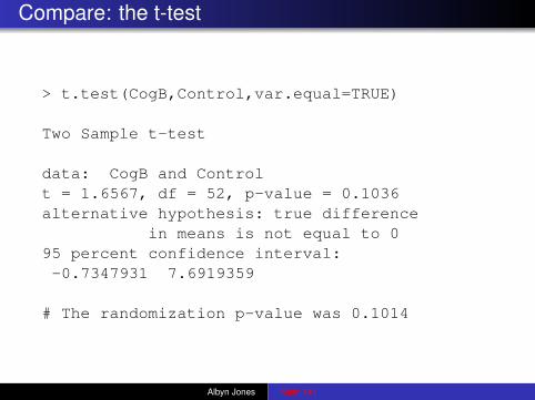
Compare: the t-test
> t.test(CogB,Control,var.equal=TRUE)
Two Sample t-test
data: CogB and Controlt = 1.6567, df = 52, p-value = 0.1036alternative hypothesis: true difference
in means is not equal to 095 percent confidence interval:-0.7347931 7.6919359
# The randomization p-value was 0.1014
Albyn Jones Math 141
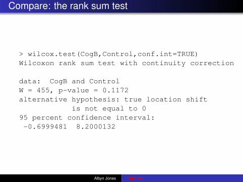
Compare: the rank sum test
> wilcox.test(CogB,Control,conf.int=TRUE)Wilcoxon rank sum test with continuity correction
data: CogB and ControlW = 455, p-value = 0.1172alternative hypothesis: true location shift
is not equal to 095 percent confidence interval:-0.6999481 8.2000132
Albyn Jones Math 141
Randomization test advantages
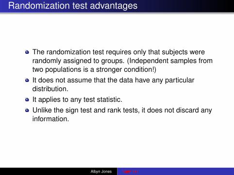
The randomization test requires only that subjects wererandomly assigned to groups. (Independent samples fromtwo populations is a stronger condition!)It does not assume that the data have any particulardistribution.It applies to any test statistic.Unlike the sign test and rank tests, it does not discard anyinformation.
Albyn Jones Math 141
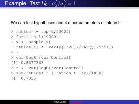
Example: Test H0 : σ2x/σ
2y = 1
We can test hypotheses about other parameters of interest!
> ratios <- rep(0,10000)> for(i in 1:10000){+ y <- sample(x)+ ratios[i] <- var(y[1:28])/var(y[29:54])+ }> var(CogB)/var(Control)[1] 0.8677363> r <- var(CogB)/var(Control)> sum(ratios< r | ratios > 1/r)/10000[1] 0.7025
Albyn Jones Math 141
Bootstrapping
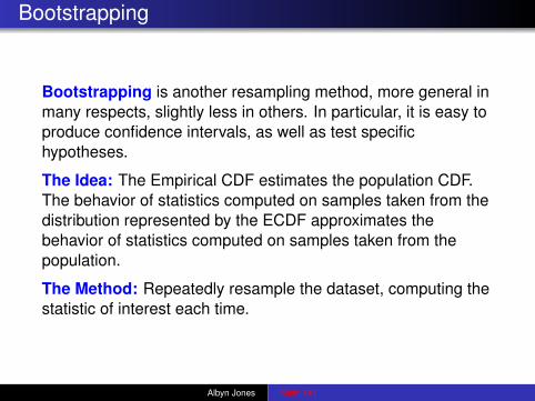
Bootstrapping is another resampling method, more general inmany respects, slightly less in others. In particular, it is easy toproduce confidence intervals, as well as test specifichypotheses.
The Idea: The Empirical CDF estimates the population CDF.The behavior of statistics computed on samples taken from thedistribution represented by the ECDF approximates thebehavior of statistics computed on samples taken from thepopulation.
The Method: Repeatedly resample the dataset, computing thestatistic of interest each time.
Albyn Jones Math 141
Example: Simple 95% CI for difference of means
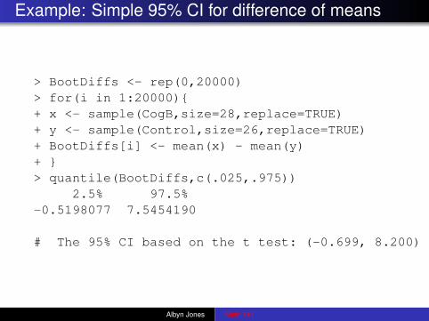
> BootDiffs <- rep(0,20000)> for(i in 1:20000){+ x <- sample(CogB,size=28,replace=TRUE)+ y <- sample(Control,size=26,replace=TRUE)+ BootDiffs[i] <- mean(x) - mean(y)+ }> quantile(BootDiffs,c(.025,.975))
2.5% 97.5%-0.5198077 7.5454190
# The 95% CI based on the t test: (-0.699, 8.200)
Albyn Jones Math 141
Another Bootstrap CI
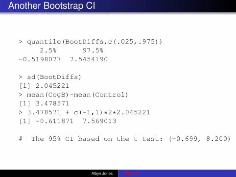
> quantile(BootDiffs,c(.025,.975))2.5% 97.5%
-0.5198077 7.5454190
> sd(BootDiffs)[1] 2.045221> mean(CogB)-mean(Control)[1] 3.478571> 3.478571 + c(-1,1)*2*2.045221[1] -0.611871 7.569013
# The 95% CI based on the t test: (-0.699, 8.200)
Albyn Jones Math 141
Bootstrapping Paired Samples
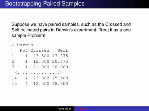
Suppose we have paired samples, such as the Crossed andSelf polinated pairs in Darwin’s experiment: Treat it as a onesample Problem!
> DarwinPot Crossed Self
1 1 23.500 17.3752 1 12.000 20.3753 1 21.000 20.000<................>
14 4 23.000 15.50015 4 12.000 18.000
Albyn Jones Math 141
Example: Darwin’s Data
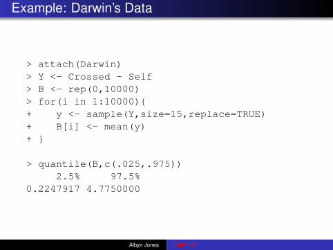
> attach(Darwin)> Y <- Crossed - Self> B <- rep(0,10000)> for(i in 1:10000){+ y <- sample(Y,size=15,replace=TRUE)+ B[i] <- mean(y)+ }
> quantile(B,c(.025,.975))2.5% 97.5%
0.2247917 4.7750000
Albyn Jones Math 141
Compare to the T-test
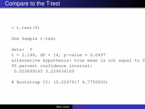
> t.test(Y)
One Sample t-test
data: Yt = 2.148, df = 14, p-value = 0.0497alternative hypothesis: true mean is not equal to 095 percent confidence interval:0.003899165 5.229434169
# Bootstrap CI: (0.2247917 4.7750000)
Albyn Jones Math 141
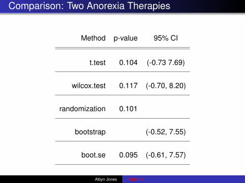
Comparison: Two Anorexia Therapies
Method p-value 95% CI
t.test 0.104 (-0.73 7.69)
wilcox.test 0.117 (-0.70, 8.20)
randomization 0.101
bootstrap (-0.52, 7.55)
boot.se 0.095 (-0.61, 7.57)
Albyn Jones Math 141
The R boot package
There is an R library with more sophisticated bootstrappingfunctions: package boot:
install.packages("boot")library(boot)?boot
Albyn Jones Math 141
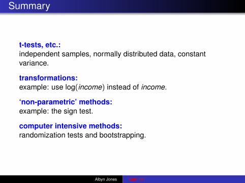
Summary
t-tests, etc.:independent samples, normally distributed data, constantvariance.
transformations:example: use log(income) instead of income.
‘non-parametric’ methods:example: the sign test.
computer intensive methods:randomization tests and bootstrapping.
Albyn Jones Math 141