Pushing back the boundaries: new techniques for assessing ... · Pushing back the boundaries: new...

Pushing back the boundaries:new techniques forassessing the impactof burglary schemes

Home Office Online Report 24/03

Kate BowersShane JohnsonAlex Hirschfield

The views expressed in this report are those of the authors, not necessarily those of the Home Office (nor do theyreflect Government policy).

The Research, Development and Statistics Directorate

RDS is part of the Home Office. The Home Office's purpose is to build a safe, just and tolerantsociety in which the rights and responsibilities of individuals, families and communities areproperly balanced and the protection and security of the public are maintained.

RDS also part of National Statistics (NS). One of the aims of NS is to inform Parliament andthe citizen about the state of the nation and provide a window on the work and performanceof government, allowing the impact of government policies and actions to be assessed.

Therefore -

Research Development and Statistics Directorate exists to improve policy making, decisiontaking and practice in support of the Home Office purpose and aims, to provide the publicand Parliament with information necessary for informed debate and to publish informationfor future use.

First published 2003Application for reproduction should be made to Communication Development Unit, Room201, Home Office, 50 Queen Anne’s Gate, London SW1H 9AT.© Crown copyright 2003 ISBN 1 84082 838 2

Foreword

Reducing Burglary Initiative EvaluationThe Reducing Burglary Initiative

In 1998 the Home Office announced the Crime Reduction Programme. The programme wasintended to develop and implement an integrated approach to reducing crime and makingcommunities safer. The Reducing Burglary Initiative (RBI), launched in 1999, was one of thefirst parts of this programme to commence.

The aims of the RBI are to:

l reduce burglary nationally by targeting areas with the worst domestic burglary problems;

● evaluate the cost effectiveness of the different approaches and; ● find out what works best where.

Two hundred and forty seven burglary reduction projects have been funded, covering over2.1million households that suffered around 110,000 burglaries a year. Three distractionburglary projects have also been funded.

The EvaluationThree consortia of universities have intensively evaluated the first round of 63 RBI projects.A further five projects from subsequent rounds of the RBI (rounds two and three) are alsobeing evaluated.

This report is part of a series of studies examining burglary reduction practice beingpublished during 2003. Also to be published are a summary and full report on the overallimpact and cost-effectiveness of Round 1 of the RBI. Other themes to be covered in thisseries are:

● the delivery of burglary reduction projects;● police detection strategies;● publicity and awareness of burglary reduction schemes; and ● the use of alley-gates as a means to reduce burglary.

i

Published reportsEarly lessons from the RBI have already been published in the following reports, which areavailable from www.homeoffice.gov.uk/rds/pubsintro1.html

Tilley N, Pease K, Hough M and Brown R (1999) ‘Burglary Prevention: Early Lessons fromthe Crime Reduction Programme’ Crime Reduction Research Series Paper 1, London: HomeOffice

Curtin L, Tilley N, Owen M and Pease K (2001) ‘ Developing Crime Reduction Plans: SomeExamples from the Reducing Burglary Initiative’ Crime Reduction Research Series Paper 7,London: Home Office

Hedderman C and Williams C (2001) ‘ Making Partnership Work: Emerging Findings fromthe Reducing Burglary Initiative’ Briefing Note 1/01, London: Home Office

Johnson S and Loxley C (2001) ‘ Installing Alley-gates: Practical Lessons from BurglaryPrevention Projects’ Briefing Note 2/01, London: Home Office

ii

iii

Acknowledgements

The authors would like to thank Merseyside Police and members of the Safer MerseysidePartnership for supplying information that was essential to the research described in thisreport. Our thanks also go to Jacque Mallender, Andy Richman and Peter Jordan at MHAConsultants for their helpful comments on earlier drafts of this paper. The authors would liketo thank the other members of the Northern Consortium, who were involved with theReducing Burglary Initiative (RBI) evaluation, and in particular Chris Young, for hisassistance with data processing.

The authors

Kate Bowers and Shane Johnson are Research Fellows at the Environmental CriminologyResearch Unit (ECRU) at the Department of Civic Design, University of Liverpool. Their mainrole in the evaluation has been in the creation and application of quantitative methods tomeasure changes in patterns of victimisation, some of which are described here. AlexHirschfield is a Reader in Planning, also based at ECRU in the University of Liverpool. He isthe Principal co-ordinator of the Northern Consortium, formed to undertake the evaluation of21 burglary reduction schemes in the north of England.

The Home Office, RDS Crime and Policy Group would like to thank Trevor Bennett, Professorof Criminology at the University of Glamorgan, and Ross Homel, Professor of Criminology &Criminal Justice at Griffith University, Queensland, who acted as independent assessors forthis report.

iv

Contents

PageForeword i

Acknowledgements ii

List of tables v

List of figures v

Main findings vii

Executive summary ix

1. Introduction 1Liverpool case study 2Contextual information 5

2. Changes in the burglary rate 9Statistical significance testing 10Targeted versus non-targeted areas of SDP 12

3. Repeat victimisation 15Methodology 15Levels of repeat victimisation in the SDP and BCU 15

4. Displacement 17Geographical displacement 17Crime switch displacement 19Target switch 27

5. Effectiveness of interventions 29Measuring the effects of a single intervention 29Measuring the effects of multiple interventions 32

6. The influence of other initiatives 35

7. Concluding remarks 37

Appendix 1 43Appendix 2 45

References 47

List of tables

1.1 Socio-demographic profile of the scheme and comparison areas 7

5.1. Domestic burglaries and repeats in target hardened properties before and after SDP became active 30

5.2. Revised table examining burglaries that happened after inception date in relation to their individual target hardening date 31

5.3. Outcomes for target hardening scheme 325.4. Outcomes for different types of treatment 34

List of figures

1.1 Liverpool Strategic Development Project Area 32.1 Burglary rates before and after the SDP began 102.2. Changes in the burglary rate for police beats 122.3 Quarterly crime rates in targeted and non-targeted areas 133.1. Proportion of burglaries that were incidents of

repeat victimisation 164.1 Weighted displacement quotients for the five buffer rings 194.2 Theft of car rates before and after the SDP began 204.3 Theft from car rates before and after the SDP began 214.4. Changes in the distribution of burglary before and

after scheme inception 254.5 Changes in the distribution of theft from vehicle

before and after scheme inception 264.6 Reduction in burglary rates for different groups of property 27

v

Main findings

This report describes the main findings of a detailed evaluation of a burglary reductionproject located in Liverpool in the North of England. The scheme consisted of fourinterventions: alley-gating, target hardening of property, property marking and an offenderrehabilitation intervention. New analytical techniques, discussed in detail in this report,were developed in order to answer the key evaluation questions. The results may besummarised as follows:

● Identifying the precise geographical areas in which crime preventioninterventions are implemented is important in assessing the effectiveness ofschemes. For the Liverpool scheme, the official boundary of the target areawas defined as two complete police beats, although the interventions werefocused almost exclusively within three sub-areas. Analyses revealed thatburglary reduction was dramatic in the sub-areas of intense implementationwithin the official boundary of the scheme.

● Statistical analysis, comparing the police beats that made up the scheme areato other police beats in Merseyside, showed that the reduction in burglary wasstatistically significant.

● Repeat burglary, as well as single incidents of burglary, significantly reducedin the scheme area.

● Analyses of crime rates in the areas that surrounded the scheme suggested thatthere was some evidence of geographical displacement. However, in a bufferzone that was within very close vicinity of the scheme, a diffusion of benefit(i.e. a reduction in burglary) was also evident.

● There was some evidence that following the implementation of the scheme offenders mayhave switched to committing other types of crime within the scheme area. In particular,theft from car significantly increased in the area. There was no significant switch to theftfrom a person, taking a vehicle without thse owners consent or theft of car.

vii

viiiviii

● In the sub-areas where crime prevention activity was concentrated, there wasevidence of a diffusion of benefit to untreated households. In other words,burglary reduced in both those properties that had been treated and those thathad not.

● In order to get the most accurate assessment of the effectiveness of crimeprevention strategies aimed at individual properties, it is necessary to examinethe pattern of victimisation of these properties over time. Doing this for theLiverpool scheme revealed that 13 burglaries were prevented in a one-yearperiod across 363 properties that had been target hardened. Moreover, therisk to these properties was almost halved following target-hardening. Thisexercise was done for each intervention type.

● Assessment should be made of the degree to which other initiatives in ascheme area are likely to cause burglary reduction. In the Liverpool scheme, itwas concluded that such initiatives were unlikely to have contributed to thereduction found.

The implications of these results for crime prevention are discussed in the report.

ixix

Executive summary

This report is a result of evaluation research undertaken in the north of England, thatwas commissioned by the Home Office to assess the impact of burglary projects fundedunder the first round of the Reducing Burglary Initiative (RBI). This paper, which focuseson one burglary scheme undertaken in Liverpool, demonstrates the power of usingdisaggregate, or individual level, burglary data in assessing the impacts and outcomesof such schemes, and illustrates that very different conclusions may be drawn when suchanalyses are not conducted.

The first three procedures described examine methods of measuring the impact of crimereduction schemes on levels of burglary (and other crimes) within the operationalboundaries of the initiative. These concern:

Measuring changes in the burglary rate

This compares changes in the burglary rate within the boundary of the scheme with a seriesof comparison areas. The comparison areas included one police beat, matched on socialand economic characteristics with the scheme’s operational area, the wider police BasicCommand Unit (BCU) and the wider Police Force Area (PFA). Importantly, changes in theburglary rate for the entire scheme area (which is the only analysis possible with aggregatelevel data) are compared with changes in smaller sub-areas of the scheme into whichtreatment was concentrated. The analysis revealed that the scheme had a substantial impacton the burglary rate for the sub-areas in which crime reduction activity was almostexclusively concentrated, but that the change in the burglary rate was relatively modest forthe entire scheme area. This finding demonstrates that sub-scheme analysis is essential inmeasuring the real impact of measures taken, particularly when initiatives aregeographically concentrated.

Statistical procedures for assessing impact

In order to assign statistical significance to changes in the burglary rate in the scheme area,a method was developed that compared these changes with those experienced in otherpolice beats throughout the county of Merseyside. Specifically, z-tests were undertaken to

see whether the reduction in burglary in the scheme area was significantly different fromthat seen in police beats in general. Results demonstrated that changes in the burglary ratefor the scheme area, and in particular for the sub-areas, were statistically significant.

Examining the distribution of repeat victimisation

This section highlights the importance of examining the concentration as well as theincidence and/or prevalence of burglary. There was evidence that levels of repeat burglary,as well as burglary per se, had decreased disproportionately in the scheme area whencompared with the comparison areas. Interestingly, decreases in the repeat rate weredetected in areas that had not experienced a decrease in burglary per se. This illustratesthat to fully understand the impact of crime reduction activity, it is necessary to considerrepeat victimisation in addition to simple burglary rates.

The paper proceeds to consider the possibility of crime displacement; that is, whether themeasures taken as part of the burglary reduction scheme caused local burglary offenders tochange their offending behaviour by targeting other properties, other areas or other types ofcrime. Therefore, three different types of displacement are considered here:

Geographical displacement

This describes a method for assessing the extent to which offenders move to other areas tocommit burglary as a result of the action being taken. Pre and post-intervention burglaryrates were examined in the target area, a buffer zone that surrounded the scheme, and thewider police force area. The theoretical rationale for the analysis was three-fold:

1. For displacement to occur there should be a reduction in the burglary rate for thetarget area indicating that offenders were avoiding this area (to some extent),thereby increasing the possibility that they would target alternative areas.

2. That coincident with this change the crime rate in the buffer zone should increase.

3. Finally, that the changes observed in both the target and buffer zone areas shouldexceed those observed in the wider police force area, thereby demonstrating thatthey did not simply reflect a more general trend.

xx

Detailed analysis considered change in the crime rates for a series of five smallerdisplacement buffer zones contained within the general buffer area. The method ofcalculation (which calculates a ‘weighted displacement quotient’ WDQ) therefore compareschanges in the burglary rates for these five different (but nested) areas over time. Briefly, asingle statistic is produced which describes the extent to which displacement (or, of course,diffusion of benefit) is likely to have occurred. Positive WDQ values indicate diffusion ofbenefit to the buffer zone and negative WDQ values indicate geographical displacement ofcrime. Considering the WDQ values, a figure of +1 indicates a diffusion of benefit wherethe burglary reduction in the buffer zone is equal to that in the project area. A figure of –1indicates a displacement where the burglary reduction is entirely offset by increases in thebuffer zone. A WDQ of zero represents a scenario where there was apparently no changein the buffer zone, or where this change could not be attributed to changes in the SDP.

Results of the analysis showed some evidence of geographical displacement as a result ofthe Liverpool scheme. Interestingly, there was evidence of a diffusion of benefit in theimmediate vicinity of the scheme. In contrast, there was substantial evidence ofdisplacement at a distance of approximately 400 metres or more from the operationalboundary of the scheme. In addition, the pattern of results suggested that there wasevidence of a distance-decay effect, with the extent of geographic displacement dissipatingacross greater distances.

Crime type switch

This assesses the extent to which the action taken causes offenders operating within thescheme area to switch to perpetrating offences of other types of crime. The analysis waslimited to other types of property crime, namely theft from a person, taking of a vehiclewithout the owner's consent, theft of car and theft from car. It was found that very differenttrends were observed in these crime types. Crucially, although theft of car did not appear tobe affected in the area, theft from car increased very significantly when compared withchanges observed in the comparison areas. Further analysis revealed that this pattern ofresults was statistically significant. It is hypothesised that the reason for this switch is that theskills required for committing theft from car and burglary are very similar and they are bothlikely to yield goods that can be sold on for financial gain.

xixi

Target switch

A third type of displacement that may result from crime reduction activity is that of targetswitch. It is possible that where certain houses have been treated on a street (e.g. by targethardening measures), offenders will simply target other properties that have not receivedtreatment. This issue was investigated by identifying all treated and untreated properties inthe sub-areas of the scheme in which crime reduction activity was concentrated. Changes inburglary rates were calculated for both groups of properties. Interestingly, relative to thedrop in burglary in the treated properties, burglary rates in the non-treated properties fellalmost as much. This effect was not observed in any of the comparison areas, nor, indeed,for the rest of the scheme areas (those outside the three sub-areas). This shows a very localdiffusion of benefit effect, whereby houses situated near to treated properties also appear tohave been avoided by offenders after the measures were installed.

The procedures discussed above outline methods of assessing impacts of burglary schemesas a whole. However, it is important to remember that it is very unusual for schemes toconcentrate solely on one intervention. Far more commonly, schemes involve undertaking anumber of different interventions to combat a burglary problem. In the case of Liverpool, forexample, four different interventions were involved: target-hardening, property marking(Smartwater), alley-gating and an offender behaviour scheme. In order to start to understandwhat it is that makes a scheme successful, it is important to try to isolate the impact of theindividual interventions undertaken. Therefore methods were developed which:

● Can be used to assess the impact of individual interventions

This technique uses information on the actual individual properties that weretreated as part of an intervention. For illustrative purposes, this section focuseson target-hardening. It was found that by examining levels of burglary in theseproperties by simply taking the overall start date of the scheme to define beforeand after periods, the target hardening intervention appeared to be veryineffective. However, further analyses that used information concerned with theactual date of target hardening for each property revealed a very differentpicture. The method described also corrects for differences in opportunity dueto the fact that the before and after target-hardening periods examined willvary depending on the exact date of target hardening. These ‘opportunity-dependent rates’ are then used to calculate an outcome in terms of the numberof burglaries prevented by the intervention, by comparing the after targethardening rate to an expected rate produced using the before period. The

xiixii

method also takes into account general changes in the burglary rate at thecounty level over time. Results indicated that the target hardening intervention,which involved 363 properties, prevented 13 burglaries in a one-year period.

● Apply this method to each intervention type

This opportunity-dependent rate method was used to calculate outcomes foreach of the three geographically targeted interventions in the Liverpool schemearea (that is, target hardening, alleygating and property marking). Onecomplication is that individual properties could receive up to three of thesetreatments. In other words, whilst some properties only received targethardening, others could have received target hardening and property marking,target hardening and alleygating, or, indeed, all three measures. Outcomeswere therefore calculated for each of the possible combinations ofinterventions. Results indicated that target hardening, either on its own or incombination with other interventions, appeared to be particularly effective.

A final section addresses the issue of other crime reduction efforts, which could potentiallyhave a confounding effect on the outcome analysis described in the report. Other crimereduction and regeneration activities were operating in the area within the timescale of theLiverpool SDP. However, these other schemes were implemented across wide areas of thecity of Liverpool. For this reason, it can be assumed that the BCU, the comparison area andthe buffer zone of the SDP would all have been affected by these other initiatives. Thismeans that to a certain degree the influence of other initiatives was controlled for. The reportconcludes that ‘other interventions’ were unlikely to have contributed to the changeobserved in the scheme area.

xiiixiii

1. Introduction

As far as we are aware, the majority of published crime reduction evaluations have, in thepast, utilised recorded crime (and other) data that is aggregated to particular geographicalarea units such as police beats or local authority wards. Whilst the use of such data enablesevaluators to determine the effects of a particular scheme at the general area level, it clearlyprecludes the computation of more sophisticated analyses. Such analyses should, critically,allow specific a priori (and, of course, post hoc) hypotheses to be tested that may potentiallyexplain why a particular scheme was or was not successful, or whether it was successful insome respects but not others. For instance, for a target-hardening scheme, whilst the crimerate for the general area in which the scheme operates may be unaffected, target-hardenedhouseholds may experience significantly lower levels of victimisation than would have beenexpected had the scheme not existed. Alternatively, although the burglary crime rate mayremain unchanged, levels of repeat victimisation may be dramatically reduced. In addition,and importantly, the use of aggregate level data also limits the investigation of whether therewere any unexpected side effects, or spin-offs of the scheme, such as the geographicaldisplacement of crime. To do this type of analysis, one would require disaggregate leveldata, which provides data concerning individual incidents of crime and includes informationon the address, geographical location (e.g. an easting and northing grid reference) anddate of the offence (for a further discussion of this issue, see Johnson et al, 2001). Studiesthat have used disaggregate level crime data (e.g. Anderson et al, 1995; Bennett andDurie, 1999), whilst being insightful have been limited to analyses of rates of victimisationand repeat victimisation at the area level only.

In 1999 the Home Office launched the RBI, a multi million pound initiative aimedspecifically at reducing domestic burglary. A total of 63 projects were commissioned in thefirst round which varied considerably in terms of the interventions they employed, althoughmost had a strong situational crime reduction focus. Of these, 21 were commissioned in thenorth, Midlands and south of England respectively (for more details, see Tilley et al, 1999).In addition to funding the projects themselves, the Home Office commissioned threeevaluation consortia to evaluate the schemes operating in the different regions. Theconsortium commissioned to evaluate the schemes operating in the North of Englandcomprises research groups based at three different universities, these being theEnvironmental Criminology Research Unit (ECRU) at the University of Liverpool, the AppliedCriminology Group (ACG) at the University of Huddersfield, and the Centre of Criminologyand Criminal Justice at the University of Hull.

1

Part of the evaluation design adopted by the Northern consortium was to conduct in-depthcase studies for each of the schemes using disaggregate level data. However, for numerousreasons, one of the most influential being police data protection procedures, the Northernconsortium was unable to obtain such data for three of the five police force areas that coverthe northern region. In addition, data for one of the police forces was obtained at a verylate stage in the evaluation. Taken together, these problems limited the number of casestudies that could be conducted. However, links between the evaluators and the MerseysidePolice Force led to the consortium having access to this information for Merseyside from thebeginning of the evaluation. Therefore, the Liverpool Strategic Development Project (SDP)has been selected as a case study to demonstrate the sophistication of the analysis that ispossible where good information is available and to illustrate some of the new techniquesdeveloped for the evaluation.

The current report will first discuss the Liverpool scheme and the interventions employed, andthen present analyses concerned with the outcome of the scheme. Particular emphasis willbe placed upon the new techniques developed to measure the statistical significance of anychanges in the crime rate for the target area, the effectiveness of target-hardening and theextent to which geographical, crime-type and target-switch displacement were evident.Other sections will consider changes in the rate of repeat victimisation, and a novelapproach to mapping the change in crime rates.

The Liverpool case study

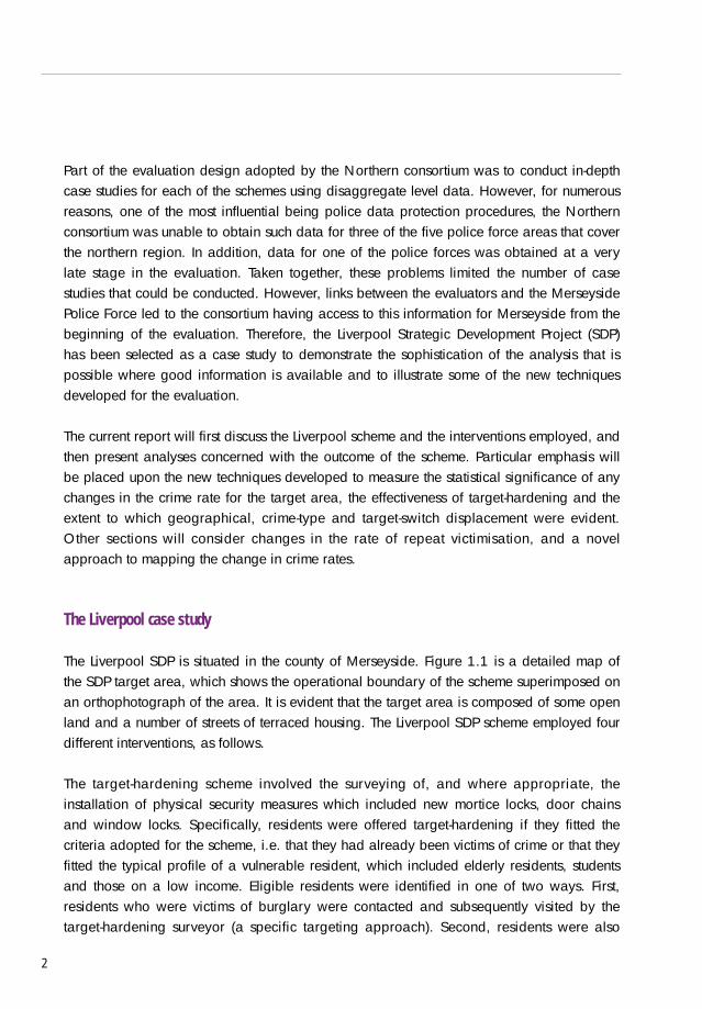
The Liverpool SDP is situated in the county of Merseyside. Figure 1.1 is a detailed map ofthe SDP target area, which shows the operational boundary of the scheme superimposed onan orthophotograph of the area. It is evident that the target area is composed of some openland and a number of streets of terraced housing. The Liverpool SDP scheme employed fourdifferent interventions, as follows.

The target-hardening scheme involved the surveying of, and where appropriate, theinstallation of physical security measures which included new mortice locks, door chainsand window locks. Specifically, residents were offered target-hardening if they fitted thecriteria adopted for the scheme, i.e. that they had already been victims of crime or that theyfitted the typical profile of a vulnerable resident, which included elderly residents, studentsand those on a low income. Eligible residents were identified in one of two ways. First,residents who were victims of burglary were contacted and subsequently visited by thetarget-hardening surveyor (a specific targeting approach). Second, residents were also

2

visited as part of a more general strategy, whereby the surveyor visited all householdscontained within the target area. This two-level approach ensured that burglary victims wereassisted as close to the incidents’ occurrence as possible.

Figure 1.1: Liverpool Strategic Development Project Area (sub-areas shaded in white)

The Smartwater intervention involved the marking of residents’ personal property to increasethe likelihood of stolen property being recovered, and to discourage offenders from burglingprotected properties. Smartwater is essentially a chemical solution, undetectable to thehuman eye unless examined under ultra-violet light, that is applied to items of personalproperty. The solution itself represents a chemical marker, for which the chemical sequencehas an almost limitless number of combinations. With the right equipment it is possible toidentify a particular Smartwater code or sequence. The approach adopted by the Liverpoolteam was to property mark personal property for households located on different streetsusing different versions of the solution, meaning that any recovered property could beidentified as belonging to an individual living on a specific street. Additional informationincluding a description of each item of property was recorded on a computer database,meaning that for any item of recovered (marked) property the actual owner should beidentifiable. To ensure that any recovered items of personal property could be identified,

3

ultra-violet lights were installed in the police stations that service the target area and policeofficers received training regarding the intervention. For each household, residents had upto ten items of personal property marked using smartwater. In addition, as a deterrent tooffenders, all households that had been property marked in this way were given a sticker toput in their window, to indicate that they were part of the scheme. All residents who lived inthe specific target area were offered this intervention.

The third intervention was an alley-gating scheme that involved the installation of lockablehard-wearing gates to both ends of the alleyways at the rear of the properties, with the aimof restricting access to potential offenders. Due to legal requirements, prior to the installationof the gates it was necessary to obtain approval from the residents affected by the scheme.1

Thus, teams of surveyors, funded through levered-in resources, visited properties to seekresidents approval and to explain the scheme to them. As experienced by other schemes(see Johnson and Loxley, 2001), the legal process of applying for closure orders for each ofthe alleyways impeded the progress of this scheme. Thus, although all of the surveys werecompleted by May 2000, only ten of the 69 gates were installed before 1 April 2001.Thus, only these ten gates will be considered in the research described below.

The final scheme was an offender-based scheme named the ‘Wavertree Dordrecht project’.This involved the intensive supervision of offenders with the aim of changing their attitudestowards offending and their offending behaviour. This scheme, which is still ongoing, issupported both by Merseyside police and the probation service, who each provided onemember of staff to work on the project on a day to day basis. Home Office funding wasused to match fund (50 per cent) the salary for the probation officer for a period of oneyear. The scheme is aimed at offenders either on licence, or at the pre-trial stage ofsentencing who had committed burglaries within the target area. Offenders who met the

4

1 Where a back alley provides no right of way to any person other than the immediate residents - i.e. a privateright of way, many local authorities run alley-gating schemes which allow such alleys to be closed off with theconsent of all the residents. The Guidance for those involved in alley-gating is on the Home Office crimereduction website at www.crimereduction.gov.uk/gating.htm. Further guidance can be found in the Home officeBriefing Note 2/01 "Installing Alley-gates: Practical Lessons from Burglary Prevention Projects" which may beviewed on the Home Office website at www.homeoffice.gov.uk/rds/prgbriefpubs1.html

Where a back alley carries a public right of passage, a legal closure/diversion is necessary. The new provisionsin Sections 118B and 119B Highways Act 1980 allow an authority to apply to have an area that is a crime 'hotspot' designated, allowing rights of way within that area to be closed or diverted for crime reduction purposes.Local highway authorities will usually take the lead, working with crime and disorder reduction partnerships,police authorities, local residents and user groups to formulate a submission to the Secretary of State seeking theinclusion of an area, or areas, in a designation order. In county areas, the district authority or the local crimeand disorder reduction partnership may be able to make a submission if the county council is unwilling to do so.The authority will need to show (a) that the area has a right of way that can be shown to facilitate high levels ofpersistent crime and (b) that previous attempts to reduce crime in the area have been tried and found to beineffective Guidance is available online at: www.defra.gov.uk/wildlife-countryside/cl/publicrow.htm

criteria for the scheme were largely identified by colleagues in the probation service whohad been informed of the scheme. Once identified, offenders were approached by the staffand invited to participate. During the period 1 January 2000–31 March 2001 a total of sixoffenders had been recruited and had participated in the scheme.

These interventions do not all operate in the entire target area, and, in particular, the target-hardening, property marking and alley-gating initiatives were almost exclusivelyconcentrated within the three sub-areas shaded white in Figure 1.1. Since sub-areas wereused for three of the four interventions there is the possibility that the initiatives could havecaused some displacement of burglary within the target area. Moreover, it is also possiblethat any reductions in burglary rates would only have been observed in these areas.

The offender scheme is distinct from the other three interventions since it is notgeographically targeted in sub-areas of the target area. Furthermore, its approach toburglary reduction is rather more long-term, as it takes an offender –based, rather than asituational prevention-based, perspective. For these reasons, although the offenderintervention is accounted for in analyses that consider the overall effect of the scheme, itsindividual impact on burglary in the scheme area is not assessed in the analysis that follows.

Contextual information

More specific contextual data for the SDP area is available from the 1991 PopulationCensus, and the left hand column of Table 1.1 summaries some of the socio-demographiccharacteristics of the SDP. The Table shows that the area is made up of 3317 households, ofwhich the majority of houses are terraced properties, making up 79.4 per cent of the totalhouseholds in the area. There is also a substantial percentage of flats and bedsits in thearea (14.5 per cent). Interestingly, the SDP area is not as deprived as some of the otherSDPs in the Northern Consortium area; there is a high percentage of households that areowner occupied (70.4 per cent) and a lower than average number of households without acar (44.9 per cent compared to a consortium average of 55 per cent).2

Part of the evaluation methodology adopted involves defining and studying crime trends in aseries of comparison areas for each of the 21 projects. These areas include the remainder ofthe police force area (PFA–SDP), the remainder of the police basic command unit (BCU–SDP)in which the SDP is located and a further area with a socio-demographic profile as similar to

5

2 It should be noted that because all these figures are taken from the 1991 census, it is likely that some of thisinformation is out-of-date. However, since the SDP area is mainly composed of well-established older housing,the housing stock of the area is unlikely to have changed dramatically over the last ten years. Although the SDParea did not conform to census geography, a procedure that makes a correction for this boundary problem wasused that has been described in full elsewhere (Hirschfield and Bowers, 1997).

the SDP as possible. This last area, which will subsequently be referred to as the ‘comparisonarea’, was selected through an iterative search process using a geographical informationsystem (GIS). The criteria for selecting the comparison area were as follows:

● that the area conformed to police beat geography;

● that it was in the same local authority district as the target area;

● that it was as similar as possible to the target area in terms of its socio-economic makeup;

● that it was not contiguous with the SDP (to ensure that changes in this areacould not simply be attributed to geographical displacement from the SDP).

The right hand column of Table 1.1 shows that the SDP and the comparison area are similar interms of census variables. As is the case with the SDP area itself, the comparison area is primarilycomposed of terraced houses and has a high percentage of households that are owner-occupied.In addition, it has very similar levels of households without a car to the target area.

This section has provided contextual information on the SDP and comparison areas. The rest ofthis paper will examine changes in the burglary rate and distribution of crime since the SDP hasbeen operational. The first section looks at these changes and at the issue of repeat victimisation,whilst sections 2 to 4 consider three different types of displacement. These are geographicdisplacement, which is said to have occurred when offenders commit crimes that they would havecommitted in the target area in a buffer zone that surrounds the target area; crime-switch,whereby offenders commit other types of (replacement) crime(s) instead of burglary; and target-switch, where offenders still commit crimes within the target area(s) but select individual propertiesthat have not been subject to the crime reduction strategy. Section 5 focuses on the individualtarget hardening of properties in the area and its effect on burglary rates. Section 6 expands onthis by assessing the impact of other interventions implemented by the scheme. Finally section 7considers the potential effect of other crime reduction initiatives in the SDP area on changes in thelevel of burglary within the scheme area.

6

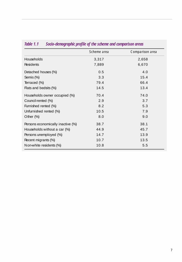
Table 1.1 Socio-demographic profile of the scheme and comparison areas

Scheme area Comparison area

Households 3,317 2,658Residents 7,889 6,670

Detached houses (%) 0.5 4.0Semis (%) 3.3 15.4Terraced (%) 79.4 66.4Flats and bedsits (%) 14.5 13.4

Households owner occupied (%) 70.4 74.0Council-rented (%) 2.9 3.7Furnished rented (%) 8.2 5.3Unfurnished rented (%) 10.5 7.9Other (%) 8.0 9.0

Persons economically inactive (%) 38.7 38.1Households without a car (%) 44.9 45.7Persons unemployed (%) 14.7 13.9Recent migrants (%) 10.7 13.5Non-white residents (%) 10.8 5.5

7

9

2. Changes in the burglary rate

Disaggregate level data concerned with burglary, covering the period 1 April 1997 to 31March 2001, was obtained for the county of Merseyside. This data, extracted fromMerseyside Police Force’s Integrated Criminal Justice System (ICJS) includes the followingfields of data: a unique crime reference number; crime code; the address where theburglary took place; an easting and northing grid reference accurate to within one-metre;and the date and time of the offence.

These data were used to provide historic data that covered the two-year period thatpreceded the start of the project (April 1999), and data that covered the two-year period 1April 1999 to 31 March 2001 during which the SDP was active. This data was thencleaned using software generated by the researchers (Johnson et al, 1997) which amongstother things, identifies and discards duplicate records, those without grid references, thosewithout dates, and those without sufficient information to uniquely identify the address of theoffence (e.g. 21 The Road – an address without indication of the area or postcode). Theclean data (the incident counts for which are shown in Appendix 2) was used to computeburglary rates for the SDP, the BCU, the Police Force Area (PFA) and other areas of interest.

A further issue that warrants discussion is the fact that whilst the target area is defined astwo police beats, as noted above three of the four interventions (target hardening,smartwater and alleygating) were almost exclusively confined to three sub-areas within theSDP. For this reason, maps of the three sub areas were obtained, and the boundaries weredigitised and imported into a GIS. This allowed us to calculate crime rates for the sub-areawithin the SDP where the three types of measure were concentrated and the remainder ofthe SDP that had received very little attention in terms of physical security upgrades. Figure2.1 shows the burglary rates for six different areas for the period before and after inceptionof the Liverpool SDP (that is 1 April 1997–31 March 1999 and 1 April 1999–31 March2001 respectively). These areas are the SDP as defined by its entire operational boundary,the sub-area of the SDP in which the situational crime reduction measures were focused, theremainder of the SDP (where there was little or no activity), the comparison area, the BCU inwhich the SDP was located, and the PFA.

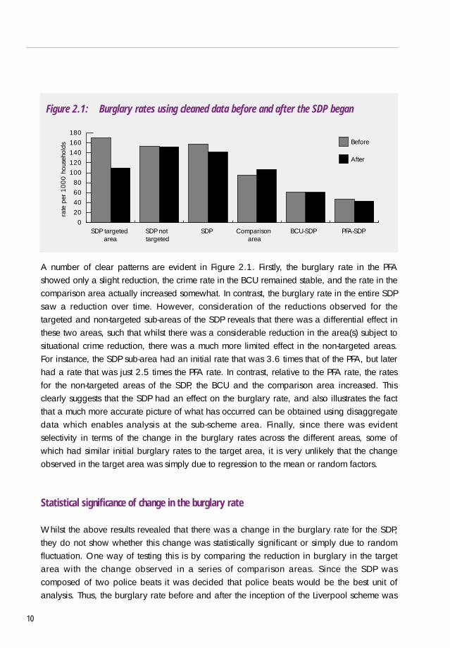
Figure 2.1: Burglary rates using cleaned data before and after the SDP began

A number of clear patterns are evident in Figure 2.1. Firstly, the burglary rate in the PFAshowed only a slight reduction, the crime rate in the BCU remained stable, and the rate in thecomparison area actually increased somewhat. In contrast, the burglary rate in the entire SDPsaw a reduction over time. However, consideration of the reductions observed for thetargeted and non-targeted sub-areas of the SDP reveals that there was a differential effect inthese two areas, such that whilst there was a considerable reduction in the area(s) subject tosituational crime reduction, there was a much more limited effect in the non-targeted areas.For instance, the SDP sub-area had an initial rate that was 3.6 times that of the PFA, but laterhad a rate that was just 2.5 times the PFA rate. In contrast, relative to the PFA rate, the ratesfor the non-targeted areas of the SDP, the BCU and the comparison area increased. Thisclearly suggests that the SDP had an effect on the burglary rate, and also illustrates the factthat a much more accurate picture of what has occurred can be obtained using disaggregatedata which enables analysis at the sub-scheme area. Finally, since there was evidentselectivity in terms of the change in the burglary rates across the different areas, some ofwhich had similar initial burglary rates to the target area, it is very unlikely that the changeobserved in the target area was simply due to regression to the mean or random factors.

Statistical significance of change in the burglary rate

Whilst the above results revealed that there was a change in the burglary rate for the SDP,they do not show whether this change was statistically significant or simply due to randomfluctuation. One way of testing this is by comparing the reduction in burglary in the targetarea with the change observed in a series of comparison areas. Since the SDP wascomposed of two police beats it was decided that police beats would be the best unit ofanalysis. Thus, the burglary rate before and after the inception of the Liverpool scheme was

10

020406080

100120140160180

SDP targeted area

SDP not targeted

SDP Comparison area

BCU-SDP PFA-SDP

rate

per

100

0 ho

useh

olds

Before

After

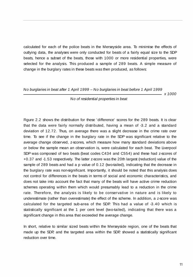
calculated for each of the police beats in the Merseyside area. To minimise the effects ofoutlying data, the analyses were only conducted for beats of a fairly equal size to the SDPbeats, hence a subset of the beats, those with 1000 or more residential properties, wereselected for the analysis. This produced a sample of 289 beats. A simple measure ofchange in the burglary rates in these beats was then produced, as follows:

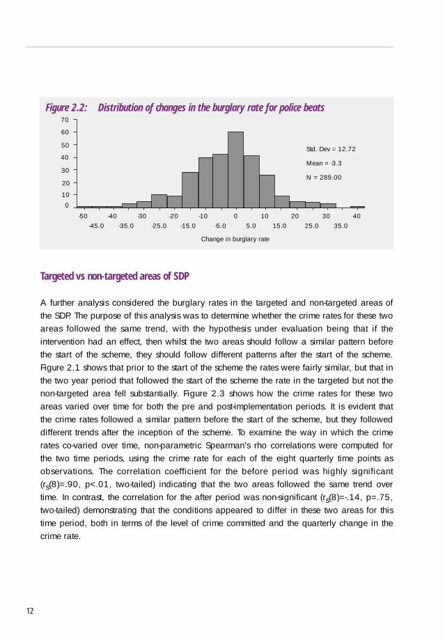
Figure 2.2 shows the distribution for these 'difference' scores for the 289 beats. It is clearthat the data were fairly normally distributed, having a mean of -3.2 and a standarddeviation of 12.72. Thus, on average there was a slight decrease in the crime rate overtime. To see if the change in the burglary rate in the SDP was significant relative to theaverage change observed, z-scores, which measure how many standard deviations aboveor below the sample mean an observation is, were calculated for each beat. The LiverpoolSDP was composed of two beats (beat codes C434 and C554) and these had z-scores of+0.37 and -1.53 respectively. The latter z-score was the 20th largest (reduction) value of thesample of 289 beats and had a p value of 0.12 (two-tailed), indicating that the decrease inthe burglary rate was non-significant. Importantly, it should be noted that this analysis doesnot control for differences in the beats in terms of social and economic characteristics, anddoes not take into account the fact that many of the beats will have active crime reductionschemes operating within them which would presumably lead to a reduction in the crimerate. Therefore, the analysis is likely to be conservative in nature and is likely tounderestimate (rather than overestimate) the effect of the scheme. In addition, a z-score wascalculated for the targeted sub-area of the SDP. This had a value of -3.40 which isstatistically significant at the 1 per cent level (two-tailed), indicating that there was asignificant change in this area that exceeded the average change.

In short, relative to similar sized beats within the Merseyside region, one of the beats thatmade up the SDP, and the targeted area within the SDP, showed a statistically significantreduction over time.

11

No burglaries in beat after 1 April 1999 – No burglaries in beat before 1 April 1999x 1000

No of residential properties in beat

70

60

50

40

30

20

10

-50 -40 -30 -20 -10-5.0 5.0

40302010

0

015.0 25.0 35.0-15.0-25.0-35.0-45.0

Std. Dev = 12.72

Mean = -3.3

N = 289.00

Change in burglary rate

Figure 2.2: Distribution of changes in the burglary rate for police beats

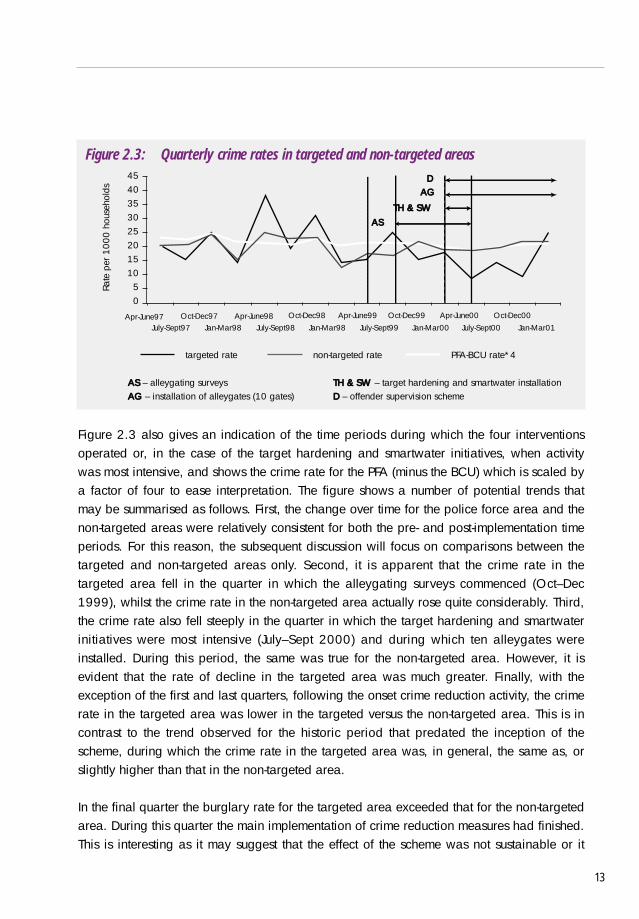
Targeted vs non-targeted areas of SDP

A further analysis considered the burglary rates in the targeted and non-targeted areas ofthe SDP. The purpose of this analysis was to determine whether the crime rates for these twoareas followed the same trend, with the hypothesis under evaluation being that if theintervention had an effect, then whilst the two areas should follow a similar pattern beforethe start of the scheme, they should follow different patterns after the start of the scheme.Figure 2.1 shows that prior to the start of the scheme the rates were fairly similar, but that inthe two year period that followed the start of the scheme the rate in the targeted but not thenon-targeted area fell substantially. Figure 2.3 shows how the crime rates for these twoareas varied over time for both the pre and post-implementation periods. It is evident thatthe crime rates followed a similar pattern before the start of the scheme, but they followeddifferent trends after the inception of the scheme. To examine the way in which the crimerates co-varied over time, non-parametric Spearman’s rho correlations were computed forthe two time periods, using the crime rate for each of the eight quarterly time points asobservations. The correlation coefficient for the before period was highly significant(rs(8)=.90, p<.01, two-tailed) indicating that the two areas followed the same trend overtime. In contrast, the correlation for the after period was non-significant (rs(8)=-.14, p=.75,two-tailed) demonstrating that the conditions appeared to differ in these two areas for thistime period, both in terms of the level of crime committed and the quarterly change in thecrime rate.

12

Rate

per

100

0 ho

useh

olds

05

1015202530354045

targeted rate non-targeted rate PFA-BCU rate*4

DAG

TH & SWAS

D – offender supervision schemeAG – installation of alleygates (10 gates)TH & SW – target hardening and smartwater installationAS – alleygating surveys

Apr-June97July-Sept97

Oct-Dec97Jan-Mar98


Oct-Dec98Jan-Mar98


Oct-Dec99Jan-Mar00


Oct-Dec00Jan-Mar01

Figure 2.3: Quarterly crime rates in targeted and non-targeted areas

Figure 2.3 also gives an indication of the time periods during which the four interventionsoperated or, in the case of the target hardening and smartwater initiatives, when activitywas most intensive, and shows the crime rate for the PFA (minus the BCU) which is scaled bya factor of four to ease interpretation. The figure shows a number of potential trends thatmay be summarised as follows. First, the change over time for the police force area and thenon-targeted areas were relatively consistent for both the pre- and post-implementation timeperiods. For this reason, the subsequent discussion will focus on comparisons between thetargeted and non-targeted areas only. Second, it is apparent that the crime rate in thetargeted area fell in the quarter in which the alleygating surveys commenced (Oct–Dec1999), whilst the crime rate in the non-targeted area actually rose quite considerably. Third,the crime rate also fell steeply in the quarter in which the target hardening and smartwaterinitiatives were most intensive (July–Sept 2000) and during which ten alleygates wereinstalled. During this period, the same was true for the non-targeted area. However, it isevident that the rate of decline in the targeted area was much greater. Finally, with theexception of the first and last quarters, following the onset crime reduction activity, the crimerate in the targeted area was lower in the targeted versus the non-targeted area. This is incontrast to the trend observed for the historic period that predated the inception of thescheme, during which the crime rate in the targeted area was, in general, the same as, orslightly higher than that in the non-targeted area.

In the final quarter the burglary rate for the targeted area exceeded that for the non-targetedarea. During this quarter the main implementation of crime reduction measures had finished.This is interesting as it may suggest that the effect of the scheme was not sustainable or it

13

could be due to lack of evidence of further physical implementation in the area leading tooffenders feeling it was safe to offend in the area once more. However, further data wouldbe required to confirm this. Taken together, the results show that there was a reduction in theburglary rate following the start of the scheme and that the reduction observed for thetargeted sub-areas appeared to coincide with a crude indicator of the timing of crimereduction activity.

14

15

3. Repeat victimisation

Methodology

To examine repeat victimisation the burglary data discussed above, and a further 12 monthsof historic data that covered the period 1 April 1996–31 March 1997, was analysed usingsoftware developed by the researchers (Johnson et al, 1996). This software was written inFORTRAN and works in the following way. The program developed reads in all the recordsconcerned with domestic burglary from a recorded crime file. A dynamic array,3 in whicheach element pertains to a unique address, is updated as the records are read in. When anew record is read in, the array is searched to see if a crime has already occurred at thataddress within the previous 12 months. If it has then the corresponding record is updated toindicate that a repeat occurred.4 However, if this is the first incident at the address, asreflected by the absence of the address in the array, then the new record is simply added tothe array. Alternatively, if the address supplied has too few characters to identify a uniqueaddress, or there is no grid reference, or the record is identified as a duplicate record bythe program, the record is discarded. The resulting array includes the following information:the addresses of all households which have been burgled, the number of incidents that haveoccurred at each address, and the dates on which each incident occurred.

Levels of repeat victimisation

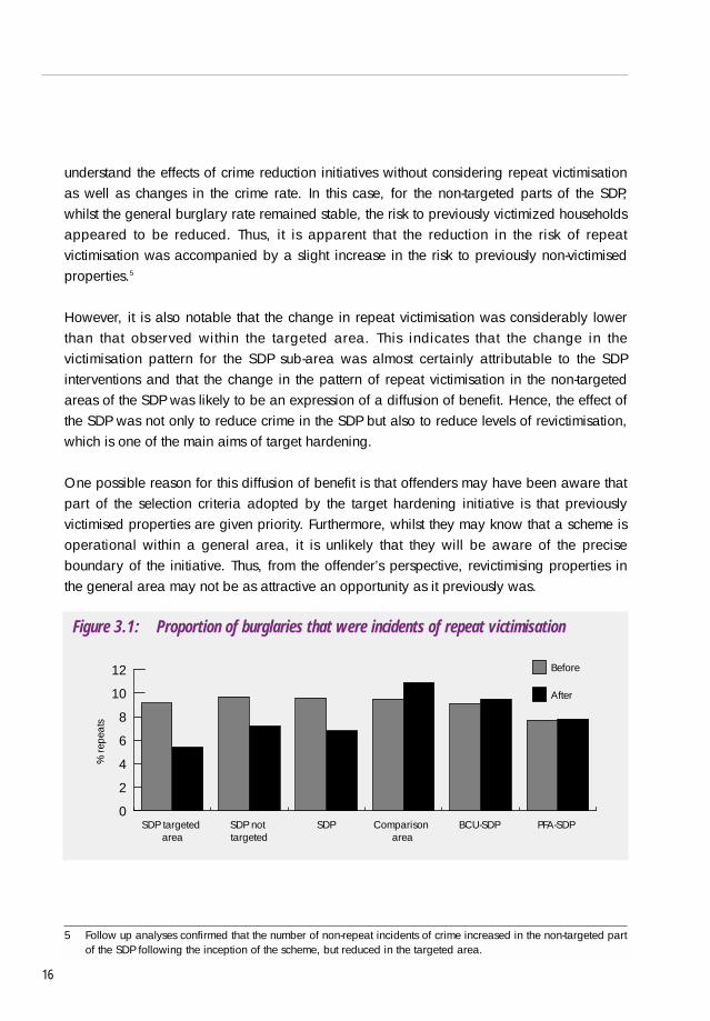
Figure 3.1 shows the levels of repeat burglary in each of the areas for the before and aftertime periods. It is apparent that, in general, levels of repeat victimisation actually increasedover time (1 per cent in the PFA and 4 per cent in the BCU). However, in the SDP, the levelof repeat victimisation actually fell by around 29 per cent. Moreover, for the SDP sub-areathe level fell by around 40 per cent, meaning that for this area the level of re-victimisationfell from a figure which was initially higher than that for the PFA, to a level that wasconsiderably lower than that for the PFA. Interestingly, whilst the crime rate did not showmuch of a reduction in the non-targeted areas of the SDP, the level of repeat victimisationdid (25 per cent reduction). This finding clearly illustrates that it is not possible to fully

3 An array is a form of data file that is stored in a computer’s memory, it is referred to here as a dynamic array toreflect the fact that the array increases in size as each new record is processed.

4 A complex address-matching algorithm was developed so that the program could determine whether twoaddresses were the same; this algorithm compensates, to some extent, for spelling mistakes and the inconsistencywith which addresses are stored on most police databases (For a discussion of the technique see Johnson et al.,1997; and for program code used, Johnson et al., 1996)

0

2

4

6

8

10

12 Before

After

SDP targeted area

SDP not targeted

SDP Comparison area

BCU-SDP PFA-SDP

% re

peat

s

understand the effects of crime reduction initiatives without considering repeat victimisationas well as changes in the crime rate. In this case, for the non-targeted parts of the SDP,whilst the general burglary rate remained stable, the risk to previously victimized householdsappeared to be reduced. Thus, it is apparent that the reduction in the risk of repeatvictimisation was accompanied by a slight increase in the risk to previously non-victimisedproperties.5

However, it is also notable that the change in repeat victimisation was considerably lowerthan that observed within the targeted area. This indicates that the change in thevictimisation pattern for the SDP sub-area was almost certainly attributable to the SDPinterventions and that the change in the pattern of repeat victimisation in the non-targetedareas of the SDP was likely to be an expression of a diffusion of benefit. Hence, the effect ofthe SDP was not only to reduce crime in the SDP but also to reduce levels of revictimisation,which is one of the main aims of target hardening.

One possible reason for this diffusion of benefit is that offenders may have been aware thatpart of the selection criteria adopted by the target hardening initiative is that previouslyvictimised properties are given priority. Furthermore, whilst they may know that a scheme isoperational within a general area, it is unlikely that they will be aware of the preciseboundary of the initiative. Thus, from the offender’s perspective, revictimising properties inthe general area may not be as attractive an opportunity as it previously was.

Figure 3.1: Proportion of burglaries that were incidents of repeat victimisation

16

5 Follow up analyses confirmed that the number of non-repeat incidents of crime increased in the non-targeted partof the SDP following the inception of the scheme, but reduced in the targeted area.

17

4. Displacement

The sections that follow will consider three different types of displacement in some detail. Toanticipate the findings, as with the results presented thus far, it will become apparent thatthe use of disaggregate data is essential for the analysis of crime displacement.


Geographical boundary dataThe actual SDP target area for the Liverpool scheme comprised two complete police beats (C434and C554). As shown in Figure 1.1, the boundary for the two beats was digitised and importedinto the GIS. Next, to examine geographical displacement, we defined a general buffer zonethat surrounded the SDP. To allow a more detailed analysis to be conducted, we defined five(rather than one) concentric buffer rings that had the same morphology as the boundary of thescheme area. The first buffer was produced so that it started at the SDP boundary and finished400 metres from the boundary at all points. This produces a band shape that mimics the SDPboundary all the way around. A further buffer was then created that began at the boundary ofthe first buffer and ended a further 400 metres from this boundary, so that the outside boundarywas 800 metres from the SDP boundary. Further buffers were created in the same way, until therewere five rings surrounding the SDP area. Using this system of concentric buffers, it was possibleto look at the change in the distribution of burglaries 0–400 ms, 400–800 ms……1600–2000ms away from the SDP area, to check for possible geographic displacement.

Calculating geographical displacement for each bufferTo measure the extent to which displacement or diffusion of benefit occurred, we used a newtechnique, the Weighted Displacement Quotient (WDQ: Bowers & Johnson, 2001), developedfor the evaluation. The WDQ technique is summarized in this section, and the equationpresented in Appendix 1. For an extended account along with a discussion of the researchliterature the interested reader is referred to Bowers and Johnson (in press). Essentially, theWDQ examines the change in the distribution of crime in the buffer zone(s) and compares thiswith the previous distribution of crime and with any changes in the PFA, and then relates thesepatterns to any changes observed in the target area. Critically, changes are measured relativeto the temporal distribution of crime in the PFA, and geographical displacement is onlyassumed to have occurred if a reduction occurs in the target area whilst there is an increase inthe buffer zone. In contrast, diffusion of benefit is presumed to have resulted if there is adecrease in both the target area and the buffer zone(s).

Positive WDQ values indicate diffusion of benefit to the buffer zone and negative WDQvalues indicate geographical displacement of crime. Considering the WDQ values, a figureof +1 indicates a diffusion of benefit where the burglary reduction in the buffer zone isequal to that in the project area. A figure of –1 indicates a displacement where the burglaryreduction is entirely offset by increases in the buffer zone. A WDQ of zero represents ascenario where there was apparently no change in the buffer zone, or where this changecould not be attributed to changes in the SDP.

It is important to note that should displacement occur, there is not necessarily a one-to-onerelationship between the number of burglaries saved in one area and those displaced toanother. For instance, should an offender be prevented from targeting properties in anaffluent area and instead have to burgle those in a more deprived area, to receive the samefinancial rewards it may be necessary to commit more offences in the latter area. Thus theratio of saved to displaced burglaries may be, for example, 1:2 or higher. For a variety ofreasons, including the one just discussed, it is possible that the WDQ obtained may begreater than plus or minus one.

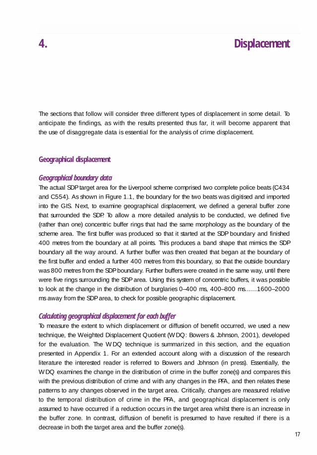
To calculate WDQ values for the entire buffer zone and for each of the five smaller bufferrings, it was necessary to calculate how many households were located in each buffer zone.This was established using information from Address Point5 and the GIS intersect command.The WDQ for the entire buffer zone was –1.4, indicating that there was evidence ofdisplacement and that the change in the buffer zone exceeded that in the SDP. Thus, furtherWDQs were computed for each of the buffer rings, these are shown in Figure 4.1. Theresults show that whilst there was, in general, evidence of geographical displacement therewas also a diffusion of benefit in the buffer ring contiguous with the SDP boundary. Thegreatest evidence of displacement was observed for the second buffer ring, the effect thendecreased in the subsequent rings, suggesting a possible distance decay effect.

18

5 The number of households was a proxy based upon the number of domestic postal delivery points, derived fromOrdnance Surveys Address Point data.

Figure 4.1: Weighted displacement quotients for the five buffer rings

Finally, we computed a weighted displacement quotient to examine the potentialgeographical displacement of burglary into the non-targeted area of the SDP. The valueobtained of -0.21 indicated that there was some evidence of displacement to this area butthat it was fairly limited.

Crime switch displacement

A further type of displacement that crime reduction schemes may cause is crime switchdisplacement which occurs when offenders swap from undertaking burglary to committingother types of crime in an area. Rather than focusing on all types of crime, for the purposesof illustration, this section will consider the effects of SDP activity on four types of acquisitivecrime: ‘theft from a person’, ‘theft of a car’, ‘theft from a car’ and the ‘unauthorised takingof a car’. These particular crimes were selected for the following reason. Felson and Clarke(1998) have argued that opportunity plays a role in causing all crime and that according torational choice theory (e.g. see Cornish & Clarke, 1989) the goal of criminal behaviour isto benefit the offender. Thus, it seems reasonable to suggest that following the removal ofopportunities for burglary, assuming that alternatives exist, offenders would seek to committhe most similar type of crime and select the next most similar targets. In terms of alternativetypes of crime that offenders may decide to commit, intuitively one would expect that thoselisted above would represent some of the most likely candidates.

The first approach adopted here to examine the effects of SDP activity on crime-switch was tosimply consider the changes in the rates of these crimes over time. One problem with calculatingrates for crimes such as car theft is that of selecting an appropriate denominator. For instance,whilst the selection of a denominator for (household) property crime is straightforward, this is notnecessarily the case for car crime. Ideally, one would use the number of cars that are, on

19

Wei

ghte

d D

ispl

acem

ent Q

uotie

nt 1.51

0.5

0-0.5

-1

-1.5

-2

-2.5

Buffer ring

1 2 3 4 5

average, parked in an area. However, although there is data concerned with the number ofcars owned by residents that reside within a particular Enumeration District (ED) there are anumber of problems with the use of this data here. The main concern with the use of such adenominator is that it is only available at the ED level, and the analyses conducted here areconcerned with effects at the sub-ED level (e.g. the SDP sub areas).

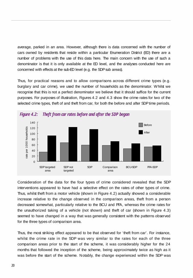
Thus, for practical reasons and to allow comparisons across different crime types (e.g.burglary and car crime), we used the number of households as the denominator. Whilst werecognise that this is not a perfect denominator we believe that it should suffice for the currentpurposes. For purposes of illustration, Figures 4.2 and 4.3 show the crime rates for two of theselected crime types, theft of and theft from car, for both the before and after SDP time periods.

Figure 4.2: Theft from car rates before and after the SDP began

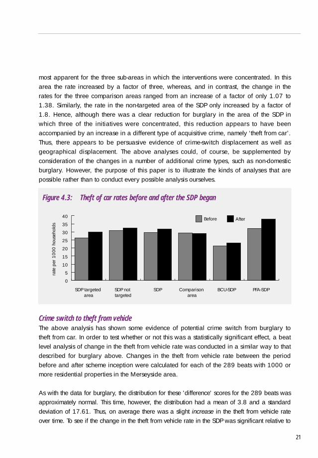
Consideration of the data for the four types of crime considered revealed that the SDPinterventions appeared to have had a selective effect on the rates of other types of crime.Thus, whilst theft from a motor vehicle (shown in Figure 4.2) actually showed a considerableincrease relative to the change observed in the comparison areas, theft from a persondecreased somewhat, particularly relative to the BCU and PFA, whereas the crime rates forthe unauthorized taking of a vehicle (not shown) and theft of car (shown in Figure 4.3)seemed to have changed in a way that was generally consistent with the patterns observedfor the three types of comparison area.

Thus, the most striking effect appeared to be that observed for ‘theft from car’. For instance,whilst the crime rate in the SDP was very similar to the rates for each of the threecomparison areas prior to the start of the scheme, it was considerably higher for the 24months that followed the inception of the scheme, being approximately twice as high as itwas before the start of the scheme. Notably, the change experienced within the SDP was

20

0

20

40

60

80

100

120

140Before

After

SDP targeted area

SDP not targeted

SDP Comparison area

BCU-SDP PFA-SDP

rate

per

100

0 ho

useh

olds

most apparent for the three sub-areas in which the interventions were concentrated. In thisarea the rate increased by a factor of three, whereas, and in contrast, the change in therates for the three comparison areas ranged from an increase of a factor of only 1.07 to1.38. Similarly, the rate in the non-targeted area of the SDP only increased by a factor of1.8. Hence, although there was a clear reduction for burglary in the area of the SDP inwhich three of the initiatives were concentrated, this reduction appears to have beenaccompanied by an increase in a different type of acquisitive crime, namely ‘theft from car’.Thus, there appears to be persuasive evidence of crime-switch displacement as well asgeographical displacement. The above analyses could, of course, be supplemented byconsideration of the changes in a number of additional crime types, such as non-domesticburglary. However, the purpose of this paper is to illustrate the kinds of analyses that arepossible rather than to conduct every possible analysis ourselves.

Figure 4.3: Theft of car rates before and after the SDP began

Crime switch to theft from vehicleThe above analysis has shown some evidence of potential crime switch from burglary totheft from car. In order to test whether or not this was a statistically significant effect, a beatlevel analysis of change in the theft from vehicle rate was conducted in a similar way to thatdescribed for burglary above. Changes in the theft from vehicle rate between the periodbefore and after scheme inception were calculated for each of the 289 beats with 1000 ormore residential properties in the Merseyside area.

As with the data for burglary, the distribution for these 'difference' scores for the 289 beats wasapproximately normal. This time, however, the distribution had a mean of 3.8 and a standarddeviation of 17.61. Thus, on average there was a slight increase in the theft from vehicle rateover time. To see if the change in the theft from vehicle rate in the SDP was significant relative to

21

Before After

SDP targeted area

SDP not targeted

SDP Comparison area

BCU-SDP PFA-SDP

rate

per

100

0 ho

useh

olds

0

5

10

15

20

25

30

35

40

the average change observed, z-scores were calculated for each beat. The two beats making upthe Liverpool SDP (beat codes C434 and C554) had z-scores of +1.71 and +3.43 respectively.Both of these z scores were significant at the 5 per cent level (one-tailed). In fact these two beatshad the 14th and 3rd highest positive z- scores for all 289 beats. This shows a very significantincrease in theft from vehicle for both the SDP beats. Interestingly, the z-score produced for thetargeted area of the SDP alone was +3.10, which is not as significant as beat C554.

For completeness, we also calculated a WDQ for this type of crime to examine the extent towhich crime-switch occurred. To do this, it was necessary to use a modified version of theWDQ formula (see Appendix 1). That is, rather than comparing the change in thedistribution of one type of crime in two different areas relative to the PFA, we wereconsidering the change in two types of crime in one area relative to the PFA. As with theabove analyses, the total number of households was used as a denominator to calculate thecrime rates for car crime. For the entire SDP the WDQ was –19.3 indicating that theincrease in the theft from car rate greatly exceeded the change in the burglary rate. For thetargeted area of the SDP, the WDQ was –0.87, demonstrating that the change in theburglary rate was similar to the increase in the theft from car rate. The results from the WDQthus also show that there was considerable evidence of crime switch.

A likely reason that may explain why crime switch appears to be most pronounced for this type ofcrime is the fact that theft from a motor vehicle is probably the next most similar crime to burglary.For instance, the skills required to commit these two types of crime are roughly equivalent, andthe types of goods acquired are likely to be similar both in terms of size and value, meaning thatthe offender should be able to sell the goods through existing channels/contacts.

In contrast, the other crime types, such as theft of an automobile, are likely to require differentskills, involve different risks, and possibly involve selling the goods through different or evennew contacts. Thus, from the rational choice perspective it would seem to make sense thatoffenders who perhaps specialise in committing burglaries would choose to steal from carsshould the availability of burglary opportunities become more limited or the risks increased.

However, a potentially puzzling aspect of the above results is that it can clearly be imputedthat both the WDQ and z-score analyses indicated that there was evidence of crime switchwithin the non-targeted area of the SDP. Since evidence suggests that offenders commitcrimes within close vicinity of their home address (e.g. Wiles and Costello, 2000), oneplausible reason for this may be that whilst offenders may commit burglaries in a fairlyanonymous fashion (that is, once inside a property the likelihood of being identified isrelatively minimal) the same is unlikely to be true for acquisitive car crime. Thus, from a

22

rational choice perspective, should crime-switch occur, it would make sense to commit carcrimes in areas that are just outside their own neighbourhood. In support of this, in a recentstudy, Wiles and Costello (2000) reported that offenders tend to commit car crimes (in thiscase, taking a vehicle without the owner’s consent) at a greater average distance from theirhome address than they do burglaries (the mean distances were 2.36 and 1.88 milesrespectively). A further possibility is concerned with offenders’ knowledge of the operationalboundary of the scheme and their understanding of the initiatives being implemented.Importantly, if offenders are simply aware that something is going on in the area, but arenot aware of the specifics of the intervention, then they may be more likely to avoidcommitting any type of crime in that area, meaning that should crime-switch occur it wouldperhaps be fairly prevalent in areas just outside the target area. Regardless of theunderlying cause of this effect, it seems plausible that this form of displacement may have ageographical as well as offence specific component to it.

Furthermore, whilst changes in the burglary rate were only statistically significant at the 5 percent level for the sub-areas, the changes in the crime rate for car crime were significant for allSDP areas (targeted, non-targeted and entire SDP). Thus, one may argue that since thechanges were always significant for car crime but not for burglary, it is difficult to attribute thechanges to crime-switch displacement. However, there are a number of reasons for believingthey are. First, there was evident selectivity in the patterns of change. Specifically, the actualchanges in crime rates, for both crime types, were greatest for the targeted area of the SDP,and the changes observed in each of the comparison areas (i.e. the comparison area, theBCU and the PFA) were almost non-existent or relatively small. Second, one reason why thechanges for car crime but not burglary were always significant may be due to a statisticalmeasurement or sensitivity issue. For example, to gain the same rewards as committing oneburglary, offenders may have to commit a number of car crimes. Thus, one burglaryprevented may lead to five or six incidents of theft from car. This means that although thechange in the burglary rate is small and difficult to detect, the change in the theft from carrate would clearly be substantial. One way of examining this issue is to consider the findingsfrom the 2000 British Crime Survey (Kershaw et al., 2000) concerned with the average costof goods stolen for these two types of crime. The results indicate that the cost of goods stolenfor an average burglary is £1,273, whereas the average yield for theft from car is £202.Thus, using a crude calculation, it would appear that offenders must commit at least six ‘theftfrom car’ offences to reap the same rewards as one burglary. Given this gearing ratio, wewould anticipate that if crime switch did occur even a small reduction in the burglary ratewould result in a fairly substantial increase in car crime. Thus, statistically it may be easier todetect changes in the latter even when changes in the former are less evident.

23

Heat threshold grid square analysisIt is possible to investigate the relationship between burglary and theft from vehicle in moredetail by looking at the spatial distribution of these crime types within the SDP area. In orderto do this, the SDP area was separated into 100 metre grid squares. Counts of burglary andtheft from car were then calculated for each of these squares for the two-year period beforeand the two-year period after the scheme's inception. These counts were then subtractedfrom each other to produce a measure of change for each crime type. These changes werethen mapped and the results are shown in Figures 4.4 (for burglary) and 4.5 (for theft fromvehicle). For both of the figures, squares were shaded using a heat threshold technique.Thus, red or brown squares indicate that the count of crime increased between the twoperiods, whereas those shaded in blue represent areas where there was a reduction.Squares that are shaded white are those in which the crime rate did not change betweenthe two periods. Figure 4.4 shows that, as expected, many of the squares within or nearbythe three targeted sub-areas show reductions in the count of burglary. In contrast, Figure 4.5shows that there were increases in theft from vehicle in these three sub-areas over the sameperiod of time.

24

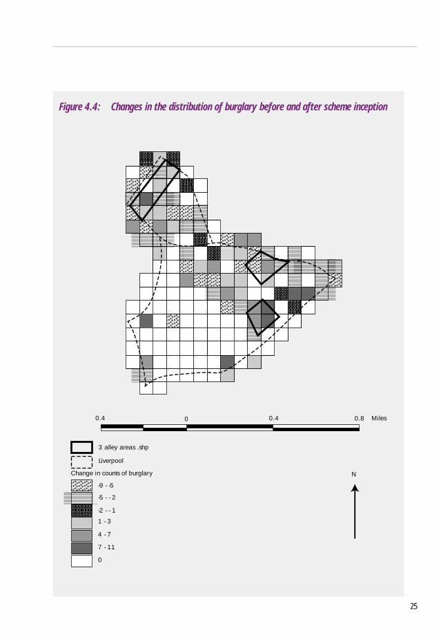
Figure 4.4: Changes in the distribution of burglary before and after scheme inception

25

3 alley areas .shp

Liverpool

Change in counts of burglary

-9 - -5

-5 - - 2

-2 - - 1

1 - 3

4 - 7

7 - 11

0

N

0.4 0 0.4 0.8 Miles

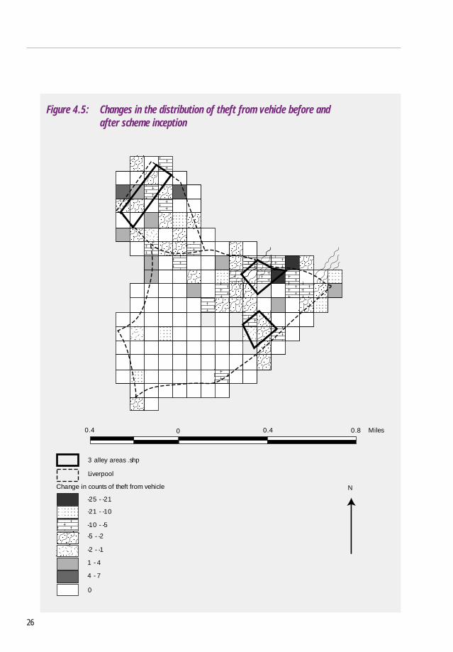
Figure 4.5: Changes in the distribution of theft from vehicle before and after scheme inception

26

Change in counts of theft from vehicle

3 alley areas .shp

Liverpool

-25 - -21

-21 - -10

-10 - -5

-5 - -2

-2 - -1

1 - 4

4 - 7

0

N

0.4 0 0.4 0.8 Miles

27

Target switch

The third type of displacement to be considered is that of target switch, which is said tohave occurred if offenders avoid properties that they may have otherwise targeted had theproperties not been subject to crime reduction activity. Furthermore, offenders instead selectthe next available properties within the scheme boundary. For instance, if it is likely thatnumber 10 on a particular road has received security upgrades as part of a targethardening scheme, but numbers 12–100 probably have not, then offenders may targetthese untreated properties instead.

Figure 4.6: Reduction in burglary rates for different groups of property

To examine this issue we calculated the number of burglaries that were committed atproperties that were and were not subject to crime reduction activity within the SDP. Nextwe computed the change in the rates for these different groups of properties over the beforeand after time periods. Rather than presenting the data as a simple percentage changefigure, we standardised the index of change as a function of the change observed for thehouses that were subject to crime reduction activity. Figure 4.6 shows the reduction in therate of burglary for six different types of area: the treated properties and the untreatedproperties located within the SDP sub areas, the remainder of the SDP boundary not subjectto situational crime reduction measures, the comparison area, the BCU and the PFA. As theindex of change was calculated as a function of the change observed in the treatedproperties, the index for these properties was set to –100(%). The Figure shows that the non-targeted properties in the near vicinity of those that were treated (i.e. those within the threesmaller sub-areas shown in Figure 1) experienced a large percentage reduction in theiroverall burglary rate relative to the treated properties. In fact, these properties saw almostas much of a decrease (95 per cent) as the treated properties themselves. There was also aslight reduction in the non-targeted part of the SDP (those outside the three sub-areas inFigure 1.1) but this was not on the scale of the non-targeted properties within the sub-areas.

6040200

-20-40-60-80

-100-120

PFA - SDPBCU-SDPComparison area

Non targeted part of SDP

Non-target hardened

properties in targeted area

Targethardened

properties in targeted area

In addition, this drop was not as large as that seen in the remainder of the PFA (PFA–SDP).The changes in both the comparison area and the BCU were actually positive (to differingdegrees), indicating that relative to the treated properties there was an actual increase inrisk in these two areas, rather than the slower decrease observed in the other areas.

It therefore appears from the graph that the non-targeted properties within the sub-areasbenefited from the fact that they were located nearby to houses that had received treatment.This represents evidence of diffusion of benefit, and suggests that the possibility of targetswitch to other properties within the intervention areas is unlikely. It also appears that thediffusion of benefit is fairly localised in its nature because there was far less of a (relative)reduction in the burglary rate in the part of the SDP outside the three sub-areas. This is likelyto be demonstrating a spatial proximity effect, suggesting that offenders are aware thatcrime reduction activity is happening in the area but are not sure which specific houseshave been targeted and therefore avoid all houses in the immediate area of the intervention.This has clear implications for the planning of crime reduction initiatives, particularly formaximising the effects of limited resources.

28

29

5. Effectiveness of interventions

Measuring the effects of a single intervention

This section considers the effectiveness of individual interventions by examining the changesin the burglary rate for protected properties over time. It begins by using information on theactual location of target-hardened properties within the Liverpool SDP area to illustrate themethodology developed and then proceeds to consider the effectiveness of the otherinterventions. The address of each property that received target-hardening was supplied bythe SDP team. These were then allocated easting and northing co-ordinates using AddressPoint information (a geographical database). Briefly, the addresses were cleaned andrewritten in Address Point structure and then matched with the Address Point data in a GIS,using the unique combination of house number and postcode, fields that were common toboth files. These data were then mapped using a GIS. Visual inspection of the map revealedthat the target-hardened properties were almost exclusively located within the three sub-areas of the SDP.

In order to evaluate the effectiveness of target hardening in reducing burglary, theinformation on the location of target-hardened properties needed to be cross-referenced withinformation on burglaries occurring at these addresses. The most accurate method ofachieving this was by restructuring the burglary data in the same format as the targethardening information. A FORTRAN program was therefore produced that re-formattedburglaries into Address Point format. Then, using address-matching software produced forthe evaluation, the recorded crime and target-hardening databases were searched and anyburglaries that had occurred in target-hardened properties were identified. Each of theburglaries had date information attached to them, which enabled a count to be produced ofthe number of burglaries against target-hardened properties that had occurred before andafter inception of the Liverpool SDP scheme.

Table 5.1 summarises the raw count of incidents both before and after the SDP becameactive (simply searching for incidents before and after 1st April 1999). Although resultsshown in Table 5.1 are produced on an individual level, to preserve anonymity theinformation was aggregated to give the total number of times that all target hardenedproperties were victimised before and after locks were fitted.

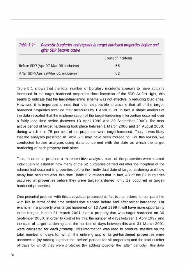
Table 5.1: Domestic burglaries and repeats in target hardened properties before andafter SDP became active

Count of incidents

Before SDP (Apr 97-Mar 99 inclusive) 55

After SDP (Apr 99-Mar 01 inclusive) 62

Table 5.1 shows that the total number of burglary incidents appears to have actuallyincreased in the target hardened properties since inception of the SDP. At first sight, thisseems to indicate that the target-hardening scheme was not effective in reducing burglaries.However, it is important to note that it is not possible to assume that all of the target-hardened properties received their measures by 1 April 1999. In fact, a simple analysis ofthe data revealed that the implementation of the target-hardening intervention occurred overa fairly long time period (between 13 April 1999 and 30 September 2000). The mostactive period of target hardening took place between 1 March 2000 and 14 August 2000,during which time 75 per cent of the properties were target-hardened. Thus, it was likelythat the analyses presented in Table 5.1 may have been misleading. For this reason, weconducted further analyses using data concerned with the date on which the targethardening of each property took place.

Thus, in order to produce a more sensitive analysis, each of the properties were trackedindividually to establish how many of the 62 burglaries carried out after the inception of thescheme had occurred in properties before their individual date of target hardening and howmany had occurred after this date. Table 5.2 reveals that in fact, 43 of the 62 burglariesoccurred at properties before they were target-hardened; only 19 occurred in target-hardened properties.

One potential problem with this analysis as presented so far, is that it does not compare likewith like in terms of the time periods that elapsed before and after target hardening. Forexample, if a property was target hardened on 13 April 1999 it will have more opportunityto be burgled before 31 March 2001 than a property that was target hardened on 30September 2000. In order to control for this, the number of days between 1 April 1997 andthe date of target hardening and the number of days between this and 31 March 2001were calculated for each property. This information was used to produce statistics on thetotal number of days for which the entire group of target-hardened properties wereunprotected (by adding together the ‘before’ periods for all properties) and the total numberof days for which they were protected (by adding together the ‘after’ periods). This data

30

31

was then used as a denominator to produce a standardised rate which controlled for theperiod of victimisation opportunity for each household. These ‘opportunity dependentincident counts’ are shown in Table 5.2. The results demonstrate that, even when differencesin victimisation opportunity have been accounted for, there is a difference in the number ofincidents happening before and after target hardening. In fact, target-hardened householdswere at almost half of the risk of unprotected houses in the same area. This is a particularlyimportant finding given that research consistently demonstrates that victimisation predictsfuture risk (e.g. see Pease, 1998), and the fact that part of the selection criteria for targethardening included identifying previously victimised households. Thus, ordinarily the target-hardened properties would be precisely those that would be expected to be at a heightenedrather than reduced risk. These results suggest that the target hardening intervention hadbeen successful.

Table 5.2: Revised table examining burglaries that happened after inception date inrelation to their individual target hardening date

Count of incidents Number of days for all Opportunity dependenttarget hardened properties count of incidents

Before TH 98 394665 24.83*

After TH 19 135285 14.04*

*To ease interpretation these are scaled up by 100,000

A further extension to this methodology is the translation of the information presented inTable 5.2 into a quantification of the outcome of the particular intervention from the pointof view of the number of burglaries reduced or prevented by the measures taken. Table 5.3shows the steps taken to calculate this outcome. As demonstrated above, the first stage wasto produce opportunity-dependent counts of incidents. In this case, the counts have beenscaled to relate to a ‘virtual year’ for the properties concerned, which produces slightlydifferent results from those in Table 5.2, which used a different scaling factor. This ‘virtualyear’ is calculated by multiplying the number of target hardened properties by the numberof days in a year. For the 363 target hardened properties therefore, 132495 days makesup a virtual year. This scaling was undertaken because it was sensible to have ameaningful period of analysis for the production of outcomes. In order to produceoutcomes, the number of burglaries occurring after target hardening required comparisonwith an expected rate. An expected rate was produced by taking into account changes inthe wider PFA over time. Therefore;

(Note that the area used is the Police Force Area minus the Basic Command Unit whichcontains the SDP in order to avoid confounding this ratio by including areas possiblyaffected by the activity of the SDP scheme).

Table 5.3: Outcomes for target hardening scheme

Count of Number of Opportunity Average Expected no Noincidents days for all dependent PFA-BCU of burglaries burglaries

target count of count for after preventedhardened incidents quarters by schemeproperties before and

after targethardening

Before 98 394665 32.90* 2510THAfter 19 135285 18.61* 2407 31.55 12.94TH

* These are for virtual years (132,495 days for 363 households)

This expected rate therefore reflects what we might expect the incident count to be if nothingoccurred in the SDP. That is, if the proportion of burglaries committed in the PFA that wereconcentrated in the SDP remained stable over time. In order to calculate the outcome (or thenumber of burglaries saved by the scheme) in Table 5.3 the observed number of burglariesoccurring after target hardening was simply subtracted from the expected number. Table 5.3therefore shows a saving of 13 burglaries in one (virtual) year for the 363 propertiesinvolved in the intervention.

Measuring the effects of multiple interventions

So far in this section, the analysis of outcomes at the individual level has only investigatedthe effect of target hardening on levels of burglary. The reality is that other initiatives, suchas smartwater and alleygating may also have an effect at this level. Furthermore, some ofthe households that had been target-hardened were also protected by smartwater and/or

32

Average PFA count before target hardening

Average PFA count after target hardening

number of burglariesin properties before target hardening

Expected burglaries = x

alleygating. In order to try to separate out the effects of these interventions, a database wasproduced that contained all of the households that had been involved in at least one ofthese three interventions. For each household, there was a dummy variable that indicatedwhether the property had been target hardened, smart-watered or alleygated and dataconcerned with the dates on which these measures had been installed.

Using the address matching software, this database was then matched against individualburglary data for the period between 1 April 1997 and 31 March 2001. In a similarmethod to that described above, the date of each burglary was compared with the date ofinstallation of the measures taken at each property. Table 5.4 below shows the results of thisanalysis. The table shows that overall there were 500 individual households that had beentreated by at least one intervention. The most common situation was that properties weretarget hardened without any other treatment (168 properties). There was also a substantialamount of cases in which properties received both target hardening and smartwater (136properties). Less common were individual properties that had received all three interventions(31 properties), alleygating and target hardening (28 properties) or alleygating andsmartwater (7 properties). The number of burglaries saved by each of the combinations oftreatment was calculated using the opportunity dependent rate method described above. Asabove, these outcomes were calculated for a ‘virtual year’ for that number of households.For example, for alleygating there were 76 treated properties, which meant that a virtualyear would be equivalent to 76*365 = 27740 days. The savings shown in Table 5.4should therefore be taken as being for a virtual year for the particular number of propertiesreceiving that combination of interventions.

By adding up the outcomes, it can be seen that overall across the different combinations ofinterventions, there was a saving of approximately 12 burglaries. It is interesting tocompare the different savings across the different types of treatment. It appears from Table5.4 that undertaking target hardening, either on its own or in combination with one or moreother intervention, appears to be a particularly effective treatment. In fact, according to thefigures target hardening on its own appears to be more effective than using it incombination with other measures. However, this may be due to the fact that morehouseholds received target hardening alone than those using combinations of measures. Thetwo combinations of interventions that appeared least effective was smartwater alone,which showed an increase of 2.49 burglaries over the expected rate, and alleygating andSmartwater, which showed no change, although the number of cases in the latter category(7 properties) was too small for reliable analysis.

33

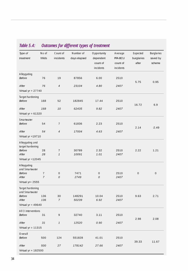
Table 5.4: Outcomes for different types of treatment

Type of No of Count of Number of Opportunity Average Expected Burglaries

treatment hhlds incidents days elapsed dependent PFA-BCU burglaries saved by

count of count of after scheme

incidents incidents

AlleygatingBefore 76 19 87856 6.00 2510

5.75 0.95After 76 4 23104 4.80 2407

Virtual yr = 27740

Target hardeningBefore 168 52 182845 17.44 2510

16.72 6.9After 168 10 62435 9.82 2407

Virtual yr = 61320

SmartwaterBefore 54 7 61836 2.23 2510

2.14 -2.49After 54 4 17004 4.63 2407

Virtual yr =19710

Alleygating and target hardeningBefore 28 7 30789 2.32 2510 2.22 1.21After 28 1 10091 1.01 2407

Virtual yr =12045

Alleygatingand SmartwaterBefore 7 0 7471 0 2510 0 0After 7 0 2749 0 2407

Virtual yr= 2555

Target hardening and SmartwaterBefore 136 30 148291 10.04 2510 9.63 2.71After 136 7 50239 6.92 2407

Virtual yr = 49640

All 3 interventionsBefore 31 9 32740 3.11 2510

2.98 2.08After 31 1 12520 0.90 2407

Virtual yr = 11315

OverallBefore 500 124 551828 41.01 2510

39.33 11.67After 500 27 178142 27.66 2407

Virtual yr = 182500

34

35

6. The influence of other initiatives

An important final consideration in assessing the impact of the RBI is the role played byother crime reduction and regeneration initiatives that are operating in the area. The SDPtarget area was originally chosen so that it would not co-incide with the European UnionObjective 1 areas. In doing so, it was ensured that the SDP did not overlap with areas inwhich the Safer Merseyside Partnership, a nine-year crime reduction programme, wasoperational. However, there is the possibility that other crime reduction efforts, such as thoseof Merseyside Police Force and those laid out in the Crime and Disorder strategies for thedistrict of Liverpool, might have some impact on burglary rates in the target area. For thisreason, information concerning such schemes was collected. Some of these had acommunity safety element and their geographical boundary covered both the Liverpool andMerseyside areas. Thus, it is possible that some of these projects could have had a potentialeffect on the crime rates within and nearby the Liverpool SDP area. For instance, a HealthAction Zone parenting support project and a youth exclusion project had a city-wide remit,and hence both operated in the SDP area. Furthermore, a Streetsafe police initiative and theDingle Community Regeneration team project's CCTV initiative also operate in the SDParea. All the schemes mentioned above were implemented at least partially within thetimescale of the Liverpool SDP. It is difficult to assess the effect of these schemes on crimerates within the SDP area without having specific information on the inputs and outputs forthese schemes. However, since all the schemes mentioned above were implemented acrosswide areas of the city of Liverpool, it is reasonable to assume that the BCU, the comparisonarea and the buffer zones that have been used in the analyses described here would allhave been affected by these initiatives. This means that to a certain degree the influence ofother initiatives was controlled for in the analyses. It would be more problematic if any ofthe other crime reduction initiatives had focused on a far smaller geographical area ofwhich the SDP (but not the comparison areas, or vice versa) was a part.

37

7. Concluding remarks

This paper has illustrated the power of disaggregate data analysis in the evaluation of theeffectiveness of burglary reduction schemes, and has shown that the use of aggregate levelinformation alone may produce misleading results. It has also presented new methods forquantifying the outcomes of such schemes. These methods include new techniques formeasuring changes in the burglary rate, assigning statistical significance to such changes,assessing the degree to which action causes crime displacement and a way of isolatingburglary reduction outcomes that can be attributable to specific interventions undertaken.

The authors would like to emphasise that it should be possible to use techniques such as thosedescribed above to assess both the impact of burglary reduction schemes in other areas,and, in some cases, the impact of other crime reduction schemes. For instance, similartechniques could be used to assess the statistical significance of schemes aimed at reducingcar crime or reducing crime through CCTV surveillance. The ability to undertake any suchventures relies on the availability of accurate, individual level recorded crime information.

Considering the scheme used to illustrate the techniques presented here, whilst the purposeof this paper was to focus on the methods developed, some discussion of the scheme itselfand relevant policy implications is clearly warranted. However, before discussing theeffectiveness of the scheme it is necessary to comment on the implementation of theinterventions. Considering the target hardening and property marking initiatives, these weresuccessfully implemented within the time period studied. And, analyses of the dates onwhich target-hardening surveys took place indicated that the majority did so immediatelyafter a burglary, illustrating that the targeting strategy employed was efficient. In addition,since research (see Pease, 1998) illustrates that the majority of repeat incidents of burglaryoccur swiftly, the approach adopted would have ensured that properties were protectedduring the period that they were most vulnerable. Thus, the effectiveness of the scheme wasnot compromised by an inappropriate targeting strategy.

In contrast, the alley-gating scheme was not fully realised during the evaluation period andthis will undoubtedly have had an impact on the effectiveness of the scheme. As notedabove, because of legal reasons only ten of the intended 69 gates were fitted during theperiod considered. These gates secured one block of 125 houses. Problems were alsoexperienced by the offender-based scheme, as follows. First, due to initial problems inrecruiting a police officer, the scheme did not become operational until January 2000.

Second, for the above period, only six offenders had participated in the scheme. Third, all ofthe offenders who took part in the scheme had recently been released from prison on licence.Thus, it is plausible that the offenders operating in the target area for both the pre- and post-implementation periods did not actually take part in the scheme. Thus, it is difficult to see howthe scheme could have had an effect on the behaviour of those offenders who wereresponsible for the crime rate in the target area within the time period studied. Finally, forthese and other reasons, it is worth noting that behaviour modification programmes may wellrequire a much longer period than situational crime reduction initiatives to produce reliableand/or sustainable effects, and thus it is our opinion that whilst this intervention may haveproduced reliable results in terms of changing the behaviour of the offenders who took part inthe scheme, it is unlikely to have impacted upon the crime rate in the SDP at this stage.

Notwithstanding these initial implementation problems, the analyses presented abovesuggest that, to some extent at least, the scheme was successful in reducing the burglary ratein the targeted area. Although the reduction observed across the entire SDP was statisticallynon-significant, the change apparent in the three sub-areas in which the situational crimereduction measures were geographically focused clearly was. In terms of repeatvictimisation, there was a clear reduction across the entire SDP, although this again wasmost evident in the three targeted sub-areas.

Considering the time period during which the scheme appeared to be most effective, perhapsnot surprisingly this appears to have occurred during the most intensive implementation phaseof the scheme (see Figure 2.3). However, the crime rate rose steeply in the final quarter of theevaluation period. Assuming that this was a reliable increase, this may suggest twopossibilities regarding the mechanism through which the scheme had an effect. First, it ispossible that the effect was simply not sustainable and that offenders discovered methods ofcircumventing the measures taken. Alternatively, it is possible that the change in the SDP mayhave been attributable to a realisation on the part of offenders that ‘something’ was going on(or was about to) in the target area which would affect the risk of being caught, an effectgenerally referred to as the ‘Hawthorne effect’ (see Mayo, 1933; see also Smith et al,forthcoming). In this latter case, the reduction observed would be assumed to result from achange in offenders’ perceptions of the risks involved in committing crimes in the area, ratherthan because of the actual difficulty in gaining access to the protected properties. In supportof this possibility, in a forthcoming book chapter that considers the role of the Hawthorneeffect in crime reduction schemes, Smith et al report that of the 52 evaluations considered, 40per cent showed evidence of a reduction in the crime rate in advance of the physicalimplementation of the interventions, an effect that Smith et al refer to as an anticipatorybenefit. Unfortunately, it is beyond the scope of the current paper to determine which of the

38

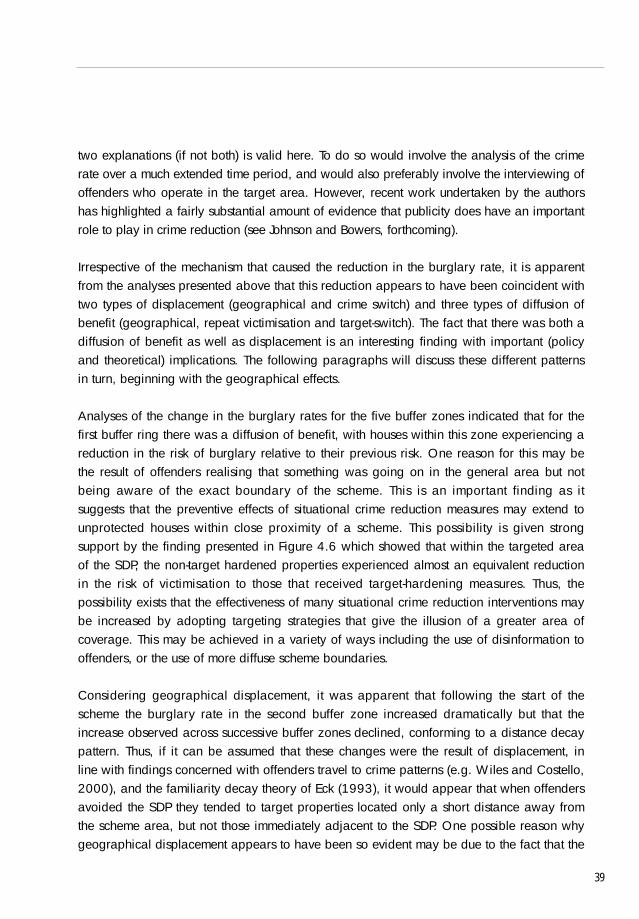
two explanations (if not both) is valid here. To do so would involve the analysis of the crimerate over a much extended time period, and would also preferably involve the interviewing ofoffenders who operate in the target area. However, recent work undertaken by the authorshas highlighted a fairly substantial amount of evidence that publicity does have an importantrole to play in crime reduction (see Johnson and Bowers, forthcoming).

Irrespective of the mechanism that caused the reduction in the burglary rate, it is apparentfrom the analyses presented above that this reduction appears to have been coincident withtwo types of displacement (geographical and crime switch) and three types of diffusion ofbenefit (geographical, repeat victimisation and target-switch). The fact that there was both adiffusion of benefit as well as displacement is an interesting finding with important (policyand theoretical) implications. The following paragraphs will discuss these different patternsin turn, beginning with the geographical effects.

Analyses of the change in the burglary rates for the five buffer zones indicated that for thefirst buffer ring there was a diffusion of benefit, with houses within this zone experiencing areduction in the risk of burglary relative to their previous risk. One reason for this may bethe result of offenders realising that something was going on in the general area but notbeing aware of the exact boundary of the scheme. This is an important finding as itsuggests that the preventive effects of situational crime reduction measures may extend tounprotected houses within close proximity of a scheme. This possibility is given strongsupport by the finding presented in Figure 4.6 which showed that within the targeted areaof the SDP, the non-target hardened properties experienced almost an equivalent reductionin the risk of victimisation to those that received target-hardening measures. Thus, thepossibility exists that the effectiveness of many situational crime reduction interventions maybe increased by adopting targeting strategies that give the illusion of a greater area ofcoverage. This may be achieved in a variety of ways including the use of disinformation tooffenders, or the use of more diffuse scheme boundaries.

Considering geographical displacement, it was apparent that following the start of thescheme the burglary rate in the second buffer zone increased dramatically but that theincrease observed across successive buffer zones declined, conforming to a distance decaypattern. Thus, if it can be assumed that these changes were the result of displacement, inline with findings concerned with offenders travel to crime patterns (e.g. Wiles and Costello,2000), and the familiarity decay theory of Eck (1993), it would appear that when offendersavoided the SDP they tended to target properties located only a short distance away fromthe scheme area, but not those immediately adjacent to the SDP. One possible reason whygeographical displacement appears to have been so evident may be due to the fact that the

39

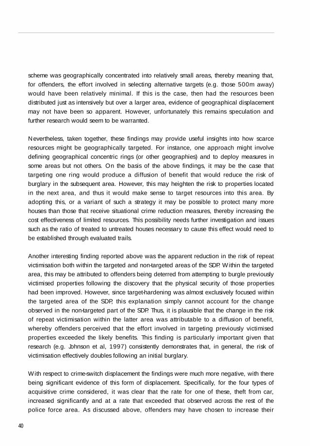
scheme was geographically concentrated into relatively small areas, thereby meaning that,for offenders, the effort involved in selecting alternative targets (e.g. those 500m away)would have been relatively minimal. If this is the case, then had the resources beendistributed just as intensively but over a larger area, evidence of geographical displacementmay not have been so apparent. However, unfortunately this remains speculation andfurther research would seem to be warranted.

Nevertheless, taken together, these findings may provide useful insights into how scarceresources might be geographically targeted. For instance, one approach might involvedefining geographical concentric rings (or other geographies) and to deploy measures insome areas but not others. On the basis of the above findings, it may be the case thattargeting one ring would produce a diffusion of benefit that would reduce the risk ofburglary in the subsequent area. However, this may heighten the risk to properties locatedin the next area, and thus it would make sense to target resources into this area. Byadopting this, or a variant of such a strategy it may be possible to protect many morehouses than those that receive situational crime reduction measures, thereby increasing thecost effectiveness of limited resources. This possibility needs further investigation and issuessuch as the ratio of treated to untreated houses necessary to cause this effect would need tobe established through evaluated trails.

Another interesting finding reported above was the apparent reduction in the risk of repeatvictimisation both within the targeted and non-targeted areas of the SDP. Within the targetedarea, this may be attributed to offenders being deterred from attempting to burgle previouslyvictimised properties following the discovery that the physical security of those propertieshad been improved. However, since target-hardening was almost exclusively focused withinthe targeted area of the SDP, this explanation simply cannot account for the changeobserved in the non-targeted part of the SDP. Thus, it is plausible that the change in the riskof repeat victimisation within the latter area was attributable to a diffusion of benefit,whereby offenders perceived that the effort involved in targeting previously victimisedproperties exceeded the likely benefits. This finding is particularly important given thatresearch (e.g. Johnson et al, 1997) consistently demonstrates that, in general, the risk ofvictimisation effectively doubles following an initial burglary.

With respect to crime-switch displacement the findings were much more negative, with therebeing significant evidence of this form of displacement. Specifically, for the four types ofacquisitive crime considered, it was clear that the rate for one of these, theft from car,increased significantly and at a rate that exceeded that observed across the rest of thepolice force area. As discussed above, offenders may have chosen to increase their

40

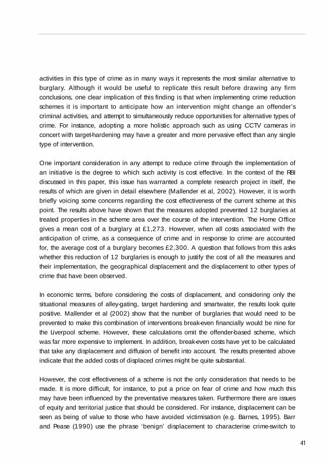
activities in this type of crime as in many ways it represents the most similar alternative toburglary. Although it would be useful to replicate this result before drawing any firmconclusions, one clear implication of this finding is that when implementing crime reductionschemes it is important to anticipate how an intervention might change an offender’scriminal activities, and attempt to simultaneously reduce opportunities for alternative types ofcrime. For instance, adopting a more holistic approach such as using CCTV cameras inconcert with target-hardening may have a greater and more pervasive effect than any singletype of intervention.

One important consideration in any attempt to reduce crime through the implementation ofan initiative is the degree to which such activity is cost effective. In the context of the RBIdiscussed in this paper, this issue has warranted a complete research project in itself, theresults of which are given in detail elsewhere (Mallender et al, 2002). However, it is worthbriefly voicing some concerns regarding the cost effectiveness of the current scheme at thispoint. The results above have shown that the measures adopted prevented 12 burglaries attreated properties in the scheme area over the course of the intervention. The Home Officegives a mean cost of a burglary at £1,273. However, when all costs associated with theanticipation of crime, as a consequence of crime and in response to crime are accountedfor, the average cost of a burglary becomes £2,300. A question that follows from this askswhether this reduction of 12 burglaries is enough to justify the cost of all the measures andtheir implementation, the geographical displacement and the displacement to other types ofcrime that have been observed.

In economic terms, before considering the costs of displacement, and considering only thesituational measures of alley-gating, target hardening and smartwater, the results look quitepositive. Mallender et al (2002) show that the number of burglaries that would need to beprevented to make this combination of interventions break-even financially would be nine forthe Liverpool scheme. However, these calculations omit the offender-based scheme, whichwas far more expensive to implement. In addition, break-even costs have yet to be calculatedthat take any displacement and diffusion of benefit into account. The results presented aboveindicate that the added costs of displaced crimes might be quite substantial.

However, the cost effectiveness of a scheme is not the only consideration that needs to bemade. It is more difficult, for instance, to put a price on fear of crime and how much thismay have been influenced by the preventative measures taken. Furthermore there are issuesof equity and territorial justice that should be considered. For instance, displacement can beseen as being of value to those who have avoided victimisation (e.g. Barnes, 1995). Barrand Pease (1990) use the phrase ‘benign’ displacement to characterise crime-switch to

41

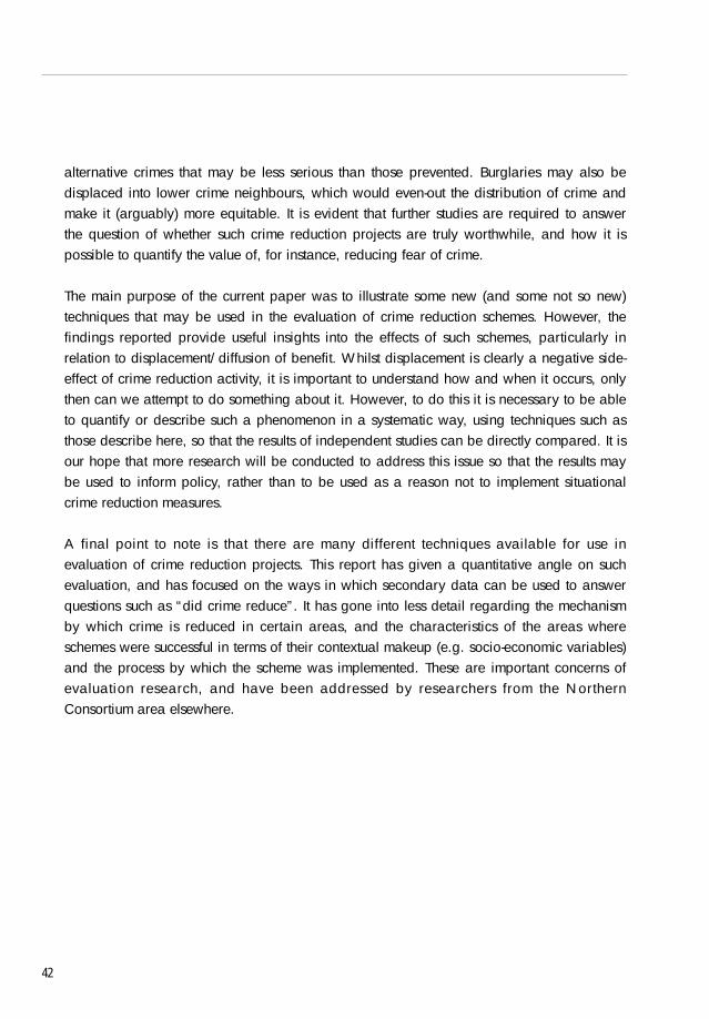
alternative crimes that may be less serious than those prevented. Burglaries may also bedisplaced into lower crime neighbours, which would even-out the distribution of crime andmake it (arguably) more equitable. It is evident that further studies are required to answerthe question of whether such crime reduction projects are truly worthwhile, and how it ispossible to quantify the value of, for instance, reducing fear of crime.

The main purpose of the current paper was to illustrate some new (and some not so new)techniques that may be used in the evaluation of crime reduction schemes. However, thefindings reported provide useful insights into the effects of such schemes, particularly inrelation to displacement/diffusion of benefit. Whilst displacement is clearly a negative side-effect of crime reduction activity, it is important to understand how and when it occurs, onlythen can we attempt to do something about it. However, to do this it is necessary to be ableto quantify or describe such a phenomenon in a systematic way, using techniques such asthose describe here, so that the results of independent studies can be directly compared. It isour hope that more research will be conducted to address this issue so that the results maybe used to inform policy, rather than to be used as a reason not to implement situationalcrime reduction measures.

A final point to note is that there are many different techniques available for use inevaluation of crime reduction projects. This report has given a quantitative angle on suchevaluation, and has focused on the ways in which secondary data can be used to answerquestions such as “did crime reduce”. It has gone into less detail regarding the mechanismby which crime is reduced in certain areas, and the characteristics of the areas whereschemes were successful in terms of their contextual makeup (e.g. socio-economic variables)and the process by which the scheme was implemented. These are important concerns ofevaluation research, and have been addressed by researchers from the NorthernConsortium area elsewhere.

42

Appendix 1 Formula for the weighted displacement quotient

In a forthcoming paper (Bowers and Johnson, in press) we review the extant literatureconcerned with the displacement of crime and diffusion of benefits. In particular, we discussthe techniques that have been used to measure these phenomenon and the potentialproblems associated with these methods. Consequently, we present a new standardizedtechnique, the weighted displacement quotient (WDQ), which can be used to measureeither phenomena. The rationale and assumptions underlying this technique are presented infull in the forthcoming paper. However, to enable evaluators to use this technique now, theequation for the WDQ is presented below.

Formula for the weighted displacement quotient

The equation used for comparing the rate in the buffer to the police force area is given by:

Rate in (buffer zone)/rate in (PFA- buffer zone - SDP) (1.1)

The index is then weighted using a measure that compares the rate in the target area to thatin the police force area:

Rate in SDP/Rate in (PFA-buffer zone-SDP) (1.2)

Giving a weighted measure of:

Rate in (buffer zone)/rate in (PFA-buffer -SDP) (1.3)Rate in SDP/Rate in (PFA-buffer zone-SDP)

However, in its current form this index only looks at the differing proportions in the variousareas at one time point. And, consequently, as the term ‘rate in (PFA-buffer zone-SDP)’appears in both the numerator and denominator components of the equation for the sametime point, it cancels itself out. In order to detect displacement, the situation after the crimereduction scheme became active needs to be compared with the situation before. Ifdisplacement has occurred we would expect the numerator of the equation above toincrease over time and the denominator to decrease – in other words for the scheme to be

43

successful and the proportion of crime committed in the buffer zone to increase. If thescheme is not successful, theoretically we would not expect to observe any evidence ofdisplacement or diffusion of benefit, and hence it is unlikely that any change in the bufferzone can be attributed to activity within the scheme. Therefore, if there is no indication of areduction in crime within the SDP it is inappropriate to attempt to interpret any changes interms of potential displacement or diffusion of benefit.

In order to look at changes in proportions over time the weighted displacement quotientcompares the situation after implementation (t1) with the situation before (t0) using thefollowing formula:

Note that in this formulation of the equation, the term ‘(PFA-buffer zone-SDP)’ no longercancels itself out as it did in equation 1.3.

Further details regarding the WDQ technique may be obtained from the authors, email:[email protected] or [email protected].

44

{Rate in (buffer)/rate in (PFA-buffer-SDP)}t1- {Rate in (buffer)/rate in (PFA-buffer-SDP)}t0

{Rate in SDP/Rate in (PFA-buffer-SDP)}t1 - {Rate in SDP/Rate in (PFA-buffer-SDP)}t0(1.4)

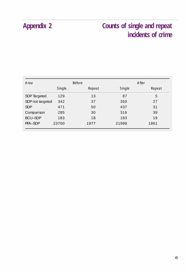
Appendix 2 Counts of single and repeat incidents of crime

Area Before AfterSingle Repeat Single Repeat

SDP Targeted 129 13 87 5SDP not targeted 342 37 350 27SDP 471 50 437 31Comparison 285 30 316 39BCU–SDP 183 18 183 19PFA–SDP 23700 1977 21998 1861

45

47

References

Anderson, D., Chenery, S. and Pease, K. (1995): Biting Back: Tackling RepeatBurglary and Car Crime, Crime Detection and Prevention Series Paper 58. London: HomeOffice

Barnes, G. (1995) Defining and optimising displacement. In Eck, J. and Weisburd, D.(eds) Crime and Place. Crime Prevention Studies Volume 4, 95–114. Monsey, NY: CriminalJustice Press.

Barr, R. & Pease, K. (1990) Crime placement, displacement and deflection. Crime andJustice: A Review of the Research. 12, 277–318.

Bennett, T.H. and Durie, L. (1999) Preventing Residential Burglary in Cambridge.Crime Detection and Prevention Series, Paper 182. Police Research Group. London: HomeOffice.

Bowers, K.J. & Johnson, S.D. (2001) Measuring the Geographical Displacement ofCrime. Submitted to the Journal of Quantitative Criminology.

Cornish, D.B. & Clarke, R. V. (1989) Crime specialization, crime displacement andrational choice theory. In Wegner, H., Losel, F., and Haisch, J. (eds): Criminal Behaviourand the Justice System: Psychological perspectives. New York: Springer-Verlag:

Eck, J. (1993) The threat of crime displacement, Criminal Justice Abstracts, 25, 527–546.

Felson, M., & Clarke, R.V. (1998) Opportunity makes the thief: practical theory forcrime prevention, Police Research Series, Paper 98. London: Home Office.

Hirschfield, A. & Bowers, K. (1997) ‘The development of a social, demographic andland use profiler for areas of high crime’, British Journal of Criminology 37 (1),103–120.

Johnson, S.D. and Bowers, K (forthcoming) Opportunity is in the eye of the beholder:The role of publicity in crime prevention. Submitted to the Crime Reduction Research Series,London: Home Office,

Johnson, S.D, Bowers, K., Hirschfield, A., & Brown, P. (1996) A program for theidentification of repeat victimisation, Urban Research and Policy Evaluation RegionalResearch Laboratory: Software Note, 8, 1–12.

Johnson, S.D., Bowers, K.J. and Hirschfield, A.F.G. (1997): New insights into thespatial and temporal distribution of repeat victimisation, British Journal of Criminology,37(2), pp. 224–241.

Johnson, S.D., Bowers, K.J., Young, C.A., & Hirschfield, A.F.G. (2001).Uncovering the true picture: evaluating crime reduction initiatives using disaggregate crimedata. Crime Prevention and Community Safety: An International Journal (in press).

Johnson, S.D., & Loxley, C. (2001). Installing alley-gates: practical lessons fromburglary prevention projects. Home Office Crime Reduction Research Series, 2(1). London:Home Office.

Kershaw, C., Budd, T., Kinshott, G., Mattinson, J., Mayhew, P. and Myhill, A.(2000) The 2000 British Crime Survey: England and Wales. Home Office Statistical Bulletin18/00. London: Home Office.

Mallender, J., Richman, A. and Kingsnorth, R. (2002) Reducing Burglary Initiative:Evaluating Costs and Benefits Liverpool Strategic Development Project: A Case Study

Mayo, E. (1933). The Human Problems of an Industrial Civilisation. New York: Macmillan.

Pease, K. (1998) Repeat victimisation: Taking stock. Crime Detection and PreventionSeries, Paper 90. London: Home Office.

Smith, M.J., Clarke, R.V., & Pease, K. (forthcoming) Anticipatory benefit in crimeprevention. In Tilley, N. (ed.) Crime Prevention Studies 14.

Tilley, N., Pease, K., Hough, M. and Brown, R. (1999) Burglary prevention: earlylessons from the Crime Reduction Programme. Crime Reduction Research Series, Paper 1.London: Home Office.

Wiles, P. and Costello, A. (2000) ‘The Road to Nowhere’: The evidence for travellingcriminals. Home Office Research Study No 207. London: Home Office.

48

50

RDS Publications

Requests for Publications

Copies of our publications and a list of those currently available may be obtained from:

Home OfficeResearch, Development and Statistics DirectorateCommunication Development UnitRoom 264, Home Office50 Queen Anne’s GateLondon SW1H 9ATTelephone: 020 7273 2084 (answerphone outside of office hours)Facsimile: 020 7222 0211E-mail: [email protected]

alternatively

why not visit the RDS web-site atInternet: http://www.homeoffice.gov.uk/rds/index.htm

where many of our publications are available to be read on screen or downloaded forprinting.

Pushing back the boundaries:new techniques forassessing the impactof burglary schemes - summary

summary to Home Office Online Report 24/03

Kate BowersShane JohnsonAlex Hirschfield

The views expressed in this report are those of the authors, not necessarily those of the Home Office (nor do theyreflect Government policy).

1

Pushing Back the Boundaries: New Techniques for Assessing the Impact ofBurglary Schemes

Shane Johnson, Kate Bowers and Alex Hirschfield

Introduction

This paper is a result of evaluation researchundertaken in the North of England,commissioned by the Home Office to assessthe impact of burglary projects funded underthe first round of the Burglary ReductionInitiative. This paper, which focuses on oneburglary scheme undertaken in Liverpool,illustrates some of the new techniquesdeveloped for the evaluation anddemonstrates the power of using disaggregate,or individual level burglary data in assessingthe impacts and outcomes of such schemes.It also shows that very different, potentiallymisleading, conclusions may be drawn whenanalyses are conducted that use aggregate levelinformation only.

The Liverpool case study

The Liverpool Strategic Development Project(SDP) employed four different interventions,as follows:

• Target-hardening scheme: installation ofphysical security measures, e.g. morticelocks, door chains and window locks tovulnerable properties

• Alley-gating scheme: installation ofsecurity gates across alleyways to controlaccess to vulnerable target areas

• Property marking scheme• Offender supervision scheme

However, only the offender supervisionscheme operated within the entire target area.In contrast, the three situational crimeprevention interventions were almostexclusively concentrated within three smallersub-areas within the operational boundary ofthe SDP. Thus, the analyses presented belowconsider changes in the burglary rate not onlyfor the entire SDP but also for the targeted

area of the SDP - the area in which thegreatest changes might be anticipated.

Changes in the burglary rate

Disaggregate level data concerned withburglary, covering the period 1 April 1997 to31 March 2001, was obtained for the countyof Merseyside. This data includes thefollowing fields of data: a unique crimereference number; crime code; the addresswhere the burglary took place; an Easting andNorthing grid reference accurate to withinone-metre; and, the date and time of theoffence.

For the reason discussed above, using aGeographical Information System (GIS) wecalculated crime rates for both the sub-areawithin the SDP where the situational crimeprevention measures were concentrated and,for the remainder of the SDP that hadreceived very little attention in this respect.Figure 1 shows the burglary rates for theperiod before and after inception of theLiverpool SDP (i.e. 1 April 1997 - 31 March1999 and 1 April 1999 - 31 March 2001respectively) and three different comparisonareas. One of these areas (subsequentlyreferred to as the ‘comparison area’) was apolice beat that had the same socio-demographic characteristics as the SDP.

There are a number of clear patterns evidentin Figure 1. Firstly, the burglary rate in thePolice Force Area (PFA) showed only a slightreduction over time; the crime rate in thepolice Basic Command Unit (BCU) remainedstable1, and the rate in the comparison area 1 BCUs are sub-divisions of PFAs. Both types ofareas are police administration areas. To givesome idea of scal e, the Liverpool SDP, BCU andPFA cover 3317, 82668 and 551021 householdsrespectively.

2

increased. In contrast, the burglary rate in theentire SDP saw a reduction over time.However, consideration of the reductionsobserved for the targeted and non-targetedsub-areas of the SDP reveals that there was adifferential effect in these two areas, such thatwhilst there was a considerable reduction inthe area(s) subject to situational crimeprevention, there was a much more limitedeffect in the non-targeted areas.

020406080

100120140160180

SDPtargeted area

SDPnot targeted

SDP

Comparison area

BCU-SDP

PFA-SDP

rate

per

100

0 ho

useh

olds

BeforeAfter

Figure 1 Burglary rates using cleaned data before andafter the SDP began

Statistical significance of change in theburglary rate

Whilst the above results revealed that therewas a change in the burglary rate for the SDP,they do not show whether this change wasstatistically significant or simply due torandom fluctuation. One way of testing this isby comparing the reduction in burglary in thetarget area with the change observed in aseries of comparison areas. Since the SDP wascomposed of two police beats it was decidedthat police beats would be the best unit ofanalysis. Thus, the burglary rate before andafter the inception of the Liverpool schemewas calculated for each of the police beats inthe Merseyside area.

Analyses revealed that the distribution ofthese ‘change’ scores conformed to a normaldistribution, having a mean of -3.2 and astandard deviation of 12.72. Thus, on average,there was a slight decrease in the crime rateover time. To see if the change in theburglary rate in the SDP was significant

relative to the average change observed, z-scores, which measure how many standarddeviations above or below the sample meanan observation is, were calculated for eachbeat.

The Liverpool SDP was composed of twobeats (beat codes C434 and C554) and thesehad z-scores of +0.37 and -1.53 respectively.The latter z-score had a p value of 0.12 (two-tailed), indicating that the decrease in theburglary rate was marginally non-significant atthe 10 percent level. In addition, a z-score wascalculated for the targeted sub-area of theSDP. This had a value of -3.40 which isstatistically significant at the 1% level (two-tailed), indicating that there was a significantchange in this area that exceeded the averagechange. Thus, there were significantreductions in the burglary rate for the targetedsub-area of the SDP and one of the policebeats.

Repeat victimisation

To examine repeat victimisation the burglarydata discussed above were analysed usingsoftware developed by the researchers (seeJohnson, Bowers & Hirschfield, 1997).Figure 2 shows the levels of repeat burglary ineach of the areas for the before and after timeperiods. It is apparent that, in general, levelsof repeat victimisation increased over time(1% in the PFA and 4% in the BCU).However, in the SDP, the level of repeatvictimisation fell by around 29%. Moreover,for the SDP sub-area the level fell by around40%, meaning that for this area, the level ofre-victimisation fell from a figure which wasinitially higher than that for the PFA, to alevel that was considerably lower than that forthe PFA.

Interestingly, whilst the crime rate did notshow much of a reduction in the non-targetedareas of the SDP, the level of repeatvictimisation did (25% reduction). Thisfinding clearly illustrates that it is not possibleto fully understand the effects of crimereduction initiatives without consideringrepeat victimisation as well as changes in thecrime rate. Hence, the effect of the SDP was

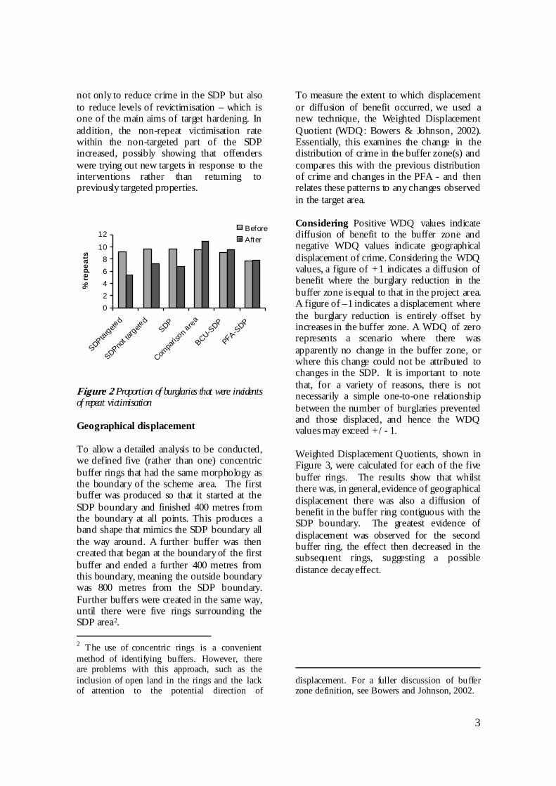
3

not only to reduce crime in the SDP but alsoto reduce levels of revictimisation – which isone of the main aims of target hardening. Inaddition, the non-repeat victimisation ratewithin the non-targeted part of the SDPincreased, possibly showing that offenderswere trying out new targets in response to theinterventions rather than returning topreviously targeted properties.

02468

10

12

SDPta rgeted

SDPnot ta

rgeted

SDP

Compa

rison a

rea

BCU-SDP

PFA-S

DP

% re

peat

s

BeforeAfter

Figure 2 Proportion of burglaries that were incidentsof repeat victimisation


To allow a detailed analysis to be conducted,we defined five (rather than one) concentricbuffer rings that had the same morphology asthe boundary of the scheme area. The firstbuffer was produced so that it started at theSDP boundary and finished 400 metres fromthe boundary at all points. This produces aband shape that mimics the SDP boundary allthe way around. A further buffer was thencreated that began at the boundary of the firstbuffer and ended a further 400 metres fromthis boundary, meaning the outside boundarywas 800 metres from the SDP boundary.Further buffers were created in the same way,until there were five rings surrounding theSDP area2. 2 The use of concentric rings is a convenientmethod of identifying buffers. However, thereare problems with this approach, such as theinclusion of open land in the rings and the lackof attention to the potential direction of

To measure the extent to which displacementor diffusion of benefit occurred, we used anew technique, the Weighted DisplacementQuotient (WDQ: Bowers & Johnson, 2002).Essentially, this examines the change in thedistribution of crime in the buffer zone(s) andcompares this with the previous distributionof crime and changes in the PFA - and thenrelates these patterns to any changes observedin the target area.

Considering Positive WDQ values indicatediffusion of benefit to the buffer zone andnegative WDQ values indicate geographicaldisplacement of crime. Considering the WDQvalues, a figure of +1 indicates a diffusion ofbenefit where the burglary reduction in thebuffer zone is equal to that in the project area.A figure of –1 indicates a displacement wherethe burglary reduction is entirely offset byincreases in the buffer zone. A WDQ of zerorepresents a scenario where there wasapparently no change in the buffer zone, orwhere this change could not be attributed tochanges in the SDP. It is important to notethat, for a variety of reasons, there is notnecessarily a simple one-to-one relationshipbetween the number of burglaries preventedand those displaced, and hence the WDQvalues may exceed +/- 1.

Weighted Displacement Quotients, shown inFigure 3, were calculated for each of the fivebuffer rings. The results show that whilstthere was, in general, evidence of geographicaldisplacement there was also a diffusion ofbenefit in the buffer ring contiguous with theSDP boundary. The greatest evidence ofdisplacement was observed for the secondbuffer ring, the effect then decreased in thesubsequent rings, suggesting a possibledistance decay effect.

displacement. For a fuller discussion of bufferzone definition, see Bowers and Johnson, 2002.

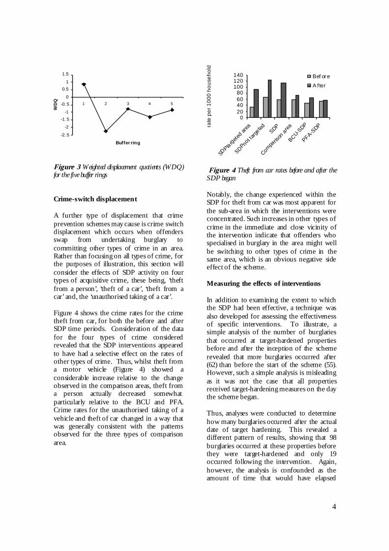
4

-2. 5

-2

-1. 5-1

-0. 50

0.51

1.5

1 2 3 4 5

Buffer ring

WD

Q

Figure 3 Weighted displacement quotients (WDQ)for the five buffer rings

Crime-switch displacement

A further type of displacement that crimeprevention schemes may cause is crime switchdisplacement which occurs when offendersswap from undertaking burglary tocommitting other types of crime in an area.Rather than focusing on all types of crime, forthe purposes of illustration, this section willconsider the effects of SDP activity on fourtypes of acquisitive crime, these being, ‘theftfrom a person’, ‘theft of a car’, ‘theft from acar’ and, the ‘unauthorised taking of a car’.

Figure 4 shows the crime rates for the crimetheft from car, for both the before and afterSDP time periods. Consideration of the datafor the four types of crime consideredrevealed that the SDP interventions appearedto have had a selective effect on the rates ofother types of crime. Thus, whilst theft froma motor vehicle (Figure 4) showed aconsiderable increase relative to the changeobserved in the comparison areas, theft froma person actually decreased somewhatparticularly relative to the BCU and PFA.Crime rates for the unauthorised taking of avehicle and theft of car changed in a way thatwas generally consistent with the patternsobserved for the three types of comparisonarea.

020406080

100120140

SDPtargete

d area

SDPnot ta

rgeted SDP

Compa

rison

area

BCU-SDP

PFA-SDPra

te p

er 1

000

hous

ehol

d

Bef or eA fter

Figure 4 Theft from car rates before and after theSDP began

Notably, the change experienced within theSDP for theft from car was most apparent forthe sub-area in which the interventions wereconcentrated. Such increases in other types ofcrime in the immediate and close vicinity ofthe intervention indicate that offenders whospecialised in burglary in the area might wellbe switching to other types of crime in thesame area, which is an obvious negative sideeffect of the scheme.

Measuring the effects of interventions

In addition to examining the extent to whichthe SDP had been effective, a technique wasalso developed for assessing the effectivenessof specific interventions. To illustrate, asimple analysis of the number of burglariesthat occurred at target-hardened propertiesbefore and after the inception of the schemerevealed that more burglaries occurred after(62) than before the start of the scheme (55).However, such a simple analysis is misleadingas it was not the case that all propertiesreceived target-hardening measures on the daythe scheme began.

Thus, analyses were conducted to determinehow many burglaries occurred after the actualdate of target hardening. This revealed adifferent pattern of results, showing that 98burglaries occurred at these properties beforethey were target-hardened and only 19occurred following the intervention. Again,however, the analysis is confounded as theamount of time that would have elapsed

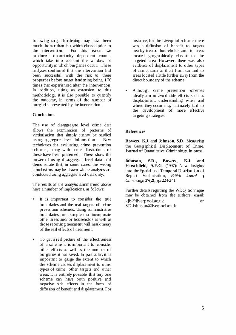
5

following target hardening may have beenmuch shorter than that which elapsed prior tothe intervention. For this reason, weproduced ‘opportunity dependent counts’which take into account the window ofopportunity in which burglaries occur. Theseanalyses confirmed that the intervention hadbeen successful, with the risk to theseproperties before target hardening being 1.76times that experienced after the intervention.In addition, using an extension to thismethodology, it is also possible to quantifythe outcome, in terms of the number ofburglaries prevented by the intervention.

Conclusions

The use of disaggregate level crime dataallows the examination of patterns ofvictimisation that simply cannot be studiedusing aggregate level information. Newtechniques for evaluating crime preventionschemes, along with some illustrations ofthese have been presented. These show thepower of using disaggregate level data, anddemonstrate that, in some cases, the wrongconclusions may be drawn where analyses areconducted using aggregate level data only.

The results of the analysis summarised abovehave a number of implications, as follows:

• It is important to consider the trueboundaries and the real targets of crimeprevention schemes. Using administrativeboundaries for example that incorporateother areas and/or households as well asthose receiving treatment will mask manyof the real effects of treatment.

• To get a real picture of the effectivenessof a scheme it is important to considerother effects as well as the number ofburglaries it has saved. In particular, it isimportant to gauge the extent to whichthe scheme causes displacement to othertypes of crime, other targets and otherareas. It is entirely possible that any onescheme can have both positive andnegative side effects in the form ofdiffusion of benefit and displacement. For

instance, for the Liverpool scheme therewas a diffusion of benefit to targetsnearby treated households and to areaslocated geographically closest to thetargeted area. However, there was alsoevidence of displacement to other typesof crime, such as theft from car and toareas located a little further away from thedirect boundary of the scheme.

• Although crime prevention schemesideally aim to avoid side effects such asdisplacement, understanding when andwhere they occur may ultimately lead tothe development of more effectivetargeting strategies.

References

Bowers, K.J. and Johnson, S.D. Measuringthe Geographical Displacement of Crime.Journal of Quantitative Criminology. In press.

Johnson, S.D., Bowers, K.J. andHirschfield, A.F.G. (1997): New Insightsinto the Spatial and Temporal Distribution ofRepeat Victimisation, British Journal ofCriminology, 37(2), pp. 224-241.

Further details regarding the WDQ techniquemay be obtained from the authors, email:[email protected] [email protected]

Pushing back the boundaries: new techniques for assessing ... · Pushing back the boundaries: new...

Documents

Transcript of Pushing back the boundaries: new techniques for assessing ... · Pushing back the boundaries: new...