Purchasing Power Parities for the Measurement of Global...

PPPs for the Measurement of Global and Regional Poverty:Issues and Options

D.S. Prasada RaoSchool of Economics

University of Queensland Brisbane, Australia

July 2003

This is a prepared for the Development Economics Data Group of the World Bank. The empirical analysis section is based on the work undertaken jointly by D.S. Prasada Rao and Chris O’Donnell of the School of Economics, University of Queensland. The authors wish to thank Ms. Jinsook Lee of DECDG of the World Bank for her efforts in securing unit record data from LSMS/HES, and Mr. Yonas Biru who has always been available for consultation on matters relating to this work.

1

I. General Background

The current practice of producing global poverty estimates makes use of $1/day and $2/day poverty lines. The use of these poverty lines is justified on the grounds that they closely correspond to the poverty lines used in some of the poorest countries, thus their application is likely to produce a conservative estimate of poverty incidence in the world. The approach also recognises the diversity of methodologies for setting poverty lines practiced in different countries. Using a single poverty line makes it possible to assess poverty incidence across countries and regions that is free from the influence of different country practices in setting poverty lines.

A crucial step in the process of compiling poverty estimates is the conversion of the $/day poverty line into respective national currency units. This conversion is made using PPPs from the International Comparison Program (ICP) for the Private Consumption Expenditure aggregate for the benchmark years. The Penn World Table PPPs for Consumption are also used for this purpose for the non-benchmark years. The national currency equivalent $/day poverty lines are used in conjunction with income distribution information to arrive at global and regional estimates of poverty incidence.

Over the last few years, the use of PPP data in the derivation of global and regional poverty estimates have attracted considerable attention and various limitations of the current approach have been identified. Deaton (2000) and Reddy and Pogge (2002) provide a comprehensive summary of some of the relevant issues.

Some of the principal issues are listed below.

The ICP-PPPs are based on prices of commodities that are not representative of the consumption baskets of the poor.

The ICP PPPs weight commodity-specific relative prices with weights that do not adequately represent the consumption patterns of the poor.

The aggregation methodology used does not offer a direct comparison of a fixed basket of goods and services consumed;

The PPPs used are not consistent, in their temporal movements, between benchmarks; The international poverty lines, $1/day or $2/day are not directly related to any

conception of poverty and therefore lack an analytical framework. The process of updating $1/day poverty lines over time is not clear.

It may be stressed here that the World Bank explicitly recognises some of these issues. Ravallion (2000 and 2002), in his replies to Deaton and Reddy and Pogge, defends the use of $1/day poverty lines and emphasises that “the vast bulk of Bank’s analytic and operational work on poverty, the ‘$/day” line is ignored, and with good reason. When one works on poverty in a given country, or region, one naturally tries to use a definition of poverty appropriate to that setting. Most of the time, the Bank’s poverty analysts don’t need to know what the local poverty line is worth in international currency at purchasing power parity…..” (Ravallion, 2002). The global and regional poverty estimates reported can be used only as a general guide to levels and broad trends in poverty, but cannot be considered as substitutes for the country-specific poverty estimates derived at national levels.

The current round of the International Comparison Program, scheduled for 2004, presents an excellent opportunity to examine the possibility of compiling poverty PPPs. Given the importance attached to global and regional poverty estimates within the context of the Millennium Development Goals (MDGs) with respect to poverty reduction, it is therefore necessary to integrate the work of poverty-PPP compilation with the regular ICP activities at the World Bank as well as at the national levels.

2

II. Poverty Specific PPPs: Basic Elements

An important starting point in the construction of poverty specific PPPs is to recognise that the tasks of setting international poverty lines and the construction of poverty-specific PPPs are two distinct components. The choice of the international poverty line is a task best undertaken by the Poverty Section of the World Bank’s Development Research Group, and should, therefore, be considered as being outside the domain of the current efforts to construct poverty-PPP. However, compiling poverty PPPs will involve a detailed examination of the methods and practices involved in setting poverty lines at the country level. Given the complex nature of the tasks involved, it is necessary to develop a close collaborative approach between the DECDG and the Development Research Group. Close consultation and a strong collaboration between those who coordinate the ICP and those who manage the World Bank poverty measurement and monitoring work are essential for successful completion of this work.

Several basic ingredients are necessary to construct PPPs for poverty measurement.

1. The first and foremost component is the price data. Since PPPs are essentially spatial price index numbers (for comparisons across countries), we need to collect data on prices “paid by the poor”. Several issues arise here. It is necessary to identify the poor in each country before price data are collected. This poses a problem of circularity in the tasks to be conducted. This issue can be resolved by using either country-specific rates of poverty incidence or rates of incidence implicit in previous World Bank publications. These could be considered as a reasonable starting point for the exercise. The second issue is to identify the goods and services that are typical of the consumption of the poor. The task of identifying “food” items may be easier than listing “non-food” items. In addition to identifying the list of items, it is also necessary to identify the type of outlets where poor make their purchases as well as the typical sizes of their purchase. It is also necessary to take into account possible regional and rural-urban variations in the list of consumption items.

2. The second element needed in PPP computation is data on expenditure shares that reflect the consumption patterns of the poor. It is expected that consumption pattern of the poor differs significantly from that of the average consumption pattern observed in a country. Again, there is need to identify the poor in order to be able to study their expenditure patterns.

3. The price and weights data from different countries need to be aggregated using a suitable index number methodology that can result in a set of PPPs.

The ultimate objective is to develop a framework to integrate the task of producing poverty-specific PPPs within the framework of ICP. The following are crucial steps in achieving this objective.

1. Examine the nature and extent of price data necessary for the construction of poverty-specific PPPs.

2. Identify the existing sources of price information within the institutional framework and price surveys conducted by the national statistical organisations.

3. Establish a survey framework for any additional price data required to supplement existing price data.

4. Propose a suitable aggregation methodology using the existing ICP practices and examine the sources of data on weights to be used in the aggregation process.

5. Investigate the problem of updating the international poverty line for temporal comparisons of global poverty estimates. The parallel problem of extrapolating poverty-PPPs for non-benchmark years will also be considered as a part of the ongoing poverty-PPP work.

3

III. A Pilot Study

A pilot study involving a total of eight countries, covering Cote d’Ivoire, Egypt, Ethiopia, Ghana, India, Indonesia, the Philippines and Thailand, with the following aims was conducted.

The starting point for the work was to examine: (i) country-specific practices in establishing poverty lines with the aim of identifying a basket of goods and services that may be truly termed a “poverty-basket”; (ii) if national statistical organisations regularly collect data on prices paid by the poorer sections of the population; (iii) the household expenditure survey data available in different countries to check if such data could be used in measuring prices paid by the poorer sections; and, finally, (iv) to extract expenditure shares, for commodity groups, that can be used as weights in aggregating price data.

A brief summary of the general findings is provided below.

There is a common thread in the methodology used in determining poverty lines in these countries. All poverty lines consist of food and non-food components, with the food component essentially being based on a specific energy requirement. Household expenditure surveys are the main source of data for this purpose. However, there are subtle differences in actual translation of caloric needs into monetary values. Non-food poverty line determination varies a great deal. None of these countries actually use or identify a consumption basket associated with the “poor”. Spatial and temporal adjustments of poverty lines are made using Laspeyres-type price index numbers.

All these countries rely on household expenditure (HES) or living standards measurement surveys (LSMS) as the principal source of data for poverty line determination and subsequent estimation of poverty incidence. Close examination of the survey questionnaires shows that these surveys collect fairly detailed information on total expenditure and quantity for various food and non-food items. The non-food items generally appear in a fairly aggregated form. These surveys often include non-market consumption (from own production and in-kind transactions) and an imputed value. These surveys provide useful unit value information that can be used to supplement price information collected from other sources.

The consumer price index compilation in these countries was closely examined. Special focus was placed on price indices for lower income groups and on spatial price comparisons within countries. There are a few countries where consumer price indices for low-income groups (eg the bottom 30% of the population and rural agricultural labourers) are regularly compiled and published. Another interesting observation emerging from discussions with officials at the national statistical offices is that very useful information on item and outlet specifications is collected as a part of CPI compilation, but which is not electronically compiled or disseminated.

IV. Price Level Comparisons using Household Expenditure Survey Data

As a part of this exploratory phase, econometric analysis of household expenditure survey data is being conducted. The aim is to derive unit values or average commodity prices and use them in measuring differences in price levels. The following are the principal aims of the empirical analysis.

1. Measuring price level differences across income groups. As a first step, average prices and quantities are derived for different income groups (eg decile groups) from the household expenditure surveys. Various binary and multilateral index number methods such as the

4

unweighted and weighted Elteto-Koves-Szulc (EKS) and the expenditure share weighted Geary-Khamis (GK) are being used in deriving consistent price index numbers.

2. Measuring price level differences across income groups using unit record data at the household level. In order to be able to make use of the very detailed data available from the household expenditure surveys, it is necessary to apply regression methods. The unweighted country-product-dummy (CPD) and weighted CPD methods are being used to handle household level data.

If price level differences across income groups can be measured unambiguously, it would be possible to adjust the current ICP-PPPs to derive more meaningful poverty-specific PPPs. Lack of quality information attached to consumption data in the household expenditure surveys is a major problem. If the higher income groups are shown to pay higher prices, this may be partly attributable to the higher quality of products included in their consumption.

3. Construction of PPPs for cross-country comparisons. Conceptually, it is possible to make use of the share weighted-GK, EKS or weighted CPD methods to combine data from the four countries to compute PPPs for price comparisons for different income groups. If the bottom three deciles (30%) are considered poor, PPPs associated with this bottom group may be considered more appropriate for poverty related work. Given the differences in product specification and detail in different household expenditure surveys, it may be necessary to apply this approach at a slightly more aggregated level.

4. Spatial Price Comparisons. Given unit record data, with details on the location of households by regions within each country, an attempt is being made to construct spatial/regional price index numbers for different income groups.

The pilot project, within its broad objectives, also examines the sensitivity of the derived PPPs to the aggregation methods used. The project considers a number of new aggregation methods such as the weighted EKS, share-weighted GK and weighted CPD, along with some of the standard methods. A brief description of these aggregation methods is provided in the following section.

IV.a. Aggregation Methods used in the study

The study made use of several binary index number formulae, such as the Paasche, Laspeyres, Fisher and Tornqvist, in deriving price index numbers for computing PPPs for income groups. In addition a number of multilateral index number methods including the Elteto-Koves-Szulc (EKS) and weighted EKS; the country-product-dummy (CPD) methods and number of variants of the methods; and the expenditure-share weighted Geary-Khamis method have also been employed. These aggregation methods are briefly described below.

IV.a.1. Binary Methods

Let pij and qij denote the price and quantity of product i in income group j. The following are the four commonly used binary index number formulae.

Paasche: Pjk =

Laspeyres: Ljk =

Fisher: Fjk =

Tornqvist: Tjk = exp[0.5(vij + vik)log(pij/pik)]

5

where vij = are value shares.

IV.a.2. Multilateral Methods

The current analysis of household expenditure survey data within the pilot project employs a range of new or modified aggregation methods. This section describes these methods and their properties. Further details of these methods can be found in the papers cited.

Method 1: Weighted EKS Method

The computational form for the Elteto-Koves-Szulc (EKS) index is given by

(1)

where Fjk denotes the Fisher price index number for country k with country j as the base. A simple interpretation of the EKS index is that any binary comparison between countries j and k is an unweighted averaged of all the linked comparisons between j and k using links l = 1, 2, …, M. Rao (2001) showed that the standard EKS is essentially based on the least squares estimation of the parameters of the simple regression equation:

(2)and

where ’s are the ordinary least squares estimators of ’s.

Using this approach, weighted EKS comparisons can be obtained by simply altering the distribution of the random disturbance term in model (2) as where wjk is a measure of reliability attached to a given binary comparison. These weights can be used in accounting for a variety of data and measurement related problems. Rao et al. (2002) and Rao and Timmer (2003) provide useful applications of the weighted EKS to comparisons of agricultural and manufacturing sector output and productivity. Selection of weights within the EKS method may vary according to the level (below or above basic heading level) at which the method is applied. Rao (2001) provides a few illustrative examples of the type of weights that can be used in improving the EKS comparisons.

Method 2: Expenditure Share Weighted Geary-Khamis Method

The Geary-Khamis (GK) method, which was used in most international comparisons until recently, is often criticised due to the Gerchenkron effect in real income comparisons resulting from its use. The main driver of this effect is the definition of international prices used in the method. The GK method consists of the following interrelated equations:

and (3)

where Pi’s are international prices.

6

It is clear from (3) that the international price of a commodity is defined as a weighted average of national prices, with weights proportional to the quantities. Therefore, there is a tendency within the GK method to be influenced by prices observed in richer and larger countries. However, one of the advantages of the GK method is that it satisfies additive consistency which allows for sectoral share analysis.

The expenditure-share weighted GK method is a modified version of the GK method designed to make it size neutral and yet provide an additively consistent set of comparisons. The method uses the following definition of international prices:

where is the value share (4)

The use of equation (4) can be justified on the basis that these international prices track observed prices and minimise the following sum of squares of deviations:

Rao (2000) shows that the expenditure-share weighted GK method is feasible in that it has a solution which is positive and unique up to a factor of proportionality.

The usefulness of this method lies in the fact that it preserves additive consistency (like the GK method) and at the same time makes it size neutral (like the EKS method).

Method 3: Weighted Country-Product-Dummy (CPD) Method

The standard CPD formulation, due to Summers (1973), is a simple regression model that regresses logarithm of observed prices on a set of dummy variables representing the commodity and country to which a given price observation refers to. It uses the following regression model

(5)with D’s and D*’s, respectively, refer to country and product dummy variables. This formulation was used in handling missing observations and it was also used as a method for aggregating price data below the basic heading level.

Rao (1995) established that it is feasible to consider a generalisation of the CPD method which can be used for aggregation above the basic heading level. Rao proposed an extension that allows for the use of weights – an extension with its roots in weighted least squares – with weights reflected by the expenditure shares. The model in Rao (1995) is equivalent to running the following regression model with transformed observations.

(6)The required PPP’s are simply given by where is the least-squares estimator of in equation (6).

Even though the weighted CPD is a simple extension of the CPD model, Rao (2001) has demonstrated that it is a powerful technique with very important properties. A few of these are listed below.

7

The weighted CPD method is equivalent to the Rao (1990)-system for multilateral comparisons. This result, proved in Rao (1995), establishes a link between the econometric approach and the standard PPP and International Price approach in the Geary-Khamis method. Since the weights here are based on shares, this method is size-neutral.

When applied to binary comparisons, the method results in index numbers that are superlative. In fact it is possible to obtain an explicit form in the case of binary comparisons and the resulting index is a geometric average of price relatives (similar to the Tornqvist index). Diewert (2002) shows that a number of other indices can also be generated by varying the CPD model specification.

The weighted CPD model allows for a more complex specification of the disturbances. For example, spatial structures in price relatives can be gainfully exploited and incorporated into the computations through a spatially autocorrelated disturbance specification (see Rao, 2001 for more details).

The CPD model can be viewed as a simplified hedonic model. This interpretation suggests the possible use of the generalised CPD method to include quality characteristics explicitly in the regression specification. Incorporation of quality and outlet characteristics allows for the use of a more general approach to international comparisons where the standard approach of pricing very tightly specified items can be replaced by an approach based on loosely specified items with all the specifications recorded for each price observation. As a result of this approach it is possible to improve respresentativeness of the baskets priced for purposes of the ICP.

The CPD method is particularly useful in handling unit record data from household expenditure surveys to construct PPPs for regional price comparisons. Aten and Menezies (2002) and Coondoo et al. (2002) used the weighted CPD method, proposed in Rao (2001), to study regional price differences in Brazil and India. Neither the weighted EKS nor the expenditure share weighted GK can handle detailed unit record data. The weighted CPD is currently being used in the analysis of unit record data from Ethiopia, Ghana, Indonesia and the Philippines to estimate PPPs.

IV.b. Empirical Results

Analysis of Ethiopian Household Expenditure Survey Data

Results from the analysis of Ethiopian household expenditure survey data for the year 2000 are presented in the following section. Agents from the Ethiopian Central Statistical Authority visited each household every week for four weeks, and collected the quantity and value of food and drinks consumed at home (including own production and goods obtained free).

The Ethiopian data set is a large data set with data consisting of 607,314 observations. Percentage distribution of these households by regions is shown in the table below.

Table 1: Regional Distribution of the Samplein the Household Expenditure Survey

Region % of observationsTigray 6.24Afar 3.32Amhara 16.59Oromiya 23.59Somalie 4.39BenshangulGumuz 5.92

8

SNNP 16.04Gambela 4.11Harari 5.08Addis Abbaba 9.43Dire Dawa 5.28

Expenditures are measured in Birr (1.00 Australian Dollar = 5.2 Ethiopian Birr). Quantities are measured by the gram (eg. most grains), cubic centimetre (eg. most beverages), or number of items (eg. cigarettes). These units of measurement are small, which may explain why some reported quantities appear large (and therefore unit prices appear small).

The household expenditure data are provided in detail for a total of 262 products of which 252 refer to items of food expenditure. Tabulation of data for non-food expenditure is considered insufficient for any meaningful measurement of price level differences in non-food items across income groups. So the empirical analysis reported below is essentially limited to data on prices and expenditures of food items.

A product listing is provided in Appendix Table A. 1, together with average expenditures and average quantities consumed. The average expenditures (quantities) reported in this table were computed as the coefficients from a regression of item expenditure (quantity) on 252 product dummy variables.

Implicit prices were calculated by dividing item expenditures by item quantities. Average (implicit) prices and quantities were calculated for each of 10 income groups by selecting the observations in each group and using them to regress prices (or quantities) on the 252 product dummy variables.

V.b.1. Binary Price Index Numbers by Income Groups

Average prices and quantities by income group were used to construct Paasche, Laspeyres, Fisher and Tornqvist indices. Appendix Table A.2 presents matrices of order 10 x 10 calculated using each of these formulae. As these indices are not transitive, relative price level differences vary depending upon which income group is used as the base group for purposes of index calculation. For purposes of interpreting results, the first column of Appendix Table 2 shows price index numbers for various income groups calculated using the first decile (poorest 10%) as the base group. Price indices for the 3rd group, using the 1st group as the base (=1.00), calculated using Paasche, Laspeyres, Fisher and Tornqvist indices are respectively given by 1.109; 0.928; 1.014 and 1.019. A large gap in the Laspeyres and Paasche indices is to be noted here. This is an indication that price indices could be sensitive to the formula used.

The authors have investigated possible reasons for a sizeable divergence between Fisher and Tornqvist indices. These indices, considered as “superlative indices”, usually have numerical values of similar magnitude.

Results from the application of binary index number methods are reported under Models A, B, C and D.

V.b.2. Multilateral Index Numbers by Income Groups

A battery of multilateral index number formulae have been employed in measuring price level differences across income groups. The principal methods are the weighted EKS, weighted CPD and the expenditure-share weighted Geary-Khamis Method.

9

The EKS and Weighted EKS methods used in the study

The weighted EKS methods crucially depend upon the weights used. We consider three different weighting matrices leading to a total of four (one unweighted and three weighted) sets of EKS indices. In addition to the standard EKS indices derived using the Fisher binary formula, we have also used binary-Tornqvist indices in the construction of EKS indices. This approach resulted in the following Models.

E: Unweighted EKS using Fjk

F: Weighted EKS using Fjk and P-L spreadG: Weighted EKS using Fjk and |i-j|H: Weighted EKS using Fjk and 1/jk

I: Unweighted EKS using Tjk

J: Weighted EKS using Tjk and P-L spread

Where

the Paasche-Laspeyres spread, calculated as PLSjk = |ln(Ljk/Pjk)| the ‘distance’ between income groups i and j, crudely measured as |i – j|. 1/ij, where ij denotes the correlation between the quantities consumed by groups i

and j.

The matrices of Paasche-Laspeyres spreads and quantity correlations are presented in Table A.3 of the Appendix.

All the indices based on the EKS method and its variants (Models E to J) are calculated using the average prices and average quantities for all the food items. These are averages of household expenditures and quantities of all the households belonging to the specific income groups.

The CPD and weighted CPD variants used in the study

The country-product-dummy method is a regression-based method which is ideal to deal with large data sets in the form of household-specific price, quantity and expenditure information. The CPD index numbers presented in various tables are essentially exponentials of estimated coefficients associated with the dummy variable representing various income groups. In all the calculations, we use the first income-group as the base. Several variants of the CPD have been used in the current study.Models K and N: These are the unweighted and weighted CPD models described in Section IVb. The weights used here are expenditure shares that show the importance of a particular item of consumption within the food basket. Estimated regression coefficients for various models are presented in Table A.4 in the Appendix.

Models L and O: These models use income as an additional explanatory variable in the regression model. Inclusion of the variable is based on some recent work of Coondoo et al. (2002) where the income variable is considered as a proxy for variation in the quality of items consumed. It is generally considered that higher income group households consumer better quality products. Inclusion of this variable is expected to make an automatic adjustment of quality of products. We note here that estimated coefficients, in Appendix Table A.4, show little impact of the inclusion of income as an explanatory variable.

Models M and P: The CPD model is versatile enough to provide estimates of regional price level differences along with income-group price differentials. These models are estimated after including regional dummy variables.

10

Models K to P have been estimated using GAUSS programme and these models make use of the complete household-specific price and expenditure data.

Models Q and R: As the binary index numbers and the EKS index numbers are only based on only income-group averages on expenditure and prices, the CPD and weighted CPD models L and O have been replicated using only average data. Estimates of coefficients for these models have been derived using SHAZAM programme.

Model S: This model refers to the expenditure-share weighted Geary-Khamis method. These results are obtained by solving a system of non-liner equations. It uses 10 income groups and as in the case of Fisher and EKS and it can only make use of average price and expenditure data for each income group.

Estimated coefficients from the use of CPD regressions on unit record data and income group averages are presented in Tables A.4 and A.5 of the Appendix.

In addition to these, we have also applied all these aggregation methods to more aggregated data consisting of only three income groups: Low Income (bottom 30%); Middle Income (middle 60%); and High Income (Top 10%).

V.c. Estimates of Price Level Differences across income groups

We first present results calculated using various binary index number formulae, a number of variants of the EKS and the CPD models, and also using the expenditure-share weighed G-K method. These are presented in Table 2. The following are a few salient features.

All the results presented are expressed relative to the first decile or the lowest income group for which the price index is 1.00.

A general finding from these results is that the top two income groups pay higher prices relative to the bottom decile group. However, some of the intermediate income groups appear to pay lower prices than those in the bottom group.

Generally there is a significant gap between the Laspeyres and Paasche indices. This indicates a divergence in price and quantity structures across income groups. We also suspect that a part of this gap is also due to the presence of a number of items which have zero expenditure.

11

TABLE 2 Binary, EKS and CPD Index Numbers - 10 Income Groups A: Paasche (Base = Group 1) 1.000 1.757 1.109 1.048 1.011 1.017 1.013 1.178 1.055 1.262 B: Laspeyres (Base = Group 1) 1.000 0.999 0.928 0.948 0.978 0.986 0.967 0.997 1.007 1.041 C: Fisher (Base = Group 1) 1.000 1.325 1.014 0.997 0.994 1.001 0.990 1.084 1.031 1.146 D: Tornqvist (Base = Group 1) 1.000 1.000 1.019 0.981 1.001 0.981 1.009 0.996 1.007 1.022 E: Unweighted EKS using Fjk 1.000 1.254 1.044 0.999 1.032 1.017 1.007 1.055 1.052 1.101 F: Weighted EKS using Fjk and P-L spread 1.000 1.281 1.113 1.018 1.055 1.046 1.014 1.077 1.078 1.117 G: Weighted EKS using Fjk and |i-j| 1.000 1.262 1.035 1.007 1.032 1.019 1.006 1.054 1.051 1.106 H: Weighted EKS using Fjk and 1/jk 1.000 1.253 1.042 0.998 1.030 1.016 1.005 1.054 1.051 1.100 I: Unweighted EKS using Tjk 1.000 0.992 0.984 0.987 1.009 0.987 1.005 1.004 1.016 1.034 J: Weighted EKS using Tjk and P-L spread 1.000 0.996 0.994 0.992 1.011 0.994 1.007 1.008 1.021 1.034 K: CPD 1.000 0.997 0.997 0.996 0.997 1.001 1.010 1.005 1.007 1.018 L: CPD with Income 1.000 0.997 0.997 0.996 0.997 1.000 1.009 1.004 1.006 1.016 M: CPD with Regional Dummies 1.000 0.998 0.998 0.996 0.997 0.999 1.002 1.002 1.006 1.017 N: Weighted CPD 1.000 0.998 0.998 1.002 1.005 1.014 1.025 1.021 1.020 1.028 O: Weighted CPD with Income 1.000 0.998 0.998 1.001 1.004 1.013 1.023 1.019 1.017 1.021 P: Weighted CPD with Regional Dummies 1.000 0.997 0.997 1.000 1.001 1.007 1.011 1.012 1.012 1.018 Q: CPD using average data 1.000 0.983 0.985 0.990 1.007 0.981 0.993 1.015 1.015 1.061 R: Weighted CPD using average data 1.000 0.991 0.971 0.989 1.008 0.987 1.010 0.997 1.019 1.039 S: Exp.-share weighted Geary-Khamis 1.000 1.002 0.955 0.988 1.006 0.985 1.008 0.993 1.011 1.036

12

All the indices based on the CPD method and its variants show that prices paid by the lowest income group are higher than those paid by the second, third and fourth decile groups. This shows that the very poor may be paying more than their immediate decile group households.

Generally the top three decile group households face higher prices than those in the bottom decile groups.

Indices based on Fisher and the EKS indices computed using Fisher binaries show that bottom three decile groups generally pay higher prices than the richer households. We believe that this is mainly due to the treatment of items which had zero expenditures recorded.

Results in Table A.6 suggest that once all the products with zero expenditures for at least one of the expenditure groups are removed, then the bottom groups show lower price levels than the top decile groups.

Index numbers based on Tornqvist binary index numbers appear to be very close to those generated by the weighted CPD method. This is consistent with the properties of weighted CPD method outlined in Rao (2001).

Since income groups in the multilateral comparisons here have a natural order, poorest decile to the top decile, we have also computed chain index numbers linking binary index numbers in an ascending order. These chained indices are presented in Appendix Table A.7. It is evident from this table that there is considerable spread between the Laspeyres and Paasche indices. However, the chained Tornqvist indices appear to be quite close to both weighted CPD and Tornqvist based EKS indices.

Figures 1 to 4 in the Appendix show price level differences across income groups based on various index number formulae. Results in Figure 3 are of particular interest. These results show that CPD method yields results that are fairly consistent in their trends.

The main conclusion that can be drawn from the results presented in this section is that the weighted CPD and the Tornqvist based indices provide fairly similar estimates of price level differences between income groups. These results appear to be fairly robust to minor variations in terms of model specification and the use of different sets of weights. The results also show sensitivity of Laspeyres, Paasche and Fisher indices to the presence of zero-expenditure observations in the data. Dropping all those items which have a zero expenditure recorded for at least one of the income groups appear to provide more meaningful Laspeyres, Paasche and Fisher indices. However, a significant loss of information may occur if this were to be followed as a standard procedure. In contrast, the CPD method and its variants make use of all available data.

Analysis of Ugandan Household Expenditure Survey data

We present some interim results from the analysis of the household expenditure survey data from Uganda for the year 1999/2000. Analysis of this data set is in progress.

Data was obtained from the Socioeconomic Survey conducted by the Uganda Bureau of Statistics (UBS) as part of its Uganda National Household Survey (UHNS) 1999/2000. Section 7 of the survey collects information on values and quantities purchased of 53 items in the food, beverages and tobacco group – Table A.8 lists these items and associated average expenditures and quantities. Table A.9 lists the non-durable and semi-durable items included in the Socioeconomic Survey – these items have not been included in this analysis.

The Socioeconomic Survey reports quantities and values for items in four categories – purchases for the household, purchases away from the household, consumption out of home produce, and free gifts. Consumption out of home produce and free gifts appear to be valued at market prices. In this analysis we do not discrimminate between these different types of

purchases – we obtain total quantities and values by summing quantities and values across the four categories, and then obtain implicit prices by dividing total values by total quantities.

Average (implicit) prices and quantities were calculated for each of 10 income groups by selecting the observations in each group and using them to regress prices (or quantities) on the 53 product dummy variables.

Table A.10 presents binary Laspeyres, Paasche, Fisher and Tornqvist indices for the ten decile groups. Indices from the Tornqvist and Fisher indices are generally close as one would expect from these two superlative index numbers.

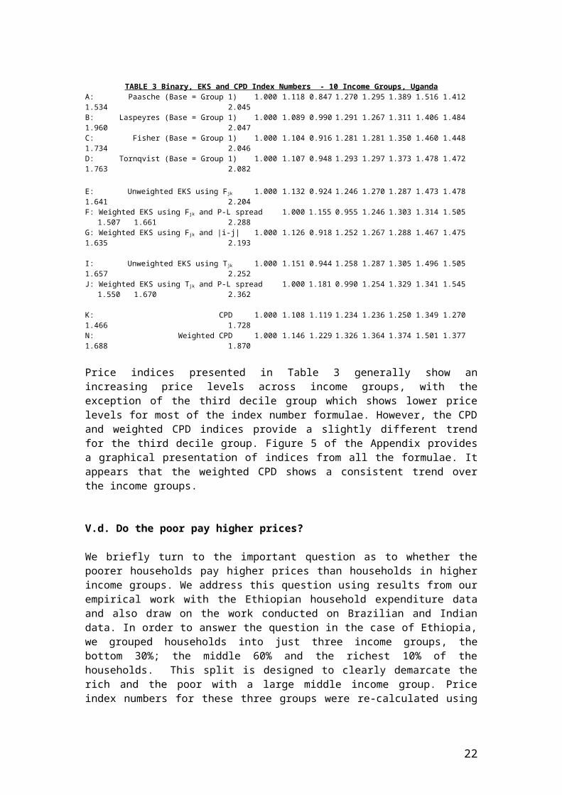
Table 3 presents various measures of price level differences calculated using a range of binary and multilateral methods. These methods are listed in the previous section.

TABLE 3 Binary, EKS and CPD Index Numbers - 10 Income Groups, UgandaA: Paasche (Base = Group 1) 1.000 1.118 0.847 1.270 1.295 1.389 1.516 1.412 1.534 2.045B: Laspeyres (Base = Group 1) 1.000 1.089 0.990 1.291 1.267 1.311 1.406 1.484 1.960 2.047C: Fisher (Base = Group 1) 1.000 1.104 0.916 1.281 1.281 1.350 1.460 1.448 1.734 2.046D: Tornqvist (Base = Group 1) 1.000 1.107 0.948 1.293 1.297 1.373 1.478 1.472 1.763 2.082

E: Unweighted EKS using Fjk 1.000 1.132 0.924 1.246 1.270 1.287 1.473 1.478 1.641 2.204F: Weighted EKS using Fjk and P-L spread 1.000 1.155 0.955 1.246 1.303 1.314 1.505 1.507 1.661 2.288G: Weighted EKS using Fjk and |i-j| 1.000 1.126 0.918 1.252 1.267 1.288 1.467 1.475 1.635 2.193

I: Unweighted EKS using Tjk 1.000 1.151 0.944 1.258 1.287 1.305 1.496 1.505 1.657 2.252J: Weighted EKS using Tjk and P-L spread 1.000 1.181 0.990 1.254 1.329 1.341 1.545 1.550 1.670 2.362

K: CPD 1.000 1.108 1.119 1.234 1.236 1.250 1.349 1.270 1.466 1.728N: Weighted CPD 1.000 1.146 1.229 1.326 1.364 1.374 1.501 1.377 1.688 1.870

Price indices presented in Table 3 generally show an increasing price levels across income groups, with the exception of the third decile group which shows lower price levels for most of the index number formulae. However, the CPD and weighted CPD indices provide a slightly different trend for the third decile group. Figure 5 of the Appendix provides a graphical presentation of indices from all the formulae. It appears that the weighted CPD shows a consistent trend over the income groups.

V.d. Do the poor pay higher prices?

We briefly turn to the important question as to whether the poorer households pay higher prices than households in higher income groups. We address this question using results from our empirical work with the Ethiopian household expenditure data and also draw on the work conducted on Brazilian and Indian data. In order to answer the question in the case of Ethiopia, we grouped households into just three income groups, the bottom 30%; the middle 60% and the richest 10% of the households. This split is designed to clearly demarcate the rich and the poor with a large middle income group. Price index numbers for these three groups were re-calculated using all the main formulae. Price indices for these three groups are presented in Table 3 below.

TABLE 3 Binary, EKS and CPD Index Numbers - 3 Income Groups

14

Ethiopia

Bottom 30% Middle 60% Top 10%A: Paasche (Base = Group 1) 1.000 1.024 1.058B: Laspeyres (Base = Group 1) 1.000 0.737 0.729C: Fisher (Base = Group 1) 1.000 0.869 0.878D: Tornqvist (Base = Group 1) 1.000 1.015 1.054

F: Weighted EKS using Fjk and P-L spread 1.000 0.868 0.879J: Weighted EKS using Tjk and P-L spread 1.000 1.015 1.054

N: Weighted CPD 1.000 1.015 1.029

Uganda

K: CPD 1.000 1.207 1.604N: Weighted CPD 1.000 1.279 1.672

It is clear from Table 4 that answer to this question cannot be unambiguously answered. Results are sensitive to the index number formula used in the computations. In the case of Ethipia, the Paasche, Tornqvist, weighted EKS with Tornqvist, and the weighted CPD generally show that the top decile group households face higher price levels than those in the bottom 30%. The exact magnitude varies between 2.9% (weighted CPD) to 5.8% (Paasche binary index). In contrast, the use of Laspeyres, Fisher and Fisher-based EKS indices show that richer households face much lower prices. It varies between 12.2% to 27.1%.

Based on the susceptibility of Laspeyres, Paasche and Fisher indices to the presence of zero-expenditures in some of the decile groups, we believe that it is more likely that the poorer households face slightly lower prices and this difference could even be lower if it were possible to make adjustments for differences in quality of the consumption items.

In the case of Uganda, the price increases over the income groups are more pronounced than in the case of Ethiopia. It is likely that even after adjustments for quality differences in items consumed by the higher and lower income groups the general trends in price levels show an increasing trend.

Now we turn to evidence from some other comparable studies. We draw on two studies, one on Brazil and another on India. While the Brazilian study mainly focused on the question of price level differences between income groups, the Indian study’s main objective was to examine regional differences in prices. Both of these studies make use of the weighted CPD and have not conducted any exhaustive examination of the robustness of their results to the choice of index number methodology.

Brazilian Study

Aten and Menezies (2002) analysed data from a Brazilian national survey known as POF (Pesquisa de Orcamento Familiar) for the year 1995-96 with a sampling frame of 12.5 families in eleven metropolitan cities. Actual data analysed consists of data recorded for 16,000 households for 41 food products. The weighted CPD model was used in their analysis. Aten and Menezies report results on 30 income classes as well as at a more aggregated level for three income groups. Results reported in Table 8 of Aten and Menzies shows the following price level differences for three income groups.

Price Indexes byIncome Groups

15

Low 1.000Middle 1.025High 1.091

Source: Aten and Menezies (2002)

Their results suggest that the higher income households in the top income groups pay, on average, 9.1% more than what the poorest one-third of households in Brazil pay. As we suggested in the introductory sections, if adjustments for quality were made then the price level for higher income groups could be lower. Therefore, the answer to the question as to whether poor pay higher prices can be answered in the negative with a caveat concerning quality adjustments.

Indian Study

Coondoo, Majumdar and Ray (2003) attempt to estimate regional consumer price differentials using the National Sample Survey data from the 50th round for the year 1993-94. Their method of estimation is essentially an application of the country-product-dummy method used in our own analysis. Though their main objective was to assess regional price differentials, they also estimated differences in prices paid by poor and non-poor households in rural and urban India. The following results are reported in their Table 3 which is reproduced below:

Household Group Rural India Urban India

South East West South East West

All Households

Households above poverty line

Households below poverty line

0.990

0.974

1.082

1.095

1.084

1.101

0.996

0.998

1.092

0.931

0.925

1.058

1.041

1.043

0.994

0.961

0.952

1.009Source: Coondoo et al. (2003)

Results in this table show interesting patterns. In Rural and Urban South and Western India, poorer households generally pay higher prices than households above poverty line. However in the case of Eastern regions these results show a slightly different trend. There may be some evidence in their study that poorer households may be paying more than richer households. This interpretation has to be made with a caveat. All the indices shown here are relative to the Northern region of India and the indices are relative to the group in Northern India. So Rural households in South India pay 8.2% higher prices than poorer households in North India whereas the richer households in South India pay 2.6% less than the richer households in North India. As their study does not provide estimates of price level differences within North India across income groups, it is a bit difficult to derive definite conclusions on the prices paid by the poor.

V.e. Conclusions from the empirical work

In summary, these three studies covering countries from three different continents show that generally poorer households do not necessarily pay higher prices. These studies also demonstrate that it is feasible to use household expenditure data to estimate price level differences across income groups. What are the implications for the computation of PPPs for global and regional poverty measurement? The following conclusions can be drawn from the current study.

16

Income group price differences

It is possible to derive adjustment factors for the PPPs derived from the ICP with the assumption that the ICP PPPs refer to the consumption of the high income households.

Estimates of price level differences do not show that prices paid by poorer households are higher than those paid by the richer households. It is possible that once adjustments for quality differences are made it may turn out that poorer households may be paying more for goods and services than richer households.

Results derived appear to be sensitive to the aggregation methodology used. The CPD method and its variants appear to provide more consistent results when compared to the index numbers derived using Laspeyres, Paasche, Fisher and Fisher-based EKS index numbers. The empirical analysis reported in this paper showed that presence of zero-expenditures can have an influence on the indices computed. Careful attention needs to be paid to this problem

Results do not appear to be sensitive to the use of aggregated data by income groups. Use of household level data offers rich alternatives. However, if the motive is one of making price comparisons across income groups, it is enough to focus on grouped data and average price and expenditures for income groups.

Role and use of household expenditure surveys in Poverty PPP work

The current study reported on an extensive empirical analysis of Ethiopian household expenditure survey data. It summarised results from studies conducted in Brazil and India. The following general observations can be made.

If household expenditure surveys are to be used as the principal source of price data, then it is necessary to synchronise the conduct of such surveys. These surveys are usually conducted once in every three or five years. Differences in survey years can pose a problem of comparability. For example, we could not make use of Susenas 2000 data from Indonesia since it did not include the consumption module.

Household expenditure surveys are a good source of prices and expenditures for food consumption. It is indeed difficult to get any meaningful price data on non-food consumption out of the household expenditure surveys. Therefore it is necessary to develop appropriate survey instruments to collect non-food price data.

As it is generally acknowledged, household expenditure surveys are the principal source of expenditure patterns and weights. These weights can be derived for income groups, regions or any other grouping of households. As expenditure shares are stable of over time, non-overlapping household survey dates do not pose a problem.

Household expenditure surveys and implicit price data in the form of unit value ratios appear to be a very useful source to measure price level differences across income groups and regions. As a first level of approximation, it should be possible to use these measures for purposes of adjusting ICP PPPs that are based on specially collected price data.

VI What are the options?

There are several feasible options with respect to the estimation of PPPs for global and regional poverty measurement. The status quo of using ICP PPPs for the Private Consumption Expenditure Aggregate is not a desirable option. The ICP PPPs are based on prices of goods and services that may have little overlap with the items generally consumed by the poor. The weights used in aggregating price data in the process of deriving PPPs are the national averages and, therefore, may not accurately reflect the consumption patterns of the poor. On the basis of the discussion and results presented in this paper, the following options may be canvassed for the derivation of PPPs for poverty measurement.

17

Option 1. Reweight the basic heading parities using expenditure patterns of the poor

A step towards addressing some of the recent criticisms is to use the expenditure patterns of the poor in aggregating price data collected as a part of the ICP exercise. This means that no special price surveys are conducted and item lists are prepared as per the new ICP Manual. These lists will have a regional character as the next round of ICP is going to be conducted on a regional basis. Prices used in the PPP computations are collected using tightly specified product specifications and annual national average prices are collected and used in regional comparisons. A set of ring countries will be used in constructing global comparisons from regional comparisons.

It would be necessary to compile expenditure patterns of the poor from each country. In order to identify the poor, one may use either national or international sources. The latest rounds of household expenditure/living standards measurement surveys may be used as a source of the expenditure patterns. If current HE/LSMS survey data are not available for some participating countries, it may be necessary to construct some weights based on old surveys or from surveys from neighbouring countries.

The main disadvantage with this approach is that the price data underlying PPP calculations would not refer to the prices paid by the poor. The ICP item lists, especially those constructed using tight product specifications with specific quality and brand characteristics, have more in common with the purchased made by upper middle and higher income groups. This is particularly the case with developing countries. It is also possible that the size of the items (eg 1kg packages of suigar) are not typical of the purchase behaviour of the poor who are constrained to buy much smaller quantities. Unit prices are usually much higher when purchased in small quantities.

Given these observations, reweighting the standard ICP price data and PPPs at the basic heading level in deriving PPPs for poverty measurement will still leave considerable scope for criticism.

Option 2. Employ adjustment factors to modify ICP PPPs

Recognising the fact that the ICP PPPs provide a measure of price level differences that are based on items that are representative of the purchase behaviour of the upper income group and that the prices used in ICP calculations are more closely related to the prices paid by these groups, an option for consideration is the use of some adjustment factors which can be used in deriving PPPs for the lower income groups.

These adjustment factors, to be meaningful, need to reflect differences in levels of prices paid by households in different income groups. Some of the empirical research reported in this paper and by others show that there are significant differences in price levels for income groups. Most of the studies show that richer households tend to pay higher prices compared to low income households. These results do not support the premise that poorer households generally pay higher prices.

Several qualifications need to be made. The first and foremost is that all the above mentioned studies are based on household expenditure data and the implicit prices derived in the form of unit values. Since unit values are essentially average prices for broadly defined commodities, the price differences observed are severely influenced by quality differences. If higher income households consumer better quality products and lower income groups purchase lower quality products, then adjusting for quality differences could alter the general conclusions. However, quality information is lacking in household expenditure surveys. The second problem that arises in the use of household expenditure survey data is that in many countries unit values can be derived only for food items. In many surveys, very detailed data are compiled for food

18

items – including information on consumption from own production and frequency as well as data on expenditure and quantities consumed/purchased. However, when it comes to non-food items only total expenditure under each item is recorded. Countries like Uganda and India, where expenditure and quantity data are available for non-food items, are more of an exception.

Based on the empirical analysis of household expenditure data, this option has limited viability in that adjustment factors can be derived only for food component of the consumption basket.

Option 3. Use ICP Price Data collected using Structured Product Descriptio n(SPD) approach with Loose Specifications

The Structure Production Description (SPD) approach is an approach that is under serious consideration for use in the next round of ICP. It marks a departure from the standard ICP practice of creating item lists where each item is tightly specified and then priced in different countries. The SPD approach uses loosely specified item lists and when ever an item is priced the item characteristics are also compiled. The SPD approach allows for the use of a product list that is representative of the items consumed in participating countries and at the same time achieves comparability through the use of data on item characteristics. Item characteristics may refer to a list of quality characteristics or they may refer to a geographical location where the product is priced (eg rural or urban areas) and the type of outlets where the item is priced (eg small retail outlets, general/open markets, supermarkets, a/c supermarkets, etc). The SPD approach also allows for the collection of data on the size of purchases. The SPD approach makes it possible to use price data collected for purposes of CPI construction within the ICP.

Under the SPD approach it is possible to identify those price quotations that are collected from markets or outlets that are typically used by poorer sections of the society. It is possible that higher income households may also make use of these outlets. It is feasible to explicitly account for the typical size of purchases made by the poor and use price quotations under the SPD approach that refer to similar size purchases.

Once price data are collected for ICP using the SPD approach, then it is possible to identify those price quotations that are relevant for purposes of computing PPPs for poverty measurement. These price quotations can then be combined with expenditure share data specific to poor in deriving PPPs.

An implication of the use of the SPD approach is that it would be necessary to abandon the use of national average prices as the basic price data collected for purposes of the ICP exercise. The volume of price data to be processed, under the SPD approach, is likely to be quite large. Therefore it would be necessary to use a more streamlined and computerised approach to price data collection in the next round of ICP.

Option 4: Collect Poverty-PPP specific price data

An option that addresses all the concerns of the users of poverty statistics would be to construct PPPs that are based on price data collected specifically for the purpose of poverty PPPs. The underlying task would be somewhat similar to that currently used for the general ICP, but on a much smaller scale. The general ICP covers goods and services that enter all the expenditure-side aggregates in gross domestic product. These include private consumption, government, capital formation and net exports. In contrast, poverty PPP work requires collection of data on prices of items that enter the consumption of the poor thus the scope is somewhat limited in comparison with the ICP.

19

The task of identifying items that enter the consumption of the poor may be simpler than the task of compiling a list for ICP – however, it would be necessary to involve regional poverty experts in drawing up such a list. It may also be feasible to make use of the CPI product lists and outlets as a starting point. Many countries regularly produce consumer price index numbers for low income groups. Such indices are either based on special price surveys or sometimes simply based on the CPI price quotations but weighted using the expenditure patterns of low income groups.

It may be possible to supplement specific price surveys for this purpose with unit value data from the household expenditure surveys. These surveys can also be used in identifying the typical items of consumption of the poor and the common size of purchases of these commodities.

It is clear that this option is very resource intensive. However it may not be as daunting a task if it is combined with the ICP and CPI activities of different countries.

Conclusion

The purchasing power parities currently employed in global and regional poverty assessment are clearly unsatisfactory. Given the importance attached to the global poverty estimates produced by the World Bank and also the emphasis on the Millennium Development Goals it is clear that attention must be focused on improving the PPPs used in making the $1- and $2-a-day poverty lines operational. It is feasible to gain significant improvements in these PPPs through refinements in the price and expenditure share data used in the calculation of PPPs used in global poverty measurement. Of all the options canvassed, it appears that there is considerable scope for the adoption of the third option of using the SPD approach as a basis for price collection within the ICP. However, in order to achieve the long-term goal of constructing meaningful poverty-PPPs it would be necessary to embark on the last option of instituting price surveys specially designed for this purpose. The sooner we embark on this path sooner we will be able to produce PPPs that meet the general concerns of the current users of poverty statistics produced by the World Bank.

20

References

Aten , B. and T. Menezies (2002) “ Poverty Price Levels: An Application to Brazilian Metropolitan Areas” Paper presented at the World Bank ICP Meeting, July, 2002, Washington DC.

Coondoo, D., A. Mjumdar and R. Ray (2003) “On a Method of Calculating Regional Consumer Price Differentials with Illustrative Evidence from India”, under revision for the Review of Income and Wealth.

Deaton, A. (2000), “Counting the World’s Poor: Problem and Possible Solutions”, Mimeograph, Princeton University.

Diewert (2002) “Weighted Country Product Dummy Variable Regressions and Index Number Formulae” Discussion Paper No. 02-15, Department of Economics, University of British Columbia.

Rao, D.S. Prasada (1990), "A System of Log-change Index Numbers for Multilateral Comparisons", in Salazar-Carrillo and Rao (eds.) Comparisons of Prices and Real Product in Latin America, North-Holland.

Rao, D.S. Prasada (1995), "On the Equivalence of the Generalized Country-Product-Dummy (CPD) Method and the Rao-System for Multilateral Comparisons", Working Paper No. 5, Centre for International Comparisons, University of Pennsylvania, Philadelphia.

Rao, D.S. Prasada (2000) “Expenditure Share Weighted Size-Neutral Geary-Khamis Method For International Comparisons: Specification and Properties” Mimeographed Paper, University of New England, Australia.

Rao, D.S. Prasada (2001) “Weighted EKS and Generalised CPD Methods for Aggregation at Basic Heading Level and Above Basic Heading Level” Presented at the Joint World Bank-OECD Seminar on Purchasing Power Parities, January 2001, Washington DC

Prasada Rao, D.S., O'Donnell, C.J. and V.E. Ball (2002) "Transitive Multilateral Comparisons of Output, Input and Productivity: A Nonparametric Approach" in Norton, G.E. and V.E. Ball (eds.) Productivity: Data, Methods and Measures Kluwer, Boston. pp. 85 - 116.

Prasada Rao, D.S., and M.P. Timmer (2003), "Purchasing Power Parities for Manufacturing Sector Price Comparisons Using Weighted Elteto-Koves-Szulc (EKS) Method", To appear in the December, 2003 issue of the Review of Income and Wealth.

Ravallion, M (2000) Comments on Deaton’s :Counting the World’s Poor: Problem and Possible Solutions”, Mimeograph, World Bank.

Ravallion, M (2002) Comments on Reddy and Pogge’s “How not to count the poor”, Mimeograph, World Bank.

Reddy, Sanjay and Thomas, Pogge (2002), “How not to count poor”, mimeograph, Columbia university.

Summers, R. (1973) "International Price Comparisons Based Upon Incomplete Data", Review of Income and Wealth, 19, 1-16.

21

APPENDIX TABLES

TABLE A.1 Average Expenditure and Average Quantity Consumed, Ethiopia

Average AverageNo. Item Expenditure Quantity

1 Teff white 301.390 94243.2002 Teff black 167.898 78818.7133 Teff mixed 310.152 109859.3334 Wheat white 74.100 30638.0785 Wheat black 63.865 27410.3106 Wheat mixed 53.430 23649.4067 Barley black 61.694 25774.4598 Barley white 65.132 28085.5189 Barley mixed 60.506 27774.09910 Barley for Beer 60.408 31663.24211 Barley and wheat 125.081 53395.97712 Maize 81.185 51583.51813 Durrah 52.663 30356.19614 Sorghum 73.013 34387.72915 African millet 84.099 46321.11416 Rice 90.616 18489.65817 Oats 42.860 12347.99618 Temge 33.327 12009.97219 Sinar 58.013 33631.44420 Maize Ripe 97.731 94477.50021 Soya bean ripe 36.398 37712.57622 Others 33.788 14228.35523 Teff white 592.551 177400.03424 Teff black 409.619 150501.05625 Teff mixed 506.904 177748.58626 Wheat white 198.549 77744.70527 Wheat black 182.568 79379.82328 Wheat mixed 122.764 52555.08229 Barley white 146.012 60209.08530 Barley mixed 121.857 51251.94731 Barley for beer 69.887 32844.13932 Barley and wheat 292.279 134382.20733 Maize 256.503 127824.38534 Durrah 136.523 75264.15135 Sorghum 359.858 174163.47936 African millet 175.596 117973.20837 Teff white and sorghum 250.940 102746.93938 Teff black and Durrah 224.221 101287.14639 Wheat and Maize 102.405 46360.15040 Teff and African millet 253.166 118713.97041 Oats 97.912 17806.14842 Barley black 132.107 53194.69443 Beso 90.318 20366.63844 Sinar 118.180 55831.82645 Fafa 76.345 20757.08846 Dube 60.452 13323.65947 Others 139.882 72621.37648 Horse beans 45.147 15487.79549 Chick peas 49.515 19146.87150 Peas 30.623 9596.59851 Lentils 31.950 7225.20052 Haricot beans 61.282 28052.41053 Peas mixed 33.632 10701.14754 Vetch 33.272 15935.05355 Fenugreek 5.426 1278.03056 Soya beans 83.011 31465.61357 Gibto 64.113 29521.10358 Others 28.080 18919.76659 Horse beans milled 89.090 15394.09060 Chick peas milled 67.293 13974.30761 Peas milled 65.962 11842.31562 Mixed pulses milled 56.279 10214.13463 Vetch milled 81.765 16376.70964 Peas split 61.878 11374.612

22

Table A.1 cont.


65 Lentils split 57.675 9166.04866 Horse beans split 74.403 16482.37167 Vetch split 56.902 14857.60168 Haricot beans split 51.628 25960.97469 Chick peas split 91.200 24644.48370 Lentils milled 30.468 7519.22971 Fenugreek milled 28.875 4064.77172 Haricot beans milled 47.224 20607.52773 Others 35.757 12829.55374 Niger seed 18.957 3905.27475 Linseed white 32.000 5499.36676 Linseed black 14.484 3473.21477 Sesame 17.747 3315.55378 Sunflower 31.576 9395.69879 Castor beans 4.273 1357.12180 Rape seed 5.021 1452.45581 Others 8.074 2054.16482 Spaghetti 77.008 11886.80083 Pastini 39.664 5599.14284 Macaroni 54.052 10075.70685 Telateli 54.369 9142.15686 Bocatini 111.566 19367.11887 Others 73.246 10088.05388 Injera 209.742 93675.42689 Wheat bread traditional 75.478 37358.79290 Wheat bread bakery 139.965 35966.49091 Cakes 98.717 13269.51392 Biscuits 24.044 2655.47793 Others 59.443 19065.14994 Beef 249.589 22344.44995 Mutton 530.275 51660.31896 Chicken 87.600 9763.75897 Pork 481.015 21709.52098 Canned meat 210.605 11132.00099 Goat meat 326.537 32982.448100 Camel meat 185.601 19530.808101 Gigra Kok meat 45.872 6184.308102 Others 97.547 14664.317103 Fish fresh 222.905 68452.274104 Sardines 169.273 3558.143105 Tuna 53.090 3024.000106 Fish dried 67.292 15345.161107 Others 30.564 6737.118108 Milk 215.265 86214.917109 Milk powdered 401.138 9913.037110 Cottage cheese 77.069 16421.905111 Yoghurt clotted 141.852 37021.779112 Butter milk 73.399 62236.499113 Eggs 73.989 214.733114 Others 129.433 34791.138115 Butter unrefined 81.401 3548.449116 Butter semi-refined 68.919 2771.031117 Imported butter 118.498 6192.184118 Edible oil local 161.625 10381.044119 Edible oil Imported 139.120 11303.165120 Others 54.749 2959.464121 Ethiopian kale 35.744 63970.014122 Cabbage 19.800 19598.210123 Lettuce 16.141 9005.339124 Spinach 15.920 17468.736125 Carrot 17.242 8507.574126 Tomato 38.758 14818.359127 Onions 72.267 19666.319128 Garlic 20.188 2760.527129 Pepper green 8.970 2659.360

23

Table A.1 cont.


130 Pumpkin 22.672 29397.313131 Green beans 49.462 20261.283132 Beet root 11.819 9539.581133 Switzcharge 119.658 61855.417134 Cauliflower 129.057 48572.040135 Canned tomato 38.726 2518.277136 Leaks 24.568 14561.015137 Samma 24.384 23040.402138 Shiferaw Aleko 39.213 67214.825139 Alengele shinkurt 24.655 13872.310140 Others 44.801 44874.176141 Banana 24.745 14081.310142 Orange local 29.792 13034.375143 Lemon 3.305 1209.485144 Mandarin 33.327 14097.970145 Peach 13.086 5374.619146 Avacado 18.971 9198.561147 Pome apple 12.706 2872.571148 Casimire 35.166 15323.704149 Cactus 532.899 148797.285150 Papaya 22.205 21536.676151 Grapes 22.536 4986.000152 Pineapple 30.890 13814.015153 Guava 6.058 5648.162154 Mango 48.284 25705.612155 Water melon 32.417 28960.000156 Strawberry 21.145 30570.000157 Dates 122.090 34391.724158 Ground nuts 22.440 3519.413159 Juice 58.888 8006.000160 Citron 16.604 8892.462161 Others 36.744 15802.845162 Pepper whole 54.457 3935.525163 Pepper milled 103.515 6877.298164 Black pepper 17.596 1335.664165 Long pepper 8.296 454.208166 White cumin 3.086 331.358167 Black cumin 4.137 423.767168 Ginger 28.369 2531.928169 Cloves 25.941 625.332170 Cinnamon 10.375 248.604171 Cardamon 10.256 509.382172 Tumeric 3.019 456.496173 Mustard 39.728 4267.527174 Rue 2.896 952.755175 Coriander 2.695 700.273176 Savory 1.859 539.151177 Fennel 3.138 825.571178 Chilies 23.875 1747.770179 Basil 4.800 552.380180 False cardamon 8.683 301.837181 Others 19.793 1792.760182 Potato 72.477 56065.450183 Sweet potato 93.201 91506.178184 Kocho 387.351 402867.733185 Amicho 53.386 126299.385186 Anchote 26.202 30269.274187 Godere 58.848 116292.357188 Boye 78.351 60091.582189 Bula 44.001 15315.594190 Others 56.169 70683.008191 Tea leaves 25.105 1279.397192 Coffee beans 94.551 7490.323193 Coffee leaves 45.163 16776.594194 Buck-thorn leaves 15.857 5602.078

24

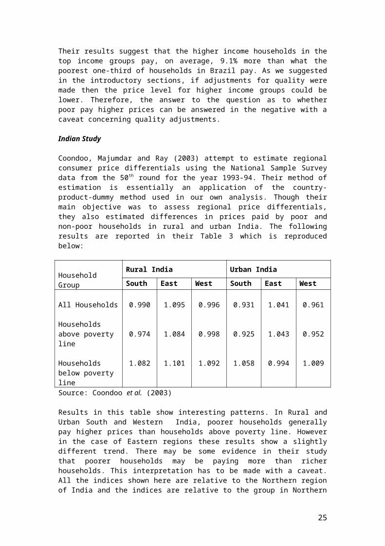
Table A.1 cont.


195 Chat 305.343 46034.835196 Mekmoko 45.409 8523.422197 Coffee whole 92.171 14333.494198 Others 14.628 13063.576199 Salt 18.527 9859.630200 Sugar 102.714 19741.103201 Honey 72.360 5838.203202 Marmalade 58.215 2503.472203 Margarine 49.698 1879.000204 Sugar cane 12.321 24072.289205 Baking powder 19.030 412.050206 Candy and chewing gum 6.257 350.711207 Others 13.503 6170.123208 Mineral water 88.068 22987.878209 Coca Cola Fanta etc 79.696 14170.593210 Birz 44.113 20812.709211 Star O.pop etc 249.311 1335.274212 Others 23.490 7724.436213 Spirit local 215.575 7909.396214 Cognac local 1032.340 31053.500215 Brandy 173.145 5643.000216 Whisky 534.220 4488.750217 Gin local 173.743 4670.333218 Vermouth 1.800 180.000219 Wine 62.414 7821.120220 Katikalla 65.998 9248.833221 Beer 192.757 21229.870222 Tela Borde Korefe 34.157 40871.758223 Mead 75.527 33271.922224 Others 26.388 26043.543225 Nyala 1430.017 6049.158226 Gureza 383.010 3432.000227 Gissila 107.572 1095.822228 Sportsman 944.091 4387.500229 Rothmans 603.109 1522.215230 Craven 102.377 474.000231 Pall mail 237.520 1020.000232 Marlboro 780.178 2070.000233 Winston 257.741 594.857234 Kent 104.250 519.000235 More 8940.000 35760.000236 Peter 79.909 469.263237 Bond 84.934 483.730238 Grusse 129.253 888.095239 Royals 181.878 1105.846240 Sofrudin 136.511 892.071241 Others 115.328 3089.096242 Suret 28.048 1469.095243 Gaye 44.815 3057.140244 Addis club 19.065 600.937245 Others 27.789 2401.187246 Coffee 36.548 3896.490247 Tea 30.394 10664.509248 Milk with Tea or Coffee 38.127 7813.320249 Meal 194.168 14436.031250 Alcoholic Drinks 97.210 6846.025251 Non Alcoholic Drinks 57.592 9487.970252 Others 94.736 8557.867

25

Table A.1 cont.


253 20101 15.010 3960.000254 20112 168.210 37380.000255 30301 152.100 7380000.000256 30401 19.080 1260.000257 41109 1.917 153.333258 41111 3.000 6.000259 41198 .520 105.000260 80117 30.000 1800.000261 80198 21.000 1200.000

Items 253 to 261 represent non-food items. These are too few to be included in the empirical analysis.

26

TABLE A.2 Binary Index Numbers – 10 Income Groups, Ethiopia

Paasche

1.000 1.001 1.078 1.054 1.023 1.014 1.034 1.003 0.993 0.9611.757 1.000 1.625 1.611 1.597 1.602 1.772 1.625 1.513 1.5641.109 1.337 1.000 1.281 0.886 1.043 0.990 1.144 1.012 0.8891.048 1.045 1.012 1.000 1.021 1.019 1.069 1.013 0.984 0.9791.011 1.053 1.001 1.051 1.000 1.025 1.037 1.026 0.975 0.9861.017 1.075 1.035 1.035 1.005 1.000 1.041 1.023 0.946 0.9621.013 1.092 1.030 1.096 0.986 1.045 1.000 1.050 0.996 0.9551.178 1.145 1.029 1.127 1.116 1.097 1.173 1.000 1.059 0.9541.055 1.083 1.045 1.050 1.028 1.042 1.079 1.040 1.000 0.9801.262 1.150 1.060 1.137 1.067 1.093 1.212 1.020 1.050 1.000

Laspeyres

1.000 0.569 0.902 0.955 0.989 0.984 0.987 0.849 0.948 0.7920.999 1.000 0.748 0.957 0.950 0.930 0.916 0.873 0.923 0.8700.928 0.615 1.000 0.989 0.999 0.966 0.971 0.972 0.957 0.9440.948 0.621 0.781 1.000 0.951 0.966 0.912 0.887 0.952 0.8790.978 0.626 1.128 0.980 1.000 0.995 1.015 0.896 0.973 0.9380.986 0.624 0.959 0.982 0.976 1.000 0.957 0.911 0.960 0.9150.967 0.564 1.010 0.936 0.964 0.961 1.000 0.852 0.926 0.8250.997 0.615 0.874 0.987 0.975 0.977 0.952 1.000 0.962 0.9811.007 0.661 0.988 1.016 1.026 1.057 1.004 0.944 1.000 0.9521.041 0.639 1.125 1.021 1.015 1.039 1.047 1.049 1.020 1.000

Fisher

1.000 0.755 0.986 1.003 1.006 0.999 1.010 0.923 0.970 0.8731.325 1.000 1.102 1.242 1.231 1.221 1.274 1.191 1.182 1.1661.014 0.907 1.000 1.125 0.941 1.004 0.980 1.055 0.984 0.9160.997 0.805 0.889 1.000 0.985 0.992 0.987 0.948 0.968 0.9280.994 0.812 1.063 1.015 1.000 1.010 1.026 0.959 0.974 0.9611.001 0.819 0.996 1.008 0.990 1.000 0.998 0.966 0.953 0.9380.990 0.785 1.020 1.013 0.975 1.002 1.000 0.946 0.960 0.8881.084 0.840 0.948 1.055 1.043 1.036 1.057 1.000 1.009 0.9671.031 0.846 1.016 1.033 1.027 1.049 1.041 0.991 1.000 0.9661.146 0.857 1.092 1.078 1.040 1.066 1.126 1.034 1.035 1.000

Tornqvist

1.000 1.000 0.981 1.019 0.999 1.019 0.991 1.004 0.993 0.9781.000 1.000 0.998 1.002 0.992 1.001 0.990 0.986 0.972 0.9661.019 1.002 1.000 0.997 0.939 0.996 0.968 0.990 0.986 0.9280.981 0.998 1.003 1.000 0.983 1.002 0.989 0.982 0.970 0.9531.001 1.008 1.065 1.018 1.000 1.021 1.013 0.991 0.983 0.9780.981 0.999 1.004 0.998 0.979 1.000 0.987 0.989 0.960 0.9531.009 1.010 1.033 1.011 0.987 1.013 1.000 0.999 0.994 0.9740.996 1.014 1.010 1.019 1.009 1.011 1.001 1.000 0.986 0.9761.007 1.029 1.014 1.031 1.017 1.041 1.006 1.014 1.000 0.9841.022 1.035 1.077 1.049 1.023 1.049 1.026 1.025 1.017 1.000

27

TABLE A.3 EKS Distances

Paasche-Laspeyres Spread

0.00000.5644 0.00000.1779 0.7759 0.00000.0995 0.5206 0.2591 0.00000.0333 0.5197 0.1194 0.0707 0.00000.0306 0.5435 0.0766 0.0526 0.0291 0.00000.0461 0.6597 0.0195 0.1584 0.0219 0.0843 0.00000.1675 0.6212 0.1628 0.1326 0.1358 0.1158 0.2087 0.00000.0465 0.4937 0.0560 0.0332 0.0023 0.0146 0.0721 0.0963 0.00000.1932 0.5870 0.0599 0.1074 0.0501 0.0510 0.1458 0.0281 0.0287 0.0000

Quantity Correlations

1.00000.90599 1.00000.84283 0.90580 1.00000.83939 0.91595 0.90810 1.00000.79685 0.88474 0.88784 0.93613 1.00000.62163 0.71679 0.74109 0.76102 0.77221 1.00000.75045 0.84317 0.86437 0.90883 0.91955 0.85222 1.00000.75325 0.83732 0.83612 0.90595 0.92709 0.81032 0.96419 1.00000.70134 0.79552 0.79021 0.85167 0.88115 0.72122 0.92624 0.94318 1.00000.79290 0.82758 0.83410 0.88340 0.87751 0.69187 0.85836 0.86605 0.87100 1.0000

28

TABLE A.4 CPD Regressions Using Unit Record Data – 10 Income Groups, Ethiopia

Model K Model L Model M Model N Model O Model PCoef. St. Err Coef. St. Err Coef. St. Err Coef. St. Err Coef. St. Err Coef.

St. Err

Income Group Dummies

2 -0.0026 0.0012 -0.0027 0.0012 -0.0024 0.0012 -0.0016 0.0010 -0.0019 0.0010-0.0026 0.00103 -0.0027 0.0012 -0.0030 0.0012 -0.0011 0.0012 -0.0018 0.0010 -0.0024 0.0010-0.0033 0.00104 -0.0037 0.0012 -0.0040 0.0012 -0.0035 0.0012 0.0021 0.0010 0.0012 0.0010-0.0004 0.00105 -0.0026 0.0012 -0.0030 0.0012 -0.0034 0.0012 0.0051 0.0010 0.0039 0.0010 0.00080.00106 0.0010 0.0012 0.0005 0.0013 -0.0014 0.0012 0.0142 0.0010 0.0127 0.0011 0.00680.00107 0.0099 0.0012 0.0092 0.0013 0.0017 0.0012 0.0249 0.0010 0.0231 0.0011 0.01050.00108 0.0048 0.0012 0.0040 0.0013 0.0018 0.0012 0.0212 0.0011 0.0189 0.0011 0.01180.00109 0.0074 0.0012 0.0063 0.0013 0.0060 0.0012 0.0198 0.0011 0.0166 0.0012 0.01210.001010 0.0183 0.0012 0.0156 0.0016 0.0168 0.0012 0.0277 0.0012 0.0210 0.0016 0.01760.0011

Income - - 1.5E-7 5.7E-8 - - - - 4.2E-7 6.8E-8 --

Regional Dummies

2 - - - - -0.0603 0.0018 - - - - -0.04240.00143 - - - - -0.0829 0.0013 - - - - -0.09330.00104 - - - - -0.1466 0.0012 - - - - -0.13780.00105 - - - - 0.0931 0.0017 - - - - 0.03760.00146 - - - - -0.0806 0.0015 - - - - -0.10450.00137 - - - - -0.1364 0.0013 - - - - -0.10640.00118 - - - - -0.0157 0.0017 - - - - -0.05020.00159 - - - - -0.0098 0.0016 - - - - 0.02600.001410 - - - - -0.0918 0.0014 - - - - -0.06440.001211 - - - - 0.0357 0.0016 - - - - 0.11820.0013

ProductDummies

1 -5.7473 0.0192 -5.7474 0.0192 -5.6947 0.0184 -5.7549 0.0116 -5.7553 0.0116-5.7337 0.01102 -6.1383 0.0180 -6.1384 0.0180 -6.0562 0.0172 -6.1464 0.0119 -6.1465 0.0119-6.0675 0.01123 -5.8777 0.0187 -5.8777 0.0187 -5.8022 0.0179 -5.8788 0.0107 -5.8788 0.0107-5.8130 0.01014 -6.0209 0.0028 -6.0210 0.0028 -5.9219 0.0028 -6.0373 0.0027 -6.0374 0.0027-5.9419 0.00275 -6.0800 0.0041 -6.0800 0.0041 -6.0297 0.0040 -6.0728 0.0040 -6.0729 0.0040-6.0337 0.00386 -6.1018 0.0074 -6.1018 0.0074 -6.0269 0.0071 -6.1025 0.0076 -6.1027 0.0076-6.0421 0.00727 -6.0168 0.0043 -6.0169 0.0043 -5.9130 0.0042 -6.0411 0.0043 -6.0413 0.0043-5.9343 0.00418 -6.0603 0.0068 -6.0604 0.0068 -5.9529 0.0066 -6.0631 0.0064 -6.0633 0.0064-5.9580 0.0061

29

9 -6.1232 0.0075 -6.1232 0.0075 -6.0047 0.0073 -6.1259 0.0076 -6.1261 0.0076-6.0101 0.007210 -6.2099 0.0374 -6.2099 0.0374 -6.0942 0.0358 -6.2321 0.0358 -6.2322 0.0358-6.1177 0.033711 -6.0170 0.0186 -6.0170 0.0186 -5.9573 0.0178 -6.0397 0.0137 -6.0399 0.0137-5.9604 0.012912 -6.4558 0.0022 -6.4559 0.0022 -6.3651 0.0024 -6.4625 0.0019 -6.4626 0.0019-6.3718 0.002013 -6.3122 0.0120 -6.3123 0.0120 -6.2121 0.0115 -6.3427 0.0121 -6.3429 0.0121-6.2441 0.011414 -6.1982 0.0036 -6.1983 0.0036 -6.1539 0.0036 -6.1729 0.0033 -6.1730 0.0033-6.1536 0.003215 -6.3903 0.0229 -6.3903 0.0229 -6.3107 0.0219 -6.3428 0.0224 -6.3430 0.0224-6.2598 0.021016 -5.3094 0.0038 -5.3095 0.0038 -5.2886 0.0038 -5.3232 0.0041 -5.3233 0.0041-5.3318 0.003917 -5.6111 0.0093 -5.6113 0.0093 -5.5454 0.0090 -5.6764 0.0137 -5.6766 0.0137-5.5901 0.012918 -5.8482 0.0255 -5.8482 0.0255 -5.7368 0.0244 -5.8864 0.0345 -5.8866 0.0345-5.7748 0.032519 -6.3421 0.0506 -6.3421 0.0506 -6.2155 0.0484 -6.3633 0.0484 -6.3633 0.0484-6.2595 0.045520 -6.8255 0.0037 -6.8255 0.0037 -6.7188 0.0037 -6.8675 0.0029 -6.8677 0.0029-6.7701 0.002921 -6.9274 0.0106 -6.9275 0.0106 -6.7898 0.0102 -6.9411 0.0136 -6.9413 0.0136-6.8169 0.012922 -5.9317 0.0067 -5.9318 0.0067 -5.8704 0.0065 -5.9504 0.0092 -5.9505 0.0092-5.8737 0.008723 -5.7207 0.0034 -5.7208 0.0034 -5.6397 0.0034 -5.7264 0.0016 -5.7267 0.0016-5.6490 0.001724 -5.9202 0.0026 -5.9202 0.0026 -5.8307 0.0027 -5.9123 0.0012 -5.9124 0.0012-5.8286 0.001425 -5.8808 0.0028 -5.8809 0.0028 -5.7907 0.0029 -5.8723 0.0013 -5.8724 0.0013-5.7903 0.001526 -5.9651 0.0023 -5.9652 0.0023 -5.8860 0.0024 -5.9839 0.0015 -5.9840 0.0015-5.9029 0.001627 -6.0792 0.0033 -6.0792 0.0033 -6.0419 0.0032 -6.0884 0.0020 -6.0886 0.0020-6.0584 0.002028 -6.0796 0.0053 -6.0796 0.0053 -6.0096 0.0052 -6.0848 0.0039 -6.0849 0.0039-6.0164 0.003729 -6.0171 0.0041 -6.0172 0.0041 -5.9234 0.0040 -6.0193 0.0027 -6.0194 0.0027-5.9260 0.002730 -6.0579 0.0077 -6.0579 0.0077 -5.9449 0.0074 -6.0442 0.0052 -6.0443 0.0052-5.9334 0.005031 -5.9531 0.0242 -5.9532 0.0242 -5.8388 0.0231 -6.1687 0.0219 -6.1686 0.0219-6.0369 0.020632 -6.0895 0.0182 -6.0895 0.0182 -6.0487 0.0174 -6.1118 0.0084 -6.1118 0.0084-6.0722 0.007933 -6.2506 0.0020 -6.2507 0.0020 -6.1716 0.0022 -6.2176 0.0012 -6.2177 0.0012-6.1442 0.0014

30

Table A.4 cont.


St. Err

34 -6.3205 0.0058 -6.3206 0.0058 -6.2157 0.0056 -6.3045 0.0036 -6.3046 0.0036-6.2031 0.003535 -6.2096 0.0024 -6.2096 0.0024 -6.1462 0.0025 -6.2099 0.0012 -6.2100 0.0012-6.1566 0.001436 -6.4863 0.0047 -6.4864 0.0047 -6.4011 0.0046 -6.5144 0.0026 -6.5145 0.0026-6.4200 0.002637 -6.0344 0.0161 -6.0344 0.0161 -5.9833 0.0154 -6.0274 0.0092 -6.0276 0.0092-6.0010 0.008738 -6.1081 0.0184 -6.1082 0.0184 -6.0205 0.0176 -6.0985 0.0094 -6.0987 0.0094-6.0093 0.008939 -6.1391 0.0119 -6.1391 0.0119 -6.0778 0.0114 -6.1217 0.0103 -6.1218 0.0103-6.0759 0.009740 -6.1723 0.0264 -6.1723 0.0264 -6.0978 0.0253 -6.0951 0.0117 -6.0952 0.0117-5.9830 0.011041 -5.2822 0.0074 -5.2822 0.0074 -5.1850 0.0072 -5.1996 0.0066 -5.1997 0.0066-5.0903 0.006342 -6.0591 0.0097 -6.0592 0.0097 -5.9671 0.0093 -5.9772 0.0062 -5.9773 0.0062-5.8839 0.005943 -5.4151 0.0045 -5.4152 0.0045 -5.3720 0.0044 -5.4242 0.0040 -5.4243 0.0040-5.3796 0.003844 -6.1861 0.0448 -6.1862 0.0448 -6.0719 0.0428 -6.0919 0.0286 -6.0920 0.0286-5.9903 0.026945 -5.6559 0.0125 -5.6559 0.0125 -5.6259 0.0120 -5.2302 0.0110 -5.2303 0.0110-5.1938 0.010446 -5.3066 0.0225 -5.3067 0.0225 -5.2144 0.0216 -5.4085 0.0290 -5.4091 0.0290-5.3352 0.027347 -6.2517 0.0059 -6.2518 0.0059 -6.1947 0.0057 -6.2608 0.0039 -6.2610 0.0039-6.2148 0.003748 -5.8292 0.0035 -5.8292 0.0035 -5.7224 0.0035 -5.8470 0.0039 -5.8471 0.0039-5.7423 0.003849 -5.9253 0.0029 -5.9254 0.0029 -5.8258 0.0030 -5.9582 0.0035 -5.9583 0.0035-5.8582 0.003450 -5.7406 0.0064 -5.7406 0.0064 -5.6371 0.0062 -5.7516 0.0089 -5.7518 0.0089-5.6580 0.008451 -5.4176 0.0040 -5.4177 0.0040 -5.3378 0.0039 -5.4270 0.0063 -5.4272 0.0063-5.3570 0.006052 -6.1398 0.0050 -6.1398 0.0050 -6.0346 0.0049 -6.1183 0.0050 -6.1184 0.0050-6.0093 0.004853 -5.7404 0.0156 -5.7404 0.0156 -5.6230 0.0149 -5.7864 0.0217 -5.7865 0.0217-5.6779 0.020454 -6.1303 0.0157 -6.1303 0.0157 -6.0203 0.0150 -6.1813 0.0214 -6.1814 0.0214-6.0652 0.020255 -5.4734 0.0045 -5.4735 0.0045 -5.3673 0.0044 -5.4622 0.0152 -5.4624 0.0152-5.3518 0.014356 -6.0394 0.0035 -6.0394 0.0035 -5.9398 0.0035 -5.8961 0.0029 -5.8962 0.0029-5.8005 0.002957 -6.1371 0.0173 -6.1371 0.0173 -6.0543 0.0165 -6.1364 0.0149 -6.1365 0.0149-6.0397 0.014158 -6.4808 0.0106 -6.4808 0.0106 -6.3735 0.0102 -6.5304 0.0147 -6.5305 0.0147-6.4241 0.013959 -5.1993 0.0029 -5.1993 0.0029 -5.0998 0.0029 -5.1314 0.0024 -5.1316 0.0024-5.0371 0.002460 -5.3245 0.0062 -5.3246 0.0062 -5.2459 0.0059 -5.3342 0.0063 -5.3343 0.0063-5.2443 0.006061 -5.1872 0.0026 -5.1873 0.0026 -5.1044 0.0026 -5.1886 0.0027 -5.1888 0.0027-5.1111 0.002762 -5.2171 0.0031 -5.2171 0.0031 -5.1457 0.0032 -5.1968 0.0034 -5.1970 0.0034-5.1274 0.003363 -5.3076 0.0029 -5.3076 0.0029 -5.2226 0.0029 -5.2812 0.0025 -5.2813 0.0025-5.2007 0.002564 -5.2155 0.0028 -5.2156 0.0028 -5.1319 0.0029 -5.2200 0.0032 -5.2202 0.0032-5.1356 0.003265 -5.0705 0.0024 -5.0705 0.0024 -4.9825 0.0025 -5.0736 0.0030 -5.0738 0.0030-4.9925 0.002966 -5.4102 0.0036 -5.4102 0.0036 -5.3275 0.0035 -5.4062 0.0033 -5.4063 0.0033-5.3159 0.003267 -5.5707 0.0105 -5.5707 0.0105 -5.4824 0.0101 -5.5750 0.0109 -5.5751 0.0109-5.4817 0.0103

31

68 -6.1967 0.0078 -6.1967 0.0078 -6.1082 0.0075 -6.2227 0.0084 -6.2229 0.0084-6.1104 0.008069 -5.5649 0.0073 -5.5649 0.0073 -5.4844 0.0071 -5.5925 0.0063 -5.5926 0.0063-5.5046 0.006070 -5.5049 0.0188 -5.5050 0.0188 -5.4463 0.0180 -5.4793 0.0303 -5.4794 0.0303-5.4230 0.028571 -4.9020 0.0033 -4.9020 0.0033 -4.8558 0.0033 -4.9549 0.0052 -4.9550 0.0052-4.9494 0.005072 -6.0791 0.0111 -6.0792 0.0111 -5.9865 0.0107 -6.0810 0.0115 -6.0811 0.0115-5.9703 0.010973 -5.9221 0.0072 -5.9222 0.0072 -5.8370 0.0069 -5.9052 0.0088 -5.9054 0.0088-5.8081 0.008374 -5.3277 0.0068 -5.3277 0.0068 -5.2378 0.0066 -5.3077 0.0120 -5.3079 0.0120-5.2142 0.011475 -5.3294 0.0180 -5.3294 0.0180 -5.2615 0.0173 -5.1230 0.0250 -5.1232 0.0250-5.0200 0.023576 -5.3496 0.0041 -5.3496 0.0041 -5.2865 0.0040 -5.3872 0.0083 -5.3874 0.0083-5.3288 0.007977 -5.2451 0.0074 -5.2451 0.0074 -5.1708 0.0072 -5.2349 0.0124 -5.2351 0.0124-5.1463 0.011778 -5.7057 0.0086 -5.7057 0.0086 -5.6121 0.0083 -5.7039 0.0114 -5.7040 0.0114-5.6110 0.010879 -5.7941 0.0282 -5.7942 0.0282 -5.6967 0.0270 -5.6558 0.0983 -5.6560 0.0983-5.5605 0.092580 -5.6470 0.0063 -5.6470 0.0063 -5.5563 0.0061 -5.6498 0.0220 -5.6500 0.0220-5.5506 0.020781 -5.5732 0.0262 -5.5732 0.0262 -5.4876 0.0251 -5.5675 0.0683 -5.5677 0.0683-5.4726 0.064282 -5.0592 0.0041 -5.0594 0.0041 -5.0076 0.0040 -5.0513 0.0052 -5.0516 0.0052-5.0267 0.005083 -4.9672 0.0107 -4.9673 0.0107 -4.8873 0.0103 -4.9337 0.0194 -4.9339 0.0194-4.8778 0.018384 -5.2327 0.0034 -5.2327 0.0034 -5.1651 0.0034 -5.2418 0.0047 -5.2420 0.0047-5.1922 0.004585 -5.1314 0.0320 -5.1314 0.0320 -5.0497 0.0306 -5.1258 0.0504 -5.1260 0.0504-5.0376 0.047486 -5.0552 0.0521 -5.0555 0.0521 -4.9900 0.0498 -5.1500 0.0548 -5.1503 0.0548-5.1542 0.051587 -4.9986 0.0188 -4.9986 0.0188 -4.9925 0.0180 -4.9241 0.0240 -4.9240 0.0240-4.9285 0.022688 -6.0901 0.0028 -6.0902 0.0028 -6.0067 0.0029 -6.0972 0.0015 -6.0974 0.0015-6.0325 0.001789 -6.1905 0.0032 -6.1906 0.0032 -6.1025 0.0032 -6.1946 0.0028 -6.1948 0.0028-6.1226 0.002790 -5.5676 0.0022 -5.5676 0.0022 -5.4990 0.0023 -5.5572 0.0018 -5.5574 0.0018-5.5134 0.001991 -4.7733 0.0199 -4.7737 0.0199 -4.6890 0.0190 -4.8614 0.0268 -4.8626 0.0268-4.8123 0.025292 -4.7213 0.0068 -4.7214 0.0068 -4.6554 0.0066 -4.7251 0.0131 -4.7256 0.0131-4.6858 0.012493 -5.7734 0.0083 -5.7735 0.0083 -5.6806 0.0080 -5.7581 0.0076 -5.7582 0.0076-5.6676 0.007294 -4.5072 0.0022 -4.5072 0.0022 -4.4286 0.0023 -4.5124 0.0015 -4.5127 0.0015-4.4364 0.001695 -4.6064 0.0055 -4.6066 0.0055 -4.5206 0.0054 -4.5920 0.0029 -4.5925 0.0029-4.4967 0.002996 -4.7172 0.0042 -4.7174 0.0042 -4.6383 0.0042 -4.7276 0.0045 -4.7278 0.0045-4.6444 0.004397 -3.8010 0.0304 -3.8012 0.0304 -3.7633 0.0291 -3.8302 0.0114 -3.8304 0.0114-3.7665 0.010898 -3.9518 0.0877 -3.9519 0.0877 -3.9046 0.0838 -3.8580 0.0493 -3.8581 0.0493-3.7634 0.0464

32

Table A.4 cont.


St. Err

99 -4.6763 0.0067 -4.6763 0.0067 -4.6331 0.0065 -4.6143 0.0040 -4.6146 0.0040-4.5388 0.0038100 -4.6809 0.0127 -4.6809 0.0127 -4.7098 0.0122 -4.6665 0.0111 -4.6667 0.0111-4.6687 0.0105101 -4.8035 0.0596 -4.8035 0.0596 -4.6959 0.0569 -4.4837 0.0608 -4.4839 0.0608-4.3729 0.0572102 -5.1148 0.0143 -5.1149 0.0143 -5.0472 0.0137 -4.9741 0.0113 -4.9743 0.0113-4.8963 0.0107103 -5.7021 0.0071 -5.7021 0.0071 -5.6395 0.0069 -5.7382 0.0042 -5.7382 0.0042-5.6737 0.0042104 -3.0978 0.0469 -3.0984 0.0469 -3.0737 0.0448 -3.0508 0.0431 -3.0510 0.0431-3.0240 0.0405105 -4.0954 0.1074 -4.0981 0.1074 -4.0993 0.1026 -4.1043 0.1903 -4.1059 0.1903-4.1660 0.1790106 -5.3721 0.0150 -5.3721 0.0150 -5.3242 0.0144 -5.4221 0.0156 -5.4221 0.0156-5.3528 0.0148107 -5.7896 0.0521 -5.7897 0.0521 -5.6875 0.0498 -5.3231 0.1154 -5.3233 0.1154-5.2258 0.1086108 -6.0323 0.0026 -6.0324 0.0026 -5.9701 0.0027 -5.9976 0.0016 -5.9977 0.0017-5.9550 0.0018109 -3.2711 0.0170 -3.2714 0.0170 -3.2295 0.0163 -3.2228 0.0097 -3.2231 0.0097-3.1992 0.0092110 -5.3781 0.0053 -5.3782 0.0053 -5.2539 0.0051 -5.3772 0.0053 -5.3773 0.0053-5.2644 0.0051111 -5.7449 0.0060 -5.7450 0.0060 -5.6493 0.0059 -5.6002 0.0053 -5.6004 0.0053-5.5268 0.0051112 -6.7424 0.0045 -6.7424 0.0045 -6.6285 0.0044 -6.7453 0.0043 -6.7454 0.0043-6.6377 0.0042113 -1.0611 0.0035 -1.0612 0.0035 -0.9763 0.0035 -1.0728 0.0052 -1.0742 0.0052-0.9892 0.0049114 -6.1351 0.0135 -6.1351 0.0135 -6.0441 0.0130 -5.5386 0.0112 -5.5388 0.0112-5.4655 0.0106115 -3.7813 0.0029 -3.7814 0.0029 -3.6694 0.0030 -3.8004 0.0032 -3.8006 0.0032-3.6901 0.0032116 -3.7063 0.0052 -3.7065 0.0052 -3.6154 0.0051 -3.7164 0.0069 -3.7167 0.0069-3.6244 0.0066117 -4.0086 0.0230 -4.0090 0.0230 -3.9388 0.0220 -3.9743 0.0244 -3.9749 0.0244-3.9315 0.0229118 -4.1686 0.0021 -4.1686 0.0021 -4.0644 0.0022 -4.1646 0.0016 -4.1648 0.0016-4.0658 0.0017119 -4.3873 0.0026 -4.3874 0.0026 -4.3642 0.0027 -4.3991 0.0021 -4.3993 0.0021-4.3820 0.0021120 -3.9974 0.0161 -3.9974 0.0161 -3.9082 0.0154 -4.0511 0.0218 -4.0511 0.0218-3.9442 0.0205121 -7.4189 0.0019 -7.4190 0.0019 -7.3117 0.0021 -7.4604 0.0023 -7.4605 0.0023-7.3558 0.0023122 -6.8669 0.0036 -6.8670 0.0036 -6.7841 0.0036 -6.8895 0.0081 -6.8898 0.0081-6.8102 0.0077123 -6.4438 0.0061 -6.4439 0.0061 -6.3988 0.0059 -6.3679 0.0165 -6.3679 0.0165-6.3141 0.0156124 -6.9987 0.0052 -6.9989 0.0052 -6.9484 0.0050 -6.9708 0.0126 -6.9710 0.0126-6.9365 0.0119125 -6.2416 0.0041 -6.2417 0.0041 -6.1621 0.0041 -6.1878 0.0112 -6.1882 0.0112-6.1249 0.0106126 -5.9797 0.0023 -5.9798 0.0023 -5.9210 0.0024 -5.9555 0.0034 -5.9557 0.0034-5.9207 0.0033127 -5.5582 0.0018 -5.5583 0.0018 -5.4800 0.0020 -5.5461 0.0018 -5.5463 0.0018-5.4738 0.0019128 -4.9648 0.0022 -4.9649 0.0022 -4.8824 0.0024 -4.8902 0.0043 -4.8904 0.0043-4.8180 0.0042129 -5.6651 0.0020 -5.6652 0.0020 -5.5739 0.0021 -5.6852 0.0049 -5.6853 0.0049-5.5921 0.0047130 -7.1684 0.0041 -7.1685 0.0041 -7.0935 0.0041 -7.1076 0.0068 -7.1077 0.0068-7.0433 0.0064131 -6.1533 0.0159 -6.1537 0.0159 -6.0572 0.0152 -5.9708 0.0179 -5.9710 0.0179-5.8780 0.0168132 -6.6835 0.0042 -6.6836 0.0042 -6.5928 0.0041 -6.6921 0.0114 -6.6923 0.0114-6.6041 0.0108

33

133 -6.1985 0.0358 -6.1986 0.0358 -6.1141 0.0342 -6.2684 0.0284 -6.2689 0.0284-6.2136 0.0267134 -5.9849 0.0163 -5.9850 0.0163 -5.8747 0.0157 -5.8968 0.0108 -5.8969 0.0108-5.7837 0.0102135 -4.1819 0.0066 -4.1820 0.0066 -4.1932 0.0064 -4.1870 0.0128 -4.1874 0.0128-4.1888 0.0121136 -6.3956 0.0052 -6.3957 0.0052 -6.3154 0.0051 -6.3871 0.0100 -6.3874 0.0100-6.2851 0.0094137 -6.8847 0.0156 -6.8847 0.0156 -6.7783 0.0150 -6.8467 0.0235 -6.8468 0.0235-6.7378 0.0221138 -7.4334 0.0082 -7.4334 0.0082 -7.2972 0.0079 -7.4541 0.0078 -7.4543 0.0078-7.3452 0.0074139 -6.3401 0.0050 -6.3401 0.0050 -6.2018 0.0049 -6.3381 0.0084 -6.3383 0.0084-6.2173 0.0079140 -6.8682 0.0045 -6.8682 0.0045 -6.7909 0.0045 -6.8950 0.0049 -6.8952 0.0049-6.8194 0.0047141 -6.3801 0.0041 -6.3802 0.0041 -6.2778 0.0041 -6.3418 0.0077 -6.3420 0.0077-6.2490 0.0073142 -6.1076 0.0055 -6.1078 0.0055 -6.0148 0.0053 -6.0893 0.0115 -6.0898 0.0115-6.0056 0.0109143 -5.9155 0.0053 -5.9156 0.0053 -5.8544 0.0052 -5.8767 0.0307 -5.8769 0.0307-5.8363 0.0289144 -6.0805 0.0374 -6.0804 0.0374 -6.0045 0.0357 -6.0963 0.0716 -6.0954 0.0716-6.0374 0.0674145 -6.0547 0.0331 -6.0547 0.0331 -5.9927 0.0317 -6.0550 0.1070 -6.0554 0.1070-6.0240 0.1007146 -6.1912 0.0102 -6.1913 0.0102 -6.0543 0.0098 -6.2021 0.0212 -6.2023 0.0211-6.0863 0.0199147 -5.8769 0.0812 -5.8766 0.0812 -5.7761 0.0776 -5.2797 0.3014 -5.2794 0.3014-5.1953 0.2835148 -5.7198 0.0413 -5.7199 0.0413 -5.6411 0.0395 -6.0481 0.0594 -6.0483 0.0594-6.0589 0.0559149 -6.3450 0.0119 -6.3450 0.0119 -6.3122 0.0114 -5.4887 0.0048 -5.4887 0.0048-5.4819 0.0046150 -6.9919 0.0084 -6.9919 0.0084 -6.9038 0.0081 -6.7960 0.0155 -6.7962 0.0155-6.7132 0.0146151 -5.4118 0.0812 -5.4116 0.0812 -5.3017 0.0776 -5.3416 0.1735 -5.3414 0.1735-5.2484 0.1632152 -6.1278 0.0266 -6.1280 0.0266 -6.0079 0.0255 -5.9002 0.0551 -5.9004 0.0551-5.8029 0.0519153 -6.9070 0.0163 -6.9070 0.0163 -6.8099 0.0157 -6.8136 0.0557 -6.8137 0.0557-6.7507 0.0524154 -6.4042 0.0066 -6.4043 0.0066 -6.3557 0.0064 -6.2266 0.0084 -6.2268 0.0084-6.1783 0.0079155 -6.7518 0.1240 -6.7551 0.1240 -6.6681 0.1185 -6.7035 0.2961 -6.7046 0.2961-6.6475 0.2785156 -7.0267 0.1518 -7.0268 0.1518 -6.9464 0.1451 -7.2934 0.3698 -7.2934 0.3698-7.1576 0.3478157 -5.4608 0.0200 -5.4612 0.0200 -5.4226 0.0191 -5.6466 0.0181 -5.6468 0.0181-5.6006 0.0170158 -5.0567 0.0112 -5.0568 0.0112 -4.9919 0.0108 -5.0754 0.0207 -5.0755 0.0207-5.0278 0.0195159 -4.9741 0.0506 -4.9748 0.0506 -4.8857 0.0484 -4.9066 0.0952 -4.9072 0.0952-4.8472 0.0895160 -6.3165 0.0421 -6.3172 0.0421 -6.2296 0.0403 -6.3417 0.1119 -6.3423 0.1119-6.2430 0.1052161 -6.3140 0.0141 -6.3142 0.0141 -6.2422 0.0135 -6.0613 0.0181 -6.0615 0.0181-5.9966 0.0170162 -4.2800 0.0049 -4.2800 0.0049 -4.1890 0.0048 -4.3004 0.0060 -4.3005 0.0060-4.2110 0.0058163 -4.2024 0.0017 -4.2025 0.0017 -4.1231 0.0019 -4.2030 0.0014 -4.2032 0.0014-4.1313 0.0015

34

Table A.4 cont.


St. Err

164 -4.3398 0.0098 -4.3399 0.0098 -4.2682 0.0095 -4.3355 0.0224 -4.3359 0.0224-4.2608 0.0211165 -4.0999 0.0092 -4.0999 0.0092 -4.0168 0.0088 -3.9961 0.0279 -3.9962 0.0279-3.9497 0.0263166 -4.6740 0.0042 -4.6741 0.0042 -4.5738 0.0042 -4.6874 0.0207 -4.6875 0.0207-4.5833 0.0195167 -4.6283 0.0040 -4.6284 0.0040 -4.5235 0.0040 -4.6327 0.0174 -4.6327 0.0174-4.5266 0.0164168 -4.5002 0.0026 -4.5003 0.0026 -4.3935 0.0027 -4.4999 0.0040 -4.5001 0.0040-4.3874 0.0039169 -3.4332 0.0074 -3.4333 0.0074 -3.3275 0.0071 -3.1969 0.0138 -3.1971 0.0138-3.1025 0.0130170 -3.2327 0.0107 -3.2328 0.0107 -3.1339 0.0103 -3.1343 0.0325 -3.1344 0.0325-3.0423 0.0306171 -3.9225 0.0043 -3.9226 0.0043 -3.8303 0.0042 -3.9128 0.0138 -3.9129 0.0138-3.8136 0.0130172 -5.0144 0.0025 -5.0145 0.0025 -4.9248 0.0026 -5.0117 0.0123 -5.0119 0.0123-4.9372 0.0116173 -4.6800 0.0203 -4.6804 0.0203 -4.6115 0.0194 -4.9282 0.0312 -4.9289 0.0312-4.8959 0.0293174 -5.6708 0.0051 -5.6709 0.0051 -5.5667 0.0050 -5.7930 0.0222 -5.7932 0.0222-5.6897 0.0209175 -5.4809 0.0062 -5.4810 0.0062 -5.3828 0.0060 -5.5794 0.0300 -5.5795 0.0300-5.4782 0.0282176 -5.5222 0.0105 -5.5222 0.0105 -5.4240 0.0101 -5.6820 0.0642 -5.6821 0.0642-5.5860 0.0603177 -5.6601 0.0151 -5.6602 0.0151 -5.5575 0.0145 -5.4511 0.0726 -5.4513 0.0726-5.3656 0.0683178 -4.3295 0.0033 -4.3295 0.0033 -4.2256 0.0033 -4.2950 0.0048 -4.2952 0.0048-4.1932 0.0046179 -4.8533 0.0040 -4.8533 0.0040 -4.7618 0.0039 -4.6940 0.0140 -4.6942 0.0140-4.5966 0.0132180 -3.4549 0.0185 -3.4550 0.0185 -3.4032 0.0177 -3.5550 0.0654 -3.5552 0.0654-3.5226 0.0615181 -4.4840 0.0040 -4.4841 0.0040 -4.4114 0.0040 -4.4870 0.0079 -4.4871 0.0079-4.4206 0.0075182 -6.6164 0.0020 -6.6164 0.0020 -6.5324 0.0022 -6.6471 0.0020 -6.6473 0.0020-6.5595 0.0020183 -6.8742 0.0042 -6.8743 0.0042 -6.7746 0.0041 -6.9085 0.0034 -6.9086 0.0034-6.8195 0.0033184 -6.9723 0.0031 -6.9724 0.0031 -6.8366 0.0032 -6.9339 0.0014 -6.9341 0.0014-6.8180 0.0017185 -7.7671 0.0056 -7.7671 0.0056 -7.6290 0.0055 -7.7748 0.0053 -7.7750 0.0053-7.6627 0.0051186 -7.0414 0.0127 -7.0415 0.0127 -6.9056 0.0122 -7.0645 0.0208 -7.0645 0.0208-6.9412 0.0196187 -7.5859 0.0064 -7.5860 0.0064 -7.4605 0.0062 -7.5949 0.0061 -7.5950 0.0061-7.4868 0.0058188 -6.6247 0.0115 -6.6248 0.0115 -6.4894 0.0110 -6.6259 0.0099 -6.6261 0.0099-6.5143 0.0094189 -5.7924 0.0076 -5.7927 0.0076 -5.6659 0.0074 -5.8797 0.0107 -5.8800 0.0107-5.7707 0.0101190 -7.2459 0.0097 -7.2459 0.0097 -7.1646 0.0093 -7.0336 0.0093 -7.0338 0.0093-6.9503 0.0088191 -3.9336 0.0021 -3.9337 0.0021 -3.8707 0.0023 -3.9375 0.0037 -3.9377 0.0037-3.8920 0.0036192 -4.3745 0.0017 -4.3745 0.0017 -4.2880 0.0019 -4.3814 0.0014 -4.3815 0.0014-4.2972 0.0016193 -5.8140 0.0041 -5.8141 0.0041 -5.7183 0.0041 -5.8651 0.0045 -5.8652 0.0045-5.7602 0.0043194 -5.8817 0.0046 -5.8817 0.0046 -5.7912 0.0045 -5.8215 0.0103 -5.8217 0.0103-5.7342 0.0097195 -5.0256 0.0031 -5.0257 0.0031 -4.9812 0.0031 -4.9656 0.0018 -4.9658 0.0018-4.9678 0.0019196 -5.1808 0.0269 -5.1808 0.0269 -5.1296 0.0257 -5.3153 0.0410 -5.3153 0.0410-5.2370 0.0385197 -5.0492 0.0038 -5.0493 0.0038 -4.9196 0.0038 -5.0450 0.0031 -5.0451 0.0031-4.9224 0.0030

35

198 -6.6884 0.0041 -6.6884 0.0041 -6.6414 0.0041 -6.7486 0.0079 -6.7488 0.0079-6.6913 0.0075199 -6.2856 0.0015 -6.2856 0.0015 -6.2078 0.0018 -6.2601 0.0025 -6.2602 0.0025-6.1741 0.0025200 -5.2166 0.0019 -5.2166 0.0019 -5.1548 0.0020 -5.2629 0.0017 -5.2631 0.0017-5.2294 0.0018201 -4.3376 0.0084 -4.3377 0.0084 -4.2575 0.0081 -4.3677 0.0096 -4.3679 0.0096-4.2941 0.0091202 -3.9461 0.0295 -3.9468 0.0295 -3.8622 0.0282 -3.6911 0.0410 -3.6915 0.0410-3.6587 0.0385203 -3.6578 0.0421 -3.6583 0.0421 -3.5819 0.0403 -3.5651 0.0435 -3.5653 0.0435-3.4997 0.0409204 -7.5620 0.0049 -7.5620 0.0049 -7.4502 0.0048 -7.5841 0.0117 -7.5843 0.0117-7.4881 0.0111205 -3.2209 0.0086 -3.2209 0.0086 -3.1761 0.0083 -3.0104 0.0175 -3.0107 0.0175-2.9543 0.0165206 -4.0070 0.0068 -4.0071 0.0068 -3.9219 0.0066 -4.0379 0.0268 -4.0381 0.0268-3.9712 0.0252207 -6.0579 0.0122 -6.0581 0.0122 -5.9682 0.0118 -6.1971 0.0282 -6.1973 0.0282-6.1162 0.0265208 -5.6336 0.0095 -5.6342 0.0095 -5.5514 0.0091 -5.5556 0.0149 -5.5568 0.0149-5.4951 0.0140209 -5.1974 0.0073 -5.1978 0.0073 -5.1148 0.0071 -5.1742 0.0110 -5.1751 0.0110-5.1026 0.0104210 -6.1516 0.0212 -6.1517 0.0212 -6.0310 0.0203 -6.1864 0.0320 -6.1867 0.0320-6.0675 0.0301211 -1.6479 0.0117 -1.6481 0.0117 -1.5561 0.0112 -1.6909 0.0096 -1.6920 0.0096-1.5981 0.0091212 -5.6313 0.0164 -5.6317 0.0164 -5.5352 0.0157 -5.4523 0.0292 -5.4526 0.0292-5.3828 0.0274213 -3.6395 0.0295 -3.6399 0.0295 -3.5581 0.0282 -3.5896 0.0190 -3.5897 0.0190-3.4877 0.0179214 -3.5449 0.0620 -3.5449 0.0620 -3.4673 0.0593 -3.5155 0.0233 -3.5158 0.0233-3.3976 0.0219215 -3.4836 0.1518 -3.4837 0.1518 -3.3405 0.1451 -3.4767 0.0946 -3.4769 0.0946-3.3511 0.0890216 -2.1364 0.1074 -2.1377 0.1074 -2.0172 0.1026 -2.0795 0.0866 -2.0800 0.0866-1.9412 0.0815217 -3.4594 0.0716 -3.4610 0.0716 -3.3744 0.0684 -3.3959 0.0654 -3.3964 0.0654-3.2944 0.0615218 -4.6026 0.2147 -4.6026 0.2147 -4.5212 0.2052 -4.6103 1.2901 -4.6104 1.2901-4.5015 1.2134219 -4.8577 0.0430 -4.8588 0.0430 -4.7542 0.0411 -4.8595 0.0784 -4.8610 0.0784-4.7718 0.0737220 -4.9505 0.0072 -4.9506 0.0072 -4.8424 0.0069 -4.9559 0.0075 -4.9560 0.0075-4.8424 0.0071221 -4.7074 0.0162 -4.7078 0.0162 -4.6316 0.0155 -4.7199 0.0157 -4.7214 0.0157-4.6651 0.0147222 -7.1209 0.0050 -7.1210 0.0050 -7.0276 0.0049 -7.0752 0.0065 -7.0753 0.0065-6.9840 0.0061223 -6.1081 0.0166 -6.1081 0.0166 -5.9961 0.0159 -6.0270 0.0183 -6.0271 0.0183-5.9284 0.0172224 -6.8948 0.0222 -6.8949 0.0222 -6.7826 0.0212 -7.0398 0.0301 -7.0400 0.0301-6.9404 0.0283225 -1.4956 0.0086 -1.4958 0.0086 -1.3915 0.0083 -1.5012 0.0044 -1.5081 0.0045-1.4289 0.0042226 -2.2046 0.0716 -2.2046 0.0716 -2.1488 0.0684 -2.0270 0.0461 -2.0270 0.0461-1.9579 0.0434227 -2.3185 0.0185 -2.3185 0.0185 -2.1812 0.0177 -2.3266 0.0150 -2.3265 0.0150-2.1986 0.0142228 -1.5853 0.0406 -1.5854 0.0406 -1.5052 0.0388 -1.5583 0.0147 -1.5582 0.0147-1.4500 0.0138

36

Table A.4 cont.


St. Err

229 -1.0861 0.0195 -1.0864 0.0195 -1.0301 0.0187 -1.0024 0.0104 -1.0029 0.0104-0.9534 0.0098230 -1.4033 0.1074 -1.4034 0.1074 -1.3775 0.1026 -1.5595 0.1005 -1.5596 0.1005-1.5635 0.0945231 -1.4111 0.1240 -1.4111 0.1240 -1.3098 0.1185 -1.4941 0.0587 -1.4942 0.0587-1.3655 0.0552232 -0.9204 0.0877 -0.9210 0.0877 -0.8336 0.0838 -0.9318 0.0438 -0.9336 0.0438-0.8769 0.0412233 -0.8317 0.0812 -0.8320 0.0812 -0.7102 0.0776 -0.7993 0.0403 -0.7997 0.0403-0.6900 0.0379234 -1.3425 0.1518 -1.3419 0.1518 -1.3130 0.1451 -1.6247 0.1517 -1.6247 0.1517-1.7336 0.1427235 -1.3837 0.2147 -1.3838 0.2147 -1.3682 0.2052 -1.3847 0.0291 -1.3848 0.0291-1.3335 0.0274236 -1.8173 0.0493 -1.8173 0.0493 -1.7939 0.0471 -1.8111 0.0527 -1.8111 0.0527-1.8223 0.0495237 -1.7466 0.0353 -1.7464 0.0353 -1.7589 0.0338 -1.6866 0.0390 -1.6864 0.0390-1.6810 0.0367238 -1.9285 0.0271 -1.9286 0.0271 -1.9556 0.0259 -1.9396 0.0217 -1.9397 0.0217-2.0248 0.0205239 -1.8102 0.0266 -1.8102 0.0266 -1.8922 0.0255 -1.8202 0.0215 -1.8202 0.0215-1.8541 0.0203240 -1.8747 0.0406 -1.8747 0.0406 -1.7873 0.0388 -1.8980 0.0383 -1.8980 0.0383-1.8372 0.0361241 -2.7471 0.0068 -2.7471 0.0068 -2.7193 0.0066 -2.6244 0.0060 -2.6245 0.0060-2.6266 0.0057242 -3.9818 0.0083 -3.9818 0.0083 -3.9011 0.0080 -3.9067 0.0113 -3.9069 0.0113-3.8384 0.0107243 -4.2758 0.0045 -4.2758 0.0045 -4.2190 0.0044 -4.2048 0.0053 -4.2049 0.0053-4.1415 0.0051244 -3.5180 0.0380 -3.5180 0.0380 -3.4605 0.0363 -2.7909 0.0765 -2.7908 0.0765-2.8397 0.0720245 -4.4397 0.0071 -4.4398 0.0071 -4.3720 0.0069 -4.4011 0.0105 -4.4012 0.0105-4.3391 0.0099246 -4.6761 0.0091 -4.6762 0.0091 -4.5894 0.0087 -4.6819 0.0157 -4.6822 0.0157-4.5941 0.0148247 -5.8642 0.0041 -5.8642 0.0041 -5.7800 0.0040 -5.8710 0.0068 -5.8712 0.0068-5.7906 0.0065248 -5.3287 0.0086 -5.3287 0.0086 -5.2537 0.0083 -5.3369 0.0140 -5.3370 0.0140-5.2807 0.0132249 -4.3124 0.0034 -4.3125 0.0034 -4.2321 0.0034 -4.3199 0.0023 -4.3201 0.0023-4.2480 0.0023250 -4.2578 0.0039 -4.2578 0.0039 -4.1624 0.0039 -4.2672 0.0037 -4.2673 0.0037-4.1685 0.0036251 -5.1107 0.0066 -5.1108 0.0066 -5.0202 0.0064 -5.1193 0.0092 -5.1194 0.0092-5.0349 0.0086252 -4.5074 0.0078 -4.5076 0.0078 -4.4263 0.0076 -4.5148 0.0081 -4.5151 0.0081-4.4343 0.0076

37

TABLE A.5 CPD Regressions Using Average Data – 10 Income Groups Ethiopia

Model Q Model RCoef. St. Err Coef. St. Err

Income GroupDummies

2 -0.0171 0.0164 -0.0086 0.01403 -0.0151 0.0164 -0.0297 0.01284 -0.0100 0.0163 -0.0108 0.01245 0.0069 0.0163 0.0076 0.01246 -0.0190 0.0163 -0.0135 0.01257 -0.0072 0.0164 0.0096 0.01248 0.0152 0.0163 -0.0030 0.01269 0.0149 0.0162 0.0192 0.012510 0.0592 0.0162 0.0382 0.0128

ProductDummies

1 -5.7417 0.0569 -5.7395 0.02602 -6.1078 0.0569 -6.1068 0.03193 -5.8620 0.0569 -5.8476 0.02514 -6.0173 0.0569 -6.0169 0.05205 -6.0798 0.0569 -6.0734 0.05266 -6.0980 0.0569 -6.0939 0.05877 -6.0085 0.0569 -6.0044 0.05468 -6.0515 0.0569 -6.0515 0.05319 -6.1197 0.0569 -6.1200 0.055310 -6.1991 0.0601 -6.2158 0.053311 -5.9953 0.0569 -5.9966 0.041112 -6.4455 0.0569 -6.4416 0.047313 -6.3114 0.0569 -6.3108 0.056014 -6.1845 0.0569 -6.1773 0.051015 -6.3741 0.0569 -6.3414 0.048616 -5.3051 0.0569 -5.3008 0.046417 -5.6011 0.0569 -5.6026 0.066118 -5.8201 0.0569 -5.8096 0.062519 -6.3416 0.0569 -6.3449 0.058020 -6.7805 0.0569 -6.7805 0.042321 -6.9013 0.0569 -6.9068 0.070622 -5.8358 0.0569 -5.8371 0.064223 -5.7195 0.0569 -5.7183 0.020624 -5.9137 0.0569 -5.9121 0.022125 -5.8741 0.0569 -5.8725 0.021026 -5.9574 0.0569 -5.9551 0.032127 -6.0751 0.0569 -6.0738 0.031428 -6.0744 0.0569 -6.0712 0.039229 -6.0044 0.0569 -6.0035 0.036230 -6.0489 0.0569 -6.0458 0.040431 -5.9430 0.0569 -5.9868 0.047832 -6.0655 0.0569 -6.0726 0.026533 -6.2266 0.0569 -6.2200 0.028034 -6.3157 0.0569 -6.3066 0.036835 -6.1815 0.0569 -6.1698 0.023636 -6.4688 0.0569 -6.4670 0.030937 -6.0266 0.0569 -6.0252 0.027838 -6.1038 0.0569 -6.0987 0.028139 -6.1300 0.0569 -6.1338 0.042740 -6.1859 0.0599 -6.1630 0.028141 -5.2702 0.0569 -5.2672 0.045742 -6.0493 0.0569 -6.0420 0.038743 -5.3988 0.0569 -5.3963 0.044744 -6.1582 0.0569 -6.1156 0.043845 -5.4270 0.0569 -5.4355 0.043546 -5.2706 0.0569 -5.2644 0.049947 -6.2129 0.0569 -6.2188 0.035348 -5.8278 0.0569 -5.8255 0.063049 -5.9211 0.0569 -5.9244 0.0611

38

Table 5 cont.


50 -5.7135 0.0569 -5.7149 0.076151 -5.4133 0.0569 -5.4086 0.074552 -6.1188 0.0569 -6.1110 0.055453 -5.7156 0.0569 -5.7163 0.072954 -6.1154 0.0569 -6.1143 0.075255 -5.4635 0.0569 -5.4579 0.184456 -6.0003 0.0569 -5.9986 0.049357 -6.1402 0.0569 -6.1349 0.048658 -6.2779 0.0569 -5.9935 0.066459 -5.1923 0.0569 -5.1866 0.045760 -5.3201 0.0569 -5.3172 0.052761 -5.1836 0.0569 -5.1797 0.052962 -5.2131 0.0569 -5.2068 0.055663 -5.3069 0.0569 -5.3056 0.046464 -5.2119 0.0569 -5.2086 0.054765 -5.0667 0.0569 -5.0655 0.058666 -5.4087 0.0569 -5.4052 0.049867 -5.5646 0.0569 -5.5624 0.058268 -6.1050 0.0569 -6.0942 0.056969 -5.5498 0.0569 -5.5396 0.044270 -5.4618 0.0569 -5.4569 0.074371 -4.8883 0.0569 -4.8913 0.081772 -6.0716 0.0569 -6.0747 0.062373 -5.8664 0.0569 -5.8648 0.069674 -5.3240 0.0569 -5.3176 0.094375 -5.2962 0.0569 -5.3182 0.080376 -5.3406 0.0569 -5.3340 0.104477 -5.2358 0.0569 -5.2354 0.100678 -5.7010 0.0569 -5.6980 0.076179 -5.5281 0.0569 -5.6331 0.212180 -5.6321 0.0569 -5.6301 0.186881 -5.4346 0.0569 -5.3734 0.139782 -5.0481 0.0569 -5.0452 0.052783 -4.9336 0.0569 -4.9320 0.067984 -5.2282 0.0569 -5.2257 0.060985 -5.1236 0.0569 -5.1042 0.067486 -5.0588 0.0634 -5.0533 0.040087 -4.9684 0.0569 -4.9528 0.051788 -6.0708 0.0569 -6.0687 0.028789 -6.1638 0.0569 -6.1583 0.046590 -5.5613 0.0569 -5.5601 0.037991 -4.7790 0.0569 -4.7479 0.044992 -4.7025 0.0569 -4.7010 0.088993 -5.6586 0.0569 -5.6598 0.051394 -4.4977 0.0569 -4.4972 0.029695 -4.5983 0.0569 -4.5965 0.022196 -4.7060 0.0569 -4.7134 0.045897 -3.7872 0.0569 -3.8119 0.021898 -3.9458 0.0732 -3.8979 0.037999 -4.6557 0.0569 -4.6564 0.0271100 -4.6730 0.0569 -4.6712 0.0355101 -4.6957 0.0676 -4.3982 0.0697102 -5.0729 0.0569 -5.0557 0.0447103 -5.6416 0.0569 -5.6552 0.0308104 -3.1784 0.0676 -3.2731 0.0366105 -4.1056 0.0893 -4.0594 0.1053106 -5.3460 0.0569 -5.3583 0.0513107 -5.6991 0.0599 -4.9355 0.0762108 -6.0264 0.0569 -6.0234 0.0324109 -3.2648 0.0569 -3.2427 0.0216110 -5.3608 0.0569 -5.3606 0.0511111 -5.7265 0.0569 -5.7258 0.0464112 -6.7232 0.0569 -6.7236 0.0519113 -1.0564 0.0569 -1.0553 0.0619114 -5.8726 0.0569 -5.7849 0.0448

39

Table A.5 cont.


115 -3.7780 0.0569 -3.7764 0.0514116 -3.7024 0.0569 -3.7014 0.0587117 -3.9640 0.0569 -3.9378 0.0437118 -4.1623 0.0569 -4.1624 0.0350119 -4.3765 0.0569 -4.3747 0.0374120 -3.9637 0.0599 -3.9411 0.0635121 -7.3298 0.0569 -7.3336 0.0654122 -6.8418 0.0569 -6.8388 0.0968123 -6.3981 0.0569 -6.3985 0.1170124 -6.9576 0.0569 -6.9583 0.1063125 -6.2106 0.0569 -6.2115 0.1129126 -5.9682 0.0569 -5.9671 0.0712127 -5.5187 0.0569 -5.5218 0.0495128 -4.9419 0.0569 -4.9417 0.0994129 -5.6211 0.0569 -5.6200 0.1354130 -6.9730 0.0569 -6.9738 0.0807131 -6.1034 0.0569 -6.0646 0.0560132 -6.6601 0.0569 -6.6585 0.1228133 -6.1404 0.0569 -6.1957 0.0307134 -5.9282 0.0569 -5.9076 0.0398135 -4.1864 0.0569 -4.1844 0.0763136 -6.3497 0.0569 -6.3444 0.0859137 -6.8209 0.0569 -6.7851 0.0832138 -7.3956 0.0569 -7.3927 0.0630139 -6.3281 0.0569 -6.3246 0.0861140 -6.7681 0.0569 -6.7608 0.0594141 -6.3534 0.0569 -6.3514 0.0896142 -6.0894 0.0569 -6.0858 0.0853143 -5.8694 0.0569 -5.8681 0.2387144 -6.0810 0.0634 -6.0407 0.0906145 -5.8961 0.0569 -5.8869 0.1305146 -6.1872 0.0569 -6.1839 0.0992147 -6.3721 0.0893 -5.3108 0.2970148 -5.6408 0.0569 -5.8207 0.0609149 -5.8350 0.0569 -5.8762 0.0240150 -6.8532 0.0569 -6.8604 0.0887151 -5.3246 0.0729 -5.2431 0.1039152 -5.6361 0.0569 -4.9760 0.0512153 -6.8534 0.0569 -6.8384 0.1664154 -6.3308 0.0569 -6.3240 0.0649155 -6.7052 0.1257 -6.6745 0.2061156 -7.0357 0.1257 -7.2811 0.2351157 -5.3911 0.0569 -5.4644 0.0390158 -5.0507 0.0569 -5.0483 0.0928159 -4.8297 0.0634 -4.7024 0.0619160 -6.1915 0.0569 -5.7464 0.0920161 -6.2224 0.0569 -6.2581 0.0819162 -4.2697 0.0569 -4.2680 0.0592163 -4.1897 0.0569 -4.1876 0.0419164 -4.3210 0.0569 -4.3184 0.1065165 -4.0703 0.0569 -4.0672 0.1416166 -4.6683 0.0569 -4.6667 0.2409167 -4.6229 0.0569 -4.6212 0.2196168 -4.4940 0.0569 -4.4911 0.0808169 -3.3817 0.0569 -3.3686 0.0871170 -3.1985 0.0569 -3.1404 0.1207171 -3.9112 0.0569 -3.9122 0.1416172 -4.9920 0.0569 -4.9870 0.2400173 -4.6311 0.0569 -4.5170 0.0700174 -5.5937 0.0569 -5.6085 0.2206175 -5.4041 0.0569 -5.4257 0.2356176 -5.3879 0.0569 -5.4226 0.2707177 -5.3013 0.0569 -5.2871 0.2078178 -4.3229 0.0569 -4.3200 0.0884179 -4.8126 0.0569 -4.8095 0.1954

40

Table A. 5 cont.


180 -3.3760 0.0569 -3.3547 0.1042181 -4.2910 0.0569 -4.3004 0.0872182 -6.5566 0.0569 -6.5556 0.0484183 -6.8470 0.0569 -6.8419 0.0437184 -6.9146 0.0569 -6.9144 0.0231185 -7.7559 0.0569 -7.7557 0.0585186 -7.0388 0.0569 -7.0370 0.0828187 -7.5870 0.0569 -7.5887 0.0546188 -6.6089 0.0569 -6.6103 0.0486189 -5.7285 0.0569 -5.7323 0.0624190 -6.9192 0.0569 -6.3151 0.0480191 -3.9301 0.0569 -3.9277 0.0853192 -4.3704 0.0569 -4.3684 0.0437193 -5.7088 0.0569 -5.7162 0.0580194 -5.8344 0.0569 -5.8351 0.1107195 -4.9239 0.0569 -4.9197 0.0269196 -5.0466 0.0569 -5.0913 0.0707197 -5.0436 0.0569 -5.0449 0.0452198 -6.5802 0.0569 -6.5720 0.1022199 -6.2751 0.0569 -6.2714 0.0973200 -5.2112 0.0569 -5.2098 0.0423201 -4.2916 0.0569 -4.2859 0.0465202 -3.8667 0.0569 -3.7707 0.0512203 -3.6489 0.0634 -3.6009 0.0528204 -7.5393 0.0569 -7.5375 0.1205205 -3.1442 0.0569 -3.1295 0.0984206 -3.9630 0.0569 -3.9528 0.1702207 -5.4316 0.0569 -5.2934 0.0781208 -5.5889 0.0569 -5.5790 0.0584209 -5.1620 0.0569 -5.1590 0.0531210 -6.1211 0.0569 -6.1113 0.0646211 -1.6389 0.0569 -1.6380 0.0311212 -5.3550 0.0569 -5.3428 0.0714213 -3.5848 0.0569 -3.6261 0.0281214 -3.6501 0.0676 -3.6202 0.0191215 -3.4784 0.1257 -3.4844 0.0688216 -2.1405 0.1257 -2.1497 0.0505217 -3.4589 0.0800 -3.4190 0.0548218 -4.6121 0.1774 -4.6128 0.9041219 -4.8546 0.0679 -4.8428 0.0838220 -4.9441 0.0569 -4.9433 0.0535221 -4.6950 0.0569 -4.6879 0.0353222 -7.0807 0.0569 -7.0731 0.0711223 -6.0240 0.0569 -5.9968 0.0463224 -6.5509 0.0569 -6.5712 0.0787225 -1.4863 0.0569 -1.5088 0.0184226 -2.2321 0.0732 -2.2893 0.0327227 -2.3253 0.0569 -2.3223 0.0431228 -1.5774 0.0636 -1.5490 0.0183229 -1.0802 0.0569 -1.0996 0.0209230 -1.4013 0.0893 -1.4853 0.0659231 -1.4067 0.1029 -1.4613 0.0507232 -0.9328 0.1029 -0.9898 0.0316233 -0.8335 0.0732 -0.7869 0.0353234 -1.3667 0.1257 -1.6251 0.1070235 -1.3692 0.1774 -1.3777 0.0199236 -1.8062 0.0599 -1.7932 0.0549237 -1.7833 0.0599 -1.7813 0.0431238 -1.9287 0.0599 -1.9292 0.0401239 -1.8057 0.0569 -1.8053 0.0351240 -1.8696 0.0599 -1.8584 0.0430241 -2.4749 0.0569 -2.4448 0.0309242 -3.9449 0.0569 -3.9341 0.0788243 -4.2211 0.0569 -4.2231 0.0616244 -3.4206 0.0569 -2.9999 0.0863

41

Table A. 5 cont.


245 -4.4047 0.0569 -4.3858 0.0808246 -4.6722 0.0569 -4.6695 0.0763247 -5.8632 0.0569 -5.8625 0.0806248 -5.3255 0.0569 -5.3230 0.0721249 -4.3115 0.0569 -4.3106 0.0327250 -4.2575 0.0569 -4.2593 0.0458251 -5.1072 0.0569 -5.1052 0.0611252 -4.5064 0.0569 -4.5078 0.0467

42

TABLE A.6 Binary Paasche, Laspeyres and Fisher Index Numbers Based on Products Consumerd by All Groups a, , Ethiopia

Paasche

1.000 1.008 1.003 1.014 0.994 1.011 0.997 1.000 0.978 0.9730.979 1.000 1.000 1.008 0.977 1.003 0.988 0.980 0.955 0.9520.974 1.001 1.000 1.002 0.982 0.997 0.990 0.994 0.944 0.9480.961 0.995 0.991 1.000 0.979 0.997 0.989 0.981 0.949 0.9330.970 1.002 0.974 1.019 1.000 1.009 1.001 0.995 0.942 0.9710.962 1.000 1.007 1.011 0.985 1.000 0.987 0.990 0.923 0.9470.965 0.997 1.008 1.016 1.004 1.010 1.000 1.007 0.963 0.9570.973 0.999 1.010 1.008 0.991 1.005 0.997 1.000 0.967 0.9570.986 1.027 1.025 1.035 1.008 1.028 1.016 1.021 1.000 0.9741.005 1.026 1.031 1.034 1.010 1.034 1.026 1.018 1.012 1.000

Laspeyres

1.000 1.021 1.027 1.041 1.031 1.040 1.036 1.028 1.014 0.9950.993 1.000 0.999 1.005 0.998 1.000 1.003 1.001 0.973 0.9740.997 1.000 1.000 1.009 1.027 0.993 0.992 0.990 0.976 0.9700.986 0.992 0.998 1.000 0.981 0.989 0.985 0.992 0.966 0.9671.006 1.024 1.018 1.022 1.000 1.015 0.996 1.009 0.992 0.9900.989 0.997 1.003 1.003 0.991 1.000 0.990 0.995 0.972 0.9671.003 1.012 1.010 1.011 0.999 1.013 1.000 1.003 0.984 0.9751.000 1.020 1.006 1.020 1.005 1.010 0.993 1.000 0.979 0.9821.023 1.047 1.060 1.054 1.062 1.084 1.038 1.035 1.000 0.9881.028 1.050 1.055 1.072 1.030 1.056 1.045 1.045 1.027 1.000

Fisher

1.000 1.014 1.015 1.027 1.012 1.025 1.016 1.014 0.996 0.9840.986 1.000 0.999 1.006 0.987 1.002 0.995 0.991 0.964 0.9630.985 1.001 1.000 1.005 1.005 0.995 0.991 0.992 0.959 0.9590.974 0.994 0.995 1.000 0.980 0.993 0.987 0.987 0.958 0.9500.988 1.013 0.995 1.020 1.000 1.012 0.999 1.002 0.967 0.9800.975 0.998 1.005 1.007 0.988 1.000 0.989 0.992 0.947 0.9570.984 1.005 1.009 1.013 1.001 1.011 1.000 1.005 0.974 0.9660.987 1.009 1.008 1.014 0.998 1.008 0.995 1.000 0.973 0.9701.004 1.037 1.042 1.044 1.035 1.056 1.027 1.028 1.000 0.9811.016 1.038 1.043 1.053 1.020 1.045 1.035 1.031 1.019 1.000

43

TABLE A.7 Chained Binary Index NumbersEthiopia

Paasche Laspeyres Fisher Tornqvist

1.000 1.000 1.000 1.0001.757 0.999 1.325 0.9982.349 0.615 1.202 1.0012.376 0.480 1.068 1.0022.498 0.470 1.084 1.0212.510 0.459 1.073 0.9992.623 0.441 1.075 1.0133.078 0.420 1.137 1.0153.200 0.396 1.126 1.0293.360 0.404 1.166 1.047

44

Figure 1 Binary Index Numbers Ethiopia

45

Figure 2 EKS Index NumbersEthiopia

46

Figure 3 CPD Index Numbers Ethipia

47

Figure 4 Selected Index Numbers Ethiopia

48

TABLE A.8. Items, Item codes, Average Expenditures and Average Quantities – Food, Beverages and TobaccoNational Household Expenditure Survey Data

Average AverageItem Code Expenditure Quantity

FOOD, BEVERAGES AND TOBACCO

Matooke 101 4176.0 17.680Matooke 102 4977.7 9.3444Matooke 103 4146.9 12.888Matooke 104 2594.1 15.259Sweet Potatoes (Fresh) 105 3229.2 39.431Sweet Potatoes (Dry) 106 2077.1 38.419Cassava (Fresh) 107 2058.3 17.545Cassava (Dry/Flour) 108 2024.8 37.247Irish Potatoes 109 1909.0 23.421Rice 110 2008.2 33.199Maize (grains) 111 816.55 30.456Maize (cobs) 112 2018.1 1075.9Maize (flour) 113 2038.1 55.306Bread 114 1542.5 83.931Millet 115 1327.8 44.605Sorghum 116 923.29 9.5447Beef 117 3556.4 15.056Pork 118 1836.4 4.3701Goat Meat 119 3183.8 19.203Other Meat 120 2956.9 13.723Chicken 121 3985.0 15.082Fresh fish 122 2107.6 41.418Dry/Smoked fish 123 1298.2 30.299Eggs 124 952.73 88.121Fresh milk 125 2412.8 61.106Infant Formula Foods 126 4248.4 36.219Cooking oil/ghee 127 713.39 85.050Margarine, Butter, etc. 128 1489.2 743.48Passion Fruits 129 1119.9 25.730Sweet bananas 130 689.27 31.160Mangoes 131 1073.1 48.696Oranges 132 793.48 67.389Onions 133 239.96 18.874Tomatoes 134 563.27 45.557Cabbages 135 667.32 43.303Dodo 136 582.53 49.400Other Vegetables 137 600.24 25.697Beans (fresh) 138 1630.7 26.458Beans (dry) 139 1127.7 37.256Groundnuts (In shell) 140 1313.9 9.7955Groundnuts (Shelled) 141 1213.1 50.709Groundnuts (Pounded) 142 972.30 65.634Peas 143 875.60 6.7088Sim sim 144 802.50 28.093Sugar 145 1732.0 23.891Coffee 146 207.80 15.197Tea 147 174.57 62.592Salt 148 170.02 139.93Soda/juice 149 2241.2 44.841Beer 150 6405.5 90.364Other Alcoholic drinks 151 1710.6 59.252Cigarettes 152 2052.1 240.60Other Tobacco 153 577.66 9.7783Expenditure in Restaurants etc. 154 - -Other food, drinks etc. 159 - -

49

TABLE A.9. Items and Item codes – Non-durables and Semi-durablesNational Household Expenditure Survey Data

Item Code

NON-DURABLES

Rent of rented house/Fuel/PowerRent of Rented House 301Imputed rent of owned House 302Maintenance and Repair Expenses 303 Water 304Electricity 305Paraffin (kerosene) 306Charcoal 307Firewood 308Others 309Non-durable and Personal goods Matches 451Washing soap 452Bathing soap 453Tooth paste 454Cosmetics 455Handbags, travel bags etc. 456Batteries 457Others 459Transport and communication expenses Tyres, Tubes, Spares etc. 461Petrol, diesel etc. 462Taxi, Bus and other fares paid 463Stamps, Telephones, etc. 464Others 469Health and Medical Care Consultation Fees 501Medicines etc. 502Hospital /Clinic Charges 503Traditional Doctors fees/medicines 504Others 509Other services Sports, theatres etc. 701Dry Cleaning and Laundry 702Houseboys/girls, Shamba boys etc. 703Barber and Beauty Shops 704Expenses in hotels, Lodging places etc. 705

SEMI-DURABLES

Clothing and Footwear Men's clothing 201Women's clothing 202Children's wear 203Other clothing and Clothing Materials 209Tailoring and Materials 210Men's' Footwear 221Women's Footwear 222Children's Footwear 223Other Footwear and Repairs 229Furniture, Carpet, Furnishings etc. Furniture Items 401Carpets, Mats, etc. 402Curtains, Bed sheets, etc. 403Bedding Mattresses 404Blankets 405Others and Repairs 409Household Appliances and Equipment Electric iron/Kettles etc. 421Charcoal and Kerosene stoves 422Electronic Equipment (TV. etc.) 423Bicycles 424Motorcar, Pick-ups, etc. 425Other equipment and repairs 429TABLE 2 continued.

50

Item Code

Jewelry, Watches etc. 430Glass/Table ware, Utensils & Electric good Plastic Basins 441Plastic plates/tumblers 442Jerry cans and Plastic buckets 443Enamel and metallic utensils 444Switches, plugs, cables, etc. 445Others and repairs 449Education School fees including PTA 601Boarding and Lodging 602School uniform 603Books and supplies 604Other educational expenses 609Services Not Elsewhere Specified (N.E.S..) Expenditure on household functions 801Other services N.E.S 809

51

TABLE A.10 Binary Index Numbers – 10 Income Groups

Paasche

1.000 0.918 1.010 0.775 0.790 0.763 0.711 0.674 0.510 0.4891.118 1.000 1.272 0.906 0.856 0.909 0.739 0.735 0.665 0.4670.847 0.767 1.000 0.711 0.663 0.693 0.576 0.587 0.497 0.3691.270 1.114 1.125 1.000 0.992 0.924 0.871 0.836 0.756 0.6011.295 1.104 1.246 0.999 1.000 0.999 0.843 0.846 0.747 0.5631.389 1.159 1.275 1.034 1.005 1.000 0.866 0.848 0.765 0.5741.516 1.272 1.498 1.191 1.138 1.128 1.000 1.002 0.901 0.6281.412 1.248 1.590 1.205 1.133 1.182 0.990 1.000 0.875 0.6391.534 1.361 1.404 1.263 1.284 1.204 1.082 1.105 1.000 0.7912.045 1.846 2.327 1.799 1.686 1.751 1.481 1.479 1.321 1.000

Laspeyres

1.000 0.894 1.181 0.787 0.772 0.720 0.660 0.708 0.652 0.4891.089 1.000 1.304 0.898 0.906 0.863 0.786 0.801 0.735 0.5420.990 0.786 1.000 0.889 0.802 0.784 0.668 0.629 0.712 0.4301.291 1.104 1.406 1.000 1.001 0.967 0.840 0.830 0.791 0.5561.267 1.168 1.508 1.008 1.000 0.995 0.879 0.883 0.779 0.5931.311 1.100 1.443 1.082 1.001 1.000 0.887 0.846 0.830 0.5711.406 1.353 1.736 1.148 1.186 1.155 1.000 1.010 0.924 0.6751.484 1.360 1.705 1.197 1.182 1.180 0.998 1.000 0.905 0.6761.960 1.503 2.010 1.323 1.340 1.308 1.109 1.143 1.000 0.7572.047 2.141 2.710 1.663 1.777 1.742 1.592 1.565 1.264 1.000

Fisher

1.000 0.906 1.092 0.781 0.781 0.741 0.685 0.691 0.577 0.4891.104 1.000 1.288 0.902 0.881 0.886 0.762 0.767 0.699 0.5030.916 0.776 1.000 0.795 0.729 0.737 0.620 0.607 0.595 0.3981.281 1.109 1.258 1.000 0.997 0.945 0.855 0.833 0.774 0.5781.281 1.136 1.371 1.003 1.000 0.997 0.861 0.864 0.762 0.5781.350 1.129 1.356 1.058 1.003 1.000 0.876 0.847 0.797 0.5731.460 1.312 1.613 1.169 1.162 1.141 1.000 1.006 0.913 0.6511.448 1.303 1.647 1.201 1.157 1.181 0.994 1.000 0.890 0.6571.734 1.430 1.680 1.293 1.312 1.255 1.096 1.124 1.000 0.7742.046 1.988 2.511 1.730 1.731 1.747 1.535 1.521 1.292 1.000

Tornqvist

1.000 0.903 1.055 0.774 0.771 0.729 0.677 0.680 0.567 0.4801.107 1.000 1.318 0.901 0.879 0.888 0.766 0.768 0.698 0.5010.948 0.759 1.000 0.832 0.742 0.742 0.613 0.594 0.627 0.3891.293 1.110 1.202 1.000 0.995 0.943 0.855 0.833 0.779 0.5731.297 1.138 1.348 1.005 1.000 0.996 0.863 0.860 0.760 0.5761.373 1.126 1.347 1.060 1.004 1.000 0.873 0.845 0.805 0.5621.478 1.305 1.632 1.169 1.158 1.146 1.000 1.007 0.913 0.6491.472 1.302 1.683 1.201 1.163 1.183 0.993 1.000 0.890 0.6571.763 1.434 1.594 1.284 1.316 1.242 1.095 1.123 1.000 0.7772.082 1.996 2.570 1.744 1.737 1.779 1.540 1.521 1.287 1.000

52

TABLE A.11 CPD Regressions Using Unit Record Data from Uganda

Model K Model N Model K Model N10 Groups 10 Groups 3 Groups 3 Groups

Coef. St. Err Coef. St. Err Coef. St. Err Coef. St. Err

Income Group Dummies

2 .102 .028 .137 .022 .188 .014 .246 .0123 .112 .028 .206 .023 .472 .024 .514 .0254 .210 .029 .283 .0235 .212 .029 .311 .0246 .223 .029 .318 .0247 .300 .029 .406 .0258 .239 .029 .320 .0269 .383 .029 .523 .02610 .547 .029 .626 .027

ProductDummies

1 6.670 .038 6.820 .024 6.742 .035 6.930 .0202 6.836 .071 6.958 .040 6.912 .069 7.072 .0383 6.516 .121 6.798 .069 6.584 .120 6.898 .0684 5.914 .175 5.895 .121 5.988 .174 6.011 .1205 6.054 .034 6.160 .021 6.122 .030 6.262 .0186 5.874 .122 5.875 .077 5.933 .122 5.954 .0777 5.912 .040 6.145 .029 5.983 .037 6.247 .0278 5.604 .056 6.057 .036 5.666 .054 6.138 .0349 5.812 .070 6.384 .060 5.891 .068 6.494 .05910 5.998 .049 5.960 .042 6.077 .046 6.074 .04011 4.911 .152 5.760 .162 4.979 .151 5.844 .16112 3.373 .089 3.001 .070 3.445 .088 3.108 .06913 5.437 .035 5.402 .025 5.508 .031 5.501 .02214 4.888 .058 5.038 .062 4.972 .055 5.162 .06115 5.109 .070 5.282 .060 5.182 .068 5.386 .05916 5.300 .090 5.616 .085 5.367 .089 5.701 .08517 6.989 .046 6.957 .032 7.070 .042 7.078 .03018 6.918 .094 6.879 .073 6.990 .092 6.988 .072

: : : : : : : : :

35 4.571 .062 4.648 .084 4.651 .060 4.764 .08336 4.020 .044 4.138 .051 4.087 .041 4.226 .05037 4.278 .047 4.354 .053 4.345 .045 4.434 .05238 5.378 .057 5.617 .045 5.447 .055 5.711 .04439 5.137 .035 5.258 .031 5.206 .031 5.354 .02940 5.758 .123 6.118 .111 5.830 .122 6.219 .11141 5.626 .062 5.852 .063 5.702 .060 5.960 .06242 5.657 .050 6.017 .052 5.732 .047 6.123 .05143 5.579 .104 5.730 .105 5.646 .103 5.820 .10544 5.208 .161 5.352 .180 5.270 .161 5.425 .18045 6.302 .031 6.319 .025 6.374 .027 6.427 .02246 4.161 .111 4.523 .262 4.241 .110 4.624 .26247 3.789 .031 3.941 .064 3.859 .027 4.038 .06348 4.456 .029 5.097 .052 4.524 .024 5.180 .05149 5.429 .070 5.544 .064 5.513 .068 5.669 .06350 6.085 .081 6.005 .050 6.177 .079 6.142 .04851 5.160 .050 5.373 .038 5.225 .047 5.470 .03652 3.896 .079 3.929 .062 3.968 .077 4.043 .06153 4.535 .126 4.635 .140 4.597 .125 4.714 .139

53

Figure 5 Selected Index Numbers – 10 Income GroupsUganda

54

Purchasing Power Parities for the Measurement of Global...

Documents

Transcript of Purchasing Power Parities for the Measurement of Global...