Regional Price Parities and Real Regional Income for … · Regional Price Parities and Real...

Regional Price Parities and Real Regional Income for the United States: 2008-2012

Bettina Aten (U.S. Bureau of Economic Analysis)

Eric Figueroa (U.S. Bureau of Economic Analysis)

Paper Prepared for the IARIW 33rd

General Conference

Rotterdam, the Netherlands, August 24-30, 2014

Session 6A

Time: Thursday, August 28, Afternoon

1

Regional Price Parities and Real Regional Income for the United States: 2008‐2012

By Bettina Aten and Eric Figueroa

In April 2014, the Bureau of Economic Analysis (BEA) published price‐adjusted estimates of income in constant dollars, that is, real income, for states and metropolitan areas. These adjustments are based on Regional Price Parities (RPPs) that measure differences in price levels across regions, and on the national personal consumption expenditure (PCE) price index that measures price changes over time for the U.S. This paper describes the methodology used to estimate the regional price parities (RPPs) and the resulting real personal income series.1

Introduction The BEA, in a joint project with the BLS, first estimated regional price parities for 38 metropolitan and urban areas of the U.S. for 2003 and 2004 (Aten 2005, 2006). These areas, for which BLS produces the CPI, represent about 87% of the total population. The method was expanded to cover the remaining nonmetropolitan portions of each state. Estimates for 2005 and 2006 were reported in the Survey of Current Business in November 2008 (Aten 2008, and Aten & D’Souza 2008). More recent estimates incorporate the multi‐year American Community Survey (ACS) from the Census Bureau that includes rent prices for all counties in the U.S. (Aten, Figueroa and Martin 2011, 2012, 2013; Aten and Figueroa 2014). This paper is divided into three main sections. The first two describe the RPP data and methodology and the third section discusses how the RPPs are used to estimate real personal income. The conclusion includes a summary of the results and directions for future research. The RPPs are constructed in two stages. The first stage uses price and expenditure inputs collected for the Bureau of Labor Statistics (BLS) Consumer Price Index (CPI) program and the BLS Consumer Expenditure Survey (CE). CPI price data are available for 38 urban areas, while CPI expenditure weights, derived from CE survey data2, are available for the 38 urban areas plus four additional rural regions. In this stage, price levels are estimated for CPI areas.3

1 RPPs are calculated for the 50 states and the District of Columbia, state metropolitan and nonmetropolitan portions, and metropolitan areas. Estimates for metropolitan areas include an estimate for the nonmetropolitan portion of the United States to provide complete coverage of all U.S. counties. 2 For more information on the derivation of CPI expenditure weights, known as cost weights, see the “Consumer Price Index,” in the BLS Handbook of Methods, chapter 17 at www.bls.gov. 3 The 38 CPI sampling areas are designed to represent the U.S. urban and metropolitan population. Of the 38 areas, 31 represent large metropolitan areas, 4 represent small metropolitan regions, and 3 represent urban nonmetropolitan regions. For more information on these BLS-defined areas, see www.bls.gov/cpi. A list of the counties sampled in each area can be found in Aten (2005). The regional price parities presented in this report were produced by BEA using Bureau of Labor Statistics (BLS) Consumer Price Index microdata. These estimates do not reflect official estimates of the U.S. Bureau of Labor Statistics.

2

In the second stage, the price levels and expenditure weights are allocated from CPI areas to all counties in the United States4. They are then recombined for regions, such as states and metropolitan areas, together with data on rents from the Census Bureau’s American Community Survey (ACS). The ACS provides a broader geographic coverage than the CPI areas, including county‐level data, thus allowing us to augment the CPI price levels with observed housing observations. The final RPPs are estimated for states on an annual basis and for metropolitan areas on a rolling multiyear basis. The following sections describe in more detail the use of the price levels and expenditure data from the CPI and the housing data from the ACS, how their geographies are reconciled, and how the overall indexes are computed.

Section I. Price levels for CPI areas CPI price data cover a wide array of consumer goods and services, ranging from high‐expenditure goods, such as new automobiles, to low‐expenditure services, such as haircuts. Over a million price quotes are collected each year and are classified into more than 200 item strata, each consisting of detailed entry level items (ELIs). The item strata can be combined into nine expenditure groups: apparel, education, food, housing, medical, recreation, rents, transportation and other goods and services.5 Because the CPI was not designed to measure geographic price level differences, items with identical characteristics are not always priced in all sampling areas. Therefore, for the ELIs in the 75 highest item strata (accounting for roughly 85 percent of expenditure weights), we estimate hedonic regressions which take into account the variation in the characteristics of the sampled items.6 For the “carbonated drinks” ELI, for example, we use a hedonic price model to adjust for the brand and manufacturer, the variety of the beverage (cola, club soda, tonic water, energy drink, or other), the individual container and unit size (number of ounces, and if it is a 6‐pack or 12‐pack, or other), and the type of outlet where it was purchased (such as a large retailer, a gas station, or convenience store, or other business). An example of an item‐specific hedonic regression may be found in Aten (2006). After the ELI price levels are estimated, they are aggregated to yield item strata price levels using a weighted country product dummy (CPD‐W) approach, with weights corresponding to the importance of the ELIs within the item strata.7 Both the ELI and the item strata price levels undergo an outlier checking process described in detail in Aten, Figueroa and Martin (2011). Briefly, it is modeled after

4 For a description of input data and methods used to estimate RPP expenditure weights, see Figueroa, Aten, Martin (2014). 5 See the “Consumer Price Index,” in the BLS Handbook of Methods, chapter 17 at www.bls.gov. 6 The item strata price levels for the remaining ELIs are estimated using a shortcut approach described in Aten (2006). 7 The CPD-W is the weighted geometric mean when there are no missing observations. For a complete description, see Rao (2005).

3

the Quaranta tables.8 We flag observations that are i) either very large or small relative to the mean in that area and ELI; ii) that are either large or small relative to the variance of the ELI observations; or iii) are large or small once they have been adjusted for the relative price level of the area. It is an iterative process that looks at the raw price data as well as the prices after the hedonic adjustment. Lastly, the item strata price and expenditure levels in each of the 38 areas are aggregated to 16 expenditure classes using the Geary multilateral index (see Balk 2012).9 One of the advantages of the Geary index is that it is additive at various levels of aggregation. Previous research on the RPPs (Aten and Marshall 2010) has shown that other methods such as the EKS‐Törnqvist and Fisher indexes, the CPD‐W approach, and a GAIA index, tend not to deviate greatly from the Geary.10

The Geary multilateral price level index, PGeary , is given by:

∑ 1

∑

∑

1

Where: p is the relative price of the item stratum or expenditure class

π is the national average price of the item stratum or expenditure class q is the notional quantity equal to (pq)/p c and d are regions, which take a value of 1 through M n is the item stratum or expenditure class, which takes a value of 1 through N

Stage II. Regional Price Parities for States and Metropolitan Areas The second stage begins with the allocation of price levels and expenditure weights from CPI areas to counties. Price levels for each county are assumed to be those of the CPI sampling area in which the county is located. For example, counties in Pennsylvania are assigned price levels from either the Philadelphia or Pittsburgh areas or from the Northeast small metropolitan area. Rural counties are not included in any of the 38 urban areas for which stage one price levels are estimated, therefore these counties are assigned price levels of the urban area that (1) is located in the same region and (2) has the lowest population threshold.11

8 The process is modeled after the Quaranta method used by the Organisation for Economic Co-operations and Development, Eurostat, and the International Comparison Program of the World Bank (www.worldbank.org). 9 The 16 expenditure classes are derived from the 9 groups subdivided into goods and services: apparel has only goods, rents has only services, and the other seven groups have both goods and services. 10 The Geary formula is solved simultaneously for the area RPPs and the expenditure class price levels (notation and formulas follow Deaton and Heston 2010). 11 Price levels in rural counties in the South, Midwest and West regions are assumed to be the same as those in the BLS urban, nonmetropolitan area for the region. BLS has no urban, nonmetropolitan area for the Northeast so rural counties are assumed to have the same price levels as those in the BLS-defined small, metropolitan area for the Northeast.

4

Expenditure weights in the second stage include CPI data for rural regions and thus in combination with the 38 urban areas, cover all U.S. counties. Weights are allocated from each CPI area and rural region to the component counties in proportion to household income12. The county‐level results then undergo two adjustments. First, rent weights are replaced with estimates derived from the 5‐year ACS file. These are directly observed rent expenditures plus imputed owner‐equivalent rent expenditures. The imputed owner‐equivalent rent expenditures are estimated as follows.

1. The ratio of monthly tenants’ rents to owner‐equivalent rents in the BLS CPI housing file

is estimated for several types of housing units, from studio apartments to detached

houses with three or more bedrooms. This is done by taking the weighted geometric

means of all the observations in the BLS CPI;

2. This ratio is applied to the observed unit rents in the ACS, resulting in an estimated

monthly owner‐equivalent rent value;13 14

3. The estimated owner‐equivalent rent value is multiplied by twelve and by the number of

owner‐occupied housing units in order to obtain an annual estimate of owner‐occupied

housing expenditures.

Note that the ratio of tenants’ rents to owner‐equivalent rents is across all 38 BLS areas, that is, there is only one vector of ratios, corresponding to each housing type. The same ratio is applied to different geographies in the ACS file, with only the distribution of rents and number of units varying across geographies.15 Total expenditures by tenants and owners is simply the sum of the observed annual rent expenditures and the estimated owner‐occupied expenditures from step 3 above. The second adjustment to the county level weights derived from the CPI data is to control the national shares of the 16 expenditure classes to BEA’s personal consumption expenditure shares. This yields weights consistent with BEA’s national accounts.16 The adjustment shifts the distribution of weights across expenditure classes, notably reducing the share of rents expenditures from total consumption in the United States from 29.7 percent to 20.6 percent (Chart 1).

12 The allocation uses county-level ACS Money Income for 2008–2012. Census money income is defined as income received on a regular basis (exclusive of certain money receipts such as capital gains) before payments for personal income taxes, social security, union dues, Medicare deductions, etc. Therefore, money income does not reflect the fact that some families receive part of their income in the form of noncash benefits. For more information, see www.census.gov. In past papers, population was used to distribute the weights; for a comparison, see Figueroa, Aten, and Martin (2014). 13 Unit rents are the sum of rent expenditures divided by the number of units of each housing type for each area. 14 In earlier work (Aten 2005, 2006), we imputed BLS owner-equivalent rent price levels to other geographies. Here, we only use the BLS data to obtain owner-equivalent rent expenditures; we do not impute owner-equivalent rent price levels. 15 For more information on how the RPP program estimates expenditures on owner-occupied rents, see Figueroa, Aten, and Martin (2014). 16 The adjustment is based on BLS research on providing PCE-valued weights for CPI item strata (Blair 2012).

5

Chart 1. Relative Expenditure Weights: CE and PCE‐based

Once the county price levels and expenditure weights have been obtained for each class and for each year as outlined above, we take the weighted geometric mean of the price levels for states, state metropolitan and nonmetropolitan portions, and metropolitan areas. This weighted geometric mean is a 5‐year average for goods and services other than rents. Rent price levels are treated differently. They are estimated directly from tenant rent observations in the ACS: annually for states, and across 3 years for metropolitan areas. No imputation of owner‐occupied rents is used in the price levels.17,18 The rent price level estimates are quality‐adjusted

17 In Aten and D’Souza (2008), the imputation for county-level owner-occupied rent levels used owner’s monthly housing cost data from the 5-year ACS housing file, together with the annual CPI Housing Survey from BLS. In more current work (Aten, Figueroa, and Martin 2011, 2012), only observed rent price levels from the ACS were used, making no imputations for the owner-occupied rent levels. The monthly housing costs in the ACS include mortgage payments, but do not specify the term or interest rate of the loan. The coverage and distribution of the reported payments was highly variable, and using that information has been postponed until more data or further research is completed.

6

using a hedonic model that controls for basic unit characteristics such as the type of structure, the number of bedrooms and total rooms, when the structure was built, whether it resides in an urban or rural location, and if utilities are included in the monthly rent. Additional research comparing rent estimates using the ACS and CPI Housing surveys is available in Martin, Aten, and Figueroa (2011). The second and final aggregation is annual for states and over three years for metropolitan areas. 19 It is similar to the first stage in that we use the Geary multilateral index, but this time we aggregate up to a single all items price level index from the 16 expenditure classes, and over multiple geographies.

Section III. Using RPPs to estimate real personal income An important application of the RPPs is to control for price level differences across regions when measuring economic activity such as income levels. The price level differences measured by the RPPs are specific to one point in time. At BEA, we make an additional adjustment to convert the regional current dollar values to constant values, resulting in price‐adjusted regional incomes at chained dollars, which we call “real” personal income. 20 Real personal income in chained (2008) dollars for a region is the current‐dollar personal income divided by its RPP for a given year (equal to current dollar income in regional prices), divided by the U.S. PCE price index, which converts the current dollar value to 2008 chained dollars. 21 For the U.S., the nominal and real personal income totals will equal in other in 2008, while the regional nominal and real personal incomes will differ only by the RPP of each region. The implicit regional price growth rate is the change in RPPs between two years times the change in the U.S. PCE price index (see Box titled “Implicit Price Growth Rates”).

18 ACS data for 2012 did not incorporate a revision made by BEA to its MSA definitions (see Survey of Current Business, “Comprehensive Revision of Local Area Personal Income”, December 2013, page 17.) Among other changes, the revision designated 23 new MSAs. ACS rents for these MSAs were estimated from ACS data for state metropolitan and nonmetropolitan portions. 19 When RPPs for metropolitan areas are initially released, they use ACS rents data from 3-year files which end in the target year. These RPPs are revised the following year when 3-year files centered on the target year become available. For example, 2012 data in this release use 2010-2012 3-year files. Next year’s release of 2013 data will include revised 2012 RPPs using 2011-2013 3-year files. 20 Personal income is defined as the income received by all persons from all sources. It is the sum of net earnings by place of residence, property income, and personal current transfer receipts. This article uses personal income estimates released by BEA’s Regional Income Division on November 21, 2013. For more information, see www.bea.gov/regional. 21 2008 is the first year in our series. Subsequent RPP releases will use the same reference year as other BEA chained dollar statistics.

7

Implicit Price Growth Rates The RPP indexes express a region’s average price relative to the U.S. average, that is,22 RPP i,t = (Pi / PUS)t where i is the region and t is the time period. The implicit price growth or regional inflation may be calculated as: (Pi,t / Pi, t‐1) = (RPPi,t / RPPi,t‐1) * (PUS,t / PUS, t‐1) , where the US price change is measured by the national PCE price index. The real personal income statistics in this article use the national PCE price index to measure U.S. price change over time and RPPs to capture the change in price level differences across regions.

Section IV. Selected Results and Conclusions

Appendix Tables 1‐4 at the end of the paper are constrained to the most recent years for which we have estimates, 2011 and 2012, and to states23 and metropolitan areas. Additional geographies (non‐metro and metro portions of states) and additional years (2008‐2010) are available.24 1) States

a) Total Personal Income

Appendix Table 1 shows the overall impact of applying RPPs to current dollar nominal incomes for states. It includes the resulting implicit price growth when we use the U.S. PCE price index to convert current values into constant chain dollars. The first three columns of Table 1 are the nominal personal incomes for 2011 and 2012 in millions of current dollars, and the percent change. The middle columns are the real incomes in constant 2008 dollars, together with the real percent growth for each state. The last column is the implicit regional price growth. The U.S. price index rose 1.8% between 2011 and 2012, while total personal incomes grew by 2.3% in real terms and 4.2% in nominal terms for the United States. Regional price growth ranged from 0.7% in Nevada to 3.2% in North Dakota and 3.6% in South Dakota, while real personal income growth ranged from ‐1.2% in South Dakota to 15.1% in North Dakota. If we exclude the Dakotas, Maine had the lowest real income growth (0.3%) and Indiana and Montana the highest (3.7%). The relationship between real income growth and price growth can be seen in Chart 2, where real personal income growth is plotted on the vertical axis and the implicit price growth is on the horizontal axis. There is a downward trend, as higher price growth is correlated with lower real

22 The Geary RPP indexes are multilateral indexes that compare area prices with national prices. National prices are defined as quantity-weighted averages of the local area prices of each good. The national prices and the RPPs are solved for simultaneously (see the section “Data and Methodology”). 23 50 states and the District of Columbia (hereafter referred to as “states”) 24 www.bea.gov/regional under Data: Real Personal Income & RPPs.

8

personal income growth. The axes are centered on the average U.S. price growth of 1.8% and real income growth of 2.3%. Chart 2. State Total Real Personal Income and Implicit Price Growth 2012

The states on the upper right quadrant of Chart 2, shown as red squares, are ones with both above average price growth and income growth. These are states where nominal growth was extremely high, such as North Dakota with a nominal growth of 18.7%, an implicit price growth of 3.2% and a real growth of 15.1%. Other states in red, which also have above average real income growth and relatively high implicit price growth rates are Arkansas, Colorado, Delaware, Montana, North Carolina, Oklahoma, Oregon, Tennessee, Texas, and Washington. Conversely, states with below average price growth and real income growth are Arizona, Ohio, New Mexico, Missouri and Rhode Island, shown on the lower left quadrant. North and South Dakota are special cases in that the former has seen exceptional income growth and the latter has the highest implicit price growth of all states, 3.6%, while at the same time recording a below average increase in nominal incomes (2.4% compared with the U.S. average of 4.2%). South Dakota thus is the only state with a decline in real personal income totals (‐1.2%). The price level of rents in the Dakotas, relative to the U.S. average, has gone up between 2011 and 2012, even though their overall RPP has remained below 100. This is part because other goods and services are still much cheaper than in most other states, and the relative importance of rents in the consumption budget is also low, around 15%. In contrast, New York and D.C.’s rent weight is over

9

20%. Rent RPPs have a large impact on the all items results because their expenditure weights are larger than for any other class (see Chart 1).

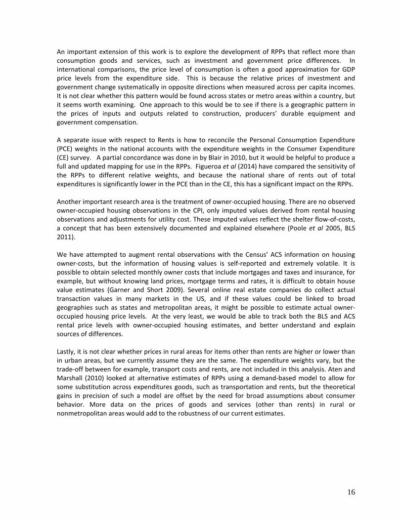
b) Regional Price Parities: States

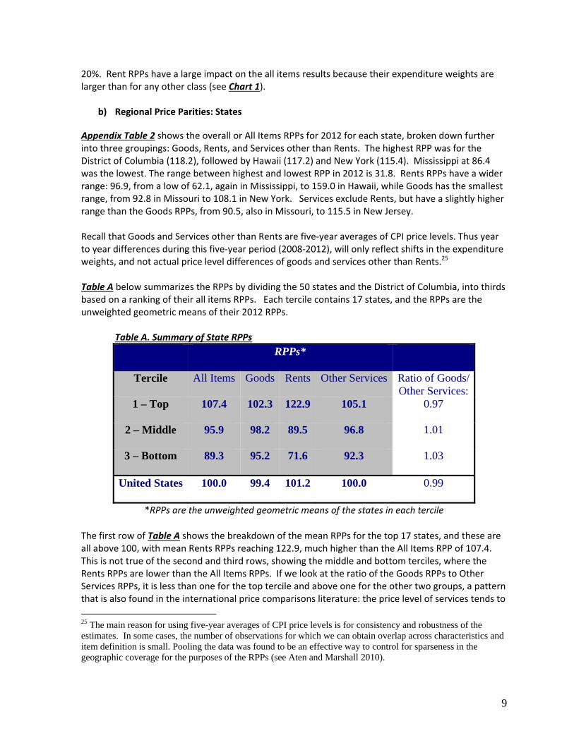
Appendix Table 2 shows the overall or All Items RPPs for 2012 for each state, broken down further into three groupings: Goods, Rents, and Services other than Rents. The highest RPP was for the District of Columbia (118.2), followed by Hawaii (117.2) and New York (115.4). Mississippi at 86.4 was the lowest. The range between highest and lowest RPP in 2012 is 31.8. Rents RPPs have a wider range: 96.9, from a low of 62.1, again in Mississippi, to 159.0 in Hawaii, while Goods has the smallest range, from 92.8 in Missouri to 108.1 in New York. Services exclude Rents, but have a slightly higher range than the Goods RPPs, from 90.5, also in Missouri, to 115.5 in New Jersey. Recall that Goods and Services other than Rents are five‐year averages of CPI price levels. Thus year to year differences during this five‐year period (2008‐2012), will only reflect shifts in the expenditure weights, and not actual price level differences of goods and services other than Rents.25 Table A below summarizes the RPPs by dividing the 50 states and the District of Columbia, into thirds based on a ranking of their all items RPPs. Each tercile contains 17 states, and the RPPs are the unweighted geometric means of their 2012 RPPs.

Table A. Summary of State RPPs

RPPs*

Tercile All Items Goods Rents Other Services Ratio of Goods/Other Services:

1 – Top 107.4 102.3 122.9 105.1 0.97

2 – Middle 95.9 98.2 89.5 96.8 1.01

3 – Bottom 89.3 95.2 71.6 92.3 1.03

United States 100.0 99.4 101.2 100.0 0.99

*RPPs are the unweighted geometric means of the states in each tercile

The first row of Table A shows the breakdown of the mean RPPs for the top 17 states, and these are all above 100, with mean Rents RPPs reaching 122.9, much higher than the All Items RPP of 107.4. This is not true of the second and third rows, showing the middle and bottom terciles, where the Rents RPPs are lower than the All Items RPPs. If we look at the ratio of the Goods RPPs to Other Services RPPs, it is less than one for the top tercile and above one for the other two groups, a pattern that is also found in the international price comparisons literature: the price level of services tends to

25 The main reason for using five-year averages of CPI price levels is for consistency and robustness of the estimates. In some cases, the number of observations for which we can obtain overlap across characteristics and item definition is small. Pooling the data was found to be an effective way to control for sparseness in the geographic coverage for the purposes of the RPPs (see Aten and Marshall 2010).

10

move in the same direction as that of rents, whereas goods will generally become relatively less expensive as the overall price level increases.

c) Per capita personal income: States

Appendix Table 3 shows the nominal and real per capita personal incomes and growth rates for

states. The pattern mimics the total personal incomes tables (Table 1) in that the range for real

incomes decreases and North Dakota is an outlier in both cases, with nominal per capita income

growth of 16.2% and real per capita income growth of 12.7%. South Dakota drops from 1.2% to ‐2.3%

in real terms, while the District of Columbia drops from 0.4% in nominal per capita terms to ‐1.7% in

real terms. The District saw one of the largest population increases in 2012, so that in spite of a small

positive growth in total real personal income, the per capita numbers show a decline in real income.

Table B highlights the highest and lowest per capita personal income states in 2011 and 2012. The

range in nominal per capita incomes for states is $41,116, between DC and Mississippi, and for real

per capita incomes it is $25,179 in 2008 dollars, between D.C. ($59,759) and Utah ($34,580).

Table B. Highest and Lowest per capita Personal Income: States 2012

Chart 3 shows the relationship between the RPPs and per capita personal incomes for 2012. The RPPs are plotted on the vertical axis against the nominal and real per capita personal incomes. The RPPs are in natural logs to more easily interpret the regression coefficients on the trend lines (the

RPP

2011 2012Percent

growth2011 2012

Percent

growth2012

Highest Per Capita

Personal Income

District of Columbia 74,480 74,773 0.4 60,787 59,759 ‐1.7 118.2

Connecticut 57,758 59,687 3.3 50,877 51,559 1.3 109.4

Massachusetts 54,218 55,976 3.2 48,320 49,354 2.1 107.2

New Jersey 53,333 54,987 3.1 45,021 45,552 1.2 114.1

North Dakota 47,218 54,871 16.2 50,923 57,367 12.7 90.4

Lowest Per Capita

Personal Income

Utah 34,173 35,430 3.7 33,963 34,580 1.8 96.8

West Virginia 33,822 35,082 3.7 36,784 37,425 1.7 88.6

South Carolina 34,183 35,056 2.6 36,291 36,507 0.6 90.7

Idaho 33,436 34,481 3.1 34,485 34,818 1.0 93.6

Mississippi 32,193 33,657 4.5 35,690 36,803 3.1 86.4

United States 42,298 43,735 3.4 40,663 41,282 1.5 100.0

Per Capita Personal Income

Dollars

Real Per Capita Personal

Income

Chained (2008) dollars

11

U.S. with an RPP = 100 is also plotted on the horizontal axis)26. For nominal incomes, a dollar increase in per capita incomes is associated with a 0.8% change in the RPPs, while for real incomes, the effect is smaller (0.4%) but still positive.

Chart 3. State RPPs and per capita personal income

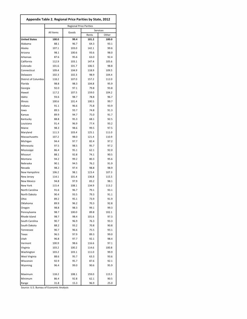
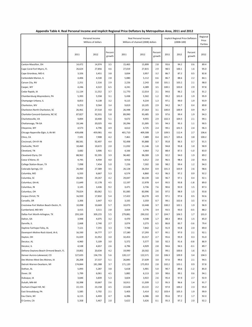
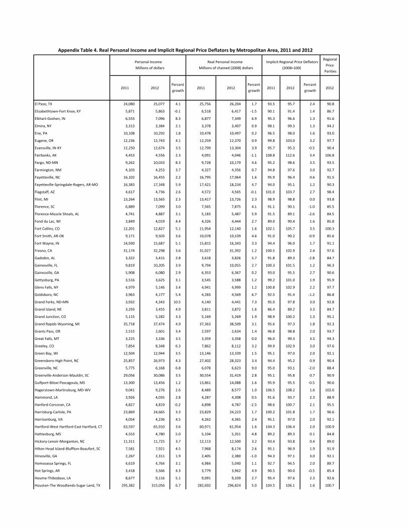
2) Metropolitan Statistical Areas (MSAs)

a) Total Personal Income and RPPs

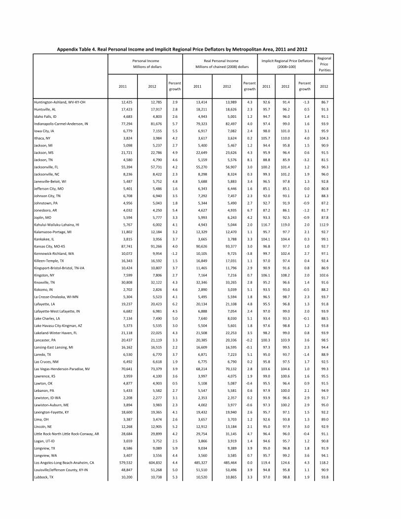
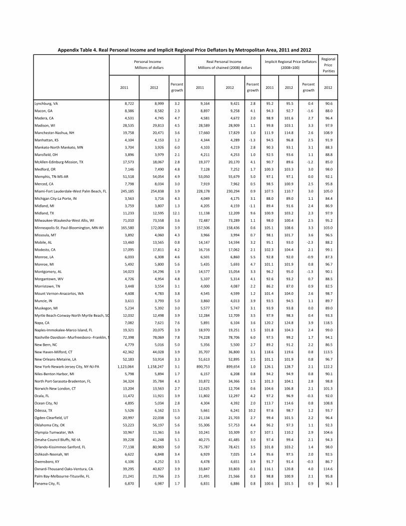
Appendix Table 4 lists all the metropolitan statistical areas (MSAs) and the non‐metropolitan portion of the U.S.. Similar to Appendix Table 1, it shows the nominal personal income totals in millions of dollars in the first columns, the real personal income totals in chained 2008 dollars in the next columns, the implicit price growth rates and the RPPs. The range of price growth is larger than across

26 The leftward shift along the horizontal axis is equal to the difference between U.S. nominal ($43,735)and real ($41,282) per capita totals for 2012, and reflects the 5.9% increase in the U.S. PCE price index between 2012 and 2008.

12

states, from ‐3.6% in Danville, IL, to 5.9% in State College, PA. However, the range of real income growth is less, from ‐3.8% in Kennewick‐Richland, WA, to 10.2% in Odessa, TX. Chart 4, like Chart 2, shows the relationship between the two growth rates, with personal income on the vertical and price growth on the horizontal axis. Chart 4. MSAs Total Real Personal Income and Implicit Price Growth 2012

As expected, metro areas in North Dakota such as Bismarck, Grand Forks and Fargo have both high income growth and high price growth, while Yuma, AZ shows a decline in prices (‐0.5%) and a decrease in its real personal income growth (‐1.1%). The MSAs in the upper right hand quadrant, shown in red, have above U.S. average income and price growth. The range of RPPs across MSAs is also higher than across states (43.5 versus 31.8), with Urban Honolulu, HI (122.9), New York‐Newark‐Jersey City, NY‐NJ‐PA (122.2) and San Jose‐Sunnyvale‐Santa Clara, CA (122.0) leading at the top, and Danville, IL (79.4), Jefferson City,MO (80.8) and Jackson, TN (81.5) at the lower end of the RPPs. The non‐metropolitan portion of the U.S. has an RPP of 87.9.

13

Table C is a summary of the MSA RPPs, divided into quintiles, with about 74 MSAs in each group ‐ there are a total of 366 MSAs, plus the non‐metro portion of the United States.

Table C. Summary of MSA RPPs

RPPs*

Quintile All Items Goods Rents Other Services Ratio of Goods/Other Services:

1 – Top 106.2 101.2 122.0 103.4 0.98

2 – Upper Middle 96.4 97.9 93.0 96.7 1.01

3 – Middle 93.2 97.2 82.1 95.0 1.02

4 – Lower Middle 90.8 96.9 74.4 94.0 1.03

5 – Bottom 86.5 95.4 64.1 92.6 1.03

United States 100.0 99.4 101.2 100.0 0.99

Similar to the state‐level results, the Rents RPP is higher than the All Items RPP for the top quintile (122.0 versus 106.2), but lower for the other quintiles. The ratio of the Goods RPP to the Other Services RPP is less than one for the top group but increases systematically to 1.03 for the bottom quintile as it did for the state terciles. That is, the price level of Goods tends to be higher than that of other services, and of rents, as the All Items RPPs decrease.

b) Per capita personal income: MSAs

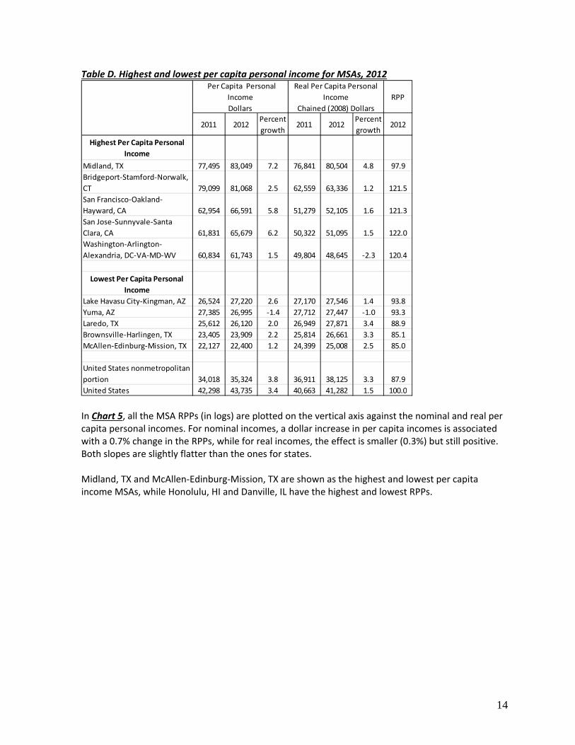
Appendix Table 5 lists the nominal and real per capita personal incomes and growth rates for the MSAs. The income growth ranges from a high of 9.5% in nominal values for Grand Forks, ND‐MN and 7.9% in real terms for Pine Bluff, AR, to a low of ‐2.8% and ‐5.4% in Kennewick‐Richland, WA in nominal and real terms respectively. Table D shows the five highest and lowest per capita income MSAs. The range is higher than for states: $60,649 in nominal terms and $55,495 in 2008 dollars, with Midland TX at $80,504 and McAllen‐Edinburg‐Mission, TX at $25,008. These two metropolitan areas in Texas also mark the extremes in nominal per capita income levels.

14

Table D. Highest and lowest per capita personal income for MSAs, 2012

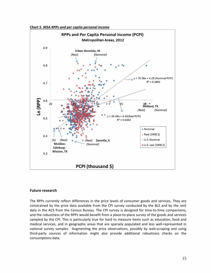
In Chart 5, all the MSA RPPs (in logs) are plotted on the vertical axis against the nominal and real per capita personal incomes. For nominal incomes, a dollar increase in per capita incomes is associated with a 0.7% change in the RPPs, while for real incomes, the effect is smaller (0.3%) but still positive. Both slopes are slightly flatter than the ones for states. Midland, TX and McAllen‐Edinburg‐Mission, TX are shown as the highest and lowest per capita income MSAs, while Honolulu, HI and Danville, IL have the highest and lowest RPPs.

RPP

2011 2012Percent

growth2011 2012

Percent

growth2012

Highest Per Capita Personal

Income

Midland, TX 77,495 83,049 7.2 76,841 80,504 4.8 97.9

Bridgeport‐Stamford‐Norwalk,

CT 79,099 81,068 2.5 62,559 63,336 1.2 121.5

San Francisco‐Oakland‐

Hayward, CA 62,954 66,591 5.8 51,279 52,105 1.6 121.3

San Jose‐Sunnyvale‐Santa

Clara, CA 61,831 65,679 6.2 50,322 51,095 1.5 122.0

Washington‐Arlington‐

Alexandria, DC‐VA‐MD‐WV 60,834 61,743 1.5 49,804 48,645 ‐2.3 120.4

Lowest Per Capita Personal

Income

Lake Havasu City‐Kingman, AZ 26,524 27,220 2.6 27,170 27,546 1.4 93.8

Yuma, AZ 27,385 26,995 ‐1.4 27,712 27,447 ‐1.0 93.3

Laredo, TX 25,612 26,120 2.0 26,949 27,871 3.4 88.9

Brownsville‐Harlingen, TX 23,405 23,909 2.2 25,814 26,661 3.3 85.1

McAllen‐Edinburg‐Mission, TX 22,127 22,400 1.2 24,399 25,008 2.5 85.0

United States nonmetropolitan

portion 34,018 35,324 3.8 36,911 38,125 3.3 87.9

United States 42,298 43,735 3.4 40,663 41,282 1.5 100.0

Per Capita Personal

Income

Dollars

Real Per Capita Personal

Income

Chained (2008) Dollars

15

Chart 5. MSA RPPs and per capita personal income

Future research

The RPPs currently reflect differences in the price levels of consumer goods and services. They are constrained by the price data available from the CPI survey conducted by the BLS and by the rent data in the ACS from the Census Bureau. The CPI survey is designed for time‐to‐time comparisons, and the robustness of the RPPs would benefit from a place‐to‐place survey of the goods and services sampled by the CPI. This is particularly true for hard to measure items such as education, food and medical services, and in geographic areas that are sparsely populated and less well‐represented in national survey samples. Augmenting the price observations, possibly by web‐scraping and using third‐party sources of information might also provide additional robustness checks on the consumptions data.

16

An important extension of this work is to explore the development of RPPs that reflect more than consumption goods and services, such as investment and government price differences. In international comparisons, the price level of consumption is often a good approximation for GDP price levels from the expenditure side. This is because the relative prices of investment and government change systematically in opposite directions when measured across per capita incomes. It is not clear whether this pattern would be found across states or metro areas within a country, but it seems worth examining. One approach to this would be to see if there is a geographic pattern in the prices of inputs and outputs related to construction, producers’ durable equipment and government compensation. A separate issue with respect to Rents is how to reconcile the Personal Consumption Expenditure (PCE) weights in the national accounts with the expenditure weights in the Consumer Expenditure (CE) survey. A partial concordance was done in by Blair in 2010, but it would be helpful to produce a full and updated mapping for use in the RPPs. Figueroa et al (2014) have compared the sensitivity of the RPPs to different relative weights, and because the national share of rents out of total expenditures is significantly lower in the PCE than in the CE, this has a significant impact on the RPPs. Another important research area is the treatment of owner‐occupied housing. There are no observed owner‐occupied housing observations in the CPI, only imputed values derived from rental housing observations and adjustments for utility cost. These imputed values reflect the shelter flow‐of‐costs, a concept that has been extensively documented and explained elsewhere (Poole et al 2005, BLS 2011). We have attempted to augment rental observations with the Census’ ACS information on housing owner‐costs, but the information of housing values is self‐reported and extremely volatile. It is possible to obtain selected monthly owner costs that include mortgages and taxes and insurance, for example, but without knowing land prices, mortgage terms and rates, it is difficult to obtain house value estimates (Garner and Short 2009). Several online real estate companies do collect actual transaction values in many markets in the US, and if these values could be linked to broad geographies such as states and metropolitan areas, it might be possible to estimate actual owner‐occupied housing price levels. At the very least, we would be able to track both the BLS and ACS rental price levels with owner‐occupied housing estimates, and better understand and explain sources of differences. Lastly, it is not clear whether prices in rural areas for items other than rents are higher or lower than in urban areas, but we currently assume they are the same. The expenditure weights vary, but the trade‐off between for example, transport costs and rents, are not included in this analysis. Aten and Marshall (2010) looked at alternative estimates of RPPs using a demand‐based model to allow for some substitution across expenditures goods, such as transportation and rents, but the theoretical gains in precision of such a model are offset by the need for broad assumptions about consumer behavior. More data on the prices of goods and services (other than rents) in rural or nonmetropolitan areas would add to the robustness of our current estimates.

17

Data Availability

Real personal income data, regional price parities, and implicit regional price deflators are available through the BEA website. Data are available for 2008 to 2012 for states, state metropolitan and nonmetropolitan portions, and metropolitan areas at www.bea.gov To access the data, select the “Interactive Data” tab at the top of the homepage. At the next screen, select “GDP & Personal Income” under Regional Data. Data are available in two formats through these links:

‐ Begin using the data: interactive tables where users specify data type, region and time period. ‐ Download complete data sets: flat files accessed through State or Local Area Personal Income menus.

For further information about these data, email the Regional Prices Branch at [email protected]

Acknowledgements The authors gratefully acknowledge the contribution of Troy M. Martin to the development and preparation of the RPPs. This work would not be possible without the collaboration of the Bureau of Labor Statistics and the Census Bureau. In particular, we thank the staff of the Consumer Price Index (CPI) program in the Office of Prices and Living Conditions at BLS and the staff of the Social, Economic and Housing Statistics Division of the Census Bureau for their technical and programmatic assistance.

18

References

Aten, Bettina (2005), ‘Report on Interarea Price Levels, 2003’, working paper 2005–11, Bureau of Economic Analysis, May. http://bea.gov/papers/working_papers.htm

Aten, Bettina (2006), ‘Interarea Price Levels: an experimental methodology’, Monthly Labor Review,

Vol. 129, No.9, Bureau of Labor Statistics, Washington, DC, September.

Aten, Bettina (2008), ‘Estimates of State and Metropolitan Price Parities for Consumption Goods and services in the United States, 2005’, Bureau of Economic Analysis, April. http://bea.gov/papers

Aten Bettina and Roger D’Souza (2008), ‘Regional Price Parities: Comparing Price Level Differences

Across Geographic Areas.’ Survey of Current Business, November. Aten, Bettina and Marshall Reinsdorf (2010), ‘Comparing the Consistency of Price Parities for Regions

of the U.S. in an Economic Approach Framework.’ 31st General Conference of the International Association for Research in Income and Wealth, August. http://www.bea.gov/papers.

Aten, Bettina, Eric Figueroa and Troy Martin (2011), ‘Notes on Estimating the Multi-Year Regional

Price Parities by 16 Expenditure Categories: 2005-2009’, Bureau of Economic Analysis, April. http://bea.gov/papers

Aten, Bettina H., Eric B. Figueroa, and Troy M. Martin (2012), “Regional Price Parities for States and

Metropolitan Areas, 2006–2010.” Survey of Current Business, 92 (August): 229–242. Aten, Bettina H., Eric B. Figueroa, and Troy M. Martin (2013), “Real Personal Income and Regional

Price Parities for States and Metropolitan Areas, 2007–2011.” Survey of Current Business, 93 (August): 89‐103.

Aten, Bettina H., and Eric B. Figueroa (2014), “Real Personal Income and Regional Price Parities for

State and Metropolitan Areas, 2008–2012.” Survey of Current Business, 94 (June): 1=8. Blair, Caitlin (2012), ‘Constructing a PCE‐Weighted Consumer Price Index.’ National Bureau of

Economic Research (NBER) Working Paper (March); www.nber.org. BLS Handbook of Methods (2011), Bureau of Labor Statistics.

http://www.bls.gov/opub/hom/homtoc.htm Deaton, Angus and Alan Heston (2010), ‘Understanding PPPs and PPP‐Based National Accounts’,

American Economic Journal: Macroeconomics 2, no.4 (October): 1‐35. Figueroa, Eric, Bettina Aten and Troy Martin (2014), ‘Expenditure Weights in the Regional Price

Parities’, Bureau of Economic Analysis, May. http://bea.gov/papers Garner, Thesia and Kathleen Short (2009), ‘Accounting for Owner‐occupied dwelling services:

aggregates and distributions’, Journal of Housing Economics, 18 233‐248.

19

Martin, Troy, Bettina Aten and Eric Figueroa (2011), ‘Estimating the Price of Rents in Regional Price

Parities’, Bureau of Economic Analysis, October. http://bea.gov/papers Poole, Robert, Frank Ptacek and Randal Verbrugge (2005), ‘Treatment of Owner‐Occupied Housing in

the CPI,’ Bureau of Labor Statistics. http://www.bls.gov/bls/fesacp1120905.pdf Rao, D.S. Prasada (2004), ‘On the Equivalence of Weighted Country‐Product‐Dummy (CPD) Method

and the Rao System for Multilateral Price Comparisons’, Review of Income and Wealth, 51, 571‐580.

2011 2012Percent

growth2011 2012

Percent

growth2011 2012

Percent

growth

United States 13,179,561 13,729,063 4.2 12,670,133 12,958,961 2.3 104.0 105.9 1.8

Alabama 167,787 173,236 3.2 184,281 185,792 0.8 91.0 93.2 2.4

Alaska 34,827 36,160 3.8 31,686 31,892 0.7 109.9 113.4 3.2

Arizona 229,238 237,513 3.6 224,381 228,740 1.9 102.2 103.8 1.6

Arkansas 100,005 104,508 4.5 109,913 112,726 2.6 91.0 92.7 1.9

California 1,683,204 1,768,039 5.0 1,430,212 1,479,356 3.4 117.7 119.5 1.6

Colorado 226,032 237,461 5.1 214,906 220,778 2.7 105.2 107.6 2.3

Connecticut 207,162 214,297 3.4 182,483 185,116 1.4 113.5 115.8 2.0

Delaware 38,873 40,558 4.3 36,575 37,461 2.4 106.3 108.3 1.9

District of Columbia 46,104 47,281 2.6 37,628 37,787 0.4 122.5 125.1 2.1

Florida 761,303 792,255 4.1 739,169 757,737 2.5 103.0 104.6 1.5

Georgia 356,836 371,488 4.1 373,328 381,708 2.2 95.6 97.3 1.8

Hawaii 60,095 62,330 3.7 49,551 50,245 1.4 121.3 124.1 2.3

Idaho 52,954 55,022 3.9 54,616 55,561 1.7 97.0 99.0 2.1

Illinois 567,197 590,094 4.0 541,432 554,445 2.4 104.8 106.4 1.6

Indiana 236,815 249,198 5.2 249,422 258,572 3.7 94.9 96.4 1.5

Iowa 130,131 135,063 3.8 139,994 142,567 1.8 93.0 94.7 1.9

Kansas 120,783 124,137 2.8 129,263 130,490 0.9 93.4 95.1 1.8

Kentucky 150,850 156,131 3.5 163,899 166,058 1.3 92.0 94.0 2.2

Louisiana 176,690 184,340 4.3 186,955 190,667 2.0 94.5 96.7 2.3

Maine 51,653 53,283 3.2 51,018 51,195 0.3 101.2 104.1 2.8

Maryland 306,001 316,682 3.5 264,482 268,936 1.7 115.7 117.8 1.8

Massachusetts 358,218 372,026 3.9 319,250 328,017 2.7 112.2 113.4 1.1

Michigan 365,753 378,443 3.5 372,860 378,704 1.6 98.1 99.9 1.9

Minnesota 241,352 252,413 4.6 239,548 244,719 2.2 100.8 103.1 2.4

Mississippi 95,854 100,465 4.8 106,266 109,854 3.4 90.2 91.5 1.4

Missouri 228,270 235,661 3.2 248,780 252,687 1.6 91.8 93.3 1.6

Montana 36,630 38,753 5.8 37,479 38,864 3.7 97.7 99.7 2.0

Nebraska 80,420 83,521 3.9 86,224 87,558 1.5 93.3 95.4 2.3

Nevada 101,717 105,450 3.7 98,566 101,444 2.9 103.2 103.9 0.7

New Hampshire 62,651 64,885 3.6 57,116 57,745 1.1 109.7 112.4 2.4

New Jersey 471,188 487,437 3.4 397,749 403,804 1.5 118.5 120.7 1.9

New Mexico 72,300 74,416 2.9 73,263 74,147 1.2 98.7 100.4 1.7

New York 1,012,406 1,041,931 2.9 844,330 853,317 1.1 119.9 122.1 1.8

North Carolina 352,455 369,704 4.9 371,148 381,336 2.7 95.0 96.9 2.1

North Dakota 32,332 38,390 18.7 34,869 40,136 15.1 92.7 95.6 3.2

Ohio 446,136 462,424 3.7 480,076 489,788 2.0 92.9 94.4 1.6

Oklahoma 147,430 154,958 5.1 158,458 162,898 2.8 93.0 95.1 2.2

Oregon 146,001 152,722 4.6 142,547 146,033 2.4 102.4 104.6 2.1

Pennsylvania 558,345 575,425 3.1 545,333 551,039 1.0 102.4 104.4 2.0

Rhode Island 46,881 48,184 2.8 45,372 46,113 1.6 103.3 104.5 1.1

South Carolina 159,747 165,595 3.7 169,599 172,448 1.7 94.2 96.0 1.9

South Dakota 36,932 37,819 2.4 40,997 40,523 ‐1.2 90.1 93.3 3.6

Tennessee 237,618 250,189 5.3 253,494 260,645 2.8 93.7 96.0 2.4

Texas 1,053,552 1,111,110 5.5 1,053,124 1,087,533 3.3 100.0 102.2 2.1

Utah 96,175 101,163 5.2 95,583 98,737 3.3 100.6 102.5 1.8

Vermont 26,888 27,886 3.7 25,863 26,121 1.0 104.0 106.8 2.7

Virginia 381,930 396,005 3.7 356,882 362,744 1.6 107.0 109.2 2.0

Washington 303,088 317,575 4.8 283,739 290,802 2.5 106.8 109.2 2.2

West Virginia 62,737 65,091 3.8 68,230 69,438 1.8 91.9 93.7 1.9

Wisconsin 232,094 241,201 3.9 240,443 245,355 2.0 96.5 98.3 1.8

Wyoming 27,920 29,147 4.4 27,749 28,583 3.0 100.6 102.0 1.3

Maximum 1,683,204 1,768,039 18.7 1,430,212 1,479,356 15.1 122.5 125.1 3.6

Minimum 26,888 27,886 2.4 25,863 26,121 ‐1.2 90.1 91.5 0.7

Range 1,656,316 1,740,153 16.3 1,404,348 1,453,234 16.3 32.4 33.7 2.9

Source: U.S. Bureau of Economic Analysis

Appendix Table 1. Real Personal Income and Implicit Regional Price Deflators by State, 2011 and 2012

Personal Income

Millions of dollars

Real Personal Income

Millions of chained (2008) dollars

Implicit Regional Price Deflators

(2008=100)

Rents Other

United States 100.0 99.4 101.2 100.0

Alabama 88.1 96.7 64.3 93.1

Alaska 107.1 103.0 142.1 99.6

Arizona 98.1 100.6 93.6 98.0

Arkansas 87.6 95.6 63.0 92.4

California 112.9 103.1 147.4 105.6

Colorado 101.6 101.7 106.5 98.8

Connecticut 109.4 104.9 118.9 109.5

Delaware 102.3 102.3 98.9 104.4

District of Columbia 118.2 107.0 157.2 112.0

Florida 98.8 98.3 104.8 95.9

Georgia 92.0 97.1 79.8 93.8

Hawaii 117.2 107.5 159.0 104.2

Idaho 93.6 98.7 78.8 96.7

Illinois 100.6 101.4 100.5 99.7

Indiana 91.1 96.6 75.8 93.9

Iowa 89.5 93.7 74.8 91.3

Kansas 89.9 94.7 75.0 91.7

Kentucky 88.8 95.3 68.1 92.5

Louisiana 91.4 96.9 77.4 93.2

Maine 98.3 98.6 99.5 97.5

Maryland 111.3 103.4 125.1 111.0

Massachusetts 107.2 98.0 121.4 110.9

Michigan 94.4 97.7 82.4 97.2

Minnesota 97.5 98.5 95.7 97.2

Mississippi 86.4 95.1 62.1 92.0

Missouri 88.1 92.8 74.1 90.5

Montana 94.2 99.2 80.3 95.6

Nebraska 90.1 94.5 76.2 91.9

Nevada 98.2 97.4 98.8 98.9

New Hampshire 106.2 98.1 123.4 107.3

New Jersey 114.1 101.4 136.8 115.5

New Mexico 94.8 97.9 83.2 98.1

New York 115.4 108.1 134.9 113.2

North Carolina 91.6 96.7 79.1 93.1

North Dakota 90.4 93.5 79.3 91.1

Ohio 89.2 95.1 73.9 91.9

Oklahoma 89.9 96.2 70.3 92.8

Oregon 98.8 98.3 99.1 99.3

Pennsylvania 98.7 100.0 89.8 102.1

Rhode Island 98.7 98.4 101.6 97.3

South Carolina 90.7 96.9 76.3 93.3

South Dakota 88.2 93.2 70.8 90.8

Tennessee 90.7 96.6 75.5 93.1

Texas 96.5 97.9 89.3 99.0

Utah 96.8 97.7 92.1 98.4

Vermont 100.9 98.6 116.6 97.1

Virginia 103.2 100.2 114.6 100.8

Washington 103.2 103.1 111.0 99.9

West Virginia 88.6 95.7 63.3 93.6

Wisconsin 92.9 95.7 87.6 92.1

Wyoming 96.4 99.0 90.6 95.9

Maximum 118.2 108.1 159.0 115.5

Minimum 86.4 92.8 62.1 90.5

Range 31.8 15.3 96.9 25.0


Appendix Table 2. Regional Price Parities by State, 2012

Regional Price Parities

All Items GoodsServices

2011 2012Percent

growth2011 2012

Percent

growth

United States 42,298 43,735 3.4 40,663 41,282 1.5

Alabama 34,929 35,926 2.9 38,362 38,530 0.4

Alaska 48,114 49,436 2.7 43,773 43,601 ‐0.4

Arizona 35,446 36,243 2.3 34,695 34,905 0.6

Arkansas 34,032 35,437 4.1 37,403 38,223 2.2

California 44,666 46,477 4.1 37,953 38,888 2.5

Colorado 44,179 45,775 3.6 42,004 42,559 1.3

Connecticut 57,758 59,687 3.3 50,877 51,559 1.3

Delaware 42,805 44,224 3.3 40,275 40,848 1.4

District of Columbi 74,480 74,773 0.4 60,787 59,759 ‐1.7

Florida 39,896 41,012 2.8 38,736 39,225 1.3

Georgia 36,366 37,449 3.0 38,046 38,479 1.1

Hawaii 43,606 44,767 2.7 35,955 36,087 0.4

Idaho 33,436 34,481 3.1 34,485 34,818 1.0

Illinois 44,106 45,832 3.9 42,103 43,063 2.3

Indiana 36,342 38,119 4.9 38,276 39,553 3.3

Iowa 42,470 43,935 3.4 45,688 46,376 1.5

Kansas 42,079 43,015 2.2 45,033 45,216 0.4

Kentucky 34,545 35,643 3.2 37,533 37,909 1.0

Louisiana 38,623 40,057 3.7 40,867 41,432 1.4

Maine 38,880 40,087 3.1 38,402 38,516 0.3

Maryland 52,401 53,816 2.7 45,291 45,702 0.9

Massachusetts 54,218 55,976 3.2 48,320 49,354 2.1

Michigan 37,032 38,291 3.4 37,751 38,317 1.5

Minnesota 45,135 46,925 4.0 44,798 45,494 1.6

Mississippi 32,193 33,657 4.5 35,690 36,803 3.1

Missouri 37,988 39,133 3.0 41,401 41,961 1.4

Montana 36,716 38,555 5.0 37,566 38,665 2.9

Nebraska 43,654 45,012 3.1 46,804 47,188 0.8

Nevada 37,396 38,221 2.2 36,237 36,769 1.5

New Hampshire 47,542 49,129 3.3 43,342 43,722 0.9

New Jersey 53,333 54,987 3.1 45,021 45,552 1.2

New Mexico 34,782 35,682 2.6 35,245 35,553 0.9

New York 51,914 53,241 2.6 43,295 43,603 0.7

North Carolina 36,520 37,910 3.8 38,457 39,103 1.7

North Dakota 47,218 54,871 16.2 50,923 57,367 12.7

Ohio 38,657 40,057 3.6 41,597 42,427 2.0

Oklahoma 38,960 40,620 4.3 41,874 42,701 2.0

Oregon 37,744 39,166 3.8 36,851 37,451 1.6

Pennsylvania 43,813 45,083 2.9 42,792 43,173 0.9

Rhode Island 44,621 45,877 2.8 43,185 43,905 1.7

South Carolina 34,183 35,056 2.6 36,291 36,507 0.6

South Dakota 44,843 45,381 1.2 49,779 48,626 ‐2.3

Tennessee 37,129 38,752 4.4 39,610 40,371 1.9

Texas 41,103 42,638 3.7 41,087 41,733 1.6

Utah 34,173 35,430 3.7 33,963 34,580 1.8

Vermont 42,911 44,545 3.8 41,276 41,726 1.1

Virginia 47,126 48,377 2.7 44,036 44,313 0.6

Washington 44,420 46,045 3.7 41,584 42,164 1.4

West Virginia 33,822 35,082 3.7 36,784 37,425 1.7

Wisconsin 40,648 42,121 3.6 42,110 42,846 1.7

Wyoming 49,212 50,567 2.8 48,909 49,587 1.4

Maximum 74,480 74,773 16.2 60,787 59,759 12.7

Minimum 32,193 33,657 0.4 33,963 34,580 ‐2.3

Range 42,287 41,116 15.8 26,824 25,179 15.0


Appendix Table 3. Real Per Capita Personal Income by State, 2011 and 2012


Dollars

Real Per Capita Personal Income

Chained (2008) dollars

Regional

Price

Parities

2011 2012Percent

growth2011 2012

Percent

growth2011 2012

Percent

growth2012

Abilene, TX 6,070 6,331 4.3 6,360 6,575 3.4 95.4 96.3 0.9 91.4

Akron, OH 28,363 29,482 3.9 30,733 31,650 3.0 92.3 93.2 0.9 88.4

Albany, GA 5,147 5,345 3.8 5,557 5,958 7.2 92.6 89.7 ‐3.1 85.1

Albany, OR 3,530 3,667 3.9 3,646 3,714 1.9 96.8 98.8 2.0 93.7

Albany‐Schenectady‐Troy, NY 40,684 41,776 2.7 39,636 39,992 0.9 102.6 104.5 1.8 99.1

Albuquerque, NM 31,881 32,707 2.6 32,078 32,143 0.2 99.4 101.8 2.4 96.6

Alexandria, LA 5,554 5,783 4.1 5,940 6,258 5.4 93.5 92.4 ‐1.2 87.7

Allentown‐Bethlehem‐Easton, PA‐NJ 34,225 35,457 3.6 32,996 33,665 2.0 103.7 105.3 1.5 99.9

Altoona, PA 4,562 4,649 1.9 4,804 4,826 0.5 95.0 96.3 1.5 91.4

Amarillo, TX 9,583 9,876 3.1 9,969 10,095 1.3 96.1 97.8 1.8 92.8

Ames, IA 3,826 4,062 6.2 4,220 4,347 3.0 90.7 93.4 3.0 88.7

Anchorage, AK 19,711 20,553 4.3 17,454 17,590 0.8 112.9 116.8 3.5 110.9

Ann Arbor, MI 14,380 15,162 5.4 13,709 14,083 2.7 104.9 107.7 2.6 102.2

Anniston‐Oxford‐Jacksonville, AL 3,817 3,857 1.0 4,179 4,314 3.2 91.3 89.4 ‐2.1 84.8

Appleton, WI 9,110 9,549 4.8 9,445 9,707 2.8 96.5 98.4 2.0 93.3

Asheville, NC 14,906 15,621 4.8 15,667 16,117 2.9 95.1 96.9 1.9 92.0

Athens‐Clarke County, GA 6,228 6,496 4.3 6,527 6,711 2.8 95.4 96.8 1.4 91.8

Atlanta‐Sandy Springs‐Roswell, GA 214,363 223,569 4.3 214,235 221,843 3.6 100.1 100.8 0.7 95.6

Atlantic City‐Hammonton, NJ 11,319 11,595 2.4 10,014 10,150 1.4 113.0 114.2 1.1 108.4

Auburn‐Opelika, AL 4,258 4,452 4.6 4,639 4,858 4.7 91.8 91.6 ‐0.2 87.0

Augusta‐Richmond County, GA‐SC 20,134 20,703 2.8 21,192 21,876 3.2 95.0 94.6 ‐0.4 89.8

Austin‐Round Rock, TX 74,169 78,696 6.1 72,970 75,828 3.9 101.6 103.8 2.1 98.5

Bakersfield, CA 27,836 29,497 6.0 27,834 28,764 3.3 100.0 102.5 2.5 97.3

Baltimore‐Columbia‐Towson, MD 143,281 149,222 4.1 125,880 129,483 2.9 113.8 115.2 1.2 109.4

Bangor, ME 5,355 5,513 3.0 5,411 5,391 ‐0.4 99.0 102.3 3.3 97.0

Barnstable Town, MA 12,475 12,977 4.0 11,861 12,063 1.7 105.2 107.6 2.3 102.1

Baton Rouge, LA 31,228 32,811 5.1 32,213 33,414 3.7 96.9 98.2 1.3 93.2

Battle Creek, MI 4,644 4,813 3.6 4,911 5,044 2.7 94.6 95.4 0.9 90.5

Bay City, MI 3,660 3,717 1.5 3,892 3,969 2.0 94.0 93.6 ‐0.4 88.9

Beaumont‐Port Arthur, TX 14,936 15,510 3.8 15,702 16,248 3.5 95.1 95.5 0.4 90.6

Beckley, WV 4,292 4,420 3.0 4,868 4,887 0.4 88.2 90.4 2.6 85.8

Bellingham, WA 7,721 8,029 4.0 7,594 7,675 1.1 101.7 104.6 2.9 99.3

Bend‐Redmond, OR 5,965 6,239 4.6 6,078 6,127 0.8 98.1 101.8 3.8 96.6

Billings, MT 6,423 6,766 5.3 6,569 6,723 2.3 97.8 100.6 2.9 95.5

Binghamton, NY 9,334 9,535 2.2 9,555 9,464 ‐1.0 97.7 100.8 3.1 95.6

Birmingham‐Hoover, AL 45,623 47,569 4.3 47,235 50,056 6.0 96.6 95.0 ‐1.6 90.2

Bismarck, ND 5,043 5,554 10.1 5,328 5,607 5.2 94.7 99.1 4.6 94.0

Blacksburg‐Christiansburg‐Radford, VA 5,363 5,629 5.0 5,767 6,016 4.3 93.0 93.6 0.6 88.8

Bloomington, IL 7,950 8,196 3.1 8,131 8,224 1.1 97.8 99.7 1.9 94.6

Bloomington, IN 5,104 5,333 4.5 5,310 5,420 2.1 96.1 98.4 2.4 93.4

Bloomsburg‐Berwick, PA 2,961 3,059 3.3 3,111 3,157 1.5 95.2 96.9 1.8 92.0

Boise City, ID 21,677 22,552 4.0 22,296 22,604 1.4 97.2 99.8 2.6 94.7

Boston‐Cambridge‐Newton, MA‐NH 269,576 280,244 4.0 235,321 238,363 1.3 114.6 117.6 2.6 111.6

Boulder, CO 15,487 16,418 6.0 14,081 14,300 1.6 110.0 114.8 4.4 108.9

Bowling Green, KY 5,032 5,221 3.8 5,694 5,822 2.2 88.4 89.7 1.5 85.1

Bremerton‐Silverdale, WA 10,975 11,359 3.5 10,214 10,301 0.8 107.4 110.3 2.6 104.6

Bridgeport‐Stamford‐Norwalk, CT 73,370 75,704 3.2 58,028 59,145 1.9 126.4 128.0 1.2 121.5

Brownsville‐Harlingen, TX 9,656 9,936 2.9 10,650 11,079 4.0 90.7 89.7 ‐1.1 85.1

Brunswick, GA 3,781 3,911 3.4 4,201 4,311 2.6 90.0 90.7 0.8 86.1

Buffalo‐Cheektowaga‐Niagara Falls, NY 47,125 48,530 3.0 48,037 49,080 2.2 98.1 98.9 0.8 93.8

Burlington, NC 4,848 5,068 4.5 5,119 5,346 4.4 94.7 94.8 0.1 90.0

Burlington‐South Burlington, VT 9,691 10,105 4.3 9,205 9,376 1.9 105.3 107.8 2.4 102.3

California‐Lexington Park, MD 5,061 5,189 2.5 4,800 4,814 0.3 105.4 107.8 2.2 102.3

Personal Income

Millions of dollars




(2008=100)

Appendix Table 4. Real Personal Income and Implicit Regional Price Deflators by Metropolitan Area, 2011 and 2012

Regional

Price

Parities

2011 2012Percent

growth2011 2012

Percent

growth2011 2012

Percent

growth2012

Personal Income

Millions of dollars




(2008=100)


Canton‐Massillon, OH 14,472 14,974 3.5 15,465 15,899 2.8 93.6 94.2 0.6 89.4

Cape Coral‐Fort Myers, FL 26,624 27,856 4.6 27,019 27,815 2.9 98.5 100.1 1.6 95.0

Cape Girardeau, MO‐IL 3,326 3,451 3.8 3,834 3,957 3.2 86.7 87.2 0.5 82.8

Carbondale‐Marion, IL 4,406 4,530 2.8 5,080 5,112 0.6 86.7 88.6 2.2 84.1

Carson City, NV 2,251 2,316 2.9 2,226 2,243 0.8 101.1 103.2 2.1 98.0

Casper, WY 4,246 4,522 6.5 4,241 4,389 3.5 100.1 103.0 2.9 97.8

Cedar Rapids, IA 11,134 11,552 3.7 11,770 12,014 2.1 94.6 96.2 1.6 91.2

Chambersburg‐Waynesboro, PA 5,393 5,558 3.1 5,438 5,502 1.2 99.2 101.0 1.9 95.9

Champaign‐Urbana, IL 8,853 9,138 3.2 9,115 9,234 1.3 97.1 99.0 1.9 93.9

Charleston, WV 9,253 9,564 3.4 9,819 10,105 2.9 94.2 94.7 0.4 89.8

Charleston‐North Charleston, SC 26,461 27,510 4.0 26,448 27,263 3.1 100.0 100.9 0.9 95.7

Charlotte‐Concord‐Gastonia, NC‐SC 87,827 92,931 5.8 89,990 93,485 3.9 97.6 99.4 1.9 94.3

Charlottesville, VA 9,894 10,400 5.1 9,672 9,955 2.9 102.3 104.5 2.1 99.1

Chattanooga, TN‐GA 19,146 20,025 4.6 20,296 21,005 3.5 94.3 95.3 1.1 90.5

Cheyenne, WY 4,573 4,796 4.9 4,612 4,725 2.4 99.1 101.5 2.4 96.3

Chicago‐Naperville‐Elgin, IL‐IN‐WI 439,698 459,981 4.6 401,710 409,308 1.9 109.5 112.4 2.7 106.6

Chico, CA 7,591 7,908 4.2 7,461 7,489 0.4 101.7 105.6 3.8 100.2

Cincinnati, OH‐KY‐IN 88,581 92,497 4.4 92,498 95,888 3.7 95.8 96.5 0.7 91.5

Clarksville, TN‐KY 10,460 10,672 2.0 11,032 11,146 1.0 94.8 95.8 1.0 90.9

Cleveland, TN 3,682 3,906 6.1 4,166 4,464 7.2 88.4 87.5 ‐1.0 83.0

Cleveland‐Elyria, OH 88,962 92,395 3.9 96,482 98,289 1.9 92.2 94.0 1.9 89.2

Coeur d'Alene, ID 4,745 4,934 4.0 4,916 5,012 2.0 96.5 98.4 2.0 93.4

College Station‐Bryan, TX 7,098 7,454 5.0 7,226 7,502 3.8 98.2 99.4 1.2 94.3

Colorado Springs, CO 26,460 27,389 3.5 26,128 26,354 0.9 101.3 103.9 2.6 98.6

Columbia, MO 6,333 6,667 5.3 6,574 6,860 4.3 96.3 97.2 0.9 92.2

Columbia, SC 28,091 29,267 4.2 29,047 30,139 3.8 96.7 97.1 0.4 92.1

Columbus, GA‐AL 11,649 12,178 4.5 12,197 12,978 6.4 95.5 93.8 ‐1.8 89.0

Columbus, IN 3,145 3,436 9.2 3,471 3,736 7.6 90.6 92.0 1.5 87.3

Columbus, OH 79,024 83,062 5.1 81,085 83,996 3.6 97.5 98.9 1.5 93.8

Corpus Christi, TX 16,920 17,832 5.4 17,422 18,270 4.9 97.1 97.6 0.5 92.6

Corvallis, OR 3,306 3,447 4.3 3,335 3,359 0.7 99.1 102.6 3.5 97.4

Crestview‐Fort Walton Beach‐Destin, FL 10,098 10,669 5.7 10,073 10,448 3.7 100.2 102.1 1.9 96.9

Cumberland, MD‐WV 3,415 3,511 2.8 3,654 3,776 3.4 93.5 93.0 ‐0.5 88.2

Dallas‐Fort Worth‐Arlington, TX 293,169 309,155 5.5 279,881 290,332 3.7 104.7 106.5 1.7 101.0

Dalton, GA 3,948 4,075 3.2 4,470 4,548 1.7 88.3 89.6 1.5 85.0

Danville, IL 2,668 2,740 2.7 3,074 3,273 6.5 86.8 83.7 ‐3.6 79.4

Daphne‐Fairhope‐Foley, AL 7,121 7,355 3.3 7,748 7,842 1.2 91.9 93.8 2.0 89.0

Davenport‐Moline‐Rock Island, IA‐IL 16,330 16,777 2.7 17,180 17,293 0.7 95.1 97.0 2.1 92.1

Dayton, OH 31,029 31,952 3.0 32,453 33,317 2.7 95.6 95.9 0.3 91.0

Decatur, AL 4,960 5,109 3.0 5,372 5,577 3.8 92.3 91.6 ‐0.8 86.9

Decatur, IL 4,538 4,657 2.6 4,796 4,929 2.8 94.6 94.5 ‐0.1 89.7

Deltona‐Daytona Beach‐Ormond Beach, FL 19,802 20,634 4.2 19,990 20,502 2.6 99.1 100.6 1.6 95.5

Denver‐Aurora‐Lakewood, CO 127,635 134,735 5.6 120,117 122,571 2.0 106.3 109.9 3.4 104.3

Des Moines‐West Des Moines, IA 26,208 27,537 5.1 26,845 27,639 3.0 97.6 99.6 2.1 94.5

Detroit‐Warren‐Dearborn, MI 174,844 181,388 3.7 171,120 175,953 2.8 102.2 103.1 0.9 97.8

Dothan, AL 5,093 5,287 3.8 5,618 5,901 5.0 90.7 89.6 ‐1.2 85.0

Dover, DE 5,799 6,061 4.5 5,882 6,113 3.9 98.6 99.1 0.6 94.1

Dubuque, IA 3,646 3,839 5.3 3,824 3,922 2.6 95.4 97.9 2.7 92.9

Duluth, MN‐WI 10,398 10,667 2.6 10,911 11,039 1.2 95.3 96.6 1.4 91.7

Durham‐Chapel Hill, NC 22,155 23,158 4.5 22,628 23,122 2.2 97.9 100.2 2.3 95.0

East Stroudsburg, PA 5,585 5,702 2.1 5,403 5,414 0.2 103.4 105.3 1.9 99.9

Eau Claire, WI 6,115 6,403 4.7 6,396 6,586 3.0 95.6 97.2 1.7 92.3

El Centro, CA 5,358 5,467 2.0 5,622 5,626 0.1 95.3 97.2 2.0 92.2

Regional

Price

Parities

2011 2012Percent

growth2011 2012

Percent

growth2011 2012

Percent

growth2012

Personal Income

Millions of dollars




(2008=100)


El Paso, TX 24,080 25,077 4.1 25,756 26,204 1.7 93.5 95.7 2.4 90.8

Elizabethtown‐Fort Knox, KY 5,871 5,863 ‐0.1 6,518 6,417 ‐1.5 90.1 91.4 1.4 86.7

Elkhart‐Goshen, IN 6,555 7,096 8.3 6,877 7,349 6.9 95.3 96.6 1.3 91.6

Elmira, NY 3,313 3,384 2.1 3,378 3,407 0.9 98.1 99.3 1.3 94.2

Erie, PA 10,108 10,292 1.8 10,478 10,497 0.2 96.5 98.0 1.6 93.0

Eugene, OR 12,236 12,743 4.1 12,259 12,370 0.9 99.8 103.0 3.2 97.7

Evansville, IN‐KY 12,250 12,674 3.5 12,799 13,304 3.9 95.7 95.3 ‐0.5 90.4

Fairbanks, AK 4,453 4,556 2.3 4,091 4,046 ‐1.1 108.8 112.6 3.4 106.8

Fargo, ND‐MN 9,262 10,033 8.3 9,728 10,179 4.6 95.2 98.6 3.5 93.5

Farmington, NM 4,103 4,253 3.7 4,327 4,356 0.7 94.8 97.6 3.0 92.7

Fayetteville, NC 16,102 16,455 2.2 16,795 17,064 1.6 95.9 96.4 0.6 91.5

Fayetteville‐Springdale‐Rogers, AR‐MO 16,383 17,348 5.9 17,421 18,234 4.7 94.0 95.1 1.2 90.3

Flagstaff, AZ 4,617 4,736 2.6 4,572 4,565 ‐0.1 101.0 103.7 2.7 98.4

Flint, MI 13,264 13,565 2.3 13,417 13,726 2.3 98.9 98.8 0.0 93.8

Florence, SC 6,889 7,099 3.0 7,565 7,875 4.1 91.1 90.1 ‐1.0 85.5

Florence‐Muscle Shoals, AL 4,741 4,887 3.1 5,183 5,487 5.9 91.5 89.1 ‐2.6 84.5

Fond du Lac, WI 3,849 4,019 4.4 4,326 4,444 2.7 89.0 90.4 1.6 85.8

Fort Collins, CO 12,201 12,827 5.1 11,954 12,140 1.6 102.1 105.7 3.5 100.3

Fort Smith, AR‐OK 9,171 9,503 3.6 10,078 10,539 4.6 91.0 90.2 ‐0.9 85.6

Fort Wayne, IN 14,930 15,687 5.1 15,815 16,343 3.3 94.4 96.0 1.7 91.1

Fresno, CA 31,174 32,298 3.6 31,027 31,392 1.2 100.5 102.9 2.4 97.6

Gadsden, AL 3,322 3,415 2.8 3,618 3,826 5.7 91.8 89.3 ‐2.8 84.7

Gainesville, FL 9,819 10,205 3.9 9,794 10,055 2.7 100.3 101.5 1.2 96.3

Gainesville, GA 5,908 6,080 2.9 6,353 6,367 0.2 93.0 95.5 2.7 90.6

Gettysburg, PA 3,516 3,625 3.1 3,545 3,588 1.2 99.2 101.0 1.9 95.9

Glens Falls, NY 4,979 5,146 3.4 4,941 4,999 1.2 100.8 102.9 2.2 97.7

Goldsboro, NC 3,963 4,177 5.4 4,283 4,569 6.7 92.5 91.4 ‐1.2 86.8

Grand Forks, ND‐MN 3,932 4,343 10.5 4,140 4,441 7.3 95.0 97.8 3.0 92.8

Grand Island, NE 3,293 3,455 4.9 3,811 3,872 1.6 86.4 89.2 3.3 84.7

Grand Junction, CO 5,115 5,282 3.3 5,169 5,269 1.9 98.9 100.2 1.3 95.1

Grand Rapids‐Wyoming, MI 35,718 37,474 4.9 37,363 38,509 3.1 95.6 97.3 1.8 92.3

Grants Pass, OR 2,515 2,601 3.4 2,597 2,634 1.4 96.8 98.8 2.0 93.7

Great Falls, MT 3,225 3,336 3.5 3,359 3,358 0.0 96.0 99.3 3.5 94.3

Greeley, CO 7,854 8,348 6.3 7,862 8,112 3.2 99.9 102.9 3.0 97.6

Green Bay, WI 12,504 12,944 3.5 13,146 13,339 1.5 95.1 97.0 2.0 92.1

Greensboro‐High Point, NC 25,857 26,973 4.3 27,402 28,323 3.4 94.4 95.2 0.9 90.4

Greenville, NC 5,775 6,168 6.8 6,078 6,623 9.0 95.0 93.1 ‐2.0 88.4

Greenville‐Anderson‐Mauldin, SC 29,056 30,086 3.5 30,554 31,419 2.8 95.1 95.8 0.7 90.9

Gulfport‐Biloxi‐Pascagoula, MS 13,300 13,456 1.2 13,861 14,088 1.6 95.9 95.5 ‐0.5 90.6

Hagerstown‐Martinsburg, MD‐WV 9,041 9,276 2.6 8,489 8,577 1.0 106.5 108.2 1.6 102.6

Hammond, LA 3,926 4,035 2.8 4,287 4,308 0.5 91.6 93.7 2.3 88.9

Hanford‐Corcoran, CA 4,827 4,819 ‐0.2 4,898 4,787 ‐2.3 98.6 100.7 2.1 95.5

Harrisburg‐Carlisle, PA 23,869 24,665 3.3 23,829 24,223 1.7 100.2 101.8 1.7 96.6

Harrisonburg, VA 4,054 4,236 4.5 4,262 4,365 2.4 95.1 97.0 2.0 92.1

Hartford‐West Hartford‐East Hartford, CT 63,597 65,910 3.6 60,971 61,954 1.6 104.3 106.4 2.0 100.9

Hattiesburg, MS 4,553 4,780 5.0 5,104 5,351 4.8 89.2 89.3 0.1 84.8

Hickory‐Lenoir‐Morganton, NC 11,311 11,725 3.7 12,113 12,500 3.2 93.4 93.8 0.4 89.0

Hilton Head Island‐Bluffton‐Beaufort, SC 7,581 7,921 4.5 7,968 8,174 2.6 95.1 96.9 1.9 91.9

Hinesville, GA 2,267 2,311 1.9 2,405 2,380 ‐1.0 94.3 97.1 3.0 92.1

Homosassa Springs, FL 4,619 4,764 3.1 4,984 5,040 1.1 92.7 94.5 2.0 89.7

Hot Springs, AR 3,418 3,566 4.3 3,779 3,962 4.9 90.5 90.0 ‐0.5 85.4

Houma‐Thibodaux, LA 8,677 9,116 5.1 9,091 9,339 2.7 95.4 97.6 2.3 92.6

Houston‐The Woodlands‐Sugar Land, TX 295,382 315,056 6.7 282,692 296,824 5.0 104.5 106.1 1.6 100.7

Regional

Price

Parities

2011 2012Percent

growth2011 2012

Percent

growth2011 2012

Percent

growth2012

Personal Income

Millions of dollars




(2008=100)


Huntington‐Ashland, WV‐KY‐OH 12,425 12,785 2.9 13,414 13,989 4.3 92.6 91.4 ‐1.3 86.7

Huntsville, AL 17,423 17,917 2.8 18,211 18,626 2.3 95.7 96.2 0.5 91.3

Idaho Falls, ID 4,683 4,803 2.6 4,943 5,001 1.2 94.7 96.0 1.4 91.1

Indianapolis‐Carmel‐Anderson, IN 77,294 81,676 5.7 79,323 82,497 4.0 97.4 99.0 1.6 93.9

Iowa City, IA 6,779 7,155 5.5 6,917 7,082 2.4 98.0 101.0 3.1 95.9

Ithaca, NY 3,824 3,984 4.2 3,617 3,624 0.2 105.7 110.0 4.0 104.3

Jackson, MI 5,098 5,237 2.7 5,400 5,467 1.2 94.4 95.8 1.5 90.9

Jackson, MS 21,721 22,786 4.9 22,649 23,626 4.3 95.9 96.4 0.6 91.5

Jackson, TN 4,580 4,790 4.6 5,159 5,576 8.1 88.8 85.9 ‐3.2 81.5

Jacksonville, FL 55,394 57,731 4.2 55,270 56,907 3.0 100.2 101.4 1.2 96.3

Jacksonville, NC 8,236 8,422 2.3 8,298 8,324 0.3 99.3 101.2 1.9 96.0

Janesville‐Beloit, WI 5,487 5,752 4.8 5,688 5,883 3.4 96.5 97.8 1.3 92.8

Jefferson City, MO 5,401 5,486 1.6 6,343 6,446 1.6 85.1 85.1 0.0 80.8

Johnson City, TN 6,708 6,940 3.5 7,292 7,457 2.3 92.0 93.1 1.2 88.3

Johnstown, PA 4,956 5,043 1.8 5,344 5,490 2.7 92.7 91.9 ‐0.9 87.2

Jonesboro, AR 4,032 4,250 5.4 4,627 4,935 6.7 87.2 86.1 ‐1.2 81.7

Joplin, MO 5,594 5,777 3.3 5,993 6,243 4.2 93.3 92.5 ‐0.9 87.8

Kahului‐Wailuku‐Lahaina, HI 5,767 6,002 4.1 4,943 5,044 2.0 116.7 119.0 2.0 112.9

Kalamazoo‐Portage, MI 11,802 12,184 3.2 12,329 12,470 1.1 95.7 97.7 2.1 92.7

Kankakee, IL 3,815 3,956 3.7 3,665 3,788 3.3 104.1 104.4 0.3 99.1

Kansas City, MO‐KS 87,741 91,266 4.0 90,626 93,377 3.0 96.8 97.7 1.0 92.7

Kennewick‐Richland, WA 10,072 9,954 ‐1.2 10,105 9,725 ‐3.8 99.7 102.4 2.7 97.1

Killeen‐Temple, TX 16,343 16,592 1.5 16,849 17,031 1.1 97.0 97.4 0.4 92.4

Kingsport‐Bristol‐Bristol, TN‐VA 10,424 10,807 3.7 11,465 11,796 2.9 90.9 91.6 0.8 86.9

Kingston, NY 7,599 7,806 2.7 7,164 7,216 0.7 106.1 108.2 2.0 102.6

Knoxville, TN 30,808 32,122 4.3 32,346 33,265 2.8 95.2 96.6 1.4 91.6

Kokomo, IN 2,702 2,826 4.6 2,890 3,039 5.1 93.5 93.0 ‐0.5 88.2

La Crosse‐Onalaska, WI‐MN 5,304 5,523 4.1 5,495 5,594 1.8 96.5 98.7 2.3 93.7

Lafayette, LA 19,237 20,423 6.2 20,134 21,108 4.8 95.5 96.8 1.3 91.8

Lafayette‐West Lafayette, IN 6,682 6,981 4.5 6,888 7,054 2.4 97.0 99.0 2.0 93.9

Lake Charles, LA 7,134 7,490 5.0 7,640 8,030 5.1 93.4 93.3 ‐0.1 88.5

Lake Havasu City‐Kingman, AZ 5,373 5,535 3.0 5,504 5,601 1.8 97.6 98.8 1.2 93.8

Lakeland‐Winter Haven, FL 21,118 22,025 4.3 21,508 22,253 3.5 98.2 99.0 0.8 93.9

Lancaster, PA 20,437 21,119 3.3 20,385 20,336 ‐0.2 100.3 103.9 3.6 98.5

Lansing‐East Lansing, MI 16,162 16,515 2.2 16,609 16,595 ‐0.1 97.3 99.5 2.3 94.4

Laredo, TX 6,530 6,770 3.7 6,871 7,223 5.1 95.0 93.7 ‐1.4 88.9

Las Cruces, NM 6,492 6,618 1.9 6,775 6,790 0.2 95.8 97.5 1.7 92.5

Las Vegas‐Henderson‐Paradise, NV 70,641 73,379 3.9 68,214 70,132 2.8 103.6 104.6 1.0 99.3

Lawrence, KS 3,959 4,100 3.6 3,997 4,075 1.9 99.0 100.6 1.6 95.5

Lawton, OK 4,877 4,903 0.5 5,108 5,087 ‐0.4 95.5 96.4 0.9 91.5

Lebanon, PA 5,433 5,582 2.7 5,547 5,581 0.6 97.9 100.0 2.1 94.9

Lewiston, ID‐WA 2,208 2,277 3.1 2,353 2,357 0.2 93.9 96.6 2.9 91.7

Lewiston‐Auburn, ME 3,894 3,983 2.3 4,002 3,977 ‐0.6 97.3 100.2 2.9 95.0

Lexington‐Fayette, KY 18,600 19,365 4.1 19,432 19,940 2.6 95.7 97.1 1.5 92.2

Lima, OH 3,387 3,474 2.6 3,657 3,703 1.2 92.6 93.8 1.3 89.0

Lincoln, NE 12,268 12,905 5.2 12,912 13,184 2.1 95.0 97.9 3.0 92.9

Little Rock‐North Little Rock‐Conway, AR 28,684 29,899 4.2 29,754 31,145 4.7 96.4 96.0 ‐0.4 91.1

Logan, UT‐ID 3,659 3,752 2.5 3,866 3,919 1.4 94.6 95.7 1.2 90.8

Longview, TX 8,586 9,089 5.9 9,034 9,389 3.9 95.0 96.8 1.8 91.9

Longview, WA 3,407 3,556 4.4 3,560 3,585 0.7 95.7 99.2 3.6 94.1

Los Angeles‐Long Beach‐Anaheim, CA 579,532 604,832 4.4 485,327 485,464 0.0 119.4 124.6 4.3 118.2

Louisville/Jefferson County, KY‐IN 48,847 51,268 5.0 51,510 53,496 3.9 94.8 95.8 1.1 90.9

Lubbock, TX 10,200 10,738 5.3 10,520 10,865 3.3 97.0 98.8 1.9 93.8

Regional

Price

Parities

2011 2012Percent

growth2011 2012

Percent

growth2011 2012

Percent

growth2012

Personal Income

Millions of dollars




(2008=100)


Lynchburg, VA 8,722 8,999 3.2 9,164 9,421 2.8 95.2 95.5 0.4 90.6

Macon, GA 8,386 8,582 2.3 8,897 9,258 4.1 94.3 92.7 ‐1.6 88.0

Madera, CA 4,531 4,745 4.7 4,581 4,672 2.0 98.9 101.6 2.7 96.4

Madison, WI 28,535 29,813 4.5 28,589 28,909 1.1 99.8 103.1 3.3 97.9

Manchester‐Nashua, NH 19,758 20,471 3.6 17,660 17,829 1.0 111.9 114.8 2.6 108.9

Manhattan, KS 4,104 4,153 1.2 4,344 4,289 ‐1.3 94.5 96.8 2.5 91.9

Mankato‐North Mankato, MN 3,704 3,926 6.0 4,103 4,219 2.8 90.3 93.1 3.1 88.3

Mansfield, OH 3,896 3,979 2.1 4,211 4,253 1.0 92.5 93.6 1.1 88.8

McAllen‐Edinburg‐Mission, TX 17,573 18,067 2.8 19,377 20,170 4.1 90.7 89.6 ‐1.2 85.0

Medford, OR 7,146 7,490 4.8 7,128 7,252 1.7 100.3 103.3 3.0 98.0

Memphis, TN‐MS‐AR 51,518 54,054 4.9 53,050 55,679 5.0 97.1 97.1 0.0 92.1

Merced, CA 7,798 8,034 3.0 7,919 7,962 0.5 98.5 100.9 2.5 95.8

Miami‐Fort Lauderdale‐West Palm Beach, FL 245,185 254,838 3.9 228,178 230,294 0.9 107.5 110.7 3.0 105.0

Michigan City‐La Porte, IN 3,563 3,716 4.3 4,049 4,175 3.1 88.0 89.0 1.1 84.4

Midland, MI 3,759 3,807 1.3 4,205 4,159 ‐1.1 89.4 91.6 2.4 86.9

Midland, TX 11,233 12,595 12.1 11,138 12,209 9.6 100.9 103.2 2.3 97.9

Milwaukee‐Waukesha‐West Allis, WI 71,010 73,558 3.6 72,487 73,289 1.1 98.0 100.4 2.5 95.2

Minneapolis‐St. Paul‐Bloomington, MN‐WI 165,580 172,004 3.9 157,506 158,436 0.6 105.1 108.6 3.3 103.0

Missoula, MT 3,892 4,060 4.3 3,966 3,994 0.7 98.1 101.7 3.6 96.5

Mobile, AL 13,460 13,565 0.8 14,147 14,594 3.2 95.1 93.0 ‐2.3 88.2

Modesto, CA 17,095 17,811 4.2 16,716 17,062 2.1 102.3 104.4 2.1 99.1

Monroe, LA 6,033 6,308 4.6 6,501 6,860 5.5 92.8 92.0 ‐0.9 87.3

Monroe, MI 5,492 5,800 5.6 5,435 5,693 4.7 101.1 101.9 0.8 96.7

Montgomery, AL 14,023 14,296 1.9 14,577 15,054 3.3 96.2 95.0 ‐1.3 90.1

Morgantown, WV 4,726 4,954 4.8 5,107 5,314 4.1 92.6 93.2 0.7 88.5

Morristown, TN 3,448 3,554 3.1 4,000 4,087 2.2 86.2 87.0 0.9 82.5

Mount Vernon‐Anacortes, WA 4,608 4,783 3.8 4,545 4,599 1.2 101.4 104.0 2.6 98.7

Muncie, IN 3,611 3,793 5.0 3,860 4,013 3.9 93.5 94.5 1.1 89.7

Muskegon, MI 5,234 5,392 3.0 5,577 5,747 3.1 93.9 93.8 0.0 89.0

Myrtle Beach‐Conway‐North Myrtle Beach, SC 12,032 12,498 3.9 12,284 12,709 3.5 97.9 98.3 0.4 93.3

Napa, CA 7,082 7,621 7.6 5,891 6,104 3.6 120.2 124.8 3.9 118.5

Naples‐Immokalee‐Marco Island, FL 19,321 20,075 3.9 18,970 19,251 1.5 101.8 104.3 2.4 99.0

Nashville‐Davidson‐‐Murfreesboro‐‐Franklin, T 72,398 78,069 7.8 74,228 78,706 6.0 97.5 99.2 1.7 94.1

New Bern, NC 4,779 5,016 5.0 5,356 5,500 2.7 89.2 91.2 2.2 86.5

New Haven‐Milford, CT 42,362 44,028 3.9 35,707 36,800 3.1 118.6 119.6 0.8 113.5

New Orleans‐Metairie, LA 52,183 53,914 3.3 51,613 52,895 2.5 101.1 101.9 0.8 96.7

New York‐Newark‐Jersey City, NY‐NJ‐PA 1,123,064 1,158,247 3.1 890,753 899,654 1.0 126.1 128.7 2.1 122.2

Niles‐Benton Harbor, MI 5,798 5,894 1.7 6,157 6,208 0.8 94.2 94.9 0.8 90.1

North Port‐Sarasota‐Bradenton, FL 34,324 35,784 4.3 33,872 34,366 1.5 101.3 104.1 2.8 98.8

Norwich‐New London, CT 13,204 13,563 2.7 12,625 12,704 0.6 104.6 106.8 2.1 101.3

Ocala, FL 11,472 11,921 3.9 11,802 12,297 4.2 97.2 96.9 ‐0.3 92.0

Ocean City, NJ 4,895 5,034 2.8 4,304 4,392 2.0 113.7 114.6 0.8 108.8

Odessa, TX 5,526 6,162 11.5 5,661 6,241 10.2 97.6 98.7 1.2 93.7

Ogden‐Clearfield, UT 20,997 22,038 5.0 21,134 21,703 2.7 99.4 101.5 2.2 96.4

Oklahoma City, OK 53,223 56,197 5.6 55,306 57,753 4.4 96.2 97.3 1.1 92.3

Olympia‐Tumwater, WA 10,967 11,361 3.6 10,241 10,309 0.7 107.1 110.2 2.9 104.6

Omaha‐Council Bluffs, NE‐IA 39,228 41,248 5.1 40,275 41,485 3.0 97.4 99.4 2.1 94.3

Orlando‐Kissimmee‐Sanford, FL 77,138 80,969 5.0 75,787 78,421 3.5 101.8 103.2 1.4 98.0

Oshkosh‐Neenah, WI 6,622 6,848 3.4 6,929 7,025 1.4 95.6 97.5 2.0 92.5

Owensboro, KY 4,106 4,252 3.5 4,478 4,651 3.9 91.7 91.4 ‐0.3 86.7

Oxnard‐Thousand Oaks‐Ventura, CA 39,295 40,827 3.9 33,847 33,803 ‐0.1 116.1 120.8 4.0 114.6

Palm Bay‐Melbourne‐Titusville, FL 21,241 21,766 2.5 21,491 21,566 0.3 98.8 100.9 2.1 95.8

Panama City, FL 6,870 6,987 1.7 6,831 6,886 0.8 100.6 101.5 0.9 96.3

Regional

Price

Parities

2011 2012Percent

growth2011 2012

Percent

growth2011 2012

Percent

growth2012

Personal Income

Millions of dollars




(2008=100)


Parkersburg‐Vienna, WV 2,984 3,118 4.5 3,205 3,402 6.1 93.1 91.6 ‐1.6 87.0

Pensacola‐Ferry Pass‐Brent, FL 16,735 17,314 3.5 17,062 17,384 1.9 98.1 99.6 1.5 94.5

Peoria, IL 16,764 17,657 5.3 17,562 18,319 4.3 95.5 96.4 1.0 91.5

Philadelphia‐Camden‐Wilmington, PA‐NJ‐DE‐M 300,996 310,081 3.0 268,938 269,888 0.4 111.9 114.9 2.7 109.0

Phoenix‐Mesa‐Scottsdale, AZ 158,054 164,547 4.1 153,144 156,533 2.2 103.2 105.1 1.9 99.7

Pine Bluff, AR 3,065 3,194 4.2 3,345 3,553 6.2 91.6 89.9 ‐1.9 85.3

Pittsburgh, PA 108,840 112,990 3.8 112,308 114,759 2.2 96.9 98.5 1.6 93.4

Pittsfield, MA 5,931 6,102 2.9 5,955 5,993 0.6 99.6 101.8 2.2 96.6

Pocatello, ID 2,467 2,512 1.8 2,630 2,635 0.2 93.8 95.3 1.6 90.5

Port St. Lucie, FL 16,320 16,908 3.6 16,401 16,756 2.2 99.5 100.9 1.4 95.8

Portland‐South Portland, ME 22,897 23,705 3.5 22,091 22,309 1.0 103.6 106.3 2.5 100.8

Portland‐Vancouver‐Hillsboro, OR‐WA 93,406 98,698 5.7 90,888 93,208 2.6 102.8 105.9 3.0 100.5

Prescott, AZ 6,449 6,723 4.3 6,580 6,623 0.6 98.0 101.5 3.6 96.3

Providence‐Warwick, RI‐MA 70,561 72,690 3.0 67,878 69,107 1.8 104.0 105.2 1.2 99.8

Provo‐Orem, UT 14,305 15,197 6.2 14,359 14,882 3.6 99.6 102.1 2.5 96.9

Pueblo, CO 5,140 5,343 4.0 5,293 5,489 3.7 97.1 97.3 0.2 92.4

Punta Gorda, FL 5,766 6,005 4.1 5,879 5,978 1.7 98.1 100.5 2.4 95.3

Racine, WI 7,658 7,891 3.0 7,937 8,015 1.0 96.5 98.5 2.0 93.4

Raleigh, NC 47,992 50,763 5.8 48,628 50,609 4.1 98.7 100.3 1.6 95.2

Rapid City, SD 5,684 5,920 4.2 6,047 6,081 0.6 94.0 97.3 3.6 92.4

Reading, PA 16,225 16,727 3.1 16,218 16,397 1.1 100.0 102.0 2.0 96.8

Redding, CA 6,499 6,714 3.3 6,397 6,461 1.0 101.6 103.9 2.3 98.6

Reno, NV 18,258 18,793 2.9 17,737 17,930 1.1 102.9 104.8 1.8 99.5

Richmond, VA 53,462 55,678 4.1 53,633 54,812 2.2 99.7 101.6 1.9 96.4

Riverside‐San Bernardino‐Ontario, CA 133,772 138,767 3.7 123,217 123,856 0.5 108.6 112.0 3.2 106.3

Roanoke, VA 12,173 12,643 3.9 12,825 13,144 2.5 94.9 96.2 1.4 91.3

Rochester, MN 9,140 9,579 4.8 9,467 9,700 2.5 96.5 98.8 2.3 93.7

Rochester, NY 45,787 47,382 3.5 45,473 46,027 1.2 100.7 102.9 2.2 97.7

Rockford, IL 12,164 12,580 3.4 12,591 12,994 3.2 96.6 96.8 0.2 91.9

Rocky Mount, NC 4,826 4,999 3.6 5,114 5,463 6.8 94.4 91.5 ‐3.0 86.8

Rome, GA 3,204 3,292 2.7 3,571 3,798 6.3 89.7 86.7 ‐3.4 82.2

Sacramento‐‐Roseville‐‐Arden‐Arcade, CA 93,793 98,054 4.5 89,485 90,870 1.5 104.8 107.9 2.9 102.4

Saginaw, MI 6,459 6,561 1.6 6,808 6,963 2.3 94.9 94.2 ‐0.7 89.4

Salem, OR 13,312 13,757 3.3 13,366 13,492 0.9 99.6 102.0 2.4 96.8

Salinas, CA 17,668 18,365 3.9 16,280 16,264 ‐0.1 108.5 112.9 4.0 107.1

Salisbury, MD‐DE 14,144 14,689 3.9 14,901 15,488 3.9 94.9 94.8 ‐0.1 90.0

Salt Lake City, UT 43,045 45,425 5.5 42,284 43,493 2.9 101.8 104.4 2.6 99.1

San Angelo, TX 4,403 4,561 3.6 4,607 4,701 2.0 95.6 97.0 1.5 92.1

San Antonio‐New Braunfels, TX 83,555 87,169 4.3 85,756 88,099 2.7 97.4 98.9 1.6 93.9

San Diego‐Carlsbad, CA 150,841 157,961 4.7 126,299 125,992 ‐0.2 119.4 125.4 5.0 119.0

San Francisco‐Oakland‐Hayward, CA 276,804 296,700 7.2 225,469 232,158 3.0 122.8 127.8 4.1 121.3

San Jose‐Sunnyvale‐Santa Clara, CA 115,499 124,422 7.7 94,000 96,794 3.0 122.9 128.5 4.6 122.0

San Luis Obispo‐Paso Robles‐Arroyo Grande, CA 11,503 12,008 4.4 10,609 10,664 0.5 108.4 112.6 3.8 106.9

Santa Cruz‐Watsonville, CA 13,285 13,990 5.3 10,940 10,936 0.0 121.4 127.9 5.4 121.4

Santa Fe, NM 6,261 6,455 3.1 6,114 6,173 1.0 102.4 104.6 2.1 99.2

Santa Maria‐Santa Barbara, CA 19,690 20,641 4.8 17,857 18,094 1.3 110.3 114.1 3.5 108.2

Santa Rosa, CA 22,357 23,548 5.3 18,741 18,903 0.9 119.3 124.6 4.4 118.2

Savannah, GA 14,343 14,730 2.7 14,444 14,722 1.9 99.3 100.1 0.8 94.9

Scranton‐‐Wilkes‐Barre‐‐Hazleton, PA 21,535 22,039 2.3 22,213 22,718 2.3 97.0 97.0 0.1 92.1

Seattle‐Tacoma‐Bellevue, WA 179,262 189,431 5.7 163,295 167,982 2.9 109.8 112.8 2.7 107.0

Sebastian‐Vero Beach, FL 7,091 7,430 4.8 7,496 7,679 2.4 94.6 96.8 2.3 91.8

Sebring, FL 2,991 3,049 1.9 3,228 3,226 ‐0.1 92.7 94.5 2.0 89.7

Sheboygan, WI 4,927 5,150 4.5 5,200 5,366 3.2 94.7 96.0 1.3 91.1

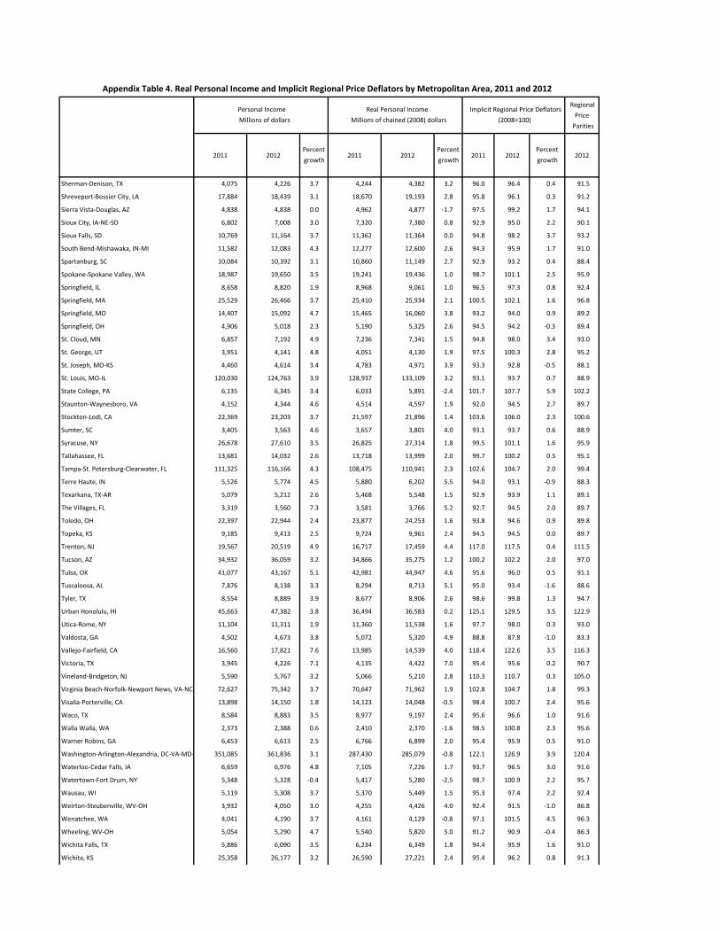
Regional

Price

Parities

2011 2012Percent

growth2011 2012

Percent

growth2011 2012

Percent

growth2012

Personal Income

Millions of dollars




(2008=100)


Sherman‐Denison, TX 4,075 4,226 3.7 4,244 4,382 3.2 96.0 96.4 0.4 91.5

Shreveport‐Bossier City, LA 17,884 18,439 3.1 18,670 19,193 2.8 95.8 96.1 0.3 91.2

Sierra Vista‐Douglas, AZ 4,838 4,838 0.0 4,962 4,877 ‐1.7 97.5 99.2 1.7 94.1

Sioux City, IA‐NE‐SD 6,802 7,008 3.0 7,320 7,380 0.8 92.9 95.0 2.2 90.1

Sioux Falls, SD 10,769 11,164 3.7 11,362 11,364 0.0 94.8 98.2 3.7 93.2

South Bend‐Mishawaka, IN‐MI 11,582 12,083 4.3 12,277 12,600 2.6 94.3 95.9 1.7 91.0

Spartanburg, SC 10,084 10,392 3.1 10,860 11,149 2.7 92.9 93.2 0.4 88.4

Spokane‐Spokane Valley, WA 18,987 19,650 3.5 19,241 19,436 1.0 98.7 101.1 2.5 95.9

Springfield, IL 8,658 8,820 1.9 8,968 9,061 1.0 96.5 97.3 0.8 92.4

Springfield, MA 25,529 26,466 3.7 25,410 25,934 2.1 100.5 102.1 1.6 96.8

Springfield, MO 14,407 15,092 4.7 15,465 16,060 3.8 93.2 94.0 0.9 89.2

Springfield, OH 4,906 5,018 2.3 5,190 5,325 2.6 94.5 94.2 ‐0.3 89.4

St. Cloud, MN 6,857 7,192 4.9 7,236 7,341 1.5 94.8 98.0 3.4 93.0

St. George, UT 3,951 4,141 4.8 4,051 4,130 1.9 97.5 100.3 2.8 95.2

St. Joseph, MO‐KS 4,460 4,614 3.4 4,783 4,971 3.9 93.3 92.8 ‐0.5 88.1

St. Louis, MO‐IL 120,030 124,763 3.9 128,937 133,109 3.2 93.1 93.7 0.7 88.9

State College, PA 6,135 6,345 3.4 6,033 5,891 ‐2.4 101.7 107.7 5.9 102.2

Staunton‐Waynesboro, VA 4,152 4,344 4.6 4,514 4,597 1.9 92.0 94.5 2.7 89.7

Stockton‐Lodi, CA 22,369 23,203 3.7 21,597 21,896 1.4 103.6 106.0 2.3 100.6

Sumter, SC 3,405 3,563 4.6 3,657 3,801 4.0 93.1 93.7 0.6 88.9

Syracuse, NY 26,678 27,610 3.5 26,825 27,314 1.8 99.5 101.1 1.6 95.9

Tallahassee, FL 13,681 14,032 2.6 13,718 13,999 2.0 99.7 100.2 0.5 95.1

Tampa‐St. Petersburg‐Clearwater, FL 111,325 116,166 4.3 108,475 110,941 2.3 102.6 104.7 2.0 99.4

Terre Haute, IN 5,526 5,774 4.5 5,880 6,202 5.5 94.0 93.1 ‐0.9 88.3

Texarkana, TX‐AR 5,079 5,212 2.6 5,468 5,548 1.5 92.9 93.9 1.1 89.1

The Villages, FL 3,319 3,560 7.3 3,581 3,766 5.2 92.7 94.5 2.0 89.7

Toledo, OH 22,397 22,944 2.4 23,877 24,253 1.6 93.8 94.6 0.9 89.8

Topeka, KS 9,185 9,413 2.5 9,724 9,961 2.4 94.5 94.5 0.0 89.7

Trenton, NJ 19,567 20,519 4.9 16,717 17,459 4.4 117.0 117.5 0.4 111.5

Tucson, AZ 34,932 36,059 3.2 34,866 35,275 1.2 100.2 102.2 2.0 97.0

Tulsa, OK 41,077 43,167 5.1 42,981 44,947 4.6 95.6 96.0 0.5 91.1

Tuscaloosa, AL 7,876 8,138 3.3 8,294 8,713 5.1 95.0 93.4 ‐1.6 88.6

Tyler, TX 8,554 8,889 3.9 8,677 8,906 2.6 98.6 99.8 1.3 94.7

Urban Honolulu, HI 45,663 47,382 3.8 36,494 36,583 0.2 125.1 129.5 3.5 122.9

Utica‐Rome, NY 11,104 11,311 1.9 11,360 11,538 1.6 97.7 98.0 0.3 93.0

Valdosta, GA 4,502 4,673 3.8 5,072 5,320 4.9 88.8 87.8 ‐1.0 83.3

Vallejo‐Fairfield, CA 16,560 17,821 7.6 13,985 14,539 4.0 118.4 122.6 3.5 116.3

Victoria, TX 3,945 4,226 7.1 4,135 4,422 7.0 95.4 95.6 0.2 90.7

Vineland‐Bridgeton, NJ 5,590 5,767 3.2 5,066 5,210 2.8 110.3 110.7 0.3 105.0

Virginia Beach‐Norfolk‐Newport News, VA‐NC 72,627 75,342 3.7 70,647 71,962 1.9 102.8 104.7 1.8 99.3

Visalia‐Porterville, CA 13,898 14,150 1.8 14,123 14,048 ‐0.5 98.4 100.7 2.4 95.6

Waco, TX 8,584 8,883 3.5 8,977 9,197 2.4 95.6 96.6 1.0 91.6

Walla Walla, WA 2,373 2,388 0.6 2,410 2,370 ‐1.6 98.5 100.8 2.3 95.6

Warner Robins, GA 6,453 6,613 2.5 6,766 6,899 2.0 95.4 95.9 0.5 91.0

Washington‐Arlington‐Alexandria, DC‐VA‐MD‐ 351,085 361,836 3.1 287,430 285,079 ‐0.8 122.1 126.9 3.9 120.4

Waterloo‐Cedar Falls, IA 6,659 6,976 4.8 7,105 7,226 1.7 93.7 96.5 3.0 91.6

Watertown‐Fort Drum, NY 5,348 5,328 ‐0.4 5,417 5,280 ‐2.5 98.7 100.9 2.2 95.7

Wausau, WI 5,119 5,308 3.7 5,370 5,449 1.5 95.3 97.4 2.2 92.4

Weirton‐Steubenville, WV‐OH 3,932 4,050 3.0 4,255 4,426 4.0 92.4 91.5 ‐1.0 86.8

Wenatchee, WA 4,041 4,190 3.7 4,161 4,129 ‐0.8 97.1 101.5 4.5 96.3

Wheeling, WV‐OH 5,054 5,290 4.7 5,540 5,820 5.0 91.2 90.9 ‐0.4 86.3

Wichita Falls, TX 5,886 6,090 3.5 6,234 6,349 1.8 94.4 95.9 1.6 91.0

Wichita, KS 25,358 26,177 3.2 26,590 27,221 2.4 95.4 96.2 0.8 91.3

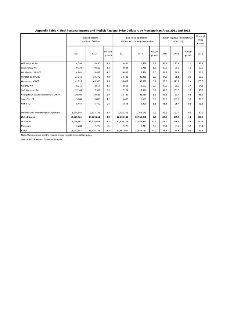
Regional

Price

Parities

2011 2012Percent

growth2011 2012

Percent

growth2011 2012

Percent

growth2012

Personal Income

Millions of dollars




(2008=100)


Williamsport, PA 4,298 4,480 4.3 4,481 4,578 2.2 95.9 97.9 2.0 92.9

Wilmington, NC 9,322 9,619 3.2 9,594 9,716 1.3 97.2 99.0 1.9 93.9

Winchester, VA‐WV 4,641 4,838 4.2 4,899 4,998 2.0 94.7 96.8 2.2 91.9

Winston‐Salem, NC 23,241 24,370 4.9 24,486 25,439 3.9 94.9 95.8 0.9 90.9

Worcester, MA‐CT 41,926 43,326 3.3 38,619 38,982 0.9 108.6 111.1 2.4 105.5

Yakima, WA 8,311 8,567 3.1 8,513 8,572 0.7 97.6 99.9 2.4 94.8

York‐Hanover, PA 17,188 17,568 2.2 17,264 17,316 0.3 99.6 101.5 1.9 96.3

Youngstown‐Warren‐Boardman, OH‐PA 19,308 19,682 1.9 20,735 21,010 1.3 93.1 93.7 0.6 88.9

Yuba City, CA 5,606 5,838 4.2 5,605 5,635 0.5 100.0 103.6 3.6 98.3

Yuma, AZ 5,487 5,400 ‐1.6 5,553 5,490 ‐1.1 98.8 98.4 ‐0.5 93.3

United States nonmetropolitan portion 1,574,840 1,633,732 3.7 1,708,781 1,763,271 3.2 92.2 92.7 0.5 87.9

United States 13,179,561 13,729,063 4.2 12,670,133 12,958,961 2.3 104.0 105.9 1.8 100.0

Maximum 13,179,561 13,729,063 12.1 12,670,133 12,958,961 10.2 126.4 129.5 5.9 122.9

Minimum 2,208 2,277 ‐1.6 2,226 2,243 ‐3.8 85.1 83.7 ‐3.6 79.4

Range 13,177,353 13,726,786 13.7 12,667,907 12,956,717 14.0 41.3 45.8 9.5 43.5

Note: The maximum and the minimum only include metropolitan areas.


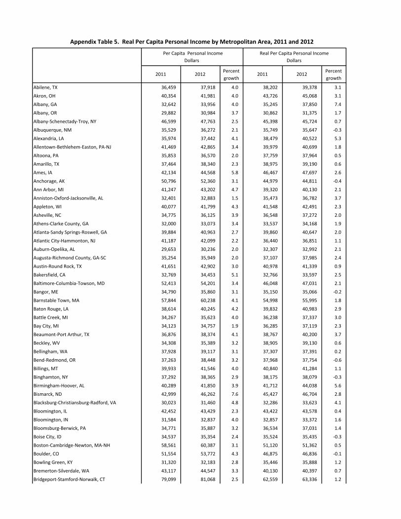
2011 2012Percent

growth2011 2012

Percent

growth

Abilene, TX 36,459 37,918 4.0 38,202 39,378 3.1

Akron, OH 40,354 41,981 4.0 43,726 45,068 3.1

Albany, GA 32,642 33,956 4.0 35,245 37,850 7.4

Albany, OR 29,882 30,984 3.7 30,862 31,375 1.7

Albany‐Schenectady‐Troy, NY 46,599 47,763 2.5 45,398 45,724 0.7

Albuquerque, NM 35,529 36,272 2.1 35,749 35,647 ‐0.3

Alexandria, LA 35,974 37,442 4.1 38,479 40,522 5.3

Allentown‐Bethlehem‐Easton, PA‐NJ 41,469 42,865 3.4 39,979 40,699 1.8

Altoona, PA 35,853 36,570 2.0 37,759 37,964 0.5

Amarillo, TX 37,464 38,340 2.3 38,975 39,190 0.6

Ames, IA 42,134 44,568 5.8 46,467 47,697 2.6

Anchorage, AK 50,796 52,360 3.1 44,979 44,811 ‐0.4

Ann Arbor, MI 41,247 43,202 4.7 39,320 40,130 2.1

Anniston‐Oxford‐Jacksonville, AL 32,401 32,883 1.5 35,473 36,782 3.7

Appleton, WI 40,077 41,799 4.3 41,548 42,491 2.3

Asheville, NC 34,775 36,125 3.9 36,548 37,272 2.0

Athens‐Clarke County, GA 32,000 33,073 3.4 33,537 34,168 1.9

Atlanta‐Sandy Springs‐Roswell, GA 39,884 40,963 2.7 39,860 40,647 2.0

Atlantic City‐Hammonton, NJ 41,187 42,099 2.2 36,440 36,851 1.1

Auburn‐Opelika, AL 29,653 30,236 2.0 32,307 32,992 2.1

Augusta‐Richmond County, GA‐SC 35,254 35,949 2.0 37,107 37,985 2.4

Austin‐Round Rock, TX 41,651 42,902 3.0 40,978 41,339 0.9

Bakersfield, CA 32,769 34,453 5.1 32,766 33,597 2.5

Baltimore‐Columbia‐Towson, MD 52,413 54,201 3.4 46,048 47,031 2.1

Bangor, ME 34,790 35,860 3.1 35,150 35,066 ‐0.2

Barnstable Town, MA 57,844 60,238 4.1 54,998 55,995 1.8

Baton Rouge, LA 38,614 40,245 4.2 39,832 40,983 2.9

Battle Creek, MI 34,267 35,623 4.0 36,238 37,337 3.0

Bay City, MI 34,123 34,757 1.9 36,285 37,119 2.3

Beaumont‐Port Arthur, TX 36,876 38,374 4.1 38,767 40,200 3.7

Beckley, WV 34,308 35,389 3.2 38,905 39,130 0.6

Bellingham, WA 37,928 39,117 3.1 37,307 37,391 0.2

Bend‐Redmond, OR 37,263 38,448 3.2 37,968 37,754 ‐0.6

Billings, MT 39,933 41,546 4.0 40,840 41,284 1.1

Binghamton, NY 37,292 38,365 2.9 38,175 38,079 ‐0.3

Birmingham‐Hoover, AL 40,289 41,850 3.9 41,712 44,038 5.6

Bismarck, ND 42,999 46,262 7.6 45,427 46,704 2.8

Blacksburg‐Christiansburg‐Radford, VA 30,023 31,460 4.8 32,286 33,623 4.1

Bloomington, IL 42,452 43,429 2.3 43,422 43,578 0.4

Bloomington, IN 31,584 32,837 4.0 32,857 33,372 1.6

Bloomsburg‐Berwick, PA 34,771 35,887 3.2 36,534 37,031 1.4

Boise City, ID 34,537 35,354 2.4 35,524 35,435 ‐0.3

Boston‐Cambridge‐Newton, MA‐NH 58,561 60,387 3.1 51,120 51,362 0.5

Boulder, CO 51,554 53,772 4.3 46,875 46,836 ‐0.1

Bowling Green, KY 31,320 32,183 2.8 35,446 35,888 1.2

Bremerton‐Silverdale, WA 43,117 44,547 3.3 40,130 40,397 0.7

Bridgeport‐Stamford‐Norwalk, CT 79,099 81,068 2.5 62,559 63,336 1.2

Appendix Table 5. Real Per Capita Personal Income by Metropolitan Area, 2011 and 2012


Dollars


Dollars

2011 2012Percent

growth2011 2012

Percent

growth



Dollars


Dollars

Brownsville‐Harlingen, TX 23,405 23,909 2.2 25,814 26,661 3.3

Brunswick, GA 33,428 34,478 3.1 37,139 37,996 2.3

Buffalo‐Cheektowaga‐Niagara Falls, NY 41,501 42,788 3.1 42,305 43,272 2.3

Burlington, NC 31,730 32,929 3.8 33,504 34,732 3.7

Burlington‐South Burlington, VT 45,525 47,285 3.9 43,241 43,876 1.5

California‐Lexington Park, MD 46,997 47,609 1.3 44,579 44,170 ‐0.9

Canton‐Massillon, OH 35,896 37,115 3.4 38,358 39,407 2.7

Cape Coral‐Fort Myers, FL 42,153 43,169 2.4 42,779 43,104 0.8

Cape Girardeau, MO‐IL 34,292 35,545 3.7 39,532 40,758 3.1

Carbondale‐Marion, IL 34,710 35,745 3.0 40,021 40,332 0.8

Carson City, NV 41,033 42,236 2.9 40,585 40,909 0.8

Casper, WY 55,608 57,522 3.4 55,543 55,828 0.5

Cedar Rapids, IA 42,678 44,131 3.4 45,112 45,895 1.7

Chambersburg‐Waynesboro, PA 35,743 36,743 2.8 36,036 36,369 0.9

Champaign‐Urbana, IL 37,987 39,086 2.9 39,110 39,495 1.0

Charleston, WV 40,945 42,329 3.4 43,453 44,721 2.9

Charleston‐North Charleston, SC 38,818 39,444 1.6 38,799 39,090 0.8

Charlotte‐Concord‐Gastonia, NC‐SC 38,911 40,465 4.0 39,869 40,706 2.1

Charlottesville, VA 44,748 46,667 4.3 43,745 44,671 2.1

Chattanooga, TN‐GA 35,899 37,228 3.7 38,054 39,051 2.6

Cheyenne, WY 49,443 50,755 2.7 49,868 50,004 0.3

Chicago‐Naperville‐Elgin, IL‐IN‐WI 46,305 48,305 4.3 42,304 42,984 1.6

Chico, CA 34,477 35,696 3.5 33,884 33,802 ‐0.2

Cincinnati, OH‐KY‐IN 41,738 43,454 4.1 43,583 45,047 3.4

Clarksville, TN‐KY 39,527 38,902 ‐1.6 41,690 40,627 ‐2.5

Cleveland, TN 31,544 33,148 5.1 35,687 37,891 6.2

Cleveland‐Elyria, OH 43,010 44,775 4.1 46,646 47,631 2.1

Coeur d'Alene, ID 33,631 34,656 3.0 34,837 35,205 1.1

College Station‐Bryan, TX 30,664 31,788 3.7 31,219 31,990 2.5

Colorado Springs, CO 40,105 40,980 2.2 39,601 39,431 ‐0.4

Columbia, MO 38,171 39,557 3.6 39,624 40,701 2.7

Columbia, SC 36,163 37,294 3.1 37,394 38,406 2.7

Columbus, GA‐AL 38,589 39,216 1.6 40,404 41,793 3.4

Columbus, IN 40,417 43,419 7.4 44,603 47,209 5.8

Columbus, OH 41,048 42,728 4.1 42,119 43,208 2.6

Corpus Christi, TX 39,262 40,796 3.9 40,427 41,797 3.4

Corvallis, OR 38,439 39,880 3.7 38,773 38,864 0.2

Crestview‐Fort Walton Beach‐Destin, FL 42,246 43,078 2.0 42,141 42,184 0.1

Cumberland, MD‐WV 33,277 34,431 3.5 35,605 37,035 4.0

Dallas‐Fort Worth‐Arlington, TX 44,628 46,136 3.4 42,606 43,327 1.7

Dalton, GA 27,701 28,548 3.1 31,368 31,861 1.6

Danville, IL 32,791 33,937 3.5 37,776 40,538 7.3

Daphne‐Fairhope‐Foley, AL 38,115 38,548 1.1 41,470 41,103 ‐0.9

Davenport‐Moline‐Rock Island, IA‐IL 42,836 43,847 2.4 45,065 45,196 0.3

Dayton, OH 38,736 39,891 3.0 40,513 41,596 2.7

Decatur, AL 32,185 33,127 2.9 34,859 36,162 3.7

Decatur, IL 41,021 42,287 3.1 43,356 44,757 3.2

2011 2012Percent

growth2011 2012

Percent

growth



Dollars


Dollars

Deltona‐Daytona Beach‐Ormond Beach, FL 33,475 34,661 3.5 33,793 34,439 1.9

Denver‐Aurora‐Lakewood, CO 49,119 50,936 3.7 46,226 46,337 0.2

Des Moines‐West Des Moines, IA 45,130 46,753 3.6 46,227 46,925 1.5

Detroit‐Warren‐Dearborn, MI 40,776 42,261 3.6 39,907 40,995 2.7

Dothan, AL 34,727 35,816 3.1 38,307 39,975 4.4

Dover, DE 35,077 36,155 3.1 35,580 36,468 2.5

Dubuque, IA 38,610 40,371 4.6 40,489 41,240 1.9

Duluth, MN‐WI 37,156 38,171 2.7 38,990 39,502 1.3

Durham‐Chapel Hill, NC 43,111 44,294 2.7 44,031 44,226 0.4

East Stroudsburg, PA 32,857 33,781 2.8 31,786 32,075 0.9

Eau Claire, WI 37,602 39,138 4.1 39,330 40,255 2.4

El Centro, CA 30,459 30,894 1.4 31,960 31,795 ‐0.5

El Paso, TX 29,315 30,186 3.0 31,356 31,544 0.6

Elizabethtown‐Fort Knox, KY 38,831 38,981 0.4 43,110 42,660 ‐1.0

Elkhart‐Goshen, IN 32,988 35,550 7.8 34,611 36,813 6.4

Elmira, NY 37,313 38,056 2.0 38,042 38,319 0.7

Erie, PA 35,972 36,671 1.9 37,288 37,403 0.3

Eugene, OR 34,614 35,941 3.8 34,681 34,891 0.6

Evansville, IN‐KY 39,176 40,437 3.2 40,930 42,446 3.7

Fairbanks, AK 44,851 45,432 1.3 41,207 40,354 ‐2.1

Fargo, ND‐MN 43,570 46,384 6.5 45,761 47,059 2.8

Farmington, NM 32,039 33,092 3.3 33,789 33,889 0.3

Fayetteville, NC 43,192 43,928 1.7 45,054 45,555 1.1

Fayetteville‐Springdale‐Rogers, AR‐MO 34,569 35,977 4.1 36,758 37,815 2.9

Flagstaff, AZ 34,430 34,820 1.1 34,095 33,566 ‐1.5

Flint, MI 31,426 32,421 3.2 31,789 32,804 3.2

Florence, SC 33,491 34,445 2.8 36,775 38,211 3.9

Florence‐Muscle Shoals, AL 32,233 33,249 3.2 35,236 37,331 5.9

Fond du Lac, WI 37,788 39,459 4.4 42,475 43,637 2.7

Fort Collins, CO 39,992 41,311 3.3 39,183 39,100 ‐0.2

Fort Smith, AR‐OK 32,651 33,876 3.8 35,883 37,570 4.7

Fort Wayne, IN 35,584 37,226 4.6 37,693 38,782 2.9

Fresno, CA 33,132 34,074 2.8 32,977 33,118 0.4

Gadsden, AL 31,851 32,717 2.7 34,689 36,647 5.6

Gainesville, FL 36,858 38,045 3.2 36,766 37,486 2.0

Gainesville, GA 32,288 32,789 1.6 34,724 34,338 ‐1.1

Gettysburg, PA 34,628 35,720 3.2 34,912 35,357 1.3

Glens Falls, NY 38,680 40,058 3.6 38,381 38,911 1.4

Goldsboro, NC 32,003 33,620 5.1 34,587 36,774 6.3

Grand Forks, ND‐MN 40,093 43,916 9.5 42,216 44,907 6.4

Grand Island, NE 39,835 41,395 3.9 46,110 46,387 0.6

Grand Junction, CO 34,681 35,726 3.0 35,049 35,640 1.7

Grand Rapids‐Wyoming, MI 35,845 37,264 4.0 37,496 38,293 2.1

Grants Pass, OR 30,416 31,361 3.1 31,413 31,756 1.1

Great Falls, MT 39,435 40,822 3.5 41,084 41,094 0.0

Greeley, CO 30,400 31,657 4.1 30,430 30,765 1.1

Green Bay, WI 40,497 41,609 2.7 42,576 42,877 0.7

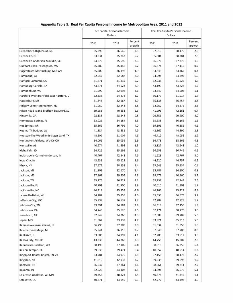
2011 2012Percent

growth2011 2012

Percent

growth



Dollars


Dollars

Greensboro‐High Point, NC 35,395 36,645 3.5 37,510 38,479 2.6

Greenville, NC 33,831 35,743 5.7 35,601 38,381 7.8

Greenville‐Anderson‐Mauldin, SC 34,879 35,696 2.3 36,676 37,278 1.6

Gulfport‐Biloxi‐Pascagoula, MS 35,380 35,448 0.2 36,874 37,115 0.7

Hagerstown‐Martinsburg, MD‐WV 35,509 36,196 1.9 33,343 33,467 0.4

Hammond, LA 32,047 32,687 2.0 34,994 34,897 ‐0.3

Hanford‐Corcoran, CA 31,771 31,835 0.2 32,238 31,626 ‐1.9

Harrisburg‐Carlisle, PA 43,271 44,523 2.9 43,199 43,726 1.2

Harrisonburg, VA 31,999 32,998 3.1 33,640 34,003 1.1

Hartford‐West Hartford‐East Hartford, CT 52,338 54,274 3.7 50,177 51,017 1.7

Hattiesburg, MS 31,346 32,567 3.9 35,138 36,457 3.8

Hickory‐Lenoir‐Morganton, NC 31,060 32,243 3.8 33,262 34,375 3.3

Hilton Head Island‐Bluffton‐Beaufort, SC 39,953 40,853 2.3 41,995 42,161 0.4

Hinesville, GA 28,136 28,348 0.8 29,851 29,200 ‐2.2

Homosassa Springs, FL 33,026 34,184 3.5 35,638 36,166 1.5

Hot Springs, AR 35,369 36,796 4.0 39,101 40,886 4.6

Houma‐Thibodaux, LA 41,584 43,631 4.9 43,569 44,699 2.6

Houston‐The Woodlands‐Sugar Land, TX 48,809 51,004 4.5 46,712 48,053 2.9

Huntington‐Ashland, WV‐KY‐OH 34,065 35,059 2.9 36,778 38,362 4.3

Huntsville, AL 40,974 41,595 1.5 42,827 43,243 1.0

Idaho Falls, ID 34,726 35,292 1.6 36,658 36,745 0.2

Indianapolis‐Carmel‐Anderson, IN 40,467 42,342 4.6 41,529 42,767 3.0

Iowa City, IA 43,631 45,222 3.6 44,520 44,757 0.5

Ithaca, NY 37,579 38,852 3.4 35,541 35,334 ‐0.6

Jackson, MI 31,902 32,670 2.4 33,787 34,100 0.9

Jackson, MS 37,861 39,505 4.3 39,479 40,960 3.7

Jackson, TN 35,276 36,721 4.1 39,737 42,744 7.6

Jacksonville, FL 40,701 41,900 2.9 40,610 41,301 1.7

Jacksonville, NC 46,418 45,953 ‐1.0 46,766 45,422 ‐2.9

Janesville‐Beloit, WI 34,282 35,855 4.6 35,533 36,673 3.2

Jefferson City, MO 35,939 36,537 1.7 42,207 42,928 1.7

Johnson City, TN 33,591 34,582 2.9 36,513 37,156 1.8

Johnstown, PA 34,749 35,620 2.5 37,471 38,776 3.5

Jonesboro, AR 32,849 34,266 4.3 37,688 39,789 5.6

Joplin, MO 31,662 33,139 4.7 33,921 35,813 5.6

Kahului‐Wailuku‐Lahaina, HI 36,790 37,909 3.0 31,534 31,859 1.0

Kalamazoo‐Portage, MI 35,944 36,916 2.7 37,548 37,783 0.6

Kankakee, IL 33,603 34,997 4.1 32,283 33,512 3.8

Kansas City, MO‐KS 43,330 44,766 3.3 44,755 45,802 2.3

Kennewick‐Richland, WA 38,195 37,109 ‐2.8 38,318 36,255 ‐5.4

Killeen‐Temple, TX 39,630 39,471 ‐0.4 40,857 40,514 ‐0.8

Kingsport‐Bristol‐Bristol, TN‐VA 33,781 34,975 3.5 37,155 38,173 2.7

Kingston, NY 41,619 42,937 3.2 39,235 39,693 1.2

Knoxville, TN 36,537 37,864 3.6 38,361 39,211 2.2

Kokomo, IN 32,626 34,107 4.5 34,894 36,676 5.1

La Crosse‐Onalaska, WI‐MN 39,456 40,824 3.5 40,878 41,347 1.1

Lafayette, LA 40,871 43,049 5.3 42,777 44,493 4.0

2011 2012Percent

growth2011 2012

Percent

growth



Dollars


Dollars

Lafayette‐West Lafayette, IN 32,739 33,822 3.3 33,746 34,175 1.3

Lake Charles, LA 35,568 37,226 4.7 38,090 39,912 4.8

Lake Havasu City‐Kingman, AZ 26,524 27,220 2.6 27,170 27,546 1.4

Lakeland‐Winter Haven, FL 34,630 35,746 3.2 35,269 36,116 2.4

Lancaster, PA 39,013 40,088 2.8 38,913 38,600 ‐0.8

Lansing‐East Lansing, MI 34,712 35,459 2.2 35,671 35,633 ‐0.1

Laredo, TX 25,612 26,120 2.0 26,949 27,871 3.4

Las Cruces, NM 30,488 30,862 1.2 31,814 31,663 ‐0.5

Las Vegas‐Henderson‐Paradise, NV 35,896 36,676 2.2 34,663 35,053 1.1

Lawrence, KS 35,268 36,331 3.0 35,610 36,103 1.4

Lawton, OK 36,969 36,992 0.1 38,716 38,380 ‐0.9

Lebanon, PA 40,427 41,268 2.1 41,275 41,267 0.0

Lewiston, ID‐WA 36,011 37,080 3.0 38,369 38,376 0.0

Lewiston‐Auburn, ME 36,246 37,018 2.1 37,249 36,956 ‐0.8

Lexington‐Fayette, KY 38,836 39,925 2.8 40,574 41,112 1.3

Lima, OH 32,034 33,044 3.2 34,589 35,215 1.8

Lincoln, NE 40,015 41,584 3.9 42,115 42,482 0.9

Little Rock‐North Little Rock‐Conway, AR 40,346 41,662 3.3 41,851 43,397 3.7

Logan, UT‐ID 28,731 29,243 1.8 30,358 30,545 0.6

Longview, TX 39,788 41,945 5.4 41,864 43,332 3.5

Longview, WA 33,261 34,867 4.8 34,756 35,153 1.1

Los Angeles‐Long Beach‐Anaheim, CA 44,768 46,337 3.5 37,491 37,192 ‐0.8

Louisville/Jefferson County, KY‐IN 39,241 40,970 4.4 41,380 42,751 3.3

Lubbock, TX 34,545 36,074 4.4 35,630 36,502 2.4

Lynchburg, VA 34,334 35,243 2.6 36,072 36,896 2.3

Macon, GA 36,015 36,879 2.4 38,211 39,781 4.1

Madera, CA 29,790 31,169 4.6 30,124 30,692 1.9

Madison, WI 46,479 48,026 3.3 46,566 46,570 0.0

Manchester‐Nashua, NH 49,169 50,806 3.3 43,948 44,249 0.7

Manhattan, KS 43,129 42,464 ‐1.5 45,659 43,852 ‐4.0

Mankato‐North Mankato, MN 38,055 40,052 5.2 42,156 43,041 2.1

Mansfield, OH 31,642 32,437 2.5 34,199 34,669 1.4

McAllen‐Edinburg‐Mission, TX 22,127 22,400 1.2 24,399 25,008 2.5

Medford, OR 34,907 36,289 4.0 34,818 35,135 0.9

Memphis, TN‐MS‐AR 38,637 40,288 4.3 39,786 41,499 4.3

Merced, CA 29,995 30,630 2.1 30,461 30,355 ‐0.3

Miami‐Fort Lauderdale‐West Palm Beach, FL 43,106 44,222 2.6 40,116 39,963 ‐0.4

Michigan City‐La Porte, IN 32,026 33,399 4.3 36,388 37,534 3.1

Midland, MI 44,739 45,423 1.5 50,049 49,615 ‐0.9

Midland, TX 77,495 83,049 7.2 76,841 80,504 4.8

Milwaukee‐Waukesha‐West Allis, WI 45,477 46,943 3.2 46,424 46,771 0.7

Minneapolis‐St. Paul‐Bloomington, MN‐WI 48,857 50,260 2.9 46,475 46,296 ‐0.4

Missoula, MT 35,342 36,584 3.5 36,022 35,986 ‐0.1

Mobile, AL 32,580 32,772 0.6 34,242 35,256 3.0

Modesto, CA 33,005 34,138 3.4 32,274 32,704 1.3

Monroe, LA 34,014 35,482 4.3 36,653 38,587 5.3

Monroe, MI 36,227 38,401 6.0 35,846 37,687 5.1

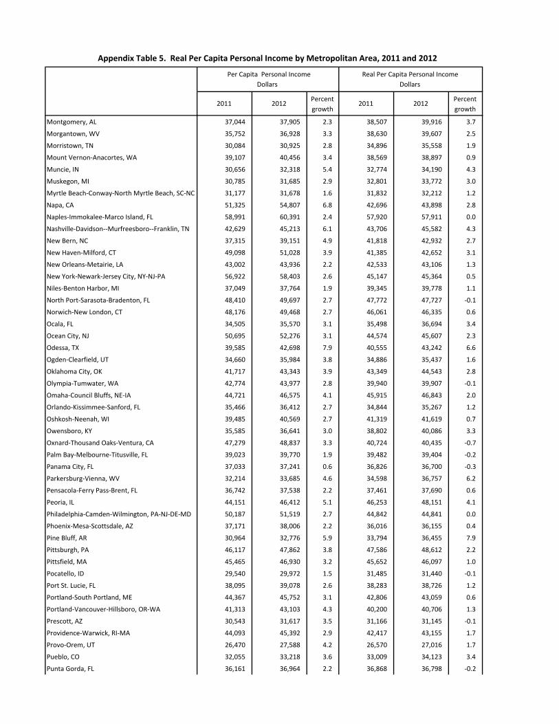
2011 2012Percent

growth2011 2012

Percent

growth



Dollars


Dollars

Montgomery, AL 37,044 37,905 2.3 38,507 39,916 3.7

Morgantown, WV 35,752 36,928 3.3 38,630 39,607 2.5

Morristown, TN 30,084 30,925 2.8 34,896 35,558 1.9

Mount Vernon‐Anacortes, WA 39,107 40,456 3.4 38,569 38,897 0.9

Muncie, IN 30,656 32,318 5.4 32,774 34,190 4.3

Muskegon, MI 30,785 31,685 2.9 32,801 33,772 3.0

Myrtle Beach‐Conway‐North Myrtle Beach, SC‐NC 31,177 31,678 1.6 31,832 32,212 1.2

Napa, CA 51,325 54,807 6.8 42,696 43,898 2.8

Naples‐Immokalee‐Marco Island, FL 58,991 60,391 2.4 57,920 57,911 0.0

Nashville‐Davidson‐‐Murfreesboro‐‐Franklin, TN 42,629 45,213 6.1 43,706 45,582 4.3

New Bern, NC 37,315 39,151 4.9 41,818 42,932 2.7

New Haven‐Milford, CT 49,098 51,028 3.9 41,385 42,652 3.1

New Orleans‐Metairie, LA 43,002 43,936 2.2 42,533 43,106 1.3

New York‐Newark‐Jersey City, NY‐NJ‐PA 56,922 58,403 2.6 45,147 45,364 0.5

Niles‐Benton Harbor, MI 37,049 37,764 1.9 39,345 39,778 1.1

North Port‐Sarasota‐Bradenton, FL 48,410 49,697 2.7 47,772 47,727 ‐0.1

Norwich‐New London, CT 48,176 49,468 2.7 46,061 46,335 0.6

Ocala, FL 34,505 35,570 3.1 35,498 36,694 3.4

Ocean City, NJ 50,695 52,276 3.1 44,574 45,607 2.3

Odessa, TX 39,585 42,698 7.9 40,555 43,242 6.6

Ogden‐Clearfield, UT 34,660 35,984 3.8 34,886 35,437 1.6

Oklahoma City, OK 41,717 43,343 3.9 43,349 44,543 2.8

Olympia‐Tumwater, WA 42,774 43,977 2.8 39,940 39,907 ‐0.1

Omaha‐Council Bluffs, NE‐IA 44,721 46,575 4.1 45,915 46,843 2.0

Orlando‐Kissimmee‐Sanford, FL 35,466 36,412 2.7 34,844 35,267 1.2

Oshkosh‐Neenah, WI 39,485 40,569 2.7 41,319 41,619 0.7

Owensboro, KY 35,585 36,641 3.0 38,802 40,086 3.3

Oxnard‐Thousand Oaks‐Ventura, CA 47,279 48,837 3.3 40,724 40,435 ‐0.7

Palm Bay‐Melbourne‐Titusville, FL 39,023 39,770 1.9 39,482 39,404 ‐0.2

Panama City, FL 37,033 37,241 0.6 36,826 36,700 ‐0.3

Parkersburg‐Vienna, WV 32,214 33,685 4.6 34,598 36,757 6.2

Pensacola‐Ferry Pass‐Brent, FL 36,742 37,538 2.2 37,461 37,690 0.6

Peoria, IL 44,151 46,412 5.1 46,253 48,151 4.1

Philadelphia‐Camden‐Wilmington, PA‐NJ‐DE‐MD 50,187 51,519 2.7 44,842 44,841 0.0

Phoenix‐Mesa‐Scottsdale, AZ 37,171 38,006 2.2 36,016 36,155 0.4

Pine Bluff, AR 30,964 32,776 5.9 33,794 36,455 7.9

Pittsburgh, PA 46,117 47,862 3.8 47,586 48,612 2.2

Pittsfield, MA 45,465 46,930 3.2 45,652 46,097 1.0

Pocatello, ID 29,540 29,972 1.5 31,485 31,440 ‐0.1

Port St. Lucie, FL 38,095 39,078 2.6 38,283 38,726 1.2

Portland‐South Portland, ME 44,367 45,752 3.1 42,806 43,059 0.6

Portland‐Vancouver‐Hillsboro, OR‐WA 41,313 43,103 4.3 40,200 40,706 1.3

Prescott, AZ 30,543 31,617 3.5 31,166 31,145 ‐0.1

Providence‐Warwick, RI‐MA 44,093 45,392 2.9 42,417 43,155 1.7

Provo‐Orem, UT 26,470 27,588 4.2 26,570 27,016 1.7

Pueblo, CO 32,055 33,218 3.6 33,009 34,123 3.4

Punta Gorda, FL 36,161 36,964 2.2 36,868 36,798 ‐0.2

2011 2012Percent

growth2011 2012

Percent

growth



Dollars


Dollars

Racine, WI 39,268 40,510 3.2 40,702 41,146 1.1

Raleigh, NC 41,276 42,709 3.5 41,824 42,580 1.8

Rapid City, SD 41,675 42,669 2.4 44,339 43,832 ‐1.1

Reading, PA 39,330 40,453 2.9 39,311 39,654 0.9

Redding, CA 36,507 37,593 3.0 35,931 36,180 0.7

Reno, NV 42,524 43,317 1.9 41,312 41,329 0.0

Richmond, VA 43,856 45,194 3.1 43,997 44,491 1.1

Riverside‐San Bernardino‐Ontario, CA 31,096 31,900 2.6 28,643 28,472 ‐0.6

Roanoke, VA 39,394 40,769 3.5 41,506 42,382 2.1

Rochester, MN 43,846 45,702 4.2 45,417 46,278 1.9

Rochester, NY 42,313 43,780 3.5 42,022 42,527 1.2

Rockford, IL 34,962 36,359 4.0 36,191 37,555 3.8

Rocky Mount, NC 31,754 32,964 3.8 33,649 36,021 7.1

Rome, GA 33,322 34,230 2.7 37,142 39,491 6.3

Sacramento‐‐Roseville‐‐Arden‐Arcade, CA 43,094 44,641 3.6 41,115 41,371 0.6

Saginaw, MI 32,457 33,079 1.9 34,214 35,105 2.6

Salem, OR 33,801 34,711 2.7 33,940 34,041 0.3

Salinas, CA 41,906 43,034 2.7 38,613 38,111 ‐1.3

Salisbury, MD‐DE 37,402 38,467 2.8 39,405 40,558 2.9

Salt Lake City, UT 38,883 40,424 4.0 38,197 38,705 1.3

San Angelo, TX 38,845 39,711 2.2 40,645 40,931 0.7

San Antonio‐New Braunfels, TX 38,124 39,019 2.3 39,128 39,436 0.8

San Diego‐Carlsbad, CA 48,066 49,719 3.4 40,246 39,657 ‐1.5

San Francisco‐Oakland‐Hayward, CA 62,954 66,591 5.8 51,279 52,105 1.6

San Jose‐Sunnyvale‐Santa Clara, CA 61,831 65,679 6.2 50,322 51,095 1.5

San Luis Obispo‐Paso Robles‐Arroyo Grande, CA 42,394 43,698 3.1 39,097 38,806 ‐0.7

Santa Cruz‐Watsonville, CA 50,138 52,442 4.6 41,288 40,992 ‐0.7

Santa Fe, NM 43,086 44,098 2.3 42,072 42,172 0.2

Santa Maria‐Santa Barbara, CA 46,210 47,862 3.6 41,908 41,956 0.1

Santa Rosa, CA 45,805 47,879 4.5 38,397 38,433 0.1

Savannah, GA 40,306 40,697 1.0 40,591 40,676 0.2

Scranton‐‐Wilkes‐Barre‐‐Hazleton, PA 38,188 39,101 2.4 39,389 40,306 2.3

Seattle‐Tacoma‐Bellevue, WA 51,250 53,328 4.1 46,685 47,290 1.3

Sebastian‐Vero Beach, FL 51,041 52,855 3.6 53,959 54,625 1.2

Sebring, FL 30,434 31,076 2.1 32,841 32,879 0.1

Sheboygan, WI 42,748 44,779 4.8 45,123 46,656 3.4

Sherman‐Denison, TX 33,595 34,655 3.2 34,987 35,936 2.7

Shreveport‐Bossier City, LA 40,199 41,234 2.6 41,966 42,918 2.3

Sierra Vista‐Douglas, AZ 36,437 36,625 0.5 37,370 36,922 ‐1.2

Sioux City, IA‐NE‐SD 40,261 41,485 3.0 43,328 43,687 0.8

Sioux Falls, SD 46,329 47,057 1.6 48,880 47,897 ‐2.0

South Bend‐Mishawaka, IN‐MI 36,279 37,929 4.5 38,458 39,549 2.8

Spartanburg, SC 32,025 32,784 2.4 34,488 35,172 2.0

Spokane‐Spokane Valley, WA 35,831 36,918 3.0 36,311 36,517 0.6

Springfield, IL 40,901 41,606 1.7 42,366 42,740 0.9

Springfield, MA 40,823 42,298 3.6 40,633 41,446 2.0

Springfield, MO 32,721 33,943 3.7 35,123 36,121 2.8

2011 2012Percent

growth2011 2012

Percent

growth



Dollars


Dollars

Springfield, OH 35,609 36,572 2.7 37,670 38,812 3.0

St. Cloud, MN 36,080 37,756 4.6 38,075 38,540 1.2

St. George, UT 27,920 28,597 2.4 28,629 28,518 ‐0.4

St. Joseph, MO‐KS 34,943 36,068 3.2 37,470 38,855 3.7

St. Louis, MO‐IL 42,969 44,625 3.9 46,158 47,610 3.1

State College, PA 39,651 40,894 3.1 38,991 37,962 ‐2.6

Staunton‐Waynesboro, VA 34,918 36,597 4.8 37,954 38,734 2.1

Stockton‐Lodi, CA 32,157 33,024 2.7 31,047 31,163 0.4

Sumter, SC 31,725 32,973 3.9 34,066 35,180 3.3

Syracuse, NY 40,273 41,774 3.7 40,494 41,327 2.1

Tallahassee, FL 36,874 37,382 1.4 36,973 37,294 0.9

Tampa‐St. Petersburg‐Clearwater, FL 39,387 40,862 3.7 38,379 39,024 1.7

Terre Haute, IN 32,021 33,473 4.5 34,072 35,954 5.5

Texarkana, TX‐AR 33,949 34,819 2.6 36,546 37,062 1.4

The Villages, FL 33,782 35,032 3.7 36,453 37,064 1.7

Toledo, OH 36,758 37,693 2.5 39,186 39,843 1.7

Topeka, KS 39,130 40,132 2.6 41,426 42,467 2.5

Trenton, NJ 53,271 55,714 4.6 45,513 47,404 4.2

Tucson, AZ 35,371 36,335 2.7 35,304 35,545 0.7

Tulsa, OK 43,450 45,350 4.4 45,464 47,220 3.9

Tuscaloosa, AL 34,012 34,870 2.5 35,816 37,335 4.2

Tyler, TX 40,185 41,379 3.0 40,765 41,458 1.7

Urban Honolulu, HI 47,252 48,529 2.7 37,764 37,468 ‐0.8

Utica‐Rome, NY 37,166 37,949 2.1 38,024 38,710 1.8

Valdosta, GA 31,636 32,372 2.3 35,640 36,855 3.4

Vallejo‐Fairfield, CA 39,719 42,354 6.6 33,542 34,554 3.0

Victoria, TX 41,666 43,735 5.0 43,675 45,771 4.8

Vineland‐Bridgeton, NJ 35,560 36,551 2.8 32,225 33,021 2.5

Virginia Beach‐Norfolk‐Newport News, VA‐NC 43,051 44,321 2.9 41,878 42,332 1.1

Visalia‐Porterville, CA 31,027 31,307 0.9 31,531 31,081 ‐1.4

Waco, TX 33,576 34,657 3.2 35,115 35,882 2.2

Walla Walla, WA 37,371 37,674 0.8 37,951 37,390 ‐1.5

Warner Robins, GA 35,139 35,654 1.5 36,841 37,194 1.0

Washington‐Arlington‐Alexandria, DC‐VA‐MD‐WV 60,834 61,743 1.5 49,804 48,645 ‐2.3

Waterloo‐Cedar Falls, IA 39,587 41,339 4.4 42,234 42,824 1.4

Watertown‐Fort Drum, NY 45,260 44,301 ‐2.1 45,844 43,907 ‐4.2

Wausau, WI 38,048 39,399 3.5 39,911 40,439 1.3

Weirton‐Steubenville, WV‐OH 31,881 33,052 3.7 34,506 36,116 4.7

Wenatchee, WA 36,069 37,067 2.8 37,137 36,526 ‐1.6

Wheeling, WV‐OH 34,349 36,131 5.2 37,651 39,748 5.6

Wichita Falls, TX 39,217 40,379 3.0 41,536 42,092 1.3

Wichita, KS 40,039 41,152 2.8 41,983 42,793 1.9

Williamsport, PA 36,833 38,239 3.8 38,401 39,070 1.7

Wilmington, NC 35,933 36,514 1.6 36,979 36,885 ‐0.3

Winchester, VA‐WV 35,725 36,955 3.4 37,714 38,176 1.2

Winston‐Salem, NC 36,067 37,625 4.3 37,999 39,277 3.4

Worcester, MA‐CT 45,473 46,902 3.1 41,886 42,199 0.7

2011 2012Percent

growth2011 2012

Percent

growth



Dollars


Dollars

Yakima, WA 33,763 34,686 2.7 34,582 34,707 0.4

York‐Hanover, PA 39,329 40,124 2.0 39,502 39,549 0.1

Youngstown‐Warren‐Boardman, OH‐PA 34,374 35,260 2.6 36,914 37,638 2.0

Yuba City, CA 33,467 34,763 3.9 33,460 33,553 0.3

Yuma, AZ 27,385 26,995 ‐1.4 27,712 27,447 ‐1.0

United States nonmetropolitan portion 34,018 35,324 3.8 36,911 38,125 3.3

United States 42,298 43,735 3.4 40,663 41,282 1.5

Maximum 79,099 83,049 9.5 76,841 80,504 7.9

Minimum 22,127 22,400 ‐2.8 24,399 25,008 ‐5.4

Range 56,972 60,649 12.4 52,442 55,495 13.3


Regional Price Parities and Real Regional Income for … · Regional Price Parities and Real...

Documents

Transcript of Regional Price Parities and Real Regional Income for … · Regional Price Parities and Real...