www.environment.sa.gov.au

Protecting the harlequin fish within South Australia’s new system of marine parks: acoustic tracking to determine site fidelity and movement patterns Technical Report 2012/06

Protecting the harlequin fish within South Australia’s new system of marine parks: acoustic tracking to determine site

fidelity and movement patterns Final Report to the Department of Environment, Water and Natural Resources

Wildlife Conservation Fund Project Number 1455 2012

Simon Bryars1,3, Paul Rogers2, and David Miller1

1Department of Environment, Water and Natural Resources, 1 Richmond Rd, Keswick, SA 5035 2South Australian Research and Development Institute, 2 Hamra Ave, West Beach, SA 5024 &

Flinders University of South Australia, Sturt Road, Bedford Park, SA 5042 3Current address: PO Box 67, Verdun, SA 5245

DEWNR Technical Report 2012/06

This publication may be cited as: Bryars, S., Rogers, P., and Miller, D. (2012) Protecting the harlequin fish within South Australia’s new system of marine parks: acoustic tracking to determine site fidelity and movement patterns. Report to the Department of Environment, Water and Natural Resources Wildlife Conservation Fund Project Number 1455. Department of Environment, Water and Natural Resources. Adelaide. Photograph: Harlequin Fish No. 5 used in the tracking study. Photo credit: Simon Bryars Department of Environment, Water and Natural Resources GPO Box 1047 Adelaide SA 5001 http://www.environment.sa.gov.au © State of South Australia through the Department of Environment, Water and Natural Resources. Apart from fair dealings and other uses permitted by the Copyright Act 1968 (Cth), no part of this publication may be reproduced, published, communicated, transmitted, modified or commercialised without the prior written permission of the Department of Environment, Water and Natural Resources.

Disclaimer While reasonable efforts have been made to ensure the contents of this publication are factually correct, the Department of Environment, Water and Natural Resources makes no representations and accepts no responsibility for the accuracy, completeness or fitness for any particular purpose of the contents, and shall not be liable for any loss or damage that may be occasioned directly or indirectly through the use of or reliance on the contents of this publication. Reference to any company, product or service in this publication should not be taken as a Departmental endorsement of the company, product or service.

1

Acknowledgements

This project was financially supported by the Department of Environment, Water and

Natural Resources (DEWNR) Wildlife Conservation Fund (Project No 1455), the

DEWNR Coast & Marine Conservation Branch, and the DEWNR Nature

Conservation Branch. In-kind support was provided by the South Australian

Research and Development Institute (SARDI) Aquatic Sciences, and the Flinders

University of South Australia. Thanks to the following DEWNR staff who assisted with

the project: Dimitri Colella, Henry Rutherford, James Brook, Peter Copley, Dr Bryan

McDonald, Chris Thomas, Robyn Morcom and Alison Wright. Thanks also to Dr

Charlie Huveneers (SARDI and Flinders University of SA), Gavin Solly (KI Fishing

Adventures) and Dr Nicholas Payne (University of New South Wales) for technical

assistance. The project had Animal Ethics approval from the SA Wildlife Ethics

Committee (No. 35-2008-M4). Dr Brad Page, Patricia von Baumgarten, Rosemary

Paxinos, and Andrew Burnell (all from DEWNR) reviewed a draft version of the report

and provided constructive comments that greatly improved the final report.

2

Summary

An acoustic telemetry study aimed at tracking the movements of the harlequin fish

(Othos dentex) was undertaken off Kangaroo Island, South Australia. Seven acoustic

receivers were deployed in a near-linear array 400 m apart on the sandy seabed

adjacent to a narrow strip of high profile coastal reef. Ten harlequin fish (330–620

mm total length; 0.5–3 kg weight) were captured within the middle part of the array,

implanted with an acoustic transmitter, and then released at their point of capture.

Presence-absence and depth data were then passively monitored by the receiver

array over a 16-month period during 2010–11. Results showed that the harlequin fish

is a site-attached, diurnal predator, with a relatively small home range. These

characteristics, which had not been demonstrated previously, make individuals of the

species amenable to long-term day-time monitoring techniques and to a high level of

protection from localised impacts inside adequately-sized and appropriately-located

sanctuary zones within South Australia’s new system of marine parks. Nonetheless,

despite their high site fidelity, five of the fish underwent a coordinated alongshore

movement during which they moved rapidly >800 m to the eastern extreme of the

array. Three of the fish then returned to their original home range in the middle part

of the array, one fish disappeared from the array, and the other fish permanently

relocated its home range by ~800 m to the eastern end of the array. While it is most

likely that the temporary movement was related to an unusual storm event, if such

movements do occur regularly in this and other populations, the size requirements of

sanctuary zones need to take them into account.

3

Introduction

The harlequin fish (Othos dentex) is a reef species that inhabits shallow (<30 m

depth) temperate waters from south-western Western Australia (WA) to western

Victoria (Gomon et al. 2008). It prefers high profile reefs with drop-offs, crevices and

caves in clear coastal waters (Kuiter 1999, Gomon et al. 2008). The harlequin fish is

a member of the Serranidae family which includes groupers and cods. It is the only

member of its genus. The harlequin fish is superficially similar in size and shape to

the tropical serranid, the coral trout (Plectropomus leopardus). However, unlike in

tropical waters there are relatively few serranid species in the cold temperate waters

of South Australia (SA) where the harlequin fish is the largest serranid, reaching a

total length (TL) of 76 cm (Gomon et al. 2008, Hutchins and Swainston 2002). There

is very limited information available on the biology and ecology of the harlequin fish.

Harlequin fish may live to at least 42 years of age (Saunders et al. 2010). Size and

age at maturity are unknown. While many tropical serranids are protogynous

hermaphrodites (DeLoach and Humann 1999), there is no evidence of this occurring

in the harlequin fish (Saunders et al. 2010). The harlequin fish is thought to be site-

attached (Bryars 2011, Baker 2012), but again, limited data are available to support

this hypothesis. The harlequin fish is rarely seen by divers when compared to many

other reef fishes in SA, with only a few ‘hot-spots’ where sightings are more common

(S. Bryars, unpublished data). The lack of sightings may be partly related to its

cryptic nature; however, harlequin fish can be inquisitive and may follow or be easily

approached by divers (Kuiter 1999, Edgar 2008). The harlequin fish has a bottom-

dwelling habit whereby it regularly rests on the seabed (Edgar 2008) in between

short bursts of swimming or ‘hovering’ just above the seabed (S Bryars, pers. obs.).

Anecdotal observations indicate that it is a lie-in-wait ambush predator, and limited

gut content analyses show that small wrasses and leatherjackets are components of

its diet (Saunders et al. 2010, S Bryars, unpublished data). Crustaceans and

cephalopods may also be part of the harlequin fish diet as these are eaten more

broadly by serranids (Gomon et al. 2008).

The harlequin fish is incidentally captured on hook and line by commercial (Fowler et

al. 2009), recreational (pers. obs.), and charter boat fishers (Saunders et al. 2010). It

is also targeted by recreational spearfishers, and taken as bycatch in commercial and

recreational lobster pots (Baker 2012). There is little protection for harlequin fish

within SA, with no limits on recreational take and few limits on commercial take.

4

Coastal habitat degradation may also be a threat in some regions (Baker 2012).

Indeed the disappearance of the harlequin fish from Port Phillip Bay in Victoria has

been linked to poor water quality (Gomon 2001). Consequently the harlequin fish is

considered by some sectors to be of conservation concern in SA (Baker 2012). The

harlequin fish is one of a number of reef fishes for which reef survey data (along with

many other datasets) were utilised to inform the zoning process within South

Australia’s new system of 19 multiple-use marine parks (e.g., DENR 2010).

If harlequin fish are site-attached, then no-take sanctuary zones may offer a high

level of protection from localised impacts. However, it is imperative that sanctuary

zones are sufficiently large enough to encompass functioning populations of

individuals. Acoustic telemetry is a proven methodology for determining site fidelity

and home range size in reef fishes through tagging and tracking of movements over

spatial scales of kilometres and temporal scales of months to years (e.g. Tolimieri et

al. 2009, Green and Starr 2011, Bryars et al. 2012). Results obtained with this

technology have been used to discuss the effectiveness and performance of marine

parks for the conservation of reef fishes (e.g. Lowe et al. 2003, Topping et al. 2005,

Parsons et al. 2010).

In the present study we used acoustic telemetry to investigate if adult harlequin fish

are site-attached and if they have potential for a high level of protection within

adequately-sized sanctuary zones. Specific aims of the study were to: (1) determine

long-term site fidelity and home range, (2) investigate long-term movement patterns,

and (3) relate movement patterns to environmental and physical factors.

5

Materials and Methods

Field site

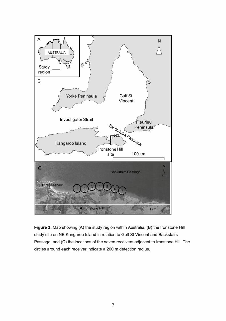
The study site was located to the east of Penneshaw adjacent to Ironstone Hill in

Backstairs Passage off NE Kangaroo Island, South Australia (Fig. 1). The Ironstone

Hill site is characterised by a relatively narrow strip of high-relief coastal reef (<50 m

width) that slopes steeply from cliffs into a relatively flat area at ~12–14 m depth

(Figs. 1, 2). The flatter area adjacent to the reef is characterised by a mixture of

sparse seagrass, bare sand, and patchy low-relief reef with sponges and other filter-

feeding invertebrates. Harlequin fish inhabit the strip of high-relief reef. While the tidal

amplitude at the site is only ~1.5 m, the site does experience relatively high

alongshore tidal flows due to the orientation of the coastline and the volume of water

flow in and out of Gulf St Vincent through the relatively narrow Backstairs Passage

(Bye and Kämpf 2008, Fig. 1).

Tracking equipment

A total of seven VEMCO® (VEMCO Division AMIRIX Systems Inc., Nova Scotia,

Canada) VR2W acoustic receivers were deployed at the field site, and a total of ten

individually-coded VEMCO® acoustic transmitters (V13P-1H, 13 mm diameter, 45

mm length, 12 g weight in air, 6 g weight in water) were surgically implanted in ten

fish. The fish transmitters were set with a minimum and maximum delay of 110 and

250 seconds, respectively, with a nominal delay of 180 seconds. All fish transmitters

were fitted with pressure sensors set for a depth range of 0–50 m, which covered the

range of depths found at the study site and was used to determine (1) if fish were

moving offshore away from the reef and into deeper water habitats outside of the

receiver array, and (2) how fish utilised the reef slope. Fish transmitters had an

estimated battery life of 511 days.

A single control VEMCO® transmitter (V13-1H, 13 mm diameter, 45 mm length) was

also deployed at the field site for the duration of the study. The control transmitter

was set with a minimum and maximum delay of 300 and 900 seconds, respectively,

with a nominal delay of 600 seconds. The control transmitter was used to aid

interpretation of fish transmitter data (see Transmitter deployment).

6

AUSTRALIA

A

Kangaroo Island

Yorke Peninsula

FleurieuPeninsula

Gulf StVincent

Investigator Strait

100 km

N

Study region

Ironstone Hill site

B

7

Penneshaw

Ironstone Hill

Backstairs Passage

N

1 km

231 6

54

C

Figure 1. Map showing (A) the study region within Australia, (B) the Ironstone Hill

study site on NE Kangaroo Island in relation to Gulf St Vincent and Backstairs

Passage, and (C) the locations of the seven receivers adjacent to Ironstone Hill. The

circles around each receiver indicate a 200 m detection radius.

7

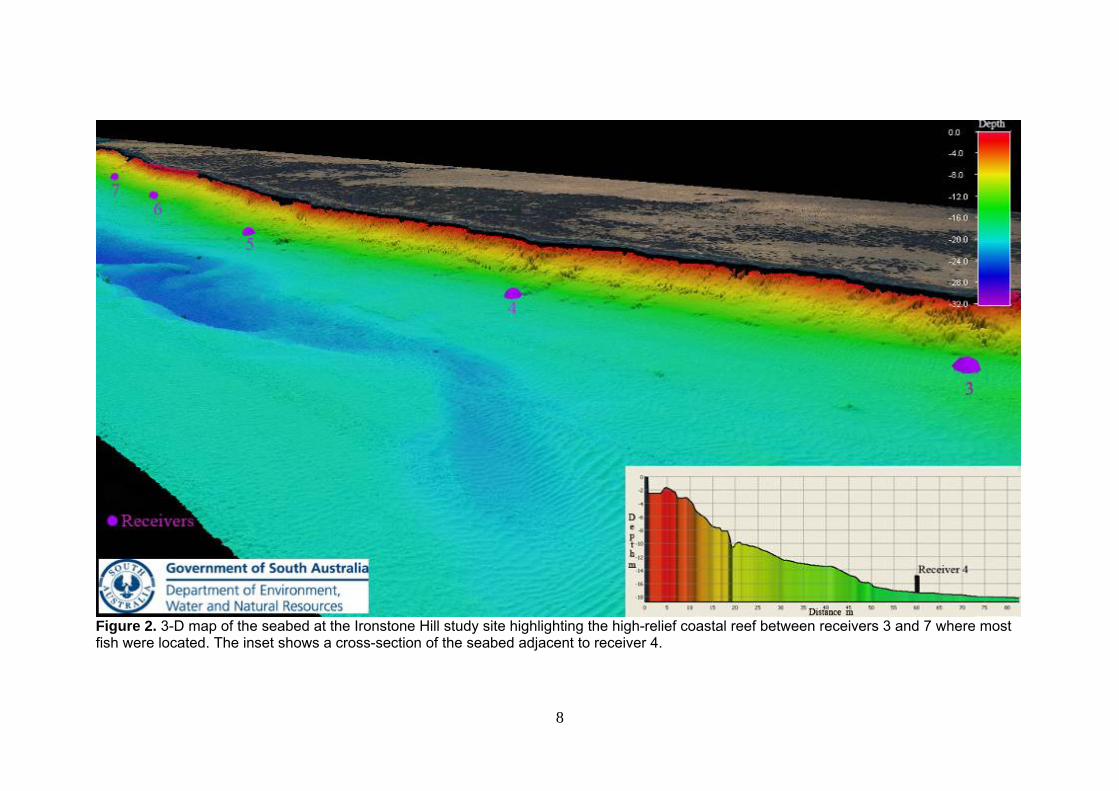
Figure 2. 3-D map of the seabed at the Ironstone Hill study site highlighting the high-relief coastal reef between receivers 3 and 7 where most fish were located. The inset shows a cross-section of the seabed adjacent to receiver 4.

8

Receiver deployment

The VEMCO® acoustic tracking technology requires the receivers to be moored to

the seafloor where they passively detect and log the signals of individual fish that

have been tagged with coded transmitters (Heupel et al. 2006, www.vemco.com).

Receivers are separated by a distance that is a function of the detectable range of

the signal from the transmitters. To inform the appropriate distance between the

receivers in our study, results from range testing and fish detections at a comparable

site in a previous study were used (Bryars et al. 2011, 2012). A nominal spacing

interval of 400 m between receivers was used at the Ironstone Hill site.

Deployment of receivers was undertaken on 9/6/2010. Receivers 2 to 7 were located

~50-100 m offshore from the edge of the coastal reef in 10–19 m depth (Figs. 1, 2).

Receiver 1 had to be located farther offshore (~200 m) due to the shallow

embayment and was set in ~8 m depth. The seven receivers encompassed a total

distance of ~2.4 km. Receivers were affixed with cable ties to 1.65 m long steel posts

that had been hammered into the sand such that receivers were ~1 m above the

seabed and the hydrophone was clear of the top of the post.

Transmitter deployment

Fish were tagged between 7/6/10 and 11/6/10 (Table 1). Fish were captured

underwater by scuba divers at depths of <12 m from along the high-relief reef using a

hand-held dab net. Fish were slowly brought to the surface to reduce the chance of

barotrauma. Each fish was immediately transferred to a plastic tub containing an

oxygen enriched solution of 40 ppm eugenol (AQUI-S, AQUIS-S NZ) for anaesthetic

induction which took 15–20 minutes. A cover was placed on the surface of the tub to

reduce visual stimulation during induction. Once surgical anaesthesia had been

achieved, as judged by lack of a righting reflex and failure to respond to stimuli, the

fish were placed on a padded cradle in dorsal recumbancy. Anaesthesia was

maintained using a recirculating pump system (~10 litres per minute) from an

induction sump tank with the eugenol concentration further diluted to 20 ppm.

Passage of water over and coverage of gill arches was achieved by regulating the

operculum opening and subsequent drainage back into the sump.

The skin was prepared for surgical incision with a light iodine (Betadine®,

Mundipharma B.V., Netherlands) scrub. The removal of a few scales allowed a small

incision (~20 mm length) to be made with a scalpel blade (#10) along the ventral

midline, and continued through the linea alba into the coelom, proximal to the cloaca

9

at about ¼ of the distance from the cloaca to the base of the ventral fins. An antibiotic

soaked (Nuflor® LA, Florfenicol, Schering-Plough Animal Health) transmitter was

inserted directly into the coelomic cavity where it became free-floating. Skin and body

wall closure was undertaken using 1/0 PDS® (polyglactin 910, Ethicon, a

monofilament absorbable suture material) in a simple interrupted suture pattern. Fish

were marked with two external dart tags (Hallprint®, 85 mm long, 2 mm dia.) that

were inserted into the dorsal musculature. External tags were used to eliminate the

risk of re-capturing the same fish and to enable scuba divers to observe the post-

release behaviour of tagged fish. Total body length was measured to the nearest 1

cm and weight was estimated to the nearest 0.5 kg which allowed administration of a

long acting antibiotic intramuscularly (Florfenicol, 30 mg/kg).

Fish were then placed into a recovery bath containing clean seawater that was

regularly flushed and aerated using a deck hose. During recovery the fish were

monitored for a return of reflexes and movement of the opercula, fins, and body in a

coordinated fashion. Once fully recovered after 20–60 min., fish were released at the

seabed by scuba divers at their capture location.

As the detection range and diel pattern of detections can vary depending upon

ambient conditions (Payne et al. 2010), a control transmitter was also deployed on

10/6/2010 to assist with interpretation of receiver detections. The control transmitter

was located approximately mid-way between receivers 3 and 4 where it was attached

by monofilament line to an anchor and a subsurface float such that it was situated ~1

m above the seabed.

Receiver data

Receiver data were downloaded on 19/10/10, 24/01/11, and 6/10/11, when the study

was terminated after 16 months. Receiver 7 could not be located at the final

download and so data are missing from the eastern extreme of the array for the

second half of the study.

Analyses utilised data from the 482 full days of data collection commencing on

11/6/10 when all receivers were in place and all fish had been tagged, and finishing

on 5/10/11 when the final 24-hour period of data collection occurred. While data from

receiver 7 were missing for the last 255 days of the study, results from the previous

227 days indicated that it was unlikely that the receiver would have logged much

detection anyway. Therefore the partial absence of receiver 7 was ignored when

10

conducting any analyses involving the full receiver array and study period. Data were

analysed for site fidelity, home range, alongshore movements, depth utilisation, and

diel activity patterns (see next sections). Data from the control transmitter were used

to inform interpretations about site fidelity, any possible alongshore movements, and

diel activity patterns. Detection efficiency of the control transmitter was calculated as

the total number of detections made at each receiver divided by the total number of

transmissions possible across the 482 days using the nominal delay of 10 minutes

for the transmitter (i.e., 69,408 transmissions).

Site fidelity

Site fidelity or residence time for each fish was calculated by dividing the total

number of days with ≥1 detection in the receiver array by the total number of days

available for detection (482 days). While some studies utilise a cut-off of ≥2

detections per day (e.g. Green and Starr 2011) and VEMCO® recommends caution

with single detections, due to the sedentary and secretive habit of the harlequin fish

and the high level of site fidelity it was felt that single detections mostly represented

real fish detections and were not false detections, i.e. it was highly likely that a fish

was actually present within the array on those days with single detections but that the

fish was either not particularly active, at the detection range limits of the receivers,

and/or the acoustic signals were consistently being shielded by the high-relief reef

structure.

Home range

Home range can be defined as the area used by an individual during normal activities

and is commonly defined as the area in which an individual spends 95% of its time

(Tolimieri et al. 2009). Due to the near-linearity of the receiver array along the coast,

traditional home range techniques such as kernel density estimates could not provide

effective area-based home range estimates. The use of activity centres

(Simpfendorfer et al. 2002) was also inappropriate because the receivers did not

have a significant over-lap of detection ranges (Fig. 1) (e.g. Farmer and Ault 2011).

Instead, as a proxy for activity space we used the linear extent of the coast utilised by

each fish across the entire study period to calculate two different estimates of home

range size: alongshore length of coast, and area of reef (after Bryars et al. 2012).

Home range lengths were calculated as the sum of distances (plus 200 m) between

the receivers that accounted for 95% of all detections. Calculations commenced with

the receiver with the greatest number of detections and then progressed to the

11

adjacent receiver with the next highest total, and so on. The additional 200 m was

added to account for the distance (i.e. 100 m) at which detection frequency begins to

decline significantly (unpublished data). Thus, in the case of a single receiver that

accounted for the entire home range (i.e., 100% of detections), the range would be

200 m. Home range area was calculated by multiplying the range length by the width

of the reef utilised by each individual for 95% of the time. The reef width utilised by

each fish was calculated using the depth range that accounted for 95% of all depth

detections (see Depth utilisation below), a mean reef width of 50 m in the middle part

of the array (between receivers 3 to 5), and a mean depth of 12 m at the reef edge.

As this calculation technique is likely to generate considerable over-estimates of

home range size (see Bryars et al. 2012), calculations were limited to the five fish

with the largest number of detections and values are presented as indicative

maximum values only (see Discussion for further details).

Alongshore movements

Analysis of alongshore movements was conducted by plotting individual receiver

detections against time. Alongshore movements were considered to be real when (1)

a detection(s) was made at >1 receiver distance away from the ‘home base’ receiver

where the majority of detections had been made prior to the new detection and (2)

the detection(s) was not simultaneous with a detection at the home base receiver.

This rule was applied because (1) while in some cases fish appeared to have their

home range close to a single receiver (and all detections occurred at this receiver),

other fish appeared to be based in between two receivers and in these cases

‘normal’ detection patterns involved two adjacent receivers, and (2) detection

distance varied with environmental conditions, as evidenced by the control

transmitter which was occasionally simultaneously detected at much greater

distances than usual (up to 800 m).

Depth utilisation

To examine general patterns of depth utilisation, depth data were binned into 1 m

depth classes and plotted as the percentage of total detections versus depth class.

To examine broad changes in depth utilisation across the study period, raw depth

data for each fish were plotted against time. To examine possible diel changes in

depth utilisation, raw depth data for each fish were plotted against 24-hour time.

These plots revealed some possible trends that were then tested statistically. To

allow for a diel influence on the data (see next section), data were separated into two

7-hour periods of night (9PM–4AM) and day (9AM–4PM) which eliminated

12

crepuscular hours around dawn and dusk (see Green and Starr 2011) and also

allowed for the influence of daily variation in the times of dawn and dusk across a

year. To test for a statistical difference between seasons in depth range, minimum

depth, and maximum depth, data from each fish for winter 2010, summer, and winter

2011 were utilised in separate paired t-tests (i.e. winter 2010 vs. summer, and winter

2011 vs. summer). Mean seasonal values of depth range, minimum depth, and

maximum depth were derived from monthly values for the three relevant months.

Paired t-tests were used here and for other datasets (see later) because of the

dependency of the two variables on one another, i.e., pairs of samples from the two

variables were measured from the same individual fish. Paired t-tests only assume

that the differences between the paired values from each variable (in this case, the

differences between means) come from a normally distributed population of

differences; they do not have the same normality and equality of variance

assumptions of a two-sample t-test (Zar 1984). Given the small numbers of fish

involved (<10) it was felt that formal testing of normality (e.g. a Shapiro-Wilk test) was

futile, but rather it was assumed that each t-test was valid and robust to any minor

deviations from normality.

Diel activity patterns

Payne et al. (2010) demonstrated that caution must be exercised when interpreting

diel activity patterns from acoustic detection data, and we have adopted their

approach in analysing our data for possible diel patterns. Detections for each fish

were summed for each hour of each day throughout the entire array, and mean

detection frequency per hourly bin was then calculated based upon the total number

of days each fish was detected within the array (Table 1). For each fish, these

detection frequencies were then divided by the grand mean detection frequency as

calculated from the 24-hourly bins to get standardised detection frequencies (SDFs)

that correct for the variable magnitude of detection patterns among individuals. Using

data from our single fixed-location control transmitter we employed the approach

developed by Payne et al. (2010) to correct for ambient environmental changes in

detection frequency for each fish by using the control SDFs per hourly bin. Data from

the entire 482 detection days of the control transmitter were used in the correction.

To test for a statistical difference in activity between day and night, control-corrected

SDFs from each fish for midnight (12–1AM bin) and midday (12–1PM bin) were

utilised in a paired t-test.

13

Seasonal activity patterns

Deployment of the control transmitter allowed some unique but limited observations

on potential seasonal changes in detection efficiency (given that just one control

transmitter was used and only one summer and two winters were sampled). Payne et

al. (2010) demonstrated that environmental factors can influence detection efficiency

from tagged animals over diel timescales. The potential influence of seasonal

changes on environmental factors has not been investigated. Nonetheless, it was

evident from the 16-month dataset that the frequency of detections (which might

generally be interpreted as activity, Payne et al. 2010) may have been higher during

summer than winter. As with the diel activity data, such patterns could potentially be

influenced by environmental factors. As a first step in investigating the potential for

this to occur on a seasonal basis, a limited dataset was analysed using a similar

method to the diel data.

For four of the individuals that were present in the array for most of the study period

and which displayed similar and ‘typical’ behaviour patterns, a comparison was made

across all months (except October 2011 for which insufficient data were available)

and between summer (Dec–Feb) and the two winters (Jun–Aug, 2010 and 2011).

Total daily detections from all receivers for each of the four fish and the control

transmitter were used to calculate mean monthly detections separately. SDFs were

then calculated for each month and the fish SDFs were also control-corrected (after

the method of Payne et al. 2010). SDF values were plotted against time (month) to

examine possible trends. Mean summer and winter control-corrected SDFs were

calculated using the monthly mean values from the three relevant months per

season, and a statistical comparison made of summer versus winter 1 (2010) and

summer versus winter 2 (2011) using paired one-tailed t-tests to investigate if activity

(as defined by control-corrected SDF) was greater in summer than winter.

14

Results

Fish capture and size

All fish were captured and released during daylight hours between 7–11/06/11

between receivers 3 and 5 (Table 1). Fish ranged in size from 330 to 620 mm TL and

0.5 to 3 kg weight (Table 1). Based upon maximum length alone (i.e., 760 mm TL,

Hutchins and Swainston 2002), it is possible that all fish except Fish 10 were adult.

Fish sex was not determined as external sexually-diagnostic characters are not

known.

Table 1. Summary of the 10 harlequin fish tagged within the receiver array. First and

last days of detections were nominally 11/06/10 and 5/10/11, respectively. * = a

single detection was later recorded on 31/12/10. Total number days detected =

number of days in which ≥1 detection occurred in a 24-hour period. Residence time =

total number days detected divided by the total number days available for detection

(482 days).

Fish no.

Total length (mm)

Approx. wt (kg)

Release date

Last day detected

Total no. detections

Total no. days

detected

Residence time (%)

1 410 1.0 07/06/10 26/07/11 5696 257 53.3

2 410 1.0 07/06/10 10/07/10* 1422 26 5.4

3 460 1.5 07/06/10 05/10/11 54631 479 99.4

4 570 2.5 07/06/10 05/10/11 7422 421 87.3

5 410 1.0 07/06/10 05/10/11 75185 481 99.8

6 580 2.5 10/06/10 05/10/11 7071 408 84.6

7 570 2.5 10/06/10 05/10/11 37723 468 97.1

8 620 3.0 10/06/10 05/10/11 56628 472 97.9

9 510 2.0 10/06/10 05/10/11 34205 476 98.8

10 330 0.5 11/06/10 15/06/10 713 5 1.0

Natural fish behaviour

It was assumed that the tagging procedure and internal transmitters did not affect the

natural behaviour of the fish during the study period. Fish 7 was observed within the

receiver array whilst diving on 24/01/11 (Fig. 3), seven months post-tagging. It

appeared in good health and was moving about freely.

15

Figure 3. Harlequin Fish 7 with a yellow external dart tag visible towards the rear of

the fish. The presence of an external tag indicates that the fish has an internal

transmitter. Individual fish can also be photo-identified using the arrangement of

spots on the head and gill covers. This fish was photographed within the receiver

array on 24/01/11 in the same location that it was tagged on 10/06/10. Photo: S.

Bryars

General temporal patterns of detection

A total of ~280,000 detections were recorded from the 10 fish during the 16-month

study period (Table 1, Fig. 4). On the final full day available for analyses (5/10/11),

seven of the tagged fish were still being detected within the array (Fish 3 to 9; Fig. 4,

Table 1). Five of these fish (Fish 3, 5, 7, 8 and 9) were detected almost every day

over the 16-month period (Fig. 4, Table 1). In contrast, Fish 10 was detected for just

5 days post-tagging (Fig. 4, Table 1). Fish 2 was detected on most days post-release

up until 10/07/10 but was then not detected for a period of 174 days until a single

detection was recorded on 31/12/10; giving a total of just 26 detection days (Fig. 4).

Fish 1 was detected regularly up until 26/07/11 when detections ceased at 411 days

after the first detection, for a total of 257 detection days (Fig. 4, Table 1). Even for

fish that were still being detected at the end of the study, there was considerable

variation in the total number of detections (Table 1); Fish 3, 5, 7, 8 and 9 had by far

the greatest number of detections (>34,000 each) while Fish 4 and 6 had <8,000

detections each (Table 1). The number of detections was not related to fish length for

16

the seven fish still being detected at the completion of the study (linear regression:

F1,6 = 2.57, P = 0.169).

The control transmitter was detected at least once every day of the study period.

Around 60,000 detections were recorded from the control transmitter with 69% of

these at receiver 3, 30% at receiver 4, and the small remainder (~1%) at receivers 1

and 2 (Fig. 5). Detection efficiency at receivers 3 and 4 (which were ~200 m from the

control transmitter) was 60% and 26%, respectively. These results indicate that at

>200 m from a receiver the chance of a detection is substantially lowered and is

consistent with previous range testing which showed that detection efficiency begins

to decline significantly at >100 m distance (S Bryars, unpublished data).

0

1

2

3

4

5

6

7

8

9

10

Jun‐10

Jul‐10

Aug‐10

Sep‐10

Oct‐10

Nov‐10

Dec‐10

Jan‐11

Feb‐11

Mar‐11

Apr‐11

May‐11

Jun‐11

Jul‐11

Aug‐11

Sep‐11

Oct‐11

Fis

h nu

mb

er

Date (month-year)

Figure 4. Time-series of all daily detections within the receiver array for each of the

10 harlequin fish from June 2010 to October 2011. The control transmitter was

detected every day and is not plotted.

17

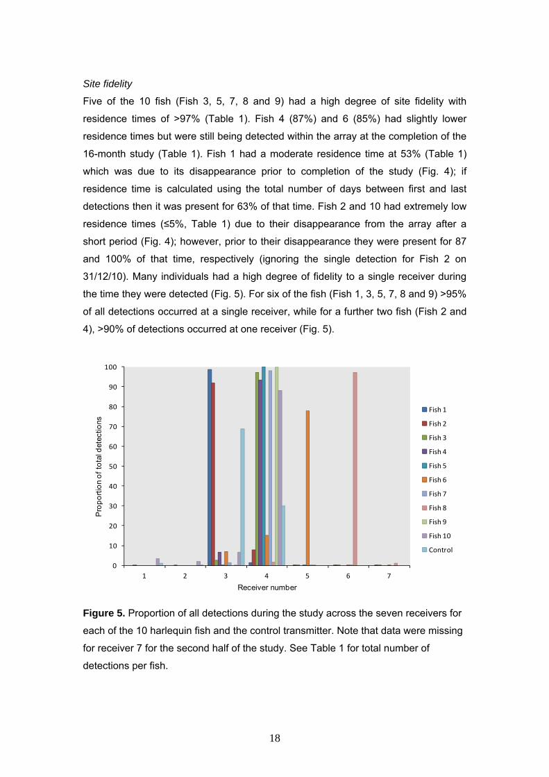
Site fidelity

Five of the 10 fish (Fish 3, 5, 7, 8 and 9) had a high degree of site fidelity with

residence times of >97% (Table 1). Fish 4 (87%) and 6 (85%) had slightly lower

residence times but were still being detected within the array at the completion of the

16-month study (Table 1). Fish 1 had a moderate residence time at 53% (Table 1)

which was due to its disappearance prior to completion of the study (Fig. 4); if

residence time is calculated using the total number of days between first and last

detections then it was present for 63% of that time. Fish 2 and 10 had extremely low

residence times (≤5%, Table 1) due to their disappearance from the array after a

short period (Fig. 4); however, prior to their disappearance they were present for 87

and 100% of that time, respectively (ignoring the single detection for Fish 2 on

31/12/10). Many individuals had a high degree of fidelity to a single receiver during

the time they were detected (Fig. 5). For six of the fish (Fish 1, 3, 5, 7, 8 and 9) >95%

of all detections occurred at a single receiver, while for a further two fish (Fish 2 and

4), >90% of detections occurred at one receiver (Fig. 5).

0

10

20

30

40

50

60

70

80

90

100

1 2 3 4 5 6 7

Pro

po

rtio

n o

f to

tal d

etec

tions

Receiver number

Fish 1

Fish 2

Fish 3

Fish 4

Fish 5

Fish 6

Fish 7

Fish 8

Fish 9

Fish 10

Control

Figure 5. Proportion of all detections during the study across the seven receivers for

each of the 10 harlequin fish and the control transmitter. Note that data were missing

for receiver 7 for the second half of the study. See Table 1 for total number of

detections per fish.

18

Home range

Estimates of home range were made only for the five fish (Fish 3, 5, 7, 8, and 9,

mean TL = 51.4 cm) that had the highest number of detections (all >34,000, with next

highest at ~7,400 for Fish 4) and that remained within the receiver array for almost

the entire 16-month study period (but see Alongshore movements). Each of these

fish had >95% of detections at one receiver and based upon the technique of Bryars

et al. (2012), the home range along-shore length of these fish is a maximum of 200 m

and home range area a maximum of 6,000 m2.

Alongshore movements

Examination of receiver presence-data and depth-data across time revealed that (1)

during July 2010 five of the fish (and possibly more) undertook a short-term but

relatively long-distance coordinated movement along the coast and into deeper

water, (2) at this same time one fish relocated its home range and another fish

permanently left the array, and (3) Fish 10 may have died early in the study.

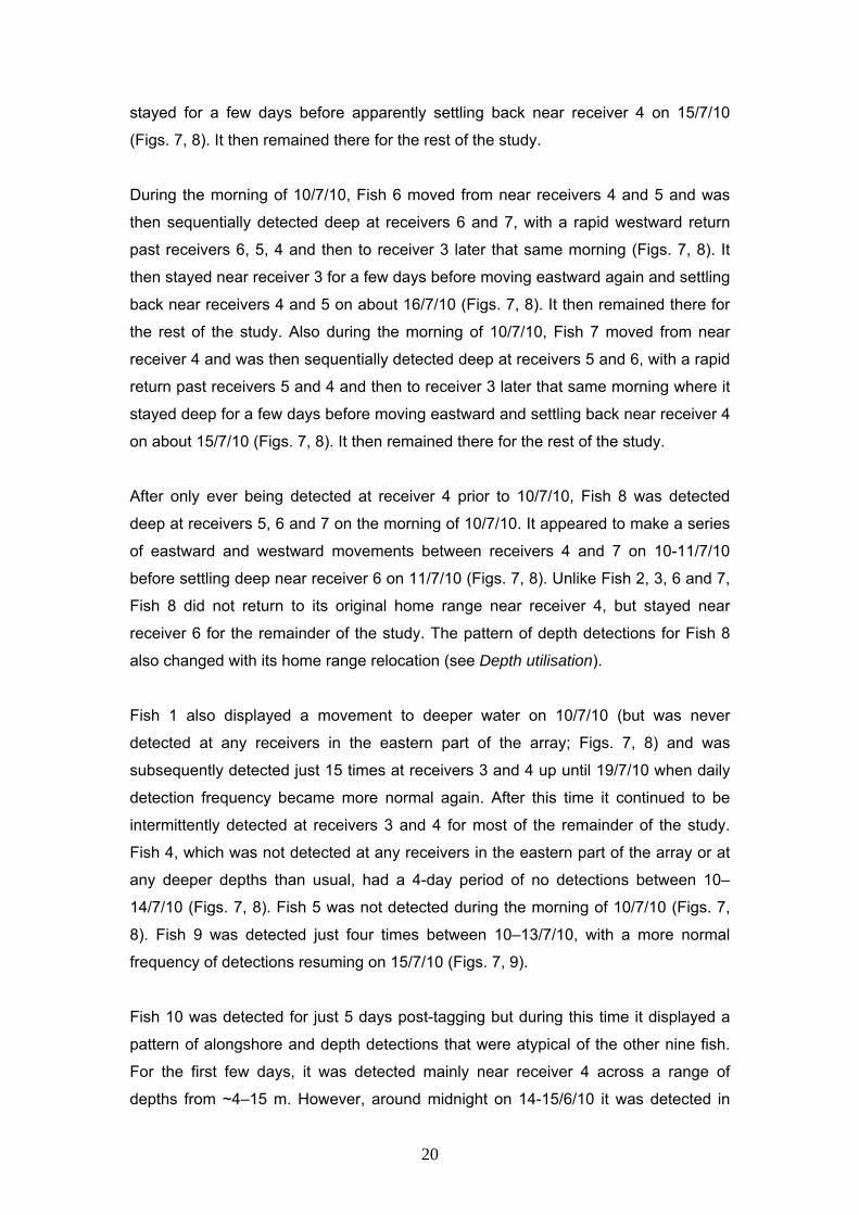
On the morning of 10/7/10, seven of the fish displayed a distinct change in their

pattern of alongshore receiver and/or depth detections (Figs. 7, 8). After previously

only being detected at just one or two receivers within the middle of the array for

about one month post-tagging (usually receivers 3 and 4, or 4 and 5), Fish 2, 3, 6, 7,

and 8 were suddenly detected at receivers 5, 6 and/or 7 in the eastern part of the

array. For each of these fish, the eastward alongshore movement was accompanied

by a movement down the reef slope to depths of ~15–18 m (deeper than any

previously recorded, Fig. 8). The alongshore pattern of detections by these fish was

not replicated by the control transmitter (which was only detected at receivers 1, 3

and 4 during this time period, Fig. 7) and was therefore concluded to be a real

pattern of detections rather than a series of false detections.

After only ever being detected at receivers 3 and 4 prior to 10/7/10, Fish 2 was

sequentially detected deep at receivers 5, 6 and 7 on the morning of 10/7/10 (Figs. 7,

8) and was then not detected throughout the array for the remainder of the study

(except for a single detection at receiver 4 on 31/12/10 which in this particular case

could have been a false detection, Fig. 4). During the morning of 10/7/10, Fish 3

moved from near receiver 4 and was then sequentially detected deep at receivers 5,

6, and 7, with a rapid return to receivers 6 and then 5 later that same day where it

19

stayed for a few days before apparently settling back near receiver 4 on 15/7/10

(Figs. 7, 8). It then remained there for the rest of the study.

During the morning of 10/7/10, Fish 6 moved from near receivers 4 and 5 and was

then sequentially detected deep at receivers 6 and 7, with a rapid westward return

past receivers 6, 5, 4 and then to receiver 3 later that same morning (Figs. 7, 8). It

then stayed near receiver 3 for a few days before moving eastward again and settling

back near receivers 4 and 5 on about 16/7/10 (Figs. 7, 8). It then remained there for

the rest of the study. Also during the morning of 10/7/10, Fish 7 moved from near

receiver 4 and was then sequentially detected deep at receivers 5 and 6, with a rapid

return past receivers 5 and 4 and then to receiver 3 later that same morning where it

stayed deep for a few days before moving eastward and settling back near receiver 4

on about 15/7/10 (Figs. 7, 8). It then remained there for the rest of the study.

After only ever being detected at receiver 4 prior to 10/7/10, Fish 8 was detected

deep at receivers 5, 6 and 7 on the morning of 10/7/10. It appeared to make a series

of eastward and westward movements between receivers 4 and 7 on 10-11/7/10

before settling deep near receiver 6 on 11/7/10 (Figs. 7, 8). Unlike Fish 2, 3, 6 and 7,

Fish 8 did not return to its original home range near receiver 4, but stayed near

receiver 6 for the remainder of the study. The pattern of depth detections for Fish 8

also changed with its home range relocation (see Depth utilisation).

Fish 1 also displayed a movement to deeper water on 10/7/10 (but was never

detected at any receivers in the eastern part of the array; Figs. 7, 8) and was

subsequently detected just 15 times at receivers 3 and 4 up until 19/7/10 when daily

detection frequency became more normal again. After this time it continued to be

intermittently detected at receivers 3 and 4 for most of the remainder of the study.

Fish 4, which was not detected at any receivers in the eastern part of the array or at

any deeper depths than usual, had a 4-day period of no detections between 10–

14/7/10 (Figs. 7, 8). Fish 5 was not detected during the morning of 10/7/10 (Figs. 7,

8). Fish 9 was detected just four times between 10–13/7/10, with a more normal

frequency of detections resuming on 15/7/10 (Figs. 7, 9).

Fish 10 was detected for just 5 days post-tagging but during this time it displayed a

pattern of alongshore and depth detections that were atypical of the other nine fish.

For the first few days, it was detected mainly near receiver 4 across a range of

depths from ~4–15 m. However, around midnight on 14-15/6/10 it was detected in

20

very shallow water (2 m) near receiver 4. The next detection was then made at 16 m

just 17 minutes later at receiver 3. Over the next 2.5 hours there were a series of

detections from receivers 3, then 2 and then 1, indicating a rapid westward

movement, which were accompanied by a series of rapid depth movements ranging

between 0 and 16 m depth. No other fish was ever detected at 0 m depth. The final

detection for Fish 10 was at 3AM in 7 m depth at receiver 1 in the western extreme of

the array.

Diel activity patterns

Diel patterns of activity (as defined by control-corrected SDFs) were similar among

individuals, with the relative frequency of detections increasing dramatically at dawn

and decreasing quickly at dusk (Fig. 9). Some fish did have a higher level of activity

at night than others (e.g. 5 and 8) but the diel pattern was still evident in these fish

(Fig. 9). Mean control-corrected SDF (Fig. 10) was significantly greater at midday

than midnight (Paired two-tailed t-test: t = -9.38, d.f. = 8, P < 0.001).

21

1

2

3

4

5

6

7

8/0

7/1

0

9/0

7/1

0

10

/07

/10

11

/07

/10

12

/07

/10

13

/07

/10

14

/07

/10

15

/07

/10

16

/07

/10

17

/07

/10

18

/07

/10

Rec

eive

r nu

mb

er

Date

Fish 2

1

2

3

4

5

6

7

8/0

7/1

0

9/0

7/1

0

10

/07

/10

11

/07

/10

12

/07

/10

13

/07

/10

14

/07

/10

15

/07

/10

16

/07

/10

17

/07

/10

18

/07

/10

Rec

eive

r nu

mb

erDate

Fish 4

1

2

3

4

5

6

7

8/0

7/1

0

9/0

7/1

0

10

/07

/10

11

/07

/10

12

/07

/10

13

/07

/10

14

/07

/10

15

/07

/10

16

/07

/10

17

/07

/10

18

/07

/10

Rec

eive

r nu

mb

er

Date

Fish 6

1

2

3

4

5

6

7

8/0

7/1

0

9/0

7/1

0

10

/07

/10

11

/07

/10

12

/07

/10

13

/07

/10

14

/07

/10

15

/07

/10

16

/07

/10

17

/07

/10

18

/07

/10

Rec

eive

r nu

mb

er

Date

Fish 8

1

2

3

4

5

6

7

8/0

7/1

0

9/0

7/1

0

10

/07

/10

11

/07

/10

12

/07

/10

13

/07

/10

14

/07

/10

15

/07

/10

16

/07

/10

17

/07

/10

18

/07

/10

Rec

eive

r nu

mb

er

Date

Control

1

2

3

4

5

6

7

8/0

7/1

0

9/0

7/1

0

10

/07

/10

11

/07

/10

12

/07

/10

13

/07

/10

14

/07

/10

15

/07

/10

16

/07

/10

17

/07

/10

18

/07

/10

Rec

eive

r nu

mb

er

Date

Fish 1

1

2

3

4

5

6

7

8/0

7/1

0

9/0

7/1

0

10

/07

/10

11

/07

/10

12

/07

/10

13

/07

/10

14

/07

/10

15

/07

/10

16

/07

/10

17

/07

/10

18

/07

/10

Rec

eive

r nu

mb

er

Date

Fish 3

1

2

3

4

5

6

7

8/0

7/1

0

9/0

7/1

0

10

/07

/10

11

/07

/10

12

/07

/10

13

/07

/10

14

/07

/10

15

/07

/10

16

/07

/10

17

/07

/10

18

/07

/10

Rec

eive

r nu

mb

er

Date

Fish 5

1

2

3

4

5

6

7

8/0

7/1

0

9/0

7/1

0

10

/07

/10

11

/07

/10

12

/07

/10

13

/07

/10

14

/07

/10

15

/07

/10

16

/07

/10

17

/07

/10

18

/07

/10

Rec

eive

r nu

mb

er

Date

Fish 7

1

2

3

4

5

6

7

8/0

7/1

0

9/0

7/1

0

10

/07

/10

11

/07

/10

12

/07

/10

13

/07

/10

14

/07

/10

15

/07

/10

16

/07

/10

17

/07

/10

18

/07

/10

Rec

eive

r nu

mb

er

Date

Fish 9

Figure 7. Receiver detections against time for the 10-day period between 8/7/10 and

18/7/10 for harlequin Fish 1 to 9 and the control transmitter.

22

02468

101214161820

8/0

7/1

0

9/0

7/1

0

10

/07

/10

11

/07

/10

12

/07

/10

13

/07

/10

14

/07

/10

15

/07

/10

16

/07

/10

17

/07

/10

18

/07

/10

Dep

th (m

)

Date

Fish 2

02468

101214161820

8/0

7/1

0

9/0

7/1

0

10

/07

/10

11

/07

/10

12

/07

/10

13

/07

/10

14

/07

/10

15

/07

/10

16

/07

/10

17

/07

/10

18

/07

/10

Dep

th (m

)

Date

Fish 4

02468

101214161820

8/0

7/1

0

9/0

7/1

0

10

/07

/10

11

/07

/10

12

/07

/10

13

/07

/10

14

/07

/10

15

/07

/10

16

/07

/10

17

/07

/10

18

/07

/10

Dep

th (m

)

Date

Fish 6

02468

101214161820

8/0

7/1

0

9/0

7/1

0

10

/07

/10

11

/07

/10

12

/07

/10

13

/07

/10

14

/07

/10

15

/07

/10

16

/07

/10

17

/07

/10

18

/07

/10

Dep

th (m

)

Date

Fish 8

02468

101214161820

8/0

7/1

0

9/0

7/1

0

10

/07

/10

11

/07

/10

12

/07

/10

13

/07

/10

14

/07

/10

15

/07

/10

16

/07

/10

17

/07

/10

18

/07

/10

Dep

th (m

)

Date

Fish 1

02468

101214161820

8/0

7/1

0

9/0

7/1

0

10

/07

/10

11

/07

/10

12

/07

/10

13

/07

/10

14

/07

/10

15

/07

/10

16

/07

/10

17

/07

/10

18

/07

/10

Dep

th (m

)

Date

Fish 3

02468

101214161820

8/0

7/1

0

9/0

7/1

0

10

/07

/10

11

/07

/10

12

/07

/10

13

/07

/10

14

/07

/10

15

/07

/10

16

/07

/10

17

/07

/10

18

/07

/10

Dep

th (m

)

Date

Fish 5

02468

101214161820

8/0

7/1

0

9/0

7/1

0

10

/07

/10

11

/07

/10

12

/07

/10

13

/07

/10

14

/07

/10

15

/07

/10

16

/07

/10

17

/07

/10

18

/07

/10

Dep

th (m

)

Date

Fish 7

02468

101214161820

8/0

7/1

0

9/0

7/1

0

10

/07

/10

11

/07

/10

12

/07

/10

13

/07

/10

14

/07

/10

15

/07

/10

16

/07

/10

17

/07

/10

18

/07

/10

Dep

th (m

)

Date

Fish 9

Figure 8. Depth detections against time for the 10-day period between 8/7/10 and

18/7/10 for harlequin Fish 1 to 9.

23

0

0.5

1

1.5

2

2.5

3

0 2 4 6 8 10 12 14 16 18 20 22

Sta

ndar

dis

ed d

etec

tion

freq

uenc

y

Hourly bin

1

2

3

4

5

6

7

8

9

Figure 9. Diel activity patterns of individual fish: control-corrected standardised

detection frequencies per hourly bin for individual harlequin Fish 1 to 9.

0

0.5

1

1.5

2

0 1 2 3 4 5 6 7 8 9 10 11 12 13 14 15 16 17 18 19 20 21 22 23

Sta

nd

ard

ised

det

ect

ion

freq

uenc

y

Hourly bin

Figure 10. Diel activity pattern for all fish combined: mean (± SE) control-corrected

standardised detection frequency per hourly bin for harlequin Fish 1 to 9.

24

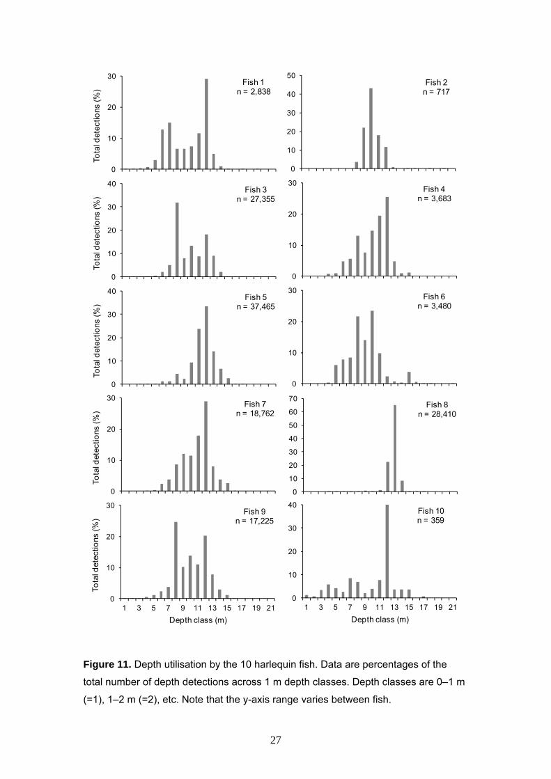
Depth utilisation

Individual fish utilised a range of depths but depth utilisation was non-uniform (Fig.

11). Some fish had a uni-modal distribution of detections (Fish 2, 5, 7 and 8), while

others had a bi-modal distribution (1, 3, 4, 6, and 9; Fig. 11). The depth distribution of

Fish 10 was influenced by a low number of detections and the unusual behaviour

described earlier, and must therefore be considered as atypical. All fish had relatively

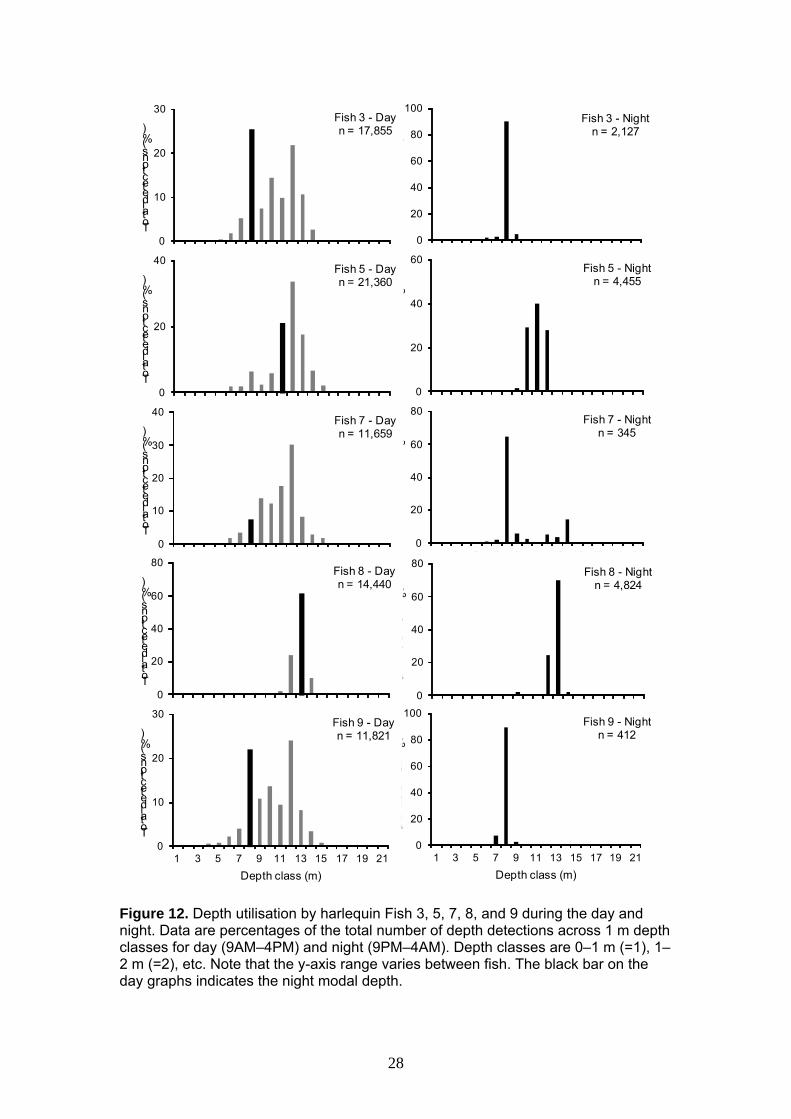
little activity at depths >13 m which is at or near the reef edge (see Fig. 2). For those

fish that had a moderate number of night detections (viz. 3, 5, 7, 8, and 9), patterns

of depth utilisation varied noticeably between day and night (Fig. 12). During the day

a wide range of depths were utilised, while at night a very restricted range was

detected; except for Fish 8 which utilised a small range at all times (Fig. 12). For Fish

7 in which there were a few detections at deeper depths during the night (Fig. 12),

these were all during the period 10-17/7/10 when the fish underwent an unusual

alongshore movement into deeper waters and were thus not representative of the

rest of the study period (see Alongshore movements earlier). Using the coefficient of

variation as a standardised measure of dispersion for Fish 3, 5, 7 (minus the period

10-17/7/10) and 9, the apparent difference between day and night depth distribution

was found to be statistically significant (Paired t-test: t = 6.60, d.f. = 3, P < 0.01). For

each of those fish (Fish 3, 5, 7, and 9), the night modal depth did not correspond with

the day modal depth and was shallower than the day modal depth (Fig. 12); this

suggests that during the daytime these fish were moving from their night home base

down the reef slope into deeper water and then returning to their base at night.

Further evidence that fish exhibited diurnal behaviours was observed in the depth

data which showed a much narrower band of depth utilisation during the night

compared to during the daylight hours (Fig. 12 and Fig. 13 showing Fish 9 which is

typical of many of the fish). A narrow band of night-time depth detections (e.g., ~2 m

amplitude for Fish 9) is likely due mainly to natural tidal fluctuations of ~1.5 m range

and the accuracy of the transmitters (±2.5 m), rather than fish actually moving

vertically across the reef slope at night. Indeed it is most likely that many of the

detections at night were actually due to fish being stationed within caves or ledges

that had a direct ‘line-of-sound’ to nearby receivers. For example, after relocating its

home range, Fish 8 appeared to be based mainly at the reef edge in ~12–13 m (see

below). In such locations, there is a much higher chance of detections from fish lying

inside caves or ledges that are facing seaward and thus towards receivers.

25

Most fish (Fish 1, 3–7, and 9) displayed frequent movements up and down the reef

slope during the daytime with some excursions away from the reef edge which lies in

~12–14 m depth (e.g. Fish 9 in Fig. 14 which is typical of most of the fish). The

pattern of first detections for each day indicated that the fish were utilising a small

number of home bases at set depths during the night before emerging for the first

time each morning. For example, Fish 9 appeared to have a base at ~10–11 m depth

and another at ~7–8 m depth (Fig. 14); the 7–8 m depth class aligns with the peak in

overall activity (Fig. 11, Fish 9) and also the depth at which most night-time

detections occurred (Fig. 13). The patterns of depth detections also indicated that

fish were remaining at set depths for periods of up to several hours during the

daytime.

Seasonal patterns of depth utilisation were different for each fish (Fish 2 and 10 had

too few detections across the entire study period to warrant an examination of

seasonal depth movements). Nonetheless, some consistent patterns were apparent

(except for Fish 8—see below) in which there appeared to be less utilisation of

shallow and deep waters during the winter months (e.g. Fish 9 in Fig. 15). Indeed,

day-time mean depth range was significantly greater in summer (Dec–Feb) than

winter (Jun–Aug) (Paired t-test, winter 1 vs summer: t = -2.77, d.f. = 6, P < 0.05;

Paired t-test, winter 2 versus summer: t = -2.68, d.f. = 6, P < 0.05), and day-time

mean minimum depth was significantly lower in summer than winter (Paired t-test,

winter 1 vs summer: t = 4.25, d.f. = 6, P < 0.01; Paired t-test, winter 2 versus

summer: t = 2.61, d.f. = 6, P < 0.05).

Fish 8 had a markedly different seasonal and daily pattern of depth detections to Fish

1, 3–7 and 9 (Fig. 15). During the first month it showed typical daily depth utilisation

of the reef slope, but following its home range relocation in July 2010 (see

Alongshore movements earlier), it then had very limited depth utilisation for the

remainder of the study (Fig. 15). Apart from a slight change during January 2011, it

mainly utilised 12–13 m depths (Fig. 15), which was clearly the mode for the depth

distribution (Fig. 11) and is at the edge of the reef. Fish 8 had a much higher rate of

detection at night than most other fish (Fig. 9) and this is possibly due to its location

at the reef edge and a more direct ‘line-of-sound’ during the night to the closest

receiver (i.e., receiver 6, Fig. 5).

26

0

10

20

30

40

50

1 3 5 7 9 11 13 15 17 19 21

Tota

l det

ectio

ns (%

)

Depth class (m)

Fish 2n = 717

0

10

20

30

1 3 5 7 9 11 13 15 17 19 21To

tal d

etec

tions

(%)

Depth class (m)

Fish 4n = 3,683

0

10

20

30

1 3 5 7 9 11 13 15 17 19 21

Tota

l det

ectio

ns (%

)

Depth class (m)

Fish 6n = 3,480

0

10

20

30

40

50

60

70

1 3 5 7 9 11 13 15 17 19 21

Tota

l det

ectio

ns (%

)

Depth class (m)

Fish 8n = 28,410

0

10

20

30

40

1 3 5 7 9 11 13 15 17 19 21

Tota

l det

ectio

ns (%

)

Depth class (m)

Fish 10n = 359

0

10

20

30

1 3 5 7 9 11 13 15 17 19 21

Tota

l det

ectio

ns (%

)

Depth class (m)

Fish 1n = 2,838

0

10

20

30

40

1 3 5 7 9 11 13 15 17 19 21

Tota

l det

ectio

ns (%

)

Depth class (m)

Fish 3n = 27,355

0

10

20

30

40

1 3 5 7 9 11 13 15 17 19 21

Tota

l det

ectio

ns (%

)

Depth class (m)

Fish 5n = 37,465

0

10

20

30

1 3 5 7 9 11 13 15 17 19 21

Tota

l det

ectio

ns (%

)

Depth class (m)

Fish 7n = 18,762

0

10

20

30

1 3 5 7 9 11 13 15 17 19 21

Tota

l det

ectio

ns (%

)

Depth class (m)

Fish 9n = 17,225

Figure 11. Depth utilisation by the 10 harlequin fish. Data are percentages of the

total number of depth detections across 1 m depth classes. Depth classes are 0–1 m

(=1), 1–2 m (=2), etc. Note that the y-axis range varies between fish.

27

0

20

40

60

80

100

1 3 5 7 9 11 13 15 17 19 21

Total detections (%)

Depth class (m)

Fish 3 - Nightn = 2,127

0

20

40

60

1 3 5 7 9 11 13 15 17 19 21

Total detections (%)

Depth class (m)

Fish 5 - Nightn = 4,455

0

20

40

60

80

1 3 5 7 9 11 13 15 17 19 21

Total detections (%)

Depth class (m)

Fish 7 - Nightn = 345

0

20

40

60

80

1 3 5 7 9 11 13 15 17 19 21

Total detections (%)

Depth class (m)

Fish 8 - Nightn = 4,824

0

20

40

60

80

100

1 3 5 7 9 11 13 15 17 19 21

Total detections (%)

Depth class (m)

Fish 9 - Nightn = 412

0

10

20

30

1 3 5 7 9 11 13 15 17 19 21

Total detections (%)

Depth class (m)

Fish 3 - Dayn = 17,855

0

20

40

1 3 5 7 9 11 13 15 17 19 21

Total detections (%)

Depth class (m)

Fish 5 - Dayn = 21,360

0

10

20

30

40

1 3 5 7 9 11 13 15 17 19 21

Total detections (%)

Depth class (m)

Fish 7 - Dayn = 11,659

0

20

40

60

80

1 3 5 7 9 11 13 15 17 19 21

Total detections (%)

Depth class (m)

Fish 8 - Dayn = 14,440

0

10

20

30

1 3 5 7 9 11 13 15 17 19 21

Total detections (%)

Depth class (m)

Fish 9 - Dayn = 11,821

Figure 12. Depth utilisation by harlequin Fish 3, 5, 7, 8, and 9 during the day and night. Data are percentages of the total number of depth detections across 1 m depth classes for day (9AM–4PM) and night (9PM–4AM). Depth classes are 0–1 m (=1), 1–2 m (=2), etc. Note that the y-axis range varies between fish. The black bar on the day graphs indicates the night modal depth.

28

0

2

4

6

8

10

12

14

16

18

2012 AM 6 AM 12 PM 6 PM 12 AM

Dep

th (m

)

Time (24 hour)

Figure 13. Diel pattern of depth detections for harlequin Fish 9. Data are depth

detections against 24-hour time for the entire study period.

0

2

4

6

8

10

12

14

16

18

2001 02 03 04 05 06 07 08 09 10 11 12 13 14 15 16 17 18 19 20 21 22 23 24 25 26 27 28 29 30 31 01

Dep

th (m

)

Day of January 2011

Figure 14. Daily pattern of depth detections during January 2011 for harlequin Fish

9. Red points indicate the depth of the first detection for each day.

29

0

2

4

6

8

10

12

14

16

18

20

06

/10

07

/10

08

/10

09

/10

10

/10

11

/10

12

/10

01

/11

02

/11

03

/11

04

/11

05

/11

06

/11

07

/11

08

/11

09

/11

10

/11

Dep

th (m

)

Date (month/year)

0

2

4

6

8

10

12

14

16

18

20

06

/10

07

/10

08

/10

09

/10

10

/10

11

/10

12

/10

01

/11

02

/11

03

/11

04

/11

05

/11

06

/11

07

/11

08

/11

09

/11

10

/11

Dep

th (m

)

Date (month/year)

Figure 15. Seasonal pattern of depth detections for harlequin Fish 9 (upper panel)

and 8 (lower panel). The pattern for Fish 9 was more typical of the rest of the fish in

the study (Fish 1 and 3–7).

30

Seasonal activity patterns

Monthly SDFs for the four harlequin fish that were present within the array for almost

100% of the time and which displayed a typical pattern of depth detections (i.e. Fish

3, 5, 7 and 9), showed some evidence of a seasonal activity pattern (Fig. 16).

However, it appeared that there may also have been some seasonal environmental

effect as monthly SDFs for the control transmitter showed a strong seasonal pattern

with much lower values during the summer than the two winters (Fig. 17). Indeed,

when the fish SDFs were corrected with the control SDFs there was a very strong

pattern of seasonal activity (as defined by control-corrected SDFs) (Fig. 18), with

significantly greater activity in summer (Dec–Feb) than winter 2011 (Jun–Aug) but

not for summer vs. winter 2010 (Paired t-test, winter 2010 vs summer: t = -2.48, d.f. =

3, P = 0.089; Paired t-test, winter 2011 versus summer: t = 3.56, d.f. = 3, P < 0.05).

However, as only one control transmitter was used and only one summer was

available for comparison, the outcomes of the seasonal analysis must be treated with

caution.

0

0.2

0.4

0.6

0.8

1

1.2

1.4

1.6

1.8

Sta

ndar

dis

ed d

etec

tion

freq

uenc

y

Month (2010-2011)

Figure 16. Mean (± SE) standardised detection frequency per month for harlequin

Fish 3, 5, 7 and 9 across the study period.

31

0

0.2

0.4

0.6

0.8

1

1.2

1.4

1.6

Sta

ndar

dis

ed d

etec

tion

freq

uenc

y

Month (2010-2011)

Figure 17. Standardised detection frequency for the control transmitter per month.

0

0.5

1

1.5

2

2.5

Sta

ndar

dis

ed d

etec

tion

freq

uenc

y

Month (2010-2011)

Figure 18. Seasonal activity pattern: mean (± SE) control-corrected standardised

detection frequency per month for harlequin Fish 3, 5, 7 and 9.

32

Discussion

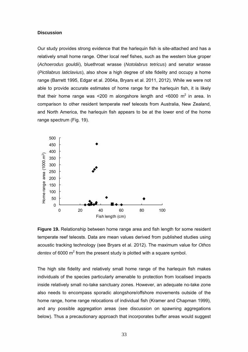
Our study provides strong evidence that the harlequin fish is site-attached and has a

relatively small home range. Other local reef fishes, such as the western blue groper

(Achoerodus gouldii), bluethroat wrasse (Notolabrus tetricus) and senator wrasse

(Pictilabrus laticlavius), also show a high degree of site fidelity and occupy a home

range (Barrett 1995, Edgar et al. 2004a, Bryars et al. 2011, 2012). While we were not

able to provide accurate estimates of home range for the harlequin fish, it is likely

that their home range was <200 m alongshore length and <6000 m2 in area. In

comparison to other resident temperate reef teleosts from Australia, New Zealand,

and North America, the harlequin fish appears to be at the lower end of the home

range spectrum (Fig. 19).

0

50

100

150

200

250

300

350

400

450

500

0 20 40 60 80 10

Ho

me

rang

e ar

ea (

1000

.m2)

Fish length (cm)

0

Figure 19. Relationship between home range area and fish length for some resident

temperate reef teleosts. Data are mean values derived from published studies using

acoustic tracking technology (see Bryars et al. 2012). The maximum value for Othos

dentex of 6000 m2 from the present study is plotted with a square symbol.

The high site fidelity and relatively small home range of the harlequin fish makes

individuals of the species particularly amenable to protection from localised impacts

inside relatively small no-take sanctuary zones. However, an adequate no-take zone

also needs to encompass sporadic alongshore/offshore movements outside of the

home range, home range relocations of individual fish (Kramer and Chapman 1999),

and any possible aggregation areas (see discussion on spawning aggregations

below). Thus a precautionary approach that incorporates buffer areas would suggest

33

that a sanctuary zone of several km in alongshore length and width is required to fully

encompass a population of harlequin fish at locations such as the Ironstone Hill study

site.

Our results indicate that the harlequin fish is a diurnal predator. Other evidence that

harlequin fish are diurnal comes from the Baited Remote Underwater Video System

(BRUVS) work of Kendrick et al. (2005) in which harlequin fish were only ever

recorded during the day-time. Many other serranids are also diurnal (DeLoach and

Humann 1999), as are some other local reef fishes such as the western blue groper

(Achoerodus gouldii) and bluethroat wrasse (Notolabrus tetricus) (Bryars et al. 2011).

As harlequin fish do not move greater than a few metres above the seabed into the

water column, our depth data can be interpreted as fish position on the seabed. Thus

it is apparent that during the day-time individual fish actively moved up and down the

reef slope. These movements were punctuated by periods where their depth did not

change and therefore fish were likely stationary. Such a pattern is consistent with

field observations in which fish regularly rest on the seabed. It is also likely that these

fish were spending some of this time at ambush stations or cleaning stations. The

former behaviour has been observed in the field (S Bryars, pers. obs.) and the latter

behaviour has been documented in harlequin fish (Shepherd et al. 2005, Bryars

2011). In addition, multiple resights of the same individual harlequin fish across many

months have occurred at exactly the same reef ledge (Bryars 2011). In the present

study, most fish had one or more distinct depth modes of activity (Fig. 11) and it is

possible that these were related to ambush/cleaning stations and/or home bases.

Diel depth data indicated that following the day-time period of activity, individuals

were returning to a home base with a set depth each night and that movements away

from this depth at night were limited. Observations of fish in the field show that they

utilise caves or ledges when threatened by divers (S Bryars, pers. obs.), and it is

likely that they utilise these same habitats at night for resting and protection from

predators. The reduced frequency of detections by receivers at night could also be

partly explained by such behaviour as solid structures will impede acoustic signals.

The pattern is consistent with a species that has a small home range for diurnal

activities and a nocturnal home base(s). Such a pattern has been seen in some other

temperate reef fish such as the California sheephead (Semicossyphus pulcher)

(Topping et al. 2005). Further investigation to confirm the 2-D fine-scale movements

of harlequin fish could be undertaken using a VRAP or VPS acoustic telemetry

system (e.g. Jorgensen et al. 2006, Espinoza et al. 2011). It appears that the long-

34

term movement patterns of the harlequin fish are quite different to the coral trout

(Plectropomus leopardus) which is a similarly-sized and shaped member of the

Serranidae family (but which is found in the tropics). The coral trout appears to range

over several kilometres of reefs as a mobile, opportunistic predator, but also

maintains home sites for access to shelter and cleaning stations (Samoilys 1997a). In

contrast, the harlequin fish we studied did not roam over such distances.

Our study provided evidence that harlequin fish had more vertical movement across

the reef slope during summer than winter, with some evidence that they were also

more active during summer. The seasonal activity pattern (based upon control-

corrected SDFs) is closely aligned with the seasonal temperature pattern for the

region. If the seasonal activity pattern is indeed real, then it is possibly due to a direct

relationship between metabolic rate and temperature in teleost fish (Clarke and

Johnston 1999) such that the harlequin fish needed to feed more frequently during

the summer months. In addition, there are more daylight hours for diurnal activity

during summer than in winter such that a greater number of detections might be

expected then anyway.

Given the complexity of the reef system and the sedentary habit of the harlequin fish,

the high number of detections for some fish was somewhat surprising to us. In

contrast, some individuals had a much lower number of detections. Reasons for this

discrepancy could be related to real differences in activity levels and/or differences in

the fine-scale locations of individual fish within the reef complex (and thus differences

in distance and ‘line-of-sound’ to the closest receiver). Nonetheless, our results show

that the type of technology used can be employed successfully on sedentary species

such as harlequin fish in high-relief reef habitats to investigate long-term site fidelity.

Our results also demonstrate the usefulness of long-term tracking data for site-

attached reef fish, as other methods such as visual tagging and tracking (e.g. Barrett

1995, Edgar et al. 2004a), may have missed the alongshore movement that we

detected during July 2010.

The temporary alongshore movement of harlequin fish may have been triggered by

an unusual storm event. Storm activity has been correlated with the onset of

coordinated movement in other site-attached reef fish such as the black rockfish

(Sebastes melanops) (Green and Starr 2011). The maximum wind speed measured

on 10/7/2010 was a direct northerly of 126 km/h, which was the strongest wind speed

recorded from any direction (including from the SW where most major storms blow)

35

throughout all of 2010 and 2011 at nearby Cape Willoughby. The maximum speed of

126 km/h was also far greater than the mean wind speed of 27 km/h recorded for

Cape Willoughby during the study period (Bureau of Meteorology data). As the wind

was directly from the north, the fetch over which waves could be generated was

close to the maximum possible for the Ironstone Hill site at ~145 km (see Fig. 1).

Strong northerly winds can cause a great deal of wave energy along the northern

coastline of Kangaroo Island (S. Bryars pers. obs.) and the extreme northerly winds

on 10/7/2010 would have resulted in greatly increased wave energy in the shallow

waters of the north-facing Ironstone Hill study site (see Fig. 2). It appears that the

wave energy was sufficiently strong to cause fish to flee the shallower coastal waters

and seek shelter in deeper waters offshore (Fig. 2) and further along the coast. All of

the fish that moved alongshore initially moved eastwards; water depths immediately

offshore from the coastal reef are substantially greater in the eastern part of the study

array (>20 m depth; Fig. 2) than to the west (<10 m depth). Another possible

explanation for the alongshore movement was a spawning aggregation. Spawning

aggregations do occur in some serranids (DeLoach and Humann 1999) including the

coral trout (Plectropomus leopardus) which aggregates around new moon periods

(Samoilys 1997b). However, in our study the onset of the movement was not

correlated with a new or full moon, and it occurred in mid-winter which is unlikely to

be a spawning time for local fish species; spawning in many other local fishes is

usually related to a seasonal temperature change or during the warmer summer

months.

Of particular interest in our study was that, while most fish were able to return to their

home range following the storm event, one fish apparently relocated its home range

outside of the study array, and another fish relocated its home range within the array.

Other site-attached fishes have been shown to be able to return to their home ranges

when displaced to a different location (e.g. Lowry and Suthers 1998, Jadot et al.

2006). However, it appears that both the distance of displacement and weather

conditions can influence the ability to successfully return (Lowry and Suthers 1998,

Jadot et al. 2006). In our study it was apparent that following the disturbance of the

storm event, fish that had left their home base then actively searched up and down

the coast for their home base and in some cases this took several days or more to

achieve. However, it appears that two of the fish were not able to find their original

home base and relocated to a suitable (or better) home base elsewhere. Such

relocations reinforce the need for having adequately-sized no-take sanctuary zones

(see Kramer and Chapman 1999).

36

Our behavioural results have implications for the design and interpretation of fish

surveys involving harlequin fish, which are usually relatively rare in fish surveys

(Shepherd and Baker 2008, Bryars 2011). As harlequin fish are diurnal they are

clearly amenable to daytime underwater visual census (UVC) and BRUVS

techniques. As UVC transect lines are traditionally laid parallel to the shoreline at set

depths (e.g. Barrett et al. 2007, Currie and Sorokin 2009), it is apparent that at our

site there would be a much greater chance of encountering adult harlequin fish at

certain depths, thus affecting the chance of detection. In addition, harlequin fish

activity varied across different days (and possibly seasons) and thus the timing of

surveys may also influence the chance of encountering harlequin fish. UVC is known

to have certain biases (Edgar et al. 2004b) and the information from the current study

could potentially assist with the interpretation of UVC data on harlequin fish.

One of the harlequin fish (Fish 10) displayed a particularly unusual pattern of depth

utilisation and alongshore movement before it disappeared just five days post-

tagging. As Fish 10 moved right to the surface at one stage and moved out of the

acoustic array at an extremely rapid rate, it is possible that it was captured by a fast-

moving, air-breathing predator. However, it is unknown whether it suffered

complications post-surgery and that this contributed to its apparent demise, i.e. it was

sick or dead at the time of apparent removal from the array. Fish 10 was the smallest

of the fish tagged at 330 cm TL and ~0.5 kg weight. While the size of the transmitter

was 1.2% of its body weight and this did not break the 2% tag-to-body mass rule

(Childs et al. 2011), we did experience some difficulty with inserting the transmitter

into Fish 10.

In summary, we conclude that the harlequin fish is a site-attached, diurnal predator,

with a relatively small home range. These characteristics, which had not been

demonstrated prior to our study, make individuals of the species amenable to long-

term day-time monitoring techniques and to protection from localised impacts inside

adequately-sized and appropriately-located no-take sanctuary zones. The inclusion

of high-relief reef with caves and ledges in areas where harlequin fish are found is

critical for protection of this particular species.

37

References

Baker, J.L. (2012) Marine Species of Conservation Concern in South Australia:

Volume 1 - Bony and Cartilaginous Fishes. Report for the South Australian Working

Group for Marine Species of Conservation Concern. J. Baker (consultant); Science

and Conservation Division, and Coast and Marine Conservation branches of S.A.

Department for Environment and Heritage (DEH); Marine and Coastal Community

Network of S.A. (MCCN), and Threatened Species Network (TSN). Web version

published by Reef Watch, South Australia.

(http://www.reefwatch.asn.au/pages/bin/view/Publications/SamsccHome).

Barrett, N.S. (1995) Short- and long-term movement patterns of six temperate reef

fishes (Families Labridae and Monacanthidae). Marine and Freshwater Research,

46: 853–860.

Barrett, N.S., Edgar, G.J., Buxton, C.D. and Haddon, M. (2007) Changes in fish

assemblages following 10 years of protection in Tasmanian marine protected areas.

Journal of Experimental Marine Biology and Ecology, 345: 141–157.

Bryars, S. (2011) Monitoring marine fishes of conservation concern on Adelaide’s

coastal reefs: combined results of 2009/2010 and 2010/2011 surveys for the

southern blue devil and harlequin fish. Report to the Adelaide and Mount Lofty

Ranges Natural Resources Management Board. Department of Environment and

Natural Resources. 40 pp.

Bryars, S., Rogers, P., Huveneers, C., Payne, N. Smith, I., and McDonald, B. (2011)

What size do marine park sanctuary zones need to be to protect the Western Blue

Groper Achoerodus gouldii, Harlequin Fish Othos dentex, and Bluethroat Wrasse

Notolabrus tetricus? Final report to the Department of Environment and Natural

Resources Wildlife Conservation Fund Project Number 0638. Department of

Environment and Natural Resources. 36 pp.

Bryars, S., Rogers, P., Huveneers, C., Payne, N., Smith, I., and McDonald, B. (2012)

Small home range in southern Australia’s largest resident reef fish, the western blue

groper (Achoerodus gouldii): implications for adequacy of no-take marine protected

areas. Marine and Freshwater Research 63: 552–563.

38

Bye, J.A.T., and Kämpf, J. (2008) Physical oceanography. In: S.A. Shepherd, S.

Bryars, I. Kirkegaard, P. Harbison, and J.T. Jennings (eds.) ‘Natural History of Gulf St

Vincent’. pp 56–70.

Childs, A.R., Næsje, T.F. and Cowley, P.D. (2011) Long-term effects of different-

sized implanted acoustic transmitters on the sciaenid Arygyrosomus japonicus:

breaking the 2% tag-to-body mass rule. Marine and Freshwater Research, 62: 243–

438.

Clarke, A. and Johnston, N.M. (1999) Scaling of metabolic rate with body mass and

temperature in teleost fish. Journal of Animal Ecology, 68: 893–905.

Currie, D.R. and Sorokin, S.J. (2009) Evaluating the effects of reserve closure on

algae, invertebrate and fish assemblages at a temperate South Australian marine

reserve. Journal of the Marine Biological Association of the United Kingdom, 89(4):

651–661.

DeLoach, N. and Humann, P. (1999) Reef Fish Behaviour: Florida, Caribbean,

Bahamas. New World Publications, Florida.

Department of Environment and Natural Resources (2010) Environmental, Economic

and Social Values of the Encounter Marine Park. Department of Environment and

Natural Resources, South Australia

Edgar, G.J. (2008) Australian Marine Life. The plants and animals of temperate

waters. Reed New Holland, Sydney.

Edgar, G.J., Barrett, N.S. and Morton, A.J. (2004a) Patterns of fish movement on

eastern Tasmanian rocky reefs. Environmental Biology of Fishes, 70: 273–284.

Edgar, G.J., Barrett, N.S. and Morton, A.J. (2004b) Biases associated with the use of

underwater visual census techniques to quantify the density and size-structure of fish

populations. Journal of Experimental Marine Biology and Ecology, 308: 269–290.

Espinoza, M., Farrugia, T., Webber, D., Smith, F., and Lowe, C. G. (2011). Testing a

new acoustic telemetry technique to quantify long-term, fine-scale movements of

aquatic animals. Fisheries Research, 108, 364–371.

39

Farmer, N. A., and Ault, J. S. (2011) Grouper and snapper movements and habitat

use in Dry Tortugas, Florida. Marine Ecology Progress Series 433: 169–184.

Fowler, A.J., Lloyd, M. and Schmarr, D. (2009) A preliminary consideration of by-

catch in the Marine Scalefish fishery of South Australia. South Australian Research

and Development Institute (Aquatic Sciences), Adelaide, F2009/000097-1. SARDI

Research Report Series No 365. 79 pp.

Gomon, M. (2001) Documenting change. In: C. Rasmussen (ed.) A Museum for the

People: A History of Museum Victoria and its Predecessor Institutions, 1854–2000.

Museum Victoria, Scribe Publications, p. 251.

Gomon, M., Bray, D. and Kuiter, R. (2008) (Eds.) Fishes of Australia’s Southern

Coast. Reed New Holland, Sydney.

Green, K. M., and Starr, R. M. (2011) Movements of small adult black rockfish:

implications for the design of MPAs. Marine Ecology Progress Series, 14: 219–230.

Heupel, M.R., Semmens, J.M. and Hobday, A.J. (2006) Automated acoustic tracking

of aquatic animals: scales, design and deployment of listening station arrays. Marine

and Freshwater Research, 57: 1–13.

Hutchins, B. and Swainston, R. (2002) Sea fishes of southern Australia. Complete

field guide for anglers and divers. Swainston Publ., Perth.

Jadot, C., Donnay, A., Acolas, M.L., Cornet, Y. and Bégout Anras, M.L. (2006)

Activity patterns, home-range size, and habitat utilization of Sarpa salpa (Teleostei:

Sparidae) in the Mediterranean Sea. ICES Journal of Marine Science, 63: 128–139.

Jorgensen, S.J., Kaplan, D.M., Klimley, A.P., Morgan, S.G., O’Farrell, M.R. and

Botsford, L.W. (2006) Limited movement in blue rockfish Sebastes mystinus: internal

structure of home range. Marine Ecology Progress Series, 327: 157–170.

Kendrick, G., Harvey, E., McDonald, J., McDonald, J., Pattiaratchi, C., Cappo, M.,

Fromont, J., Shortis, M., Grove, S., Bickers, A., Baxter, K., Goldberg, N.,

Kletczkowski, M., and Butler, J. (2005) Characterising the fish habitats of the

Recherche Archipelago. FRDC Report No. 2001/060.

40

Kramer, D.L. and Chapman, M.R. (1999) Implications of fish home range size and

relocation for marine reserve function. Environmental Biology of Fishes, 55: 65–79.

Kuiter, R.H. (1999) Guide to Sea Fishes of Australia: A Comprehensive Reference

for Divers and Fishermen. New Holland Publishers (Australia) Pty Ltd.

Lowe, C.G., Topping, D.T., Cartamil, D.P. and Papastamatiou, Y.P. (2003)

Movement patterns, home range, and habitat utilization of adult kelp bass Paralabrax

clathratus in a temperate no-take marine reserve. Marine Ecology Progress Series,

256: 205–216.

Lowry, M. B., and Suthers, I. M. (1998) Home range, activity and distribution patterns

of a temperate rocky-reef fish, Cheilodactylus fuscus. Marine Biology, 132: 569–578.

Parsons, D. M., Morrison, M. A., and Slater, M. J. (2010) Responses to marine

reserves: Decreased dispersion of the sparid Pagrus auratus (snapper). Biological

Conservation, 143: 2039–2048.

Payne, N.L., Gillanders, B.M., Webber, D.M. and Semmens, J.M. (2010) Interpreting

diel activity patterns from acoustic telemetry: the need for controls. Marine Ecology

Progress Series, 419: 295–301.

Samoilys, M.A. (1997a) Movement in a large predatory fish: coral trout, Plectropomus

leopardus (Pisces: Serranidae), on Heron Reef, Australia. Coral Reefs, 16: 151–158.

Samoilys, M.A. (1997b) Periodicity of spawning aggregations of coral trout

Plectropomus leopardus (Pisces: Serranidae) on the northern Great Barrier Reef.

Marine Ecology Progress Series, 160: 149–159.

Saunders, R.J., Bryars, S.R. and Fowler, A.J. (2010) Preliminary consideration of the

biology of several of South Australia’s marine fish species that have conservation or

management interest. Report to the Department for Environment and Heritage. South

Australian Research and Development Institute (Aquatic Sciences), Adelaide, 41 pp.

SARDI Publication Number F2009/000693-1. SARDI Research Report Series No.

426.

41

42

Shepherd, S.A. and Baker, J.L. (2008) Reef fishes of lower Gulf St Vincent. In: S.A.

Shepherd, S. Bryars, I. Kirkegaard, P. Harbison, and J.T. Jennings (eds.) ‘Natural

History of Gulf St Vincent’. pp 297–316.

Shepherd, S.A., Teale, J. and Muirhead, D. (2005) Cleaning symbiosis among

inshore fishes at Althorpe Island, South Australia and elsewhere. Transactions of the

Royal Society of South Australia, 129(2): 193–201.

Simpfendorfer, C. A., Heupel, M. R., and Hueter, R. E. (2002) Estimation of short-

term centers of activity from an array of omnidirectional hydrophones and its use in

studying animal movements. Canadian Journal of Fisheries and Aquatic Sciences

59: 23–32.

Tolimieri, N. Andrews, K., Williams, G., Katz, S. and Levin, P.S. (2009) Home range

size and patterns of space use by lingcod, copper rockfish and quillback rockfish in

relation to diel and tidal cycles. Marine Ecology Progress Series, 380: 229–243.

Topping, D. T., Lowe, C. G., and Caselle, J. E. (2005) Home range and habitat

utilization of adult California sheephead, Semicossyphus pulcher (Labridae), in a

temperate no-take marine reserve. Marine Biology, 147: 301–311.

Zar, J.H. (1984) Biostatistical Analysis. Second edition. Prentice-Hall, Inc., New

Jersey.

© State of South Australia through the Department of Environment, Water and Natural Resources. Apart from fair dealings and other uses permitted by the Copyright Act 1968 (Cth), no part of this publication may be reproduced, published, communicated, transmitted, modified or commercialised without the prior written approval of the Department of Environment and Natural Resources. Disclaimer: While reasonable efforts have been made to ensure the contents of this publication are factually correct, the Department of Environment, Water and Natural Resources makes no representations and accepts no responsibility for the accuracy, completeness or fitness for any particular purpose of the contents, and shall not be liable for any loss or damage that may be occasioned directly or indirectly through the use of or reliance on the contents of this publication. Reference to any company, product or service in this publication should not be taken as a Departmental endorsement of the company, product or service. Printed on recycled paper, ISBN: 978-1-922027-30-6