Programming Vertex Geometry and Pixel Shaders

Created by xoyojank

Programming Vertex, Geometry, and

Pixel Shaders

Screenshots of Alan Wake courtesy of Remedy Entertainment

Wolfgang Engel Jack Hoxley Ralf Kornmann Niko Suni Jason Zink

1

Foreword

This book is intended for people that have some background in DirectX8

or DirectX9 programming and want to upgrade their knowledge to DirectX

10. At some point this book will be available on paper and we would

appreciate it if you would buy this version. We would be delighted if

readers of this book would provide us with feedback that we could use to

clarify, add or improve parts of the book before it goes to print. Every

proof-reader will be mentioned in this foreword and will make it therefore

also into the print version.

The book as it is now is the result of a project that started more than

two years ago before the release of DirectX 10. The authors were hanging

out on some beta forums and we came to the conclusion that there is a need

for a DirectX 10 book on shader programming. Then "real-life" kicked in.

Some of us got dragged to do work on-site (Wolfgang was working on GTA

IV in Edinburgh, than later at Midnight Club Los Angeles, Niko was flying

around all over the place, Ralph was busy shipping Spellforce 2 and

preparing Battleforge) and the whole process slowed down ... a lot. We

restarted it two times and for the second time, Jason Zink came on board

and ... saved the day of the rest of us :-) ... he took over the project

management and the coordination with the gamedev.net crew, layed out large

chunks of text and "motivated" all of us to finally finish what we had

begun. Thanks Jason!!

Finally the authors have to thank all the people that helped to complete

this book. We have to thank Remedy Entertainment for the screenshots for

the cover. The upcoming game Alan Wake looks fantastic and we are looking

forward to playing it. The authors would like to thank the gamedev.net

crew who custom build this home for our book project. Our special thanks

goes out to our families who had to spend many evenings and weekends during

the last two years without us.

The Authors

P.S: plans for a new revision targeting DirectX 11 are on their way. Please

contact [email protected] with comments, questions and suggestions.

2

About The Authors

This page provides a short description of each author which has

contributed to this project. They are listed below in alphabetical order.

Wolfgang Engel

Wolfgang is working in Rockstar's core technology group as the lead

graphics programmer. He is the editor of the ShaderX books, the author

of several other books and loves to talk about graphics programming. He

is also a MVP DirectX since July 2006 and active in several advisory boards

in the industry.

Jack Hoxley

Jack first started programming sometime in 1997, inspired by a friend who

made simple 2D desktop games using "Visual Basic 4.0 32bit Edition". He

decided to have a go at it myself, and has been programming in a variety

of languages ever since. In his spare time he created the “DirectX4VB”

website which, at the time, contained one of the largest collections of

Visual Basic and DirectX tutorials available on the internet (a little

over 100). More recently he has made GameDev.Net his home - writing several

articles, maintaining a developer journal and answering questions in the

forums (using the alias 'jollyjeffers'). In January 2006 he accepted the

position of moderator for the DirectX forum. He also contributes to

Beyond3D.com's and the official MSDN forums. In July 2006 he graduated

with a first-class BSc (Hons) in Computer Science from the University of

Nottingham.

Ralf Kornmann

Coming soon...

Niko Suni

Niko was captivated by computer graphics at early age and has sought to

find the limits of what graphics hardware is capable of ever since. Running

an international private consulting business in the field of IT

infrastructure and software development leaves him with regrettably

little free time; yet, he manages to go to gym and bicycling, make some

3

music, surf on the GDNet forums, play video games and even make video game

graphics - and of course, write about the last activity mentioned.

Jason Zink

Jason Zink is an electrical engineer currently working in the automotive

industry. He is currently finishing work on a Master Degree in Computer

Science. He has contributed to the books ShaderX6 as well as the

GameDev.Net collection in addition to publishing several articles online

at GameDev.net, where he also keeps a developer journal. He spends his

free time with his wife and two daughters, and trying to find new and

interesting ways to utilize realtime computer graphics. He can be

contacted as 'Jason Z' on the GameDev.net forums.

4

Full Table of Contents

Foreword .......................................................................................................................................... 1

About The Authors .......................................................................................................................... 2

Wolfgang Engel ......................................................................................................................... 2

Jack Hoxley ............................................................................................................................... 2

Ralf Kornmann .......................................................................................................................... 2

Niko Suni .................................................................................................................................. 2

Jason Zink ................................................................................................................................. 3

Full Table of Contents ..................................................................................................................... 4

Introduction ................................................................................................................................... 10

Introduction ............................................................................................................................. 10

What you need ................................................................................................................ 10

Use the DirectX SDK ...................................................................................................... 11

Quick Start for Direct3D 9 Developer .................................................................................... 11

What's Lost ...................................................................................................................... 11

What's Different .............................................................................................................. 12

What's New ..................................................................................................................... 14

The Direct3D 10 Pipeline ....................................................................................................... 14

Input Assembler .............................................................................................................. 16

Vertex Shader .................................................................................................................. 18

Geometry Shader ............................................................................................................. 18

Stream Out ...................................................................................................................... 19

Rasterizer ........................................................................................................................ 19

Pixel Shader .................................................................................................................... 20

Output Merger ................................................................................................................. 20

Different ways through the Pipeline ................................................................................ 21

Resources ................................................................................................................................ 22

Data Formats ................................................................................................................... 22

Resource Usage ............................................................................................................... 24

Resource Binding ............................................................................................................ 26

Buffer .............................................................................................................................. 28

Texture 1D ....................................................................................................................... 29

Texture 2D ....................................................................................................................... 30

Texture 3D ....................................................................................................................... 31

Resource limitations ........................................................................................................ 32

Sub resources .................................................................................................................. 32

Update Resources ............................................................................................................ 32

Copy between Resources ................................................................................................ 32

Map Resources ................................................................................................................ 34

Views ............................................................................................................................... 36

State Objects ........................................................................................................................... 40

Input Layout .................................................................................................................... 40

5

Rasterizer ........................................................................................................................ 41

Depth Stencil State .......................................................................................................... 42

Blend State ...................................................................................................................... 43

Sampler State .................................................................................................................. 44

Shaders .................................................................................................................................... 45

Common Shader core ...................................................................................................... 46

HLSL ............................................................................................................................... 46

HLSL variable types........................................................................................................ 46

HLSL functions ............................................................................................................... 47

HLSL classes ................................................................................................................... 54

HLSL flow control attributes .......................................................................................... 55

Geometry Shader ............................................................................................................. 56

Pixel Shader .................................................................................................................... 56

Compile Shader ............................................................................................................... 57

Create Shader .................................................................................................................. 57

Reflect Shader ................................................................................................................. 58

Direct3D 10 Device ................................................................................................................ 59

Drawing commands ........................................................................................................ 61

Counter, Query ................................................................................................................ 62

Predications ..................................................................................................................... 62

Checks ............................................................................................................................. 63

Layers .............................................................................................................................. 65

DXGI....................................................................................................................................... 67

Factories, Adapters and Displays .................................................................................... 67

Devices ............................................................................................................................ 69

Swap chains..................................................................................................................... 69

Resources ........................................................................................................................ 71

Effect framework .................................................................................................................... 71

FX Files ........................................................................................................................... 71

Compile Effects ............................................................................................................... 73

Create Effects .................................................................................................................. 73

Techniques ...................................................................................................................... 74

Passes .............................................................................................................................. 74

Variables .......................................................................................................................... 74

Constant and Texture Buffers .......................................................................................... 75

Annotation ....................................................................................................................... 76

State blocks ..................................................................................................................... 76

What's left?.............................................................................................................................. 78

Environmental Effects .................................................................................................................. 79

Screen Space Ambient Occlusion ........................................................................................... 79

Introduction ..................................................................................................................... 79

Algorithm Theory............................................................................................................ 80

Implementation ............................................................................................................... 84

SSAO Demo .................................................................................................................... 89

6

Conclusion ...................................................................................................................... 91

Single Pass Environment Mapping ......................................................................................... 91

Introduction ..................................................................................................................... 91

Algorithm Theory............................................................................................................ 93

Implementation ............................................................................................................. 103

Demo and Algorithm Performance ............................................................................... 116

Conclusion .................................................................................................................... 120

Dynamic Particle Systems .................................................................................................... 120

Introduction ................................................................................................................... 120

Particle Systems Background ........................................................................................ 121

Algorithm Theory.......................................................................................................... 128

Implementation ............................................................................................................. 129

Results ........................................................................................................................... 133

Conclusion .................................................................................................................... 134

Lighting ........................................................................................................................................ 135

Foundation and theory .......................................................................................................... 135

What is lighting and why is it important ....................................................................... 135

Outline for this section of the book ............................................................................... 136

Prerequisite mathematics .............................................................................................. 137

What are lighting models? ............................................................................................ 138

Global and local illumination ........................................................................................ 139

Emphasis on dynamic lighting ...................................................................................... 142

BRDF‟s and the rendering equation .............................................................................. 144

The Fresnel Term .......................................................................................................... 148

Where and when to compute lighting models ............................................................... 149

Single or multi-pass rendering ...................................................................................... 154

Sample Code ................................................................................................................. 156

References ..................................................................................................................... 156

Direct Light Sources ............................................................................................................. 157

Attenuation .................................................................................................................... 158

Directional Light Sources ............................................................................................. 161

Point Light Sources ....................................................................................................... 164

Spot Light Sources ........................................................................................................ 167

Area Lights .................................................................................................................... 173

Performance .................................................................................................................. 177

References ..................................................................................................................... 177

Techniques For Dynamic Per-Pixel Lighting ........................................................................ 178

Background ................................................................................................................... 178

Creating The Source Data ............................................................................................. 181

Storing The Source Data ............................................................................................... 183

Moving From Per-Vertex To Per-Pixel .......................................................................... 192

A Framework For Per-Pixel Lighting ............................................................................ 204

Simple Normal Mapping ............................................................................................... 206

Parallax Mapping With Offset Limiting ........................................................................ 208

7

Ray-Traced .................................................................................................................... 213

Comparison Of Results ................................................................................................. 228

References ..................................................................................................................... 230

Phong and Blinn-Phong ........................................................................................................ 230

The Phong Equation ...................................................................................................... 231

The Blinn-Phong Equation ............................................................................................ 233

Results ........................................................................................................................... 235

References ..................................................................................................................... 237

Cook-Torrance ...................................................................................................................... 237

The Cook-Torrance Equation ........................................................................................ 238

Implementation ............................................................................................................. 246

Results ........................................................................................................................... 249

References ..................................................................................................................... 251

Oren-Nayar ........................................................................................................................... 251

The Oren-Nayar Equation ............................................................................................. 253

Implementation ............................................................................................................. 255

Results ........................................................................................................................... 262

References ..................................................................................................................... 264

Strauss ................................................................................................................................... 264

Parameters to the Strauss Model ................................................................................... 265

The Strauss Lighting Model .......................................................................................... 266

Implementation ............................................................................................................. 268

Results ........................................................................................................................... 269

References ..................................................................................................................... 271

Ward ...................................................................................................................................... 271

Isotropic Equation ......................................................................................................... 272

Isotropic Implementation .............................................................................................. 273

Anisotropic Equation .................................................................................................... 278

Anisotropic Implementation .......................................................................................... 278

Results ........................................................................................................................... 280

References ..................................................................................................................... 282

Ashikhmin-Shirley ................................................................................................................ 282

The Equation ................................................................................................................. 283

The Implementation ...................................................................................................... 284

Results ........................................................................................................................... 285

References ..................................................................................................................... 287

Comparison and Summary .................................................................................................... 288

Global Versus Local Illumination ................................................................................. 288

Light Sources and the Lighting Environment ............................................................... 288

Architecture ................................................................................................................... 289

Lighting Resolution ....................................................................................................... 290

Types of Materials ......................................................................................................... 291

Lighting Models ............................................................................................................ 291

Performance .................................................................................................................. 293

8

Shadows ....................................................................................................................................... 296

Introduction to Shadows ....................................................................................................... 296

Volumetric Shadows.............................................................................................................. 298

Theory of Implementation of Volumetric Shadows ...................................................... 300

Visualizing the Shadow Volume.................................................................................... 302

Using Geometry Shader to Implement Volumetric Shadow Extrusion ......................... 310

Shadow Mapping .................................................................................................................. 316

Theory of depth map shadows ...................................................................................... 316

Cubic shadow maps....................................................................................................... 321

Ray-traced shadows .............................................................................................................. 324

Direct3D 10.1 considerations for shadow rendering ............................................................. 327

Gather instruction .......................................................................................................... 327

Cube map arrays ............................................................................................................ 328

Level Of Detail Techniques ......................................................................................................... 329

Managing Level Of Detail .................................................................................................... 329

Occlusion Culling Basics .............................................................................................. 330

Predicated Rendering .................................................................................................... 332

Culling of Primitives With Geometry Shader ............................................................... 335

Dynamic flow control in pixel shader ........................................................................... 340

Culling and Level-Of-Detail Techniques Wrap-Up....................................................... 344

Dynamic Patch Tessellation .................................................................................................. 344

Basic technique - introduction, theory and implementation .......................................... 344

Geometry Displacement ................................................................................................ 355

Patch Tessellation Wrap-Up .......................................................................................... 357

Procedural Synthesis ................................................................................................................... 358

Procedural Textures ............................................................................................................... 358

Introduction ................................................................................................................... 358

Simple Procedural Pixel Shader .................................................................................... 361

Advanced Pixel Shaders ................................................................................................ 364

Direct3D 10.1 Considerations For Procedural Shaders......................................................... 367

Available Register Count Doubled to 32 per Shader Stage ........................................... 367

MSAA Enhancements ................................................................................................... 368

Custom Sample Resolving ............................................................................................ 368

Post Processing Pipeline ............................................................................................................. 370

Introduction ........................................................................................................................... 370

Color Filters .......................................................................................................................... 370

Gamma Control ............................................................................................................. 371

Contrast Control ............................................................................................................ 377

Color Saturation ............................................................................................................ 378

Color Changes ............................................................................................................... 379

High-Dynamic Range Rendering .......................................................................................... 379

High-Dynamic-Range Data ........................................................................................... 381

Storing High-Dynamic-Range Data in Textures ........................................................... 381

Compressing HDR Textures .......................................................................................... 383

9

Gamma correcting HDR Textures ................................................................................. 383

Keeping High-Dynamic-Range Data in Render Targets ............................................... 384

Tone Mapping Operator ................................................................................................ 387

Luminance Transform ................................................................................................... 388

Range Mapping ............................................................................................................. 392

Light Adaptation ........................................................................................................... 396

Luminance History Function ......................................................................................... 398

Glare .............................................................................................................................. 399

Bright pass filter ............................................................................................................ 400

Blur ............................................................................................................................... 401

Night Tonemapping / Blue Shift ................................................................................... 402

Light Streaks ......................................................................................................................... 403

Background ................................................................................................................... 403

Implementation ............................................................................................................. 405

Depth of Field Filter .............................................................................................................. 406

Implementation ............................................................................................................. 410

Motion Blur ........................................................................................................................... 410

Velocity Vector Field ..................................................................................................... 411

Geometry Stretching ..................................................................................................... 411

Useful Effect Snippets........................................................................................................... 414

Sepia .............................................................................................................................. 414

Film Grain ..................................................................................................................... 416

Frame border ................................................................................................................. 416

Median Filter ................................................................................................................. 416

Interlace Effect .............................................................................................................. 418

Acknowledgements ............................................................................................................... 418

References ............................................................................................................................. 418

10

Introduction

In this section, Ralf Kornmann provides an introduction to Direct3D 10

and provides a discussion of the new features that are at your disposal.

In addition to an extensive description of Direct3D 10, a discussion of

the differences between Direct3D 9 and 10 is provided.

Introduction

More than 10 years ago DirectX was born to make Windows a good place for

gaming. Introduced as part of the Windows 95 it offers fast access to the

video hardware. In the following years new DirectX versions hit the market

together with more powerful hardware.

The way we have gone so far have started with a simple video adapter. We

have seen 2D accelerators before the chip designer adds a third dimension

and finally make the graphics adapter programmable. The GPUs were born

and Microsoft provides Direct3D 8 to use them.

Six years and two more Direct3D versions later it's time for the next big

step. A new Windows version, a new Direct3D and new GPUs come together

to move online rendering a bit further again. Now it is up to us developers

to make use of this new level of programmability.

What you need

To get the most out of this book you need a basic understanding of the

math used for 3D rendering. Experience with pervious Direct3D versions

or other graphics APIs would be helpful, too.

Beside of these personal requirements you should make sure that your

development system meets at least the following requirements:

A CPU with at least 1.6 GHz

500 MB free hard disk space

At least 512 MB of System RAM

Released Version Windows Vista

The DirectX SDK for June 2007 or newer.

Visual Studio 2005 SP1

A Direct3D 10 compatible graphics adapter like the nvidia GeForce 8xxx or AMD HD

X2xxx Series with Direct3D 10 capable drivers.

11

You can work without a Direct3D 10 graphics adapter after you have installed the

DirectX SDK. As part of this installation it provides an emulation of such an adapter.

Unfortunately this reference implementation is very slow and therefore it is not

recommend using it for active development.

Use the DirectX SDK

Beside of the necessary header and linker libraries for the compiler the

SDK contains some useful tools that can ease your life. Most of these tools

work for Direct3D 9 and Direct3D 10.

With FXC you will find a command line tool that let you use the shader

and effect compiler without writing your own code. It can be useful for

a quick syntax check or bring your files in a binary form for distribution.

It can although generate the assembler code for a HLSL shader but it will

not accept such a code as input.

The second tool that you would find useful is PIX. It allows you to record

information from your running application and play it back step by step

later. During this playback you examine the device state and debug your

shaders.

Quick Start for Direct3D 9 Developer

Finally Microsoft's new 3D API keeps its old name and only gets a new

version number. It even keeps most of its most fundamental concepts like

using COM based interfaces and objects. The main state machine is still

called the device that uses shader to draw something on the screen. But

the step from the former version is wider this time. If we could move from

Direct3D 8 to 9 in only a few days Direct3D 10 will properly force us to

rethink the architecture of our Direct3D applications.

What's Lost

One reason for this is the lost backward compatibility for older hardware.

Direct3D 10 will only work with GPUS that are fully Direct3D 10 compatible.

If you need to support pre Direct3D 10 hardware and want to support the

new Direct3D 10 features with the same application you have to write your

render code twice for Direct3D 9 and 10.

But this somewhat painful cut has allowed removing some other outdated

parts of Direct3D together with the capabilities bits and values. To

12

support older hardware Direct3D 9 has still support fixed function vertex

and pixel processing beside the more flexible shader system. With Direct3D

10 these functionality is gone. But not only were the fixed functions axed

although every Direct3D 9 shader model is removed. Direct3D 10 will only

support the new shader model 4. Together with this the only way to write

such a shader is the use of High Level Shader Language (HLSL). Shader

assembler is not longer an option and only supported as dissembler output

for debugging purposes.

In the resource system we lost the surface type. Depending on the formerly

usage it is replaced by different mechanisms. The explicit texture cube

object is although gone. In Direct3D 10 cubes have become a special case

of a 2D texture.

As any other resource type it can only be created using one of the

predefined formats. In Direct3D 10 mode GPUs will no longer be able to

offer additional formats with FourCC codes.

Together with the cut of the fixed function vertex and pixel processing

Direct3D 10 lost some other related functions that now need to be done

in the shader. On the vertex side there are no more clip planes. The pixel

shader is now responsible to make the alpha test and texture coordinate

wraps by its own. The whole pipeline functions to generate point sprites

are gone. You will need the new geometry shader to replace this.

The basic support for higher order surfaces and tessellation that was part

of Direct3D 9 but not supported by the relevant hardware is removed, too.

What's Different

Beside of elements that are lost forever Direct3D 10 changed multiple

Direct3D 9 concepts. Direct3D 9 uses the surface type to represent every

kind of two dimensional pixel arrays. As example this could be a depth

stencil buffer or a single mip map from a texture. Explicit created

surfaces like render targets are replaced by 2D textures. The different

mip maps of a texture are now called sub resources. But there is no sub

resource interface available. Therefore Direct3D 10 uses a new concept

to attach these sub resources to the 3D pipeline. View objects defines

how the pipeline should look at the data inside a resource object. Beside

of limiting such a view to single sub resources they although offer some

form of data format conversions.

The cut of the fixed functions vertex and pixel processing reduced the

number of necessary render states significant. But as the other non shader

13

units learn some new features the number is still high. To make the render

state system faster Direct3D 10 uses collections of render states called

state objects. Each one of these collections contains a whole

configuration for one part of the 3D Pipeline. Like other resource the

need to create once before the first usage. After this is done the

configuration stored in this objects is immutable. This made it easier

to change multiple states with only one call but requires the application

to manage single state changes by itself.

The configuration of the texture sampler is done with a state object too.

You can assign up to 16 sampler state objects to each shader. The binding

to a resource, like a texture, is postponed to the shader program. This

allows using the same texture sampler for different textures.

The shader constants that were stored in one arrays per shader type got

a new home with Direct3D 10. These values are now stored in a buffer

resources that could be attached to special slots. A buffer that is used

for these purposes is called a constant buffer. Each shader can access

up to 16 of these buffers in one shader program.

Another significant change is the replacement of the vertex declaration

with an input layout. As the vertex declaration described only a binding

between the vertex streams and the semantic usage of the fetched elements

a input layout goes a step future. It will bind direct to the input register

of the vertex shader. This made it necessary to create one input layout

for every vertex shader with a different input side. Beside of this change

the input layout will although take control over the instancing

functionality.

Direct3D 10 uses a new extension mechanism called layer. These layers

provide functions like additional debug checks or controlling the

multithread behavior. The selection of these layers is done during device

creation. In comparison to Direct3D 9 the multithread layer is enabled

by default.

Lock and unlock operations are replaced with map and unmap. As the number

of resources that could not be directly accessed has increased with

Direct3D 10 there is a new function that allows transferring the content

of a memory block to a resource without creating a system memory resource.

The draw methods are changed, too. In any place were Direct3D 9 wants the

number of primitives you now have to provide the number of vertices.

Additional the primitive type is removed from the parameter list and need

to be set with another method before you call any draw method. Finally

Direct3D 10 lost the methods that allow you to draw directly from a memory

14

block without using buffer resources. One last change concerns the

geometry instancing. If you want to use this technique you have to use

one of two new special draw methods.

The pixel position is not longer based on the center of a pixel. Therefore

there is no more need to add a half pixel offset in both directions for

accurate pixel to screen mapping.

The usage of sRGB is not longer based on render states. It is bound to

the data format and Direct3D 10 requires a stricter implementation when

the hardware read or writes to such a resource.

What's New

The most significant new element of Direct3D 10 is the geometry shader.

This third shader that is placed behind the vertex shader is the first

shader that breaks the one to one rule. Every time it runs it can output

a different number of primitives. Additional of this it supports every

feature of the other shaders that are now based on a common shader core

system.

Beside of this new 3D pipeline element the blend unit can now use two colors

from the pixel shader for its operation. It can although generate an

additional multisampling mask based on the alpha value of the pixel to

improve the anti aliasing in alpha test situations.

The Direct3D 10 Pipeline

Since the beginning of the Personal Computer there are common interface

to access the hardware. This was even true for the video adapters because

in the past IBM compatible means compatible down to the register level.

But this changed after IBM decided to stop adding more features and

therefore every graphics adapter gets its own incompatible extensions.

At first there were only new 2D operations but soon the starting to support

3D acceleration, too. The manufactures of these devices provide APIs to

save the developers from hurdling around with the registers. But

unfortunately the APIs were as incompatible as the register sets and

therefore every application needs to be adapted for different hardware

over and over again. Today the chips are still incompatible on the lowest

level but drivers and the Direct3D runtime provides a common view: The

Direct3D Pipeline.

15

Figure 1: The Direct3D 10 Pipeline.

As the Image shows the pipeline is divided into multiple stages. Three

of them are programmable while the others provide a set of predefined

functions. Independent of this difference all stages are controlled with

the same IDirect3D10Device interface. To make it easier to build a link

between a method and the stage it controls Direct3D 10 use two characters

as prefix on these Methods.

Prefix Stage

IA Input Assembler

VS Vertex Shader

GS Geometry Shader

SO Stream Out

16

RS Rasterizer

PS Pixel Shader

OM Output Merger

Table: Device method prefixes

As the three shader stages are nearly identical some of the method names

differs only at their prefix. Methods without these prefixes are not

attached to any special stage. They are mostly responsible to create

resources or invoke draw operations.

Input Assembler

The first stage in the Direct3D 10 pipeline is the Input assembler. It

is responsible to transfer the raw data from the memory to the following

Vertex shader. To do this it can access up to 16 vertex buffers and a single

index buffer. The transfer rules are encoded in an input layout object

that we will discuss later. Beside of this format description the input

assembler needs to know in which order the vertices or indices in the

buffers are organized. Direct3D 10 provides nine different primitive

topologies for this purpose. This information is passed along with the

sampled vertex data to the following pipeline stages.

17

Figure 2: Primitive Topologies.

The whole input assembler is controlled with 4 methods that are all part

of the device interface. IASetPrimitiveTopology let you select your

primitive topology. To set the input layout you have to pass the already

created object to the IASetInputLayout method.

If you geometry use an index buffer it need to be set with IASetIndexBuffer.

As we will discuss later Direct3D 10 buffers are type less. Therefore the

function requires additional format information. As it use the DirectX

Graphics Infrastructure (DXGI) format here you could pass any format but

only DXGI_FORMAT_R16_UINT (16 bit) and DXGI_FORMAT_R32_UINT (32 bit) will

be accepted. Finally the method takes an offset from the beginning of the

buffer to the element that should be used as the first index element during

18

draw operations. Direct3D 10 requires that you specify this offset in

bytes and not in elements that depends on the format.

The last set method is IASetVertexBuffers. It allows you to set one or

more buffers with one call. As you can use up to 16 buffers at the same

time you have to specify a start slot and the number of buffers you want

to set. Then you have to provide a pointer to an array of buffer object

interface pointer which the right number. Even if you want to set only

one buffer you have to pass a pointer to the pointer of this single buffer.

In comparison to the index buffer you don't need to provide any format

information here. They are already store in the input layout. But you still

need to provide the size of every vertex and the offset to the first vertex.

As the vertex buffers are type less Direct3D 10 assume that they store

bytes for both information's.

Every one of these four methods has a partner that allows you to get the

current configuration of the input assembler. Instead of the Set their

names contains a Get.�

Vertex Shader

The vertex shader is the first programmable stage in the pipeline. It is

base on the same common shader core as the other shaders. It can take up

to 16 input register values from the input assembler to produce 16 output

register values for the next pipeline stage. As the common shader core

defines two more data sources you could not only set the shader object

with VSSetShader. VSSetConstantBuffers will let you set one or more

buffers that contain the constant values for the shader execution. To

provide the other shader resources like textures VSSetShaderResources is

used. Finally VSSetSampler let you set the sampler state objects that

defines how read operations on the shader resources have to be done. All

three methods take a start slot and the number of elements you want to

change. Follow be a pointer to the first element of an array with the right

number of elements of the necessary type. Again there is a Get method for

every Set method.

Geometry Shader

The second shader unit is placed behind the vertex shader. Instead of

taking a single vertex it gets the vertex data for a whole primitive.

Depending on the selected primitive type this could be up to six full data

sets. On the output side every geometry shader invocation generates a

variable number of new vertices that can form multiple primitive strides.

19

As a shader this stage provides the same functions as the vertex shader.

The only difference you will see is that the prefix changes from VS to

GS.

Stream Out

The stream out unit that is attached to the geometry shader can be used

as fast exist for all the previous work. Instead of passing the primitives

to the rasterizer they are written back to memory buffers. There are 2

different options:

You can use one buffer and write up to 64 scalar elements per vertex as long as they don't

need more than 256 byte.

Use up to 4 buffer with a single element per vertex and buffer.

The stream output stage provides only one set method that let you define

the target buffers. In comparison to the other units that provide multi

slots SOSetTargets doesn't allow you to specify a start slot. Therefore

you have to set all needed targets with one call that implicit starts with

the first slot. Beside of the targets you have to provide an offset for

every buffer that defines the position of the first written element. The

method recognized an offset of -1 as request that new elements should be

append after the last element that was written during a former stream out

operation. This could be useful when you geometry shader produces a

dynamic number of elements. As always this stage supports an get method

too.

Rasterizer

The rasterizer is responsible to generate the pixels for the different

primitive types. The first step is a last translation form the homogenous

clip space to the viewport. Primitives can remove based on a cull mode

before they are converted into multiple pixels. But even if the geometry

have survived so far an optional scissor test can reduced the number of

pixels for the next stage. The 10 different states that control the

rasterizer behaviors are bundled together to the first state object type.

This object is attached to the stage with a call to RSSetStage. As the

stage object doesn't contain the viewports and scissor rectangles there

are two more methods (RSSetViewports; RSSetScissorRects) to set these

elements. In both cases you have to set all elements with a single call

that always starts with the first slot. Most times Direct3D 10 will only

20

use the elements on this slot but the geometry shader can select another

one and pass this information forward.

You may not surprised to hear that there are get methods but this time

their usage requires some additional knowledge. As the number of valid

viewports and scissor rectangles could be vary you need a way to ask how

many of them contain data. To save additional methods you will have to

use the same method to query the number and the elements. If you don't

know how many elements are currently stored you can pass an NULL pointer

for the data store and the method will fill the number in the first

parameter.

Pixel Shader

Every pixel that is outputted from the rasterizer goes ahead to the pixel

shader. This last shader program is executed once per pixel. To calculate

the up to 8 output color it can access up to 32 input registers. These

are formed from the outputs of the vertex and geometry shader and

interpolate from the primitives that was responsible for this pixel.

The last shader in the pipeline uses the same methods as the other two.

This time the API use the PS prefix.

Output Merger

Finally the pixels will reach the output merger. This unit is responsible

for the render targets and the depth stencil buffer. Both buffer types

are controlled with a separated state object. While the render target

blending operation contains 9 different states the depth stencil handling

is configured with 14 states.

As there are two different stage objects in use the output merger provides

with OMSetDepthStencilState and OMSetBlendState two methods to set them.

The last method is used to set the targets for the output merger. Like

with the stream out unit you will have to set all outputs including the

depth stencil view with one single call to OMSetRenderTargets. The next

call will override the current settings complete.

21

Different ways through the Pipeline

As Direct3 10 supports with the stream out unit an early exit and an

optional geometry shader there are four different ways through the

pipeline. In one case the dataflow is split apart.

Figure 3: Pipeline pathways.

As the only way to the stream out unit goes over the geometry shader you

will always need one. To solve this in a situation where only a vertex

shader is used you can create the necessary geometry shader based on the

vertex shader.

22

Resources

All the math power of a modern graphic adapter would be useless if the

API provides no way to store inputs and results. Direct3D 10 uses a mostly

unified resource system for this purpose. Every resource represents a

block of memory that can be used for different graphic operations. In some

cases theses blocks are divided future in multiple parts called sub

resources. Independent from the number of sub resources all resources

types share some common properties that need be defined during the

creation process. After the resource is created every one of the different

interface provides a GetDesc method that fills a structure with the

resource configuration.

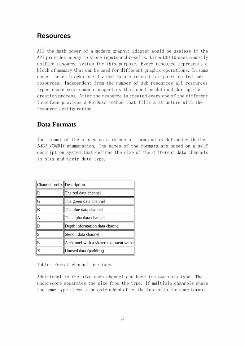
Data Formats

The format of the stored data is one of them and is defined with the

DXGI_FORMAT enumeration. The names of the formats are based on a self description system that defines the size of the different data channels

in bits and their data type.

Channel prefix Description

R The red data channel

G The green data channel

B The blue data channel

A The alpha data channel

D Depth information data channel

S Stencil data channel

E A channel with a shared exponent value

X Unused data (padding)

Table: Format channel prefixes

Additional to the size each channel can have its own data type. The

underscore separates the size from the type. If multiple channels share

the same type it would be only added after the last with the same format.

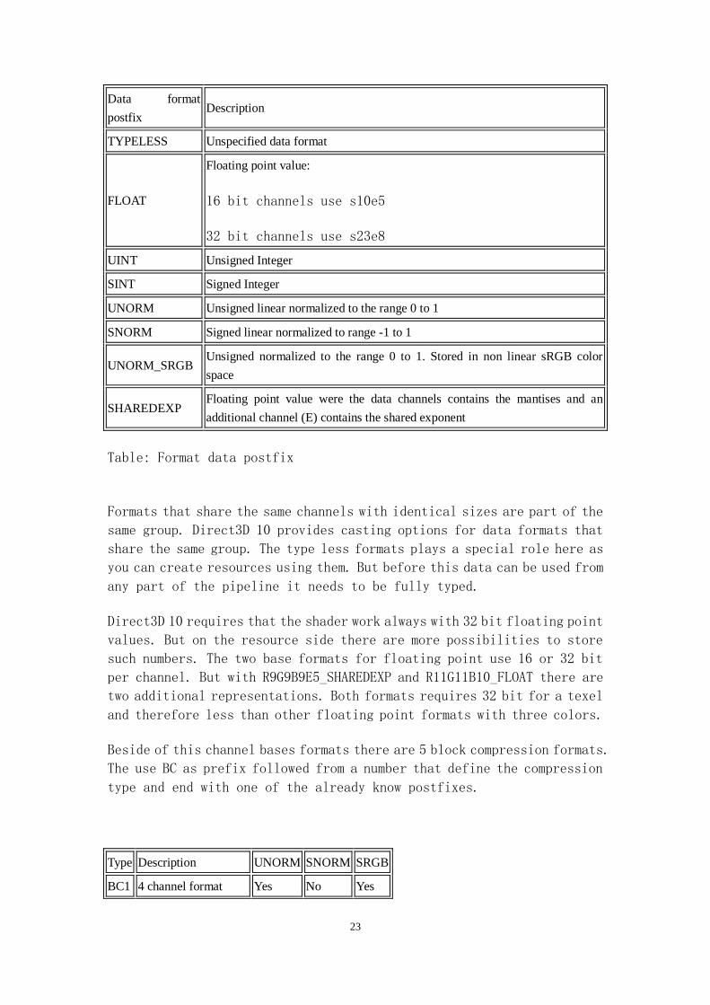
23

Data format

postfix Description

TYPELESS Unspecified data format

FLOAT

Floating point value:

16 bit channels use s10e5

32 bit channels use s23e8

UINT Unsigned Integer

SINT Signed Integer

UNORM Unsigned linear normalized to the range 0 to 1

SNORM Signed linear normalized to range -1 to 1

UNORM_SRGB Unsigned normalized to the range 0 to 1. Stored in non linear sRGB color

space

SHAREDEXP Floating point value were the data channels contains the mantises and an

additional channel (E) contains the shared exponent

Table: Format data postfix

Formats that share the same channels with identical sizes are part of the

same group. Direct3D 10 provides casting options for data formats that

share the same group. The type less formats plays a special role here as

you can create resources using them. But before this data can be used from

any part of the pipeline it needs to be fully typed.

Direct3D 10 requires that the shader work always with 32 bit floating point

values. But on the resource side there are more possibilities to store

such numbers. The two base formats for floating point use 16 or 32 bit

per channel. But with R9G9B9E5_SHAREDEXP and R11G11B10_FLOAT there are

two additional representations. Both formats requires 32 bit for a texel

and therefore less than other floating point formats with three colors.

Beside of this channel bases formats there are 5 block compression formats.

The use BC as prefix followed from a number that define the compression

type and end with one of the already know postfixes.

Type Description UNORM SNORM SRGB

BC1 4 channel format Yes No Yes

24



BC4 Two channel format Yes Yes No

BC5 Single channel format Yes Yes No

Table: Block compression types.

The block size for these formats is always 4x4 texels and every block need

64 or 128 bit in compressed form. There are three basis compression schemes.

The first one encodes a three channel color value. It provides a 4 bit

linear interpolation between two 16 bit colors. The first three block

compression formats make use of it. As an alternative one bit can be used

as alpha value in the first block compression format that doesn't provide

an explicit alpha channel.

The alpha channels can be stored either as 4 bit per texel or a 3 bit linear

interpolation between two 8 bit values. BC2 use the 4 bit version and BC3

the 3 bit interpolation.

The last two block compression formats doesn't contain a color compression

block at all. They use one or two of the linear alpha compression blocks

to represent general data.

Based on these generic name conventions Direct3D 10 provides a limited

set of valid formats. Additional formats are not part of specification

and therefore not supported.

Resource Usage

To create every resource in the right memory area Direct3D 10 expect an

indication how it will later used. There are four different predefined

cases. A Resource can flag as Immutable if it will never changed it content after creation. For that reason you need to provide the content already

as part of the creation process. For a slow rate of change Direct3D knows

the Default usage. Dynamic is the right choice if the resource will updated multiple times per frame. If it is used to transfer data back from the

GPU Direct3D 10 provides a special Staging usage type. Additional the

usage limits the access rights of the CPU and GPU for theses resources.

25

Usage Description CPU

Access

GPU

Access

D3D10_USAGE_IMMUTABLE Resource content is never updated

after creation. None Read

D3D10_USAGE_DEFAULT Resource content change not faster

than once per frame. None Read/Write

D3D10_USAGE_DYNAMIC Resource content change multiple

times per frame. Write Read

D3D10_USAGE_STAGING Resource is used to transfer data to

and from the GPU. Read/Write Only copy

Table: Resource Usage

26

Resource Binding

Figure 4: Pipeline Binding Points.

The Direct3D pipeline offers multiple points were resources can connected.

While some of them accept only one resource at the same time others

provides multiple slots. Depending on the used connection the graphics

processor will read, write or do both with the data behind the resource.

Although the unified memory system allows connecting most resources at

every point it is necessary to define all connection points were a resource

would use in advanced during resource creation.

27

Binding

point

Slot

cou

nt

Access Bind flag Set-Method Get-Method

Index

Buffer 1 Read

D3D10_BIND_INDEX_BUF

FER IASetIndexBuffer IAGetIndexBuffer

Vertex

Buffer 16 Read

D3D10_BIND_VERTEX_BU

FFER

IASetVertexBuffe

rs

IAGetVertexBuffe

rs

Vertex

ShaderCons

tant Buffer

16 Read D3D10_BIND_CONSTANT_

BUFFER

VSSetConstantBu

ffers

VSGetConstantB

uffers

Vertex

ShaderShad

er Resource

128 Read D3D10_BIND_SHADER_RE

SOURCE

VSSetShaderRes

ources

VSGetShaderRes

ources

Geometry

ShaderCons

tant Buffer


BUFFER

GSSetConstantBu

ffers

GSGetConstantB

uffers

Geometry

ShaderShad

er Resource


SOURCE

GSSetShaderRes

ources

GSGetShaderRes

ources

Stream Out

Target 4 Write

D3D10_BIND_STREAM_OU

TPUT SOSetTargets SOGetTargets

Pixel

ShaderCons

tant Buffer


BUFFER

PSSetConstantBu

ffers

PSGetConstantBu

ffers

Pixel

ShaderShad

er Resource


SOURCE

PSSetShaderReso

urces

PSGetShaderReso

urces

Depth

Stencil 1

Read/W

rite

D3D10_BIND_DEPTH_STE

NCIL

OMSetRenderTar

gets

OMGetRenderTar

gets

Render

Target 8

Read/W

rite

D3D10_BIND_RENDER_TA

RGET

OMSetRenderTar

gets

OMGetRenderTar

gets

All 3 shader stages use the same two binding point types. The constant

buffers are used as the primary memory for the uniform shader variables.

The shader resource binding points can be used to bind resources like

textures.

Beside of D3D10_BIND_CONSTANT_BUFFER multiple bind flags can be combined to allow resources to be used on different bind points. This leads to the

potential situation were one resource is connected to multiple different

binding points. This is allowed as long as the configuration doesn't cause

28

a read/write hazard on the same memory block. Therefore you can't use a

resource as Render Target and Shader Resource or any other read write

combination at the same time. It is although not valid to bind the same

sub resources to multiple write points for one draw call. If you try to

break these rules Direct3D 10 will enforce it by solving the hazard

condition. After this you will noticed that some resources are not longer

bound.

Another limiting factor for the bind point selection is the usage type.

As staging resources could not use form the graphics processor you

couldn't define any binding. Immutable and dynamic resources could only

used for GPU read only operations.

Default Dynamic Immutable Staging

Index Buffer OK OK OK

Vertex Buffer OK OK OK

Constant Buffer OK OK OK

Shader Resource OK OK OK

Stream Out OK

Depth Stencil OK

Render Target OK

Buffer

The simplest Direct3D 10 resource type is the Buffer. It represents a plain type less block of memory without additional sub resources. Additional

to the common properties you need only define the overall buffer size in

bytes during creation.

As any other resource the device is responsible to create it. The

CreateBuffer method will take the full description that is stored in a

D3D10_BUFFER_DESC structure. If you want to create an immutable buffer

you have to provide initial data for it. In other cases this is an option.

As last parameter you have to provide a pointer to a parameter were

Direct3D can store the ID3D10Buffer interface pointer. If you pass a NULL

pointer along the runtime would not create the resource but it will

validate the creation parameters.

The ID3D10Buffer interface contains only a small count of member functions.

GetDesc will fill a D3D10_BUFFER_DESC with the values that were used to

29

create the resource. We will discuss the two other methods Map and UnMap

later.

Texture 1D

As the 1D texture is a texture type you have to specify a format for its

elements. Like a buffer it requires a width but this time it doesn't

specify the size in bytes. Instead it defines the number of elements from

the selected format. Direct3D 10 can optional create a mip map chain for

you. These elements of this chain are accessible as consecutive sub

resources. Another option to create sub resources is the texture array.

Instead of adding additional smaller blocks of memory every element in

the array will have the same width.

Figure 5: Texture 1D with mip maps and as array.

Creating a 1d texture is very similar to creating a buffer. You need to

take additional care if you want to provide initial data. Like the

CreateBuffer method CreateTexture1D takes a pointer to a

D3D10_SUBRESOURCE_DATA structure. But this time it needs to point to the

first element of an array with one element for every sub resource your

texture will contain.

30

Texture 2D

The 2D texture type adds an additional dimension to its smaller brother.

It's although the only resource type that supports multi sampling. But

you can't use multi sampling together with arrays or mip maps.

Figure 6: Texture 2D.

Direct3D 10 doesn't have a dedicated cube texture type. To get one you

need to create a Texture 2D array with 6 elements and use the additional

D3D10_RESOURCE_MISC_TEXTURECUBE flag. This tells the API that these

elements should use as the six faces of a cube. As the array parameter

is already blocked you can't create an array of cubes. But mip maps are

still supported.

31

Figure 7: Texture 2D as Cube.

Again CreateTexture2D works like the other resource creation methods and

the ID3D10Texture2D interface offers the same methods.

Texture 3D

The last offered resource type supports three dimensions. The only way

to create additional sub resources is mipmaping. There is no support for

arrays or multisampling

Figure 8: Texture 3D with Mip maps.

32

Resource limitations

Beside the valid combinations of creation parameters Direct3D 10 defines

some additional limitations for resources. Each size of a 1D and 2D texture

are limited to 8192 elements. For 3D resources only 2048 elements per

dimension are allowed. In any case no resources could be requiring more

than 128 MB memory.

Sub resources

Every time you want refer to a sub resource you need to now its number.

This is easy when a resource have only mip maps or only have array elements

of the same size. But if you have both at the same time you need to calculate

the number. To do this you have to multiple the numbers of mip maps per

element with the element you want and add the mip map level. To make this

step easier for you the Direct3D 10 header contains the function

D3D10CalcSubresource.

Update Resources

After you have created a resource Direct3D 10 provides different ways to

update their content as long as they are not defined as Immutable. With the UpdateSubresource method Direct3D 10 can copy a block of memory to a part or a whole sub resource. In the case your resource was created

without CPU write access this is the only way for the CPU to change the

content after it have created. As UpdateSubresource can transfer data to

any kind of resource it use a box to specify the target position and take

to pitch values. These parameters will use depended on the number of real

dimension of the resource. UpdateSubresource guaranteed that the Direct3D

10 will not use the system memory after it returns. At the same time it

makes sure that it does not stall if the data cannot be copied immediately.

In such cases it will make an extra copy to an internal buffer. The final

copy to the real resource will be scheduled as part of the regular

asynchrony command stream.

Copy between Resources

Instead of a memory block you can use another resource as source for a

copy operation. With the CopyResource method a resource with all sub resources will be transferred. CopySubresourceRegion allows copying only a section of a sub resource to another one. Both methods requires that

33

you use resources from the same type as source and destination. If you

copy from one texture to another the formats must be part of the same format

group. As CopyResource cannot stretch both resources must be same size. CopySubresourceRegion can be used with different size but as its brother it will make only a one to one copy. All copy operations will be executed

asynchrony. Therefore you will not get any result. If you try to make an

illegal copy it will fail silent. But the debug layer will check all

parameters that are part of a copy operation and report such errors.

Some common mistakes when using the CopyResource method are:

// try to copy a resource to itself

device->CopyResource (pBuffer, pBuffer);

// use an immutable resource as target

device->CopyResource (pImmutableBuffer3, pDefaultBuffer);

// Destination and source have different sizes

device->CopyResource (p100ByteBuffer, p200ByteBuffer);

// use different resource typesdevice->CopyResource

(pTexture, pBuffer);

// use incompatible formats

device->CopyResource (pFloatTexture, pUNormTexture);

// use a multisample texture as source or target

device->CopyResource (pMultisampleTexture,

pOneSampleTexture);

// use resources with different mip map counts

device->CopyResource (pOneMipMapTexture,

pFullMipMapsTextzre);

As CopySubresourceRegion allows you to specify a destination position and

a source box gives you can work around some of the CopyResource limitations

but most of them are still valid. As UpdateResource the method could be

used with every kind of resource and therefore not every parameter is

always used.

With ResolveSubresource

Direct3D 10 supports another method that can transfer data from one sub

resource to another. But this one will do more than a simple copy. During

the copy the multiple samples in the source will be reduced to a single

34

sample for the destination. This is necessary to make the content of a

multisampled resource accessible as a normal texture for future

processing. Beside of the different sample count the two sub resources

that are used for the resolve operation need to be compatible. This

requires the same size and cast able data formats. As ResolveSubresource

works with typeless resources the function let you select the format that

should be used to calculate the single sample in the right way. But like

the sub resources self this format have to be cast able.

Map Resources

The content of resources that are created as dynamic or staging can be

mapped in the CPU memory space for direct access. But reading operations

for theses memory blocks are limited to staging resources. Dynamic

resources support only different write modes instead. You can either

request a new memory block and discard anything that was written to the

resource before or map with the promise to not overwrite anything you have

already changed since the last discard. As Direct3D 10 has only limited

access to mapped resources they need to be unmapped before they can used

again.

Since each type of resource has a different memory layout the Map and Unmap

methods are part of the resource specific interfaces. Independent from

the type each Map method takes the required access level. If the resource

is a texture and therefore could contain sub resources you have additional

select one of them. Finally each Map method fills a provided variable with

details how the data is mapped. If the resource has only one dimension

(Buffers, 1D Texture) Direct3D 10 will only return a pointer to the first

element. For a 2D Texture it additional delivers the size of each line

in bytes. The size for a whole plane is added for 3D textures.

Resource type Sub

resource Result type

Buffer (ID3D10Buffer) No void* (data)

1D Texture

(ID3D10Texture1D) Yes void* (data)

2D Texture

(ID3D10Texture2D) Yes D3D10_MAPPED_TEXTURE2D(row pitch, data)

3D Texture

(ID3D10Texture2D) Yes

D3D10_MAPPED_TEXTURE3D(row pitch, depth

pitch, data)

35

Table mapping methods

To finish the work with a mapped resource a call to the Unmap method is

required. Beside the sub resource identifier for textures it doesn't need

any other parameter. If the resource has more than one dimension the

mapping methods will return pitch information's. You need these values

to calculate the start address of the lines and slices as Direct3D 10

doesn't give you a guaranty that there are no padding bytes used.

D3D10_MAPPED_TEXTURE2D Mapped;

if (pTexture2D->Map (0, D3D10_MAP_WRITE_DISCARD, 0, &Mapped)

== S_OK)

{

for<nowiki> (UINT Y = 0 ; Y < height ; Y++)</nowiki>

{

BYTE* pLine =

&((BYTE*)Mapped.pData)[Y*Mapped.RowPitch];

for (UINT X = 0 ; X < width ; X++)

{

// Set the texel using pLine and X

}

}

pTexture2D->Unmap (0);

}

D3D10_MAPPED_TEXTURE3D Mapped;

if (pTexture3D->Map (0, D3D10_MAP_WRITE_DISCARD, 0, &Mapped)

== S_OK)

{

for (UINT Z = 0 ; Z < depth ; Z++)

{

for (UINT Y = 0 ; Y < height ; Y++)

{

BYTE* pLine =

&((BYTE*)Mapped.pData)[Z*Mapped.DepthPitch +

Y*Mapped.RowPitch];

for (UINT X = 0 ; X < width ; X++)

{

// Set the texel using pLine and X

}

}

36

}

pTexture3D->Unmap (0);

}

Views

As a resource and it's subresources are only blocks of memory it is often

necessary to give Direct3D 10 more details about how it should be used.

This is done with one of three view types. Two of them are only used by

the Output Merger to access the depth stencil buffer and the render targets.

OMSetRenderTargets will set up to eight render target views and one depth

stencil view with one call. Every time you call OMSetRenderTargets it will

override everything. If you need to know the currently active views

OMGetRenderTargets will give you the answer.

The remaining view type is used for any of the 3 shader stages in the

pipeline. Each one have 128 slots that can be Set with

XXSetShaderResourceView were the XX stands for the stage that should be

accessed. In comparison to the output merger calling this method will not

reset the current configuration. Only the selected range of views is

updated.

But these slots are only used for resources that are accessed by one of

the HLSL read functions. The constant buffers that have a fixed format

don't need a view. XXSetConstantBuffer takes buffers that are not

encapsulated with a view. Like XXSetShaderResourceViews the 16 slots can

be updated individual. The same is true for the vertex and index buffer

that are used from the input assembler. IASetVertexBuffers and

IASetIndexBuffer use raw buffers without a view. As you can have up to

16 vertex streams but only one index buffer only IASetVertexBuffers allows

you to define a start slot and range.

If you need a view it should created in advanced like the resource it

reference. As the following table shows there are some limitations which

resource types a view can contain. Beside of the base resource type a view

although different between resources that store arrays or use

multisampling. 2D Textures that are flagged as cube map need special

handling too.

Resource type Shader resource

view

Render target

view

Depth stencil

view

37

Buffer Yes Yes No

Texture 1D Yes Yes Yes

Texture 1D as Array Yes Yes Yes

Texture 2D Yes Yes Yes

Texture 2D as Array Yes Yes Yes

Texture 2D with Multisampling Yes Yes Yes

Texture 2D with Multisampling as

Array Yes Yes Yes

Texture 3D Yes Yes No

Texture 2D as Cube Yes No No

Additional to the view dimension you have to provide a format that should

be used to access the resource. It needs to be from the same format group

that is used by the raw resource and fully typed. Therefore you can't use

any format that contains a TYPELESS in its name. If your raw resources

already use a valid view format you can use DXGI_FORMAT_UNKNOWN and it

will be used for the view too. In this case you can even provide a NULL

as description and Direct3D 10 will create a view to the full resource.

In any other case the create methods need depending on the selected view

dimension more information's.

As a buffer contains only one sub resource it will be selected

automatically but you can define the offset of the first element and the

number of elements that the user of the view will see. Both values are

specified in elements that are depending on the view format and not in

bytes like the size of the buffer resource.

Figure 9: Buffer View.

1D texture can contain multiple mip maps as sub resource. As render targets

and depth stencil buffers can only access one level in the chain the mip

map need to specify. When the texture used as shader input a range of

accessible mip maps could be selected.

38

Figure 10: 1D Texture View.

If the 1D texture contains an array of textures the view can limit the

accessible elements.

39

Figure 11: 2D Texture View.

As long as a 2D texture is not created with multisample elements it behaves

like a 1D textures during the view creation. As 2D textures with

multisampling doesn't support mip maps there is no need to specified which

mip maps would be part of the view.

A view doesn't care about the additional dimension of the 3D texture and

you can select a range of mip maps that should be part of the view.

Shader resource views for cube textures are special cases. Even as an array

with 6 elements you can only select the mip map range as all faces are

part of the view as default.

40

But you can although create a view without any description. If you use

a NULL pointer instead Direct3D will use a default configuration based

on the provided raw resource.

An additional service that the create methods provide is a parameter check.

If you don't provide a pointer to store the interface pointer to a newly

created view Direct3D 10 will only check if your resource and description

match all requirements without create the view.

State Objects

Direct3D 10 use state objects to control the non programmable parts of

the pipeline. As the control different parts the five state object types

differs in their details but there are some general aspects that are valid

for every type. Like the Direct3D resources every state object is a full

COM object with its own reference counter. It needs to be explicit created

and destroyed. As creation could be an expensive operation it should be

done in advance like memory based resource and shader creation. But there

is a limit how much state objects could be created per device. Direct3D

10 allows you to have 4096 state objects from any type. To make it easier

to stay inside this limitation Direct3D does only create a new state object

that contented against this limit if you haven't already created an object

with the same configuration. In the case there is already a matching state

object the create function will return it. You still have to release it

at the end because the internal reference count would be increased.

Input Layout

The Input Layout state object is a special case in this group of five.

While the other four are only containers for multiple states the input

layout is more complex. It is responsible to manage the transfer from the

assigned vertex buffers to the input registers of the vertex shader. To

do this job it needs detailed information's about the layout of the vertex

buffers and the input registers that the shader use. To make your life

easier the create method will extract the necessary register information

direct from a provided shader in its byte code form. But the vertex buffer

layout needs still to be described with an array of

D3D10_INPUT_ELEMENT_DESC structures. Each array element stands for one

entry in the buffers. Beside of the semantic information that is necessary

to bind everything together the D3D10_INPUT_ELEMENT_DESC structures

contains the information about the input assembler slot were the buffer

will be assigned, the format of the data and the offset from the beginning

41

of the vertex. Additional it provides the option to use the same values

for multiple instances.

Figure 12: Input Layout State.

The semantic information's that are used to link the vertex data to the

shader inputs are stored as human readable strings. During the creation

process Direct3D 10 will look up the provided element array to find for

each of the shader input registers the matching counterpart. Then it will

pass this information to the driver which will build a fixed transfer

description for later usage. This will free Direct3D 10 to build the right

linking every time something is drawn but it force the application to

create an own input layout for every used combination of vertex buffer

layouts and shader input registers.

Rasterizer

The rasterizer state object is a collection of 10 states that control the

behavior of the rasterizer pipeline state. As the rasterizer is

responsible to finally build the primitives from the provided vertices

and convert them to pixel the states cover this whole process.

42

Figure 13: Rasterizer State.

Depth Stencil State

Every pixel that survives the pixel shading process will end up in the

output merger were one part of the following operations are done from a

depth stencil unit that is controlled by a depth stencil state object.

This object contains three states that control the depth operations and

additional eleven states for the two-side stencil operations.

43

Figure 14: Depth Stencil State.

As the stencil unit requires a reference value that is not part of the

state object you need to provide it every time the depth stencil state

object is assigned to the pipeline with OMSetDepthStencilState.

Blend State

The second part of the output merger stage is configured with a blend state

object. These collections of nine states control how the up to 8 pixel

shader outputs should be stored in the assigned target resources.

44

Figure 15: Blend State.

Again this unit needs more states than the state object contains. They

blend factor and multi sample mask need to provide during the activation

of the state object with OMSetBlendState.

Sampler State

The sampler state object is another special kind of state object. As every

other one it is responsible to control a fixed function unit in the

pipeline but it is used together with the programmable shader stages.

Another peculiarity is that every one of the three shader stages provides

16 slots for sampler stages objects. Therefore it is the only state object

type that can have more than one active object at the same time. The ten

states it groups together control how a sampler unit that is part of a

45

shader unit should read the data that is accessible over a shader resource

view.

Figure 16: Sampler State.

Shaders

Any stage that is not configured with a state object needs a shader program

to process the data. Typical programs contain sections that calculate

positions, texture coordinates or colors.

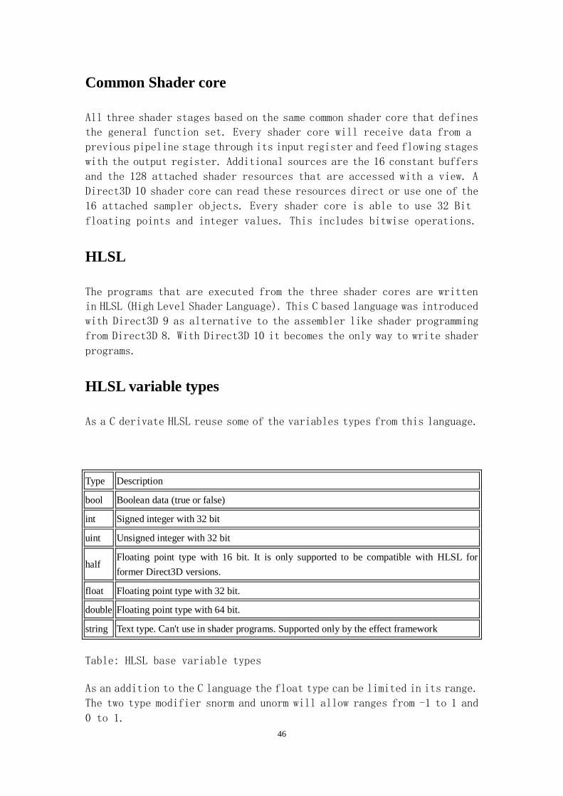
46

Common Shader core

All three shader stages based on the same common shader core that defines

the general function set. Every shader core will receive data from a

previous pipeline stage through its input register and feed flowing stages

with the output register. Additional sources are the 16 constant buffers

and the 128 attached shader resources that are accessed with a view. A

Direct3D 10 shader core can read these resources direct or use one of the

16 attached sampler objects. Every shader core is able to use 32 Bit

floating points and integer values. This includes bitwise operations.

HLSL

The programs that are executed from the three shader cores are written

in HLSL (High Level Shader Language). This C based language was introduced

with Direct3D 9 as alternative to the assembler like shader programming

from Direct3D 8. With Direct3D 10 it becomes the only way to write shader

programs.

HLSL variable types

As a C derivate HLSL reuse some of the variables types from this language.

Type Description

bool Boolean data (true or false)

int Signed integer with 32 bit

uint Unsigned integer with 32 bit

half Floating point type with 16 bit. It is only supported to be compatible with HLSL for

former Direct3D versions.

float Floating point type with 32 bit.

double Floating point type with 64 bit.

string Text type. Can't use in shader programs. Supported only by the effect framework

Table: HLSL base variable types

As an addition to the C language the float type can be limited in its range.

The two type modifier snorm and unorm will allow ranges from -1 to 1 and

0 to 1.

47

Another difference from C is the native support of vector and matrix

variable types. You can use every base type to create vectors with up to

four elements and matrices with any size up to 4 elements in both

directions. There are two different way to specify a vector or matrix

You can add the number of rows and columns to the name of the base type

float2 texture;

float4 position;

float1 color;

float4x4 view;

A vector or a matrix with a size of one is not the same as the base type.

The more complex syntax use the template syntax known from C++

vector <float,2> texture;

vector <float,4> position;

vector <float,1> color;

matrix <float, 4, 4> view;

To define more complex types you can combine base, vector and matrix types

together to structs.

struct Input

{

float3 Position;

float3 Normal;

float2 Texturecoordinates;

};

The last C element that made it in HLSL is the typedef.

HLSL functions

To declare and define a function HLSL is following C but made some changes.

Each parameter that is part of the function parameter list can have an

additional modifier.

modifier Description

in The parameter is only used as input.

48

out The parameter is only used as output.

inout The parameter is used in both directions.

uniform Uniform parameters are provided form the CPU and stay the same for all elements that

are part of the same draw call.

Table: HLSL function parameter modifier

Whenever it was possible HLSL implements a function from the common C

runtime library in the same way that is already know. Other functions are

new as there is no counterpart in C. But the number of both types is limited

Name Syntax Description

abs abs(value a) Absolute value (per component).

acos acos(x)

Returns the arccosine of each

component of x. Each component

should be in the range [-1, 1].

all all(x) Test if all components of x are

nonzero.

any any(x) Test if any component of x is

nonzero.

append append(x) Append data to the geometry shader

out stream.

asfloat asfloat(x) Convert the input type to a float.

asin asin(x)

Returns the arcsine of each

component of x. Each component

should be in the range [-pi/2, pi/2].

asint asint(x) Convert the input type to an integer.

asuint asuint(x) Convert the input type to an

unsigned integer.

atan atan(x)

Returns the arctangent of x. The

return values are in the range [-pi/2,

pi/2].

atan2 atan2(y, x)

Returns the arctangent of y/x. The

signs of y and x are used to

determine the quadrant of the return

values in the range [-pi, pi]. atan2 is

well-defined for every point other

than the origin, even if x equals 0

49

and y does not equal 0.

ceil ceil(x) Returns the smallest integer which

is greater than or equal to x.

clamp clamp(x, min, max) Clamps x to the range [min, max].

clip clip(x)

Discards the current pixel, if any

component of x is less than zero.

This can be used to simulate clip

planes, if each component of x

represents the distance from a

plane.

cos cos(x) Returns the cosine of x.

cosh cosh(x) Returns the hyperbolic cosine of x.

cross cross(a, b) Returns the cross product of two 3D

vectors a and b.

D3DCOLORtoUBYTE4 D3DCOLORtoUBYTE4(x)

Swizzles and scales components of

the 4D vector x to compensate for

the lack of UBYTE4 support in

some hardware.

ddx ddx(x)

Returns the partial derivative of x

with respect to the screen-space

x-coordinate.

ddy ddy(x)

Returns the partial derivative of x

with respect to the screen-space

y-coordinate.

degrees degrees(x) Converts x from radians to degrees.

determinant determinant(m) Returns the determinant of the

square matrix m.

distance distance(a, b) Returns the distance between two

points, a and b.

dot dot(a, b) Returns the dot product of two

vectors, a and b.

exp exp(x) Returns the base-e exponent.

exp2 value exp2(value a) Base 2 Exp (per component).

faceforward faceforward(n, i, ng) Returns -n * sign(â€¢(i, ng)).

floor floor(x) Returns the greatest integer which

is less than or equal to x.

fmod fmod(a, b)

Returns the floating point

remainder f of a / b such that a = i *

b + f, where i is an integer, f has the

50

same sign as x, and the absolute

value of f is less than the absolute

value of b.

frac frac(x)

Returns the fractional part f of x,

such that f is a value greater than or

equal to 0, and less than 1.

frexp frexp(x, exp)

Returns the mantissa and exponent

of x. frexp returns the mantissa, and

the exponent is stored in the output

parameter exp. If x is 0, the

function returns 0 for both the

mantissa and the exponent.

fwidth fwidth(x) Returns abs(ddx(x)) + abs(ddy(x))

isfinite isfinite(x) Returns true if x is finite, false

otherwise.

isinf isinf(x) Returns true if x is +INF or -INF,

false otherwise.

isnan isnan(x) Returns true if x is NAN or QNAN,

false otherwise.

ldexp ldexp(x, exp) Returns x * 2exp

length length(v) Returns the length of the vector v.

lerp lerp(a, b, s)

Returns a + s(b - a). This linearly

interpolates between a and b, such

that the return value is a when s is

0, and b when s is 1.

lit lit(n dot l, n dot h, m)

Returns a lighting vector (ambient,

diffuse, specular, 1):ambient =

1;diffuse = (n â€¢ l < 0) ? 0 : n dot

l; specular = (n dot l < 0)

(n dot

h <

0) ?

0 : (n

dot h

* m);

log log(x)

Returns the base-e logarithm of x. If

x is negative, the function returns

indefinite. If x is 0, the function

returns +INF.

log10 log10(x)

Returns the base-10 logarithm of x.

If x is negative, the function returns


returns +INF.

log2 log2(x) Returns the base-2 logarithm of x. If

51

x is negative, the function returns


returns +INF.

max max(a, b) Selects the greater of a and b.

min min(a, b) Selects the lesser of a and b.

modf modf(x, out ip)

Splits the value x into fractional and

integer parts, each of which has the

same sign and x. The signed

fractional portion of x is returned.

The integer portion is stored in the

output parameter ip.

mul mul(a, b)

Performs matrix multiplication

between a and b. If a is a vector, it

is treated as a row vector. If b is a

vector, it is treated as a column

vector. The inner dimension

acolumns and brows must be equal.

The result has the dimension arows

x bcolumns.

noise noise(x) Not yet implemented.

normalize normalize(v)

Returns the normalized vector v /

length(v). If the length of v is 0, the

result is indefinite.

pow pow(x, y) Returns xy.

radians radians(x) Converts x from degrees to radians.

reflect reflect(i, n)

Returns the reflection vector v,

given the entering ray direction i,

and the surface normal n, such that

v = i - 2n * (iâ€¢n).

refract refract(i, n, R)

Returns the refraction vector v,

given the entering ray direction i,

the surface normal n, and the

relative index of refraction R. If the

angle between i and n is too great

for a given R, refract returns (0,0,0).

restartstrip restartstrip() Restart the current primitive strip

and start a new primitive strip.

round round(x) Rounds x to the nearest integer

rsqrt rsqrt(x) Returns 1 / sqrt(x)

saturate saturate(x) Clamps x to the range [0, 1]

52

sign sign(x)

Computes the sign of x. Returns -1

if x is less than 0, 0 if x equals 0,

and 1 if x is greater than zero.

sin sin(x) Returns the sine of x

sincos sincos(x, out s, out c)

Returns the sine and cosine of x.

sin(x) is stored in the output

parameter s. cos(x) is stored in the

output parameter c.

sinh sinh(x) Returns the hyperbolic sine of x

smoothstep smoothstep(min, max, x)

Returns 0 if x < min. Returns 1 if

x > max. Returns a smooth Hermite

interpolation between 0 and 1, if x

is in the range [min, max].

sqrt value sqrt(value a) Square root (per component)

step step(a, x) Returns (x >= a) ? 1 : 0

tan tan(x) Returns the tangent of x

tanh tanh(x) Returns the hyperbolic tangent of x

tex1D tex1D(s, t) 1D texture lookup. s is a sampler or

a sampler1D object. t is a scalar.

tex1Dgrad tex1Dgrad(s, t, ddx, ddy)

1D gradient texture lookup. s is a

sampler or sampler1D object. t is a

4D vector. The gradient values

(ddx, ddy) select the appropriate

mipmap level of the texture for

sampling.

tex1Dlod tex1Dlod(s, t)

1D texture lookup with LOD. s is a


4D vector. The mipmap LOD is

specified in t.

tex1Dproj tex1Dproj(s, t)

1D projective texture lookup. s is a


4D vector. t is divided by its last

component before the lookup takes

place.

tex2D tex2D(s, t)

2D texture lookup. s is a sampler or

a sampler2D object. t is a 2D

texture coordinate.





53



sampling.





specified in t.


2D projective texture lookup. s is a


4D vector. t is divided by its last

component before the lookup takes

place.

tex3D tex3D(s, t)

3D volume texture lookup. s is a

sampler or a sampler3D object. t is

a 3D texture coordinate.







sampling.





specified in t.


3D projective volume texture

lookup. s is a sampler or sampler3D

object. t is a 4D vector. t is divided

by its last component before the

lookup takes place.

texCUBE texCUBE(s, t)

3D cube texture lookup. s is a

sampler or a samplerCUBE object. t

is a 3D texture coordinate.

texCUBEgrad texCUBEgrad(s, t, ddx,

ddy)

3D gradient cube texture lookup. s

is a sampler or samplerCUBE

object. t is a 4D vector. The gradient

values (ddx, ddy) select the

appropriate mipmap level of the

texture for sampling.

texCUBElod tex3Dlod(s, t) 3D 3D cube texture lookup with

LOD. s is a sampler or

54

samplerCUBE object. t is a 4D

vector. The mipmap LOD is

specified in t.

texCUBEproj texCUBEproj(s, t)

3D projective cube texture lookup. s

is a sampler or samplerCUBE

object. t is a 4D vector. t is divided

by its last component before the

lookup takes place.

transpose transpose(m)

Returns the transpose of the matrix

m. If the source is dimension

mrows x mcolumns, the result is

dimension mcolumns x mrows.

Table: HLSL intrinsic functions

HLSL classes

Even primary C based HLSL know C++ like object classes. One for each shader

resource type and another for the output stream that is written by a

geometry shader.

For every valid type that can be used in a shader resource view object

there is an HLSL object class

HLSL type Shader resource view type Description

Buffer D3D10_SRV_DIMENSION_BUFFER A buffer resource.

Texture1D D3D10_SRV_DIMENSION_TEXTURE1D A one dimension

texture.

Texture1DArray D3D10_SRV_DIMENSION_TEXTURE1DARRAY An array of one

dimension textures.

Texture2D D3D10_SRV_DIMENSION_TEXTURE2D A two dimension

texture.

Texture2DArray D3D10_SRV_DIMENSION_TEXTURE2DARRAY An Array of two

dimension textures.

Texture2DMS D3D10_SRV_DIMENSION_TEXTURE2DMS

A two dimension

texture with multi

sampling

Texture2DMSArray D3D10_SRV_DIMENSION_TEXTURE2DMSARRAY An Array of two

55

dimension textures

with multi sampling

Texture3D D3D10_SRV_DIMENSION_TEXTURE3D A three dimension

texture

TextureCube D3D10_SRV_DIMENSION_TEXTURECUBE A cube texture

The HLSL shader resource objects support the following methods.

Method Description

GetDimensions Report the width, height and number of mip maps. Cannot be used with

views that represent a buffer.

Load Load a texture value without using a sampler.

Sample Use a sampler to read from a texture.

SampleCmp Like Sample but this method does an additional compare against a provide

reference value.

SampleCmpLevelZero Works like SampleCmp but will only use the zero mip map level.

SampleGrad Use provided gradients for the sample instead of calculate them.

SampleLevel Sample from a specified level.

Table: HLSL texture object methods

HLSL flow control attributes

As extension some of the C flow control statements support attributes to

control how the compiler should handle them.

for/while

o unroll (x)instead of insert loop instructions the compiler will unroll the loop.

o loopthe compiler use a real loop

if

o branchinsert code that let the shader decide at runtime which side should taken.

o flattenAlways calculate both sides and decide then which results are used.

switch

o branchconverts the switch to a cascade of if instructions that are use the

â€œbranchâ€� attribute.

o flattenexecute all cases and decide at the end which results are zaken.

o forcecaseforce the compiler to use a real hardware case.

56

o callthe compiler will generate a sub function for each case.

Geometry Shader

If a shader will be used on the geometry shader stage it could use two

additional HLSL functions.

Append: Adds an additional vertex to the output stream.

RestartStripe: Terminate the current striped primitive and start a new one.

To make use of them the shader function need a stream object as in out

parameter. HLSL knows three different types of stream objects:

PointStream

LineStream

TriangleStream

As template object types the need to use together with an structure that

describe the output vertex format. This could be different from the input

format.

As HLSL supports these two commands inside a loop a generic number of

vertexes could be outputted with each shader invocation. To allow the GPUs

future optimizations it is necessary to define the maximum number of

vertexes that will be generated.

[maxvertexcount(10)]

void GSMain(point GSIn input[1], inout PointStream<GSOut>

PointOutputStream)

{

...

}

Pixel Shader

A Direct3D 10 pixel shader is mostly identical to the common shader core.

But as the input values could base on the output of multiple vertex shaders

runs it needs additional information. Therefore HLSL provides 4

interpolation usage specifiers to manage this behavior.

57

Modifier Description

linear The values will be linear interpolated between the output values of the uses

vertices. This is the default modifier.

centroid Use centroid interpolation to improve results in the case of anti-aliasing.

nointerpolation Values will not be interpolated. Can only be used for integer variables.

Noperspective The values will be interpolated but without perspective correction.

Table: pixel shader interpolation modifiers

Compile Shader

Even with HLSL as the only way to program the shader stages it is still

necessary to compile your shader in a binary format before it could be

used to create the shader object. This makes it possible to do this

expensive operation ahead. As the compiler is part of the core runtime

you can compile all your shaders during the setup process. It is even

possible to compile the shader as part of the build process and only

include the binary code. In this case the HLSL code does not need to leave

the development system.

As already shown the common shader core is only the basic and each shader

stage have different limitations. Therefore it is necessary to tell the

compiler on which shader stage the result of the compilation will be later

used. Beside of adjust all check functions the selected profile will be

include in the binary shader for later use.

Additional to the primary output the compile method could deliver a human

readable list of errors and warnings.

Create Shader

In the end the binary shader code is used to create the real shader object.

It makes no difference if it was directly compiled or loaded from the disk.

In every case the runtime will check if the shader was compiled with the

right signature for the type you want to create. Additional there is a

hash signature that provides some kind protection against modification.

If it doesn't match the shader object will not be created.

To create a normal shader you will need only the binary code and the size

of it. But as there is no state object for the stream out unit like the

input layout object for the input assembler the information's need to

58

provide during the creation of the geometry shader that will generate the

output stream.

Reflect Shader

Instead of creating a shader object Direct3D 10 could create a shader

reflection object with the binary code. Beside of enumerate all input and

output registers you can query it for the resources that the shader consume.

This is useful if you want to write your own effect framework instead of

using the default one. Finally it gives you access to the statistical

information for the compiled shader.

The following example shows how to create a shader reflection and loop

over all elements it contains.

D3D10ReflectShader (pCode, CodeSize, &pReflector);

// General description first

pReflector->GetDesc (&ShaderDesc);

// enumerate the input elements

for (UINT Input = 0 ; Input < ShaderDesc.InputParameters ;

++Input)

{

pReflector->GetInputParameterDesc (Input, &InputDesc);

}

// enumerate the output elements

for (UINT Output = 0 ; Output < ShaderDesc.OutputParameters ;

++Output)

{

pReflector->GetOutputParameterDesc (Output,

&OutputDesc);

}

// enumerate the resource bindings

for (UINT Resource = 0 ; Resource < ShaderDesc.BoundResources ;

++Resource)

{

pReflector->GetResourceBindingDesc (Resource,

&ResourceDesc);

}

// enumerate the constant buffers

59

for (UINT Buffer = 0 ; Buffer < ShaderDesc.ConstantBuffers ;

++Buffer)

{

ID3D10ShaderReflectionConstantBuffer* pBuffer =

pReflector->GetConstantBufferByIndex (Buffer);

D3D10_SHADER_BUFFER_DESC BufferDesc;

pBuffer->GetDesc (&BufferDesc);

// enumerate the variables in the buffer

for (UINT Variable = 0 ; Variable < BufferDesc.Variables;

++Variable)

{

ID3D10ShaderReflectionVariable* pVariable =

pBuffer->GetVariableByIndex (Variable);

D3D10_SHADER_VARIABLE_DESC VariableDesc;

pVariable->GetDesc (&VariableDesc);

}

}

// Finally release the reflection object.

pReflector->Release ();

Direct3D 10 Device

As the former API versions Direct3D 10 is still based on a state machine.

The complete current context is stored in the device object. Each device

is bound to exactly one graphics adapter but you could have multiple device

objects per adapter. Every object that is created on a device can only

use together with this one even when you have two or more devices on the

same adapter. The only exceptions from this rule are shared resources.

But even if you create a resource as shared the object is exclusive bound

to its creator. You need to open the resource on the second device using

a shared handle to get a second object.

To tell Direct3D 10 that you need a shared resource you have to add

D3D10_RESOURCE_MISC_SHARED to the MiscFlags in the description. The

actual share handle can only be accessed with the IDXGIResource interface.

As there is only one open resource method for all type of resources it

is necessary to provide the type of interface that should be used for this

resource on the second device.

// Create a shareable texture

60

ID3D10Texture2D* pTexture2D = NULL;

D3D10_TEXTURE2D_DESC Texture2DDesc;

Texture2DDesc.Width = 1024;

Texture2DDesc.Height = 1024;

Texture2DDesc.MipLevels = 0;

Texture2DDesc.ArraySize = 1;

Texture2DDesc.Format = DXGI_FORMAT_R8G8B8A8_UNORM;

Texture2DDesc.SampleDesc.Count = 1;

Texture2DDesc.SampleDesc.Quality = 0;

Texture2DDesc.Usage = D3D10_USAGE_DEFAULT;

Texture2DDesc.BindFlags = D3D10_BIND_SHADER_RESOURCE;

Texture2DDesc.CPUAccessFlags = 0;

Texture2DDesc.MiscFlags = D3D10_RESOURCE_MISC_SHARED;

pD3D10Device->CreateTexture2D (&Texture2DDesc, NULL,

&pTexture2D);

// Get the handle

IDXGIResource* pResource;

pTexture2D->QueryInterface (__uuidof(IDXGIResource),

(void**)&pResource);

HANDLE resourceHandle;

pResource->GetSharedHandle (&resourceHandle);

// Transfer the Handle

// Open the resource

ID3D10Texture2D* pSharedTexture2D;

pD3D10Device2->OpenSharedResource (resourceHandle,

__uuidof(ID3D10Texture2D), (void**)&pSharedTexture2D);

In any cases theses resource interfaces are provided to the device

interface to configure the 3D pipeline. As there are multiple different

stages most method names starts with a two character code that identify

the stage. The three shader stages are all based on the common shader core

and share most methods names after the two character code. As the second

character is always S for shader you need to be careful to not to hit the

61

wrong unit. Additional there are some methods that are not bound to a

particular stage.

A Direct3D 10 device and the objects it creates are guaranteed to be

working until a major problem makes the under laying hardware inaccessible.

This can be caused by a driver fault, a draw operation that need too many

time or a physical remove of the graphic hardware. GetDeviceRemovedReason

can be used to query the reason. But if it return anything else than S_OK

you have to recreate all Direct3D 10 objects. There is no way to recover

from such an error without start over complete.

Drawing commands

After the pipeline is configured with the state objects and resources the

Direct3D 10 device provides five draw methods. The base Draw method use

only the attached vertex buffers and draw the specified number of vertices

beginning with the provided start vertex. To make use of an index buffer

the device interface provides the DrawIndexed method. Like the non indexed

version it takes the number of vertices to draw. Additional you can specify

a start position in the index buffer and which vertex should be take for

the zero index.

There are methods to draw instanced objects for both draw methods. To use

them the device must be configured with an input layout that contains per

instances elements. Then the methods take the number of instances and a

second start position for the vertex buffers that contain the instance

data.

The last Draw Method called DrawAuto is used together with the stream out

stage. As the geometry shader that feeds the stream out can generate a

dynamic number of results per run the calling application does not

necessary know the number of vertices in a streamed out vertex buffer.

DrawAuto will use internal counters to draw all vertices that are

generated during the last stream out operation on this buffer. As

different buffers could have different number of results stored DrawAuto

supports only one vertex buffer at the same time.

// First pass: Stream out to vertex buffer

pd3dDevice->SOSetTargets( 1, &pSOBuffer, offset );

pd3dDevice->IASetVertexBuffers( 0, 1, pInputBuffers, stride,

offset );

pd3dDevice->Draw (100, 0);

pd3dDevice->SOSetTargets( 1, &pNULLBuffer, offset );

62

// Second pass: Render anything from the vertex buffer that

was written before

pd3dDevice->IASetVertexBuffers( 0, 1, pSOBuffers, stride,

offset );

pd3dDevice->DrawAuto ();

Counter, Query

A Direct3D 10 device is mostly used to send instructions to a graphics

adapter. Beside of this it can create asynchronous objects to feed back

some information to the application. There are two main categories of

asynchronous objects. The 8 Query types are supported from any device.

Counter are optional. Every adapter could support any combination of the

18 predefined counter types and a variable number of additional custom

counter types. The second difference is that you can create and use as

much queries as you want but the number of active counters could be

limited.

Both counters and queries implement the ID3D10Asynchronous interface.

Before the current value could read with a call GetData the object need

to collect it. To do this you have to call the Begin and End methods to

mark the range of commands you are interested in. As the event and

timestamp query don't collect data for multiple commands the Begin method

could not be used together with theses. In any case you need to be aware

that the results are not stored in the objects until the GPU have execute

the end command. If you try to read it to early you force the CPU to wait

and waste time.

Predications

One of the query types can be use for more than just returning results

back to the application. The predication could be used to execute draw

commands and resource manipulations based on the result of former

operations. As long as a predication object is attached to the device with

SetPredictaion the following commands could be dropped if the object is

not in the defined state. The advantage over checking the query state with

GetData from the applications is that the whole operation could possibly

be done from the graphics adapter without stalling the application. But

compared to the manual method the usage of predications does not

guaranteed that the operations will not execute. Predications are only

hints that work could be skipped. Therefore you have to make sure that

your rendered image is still valid if all your predicated code is executed.

63

// First render a occluder mesh to setup the predication

pPredicate->Begin();

// Render simple mesh

pPredicate->End();

// Do something else

// Then render the complex mesh with the predication hint

pd3dDevice->SetPredication( pPredicate, FALSE );

// Render the complex mesh

pd3dDevice->SetPredication( NULL, FALSE );

Checks

Direct3D 10 provides a rich set of guaranteed functions but there are still

some options that are not necessary supported from every graphics adapter.

Therefore each device supports some check methods to ask for these

optional features.

CheckFormatSupport allows asking the device for every resource format

which usages are valid.

Support flag Description

D3D10_FORMAT_SUPPORT_BUFFER The format can used to

create buffer resources

D3D10_FORMAT_SUPPORT_IA_VERTEX_BUFFER

A buffer resource with this

format can be used as

index buffer.

D3D10_FORMAT_SUPPORT_IA_INDEX_BUFFER



vertex buffer.

D3D10_FORMAT_SUPPORT_SO_BUFFER



stream out target.

D3D10_FORMAT_SUPPORT_TEXTURE1D

The format can be used to

create 1D texture

resources.

D3D10_FORMAT_SUPPORT_TEXTURE2D The format can be used to

64

create 2D texture

resources.

D3D10_FORMAT_SUPPORT_TEXTURE3D


create 3D texture

resources.

D3D10_FORMAT_SUPPORT_TEXTURECUBE


create cube texture

resources.

D3D10_FORMAT_SUPPORT_SHADER_LOAD

Resources with this format

can be read from a shader

with the load instruction.

D3D10_FORMAT_SUPPORT_SHADER_SAMPLE


support reads by a

sampler.

D3D10_FORMAT_SUPPORT_SHADER_SAMPLE_COMPARISON


supports reads by a

comparison sampler.

D3D10_FORMAT_SUPPORT_SHADER_SAMPLE_MONO_TEXT Reserved

D3D10_FORMAT_SUPPORT_MIP Resources with this format

can have mip maps.

D3D10_FORMAT_SUPPORT_MIP_AUTOGEN


can generate mip maps.

(GenerateMips)

D3D10_FORMAT_SUPPORT_RENDER_TARGET


can be used as render

targets.

D3D10_FORMAT_SUPPORT_BLENDABLE


support blend operations

in the output merger.

D3D10_FORMAT_SUPPORT_DEPTH_STENCIL


can be used as depth

stencil buffer.

D3D10_FORMAT_SUPPORT_CPU_LOCKABLE


can be created with CPU

access.

D3D10_FORMAT_SUPPORT_MULTISAMPLE_RESOLVE


supports multisample

resolve.

(ResolveSubresource)

D3D10_FORMAT_SUPPORT_DISPLAY The format is a valid

65

display format.

D3D10_FORMAT_SUPPORT_CAST_WITHIN_BIT_LAYOUT The format is cast able.

D3D10_FORMAT_SUPPORT_MULTISAMPLE_RENDERTARGET

The format supports

multisampling when used

as render target.

D3D10_FORMAT_SUPPORT_MULTISAMPLE_LOAD

Resources with format can

be accessed with the

shader load instruction.

Table: Format support flags

To check the supported multisampling levels the device provides the

CheckMultisampleQualtiyLevels method. It returns the number of different

quality levels for a combination of format and sample count.

The last two methods CheckCounter and CheckCounterInfo work together.

CheckCounter is used to get information about a single counter.

CheckCounterInfo returns the global ones. Beside of the number of custom

counter types it tells you how many counter slots are available. As a

single counter can requires more than one slot you have to use CheckCounter

to get the number of slots for every counter type.

Layers

Direct3D 10 uses a layered design to provide additional functionality.

These layers exist between the core device and the application and need

to be selected during device creation. To make the additional functions

accessible a layer could provide special interfaces that could be accessed

with the QueryInterface method of the device object. The base installation

of Direct3D 10 provides only the multithreading layer which is enabled

as default. After an SDK installation you could use two additional layers.

One will provide additional debug information while the second one allows

switching between hardware and the reference device without recreation.

Layer Description Interfaces

Debug

The debug layer offers additional validations

and ist only available on systems with an SDK

installation.

ID3D10InfoQueueID3D10Debug

Switch to

reference

This layer allows switching between hardware

and the references device without recreate the ID3D10SwitchToRef

66

device. As the debug layer it is only available

when the SDK is installed.

Thread-Safe This layer provides multithreading protection for

the Direct3D 10 device. It is enabled by default. ID3D10Multithread

Table: Layers

The multithreading layer allows using a Direct3D 10 device from more than

one thread. It automatically protects all calls. If this is all you need

you will never have to access the IDirect3D10Multithread interface. But

sometimes it could be necessary to make sure that a sequence of commands

will not be interrupted from a second thread. For this case the

IDirect3D10Multithread interface provides Enter and Leave methods to

manage the critical section for the device by your own. Beside of this

you could disable the multithread protection using this interface.

The debug layer adds two additional interfaces. While

IDirect3D10InfoQueue provides access to the messages generate from the

debug layer ID3D10Debug let you control the behavior of the debug device.

The switch to reference layer adds the ID3D10SwitchToRef interface to the

device. Its purpose is to manage the flag that select the device that

should be used to render and the change from the hardware device to the

reference rasterizer and back.

To create or in the case of the thread safe layer disable an layer you

have to provide a combination of creation flags to one of the two device

creation functions.

Flag Layer Comment

D3D10_CREATE_DEVICE_SINGLETHREADED Thread Safe Disable the layer

D3D10_CREATE_DEVICE_DEBUG Debug Only available with the

SDK

D3D10_CREATE_DEVICE_SWITCH_TO_REF Switch to

Reference

Only available with the

SDK

Table: Layer control flags

As the layer based on a plug-in technology it is possible that future SDKs

or other extensions will provide more layer later.

67

DXGI

Beside of Direct3D 10 Windows Vista introduce a second API that is tightly

coupled with graphics operations. The DirectX Graphics Infrastructure

(DXGI) is responsible for the hardware enumeration and the presentation

of images rendered with Direct3D. While the enumeration works with every

kind of graphics adapter the presentation part is limited to devices that

support at last Direct3D 10.

Factories, Adapters and Displays

The main DXGI object is the factory. Created with CreateDXGIFactory it

provides a snap shot of the current system state. Because of this you need

to recreate the factory after every hardware change to reflect these

changes. To get access to the adapter objects you need to call EnumAdapters

with increasing index numbers until it returns DXGI_ERROR_NOTFOUND.

IDXGIFactory* pDXGIFactory;

HRESULT hr = CreateDXGIFactory (__uuidof(IDXGIFactory),

(void<nowiki>**)&pDXGIFactory);</nowiki>

if (hr != S_OK)

return -1;

int AdapterIndex = 0;

IDXGIAdapter* pAdapter;

// Loop as long as DXGI returns valid adapters.

while (pDXGIFactory->EnumAdapters (AdapterIndex, &pAdapter)

== S_OK)

{

// Do something with the adapter object

pAdapter->Release (); // Don't forget to release when you

are done

AdapterIndex++;

}

pDXGIFactory->Release ();

68

Beside of the physical adapters in the system the factory could create

a software adapter, too. To do this you have to provide the module handle

for the dynamic link library that contains the software adapter

implementation to the CreateSoftwareAdapter method. Currently the

reference rasterizer is the only available software device and it could

not be redistribute without the whole SDK.

The adapter object provides only information methods. Beside of the

GetDesc method for the general Information CheckInterfaceSupport let you

ask the driver if it supports a Direct3D version. To be ready for future

versions it takes the GUID of the device interface for the version of

interest.

LARGE_INTEGER version;

if (pAdapter->CheckInterfaceSupport (__uuidof

(ID3D10Device), &version) != S_OK)

// No D3D10

else

// Yes we can use D3D10

But even if CheckInterfaceSupport reports an Direct3D 10 compatible

driver on the system the creation of the device can still fail.

The final purpose of the adapter object is to enumerate the attached output

devices. Like the adapters the enumeration requires to call EnumOutputs

until DXGI_ERROR_NOT_FOUND is returned.

int OutputIndex = 0;

IDXGIOutput* pOutput;

while (pAdapter->EnumOutputs (OutputIndex, &pOutput) ==

S_OK)

{

// Do something with the output object

pOutput->Release ();

OutputIndex++;

}

The output objects that represent a display are more powerful than the

adapter object. Additional to the information methods there are methods

to set the gamma behavior for the display, wait for the vertical retrace

or access the surface for the display.

69

Devices

Like Direct3D 10 the DXGI API includes a interface for device objects,

too. The limited function set provides access to the GPU thread priority

and let you check the current memory location of your resources. To make

use of this functionality the interface need to be requested from the

Direct3D device.

Swap chains

One of the main DXGI objects are the swap chains. As Direct3D 10 doesn't

provide any method to manage the presentation process they are the only

way to display your render results. Swap chains are created from the DXGI

factory for an already created device. As these objects contains and

control the back buffers it would always be necessary to attach the buffer

from a swap chain to the device as render target before you can start

render.

// First the device

hr = D3D10CreateDevice( NULL, D3D10_DRIVER_TYPE_HARDWARE,

NULL, 0, D3D10_SDK_VERSION, &g_pd3dDevice );

if( FAILED(hr) )

return hr;

IDXGIFactory *pFactory;

CreateDXGIFactory (__uuidof(IDXGIFactory),

(void<nowiki>**)&pFactory);</nowiki>

DXGI_SWAP_CHAIN_DESC sd;

ZeroMemory( &sd, sizeof(sd) );

sd.BufferCount = 1;

sd.BufferDesc.Width = width;

sd.BufferDesc.Height = height;

sd.BufferDesc.Format = DXGI_FORMAT_R8G8B8A8_UNORM;

sd.BufferDesc.RefreshRate.Numerator = 60;

sd.BufferDesc.RefreshRate.Denominator = 1;

sd.BufferUsage = DXGI_USAGE_RENDER_TARGET_OUTPUT;

sd.OutputWindow = hWnd;

sd.SampleDesc.Count = 1;

sd.SampleDesc.Quality = 0;

sd.Windowed = TRUE;

70

// and then the swap chain

pFactory->CreateSwapChain (pd3dDevice, &sd, &pSwapChain);

// Get the back buffer of the swap chain â€¦

ID3D10Texture2D *pBackBuffer;

hr = pSwapChain->GetBuffer( 0, __uuidof( ID3D10Texture2D ),

(LPVOID*)&pBackBuffer );

if( FAILED(hr) )

return hr;

// Create a render target view

hr = pd3dDevice->CreateRenderTargetView( pBackBuffer, NULL,

&pRenderTargetView );

pBackBuffer->Release();

if( FAILED(hr) )

return hr;

pd3dDevice->OMSetRenderTargets( 1, &pRenderTargetView,

NULL );

// finaly set the viewport as it is empty on a new device

D3D10_VIEWPORT vp;

vp.Width = width;

vp.Height = height;

vp.MinDepth = 0.0f;

vp.MaxDepth = 1.0f;

vp.TopLeftX = 0;

vp.TopLeftY = 0;

pd3dDevice->RSSetViewports( 1, &vp );

As a shortcut you can create the device and swap chain together with one

call. But Even then you have to attach the back buffer as render target

by your own.

DXGI_SWAP_CHAIN_DESC sd;

ZeroMemory( &sd, sizeof(sd) );

sd.BufferCount = 1;

sd.BufferDesc.Width = width;

sd.BufferDesc.Height = height;

sd.BufferDesc.Format = DXGI_FORMAT_R8G8B8A8_UNORM;

71

sd.BufferDesc.RefreshRate.Numerator = 60;

sd.BufferDesc.RefreshRate.Denominator = 1;

sd.BufferUsage = DXGI_USAGE_RENDER_TARGET_OUTPUT;

sd.OutputWindow = hWnd;

sd.SampleDesc.Count = 1;

sd.SampleDesc.Quality = 0;

sd.Windowed = TRUE;

// device and swap chain created together

hr = D3D10CreateDeviceAndSwapChain( NULL,

D3D10_DRIVER_TYPE_HARDWARE, NULL, 0, D3D10_SDK_VERSION, &sd,

&pSwapChain, &pd3dDevice );

Resources

Like every Direct3D 10 device implements the DXGI device interface there

is a DXGI resource interface. Its main purpose is to manage the eviction

priority for low memory situations and give access to the shared handle

if any.

Effect framework

Starting with Direct3D 10 the effect framework is not longer part of the

Direct3D extensions. Like the HLSL compiler it is now part of the core

API itself.

FX Files

The effect framework use human readable text files to define an effect.

These FX files are an extended version of HLSL shader files. Like these

they contain a variable and a function block followed by an additional

block that described all the techniques.

GeometryShader gsStreamOut =

ConstructGSWithSO( CompileShader( gs_4_0, GSMain() ),

"POSITION.xyz; NORMAL.xyz;" );

technique10 StreamOut

{

pass p0

{

72

SetVertexShader( CompileShader( vs_4_0,

VSMain1() ) );

SetGeometryShader( gsStreamOut );

SetPixelShader( NULL );

SetDepthStencilState( DisableDepth, 0 );

}

}

technique10 UseStream

{

pass p0

{


VSMain2() ) );

SetGeometryShader( NULL );

SetPixelShader( CompileShader( ps_4_0, PSMain1() ) );

SetRasterizerState( EnableCulling );

SetDepthStencilState( EnableDepthTestWrite, 0 );

}

pass p1

{


VSMain2() ) );


SetPixelShader( CompileShader( ps_4_0, PSMain2() ) );


SetDepthStencilState( EnableDepthTestWrite, 0 );

SetBlendState( AddBlending, float4( 0.0f, 0.0f, 0.0f,

0.0f ), 0xFFFFFFFF );

}

}

As you can see every technique can contain one or multiple passes. The

passes itself then define which one of the shader functions and state

objects should be used. You can assign an optional name to every techniques

and passes. Beside of this you can add as much annotations as you want.

Direct3D will parse this additional informationâ€™s and give you access

to them but it will not interpret them. They are served the function of

73

an additional information channel between content creation tools and a

Direct3D application.

Even if the Direct3D 10 FX files look similar to their Direct3D 9

counterparts there is no direct support for using a single FX file for

both APIs. The only way to get this working is by using the preprocessor

to hide all the Direct3D 10 parts from the Direct3D 9 compiler.

Compile Effects

Like with shaders it is possible to compile the human readable content

of a FX file to a binary representation. To do this the

D3D10CompileEffectFromMemory function need to be called. If the effect

is error free the function generates a blob with the binary data for future

use. In the case that the effect parser found any errors or warnings it

generates a second blob with a human readable list of these problems.

As shaders could be disassembled this is possible with effects to. A call

to D3D10DisassembleEffect will give you the assembler code for every

shader that is used in the effect. But you would not be able to see the

used state object there.

Create Effects

Before an effect could be used it needs to be created with

D3D10CreateEffectFromMemory from its ASCII or binary form. If successful

an ID3D10Effect interface is returned. Be aware that this main entry point

is a full COM interface with reference counting but its sub objects are

simple custom interfaces without. Because of this you have to make sure

by your own code that none of this sub objects interfaces are used after

the effect object is released. As long as the effect object is alive it

will always return valid pointer to sub objects even if you request an

object that doesnâ€™t exist. In such cases the object will be not valid.

To check for this every Interface in the effect framework supports an

IsValid method.

A second source of confusion is the memory optimization. To allow a rich

reflection model every effect object contains a huge bunch of additional

data. To save some memory it could be removed with a call to the Optimize

method. But a bunch of reflection methods will not work anymore after this

call. Interfaces that are requested before will be still valid until the

effect is released. Therefore you should first do all your reflection work

after you have created the effect and before you call Optimize.

74

Techniques

Each technique sub object represents a technique section from the FX file.

To get access to such a sub object you have to call the GetTechniqueByIndex

or GetTechniqueByName method from the effect object. Each technique is

primary a container for the passes that are defined in the FX file. As

it is optional to give an technique a name GetTechniqueByName may not be

able to return all techniques that are part of an effect.

Passes

A pass object could be queried from the technique with the GetPassByIndex

or GetPassByName method. Every pass knows from the FX file which shader,

state objects and resources are needed to execute. To make sure that they

are transferred to the connected Direct3D device you need to call Apply

before making any draw calls. In the case the FX file doesnâ€™t assign

a shader or state object to a pipeline stage the effect framework will

not change it. Itâ€™s up to you to make sure that it is in the right state.

The same is true for the input assembler stage that will never touched

by the effect framework. This made it necessary to create an input layout

that is compatible with the vertex shader that is used by a pass. To do

this you will need the input signature of the shader which is contained

in the D3D10_PASS_DESC structure. As alternative you can use

GetVertexShaderDesc to get access to the full vertex shader data instead

of only the input signature.

pPass->GetDesc (&PassDesc);

pd3dDevice->CreateInputLayout

(InputElements,

sizeof(InputElements)/sizeof(D3D10_INPUT_ELEMENT_DESC),

PassDesc.pIAInputSignature,

PassDesc.IAInputSignatureSize,

&pInputLayout);

Variables

Beside the techniques collection an effect contains the set of variables

that are defined in the FX file. To get an interface to one of them the

effect interface supports the two methods GetVariableByName and

GetVariableByIndex. Both will return a pointer to a ID3D10EffectVariable

interface. This base interface does not support any data type specific

75

access methods but a number of methods that return an interface to a typed

form.

Data type As method Interface

Blend state AsBlend ID3D10EffectBlendVariable

Constant/Texture buffer AsConstantBuffer ID3D10EffectConstantBuffer

Depth stencil state AsDepthStencil ID3D10EffectDepthStencilVariable

Matrix AsMatrix ID3D10EffectMatrixVariable

Rasterizer state AsRasterizer ID3D10EffectRasterizerVariable

Sampler state AsSampler ID3D10EffectSamplerVariable

Scalar AsScalar ID3D10EffectScalarVariable

Shader AsShader ID3D10EffectShaderVariable

Shader resource AsShaderResource ID3D10EffectShaderResourceVariable

String AsString ID3D10EffectStringVariable

Vector AsVector ID3D10EffectVectorVariable

Table: specific variable interfaces

This is easy if you know the data type of the variable. In the case you

write an application that need to work with custom FX files Direct3D 10

provides some help. The GetType method returns a pointer to an

ID3D10EffectType interface. With this interface you can get all

information that is necessary to use the FX file parameter in a dynamic

way.

Constant and Texture Buffers

Based on the FX file the Direct3D 10 effect framework generates one or

more constant or texture buffers to transfer the variable values to the

GPU. To get access to these buffers you can use the

GetConstantBufferByName or GetConstantBufferByValue. Another way is to

use the GetParentConstantBuffer method from the variable interface. This

will get you the buffer that is used from this variable. The BufferOffset

member of the variable description structure will you tell you the

position inside this buffer were the variable is stored. With this

information you will be able to update the buffer direct without using

the effect framework variables. But you need to keep in mind that the

effect framework still own the constant and texture buffers and can update

76

its content every time. Therefore you should use this possibility only

very careful.

Annotation

To store additional information each effect, technique, pass and variable

can have attached annotation. As already noticed the number is stored as

part of the description. To get the stored values each of these object

interfaces contains the GetAnnotationsByName and GetAnnotationByIndex

methods. The result is a pointer to a ID3D10EffectVariable interface. Like

with the other variable it is possible to convert this interface to a typed

variant with one of the AsXXX methods.

D3D10_PASS_DESC PassDesc;

pPass->GetDesc (&PassDesc);

LPCSTR pAnnotationString;

for<nowiki> (UINT i = 0 ; i < PassDesc.Annotations ;

++i)</nowiki>

{

ID3D10EffectVariable* pAnnotation =

pPass->GetAnnotationByIndex (i);

ID3D10EffectStringVariable* pStringAnnotation =

pAnnotation->AsString ();

if (pStringAnnotation->IsValid())

{

pStringAnnotation->GetString (&pAnnotationString);

// use the annotation content

}

}

State blocks

Every time you call Apply on an effect pass interface the framework will

modify the current state of the Direct3D 10 device. To save and restore

the state before such a change Direct3D provides state block objects.

These objects can be configured as part of their creation with a fine

granularity. To do this you need define every element of the pipeline that

should be stored in a state block mask. You can manipulate this mask with

77

a set of functions or let the effect framework calculate the right one

for you.

Function Purpose

D3D10StateBlockMaskDifference Gets the difference of two masks.

D3D10StateBlockMaskDisableAll Clear the mask.

D3D10StateBlockMaskDisableCapture Disable selected parts of the mask

D3D10StateBlockMaskEnableAll Enable all parts of the mask

D3D10StateBlockMaskEnableCapture Enable selected parts of the mask

D3D10StateBlockMaskGetSetting Get the state of a single element in the mask

D3D10StateBlockMaskIntersect Combine two masks to one that only contains elements

that were set in both

D3D10StateBlockMaskUnion Combine two masks to one that contains any element that

was set in one of them

Table state block mask functions.

The effect framework can gives you a mask for every pass or a mask for

a whole technique. The second one is a combined mask for all passes.

The global function D3D10CreateStateBlock will take a device and such a

mask to create a state block object and gives you an ID3D10StateBlock

interface to use it. Beside of getting the device that it is attached to

you can call Capture to store the current states and Apply to push them

back to the device.

// Create a state block as part of the

setuppPass->ComputeStateBlockMask (&mask);

D3D10CreateStateBlock (pDevice, &Mask, &pStateBlock);

// During the render loop use the state block

// update the effect variables

pStateBlock->Capture ();

pPass->Apply ();

// render something

78

pStateBlock->Apply ();

What's left?

Over the last pages we have seen a great amount of the methods that Direct3D

10 offers. But we have not talk about every single parameter in this

introduction. You will find this information together with the missing

methods and functions in the Direct3D 10 reference that is part of the

DirectX SDK. If you look there you will find two more APIs we haven't

touched at all.

The Direct3D 10 Extensions (D3DX) provides some higher level functions

and objects for common operations. It is divided in four parts for math,

mesh, texture and general operations. In never SDK versions it contains

an updated version of the HLSL and FX compiler, too.

The second one DXUT is a framework that simplifies the development of

Direct3D applications and is used by the SDK samples. The Direct3D 10

functionality is integrated in the former Direct3D 9 version. Therefore

the new DXUT framework now supports both APIs together.

Both of them are big enough to fill a book by its own. But you don't

necessary need them to unleash the graphical power of Direct3D 10.

Anything that is offered there could be done by your own but using them

can save you same time.

Together with the start of Direct3D 9 the DirectX SDK contains a managed

library to access DirectX components from a .Net application. Even if it

is still part of the SDK it is not updated to support Direct3D 10.

79

Environmental Effects

Jason Zink introduces and discusses a series of techniques for adding

realism and complexity to a given scene rendering. The topics covered

include screen space ambient occlusion, several forms of environment

mapping, and dynamic GPU based particle systems.

Screen Space Ambient Occlusion

Introduction

There are many ways in which to increase the realism of a computer

generated image. One such method is to calculate the effects of shadowing

on an object when evaluating its lighting equations. There is a very wide

variety of shadowing techniques available for use in real-time computer

graphics, with each technique exhibiting both advantages and

disadvantages. In general, shadowing techniques try to strike some

balance between shadow quality and runtime performance.

One such technique has been termed Screen Space Ambient Occlusion (SSAO).

This technique was originally discussed by Martin Mittring when

presenting the paper “Finding Next Gen” at the 2007 SIGGRAPH conference.

The basic concept behind the algorithm is to modify the ambient lighting

term [see the lighting section of the book for details about the lighting

equation :Foundation and theory] based on how occluded a particular point

in a scene is. This was not the first technique to utilize the concept

of ambient occlusion, but as you will see later in this chapter Screen

Space Ambient Occlusion makes some clever assumptions and simplifications

to give very convincing results while maintaining a high level of

performance.

http://wiki.gamedev.net/index.php/D3DBook:%28Lighting%29_Foundation_and_theory

80

Figure 1: Sample rendering utilizing screen space ambient occlusion.

In this chapter, we will explore the theory behind the Screen Space Ambient

Occlusion technique, provide an implementation of the technique that

utilizes the Direct3D 10 pipeline, and discuss what parameters in the

implementation can be used to provide scalable performance and quality.

Finally, we will discuss an interactive demo which uses the given

implementation and use it to give some indication of the performance of

the algorithm.

Algorithm Theory

Now that we have a background on where screen space ambient occlusion has

come from, we can begin to explore the technique in more detail. SSAO

differs from its predecessors by making one major simplification: it uses

only a depth buffer to determine the amount of occlusion at any given point in the current scene view instead of using the scene information before

it is rasterized. This is accomplished by either directly using the depth

buffer or creating a special render target to render the depth information

into. The depth information immediately surrounding a given point is then

scrutinized and used to calculate how occluded that point is. The

occlusion factor is then used to modify the amount of ambient light applied

to that point.

81

The generation of an occlusion factor using the SSAO algorithm is

logically a two step process. First we must generate a depth texture

representation of the current view of the scene, and then use the depth

texture to determine the level of occlusion for each pixel in the final

view of the current scene. This process is shown below in Figure 2.

Figure 2: Overview of the screen space ambient occlusion technique.

The simplification of using only a depth buffer has several effects with

respect to performance and quality. Since the scene information is

rasterized into a render target, the information used to represent the

scene is reduced from three dimensional to two dimensional. The data

reduction is performed with the standard GPU pipeline hardware which

allows for a very efficient operation. In addition to reducing the scene

by an entire dimension, we are also limiting the 2D scene representation

to the visible portions of the scene as well which eliminates any

unnecessary processing on objects that will not be seen in this frame.

82

The data reduction provides a significant performance gain when

calculating the occlusion factor, but at the same time removes information

from our calculation. This means that the occlusion factor that is

calculated may not be an exactly correct factor, but as you will see later

in this chapter the ambient lighting term can be an approximation and still

add a great deal of realism to the scene.

Once we have the scene depth information in a texture, we must determine

how occluded each point is based on it's immediate neighborhood of depth

values. This calculation is actually quite similar to other ambient

occlusion techniques. Consider the depth buffer location shown in Figure

3:

Figure 3: A sample depth buffer shown with the view direction facing downward.

Ideally we would create a sphere surrounding that point at a given radius

r, and then integrate around that sphere to calculate the volume of the

sphere that is intersected by some object in the depth buffer. This concept

is shown here in Figure 4.

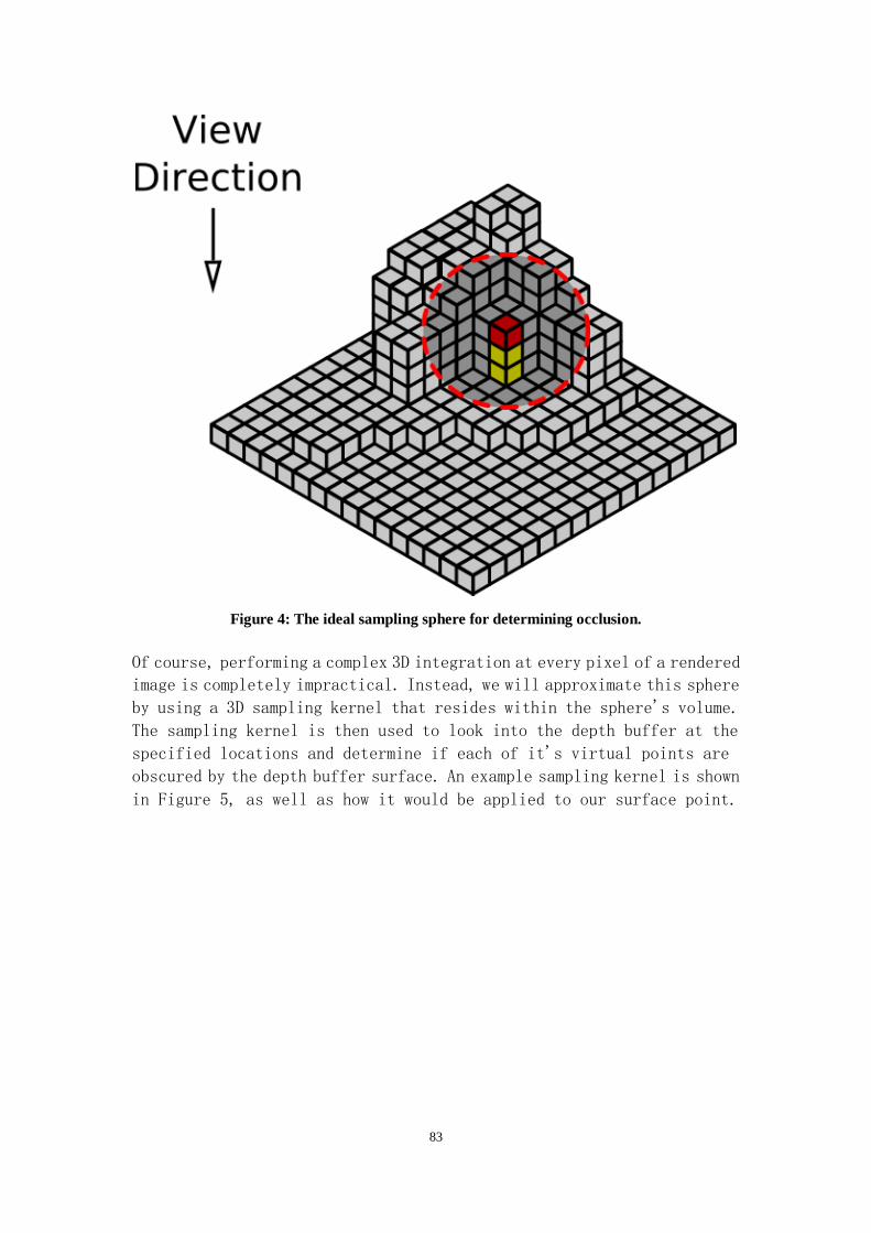
83

Figure 4: The ideal sampling sphere for determining occlusion.

Of course, performing a complex 3D integration at every pixel of a rendered

image is completely impractical. Instead, we will approximate this sphere

by using a 3D sampling kernel that resides within the sphere's volume.

The sampling kernel is then used to look into the depth buffer at the

specified locations and determine if each of it's virtual points are

obscured by the depth buffer surface. An example sampling kernel is shown

in Figure 5, as well as how it would be applied to our surface point.

84

Figure 5: Simplified sampling kernel and its position on the depth buffer.

The occlusion factor can then be calculated as the sum of the sampling

kernel point's individual occlusions. As you will see in the

implementation section, these individual calculations can be made more

or less sensitive based on several different factors, such as distance

from the camera, the distance between our point and the occluding point,

and artist specified scaling factors.

Implementation

With a clear understanding of how the algorithm functions, we can now

discuss a working implementation. As discussed in the algorithm theory

section, we will need a source of scene depth information. For

simplicity's sake, we will use a separate floating point buffer to store

the depth data. A more efficient technique, although slightly more complex,

would utilize the z-buffer to acquire the scene depth. The following code

snippet shows how to create the floating point buffer, as well as the

render target and shader resource views that we will be binding it to the

pipeline with:

// Create the depth buffer

D3D10_TEXTURE2D_DESC desc;

ZeroMemory( &desc, sizeof( desc ) );

desc.Width = pBufferSurfaceDesc->Width;

desc.Height = pBufferSurfaceDesc->Height;

desc.MipLevels = 1;

85

desc.ArraySize = 1;

desc.Format = DXGI_FORMAT_R32_FLOAT;

desc.SampleDesc.Count = 1;

desc.Usage = D3D10_USAGE_DEFAULT;

desc.BindFlags = D3D10_BIND_RENDER_TARGET |

D3D10_BIND_SHADER_RESOURCE;

pd3dDevice->CreateTexture2D( &desc, NULL, &g_pDepthTex2D );

// Create the render target resource view

D3D10_RENDER_TARGET_VIEW_DESC rtDesc;

rtDesc.Format = desc.Format;

rtDesc.ViewDimension = D3D10_RTV_DIMENSION_TEXTURE2D;

rtDesc.Texture2D.MipSlice = 0;

pd3dDevice->CreateRenderTargetView( g_pDepthTex2D, &rtDesc,

&g_pDepthRTV );

// Create the shader-resource view

D3D10_SHADER_RESOURCE_VIEW_DESC srDesc;

srDesc.Format = desc.Format;

srDesc.ViewDimension = D3D10_SRV_DIMENSION_TEXTURE2D;

srDesc.Texture2D.MostDetailedMip = 0;

srDesc.Texture2D.MipLevels = 1;

pd3dDevice->CreateShaderResourceView( g_pDepthTex2D,

&srDesc, &g_pDepthSRV );

Once the depth information has been generated, the next step is to

calculate the occlusion factor at each pixel in the final scene. This

information will be stored in a second single component floating point

buffer. The code to create this buffer is very similar to the code used

to create the floating point depth buffer, so it is omitted for brevity.

Now that both buffers have been created, we can describe the details of

generating the information that will be stored in each of them. The depth

buffer will essentially store the view space depth value. The linear view

space depth is used instead of clip space depth to prevent any depth range

distortions caused by the perspective projection. The view space depth

is calculated by multiplying the incoming vertices by the worldview matrix.

The view space depth is then passed to the pixel shader as a single

component vertex attribute.

fragment VS( vertex IN )

{

86

fragment OUT;

// Output the clip space position

OUT.position = mul( float4(IN.position, 1), WVP );

// Calculate the view space position

float3 viewpos = mul( float4( IN.position, 1 ), WV ).xyz;

// Save the view space depth value

OUT.viewdepth = viewpos.z;

return OUT;

}

To store the depth values in the floating point buffer, we then scale the

value by the distance from the near to the far clipping planes in the pixel

shader. This produces a linear, normalized depth value in the range [0,1].

pixel PS( fragment IN )

{

pixel OUT;

// Scale depth by the view space range

float normDepth = IN.viewdepth / 100.0f;

// Output the scaled depth

OUT.color = float4( normDepth, normDepth, normDepth,

normDepth );

return OUT;

}

With the normalized depth information stored, we then bind the depth

buffer as a shader resource to generate the occlusion factor for each pixel

and store it in the occlusion buffer. The occlusion buffer generation is

initiated by rendering a single full screen quad. The vertices of the full

screen quad only have a single two-component attribute which specifies

the texture coordinates at each of its four corners corresponding to their

locations in the depth buffer. The vertex shader trivially passes these

parameters through to the pixel shader.

fragment VS( vertex IN )

{

fragment OUT;

87

OUT.position = float4( IN.position.x, IN.position.y, 0.0f,

1.0f );

OUT.tex = IN.tex;

return OUT;

}

The pixel shader starts out by defining the shape of the 3D sampling kernel

in an array of three component vectors. The lengths of the vectors are

varied in the range [0,1] to provide a small amount of variation in each

of the occlusion tests.

const float3 avKernel[8] =

{

normalize( float3( 1, 1, 1 ) ) * 0.125f,

normalize( float3( -1,-1,-1 ) ) * 0.250f,

normalize( float3( -1,-1, 1 ) ) * 0.375f,

normalize( float3( -1, 1,-1 ) ) * 0.500f,

normalize( float3( -1, 1 ,1 ) ) * 0.625f,

normalize( float3( 1,-1,-1 ) ) * 0.750f,

normalize( float3( 1,-1, 1 ) ) * 0.875f,

normalize( float3( 1, 1,-1 ) ) * 1.000f

};

Next, the pixel shader looks up a random vector to reflect the sampling

kernel around from a texture lookup. This provides a high degree of

variation in the sampling kernel used, which will allow us to use a smaller

number of occlusion tests to produce a high quality result. This

effectively "jitters" the depths used to calculate the occlusion, which

hides the fact that we are under-sampling the area around the current

pixel.

float3 random = VectorTexture.Sample( VectorSampler,

IN.tex.xy * 10.0f ).xyz;

random = random * 2.0f - 1.0f;

Now the pixel shader will calculate a scaling to apply to the sampling

kernel based on the depth of the current pixel. The pixel's depth value

is read from the depth buffer and expanded back into view space by

multiplying by the near to far clip plane distance. Then the scaling for

the x and y component of the sampling kernel are calculated as the desired

radius of the sampling kernel (in meters) divided by the pixel's depth

(in meters). This will scale the texture coordinates used to look up

individual samples. The z component scale is calculated by dividing the

88

desired kernel radius by the near to far plane distance. This allows all

depth comparisons to be performed in the normalized depth space that our

depth buffer is stored in.

float fRadius = vSSAOParams.y;

float fPixelDepth = DepthTexture.Sample( DepthSampler,

IN.tex.xy ).r;

float fDepth = fPixelDepth * vViewDimensions.z;

float3 vKernelScale = float3( fRadius / fDepth, fRadius /

fDepth, fRadius / vViewDimensions.z ) ;

With the kernel scaling calculated, the individual occlusion tests can

now be carried out. This is performed in a for loop which iterates over

each of the points in the sampling kernel. The current pixel's texture

coordinates are offset by the randomly reflected kernel vector's x and

y components and used to look up the depth at the new location. This depth

value is then offset by the kernel vector's z-component and compared to

the current pixel depth.

float fOcclusion = 0.0f;

for ( int j = 1; j < 3; j++ )

{

float3 random = VectorTexture.Sample( VectorSampler,

IN.tex.xy * ( 7.0f + (float)j ) ).xyz;

random = random * 2.0f - 1.0f;

for ( int i = 0; i < 8; i++ )

{

float3 vRotatedKernel = reflect( avKernel[i], random )

* vKernelScale;

float fSampleDepth =

DepthTexture.Sample( DepthSampler, vRotatedKernel.xy +

IN.tex.xy ).r;

float fDelta = max( fSampleDepth - fPixelDepth +

vRotatedKernel.z, 0 );

float fRange = abs( fDelta ) / ( vKernelScale.z *

vSSAOParams.z );

fOcclusion += lerp( fDelta * vSSAOParams.w,

vSSAOParams.x, saturate( fRange ) );

}

}

89

The delta depth value is then normalized by an application selectable

range value. This is intended to produce a factor to determine the relative

magnitude of the depth difference. This information can, in turn, be used

to adjust the influence of this particular occlusion test. For example,

if an object is in the foreground of a scene, and another object is

partially obscured behind it then you don't want to count a failed

occlusion test for the back object if the foreground object is the only

occluder. Otherwise the background object will show a shadow-like halo

around the edges of the foreground object. The implementation of this

scaling is to linearly interpolate between a scaled version of the delta

value and a default value, with the interpolation amount based on the range

value.

fOcclusion += lerp( ( fDelta * vSSAOParams.w ), vSSAOParams.x,

saturate( fRange ) );

The final step before emitting the final pixel color is to calculate an

average occlusion value from all of the kernel samples, and then use that

value to interpolate between a maximum and minimum occlusion value. This

final interpolation compresses the dynamic range of the occlusion and

provides a somewhat smoother output. It should also be noted that in this

chapter’s demo program, only sixteen samples are used to calculate the

current occlusion. If a larger number of samples are used, then the

occlusion buffer output can be made smoother. This is a good place to scale

the performance and quality of the algorithm for different hardware

levels.

OUT.color = fOcclusion / ( 2.0f * 8.0f );

// Range remapping

OUT.color = lerp( 0.1f, 0.6, saturate( OUT.color.x ) );

With the occlusion buffer generated, it is bound as a shader resource to

be used during the final rendering pass. The rendered geometry simply has

to calculate it's screen space texture coordinates, sample the occlusion

buffer, and modulate the ambient term by that value. The sample file

provided performs a simple five sample average, but more sophisticated

filtering like a Gaussian blur could easily be used instead.

SSAO Demo

Demo Download: SSAO_Demo

The demo program developed for this chapter provides a simple rendering

http://wiki.gamedev.net/images/4/4d/SSAO_Demo.zip

90

of a series of cube models that is shaded only with our screen space ambient

occlusion. The adjustable parameters discussed for this technique can be

changed in real-time with the onscreen slider controls. Figure 6 below

shows the occlusion buffer and the resulting final output rendering.

Notice that the occlusion parameters have been adjusted to exaggerate the

occlusion effect.

Figure 6: A sample ambient occlusion buffer from the demo program.

91

Figure 7: The final output rendering from the demo program.

Conclusion

In this chapter we developed an efficient, screen space technique for

adding realism to the ambient lighting term of the standard phong lighting

model. This technique provides one implementation of the SSAO algorithm,

but it is certainly not the only one. The current method can be modified

for a given type of scene, with more or less occlusion for distant geometry.

In addition, the minimum and maximum amounts of occlusion, interpolation

techniques, and sampling kernels are all potential areas for improvement

or simplification. This chapter has attempted to provide you with an

insight into the inner workings of the SSAO technique as well as a sample

implementation to get you started.

Single Pass Environment Mapping

Introduction

Another technique for increasing the realism of a computer generated image

is to take into account an object's surroundings when rendering it. For

example, when rendering an object with a mirrored surface you must use

92

the object's surroundings to calculate the correct color at each pixel

that the object covers. In ray tracing, this is quite literally the case

where rays are reflected off of a particular surface to see what other

objects are visible in the reflected image.

However, as you may know ray tracing is typically a very computationally

and memory intensive process which is not easily implemented for use in

real-time rendering. However, as is always the case there are certain

assumptions and simplifications that can be made to allow a similar

algorithm to approximate a ray tracing technique. This chapter will focus

on one class of algorithms that attempt to do just this: environment

mapping.

Environment mapping utilizes an image buffer to store the appearance

information of all the objects surrounding one particular point in the

scene. Then, when rendering the desired reflective object, this buffer

is used to look up the color of the object that would be visible in the

reflection of the mirrored surface for each pixel. This reduces the

per-pixel rendering procedure from tracing a ray through the scene to only

a texture lookup, at the additional cost of generating the environment

map before performing the final rendering pass.

The fact that all of the scene information is gathered around a particular

point is one of the primary simplifications that allow the algorithm to

operate significantly faster than ray tracing. This is, however, also a

potential source of problems with the algorithm. Since we are generating

the environment maps around a point, there are potential accuracy issues

with using those maps to represent all of the light surrounding a 3D

geometric object. In addition, the reflective object itself can't appear

in the environment map since it would completely envelop the simulation

point.

Many variants of environment mapping have been proposed to counteract

these limitations while still retaining some degree of the speed of the

algorithm, and this chapter will investigate three of these variants:

sphere mapped environment mapping, cube mapped environment mapping, and

dual-paraboloid environment mapping. All three of these techniques store

the scene information as viewed from a single point in world space. Each

of these techniques uses different parameterizations to store the scene

information with differing formats.

The three techniques presented in this chapter provide a trade-off between

memory usage, rendering speed, and visual quality. Cube mapping utilizes

a total of six 2D render targets to store the scene, while dual paraboloid

mapping uses only two, and sphere mapping uses only one. However, the

93

quality of each technique is also partially dependent on how the memory

is used. Deciding which technique is appropriate for a given situation

requires a careful comparison of each ones strength's and weaknesses. In

this chapter, we will explore each of these techniques, how to implement

them efficiently with Direct3D 10, and provide a demo program to

experiment with and modify.

Algorithm Theory

Each of the three variants of environment mapping that we will investigate

require a method of generating the environment map as well as a method

of accessing the map once it is created. The key to understanding and

implementing these two procedures is to understand the parameterization

that is used to convert scene geometry to a form that can be stored in

a render target. For all of these methods, the parameterization is based

around defining a point that the environment map is surrounding. For the

following discussion we will name this point C. Point C is typically

located at the center of the object that will be rendered with the

reflective material to give the best approximation of the current

environment.

Sphere Mapping Parameterization

The simplest of these three parameterization techniques is called sphere

mapping. It uses a single 2D render target to represent the environment

surrounding point C. During the generation of the sphere map, the input

geometry is converted from world-space Cartesian coordinates to a new

coordinate system that represents how the geometry would look if we were

to view the scene by looking directly at a perfectly reflective sphere.

Once this conversion has been performed, each world space vertex position

will have been transformed to a new set of 3D coordinates. The x and y

coordinates identify the x and y locations on the reflecting sphere where

the corresponding vertex would appear when viewed from the current camera

location. You can picture the reflective sphere as being centered in the

render target, making the range of valid x and y coordinates [-1,1]. The

z coordinate simply represents the distance from point C to that vertex.

This parameterization essentially uses these new coordinates to determine

where in the environment map each vertex should be placed during the

creation of the map. This is shown in the following figure:

94

Figure 1: How spherical coordinates relate to a 2D texture buffer.

While the location that the vertex will reside in the environment map is

determined by the x and y coordinates, the z coordinate specifies the

distance from point C to that vertex. By using this depth information in

the output vertex position, the depth sorting hardware of the GPU (i.e.

the z-buffer) will automatically determine what object is the closest to

point C. This makes sense if you consider what each texel in the output

buffer represents. Each texel can be thought of as the color that would

be seen if you traced a ray from the viewer to point C, and then outward

in the direction that the sphere would reflect it to. This implicitly

requires that the closest object to point C is seen at that texel.

The mathematics of making the conversion from world space vertex positions

to sphere map locations are based on the concept of viewing a reflective

sphere. If you consider the output space of the vertex/geometry shaders,

also known as clip space, there is a range of [-1,1] for the x and y

coordinates and a range of [0,1] for the z coordinate. We need to find

an algorithm for filling this output space with the sphere map data while

utilizing as much of the available volume as possible.

To do this, we will consider the reflective sphere to be positioned at

the origin and have unit size. This effectively makes the sphere touch

the clip space boundary in the x and y directions at both the positive

and negative sides. This also means that the z-values of the sphere will

be in the [-1,1] range, but we will artificially set the z coordinate based

on the normalized distance from point C which will produce the required

[0,1] z range.

95

Let’s assume for now that point C is at the origin of world space. This

means that point C is located right in the center of the unit sphere. Now

consider a single vertex of the geometry in the environment surrounding

point C. To find the location on the unit sphere’s surface where that

vertex would be visible to point C, we simply normalize the vector

representing that vertex’s position (this works because point C is at

the origin). This vector represents the direction of the viewing ray that

would be reflected by the unit sphere. From the initial description of

the sphere mapping parameterization, we know that the view is coming from

a single direction, and is reflected in all directions by the unit sphere.

This is shown in the following figure:

Figure 2: How a sphere reflects a view to the surrounding environment.

Since we know the incident view vector is always in the same direction,

along the positive z-axis, then we now know the incident and reflected

vectors for this particular vertex. If a photon were to originate at the

vertex and travel to the sphere, then reflect off of the sphere towards

the viewer, then the direction of that reflected photon would be the

opposite of the view vector – which means it would be along the negative

z-axis.

Given these two vectors, we can solve for the normal vector on the unit

sphere’s surface that would have generated this reflection. Both the

96

incident and reflected vectors are unit length, so the vector between them

can be found by adding the two vectors, and then normalizing their size

by dividing by the resulting vector’s magnitude. Please note that both

of these vectors are defined as starting from Point C and travelling

outward - thus adding them and normalizing produces a vector between the

incident and reflected vectors. This process is shown in the following

equations:

With the normalized normal vector found, we simply take the x and y

coordinates of the normal vector to represent the x and y position in clip

space that this vertex will be placed at. You can visualize this as

projecting the normal vector onto the z = 0 plane in clip space. The output

z coordinate is found by calculating the distance from the origin to the

original vertex world space location. With these three pieces of

information, we can consider the vertex to be transformed into the sphere

map, and repeat the process for all remaining vertices in the surrounding

environment. A sample sphere map is shown here for your reference:

97

Figure 3: A sample sphere map generated by the demo for this chapter.

Once the environment map has been generated, the object that point C is

representing can be rendered as normal. A view vector is created from the

camera point to the current pixel, and is reflected about the normal vector

of the object's surface at the current pixel. After the vector has been

reflected, its direction can be converted to sphere map coordinates in

the same manner that was used to generate the map. These coordinates are

then used to sample the sphere map and determine what color the output

pixel should be.

The sphere mapping parameterization is relatively simple, but suffers

from a singularity point at the far side of the sphere with respect to

the viewer. This is due to the fact that there are many paths to the far

side of the sphere, but only one point to represent the endpoint of all

of these paths. In essence, the entire outer ring of the sphere map maps

to the single point on the far side of the sphere. This results in a

stretching artifact in the sphere map around the local area of the

singularity point.

98

This also means that each texel of the sphere map does not correspond to

the same amount of surface area when looking out at the environment from

point C. Since the reflective object will likely use most of the sphere

map at some location of its surface, the clarity of the reflected

environment will vary depending on where the sample falls within the

sphere map. This has the potential effect of distorting the object’s

surface appearance unevenly.

One other caveat with sphere mapping involves the scene geometry location

with respect to the singularity point. With one point representing

multiple path ways to that point, it is possible for a single small

triangle to be transformed to a much larger size in the sphere map if its

vertices happen to surround the singularity. This occurs because the

triangle is a linear object that is being warped into this spherical space.

If the triangle were to be subdivided many times, the resulting triangles

would appear along the outer rim of the sphere map instead of covering

a large portion of it. This issue can be overcome (either by detecting

the triangles that cross the singularity and removing them or ensuring

that there are no triangles there to begin with) but introduces a

limitation on the uses of this technique.

Cube Mapping Parameterization

Cube mapping is another parameterization that improves on sphere mapping.

The overall concept is that instead of representing the surrounding scene

with a spherical coordinate space you would use the 3D vector pointing

out from point C to intersect a cube instead of a sphere. This is shown

in the following figure:

Figure 4: A visualization of a cube map, and how it unfolds to individual render targets.

99

Each face of the cube is a 2D surface, which is easily accommodated with

standard rendering techniques. The procedure for generating a cube map

is simply to render the scene into each of the six faces of a cube with

the proper projection, and then use the reflected view vector to look up

the environment color in the appropriate cube face. Since a 3D reflection

vector is used, there are no strange conversions to new non-linear

coordinate spaces. Due to the popularity of this technique, there are even

special hardware instructions available that select the appropriate cube

face and sampling location, making this parameterization very easy to

implement.

There are several significant differences to note between sphere mapping

and cube mapping. The first is that cube mapping requires six rendering

passes, one for each cube face, to generate the environment map. This is

a significant increase in rendering workload that must be taken into

consideration. Also, similarly to sphere mapping, the texel to

environment surface area ratios are not uniform across each of the cube

faces. However, the ratio is significantly more stable than sphere mapping

and there are no singularity points – all areas of the environment can

be relatively accurately represented without any special case

considerations. Cube mapping thus offers higher image quality at the

expense of additional rendering complexity.

Even though there is additional rendering complexity, we will see in the

implementation section how to utilize several interesting techniques for

reducing the rendering cost of this parameterization that have only

recently been available with the introduction Direct3D 10.

Dual Paraboloid Parameterization

The two previous parameterization techniques both have different

advantages as well as disadvantages. Sphere mapping is simple and

efficient to implement, and yet it has certain image quality limitations.

Cube mapping provides better image quality at the expense of additional

rendering complexity. Now we will look at a third parameterization,

dual-paraboloid mapping, which attempts to blend the attributes of the

previous two techniques.

The concept behind dual paraboloid mapping is to use two opposing

paraboloid surfaces as the basis for the parameterization of the

environment instead of a sphere as used in sphere mapping. A paraboloid

is the surface that you would create if you were to revolve a parabola

about an axis that passes through its center point perpendicular to any

tangent vector at that point.

100

If you imagine looking at the cone side of a mirrored surface paraboloid,

then your view would reflect off of the surface of the paraboloid over

one hemisphere of the volume surrounding it. If you consider a second

paraboloid positioned in the opposite orientation to the first one, then

it would cover the other hemisphere surrounding point C. This is

illustrated in Figure 5:

Figure 5: A visualization of how two paraboloids reflect the environment in two directions.

Thus with two paraboloid surface elements we can describe the entire

environment surrounding point C. In this case, the two surface elements

are represented by two 2D render targets. The parameterization uses the

same methodology as sphere mapping to perform the conversion from

world/view space to the paraboloid space – by finding the normal vector

that would reflect the view vector to a particular location in the

surrounding environment. However, the mathematics of how to determine

normal vector are somewhat different for the paraboloid than it is for

the sphere.

To find the normal vector of the paraboloid we first need to consider the

mathematic construct that represents the paraboloid. We will use the

following equation to define the shape of the paraboloid:

101

Now we will define a point on the surface of the paraboloid as follows:

A common technique for finding a normal vector on a given surface is to

find two tangent vectors at the desired point and then take the cross

product of those vectors. To do this, we can evaluate the partial

derivatives for our point equation above:

Another way to find the normal vector is to consider the incident and

reflected vectors again. If both vectors are normalized (or at least the

same length), we can simply add them and the resulting vector has the same

direction as the normal vector. The reflection vector is opposite for the

two paraboloids since they are reflecting the scene into two opposite

directions. Regardless of the reflection vector direction, we can perform

the following equality to find the normal vector:

Once the sum of the incident and reflected vectors is known, we can

trivially find the normal vector by dividing the entire vector by its z

component:

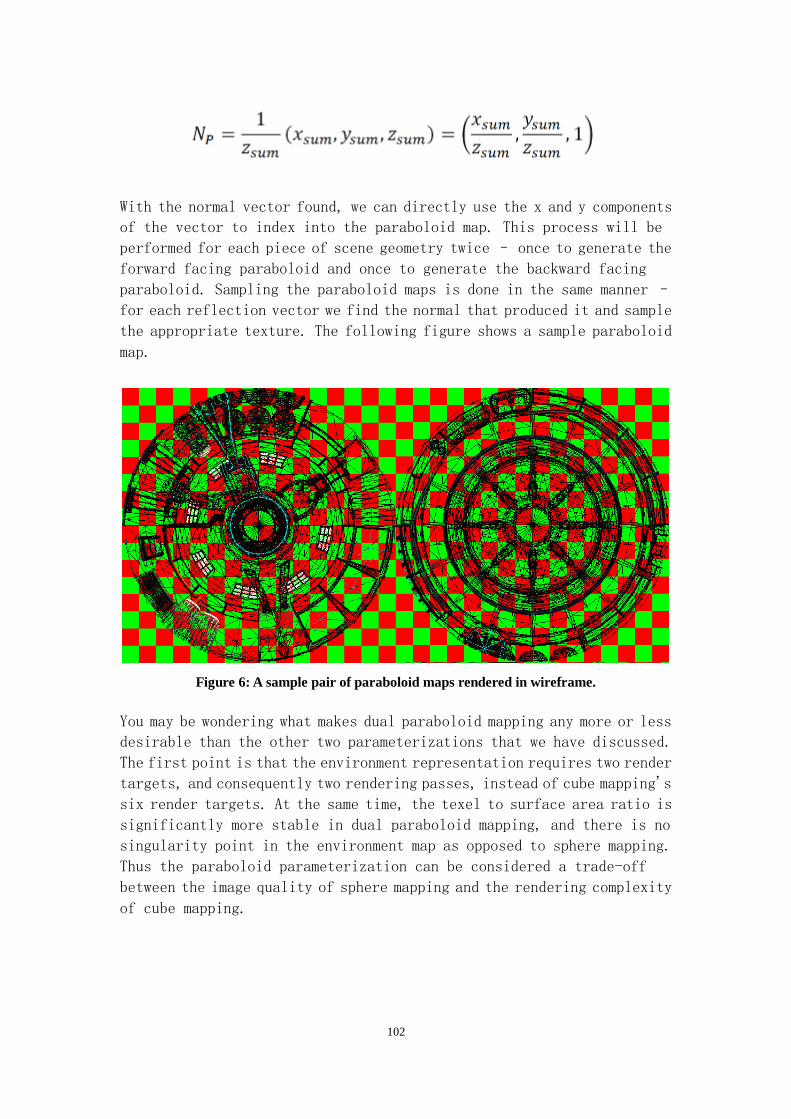
102

With the normal vector found, we can directly use the x and y components

of the vector to index into the paraboloid map. This process will be

performed for each piece of scene geometry twice – once to generate the

forward facing paraboloid and once to generate the backward facing

paraboloid. Sampling the paraboloid maps is done in the same manner –

for each reflection vector we find the normal that produced it and sample

the appropriate texture. The following figure shows a sample paraboloid

map.

Figure 6: A sample pair of paraboloid maps rendered in wireframe.

You may be wondering what makes dual paraboloid mapping any more or less

desirable than the other two parameterizations that we have discussed.

The first point is that the environment representation requires two render

targets, and consequently two rendering passes, instead of cube mapping's

six render targets. At the same time, the texel to surface area ratio is

significantly more stable in dual paraboloid mapping, and there is no

singularity point in the environment map as opposed to sphere mapping.

Thus the paraboloid parameterization can be considered a trade-off

between the image quality of sphere mapping and the rendering complexity

of cube mapping.

103

Implementation

With a solid understanding of the theory behind each of these

parameterizations, we can now investigate how to implement them while

utilizing some of the unique new features available in Direct3D 10. We

will look at the implementation of the sphere, cube, and paraboloid

parameterizations in turn, including the resources required and the

rendering sequences used.

Sphere Mapping Implementation

As we have discussed above, sphere mapping utilizes a single 2D render

target. Thus the render target and the depth target used to generate the

sphere map can be created in the same manner as normal.

// Create depth stencil texture.

dstex.Width = ENVMAPSIZE;

dstex.Height = ENVMAPSIZE;

dstex.MipLevels = 1;

dstex.ArraySize = 1;

dstex.SampleDesc.Count = 1;

dstex.SampleDesc.Quality = 0;

dstex.Format = DXGI_FORMAT_D32_FLOAT;

dstex.Usage = D3D10_USAGE_DEFAULT;

dstex.BindFlags = D3D10_BIND_DEPTH_STENCIL;

dstex.CPUAccessFlags = 0;

dstex.MiscFlags = 0;

V_RETURN( pd3dDevice->CreateTexture2D( &dstex, NULL,

&g_pSphereEnvDepthMap ));

// Create the sphere map render target

dstex.Format = DXGI_FORMAT_R8G8B8A8_UNORM;

dstex.MipLevels = MIPLEVELS;


dstex.BindFlags = D3D10_BIND_RENDER_TARGET |


dstex.MiscFlags = D3D10_RESOURCE_MISC_GENERATE_MIPS;


&g_pSphereEnvMap ));

104

With the render and depth targets created, we can also create the resource

views that we will need to connect them to the rendering pipeline. The

depth target will require only a depth stencil view, while the render

target will require both a render target view as well as a shader resource

view. This is also shown in the bind flags used to create the respective

resources.

// Create the depth stencil view for the sphere map

DescDS.Format = DXGI_FORMAT_D32_FLOAT;

DescDS.ViewDimension = D3D10_DSV_DIMENSION_TEXTURE2D;

DescDS.Texture2D.MipSlice = 0;

V_RETURN( pd3dDevice->CreateDepthStencilView( g_pSphereEn

vDepthMap, &DescDS, &g_pSphereEnvDepthMapDSV ));

// Create the render target view for the sphere map

DescRT.Format = DXGI_FORMAT_R8G8B8A8_UNORM;

DescRT.ViewDimension = D3D10_RTV_DIMENSION_TEXTURE2D;

DescRT.Texture2D.MipSlice = 0;

V_RETURN( pd3dDevice->CreateRenderTargetView( g_pSphereEn

vMap, &DescRT, &g_pSphereEnvMapRTV ));

// Create the shader resource view for the sphere map

ZeroMemory( &SRVDesc, sizeof(SRVDesc) );

SRVDesc.Format = DXGI_FORMAT_R8G8B8A8_UNORM;

SRVDesc.ViewDimension = D3D10_SRV_DIMENSION_TEXTURE2D;

SRVDesc.Texture2D.MipLevels = MIPLEVELS;

V_RETURN( pd3dDevice->CreateShaderResourceView( g_pSphere

EnvMap, &SRVDesc, &g_pSphereEnvMapSRV ));

Once the resources are created, we can turn our attention to generating

the sphere map for use in the subsequent final rendering pass. This

particular implementation utilizes all three programmable shader stages

in the Direct3D 10 pipeline. To begin with, the vertex shader will

transform all of the incoming geometry into a ‘view’ space in which the

viewer is actually located at point C. This has the advantage that it

places point C at the origin of this space, making the transformations

required further down the pipeline simpler (you will see in the geometry

shader how this helps). The texture coordinates of each vertex are simply

105

passed through to the output structure. The vertex shader listing is shown

here:

GS_ENVMAP_IN VS_SphereMap( VS_ENVMAP_IN input )

{

GS_ENVMAP_IN output = (GS_ENVMAP_IN)0.0f;

// Compute world position

float4 PosWS = mul( input.Pos, mWorld );

// Compute view position

float4 PosVS = mul( PosWS, g_mViewCM[0] );

// Output the view space position

output.Pos = PosVS;

// Propagate tex coord

output.Tex = input.Tex;

return output;

}

The bulk of the work in generating the sphere map occurs in the geometry

shader. The geometry shader will iterate over the three vertices of the

current triangle being rendered into the sphere map as shown here:

// Compute sphere map coordinates for each vertex

for( int v = 0; v < 3; v++ )

{

.....

.....

}

For each of these vertices, we begin by finding a unit length vector from

point C to the vertex. Since the incoming vertices were transformed to

view space in the vertex shader, we can simply normalize the input vertex

position to obtain the vector.

// Find the normalized direction to the vertex

float3 SpherePos = normalize( input[v].Pos.xyz );

Next, we will add the view vector to the position vector to obtain the

un-normalized normal vector of the sphere. Then we normalize the result

to produce a normal vector that resides within the unit sphere.

106

// Add the view direction vector --> always (0,0,-1)

// This produces a vector in the same direction as the

// normal vector between the incident & reflected

SpherePos.z -= 1;

// Re-normalize the vector for unit length

SpherePos = normalize( SpherePos );

This normal vector provides the x and y coordinates for the output clip

space position of the vertex. The z coordinate is found by calculating

the distance from point C to the view space position of the vertex, and

there is no perspective warping so the w coordinate can safely be set to

1.

// Output the x,y coordinates of the normal to locate

// the vertices in clip space

output.Pos.x = SpherePos.x;

output.Pos.y = SpherePos.y;

// Output the view space distance from point C to vertex

output.Pos.z = length( input[v].Pos.xyz ) / 100.0f;

// There is no perspective warping, so w = 1

output.Pos.w = 1;

The input texture coordinates are simply passed through to the pixel

shader, and then the vertex is appended to the output stream.

// Propagate the texture coordinates to the pixel shader

output.Tex = input[v].Tex;

CubeMapStream.Append( output );

The pixel shader only samples the object’s texture to place the

appropriate color into the sphere map where the geometry shader positioned

it.

The second half of the sphere map algorithm is to be able to access the

appropriate location in the sphere map when rendering the final scene.

This is performed primarily in the pixel shader, while the vertex shader

and geometry shader are only used for vertex transformation and normal

vector setup. While accessing the sphere map, we initially have the world

space surface normal vector of the object being rendered. We also have

the current pixel location in world space as well as the view position

107

– which allows us to create the view vector. Together with the normal

vector we can then create the reflected view vector, which indicates the

direction in the scene that we wish to find in the sphere map.

// Vector from eye to pixel in WS

float3 I = vin.wPos.xyz - vEye;

// Reflected eye vector in WS

float3 wR = I - 2.0f * dot( I, wN ) * wN;

The first task is to convert the reflected view vector to the same view

space that was used while generating the sphere map.

// Reflected eye vector in front paraboloid basis

float3 wRf = normalize( mul( wR, (float3x3)g_mViewCM[0] ) );

With this reflection vector in the correct view space, we can follow the

same process that we did in generating the sphere map – find the normal

vector that would reflect the view vector in the direction of the

reflection vector. We do this by adding the view vector and renormalizing

the resulting vector.

// Add the view vector to the reflected vector

wRf.z -= 1.0f;

// Re-normalize the length of the resulting vector

float size = length( wRf.xyz );

wRf.x = wRf.x / size;

wRf.y = wRf.y / size;

These coordinates are now in the same clip space that we discussed earlier

– meaning that the x and y coordinates are in the range of [-1,1]. Since

we are now accessing a texture, we need to map these coordinates into

texture space, with the x range of [0,1] and the y range of [0,1] with

the origin at the top left corner of the texture.

// Remap the coordinates to texture space

float2 coords;

coords.x = ( wRf.x / 2 ) + 0.5;

coords.y = 1 - ( ( wRf.y / 2 ) + 0.5);

Finally, we sample the sphere map with a standard 2D texture sampler.

// Sample the sphere map

108

float4 SphereSampleFront = g_txSphereMap.Sample( g_samLinear,

coords );

This value can then be directly used or blended with other parameters to

appear partially reflective.

Cube Mapping Implementation

Next we will investigate the cube mapping implementation. The cube map

resources are significantly different than the resources that we created

for sphere mapping. First we will look at the creation of the render and

depth targets.

// Create cubic depth stencil texture

D3D10_TEXTURE2D_DESC dstex;











dstex.MiscFlags = D3D10_RESOURCE_MISC_TEXTURECUBE;


&g_pCubeEnvDepthMap ));

// Create the cube map for env map render target




dstex.MiscFlags = D3D10_RESOURCE_MISC_GENERATE_MIPS |

D3D10_RESOURCE_MISC_TEXTURECUBE;



&g_pCubeEnvMap ));

The cube map resources make use of one of the new features in Direct3D

10 – texture arrays. The idea here is to create a single resource that

is interpreted as multiple individual textures. These can then be

109

individually indexed within one of the programmable shader stages in the

rendering pipeline. In addition to being able to access the textures

individually, you can also bind the texture array to the pipeline as a

render target. Then each primitive can specify a system value in its output

structure (identified with the semantic SV_RenderTargetArrayIndex) that

will determine which texture in the array will receive that particular

primitive. Consider what techniques this ability can allow – this

provides a significant freedom for sorting or multiplying geometric data.

In this case, we will be using six textures in the texture array – one

for each of the six directions in the cube map. This is specified with

the dstex.ArraySize parameter, which we have set to six. Another point

of interest is the dstex.MiscFlags parameter. In both the render and depth

targets we specify the D3D10_RESOURCE_MISC_TEXTURECUBE flag. This allows

the texture array resource to be bound to the rendering pipeline as a cube

texture instead of just a simple texture array. With a cube texture, we

can utilize the hardware instructions specifically added for accessing

cube maps. We’ll see how to utilize these instructions later on in this

section. Next we create the resource views needed for binding the render

and depth targets to the pipeline.

// Create the depth stencil view for the entire cube

D3D10_DEPTH_STENCIL_VIEW_DESC DescDS;


DescDS.ViewDimension = D3D10_DSV_DIMENSION_TEXTURE2DARRAY;

DescDS.Texture2DArray.FirstArraySlice = 0;

DescDS.Texture2DArray.ArraySize = 6;

DescDS.Texture2DArray.MipSlice = 0;

V_RETURN( pd3dDevice->CreateDepthStencilView( g_pCubeEnvD

epthMap, &DescDS, &g_pCubeEnvDepthMapDSV ));

// Create the 6-face render target view

D3D10_RENDER_TARGET_VIEW_DESC DescRT;

DescRT.Format = dstex.Format;

DescRT.ViewDimension = D3D10_RTV_DIMENSION_TEXTURE2DARRAY;

DescRT.Texture2DArray.FirstArraySlice = 0;

DescRT.Texture2DArray.ArraySize = 6;

DescRT.Texture2DArray.MipSlice = 0;

V_RETURN( pd3dDevice->CreateRenderTargetView( g_pCubeEnvM

ap, &DescRT, &g_pCubeEnvMapRTV ));

// Create the shader resource view for the cubic env map

110

D3D10_SHADER_RESOURCE_VIEW_DESC SRVDesc;


SRVDesc.Format = dstex.Format;

SRVDesc.ViewDimension = D3D10_SRV_DIMENSION_TEXTURECUBE;

SRVDesc.TextureCube.MipLevels = MIPLEVELS;

SRVDesc.TextureCube.MostDetailedMip = 0;

V_RETURN( pd3dDevice->CreateShaderResourceView( g_pCubeEn

vMap, &SRVDesc, &g_pCubeEnvMapSRV ));

Here again, we specify that we will be using these resources as a cube

texture. The ViewDimension parameter specifies the actual usage for each

of the resource views. Notice that the depth target and render target views

specify D3D10_DSV_DIMENSION_TEXTURE2DARRAY and

D3D10_RTV_DIMENSION_TEXTURE2DARRAY while the shader resource view

specifies D3D10_SRV_DIMENSION_TEXTURECUBE. This is because while we are

generating the cube map we want to interpret the resources as texture

arrays and while we are accessing the cube map we want to interpret the

resources as a cube texture. Prior to Direct3D 10, this type of multiple

interpretations were not possible!

With the resources ready to go, we can start the algorithm by generating

the cube map. In pre-Direct3D 10 implementations, we would need to render

the geometry of the scene into each face of the cube map manually. However,

with the texture array resource we can render the geometry once and then

multiply the data in the geometry shader – producing one copy of the

geometry for each of the six cube faces. To get started, the vertex shader

is used to convert the input object space geometry to world space.

// Compute world position

output.Pos = mul( input.Pos, mWorld );

Next, the geometry shader receives the world space geometry one primitive

at a time. For each primitive, the geometry shader iterates over it six

times and transforming it into the appropriate viewing space for each of

the cube faces. This is shown in the following code listing.

for( int f = 0; f < 6; ++f )

{

// Compute screen coordinates

PS_ENVMAP_IN output;

output.RTIndex = f;

for( int v = 0; v < 3; v++ )

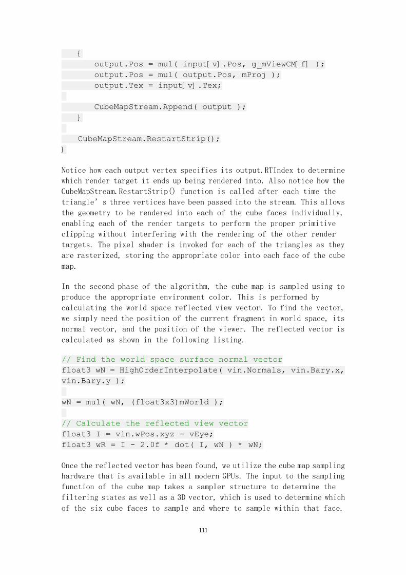
111

{

output.Pos = mul( input[v].Pos, g_mViewCM[f] );

output.Pos = mul( output.Pos, mProj );



}

CubeMapStream.RestartStrip();

}

Notice how each output vertex specifies its output.RTIndex to determine

which render target it ends up being rendered into. Also notice how the

CubeMapStream.RestartStrip() function is called after each time the

triangle’s three vertices have been passed into the stream. This allows

the geometry to be rendered into each of the cube faces individually,

enabling each of the render targets to perform the proper primitive

clipping without interfering with the rendering of the other render

targets. The pixel shader is invoked for each of the triangles as they

are rasterized, storing the appropriate color into each face of the cube

map.

In the second phase of the algorithm, the cube map is sampled using to

produce the appropriate environment color. This is performed by

calculating the world space reflected view vector. To find the vector,

we simply need the position of the current fragment in world space, its

normal vector, and the position of the viewer. The reflected vector is

calculated as shown in the following listing.

// Find the world space surface normal vector

float3 wN = HighOrderInterpolate( vin.Normals, vin.Bary.x,

vin.Bary.y );

wN = mul( wN, (float3x3)mWorld );

// Calculate the reflected view vector



Once the reflected vector has been found, we utilize the cube map sampling

hardware that is available in all modern GPUs. The input to the sampling

function of the cube map takes a sampler structure to determine the

filtering states as well as a 3D vector, which is used to determine which

of the six cube faces to sample and where to sample within that face.

112

// Sample the cube map

float4 CubeSample = g_txEnvMap.Sample( g_samCube, wR );

This output color represents the environment color that the viewer would

see on the reflective object.

Dual Paraboloid Implementation

The final parameterization that we will implement is the dual paraboloid

parameterization. The dual paraboloid environment map will also use a

texture array as its resource, but will use it somewhat differently than

the cube map parameterization. Here is the code listing to create the depth

and render targets for the dual paraboloid map.

// Create cubic depth stencil texture.











dstex.MiscFlags = 0;


&g_pParabEnvDepthMap ));

// Create the paraboloid map for env map render target






dstex.MiscFlags = D3D10_RESOURCE_MISC_GENERATE_MIPS;


&g_pParabEnvMap ));

If you recall the discussion of the paraboloid parameterization, we need

to create two 2D render targets. Thus, we will create a texture array with

113

two texture elements. However, as opposed to the creation of the cube map,

we do not specify the D3D10_RESOURCE_MISC_TEXTURECUBE miscellaneous flag

since we will not be using the cube texture hardware. The resource views

used to bind this resource to the pipeline are created next.

// Create the depth stencil view for the entire cube


DescDS.ViewDimension = D3D10_DSV_DIMENSION_TEXTURE2DARRAY;

DescDS.Texture2DArray.FirstArraySlice = 0;

DescDS.Texture2DArray.ArraySize = 2;

DescDS.Texture2DArray.MipSlice = 0;

V_RETURN( pd3dDevice->CreateDepthStencilView( g_pParabEnv

DepthMap, &DescDS, &g_pParabEnvDepthMapDSV ));

// Create the 6-face render target view

DescRT.Format = DXGI_FORMAT_R8G8B8A8_UNORM;





V_RETURN( pd3dDevice->CreateRenderTargetView( g_pParabEnv

Map, &DescRT, &g_pParabEnvMapRTV ));

// Create the shader resource view for the cubic env map


SRVDesc.Format = DXGI_FORMAT_R8G8B8A8_UNORM;

SRVDesc.ViewDimension =

D3D10_SRV_DIMENSION_TEXTURE2DARRAY;

SRVDesc.Texture2DArray.ArraySize = 2;

SRVDesc.Texture2DArray.MipLevels = MIPLEVELS;

V_RETURN( pd3dDevice->CreateShaderResourceView( g_pParabE

nvMap, &SRVDesc, &g_pParabEnvMapSRV ));

With the resources in hand, we can now begin generating the paraboloid

maps. The generation phase utilizes a similar technique to what the cube

map uses. At the outermost level, each triangle is multiplied twice –

once for each of the two paraboloid maps. Then, each vertex is transformed

into the view space of point C. An additional per-vertex parameter,

output.ZValue, is also added to the output structure which is the view

space z component. This value determines if the current vertex is in the

‘front’ paraboloid or if it should be in the ‘back’ paraboloid.

114

Next, the paraboloid coordinates are calculated by normalizing the view

space position, adding the view vector (which is always (0,0,1)) and then

dividing by the z component (please see the algorithm theory section for

further details). Finally, the output depth value is calculated as

distance from point C, with the sign of the view space z component. This

is needed to ensure that geometry from one half-space doesn’t interfere

with the geometry destined to appear in the other half-space.

for( int f = 0; f < 2; ++f )

{


PS_PARABMAP_IN output;

output.RTIndex = f;

for( int v = 0; v < 3; v++ )

{

// Transform the geometry into the appropriate view

space

output.Pos = mul( input[v].Pos, g_mViewCM[f+2] );

// Output the view space depth for determining

// which paraboloid this vertex is in

output.ZValue = output.Pos.z;

// Normalize the view space position to get its

direction

float L = length( output.Pos.xyz );

output.Pos.xyz = output.Pos.xyz / L;

// Add the view vector to the direction

output.Pos.z += 1;

// Divide by 'z' to generate paraboloid coordinates

output.Pos.x = output.Pos.x / output.Pos.z;

output.Pos.y = output.Pos.y / output.Pos.z;

// Set the depth value for proper depth sorting

output.Pos.z = L * sign(output.ZValue) / 500;



}

115


}

To access the paraboloid map, we follow a similar procedure as when we

created it. This occurs primarily in the pixel shader, as shown in the

following listing.

// Calculate the world space surface normal

float3 wN = HighOrderInterpolate( vin.Normals, vin.Bary.x,

vin.Bary.y );

wN = mul( wN, (float3x3)mWorld );

// Calculate the reflected view vector



// Calculate two versions of this vector - one for

// the 'front' paraboloid and one for the 'back' paraboloid

float3 wRf = normalize( mul( wR, (float3x3)g_mViewCM[2] ) );

float3 wRb = normalize( mul( wR, (float3x3)g_mViewCM[3] ) );

// Calculate the front paraboloid coordinates

float3 front;

front.x = ( wRf.x / ( 2*(1+wRf.z) ) ) + 0.5;

front.y = 1 - ( (wRf.y / ( 2*(1+wRf.z) ) ) + 0.5);

front.z = 0;

// Calculate the back paraboloid coordinates

float3 back;

back.x = ( wRb.x / ( 2*(1+wRb.z) ) ) + 0.5;

back.y = 1 - ( (wRb.y / ( 2*(1+wRb.z) ) ) + 0.5);

back.z = 1;

// Sample the paraboloid maps

float4 ParaboloidSampleFront =

g_txParabFront.Sample( g_samParaboloid, front );

float4 ParaboloidSampleBack =

g_txParabFront.Sample( g_samParaboloid, back );

float fLight = saturate( dot( skyDir, wN ) ) + 0.2f;

// Combine both paraboloid maps

float4 outCol = 0.3*vMaterialDiff*fLight +

1.5 * vMaterialSpec * max( ParaboloidSampleFront,

ParaboloidSampleBack );

116

outCol.a = vMaterialDiff.a;//preserve alpha

return outCol;

The access is performed by first calculating the world space surface

normal, reflecting the view vector, and transforming the reflected view

vector to both of the two paraboloids view spaces. Once this is complete,

we then divide the x and y coordinates by one plus the z component of the

reflected vector (which corresponds to the view vector plus the reflection

vector, and then dividing by the z component) and scale and bias the result

to access texture space. The resulting texture coordinates are used to

sample their respective paraboloid maps. In this case, we take the sum

of the two samples since the samplers are configured for a black border

color. Only one paraboloid map should have non-black results due to the

nature of the half-space divide between them. Similarly to cube and sphere

mapping, the final resulting color can be used directly or blended with

other rendering techniques for more advanced effects.

Demo and Algorithm Performance

Demo Download: Single_Pass_Environment_Mapping_Demo.zip

The implementation is based on the DirectX SDK sample named 'CubeMapGS'.

The demo has been simplified somewhat to only render a reflective sphere

with its surroundings rendered as they were originally. A set of three

radial buttons allow the user to choose the parameterization to use during

the interactive viewing of the scene.

The results reflect the performance and quality characteristics that were

discussed in the algorithm theory section. The quality of the environment

maps are best when using cube mapping, then paraboloid mapping, and

finally sphere mapping. However, the opposite order applies to rendering

speed – sphere mapping is the fastest, followed by paraboloid mapping

and then cube mapping. The percentage increases will vary from machine

to machine, but the speed change is approximately proportional to the

number of render targets used.

Improving Sphere Map Implementation

While working with the demo, you will notice two different negative

effects while using sphere mapping. The first effect is that the sphere

rendering has a large warping location at one point on its surface. This

point corresponds to the ‘singularity’ that was discussed in the sphere

http://wiki.gamedev.net/images/1/1a/Single_Pass_Environment_Mapping_Demo.zip

117

mapping theory section. If you click and drag around the sphere you can

rotate the scene from other angles that cannot see the singularity – hence

this issue can be overcome by updating the sphere map’s ‘view space’

that is used during the generation of the map. By continually shifting

the sphere map’s forward direction you can effectively hide the

singularity.

The second and more critical rendering artifact can be seen when the

scanner arm passes behind the singularity point. In this case, the scanner

arm is the closest object to point C, and will thus be rendered on top

of all of the other objects in the scene. Since it is passing through the

singularity point it should ideally be rendered as a ring around the

outermost portion of the sphere map, while the inner portion of the sphere

map should contain the rest of the environment that isn’t directly behind

the singularity point.

The problem here is that the scanner arm’s triangles are linearly

interpolated, and don’t take into account any form of wrapping around

the back of the cube map. The following figure shows this effect. On the

left hand side, the scanner arm is shown after being transformed to world

space. On the right hand side, you can see that there are many instances

of the geometry being wrapped around the sphere instead of around the

outside of the sphere.

Figure 7: Incorrect rasterization of a triangle on the front of the sphere.

This is not a simple problem to solve. The purely mathematic solution would

be to detect when there is a polygon overlapping the singularity, and then

dynamically tessellating the polygon to remove the area surrounding the

singularity. This is shown in the following figure.

118

Figure 8: A dynamically tessellated ‘hole’ in the triangle.

Due to the complexity of this type of operation, it is not the most

efficient to perform in a geometry shader. Another potential solution

would be to place the reflective object in such an orientation that there

are no polygons overlapping the singularity. In either case, care must

be taken while using sphere mapping to ensure that the artifacts are not

visible to the end user!

Improving Paraboloid Map Implementation

You may also notice artifacts in the paraboloid environment mapping demo

as well. The two paraboloids are positioned such that one of them is

pointing upward and the other is pointing downward. In the space where

the two paraboloids meet, you can see a thin black line separating the

two. This is also caused by the triangles being rasterized in a linear

space instead of the non-linear paraboloid interpolation. Consider the

following image of a paraboloid map:

119

Figure 9: A wireframe view of a paraboloid map showing the linear rasterization of triangles

(taken from the upward facing paraboloid in the demo program).

The linear points between the vertices of the outermost triangles cause

this line to appear between the paraboloids. In this case, we must also

dynamically detect when a triangle crosses the paraboloid boundary and

then dynamically tessellate those triangles until the resulting error

would be smaller than a single texel. I hope to include an implementation

of this dynamic tessellation in a future revision of the demo.

One other possibility is to choose a random axis to split the paraboloid

on. This would cause a small visual discontinuity in a random direction.

Then the results from the current frame and the previous frame could be

used together to remove the holes. Regardless of the technique used, this

issue must also be addressed to effectively use paraboloid mapping.

120

Conclusion

In this chapter, we have made a thorough investigation of sphere mapping,

cube mapping, and paraboloid mapping. After reviewing the theory behind

each technique, we have implemented each of them for an interactive demo

that can be used to compare their various properties. The correct choice

of a parameterization requires knowledge of the situations that it will

be used in. For cases that require high quality rendering, cube maps are

probably the technique to use. However, if rendering speed is the most

important consideration, then sphere mapping may be more appropriate. If

a good blend between the two makes more sense, then dual paraboloid mapping

would be a logical choice. In any of these three cases, environment mapping

should be within the reach of modern real-time rendering system.

Dynamic Particle Systems

Introduction

Particle systems have long served as a technique for implementing

environmentally based effects. A particle system consists of many

sub-elements (the particles) that when considered together (the system)

appear to represent a more complex entity. The particle system technique

provides a useful and intuitive method for rendering complex phenomena

by accumulating the results of many simple rendering operations. By using

a cumulative rendering process, the particle system provides a rough

simulation of a significantly more complex object with relatively low cost

rendering. They are commonly used for things like smoke, clouds, dust,

fire, rain, and snow.

However, even though particle systems can contribute to the general

impression of realism in a game world, they have historically been

restricted to graphical effects and have generally not been capable of

interacting with the player or other entities within the game world due

to the large number of particles that are normally used. Consider trying

to perform collision detection and response of 100,000 particles with all

of the objects in the game world – this would be extremely difficult to

implement in an efficient manner!

In this chapter, we will investigate how to implement a particle system

on the GPU that provides interaction with the objects inhabiting the game

world. This system will include the physical simulation of the particles

as well as the rendering process used to present the results of the

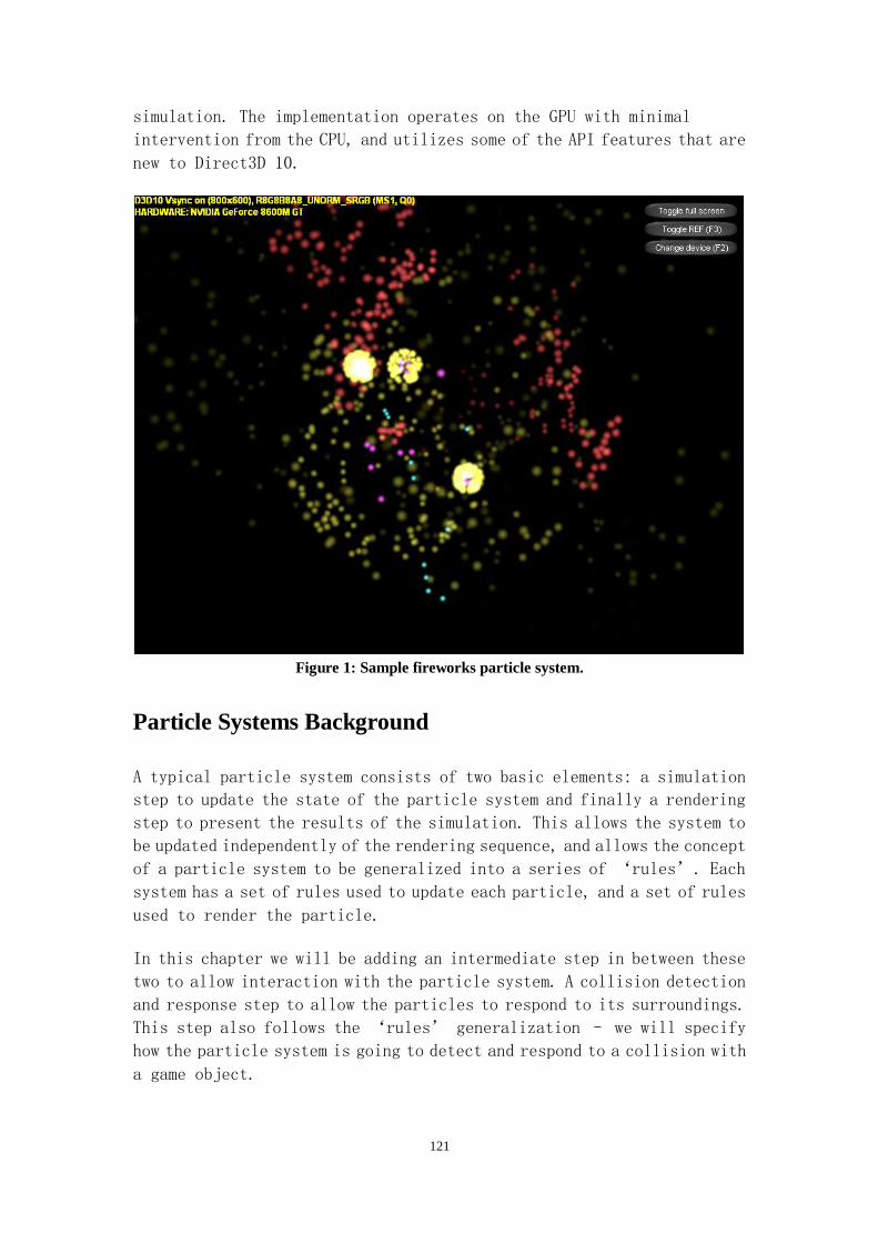
121

simulation. The implementation operates on the GPU with minimal

intervention from the CPU, and utilizes some of the API features that are

new to Direct3D 10.

Figure 1: Sample fireworks particle system.

Particle Systems Background

A typical particle system consists of two basic elements: a simulation

step to update the state of the particle system and finally a rendering

step to present the results of the simulation. This allows the system to

be updated independently of the rendering sequence, and allows the concept

of a particle system to be generalized into a series of ‘rules’. Each

system has a set of rules used to update each particle, and a set of rules

used to render the particle.

In this chapter we will be adding an intermediate step in between these

two to allow interaction with the particle system. A collision detection

and response step to allow the particles to respond to its surroundings.

This step also follows the ‘rules’ generalization – we will specify

how the particle system is going to detect and respond to a collision with

a game object.

122

Each particle in a particle system is normally represented by a single

point in world space. For every frame, the simulation phase updates the

position and velocity information of each particle according to the

simulation rules of the system being modeled. For example, in a smoke

particle system the particles will drift upward in a semi-uniform manner,

while a spark particle system would move the particles very quickly in

a small cone around the direction of the spark spray.

Once the particles have been updated, their new states are then used to

determine if any collisions have occurred between the previous time step

and the current time step. If a collision has occurred, then a collision

response can be applied to that particle. This collision detection and

response is used to model some physical properties of the phenomena that

the particle system is representing. An example of this would be the

difference between smoke wrapping around an object as opposed to a spark

bouncing off of an object and flying in the opposite direction. This could

also be specialized based on the object that the particle collides with

as well. For example, if a spark hits a wall it would bounce off, but if

it hits a bucket of water it would be extinguished and cease to exist.

Specialty state information specific to a given particle system can also

be stored and updated for each particle. Examples of this type of specialty

information could be an animation state, transparency levels, or particle

color. More sophisticated rendering techniques can be implemented using

these additional state data.

Once a particle has been updated, it is typically rendered as a more

complex primitive than a simple particle. A screen aligned quad (pair of

triangles as shown in Figure 2) with a suitable texture applied for the

given particle system is often used to provide additional complexity to

the system without incurring large rendering speed penalty. Of course,

this is not the only representation available - the particles could also

be rendered as individual particle primitives, more complex geometry, or

even animated meshes. However, most systems utilize the screen aligned

quads or some similar technique for rendering due to the large number of

renders that need to be performed. The expansion of particles into

textured quads is visualized in Figure 2.

123

Figure 2: Various particle representation: points, screen aligned quads, and textured quads.

When using screen aligned quads, the rules of the system for rendering

amount to designating a texture to be applied to them. This allows

flexibility for implementing different particle systems by simply

changing the texture used during the rendering process. For example, using

a sphere texture to simulate round particles or using a smoke puff texture

to simulate portions of a cloud or a smoke plume. Other potential rules

for rendering a particle system can include the use of transparency, depth

sorting, and various alpha blending modes to achieve special effects.

All of the example particle systems mentioned above (such as smoke systems

and spark systems) can be represented in the same framework by simply

changing the rules that are used to update the particle's state, how it

responds to collisions, and how it is rendered.

Implementation Difficulty

The main difficulty with implementing this type of interactive particle

system is the large amount of CPU processing that is required. For each

frame to be rendered, the CPU must iterate through an array of particles

and test each particle for collisions with other objects in the game world,

and then update the particle state accordingly. This type of operation

may seem suited to modern multi-core CPUs, and indeed they are. Each

particle can be updated independently of each other, making each particle

able to be updated in separate threads running on multiple processors in

isolation. However, modern CPUs typically are only dual or quad-core with

octo-core CPUs likely to come sometime in the future. Even if the particles

do not interact with any objects in the environment, the CPU would be

required to perform a significant number of operations every frame –

basically monopolizing the available processing time available for other

operations.

In contrast to a general purpose CPU's serialized performance in these

types of tasks, modern GPUs have been specially designed to perform

multiple similar computations at the same time on different data. Modern

124

GPUs can have several hundred simple processing elements on them, making

them very well suited to updating a particle system. This computational

model just happens to be precisely what is required to update a particle

system. With this in mind, if we move a particle system onto the GPU then

we could leverage its parallel processing power to create more attractive

and realistic effects that can be interactive with the game world.

GPU Based Particle Systems (D3D9)

In fact, this type of system has been implemented on the GPU with Direct3D

9 level hardware. The typical implementation uses a pair of render targets

to store particle state information. Each frame would render a full screen

quad and read the particle information from the render target in a pixel

shader texture read. That information was used to calculate the new state

of the particle, which was subsequently written to the second render

target. Then a set of four vertices is rendered for each pixel (usually

using instancing) to read the information from the render target and draw

the particle in the appropriate position on screen. Then, on the next frame,

the two render targets are swapped and the process is repeated. The

flowchart for this updating and rendering process is depicted in Figure

3 below.

125

Figure 3: Particle system using render targets for particle storage.

This technique does indeed work well and moves the computational load off

of the CPU and onto the GPU, but is somewhat limited with respect to

creating new particles or removing old ones from the system. Since the

particles are stored in a render target they can only be accessed through

a texture sampler or by manually locking and editing the render target

data, which can become a performance bottleneck. In addition, the amount

of information available to store per particle is limited to a single four

component vector unless multiple render targets are used. Finally, since

each pixel of a render target is considered a particle, it is necessary

to update all pixels of the render target with a full screen quad since

the CPU doesn't know how many of the particles are currently active. This

process can be optimized somewhat with a stencil pre-pass to eliminate

the unused pixels early on in the simulation step. The inactive pixels

can be culled away, but it still requires additional processing to

determine that they aren't active.

126

This era of particle systems have also used some forms of interactivity

as well [Latta04]. These typically used scene depth information to

approximate collision detection. This system is functional, but it would

be desirable to have a system that could produce collisions from any

direction around an object in the scene.

GPU Based Particle Systems (D3D10)

Even though D3D9 techniques were a huge improvement over CPU only particle

system, its utilization of a somewhat inefficient update mechanism and

its limited collision detection system limits the amount of work that can

be done during the processing of each particle. However, with D3D10

hardware we can use a more efficient method of storing/retrieving,

updating, and rendering the particles in our particle system.

The additional pipeline stages added in Direct3D 10, specifically the

geometry shader and the stream output stage, provide the tools to

implement an efficient technique to manage the lifetime of a particle.

Since the geometry shader and stream output stages work with vertex

information prior to the rasterization stage, the particle state

information can be stored as a vertex instead of a pixel/texel. This

provides the nice benefit that you can store as much per particle data

as can fit within a single vertex declaration, which is up to 16 four

component vectors per vertex! Figure 4 provides a flow chart demonstrating

how this updated technique operates.

Figure 4: Particle system using vertex buffers for particle storage.

127

With the efficient updating mechanism of this technique, additional work

can be performed during the particle update phase at a relatively low

performance penalty. In particular, it is possible to make the particle

system interact with the other objects that inhabit the game world in a

parametric form. This capability would add significantly to the realism

of the scene. For example, it would be feasible to have a smoke plume wrap

around an animated character or snow fall appropriately onto a landscape

entirely in real time on the GPU.

To demonstrate how to implement an interactive particle system, we will

extend one of the samples provided in the DirectX SDK. In the installation

directory of the DirectX SDK, there is a Direct3D 10 sample program named

ParticlesGS that demonstrates how to implement a fireworks particle

system using stream output and the geometry shader to control the update

and lifespan of each particle in the system.

The particles are represented as vertices in two vertex buffers which

alternate between frames as the source or destination vertex buffers. For

each particle system update, the current source vertex buffer is rendered

to the geometry shader, which then determines how to update each type of

particle. Once the vertex is updated, the geometry shader emits the

updated particle along with an appropriate number of new particles or if

the particle is considered 'dead' the geometry shader will not emit a new

vertex, effectively removing that particle from the system.

In this chapter, we will modify this sample to make the particles in the

system interact with a series of application specified and controlled

shapes. Multiple shape types can be supported in a single pass, while still

retaining operation entirely on the GPU with only CPU guidance. Figure

6 demonstrates the modified algorithm flow chart for the interactive

particle system.

128

Figure 5: Modified algorithm flow chart for this chapter's demo.

Algorithm Theory

To create an interactive particle system, we first need to define how we

will represent the world objects while performing collision detection

with the particle system. The most accurate solution would be to use the

full triangle meshes of each of the game objects for all of the collision

tests with each particle. Even though this would be the most accurate,

it would also be the slowest technique while running due to the huge number

of particle-to-triangle collisions carried out for each particle.

As a side note, in many cases physics engines provide these types of

collision primitives for use in their physics simulation. These

primitives could be read from the physics API objects and fed directly

into this particle system for a seamless integration of the rendering

effects and the true game entity states.

Instead, we can simulate our complex game objects with simpler

representations that are easier to perform collision detection on. Some

simple objects with respect to collision detection would be a plane and

a sphere, but other objects could be used as well, such as boxes,

ellipsoids, or other sphere swept volumes like lozenges or capsules. For

129

the purposes of this sample, we will implement spheres and planes as our

collision models and provide information for how to extend the system

later on with additional shapes.

The representation of a sphere in these samples will consist of a three

dimensional position and a radius for a total of four floating point values.

Similarly, we can also represent a plane by a four component vector, where

each component represents one of the coefficients of the plane's equation.

These representations will allow for a compact shape description that will

fit into a single four component shader constant parameter for use in the

geometry shader. Utilizing these compact representations means that the

maximum number of collision primitives that can be used in a single

geometry shader invocation is the maximum number of constants in a

constant buffer in Direct3D 10 – allowing for a whopping 4,096 collision

objects!

For each update sequence, the geometry shader will use these shader

parameters to check each of the incoming particles to see if it has

collided with the corresponding game object. If so, it will modify the

particle's state according to the system rules (by modifying its position

and velocity) and then emit the particle and move on to the next one.

Utilizing shader constants to represent the game world objects will allow

for multiple objects to be tested with a single invocation of the geometry

shader, which provides an efficient manner for updating the particles even

with several objects in the nearby scene.

Implementation

As discussed in the background section, this algorithm utilizes the

geometry shader and the stream output functionalities to update the state

of the particle system. In order to use the stream output stage to perform

this task, Direct3D requires the following items:

A Geometry Shader for outputting vertices to the Stream Output stage

A source vertex buffer to store current particle system state

A destination vertex buffer to receive updated particle system state

When using effect files, the geometry shader must be compiled using a

different function than the normal 'compile' directive within a technique

definition. Instead, the 'ConstructGSWithSO' directive must be used. This

function specifies the compilation target, the geometry shader name, and

the output format to be streamed out as shown here:

130

GeometryShader gsStreamOut =

ConstructGSWithSO( CompileShader( gs_4_0,

GSAdvanceParticlesMain() ),

"POSITION.xyz; NORMAL.xyz; TIMER.x; TYPE.x" );

The two vertex buffers used to hold the intermediate results of the

simulation in alternating frames must also be created with the stream

output bind flag in their buffer description as shown here:

vbdesc.BindFlags |= D3D10_BIND_STREAM_OUTPUT;

Once these items have been created, updating the state of the particle

system is performed by rendering the current source vertex buffer into

the current destination vertex buffer. The source vertex buffer (which

is the result of the previous update) is set in the input assembler stage

to be sent to the rendering pipeline. To stream these updated vertices

out to the destination buffer, we simply need to set the appropriate

destination buffer in the stream output stage as shown here:

pd3dDevice->SOSetTargets( 1, pBuffers, offset );

The current number of vertices available in the source buffer is unknown

to the application since particles are both created and destroyed in the

geometry shader according to the rules of the particle system (although

there is a query available to obtain the number of vertices streamed out:

D3D10_QUERY_SO_STATISTICS). Because of this, we need to use the

'DrawAuto' device member function instead of the normal 'DrawXXX' calls.

The 'DrawAuto' function utilizes internal vertex buffer state to

determine the number of vertices in the vertex buffer, allowing the stream

output results to be rendered without any intervention from the CPU.

With the basic framework setup, we can now focus on making this particle

system interactive with the other game objects in the current scene. In

the particle system update geometry shader, there is a generic particle

handler function (named GSGenericHandler) defined for all of the

different particle's motion to be updated. We are going to intervene prior

to this update process to determine if the current particle has collided

with one of the game objects specified by the application.

To perform these collision tests, the application must set the shader

constants for this update function to use. Depending on the number of

collision objects that you want to use, you can either set these items

individually or as an entire array of shader constants. The shader

constants are declared within the effect file in a single constant buffer

as shown here:

131

cbuffer cbShapes

{

float4 g_vPlanes[3];

float4 g_vSpheres[1];

};

As mentioned previously, the number of each of these objects can be changed

as needed. The geometry shader uses these object definitions in the

collision tests. This process is shown here first for the plane objects:

// Test against plane objects

for ( int i = 0; i < 3; i++ )

{

float fDistToPlane = dot( g_vPlanes[i].xyz, input.pos );

if ( g_vPlanes[i].w > fDistToPlane )

{

input.vel = reflect( input.vel, g_vPlanes[i].xyz );

}

}

First the signed distance from the particle to the plane is calculated

by taking the dot product of the first three coefficients (a, b, and c)

of the plane equation. This is equivalent to projecting the point's

position onto the normal vector of the plane. This distance is then

compared to the fourth coefficient of the plane equation (d). If the

distance is smaller than d, then the point has intersected the plane. This

intersection test can be thought of as testing which side of the plane

the particle is currently on. If it is on the negative side of the plane,

then the velocity of the particle is reflected about the plane's normal

vector. Next, the particle is tested against any of the loaded sphere

objects as shown here:

// Test against sphere objects

for ( int i = 0; i < 1; i++ )

{

float fDistToSphere = distance( g_vSpheres[i].xyz,

input.pos );

if ( g_vSpheres[i].w > fDistToSphere )

{

input.vel = reflect( input.vel,

normalize( input.pos - g_vSpheres[i].xyz ) );

}

}

132

Here we calculated the distance of the particle from the center of the

sphere and compare this distance to the radius of the sphere. If the radius

is larger than the distance to the particle, then the particle is

intersecting the sphere. Its velocity is then reflected along the vector

from the sphere center to the particle.

In both of these cases, the collision reactions only modify the direction

of the velocity of the particle. This is not a physically true collision

reaction since the position is not modified, but for the purposes of a

particle system it is sufficient to simply modify the direction of the

velocity and allow the following update to move the particle into the

correct position.

Once the particle system has been updated and the collision detection and

response has been applied, we can finally render the particles. The

rendering is carried out in all three programmable stages of the rendering

pipeline. The vertex shader sets the color of the particle based on what

type of particle is currently passing through it. Next, the expansion of

the particle into a quad is carried out in the geometry shader. This is

shown below:

// Emit two new triangles

for ( int i=0; i<4; i++ )

{

float3 position = g_positions[i]*input[0].radius;

position = mul( position, (float3x3)g_mInvView ) +

input[0].pos;

output.pos = mul( float4(position,1.0),

g_mWorldViewProj );

output.color = input[0].color;

output.tex = g_texcoords[i];

SpriteStream.Append(output);

}

SpriteStream.RestartStrip();

The quad is constructed by generating four new vertices. The vertex

position for each of these is calculated from a constant array of positions

that get scaled by the input vertex radius and then transformed by the

inverse of the view matrix, locating the vertices in world space right

and aligned with the viewing plane. Finally, the world space particle

position is added to the transformed vertices and the final position is

found by transforming them to clip space. The end result is four vertices

133

per particle, aligned with the camera, arranged as a triangle strip. The

triangle strip is then passed on to the rasterizer and ultimately to the

pixel shader, where a standard texture lookup is performed.

This sample implementation provides the sphere and plane collision

objects, but it could also be easily extended to include additional shape

types. The process would involve performing the actual collision test and

providing the corresponding collision response once the collision has

been detected. The sample could be further extended with special effects

by changing the rules used to update the particle states. It would be

possible to implement special collision responses that depend on the

particle type as well as the shape object that is collided with. For

instance, a particle could be terminated after hitting a shape instead

of reflecting off of it.

Alternatively, modifying the color of the particle or the

opacity/transparency of the particle based on the number of collisions

could provide some interesting effects as well. There is a significant

amount of flexibility in how to make the particle react. The responses

are ultimately only limited to actions that can alter the state

information stored for each particle.

Results

Demo Download: Dynamic_Particle_Systems_Demo.zip

The modified SDK sample provided with this article can be used as an

indication of the level of performance that can be attained for a given

number of collision objects and particles. The performance of the particle

system can be scaled with the performance of the GPU on the current system

by using a larger or smaller number of particles. The application program

simply needs to load the appropriate shader constants, configure the

rendering pipeline with the correct vertex buffers, and execute the

'DrawAuto' function and the particle system is updated for one frame.

Since the CPU usage is minimized, the system is more or less only dependent

on the GPU.

Another very interesting note regarding this particle system is that the

particles are not homogeneous. The 'ParticlesGS' sample provides several

different particles identified by a type identifier variable stored for

each vertex. With an identifier, a specialized update, collision

detection and response, and rendering sequence can be performed based on

the particle type. The implication of this fact is that all particle

http://wiki.gamedev.net/images/2/2f/Dynamic_Particle_Systems_Demo.zip

134

systems in a given scene can be implemented in a single pair of vertex

buffers and updated all at the same time in a single rendering sequence!

This means that several different smoke, explosion, spark, cloud, and dust

particle systems could all exist and operate within the same particle

system – the only requirement is that there is an appropriate handler

function defined for each particle type and each update sequence. This

could lead to very efficient 'global' particle systems that are updated

once per frame, with very little interaction from the CPU.

Conclusion

This chapter has examined and demonstrated how interactive particle

systems can be implemented primarily on the GPU, freeing up the CPU to

perform other activities. The system is provided with the capability of

using multiple collision shapes and can easily be extended to incorporate

additional shapes. The particle update paradigm used in this chapter (from

the ParticlesGS sample in the DXSDK) provides an efficient and useful

technique suitable for most types of particle systems.

135

Lighting

Jack Hoxley provides a thorough treatment of the various concepts behind

modern lighting techniques. Beginning with an examination of the basic

theory behind lighting and advancing through the most recent research in

realtime rendering, this section is an excellent source of information

and a prime resource on the topic.

Foundation and theory

What is lighting and why is it important

It might seem like a strangely obvious question as everyone should be

familiar with the characteristics of light in the real-world and the way

in which this is important to our daily survival. However if you take a

few moments to contemplate what lighting really is and how its

characteristics make it important then it becomes immediately obvious why

simulating it as part of computer graphics is absolutely essential.

All materials in the universe emit, reflect or transmit electromagnetic

radiation that can be recorded by wavelength. The human eye can only pick

up a subset of the electromagnetic spectrum – specifically between 400

and 700 nanometre wavelengths. Fundamentally this section of the book will

deal with modelling which wavelengths are reflected back and are visible

to the eye, thus becoming the colours displayed on the computer’s display.

Interesting effects can be attained by visualising wavelengths outside

of this range (such as heat registering in the infrared wavelengths) but

this section of the book focuses on the visible spectrum only. The way

in which different materials reflect visible light energy can be subtle

but extremely important. The human brain is exceptionally good at picking

up these differences even if we’re not consciously aware of it. Computer

graphics allows for many types of visual clues and if these don’t work

in harmony or conflict with characteristics our brain is expecting it will

greatly reduce the perceived realism of an image.

For example, if a cube model is given a wood texture yet exhibits

plastic-like light reflection (typical of the simple Blinn-Phong model

used by Direct3D’s old fixed-function pipeline) the perceived realism

will be much lower than it could be. To generate good results a lighting

model that captures the physical characteristics of the intended material

is essential.

136

The ever increasing expectations of games players and users of

graphics-oriented software combined with the importance of lighting and

the possibilities available through Direct3D 10 requires an entire

section of this book. By a similar measure it should also be clear that

lighting models should be an important, core part of your graphics

rendering process.

It is important to note that light, in the context of this section, is

the presence of light energy and the algorithms are modelling its

interactions with a given material. A key component of lighting is also

its occlusion – a characteristic more generally known as shadowing which

is covered in a later section of this book.

Outline for this section of the book

Both the theory and implementation of lighting in the context of computer

graphics can get very complex, very quickly. With a little searching

online it would not be difficult to find a research paper on the subject

that has enough mathematical notations to convince most people that it

is written in a completely foreign language.

The key emphasis with this section of the book is on practical and usable

results. It is not possible to jump straight to the end-results without

some coverage of theory, but it is possible to skip much of the

mathematical derivation and focus on points of interest. By the end of

this section you should have a good enough understanding of the concepts

and theory to know how to use them effectively, yet also understand their

implementations to build them into your own software with little (if any)

further research.

Many of the concepts introduced whilst explaining lighting are

fundamental to computer graphics; for those who are unsure or unfamiliar

with these concepts [Akenine-Möller&Haines02] is highly recommended.

This first chapter will provide the basic knowledge required as a

foundation to later chapters and give some insight into how the

implementation of lighting models should be approached. The following two

chapters set up the framework necessary to begin working with lighting

models. The next six chapters cover specific lighting models implemented

in the context of the framework previously discussed; this will provide

a comprehensive suite of models for most practical graphics requirements.

The final chapter in this section summarises all of the techniques covered

in earlier chapters – as will be shown, much of the real-world usage comes

137

down to a choice of appropriate models and combinations thereof and having

a summary is important.

Prerequisite mathematics

Anyone familiar with computer graphics should be well aware that there

is a heavy dependency on mathematics – the field of lighting is no

exception. Luckily lighting makes use of many of the standard mathematical

techniques used throughout computer graphics – vectors and matrices.

Knowledge and experience of these from other areas of computer graphics

should transfer across.

Vectors will primarily be in two or three dimensions and defined in either

Cartesian or spherical coordinates. Basic operations such as addition,

subtraction, scalar multiplication and normalization will be regularly

used. In particular an understanding of how two vectors might compare with

each other, such as the angles between them (dot, or inner product) and

how basis vectors can be used to define a coordinate system (including

cross-products). One aspect of vector mathematics that is heavily used

in lighting is that of generating ‘face normals’. Given that the

vertices making up a triangle are coplanar it is possible to generate a

vector perpendicular to the face of the triangle. This vector describes

the orientation of the triangle and is therefore very useful when

determining whether it faces towards or away from a light source. However

it is important to realise that triangle-based geometry is a convenience

for computer graphics and can really be considered as an approximation

to a much higher detail and probably continuous surface. This is supported

by the way that most modelling packages as well as the Direct3D rendering

API store normal vectors as per-vertex attributes. This higher resolution

of normal vectors allows for a closer approximation to the true surface

that is being represented. Consequently face normals are indirectly

important and play more of a foundation role in support of the actual

information used for rendering or storage.

Being able to generate and manipulate these vectors is important when it

comes to the source data that is fed into the lighting equations; the

remainder of this section will assume that this information is present

where necessary – the exact methods aren’t directly covered.

Coordinate-space transformations are the main way that matrix mathematics

gets involved with lighting computation; with Direct3D 10 being entirely

shader-driven a good understanding of these types of transformations is

essential. As will be shown in later chapters it is very common to be

transforming data between coordinate spaces, more so than in other aspects

138

of computer graphics. A common problem when implementing lighting in

shaders is to compare two vectors that are in different coordinate systems

– any expected relationship (such as the angle between them) becomes

invalid and unexpected results are the dish of the day – these bugs can

be very tricky to identify such that it puts extra emphasis on

understanding the theory as well as the actual code.

If any of the terms in the previous paragraphs are alien to you, or if

it’s been a while and you’re a bit rusty then it is highly recommended

that you do a bit of extra reading to get yourself up to speed. Excellent

texts like [Lengyel04] and [Farin&Hansford98] are recommended or for a

free and online alternative [Mathworld] is a good choice.

What are lighting models?

Simulating realistic lighting in computer graphics is not a new thing and

has been researched, discussed and implemented for decades. With the

importance of lighting combined with this amount of time it should come

as no surprise that there are a huge number of approaches to implementing

lighting effects. Fundamentally there are two motivations when deriving

simulations of the lighting contribution in a 3D scene – physical and

observational.

Physically based approaches tend to be the most realistic as they attempt

to simulate the real-world physics behind the interaction of light energy

with surfaces and materials; they typically rely on the accepted

principles and laws of physics.

Observational approaches start with an observation (“gold metal is

shiny” for example) and attempt to derive a way to simulate the same

results. Research papers covering observational approaches often include

discussion regarding the methodology and instrumentation used to measure

the observed effect and later on show how their method matches the

real-world results.

Later chapters covering individual lighting models fall into both

categories. Robert Cook and Kenneth Torrance’s model is heavily based

on physical principles whereas Gregory Ward’s is based on observed

characteristics. Whilst both models easily map to programmable GPU’s a

key motivation behind empirical approaches is that they result in simpler

equations which correspond to a simpler implementation and faster

performance.

139

Global and local illumination

Lighting in computer graphics can be simplified as a two-phase algorithm.

The first phase deals with transporting light energy from the source to

the destination and the second phase deals with the results of this light

energy interacting with a particular point on a surface. The two phases

will overlap, but broadly speaking they can be considered separately.

The previously discussed physical and observationally motivated

modelling describes the second phase. The computations at this stage are

not interested in how the energy arrived at this particular point, all

that matters is that some did and that reflectance should be computed.

Consequently it would be possible to have a physically accurate transport

model tied to an observationally motivated reflectance model (or vice

versa). However the first phase is of considerable importance to the end

result, specifically the complexity of its simulation defines the global

or local illumination categories. It is quite conceivable that the light

energy emitted from the source will be affected by interactions with the

environment before it reaches the point where reflectance is to be

calculated.

Global illumination is a class of algorithms that considers most (if not

all) of the intermediary interactions before passing a quantity of

incoming energy to a lighting model for the second phase. These steps are

often referred to as “bounces” given that the global illumination

algorithm will bounce light energy around the environment until a

condition causes it to stop. How energy is absorbed or reflected at each

bounce and the number of bounces used has a huge impact on the results

of the final image. Various algorithms in this category attempt to get

the maximum visual quality for the minimum amount of intermediary

computation, but it is still common to find global illumination algorithms

taking minutes or hours to generate a single image. For a reasonably

complex scene rendered at a medium display resolution it is not hard to

end up computing many millions of bounces.

At the other end of the spectrum is local illumination which vastly

simplifies the transport of light from the source to the destination.

Local illumination is implemented in terms of the relationship between

the two regardless of the environment they both exist in. This cuts out

a huge amount of work and makes the whole process of lighting a great deal

faster and easier to implement – to the extent that the vast majority

of real-time computer graphics will be using a local illumination

algorithm.

140

The opening section of this chapter commented on shadowing being due to

the occlusion of light energy. This is one of the most obvious errors

introduced via a local illumination algorithm. By considering only the

relationship between source and destination it can’t determine if there

is any geometry blocking the energy being emitted by the light source;

consequently there are no shadows in a pure local illumination system.

By contrast, shadows are implicitly included in a global illumination

system as the entire environment is considered whilst evaluating the

energy received at the destination.

Diagram 1.1

Point X in the preceding diagram is an example of where global and local

illumination will differ. On the left up to 3 bounces are shown for the

energy transmitted between the source and destination whereas on the right

only the relationship is considered and the surrounding geometry is

completely ignored.

In most cases each bounce will reflect less energy such that point X still

receives light energy despite appearing dark. A very important

observation is that this energy cannot be expressed via a single vector

(as is the case with local illumination) – instead all energy over the

hemisphere surrounding the point in question must be considered.

Crucially this allows for the many small (and, at an individual level,

insignificant) pieces of energy to be factored into the final result. If

it weren’t obvious, this scenario is demonstrating the previous point

about shadowing. On the left the occluding geometry is factored in as part

of the environment, whereas it is completely ignored for local

illumination. Refer to the later section in this book that covers

shadowing techniques to see how this problem can be remedied.

141

Global illumination is able to represent several other surface and

environment characteristics that are very difficult to achieve via local

illumination:

*Semi-transparent surfaces* will allow light to pass through them. This opens up a lot of

complex interactions – think about glass prisms that can split light into its component

wavelengths and stained glass windows for examples.

*Sub-Surface Scattering* is related to semi-transparent surfaces but adds an additional

complexity in return for being able to represent a class of materials that local illumination

would struggle with. Diagram 1.1 simplifies a surface as a depth-less boundary when in

truth the material being represented may well have thickness (consider skin as an

example). Depending on the composition of this surface the light energy may enter (in the

same way as semi-transparent surfaces) but get reflected and scattered internally and exit

at a different point on the same surface.

*Surface bleeding* is similar to the stained glass window example used previously. It can

be noticeable that energy reflected during one of the intermediary bounces will slightly

alter the colour of the light. This altered colour will affect the contribution made at the

destination. For example, a bright red object sitting on a flat white surface may result in a

hint of red colour on the white surface due to the intermediary bounce of the red object

onto the white surface “bleeding” its colour.

The above is not an exhaustive list, but should give a good idea of the

types of effects that become possible with a more involved light transport

algorithm. In conclusion, consider the following image:

Image 1.2

142

The “PRTDemo” sample provided as part of Microsoft’s DirectX SDK was

used to generate image 1.2. Whilst these images are achieved via their

Direct3D 9 API the comparison is still relevant for Direct3D 10.

The immediate observation is that a global illumination system generates

softer and more natural looking results versus local illumination’s

harsh and artificial appearance. Each intermediary computation for global

illumination may have a seemingly insignificant contribution but the

combined results of thousands or even millions of intermediary

computations make a huge difference to the final image.

The savvy reader will notice that the previous images are from a real-time

graphics sample which is counter to the previous comments about global

illumination not having real-time performance characteristics. The

following section will cover this crucial point.

Emphasis on dynamic lighting

For software making use of high-end graphics (especially computer games)

the all important term is likely to be ‘interactive’. Over the years

applications have had better and better physics simulations combined with

increasingly life-like animations; very few people would disagree that

this trend is likely to continue. Various hardware limitations have often

forced applications to only make important parts of the environment

interactive (a simple way to reduce the amount of work the physics

simulation has to do) but as the hardware gets more powerful and more

expressive this becomes less of an issue. It is now at a stage where almost

every single object in the environment can be completely dynamic.

As has been highlighted, global illumination has high computation costs

– but through techniques such as “light mapping” (aka “light baking”)

it is possible to perform this expensive computation once and then re-use

the results in a real-time environment. If any of the geometry or lights

used to create these scenes change then some or all of the light maps must

be discarded and recomputed; this is not a viable option and thus the

application developers artificially force the environment to be

completely static.

Techniques such as Pre-computed Radiance Transfer and Spherical Harmonics

(see [Green03] for more details) do a good job of eliminating this

characteristic and still generate results comparable to the best global

illumination algorithms. However these techniques still require an amount

of pre-processing and storage such that they still impose restrictions

on some (or all) of the environment being static.

143

Forcing the environment to be static conflicts with the opening assertion

that environments are increasingly dynamic but that should not rule the

option out. In some situations parts of the environment may not need to

be dynamic either for realism or for interactivity purposes (e.g. you

don’t want a player destroying the entire game level). Equally it is

possible that dynamic lighting may be overkill. Whilst it might

technically be more accurate to be dynamic there may be such a subtle

difference between dynamic and static that the extra computation involved

in dynamic lighting simply isn’t worth the gain and pre-computed lighting

becomes the winning candidate.

This idea of pre-processing part of the global illumination term and

storing only the coefficients is a very powerful one. The general lighting

model has a placeholder for this class of information – the ambient term.

In common practice a constant ambient term is used and it defines the

lowest level of lighting at any point in the image, but there is no

requirement for this term to be constant. Per-object, per-material,

per-vertex or even per-pixel ambient information is entirely possible –

in most cases it is a trade-off of storage space against quality.

An important consideration is that the ambient term is not suited to

high-frequency lighting. More, as the very definition of the word implies,

it should be for the general lighting environment and not for specific

details such as pixel-precise shadows or lights that have a sharp and

noticeable shape or areas of influence. Direct3D 10 relaxes many of the

shader-oriented constraints that existed in previous iterations of the

API such that there is much more room for the graphics programmer to

implement effective ambient terms should they be appropriate. The

increased dimensions of constant buffers allows for more per-draw-call

constants (suitable for per-scene, per-object or per-material ambient

terms) and system generated values and load-from-buffer features are

suitable for per-object (or instance of an object). Increasing the size

of a vertex declaration can cause bandwidth problems but in theory the

D3D10 API is very flexible in this regard such that appending a per-vertex

ambient term is definitely possible.

When designing a hybrid system along these lines (part pre-computed, part

dynamic) it is important to consider the interaction between different

lighting algorithms. If the results are mismatched then the overall image

may appear to be incorrect. Consider the case where the background uses

a highly realistic global illumination approach yet the dynamic objects

use an empirically derived approximation – it is conceivable that the

dynamic objects will “float” over the background. This is purely an

optical illusion as the observer’s brain spots the differences between

the background and the foreground and finds it hard to merge them together

144

as one consistent image. Unfortunately there are no easy solutions to

matching different lighting models (even if they are of a similar

algorithmic class) such that experimentation is crucial. Regardless of

this, it is possible to mitigate this downside but it is important to

consider it at design-time. The remainder of this section of the book will

focus entirely on dynamic, local illumination lighting models. Whilst

this eliminates an entire class of lighting solution it does tie in with

the original assertion that environments are becoming increasingly

dynamic.

It is also worth noting that the majority of the interesting (as well as

extremely complex) global illumination algorithms are not shader oriented.

Essentially most viable real-time global (and pseudo-global)

illumination algorithms only use shaders to decode existing pre-computed

results rather than doing any primary calculations in their own right.

Another key factor in this decision is that lighting is a field with a

huge scope. It is possible to write not just one, but several books

covering the topic of computer graphics lighting. Fitting all of this into

a single section of a single book would simply not do the topic justice

and would not cover it in anywhere near enough depth to be practically

or theoretically useful.

For those who want to explore global illumination further [Dutré et al

03] and [Shirley&Morley03] are recommended.

BRDF’s and the rendering equation

The rendering equation is a simple and intuitive formula that underpins

much of computer graphics – especially the field of lighting. It provides

the basic framework for computing the colour contributed to the final

image given an amount of incoming light energy and a function to describe

how it is reflected:

The emitted term allows for the material in question emitting light energy

without any input – it is a light source in its own right. Relatively

few materials require the use of this term and in most implementations

it will be left as a simple constant – for brevity it will be omitted

145

in later sections. The previous equation is simplified down to a single

light’s contribution. The full rendering equation needs some extensions:

For a given fragment the light from all possible sources (N) must be summed

together using part of the previous equation. The ambient term is included

as a simple constant to express the indirect lighting of a global

illumination algorithm discussed previously in this chapter. Whilst both

this and the emissive term are simplifications they can still have an

important influence as well as being conveniently and easy to implement.

The Bidirectional Reflectance Distribution Function (BRDF) term is the

key to this section of the book. In this context it is a placeholder for

much more complex equations such as those covered in chapters 4 through

9 later in this section. Simply put, a BRDF models the way in which surfaces

appear differently if we change the lighting or viewing direction.

Diagram 1.3

A BRDF is defined over a hemisphere bound by the plane created between

the point being considered (a vertex or pixel for example) and its normal.

The possible energy that could be received and reflected will always be

a point on the surface of this hemisphere.

The traditional way of addressing points on this hemisphere is to use

spherical coordinates – r, θ and Φ . Because the hemisphere is of unit

dimensions we can omit r (which would be 1.0) and address the hemisphere

simply in terms of θ and Φ . As will be shown in later chapters it can

be convenient to replace spherical coordinates with Cartesian vectors

(more commonly available in computer graphics).

146

A lot of materials will scatter much of the incoming light energy, but

for the purposes of generating an image as the camera or eye would see

it a single vector can be used – only light reflected along this direction

will actually be recorded and contribute to the final image. An expensive

part of global illumination renderers is evaluating the light scattered

in other directions as, within a number of “bounces” (the process of

incoming energy being reflected is sometimes referred to as a bounce) a

small amount of the light energy may in fact reach the observer.

Whilst a lot of lighting models waiver physical accuracy in favour of

visually acceptable results a true BRDF should hold to two fundamental

properties:

1. Bi-directionality: If the incoming and reflected directions are exactly swapped then the

result should be the same.

2. Conservation of energy.

The exact make-up of the BRDF is the subject of later chapters and varies

from model to model but a common break-down is into diffuse and specular

terms. These two concepts are fundamental to lighting models such that

understanding their definition is essential.

Diffuse reflection can be considered as a special case of sub-surface

scattering within the material; one where the light enters and leaves at

the same point due to very small-scale internal scattering. It is also

important to realise that diffuse reflection is view-independent which

further simplifies its evaluation. If the surface layer generates a very

strong specular reflection then little or no energy may penetrate the

surface thus not all materials exhibit inner-scattering. Metals, for

example, often demonstrate this characteristic.

Specular reflection occurs on the surface of the material and is

view-dependent. This component of a BRDF is closer to the concept of

reflected energy as, unlike diffuse reflection, it hasn’t been absorbed

by the material before being reflected.

Most lighting models allow for these two terms to be controlled by

coefficients that can be used to generate a better representation of the

target material. For example, a snooker ball might have a red diffuse

coefficient and a white specular coefficient.

Materials can either be homogenous or non-homogenous and for realistic

results it is important to adhere to these. Breaking these constraints

tends to break the conservation of energy (for large coefficients more

energy will be reflected than was received!) and break the perceived

147

realism of an image. A homogenous material is made up of a single

constituent such that the specular and diffuse layers are the same. In

this case the diffuse and specular coefficients must be linked together

– any incoming energy not absorbed into inner-scattering will be

reflected via the specular component. Specifically the specular and

diffuse components should sum up to 1.0.

Alternatively a non-homogenous material will have separate constituent

parts – a surface layer of varnish over wood for example. Technically

this means that the lighting model is attempting to compute reflection

for two different materials (the varnish and the wood) which can cause

problems for realism. At the implementation level the specular and diffuse

coefficients will be independent of each other.

In practical terms these two coefficients don’t always adhere to these

rules due to artistic license. Whilst physically incorrect it may well

be that a better lighting environment is created via higher (hence summing

to greater than one) value coefficients.

Incoming light intensity is proportional to outgoing light intensity.

Simply put, the more incoming light energy the larger the amount of

reflected energy – for example: twice the incoming energy would generate

twice the reflected energy.

Diagram 1.4

The final term, Cos(θ ), is from Johann Heinrich Lambert’s cosine

emission law – published almost 250 years ago. The preceding diagram

shows why this is a crucial scalar of incoming energy. Considering a beam

of light (from a torch for example) that is emitting energy equally within

the bounds of the beam it is possible to measure how much energy is being

transmitted and received per unit area. If the receiving geometry is

facing the beam of light then the area receiving light energy will be an

exact projection of the beam of light itself (shown at the top of diagram

1.4). If the receiving geometry were rotated, as shown on the bottom of

148

diagram 1.4, then the projected shape of the beam changes – it gets larger.

In the preceding diagram the receiver on the bottom is approximately 40%

longer than the emitter.

The key observation is that the same amount of energy is now hitting a

much larger surface area, thus the potential energy to be reflected back

at any given point is less than it was before. Lamberts law for

illumination models this characteristic by taking the cosine of the angle

which gives results between -1 and +1 and scales accordingly. When the

rays of light are perpendicular to the surface the result will be +1 (full

energy) and when parallel the result will be 0 (no energy). It is possible

for the value to be negative when the surface actually faces away from

the light – which is when the surface should be in shadow. It doesn’t

make much sense to allow negative values as this generates negative energy

being reflected so a simple solution is to clamp the term to the range

0 to +1. This work-around can be very useful when implementing lighting

shaders as it allows for dynamic branching to skip any lighting

calculations for surfaces facing away from the light source.

The Fresnel Term

Several lighting models discussed later in this section utilize the

‘Fresnel term’ to determine how much of the incoming light energy is

reflected. The exact usage will be discussed in the appropriate sections,

but due to it being a common term across several models it warrants

discussion here.

Diagram 1.5

149

The preceding diagram shows examples of light reflection from three

different incoming angles. At a shallow angle the majority of the light

energy will be reflected away from the surface, moderate angles will

reflect and refract similar amounts of light energy and steep angles will

reflect very little.

Materials have an ‘index of refraction’ associated with them that, along

with the appropriate angular measurements, can be used to determine the

ratio of reflected to refracted energy. As previously stated the lighting

models discussed in this section focus on the reflected light energy such

that the Fresnel term becomes a very important factor.

Sources of refraction indices are not always easy to find and is further

complicated by the fact that it is wavelength dependent. The majority of

visible light is a combination of multiple wavelengths – a fact reflected

by the traditional red (650nm), green (550nm) and blue (440nm)

representation of colours in computer graphics. Rich visual results can

be achieved by evaluating the Fresnel term using a separate index of

refraction for each colour channel’s wavelength, but this is often

overkill for real-time graphics. It can be easier to determine a dominant

wavelength and have a single index of refraction – conversion from the

RGB colour space to HSV or HSL yields the Hue which can be mapped to the

physical wavelengths of the visible spectrum with good accuracy.

However there is still the problem due to indices of refraction being

looked-up based on wavelengths and known material types. Theoretical

computation is difficult if not impossible such that real-world results

in tabulated form become a key source of information. This, for obvious

reasons, makes an entirely dynamic system difficult to implement.

Due to this complexity there isn’t really a single correct way of

providing input data into Fresnel-based effects. With a substantial

amount of work it is possible to generate very accurate results, but with

much less work it is still possible to generate plausible images. Dominant

wavelengths and looking-up against a small set of significant materials

is perfectly valid as is simple empirical testing (most indices of

refraction will be between 1.0 and 5.0).

Where and when to compute lighting models

Direct3D 10’s biggest departure from its predecessors is that it dropped

the “fixed function” pipeline – legacy functionality from before the

programmable pipeline was available. The last version of the API to

exclusively use the fixed-function pipeline was 7 (released in 1999),

150

since then there has been a gradual move towards the richer and more

powerful programmable approach.

Given that Direct3D 10 is entirely shader based it might seem compulsory

to implement all parts of a rendering effect as a shader. Technically this

might be the case, but it doesn’t cover every possibility. There is no

specific reason why the shader must perform each and every complex

operation – it could simply look up the result from a pre-created table.

The resource model in Direct3D 10 is much more flexible than in previous

versions such that it is possible to access results computed by the

application in several ways and across any stage of the pipeline.

It is often necessary to fine-tune graphics algorithms in order to get

them to fit the desired performance profile; shaving off a few

instructions in a pixel shader might give a noticeable speed increase when

multiplied by the thousands or millions of times it is executed. There

are fundamentally two types of performance cost when looking at shaders

– arithmetic or sampling. Arithmetic instructions are those that work

through the equations computing intermediary and eventually final results,

sampling is where data must be pulled into the shader processor from video

memory and is therefore a heavy consumer of memory bandwidth. The balance

between these two categories can get incredibly complicated (especially

given that GPU’s are massively parallel in nature) and is well beyond

the scope of this book. The reason this is brought up is that it offers

lighting models a neat possibility for optimization.

As will be shown throughout the following chapters the lighting models

can be very heavy on arithmetic and often outnumber sampling operations

by an order of magnitude (although it is worth noting that some GPU

architectures are optimal at around 10:1 ratios of arithmetic to sampling).

This doesn’t tend to work in the favour of a balanced processing load

at the hardware level and can mean that parts of the GPU will be extremely

busy (and hence become a bottleneck) whereas other parts will be idle.

Factorization can counter this characteristic. By looking at the

arithmetic equations it is sometimes possible to extract common terms with

only one or two well defined ranges of input. These common terms could

easily be computed by the application, stored in a 1D or 2D texture and

uploaded to the GPU. The shader need only calculate the input(s) and read

the appropriate value rather than compute it manually every single time.

If this common term being factored out is expensive to compute then a

one-time computation by the application is much more compelling than

repeating the same computation thousands or millions of times for every

image rendered.

151

Examples of factorization are included throughout the later chapters in

this section, but in general it is always worth considering three

questions:

1. What range of inputs is needed? Textures are addressed with 0.0-1.0 coordinates, buffers

with integer offsets, the more complex it is to map an input to these constraints the more

work a shader must do before it can fetch an answer.

2. What range of output(s) is needed? If only a small range of answers need to be encoded

then information theory (such as concepts introduced by Claude E. Shannon) can be used

to determine the minimum number of bits required to express the required values.

3. What is the required resolution of the output? For a slowly changing sequence of answers

accuracy to 1 decimal place might be sufficient, conversely a rapidly (or even randomly)

changing sequence of answers might required much high resolution.

By considering these questions it is easier to make sensible choices about

the resource size (obviously affecting storage requirements but also

impacting on memory bandwidth usage) and storage format (an 8bit integer

format requires less storage and bandwidth than a 32bit floating point

format).

Complex arithmetic like raising numbers to a power and trigonometric

functions are prime candidates for this approach. However, due to the

aforementioned balances involved this form of factorization should be

used with care. It is possible to attain worse performance due to shifting

too much work over to the sampling units and thus leaving arithmetic

capability dormant – profiling and measurement are essential in working

out where this balance lies.

152

Image 1.6

The above image utilizes a lighting model demonstrated in the later

chapter on Michael Oren’s and Shree Nayar’s lighting model. A simplified

153

model presented as part of their paper can be easily factored to a 2D

look-up texture, and the above image shows the comparison between a purely

arithmetic approach (top-right) and differing resolutions of look-up

texture down the left-hand side. The black and white images are a

difference operator with a 1% error threshold – any white pixels differ

from the pure-arithmetic reference image by at least 1%. As the resolution

of the look-up texture increases the error decreases, as summarised in

the following table:

Graph 1.7

This sort of analysis is not perfect, but it can give reasonably accurate

guidance as to an ideal size for a look-up texture. It is immediately clear

that the jump from 128x128 (32kb) to 512x512 (512kb) requires

substantially more storage for only a 0.7% improvement!

Another important aspect is that of the performance versus quality

trade-off. In general a higher quality technique tends to require more

work and consequently ends up being slower to execute. The question

therefore is whether the decrease in performance is worth the increase

in quality.

An interesting avenue to explore is the use of ‘mix-and-match’ terms;

as will be shown in later chapters the majority of models break down into

both a diffuse and specular term. Ideally these should be matched, but

there is no requirement for this to be the case. When performance is

important it may be useful to swap an expensive term for a simpler and

cheaper evaluation until the object being rendered becomes more

influential in the final image.

Extending this leads to Level Of Detail (LOD) lighting algorithms.

Conventionally LOD algorithms are employed in geometric contexts such as

reducing the number of triangles in a mesh, but it is perfectly possible

to apply the same concepts to lighting. By using shader model 4’s dynamic

branching it is possible to select an evaluation based on a suitable metric

– distance into the scene or mip-map level for example. With simple

interpolation it becomes possible to smoothly transition between an

154

expensive and high-quality evaluation where it matters and a simple

low-quality evaluation where it may not be so noticeable.

Single or multi-pass rendering

A ‘pass’ in Direct3D terminology describes a specific set of data’s

journey through the entire graphics pipeline. Direct3D 10 blurs this

slightly with the stream-out technology that effectively allows for

dual-pass processing in what appears to be a single pass from the

application’s perspective. In the context of lighting models a pass would

be the necessary steps to configure the pipeline for a particular lighting

environment and then sending an object to be rendered with the result being

the final, correctly lit, image.

As described previously light is simply visible energy and a key

observation is that more lights mean more energy – an additive operation.

This plays perfectly into the hands of a multi-pass rendering architecture

and allows for very simple application code. By configuring the Output

Merger pipeline stage for additive blending using the following code the

value in the frame-buffer will effectively accumulate all energy

contributed to each pixel:

D3D10_BLEND_DESC omState;

ZeroMemory( &omState, sizeof( D3D10_BLEND_DESC ) );

omState.AlphaToCoverageEnable = FALSE;

omState.BlendEnable[0] = TRUE;

omState.RenderTargetWriteMask[0] =

D3D10_COLOR_WRITE_ENABLE_ALL;

omState.SrcBlend = D3D10_BLEND_SRC_COLOR;

omState.DestBlend = D3D10_BLEND_DEST_COLOR;

omState.BlendOp = D3D10_BLEND_OP_ADD;

omState.SrcBlendAlpha = D3D10_BLEND_ONE;

omState.DestBlendAlpha = D3D10_BLEND_ONE;

omState.BlendOpAlpha =

D3D10_BLEND_OP_ADD;

ID3D10BlendState *pAdditiveBlending = NULL;

g_pd3dDevice->CreateBlendState( &omState,

&pAdditiveBlending );

155

FLOAT factors[] = { 0.0f };

g_pd3dDevice->OMSetBlendState( pAdditiveBlending, factors,

0xFFFFFFFF );

The potential problem with multiple light sources is that values can

easily go beyond the displayable 0.0 to 1.0 range and it becomes necessary

to utilize High Dynamic Range Rendering (see later chapters on HDRI) to

generate a plausible final image.

Whilst it is logical and simple to take the multi-pass additive approach

it is worth realising that there is a substantial overhead involved. Each

pass will have to duplicate many calculations performed as part of a

previous pass – even if it’s just transforming the same vertices from

model to projection space. There’s also the potential for eliminating

parallelism between the CPU and GPU and thus severely hurting performance

– ideally the GPU will work as independently as possible.

Previous shader models available as part of Direct3D 9 were not

particularly good at dynamic flow control such as that required by looping

constructs (“for” and “while” constructs). Shader model 4.0 is much

better equipped for these constructs although the actual performance is

still very dependent on the underlying hardware. It does allow for having

multiple lights in a single pass and therefore improving parallelism (the

GPU can do more work before requiring the CPU to intervene) and reducing

overhead by not repeating any unnecessary processing.

This gives rise to three possible approaches to implementing multiple

lights:

Approach Characteristics

One light per

pass, multiple

passes

Simple to implement, high overhead and potential loss of parallelism

Multiple lights,

single pass

Either implemented via looping constructs (simple to implement but potentially

sub-optimal performance) or by writing the code once for an arbitrary number of

lights and compiling all possible permutations (complex application-side

management but optimal performance)

It is worth noting that a third category, “multiple lights and multiple

passes,” was favoured by some. This was born of the more restrictive

limits imposed by earlier shader models. It may not have been possible

to encode more than a few lights in a single pass, therefore 20 active

lights might have been 4 lights per pass and 5 passes. Direct3D 10 relaxes

the constraints such that this scenario shouldn’t be required anymore

156

– but it is always worth considering should this part of the lighting

engine prove to be a bottleneck.

There is an alternative approach to rendering multiple lights with a very

favourable performance profile – deferred shading. It is a substantial

departure from forward rendering (the easiest approach and the one used

throughout this section of the book) and requires a different architecture

completely. As the name suggests the actual shading of pixels in the final

image is deferred until the last possible moment. The advantage is that

any expensive shading operations are only performed for pixels that

contribute to the final image and thus wastes no time computing

unnecessary results. However, the initial overhead for deferred shading

is high and any performance gains aren’t seen until a substantial

workload (such as a large number of lights or a scene with a lot of overdraw)

is being rendered. [Calver03] contains a good overview of how deferred

shading works, its strengths and its weaknesses.

Sample Code

Each of the subsequent chapters includes demonstration code for reference.

This sample code can be used for as little as an interactive demo or it

can provide code for you to use and abuse in your own projects.

Graphics samples require example models to demonstrate their algorithms

and features with, for this section the Brown mesh set is used [Brown]

which provides data in a simple “indexed face set” (IFS) format. Code

is provided in the samples for loading this data into a format that

Direct3D 10 can use.

References

[Akenine-Möller&Haines02] Real-Time Rendering Second Edition by Tomas

Akenine-Möller and Eric Haines. ISBN 1-56881-182-9

[Lengyel04] Mathematics for 3D Game Programming & Computer Graphics 2nd

Edition by Eric Lengyel. ISBN 1-58450-277-0

[Farin&Hansford98] The Geometry Toolbox For Graphics And Modelling by

Gerald Farin and Dianne Hansford, ISBN 1-56881-074-1

[Mathworld] http://mathworld.wolfram.com

http://wiki.gamedev.net/index.php/Special:BookSources/1568811829



http://mathworld.wolfram.com/

157

[Green03] Spherical Harmonic Lighting: The Gritty Details, Robin Green,

Sony Computer Entertainment America – presented at GDC 2003.

[Calver03] Photo-realistic Deferred Lighting, Beyond3D.com, Dean Calver

31st July 2003. http://www.beyond3d.com/articles/deflight/

[Dutré et al 03] Advanced Global Illumination by Philip Dutre, Philippe

Bekaert and Kavita Bala. ISBN 1-56881-177-2

[Shirley&Morley03] Realistic Ray Tracing (second edition) by Peter

Shirley and R. Keith Morley, ISBN 1-56881-198-5

[Brown] The Brown Mesh Set, created by Morgan McGuire and Nick Musurca

of Brown University.

http://graphics.cs.brown.edu/games/brown-mesh-set/index.html

Direct Light Sources

A crucial part of implementing lighting in computer graphics is to be able

to model the sources and their corresponding distribution of light energy.

This is the focus of the following chapter.

Like other forms of energy, such as heat and sound, light energy has a

source. The previous chapter introduced the notion that lighting models

are an approximation based on observation; in line with this mentality

the light sources used are also approximations.

The visual results we want to replicate should rely on the relationship

between the source of light energy and the receiving geometry. This is

a simplification and in the real-world the visual results might be

relative to many other factors such as scattering of light and complex

reflections between surfaces; however these complex relationships fall

into the realm of physically modelled lighting and the reasons for

avoiding this were covered in the previous chapter. It is still possible

to get plausible and visually acceptable results by avoiding these complex

calculations.

Accurately computing the distribution of energy from an arbitrary source

of light is still beyond the scope of real-time computer graphics. This

is especially true given the intention of keeping any lighting system as

truly dynamic and disallowing any pre-processing.

Consequently approximate lighting with approximated sources often

requires artistic placement. What might seem like a numerically accurate

http://www.beyond3d.com/articles/deflight/



http://graphics.cs.brown.edu/games/brown-mesh-set/index.html

158

placement of light sources may not look correct to the human eye, instead

a more artistic approach can yield far more acceptable results.

Light sources can be categorised into four categories:

1. Directional

2. Point

3. Spot

4. Area

It is worth noting that the first three correspond to the three main types

of light source available in previous versions of Direct3D (via the

fixed-function pipeline) and that they appear in many other API’s and

art packages as standard types.

Each light source has different performance characteristics that it is

important to be aware of. The previous list is ordered from fastest (1)

to slowest (4). Because performance is critical in real-time computer

graphics, it can place a limit on the number of light sources that can

be used in a particular scene. There are no specific rules for this limit

such that performance-profiling and testing become very important.

The knock-on effect of limiting the number of lights is that their

placement becomes important – questions such as “how can I provide the

appropriate lighting using the minimum number of lights” need to be asked.

The application can help by using aggressive culling techniques to

minimize the burden on the artist but these typically require substantial

work on the part of the programmer. [Lengyel06] provides an interesting

overview of these techniques.

Sample implementations of each type of light source will be provided as

vertex shaders throughout the remainder of this chapter. This approach

makes for a more focused and simpler introduction but does make the quality

of the results dependent on the resolution of the geometry being rendered.

This problem, and the solution, is discussed in the next chapter.

Attenuation

Due to various factors regarding the medium in which light energy travels

it is to be expected that an object will not receive all of the light energy

released in its direction from the source.

159

Distance is the most dominant factor in this situation, as the energy

travels further it covers an increasingly large volume of space. Consider

the following diagram:

Diagram 2.1

The above diagram is based on a spot-light (discussed later) but is as

applicable to other types of. The arc marked ‘A’ is closer to the light

source than the arc marked as ‘B;’ the important observation is that

arc ‘B’ is longer than arc ‘A.’ As the distance from the source is

increased the area over which light energy is distributed increases and

consequently each point will receive a smaller share of the available

energy.

Atmospheric effects can also serve to scatter and absorb some of the light

energy travelling along a particular ray – and beyond a certain point

there will be no more energy for an object to receive. This can be a very

complex effect to simulate and suits the global illumination transport

methods discussed in the previous chapter. Luckily this particular effect

is more of a special case such that omitting it doesn’t significantly

degrade image quality.

Attenuation is the process of modelling this effect and simply states that

the energy received by a surface is a function of the distance between

the source and the receiver. A simple function in terms of distance is

easy to implement and fast to execute – a more accurate solution would

tend towards physically modelled lighting simulations.

A standard attenuation function is that used by the fixed-function

pipeline from previous versions of Direct3D. This is a simple quadratic

equation with three coefficients for shaping the actual distribution.

160

This can be implemented in HLSL as follows:

float Attenuation

(

float distance,

float range,

float a,

float b,

float c

)

{

float Atten = 1.0f / ( a * distance * distance + b * distance

+ c );

// Use the step() intrinsic to clamp light to

// zero out of its defined range

return step(distance, range) * saturate( atten );

}

Graph 2.2

The top-most curve in graph 2.2 uses coefficients of a = 0.0, b = 0.1 and

c = 1.0 whereas the bottom-most curve uses 1.0 for all three coefficients

– any object beyond 10 units from the light source receives almost no

light energy at all. It is important to notice that the top curve doesn’t

tend towards zero thus clamping at the limit of the light (as the preceding

code fragment does) can introduce a very obvious discontinuity in the

161

final image. Either manipulating the coefficients or designing a

different function are required to avoid this problem.

Picking coefficients that produce the desired results in the final image

is often difficult and requires some degree of artistic input. If this

is not possible then modifying the function itself is required – a freedom

that wasn’t available in the fixed-function pipeline that this approach

originated from. An interesting avenue to explore is to try wildly

different attenuation functions for special effects – animated sine

waves, for example, make an interesting pulsing effect moving away from

the light source.

Directional Light Sources

These are the simplest source of light to model – both in theoretical

and practical contexts. However it is crucial to note that they aren’t

really sources as such, in fact, they don’t really exist in the real

world!

As the name suggests, this type of light is defined by a direction but

crucially this type does not have an origin such that there isn’t actually

a source for the energy distribution being modelled. What is actually

being modelled is a special case approximation that is convenient when

rendering graphics in real-time.

In order to understand this special-case it is necessary to make a brief

jump forwards to point lights – these do have an origin from which light

energy is distributed. Take the following diagram:

162

Diagram 2.3

As the light source moves further away from the surface being lit the

individual rays of light tend towards parallel. They will never actually

be parallel to each other, but given a sufficiently large distance between

source and receiver they are so close to parallel as to not make a

difference. This can be shown mathematically using simple trigonometry:

Graph 2.4

Using the simple trigonometric equation:

163

The opposite side to the angle being measured is the distance and the

adjacent side would be the distance from the point where the ray is

perpendicular to the surface. If the ray’s were truly parallel they would

be at 90o angles given this equation, and graph 2.4 shows that as distance

increases the angle rapidly converges towards 90o. Because of this a

directional light is assumed to have a point of origin infinitely far away

such that the angle converges so close to 90o that it makes no observable

difference to the image. This approximation is aided by the limited

resolution of computer graphics displays – after a certain point the

image we are rendering is simply incapable of showing any discernable

difference.

Without a defined source it becomes impossible to consider attenuation

as described in the previous section. This does not prove to be a problem

as it was stated that the location of the light source would be a huge

distance away from the target surface; thus referring back to the graphs

from the previous section it can be shown that the attenuation would be

so small as to be unimportant and is therefore another term that can

cancelled out.

With so many terms cancelled out it might be difficult to understand how

it could possibly be a useful model. In some respects it is best considered

as a general form of lighting such as sunlight or moonlight in an outdoor

scene. These uses will typically cover large areas of a scene and don’t

tend to require detailed local lighting (such as a street lamp).

VS_OUT vsDirectionalLight( in VS_IN v )

{

VS_OUT vOut = (VS_OUT)0;

vOut.p = mul( float4( v.p, 1.0f ), mWorldViewProj );

float3 vNorm = normalize( mul( float4( v.n, 1.0f ),

mInvTposeWorld ) );

float NdotL = max( 0.0f, dot( vNorm, -vLightDirection ) );

vOut.c = float4( NdotL * cLightColour, 1.0f );

return vOut;

164

}

As shown in the above vertex shader, the implementation of a directional

light source is trivial. A simple dot-product between the vertex normal

and the direction of the light is sufficient. There is a potential trip-up

in the above code with the light’s direction vector – it is necessary

to negate the vector passed from the application. It is conventional for

the application to pass in a vector from the light, but the mathematics

needs a vector to the light.

Image 2.5

The above image shows the results of a single directional light source

applied to a simple scene. Notice how the direction is apparent (one side

of an object is lit and the opposite is not) but there is no ‘area of

influence’ and the light energy affects the entire scene.

Point Light Sources

This type of light, often referred to as an “omni-light”, is one of the

most versatile sources as well as being simple to implement. This type

is defined by a single point (hence the name) which is the source of light

energy as shown in the following diagram:

165

Diagram 2.6

Simply put, the further away an object is the less energy it receives –

regardless of direction from the source.

The mathematics behind point lights is a bit more involved than

directional lights as the direction to the light changes based on the

orientation between the vertex being lit and the position of the light.

By comparison this term was constant for directional light sources.

Because point lights have a specific source it is possible to work out

the distance between the source of light energy and the receiving vertex

such that attenuation becomes a relevant term. Light energy is emitted

equally in all directions such that attenuation is only a function of the

distance which keeps it simple.

VS_OUT vsPointLight( in VS_IN v )

{



float3 pWorld = mul( float4( v.p, 1.0f ), mWorld ).xyz;

// Compute the attenuation

float fAtten = Attenuation

166

(

distance( pWorld, pLightPosition ),

fLightRange,

fAttenuation.x,

fAttenuation.y,

fAttenuation.z

);

// Compute the direction to the light

float3 vLight = normalize( pLightPosition - pWorld );

// Compute the normal


mInvTposeWorld ) );

float NdotL = max( 0.0f, dot( vNorm, vLight ) );

vOut.c = float4( fAtten * NdotL * cLightColour, 1.0f );

return vOut;

}

The above fragment of code is a complete implementation for a point light.

Attenuation, as discussed at the start of this chapter, is handled by a

helper function so as to keep the core vertex shader as simple as possible.

Image 2.7

167

Depending on the scene being lit it can be quite apparent where the

point-light is located within the scene. The previous image does not

actually have a marker showing the point light’s location, but it is

fairly obvious nonetheless.

Spot Light Sources

The third useful category of lights is effectively a hybrid of the two

previously discussed. It has a point of origin but also has a direction

along which light energy is projected. A common real-world example is a

torch; however, this is really a point light in which most directions of

light emission are blocked by the physical casing surrounding the light

itself. Other chapters in this book cover shadowing techniques and can

show how a point light could replace a dedicated spotlight which makes

for a simple and uniform implementation it is a lot slower.

Attenuation for point lights is a 1D function defined in terms of distance

from the source but spot lights extend this to a 2D function defined in

terms of distance from the centre of the beam and distance from the source.

Diagram 2.8

The preceding diagram shows the cone-shaped volume of a spot-light.

Distance from the source to the current location being evaluated is easy

168

to visualize, but the distance from the centre of the beam is better

demonstrated by the following diagram:

Diagram 2.9

Notice that both previous diagrams refer to an inner and outer cone –

characteristics that may not be immediately intuitive. Consider the

following diagram:

Diagram 2.10

169

Referring back to the idea that a spot light could just be a point light

within a surrounding that blocks light it is important to realise that

the containing object (e.g. the casing of the torch) is going to reflect

some light energy. The line across the top of diagram 2.10 represents the

surface receiving the light – notice how the incoming energy, represented

by arrows, is clustered towards the area immediately above the light

source. Further along the surface the arrows become less dense until the

geometry surrounding the light source completely occludes them.

This characteristic is supported in the real-world by many types of torch

and household lamp having a reflective silver backing. Due to the angles

involved, light energy gets focussed towards the direction normal to the

reflecting surface which is also the direction for the spot-light. This

gives rise to a significantly brighter central beam of light which is

important to model – having an inner and outer cone yields good results

despite being a simplification of the actual physics involved.

The spot light model being represented here is the same as existed in the

fixed function pipeline found in previous versions of Direct3D. This

decision allows re-use of previously tested and understood details.

Attenuation over distance can be controlled in the same way as

point-lights, but the attenuation based on distance from the centre of

the beam is more involved. Outside of the beam there is no light such that

attenuation is zero and the inner beam is simplified by having an

attenuation of one. The complexity is transitioning between the inner cone

and the edge of the beam which is handled by the middle of the three cases

below:

The angles θ and φ were introduced as part of diagram 2.8, but in the

above equation they are divided by two in all cases. This reflects the

fact that the variable angle – the one between the current sample and

170

the spot-light’s direction, α – is mirrored about the direction whereas

θ and φ in diagram 2.8 are not. A simple division by two solves this.

The middle case, when between the inner and outer cone, generates a values

between 0.0 and 1.0 linearly distributed between the two defined cones.

This is enhanced by raising the value to an exponent which allows for a

variety of different fall-off patterns as shown by the following graph:

Graph 2.11

Choosing a low falloff exponent will make the spot light as a whole more

pronounced due to the quick drop-off at the far right of graph 2.11 and

will make the brighter inner cone less obvious. By contrast, a high falloff

exponent will emphasise the inner cone’s brightness and make the edge

of the outer cone more subtle and making it less obvious where the spot

light’s influence finishes.

All of the above can be implemented in HLSL as follows:

VS_OUT vsSpotLight( in VS_IN v )

{




mInvTposeWorld ) );


// Compute the distance attenuation factor, for

demonstration

// purposes this is simply linear rather than the inverse

quadratic.

171

// This allows for the spot-light attenuation to be more

apparent.

float fDistance = distance( pWorld, pLightPosition );

float fLinearAtten = lerp( 1.0f, 0.0f, fDistance /

fLightRange );


float3 vLight = normalize( pLightPosition - pWorld );

// Determine the angle between the current sample

// and the light's direction

float cosAlpha = max( 0.0f, dot( vLight,

-vLightDirection ) );

// Compute the spot attenuation factor

float fSpotAtten = 0.0f; // default value simplifies

branch:

if( cosAlpha > fTheta )

{

fSpotAtten = 1.0f;

}

else if( cosAlpha > fPhi )

{

fSpotAtten = pow( (cosAlpha - fPhi) / (fTheta - fPhi),

fFalloff );

}

// The final attenuation is the product of both types

// previously evaluated:

float fAtten = fLinearAtten * fSpotAtten;

// Determine the final colour:

float NdotL = max( 0.0f, dot( vNorm, vLight ) );

vOut.c = float4( fAtten * NdotL * cLightColour, 1.0f );

return vOut;

}

The mathematics for spot light attenuation use theta and phi as inputs

and then compute their cosines – but in the above HLSL code relies on

the application providing them in cosine form. Simply put, there is no

point having the vertex shader evaluate a constant term on every iteration

when the application can do it just once.

172

Image 2.12

The preceding image shows three variations on a spot light. The top image

shows a compact spot-light, the middle shows a broader spot light with

173

a very low falloff exponent (giving the harsh outline) and the bottom image

shows a broad spot light with a high falloff exponent.

Area Lights

The previous two light sources, spot and point, both have a single source

of energy – an infinitely small location in 3D space. Whilst this is very

convenient for computing the desired effects it is not accurate – in the

real-world a small area will emit light energy rather than an infinitely

small point. For example, a standard light-bulb might appear to match that

of a point light but upon closer inspection it is a small filament that

is emitting light energy. This filament has shape and area.

The term “area light” covers this type of light-source and due to it’s

similarities with the real-world it becomes a desirable source to model.

However they are more difficult to implement and due to the complexity

they also tend to have substantial performance penalties.

Accurately modelling area lights is mathematically complex but there is

a convenient simplification that yields sufficient results. By clustering

point lights within the volume of the area light it is possible to have

a simple implementation with modest performance penalties – depending

on the arrangement and density of the point lights the cost of a single

area light becomes a multiple of a point light. This approach is very

similar to the multiple lights in a single pass discussed towards the end

of the first chapter in this section.

Fluorescent strip-lights are a good demonstration of how this technique

works. None of the sources discussed so far would be effective at

simulating the effect of this common real-world light source. By

positioning a number of point lights along the length of the strip-light

it is possible to get close to the desired results.

174

Diagram 2.13

The preceding diagram shows how this technique works; the top diagram

shows the ideal distribution for a strip-light, the middle shows this

approximated with only five point lights and the bottom with seventeen

point lights. There is a fine balance to be controlled when using this

technique – as more point lights are used the better the approximation

but the more severe the performance penalties.

Relating to the theme of ‘Level Of Detail’ schemes, this balance can

be controlled dynamically by the application such that a better

approximation can be used where necessary – less point lights used when

the area light is further from the camera and a larger number used when

it contributes more to the overall image.

To implement this approximation to area-lights it is necessary to use

shader model 4’s looping constructs. By assuming the application sets

up the distribution of lights in an array the shader need only iterate

over each array element and evaluate a point-light. It is important to

note that each point light emits the total energy divided by the number

of points lights used in the approximation. This is important because a

constant emission per light will result in a brightness dependent on the

number of lights used – in the context of LOD algorithms this would make

the image change brightness according to the current level of detail.

175

The HLSL code for this type of light source is as follows:

VS_OUT vsAreaLight( in VS_IN v )

{



// Compute as many values outside the loop as possible:



mInvTposeWorld ) );

float3 cTotal = float3( 0.0f, 0.0f, 0.0f );

// Now enter the loop that evaluates each lights

// contribution to the final result.

for( uint i = 0; i < iAreaLightCount; ++i )

{

// Compute the attenuation

float fAtten = Attenuation

(

distance( pWorld, pAreaLight[i] ),

fLightRange,

fAttenuation.x,

fAttenuation.y,

fAttenuation.z,

false

);


float3 vLight = normalize( pAreaLight[i] - pWorld );

// Determine this light's contribution:

float3 cLight = cLightColour;

cLight *= max( 0.0f, dot( vNorm, vLight ) );

cLight *= fAtten;

// Add this to the total so far

cTotal += cLight;

}

176

vOut.c = float4( cTotal, 1.0f );

return vOut;

}

The vertex shader does not actually generate an arrangement of lights to

fill a given area (although it could be designed to do this if necessary)

– rather it simple reads positions from a pre-defined array. Consequently

it is purely application-side work to change the distribution for the area

light.

Image 2.14

177

The number of point lights used to represent an area light is obviously

an important factor – one that image 2.14 demonstrates very obviously.

The top image has only three point lights that appear to be independent;

the middle image has ten point lights and generates a better result despite

obvious boundaries between lights still existing. The bottom image uses

25 point lights and gives a result much closer to the desired one.

Performance

This chapter began with a clear statement that different sources of light

had different performance profiles. By examining the assembly listing

output by the compiler the following table can summarise the relative

costs:

Light Source Approximate Instruction Count

Directional 20

Point 38

Spot 46

Area 48

Due to the use of a loop for the area light implementation the value of

48 instructions is not entirely accurate as it could be anything from 48

to 549 instructions that are actually executed – all depending on how

many point lights actually form a single area light. In the case of image

2.14 the actual executed instructions would be 87, 234 and 549.

It is also useful to note that this complex vertex shader will be evaluated

for all vertices that make up a mesh – an obvious statement, but as will

be shown in the following chapter a per-pixel light won’t be evaluated

for any surfaces oriented away from the viewer. In all situations where

performance is important any unnecessary computations should really be

avoided!

References

[Lengyel06] “Advanced Light and Shadow Culling Methods” presented by

Eric Lengyel at the 2006 Game Developers Conference.

http://www.cmpevents.com/sessions/GD/S1508i1.ppt

http://www.cmpevents.com/sessions/GD/S1508i1.ppt

178

Techniques For Dynamic Per-Pixel Lighting

In 1978 the computer graphics guru James Blinn published his paper

“Simulation of wrinkled surfaces” [Blinn78] that proposed perturbing

the normal vectors across the surface of a triangle – a technique more

commonly known as “bump mapping”. The idea is that if you vary the inputs

you can simulate a much more complex surface; this complexity can be added

via well understood texture mapping principles and does not actually

require the underlying geometry to be any more complex. This has been a

particularly important technique as it generates much higher quality

images whilst having a modest performance cost. This was particularly

important in 1978 as computers were substantially less powerful and had

much less available storage to handle increased geometric complexity.

This chapter of the book covers this concept of rendering geometrically

complex surfaces without the need for complex geometry. In later chapters

it becomes the foundations that can be used to set up inputs for the actual

lighting equations.

Background

Lighting resolution

Whilst this chapter focuses on the concept of lighting calculated for each

individual pixel it is worth appreciating that this isn’t the only

resolution at which we can compute lighting results. The following section

briefly considers the quality trade-offs that occur when using different

resolutions.

There are three levels worth considering, arguably there are more but for

practical purposes they aren’t so interesting. A typical model rendered

using Direct3D will consist of many triangles and each of these individual

triangles could have independent lighting properties. Each of these

triangles is defined by three vertices and we could compute lighting

properties for each of these and then interpolate the results across the

area of the triangle. The next step would be to compute lighting properties

for each individual pixel – the highest possible resolution. The

progression from per-triangle through per-vertex and finishing at

per-pixel matches the progression of lowest to highest image quality.

The following three images show this scale – the geometry and inputs are

identical with only the Vertex, Geometry or Pixel shader having been

altered.

179

Image 3.1

Per-triangle lighting, shown as image 3.1, highlights the geometric

complexity of the model. In order to achieve a higher resolution of

lighting it would be necessary to increase the polygon count, which in

turn also increases the amount of data that must be stored and processed.

Image 3.2

Whilst it is not strictly a requirement that adjacent triangles share

common vertices it is a fairly standard method – one that is used to

demonstrate per-vertex lighting in image 3.2. Each vertex stores the

average face normal computed from all the triangles that share it. If we

didn’t do this then the results tend to be much closer to the per-triangle

resolution. The overall results are much smoother than per-triangle but

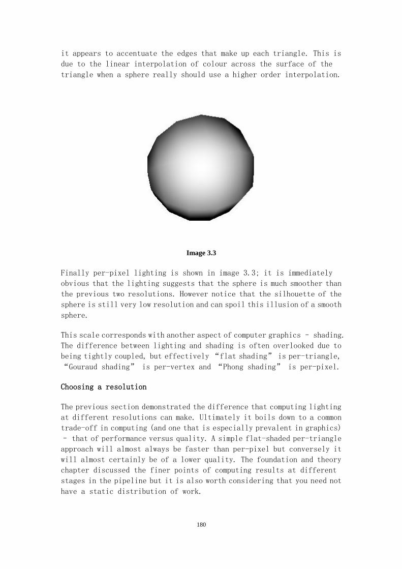
180

it appears to accentuate the edges that make up each triangle. This is

due to the linear interpolation of colour across the surface of the

triangle when a sphere really should use a higher order interpolation.

Image 3.3

Finally per-pixel lighting is shown in image 3.3; it is immediately

obvious that the lighting suggests that the sphere is much smoother than

the previous two resolutions. However notice that the silhouette of the

sphere is still very low resolution and can spoil this illusion of a smooth

sphere.

This scale corresponds with another aspect of computer graphics – shading.

The difference between lighting and shading is often overlooked due to

being tightly coupled, but effectively “flat shading” is per-triangle,

“Gouraud shading” is per-vertex and “Phong shading” is per-pixel.

Choosing a resolution

The previous section demonstrated the difference that computing lighting

at different resolutions can make. Ultimately it boils down to a common

trade-off in computing (and one that is especially prevalent in graphics)

– that of performance versus quality. A simple flat-shaded per-triangle

approach will almost always be faster than per-pixel but conversely it

will almost certainly be of a lower quality. The foundation and theory

chapter discussed the finer points of computing results at different

stages in the pipeline but it is also worth considering that you need not

have a static distribution of work.

181

More specifically it is perfectly reasonable to consider an LOD (Level

Of Detail) algorithm for lighting. Using such a system may qualify as a

regular optimization that improves overall speed but it could also allow

dynamic balancing of quality where it really matters. For example, distant

background objects may have their resolution reduced to per-triangle

whereas a foreground character may utilize a complex high resolution

per-pixel technique. As the character moves away or as the background

becomes more important the resolution of lighting calculations can change

accordingly.

Creating The Source Data

Per-pixel lighting requires the model being rendered to have a texture

map that provides the modified surface normal vectors. This input is often

referred to as a ‘Normal Map’. Whilst this is the fundamental source

of input it is possible that additional data can be required, as will be

demonstrated later in this chapter.

Normal maps can be defined in a number of different coordinate systems

– primarily object space or tangent space.

Object space, also referred to as model space, is the coordinate system

that the source geometry is defined in. Typically this will be within a

unit-volume centred at the origin and rely on the ‘world transform’ to

scale, position and orient it with regards to other objects in the scene.

Each pixel in the normal map stores a vector in object-space and the

light’s properties will need to be transformed from world space to object

space for the calculations to be performed. This makes computation very

simple by comparison to tangent-space such that object-space normal

mapping will typically be faster. Normal map and geometry are explicitly

coupled making re-use very difficult and increasing storage requirements,

but an advantage is that it allows for easy addition of decals to the

surface. Applying object-space normal maps to geometry that is animated

or deformable is difficult because as soon as the geometry upon which the

texture is mapped is altered the data stored in the normal map becomes

invalid. Updating or compensating for this at run-time can be very costly.

Tangent space is used for the remainder of this chapter and will be

explained in more detail later. Fundamentally normal vectors stored in

tangent space are tied to their texture (surface detail in any normal map

often corresponds with other textures mapped to the same pixels) rather

than the underlying geometry; consequently they will be much more

re-usable. The disadvantage is that they require more computation as well

as additional per-vertex attributes (or even more computation to runtime

182

generate these attributes). Many multimedia applications have enormous

requirements for art assets that anything to reduce the quantity to be

authored or to be stored at runtime is a definite advantage. This

perspective tends to favour tangent-space over object-space and

consequently most implementations of per-pixel lighting will use

tangent-space normal maps.

There is no required method for creating the source data and for the most

part it entirely depends on what the eventual normal map will be used for

as well as its relation to any other input data. Conceptually there are

two options - artistically or dynamically.

For the former it relies on an artist using appropriate tools to author

a normal-map in much the same way as they might generate other texture

data. Several industry standard tools offer features to assist in this

as well as there being a number of “tricks of the trade” for generating

normal map data using cameras and carefully constructed lighting

environments. This approach may well generate higher quality results but

it can quite easily create a lot of work for artists and may not be an

effective use of their time.

The alternative is to use one or more computer algorithms or techniques

to generate the normal maps. Depending on the complexity of the algorithm

this can be used to great effect and it also automates the process – which

can be a substantial benefit.

A simple but effective approach is to start with height-map data,

conventionally this is a grey-scale image where black is the lowest and

white is the highest. Then, for each pixel, you can inspect neighbouring

elements and determine the normal vector according to the gradients. The

D3DX10 library provides a convenient function to do exactly this:

D3DX10ComputeNormalMap().

A more complex approach is actually to take a high-resolution mesh and

use normal maps to encode high-frequency surface variations in the texture

and map this over low-resolution geometry. This has been used to great

effect by several commercial tools (such as ZBrush and Mudbox) and

graphics engines (such as Unreal Engine 3 and CryTek’s PolyBump

technology). This process allows the artist to create content at a high

resolution (possibly using hundreds or thousands of times more polygons)

yet have it displayed at interactive frame rates with a minimal loss of

quality. However, generating normal maps using this approach is beyond

the scope of this text.

183

Storing The Source Data

A typical normal vector is stored in terms of X, Y and Z values – each

of which are between -1 and +1 and giving the overall vector a length of

1. However, texture data is typically stored as Red, Green and Blue

intensity information. More specifically it is unusual to have negative

colour intensities – they will more typically be defined in the 0 to 1

range rather than the -1 to +1 range that a vector requires. This poses

the challenge of mapping information between the two formats.

Direct3D 10 makes this job a little easier than with Direct3D 9 simply

due to the larger number of guaranteed texture formats. In particular the

guaranteed presence of several “High Dynamic Range” formats means you

can avoid any sort of mapping and store the texture data in exactly the

same way that your application might wish to deal with (e.g. D3DXVECTOR3

maps directly to DXGI_FORMAT_R32G32B32_FLOAT). However doing such a

simple conversion has distinct storage-space considerations. A modest

96bit per pixel 512x512 normal map will require 3mb of VRAM which, on its

own, isn’t so significant but if you want per-pixel lighting on a large

number of objects then you can quite quickly see how you might exhaust

available memory (don’t be fooled by the new WDDM virtualization – if

you blow all the real VRAM it may still work but performance is likely

to suffer due to the paging overhead).

A more conventional format might be DXGI_FORMAT_R8G8B8A8_SNORM – this

requires only a third of the VRAM as the previous example. It is

immediately noticeable that we are now only using 8bits per component

instead of the full 32bit of the previous example; this might set alarm

bells ringing but experience with this technology in previous versions

of Direct3D has shown it to be relatively unimportant. You are more likely

to generate quality errors in other places.

Another useful approach to storing normal-maps is to consider a

two-component form. The DXGI format list offers a number of two-component

pixel formats such as 8, 16 and 32 bit/channel Red/Green only textures

(DXGI_FORMAT_R8G8_*, DXGI_FORMAT_R16G16_* and DXGI_FORMAT_R32G32_*).

Use of these formats requires a bit more work on the part of the programmer

and doesn’t necessarily work in every situation.

184

As shown in the above equation a unit vector can be expressed as a simple

summation equal to one. If we rearrange the above equation for the Z

component we get:

The immediate problem is that there are two, positive or negative, values

for the Z component. Given that we are using this technique to perturb

normal vectors across the surface we can, in most cases, assume that the

vector points away from the surface – more specifically, we can assume

it will be the positive value. For tangent-space normals the Z (blue

channel) is pointing away from the surface. Using the following HLSL

function we can sample a 2-component texture and then reconstruct the

original 3-component one:

float2 n = tex2D( sampler, t ).rg;

float z = sqrt( 1 – (n.r * n.r) – (n.g * n.g) );

float3 normal = normalize( float3( n.r, n.g, z ) );

This trick works well for tangent-space normal maps but tends to fall apart

when dealing with object or world space normal vectors (which are much

less common but do have valid uses). Given that it works for the majority

of cases and gives a neat 33% storage improvement it is well worth

considering.

To go even further you can consider using the block-compressed formats

(analogous to the DXT1-5 formats from previous versions of Direct3D). In

particular DXGI_FORMAT_BC5_SNORM works well with normal maps as it offers

dual independent components (meaning we have to decode a 2-component

normal to 3-component as previously discussed).

Block compressed formats work on 4x4 blocks of pixels thus it should come

as no surprise that the overall texture dimensions must be multiples of

four. If you stick with conventional 2n dimensions then this shouldn’t

matter in the slightest. When using DXGI_FORMAT_BC5_SNORM we will require

16 bytes per 4x4 block – which is at least a 2:1 compression ratio (best

case would be 12:1).

185

Diagram 3.4

DXGI_FORMAT_BC5_SNORM stores two independent colours encoded as 8 bit

Red/Green – effectively two DXGI_FORMAT_R8G8_SNORM pixels. From the two

values for each colour it is possible to generate six other intermediary

values via interpolation – for 8 shades of red and 8 shades of green.

For each of the 16 pixels in the 4x4 grid two 3 bit values are stored (3

bits can represent 8 different values) which are used to look-up one of

the 8 shades of red or green.

It is worth noting that this format is not a lossless compression system

– you will get lower quality results when using compressed formats.

Despite this it remains mostly trial-and-error as to whether this will

be noticeable in the final image.

Apart from the aforementioned need to decode from 2-component to

3-component the pixel shader needs not have any further involvement –

the GPU is responsible for decoding the compressed data (it also performs

filtering and blending at 8 bit resolution) upon request.

186

As a brief summary, the following table shows the various formats and

methods discussed thus far:

Pixel Format Storage

Per-Pixel

Storage for a

512x512

normal-map (with

full mip-chain)

Comments

R32G32B32_FLOAT 12 bytes 3.0mb (4mb) Easiest to work with, maps to

data-types used by the application

R8G8B8A8_SNORM 4 bytes 1.0mb (1.33mb)

Requires the application to re-map

input formats. One unused channel

(Alpha), could be used to store

additional data.

R11G11B10_FLOAT 4 bytes 1.0mb (1.33mb) Requires the application to re-map

input formats.

R32G32_FLOAT 8 bytes 2.0mb (2.66mb)

Application and storage data-types

match, but requires the pixel shader to

decode to 3-component form

R16G16_FLOAT 4 bytes 1.0mb (1.33mb)

Requires the application to re-map

input formats and the pixel shader

must decode to 3-component form

R8G8_SNORM 2 bytes 512kb (683kb) Same as above

BC5_SNORM 1 byte 256kb (341kb)

Texture must have dimensions that are

multiple of four, is a compressed

format so quality may suffer and will

require decoding in the pixel shader

Thinking about the storage format for your normal maps is without a doubt

a good idea – as is seen in many parts of computer graphics, there is

almost always a trade-off between quality, storage and performance. It

is worth considering the above choices in a broad context where you might

be dealing with tens, hundreds or even thousands of normal-maps in a given

scene; by reducing the storage space required you can either increase the

resolution (a 2048x2048 compressed normal map is only 1mb larger than an

uncompressed 512x512 map) or simply increase the number of normal maps

(For one 512x512 uncompressed normal maps you could store 12 compressed

maps).

On a related, but slightly different note it is worth considering the use

of mip-mapping with normal maps. In particular it can be a very easy way

of introducing visual errors into your final image.

187

Without mip-maps it is possible to introduce aliasing that causes the

final image to sparkle – very small movements of the geometry can result

in substantially different parts of the normal-map being sampled if it

is of a very high resolution. This can mean that the inputs into the

lighting equation dramatically change and thus you get a noticeable visual

artefact.

Using mip-maps helps to eliminate this problem but it can allow for

different errors to creep in. Unless you create your normal maps with a

tool that is specifically aware of what the content really is then you

may find regular image-processing techniques actually break the stored

data. In particular, D3DX can generate mip-chains for you when you load

your image but when it down-samples and blends neighbouring pixels the

result may no longer be decoded as a unit-length vector. If you then feed

these un-normalised vectors into lighting equations you’ll often get

dull and flat results. This may not always be noticeable (by definition,

lower mip-maps are used when the contribution to the final image is

relatively small) but it is worth bearing in mind. A simple remedy is to

ensure that your normalize() any vectors sampled from a texture, but this

will add to the arithmetic complexity of the shader.

There is one final storage-reduction trick that can beat all of the methods

discussed previously in this section: Run-time normal generation. A

normal map is often generated from a height-map but as will be shown later

in this chapter the height map might also be an input into a per-pixel

lighting algorithm.

This effectively duplicates the data – the height map is being uploaded

to the GPU and additional data derived from this is also being uploaded.

Therefore an obvious optimization is to upload only the original data and

then derive the normal map as and when required.

The trade-off is the performance decrease due to the extra work done versus

the reduction in storage. In some applications storage space can be much

more valuable than performance therefore making this a compelling option.

// Determine the offsets

float2 o1 = float2( vPixelSize.x, 0.0f );

float2 o2 = float2( 0.0f, vPixelSize.y );

// Take three samples to determine two vectors that can be

// use to generate the normal at this pixel

float h0 = texHeightMap.Sample( DefaultSampler, tc ).r;

float h1 = texHeightMap.Sample( DefaultSampler, tc + o1 ).r;

float h2 = texHeightMap.Sample( DefaultSampler, tc + o2 ).r;

188

float3 v01 = float3( o1, h1 - h0 );

float3 v02 = float3( o2, h2 - h0 );

float3 n = cross( v01, v02 );

// Can be useful to scale the Z component to tweak the

// amount bumps show up, less than 1.0 will make them

// more apparent, greater than 1.0 will smooth them out

n.z *= 0.5f;

return normalize( n );

The previous code listing shows a simple way of generating a normal from

a height-map. It uses the standard method for generating a triangle’s

face normal. The quality, shown in image 3.5, proves to be much lower than

that generated by an offline pre-processor. An alternative is to make use

of Sobel filter kernels to determine the U and V gradients; this requires

eight samples but has much lower arithmetic overheads and has generates

better quality result.

The following two kernels are used to generate the U and V gradients:

Normal vectors have a length of 1.0 which combined with the U and V

gradient’s allows the computation of the missing 3rd element of the

normal:

189

This can all be put together in HLSL:

// Compute the necessary offsets:

float2 o00 = tc + float2( -vPixelSize.x, -vPixelSize.y );

float2 o10 = tc + float2( 0.0f, -vPixelSize.y );

float2 o20 = tc + float2( vPixelSize.x, -vPixelSize.y );

float2 o01 = tc + float2( -vPixelSize.x, 0.0f );

float2 o21 = tc + float2( vPixelSize.x, 0.0f );

float2 o02 = tc + float2( -vPixelSize.x, vPixelSize.y );

float2 o12 = tc + float2( 0.0f, vPixelSize.y );

float2 o22 = tc + float2( vPixelSize.x, vPixelSize.y );

// Use of the sobel filter requires the eight samples

// surrounding the current pixel:

float h00 = texHeightMap.Sample( DefaultSampler, o00 ).r;








// Evaluate the Sobel filters

float Gx = h00 - h20 + 2.0f * h01 - 2.0f * h21 + h02 - h22;

float Gy = h00 + 2.0f * h10 + h20 - h02 - 2.0f * h12 - h22;

// Generate the missing Z

float Gz = 0.5f * sqrt( 1.0f - Gx * Gx - Gy * Gy );

// Make sure the returned normal is of unit length

return normalize( float3( 2.0f * Gx, 2.0f * Gy, Gz ) );

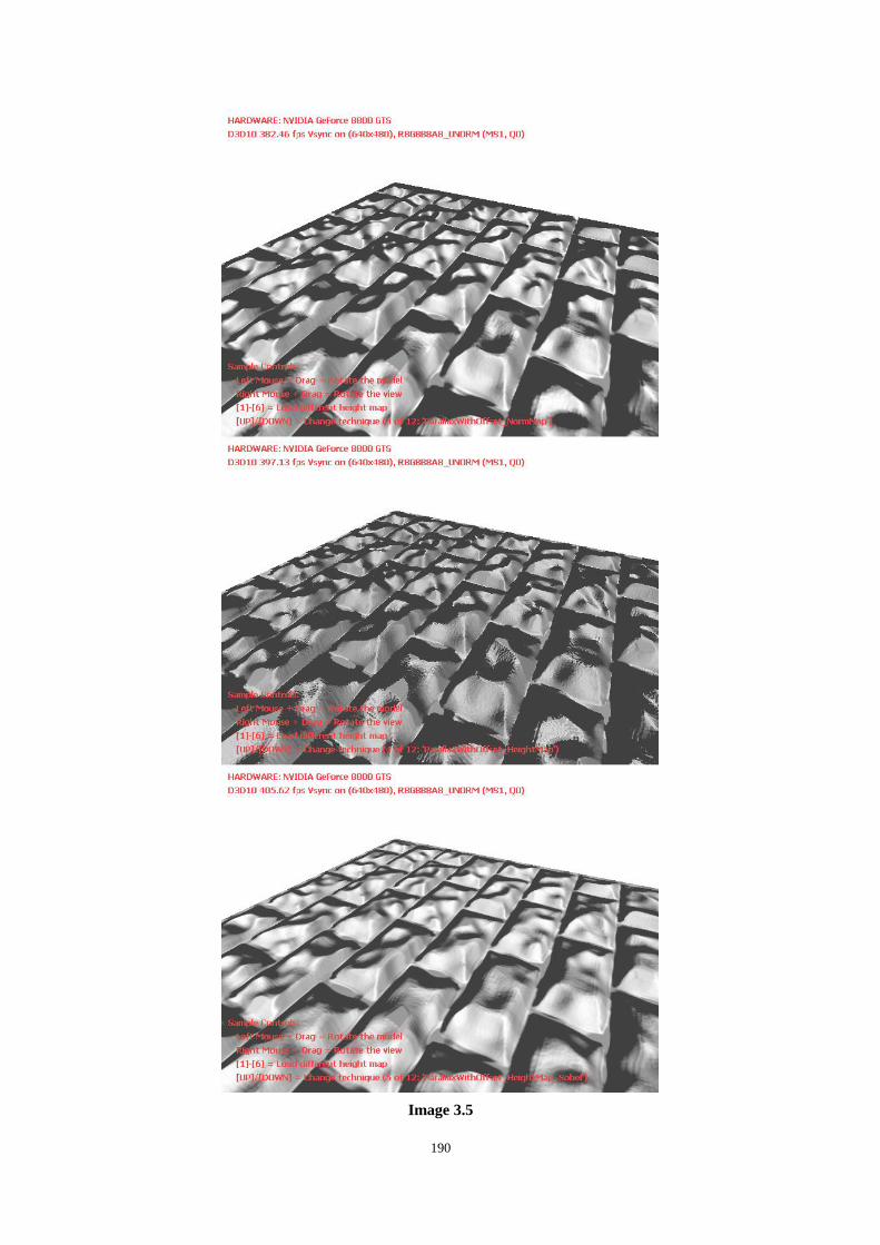
190

Image 3.5

191

Reading from a texture, top, computing using three samples, middle, and

the Sobel filter, bottom, all generate different quality results. In

general a pre-computed normal map will be of a higher quality but it can

require a substantial amount of storage space. The Sobel filter is

probably the best trade-off for performance versus storage.

This can all be put together to form the following HLSL function:

float3 FetchNormalVector

(

float2 tc,

uniform bool readFromTexture,

uniform bool useSobelFilter

)

{

if( readFromTexture )

{

// Use the simple pre-computed look-up

float3 n = texNormalMap.Sample( DefaultSampler,

tc ).rgb;

return normalize( n * 2.0f - 1.0f );

}

else

{

if( useSobelFilter )

{

// Previously discussed code for Sobel filter

// goes here.

}

else

{

// Previously discussed code for 3-sample

// evaluation goes here.

}

}

}

This function is relied upon for the techniques demonstrated later in the

chapter. It encapsulates the three main methods for fetching per-pixel

normal vectors and allows for easy experimentation. There are two very

important points to note with the above code. Both of which will result

in an incorrect image and can be really quite difficult bugs to track down.

Firstly, the underlying normal-map texture is stored in

DXGI_FORMAT_R8G8B8_UNORM – that is, each component is in the range 0.0

192

to 1.0 whereas the vector we want should be in the -1.0 to +1.0 range.

A simple multiply by two and subtract one will perform the correct

remapping, but it is all too easy to forget!

Storing normal maps in _UNORM form is fairly standard, but as previously

discussed not compulsory. This initial remapping may not be required

depending on the chosen implementation.

Secondly, the Sample() call is explicitly swizzled to ‘rgb’ before being

manipulated by the previous remapping and most importantly before being

an input into the normalize() intrinsic. The return value from Sample()

is a float4 which would result in a 4D vector normalization that would

then be truncated to the float3 declaration used to hold the results.

Because the incoming texture contains only three components it will be

padded to a 4D vector with a 1.0 value for the 4th component. This throws

the normalize() result out and the 3D vector we pass into the lighting

calculations is no longer unit-length. The net result is that lighting

can appear to be dull due to the way that the Lambertian N•L scalar can

never be greater than this shortened and corrupted input vector. By

forcing the sample to be a 3D vector before normalization we can completely

avoid this problem.

Moving From Per-Vertex To Per-Pixel

For this section of the book we will be using tangent-space normal maps

(as opposed to the previously mentioned object-space normal maps). This

gets slightly tricky in that the per-vertex attributes that our geometry

is defined with are no longer in the same coordinate system as the vectors

stored in the normal map texture. Thus it becomes necessary to transform

all inputs into the same coordinate frame – failure to do this will

generate noticeably incorrect results.

As with most transformations we can go in either direction – we could

transform the normal-map into world space coordinates or we could

transform per-vertex attributes to tangent-space coordinates. It is

common to do the latter simply because it requires less computation (which

equates to better performance). However there are still a number of

situations where the choice isn’t so obvious or you may want to implement

it differently. For example, environment mapping needs a world-space

normal and using a vertex shader to transform light vectors to tangent

space can chew up a large number of interpolators (the resource used to

transport data between shader units) if many lights are being used.

193

The most important point is that we perform any calculations on inputs

that are all in the same coordinate system. Failure to do this (e.g.

performing the dot-product on a world-space and tangent-space vector)

results in very noticeable errors which, from the source code, can be quite

tricky to spot.

From a mathematical point of view a 3D coordinate system is defined through

three linearly independent basis vectors. For tangent space we will be

using tangent, normal and bitangent (this is often incorrectly referred

to as “binormal”) vectors which are based on the texture coordinates

that map the normal map over the surface of the triangle.

Diagram 3.6

The preceding diagram shows how this coordinate system looks; it is worth

noting that the tangent frame is defined for the individual triangle.

Whilst Direct3D 10, via the SV_PrimitiveID system-generated value, would

allow us to store per-primitive attributes it is easier (and more common)

to attach the vectors as per-vertex attributes.

Diagram 3.7

194

Providing the vectors as per-vertex attributes introduces one potential

problem though – the case where two triangles share the same vertex yet

have different coordinate frames. Diagram 3.7 shows an example of a

situation known as a “bow tie”. The vertex linking the two triangles

might have a common texture coordinate, but the other two vertices in each

triangle result in a different per-triangle coordinate frame. Solving

this problem isn’t difficult but it does require the

splitting/duplication of vertex data which can lead to less efficient

vertex processing (less utilization of the post-transform vertex cache

for example) and increased storage requirements.

Generating the tangent frame is relatively simple and depending on the

available art tools may not even be required in the main application. It

is important to note that the tangent frame is actually a per-triangle

attribute and it is quite common to store averages of neighbouring

triangles for the per-vertex attributes.

Let V0, V1 and V2 be the vertex positions making up the triangle

Define A and B as:

Let TC0, TC1 and TC2 be the texture coordinates at each of the vertices

Define P and Q as:

We can now express the Tangent and Bitangent with the following equation:

The preceding equation gives us unnormalized vectors, so the next step is to normalize:

195

As well as the Tangent and Bitangent we also need the normal, N:

The three vectors might not be exactly orthogonal but we can use the Gram-Schmidt

algorithm to orthogonalize:

These vectors can then be rearranged for the following, final, matrix:

For more in-depth information on the above method, refer to [Lengyel03].

Implementing the algorithm is not difficult, but D3DX9 had a function to

do all this work for you. At the time of writing this function is not in

D3DX10, but there are ways of using the more advanced D3DX9 mesh library

as a pre-processor for D3DX10 meshes until the D3DX10 library matures.

The sample code accompanying this section demonstrates a way of achieving

this.

In much the same way that we could choose the storage format for the

normal-map texture we also have a lot of choice about how the tangent-space

coordinate frame is attached to each vertex. This can have notable

performance (especially if using animated or deformable models) and

storage trade-offs as will be demonstrated in the following sections:

196

Uncompressed storage'

This method is very simple – the application can compute the necessary

basis vectors or get the D3DX library to do the work and then simply attach

the raw data to each vertex. This is both easy to understand and

straight-forward to write code for. The problem is, quite simply, that

it is uncompressed and that it stands to inflate our storage requirements.

More subtly it can also affect the performance of our rendering.

In particular the GPU will usually be required to stream vertex data from

the main video memory into the local cache before the vertex shader can

operate on the information. It is a simple case that the more data the

chip has to stream the slower the overall performance is likely to be.

Given that a simple vertex might be a position, normal and texture

coordinate (32 bytes) adding an additional 36 bytes (112.5%) seems a

little heavy.

For uncompressed mode it would be necessary to use the following

declaration:

D3D10_INPUT_ELEMENT_DESC uncompressed[] =

{

{

"POSITION", 0,

DXGI_FORMAT_R32G32B32_FLOAT, 0, 0,

D3D10_INPUT_PER_VERTEX_DATA, 0

},

{

"NORMAL", 0,



},

{

"BITANGENT", 0,



},

{

"TANGENT", 0,



},

{

"TEXCOORD", 0,

DXGI_FORMAT_R32G32_FLOAT, 0, 48,

197


},

};

This would correspond to the following input into a vertex shader:

struct vsUncompressed

{

float3 position : POSITION;

float3 normal : NORMAL;

float3 bitangent : BITANGENT;

float3 tangent : TANGENT;

float2 texcoord : TEXCOORD;

};

Compress to 2-axis

The next step on from uncompressed data is to trade the storage of one

vector against additional computation costs. Using the cross-product

equation we can reconstruct the bitangent vector provided we know both

of the tangent and normal vectors. This is a relatively easy storage space

win – the reduction of 12 bytes per vertex, down to adding only 24 bytes,

is almost always going to be more beneficial than any overhead introduced

by the cross product operation.

There is one complication in using this technique: tangent-space

handedness. When trying to reconstruct the missing vector there are two

possible, opposite, directions similar to the situation encountered when

storing normal vectors in a 2-channel texture. The resolution to this

issue is to multiply the cross product of the normal and tangent vectors

by a ±1 bias. This value is simply the determinant of the matrix produced

in step-9 of the preceding instructions on computing the tangent-space

transformation matrix.

The application configuration would look like:

D3D10_INPUT_ELEMENT_DESC uncompressed2Axis[] =

{

{

"POSITION", 0,



},

{

"TANGENT", 0,

198



},

{

"NORMAL", 0,



},

{

"BIAS", 0,

DXGI_FORMAT_R32_FLOAT, 0, 36,


},

{

"TEXCOORD", 0,



},

};

This corresponds to the following input into the vertex shader:

struct vsUncompressed2Axis

{

float3 position : POSITION;

float3 tangent : TANGENT;

float3 normal : NORMAL;

float bias : BIAS


};

For clarity the bias is separated into a separate attribute but in practice

it would be valid to widen either the tangent or normal attributes to a

4-component form and store the bias in the 4th component. If doing this

be careful to use the appropriate ‘xyz’ swizzle when decoding the

missing vector.

The vectors can then be decoded using this simple HLSL fragment:

float3 bitangent = cross( vertex.tangent, vertex.tangent );

bitangent *= vertex.bias;

bitangent = normalize( bitangent );

Compress to half-precision

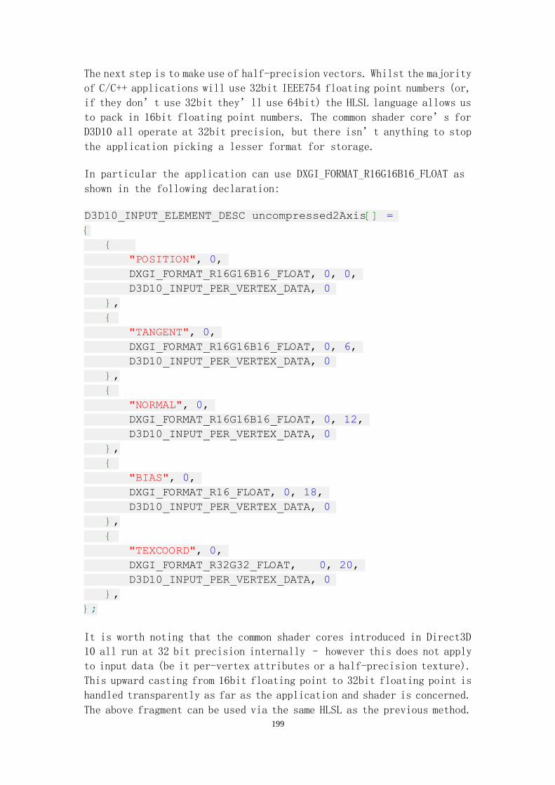
199

The next step is to make use of half-precision vectors. Whilst the majority

of C/C++ applications will use 32bit IEEE754 floating point numbers (or,

if they don’t use 32bit they’ll use 64bit) the HLSL language allows us

to pack in 16bit floating point numbers. The common shader core’s for

D3D10 all operate at 32bit precision, but there isn’t anything to stop

the application picking a lesser format for storage.

In particular the application can use DXGI_FORMAT_R16G16B16_FLOAT as

shown in the following declaration:

D3D10_INPUT_ELEMENT_DESC uncompressed2Axis[] =

{

{

"POSITION", 0,



},

{

"TANGENT", 0,



},

{

"NORMAL", 0,



},

{

"BIAS", 0,

DXGI_FORMAT_R16_FLOAT, 0, 18,


},

{

"TEXCOORD", 0,



},

};

It is worth noting that the common shader cores introduced in Direct3D

10 all run at 32 bit precision internally – however this does not apply

to input data (be it per-vertex attributes or a half-precision texture).

This upward casting from 16bit floating point to 32bit floating point is

handled transparently as far as the application and shader is concerned.

The above fragment can be used via the same HLSL as the previous method.

200

Compress to 8-bit integer

The next step would be to consider properly compressing the per-vertex

attributes. Using half-precision vectors is a form of compression, but

more of a convenient one as opposed to an explicit attempt at compression.

Using D3D10’s new integer instruction set could yield numerous packing

opportunities and based on trial-and-error it is possible to greatly

reduce the amount of per-vertex data. As with most compression schemes

the result is a trade-off between storage requirements versus quality.

A key observation, based in part on the discussion of encoding normal

vectors in textures, is that it is possible to store each component of

a vector in an 8 bit integer quantity. Experience shows that this doesn’t

usually result in a substantial loss of quality therefore making it a

viable choice in this situation. The more adventurous programmer could

look into using Direct3D 10’s new integer instruction set to implement

fixed-point storage with the DXGI_FORMAT_R10G10B10A2 formats. This could

be a useful middle-ground between using 8bit integers and half-precision

floating point quantity. The 2-bit alpha channel may seem useless, but

it is a good candidate for storing the bias component discussed in the

previous section.

The new DXGI formats for D3D10 don’t actually have a 3-channel 8 bit

format, only 1, 2 and 4 channel forms. Consequently the following

structure is slightly unintuitive as it splits the individual vectors up

so as not to waste an additional byte per attribute:

D3D10_INPUT_ELEMENT_DESC compressed8Bit2Axis[] =

{

{

"POSITION", 0,



},

{

"TANGENT_X", 0,

DXGI_FORMAT_R8_SNORM, 0, 12,


},

{

"TANGENT_Y", 0,



},

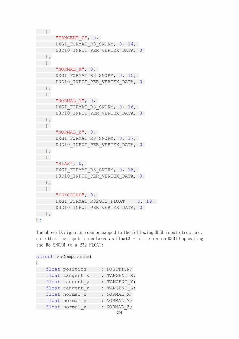
201

{

"TANGENT_Z", 0,



},

{

"NORMAL_X", 0,



},

{

"NORMAL_Y", 0,



},

{

"NORMAL_Z", 0,



},

{

"BIAS", 0,



},

{

"TEXCOORD", 0,



},

};

The above IA signature can be mapped to the following HLSL input structure,

note that the input is declared as float3 – it relies on D3D10 upscaling

the R8_SNORM to a R32_FLOAT:

struct vsCompressed

{

float position : POSITION;

float tangent_x : TANGENT_X;

float tangent_y : TANGENT_Y;

float tangent_z : TANGENT_Z;

float normal_x : NORMAL_X;

float normal_y : NORMAL_Y;

float normal_z : NORMAL_Z;

202

float bias : BIAS;


};

Compute with the geometry shader

As previously discussed in this section, the tangent-frame information

is really a per-triangle attribute rather than per-vertex. Attaching the

information to the vertices is more of a legacy method – these techniques

all work under Direct3D 9 where there was no scope for either generating

or attaching per-primitive attributes.

Simply put we can use the new Geometry Shader stage to generate the

tangent-space vectors dynamically on the GPU. This reduces the storage

requirements (remember that for a given triangle we could have three sets

of tangent-space vectors if implemented per-vertex) and associated memory

bandwidth requirements. It also eliminates the case of “bow ties” where

conflicting data requires a shared vertex to be duplicated and split.

The obvious downside is that it trades storage requirements against

execution time requirements; the geometry shader will have to compute the

vectors every time the triangle is rendered – regardless of whether it

has actually changed. For static geometry it is most likely a better option

to compute the results on the CPU and upload it; dynamic and procedural

geometry might well see a substantial performance improvement by

computing entirely on the GPU. Using previous techniques any change to

the geometry would most likely require the CPU to intervene and both

recalculate and re-upload the results – neither of which is good for

performance.

The following HLSL function can be used in a Geometry Shader to generate

the appropriate transform matrix:

float3x3 ComputeTangentSpaceMatrix

(

in float3 pos[3],

in float2 tc[3]

)

{

float3 A = pos[1] - pos[0];

float3 B = pos[2] - pos[0];

float2 P = tc[1] - tc[0];

float2 Q = tc[2] - tc[0];

203

float fraction = 1.0f / ( P.x * Q.y - Q.x * P.y );

float3 normal = normalize( cross( A, B ) );

float3 tangent = float3

(

(Q.y * A.x - P.y * B.x) * fraction,

(Q.y * A.y - P.y * B.y) * fraction,

(Q.y * A.z - P.y * B.z) * fraction

);

float3 bitangent = float3

(

(P.x * B.x - Q.x * A.x) * fraction,

(P.x * B.y - Q.x * A.y) * fraction,

(P.x * B.z - Q.x * A.z) * fraction

);

// Some simple aliases

float NdotT = dot( normal, tangent );

float NdotB = dot( normal, bitangent );

float TdotB = dot( tangent, bitangent );

// Apply Gram-Schmidt orthogonalization

tangent = tangent - NdotT * normal;

bitangent = bitangent - NdotB * normal - TdotB * tangent;

// Pack the vectors into the matrix output

float3x3 tsMatrix;

tsMatrix[0] = tangent;

tsMatrix[1] = bitangent;

tsMatrix[2] = normal;

return tsMatrix;

}

CPU based computation will typically include adjacent triangles when

computing per-vertex attributes – a simple case of averaging the vectors

for each face that shares a particular vertex. This may be mathematically

incorrect but it can allow for a more aesthetically pleasing result in

much the same way that averaging vertex normal vectors can give the

impression that the surface is smoother than it really is (refer back to

image 3.2). By computing the tangent-space transform in the geometry

204

shader this is still possible if adjacency information is used, but it

would mean calling the ComputeTangentSpaceMatrix() function four times

per-primitive.

Summary:

Method Additional

Storage Comments

Uncompressed 36 bytes/vertex Easiest to work with, but may well inflate storage and

bandwidth requirements

2-axis and compute 3rd

in the shader 28 bytes/vertex

Relatively easy to work with, but offloads storage

against a minimal run-time computation cost

Half-Precision vectors 14 bytes/vertex Slightly more complex to work with and trades

storage space against computation cost

Compressed vectors 7 bytes/vertex Potential loss of quality due to low-resolution of the

data

Geometry Shader None! computation cost in favour of not having any

additional data storage

A Framework For Per-Pixel Lighting

Before covering the actual algorithms for per-pixel lighting it is useful

to define a common framework. From a high-level the following three

algorithms do only two things:

1. Compute the texture coordinate

2. Compute the illumination

The remainder of this chapter deals with the first part and the next six

deal with the second part. This chapter uses a very simple Lambertian N•L

computation for illumination as a form of place-holder for the models

discussed in later chapters.

Each of the techniques can use the same vertex shader to perform the

tangent-space transformations:

VS_TS_OUTPUT vsTangentSpace( in VS_INPUT v )

{

VS_TS_OUTPUT o = (VS_TS_OUTPUT)0;

// Transform the incoming model-space position to

// projection space - a standard VS operation.

205

o.position = mul( float4( v.position, 1.0f ),

mWorldViewProj );

// The world-space vertex position is useful for

// later calculations.

float3 pWorld = mul( float4( v.position, 1.0f ),

mWorld ).xyz;

// The per-vertex attributes are in model space, so we

// need to transform them to world space before we can

// generate a world->tangent transformation

float3 vTangentWS = mul( v.tangent,

(float3x3)mWorld );

float3 vBitangentWS = mul( v.bitangent,

(float3x3)mWorld );

float3 vNormalWS = mul( v.normal,

(float3x3)mWorld );

// Pack the data into the matrix for transforming

// the actual input data

float3x3 mWorldToTangentSpace;

mWorldToTangentSpace[0] = normalize( vTangentWS );

mWorldToTangentSpace[1] = normalize( vBitangentWS );

mWorldToTangentSpace[2] = normalize( vNormalWS );

// Use the matrix to transform all necessary

// inputs for the pixel shader.

o.lightdir = mul( mWorldToTangentSpace, -vLightDir );

o.viewdir = pCameraPosition - pWorld;

o.viewdir = mul( mWorldToTangentSpace, o.viewdir );

// Pass through any other necessary attributes

o.texcoord = v.texcoord;

return o;

}

The code included above only transforms two vectors into tangent space

– the light and view directions. These are standard inputs into most BRDF

lighting models and all that is required for the techniques discussed

later in this section, but there more complex techniques may well need

to transform additional inputs – simply add the additional code towards

the end of the above vertex shader.

206

The vertex shader sets up the inputs for the pixel shader which is where

the two main pieces of work are performed:

float4 psMain( in VS_TS_OUTPUT_V ) : SV_TARGET

{

// Normalize the input vectors

float3 view = normalize( v.viewdir );

float3 light = normalize( v.lightdir );

// Determine the offset for this pixel

float2 offset = ComputeOffset( v.texcoord, view );

// Retrieve the normal

float3 normal = FetchNormalVector( v.texcoord, true );

// Evaluate the lighting model

float4 colour = ComputeIllumination( normal, view,

light );

// Return the final colour

return colour;

}

The ComputeOffset() and ComputeIllumination() calls are abstractions for

the main pieces of work. The former is discussed for the remainder of this

section and the latter represents the BRDF lighting model that is

discussed over the next six chapters.

In developing more complex material systems (for which the lighting models

are simply a foundation) the framework proposed here would need to be

changed. As should be immediately obvious, the input vertex data is

assumed to be using uncompressed tangent-space vectors; it is also worth

noting that this framework is suitable only for a single light source.

Real-world applications are more likely to use a loop (using a for()

construct) to handle multiple lights. For simplicity these are not

included here but they are all valid modifications that can be implemented

on top of this simple example.

Simple Normal Mapping

This technique is the closest to James Blinn’s original 1978 paper and

is also the simplest of the three being covered in this chapter. Despite

its simplicity it is a very effective technique that can be used to great

effect.

207

The code-listing presented as part of the previous section is in fact

simple normal mapping. As described, these three techniques deal with

perturbing the normal across the surface in order to simulate a more

detailed surface. For simple normal mapping with just read a new normal

directly from the normal map texture bound to this particular primitive.

The pixel shader does not need to do any additional work – the vertex

shader has already transformed the input data into tangent space (which

is the same coordinate system that the normal map is stored in) and the

texture coordinate does not need to be modified. Therefore the complete

pixel shader is as follows:

float4 psNormalMap( in VS_TS_OUTPUT v ) : SV_TARGET

{

float3 normal = FetchNormalVector( v.texcoord, true );

return ComputeIllumination( v.lightdir, normal,

0.0f );

}

The previous fragment relies on two functions one of which is included

below for reference. To simplify the source code provided to accompany

this chapter several common operations are refactored into their own

functions.

float4 ComputeIllumination

(

float3 LightDir,

float3 Normal,

float Shadow

)

{

float NdotL = dot( LightDir, Normal );

Shadow = 1.0f - Shadow;

float c = max( 0.25f, NdotL * Shadow );

return float4( c, c, c, 1.0f );

}

Refer back to the earlier discussion on run-time generation of normal

vectors from the height-map for a full explanation of the

FetchNormalVector() function.

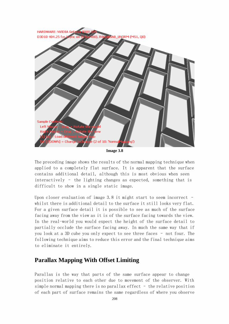
208

Image 3.8

The preceding image shows the results of the normal mapping technique when

applied to a completely flat surface. It is apparent that the surface

contains additional detail, although this is most obvious when seen

interactively – the lighting changes as expected, something that is

difficult to show in a single static image.

Upon closer evaluation of image 3.8 it might start to seem incorrect –

whilst there is additional detail to the surface it still looks very flat.

For a given surface detail it is possible to see as much of the surface

facing away from the view as it is of the surface facing towards the view.

In the real-world you would expect the height of the surface detail to

partially occlude the surface facing away. In much the same way that if

you look at a 3D cube you only expect to see three faces – not four. The

following technique aims to reduce this error and the final technique aims

to eliminate it entirely.

Parallax Mapping With Offset Limiting

Parallax is the way that parts of the same surface appear to change

position relative to each other due to movement of the observer. With

simple normal mapping there is no parallax effect – the relative position

of each part of surface remains the same regardless of where you observe

209

the surface from. It is best observed interactively when you can change

the viewing position – if the surface was actually bumpy then you’d

expect to see more/less of opposing sides of the bumps depending on where

you positioned the camera.

The next progression for per-pixel mapping requires the use of an

additional piece of per-pixel information – elevation. This is usually

easy enough to provide given that the normal map is typically generated

from a height-map (see “Creating the source data” for more discussion

on this). Simple normal mapping did not perturb the texture coordinate

before sampling the normal map, but by modifying this such that it

compensates for parallax it is possible to reduce one of the main graphical

flaws in simple normal mapping. This approach was proposed in “Parallax

Mapping with Offset Limiting: A Per-Pixel Approximation of Uneven

Surfaces” [Welsh04]. As will be shown, a relatively simple modification

to simple normal mapping can generate a substantial quality improvement.

Diagram 3.9

Diagram 3.9 shows the actual surface as the bold, black line and adds the

elevation information as the dashed line. In tracing a line from the viewer

to the pixel there are cases where it will pick the normal vector

incorrectly. Simple normal mapping provides no occlusion and makes it

possible to see parts of the surface that are facing away from the camera.

Parallax mapping with offset limiting compensates for this by inspecting

the elevation information (stored in a height-map) and offsetting the

texture coordinate so that a more accurate sample is used.

210

Diagram 3.10

By sampling the height-map at the coordinate passed down from the vertex

shader (Toriginal) we can compute an offset that we add in order to sample

the correct location (Tcorrected) for any other resources (in this

instance we only sample a normal map but sampling a diffuse texture is

also fairly standard). As shown in diagram 3.10 the offset computed by

using just the height is not actually correct and is thus only an

approximation to the proper result (Tactual). Acquiring the correct

offset is possible but is a substantially more expensive algorithm thus

making this approximation worth using.

Parallax mapping with offset limiting first has to scale the height

information which in most cases will be stored in the range 0.0 to 1.0.

Given that texture coordinates are typically constrained to a 0.0 to 1.0

range thus offsetting these by a height in the same range would be far

too much – providing wrapping/mirroring is enabled you’d almost

certainly end up fetching data that is a long way from the desired location.

As can be seen with a little experimentation, tweaking the offset

calculations for this technique can destabilise the results – at a

certain point the approximation is sufficiently wrong as to generate

noticeable artefacts in the final image.

The first step in this algorithm is to perform a simple linear

transformation on the height retrieved from the height-map:

Typical values for scale will be less than 0.05 with the bias typically

being the scale multiplied by -0.5. The actual values are partly dependent

on source data and the desired outcome. This transformed height value can

then be used to scale the offset in the direction of the viewer (a vectors

transformed to tangent space by the vertex shader). This direction will

be in the (X, Y) part of the 3D vector with the Z component representing

the steepness of the view angle at a given point.

211

The original parallax mapping approach ([Kaneko01]) divided the offset

by the view vector’s Z component which is mathematically more accurate.

However, in doing so the offset ends up becoming extremely large at grazing

angles (where the Z component approaches zero) due to the division by a

very small value. As was previously mentioned, having a large offset

results in the sampling of incorrect source data and thus you get very

noticeable graphical artefacts. The preceding equation does not divide

by the Z component thus limiting the offset to a maximum of Heightsb; it

isn’t the only way that the offset could be limited but it has the distinct

advantage that it simplifies the pixel shader rather than adds potentially

complicated methods for limiting the computed offset.

float4 psParallaxMapping

(

in VS_TS_OUTPUT v,

uniform float HEIGHT_SCALE

)

: SV_TARGET

{

// Compute the height at this location

float height = texHeightMap.Sample( DefaultSamp,

v.texcoord ).r;

height = HEIGHT_SCALE * height - (HEIGHT_SCALE / 2.0f);

// Compute the offset

float2 offsetDir = normalize( v.viewdir ).xy;

float2 offsetSample = v.texcoord + offsetDir * height;

// Take the samples with the shifted offset

float3 normal = FetchNormalVector( offsetSample, true );

// Compute the final colour

return ComputeIllumination( v.lightdir, normal, 0.0f );

}

The above code listing contains the simple modifications to the standard

framework introduced previously. Note that the only real change is

modifying the texture coordinate passed down from the vertex shader –

the remainder of the pixel shader is identical to that used in simple

normal mapping.

212

Image 3.11

The preceding image, 3.11, shows parallax mapping with a scale of 0.05

and bias of -0.025. It should be immediately obvious that the surface is

more realistic than with simple normal mapping; note how the amount of

each bump’s sloped sides varies across the surface of the geometry. This

is much closer to what the eye and brain are expecting and is thus much

more acceptable than simple normal mapping. The following image, 3.12

shows a debug output of the parallax effect – one where the value is just

the length of the computed offset. Darker areas of the surface correspond

with areas where little or no offset is required and lighter areas where

the offset is greater. Notice that the areas subject to the largest offsets

are at the glancing angles and where the surface height is greatest; the

darker area on the surface corresponds to where the view direction is close

to being perpendicular to the underlying geometry.

213

Image 3.12

Ray-Traced

This is the 3rd and final approach to per-pixel lighting that will be

covered. The previous section implemented a way to approximate the correct

offset that generates very good results given the simplicity of the change.

This section presents a hybrid technique of relief mapping ([Policarpo05]

and ‘Parallax Occlusion Mapping’ – [Tartarchuk06]). Both use much the

same theory of ray-tracing in the pixel shader to accurately compute the

correct offset and thus attain the best image quality. This is interesting

not only because of the high-quality results but also because of the way

it blurs the line between ray-traced graphics and traditional polygonal

raster graphics; two techniques that, for the most part, are considered

to be mutually exclusive.

Up-front the mention of ray-tracing might worry the more experienced

graphics programmer – arguably the primary motivation behind real-time

graphics using polygonal methods is that their performance is an order

of magnitude better than that of ray-traced equivalents. Thus ray-tracing

is synonymous with non-real-time performance. Unsurprisingly this makes

it the slowest of the three techniques demonstrated in this chapter but

this doesn’t invalidate its viability as a real-time rendering effect.

With regards to performance, previous implementations have shown best

214

performance with the more advanced shading models – version 3.0 pixel

shaders for example. The process of ray-tracing in a pixel shader benefits

greatly from a shader model that can handle dynamic looping and branching

– features that come as standard in shader model 4.0. Arguably the fact

that the software shader model is good at expressing these programming

constructs does not guarantee that the hardware is good at executing them

– but such things are beyond the scope of this text.

The previous technique introduced the use of the view-direction and relief

mapping takes this further by not just using it for a single-step offset

but to define a line from which to take multiple samples from. It is the

viewing vector that forms the ray in which we are to trace. Take the

following diagram where the bold line is the surface and the dashed line

is the one we wish to approximate (note that, unlike previous techniques,

we are using a subtractive approach – more on this later). Conventional

ray-tracing is heavy on the mathematics and fundamentally relies on

equations that test the intersection between the current ray and basic

primitives (such as planes or spheres), the ray-tracing that can be

employed for this technique simply checks whether we are above or below

the height of the surface being represented. It therefore becomes a simple

test whereby the transition from above to below the height of the surface

marks the point of intersection. Take the following diagram where the

intersection exists between the 3rd and 4th sample:

Diagram 3.13

215

Referring to any good computer graphics or even general computer science

text-book would suggest that a binary search is a perfect candidate in

this situation. Given that we would like to reduce the number of samples

taken (each of which increases the required bandwidth) a smart algorithm

such as binary search would be great. However, consider the following

diagram:

Diagram 3.14

Diagram 3.14 shows a case where the first mid-point is already beyond the

actual point of intersection. The binary search continues scanning

forward, looking for a point below the surface which it quickly finds and

then assumes the true point of intersection lies between these two – even

though the first point is incorrect.

The preceding diagram shows a relatively rare case that is usually

reserved for surfaces with high-frequency height-map information however

it hides a more subtle artefact; the relative viewer orientation need not

move a huge amount for the above characteristic to either appear or

disappear. This is one of the worst situations for computer graphics

quality – the artefact appears to flicker between visible and invisible

much like “Z-Fighting” artefacts. Luckily there is a convenient

work-around to this initial setback – a hybrid of both binary and linear

searching works quite well. The basic idea is to run a linear search to

get an initial reference point and then to improve the accuracy of this

by using a secondary binary search:

216

Diagram 3.15

The first four samples are the linear search – performed until the first

sample below the surface is found. A binary search, the 5th and 6th samples,

can then operate between the last two linear search locations which should

be above/before and below/after the true point of intersection. It is

still possible to find test-cases that fool this system, but the in the

vast majority of cases this hybrid approach is accurate.

This hybrid approach is used in the implementation of Relief Mapping and

whilst it can yield very accurate results with minimal samples it has one

problem when mapped to real hardware. The samples taken during the final

binary searching phase are classed as “dependent reads” – the location

being sampled is dependent on some arithmetic performed by the shader.

This makes it much harder for the GPU and its driver to schedule

instructions efficiently and ultimately leads to poor performance. The

linear searching phase of the algorithm does not suffer from this problem

– whilst the number of samples are dynamic the actual locations are at

well defined intervals and not dependent on any arithmetic in the shader.

The Parallax Occlusion Mapping technique utilizes only a linear search

in an attempt to make the algorithm as optimal as possible for current

GPU architectures. The final refinement stage can be implemented in

arithmetic rather than as an additional search which yields equivalent

results and is therefore a perfectly valid optimization.

This final refinement stage requires solving for the intersection of the

surface and the ray corresponding to the view direction. Due to linear

filtering we can assume that the pixels sampled for the height of the

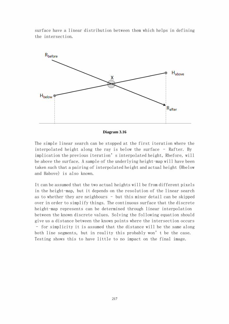
217

surface have a linear distribution between them which helps in defining

the intersection.

Diagram 3.16

The simple linear search can be stopped at the first iteration where the

interpolated height along the ray is below the surface – Rafter. By

implication the previous iteration’s interpolated height, Rbefore, will

be above the surface. A sample of the underlying height-map will have been

taken such that a pairing of interpolated height and actual height (Hbelow

and Habove) is also known.

It can be assumed that the two actual heights will be from different pixels

in the height-map, but it depends on the resolution of the linear search

as to whether they are neighbours – but this minor detail can be skipped

over in order to simplify things. The continuous surface that the discrete

height-map represents can be determined through linear interpolation

between the known discrete values. Solving the following equation should

give us a distance between the known points where the intersection occurs

– for simplicity it is assumed that the distance will be the same along

both line segments, but in reality this probably won’t be the case.

Testing shows this to have little to no impact on the final image.

218

All of the above can be implemented in the following pixel shader:

float3 ray_trace

(

float2 pStart,

float3 vDir,

uniform float HEIGHT_SCALE,

uniform uint MIN_SAMPLES,

uniform uint MAX_SAMPLES,

uniform bool COUNT_SAMPLES_TAKEN

)

{

// Compute initial parallax displacement direction:

float2 vParallaxDirection = normalize( vDir.xy );

// The length of this vector determines the

// furthest amount of displacement:

float fLength = length( vDir );

fLength *= fLength;

float vDirZ_sq = vDir.z * vDir.z;

float fParallaxLength = sqrt( fLength - vDirZ_sq )

219

fParallaxLength /= vDir.z;

// Compute the actual reverse parallax displacement

vector:

float2 vParallaxOffset = vParallaxDirection *

fParallaxLength;

// Need to scale the amount of displacement to account

// for different height ranges in height maps.

vParallaxOffset *= HEIGHT_SCALE;

// corrected for tangent space. Normal is always z=1 in

TS and

// v.viewdir is in tangent space as well...

uint nNumSteps = (int)lerp

(

MAX_SAMPLES,

MIN_SAMPLES,

normalize( vDir ).z

);

float fCurrHeight = 0.0;

float fStepSize = 1.0 / (float) nNumSteps;

uint nStepIndex = 0;

float2 vTexCurrentOffset = pStart;

float2 vTexOffsetPerStep = fStepSize * vParallaxOffset;

float3 rVal = float3

(

vTexCurrentOffset

- ( vTexOffsetPerStep * nNumSteps ),

0.0f

);

float dx = ddx( pStart.x );

float dy = ddy( pStart.y );

float fPrevHeight = 1.0;

float curr_ray_dist = 1.0f;

while ( nStepIndex < nNumSteps )

{

// Determine where along our ray we currently are.

curr_ray_dist -= fStepSize;

220

vTexCurrentOffset -= vTexOffsetPerStep;

fCurrHeight = texHeightMap.SampleGrad

(

DefaultSampler,

vTexCurrentOffset,

dx,

dy

).r;

if( COUNT_SAMPLES_TAKEN )

rVal.z += ( 1.0f / (MAX_SAMPLES - MIN_SAMPLES) );

// Because we're using heights in the [0..1] range

// and the ray is defined in terms of [0..1] scanning

// from top-bottom we can simply compare the surface

// height against the current ray distance.

if ( fCurrHeight >= curr_ray_dist )

{

// Push the counter above the threshold so that

// we exit the loop on the next iteration

nStepIndex = nNumSteps + 1;

// We now know the location along the ray of the

first

// point *BELOW* the surface and the previous point

// *ABOVE* the surface:

float ray_dist_above = curr_ray_dist

+ ( 1.0f / (float)nNumSteps );

float ray_dist_below = curr_ray_dist;

// We also know the height of the surface before

and

// after we intersected it:

float surf_height_before = fPrevHeight;

float surf_height_after = fCurrHeight;

float numerator = ray_dist_above -

surf_height_before;

float denominator =

(surf_height_after - surf_height_before)

- (ray_dist_below - ray_dist_above);

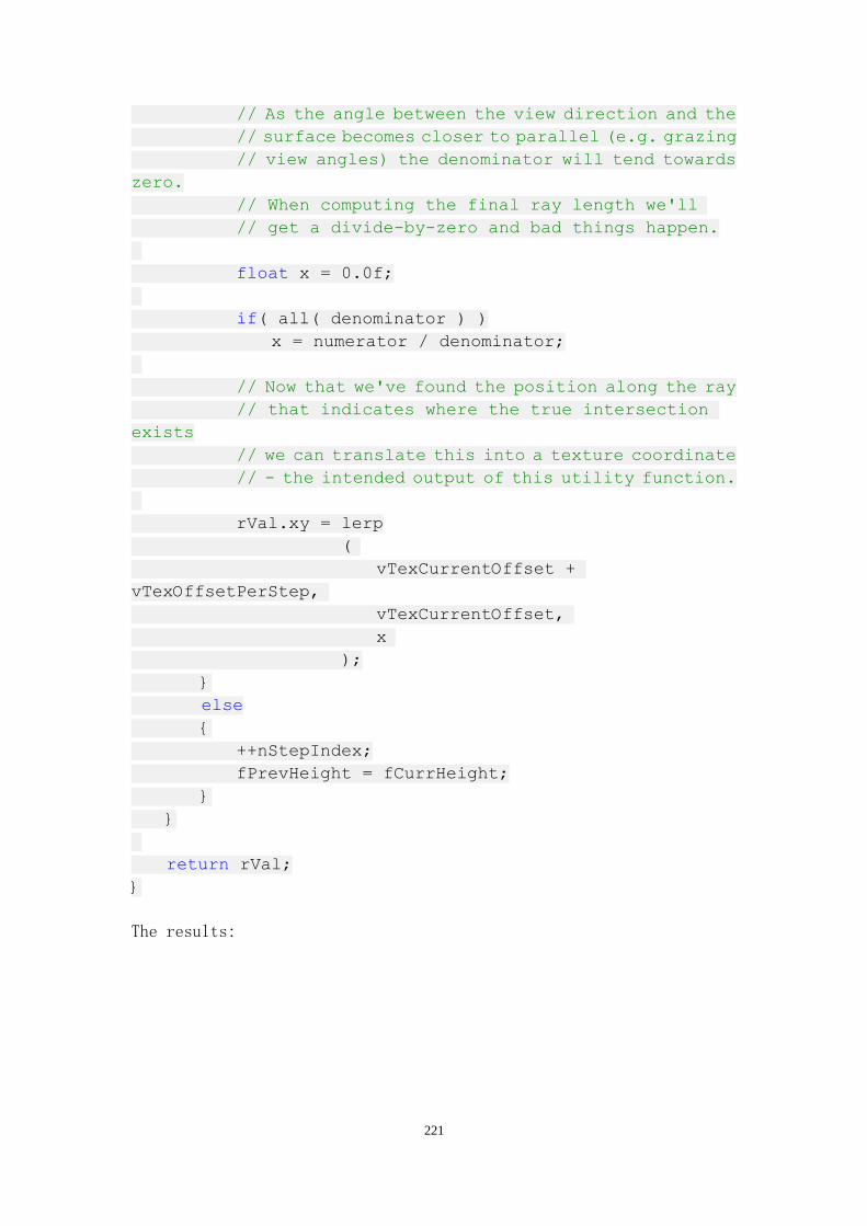
221

// As the angle between the view direction and the

// surface becomes closer to parallel (e.g. grazing

// view angles) the denominator will tend towards

zero.

// When computing the final ray length we'll

// get a divide-by-zero and bad things happen.

float x = 0.0f;

if( all( denominator ) )

x = numerator / denominator;

// Now that we've found the position along the ray

// that indicates where the true intersection

exists

// we can translate this into a texture coordinate

// - the intended output of this utility function.

rVal.xy = lerp

(

vTexCurrentOffset +

vTexOffsetPerStep,

vTexCurrentOffset,

x

);

}

else

{

++nStepIndex;

fPrevHeight = fCurrHeight;

}

}

return rVal;

}

The results:

222

Image 3.17

The following image shows the number of samples required to render the

above screenshot, lighter areas required more samples than darker. The

exact sampling counts can be changed, but in this instance black would

be 15 samples and white would be 75 samples.

223

Image 3.18

Given the previously discussed method for tracing the ray defined by the

view direction it is worth considering that there are actually two rays

that could be considered for this approach:

224

Diagram 3.19

The approach previously discussed can be used to find the point marked

‘Actual’ in diagram 3.19; from here a vector from the light to the

surface intersection can be computed. Tracing along this new vector

reveals an intersection (marked ‘A’ in diagram 3.19) that implies the

fragment currently being rendered receives no light energy due to being

in a shadow.

Exactly the same technique for tracing the ray as before makes it possible

to determine whether the pixel in question is in a shadow cast by another

part of the surface – also known as “self shadowing”. A slightly

modified version of the code can be used for tracing shadows as it is no

longer of any interest where the intersection is – just that there is,

or is not an intersection along the ray. By rearranging the method to

return a simple binary answer the code generated can be much less

complicated and hence faster. The following code shows the refined

ray-tracing method:

float2 vParallaxDirection = normalize( v.lightdir.xy );

float fLength = length( vDir );

fLength *= fLength;

float vDirZ_sq = vDir.z * vDir.z;

float fParallaxLength = sqrt( fLength - vDirZ_sq )

225

fParallaxLength /= vDir.z;

float2 vParallaxOffset = vParallaxDirection *

fParallaxLength;

vParallaxOffset *= HEIGHT_SCALE;

uint nNumSteps = (int)lerp

(

MAX_SAMPLES,

MIN_SAMPLES,

normalize( v.lightdir ).z

);

float fCurrHeight = 0.0;

float fStepSize = 1.0 / (float) nNumSteps;

uint nStepIndex = 0;

float2 vTexCurrentOffset = uv.xy;

float2 vTexOffsetPerStep = fStepSize * vParallaxOffset;

float fCurrentBound = 1.0;

float dx = ddx( v.texcoord.x );

float dy = ddy( v.texcoord.y );

float fPrevHeight = 1.0;

float initial_height = texHeightMap.Sample

(

DefaultSampler,

uv.xy

).r + SHADOW_OFFSET;

if( SHOW_SAMPLE_COUNT )

uv.z += ( 1.0f / ( (MAX_SAMPLES - MIN_SAMPLES) + 1 ) );

while( nStepIndex < nNumSteps )

{

vTexCurrentOffset += vTexOffsetPerStep;

float RayHeight = lerp

(

initial_height,

1.0f,

nStepIndex / nNumSteps

226

);

fCurrHeight = texHeightMap.SampleGrad

(

DefaultSampler,

vTexCurrentOffset,

dx,

dy

).r;

if( SHOW_SAMPLE_COUNT )

uv.z += ( 1.0f / ( (MAX_SAMPLES - MIN_SAMPLES) + 1 ) );

if( fCurrHeight > RayHeight )

{

// ray has gone below the height of the surface,

therefore

// this pixel is occluded...

s = 1.0f;

nStepIndex = nNumSteps;

}

++nStepIndex;

}

As shown in the above code-listing it is necessary to add a small bias

to the height of the ray. Without this bias it is all too easy to introduce

a very noticeable aliasing where pixels are marked as being in shadow when

they shouldn’t be. The cause for this isn’t technically an error but

a case where the test is too accurate. Checking the ray for intersections

can result in it incorrectly identifying the initial pixel as occluding

the ray or if there is a very slight variation with one of its neighbours

(e.g. for an 8 bit height map the origin could have value 150 and the

neighbour 151) . Adding the bias to the calculation generates the results

that we expect as it effectively skips intersections with the original

pixel – correcting the starting location to not sample the original pixel

is an alternative approach but still yields some minor cases of aliasing

that this simple biasing approach manages to avoid.

The following image, 3.20 shows the results of a self-shadowed ray-traced

per-pixel lighting implementation. It is immediately obvious that the

shadowed areas are ‘hard’ – by definition the algorithm only determines

whether a pixel is or is not within shadow. More visually pleasing results

can be achieved by implementing soft shadowing, one method for this is

described in [Tartarchuk06] and is not substantially more difficult or

227

complex to implement. By utilizing the hard self-shadowing approach shown

here it is worth noting that the frequency of the height map becomes a

crucial factor. A low frequency height map contains smooth and gentle

changes in height whereas a high frequency map will have sharp and dramatic

features. The importance is that hard self-shadowing favours a more

high-frequency surface as the hardness of the shadows appears more

visually acceptable; self-shadowing on a low-frequency surface still

works but can look incorrect (regardless of the fact that it is actually

correct!) to the observer. All three of the core algorithms demonstrated

in this chapter favour low- to mid- frequency surfaces for best results,

consequently this means that some degree of testing is essential to ensure

that the final results are acceptable.

Image 3.20

As should be immediately obvious, performing this operation requires

double the work and thus the expense may not seem worthwhile. However,

as will be covered in subsequent chapters of this book it is worth

considering that running a test at this point may well allow execution

to completely skip any implementation of the lighting equation. For the

more complex lighting models that require a huge number of instructions

it may well be a net saving to eliminate them via an initial self-shadowing

test. Then again, as has been previously stressed the advantages of this

228

are largely dependent on the underlying hardware’s implementation of the

high level constructs such as dynamic branching.

Comparison Of Results

This chapter started out by explaining why per-pixel lighting is important

and then proceeded to explain three different methods for achieving the

same thing. This final section compares the results of each of these

techniques and provides a simple summary.

Image 3.21 – Simple Normal Mapping Image 3.22 – Parallax Mapping with Offset

Limiting

Image 3.23 – Ray-Traced Image 3.24 – Ray-Traced with Self-Shadowing

The previous four images were all taken with the same environment settings

and are directly comparable. Simple normal mapping exhibits an almost

annoying behaviour of flipping between raised or depressed bumps

depending on how you look at it – either way it is difficult to extract

the exact shape of the surface being represented. Image 3.22, parallax

mapping with offset limiting, is an improvement and it becomes clear that

229

the surface is made up of a grid of depressions. With the ray-traced

approach there is no doubt as to the surface being represented and the

self-shadowing form reveals a lot about the direction of the light source.

There is a natural progression through the techniques demonstrated in this

chapter: Ray traced parallax with offset limiting, normal mapping and no

per-pixel lighting. [Tartarchuk06] includes the idea of using mip-mapping

to blend between these different methods based on a given pixel’s level

of detail in the final image. If the pixel shader manually computes the

mip-level to be used then it can select a higher or lower quality per-pixel

lighting technique. The basic idea being that the shader scales the

quality of the technique according to the actual contribution to the final

image.

The following table contains a technical summary of each technique. Using

the command-line HLSL compiler it is possible to generate an HTML

formatted assembly code listing (use the /Fc and /Cc parameters) and it

is therefore possible to determine how complex the shader really is. The

values shown in the following table are provided only for guidance

purposes – it is possible to implement some of these techniques with more

or less instructions and the HLSL compiler is often being improved such

that in time the same code might compile to less instructions.

Name Normal

Map?

Height

Map? Instructions Samples

Dynamic

Flow Comments

None No No 2 0 No

Would require additional

geometry to simulate a

more complex surface

Simple Yes No 9 1 No

Good quality results but

can show some unexpected

results

Parallax with

offset Yes Yes 15 2 No

A simple change to the

base algorithm yielding

substantially better results

Ray-traced Yes Yes 68 15-75 Yes Best quality results with a

high computation cost

Ray-traced

with shadows Yes Yes 114 30-150 Yes

Improves upon parallax

occlusion by adding

self-shadowing to the

surface

It is important to realise that the two ray-traced techniques use dynamic

flow control (via looping) and as such the number of instructions executed

230

could be substantially higher than those used to define the program

itself.

Both the parallax and ray-traced approaches utilize a height-map and

therefore become good candidates for run-time normal generation. By

taking this route the number of instructions increases by between 13 and

38 whilst the samples increase by 2 or 7 depending on the technique used.

References

[Blinn78] “Simulation of Wrinked Surfaces”, Computer Graphics

(SIGGRAPH 1978 Proceedings), volume 12, pages 286-292, August 1978.

[Lengyel03] Page 184 of Mathematics for 3D Game Programming & Computer

Graphics 2nd Edition by Eric Lengyel. ISBN 1-58450-277-0.

[Welsh04] “Parallax Mapping with Offset Limiting: A Per-Pixel

Approximation of Uneven Surfaces”, Terry Welsh, January 2004.

[Kaneko01] “Detailed Shape Representation with Parallax Mapping”,

Tomomichi Kaneko, et al. 2001.

[Policarpo05] “Real-Time Relief Mapping on Arbitrary Polygonal

Surfaces”, Policarpo, Oliveira and Comba, 2005.

[Tartarchuk06] “Practical parallax occlusion mapping for highly

detailed surface rendering”, Natalya Tartarchuk, ATI Research,

Presented at the Game Developers Conference 2006.

Phong and Blinn-Phong

Lighting models are not a new aspect of computer graphics and research

has been on-going for several decades. The model proposed by Phong

Bui-Tuong is possibly one of the oldest and arguably the most classic model

still in use today. Whilst not as sophisticated as the models described

in the following chapters it is very simple to implement, has good

performance characteristics and generates acceptable results.

This chapter covers a modification to the original model – that proposed

by James Blinn. He put forward a simplified version of Phong’s original

equation that has even better performance yet minimal effect on the final

result. Several sources will claim James Blinn’s modifications as an

approximation to Phong Bui-Tuong’s but a recently published paper ([Ngan


231

et al. 04]) claims otherwise: James Blinn’s modifications match measured

data more accurately than Phong Bui-Tuong’s model.

These simplifications along with equivalent or better quality have

effectively made the Blinn-Phong form the baseline lighting model for

three decades.

Developers familiar with the fixed-function lighting pipeline from

previous versions of Direct3D will be familiar with the results as the

Blinn-Phong model is. Obviously the fixed-function pipeline has now been

removed, but the SDK ships with the “FixedFuncEmu” sample that

implements the entire functionality of this legacy pipeline in terms of

the Direct3D 10’s shader model 4. Looking through this SDK sample it is

possible to find an implementation of the Blinn-Phong lighting model in

the CalcLighting() function inside FixedFuncEMU.fx.

The Phong Equation

In the “Foundation and Theory” chapter the Lambertian N•L factor was

introduced – this works fine for simple diffuse lighting terms where

light energy is distributed evenly across the hemisphere defined by the

surface and its normal vector. Diffuse lighting is independent of the

observer’s position relative to the surface. However this does not work

for another class of light reflectance – specular. Phong Bui Tuong’s

1973 model ([Phong73]) introduces this term for improved realism.

Specular lighting is effectively the opposite of diffuse lighting as it

only reflects light energy in the mirror direction.

The Phong equation computes the reflection of the incoming light energy

about the surface normal, therefore modelling the fact that specular light

has a particular distribution function. This reflected light energy will

only be picked up by the observer if the view direction corresponds to

the region defined by this distribution function and therefore makes it

a view-dependent result. Ultimately this leads to brighter highlights on

the final image – perfect for representing shiny materials.

232

Diagram 4.1

The trusty dot-product operation can be used to determine the relationship

between the observer and the reflected light energy but it is not quite

enough for the desired results. Diagram 4.1 shows three different shapes

for the reflected light – the specular highlight will only appear in the

final image if the view direction intersects with the volume shown.

Normally the dot-product will work for the full hemisphere defined by the

vector (assuming we clamp it to 0.0-1.0 in the same way as the Lambertian

term does) but we need to raise the dot product to a power in order to

change the effective ‘range’ of the dot-product.

What diagram 4.1 is really showing is three different exponents – the

variable employed by Phong’s equation to allow for a much wider range

of materials to be represented. A high exponent (e.g. 50) will result in

very sharp, small highlights whereas a low value (e.g. 5) will give much

softer and larger highlights. There are no fixed rules for the value to

be used – rather it is down to artistic license and choosing a value that

looks appropriate.

Mathematically the Phong equation looks like this:

When implemented in HLSL it looks like this:

float4 phong( in float3 normal, in float3 viewer, in float3

light )

{

// Compute the reflection vector

float3 reflection = normalize( 2.0f * normal *

dot( normal, light ) - light );

233

// Compute the angle between the reflection and the viewer

float RdotV = max( dot( reflection, viewer ),

0.0f );

// Compute the specular colour

float3 specular = cSpecular * pow( RdotV,

fSpecularExponent );

// Compute the diffuse term for the Phong equation

float3 diffuse = cDiffuse * max( 0.0f, dot( normal,

light ) );

// Determine the final colour

return float4( diffuse + specular, 1.0f );

}

The Blinn-Phong Equation

Whilst the reflection vector used to compute the specular term in Phong’s

original equation has mathematical correctness it is possible to simplify

it (and, as previously discussed, more accurately match real-world data).

James Blinn’s paper ([Blinn77]) shows that by replacing the reflection

vector with a ‘half’ vector it is possible to generate results close

to the original model but with a more favourable performance profile. Keep

in mind that the HLSL code shown previously will be executed for every

single pixel rasterized with this pipeline configuration – shaving even

a few instructions can result in millions less executed when scaled up

by the number of times the pixel shader is invoked.

Diagram 4.2

234

Using simple vector mathematics it is possible to compute the “half

vector” between the light and view direction. Diagram 4.2 shows how this

compares with the other vectors – in the incident plane the angles marked

(θ ) are related, but in the more general case (over the hemisphere in

3D) the relationship is much more complicated which gives rise to the more

accurate match against real-world data.

The modified equation is therefore:

When implemented in HLSL appears as:

float4 blinn_phong( in float3 normal, in float3 viewer, in

float3 light )

{

// Compute the half vector

float3 half_vector = normalize(light + viewer);

// Compute the angle between the half vector and normal

float HdotN = max( 0.0f, dot( half_vector, normal ) );

// Compute the specular colour

float3 specular = cSpecular * pow( HdotN,

fSpecularExponent );

// Compute the diffuse term

float3 diffuse = cDiffuse * max( 0.0f, dot( normal,

light ) );

// Determine the final colour


}

235

Results

Image 4.3

The main input into both forms of this lighting model is the specular

exponent which, when used well, can provide a substantial degree of

flexibility. The above image shows the same sphere lit with the Phong model

(top) and Blinn-Phong (bottom) with exponents of 1 (left), 15, 30 and 100

(right).

It is immediately obvious that the two models are quite different given

the same inputs – there is no hard rule, but generally speaking the

Blinn-Phong model requires an exponent around four times higher than

Phong’s original equation to generate similar results.

As shown in both equations the diffuse and specular terms are scaled by

constant colour values. Typically these constants would be fetched from

textures bound to the pipeline and thus vary on a per-pixel basis. This

puts a degree of responsibility on the artist to select appropriate values

as unrealistic results might be generated if the incoming constants are

too high. By allowing full control over the terms it is possible to

represent both homogenous and non-homogenous materials (as explained in

the first chapter of this section) with no changes to the code.

Whilst it might be more appropriate to measure frame-times and perform

more standard benchmarks the results of these are highly specific to the

underlying hardware and software such that it becomes very difficult to

draw meaningful conclusions. Instead, a useful measure of the performance

improvement is to look at the assembly complexity of the two techniques.

By using the command-line HLSL compiler it is possible to generate a

colour-coded HTML assembly listing.

The original Phong equation gets compiled to 26 instructions whereas the

Blinn-Phong equation gets compiled to 23 instructions – a saving of 3.

236

This may not sound like much but, referring back to the previous point

about the number of pixel shader invocations consider the following image:

Image 4.4

The preceding image was rendered at 640x480 and thus has 307,200 pixels

in total. A crude estimate using histograms shows that the model being

rendered occupies 100,000 of those pixels. A saving of 3 instructions

yields around 300,000 fewer instructions being executed per frame, which

at the captured frame rate is 97.5 million fewer per second.

The Phong and Blinn-Phong models are good general-purpose lighting models

as demonstrated by their adoption as standard in the ‘fixed function’

Direct3D pipeline. However their simplicity can reduce their

applicability when representing some materials – more complex effects

like the Fresnel term can make a substantial impact. A common observation

is that these models give models a plastic-like appearance.

237

References

[Ngan et al. 04] “Experimental Validation of Analytical BRDF Models.”

Addy Ngan, Fredo Durand & Wojciech Matusik. Technical Sketch, Siggraph

2004

[Phong73] “Illumination for Computer Generated Images” 1973, or

“Illumination for computer generated pictures” ACM June 1975

[Blinn77] “Models of Light Reflection for Computer Synthesized

Pictures”, James F. Blinn, ACM Siggraph ’77 Conference Proceedings

Cook-Torrance

A common problem with the Phong and Blinn-Phong models discussed in the

previous chapter is that they look too artificial. Whilst they are general

purpose in design a number of simplifications means that a lot of the

subtleties of materials cannot be represented. The model discussed

throughout this chapter was published by Robert Cook and Kenneth Torrance

in 1982 ([Cook&Torrance82]) – a few years after James Blinn published

his modifications to Phong’s original model.

The Cook-Torrance lighting model is a general model for rough surfaces

and is targeted at metals and plastics – although it is still possible

to represent many other materials. The model is still split into two

distinct terms – diffuse and specular – as was true of the previous model

(and for those discussed in later chapters); the key difference is the

computation of the specular term.

Phong’s model uses simple mathematical principles of reflection to

determine how much, if any, of a specular highlight is visible. Whilst

the colour of this highlight can be varied as a per-pixel input into the

equation it is a constant colour from all angles regardless of the viewing

direction. The Cook-Torrance model details a more complex and accurate

way of computing the colour of the specular term – an approach based more

on physics than pure mathematics.

238

The Cook-Torrance Equation

This equation is much more involved than the simpler Phong-based equations

of the previous chapter. Despite this the equation can be neatly

summarised as follows:

As previously discussed the key differentiator in the Cook-Torrance

equation is the specular term, Rs. The remainder of this section will focus

on this term and specifically work through the three main components

making up its numerator – Fresnel, roughness and geometric.

Modelling a rough surface might seem possible by using a high resolution

per-pixel normal map (as discussed in chapter 3) but this doesn’t tend

to yield the desired results. Cook-Torrance adopted the “Microfacet”

method for describing the roughness of a given surface:

Diagram 5.1

The microfacets are intended to be smaller than can be displayed on the

screen; rather it is the combined effect across the entire surface that

shows the roughness. Constants can be used to control the depth and size

of these facets and thus control the perceived roughness of the surface.

The implementation in this chapter sets these constants on a per-material

239

basis but it is perfectly possible to store per-pixel roughness

coefficients so as to allow for a much higher degree of variation.

Half vectors introduced as part of the Blinn-Phong model make an

appearance in the Cook-Torrance model. In much the same way as with

Blinn-Phong, the reflected specular energy is defined about this vector

rather than the reflection vector as in the original Phong equation.

The geometric term

In the original paper ‘Geometric Attenuation’ is a product of two

effects – shadowing and masking. Fundamentally they are the same effect,

but one caters for incoming energy and the other for outgoing energy.

Shadowing can be referred to as ‘self shadowing’ – a term quite commonly

used for several currently popular algorithms. Diagram 5.2 shows how

incoming light energy can be blocked by its own, or a neighbouring, facet:

Diagram 5.2

The other factor, masking, is very similar but covers the possibility that

the reflected light is blocked by the facet. Diagram 5.3 illustrates this:

240

Diagram 5.3

Given that these microfacets are supposed to be extremely small it might

seem irrelevant that they block light energy, but it is a very important

factor in the final image. Shadowing and masking increases with the depth

of the microfacets leading to very rough surfaces being quite dull or matt

in appearance.

The following equation can be used to compute the geometric term:

The Roughness Term

This factor is a distribution function to determine the proportion of

facets that are oriented in the same direction as the half vector. Only

facets facing in this direction will contribute to reflected energy and

a simple observation of modelling a rough surface is that not all of the

surface will be facing in the same direction. As the surface becomes

rougher it is more likely that parts of the surface will be oriented away

from the half vector.

Various distributions have been experimented with for this component of

the Cook-Torrance model. Many models aim to reproduce the wavelength

241

scattering measured from specific real-world rough materials and tend to

be very complicated albeit much more physically accurate.

When graphed, these distribution functions appear to be similar to the

specular distribution used in the Phong model; light energy is scattered

within a volume about the reflected vector. For a very smooth surface this

distribution is concentrated about the reflected vector and yields a very

sharp highlight, for a rough surface the distribution is much wider due

to the roughness scattering light energy in many different directions.

The smooth-surface case is very similar to that modelled by Phong.

Diagram 5.4

Beckmann’s distribution ([Beckmann&Spizzichino63]) covers a wide range

of materials of varying roughness with considerable accuracy; the main

trade-off is that it is a complex distribution to evaluate and thus not

so suitable for performance-intensive usage.

The above equation can be converted to vector form so as to eliminate the

two trigonometric functions. α is defined as being the angle between the

normal vector and the half vector. This makes the equation much more

suitable for implementation in a pixel shader:

242

It is also worth considering that this distribution could be stored in

a texture as a look-up table (a method suggested in the first chapter of

this section). Using <Normal•Half, m2> as a 2D texture coordinate will

allow a single texture sample to replace the entire evaluation of this

distribution. The following code can be used to create the look-up

texture:

HRESULT CreateRoughnessLookupTexture( ID3D10Device*

pDevice )

{

HRESULT hr = S_OK;

// The dimension value becomes a trade-off between

// quality and storage requirements

const UINT LOOKUP_DIMENSION = 512;

// Describe the texture

D3D10_TEXTURE2D_DESC texDesc;

texDesc.ArraySize = 1;

texDesc.BindFlags =


texDesc.CPUAccessFlags = 0;

texDesc.Format = DXGI_FORMAT_R32_FLOAT;

texDesc.Height = LOOKUP_DIMENSION;

texDesc.Width = LOOKUP_DIMENSION;

texDesc.MipLevels = 1;

243

texDesc.MiscFlags = 0;

texDesc.SampleDesc.Count = 1;

texDesc.SampleDesc.Quality = 0;

texDesc.Usage = D3D10_USAGE_IMMUTABLE;

// Generate the initial data

float* fLookup = new

float[ LOOKUP_DIMENSION*LOOKUP_DIMENSION ];

for( UINT x = 0; x < LOOKUP_DIMENSION; ++x )

{

for( UINT y = 0; y < LOOKUP_DIMENSION; ++y )

{

// This following fragment is a direct conversion

of

// the code that appears in the HLSL shader

float NdotH = static_cast< float >( x )

/ static_cast<

float >( LOOKUP_DIMENSION );

float Roughness = static_cast< float >( y )

/ static_cast<


// Convert the 0.0..1.0 ranges to be -1.0..+1.0

NdotH *= 2.0f;

NdotH -= 1.0f;

// Evaluate a Beckmann distribution for this

element

// of the look-up table:

float r_sq = Roughness * Roughness;

float r_a = 1.0f / ( 4.0f * r_sq * pow( NdotH, 4 ) );

float r_b = NdotH * NdotH - 1.0f;

float r_c = r_sq * NdotH * NdotH;

fLookup[ x + y * LOOKUP_DIMENSION ]

= r_a * expf( r_b / r_c );

}

}

D3D10_SUBRESOURCE_DATA initialData;

initialData.pSysMem = fLookup;

initialData.SysMemPitch = sizeof(float) *

LOOKUP_DIMENSION;

244

initialData.SysMemSlicePitch = 0;

// Create the actual texture

hr = pDevice->CreateTexture2D

(

&texDesc,

&initialData,

&g_pRoughnessLookUpTex

);

if( FAILED( hr ) )

{

ERR_OUT( L"Failed to create look-up texture" );

SAFE_DELETE_ARRAY( fLookup );

return hr;

}

// Create a view onto the texture

ID3D10ShaderResourceView* pLookupRV = NULL;

hr = pDevice->CreateShaderResourceView

(

g_pRoughnessLookUpTex,

NULL,

&pLookupRV

);

if( FAILED( hr ) )

{

SAFE_RELEASE( pLookupRV );

SAFE_RELEASE( g_pRoughnessLookUpTex );


return hr;

}

// Bind it to the effect variable

ID3D10EffectShaderResourceVariable *pFXVar

=

g_pEffect->GetVariableByName("texRoughness")->AsShaderRes

ource( );

if( !pFXVar->IsValid() )

{


245

SAFE_RELEASE( g_pRoughnessLookUpTex );


return hr;

}

pFXVar->SetResource( pLookupRV );

// Clear up any intermediary resources



return hr;

}

James Blinn proposed the use of a standard Gaussian distribution:

This distribution is not as physically accurate as Beckmann’s

distribution but in a lot of scenarios the approximation will be perfectly

acceptable. Evaluation of the Gaussian distribution is much easier than

Beckmann’s thus making the approximation a compelling option for

real-time use. The only potential problem of the Gaussian distribution

is that it relies on an arbitrary constant that needs to be empirically

determined for best results.

The Fresnel Term

An important part of the Cook-Torrance model is that the reflected

specular light is not a constant colour; rather it is view-dependent. The

Fresnel term, introduced in the first chapter of this section, can be used

to model this characteristic.

The full Fresnel equation is overly complicated for this purpose and

relies on expensive and complex evaluation. The original publication

contains the full equations along with useful derivations regarding

source data. However it is worth noting that any measurement used in

Fresnel evaluations is dependent on numerous physical properties such as

the wavelength of light and temperature. It depends on the intended usage

whether modelling these characteristics is worth the additional

complexity. For real-time computer graphics it is generally more suitable

to use an approximation presented by Christophe Schlick ([Schlick94]).

246

In the above approximation F0 is the Fresnel reflectance as measured at

normal incidence. Available Fresnel information is typically expressed

in this form which makes it a convenient parameter to work with.

Schlick’s approximation is simply a nonlinear interpolation between the

refraction at normal incidence and total reflection at grazing angles.

Implementation

The previous section covered the components of the Cook-Torrance lighting

model. The following list summarises each of these parts in the order of

which they must be evaluated:

1. Compute geometric term

2. Compute roughness term using one of the following options:

2a Sample from a texture generated by the application – distribution

becomes unimportant. [Texture2D look-up and roughness value required]

2b Evaluate with the Beckmann Distribution [roughness value required]

2c Evaluate with a Gaussian Distribution [roughness value and arbitrary

constant required]

3 Compute the Fresnel term

3a Evaluate Christophe Schlick’s approximation [Requires index of

refraction]

4 Evaluate Rs term of the full equation:

247

5 Evaluate complete equation

The above series of steps when implemented in HLSL is as follows, note

that this is a single HLSL function that relies on conditional compilation

to split into different techniques; this is a valuable technique for code

re-use and maintenance but arguably it can make the code less intuitive

to read:

float4 cook_torrance

(

in float3 normal,

in float3 viewer,

in float3 light,

uniform int roughness_mode

)

{

// Compute any aliases and intermediary values

// -------------------------------------------

float3 half_vector = normalize( light + viewer );

float NdotL = saturate( dot( normal, light ) );

float NdotH = saturate( dot( normal,

half_vector ) );

float NdotV = saturate( dot( normal, viewer ) );

float VdotH = saturate( dot( viewer,

half_vector ) );

float r_sq = roughness_value * roughness_value;

// Evaluate the geometric term

// --------------------------------

float geo_numerator = 2.0f * NdotH;

float geo_denominator = VdotH;

float geo_b = (geo_numerator * NdotV ) / geo_denominator;

float geo_c = (geo_numerator * NdotL ) / geo_denominator;

float geo = min( 1.0f, min( geo_b, geo_c ) );

// Now evaluate the roughness term

// -------------------------------

float roughness;

248

if( ROUGHNESS_LOOK_UP == roughness_mode )

{

// texture coordinate is:

float2 tc = { NdotH, roughness_value };

// Remap the NdotH value to be 0.0-1.0

// instead of -1.0..+1.0

tc.x += 1.0f;

tc.x /= 2.0f;

// look up the coefficient from the texture:

roughness = texRoughness.Sample( sampRoughness, tc );

}

if( ROUGHNESS_BECKMANN == roughness_mode )

{

float roughness_a = 1.0f / ( 4.0f * r_sq * pow( NdotH,

4 ) );

float roughness_b = NdotH * NdotH - 1.0f;

float roughness_c = r_sq * NdotH * NdotH;

roughness = roughness_a * exp( roughness_b /

roughness_c );

}

if( ROUGHNESS_GAUSSIAN == roughness_mode )

{

// This variable could be exposed as a variable

// for the application to control:

float c = 1.0f;

float alpha = acos( dot( normal, half_vector ) );

roughness = c * exp( -( alpha / r_sq ) );

}

// Next evaluate the Fresnel value

// -------------------------------

float fresnel = pow( 1.0f - VdotH, 5.0f );

fresnel *= ( 1.0f - ref_at_norm_incidence );

fresnel += ref_at_norm_incidence;

// Put all the terms together to compute

249

// the specular term in the equation

// -------------------------------------

float3 Rs_numerator = ( fresnel * geo * roughness );

float Rs_denominator = NdotV * NdotL;

float3 Rs = Rs_numerator/ Rs_denominator;

// Put all the parts together to generate

// the final colour

// --------------------------------------

float3 final = max(0.0f, NdotL) * (cSpecular * Rs +

cDiffuse);

// Return the result

// -----------------

return float4( final, 1.0f );

}

Results

Image 5.5

The above image shows the Beckmann distribution (top) and Gaussian

distribution (bottom) with roughness values of 0.2 (left), 0.4, 0.6, 0.8

and 1.0 (right). Whilst the Gaussian form is noticeably different to the

Beckmann form it is worth noting that there is an arbitrary constant

controlling the Gaussian distribution. Experimentation with this

coefficient can generate closer or more visually acceptable results.

250

Image 5.6

The two key inputs into the Cook-Torrance model are reflectance at normal

incidence and roughness. Image 5.6 serves to show their relationship and

the types of results that can be achieved.

It should come as no surprise that low roughness values, implying a smooth

surface, generate the shiniest results with specular highlights similar

to that seen with the Phong model. Experimentation for achieving other

materials is necessary, but from Image 5.6 it should be apparent that the

Cook-Torrance model spans a large number of possibilities; the range shown

in the image is representative but does not display the extreme values

– lower or higher inputs are allowed.

The assembly code emitted by the HLSL compiler for the Cook-Torrance model

yields some surprising results. In particular the Gaussian roughness

distribution compiles to more instructions than the Beckmann distribution

– given that the motivation behind the Gaussian distribution was its

simple implementation!

Using a look-up texture shaves around 16% off the instruction count, which

is a worthwhile saving provided there aren’t any problems with using an

extra 1-2mb of video memory.

251

References

[Cook&Torrance82] “A Reflectance Model for Computer Graphics” ACM

Transactions on Graphics, volume 1, number 1, January 1982 pages 7-24

[Schlick94] “An inexpensive BRDF model for physically-based

rendering.” Christophe Schlick, Computer Graphics Forum, 13(3):233—246,

1994.

[Beckmann&Spizzichino63] “The scattering of electromagnetic waves from

rough surfaces.” MacMillan, New York, 1963, pages 1-33 and 70-98.

Oren-Nayar

The lighting model put forward by Michael Oren and Shree Nayar in their

1994 paper is a substantial departure from the previous three. Not only

does it deviate from the otherwise standard Lambertian model but it is

also a diffuse-only model and doesn’t focus on modelling specular

highlights.

This model is particularly useful as it specialises in rough surfaces –

such as brick, concrete and also clothing materials such as velvet. A key

characteristic of a rough surface is the degree of light scattering due

to the uneven surface; this gives rise to several observable qualities

that cannot be replicated using the more traditional lighting models.

Consider the full moon when viewed on a clear night. In this situation

its shape is circular and has a very clearly defined edge when seen against

the background of space. However we know that the moon is a spherical body

and that towards the edge of the full moon its surface is orienting away

from our point of view and the light source. Using a standard Lambertian

approach, the basis for previous models, this would mean that the edge

of the full moon should tend towards darkness – but this is quite clearly

not the case! The following image shows a comparison with a Lambertian

sphere on the left and a rough sphere on the right.

252

Image 6.1

This deviation is down to the scattering of light from a rough surface

– all of the tiny imperfections scatter and reflect light in many more

directions than a smooth surface might. The previous chapter covering the

Cook-Torrance model introduced the idea of ‘micro-facets’ and this

concept provides a foundation for the Oren-Nayar model.

Despite the model breaking Lambertian norms, each micro-facet on the

surface is assumed to show Lambertian reflection; it is the interaction

of these facets that allows the overall result to deviate. The previous

chapter covered distribution functions and self-shadowing and this model

introduces the concept of inter-reflection.

Diagram 6.2

253

The preceding diagram shows a situation where a facet receiving no direct

light is viewed. On the left, where no inter-reflection is considered,

the observed facet is dark and unlit. On the right the facet indirectly

receives light energy due to inter-reflection and consequently appears

lit to the viewer. This effect is most noticeable on rough surfaces because

smooth surfaces have small, if any, facets to generate inter-reflection.

For rough surfaces it is quite possible for the visible side of a facet

to be oriented away from the light source yet its opposite and invisible

side to be oriented towards the light source. By assuming that the lit

side reflects some of the received light energy the visible side of the

facet will in turn reflect some light energy back towards the viewer.

As will become evident over the remainder of this chapter this model is

one of the more complex to implement simply due to the heavy use of

spherical coordinates and trigonometric functions. This doesn’t

invalidate it as an option for real-time computer graphics; rather it

requires consideration regarding its usage. In simple terms it should be

used sparingly and only where the extra computation expense is going to

have a significant influence on the final image.

The Oren-Nayar Equation

The previous Cook-Torrance model is easy to break down into constituent

parts, but unfortunately the rendering equations proposed by Oren-Nayar

is more monolithic. Spherical coordinates are used in the original

equations as they offer numerous mathematical advantages, however for

implementation purposes this is inconvenient – most Direct3D graphics

will be based on the Cartesian coordinate system. The next section of this

chapter demonstrates how it is possible to convert to a more

shader-friendly vector form.

Unit vectors in Cartesian form require three components – x, y and z.

Due to their length being exactly 1.0 they can be represented by only two

values when using spherical coordinates – θ and Φ . Conversion can be

performed according to the following equations:

φ = cos − 1z

The Oren-Nayar equation takes the following values as input:

254

Φi, θi Light‟s direction vector

Φr, θr View direction vector

σ Roughness coefficient, between 0.0 and 1.0

E0 Incoming light energy

ρ/π Diffuse colour for the current pixel

The complete equation, broken down in order to make it easier to read in

printed form, is as follows:

Evaluating the above equation in full will require six calls to

trigonometric functions (three cosines, two tangents and one sine). This,

combined with the possibility of converting Cartesian input vectors into

spherical coordinates makes it a very complex evaluation and definitely

not the most performance-friendly!

255

Due to the computation complexity of the previous equation Oren and Nayar

proposed a simplification as part of the same publication. As with most

simplifications this sacrifices quality and accuracy, but this

qualitative model was arrived at by studying the significance of the many

terms in the previous equation. Both C3 and inter-reflection proved to

have a minimal effect on the final image yet were responsible for a

substantial amount of the computation – the following simplified

equation is based on the removal of these two terms:

The A and B terms are directly derived from C1 and C2 in the original

lighting model. An oft-missed footnote in the original paper suggests that

replacing the 0.33 constant in the original C1 equation with 0.57 can

improve the quality slightly.

It is immediately obvious that this simplification has removed a lot of

the work required for the original model. The simplified model still

depends on four trigonometric functions, but as will be shown in the

following section it is possible to further reduce this.

Implementation

As previously shown, the equations are heavy on spherical coordinates and

trigonometry. This doesn’t suit GPU’s such that it is better to convert

to vector form where possible

Common terms in vector form:

256

The circular angle, γ , can be converted into vector mathematics by

projecting the two angles onto the x,y plane in tangent space. When dealing

with unit vectors it is standard to replace the cosine function with a

much simpler dot-product operation. The full equation in vector form:

The above equations when implemented in HLSL are as follows:

float4 psOrenNayarComplex( in VS_OUTPUT f ) : SV_TARGET

{

const float PI = 3.14159f;

// Make sure the interpolated inputs and

// constant parameters are normalized

257

float3 n = normalize( f.normal );

float3 l = normalize( -vLightDirection );

float3 v = normalize( pCameraPosition - f.world );

// Compute the other aliases

float alpha = max( acos( dot( v, n ) ), acos( dot( l,

n ) ) );

float beta = min( acos( dot( v, n ) ), acos( dot( l,

n ) ) );

float gamma = dot( v - n * dot( v, n ), l - n * dot( l,

n ) );

float rough_sq = fRoughness * fRoughness;

float C1 = 1.0f - 0.5f * ( rough_sq / ( rough_sq +

0.33f ) );

float C2 = 0.45f * ( rough_sq / ( rough_sq + 0.09 ) );

if( gamma >= 0 )

{

C2 *= sin( alpha );

}

else

{

C2 *= ( sin( alpha ) - pow( (2 * beta) / PI, 3 ) );

}

float C3 = (1.0f / 8.0f) ;

C3 *= ( rough_sq / ( rough_sq + 0.09f ) );

C3 *= pow( ( 4.0f * alpha * beta ) / (PI * PI), 2 );

float A = gamma * C2 * tan( beta );

float B = (1 - abs( gamma )) * C3 * tan( (alpha + beta)

/ 2.0f );

float3 final = cDiffuse * max( 0.0f, dot( n, l ) ) * ( C1

+ A + B );

return float4( final, 1.0f );

}

Evaluation of the C2 term requires the use of a dynamic branch in the shader

code which is not ideal. Use of the [branch] and [flatten] attributes can

push the compiler in either direction, but the compiled shader code may

well end up evaluating both branches in order to achieve this.

258

The simplified equation in vector form is straight-forward and still

relies on the previous conversions of α , β and γ :

Implemented in HLSL:

float4 psOrenNayarSimple

(

in VS_OUTPUT f,

uniform bool UseLookUpTexture

) : SV_TARGET

{






// Compute the other aliases

float gamma = dot

(

v - n * dot( v, n ),

l - n * dot( l, n )

);

float rough_sq = fRoughness * fRoughness;

float A = 1.0f - 0.5f * (rough_sq / (rough_sq + 0.57f));

float B = 0.45f * (rough_sq / (rough_sq + 0.09));

float C;

if( UseLookUpTexture )

{

// The two dot-products will be in the range of

259

// 0.0 to 1.0 which is perfect for a texture lookup:

float tc = float2

(

(VdotN + 1.0f) / 2.0f,

(LdotN + 1.0f) / 2.0f

);

C = texSinTanLookup.Sample( DefaultSampler, tc ).r;

}

else

{

float alpha = max( acos( dot( v, n ) ), acos( dot( l,

n ) ) );

float beta = min( acos( dot( v, n ) ), acos( dot( l,

n ) ) );

C = sin(alpha) * tan(beta);

}

float3 final = (A + B * max( 0.0f, gamma ) * C);

return float4( cDiffuse * max( 0.0f, dot( n, l ) ) * final,

1.0f );

}

Both full and simplified still rely on the sin()/tan() terms. The

simplified form of the model makes it trivial to factor out these expensive

operations and replace them with a single texture fetch, as shown by the

presence of the compile-time switch in the above HLSL code. The following

function from the main application shows how to generate the look-up

texture referenced by the HLSL:

HRESULT CreateSinTanLookupTexture( ID3D10Device* pDevice )

{

HRESULT hr = S_OK;

// The incoming dot-product will be between 0.0 and 1.0

// covering 180 degrees thus a look-up of 512 pixels

// gives roughly 1/3rd of a degree accuracy which

// should be enough...





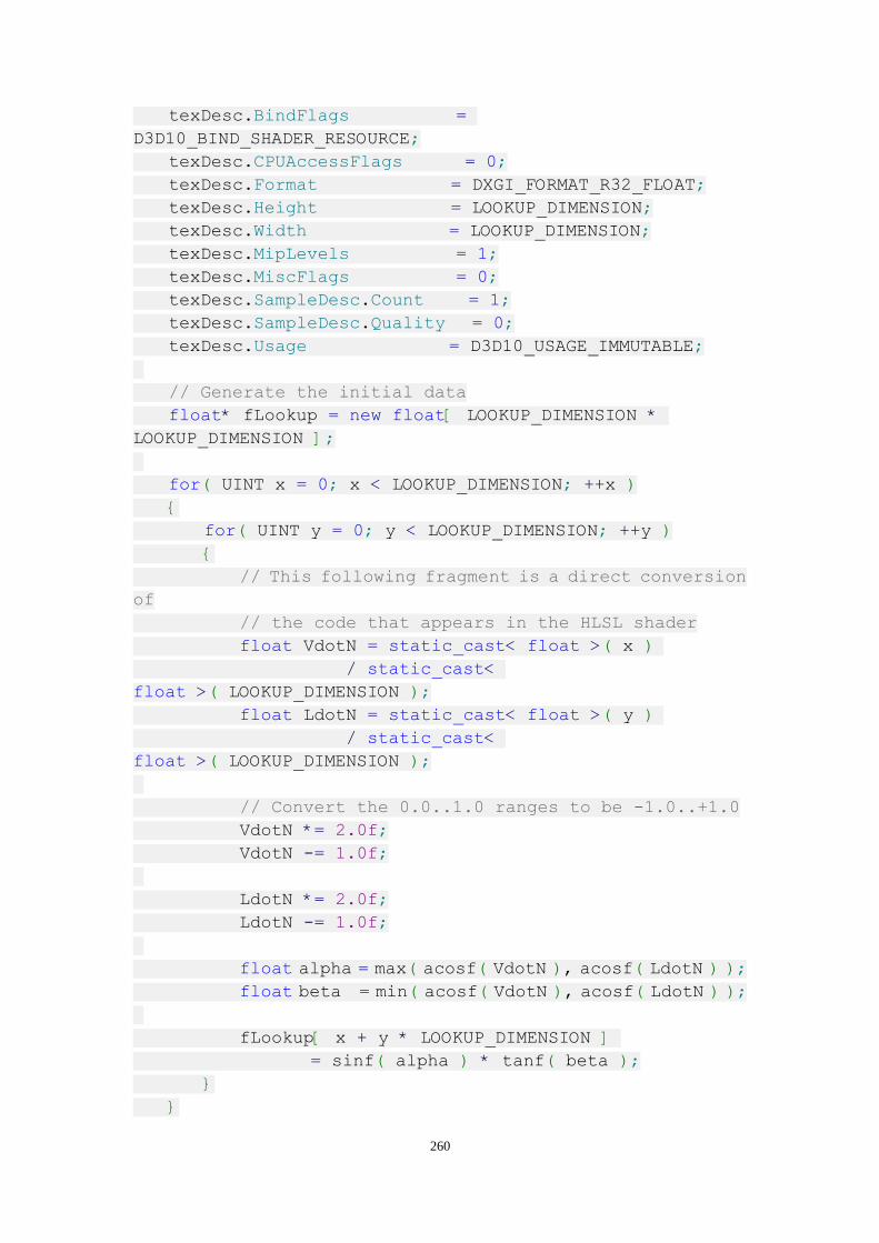
260

texDesc.BindFlags =




texDesc.Height = LOOKUP_DIMENSION;








float* fLookup = new float[ LOOKUP_DIMENSION *

LOOKUP_DIMENSION ];


{

for( UINT y = 0; y < LOOKUP_DIMENSION; ++y )

{


of


float VdotN = static_cast< float >( x )

/ static_cast<


float LdotN = static_cast< float >( y )

/ static_cast<


// Convert the 0.0..1.0 ranges to be -1.0..+1.0

VdotN *= 2.0f;

VdotN -= 1.0f;

LdotN *= 2.0f;

LdotN -= 1.0f;

float alpha = max( acosf( VdotN ), acosf( LdotN ) );

float beta = min( acosf( VdotN ), acosf( LdotN ) );

fLookup[ x + y * LOOKUP_DIMENSION ]

= sinf( alpha ) * tanf( beta );

}

}

261




LOOKUP_DIMENSION;




(

&texDesc,

&initialData,

&g_pSinTanTexture

);

if( FAILED( hr ) )

{


return hr;

}




(

g_pSinTanTexture,

NULL,

&pLookupRV

);

if( FAILED( hr ) )

{


SAFE_RELEASE( g_pSinTanTexture );


return hr;

}



=

g_pEffect->GetVariableByName("texSinTanLookup")->AsShader

Resource( );

262


{


SAFE_RELEASE( g_pSinTanTexture );


return hr;

}





return hr;

}

With some work it would be possible to apply this same principle to the

original and more complex Oren-Nayar equations, but there are less obvious

choices. For example, many of the expensive evaluations require three

inputs which would require a volume texture to be used as a look-up –

something that isn’t good for storage (a low-quality volume texture of

128x128x128 and stored at half-precision still requires 4mb, which is four

times as much as the reasonable quality look-up generated in the above

fragment of code).

Results

Roughness is the key parameter affecting the output from the Oren-Nayar

model. The following set of images show the two main techniques compared

at various roughness coefficients:

263

Image 6.3

As is noted in their paper, when roughness is 0.0 (a completely smooth

surface) the model exhibits Lambertian behaviour in the same way as other

lighting models discussed in this section.

It is difficult to find any visual differences between the complex model

and its simplified form – testament to the fact that the removed terms

didn’t make a significant contribution to the outcome. The most obvious

difference is that the simplified model comes across as being brighter,

but the distribution of light is still the same. It may well be possible

to find some examples where the complex model generates significantly

better results, but for the most part it would be safe to work with the

simplified model unless it showed any obvious signs of incorrectness.

264

Despite the visual differences being negligible the compiled output is

substantially different – the original complex form is 24% longer than

the simplified one. The instruction count drops from 77 to 62 between them

which is surprising given their near-equal results. The use of a texture

look-up knocks 24 instructions off the simplified model bringing it to

a total of 38.

A simple count of instructions can be a useful measure of the evaluation

cost for a shader but it should come as no surprise that individual

instructions will have different costs. Ten expensive instructions may

well be slower than twenty cheap ones even though the latter appears to

be twice as long on paper. The assembly for the complex Oren-Nayar

equation’s relies upon five SINCOS instructions, down to three in the

simplified form and none appear when relying on a look-up texture. Thus

the drop from 77 to 38 instructions could be more significant than it might

initially seem.

References

[Oren&Nayar94] “Generalization of Lambert’s reflectance model”,

Michael Oren and Shree K. Nayar. ACM SIGGRAPH 1994 Proceedings, ISBN

0-89791-667-0

Strauss

Despite being published in 1990, Paul Strauss’s model ([Strauss90]) only

seemed to come to the foreground with the advent of Futuremark’s 3DMark

2006 software. When such benchmarking software uses (or invents) a new

‘buzzword’ for an algorithm that generates better image quality or

performance people tend to sit up and pay attention. This is particularly

interesting as the model proposed by Strauss doesn’t introduce any novel

new features not seen in other lighting models; instead it is intended

to match the realism of existing models and focus on the usability for

artists.

When used effectively the other models discussed in this section can

represent a wide range of materials very accurately but the key word is

“effective.” Each of the models have a variety of inputs (although given

time a certain commonality can be seen between most of them) each of which

are defined in similar but subtly different ways. For software authors

who often have scientific and mathematical backgrounds this rarely causes

a problem yet in most cases it is not the author of the implementation

that becomes the primary user of the functionality.




265

Not only is each individual parameter a potential for confusion the number

of parameters can also be a usability concern. Each additional parameter

into a lighting model increases the number of possible combinations and

makes it increasingly difficult for an artist to remember all combinations

and their relationships. Many lighting models expose coefficients to

control each and every aspect of the model under the pretence that it makes

the model more expressive and thus capable of representing a larger class

of materials – too much control can be a bad thing!

A particularly bad characteristic of many parameters with arbitrary

ranges of inputs is that they often allow for completely incorrect

materials to be represented. Unless the application checks and constrains

illegal values it becomes all too easy to generate a completely

unrealistic material.

Strauss’ model therefore aims to simplify the interface to lighting

models by providing an intuitive and well-defined set of inputs that can

be grasped without a deep understanding of the underlying mathematics.

This should allow an artist to be more productive without diminishing the

quality. Given that real-time graphics applications, especially games,

are focussing more and more on artwork this can only be a good thing.

Parameters to the Strauss Model

All parameters into Strauss’ lighting model, except one, are defined in

the 0.0 to 1.0 range and any vectors are all normalized to unit length.

This immediately gets around the problem of other lighting models having

arbitrary ranges for parameters.

Five parameters are used to control the model:

c The basic colour of the surface, an RGB triplet each of which defined between 0.0 and 1.0.

s Smoothness of the surface. A value of 0.0 defines a rough diffuse surface and 1.0 generates a

perfectly specular mirror.

m „Metalness‟ of the surface; A value of 0.0 indicates completely non-metallic and 1.0 is

completely metallic.

t

Transparency of the surface; A value of 0.0 defines a completely opaque surface and 1.0 is

completely transparent. Note that this simulates how light energy works and doesn‟t actually

control traditional alpha-blending transparency used in rendering (but both values should be the

same)

n Index of refraction; this is the one input parameter that is not bound to the 0.0 – 1.0 range due

to it being a ratio. Refer to the first chapter of this section for more details on determining this

266

value.

Whilst the index of refraction is referred to as one of the five key

descriptors of a surface’s characteristics it doesn’t actually feature

in the lighting equation implemented later in this chapter. Strauss

utilizes the index of refraction in the context of ray-tracing and global

illumination – neither of which is covered by this section of the book.

Consequently the Strauss mode implemented in HLSL requires only four

parameters, all of which are defined in the 0.0 to 1.0 range.

As with other lighting models, the Strauss model still relies on normal,

light and view direction vectors. However it is unlikely that an artist

would have to explicitly work with these vectors – they are more likely

to be provided by the application.

The Strauss Lighting Model

The previous section introduced the five inputs into the model and this

section describes how they are actually put together in mathematical form

before the next section showing how this model is implemented as a pixel

shader.

The resultant colour for the given material and lighting conditions is

defined by the product of the diffuse and specular components scaled by

the intensity of the light from the current source.

Breaking down the diffuse term gives:

Part of the above equation is standard – the dot-product of Normal and

Light directions scaled by the colour of the material. The middle three

terms are new though – the model determines that the diffuse component

is essentially a product of its transparency and smoothness but that its

‘metalness’ is also a contributing factor. The Oren-Nayar model from

the previous chapter shows how a rough surface has a very matt diffuse

appearance with limited to no specular highlights, whereas a well balanced

Cook-Torrance metal has limited diffuse but substantial specular.

267

As with other models discussed in this section of the book the specular

term is more involved than the diffuse term.

The k term in the preceding equation is a constant used to provide a small

off-specular peak for very rough surfaces. It is noted that a value of

0.1 yields good results – but this can legitimately be left as an

implementation detail rather than exposed to the artist.

As introduced in the Cook-Torrance model, the colour of reflected specular

light energy is non-constant (as it was approximated in Phong’s model)

and is actually a very important factor in creating realistic looking

lighting.

The specular equation includes the Cs term that evaluates the colour of

the specular highlight using the following evaluation:

white

Evaluation of the specular term sees the return of the Fresnel and shadow

functions first introduced as part of the Cook-Torrance models. There is

no reason why the Cook-Torrance distributions could not be plugged into

the Strauss model – both papers comment on how various distributions were

tested and can be more or less appropriate for specific situations.

Strauss’ paper proposes the use of the distributions used by the Brown

Animation Generation System ([Strauss88]):

268

The constants of Kf and Ks are arbitrary and should really be left as

implementation details rather than pushed up to the artist. Strauss notes

that values of 1.12 for Kf and 1.01 for Ks produce good results.

Implementation

The model described in this chapter can be implemented by using the

following code and controlled by a diffuse texture and four per-material

constants. If desirable, the m and s inputs could be mapped to a texture

to allow per-pixel variations and the t value could be mapped to the alpha

channel of the diffuse texture if present.

float4 psStrauss( in VS_OUTPUT f ) : SV_TARGET

{






float3 h = reflect( l, n );

// Declare any aliases:

float NdotL = dot( n, l );

float NdotV = dot( n, v );

float HdotV = dot( h, v );

float fNdotL = fresnel( NdotL );

float s_cubed = fSmoothness * fSmoothness * fSmoothness;

// Evaluate the diffuse term

float d = ( 1.0f - fMetalness * fSmoothness );

float Rd = ( 1.0f - s_cubed ) * ( 1.0f - fTransparency );

float3 diffuse = NdotL * d * Rd * cDiffuse;

// Compute the inputs into the specular term

float r = ( 1.0f - fTransparency ) - Rd;

float j = fNdotL * shadow( NdotL ) * shadow( NdotV );

// 'k' is used to provide small off-specular

// peak for very rough surfaces. Can be changed

269

// to suit desired results...

const float k = 0.1f;

float reflect = min( 1.0f, r + j * ( r + k ) );

float3 C1 = float3( 1.0f, 1.0f, 1.0f );

float3 Cs = C1 + fMetalness * (1.0f - fNdotL) * (cDiffuse

- C1);

// Evaluate the specular term

float3 specular = Cs * reflect;

specular *= pow( -HdotV, 3.0f / (1.0f - fSmoothness) );

// Composite the final result, ensuring

// the values are >= 0.0f yields better results. Some

// combinations of inputs generate negative values which

// looks wrong when rendered...

diffuse = max( 0.0f, diffuse );

specular = max( 0.0f, specular );


}

Due to Strauss defining the inputs to his model in the 0.0 to 1.0 range

it is trivial to replace many terms with look-up textures. As has been

shown in previous chapters it is also straight-forward to re-map dot

products from -1.0-1.0 to 0.0-1.0 ranges. The evaluation of ‘j’ from

the preceding HLSL code is a good candidate for a look-up texture. If it

is possible to eliminate the transparency parameter (a lot of materials

will always be opaque such that this can be set to a constant 1.0) then

many other terms of Strauss’ model can be factored out into a 2D texture.

Results

Of the four main inputs into Strauss’ model the most significant are

metalness and smoothness. Transparency has an important effect, but is

only really noticeable when combined with standard frame-buffer blending

algorithms. The following image shows the relationship between the two

significant inputs:

270

Image 7.1

The flexibility of this model is immediately apparent by the wide range

of materials that can be represented. The top-left shows a very diffuse

image similar to those produced by the Oren-Nayar lighting model, and

whilst it might seem odd the bottom-right is a perfectly reflective metal.

The reflective metal being mostly black is a by-product of homogenous

materials and the way that no light is absorbed by the material (which

results in a 0 diffuse contribution) and all of it is reflected – but

this is very view dependent. In reality it is unlikely to see such a perfect

material, and the more complex lighting environments would result in more

visible reflected light.

Despite combining qualities of many other lighting models the assembly

output for the Strauss lighting model is very favourable. Weighing in at

only 46 instructions it isn’t quite the cheapest model but it is

definitely not the most expensive. All aspects considered – especially

the usability of its inputs – the Strauss model is a prime candidate for

any lighting engine.

271

References

[Strauss90] “A Realistic Lighting Model for Computer Animators”, Paul

S. Strauss, IEEE Computer Graphics and Applications, Volume 10, Issue 6

(November 1990), Pages 56-64. [Strauss88] “BAGS: The Brown Animation

Generation System”, Paul S. Strauss, Brown University 1988.

Ward

Gregory Ward published his model in 1992 and it’s interesting for two

main reasons; firstly due to being an empirical approximation from the

outset compared with other models which start with properties based on

theoretical physics for example. He set out to create a simple

mathematical equation that modelled observed results – much of the

published material covers a novel new invention for collecting

measurements from material samples.

Secondly, the previous four models have all been isotropic in nature and

this chapter introduces the concept of an anisotropic lighting model. This

is particularly important as it allows us to realistically model a whole

new class of materials.

Diagram 8.1

272

Anisotropy in the context of computer graphics is where the

characteristics appear to change based on a rotation about the surface

normal – previously covered models have been view-dependent and this is

a similar concept. Ultimately an anisotropic model will appear to have

a varying elliptical specular highlight where isotropic highlights will

be circular. The orientation and size of this ellipse varies according

to the viewing direction and the directional patterning of the material

being represented.

An anisotropic model is more generalised than an isotropic one and with

suitable input parameters it is possible for the anisotropic equation to

generate the same results as an isotropic model would. The following is

a list of materials that are good candidates; a common theme is that they

all have some degree of natural or artificial patterning that is not always

visible to the human eye – the “microfacet” model introduced with the

Cook-Torrance model is similar. The difference is that the Cook-Torrance

form is uniformly distributing reflection whereas anisotropic patterns

have a distinct, structured arrangement.

1. Clothing, for example velvet.

2. Machined metals such as brushed steel

3. Wood grain. Although the colour and pattern can be expressed fairly easily it is difficult to

express the lighting characteristics without considering the effect the grain has.

4. Paint and varnish applied using a paintbrush will usually leave a directional pattern

matching the brush-stroke.

5. Hair might not be an obvious choice, but it is unlikely to be feasible to render individual

hairs in real-time; instead a single primitive will represent thousands of hairs and as such

the surface of this primitive has a directional pattern matching that of the hair being

represented.

Because an isotropic model is a specialisation it is possible to have an

isotropic form of Ward’s anisotropic model. This chapter presents the

isotropic form first as it is simpler and then goes on to cover the

anisotropic equation.

Isotropic Equation

The equation as presented in Ward’s original paper is as follows:

273

δ = Angle between normal and half vectors

The isotropic equation includes a roughness coefficient, α , which is used

to control the size and distribution of the specular highlight. ρ d and

ρ s are the diffuse and specular colours input into the model; in order

for this model to be physically accurate the summation of these two terms

should be less than 1.0.

As shown later in this chapter, the results from Ward’s isotropic

equation are very similar to those obtained by the Phong and Blinn-Phong

models. As is immediately obvious the specular term used by Ward is much

more involved than the one put forward by Phong Bui Tuong and later

simplified by James Blinn. The key advantage of Ward’s isotropic model

is that it is symmetrical about the incidence and reflection vectors

therefore matching the requirements for a physically correct BRDF. It is

worth noting that some experimentation with Phong’s specular exponent

and Ward’s roughness value are required in order to get comparable

results.

Whether this physical accuracy is worth the added computation cost is

entirely dependent on the intended usage – a good compromise could be

to scale between the two specular terms according to some level-of-detail

algorithm.

Isotropic Implementation

As with the other models discussed in this section it is most convenient

to convert the pure mathematical representation to a vector-based form:

This equation can be written in HLSL as follows:

float4 psWardIsotropic

274

(

in VS_OUTPUT f,

uniform bool UseLookUpTexture

) : SV_TARGET

{






float3 h = normalize( l + v );

// Generate any useful aliases

float VdotN = dot( v, n );

float LdotN = dot( l, n );

float HdotN = dot( h, n );

float r_sq = (fRoughness * fRoughness) + 1e-5f;

// (Adding a small bias to r_sq stops unexpected

// results caused by divide-by-zero)

// Define material properties

float3 Ps = float3( 1.0f, 1.0f, 1.0f );

// Compute the specular term

float exp_a;

if( UseLookUpTexture )

{

// Map the -1.0..+1.0 dot products to

// a 0.0..1.0 range suitable for a

// texture look-up.

float tc = float2

(

(HdotN + 1.0f) / 2.0f,

0.0f

);

exp_a = texIsotropicLookup.Sample( DefaultSampler,

tc ).r;

}

else

{

// manually compute the complex term

exp_a = -pow( tan( acos( HdotN ) ), 2 );

}

float spec_num = exp( exp_a / r_sq );

275

float spec_den = 4.0f * 3.14159f * r_sq;

spec_den *= sqrt( LdotN * VdotN );

float3 Specular = Ps * ( spec_num / spec_den );

// Composite the final value:

return float4( dot( n, l ) * (cDiffuse + Specular ), 1.0f );

}

The above code uses a constant diffuse and specular input, but these would

often be fetched from textures mapped to the geometry by artists. In

addition to these textures it would be perfectly feasible to store the

roughness value in a texture such that it can vary on a per-pixel basis.

If a homogenous material is being modelled (one where ρ d + ρ s = 1.0)

then a single RGB diffuse texture could allow the single roughness input

to be stored in the remaining alpha channel – therefore requiring a single

texture fetch to pull in all the necessary inputs for evaluation.

Ward’s model, even in vector form, still relies on two trigonometric

functions and in the same way as previous models these can be replaced

by simple texture look-ups. The only input into the numerator of the

exponent is Normal•Half which has a maximum range of -1.0 to +1.0 making

it a perfect candidate as the look-up into a 1D pre-computed texture. The

following code fragment can be used to generate this resource:

HRESULT CreateIsotropicLookupTexture( ID3D10Device*

pDevice )

{

HRESULT hr = S_OK;





texDesc.BindFlags =




texDesc.Height = 1;





276




float* fLookup = new float[ LOOKUP_DIMENSION ];


{


of


float HdotN = static_cast< float >( x )

/ static_cast<


HdotN = ( HdotN * 2.0f ) - 1.0f;

fLookup[ x ] = -powf( tanf( acosf( HdotN ) ), 2.0f );

}




LOOKUP_DIMENSION;




(

&texDesc,

&initialData,

&g_pIsotropicLookupTex

);

if( FAILED( hr ) )

{


return hr;

}



277


(

g_pIsotropicLookupTex,

NULL,

&pLookupRV

);

if( FAILED( hr ) )

{


SAFE_RELEASE( g_pIsotropicLookupTex );


return hr;

}



=

g_pEffect->GetVariableByName("texIsotropicLookup")

->AsShaderResource( );


{


SAFE_RELEASE( g_pIsotropicLookupTex );


return hr;

}





return hr;

}

By following similar principles it would be possible to completely replace

the specular term’s numerator with a single texture look-up.

278

Anisotropic Equation

The isotropic form of Ward’s model can be extended to have two

perpendicular roughness coefficients and thus become anisotropic by using

the following form:

Anisotropic Implementation

As part of his publication Gregory Ward proposed a more computationally

convenient form of his anisotropic model:

As previously mentioned the slope derivation directions must be

perpendicular to each other; it is not required but it is convenient if

we re-use the vectors defining the tangent-space (assuming this

implementation is for a per-pixel evaluation in tangent-space of course!)

which simplifies beta down to:

However this may not be the easiest form to use with respect to the artwork

providing inputs into the model. Alternatively a simplification can be

used to generate the necessary tangent and bitangent vectors. The

279

following equation relies upon an arbitrary vector, ε , to start the

process:

ε = Arbitrary Vector

In line with the previous four chapters, the HLSL code utilizes phong

shading rather than a tangent-space per-pixel lighting method:

float4 psWardAnisotropic

(

in VS_OUTPUT f

) : SV_TARGET

{







// Apply a small bias to the roughness

// coefficients to avoid divide-by-zero

fAnisotropicRoughness += float2( 1e-5f, 1e-5f );

// Define the coordinate frame

float3 epsilon = float3( 1.0f, 0.0f, 0.0f );

float3 tangent = normalize( cross( n, epsilon ) );

float3 bitangent = normalize( cross( n, tangent ) );

// Define material properties

float3 Ps = float3( 1.0f, 1.0f, 1.0f );


280




float HdotT = dot( h, tangent );

float HdotB = dot( h, bitangent );

// Evaluate the specular exponent

float beta_a = HdotT / fAnisotropicRoughness.x;

beta_a *= beta_a;

float beta_b = HdotB / fAnisotropicRoughness.y;

beta_b *= beta_b;

float beta = -2.0f * ( ( beta_a + beta_b ) / ( 1.0f + HdotN ) );

// Evaluate the specular denominator

float s_den = 4.0f * 3.14159f;

s_den *= fAnisotropicRoughness.x;

s_den *= fAnisotropicRoughness.y;

s_den *= sqrt( LdotN * VdotN );

// Compute the final specular term

float3 Specular = Ps * ( exp( beta ) / s_den );


return float4( dot( n, l ) * (cDiffuse + Specular ), 1.0f );

}

Results

The following image shows Ward’s isotropic model in action. The top row

has roughness values of 0.0 (left), 0.2 and 0.4 (right) whilst the bottom

row continues with 0.6 (left), 0.8 and 1.0 (right). The opening comment

about Ward’s specular term being interchangeable with Phong’s might

seem incorrect in light of image 8.2 – with roughness values between 0.0

and 0.4 there is a degree of similarity though and any higher yields

completely different results.

281

Image 8.2

The complexity of the compiled isotropic shaders shows that the full

evaluation requires 44 instructions whereas using a look-up texture

results in only 33 instructions. A 25% reduction is a definite win and

a good indication of just how expensive the numerator for the exponent

was.

Image 8.3

282

Ward’s anisotropic model has two primary variables – the X and Y

derivatives. Image 8.3 shows a grid of samples taken under the exact same

conditions but with varying X and Y inputs. It is immediately clear how

the shape of the specular highlight changes depending on the input – a

ratio favourable towards X generates a horizontal highlight and the

opposite ratio favours a vertical highlight.

The samples on the top-left to bottom-right diagonal are the same as the

previously discussed isotropic model – when the X and Y variables are

equal the specular highlight’s shape ceases to be anisotropic.

The anisotropic form of Ward’s model weighs in at only four extra

instructions for a total of 48 overall. Unfortunately this version is less

well suited to look-up textures.

References

[Ward92] “Measuring and Modelling Anisotropic Reflection” Gregory J.

Ward, Computer Graphics 26, 2, July 1992

Ashikhmin-Shirley

Michael Ashikhmin and Peter Shirley published their lighting model in June

2000 and were inspired in part by Gregory Ward’s work covered in the

previous chapter. Like Ward’s model theirs is also anisotropic in nature.

Also like Ward’s contribution, this model is based on empirical

measurements (specifically those of metals and plastics) but Ashikhmin

and Shirley put a much greater emphasis on the physical plausibility of

the results. Conservation of energy is one of the fundamental requirements

of a true BRDF and this provides the motivation behind many of the terms

in their equations.

Similar to the previously covered Cook-Torrance model Ashikhmin and

Shirley employ Fresnel weighting in the specular term so as to get

physically accurate reflection. This causes a problem for energy

conservation and as a consequence they propose a non-Lambertian diffuse

term. This subtle but important difference allows this model to express

reflectance characteristics that no Lambertian model can. In practice

this makes evaluation of the diffuse term much more involved than previous

models where much of the computation cost was for the specular term.

283

The Equation

The entire model can be summarised by the following simple summation:

In the same way as all other models the current position and surface normal

are available during evaluation. Their model relies on four additional

parameters:

Rd Diffuse colour

Rs Specular colour at normal incidence

Nu,

Nv

Phong-like exponents to control the shape of the specular lobe. Nu=Nv results in an

isotropic highlight.

The original publication claims an emphasis on intuitive parameters which

is largely true, but by comparison to Strauss’ attempt the 0 to 10,000

range for Nu and Nv doesn’t seem quite so sensible!

The Diffuse Term

The following equation is for the non-Lambertian diffuse component:

If performance is more important than physical plausibility and accuracy

then it would still be valid to replace the above equation with a more

conventional Lambertian one. It is worth considering this option

alongside ‘Level Of Detail’ algorithms as it’s a simple substitution

that could greatly reduce the computation cost of this model.

The Specular Term

284

Schlick’s Fresnel approximation ([Schlick94]) makes a re-appearance in

this model, but it would be possible to use the more complex methods

described in previous chapters. This may well be a useful consideration

for code-reuse.

The Implementation

The original equations in their paper rely on vector mathematics from the

outset such that only the specular term needs a slight modification to

eliminate the cosine evaluation and replace it with a more GPU-friendly

dot product operation:

Specular term requires U and V vectors – tangent and bitangent to normal;

if implemented in a pixel shader these become <1,0,0> and <0,1,0> and the

equation can be simplified. However for cases where these axis’ are not

readily available the same simplification and work-around from the

previous chapter can be used.

The following HLSL function represents the entire Ashikhmin-Shirley

lighting model:

float4 psAshikhminShirley

(

in VS_OUTPUT f

) : SV_TARGET

{







// Define the coordinate frame

float3 epsilon = float3( 1.0f, 0.0f, 0.0f );

float3 tangent = normalize( cross( n, epsilon ) );

float3 bitangent = normalize( cross( n, tangent ) );


285




float HdotL = dot( h, l );

float HdotT = dot( h, tangent );

float HdotB = dot( h, bitangent );

float3 Rd = cDiffuse;

float3 Rs = 0.3f;

float Nu = fAnisotropy.x;

float Nv = fAnisotropy.y;

// Compute the diffuse term

float3 Pd = (28.0f * Rd) / ( 23.0f * 3.14159f );

Pd *= (1.0f - Rs);

Pd *= (1.0f - pow(1.0f - (LdotN / 2.0f), 5.0f));

Pd *= (1.0f - pow(1.0f - (VdotN / 2.0f), 5.0f));

// Compute the specular term

float ps_num_exp = Nu * HdotT * HdotT + Nv * HdotB * HdotB;

ps_num_exp /= (1.0f - HdotN * HdotN);

float Ps_num = sqrt( (Nu + 1) * (Nv + 1) );

Ps_num *= pow( HdotN, ps_num_exp );

float Ps_den = 8.0f * 3.14159f * HdotL;

Ps_den *= max( LdotN, VdotN );

float3 Ps = Rs * (Ps_num / Ps_den);

Ps *= ( Rs + (1.0f - Rs) * pow( 1.0f - HdotL, 5.0f ) );


return float4( Pd + Ps, 1.0f );

}

Results

In a similar way to Ward’s model presented in the previous chapter, the

two main inputs into Ashikhmin and Shirley’s model are the Nu and Nv

values. The ranges of these are between 0 and 10,000 yet they generate

a similar grid of samples to image 8.3. The following three images capture

some of the extremes when applied to a real mesh:

286

Image 9.1

Image 9.2

287

Image 9.3

The first of the three, image 9.1, shows horizontal highlights following

the appropriate contours on the skin of the horse. Image 9.2 shows an

isotropic distribution whereas image 9.3 goes to the other extreme and

shows vertical highlights.

The assembly listing for this model weighs in at 71 instructions – making

it one of the more complex models covered in this section of the book.

However it is possible to generate ‘hybrid’ models by changing the

diffuse and specular terms around.

With some experimentation to find ideal values this model satisfies the

empirical measurements of metals and plastics. These two materials will

be commonly used, thus having another model that can generate plausible

results is no bad thing.

References

[Ashikhmin-Shirley00] “An anisotropic Phong light reflection model”,

Michael Ashikhmin and Peter Shirley. Technical Report UUCS-00-014,

Computer Science Department, University of Utah, June 2000.

288

[Schlick94] “An inexpensive BRDF model for physically-based

rendering.” Christophe Schlick, Computer Graphics Forum, 13(3):233—246,

1994.

Comparison and Summary

All the content for lighting has been covered by the previous nine chapters.

Because of the significant number of methods and algorithms discussed an

additional reference chapter is included. It is this final chapter that

covers a comparison and summary of the key points of interest with each

approach discussed so far. For further information on the points

summarised here, refer back to previous chapters.

Global Versus Local Illumination

In simple terms there are two phases to lighting – transport and

interaction. The complexities of both phases can be varied. Some key

points:

Global Local

Based on physical understanding of light energy‟s

interaction with the entire environment

Only considers relationship between

source and destination.

Tend to be very expensive in terms of performance Can be easily implemented for real-time

performance

Generates much higher quality images Generates acceptable quality images

Shadowing is implicitly included Requires an explicit shadowing

algorithm to be implemented

There is a lot of active research into global illumination and over the

previous few years a lot of advances in performance have been made.

Techniques such as pre-computed radiance transfer and spherical harmonics

are popular when it comes to bridging the real-time gap. It would not be

surprising if global illumination becomes a realistic option for general

lighting in real-time applications in the future.

Light Sources and the Lighting Environment

The type of source affects the distribution of light energy within the environment and

consequently affects the appearance of the receiving surface.

o Light sources can be either direct or indirect, where indirect sources are related to

global illumination approaches.

289

o Directional lights are good for modelling light sources a great distance away

from the scene that cover a large area – e.g. sunlight.

Directional lights only have a direction and no position or attenuation

o Point lights are robust, general-purpose sources. They emit light energy in equal

amounts across all directions and are good at modelling sources that have

obvious sources – such as light bulbs.

Point lights have position and attenuation but no direction.

o Spot lights are special cases of point lights where surrounding geometry blocks

emission of light except for one particular direction. They are good at

representing projected light such as torches

Spot lights have position, direction and attenuation

o Area lights are very important when representing real-world lighting and fall into

the indirect category. Use of many point lights can be a sufficient approximation

as a true implementation is still difficult with current real-time hardware.

Area lights share the properties of a point light but for obvious reasons

don‟t have a single point of origin.

Different sources have different performance profiles:

o Directional light (fastest)

o Point light

o Spot light

o Area light (slowest)

The number of light sources in a scene is also an important consideration

o Effective placement and use of light sources is crucial

Light type, quantity and placement are all good candidates for Level Of Detail (LOD)

algorithms.

Architecture

The use of lighting models should be an integral part of any graphics

architecture – it is possible to shoe-horn lighting models into existing

code, but consideration in the design phase is always better. Consider

the following:

Single or multiple passes can be used.

o Each light source in its own pass…

… is easiest to implement

… is more flexible

… is slower due to overhead of repeated computation

o Multiple lights per pass…

… is not substantially more difficult to implement

… single light per pass can just be a special case of the same multiple

lights per pass shader code.

… gains flexibility and scalability across different types of hardware

290

… is usually faster, but longer shader programs with loops may not suit

all hardware. Using conditional compilation to generate many

permutations during the build-process and then selecting the appropriate

permutation at runtime is a common choice.

Where large numbers of lights with complex models are to be used then deferred shading

should be considered.

Level-Of-Detail algorithms should be standard functionality. Scale according to

significance and contribution to the final image where possible.

o Mix-and-match terms can be employed to provide greater control over

performance and quality.

Lighting Resolution

The resolution of lighting calculations has a big impact on the quality

of the final image. Refer to the following images from the third chapter:

Image 10.1

From left to right image 10.1 shows per-triangle, per-vertex and per-pixel.

Left-most is cheapest whereas right-most is most expensive. Both per-face

and per-vertex derive their performance from the complexity of the

geometry being rendered; per-pixel also varies according to the output

resolution.

There are four types of per-pixel lighting to consider. In order of

performance (fastest to slowest) and quality (lowest to highest):

Phong shading. This is a step-up from per-vertex lighting and the Gouraud shading used.

Instead of the final colour evaluated at each vertex being interpolated the inputs from

each vertex are evaluated and the lighting model is evaluated for each pixel. It improves

resolution but does cannot represent per-pixel variations of inputs. The sample code for

the fourth through to ninth chapter is implemented in this style.

Normal mapping. The normal vector used in evaluating the lighting model is read from a

texture mapped across the surface of the geometry. This allows for a fine degree of

291

control over the inputs but can suffer due to the lack of parallax making the surface

appear flat.

Parallax mapping with offset limiting. An extension of normal mapping that adds the

important parallax effect to improve perceived realism. An additional „height map‟ texture

is required to add this.

Ray-traced. This blurs the boundaries between traditional polygonal and ray-traced

computer graphics approaches. Generates a high quality image with correct self-occlusion

and parallax whilst also offering the potential for self-shadowing. Has very high texture

sampling requirements (up to 150 samples for every pixel could be necessary) and relies

upon branching and looping constructs which are not always optimal on all types of

hardware.

There are several storage-reduction methods available for per-pixel

lighting techniques:

Tangent-space transformations require additional per-vertex attributes. The storage format

can be varied to reduce the overhead for these. Direct3D 10‟s new geometry shader can

be used to eliminate these additional per-vertex attributes.

The format used to store normal maps and height maps can be varied, including

block-compressed formats.

Normal maps can be made redundant by generating normal vectors directly from the

height map.

Types of Materials

If realism is the priority then understanding the material being modelled

is essential. The human brain is very good at picking up mismatches or

incorrect results for materials it is familiar with in the real-world.

Real-world values for energy response, colour and other inputs can be hard

to find but do exist. Matching values between rendered images and

real-world measurements can make a noticeable difference.

Lighting Models

Six main lighting models were introduced in this section of the book. These

should cover most uses but are by no means the only lighting models

available. For more specific requirements it is worth researching other

available models – searching online for other work by the authors of the

papers referenced in this section is a good starting point.

Some basic highlights of the models are as follows:

292

Phong and Blinn-Phong

Standard model used in many forms over the last 30 years

Simple mathematical derivation makes it both flexible and non-representative

Good for plastics

Cook-Torrance

Good for metals

Introduces the micro-facet model

Spectral reflectance based on the Fresnel term

Oren-Nayar

Non-lambertian

Diffuse-only model

Good for rough surfaces

Strauss

Does not introduce anything fundamentally new

Primary aim is to be flexible with well defined inputs – puts usability first

Two main inputs – smoothness and metalness

o Allows for a wide range of materials

Ward

Empirical model based on observed data

Isotropic and anisotropic forms

Isotropic is a simplified special case of anisotropic

Ashikhmin-Shirley

Anisotropic model

Good for metal and plastic materials

Has a non-Lambertian diffuse term to aid conservation of energy

It is worth noting that individual models may perform well for particular

classes of materials but it rarely means that these are the only classes

of materials they support. Appropriate use of controlling parameters

allows most models to be general purpose.

293

Performance

Drawing general conclusions about performance for a massively parallel

system such as found with CPU(s) and GPU(s) is very difficult. However

the assembly output from the HLSL compiler can be a reasonable indicator

as to which approaches are likely to be the most expensive to execute:

Light source Approximate number of instructions

Directional 19

Point 38

Spot 44

Area 46-548

The per-pixel techniques all rely on supporting data – a normal map,

height map or both. The following table includes the storage assuming

512x512 textures stored at 8 bits per channel:

Per-pixel technique Approximate number of

instructions

Storage required

(megabytes)

Normal mapping 9 1.33

Parallax with offset limiting 15 1.58

Parallax with offset limiting (simple

normal generation) 28 0.25

Parallax with offset limiting (Sobel

filter) 53 0.25

Ray-traced 68 1.58

Ray-traced (simple normal generation) 81 0.25

Ray-traced (Sobel filter) 105 0.25

Ray-traced with shadows 114 1.58

Ray-traced with shadows (simple

normal generation) 126 0.25

Ray-traced with shadows (Sobel filter) 151 0.25

The above table lists the number of instructions for the pixel shader

component (obviously the most significant for per-pixel techniques!) but

they all rely on a 36 instruction vertex shader to perform the

tangent-space transformations.

294

With a framework of light source and per-pixel lighting technique it is

necessary to include a lighting model to generate the final colour. The

following table summarises the performance characteristics for all of the

methods shown in previous chapters – they utilize Phong shading as their

framework.

Lighting model Approximate number of

instructions

Blinn-Phong 23

Phong 26

Ward (Isotropic with look-up) 33

Oren-Nayar (simplified evaluation with look-up) 38

Cook-Torrance (look-up roughness, simple Fresnel) 44

Ward (Isotropic) 44

Ward (Anisotropic) 48

Cook-Torrance (Beckmann roughness, approximated

Fresnel) 52

Cook-Torrance (look-up roughness, simple Fresnel) 54

Cook-Torrance (Gaussian roughness, approximated

Fresnel) 54

Strauss 60

Oren-Nayar (simplified evaluation) 62

Cook-Torrance (Beckmann roughness, simple Fresnel) 62

Cook-Torrance (Gaussian roughness, simple Fresnel) 65

Ashikhmin-Shirley 71

Oren-Nayar (full evaluation) 77

With three fundamental choices when implementing a lighting model (light

source, per-pixel technique and lighting model) it is difficult to

represent all performance combinations in a manageable form. However,

using the previous three tables it is possible to put some rough estimates

together for how a particular method is likely to perform.

For example, combining a spot-light with ray-traced per-pixel lighting

and Ashikhmin-Shirley’s model is going to produce a very complex shader

whilst a point light, parallax mapping and Phong combination produces a

much shorter option.

It is important to realise that the implementations of algorithms provided

in this section are not exhaustively optimized – they are not

295

intentionally sub-optimal, but clarity and simplicity was chosen over

complex but potentially faster methods.

Several chapters show how look-up textures can be used to balance between

storage space and instruction counts. This basic principle can be employed

in many other areas and is an important optimization opportunity.

The advanced programming constructs that come as standard in shader model

4 – such as looping and branching – also offer numerous optimization

opportunities. Expensive evaluations can be dynamically eliminated by

branching on an important input; for example only executing the lighting

calculation for surfaces oriented towards the light requires a simple

if( dot( normal, light ) >= 0.0f ) { /* code */ } construct.

Whilst the software side of Direct3D 10 can efficiently express these

constructs it is worth noting that not all hardware will do such a good

job. In previous generations different GPU’s could have wildly different

performance characteristics for dynamic flow control. This made it

difficult to write one shader that would get the best performance from

all hardware and it is quite possible that the same will happen with

Direct3D 10 hardware. The exact details of this are beyond the scope of

this book and referring to IHV provided information is the best approach.

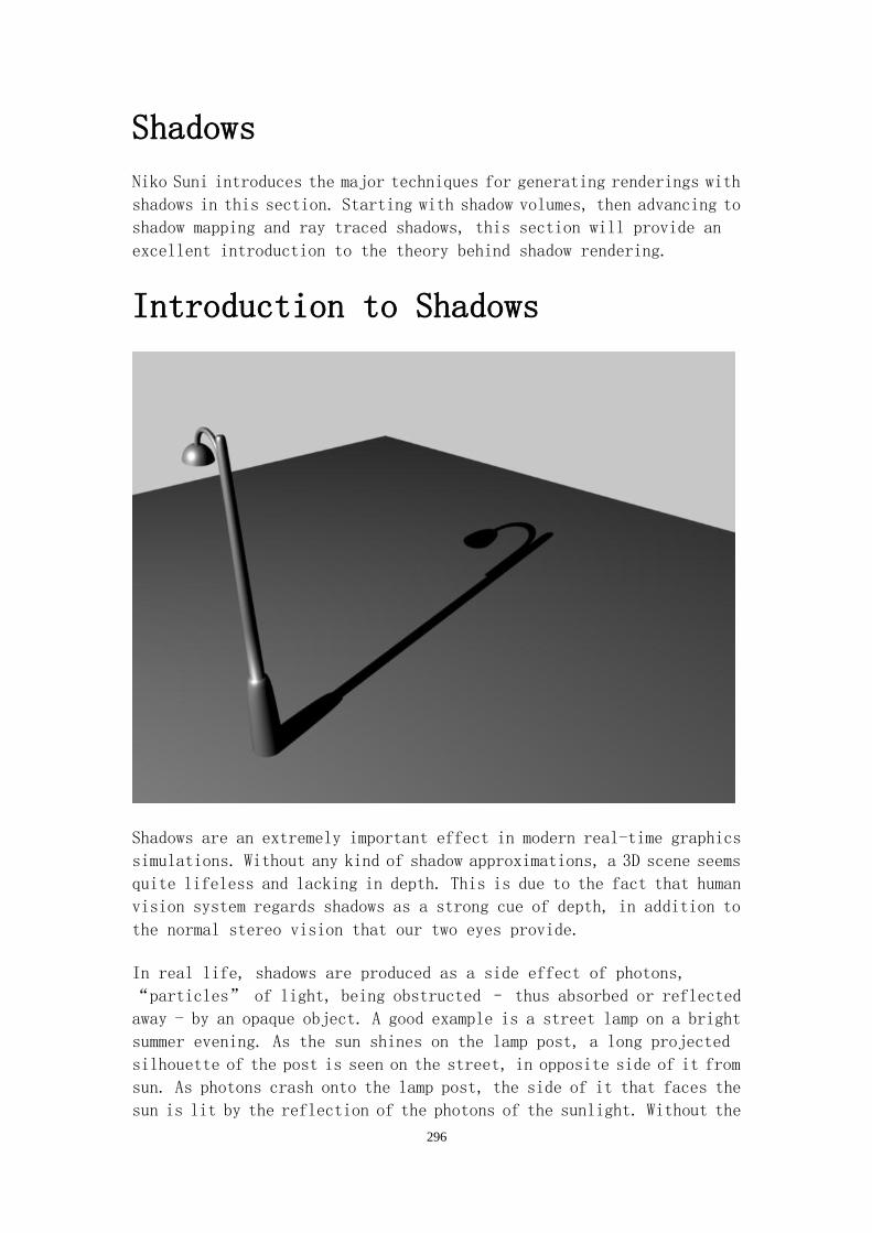
296

Shadows

Niko Suni introduces the major techniques for generating renderings with

shadows in this section. Starting with shadow volumes, then advancing to

shadow mapping and ray traced shadows, this section will provide an

excellent introduction to the theory behind shadow rendering.

Introduction to Shadows

Shadows are an extremely important effect in modern real-time graphics

simulations. Without any kind of shadow approximations, a 3D scene seems

quite lifeless and lacking in depth. This is due to the fact that human

vision system regards shadows as a strong cue of depth, in addition to

the normal stereo vision that our two eyes provide.

In real life, shadows are produced as a side effect of photons,

“particles” of light, being obstructed – thus absorbed or reflected

away - by an opaque object. A good example is a street lamp on a bright

summer evening. As the sun shines on the lamp post, a long projected

silhouette of the post is seen on the street, in opposite side of it from

sun. As photons crash onto the lamp post, the side of it that faces the

sun is lit by the reflection of the photons of the sunlight. Without the

297

lamp post, the said photons would go all the way to the pavement; with

the lamp post in the place, the photon flow is cut before the light reflects

off the street, thus depriving the street from light on the path of

obstruction.

An ideal simulation of the process that forms the shadow would be to trace

all the photons of the scene to all light receptors of the observer (or

in computer terms, pixels of the frame buffer), and performing

atomic-scale reflection and absorption calculations for each particle of

the scene while doing that. However, this poses a problem: modeling all

photon interactions with material particles, even in a simple scene, is

very expensive in computational terms; it would take infinite-like

amounts of memory just to store the photon starting points (or light

sources), not to mention each particle of the media that the said photons

are going to collide to. Add that to the fact that the mathematics for

quantum-scale particle interaction calculations aren’t exactly of the

light sort either. Multiply these astronomical figures with the fact that

you need to do the same process for each light sensor (or pixel) of the

observer, and you can figure that real shadows simply cannot be simulated

in purely physical manner, at least on existing computing architectures.

In real-time computer graphics, shadows have to be approximated as it is

not nearly feasible on current graphics technologies to simulate the real

photon flow with sufficient accuracy to fool the eye, while at the same

time run the simulation in frame rates sufficient to fool the brain to

see the movement of the scene and it’s object without noticing the

discrete frames of the simulation.

In the following shadow topics, we will take a look at two common

techniques used to approximate shadows in real time on Direct3D 10

hardware, a smaller look at ray-tracing approximation of shadows, and do

a comparison between these techniques and “real” behavior of shadows.

If you want to read more on approximation of the light reflection and

absorption – that is, what happens when the photons would reflect from the occluder - please refer to the chapter “Lighting models” in this

book.

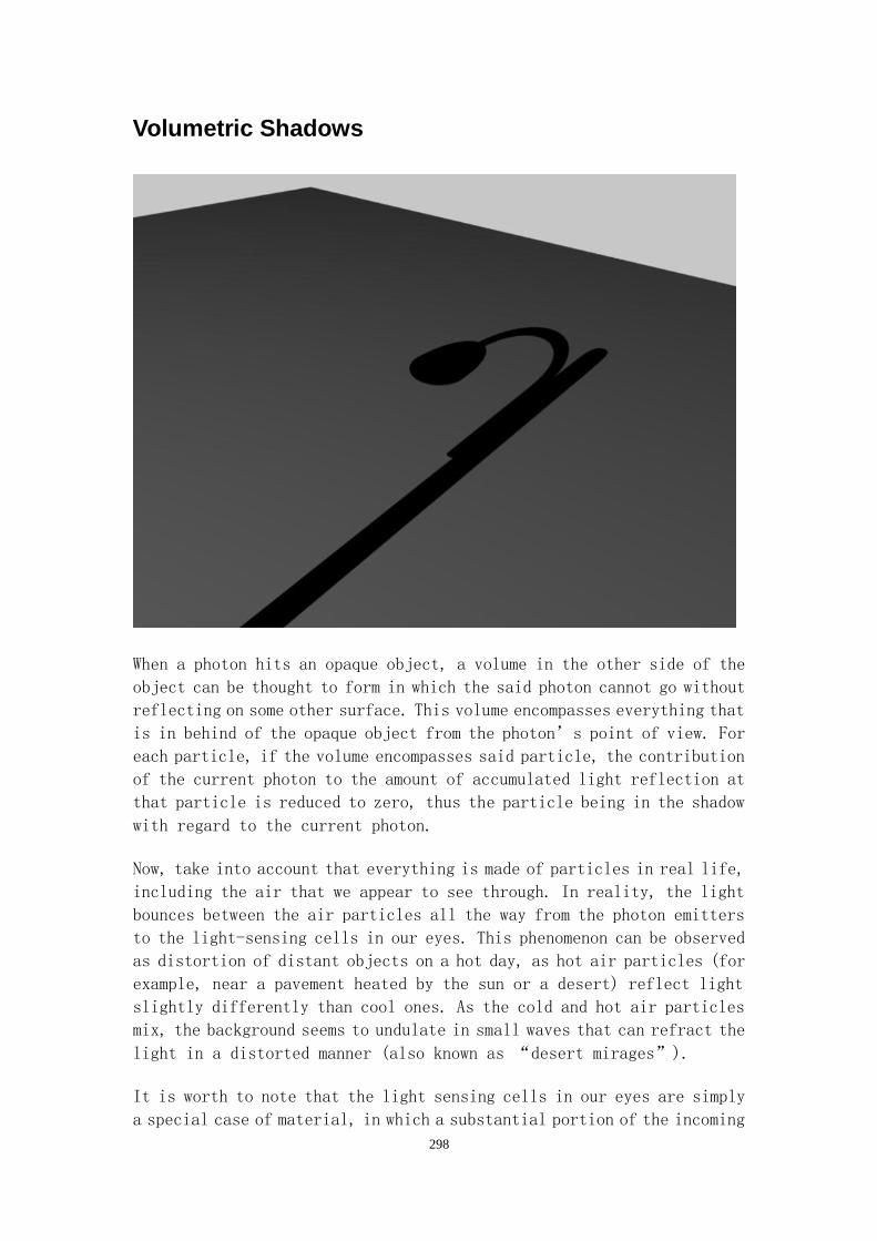
298

Volumetric Shadows

When a photon hits an opaque object, a volume in the other side of the

object can be thought to form in which the said photon cannot go without

reflecting on some other surface. This volume encompasses everything that

is in behind of the opaque object from the photon’s point of view. For

each particle, if the volume encompasses said particle, the contribution

of the current photon to the amount of accumulated light reflection at

that particle is reduced to zero, thus the particle being in the shadow

with regard to the current photon.

Now, take into account that everything is made of particles in real life,

including the air that we appear to see through. In reality, the light

bounces between the air particles all the way from the photon emitters

to the light-sensing cells in our eyes. This phenomenon can be observed

as distortion of distant objects on a hot day, as hot air particles (for

example, near a pavement heated by the sun or a desert) reflect light

slightly differently than cool ones. As the cold and hot air particles

mix, the background seems to undulate in small waves that can refract the

light in a distorted manner (also known as “desert mirages”).

It is worth to note that the light sensing cells in our eyes are simply

a special case of material, in which a substantial portion of the incoming

299

photons are converted to bio-electrical pulses for our brains to handle

as vision; for this reason, all of the steps for interacting with

“ordinary” material particles would also need to be repeated for each

of the receptor cell.

If you thought that all of the real process sounds very complex, you’re

quite right. As it is still not practical to simulate this behavior for

each discrete photon against each discrete material particle in the scene,

we make some broad approximations regarding the flow of the light in order

to establish our photon obstruction volumes for simulation:

- We will assume that the geometry which is to cast the shadows is uniformly

opaque; that is, every point of the shadow caster is equally blocking the

photons. We can simulate varying per-object opacity by varying the alpha

factor with which the shadow is finally blended in the scene.

-Conceptually, we regard the photon source as a single point or direction.

In reality, singular light sources do not exist in practice.

-A light is either occluded or reflected/absorbed by the occluding

geometry. This can be thought as using one large photon for the test

instead of trillions of them as in a real-life scene.

-We do not take into account that photons which would reflect off the

shadow caster could in fact end up to the shadow volume by means of another

reflecting material. This is a distinct possibility in reality, but human

eye cannot easily discern more than three orders of reflections, and only

a special scene (like a hall of mirrors) would make the phenomenon truly

stand out. Then again, a hall of mirrors is difficult to render with a

rasterizer anyway, because practically all material reflections depend

on each other.

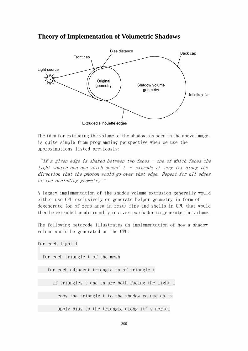
300

Theory of Implementation of Volumetric Shadows

The idea for extruding the volume of the shadow, as seen in the above image,

is quite simple from programming perspective when we use the

approximations listed previously:

“If a given edge is shared between two faces - one of which faces the light source and one which doesn’t – extrude it very far along the direction that the photon would go over that edge. Repeat for all edges

of the occluding geometry.”

A legacy implementation of the shadow volume extrusion generally would

either use CPU exclusively or generate helper geometry in form of

degenerate (or of zero area in rest) fins and shells in CPU that would

then be extruded conditionally in a vertex shader to generate the volume.

The following metacode illustrates an implementation of how a shadow

volume would be generated on the CPU:

for each light l

for each triangle t of the mesh

for each adjacent triangle tn of triangle t

if triangles t and tn are both facing the light l

copy the triangle t to the shadow volume as is

apply bias to the triangle along it’s normal

301

else

if triangles t and tn are facing in opposite

directions from the light l

take the edge e between triangles t and tn

copy the vertices of the edge e and move them by

the desired extrusion distance along the vector

from the light to the vertices

construct two triangles to form a quad between the

original edge vertices and the new vertices

apply bias to the quad along it’s normal

else

if triangles t and tn are both facing away from

the light l

copy the vertices of the triangle t to the shadow

volume and move them by the extrusion distance along

the vector from the light l to the vertices

apply bias to the triangle along it’s normal

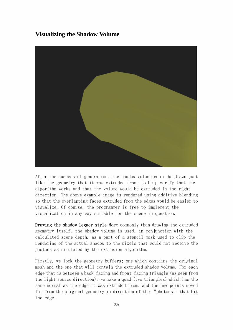
302

Visualizing the Shadow Volume

After the successful generation, the shadow volume could be drawn just

like the geometry that it was extruded from, to help verify that the

algorithm works and that the volume would be extruded in the right

direction. The above example image is rendered using additive blending

so that the overlapping faces extruded from the edges would be easier to

visualize. Of course, the programmer is free to implement the

visualization in any way suitable for the scene in question.

Drawing the shadow legacy style More commonly than drawing the extruded

geometry itself, the shadow volume is used, in conjunction with the

calculated scene depth, as a part of a stencil mask used to clip the

rendering of the actual shadow to the pixels that would not receive the

photons as simulated by the extrusion algorithm.

Firstly, we lock the geometry buffers; one which contains the original

mesh and the one that will contain the extruded shadow volume. For each

edge that is between a back-facing and front-facing triangle (as seen from

the light source direction), we make a quad (two triangles) which has the

same normal as the edge it was extruded from, and the new points moved

far from the original geometry in direction of the “photons” that hit

the edge.

303

A common practice in creating shadow volume is to generate “caps” to

the volume to limit it’s extents with regard to other geometry. For this,

we determine for each triangle if that triangle is facing the light or

not. If it is facing the light, we copy it to the shadow volume as is.

If it’s not, it is copied to the back side of the volume and translated

by the same vector used to extrude the edges. The caps of the volume are

useful to prevent the situation in which the observer is inside the shadow

volume and every other pixel except the ones at actually inside the shadow

volume are drawn shadowed, when using a method of shadow drawing called

“z-fail”.

At this step, we can move the resulting faces by applying a bias (a

correction vector) to the extruded quads along their normals so that the

shadow geometry doesn’t cause so-called “z-fighting”. Z-fighting is

a condition in which the shadow and the source geometry are in exactly

same screen-space depth and thus cause artifacts when rendered (as the

rasterizer has to “guess” which of them to draw on top of another). This

code shows how to apply a bias value to the triangles in order to eliminate

z artifacts, written in C++. Note that in practice the bias values are

best applied inside the extrusion loop:

VERTEX* allVertices; // VERTEX is defined as a structure with

a

// position vector. Actual definition of the type is omitted

here

// for brevity.

// the vertex buffer is assumed to be mapped/locked and the

data

// pointer copied to allVertices before this.

for (int i = 0; i < numTriangles; i++)

{

int vi0;

// Vertex index corresponding to the first vertex of

// the current triangle.

vi0 = i * 3;

// This works as each triangle has exactly three indices.

// The first vertex of the current triangle is at

// allVertices[i*3]. By applying specifying i*3+1 and i*3+2,

// we can address the other two vertices of the triangle.

D3DXVECTOR3 normal = D3DXVec3Normalize(...);

304

// Normal is calculated from the vertex positions; the actual

// calculation is omitted for brevity.

float bias = 0.001;

// The distance to move the triangles along their normals.

// The actual value is assumed to have initialized earlier.

// now we apply the bias to the original vertices:

for (int j = 0; j < 3; j++)

{

allVertices[vi0 + j] = allVertices[vi0 + j] - normal * bias;

//this does the actual moving of the vertices.

}

}

// Vertex buffer is unmapped/unlocked after the manipulation.

// This step is omitted for brevity.

Note that this implementation doesn’t even attempt to use special vertex

shaders for extrusion, so it could be use on any hardware that just

supports stencil buffers for the drawing step up next. There are methods

of using a vertex shader to do the extrusion step, but we will only cover

this basic approach and the one implemented with Direct3D 10 shaders for

simplicity. For the example implementations, I chose the z-fail method

for the stencil masking as it is an excellent algorithm for solid shadows

with no artifacts, in the situation where the observer is inside the shadow

volume. The z-fail algorithm is efficient in that it doesn’t need to

render a full-screen all-encompassing quad in order to visualize the areas

in the shadow volume – it simply doesn’t draw the scene in where the

stencil mask condition fails based on the volume.

Before the laying of the stencil buffer values takes place, we render an

ambient pass of the scene to establish a scene color for pixels that were

destined to be in the shadow, and the depth of the scene for the shadows

to clip to. Rendering ambient color will provide additional realism to

the scene as in real life, there are no perfectly shadowed objects. Some

light will always reflect from other light sources, and the ambient scene

pass would emulate this. The z-values are written so that the shadows will

clip to the rest of the scene correctly. The stencil buffer operations

should be disabled while rendering the ambient pass.

After preparing the shadow volume and drawing the ambient and z pass, we

set up some render states regarding depth and stencil buffer operations.

As we need to mask in the pixels that are in the shadow volume and on some

305

other geometry, we need to express a following sequence (assuming z-fail

render method):

1. Disable writing to depth buffer and color buffer. We don‟t need to see the actual volume

geometry, but we do need to manipulate the stencil buffer with it.

2. Set cull mode to “none”, so back-facing triangles are processed.

3. Depth compare function should be “less”, so that the shadow volume geometry behaves

like other objects in depth order but is drawn just slightly nearer to the observer than other

geometry (which normally uses “less or equal” function for depth comparison) to avoid

depth artifacts.

4. Two-sided stencil buffering should be enabled; otherwise, we would need separate passes

for incrementing and decrementing the stencil buffer values for front- and back-facing

volume geometry respectively.

5. Stencil reference value should be set to 1 to establish a default behavior for the mask, of

not rendering the shadow. Stencil mask and stencil write mask should have all bits up;

that is, have value 0xffffffff in order to use all stencil bits available if needed.

6. Both clockwise and counterclockwise stencil functions should be set to “always” to

denote that each and every pixel of the volume should contribute to the stencil buffer

values.

7. Counterclockwise stencil z fail function should be specified as “increase” and clockwise

“decrease” so as to properly increment and decrement the stencil values based on whether

the current pixel is front-facing or back-facing.

8. Stencil pass function for both clockwise and counterclockwise stencil operations should

be set to “keep” so that the stencil values would not get modified if the drawn pixels will

pass the depth test and therefore are of no interest of us.

This code listing, borrowed from the DirectX SDK February 2007 sample

“ShadowVolume10”, shows how to set the depth stencil state for two-sided

z-fail rendering:

DepthStencilState TwoSidedStencil

{

DepthEnable = true;

DepthWriteMask = ZERO;

DepthFunc = Less;

// Setup stencil states

StencilEnable = true;

StencilReadMask = 0xFFFFFFFF;

StencilWriteMask = 0xFFFFFFFF;

BackFaceStencilFunc = Always;

BackFaceStencilDepthFail = Incr;

BackFaceStencilPass = Keep;

BackFaceStencilFail = Keep;

306

FrontFaceStencilFunc = Always;

FrontFaceStencilDepthFail = Decr;

FrontFaceStencilPass = Keep;

FrontFaceStencilFail = Keep;

};

In addition to the above depth stencil state, the technique should also

set the culling rasterizer state to off in order to let the back-facing

triangles to affect the stencil and depth buffers, and blend state to “no

blending” so that unnecessary color writes are avoided.

After these steps, the extruded shadow volume can be rendered. For each

pixel, the above conditions are evaluated and the stencil buffer is

incremented and decremented if the conditions match the current pixel.

The rendering of the shadow volume establishes a stencil mask that can

be used to prevent the pixels from the actual scene to be rendered as

opposed to allowing shadow visualization color to be rendered

(essentially, z-fail as opposed to z-pass).

Moving on, we can now render the shadowed scene. As we need to render the

scene where the stencil value was left greater than 1, we need to establish

some stencil and depth rules again:

1. Z-buffering and stencil buffering should be enabled.

2. Z function should be reset to its default value of “less or equal” in order to render

normally.

3. If an ambient scene color was laid out before the stencil buffer manipulation step, we

need to enable alpha blending, set the blending operation to “add” and both source and

destination blend factors to “one” in order to additively blend the colors not in the

shadows with the ambient colors in the color buffer that lack the shadow information.

4. Stencil reference value should be 1 to establish the default mask value so that geometry

not in shadow will be rendered.

5. Stencil function should be set to “greater” to assure that correct pixels will be masked in.

6. Stencil pass behavior should be set to “keep” so that the stencil values don‟t get modified

in the next step.

Now, you can render the scene normally and those pixels that were in the

shadow as determined by the stencil mask – created by using the scene

depth and shadow volume information – are discarded based on the stencil

value.

The following code illustrates the most important steps to render

volumetric shadows using the z-fail technique.

307

//simple pixel shader that returns a constant ambient color.

// it is assumed that a PSSceneIn structure contains the

// output of the ordinary vertex shader – position and normal.

float4 PSAmbient(PSSceneIn input) : SV_Target

{

return g_vAmbient; //global ambient color variable

}

//pixel shader for diffuse color:

float4 PSDiffuse(PSSceneIn input) : SV_Target

{

return input.color; //just pass on the diffuse color from

vs

}

//pixel shader for shadow rendering:

float4 PSShadow(PSShadowIn input)

{

//PSShadowIn contains only the position from the shadow

//vertex shader.

return float4( 0.0f, 0.0f, 0.0f, 0.5f ); //black shadow

}

//VSShadow omitted – outputs vertices in world space to gs

//VSScene omitted – calculates diffuse color of the scene and

// outputs vertices in projection space

// GSShadow geometry shader is discussed later.

//The following techniques then utilize the above

functionality:

//renders the scene diffuse colors:

technique10 RenderDiff

{

pass p0

{

SetVertexShader( CompileShader( vs_4_0, VSScene

() ) );


SetPixelShader( CompileShader( ps_4_0, PSScene () ) );

//since the diffuse pass occurs after the ambient color has

308

//been already laid out, we need to blend it additively:

SetBlendState( AdditiveBlending, float4( 0.0f, 0.0f,

0.0f, 0.0f ), 0xFFFFFFFF );

//reset the depth stencil state to ordinary rendering:

SetDepthStencilState( RenderNonShadows, 0 );

//and enable back-face culling:


}

}

// this technique calls the shadow volume extrusion and

// manipulates the stencil buffer:

technique10 RenderShadow

{

pass p0

{

SetVertexShader( CompileShader( vs_4_0, VSShadow() ) );

SetGeometryShader( CompileShader( gs_4_0,

GSShadow() ) );

SetPixelShader( CompileShader( ps_4_0, PSShadow() ) );

//we don’t want to write colors here:

SetBlendState( DisableFrameBuffer,

float4( 0.0f, 0.0f, 0.0f,0.0f ), 0xFFFFFFFF );

SetDepthStencilState( TwoSidedStencil, 1 );

SetRasterizerState( DisableCulling );

}

}

//this simple technique just lays out the ambient color of

the scene:

technique10 RenderAmbient

{

pass p0

{

SetVertexShader( CompileShader( vs_4_0, VSScene() ) );


SetPixelShader( CompileShader( ps_4_0, PSAmbient() ) );

SetBlendState( NoBlending,

float4( 0.0f, 0.0f, 0.0f, 0.0f ), 0xFFFFFFFF );

SetDepthStencilState( EnableDepth, 0 );


}

309

}

// These techniques are used in the host application as

follows:

// 1: render ambient

// 2: render shadow

// 3: render diffuse, which is now clipped by the shadow

stencil.

It is possible to render volumes of multiple lights at the same time, and

the z-fail algorithm still works as intended.

The volumetric shadow technique in general produce very sharp shadows,

but it is possible to integrate over a number of lights to simulate an

area light that creates smooth shadow edges. This will require additional

passes for the drawing of the shadowed scene, though, and CPU needs to

be utilized between the passes to control the parameters of the passes.

In the DirectX SDK, a method of using a vertex shader to do the extrusion

is presented to alleviate this cost, but it still requires the CPU to

initiate and feed each pass with their parameters.

Bottlenecks in the legacy approach The volumetric shadowing technique,

as described previously, has a couple of bottlenecks that are evident when

implementing it in hardware earlier than Direct3D 10 generation. These

mainly have to do with unnecessary CPU utilization and graphics bus

bandwidth saturation.

Firstly, it takes considerable time from the CPU to perform the volume

extrusion as opposed to having the graphics card do it. The graphics

processing unit is optimized for parallel vector calculations (of which

the extrusion operation is full). Compare it to the central processing

unit which, while very flexible with regard to the nature of the

calculations, only allows a small amount of parallel vector operations

per instruction and therefore is inefficient in most 3d graphics

calculations.

The CPU load can be eased by doing the extrusion in the vertex shader,

but then another problem surfaces: a heavy amount of extra geometry, in

the form of degenerate triangles for each edge and open vertex must be

calculated and baked into the geometry buffers, which in turn takes a lot

of extra memory and graphics bus bandwidth.

In cases with large amounts of graphics primitives, this also causes the

geometry processing pipeline to choke because the extrusion vertex shader

310

is run for each vertex regardless of whether it is going to be extruded

or not, and this load is multiplied with the number of extra vertices that

make possible to use vertex shader for the operation to begin with.

Direct3D 10 allows us to do the extrusion step entirely in the graphics

processor, without CPU intervention, thus effectively eliminating both

of these bottlenecks in one sweep. This, combined with the immense

geometry processing power available on Direct3D 10 cards due to the

unified shader pipelines, allows for large performance boosts over the

legacy technique presented earlier.

Using Geometry Shader to Implement Volumetric Shadow

Extrusion

311

To extrude the shadow geometry in Direct3D 10, we can use the new component

of the graphics pipeline, the geometry shader. A geometry shader works

one graphics primitive (like triangle, line or point) at a time, and can

access adjacency information of the current primitive so as to determine

whether the current triangle’s edge is a candidate for the extrusion

along the light’s path.

In addition to the positions, normals and other data associated with the

vertices of the geometry to be extruded by the geometry shader, we need

to pass the adjacency data to the pipeline in the form of extra index data

for each triangle, interleaved with the original indices of the geometry.

The vertex data input parameter to the geometry shader is represented as

an array of vertex structures, with 6 as the number of elements to consider

the adjacent vertices of the triangle in addition to the triangle itself.

Firstly, the geometry shader determines if the current triangle is facing

the light source. If it isn’t, there’s no need to perform the rest of

the shader as the current triangle wouldn’t be affected by light anyway,

and thus the geometry shader can fall through with no output corresponding

to the current triangle. If the triangle did face the light source, then

we’d perform a few steps more in the geometry shader. For each edge of

the triangle, it is determined whether that particular edge is on the

silhouette of the geometry with regard to the light position. If it is,

new triangles are created inside the geometry shader to construct the

extrusion faces for that edge.

After the edges have been extruded, the current triangle is capped from

both the front and back side to construct a solid volume out of it, in

a similar fashion as the legacy approach does. As was discussed before,

this prevents the volume from “leaking” when the observer is inside it

during the shadow visualization phase.

The generated primitives are output from the geometry shader to a

TriangleStream object which has a template type corresponding to the input

to the pixel shader. The TriangleStream has two methods; Append() adds

one vertex to the output, and RestartStrip() terminates the current

triangle strip being output and begins a new one. New vertices calculated

in the geometry shader are appended to the output stream and between each

edge qualifying for the extrusion, the start cap and the end cap, a new

triangle strip is started to distinguish the different parts of the output

for the rasterizing steps after the geometry shader. The bias value is

applied to the new geometry in the geometry shader, for the same reason

as in the legacy implementation.

312

//The following geometry shader code is borrowed from the

DirectX SDK samples:

//

// Helper to detect a silhouette edge and extrude a volume

from it

//

void DetectAndProcessSilhouette( float3 N,

// Un-normalized triangle normal

GSShadowIn v1,

// Shared vertex

GSShadowIn v2,

// Shared vertex

GSShadowIn vAdj,

// Adjacent triangle vertex

inout TriangleStream<PSShadowIn> ShadowTriangleStream

// triangle stream

)

{

float3 NAdj = cross( v2.pos - vAdj.pos, v1.pos - vAdj.pos );

float3 outpos[4];

float3 extrude1 = normalize(v1.pos - g_vLightPos);

float3 extrude2 = normalize(v2.pos - g_vLightPos);

outpos[0] = v1.pos + g_fExtrudeBias*extrude1;

outpos[1] = v1.pos + g_fExtrudeAmt*extrude1;

outpos[2] = v2.pos + g_fExtrudeBias*extrude2;

outpos[3] = v2.pos + g_fExtrudeAmt*extrude2;

// Extrude silhouette to create two new triangles

PSShadowIn Out;

for(int v=0; v<4; v++)

{

Out.pos = mul( float4(outpos[v],1), g_mViewProj );

ShadowTriangleStream.Append( Out );

}

ShadowTriangleStream.RestartStrip();

}

//This is the crux of the code. It calls the above function

as

313

//needed, and generates the cap geometry for the shadow

volume.

//

// GS for generating shadow volumes

//


void GSShadowmain( triangleadj GSShadowIn In[6], inout

TriangleStream<PSShadowIn> ShadowTriangleStream )

{

// Compute un-normalized triangle normal

float3 N = cross( In[2].pos - In[0].pos, In[4].pos -

In[0].pos );

// Compute direction from this triangle to the light

float3 lightDir = g_vLightPos - In[0].pos;

//if we're facing the light

if( dot(N, lightDir) > 0.0f )

{

// For each edge of the triangle, determine if it is

a silhouette edge

DetectAndProcessSilhouette( lightDir, In[0], In[2],

In[1], ShadowTriangleStream );





//near cap

PSShadowIn Out;

for(int v=0; v<6; v+=2)

{

float3 extrude = normalize(In[v].pos -

g_vLightPos);

float3 pos = In[v].pos + g_fExtrudeBias*extrude;

Out.pos = mul( float4(pos,1), g_mViewProj );


}


//far cap (reverse the order)

for(int v=4; v>=0; v-=2)

314

{

float3 extrude = normalize(In[v].pos -

g_vLightPos);

float3 pos = In[v].pos + g_fExtrudeAmt*extrude;

Out.pos = mul( float4(pos,1), g_mViewProj );


}


}

}

Apart from the extrusion step discussed herein, the application of the

extruded data to create the stencil values is the same on both the old

and the new way. However, doing the extrusion in the geometry shader saves

some valuable clock cycles in both the CPU and GPU as compared to using

vertex shaders with extra geometry. It is clear that programmers using

Direct3D 10 should embrace the new method for increased geometry

performance with virtually no handicaps as compared to the legacy way.

It should be noted that the volumetric shadow technique itself has a flaw

that is not trivial to fix: as the regular lighting of the scene regularly

uses normals interpolated between the vertices, the shadow volume

extrusion is based on the normals of the faces at the silhouette edge of

the geometry. This means that the extruded edges of the shadow volume

overlap the regular shading in parts where the triangles of the edge would

be lit by the interpolated light values. The overlap is best described

as an irregular sawtooth edge artifact along the triangles connected to

the silhouette edges from the lit side of the geometry, as seen in the

following image (with the artifact boundary marked with red line):

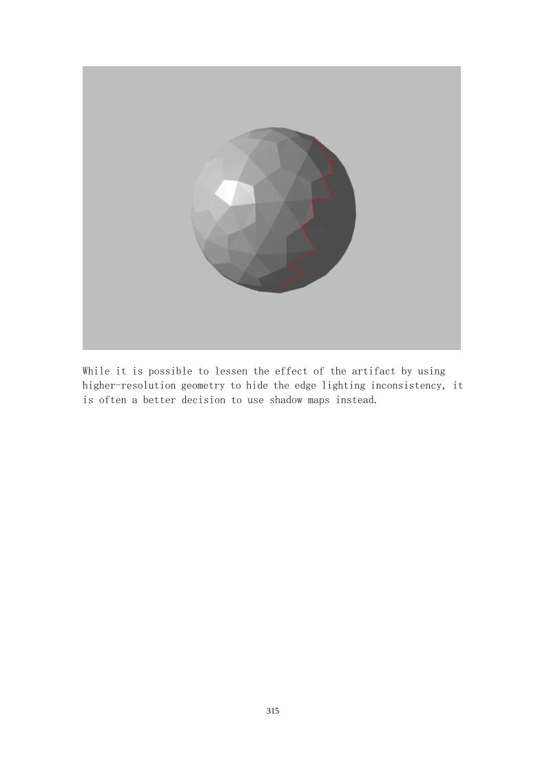
315

While it is possible to lessen the effect of the artifact by using

higher-resolution geometry to hide the edge lighting inconsistency, it

is often a better decision to use shadow maps instead.

316

Shadow Mapping

An another approach to shadowing, bitmapped shadow (or shadow map)

techniques attempt to emulate the light occlusion by using a discrete grid

of “photons”, in the form of texels of a depth texture that is projected

from the light source to the occlusion geometry and to the scene. This

is in contrast to the volumetric shadow technique which explicitly

processes the geometry of the shadow casters, in that bitmapped shadow

techniques are very much independent from the geometric complexity of the

said shadow casters.

As compared to volumetric shadows, they can consume far less gpu resources

as it isn’t nearly always needed to match the shadow map resolution to

the full viewport resolution, thus saving fill rate and memory bandwidth

at the cost of the video memory for the shadow maps themselves. Shadow

maps will also work more readily with various types of filtering, because

as at heart they are textures, shadow data adjacent to currently evaluated

"photon" is always available.

Theory of depth map shadows

Bitmapped shadows generally work by first projecting the depth of the

scene to a texture from the light source’s perspective. Then, during the

317

main rasterization of the scene, the texture is projected from the lamp

space to the camera space and its depth value is compared to the current

pixel’s depth value.

The following image illustrates the depth of the scene – on the left,

from camera space and on right, from the light’s space:

The scene needs to be projected into the same space in which the light

source’s depth texture was rendered in order for the depth values to be

comparable. This can be accomplished by transforming the scene’s

geometry into the light space in a special vertex shader that, in addition

to the normal duties of a vertex shader, calculates the light-space

position of each vertex and outputs it into the pixel shader for the shadow

testing phase.

The shadow test, in its most basic form, draws the scene as follows: The

shadow depth texture rendered earlier is projected to the scene. Then,

the scene is drawn in an ordinary manner. During this drawing, a pixel

shader does the depth check: if the current pixel’s depth in the light

space is greater than the shadow depth map’s projected depth value, the

current pixel is in shadow as it is behind the shadow caster. This

knowledge can be used to modulate the color of the pixel being drawn, so

as to simulate the occlusion of the photons from the light source. As the

depth values are compared, a depth bias value can be used to reduce the

artifacts that result from the inevitable inaccuracy in depth buffer

values. Without it, the shadows could reach to faces that they don’t

belong to, or the shadows might not show on surfaces that are supposed

to be shadowed.

A filter can be applied to the depth testing procedure to smooth the

transition from shadowed to non-shadowed pixels and reduce the staircase

effect that is inherent in bitmap-based techniques. Another way of

increasing the fidelity of bitmapped shadows is to simply make the texture

rendered from the light space depth larger in dimensions.

318

In the following image, the shadow on the left is rendered without

filtering, and the one on the right using 4-tap percentage-close filtering:

This code listing shows how to render the scene depth from the light’s

perspective:

cbuffer cb1

{

//ordinary wvp transformation:

matrix worldViewProj;

//light-space equivalent:

matrix lightWVP;

//other buffer members omitted for clarity.

}

//shadow pixel shader input structure:

struct SHADOWPS_INPUT

{

float4 Pos : SV_POSITION; //ordinary position

float3 Pos2D : TEXCOORD0; //Unclamped position

};

// Bitmapped shadow vertex shader.

SHADOWPS_INPUT ShadowVS( VS_INPUT input )

{

SHADOWPS_INPUT output = (SHADOWPS_INPUT)0;

//Here, we apply a geometric bias so as

// to reduce self-shadowing:

input.Pos += input.Norm * 0.1;

output.Pos = mul( float4(input.Pos*100,1), ShadowWVP);

319

//In order to preserve the full range of coordinates,

// we copy the position to a texture coordinate too.

output.Pos2D = output.Pos.xyz;

//we don't need other components at the shadow drawing.

// Depth is relayed to the pixel shader already.

return output;

}

//a pixel shader for the bitmap shadow generation.

float4 ShadowPS( SHADOWPS_INPUT input) : SV_Target

{

float4 cDiffuse = (float4)0;

cDiffuse.rgba = input.Pos2D.z / maxDepth;

return cDiffuse;

}

Here’s how to test the projected scene depth against the results of the

shadow rendering:

struct VS_INPUT

{

float3 Pos : POSITION;

float3 Norm : NORMAL;

float2 Tex : TEXCOORD0;

};

struct ORDPS_INPUT

{

float4 Pos : SV_POSITION; //ordinary position

float4 ShadowSamplePos : TEXCOORD0; //light-space position

float3 Norm : TEXCOORD1; // Normal for per-pixel light calculation

float RealDist : TEXCOORD2; //Real distance from the eye to the scene

float3 Pos3D : TEXCOORD3; //Position in object space

};

// This is the depth map shadow test vertex shader.

// In addition to usual vertex shader tasks, it

// outputs a light-space position too so that the

// pixel shader can compare the scene's depth values

// with the previously rendered depth map.

ORDPS_INPUT VS( VS_INPUT input )

320

{

ORDPS_INPUT output = (ORDPS_INPUT)0;

output.Pos = mul( float4(input.Pos*100,1), World);

output.Pos = mul( output.Pos, View);

output.Pos = mul( output.Pos, Projection);

//We calculate the shadow-space vertex position by

//transforming the input with the shadow matrix.

output.ShadowSamplePos = mul( float4(input.Pos*100,1),

ShadowWVP);

//we need to accommodate the max depth here if we

//are using fixed function depth maps.

output.RealDist = output.ShadowSamplePos.z / maxDepth;

output.Pos3D = input.Pos;

output.Norm = mul( input.Norm, (float3x3)World );

return output;

}

// This is the depth test pixel shader. It determines

// whether the current pixel is in shadow or not,

// and outputs color accordingly.

float4 PS( ORDPS_INPUT input) : SV_Target

{

// Calculate lighting assuming light color is <1,1,1,1>

float fLighting = saturate( dot( input.Norm, vLightDir ) );

float4 cDiffuse = (float4)fLighting;

cDiffuse.a = 1;

//We'll continue a little bit with the shadow mapping.

float2 projTexCoord;

//Project the shadow-space position to screen xy by dividing the values

with w.

projTexCoord.x = input.ShadowSamplePos.x / input.ShadowSamplePos.w;

projTexCoord.y = -input.ShadowSamplePos.y / input.ShadowSamplePos.w;

//Then bias the coordinates to texture space so that the projected range

transforms from -1...1 to 0...1.

321

projTexCoord += 1.0f;

projTexCoord *= 0.5f;

//Sample the shadow-space depth from the scene rendered

// in shadow space:

float currentDepth = g_txShadowDepth.Sample(samLinearClamp,

projTexCoord);

//We apply a little bias to the depth values so that our geometry

// doesn't, for the most part, shadow itself.

if (!((input.RealDist -1.0f/20.0f) <= currentDepth))

{

cDiffuse.rgb *= 0.2f;

}

// NOTE: The texture object also has a method "SampleCmp" which

// can take in a comparison operation,

// perform depth comparing given reference and return a value

// between 0 and 1 depending on the portion of the four PCF

// (percentage closer filtering) sub-samples that pass the

// comparison.

// SampleCmp uses hardware coverage filtering so it results in

// better quality shadow edges with essentially no extra fillrate

// cost.

// Please check the recent DirectX SDK documentation for up-to-

// date info about this feature.

// The SampleCmp method is very sensitive wrt. the format of the

// depth buffer (internal format must be untyped) and the

// the choice of view formats is very restricted.

return cDiffuse;

}

Cubic shadow maps

As the depth from the light is projected with a perspective matrix, it

is unsuitable for point light sources that cast light and shadows in all

directions; instead, it is best used with a spotlight or a directional

322

light source as the direction of the light (and therefore of the shadow)

from the source is somewhat uniform and possible to accurately map to a

2D texture.

Fortunately, we can simulate shadows from a point light by using 6

different spotlight-like shadow buffers for the light, arranged in a cube

fashion around the light source.

Direct3D 8 and 9 provide cube maps, a special type of texture with 6

separate faces for up, down, back, forward, left and right directions for

this kind of purposes. However, with Direct3D 8 and 9, each face of the

cube has to be rendered separately, each with own matrices and draw calls.

As draw calls and state changes cause bottlenecks in the Direct3D system

due to the physical time it takes to make those calls as well as causing

the graphics system to stall due to over-serialization of the commands,

it is beneficial if we can minimize the number of these calls when

rendering anything.

Efficient drawing of cubic shadow maps in Direct3D 10

Direct3D 10 introduces the concept of resource views; that is, video

memory can be mapped to almost arbitrary representation. In the case of

a cube map, the data for the cube faces can be represented to the shaders

as an array of 2D textures and be indexed in that fashion in the geometry

shader, to be used again in a cube map form for depth testing against the

scene after the rendering of the depth values from the light’s point of

view.

In the geometry shader, we can direct our primitives to a given render

target by using an integer component having the system-defined semantic

SV_RenderTargetArrayIndex on our output vertex structure. As we process

each triangle, we copy it to all the render targets in the array by

iterating through the render targets array and using the index of each

render target to fetch the correct transformation matrix - for each given

render target direction as mapped to a cube – from the effect parameters.

The following example code shows how to create a view for a 6-face render

target array:

D3D10_RENDER_TARGET_VIEW_DESC DescRT;

DescRT.Format = cubeDepthTexture.Format;





323

pd3dDevice->CreateRenderTargetView( cubeDepthRes, &DescRT,

&pCubeDepthRTV);

We can then use the rendered cube texture in the shadow comparison function

by projecting it to the scene, much like how we processed the single

spotlight shadow.

There are some things to keep in mind though: As of Direct3D 10, you can

only set one depth stencil surface to the device at any given time. This

means that you need to store the depth values in the color data of the

render targets. Fortunately, D3D10 pixel shaders let us to handle

arbitrary values (including colors) as depth via views to typeless

resources, so this isn’t a problem.

Here’s a basic geometry shader which uses the render target index

semantic to direct output:


void GS_CubeMap( triangle GS_CUBEMAP_IN input[3], inout

TriangleStream<PS_CUBEMAP_IN> CubeMapStream )

{

//iterate all 6 directions of the cube map:

for( int f = 0; f < 6; ++f )

{


PS_CUBEMAP_IN output;

//output.RTIndex is an integer declared with the

//render target index semantic.

output.RTIndex = f;

//output a whole triangle for each cube face. The rasterizer

//will determine if they actually get drawn or not:

for( int v = 0; v < 3; v++ )

{

//lightViewMtxs is an array of matrices that determine the light

//positions and orientations for each of the main directions:

output.Pos = mul( input[v].Pos, lightViewMtxs[f] );

//mProj is a projection matrix that contains a 90-degree

//perspective. 90 * 4 = 360 degrees so all directions around

//the cube are considered.

output.Pos = mul( output.Pos, mProj );



}


324

}

}

Note that you need to declare a pixel shader input with the render target

index semantic too, so that the index goes all the way to the rasterizer.

The rest of the shadow map rendering procedure is the same as in

single-target shadow map rendering. In the depth compare pixel shader,

you need to loop thru all the faces of the cube map and handle the texture

colors as depths, but otherwise this part is exactly the same as in the

single shadow map technique too. This image shows a simple test scene for

the technique:

Ray-traced shadows

325

The pixel processing power of the modern graphics processors is beginning

to enable real-time ray-tracing applications, even though the fill rate

limits and relatively rigid data structure requirements of even the

top-of-the-line graphics processors dictate that full ray-tracing isn’t

a viable option for entire scenes designed for real-world usage just yet.

Ray-tracing is a method of brute force light evaluation, in which for each

pixel in the frame buffer, a ray is collided with the scene objects to

determine the reflected color of the object. The ray can be traced further

than the first collision with the scene, to produce effects like mirror

or glass.

Ray-traced shadows are evaluated in a similar way, but instead of

evaluating the collision of rays from the frame buffer to the scene, the

collision check is performed on rays from the scene to the light source.

Should the ray from the current pixel collide with some object before

reaching the light source, the current pixel would be in shadow and thus

its color could be modulated darker from its basic material color. A severe

limitation for using ray-tracing in Direct3D 10 is that you can’t

evaluate arbitrary mesh data in the context of a pixel shader due to

inherent rasterizer-oriented architecture. However, if you can model your

shadow casting geometry mathematically (using relatively optimized

formulas for performance), you can evaluate the collision steps

326

relatively easily for each rendered pixel and get fantastic-looking

results.

An intriguing aspect of using per-pixel ray-traced shadows is that by

virtue of evaluating each and every result pixel independently, the shadow

need not be uniform of nature. Consider a solid glass ball, for example;

the simulated photons (rays) refract with more intensity when traced near

through the center of the ball rather than near the edge of the same ball

due to Fresnel refraction coefficient. The rays could even be bent by the

ball to create a caustic distribution of the shadow and the light that

would actually amplify the light in some points of the shadow receiver

instead of making them appear like in shadow.

Following is a small code sample which implements a ray-traced shadow

evaluator in pixel shader. The occluding geometry is a simple ball, but

any object that can be expressed as a mathematical formula in pixel

shader’s terms could be used.

//this function returns the distance of a point to a line:

float dist_p2l(float3 pnt, float3 l0, float3 l1)

{

float3 v = l1 - l0;

float3 w = pnt - l0;

//determine the relations of the dot products of a triangle

//formed by the vectors

float c1 = dot(w,v);

float c2 = dot(v,v);

float b = c1/c2;

//and use them to calculate the distance.

float3 pb = l0 + b * v;

return distance (pnt, pb);

}

float getSphereIntersect(float3 lightPos, float3 pixelPos,

float3 ballPos, float ballRadius, out bool hit)

{

hit = true;

float dist = dist_p2l(ballPos, pixelPos, lightPos);

if (dist > ballRadius) {hit=false; return 0;}

else

//prepare the shadow intensity here.

327

return 1-cos(1.0-(dist/ballRadius));

}

//this is the ray tracing shadow pixel shader.

//it uses the above function to determine the shadow

intensity.

float4 RaytraceShadowPS(PS_In input) : SV_Target

{

bool hit;

float shadowIntensity;

shadowIntensity = getSphereIntersect(g_lightPos,

input.wsPosition, g_ballPos, g_ballRadius, hit);

float4 ret = input.color;

if (hit)

ret.rgb *= shadowIntensity;

return ret;

}

Direct3D 10.1 considerations for shadow rendering

Direct3D 10.1, a new version of the Microsoft’s graphic API announced

in late 2007 and launched at March 2008, provides two new capabilities

that are very suitable for rendering shadows more efficiently than with

the 10.0 baseline:

Gather instruction

This new texture-related instruction can be used to load the red

components of 4 nearest texels of a texture to a float4 register, given

a sample position. While the classic-style texture sampler is sufficient

for most texturing purposes with point, bilinear and trilinear filtering

capabilities, using the Gather instruction enables the developer to

access the raw data of the sample and implement a custom filtering

algorithm for quality enhancement or special effects.

As Gather only loads the red components of the source texels, it is not

directly usable to replace the default samplers when dealing with ordinary

color data – instead, the method is most useful in implementing a custom

filter for shadow map edges. If the developer has an error heuristic

328

available at the time of drawing a shadow map, that heuristic can be used

in weighting the 4 samples together for far higher quality than the default

4-tap filter is capable of. The error heuristic could be as simple as a

texture of 2D vectors telling how far the actual edge of the shadow caster

is at any given shadow texel. Also, sophisticated image-space shadow edge

blurs become more feasible.

Gather is represented by a method in the texture object, when the HLSL

code is compiled with the 4.1 profile. The source texture must contain

a red channel; for typeless depth textures, this typically matches the

first and only channel that, unsurprisingly, represents depth values.

Cube map arrays

Direct3D 10.1 introduces the ability to address multiple cube maps as

shader-indexable arrays. For shadows, this means that it is possible to

simultaneously create cubic shadow maps for arbitrary number of point

lights by using single draw call; this contrasts the way that baseline

10.0 needs all the cubes to be rendered with their own draw calls. When

using the generated shadow cubes to render the shadowed scene, the pixel

shader can again access them as source array of cubes for further

efficiency gains.

To create cube map arrays, create a resource of type Texture2DArray

containing enough data to fill your cube array. Then, create a shader

resource view for this resource by using the new method

ID3D10Device1::CreateShaderResourceView1() that is a new version of this

method for the Direct3D 10.1 functionality level devices. The

D3D10_SHADER_RESOURCE_VIEW_DESC1 structure used in that method has been

augmented from the 10.0 baseline version in that it can contain a new

resource view parameter structure, D3D10_TEXCUBE_ARRAY_SRV1. In addition

to the ordinary cube map parameters, this structure has an integer member

“NumCubes” that you can use to specify the number of distinct cubes for

your resource view. Bound as a render target, a cube map array is indexed

in the same fashion as an array of 2D textures; there is no separate render

target view exclusively for cubes.

When using texture cube arrays as input to the pixel shader, use the new

type TextureCubeArray to declare the reference to your cube array resource

view; as you then sample the data from the array, use the first three

texture coordinate components as the normal that you would use with

sampling a single cube, and set the w component to the index of the cube

that you want to use.

329

Level Of Detail Techniques

In this section, Niko Suni investigates several aspects of how level of

detail can be implemented. Concepts for managing scene level of detail

are presented, followed by per-object level of detail with tesellation

techniques.

Managing Level Of Detail

Level of detail control is generally practiced in order to spare computing

resources and time in rendering entities of a graphics model. For example,

if a game character is a very far from the player’s viewport (thus appears

small on the screen), it is not beneficial to use very complex shaders

or geometry to render that character. Fancy effects and sharp details

wouldn’t be very visible from the distance.

We’d need to render something to depict the character. The player would

definitely notice the sudden appearance of the character if he/she

approached the entity. If the character would actually be of size less

than one pixel, we could just not render it and the player wouldn’t notice

a thing.

330

A level of detail control flow usually involves removing detail from a

renderable entity. This is accomplished either by removing geometric

primitives, reducing the precision of the elements that the entity

comprises of or using smaller textures and/or simpler shaders to render

said entity.

In older graphics architectures, the geometry-related level of detail

adjustments almost always required CPU intervention, thus incurring extra

overhead to the operation that is supposed to reduce the system load.

The generalized shader pipeline architecture of Direct3D 10 enables us

to conditionally draw and remove geometry in both object and primitive

level, compress the data and dynamically control shader flow to achieve

all the methods of controlling level of detail in hardware, without direct

involvement of the CPU (except for initial programming of the graphics

processor). Next, we look at these methods in detail, starting from the

object-level culling and finishing to the conditional flow implemented

in pixel shaders.

Occlusion Culling Basics

Occlusion culling is a popular technique for reducing the drawing workload

of complex 3D scenes. In legacy implementations, it works basically as

follows:

1. Using standard drawing techniques, render the potentially occluding objects in the scene

with depth writing enabled as usual.

2. For each object that is potentially occluded, start a query which counts how many pixels

pass a depth buffer test. This is generally called initiating an “occlusion query”, because

with it we can determine if subsequent geometry drawn is occluded based on earlier depth

values of the scene.

3. Draw the current object‟s bounding geometry to the scene. We can disable drawing of the

object to depth, color or stencil buffers, as the point of this step is that the current

occlusion query keeps record of how many pixels of the said geometry did pass the depth

buffer test against the scene depth established in the step one.

4. End the current occlusion query and try to download from the graphics processor the

amount of pixels that passed the depth test in the previous step.

5. If the number of pixels that passed the depth test in step 3 was greater than zero, there is a

very likely possibility that the object was not entirely occluded by the objects rendered in

step 1. Therefore we should render the current object normally to the scene.

331

On the other hand, if the number of the pixels that passed the depth test

was zero, the object’s bounding geometry (and therefore the actual object)

was definitely fully behind the geometry rendered in step 1. Therefore,

we can ignore the drawing of the current object and move on to draw other

objects as applicable.

Upon trying to download the occlusion data, the graphics card may report

that the data isn’t available yet. In this case, we have to either wait

for the data to become available or just proceed with rendering the

detailed object.

There is a delicate balance of performance between giving up the query

and just rendering the object, or being optimistic and waiting that the

query, when it does successfully return the data, confirms that we don’t

need to render the object. For small to moderate amounts of primitives

in the detail geometry, it is statistically not worth the wait the results

beyond one occlusion data download attempt; instead, it is preferable to

just render the said detail geometry because drawing it would take less

time than the wait for the data combined with the time it takes to actually

call the download. Of course, the balance depends on the combination of

the scene, the graphics hardware performance and the performance of the

rest of the system including the CPU.

Shortcomings of the legacy implementation

Before Direct3D 10, occlusion culling was quite bothersome to set up and

manage, and despite some potentially significant savings in rasterizer

utilization, more often than not the overhead of actually doing the

occlusion culling routine outweighed the benefits towards overall

application performance improvement.

It takes a certain time to route a graphics call all the way from the

application to the graphics processing unit. This time varies between

specific calls, but is significant as compared to the time it takes to

perform simple to middle complexity calculations locally in either the

CPU or GPU. This delay is due to many reasons, but the primary reason is

the transition of the call from application layer to kernel layer in the

operating system and the CPU.

Another significant delay can be caused by the latency and bandwidth of

the graphics bus, but this ceases to be a very large bottleneck today due

to massive bus bandwidths offered by the modern system board designs and

memory electronics performance. Yet another potential delay is caused by

the fact that if data required to fulfill a given graphics call isn’t

332

ready by the time of the said call’s execution, the system will have to

wait until the data does get available before further processing.

In order to gather the occlusion data in the old way, we need quite a few

extra graphics calls in addition to the calls used to normally render the

geometry:

1. We would need to create and control the occlusion query object used to download the

occlusion data.

2. We‟d have to switch the geometry stream to that of the simplified bounding geometry of

the object being tested, and then switch it back to the full-featured geometry for the actual

drawing.

3. We also need to switch the shaders and geometry descriptions twice, so that unnecessary

work on vertex and pixel shaders wouldn‟t be performed to calculate the lighting for the

essentially invisible occlusion test objects.

4. We would need to actually draw the occlusion test geometry, and download the gathered

data for the amount of the pixels that passed the depth test.

In Direct3D 9, we could call the query to retrieve the number of occluded

pixels asynchronously, so that we wouldn’t have to wait the results of

the occlusion test and just draw the geometry in question. However, all

the extra drawing calls necessary to perform the query in the first place

take a lot of time from the CPU when it could do something else like physics

or game artificial intelligence simulations as games commonly require it

to do. This causes a considerable general delay in the application. Unless

the geometry that was excluded from drawing based on the query is very

complex in its actual shading logic, using occlusion queries in this style

would generally only work to slow the entire application down instead of

the introducing the intended performance increase.

There are a variety of other culling methods available, such as spatial

analysis – which determines essentially if a given graphics object is

in the line of sight with regard to the viewport – and distance analysis

which modifies the drawing of objects based on the proximity of them from

the viewpoint. However, we will concentrate on occlusion culling in this

chapter since it easily maps to Direct3D 10 paradigms.

Predicated Rendering

Direct3D 10 introduces the ID3D10Predicate interface that is designed to

remove most of the overhead that plagues the legacy implementation of

occlusion culling. The interface can be created using a predicate hint

333

flag that stores the results of the occlusion query – which can be

directly used in drawing – without ever needing to wait and download the

results to the CPU in order to determine if the detailed version of the

potentially occluded geometry should be rendered or not.

The following code shows the basics of using the ID3D10Predicate interface

to issue and act upon the results of an occlusion query:

//Create the predicate object:

ID3D10Predicate* g_pPredicate;

D3D10_QUERY_DESC qdesc;

qdesc.MiscFlags = D3D10_QUERY_MISC_PREDICATEHINT;

qdesc.Query = D3D10_QUERY_OCCLUSION_PREDICATE;

pd3dDevice->CreatePredicate( &qdesc, &g_pPredicate ));

// Render the occluder:

g_pPredicate->Begin();

//render here

g_pPredicate->End();

// Use the occlusion data:

// Render only if predicate indicates the proxy was not

occluded

//pass the predication object for the device to determine when

//to render

pd3dDevice->SetPredication( g_pPredicate, FALSE );

//Draw intensive stuff here based on the predicate result.

//After the SetPredication call, the hardware uses the

occlusion

//information automatically to suppress the drawing

operations.

//This way, the CPU doesn’t need to wait for the results to

be

//downloaded, and the benefits of occlusion culling can

//more effectively be used than in legacy approaches.

//finally, reset the predication state so that the device can

// draw unconditionally:

pd3dDevice->SetPredication( NULL, FALSE );

//The device draws unconditionally now.

334

As a programmer, you can utilize one predicate object for many objects,

or create more predicates if you want to control the rendering conditions

in a hierarchical fashion. If you have many discrete objects, you will

want to use multiple predicate objects in order to separately test the

occlusion conditions for each of them. The occlusion objects are

relatively light-weight, and this way you don’t have to separately render

the test pass for each object.

The predicate hints still behave asynchronously as in the legacy

implementation. However, as we don’t need to explicitly download the

results to CPU in order to act upon them in drawing the detail geometry,

the process of using the occlusion data becomes lightning fast and is much

more likely to provide performance increases in Direct3D 10 than in the

older graphics programming interfaces.

If you do need to actually get the predicate state to the CPU for some

reason, you can use ID3D10Device::GetPredication to download the

predication flag as a Boolean value which indicates the result of the test

phase. Even though this isn’t the optimal way of using the predicate

objects, it still improves on the legacy way; before Direct3D 10 it was

necessary to download the actual figures of the test to the CPU and

calculate the drawing condition flag there.

The predicate interface has limitations in what calls can be skipped with

it. All the graphics command that draw geometry, as well as some data fill

and copy operations will honor the current predication status. These all

have one common thing – they require an internal lock on the graphics

memory to succeed, and they move potentially large amounts of data around.

This makes them potentially heavy operations.

The commands that don’t react to predicate conditions have to do with

geometry layout, geometry manipulation, resource view creation, the

Present method and resource creation. They will succeed when called even

if the predicate condition was met.

The separation between those calls that can use the predicate flag and

those that do not is mainly due to a practical architectural decision.

Lightweight state changes take less time to switch than the predication

saves, and excluding these selected states from the predication system

reduces the complexity of the graphics driver – which results in

potential performance increases and stability.

Furthermore, some states’ nature do not accommodate predicates well,

such as setting the input assembler layout, for example. Most programmers

do not really want to control this particular state change based on the

335

results of drawing another object, and were it an option, it could promote

potential bugs in the applications (as in inadvertently not specifying

the input layout at all).

For a complete list of commands that either do or do not honor the

predicates, please see the chapter in the DirectX SDK called “Draw

Predicated Sample” (as of February 2007 SDK).

Culling of Primitives With Geometry Shader

The fastest graphics primitive is a graphics primitive that doesn’t get

drawn. In graphics architectures before Direct3D 10, there was no way for

hardware to cull individual primitives from a graphics stream inside the

drawing pipeline; this means that the culling was best done per-object

level before the drawing of the object even began.

The culling criteria might be distance from the eye point, custom clipping

geometry or clipping planes, or even the equipment parameters of a game

character; that is, whether the character has a weapon or an armor at its

disposal.

336

Common per-object culling can be wasteful in open scenes because the

visibility of the object must be calculated on the CPU and the drawing

of the said object must be initiated based on these calculations.

The design of Direct3D 10 takes this into account and provides a way to

conditionally pass data through the pipeline, discarding data

per-primitive on the geometry shader based on dynamically calculated

parameters or geometry elements passed to it from the original geometry

via the vertex shader.

The following code sample shows a simple geometry shader which removes

triangles from a mesh based on the calculated normal of the current

triangle:

//this geometry shader discards triangles based on the x

component

//of their geometric normal. GSIn contains world-space

positions

//in addition to ordinary vs output.

[MaxVertexCount(3)]

void ConditionalDiscardGS(triangle GSIn input[3], inout

TriangleStream<PSIn> output)

{

//take the cross product of the input triangle edges in

world space:

float3 xProd = cross(normalize(input[2].wsPos -

input[0].wsPos), normalize(input[2].wsPos -

input[0].wsPos));

//then, if the x component of the input triangle is

positive,

//discard the current triangle altogether by simply not

//outputting it to the rasterizer:

if (xProd.x > 0.0f)

return;

else

{

//we now output the triangles that didn't face

//world-space "right":

PSIn outVtx = (PSIn)0;

//iterate over the three vertices of the current

triangle:

for (int i = 0; i < 3; i++)

{

337

//for the output triangle, use the

//perspective-space positions:

outVtx.pos = float4(input[i].pos, 1.0);

//OMITTED: pass the rest of the vertex elements to

output.

//TriangleStream::Append() sends the vertices

// to the pixel shader:

output.Append(outVtx);

}

}

}

By replacing the test against x with a test against the z component of

the normal, the code does exactly the same thing as the hardware does when

performing back-face culling. To understand the practicality of this,

consider the following: depending on your vertex shader and geometry

shader combination, you may need to disable the default culling render

state and do this operation yourself; for example, in rendering both

front-facing and backwards-facing polygons in a single pass. For ordinary

opaque rendering without any special needs, however, the default

back-face culling - done automatically by the graphics hardware after the

input assembler stage - usually performs better and doesn’t depend on

the geometry shader.

We can selectively render subsets of the geometry by specifying, in the

vertex buffers, to which subset a particular triangle belongs and

comparing this to a specified subset index passed to the geometry shader.

To specify the triangle subset identifiers, we can use a second stream

of geometry in addition to the basoc geometry data.

The following IA layout describes a data access pattern in which the

ordinary geometry is specified on the first vertex buffer, and the subset

indices on a second one:

// This input assembler layout describes geometry from two

vertex

// buffers. The first buffer contains the positions and

normals of

// the geometry as usual, and the second buffer

// contains the triangle subset indices.

D3D10_INPUT_ELEMENT_DESC layout[] =

{

338

{ L"POSITION", 0, DXGI_FORMAT_R32G32B32_FLOAT, 0, 0,

D3D10_INPUT_PER_VERTEX_DATA, 0 },

{ L"NORMAL", 0, DXGI_FORMAT_R32G32B32_FLOAT, 0, 0,


{ L"TEXTURE0", 0, DXGI_FORMAT_R32G32_FLOAT, 0, 0,


{ L"TEXTURE1", 0, DXGI_FORMAT_R32_UINT, 1, 0,


};

The input element descriptor structure members used in the previous code

are defined as follows:

LPCSTR SemanticName: The HLSL semantic name for this element. UINT

SemanticIndex: If more than one element uses the same semantic, this

denotes the index for that semantic to disambiguate the elements from each

other. DXGI_FORMAT Format: This is the data type of the element. UINT

InputSlot: The index of the input assembler for this element. 16 input

assemblers are available. UINT AlignedByteOffset: Optional parameter

that specifies the offset between the elements in the current input slot.

The default value of 0, that corresponds to the constant

D3D10_APPEND_ALIGNED_ELEMENT, specifies that this element is aligned

next to the previous one in the current input slot without padding. UINT

InputSlotClass: Defines if this element is per-vertex or per-instance

data. Instancing is a way of reusing vertex data for multiple similar

objects, while some elements vary per instance of the object being

rendered. We don’t touch instancing further in this chapter, but the

DirectX SDK contains information on how to take advantage of this feature.

UINT InstanceDataStepRate: This value determines how many instances to

draw with this element until the stream pointer is advanced to the next

element in the current slot. This corresponds to the stream source

frequency in Direct3D 9.

The first vertex buffer contains the ordinary geometry data, and the

second one contains the corresponding subset indices as unsigned

integers.

To enable setting multiple vertex buffers as stream sources, the device’s

method IASetVertexBuffers() accepts an array of vertex buffer interfaces.

Before rendering, we set the vertex buffers using this method. Each vertex

buffer takes one input slot – in our case, we need two.

At render time, we load the subset indices from the secondary stream by

using the vertex shader. Then we pass the subset id, along with ordinary

vertex data, to the geometry shader. The geometry shader reads in the

339

subset id and acts by appending the current triangle to the output stream

or discarding it based on a reference subset id value set in the effect.

The following code shows the combination of the vertex shader and a

geometry shader that takes into account the subset id of the incoming

geometry:

// This vertex shader passes the ordinary geometry data and

the

// per-triangle subset index data to the geometry shader.

// GSIn contains the same elements as the parameters of this

// vertex shader. PSIn geometry shader output structure is

// identical to it in this sample.

// Do note that we don't need any extra processing here

// despite the geometry originating from multiple streams:

GSIn SubsetVS(float3 pos : POSITION, float3 nrm: NORMAL, float

tcoord: TEXTURE0, uint subsetId : TEXTURE1)

{

GSIn ret;

ret.pos = pos;

ret.nrm = nrm;

ret.tcoord = tcoord;

ret.subsetId = subsetId;

return ret;

}

// This geometry shader culls away all triangles in which the

// subset ID is exactly two (for example's sake). We could

use

// more elaborate logic for this, but it is out of the scope

of

// this sample:

[MaxVertexCount(3)]

void SubsetGS(triangle GSIn input[3], inout

TriangleStream<PSIn> output)

{

PSIn outVal;

// the subset id is the same on each input vertex at this

point,

// so we need only to check the first vertex for the value:

if (input[0].subsetId == 2)

return;

340

else

{

// if the subset id wasn't two, write the triangle out

for

// further processing:

output.Append(input[0]);



}

}

Using geometry shaders for the purpose of culling geometry has some

performance advantages over using the legacy style of culling per-object,

because the drawing of objects and subsets can be driven by using shader

parameters which are relatively lightweight to set as compared to data

stream binding and separate drawing calls for each object or subset.

Also, as a completely new feature, the new technique allows to control

the rendering by values calculated entirely on the graphics processor,

which makes possible to implement custom dynamic culling rules; for

example, to toggle the drawing of a particle based on its age, as computed

by a large-scale particle simulation running entirely on the graphics

processor without CPU intervention.

Dynamic flow control in pixel shader

Pixel shaders can become very complex with the new shading architectures

that allow almost unlimited numbers of instructions in the shader logic,

341

a vast amount of inputs for sampling textures and geometry values and flow

control systems. The recent advances in real-time graphics hardware allow

performance that potentially lets a single pixel shader invocation to

perform very long calculations that rival the shaders that are used in

off-line rendering of graphics for feature movies in complexity.

However, computing time is still at premium. It is not practical to render

entire scenes with super-complex pixel shaders, as the shader runtime

duration directly affects the time it takes to render the current pixel.

When the effective runtime duration of a complex pixel shader is

multiplied by the common resolutions of today’s monitors, the frame rate

is usually negatively affected – not to mention that most applications

render many other intermediate images of the scene besides the frame

buffer image. Fortunately, the new pixel shader architecture of Direct3D

10 allows us to control the flow of a pixel shader with minute detail.

Conditional flow statements have been a capability of pixel shaders since

Direct3D 9. A conditional flow allows the shader code to branch and loop

during its invocation, based on either external variables like number of

lights of a particular effect or variables calculated inside the pixel

shader itself, such as the terminating condition of a fractal-based

algorithm implemented in the shader.

Direct3D 10 gives us new tools to take advantage of the dynamic execution

capabilities of the modern hardware. Integer calculations and data are

fully supported in all shader types, unlike in Direct3D 9 cards where

integers were primarily emulated using floating-point arithmetic – or

if integer operations were implemented, they would be lacking in features

such as precise discrete indexing of data and bitwise operations like OR,

AND and XOR.

By passing in subset values from the geometry streams as integers to the

pixel shader, we can control per-primitive pixel shader invocation to

allow for material selection inside the shader. If some part of the object

needs to be rendered in a complex shader while the rest of the object

doesn’t, we can use a complex code path for the marked areas and a simple

code path for the rest of the primitives. We can even define material

indices; this makes it possible that the pixel shader can take more

branches than just two by evaluating the code path for the desired material

via a switch statement.

The following code is a simple pixel shader that has the capability of

changing its code flow based on the material index input to it as an integer

along with the rest of the geometry data. It continues where the last code

listing left off, using the subset ID of the geometry to change it’s

342

behavior. In addition to the last listing , the PSIn structure is assumed

to contain a diffuse color calculated in the vertex shader:

//this pixel shader changes its behavior dynamically based

// on the incoming subset ID:

float4 SubsetPS(PSIn input) : SV_Target

{

float4 ret = (float4)0;

switch (input.subsetId)

{

case 0:

//in case of subset 0, render the geometry red:

ret = input.color * float4(1.0,0.0,0.0,1.0);

break;

case 1:

//we want to render the subset 1 as blue:

ret = input.color * float4(0.0,0.0,1.0,1.0);

break;

default:

//OMITTED: For the rest of the subsets, do whatever

needed.

}

return ret;

}

A good performance booster to any scene is to render objects in distance

with simpler shaders than when they are up close to the observer.

As we don’t need to use the values from the geometry or textures input

to the pipeline, we can control the flow of pixel shaders directly with

values calculated in the vertex or geometry shader, or even inside the

same pixel shader. The size and depth of a screen-space primitive can be

determined by the co-operation of the vertex and geometry shader, and this

information can be passed to the pixel shader to determine the appropriate

complexity of the code flow for shading that primitive.

In addition to shading the primitive differently based on depth, we can

also discard the pixels using the same criteria. Consider that if a

screen-space triangle is smaller than a couple of pixels on the screen,

the user may not even notice if it is missing. Should an array of almost

indistinguishable pixels be rendered in a very complex shader, it could

affect the rendering speed of the object significantly. Similarly, pixels

that are facing away from the light would not need to evaluate the full

343

lighting equation which could be very complex as implemented in Direct3D

10 architecture.

It is worth noting that the dynamic flow control can slow down the

performance of pixel rendering. This is due to the fact that in case of

potentially random memory access patterns, the hardware has to drop

various assumptions about the instruction branches and texels to be used

in the drawing. However, if you use dynamic flow control to toggle between

extremely simple and moderately to extremely complex shader paths AND the

majority of resulting pixels fall into the simple category, using dynamic

path selection will almost certainly yield much better performance than

the naïve approach of rendering all the pixels in full detail.

The following code sample illustrates how to change the flow of the pixel

shader based on the depth and size information that is input to the shader

from the vertex shader and geometry shader. The PSIn structure contains,

among the ordinary geometry data, the area of the current triangle in

screen space calculated by the geometry shader:

// This pixel shader takes into account the screen-space size

// of the current primitive when deciding rendering strategy:

float4 TriangleSizePS(PSIn input) : SV_Target

{

//if the triangle is too small, do not render this pixel:

if (input.triArea < 2.0)

{clip (-1.0); return (float4)0;}

//if the triangle is medium sized, execute a simple code

path:

if (input.triArea < 20.0)

// Apply simple processing here.

// Return the results here.

// If we got this far, the triangle is moderately large.

// Execute the most complex rendering logic here.

}

344

Culling and Level-Of-Detail Techniques Wrap-Up

For most interactive applications, it is important to render just as much

as is needed without rendering objects that aren’t going to be visible

anyway, to keep the general performance of the application as high as

possible. The new shader pipeline of Direct3D 10 enables to implement this

very efficiently and flexibly.

It is relatively easy for developers using Direct3D 10 to take advantage

of the hardware-based culling and level-of-detail control methods

outlined in this chapter to get the most performance out of their

applications.

Of course, if you can efficiently determine objects’ visibility before

they enter the graphics pipeline, it is usually the most effective method

of accelerating your graphics engine. For this popular approach,

spatial-partitioning techniques such as quadtrees and octrees are tried

and true.

On the other hand, if you’re not sure about the visibility without jumping

through a lot of hoops in the CPU (and consuming considerable performance

in the visibility testing), it is best to let the graphics hardware handle

the testing and acting upon the resulting data as described in the previous

subchapters.

Dynamic Patch Tessellation

Basic technique - introduction, theory and implementation

In real-time 3D simulations, meshes with low triangle counts are often

used to gain performance by not taxing the vertex processing units and

the data bus to their limits. However, cutting on triangle count will make

the meshes look coarse in their edges, which is a visual artifact that

strikes the casual observer’s eye as one of the first things to

distinguish a computer-rendered image from a photograph.

To enhance the apparent fidelity of a mesh with a low triangle count, a

technique called “tessellation” can be utilized. Tessellation is

defined as an algorithm that splits the original geometry primitives into

smaller primitives and applies a curve algorithm to them that better

approximate the curvature of the original primitive as defined by its

normal and the normal of its original adjacent primitives.

345

The curve algorithm can be linear (defined by first-degree polynomial),

cubic(second-degree polynomial), quadratic (third-degree polynomial) or

some other curve as long as the evaluation behaves in the same way – that

is, the function gives a point based on the control points, given a

parameter in 0„1 domain.

A position relative to a triangle can be specified using so-called

barycentric coordinates, which are coordinates in a space formed by the

triangle edges. The first vertex of a triangle corresponds to barycentric

coordinate [1,0,0] since the weight of the first vertex to the value is

1 and the other vertices’ weights are 0. In a same fashion, a barycentric

coordinate of [0.5,0,0.5] is situated between the vertices 0 and 2, since

their weights are of equal importance to the return value.

A given barycentric coordinate is inside a triangle if its components

summed equal to 1. Therefore, if we were to define a barycentric coordinate

as two components, U an V, the third weight W would have to be equal to

1-U-V.

First, let’s take a look at a simple tessellator that takes in a triangle

with positions and normals defined in the vertices. The following geometry

shader code splits the input triangle into four parts – one triangle for

each corner, and a center triangle, vertices of which are situated between

the original triangle vertices:

//Flat tessellation geometry shader.

//This shader will subdivide the original triangle to

//4 smaller triangles by using linear subdivision.

//Do note that we interpolate the coordinates in world space,

//and transform them to view*projection space after.

//The vertex input is assumed to be in world space.


void FlatTessGS( triangle GSPS_INPUT input[3], inout

TriangleStream<GSPS_INPUT> TriStream )

{

GSPS_INPUT output = (GSPS_INPUT)0;

//precalculate the edge median vertices, since they get

//used in more than one subtriangle:

float3 medPosv0v1 = (input[0].Pos.xyz + input[1].Pos.xyz)

/ 2.0;


/ 2.0;

346


/ 2.0;

//also interpolate normals and normalize them:

float3 medNormv0v1 = normalize(input[0].Norm.xyz +

input[1].Norm.xyz);


input[2].Norm.xyz);


input[2].Norm.xyz);

// Now, we'll construct the new triangles in

// the following pattern:

/* V1

/\

/ \

M01/____\M12

/ \ / \

/___\/___\

V0 M02 V2

*/

//The M01, M02 and M12 stand at the midpoints

// of the edges.

//Output first subtriangle. This is the triangle

//that touches the v0 vertex and reaches the other

// vertices half-way:

output.Pos = input[0].Pos;

//transform to view space:

output.Pos = mul(output.Pos, View );

//and to projection space:


output.Norm = input[0].Norm;

TriStream.Append(output);

output.Pos = float4(medPosv0v1, 1.0);



output.Norm = medNormv0v1;


347






TriStream.RestartStrip();

//Output second subtriangle. This is the triangle

// that touches v1 and reaches halfway to v0 and v2.

















//third subtriangle:










348








//fourth subtriangle:

















}

While the linear subdivision can already help achieving smoother lighting

by introducing more normals, the resulting positions are left essentially

untouched. This means that the geometry edges are still just as coarse

as they were before the subdivision.

We can alleviate this problem by using a more sophisticated interpolation

method when generating the mid-edge vertices. A quadratic Bézier curve

is ideal for our purpose, since we have per-vertex data for two curve

endpoints and we can calculate two tangents of the edge from the vertex

normals.

349

Bézier curve is a commonly-used curve type in graphics programming. A

quadratic Bézier curve takes four points; start and end, and two tangent

points. In addition, it takes a parameter varying from 0 to 1, which

specifies the position on the curve that we want. The following formula

describes a third-degree curve, where v0 and v1 are the curve endpoints,

t0 and t1 are the tangent points and p is the parameter across the curve:

B(v0, t0, t1, v1, p) = (1-p)3v0 + p3v1 + ((1-p)2p)t0 + (p2(1-p))t1

The function is equivalent of performing a linear interpolation of two

linear interpolations:

B2(v0, t0, t1, v1, p) = lerp(lerp(v0, t0, p), lerp(t1, v1, p), p)

The tangents are illustrated here as lines from the vertices. However,

in reality the tangent points are ordinary points in space just like the

vertices.

A lot more information about Bézier curves can be found on the Internet;

in particular, Wolfram MathWorld web site (mathworld.wolfram.com) is an

excellent place to study formal descriptions of mathematical concepts.

For the curvature reconstruction in a triangle domain, an algorithm called

N-Patches [Vlachos01] is commonly used. A N-patch is a Bezier surface of

the third degree, as it has four control points affecting its shape along

350

each edge and one point to control the midpoint of the patch parameter

domain. That is, the edges are interpolated as quadratic Bézier curves.

A triangular N-patch is formally defined as ten control points; one for

each of the original vertices of the triangle, six to represent the tangent

vectors of the edges, and one for the center of the patch. Two N-patches

calculated from adjacent triangles have a closed surface across their

shared edge, as their tangents are continuous on the edge.

In the implementation presented in this chapter, the patch center isn’t

evaluated so that leaves us with the vertices and their tangents. In the

following illustration, the vertices are marked V0, V1 and V2, and the

tangents Txx where xx denotes the tangent direction; for example, T01 is

from vertex 0 towards vertex 1:

A simple Bézier curve evaluation function can be implemented as follows.

It also constructs the tangent points based on the normals – a handy way

to handle our vertex data:

//Evaluate a Bezier curve given two endpoints and two

corresponding normals.

//This is a helper function used in the Bezier

//tessellation shader.

351

//This is a general method; since in the parent GS we only

use the

// value 0.5 as the parameter, we could pre-calculate the

//weights in advance for optimization.

float3 EvalBezierN(float3 v0, float3 v1, float3 n0, float3

n1, float p)

{

float oneMinusP = 1.0f-p;

//Calculate the tangents:

float3 t0 = 2 * v0 + v1 - dot(v1 - v0, n0)* n0;

float3 t1 = 2 * v1 + v0 - dot(v0 - v1, n1)* n1;

//We weight the positions and tangents with the

//Bezier basis coefficients multiplied by powers of p:

return oneMinusP * oneMinusP * oneMinusP

* v0 +

p * p * p * v1 +

oneMinusP * oneMinusP * p * t0 +

oneMinusP * p * p * t1;

//It is possible to modify the weights dynamically so

//that the curve profile would change.

//This would enable per-vertex modification of the

//smoothness of the resulting surface, and could be

//used for crease modeling. However, extra edge

//profile weights are omitted here for clarity.

//Any weights of which sum equals 1 given p = 0...1

//(at least) could be used.

}

Equipped with this function, we can interpolate the new vertices for the

patch in such way that the curvature of the triangle, implied by the

normals of the vertices, is taken into account. This results in much more

accurate geometric edges than linear interpolation, and is visually more

pleasing.

The following snippet shows how we can generate the midpoint vertices

using Bézier interpolation:

//Bezier patch tessellation shader.

//The output is structured exactly the same way as in the flat

//tessellation shader, but the median points

352

//are interpolated quadratically over a n-patch rather than

//linearly.


void BezierTessGS( triangle GSPS_INPUT input[3], inout

LineStream<GSPS_INPUT> TriStream )

{

GSPS_INPUT output = (GSPS_INPUT)0;

//We evaluate positions along the Bezier patch edges

//by using our helper function defined earlier:

float3 medPosv0v1 = EvalBezierN(input[0].Pos.xyz,

input[1].Pos.xyz, input[0].Norm, input[1].Norm, 0.5f);





//We'll also interpolate the normals along the

//patch edges for better quality:

float3 medNormv0v1 = normalize(EvalBezierN(input[0].Norm,

input[1].Norm, input[0].Norm, input[1].Norm, 0.5f));





//In a similar way, we can interpolate any input data,

//including texture coordinates.

//From now on, exactly the same code as in the flat

//tessellation shader. We just output the new triangles.

//... omitted for clarity ...

}

If we would deem individual edges to be straight, they wouldn't need to

be tessellated. Therefore, we could change the tessellation pattern in

per-triangle basis to conditionally output less triangles. Additional

tessellation patterns are omitted here for brevity, but could be

implemented as a switch statement with four distinct cases - "all edges

need split", "one edge needs split", "two edges need split", and "no edges

need split" which would be the ideal case.

353

The edge straightness determination is trivial to implement by observing

the input positions, normals and their relations, and applying some

desired treshold to the results for quality control. We could also measure

the lengths of the edges, and if below a certain quality treshold, leave

them as they are.

The following code performs a simple straightness check on a Bézier curve:

//this will return the maximum deviation from straightness

of

// an edge.

//if the return value is 1, the endpoints and tangents form

a

//straight curve. if 0, the endpoints are oriented at a

//right angle with regard to each other.

//if -1, the endpoints are oriented exactly opposite of

//each other (which is rare in real geometry).

float Straightness(float3 v0, float3 v1, float3 t0, float3

t1)

{

//take the directions of the tangents with regard to

//the endpoints:

float3 t01 = normalize(t0 - v0);

float3 t10 = normalize(t1 - v1);

//then take the deviations from a straight line

//separately from both ends by taking the angles to

// opposite endpoints:

float dev01 = dot(t01, normalize(v1-v0));

float dev10 = dot(t10, normalize(v0-v1));

//and take the minimum curvature (or inverse

//maximum straightness):

return min(dev01, dev10);

}

The tessellation pattern for the current triangle could then be selected

by observing the straightness and length of its edges. This, in effect,

is adaptive real-time patch tessellation – if the triangle is straight

in curvature or sufficiently small already, it doesn’t need extra

vertices.

The following illustration shows the four unique cases for the edge split

pattern. Note that the actual number of cases is 2+6, since cases 1 and

354

2 create different effective output based on the combination of input edge

characteristics:

For the dynamic tessellation to be effective, the vertices should be

transformed to projection space by the vertex shader in order to determine

the edges’ final (that is, screen-space length and straightness) by the

time the tessellation criteria is evaluated. However, the transformation

of new vertices is still best left to the geometry shader as it is much

easier to interpolate the positions before the perspective transform.

As we can amplify primitives by generating more primitives to represent

the original geometry, we can do the tessellation fully in the graphics

hardware without CPU intervention. This, again, translates to more

performance as the extra data resulting from the tessellation doesn’t

have to be stored in intermediate system memory buffers or sent across

the graphics bus every time the geometry is updated.

It is worth noting that there is a hard limit on how much data can be output

by a single geometry shader invocation. The previous patch tessellation

code outputs a maximum of four triangles per one input triangle (or 12

vertices), to adapt to this situation.

There is a way to recursively run the geometry shader by using a concept

called Stream Out that can be used to loop the execution of the shader

355

stages for re-processing of the data as needed. The workflow of using SO

consists of creating an extra buffer for output geometry, creating the

proper shader object with the

ID3D10Device::CreateGeometryShaderWithStreamOutput method, binding the

output buffer to the device by calling D3D10Device::SOSetTargets method

and doing the data processing by drawing the geometry as normal or calling

the ID3D10Device::DrawAuto method to use previously filled SO buffer

without having to know how many primitives were generated in the previous

pass of the shader.

Note that in the case of geometry amplification (such as tessellation),

you must generally allocate more space to the output buffer than the amount

of data in the input buffer. In our tessellation case, we need potentially

4 times as much memory for the output buffer than the input data size per

pass. For two passes, this would be 16 times as much as the original

geometry, and so on. However, the memory is allocated and managed on the

graphics card so it doesn’t need to be downloaded and uploaded via the

graphics bus.

Our tessellation shader would need a small modification to be usable in

the passes between SO rendering. We would need to remove the

transformations to world, view and projection spaces in the in-between

shaders and apply them at the final pass only, just before the pixel shader

that actually draws the stuff out, or only at the first vertex shader.

It is trivial to derive the in-between passes from the current geometry

shader (just remove the world, view and projection transforms from the

intermediate VS and GS).

Geometry Displacement

To put the cherry on the top of dynamic tessellation cake, we could modify

the tessellated geometry by sampling height values from a texture inside

the vertex shader executed between the tessellation passes and

translating the vertex positions with those values. This technique is

often called “displacement mapping” because it displaces the geometry

by the values specified in a texture map.

A simple way to implement the displacement is to apply the height values

to the vertex positions at the final tessellation pass. However, this is

inaccurate because the normals do not get modified to match the new

positions due to the surface height change not being communicated between

356

the inner tessellation passes. Hence, there is a need for a more accurate,

mip-map based solution.

To create an optimal mip chain for the height map used in displacement

mapping, we would need to separate the frequencies of the adjacent mip

levels from each other. This prevents the same height values from being

applied in more than one tessellation pass, and gives expected values for

the geometry displacement. The process of extracting the frequencies from

an ordinary, already filled mip chain would go something like this

(somewhat metacode):

image mipLevels[numMips];

//it is assumed that “image” is a type that supports arithmetic

// operations for combining pixels with other image instances.

//Also, it is assumed that the range of values in the texture

is

// centered at 0.0. If this is not the case, a simple biasing

after the sampling is needed.

for (int currentMip = numMips; currentMip > 0; currentMip--)

{

mipLevels[currentMip] -= mipLevels[currentMip - 1];

}

// now, the mip levels do not contain the higher-frequency

data

// stored in the next-lower (in index) levels, and at usage

time,

// no height value biasing is needed.

Alternatively to frequency separation, we could bias the height sampling

by -0.5 (assuming the original height value range is 0 to 1) and scale

the height contribution down with each pass so as to make the 0.5 texel

value the neutral height - in which the original geometry wouldn’t change.

However, the lower-frequency data would be applied (and over-emphasized)

in each pass, thus resulting in less accurate reproduction of the height

values in the result.

The frequency separation will give more accurate results, but simple

biasing is more efficient and convenient. Also, depending on the height

map being used, it is difficult to distinguish the appearances of these

two methods. To alleviate the problem of the frequency bleeding, we could

apply a gamma curve of 0.25 to the height values so that the higher mip

levels (with low frequencies and values tending towards the center) would

have less contribution to the final values overall.

357

To actually select the appropriate mip levels to sample from, we can use

the current pass index multiplied by the minimum edge length treshold used

in the geometry subdivision. Remember that our tessellation algorithm

subdivides the triangles by two on two dimensions. Thus, the ratio of

number of pixels in adjacent mip levels of a 2-dimensional texture is

exactly the same as the ratio of our worst case (finest) tessellation,

1/4.

Patch Tessellation Wrap-Up

All in all, the technique of dynamic patch tessellation discussed herein

is a very good way to increase the apparent fidelity of the geometry

without the considerable overhead associated with CPU-based techniques.

The programmer doesn’t need to feed any extra data to the pipeline in

addition to the ordinary positions and normals (and other data as needed).

When used with reasonable maximum per-patch recursion step counts and

careful edge quality tresholds, this method of dynamic tessellation could

be implemented in all key geometry of an application using Direct3D 10,

without causing noticeable performance hit – providing greatly increased

visual fidelity for relatively little cost.

As the original geometry can potentially be saved with less fidelity than

usual, the savings in system memory and graphics bus bandwidth usage may

quite possibly tip the performance balance to favor dynamic patching, too.

AUTHOR'S NOTE - Niko

To conclude this chapter, I would like to mention that the majority of

it was written before there was concrete performance data available on

geometry shaders on actual hardware. Since then, it has been determined

by many independent parties (including Microsoft's DirectX team) that

while tessellation is perfectly doable the way it is presented here, the

performance and flexibility is not exactly good because the geometry

shader introduces a relatively heavy additional overhead to the gpu's

pipeline. To counter the situation, Direct3D 11 introduces a generalized

tessellation model based on dedicated shader stages; our next revision

of this book will reflect that and the description of "legacy" method of

tessellation herein will be replaced by a practical description and sample

code for the new architecture.

358

Procedural Synthesis

In this section, Niko Suni presents various methods of generating

procedural content in the pixel shader as well as some general

considerations for procedural content generation.

Procedural Textures

Introduction

Texturing can make or break the realism of a 3D rendered scene, as surface

color and detailing is, along geometric fidelity, one of the main features

that capture the human visual system’s attention. Using 2-dimensional

bitmaps to store and render textures has been common almost since the

global adoption of real-time 3D graphics, about one and a half decades

ago, and volumetric bitmaps have recently become commonplace as on-board

memory and texel cache sizes of the graphics accelerators has increased

over the years.

The requirements for texture detail, color depth and flexibility of

control are sharply increasing as consumers demand crisper graphics and

359

more realism with each new generation of graphics hardware. In modern 3D

games, for example, it is not uncommon to observe that (almost) each grain

of sand, each blade of grass and each wisp of cloud have been visualized

by using a skillfully crafted combination of textures.

Each texture takes up some amount of memory. The more detailed and deep

in color the texture is, the more space it takes on the graphics card.

Volumetric textures take many times more memory than 2-dimensional

textures as each slice of the volume is, in practice, a 2D texture and

so the width and height of a volume texture is multiplied by the depth

of the volume and the bit depth of the texels to deduce the memory

requirements of the volume.

As games and applications get more complex all the time, so does the demand

for more complex and deep textures as well as for more textures in quantity

increase. Modern online role playing games may have hundreds of different

locations, each with a distinct texture set, and the games may even have

tools for the players to define their own textures for use in the game

world.

The amount of memory it takes to store all these textures as bitmaps can

easily become a problem. Quantity of the textures times the quality of

the textures equals to having to store massive amounts of data in hard

drives, in system memory and in graphics memory. It is possible to compress

textures and use them directly in compressed formats, but this can only

make textures so much smaller, and compression often causes artifacts to

the perceived color of the texels so the rendering quality is decreased.

The following table shows a comparison of common uncompressed

2-dimensional RGBA texture sizes:

Dimensions (width*height*bits per pixel) Memory requirement

256x256x32bpp 262144 bytes (256 KB)

512x512x32bpp 1048576 bytes (1 MB)

1024x1024x32bpp 4194304 bytes (4 MB)

2048x2048x32bpp 16777216 bytes (16 MB)

4096x4096x32bpp 67108864 bytes (64 MB)

Storage requirements for compressed textures grow squared with regard to

the root dimension just like in uncompressed textures.

In recent years, programmable rasterizers have become commonplace,

allowing programmer-defined mathematical operations to affect the

360

rendering of pixels to the frame buffer. In Direct3D 8, where programmable

pixel shaders were introduced to the general gaming and real-time

visualization public, it was possible to use a modest amount of

mathematical operations and texture fetches to determine the color of

pixels to be rendered.

Direct3D 9 –era graphics processors were capable of increased complexity

in the shader programs, allowing things such as dependent reads and

predicated instructions to be used. Dependent reading means that the

address of a texel to be read from a texture can be calculated inside the

pixel shader based on values calculated on the same shader or read from

another texture. Predicated instructions refer to semi-conditional

execution where the effective resulting code flow of a shader is based

on conditions calculated in the same shader.

Direct3D 10 defines the latest generation of the pixel shader architecture.

Texture read count and instruction count limits are all but eliminated.

Shaders can read and write data in the graphics pipeline more freely than

ever, and the results of a pixel shader can be read from the earlier shader

stages - vertex shader and geometry shader – with just few commands

executed inside the graphics processor.

Pixels shaders can be used to evaluate color of the rendered pixels based

on other things than textures, like incoming interpolated per-vertex

color, texture coordinates, positions or normals. This makes it possible

to generate infinitely intricate surface detailing without using bitmaps

at all, using bitmaps as seed values for the generation of the final detail

or using bitmaps in conjunction with other formulas.

The technique of generating new data based on seed values is referred to

as “procedural”, as specific per-primitive procedures - instead of

values calculated in previous steps of the rendering or read from data

buffers such as textures - are utilized to generate the output values.

A huge benefit of procedural texture generation as compared to using

bitmap textures is that procedural textures take only as much memory as

the definition of the procedure takes. Also, depending on the complexity

of the parameters passed to the procedure, a procedurally-shaded surface

can be drawn with practically infinite detail and variation, as the values

are not primarily bound to explicitly stored values as in bitmaps. These

traits make procedural textures very useful in rendering very complex

scenes with huge amounts of different surface types.

361

Simple Procedural Pixel Shader

This render of the wooden ball uses a procedural shader to calculate the

color and shininess of the rendered surface. A small volume of noise is

used to input a noise seed to the pixel shader, as – while possible -

it is impractical to calculate pseudo-random values in the shader itself

as random number generation algorithms generally take relatively large

amounts of time. It is very possible, however, to generate pseudo-random

numbers in the shaders if needed by using the same algorithms and almost,

if not actually, the same code (C++ versus HLSL) as in off-line processing.

The noise used here is simply a volume of random RGBA values. A more

sophisticated noise pattern could be used for higher-order effects.

The wood color gradients are specified with a simple interpolation between

some shades of brown, by using the values fetched from the seed volume

as the interpolation parameter.

The positions of the dark and light brown checkers are determined by using

true bitwise operations, a new capability in Direct3D 10. In legacy pixel

shaders, the bitwise operations were generally emulated in floating-point

instructions, which hindered the performance of such operations

considerably if used in bulks.

362

The pixel shader used to generate the checker colors, implemented in

Direct3D 10 HLSL, is as follows:

// This variable controls the checker frequency with respect

to

// the unit cube:

int sizeMultiplier = 8;

//this function returns whether a given in a black or white

volumetric checker:

bool Checker(float3 inputCoord)

{

//Booleans are now a first-class citizen of the shader

model,

// as are bitwise operations:

bool x = (int)(inputCoord.x*sizeMultiplier) & 2;

bool y = (int)(inputCoord.y*sizeMultiplier) & 2;

bool z = (int)(inputCoord.z*sizeMultiplier) & 2;

// Checkerboard pattern is formed by inverting the boolean

flag

// at each dimension separately:

return (x != y != z);

}

// This is the texture containing the pre-calculated noise.

// note that we could calculate the noise inside the pixel

shader

// too, seeded by the pixel position or some other value.

// however, pre-calculated noise is a good general-purpose

seed

// for many effects and it is efficient.

Texture3D noiseTex;

// This is the sampler used to fetch values from the

// volume noise texture:

SamplerState VolumeSampler

{

Filter = MIN_MAG_LINEAR_MIP_POINT;

AddressU = Wrap;

AddressV = Wrap;

AddressW = Wrap;

};

363

//This shader colors the geometry with volumetric wooden

checkers:

float4 CheckeredWoodPS( VS_OUTPUT In ) : SV_Target

{

float4 ret = (float4)1.0;

float3 tcScale;

bool inChecker = Checker(In.WSPos.xyz);

//if we are in an odd checker, use the darker colors.

//it is assumed that the shadesOfBrown array is initialized

// with appropriate colors as rgb triplets:

if (inChecker)

{

//scale the coordinates used for noise fetching:

tcScale = float3(4,1,1);

ret.xyz = lerp(shadesOfBrown[0], shadesOfBrown[1],

noiseTex.Sample(VolumeSampler, input.WSPos.xyz *

tcScale).x);

}

else

//we are in even checker; use slightly different colors

//and noise scale:

{

tcScale = float3(1,8,1);

ret.xyz = lerp(shadesOfBrown[2], shadesOfBrown[3],

noiseTex.Sample(VolumeSampler, input.WSPos.xyz *

tcScale).x);

}

//OMITTED for clarity: Modulate the incoming diffuse color

with

//the checker colors

return ret;

}

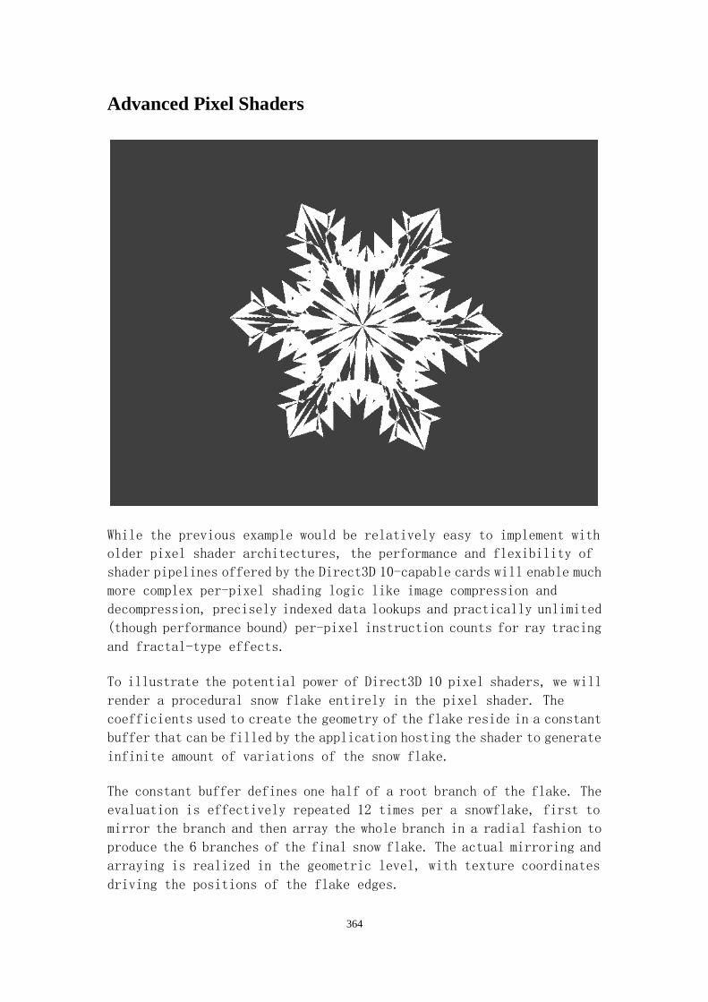
364

Advanced Pixel Shaders

While the previous example would be relatively easy to implement with

older pixel shader architectures, the performance and flexibility of

shader pipelines offered by the Direct3D 10-capable cards will enable much

more complex per-pixel shading logic like image compression and

decompression, precisely indexed data lookups and practically unlimited

(though performance bound) per-pixel instruction counts for ray tracing

and fractal-type effects.

To illustrate the potential power of Direct3D 10 pixel shaders, we will

render a procedural snow flake entirely in the pixel shader. The

coefficients used to create the geometry of the flake reside in a constant

buffer that can be filled by the application hosting the shader to generate

infinite amount of variations of the snow flake.

The constant buffer defines one half of a root branch of the flake. The

evaluation is effectively repeated 12 times per a snowflake, first to

mirror the branch and then array the whole branch in a radial fashion to

produce the 6 branches of the final snow flake. The actual mirroring and

arraying is realized in the geometric level, with texture coordinates

driving the positions of the flake edges.

365

To determine if a current pixel is inside the snow flake area or not,

triangles stored in the branch constant data are iterated by using a fill

algorithm that checks if the current pixel is inside a given triangle and

calculates a Boolean flag that stores whether the current pixel is in the

snowflake area.

The contributions of all the triangles to the pixel are combined together

with an XOR operation that switches the “insideness” flag of the current

pixel for each overlapping triangle area.

The following code implements the pixel shader used to rasterize the

snowflake:

//A triangle data type:

struct triang2

{

float2 p0, p1, p2;

}

// Establish a maximum number of snowflake triangles:

#define MAX_SF_TRIS 20

// The host application fills the snowflake data buffer

// with triangles:

cbuffer snowflakeData

{

int numFlakeTris;

triang2 flakeTris[MAX_SF_TRIS];

}

// Find the determinant of the matrix formed by u and v.

// Effectively determines if the vectors are clockwise

// or counterclockwise related to each other.

float det(float2 u, float2 v)

{

return u.x * v.y - u.y * v.x; //u cross v

}

// Find if a point is inside a given triangle:

bool PointInTriangle(float2 pnt, triang2 tri)

{

float2 v0, v1, v2;

float a1, a2, b1, b2;

// Test if the vector from p0 to pnt is inside the

366

// sector formed by p1-p0 and p2-p0:

v0 = tri.p0;

v1 = tri.p1 - tri.p0;


a1 = (det(pnt, v2)-det(v0, v2)) / det(v1, v2);

b1 = -(det(pnt, v1)-det(v0, v1)) / det(v1, v2);

// Test again from different vertex:

v0 = tri.p1;



a2 = (det(pnt, v2)-det(v0, v2)) / det(v1, v2);

b2 = -(det(pnt, v1)-det(v0, v1)) / det(v1, v2);

// We don't need to test the third sector separately,

// because if the point was in the first two sectors,

// it must already be inside the triangle.

//Just return the combined result of the first two tests:

if ((a1 > 0) && (b1 > 0) && (a2 > 0) && (b2 > 0))

return true;

else

return false;

}

// Vertex shader is omitted; it just transforms the

// geometry to projection space and passes thru the UV coords.

// The pixel shader for the snow flake.

// Input texture coordinates are used.

float4 snowflakePS(PS_In input) : SV_Target

{

//by default, we are not inside the flake:

bool inFlake = false;

//iterate over all flake triangles:

for (int i = 0; i < numFlakeTris; i++)

{

//utilize bitwise XOR to establish the flake shape:

inFlake ^= PointInTriangle(input.uv, flakeTris[i]);

}

367

// we draw the combined effect of all the flake triangles:

return

(inFlake?float4(1.0,1.0,1.0,1.0):float4(0.0,0.0,0.0,0.0))

;

}

Note that this is intentionally a heavy approach to rendering a snowflake.

In most applications, this method of rendering snowflakes would be an

order of magnitude more complex than is actually needed, because

snowflakes are usually very small in screen space and thus it would be

very wasteful to render it with all the detail that our approach generates.

That said, this technique does illustrate the flexibility and power of

the pixel shaders in Direct3D 10. More practical applications can and will

be developed that take advantage of them in common rendering tasks and

special effects.

Direct3D 10.1 Considerations For Procedural Shaders

Direct3D 10.1, the new feature baseline for graphics cards announced by

Microsoft in late 2007 and published in March 2008, gives programmers even

more power for creating shaders. Here, we take a look at some of the new

features that can benefit procedural shader programming.

Available Register Count Doubled to 32 per Shader Stage

More data can be transferred across the pipeline in a single pass, so more

complex shader logic is possible without having to divide processing into

smaller blocks at host program level. This ultimately results in higher

performance for complex shaders, regardless of the pipeline stage these

extra registers are used in.

You don’t need any special instructions to use the new register limits;

it is just possible to use more variables than before, if the HLSL code

is compiled with the new 4.1 profiles.

368

MSAA Enhancements

In D3D10.1, if pixels have attributes that vary across the pixel area,

said attributes can be evaluated per sample rather than per pixel like

in previous versions. This will greatly improve quality of procedural

shaders when the device is set to perform multi-sample antialiasing.

To enable the per-sample evaluation of the pixel shader, include the new

system-generated value SV_SampleIndex in the pixel shader parameters and

use it in the shader code to determine the current sample index. This

parameter is useful if a custom antialiasing pattern is to be implemented.

The shader will then run multiple times per pixel, based on the number

of samples per pixel in the destination render target.

If you need the destination sample position from the pixel shader, you

can use the intrinsic functions GetRenderTargetSamplePosition() and

GetRenderTargetSampleCount() to get information about where the current

pixel is to be written. This info can be used to optimize the quality of

ray-tracing type operations as well as discontinuous functions such as

the checker pattern earlier in this section of the book, by adjusting the

sampling positions given to the algorithms and taking multiple passes

without having to guess where the corresponding samples and pixels

actually are.

Custom Sample Resolving

It is possible to fetch individual samples of texels from a multi-sampled

render target texture. This is very useful if you want to perform tone

mapping of HDR data prior to combining the samples, as opposed to applying

tone mapping after the samples are combined (legacy way). This will help

avoid jagged edges that are an artifact of variance among the texel

samples’ intensities, and therefore improves visual quality

considerably in HDR scenarios. Strictly speaking, combining non-linear

(after tonemapping) samples is not physically correct way to weight sample

intensities, but in general usage the effect fools the eye quite

efficiently.

To load individual samples from a MSAA texture, first declare your input

MSAA texture in HLSL as Texture2DMS<float4, 4> where MS signifies

“multisampled”, float4 is the texture data type and the last parameter,

4, is the number of samples on a single texel of that texture. Then, use

369

the Load() method of the texture object; first parameter is the

unnormalized (that is, 0„textureWidth or 0„textureHeight), and the

second parameter is the index of the sample you want to fetch.

In conjunction with the Load() method, it is convenient to use the data

available from Texture.GetDimensions() in HLSL to determine the width and

height as well as the number of samples available in the source texture.

This method is not very expensive, contrary to what developers may

generally believe, since the graphics device has to carry this data

through the entire pixel pipeline anyway.

There are several other enhancements in D3D10.1 as compared to 10.0, but

the rest of them are not so specifically involved with procedural shaders

and more with the logistics of resources, performance improvements and

quality improvements. Nevertheless, it is likely worth taking a look at

all the new features of the 10.1 interfaces as they have been developed

by listening to – and catering to the needs of - actual graphics

developers.

"

370

Post Processing Pipeline

In this section, Wolfgang Engel provides a complete discussion of post

processing in a realtime environment. Starting with the basic concepts

and advancing through more advanced techniques and even providing several

commonly used techniques, this is a mandatory section for anyone entering

the post processing arena.

Introduction

A post-processing pipeline that applies post-processing effects to an

already rendered scene have become a de-facto standard in modern video

game graphics rendering. Post effects usually rely only on data that is

available in image space. Typical post-processing effects are:

Color Filters

High-Dynamic Range Rendering

Light Streaks

Depth of Field

Motion Blur

Miscellaneous Effects Snippets

The following text will present a description and an implementation of

these effects.

Color Filters

Color filters are by far the oldest post effect used in games. Impressive

examples are the Call of Duty and Medal of Honor series. The main idea

here is to give a winter scene -for example- a more grey-ish tint, a summer

scene a slight yellow tint or a scene in the jungle a slight

greenish/blueish tint. Color filters can also be triggered or changed

based on the player being in a specific area. When the player leaves one

area and goes to another, the color filters might change accordingly by

being linearly interpolated between areas.

Most of the time, color filters in a post-processing pipeline work on RGB

values. This color space is frequently used in most computer applications

since no transform is required to display information on the screen. It

is device dependent because different devices transform the linear-light

intensity to a nonlinear video signal by gamma correction.

371

Decent post-processing pipelines offer the following features:

Adding and multiplying Color

Color saturation control

Contrast control

Gamma control

Gamma Control

Physical light intensity values behave linearly - if two sources of light

shine on the same surface, their combined intensity is equal to the sum

of the intensities of the two sources. For this reason such values are

also known as "linear light" values. If we quantize linear light values

into fixed-width steps, we have physically uniform encoding - each step

increment has the same physical magnitude anywhere on the scale.

However when light values must be quantized using few bits, to minimize

banding artifacts the most efficient encoding is one which is perceptually

uniform - each step increment has the same perceptual magnitude anywhere

on the scale. Since human perception of brightness is non-linear (the

perceived brightness of combined sources is not equal to the sum of the

perceived brightness of separate sources), perceptually uniform and

physically uniform encodings are different.

To enable the use of 8-bit-per-channel display frame buffers without

noticeable banding, a standard nonlinear transfer function is defined for

converting linear light values into frame buffer values. After this

conversion, the frame buffer values are in a (roughly) perceptually

uniform space, also known as the sRGB color space [Stokes]. This is also

called gamma correction or sRGB encoding.

In other words, the main purpose of gamma correction or sRGB encoding of

colors is to optimize perceptual performance of a limited number of bits

in each component in RGB color space.

In addition to frame buffers, sRGB encoding is commonly used for many

textures stored in non-HDR formats. Textures authored by artists directly

such as color maps are commonly gamma corrected. Even modern 8-bit image

file formats (such as JPEG 2000 or PNG) default to the sRGB encoding.

The advantage of utilizing the available precision in a rendering pipeline

more efficiently by encoding images or framebuffers to sRGB needs to be

balanced against the fact that most color manipulation methods that are

applied in a renderer become physically non-linear.

372

By removing sRGB encoding or gamma correction, the result of dynamic

lighting, the addition of several light sources, shadowing, texture

filtering and alpha blending will look more realistic and advanced color

filters will provide predictable and consistent visual results (read also

[Brown]).

Background

The sRGB color space is based on the monitor characteristics expected in

a dimly lit office, and has been standardised by the IEC (as IEC 61966-1-2)

[Stokes]. The sRGB transfer functions are usually designed to be close

to a pure power function, which leads to a naming convention: the number

K which most closely matches the transfer function with X1/K is the gamma

value of the space. By this convention, sRGB is a gamma 2.2 space, and

linear light is a gamma 1.0 space. In theory, a pure power function would

work, but power functions have an infinite slope at zero, which causes

practical difficulties. For this reason, the transfer function has a

linear portion at the extreme low end. Figure 1 shows a power function:

Figure 1 - x2.2

Decent game engines receive color data from many sources (vertex color,

ambient occlusion color, textures etc.) and they blend those values in

different ways. To make the result of all those operations physically

373

linear, the sRGB encoding or gamma correction need to be removed before

any operation is applied.

Because the monitor expects a value that is sRGB encoded, a transfer

function that converts from gamma 1.0 to gamma 2.2 is applied to the

resulting color value before it is send to the framebuffer.

Gamma correction has a huge impact on the art workflow. Most game teams

nowadays setup their art pipeline so that all assets are viewed and created

with monitors and art packages assuming a gamma value of 2.2, whereas the

renderer of the game runs all dynamic lighting, color operations, texture

filtering (read more in [Brown]), and shadowing in linear gamma space.

This leads to visual inconsistencies between what the art team sees in

their tools and what the renderer produces as the end result. Most of the

time those inconsistencies are not as bad as the inconsistencies that

would have been introduced by running the renderer with sRGB encoding.

Some teams even switch to a workflow that assumes a linear gamma value

by re-adjusting and re-calibrating their LCD screens and their art tools.

Implementation

Most video game consoles and PC graphics cards are able to convert textures

internally from gamma 2.2 to gamma 1.0 while fetching the texture.

Additionally there is functionality available to convert color values

back to gamma 2.2 before they will be send to the display. That leaves

game developers with the challenge to manually convert color values to

gamma 1.0 that are fed to the renderer from other sources than a texture

or provide backward compatibility in case graphics hardware allows to

convert textures to gamma 1.0 without functionality to convert back to

gamma 2.2.

The equation to convert from sRGB to linear gamma is

374

Equation 1

Figure 2 shows the resulting curve of equation 1.

Figure 2- Transform from gamma 2.2 to linear gamma.

The equation to convert from linear gamma to gamma 2.2 is

375

Equation 2

Figure 3 shows the resulting curve of equation 2.

Figure 3 - Transform linear gamma to gamma 2.2.

The effect of the above equations closely fits a straightforward gamma

2.2 curve with a slight offset (read more in [Stokes]). Converting into

gamma 1.0 is done in HLSL like this:

float3 Color;

Color = ((Color <= 0.03928) ? Color / 12.92 : pow((Color +

0.055) / 1.055, 2.4))

376

Converting from linear gamma to gamma 2.2 can be done with the following

HLSL snippet:

float3 Color;

Color = (Color <= 0.00304) ? Color * 12.92 : (1.055 * pow(Color,

1.0/2.4) - 0.055);

Simplifying this equation leads to color inaccuracies of colors that are

smaller than 10 from the value range of 0..255 and therefore to banding

effects in dark textures.

Typical simplifications remove the condition that differs between values

lower than 0.03928 and values that are equal or higher than this number,

the following simplified code can be used to convert from gamma 2.2 to

gamma 1.0.

float3 Color;

Color = pow((Color + 0.055)/ 1.055, 2.4);

The code to convert from linear gamma to gamma 2.2 is:

Color = pow(1.055 * Color, 1.0/2.4)- 0.055;

Simplifying the gamma conversion even more, can be done by using a power

value of 1/2.2 to convert to gamma 2.2 and a power value of 2.2 to convert

to linear gamma.

All decent hardware offers gamma corrections from gamma 2.2 to gamma 1.0

and vice versa, while the conversion from gamma 2.2 to gamma 1.0 is only

supported for textures, while they are fetched. All other color values

need to be converted manually to gamma 1.0 in a pre-process or in the

renderer.

Before values are send to the monitor, the graphics hardware can convert

back to gamma 2.2. All conversions supported by hardware are free. ATI

graphics hardware supports piecewise linear approximations to the gamma

curve, while decent NVIDIA graphics hardware stick with the equations

above.

377

Contrast Control

Background

Contrast control is inherently a luminance-only operation. The following

equation produces good looking results:

Equation 3

Figure 4 visualizes this equation for a value range of 0..1.

Figure 4 - Visualization of a Contrast Operator based on a Cubic Polynomial

This contrast operator offers a visually more pleasant result than for

example using a power function. Similar to all the other color filters,

it assumes a gamma 1.0 color that is in the value range of 0..1. Therefore

it can only be used after tone mapping is applied.

378

In HSB color space, when choosing complementary colors, fully saturated

colors will offer the highest level of contrast. Choosing from tints or

shades within the hue family reduces the overall contrast of the

composition.

Implementation

A vectorized implementation of equation x is straightforward:

float3 Color = Color - Contrast * (Color - 1.0f) * Color *(Color

- 0.5f);

Color Saturation

Background

To remove color from an image, first its color values -that are already

in gamma 1.0- are converted to luminance values. Interpolating the then

desaturated copy of the image with the original color image offers a

seamless way to remove colors from an image.

The common way to transform a RGB value to luminance is taken from the

standard matrix such as specified in [ITU1990] to convert from CIE XYZ

color space to RGB. This matrix looks as shown in equation 4:

Equation 4

The Y component in the XYZ color space represents luminance. Thus, a

representation of luminance is obtained by computing a linear combination

of red, green and blue components according to the middle row of the

RGB-to-XYZ conversion matrix. Therefore luminance can be computed

following [ITU1990] as follows:

379

Equation 5

Implementation

The color saturation approach is build on the result of the color

conversion stage. Saturation is controlled by lerping between luminance

and the original color.

float Lum = dot(Color,float3(0.2126, 0.7152, 0.0722));

float3 Color = lerp(Lum.xxx, Color, Sat)

The variable Sat holds the value the user has chosen.

Color Changes

Background

The simplest color filters just add or multiply RGB values.

Implementation

Multiplying an incoming color value with a value for each color channel

and additionally adding a value to each of the color channels is done like

this.

float3 Color = Color * ColorCorrect * 2.0 + ColorAdd;

ColorCorrect and ColorAdd are vectors that hold three values for each of

the color channels.

High-Dynamic Range Rendering

In the real world, the difference between the brightest point in a scene

and the darkest point can be much higher than in a scene shown on a computer

display or on a photo. The ratio between highest and lowest luminance is

called dynamic range.

The range of light we experience in the real world is vast. It might be

up to 1012:1 for viewable light in everyday life, from starlight scenes

to sun-lit snow and up to a dynamic range of 104:1 from shadows to

380

highlights in a single scene. However, the range of light we can reproduce

on our print and screen display devices spans at best a dynamic range of

about 300:1 [Seetzen]. The human visual system is capable of a dynamic

range around 103:1 at a particular exposure. In order to see light spread

across a high dynamic range, the human visual system automatically adjust

it's exposure to light, selecting a narrow range of luminances based on

the intensity of incoming light. This light adaption process is delayed,

as you'll notice when entering a dark building on a sunny day, or vice

versa and is known as exposure adjustment.

Another property of the human visual system is visible, if extremely

bright areas are watched. The optic nerve can overload in such a situation

and produce an effect that is called glaring.

The human eye is made up of two main types of photo receptors, rods and

cones. As the luminance of an area being viewed decreases the rods shut

down and all vision is done through the cones. Although this isn't exactly

true since there are a small number of rods on at even very low luminance.

When cones become the dominant photo receptors there is a very slight shift

in colors to a more bluish range. This is due to the fact that there is

only one type of cone which is optimal at absorbing blues while rods come

in three types(red, green, blue). This shift is know as the Blue Shift.

Not only is there a shift to a bluish range but also since there are fewer

photons entering the eye there is more noise and there is a general loss

of detail.

Because of the restricted dynamic range of display systems, lighting

calculations are clamped to the narrow range of the device, so that the

images look washed out, over saturated, or much too dark on the monitor.

Additionally a display is not able to reproduce phenomena such as glare,

retinal burn and the loss of perception associated with rapid changes in

brightness across the temporal and spatial domains. Rendering systems

that attempt to sidestep these deficiencies are called high dynamic range

enabled systems or for short, HDR systems.

A HDR rendering system is keeping a high range of luminance values in the

whole rendering pipeline and it is compressing this high range to the small

range of luminance values that can be displayed with a process that is

called tone mapping. The tone mapping operator compresses HDR data into

the low-dynamic range the monitor is capable to display.

A common feature list of a HDR rendering system is:

Capable to handle data with a higher dynamic range than 0..1

381

Tone mapping operator to compress high-dynamic range values to the low dynamic range

the monitor expects

Light adaptation behavior similar to the human visual system

Glaring under intense lighting to imitate very bright areas that overload the optic nerve of

the eye

Blue shift and night view to account for the behaviour of the human visual system under

low lighting conditions

The following text will therefore discuss ways to store and keep data with

a high-dynamic range, a global tone mapping operator, temporal adaptation,

glare generation and the blue shift.

High-Dynamic-Range Data

To keep a high range of values the scene needs to be rendered with

high-dynamic range data. Then the post-processing pipeline has to

preserve the value range and precision of this data and compress it to

the lower dynamic range the monitor is capable to display with the tone

mapping operator.

Additionally a renderer and a post-processing pipeline should run in gamma

1.0 to make several light sources, all filtering, alpha blending, lighting

and shadowing operations linear regarding brightness. With gamma 1.0 the

color values will require an increased need for a higher range of values

compared to gamma 2.2 compressed RGB values.

A high dynamic range of values is usually considered as a higher range

of values than the 8:8:8:8 render target/texture format with its 8-bit

precision or its 256 deltas in each of its channels. In textures values

are even stored in much less than this due to memory constraints, while

graphics hardware is capable to handle a higher precision.

Therefore the challenge to preserve a high range of color and luminance

values is twofold. We have to store HDR data already in textures so that

scene rendering happens with HDR texture data and additionally keep this

value range and precision while running the data through the renderer and

the post-processing pipeline in render targets.

Storing High-Dynamic-Range Data in Textures

Decent video console systems, DirectX 9 and DirectX 10 conform graphics

cards allow the usage of DXT compressed textures. These formats compress

to 4-bit or 8-bit per pixel and offer a high compression for some loss

382

of quality. DXT5 for example quantizes the color channels to a palette

of four 16-bit (5:6:5) colors for each 4x4 block. In other words 16 points

in 3D space representing sixteen original colors in the block are replaced

with four colors from the palette. Two of these colors are stored in the

block and the other two are derived as a weighted sum of the former two.

This is the reason why DXT compressed normal maps look so bad - each 4x4

block is represented by only four different vectors.

The alpha channel is quantized to eight separate values for each 4x4 block.

The eight alpha values are distributed uniformly in a sub-range of the

0..1 range. The precision of the alpha channel is therefore higher

compared to the color channels.

One of the tricks of the trade to store HDR data in compressed textures

is done by utilizing the underlying idea of a texture format that is called

RGBE (known as Radiance RGBE format). It stores for each pixel a common

exponent in the alpha channel of the texture. With this format it is

possible to store a higher value range than 0..1 for the RGB channels by

packing those values into a single 32-bit texture (D3DFMT_A8R8G8B8 /

DXGI_FORMAT_R8G8B8A8_UINT), where RGB channels keep mantissas of the

original floating-point values and the alpha channel keeps the common

exponent. It was first described by Greg Ward [WardG] and it was

implemented in HLSL and applied to cube maps by Arkadiusz Waliszweski

[Waliszewski]. This format encodes floating point values to RGBE values

by dividing the floating point value through the exponent of the largest

value and then multiplying the result, that has a value range of [0.5 ..1.0]

with 255 to get it into a value range of [0..255]. The common exponent

is then stored in the alpha channel (this is were the E in RGBE is coming

from).

If one channel keeps values significantly smaller than the channel with

the greatest exponent, a loss of precision of this channel will happen.

Furthermore a RGBE texture can not be compressed, because compressing the

exponent would lead to visible errors.

Following the RGBE texture format, DirectX 10 now offers a

DXGI_FORMAT_R9G9B9E5_SHAREDEXP format that has a better resolution than

RGBE that is typically stored in 8:8:8:8 textures. Similar to RGBE the

new format can not be compressed.

383

Compressing HDR Textures

Based on RGBE, most decent HDR texture formats keep the exponent value

separate from the values in the RGB channels. This way the values in the

RGB channels can be compressed for example in a

DXT1/DXGI_FORMAT_BC1_UNORM texture and the exponent can be stored

uncompressed in a quarter size L16 texture. This also allows filtering

the value in the compressed texture with hardware.The reduction in size

of the exponent L16 texture can be justified by the fact that the DXT1/

DXGI_FORMAT_BC1_UNORM compressed texture represents the original

uncompressed 16 color values by only four color vectors. Therefore storing

exponents only for a quarter of the colors of the original uncompressed

texture should not lead to a visible quality decrease. A

DXT1/DXGI_FORMAT_BC1_UNORM +L16 HDR format should end up at about 8-bit

per pixel instead of the 32-bit of the original RGBE texture; similar to

a DXT5/DXGI_FORMAT_BC5_UNORM compressed texture.

Higher compression of HDR data can be achieved by storing a common scale

value and a bias value for all the RGB channels in a texture by utilizing

unused space in the DXT1/DXGI_FORMAT_BC1_UNORM header. This compresses

data to 4-bit per pixel (read more about HDR textures in [Persson]).

Gamma correcting HDR Textures

All decent hardware can remove the gamma correction (convert from gamma

2.2 to gamma 1.0) from textures while they are fetched. In Direct3D 10,

sRGB encoding is handled by using one of the UNORM_SRGB formats for the

shader resource or render target view. When such formats are used,

conversions into linear space (on read) or from linear space (on write)

are handled automatically. Unlike previous versions of Direct3D, D3D10

requires that the hardware perform sRGB conversions in the correct order

relatively to filtering and alpha-blending operations.

In case a HDR texture format is used a common scale and bias value stored

in the header of the file or an exponent value in a separate texture need

to be stored assuming a gamma 1.0 space.This means that a texture tool

needs to convert the texture first to gamma 1.0, then split up the values

into a mantissa and an exponent and than convert the mantissa part -that

is the RGB part- back to gamma 2.2. This way the exponent or the bias and

scale values stays in gamma 1.0.

384

According to the roadmap for the upcoming features in DirectX, Microsoft

will provide a HDR texture that takes 8-bit per pixel and offers gamma

control.

Keeping High-Dynamic-Range Data in Render Targets

To preserve the precision of the data generated by the previous render

operations, the post-processing pipeline needs to use render targets with

enough precision. The most important render target here is the very first

render target that is used to render the scene into. This render target

is usually expected to support alpha blending, multi-sampling and

filtering and it determines how much precision is available in the

following stages.

On DirectX 9 compatible graphics cards, there is a 16-bit per channel

floating-point render target format and a 10:10:10:2 render target format

available.

Graphics cards that support the 10:10:10:2 render target format support

alpha blending and multi-sampling of this format (ATI R5 series). Some

DirectX 9 graphics cards that support the 16:16:16:16 format support alpha

blending and filtering (NVIDIA G7x), others alpha blending and

multi-sampling but not filtering (ATI R5 series).

Only the latest DirectX 10 compatible graphics cards (NVIDIA G8x) supports

alpha blending, filtering and multi-sampling on a 16:16:16:16 render

target.

The new DXGI_FORMAT_R11G11B10_FLOAT render target format available in

DirectX 10 compatible graphic cards offers the best of both DirectX 9

render target formats, because it offers the memory bandwidth of the

10:10:10:2 format with more precision and source alpha blending,

filtering and multi-sampling support. If more alpha blending

functionality is required a 16-bit primary render target would be

necessary.

The XBOX 360 supports a render target format that is called 7e3, which

is a 10:10:10:2 floating-point EDRAM render target format (the

corresponding resolve render target on this platform is a 16:16:16:16

floating point format). This render target format is re-configurable, so

that the user can select the supported value range and with it the

precision [Tchou]. A common value range here is 0..4.

385

The PS3 supports a 16:16:16:16 floating point render target format and

a 8:8:8:8 render target format. In case the bandwidth consumption of a

16:16:16:16 floating point render target is too high, a 8:8:8:8 render

target format needs to be utilitzed to store HDR data.

8:8:8:8 Render Targets

If the target hardware platform only supports 8-bit per channel render

targets with multi-sampling, filtering and alpha blending or a specific

situation requires this render target format, using an alternative color

space is a good option to preserve precision.

A requirement list for an alternative color space is as follows:

1. Needs to encode and decode fast enough

2. Needs to be bilinear filterable without encoding / decoding

3. Needs to work with a blur filter without encoding / decoding

If the requirements 2 and 3 are met, encoding / decoding only needs to

be done once for the whole post-processing pipeline. In that case the

conversion from RGB in gamma 1.0 to the alternative color space needs to

be done once while rendering into the main render targets and then the

conversion back to RGB only needs to happen once at the end of the

post-processing pipeline.

Color Space #of cycles to

encode

Bilinear

filtering

Blur

filter

Alpha

blending

RGB - Yes Yes Yes

HSV 34 No No No

CIE Yxy 11 Yes Yes No

L16uv (based on Greg Ward's

LogLuv) 19 Yes Yes No

RGBE 13 No No No

Table 1 - Overview alternative color spaces

The number of cycles are measured in ATI's RenderMonkey and can only

provide a rough idea on how fast the encoding algorithm works.The blur

filter was a simple four tap filter with extended offsets.

386

HSV would be a good choice in a game engine that is build around it. The

performance of encoding in HSV might be improved by using a look-up table.

This color space does not support bilinear filtering or a blur filter,

although bilinear filtering still might look good enough. HSV would be

a good choice in a game engine that is build around it.

CIE Yxy is quite often used in a post-processing pipeline to decode/encode

luminance for the tone mapping operators. It encodes reasonably fast. CIE

Yxy supports bilinear filtering and it also supports applying a blur

filter.

The same is true for L16uv. This is based on Greg Ward's LogLuv color space,

that is used to compress HDR textures. Instead of storing a logarithmic

luminance value, the luminance is distributed in the L16uv color space

over two 8-bit channels of a 8:8:8:8 render target.

The last color space is RGBE. This is often used as an intermediate format

for HDR textures. It does not work well with bilinear filtering, blurring

and would therefore require a decoding and encoding effort every time it

would be blurred.

Underlying this comparison, the CIE Yxy or the L16uv color space would

be the most efficient way to encode and decode HDR data in all four channels

of a 8:8:8:8 render target. Both are very similar in performance.

All alternative color spaces above do not support alpha blending.

Therefore all blending operations still have to happen in RGB space.

Implementation

An implementation of a high-dynamic range renderer that renders into

8:8:8:8 render targets might be done by differing between opaque and

transparent objects. The opaque objects are stored in a buffer that uses

the CIE Yxy color model or the L16uv color model to distribute precision

over all four channels of this render target. Transparent objects that

would utilize alpha blending operations would be stored in another 8:8:8:8

render target in RGB space. Therefore only opaque objects would receive

a better color precision.

To provide to transparent and opaque objects the same color precision a

Multiple-Render-Target consisting of two 8:8:8:8 render targets might be

used. For each color channel bits 1-8 would be stored in the first render

target and bits 4 - 12 would be stored in the second render target (RGB12AA

387

render target format). This way there is a 4 bit overlap that should be

good enough for alpha blending.

Tone Mapping Operator

Most post-processing pipelines use a tone mapping operator that was

developed by Erik Reinhard [Reinhard]. The underlying idea for the tone

mapping operator is based on Ansel Adams zone system, used in his black

and white photographs. Adam's defined 11 zones of brightness / luminance

and printed them on a card for reference when he is out in the wilderness

to make his photos. While shooting his photo, he made notes on the picture

that he is going to take. He scribbled the picture into his notebook with

roman numbers for the zones he can see for certain areas.

Back in his dark room he tried to re-create the luminance values in the

photo that he saw by using his card with the zones and the blueprint from

his notebook.

In the spirit of Ansel Adams approach, we create a luminance copy of the

picture and use this copy to measure an average luminance of the current

frame. We do not use a card with 11 different luminance zones, but we use

at least an average luminance value that maps by default to zone 5 of the

zone system. This is called the middle grey value and it is the subjective

middle brightness value that is ~18% reflectance on the print. Then we

adjust the luminance of the resulting color image with the average

luminance value we measured and with the middle grey value.

While Ansel Adams tried to make up for the difference in the range of

possible brightness values of the real-world compared to what was possible

to store at his time on photo paper, we try to make up for the difference

in the range of possible brightness and color values of what is generated

by the renderer compared to what is possible to display on an average

monitor.

This process is called tone mapping. The tone mapping operator compresses

data with a high-dynamic range to low-dynamic range data. Tone mapping

is one of the last stages in a post-processing pipeline, to assure that

all operations can be done on the full range of values.

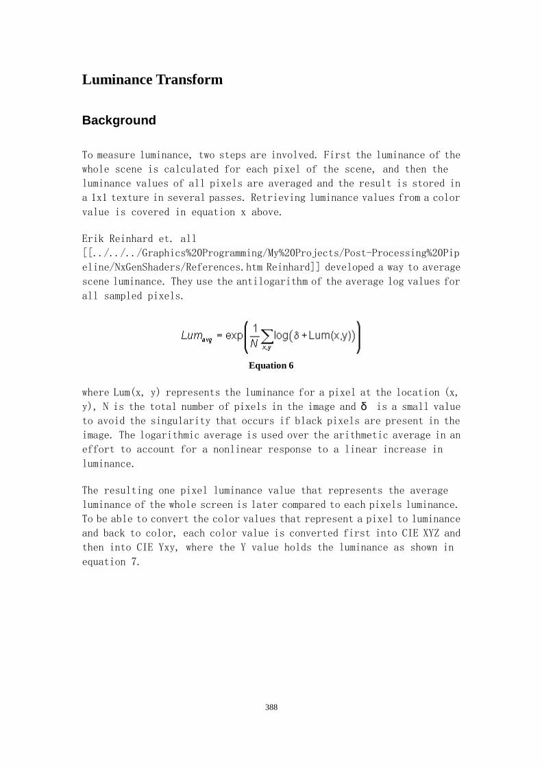
388

Luminance Transform

Background

To measure luminance, two steps are involved. First the luminance of the

whole scene is calculated for each pixel of the scene, and then the

luminance values of all pixels are averaged and the result is stored in

a 1x1 texture in several passes. Retrieving luminance values from a color

value is covered in equation x above.

Erik Reinhard et. all

[[../../../Graphics%20Programming/My%20Projects/Post-Processing%20Pip

eline/NxGenShaders/References.htm Reinhard]] developed a way to average

scene luminance. They use the antilogarithm of the average log values for

all sampled pixels.

Equation 6

where Lum(x, y) represents the luminance for a pixel at the location (x,

y), N is the total number of pixels in the image and δ is a small value

to avoid the singularity that occurs if black pixels are present in the

image. The logarithmic average is used over the arithmetic average in an

effort to account for a nonlinear response to a linear increase in

luminance.

The resulting one pixel luminance value that represents the average

luminance of the whole screen is later compared to each pixels luminance.

To be able to convert the color values that represent a pixel to luminance

and back to color, each color value is converted first into CIE XYZ and

then into CIE Yxy, where the Y value holds the luminance as shown in

equation 7.

389

Equation 7

Then this luminance value can be adjusted and values can be converted back

via CIE Yxy values back to RGB following equation 8.

Equation 8

Implementation

To transform the color images into one luminance value that represents

the luminance of the whole screen, the color value is first converted based

on part of equation x that stands in brackets. To convert the color values

to luminance values the same equation is used as for the color saturation

effect:

const float3 LUMINANCE = float3(0.2125f, 0.7154f, 0.0721f);

const float DELTA = 0.0001f;

float fLogLumSum = 0.0f;

fLogLumSum += log(dot(tex2D(ToneMapSampler, TexCoord.xy +

float2(-1.0f * TexelSize, -1.0f * TexelSize)).rgb, LUMINANCE)

+ DELTA);


float2(-1.0f * TexelSize, 0.0f)).rgb, LUMINANCE) + DELTA);

390


float2(-1.0f * TexelSize, 1.0f * TexelSize)).rgb, LUMINANCE)

+ DELTA);

This code fetches the color render target nine times. Depending on the

difference in size between the render target that this codes uses to read

from and the render target where it writes into, more or less texels have

to be fetched. The task of the following stages is to downsample the result

of this pass by halfing the render target sizes. If this pass renders into

a 128x128 render target, the following stages will downsample to 64x64,

16x16, 4x4, 1x1 by fetching always 16 texels from the render target they

read. The very last render target will then apply the exponential function

of equation x like this:

float fSum = 0.0f;

fSum += tex2D(ToneMapSampler, TexCoord.xy + float2(1.5f *

TexelSize, -1.5f * TexelSize)).x;


TexelSize, -0.5f * TexelSize)).x;


TexelSize, 0.5f * TexelSize)).x;

...

return fSum = exp(fSum / 16.0f);

...

Each pixel in the target render target represents with a 16-tap shader

16 pixels in the source render target.

The drawback of converting a color value into a luminance value by

multiplying it with the LUMINANCE constant described above is, that it

is not possible to convert it back to color afterwards. To be able to

compare the average luminance value gained through equation 6 with the

luminance of each pixel and adjusting the luminance of each pixel with

this luminance value, we need to convert each pixel to luminance as shown

in equation 7. Then we are able to adjust its luminance value and later

we can convert back to color following equation 8. Converting a pixel color

into luminance can be done with the following source code:

// RGB -> XYZ conversion

// http://www.w3.org/Graphics/Color/sRGB

// The official sRGB to XYZ conversion matrix is (following

ITU-R BT.709)

// 0.4125 0.3576 0.1805

// 0.2126 0.7152 0.0722

391

// 0.0193 0.1192 0.9505

const float3x3 RGB2XYZ = {0.5141364, 0.3238786, 0.16036376,

0.265068, 0.67023428, 0.06409157, 0.0241188, 0.1228178,

0.84442666};

float3 XYZ = mul(RGB2XYZ, FullScreenImage.rgb);

// XYZ -> Yxy conversion

float3 Yxy;

Yxy.r = XYZ.g;

// x = X / (X + Y + Z)

// y = X / (X + Y + Z)

float temp = dot(float3 1.0,1.0,1.0), XYZ.rgb);

Yxy.gb = XYZ.rg / temp;

Converting the resulting luminance value back to color the following code

can be used:

// Yxy -> XYZ conversion

XYZ.r = Yxy.r * Yxy.g / Yxy. b;

// X = Y * x / y

XYZ.g = Yxy.r;

// copy luminance Y

XYZ.b = Yxy.r * (1 - Yxy.g - Yxy.b) / Yxy.b;

// Z = Y * (1-x-y) / y

// XYZ -> RGB conversion

// The official XYZ to sRGB conversion matrix is (following

ITU-R BT.709)

// 3.2410 -1.5374 -0.4986

// -0.9692 1.8760 0.0416

// 0.0556 -0.2040 1.0570

const float3x3 XYZ2RGB = { 2.5651,-1.1665,-0.3986, -1.0217,

1.9777, 0.0439, 0.0753, -0.2543, 1.1892};

392

The RGB->Yxy and the Yxy->RGB conversions are used in the bright-pass

filter and the tone-mapping operator. The following section describes how

a tone mapper adjusts the luminance values of single pixels with the help

of the average luminance value. The luminance value stored in the variable

LumImage represents the luminance of an individual pixel converted with the

code above and the luminance value stored in the variable LumAverage

represents the luminance converted with the chain of downsampling render

targets and the constant LUMINANCE vector.

Range Mapping

Background

With the average luminance in hand, the luminance of the current pixel

can be scaled with the middle grey value like this:

Equation 9

Applying this equation to all pixels will result in an image of relative

intensity. Assuming the average luminance of a scene is 0.36 and the middle

grey value is following Ansel Adams subjective middle brightness value

of 0.18, the luminance value range of the final image would be half the

value range of the original image.

Depending on day time and weather conditions, the middle grey value needs

to be chosen differently. This might happen via keyframed values that

depend on time of day and weather conditions or it might happen dynamically.

[Krawczyk] uses the following equation to generate a middle grey value

dynamically for videos.

Equation 10

This function simply blends between a set of key values that have been

empirically associated with different luminance levels. The following

figure 5 visualizes equation 9 with an average luminance value range of

0..1 and a middle grey value of 0.18.

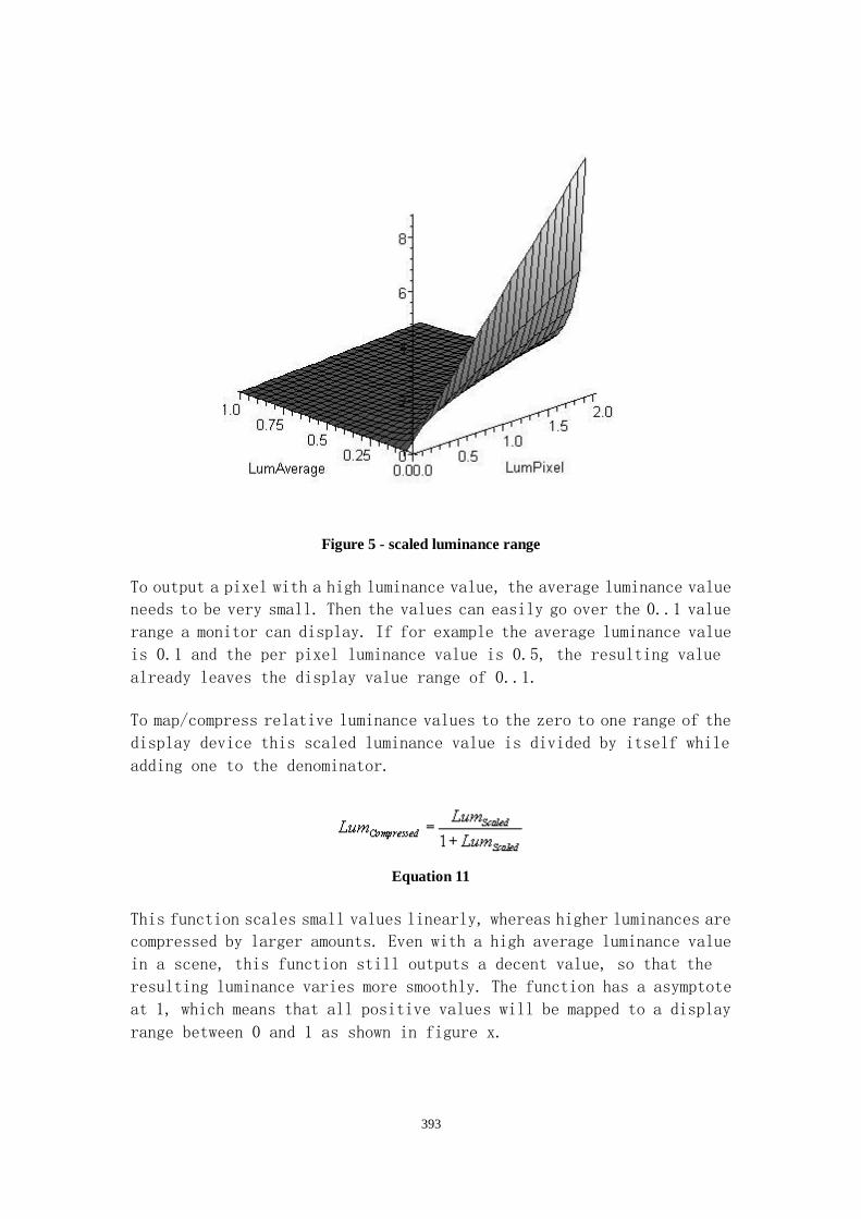
393

Figure 5 - scaled luminance range

To output a pixel with a high luminance value, the average luminance value

needs to be very small. Then the values can easily go over the 0..1 value

range a monitor can display. If for example the average luminance value

is 0.1 and the per pixel luminance value is 0.5, the resulting value

already leaves the display value range of 0..1.

To map/compress relative luminance values to the zero to one range of the

display device this scaled luminance value is divided by itself while

adding one to the denominator.

Equation 11

This function scales small values linearly, whereas higher luminances are

compressed by larger amounts. Even with a high average luminance value

in a scene, this function still outputs a decent value, so that the

resulting luminance varies more smoothly. The function has a asymptote

at 1, which means that all positive values will be mapped to a display

range between 0 and 1 as shown in figure x.

394

Figure 6 - Reinhard's simple tone mapping operator

However in practice the input image does not contain infinitely large

luminance values, and therefore the largest display luminances do not

always reach 1 or more. In addition it might be artistically desireable

to let bright areas burn out in a controlled fashion. Reinhard achieves

this effect by blending the previous transfer function with a linear

mapping, yielding the following tone mapping operator:

Equation 12

Equation 12 introduces a new parameter, White, which denotes the smallest

luminance value that will be mapped to white. By default, this parameter

is set to the maximum world luminance. For low-dynamic-range images,

setting White to smaller values yields a subtle contrast enhancement.

In other words: White minimizes the loss of contrast when tone mapping

a low dynamic rnage image. This is also called whitepoint clamping. Figure

7 and figure 8 show equation 12 with a middle grey value of 0.18 and a

value range of 0..4 for the luminance of individual pixels in a scene.

395

Figure 7 - Advanced Tone Mapping operator with a White value of 2

Figure 8 - Advanced Tone Mapping Operator with a White value of 6

Figure 8 below figure 7 shows that the equation becomes more similar to

the simple tone mapping operator if the White value is increased and if

396

it is decreased it approaches more the form of the simple scaling function

in equation 9.

Implementation

The source code for the advanced tone mapping operator described in

equation 12 and visualized in figures 7 and 8 is very straightforward:

// Map average luminance to the middlegrey zone by scaling

pixel luminance

// raise the value range a bit ...

float LumScaled = Yxy.r * MiddleGray / (AdaptedLum.x +

0.001f);

// Scale all luminance within a displayable range of 0 to 1

Yxy.r = (LumScaled * (1.0f + LumScaled / White))/(1.0f +

LumScaled);

The first line follows equation 9 expecting the RGB-to-Yxy converted

luminance value in the variable Yxy.r. This was shown in the paragraph

named "Luminance Transform" above. The small delta value should prevent

divisions through 0. In the second source code line, the value in White

is already multiplied with itself before it is send down to the pixel

shader.

Light Adaptation

Because we measure the luminance every frame, we can re-use the data to

mimic the light adaptation process of the eye. Light adaptation happens

if bright to dark or dark to bright changes happen, for example if we leave

a dark room to go into a bright outdoor area or vice versa.

The retina contains two types of photoreceptors, rods and 6 to 7 million

cones. The rods are more numerous, some 120 million, and are more sensitive

to light than the cones. However, they are not sensitive to color.

The daylight vision (cone vision) adapts much more rapidly to changing

light levels, adjusting to a change like coming indoors out of sunlight

in a few seconds. Like all neurons, the cones fire to produce an electrical

impulse on the nerve fiber and then must reset to fire again. The light

adaptation is thought to occur by adjusting this reset time.

397

The rods are responsible for our dark-adapted, or scotopic, vision. They

are more than one thousand times as sensitive as the cones and can be

triggered by individual photons under optimal conditions. The optimum

dark-adapted vision is obtained only after a considerable period of

darkness, say 30 minutes or longer, because the rod adaption process is

much slower than that of the cones.

In a game scenario it should not make sense to add a 30 minute light

adaptation sequence when the main character comes from a very bright

outdoor environment to a very dark indoor environment or a 3 seconds

adaptation time to a racing game (in real-life the driver would for example

try to prevent himself from being blinded by the sun to get around any

adaptation time). Therefore any approximation needs to be very rough for

game play reasons and most games will end up with a subtle light

adaptation.

To simulate the eyes reaction to temporal changes in lighting conditions

an adapted luminance value replaces the average luminance value in

previous equations.

As the average luminance changes the adapted luminance should drift in

pursuit. In the event of stable lighting conditions the adapted and

average luminance should become equal, representing fully adjusted eyes.

This behavior can be achieved by an exponential decay function

[Pattanaik]:

Equation 13<center>

Where dt is the time step between frames and tau is the adaptation rate. Human eyes adjust to light or dark conditions at different rates. When

moving from a dark building to a sunny courtyard your eyes will adapt at

a noticeably rapid rate. On the other hand, when moving from a sunny

courtyard into a dark building it can take between ten and thirty minutes

to fully adapt. This lack of symmetry is due to the rods (responsible for

scoptic vision or dark-adapted vision) or cones of the retina dominating

perception in dark or light conditions respectively. With this in mind

tau can be found by interpolating between the adaptation rates of the rods

and cones.

<center> <center>

<center>Equation 14

398

Assigning a value of 0.2 to tau for the rods and 0.4 to tau for the cones

gives pleasing results in a typical scenario.

Luminance History Function

Background

To prevent very short luminance changes from influencing the light

adaptation the change of the average luminance of a scene can be stored

over 16 frames for example to only allow light adaptation if all average

luminance values increased or decreased over the last 16 frames. Equation

x compares the average luminance values of the last 16 frames with the

current adapted luminance. If all the values in the last 16 frames are

bigger or equal to the current adapted luminance value, light adaptation

will happen. If all those values are smaller, light adaptation will also

happen. If some of the 16 values of the last 16 frames are pointing in

different directions, no light adaptation will happen (see also [Tchou]).

Equation 15

Equation 15 looks at first sight quite complex, but an implementation only

needs to run once per frame.

Implementation

The luminance history of the last 16 frames can be stored in a 4x4 render

target. This render target is then read with a shader that holds equation

15. Depending on the history of the last 16 frames, the adapted luminance

value of the current frame will be returned or the adapted luminance of

the previous frame.

float4 LumVector; // holds four luminance values

float4 zGreater; // holds the result of one comparison

float4 CompResult; // holds the result of all four comparisons

399

LumVector.x = tex2D(ToneMapSampler, TexCoord.xy +

float2(1.5f * TexelSize, -1.5f * TexelSize)).x;

LumVector.y = tex2D(ToneMapSampler, TexCoord.xy +

float2(1.5f * TexelSize, -0.5f * TexelSize)).x;

LumVector.z = tex2D(ToneMapSampler, TexCoord.xy +

float2(1.5f * TexelSize, 0.5f * TexelSize)).x;

LumVector.w = tex2D(ToneMapSampler, TexCoord.xy +

float2(1.5f * TexelSize, 1.5f * TexelSize)).x;

zGreater = (AdaptedLum <= LumVector);

CompResult.x = dot(zGreater, 1.0f);

...

// this is repeated four times for all 16 pixels

// if the result here is 16, all the values in the 4x4 render

target are bigger than the current average luminance

// if the result here is 0, all the values are smaller than

the current average luminance

CompResult.x = dot(CompResult, 1.0f);

if(CompResult.x >= 15.9f || CompResult.x <= 0.1f)

{

// run light adaptation here

...

}

else

{

// use luminance value from previous frame

...

}

Glare

Glare generation is accomplished by a bright pass filter followed by an

area convolution to mimic the overloading of the optic nerve in the eye

under very bright lighting conditions.

The bright pass filter compresses the dark parts of a scene so that the

bright areas are emphasized. The remaining bright areas are then blurred

with a Gaussian convolution filter. By blending the end result of those

two stages with the already tone-mapped final image an effect is achieved

400

similar to the dodging and burning used by Ansel Adams to brighten or

darken parts of black and white photographs; just with color images.

Bright pass filter

To be consistent with the rest tone mapping stage, the bright pass filter

uses a tone mapping operator to compress darker areas, so that the

remaining image consists of relatively bright areas. The basis for this

operator is again Reinhard's tone mapping operator as shown in equation

x.

Equation 16<center>

Figure 9 shows the resulting curve of the bright pass filter.

<center>

Figure 9 - Bright pass filter with a threshold of 0.5 and an offset value of 1.0.

The parameter T -Threshold- in the bright pass tone mapping operator moves

the whole curve into the -y direction, while the parameter O -Offset-

changes the flow of the curve. Increasing the value of O makes the curve

401

steeper, which means it is more sensitive to light changes and decreasing

makes it more shallow, so that it is less sensitive to light changes. The

bright pass filter has its own white value, which is set to 4 in figure

9.

Blur

A blur filter based on a simplified algorithm developed by Gauss is used

to blur the result of the bright pass as shown in figure x:

Figure 10 - Gaussian blur filter

This Gauss filter blurs 2D images by sampling a circular neighborhood of

pixels from the input image and computes their weighted average.

Equation 17

This filter can be rearranged and made separable as shown in equation 18:

402

Equation 18

Where ζ is the standard deviation of the Gauss filter and x and y are

the coordinates of image samples relative to the center of the filter.

Factorizing the equation this way lets us compute the Gauss filter with

a series of 1D filtering operations. Combining for example a weighted sum

of a column of 13 pixels centered around the current pixel with a weighted

sum of a row of 13 pixels centered around the same pixel will mimic a 25-tap

filter.

The bright-pass filter and the Gauss filter can be applied to very small

render targets to save performance. Typically quarter-size or a

sixteenth-size render targets are used here. These filters do not

necessarily applied in the order presented here. Bluring a small image

with a Gauss filter and then applying the bright-pass filter later is also

possible and sometimes favourable if the blurred image can be re-used for

other effects like Depth of Field.

Night Tonemapping / Blue Shift

The tone mapping operators discussed so far all assume that the image

represents a scene under photopic viewing conditions, i.e., as seen at

normal light levels. For scotopic scenes, i.e. very dark scenes, the human

visual system exhibits distinctly different behavior. In particular,

perceived contrast is lower, visual acuity is lower, and everthing has

a slightly blue appearance.

A night tone mapping operator reduces brightness and contrast,

desaturates the image, adds a blue shift and reduces visual acuity (read

more in [Shirley]).

A typical approach starts by converting the image from RGB to XYZ. Then,

scotopic luminance V may be computed for each pixel:

Equation 19

To tint the scotopic luminance V with a blue shift, the single channel

image is multiplied with the blue shift color.

403

Equation 20

The night view can then be achieved by a simple linear blend between the

actual scene and this night color.

Light Streaks

Background

Light streaks are the result of light scattering as it passes through a

lens or aperture. Cracks, scratches, grooves, dust, and lens

imperfections cause light to scatter and diffract. Eyelashes and even the

eye's lens can diffract and scatter incoming light. The more intense the

incoming light is relative to the surrounding ambient light level, the

more perceivable the scattering will be. Light scattering is therefore

an important visual cue that help the viewer discern the relative

brightness of light sources in comparison to their surroundings

[Spencer].

Painting light streaks would be done with a brush by pressing a bit

harder on the common point and releasing the pressure while moving the

brush away from this point. This is very similar to what a light streak

filter is doing while it is "smearing" a bright spot into several

directions, so that it looks like a star or a cross consisting of two or

more arms.

A common implementation for a common cross-like light streak is based on

a 4-tap kernel. It runs in two passes per streak over the whole render

target (read more in [Kawase][Oat]).

The first pass starts at the pixel being rendered as shown in Figure 11.

404

Figure 11 - Light Streak filter passes

The second pass than samples at every fourth neighboring pixel in the

direction of the streak. Both passes are used to generate one streak

resulting in 8 passes for light streaks in form of a cross. Every

additional strike direction requires then 4 additional passes. This idea

can be simplified on hardware that supports more than four texture fetches

at once by creating a 7-tap filter that does two streaks at once like this.

Figure 12 - One Pass Light Streak

The obvious drawback is that especially the center of the resulting streak

is not sampled as often and therefore does not look as soft. To make up

for this, a blur filter can be run over the resulting image. In case of

a cross like light streak pattern about 4 - 6 passes will result in good

looking results.To adjust the strength of the streaks the samples are

weighted differently with the following equation.

Equation 21

With the 7-tap approach the value in is used in both directions from the

third sampling point on. To be able to bend the streak filter in any

405

direction, Oat [Oat] added an orientation vector that is used to show the

direction from which the samples need to be taken like this.

Equation 22

The variable SC holds the texture coordinate in T, b holds the power value

of four or seven -depending on how many fetches are done in the pixel

shader-, V is the vector that represents the streak direction vector, the

variable TxSize holds the texel size (1.0f / SizeOfTexture) and the sample

number in s. As shown by Oat storing orientation vectors in a look-up

texture offers interesting effects like light streaks that follow the

bending of the windshield.

Implementation

Most light streak effects consist of two or three light streaks that form

a star like pattern. The following code shows how to draw

one of those light streaks in one pass.

float4 Color = 0.0f;

// get the center pixel

// Weights represents four w values from equation 21. It is

calculated on the application level and send to the pixel

shader

Color = saturate(Weights.x) * tex2D(RenderMapSampler,

TexCoord.xy);

// setup the SC variable of equation 22

// the streak vector and b is precomputed and send down from

the application level to the pixel shader

float2 SC = LightStreakDirection.xy * b * TexelSize.xy;

// take sample 2 and 4 (figure 12)

Color += saturate(Weights.y) * tex2D(RenderMapSampler,

TexCoord.xy + SC);

406

Color += saturate(Weights.y) * tex2D(RenderMapSampler,

TexCoord.xy - SC);


SC += SC;

Color += saturate(Weights.z) * tex2D(RenderMapSampler,

TexCoord.xy + SC);

Color += saturate(Weights.z) * tex2D(RenderMapSampler,

TexCoord.xy - SC);


SC += SC;

Color += saturate(Weights.w) * tex2D(RenderMapSampler,

TexCoord.xy + SC);

Color += saturate(Weights.w) * tex2D(RenderMapSampler,

TexCoord.xy - SC);

return saturate(Color);

By picking antipodal texture coordinates the effort to setup the texture

fetches is minimized. To emphasize the light streak, the whole effect can

be repeated with different b values for each pass.

Depth of Field Filter

In photography and movies, the zone of acceptable sharpness (also called

in focus) is referred to as the depth of field. The zone in front of the

depth of field and after depth of field appears to be blurred in movies

and photos, which is caused by the physical properties of camera lenses.

While possibly considered undesireable, it is now a commonly used tool

in bringing a viewer's attention to specific areas of a scene, enhancing

the visual experience.

A depth of field filter mimics the zone of acceptable sharpness of camera

lenses by blurring everything outside this zone. On a per-pixel basis the

distance between the camera and the objects in a scene is compared to the

distance between the camera and the near and far blur plane as shown in

Figure 13.

407

Figure 13 - Depth of Field filter

This figure shows how the car on the left will be blurred because it is

far away from the camera than the far blur plane, whereas the car on the

right will only be partially blurred because it is nearer to the camera

than the near blur plane. The car in the middle is in the depth of field.

The main challenge of implementing a depth of field filter is converting

the depth value of the pixel that should be drawn to camera space, so that

they can be compared to the near and far blur plane that are in camera

space as well.

To derive an equation that converts depth buffer values into camera space,

we must first understand how these values are obtained. Below is a standard

left-handed row-major perspective projection matrix, which is used to

transform camera space coordinates to clip space (NDC).

408

Equation 23

The only difference compared to the left-handed projection matrix version

is, that the left-handed version negates ZnQ in the third column. Some

graphics engines based on a right-handed coordinate system have positive

values to specify the near and far clipping plane. In this case the

left-handed version would be still applicable.

Equation 24.1 shows the full equation that results from multiplying a 4D

homogenous vector with the third column of the projection matrix above.

Equation 24

Equation 24.2 shows how to factor in the homogenous divide by w, in the

case of the above matrix w =z. This is the final depth buffer equation.

Solving for z leads to equation 24.3 that can be used to back-transform

depth buffer values into camera space (read more in [Scheuermann] and

[Gillham]).

Instead of fetching the depth buffer to calculate the camera space

distance of the pixel, the camera space depth value of each pixel can be

stored in the alpha channel of the render target while rendering the scene.

This approach would not cooperate with alpha blending well. Additionally

many post-processing effect might utilize camera space depth values as

well, so it is expected to be re-used between several effects.

With the ability to determine the distance from the camera of each pixel

that needs to be written into the frame buffer, the camera distance of

a pixel can now be compared to where the focus of the camera is and to

the range of the depth of field effect. Based on the result of this

comparison the pixel color can be chosen from a blurred or an unblurred

image emulating the blurring effect that happens outside of the depth of

field.

Picking the blurred or unblurred image is done by linearly interpolating

between those based on the variable s like this:

409

Equation 25

Mimicing the focus of a real camera, the camera space range of the depth

of field can be calculated like this:

Equation 26

The Range value fades in and out into the near and far blur plane as shown

in Figure 14.

Figure 14 - Result of different Range values

This figure shows a Focus value of 0.5 and Range values between 0 and 4.

The y axis represents the resulting value s that is used to linearly

interpolate between the blurred and the original image. A value of 1 means

the pixel color is picked from the blurred image and a value of 0 means

the pixel color is picked from the original image. An high value in Range

makes the length of Depth-of-Field effect smaller and the fade-in and

fade-out effect gets a V shape form. A low value in Range let the Depth

of Field effect disappear.

410

Implementation

For a Depth of Field effect equation 24.3 needs to be implemented in the

pixel shader and user defined values for the near and far blurring plane

need to be compared to the camera space z value of the pixel currently

drawn. Based on this comparison a blurred quarter or 1/16 size render

target is picked or the original unblurred render target.

Equation 24.3 is implemented by calculating the Q value on the application

level and then sending it down to the pixel shader as shown in the following

source code snippet.

// back transform to camera space

float PixelCameraZ = (-NearClip * Q) / (Depth - Q);

The user defined Focus value and the user defined Range of the depth of

field value are used together with the pixel's camera distance achieved

in equation x to linearly interpolate between the blurred and the

unblurred image:

// linear approximate the near and far blur plane

return lerp(OriginalImage, BlurredImage, saturate(Range *

abs(Focus - PixelCameraZ)));

By changing the variable Focus, an auto-focus like effect can be achieved.

This is similar to the effect achieved by changing the focus of the lens

of a binocular or the auto-focus effect found in most modern cameras. To

achieve a self-controlled auto-focus in-game the camera depth values of

the pixels around for example the notch of a weapon can be measured and

the Focus can be adjusted to this distance.

Motion Blur

Motion blur is a form of temporal anti-aliasing. It occurs in movies

because of the finite exposure of the camera when moving objects are

recorded.

Motion blur effects are commonly a combination of two techniques called

velocity vector field and geometry stretching.

411

Velocity Vector Field

To achieve a per-pixel blur effect a vector field that expresses the motion

of each vertex of any moving object [Shimizu] is stored (see [Green] for

an implementation of a vector field). Each vector in this field can be

determined by the direction and speed of the motion and is stored in

homogenous post-projection space (HPPS) as shown in Equation 27.

Equation 27

The previous HPPS value in pP is subtracted from the current position value

and the value range is then scaled from -2..2 to -1..1. This vector field

is stored in a render target and is used in a following pass to blur the

color image.

Geometry Stretching

To achieve a per-vertex blur effect a technique called geometry stretching

can be utilized [Wloka]. If the motion vector points in a similar direction

as the normal vector -both in view or world space- the current position

value is chosen to transform the vertex, otherwise the previous position

value is chosen.

<center> <center>Equation 28

The geometry is stretched if the vertex faces away from the direction of

the motion and therefore the vertex is transformed to its previous

position, whereas other vertices might be transformed to the current

position value.

Implementation

Implementing geometry stretching is done in the vertex shader and rather

straightforward:

// transform previous and current pos

412

float4 P = mul(WorldView, in.Pos);

float4 Pprev = mul(prevWorldView, in.prevPos);

// transform normal

float3 N = mul(WorldView, in.Normal);

// calculate eye space motion vector

float3 motionVector = P.xyz - Pprev.xyz;

// calculate clip space motion vector

P = mul(WorldViewProj, in.Pos);

Pprev = mul(prevWorldViewProj, in.prevPos);

// choose previous or current position based

// on dot product between motion vector and normal

float flag = dot(motionVector, N) > 0;

float4 Pstretch = flag ? P : Pprev;

out.hpos = Pstretch;

To implement a velocity vector field, the view and world matrices for all

objects from the previous frame need to be stored. Based on those matrices

and the current view and world matrices of all objects, velocity data can

be written to a render target (that might be part of a multiple render

-target) following equation 27:

// do divide by W -> NDC coordinates

P.xyz = P.xyz / P.w;

Pprev.xyz = Pprev.xyz / Pprev.w;

Pstretch.xyz = Pstretch.xyz / Pstretch.w;

// calculate window space velocity

out.velocity = (P.xyz - Pprev.xyz);

An alternative approach would reconstruct the previous HPPS values from

the depth buffer as a separate pass. This can be done by re-transforming

by the previous view matrix to calculate the pixel velocity. Because it

re-constructs with the help of the view matrices, this approach does not

account for frame-by-frame changes in world space.

A shortcoming of any velocity field approach is that the pixel velocity

is calculated per-vertex and interpolated across primitives. Since the

near clip plane can lie in front of the zero plane, position values are

413

transformed into projection space per vertex and the perspective divide

is done per pixel to avoid divide by zero errors. The resulting current

and previous position values are subtracted from each other, adjusted into

the correct range as shown in equation 27 and usually scaled by a

game-specific scalar.

The blur value is taken from a usually down-sampled, blurred quarter-size

render target. To reduce banding artefacts while fetching this render

target as a texture, the texture coordinates can be offset for each sample

by an amount of jitter.

Motion blur is then applied to the main frame buffer by interpolating

between the value coming from the blurred render target and the original

full-resolution render target based on the length (speed) of the velocity

vectors at each sample point. To reduce bleeding between regions of

differing velocity, each sample's color contribution is scaled based on

the length of the velocity vector.

float2 velocity = tex2D(VelocityMapSampler, in.tex.xy);

static const int numSamples = 8;

float2 velocityStep = velocity / numSamples;

float speed = length(velocity);

float3 FullscreenSample = tex2D(FullMapSampler, IN.tex.xy);

// Look up into our jitter texture using this 'magic' formula

static const half2 JitterOffset = { 58.164f, 47.13f };

const float2 jitterLookup = IN.tex.xy * JitterOffset +

(FullscreenSample.rg * 8.0f);

JitterScalar = tex2D(JitterMapSampler, jitterLookup) - 0.5f;

IN.tex.xy += velocityStep * JitterScalar;

for (int i = 0; i < numSamples / 2; ++i)

{

float2 currentVelocityStep = velocityStep * (i + 1);

sampleAverage += float4(tex2D(QuarterMapSampler,

IN.tex.xy + currentVelocityStep), 1.0f);

sampleAverage += float4(tex2D(QuarterMapSampler,

IN.tex.xy - currentVelocityStep), 1.0f);

}

float3 outColor = sampleAverage.rgb / sampleAverage.w;

414

float2 normScreenPos = IN.tex.xy;

float2 vecToCenter = normScreenPos - 0.5f;

float distToCenter = pow(length(vecToCenter) * 2.25f, 0.8f);

float3 desat = dot(outColor.rgb,float3(0.3f,0.59f,0.11f));

outColor = lerp(outColor, desat, distToCenter *

blurEffectDesatScale);

float3 tinted = outColor.rgb * blurEffectTintColor;

outColor.rgb = lerp(outColor.rgb, tinted.rgb, distToCenter

* blurEffectTintFade);

return float4(outColor.rgb, velMag);

Storing this velocity vector additionally in the alpha channel of the

render target makes it available to following post-processing pipeline

passes.

Useful Effect Snippets

The following collection of effect snippets mimic old TV or camera effects.

This can be useful to achieve flash back or old TV effects or low quality

cameras that are used by the police.

Sepia

Sepia tone is a color space that is used to give images an aged or antique

feel. The following implementation follows [Ansari].

To achieve a good looking sepia tone effect, the original color space YIQ

that was used to encode NTSC video in 1953 is used. To perform the

conversion, the RGB values need to be transformed into YIQ color space

and vice versa.

The matrix to convert an RGB sample into YIQ is

Equation 29

415

The first row of M computes the luminance of the input RGB samples, which

corresponds to the Y component of YIQ. The second and third row encode

the chromacity into I and Q.

The matrix to convert YIQ back to RGB is M's inverse.

Equation 30

To optimize the RGB to YIQ and vice versa conversion for Sepia, the RGB

to YIQ conversion can be reduced to the luminance value; Y. This comes

down to a dot product between the RGB value and the first row of the

RGB-To-YIQ matrix.

To simplify the operation while converting back to RGB from Y -Sepia-,

we can replace the I value with 0.2 and the Q value with 0.0 for a Sepia

effect. This comes down to a vector consisting of the following values.

Equation 31

The values 0.2 and 0.0 were obtained by experimentation, and other values

might look better in different applications.

Implementation

The implementation to convert from RGB to Y can be achieved with the following line of HLSL

code.

...

float3 IntensityConverter={0.299, 0.587, 0.114};

Y = dot(IntensityConverter, Color);

...

Converting back to RGB can happen with the following code.

...

float4 sepiaConvert ={0.191, -0.054,-0.221,0.0};

return Y + sepiaConvert;

...

416

Film Grain

A film grain filter can be used to mimic the bad reception of a TV sender.

This filter can be achieved by fetching a wrapped 64x64x64 or 32x32x32

3D volume texture that holds random noise values by running through its

z slices based on a time counter. The following source code shows how this

can be achieved:

...

// pos has a value range of -1..1

// the texture address mode is wrapped

float rand = tex3D(RandomSampler, float3(pos.x, pos.y,

counter));

float4 image = tex2D(ImageSampler, Screenpos.xy);

return rand + image;

...

Frame border

A border around the screen can be achieved by applying a power function

to the extrema of the screen. The result is then clamped to 0..1 and used

to multiply the end result of the other two filters like this:

...

float f = (1-pos.x*pos.y) * (1-pos.y*pos.y);

float frame = saturate(frameSharpness * (pow(f, frameShape)

- frameLimit));

return frame * (rand + image);

...

The variable frameSharpness makes the transition between the frame and the visible scene softer. The variable frameshape makes the shape of the frame rounder or more edgy and the variable framelimit makes the frame

bigger or smaller.

Median Filter

A median filter is usually used to remove "salt and pepper noise" from

a picture [Mitchell]. For example if you have the following set of numbers:

417

{9, 3, 6, 1, 2, 2, 8}, you can sort them to get {1, 2, 2, 3, 6, 8, 9} and

select the middle value 3. Hence the median of these values is 3. This

is better than taking the mean, because this value actually appears in

the image. This filter can be also used to mimic MPEG compressed movies

from a cheap camcorders.

As it turns out an approximation to a 2D median filter can be efficiently

in a separable manner. For example with the following data we can get the

median in figure 15:

Figure 15 - Median Filter

An implementation picks out of three values the median by using the

following algorithm.

float FindMedian(float a, float b, float c)

{

float Median;

if(a < b)

{

if(b<c)

Median = b;

else

Median = max(a, c);

}

else

{

if(a < c)

418

Median = a;

else

Median = max(b, c);

}

return Median;

}

This can be vectorized to the following code:

float3 FindMedian(float3

RGB, float3 RGB2, float3 RGB3)

{

return (RGB < RGB2) ? ((RGB2 < RGB3) ? RGB2 :

max(RGB,RGB3) ) : ((RGB < RGB3) ? RGB : max(RGB2,RGB3));

}

Interlace Effect

Any interlace effect modifies every second line of the image differently

than the other line. The lines are separated by taking the fraction of

the unnormalized coordinates in the y direction like this:

float fraction = frac(UnnormCoord.y * 0.5);

if (fraction)

... // do something with this line

else

... // do something different with every second line

Acknowledgements

I want to thank Alexander Ehrath who came up with the way to store HDR

data in a DXT1 texture by using unused space in the DXT1 header for a scale

and bias value.He also came up with the idea on how to gamma correct

compressed HDR textures. Also the optimization ideas for the light streak

filter were developed by him. I also want to thank Tom Johnstone for the

help with the motion blurring code.

References

[Ansari] Marwan Y. Ansari, "Fast Sepia Tone Conversion", Game Programming Gems 4, Charles

419

River Media, pp 461 - 465, ISBN 1-58450-295-9

[Baker] Steve Baker, "Learning to Love your Z-Buffer",

http://sjbaker.org/steve/omniv/love_your_z_buffer.html

[Berger] R.W. Berger, “Why Do Images Appear Darker on Some Displays?”,

http://www.bberger.net/rwb/gamma.html

[Brown] Simon Brown, “Gamma-Correct Rendering”, http://www.sjbrown.co.uk/?article=gamma

[Caruzzi] Francesco Carucci, "Simulating blending operations on floating point render targets",

ShaderX2 - Shader Programming Tips and Tricks with DirectX 9, Wordware Inc., pp 172 - 177,

ISBN 1-55622-988-7

[Gilham] David Gilham, "Real-Time Depth-of-Field Implemented with a Post-Processing only

Technique", ShaderX5: Advanced Rendering, Charles River Media / Thomson, pp 163 - 175,

ISBN 1-58450-499-4

[Green] Simon Green, "Stupid OpenGL Shader Tricks",

http://developer.nvidia.com/docs/IO/8230/GDC2003_OpenGLShaderTricks.pdf"

[ITU1990] ITU (International Tlecommunication Union), Geneva. ITU-R Recommendation

BT.709, Basic Parameter Values for the HDTV Standard for the Studio and for International

Programme Exchange, 1990 (Formerly CCIR Rec. 709).



420

[Kawase] Masaki Kawase, "Frame Buffer Postprocessing Effects in DOUBLE-S.T.E.A.L

(Wreckless)", http://www.daionet.gr.jp/~masa/

[Kawase2] Masumi Nagaya, Masaki Kawase, Interview on WRECKLESS: The Yakuza Missions

(Japanese Version Title: "DOUBLE-S.T.E.A.L"), http://spin.s2c.ne.jp/dsteal/wreckless.html

[Krawczyk] Grzegorz Krawczyk, Karol Myszkowski, Hans-Peter Seidel, "Perceptual Effects in

Real-time Tone Mapping", Proc. of Spring Conference on Computer Graphics, 2005

[Mitchell] Jason L. Mitchell, Marwan Y. Ansari, Evan Hart, "Advanced Image Processing with

DirectX 9 Pixel Shaders", ShaderX2 - Shader Programming Tips and Tricks with DirectX 9,

Wordware Inc., pp 439 - 464, ISBN 1-55622-988-7

[Oat] Chris Oat, "A Steerable Streak Filter", , ShaderX3: Advanced Rendering With DirectX And

OpenGL, Charles River Media, pp 341 - 348, ISBN 1-58450-357-2

[Pattanaik] Sumanta N. Pattanaik, Jack Tumblin, Hector Yee, Donald P. Greenberg, "Time Depend

ent Visual Adaptation For Fast Realistic Image Display", SIGGRAPH 2000, pp 47-54

[Persson] Emil Persson, "HDR Texturing" in the ATI March 2006 SDK.

[Poynton] Charles Poynton, "The rehabilitation of gamma",

http://spin.s2c.ne.jp/dsteal/wreckless.html


421

http://www.poynton.com/PDFs/Rehabilitation_of_gamma.pdf

[Reinhard] Erik Reinhard, Michael Stark, Peter Shirley, James Ferwerda, "Photographic Tone

Reproduction for Digital Images", http://www.cs.utah.edu/~reinhard/cdrom/

[Scheuermann] Thorsten Scheuermann and Natalya Tatarchuk, ShaderX3: Advanced Rendering

With DirectX And OpenGL, Charles River Media, pp 363 - 377, ISBN 1-58450-357-2

[Seetzen] Helge Seetzen, Wolfgang Heidrich, Wolfgang Stuerzlinger, Greg Ward, Lorne

Whitehead, Matthew Trentacoste, Abhijeet Ghosh, Andrejs Vorozcovs, "High Dynamic Range

Display Systems",SIGGRAPH 2004, pp 760 - 768

[Shimizu] Clement Shimizu, Amit Shesh, Baoquan Chen, "Hardware Accelerated Motion Blur Ge

neration", EUROGRAPHICS 2003 22:3

[Shirley] Peter Shirley et all., "Fundamentals of Computer Graphics", Second Edition, A.K. Peters

pp. 543 - 544, 2005, ISBN 1-56881-269-8

[Spenzer] Greg Spenzer, Peter Shirley, Kurt Zimmerman, Donald P. Greenberg, "Physically-Based

Glare Effects for Digital Images", SIGGRAPH 1995, pp. 325 - 334.

[Stokes] Michael Stokes (Hewlett-Packard), Matthew Anderson (Microsoft), Srinivasan

Chandrasekar (Microsoft), Ricardo Motta (Hewlett-Packard) “A Standard Default Color Space for

the Internet - sRGB“ http://www.w3.org/Graphics/Color/sRGB.html


422

[Tchou] Chris Tchou, HDR the Bungie Way,

http://msdn2.microsoft.com/en-us/directx/aa937787.aspx

[W3CContrast] W3C Working Draft, 26 April 2000, Technique, Checkpoint 2.2 - Ensure that

foreground and background color combinations provide sufficient contrast when viewed by

someone having color deficits or when viewed on a black and white

screen, htp://www.w3.org/TR/AERT#color-contrast

[Waliszewski] Arkadiusz Waliszewski, "Floating-point Cube maps", ShaderX2 - Shader

Programming Tips and Tricks with DirectX 9, Wordware Inc., pp 319 - 323, ISBN 1-55622-988-7

Programming Vertex Geometry and Pixel Shaders

Documents

Transcript of Programming Vertex Geometry and Pixel Shaders