3D Textures and Pixel Shaders - Home -...
13
3D Textures and Pixel Shaders 3D Textures and Pixel Shaders Evan Hart ATI Research Introduction With the introduction of programmable pixel pipelines, graphics features that were once somewhat obscure are now finding additional uses. One example of this is 3D or volumetric textures. While 3D textures have been in high-end graphics hardware for about a decade and appeared in consumer hardware nearly two years ago, few real applications have been created to take advantage of them. The reality is that real-time shading is still largely a discipline of pasting multiple 2D images onto 3D surfaces. Programmable pixel shaders have enabled a variety of unique algorithms, and 3D textures are a concise way to implement techniques that might be awkward or impossible with just 1D or 2D textures. In this chapter, we will define 3D textures and then present a variety of shaders which use them to achieve effects that are either awkward or impossible with 1D or 2D textures. 3D Textures Since 3D textures have appeared relatively recently in consumer-level hardware, many people are unfamiliar with exactly what they are. The simplest way to think of a 3D texture is as a stack of 2D textures. There are multiple conventions for referring to the coordinates used to index a 3D texture, for this chapter we will use s, t, r, and q. These are the width, height, depth, and projective coordinates respectively. This is different from the terminology used in DirectX documentation, but it avoids confusion as to whether w is the depth component or the projective component of a texture. Excerpted from ShaderX: Vertex and Pixel Shader Tips and Tricks 1
-
Upload
duongthien -
Category
Documents
-
view
275 -
download
1
Transcript of 3D Textures and Pixel Shaders - Home -...
3D Textures and Pixel Shaders
3D Textures and Pixel Shaders
Evan Hart ATI Research
Introduction With the introduction of programmable pixel pipelines, graphics features that were once somewhat obscure are now finding additional uses. One example of this is 3D or volumetric textures. While 3D textures have been in high-end graphics hardware for about a decade and appeared in consumer hardware nearly two years ago, few real applications have been created to take advantage of them. The reality is that real-time shading is still largely a discipline of pasting multiple 2D images onto 3D surfaces. Programmable pixel shaders have enabled a variety of unique algorithms, and 3D textures are a concise way to implement techniques that might be awkward or impossible with just 1D or 2D textures. In this chapter, we will define 3D textures and then present a variety of shaders which use them to achieve effects that are either awkward or impossible with 1D or 2D textures.
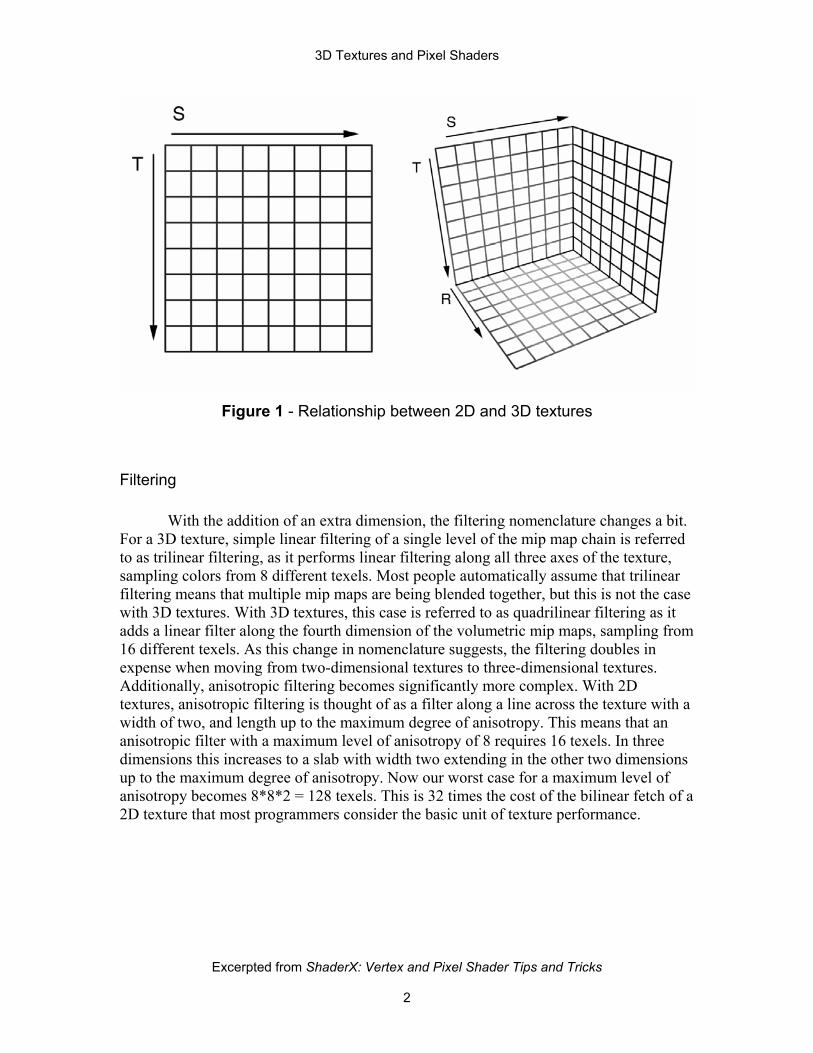
3D Textures Since 3D textures have appeared relatively recently in consumer-level hardware, many people are unfamiliar with exactly what they are. The simplest way to think of a 3D texture is as a stack of 2D textures. There are multiple conventions for referring to the coordinates used to index a 3D texture, for this chapter we will use s, t, r, and q. These are the width, height, depth, and projective coordinates respectively. This is different from the terminology used in DirectX documentation, but it avoids confusion as to whether w is the depth component or the projective component of a texture.
Excerpted from ShaderX: Vertex and Pixel Shader Tips and Tricks
1
3D Textures and Pixel Shaders
Figure 1 - Relationship between 2D and 3D textures
Filtering With the addition of an extra dimension, the filtering nomenclature changes a bit. For a 3D texture, simple linear filtering of a single level of the mip map chain is referred to as trilinear filtering, as it performs linear filtering along all three axes of the texture, sampling colors from 8 different texels. Most people automatically assume that trilinear filtering means that multiple mip maps are being blended together, but this is not the case with 3D textures. With 3D textures, this case is referred to as quadrilinear filtering as it adds a linear filter along the fourth dimension of the volumetric mip maps, sampling from 16 different texels. As this change in nomenclature suggests, the filtering doubles in expense when moving from two-dimensional textures to three-dimensional textures. Additionally, anisotropic filtering becomes significantly more complex. With 2D textures, anisotropic filtering is thought of as a filter along a line across the texture with a width of two, and length up to the maximum degree of anisotropy. This means that an anisotropic filter with a maximum level of anisotropy of 8 requires 16 texels. In three dimensions this increases to a slab with width two extending in the other two dimensions up to the maximum degree of anisotropy. Now our worst case for a maximum level of anisotropy becomes 8*8*2 = 128 texels. This is 32 times the cost of the bilinear fetch of a 2D texture that most programmers consider the basic unit of texture performance.
Excerpted from ShaderX: Vertex and Pixel Shader Tips and Tricks
2
3D Textures and Pixel Shaders
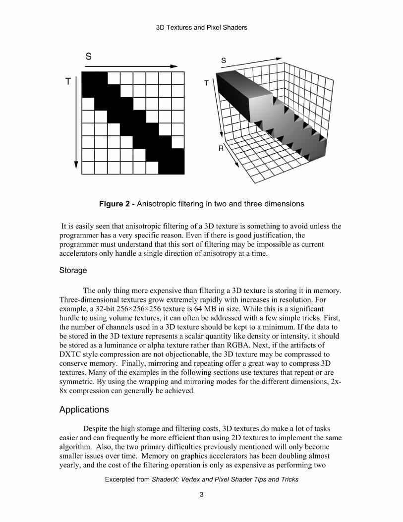
Figure 2 - Anisotropic filtering in two and three dimensions
It is easily seen that anisotropic filtering of a 3D texture is something to avoid unless the programmer has a very specific reason. Even if there is good justification, the programmer must understand that this sort of filtering may be impossible as current accelerators only handle a single direction of anisotropy at a time.
Storage The only thing more expensive than filtering a 3D texture is storing it in memory. Three-dimensional textures grow extremely rapidly with increases in resolution. For example, a 32-bit 256×256×256 texture is 64 MB in size. While this is a significant hurdle to using volume textures, it can often be addressed with a few simple tricks. First, the number of channels used in a 3D texture should be kept to a minimum. If the data to be stored in the 3D texture represents a scalar quantity like density or intensity, it should be stored as a luminance or alpha texture rather than RGBA. Next, if the artifacts of DXTC style compression are not objectionable, the 3D texture may be compressed to conserve memory. Finally, mirroring and repeating offer a great way to compress 3D textures. Many of the examples in the following sections use textures that repeat or are symmetric. By using the wrapping and mirroring modes for the different dimensions, 2x-8x compression can generally be achieved. Applications
Despite the high storage and filtering costs, 3D textures do make a lot of tasks easier and can frequently be more efficient than using 2D textures to implement the same algorithm. Also, the two primary difficulties previously mentioned will only become smaller issues over time. Memory on graphics accelerators has been doubling almost yearly, and the cost of the filtering operation is only as expensive as performing two
Excerpted from ShaderX: Vertex and Pixel Shader Tips and Tricks
3
3D Textures and Pixel Shaders
texture fetches of the same quality. Modern cards that support 1.4 pixel shaders are capable of performing up to twelve 2D fetches (which can each be trilinear, anisotropic etc) in a single pass.
Function of 3 independent variables The first and most obvious application for 3D textures in shaders is as look-up tables to provide piece-wise linear approximations to arbitrary functions of three variables. Many of the following sections show specific examples of functions of three dimensions, but it is important to remember the general concept rather than particular examples. One simple example would be an implementation of the per-pixel calculation of Phong style specular highlights. Since the half-angle (H) and reflection (R) vectors don’t interpolate linearly across the surface of polygons, they must be recomputed per-pixel to obtain the best results. This leads to the creation of a vector of non-unit length as graphics hardware is not yet able to perform a per-pixel square root. Naturally, the equation for specular highlights requires its inputs to be of unit length. The problem is that L · R or N · H, whichever you prefer, now is not just cos(θ), but is instead cos(θ) * |R| or cos(θ) * |H|. Clearly, this problem can be corrected by performing a normalizing divide prior to raising cos(θ) to the k’th power. Now, the function that needs to be evaluated is one of three variables: {N · H (cos(θ) * |H|), |H|, k} or {R · L (cos(θ) * |R|), |R|, k}. The equation actually implemented is shown below. The most important item to note about this particular algorithm is that it can be implemented much more efficiently as a projected 2D texture since the first operation is just a divide, but this example is good for illustrative purposes. General Equation
k
HHHN
⋅o where N H = 0 if N·H < 0 o
Pixel Shader
ps.1.4 texld r0.rgb, t0.xyz //get normal from a texture lookup texld r1.rgb, t1.xyz //get light vector in same way texld r2.rgb, t2.xyz //get view vector in same way texcrd r3.rgb, t3.xyz //pass in spec power in t3.x //compute H as V+L/2 add_d2 r1.rgb, r1_bx2, r2_bx2 //compute N.H and store in r0.r dot3 r0.r, r0_bx2, r1 //compute H.H and store in r0.g dot3 r0.g, r1, r1
Excerpted from ShaderX: Vertex and Pixel Shader Tips and Tricks
4
3D Textures and Pixel Shaders
//copy in k mov r0.b, r3.r phase texld r3, r0.rgb //fetch the 3D texture to compute specular //move it to the output mov_sat r0, r3
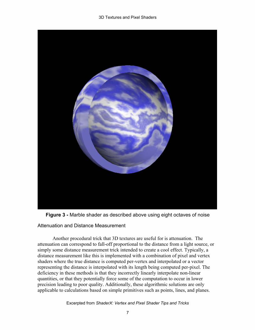
Noise and procedural texturing Noise is a particular type of function texture that is extremely useful in pixel shading. The noise that is most interesting to us here is not white noise of random numbers, but is instead Perlin noise that has smoothly varying characteristics [Perlin85]. Noise of this sort has been used for years in production quality 3D graphics for texture synthesis. It allows the creation of non-repeating fractal patterns like those found in wood, marble, or granite. This is especially interesting in that an effectively infinite texture can be created from finite texture memory. The most classic example for using a 3D noise function is to create turbulence. Turbulence is an accumulation of multiple levels (octaves) of noise for the purpose of representing a turbulent flow. A great example of this is the appearance of marble. The veins flow through the material in a turbulent manner. The example we will use is an adaptation for real-time of the Blue Marble shader from The RenderMan Companion [Upstill89]. In this example, the shader uses six textures to create the effect. The textures are five occurrences of a noise map and a one-dimensional color table. (Note that this shader will work even better with more noise textures—six is just the limit for DirectX 8.1’s 1.4 pixel shaders.) The noise textures are scaled and summed to create the turbulence and the value of the turbulence is then used to index a 1D texture via a dependent read to map it to a color. The texture coordinates used to index into the noise maps are all procedurally generated in the same manner, and they are just different scales of each other. Pixel Shader Code
ps.1.4 //fetch noise maps texld r0, t0.xyz texld r1, t1.xyz texld r2, t2.xyz texld r3, t3.xyz texld r4, t4.xyz //accumulate multiple octaves of noise
Excerpted from ShaderX: Vertex and Pixel Shader Tips and Tricks
5
3D Textures and Pixel Shaders
// this sets r0 equal to: // 1/2r0 + 1/4r1 + 1/8r2 + 1/16r3 + 1/32r4 add_d2 r3, r3_x2, r4 add_d2 r3, r2_x2, r3 add_d2 r3, r1_x2, r3 add_d4 r0, r0_x2, r3 phase //fetch 1-D texture to remap texld r5, r0.xyz mov r0, r5
Realistically, the interactive 3D graphics field is just now on the edge of getting procedural noise textures to work. Noise textures tend to require several octaves of noise, and dependent fetches just to implement something as simple as marble. This ignores the application of lighting and other effects one would also need to compute in the shader. As a result, it would be impractical to ship a game which relied upon noise textures of this sort today, but it still certainly applies as a technique to add that little bit of extra varying detail to help eliminate the repetitive look in many of today’s interactive 3D applications. Finally, even if this technique is not immediately applicable, graphics hardware is evolving at such a pace that we expect this technique will be very common in a few years.
Excerpted from ShaderX: Vertex and Pixel Shader Tips and Tricks
6
3D Textures and Pixel Shaders
Figure 3 - Marble shader as described above using eight octaves of noise
Attenuation and Distance Measurement Another procedural trick that 3D textures are useful for is attenuation. The attenuation can correspond to fall-off proportional to the distance from a light source, or simply some distance measurement trick intended to create a cool effect. Typically, a distance measurement like this is implemented with a combination of pixel and vertex shaders where the true distance is computed per-vertex and interpolated or a vector representing the distance is interpolated with its length being computed per-pixel. The deficiency in these methods is that they incorrectly linearly interpolate non-linear quantities, or that they potentially force some of the computation to occur in lower precision leading to poor quality. Additionally, these algorithmic solutions are only applicable to calculations based on simple primitives such as points, lines, and planes.
Excerpted from ShaderX: Vertex and Pixel Shader Tips and Tricks
7
3D Textures and Pixel Shaders
By using a 3D texture, the programmer is effectively embedding the object in a distance or attenuation field. Each element in the field can have arbitrary complexity in its computation since it is generated off-line. This allows the field to represent a distance from an arbitrary shape. On the downside, using a 3D texture can be reasonably expensive from a memory standpoint, and it relies on a piecewise linear approximation to the function from the filtering. The toughest portion of using a 3D texture to perform this sort of operation is defining the space used to for the texture and the transform necessary to get the object into the space. Below is a general outline of the algorithm:
1. Define a texture space containing the area of interest 2. For each texel in the space compute the attenuation 3. Apply the 3D attenuation texture to the object with appropriate texture
coordinate generation
The first step involves analyzing the data and understanding its symmetry and extents. If the data is symmetric along one of its axes, then one of the mirrored texturing modes, such as D3DTADDRESS_MIRRORONCE, can be used to double the resolution (per axis of symmetry) for a given amount of data. Additionally, an understanding of the extents of the data is necessary to optimally utilize the texture memory. If a function falls to a steady-state such as zero along an axis, then the texture address mode can be sent to clamp to represent that portion of the data. Once the user has fit the data into a space that is efficient at representing the function, the function must be calculated for each texel. Below is a pair of pseudocode examples showing how to fill an attenuation field for a point. The first is naïve and computes all the attenuation values in the shape of a sphere; the second takes advantage of the symmetry of the sphere and only computes one octant. This can be done as the values all mirror against any plane through the center of the volume.
Complete Sphere: #define VOLUME_SIZE 32 unsigned char volume[VOLUME_SIZE][VOLUME_SIZE][VOLUME_SIZE]; float x, y, z; float dist; //walk the volume filling in the attenuation function, // where the center is considered (0,0,0) and the // edges of the volume are one unit away in parametric // space (volume ranges from –1 to 1 in all dimensions x = -1.0f + 1.0f/32.0f; //sample at texel center for (int ii=0; ii<VOLUME_SIZE; ii++, x += 1.0f/16.0f) { y = -1.0f + 1.0f/32.0f; for (int jj=0; jj<VOLUME_SIZE; jj++, y += 1.0f/16.0f) { z = -1.0f + 1.0f/32.0f; for (int kk=0; kk<VOLUME_SIZE; kk++, y += 1.0f/16.0f) { //compute distance squared
Excerpted from ShaderX: Vertex and Pixel Shader Tips and Tricks
8
3D Textures and Pixel Shaders
dist = x*x + y*y + z*z; //compute the falloff and put it into the volume if (dist > 1.0f) { //outside the cutoff volume[ii][jj][kk] = 0; } else { //inside the cutoff volume[ii][jj][kk] = (unsigned char) ( 255.0f * (1.0f – dist)); } } } }
Sphere Octant, used with the D3DTADDRESS_MIRRORONCE texture address mode: #define VOLUME_SIZE 16 unsigned char volume[VOLUME_SIZE][VOLUME_SIZE][VOLUME_SIZE]; float x, y, z; float dist; //walk the volume filling in the attenuation function, // where the center of the volume is really (0,0,0) in // texture space. x = 1.0f/32.0f; for (int ii=0; ii<VOLUME_SIZE; ii++, x += 1.0f/16.0f) { y = 1.0f/32.0f; for (int jj=0; jj<VOLUME_SIZE; jj++, y += 1.0f/16.0f) { z = 1.0f/32.0f; for (int kk=0; kk<VOLUME_SIZE; kk++, y += 1.0f/16.0f) { //compute distance squared dist = x*x + y*y + z*z; //compute the falloff and put it into the volume if (dist > 1.0f) { //outside the cutoff volume[ii][jj][kk] = 0; } else { //inside the cutoff volume[ii][jj][kk] = (unsigned char) ( 255.0f * (1.0f – dist)); } } } }
Excerpted from ShaderX: Vertex and Pixel Shader Tips and Tricks
9
3D Textures and Pixel Shaders
With the volume, the next step is to generate the coordinates in the space of the texture. This can be done with either a vertex shader or the texture transforms available in the fixed-function vertex processing. The basic algorithm involves two transformations. The first translates the coordinate space to be centered at the volume, rotates it to be properly aligned, then scales it such that the area effected by the volume falls into a cube ranging –1 to 1. The second transformation is dependent on the symmetry being exploited. In the case of the sphere octant, no additional transformation is needed. With the full sphere, the transformation needs to map the entire –1 to 1 range to the 0 to 1 range of the texture. This is done by scaling the coordinates by one half and translates them by one half. All these transformations can be concatenated into a single matrix for efficiency. The only operation left to perform is the application of the distance or attenuation to the calculations being performed in the pixel shader.
Representation of amorphous volume One of the original uses for 3D textures was in the visualization of scientific and medical data [Drebin88]. Direct volume visualization of 3D datasets using 2D textures has been in use for some time, but it requires three sets of textures, one for each of the axes of the data and is unable to address filtering between slices without the use of multitexture. With 3D textures, a single texture can directly represent the data set. Although this chapter does not focus on scientific visualization, the implementation of this technique is useful in creating and debugging other effects using volume textures. Using this technique borrowed from medical volume visualization is invaluable in debugging the code which a developer might use to generate a 3D distance attenuation texture, for example. It allows the volume to be inspected for correctness, and the importance of this should not be underestimated, as presently an art tool for creating and manipulating volumes does not exist. Additionally, this topic is of great interest as a large amount of research is presently on-going in the area of using pixel shaders to improve volume rendering.
Application These general algorithms and techniques for 3D textures are great, but the really interesting part is the concrete applications. The following sections will discuss a couple applications of the techniques described previously in this chapter. They range from potentially interesting spot effects to general improvements on local illumination.
Volumetric fog and other atmospherics One of the first problems that jumps into many programmers’ minds as candidate for volume texture is the rendering of more complex atmospherics. So far, no one has been able to get good variable density fog and smoke wafting through a scene, but many have thought of volume textures as a potential solution. The reality is that many of the
Excerpted from ShaderX: Vertex and Pixel Shader Tips and Tricks
10
3D Textures and Pixel Shaders
rendering techniques that can produce the images at a good quality level just burn enormous mounts of fill-rate. Imagine having to render an extra fifty to one hundred passes over the majority of a 1024 x 768 screen to produce a nice fog effect. This just is not going to happen quite yet. Naturally, hardware is accelerating its capabilities toward this sort of goal, and with the addition of a few recently discovered improvements, this sort of effect might be acceptable. The basic algorithm driving the rendering of the atmospherics is based off the volume visualization shaders discussed earlier. The primary change is an optimization technique presented at the SIGGRAPH/Eurographics Workshop on Graphics Hardware in 2001 by Klaus Engel. The idea is that the accumulation of slices of the texture map is attempting to perform an integration operation. To speed the process up, the volume can be instead rendered in slabs. By having each slice sample the volume twice (at the front and rear of the slab), the algorithm approximates an integral as if the density varied linearly between those two values. This results in the slice taking the place of several slices with the same quality. The first step in the algorithm is to draw the scene as normal, filling in the color values that the fog will attenuate, and the depth values that will clip the slices appropriately. When rendering something like fog that covers most of the view, this means generating full-screen quads from the present viewpoint. The quads must be rendered back to front to allow proper compositing using the alpha blender. The downside to the algorithm is in the coarseness of the planes intersecting with the scene. This will lead to the last section of fog before a surface to be dropped out. In general, this algorithm is best for a fog volume with relatively little detail, but that tends to be true of most fog volumes.
Light falloff A more attainable application of 3D textures and shaders on today’s hardware is volumetric light attenuation. In its simplest form, this becomes the standard light-map algorithm everyone knows. In more complex forms, it allows the implementation of per-pixel lighting derived from something as arbitrary as a fluorescent tube or a light saber. In the simple cases, the idea is to simply use the 3D texture as a ball of light that is modulated with the base environment to provide a simple lighting effect. Uses for this include the classic rocket flying down the dark hallway to kill some ugly monster shader. Ideally, that rocket should emit light from the flame. The light should roughly deteriorate as a sphere centered around the flame. This obviously over-simplifies the real lighting one might like to do, but it is likely to be much better than the projected flashes everyone is used to currently. Implementing this sort of lighting falloff is extremely simple; one only needs to create a coordinate frame centered around the source of the illumination and map texture coordinates from it. In practice, this means generating texture coordinates from world or eye-space locations and back transforming them into this light-centered volume. The texture is then applied via modulation with the base texture. The
Excerpted from ShaderX: Vertex and Pixel Shader Tips and Tricks
11
3D Textures and Pixel Shaders
wrap modes for the light map texture should be set as described in the earlier section on the general concept of attenuation. Extending the simple glow technique to more advanced local lighting models brings in more complex shader operations. A simple lighting case that might spring to mind is to use this to implement a point light. This is not really a good use of this technique, as a point light needs to interpolate its light vector anyway to perform any of the standard lighting models. Once the light vector is available, the shader is only a dot product and a dependent texture fetch away from computing an arbitrary falloff function from that point. A more interesting example is to use a more complex light shape such as a fluorescent tube. The light vector cannot be interpolated between vertices, so a different method needs to be found. Luckily, a 3D texture provides a great way to encode light vector and falloff data. The light vector can be encoded in the RGB channels, and the attenuation can simply fit into the alpha channel. Once the correct texel is fetched, the pixel shader must rotate the light vector from texture space to tangent space by performing three dot products. Finally, lighting can proceed as usual. This algorithm uses the same logic for texture coordinate generation as the attenuation technique described earlier. The only real difference with respect to the application of the volume texture is that the light vector mentioned above in encoded in the texture in addition to the attenuation factor. The application of the light is computed in the following shader using the light vector encoded in the volume:
ps.1.4 texld r0.rgba, t0.xyz //sample the volume map texld r1.rgb, t1.xyz //sample the normal map texcrd r2.rgb, t2.xyz //pass in row 0 of a rotation texcrd r3.rgb, t3.xyz //pass in row 1 of a rotation texcrd r4.rgb, t4.xyz //pass in row 2 of a rotation //rotate Light vector into tangent space dot3 r5.r, r0_bx2, r2 dot3 r5.g, r0_bx2, r3 dot3 r5.b, r0_bx2, r4 //compute N.L and store in r0 dot3_sat r0.rgb, r5, r1_bx2 //apply the attenuation mul r0.rgb, r0, r0.a
The only tricky portion of this shader is the rotation into tangent space. The rotation matrix is stored in texture coordinate sets two through four. This matrix must rotate from texture space to surface space. This matrix is generated by concatenating the matrix composed of the tangent, binormal, and normal vectors (the one typically used in per-pixel lighting) with a matrix to rotate the texture-space light vector into object space.
Excerpted from ShaderX: Vertex and Pixel Shader Tips and Tricks
12
3D Textures and Pixel Shaders
Excerpted from ShaderX: Vertex and Pixel Shader Tips and Tricks
13
This matrix can easily be derived from the matrix used to transform object coordinates into texture space. References [Drebin88] Robert A. Drebin, Loren Carpenter and Pat Hanrahan, “Volume Rendering”, ACM SIGGRAPH Computer Graphics, Vol.22, No. 4, August 1988, pp 65-74. [Upstill89] Steve Upstill, The RenderMan Companion, Addison Wesley. [Perlin85] Ken Perlin, “An Image Synthesizer”, ACM SIGGRAPH Computer Graphics, Vol. 19, No. 3, July 1985, pp 287-296