Pricing the Razor: Evidence on two-part tariffs

Zheng Yang ∗

Department of Economics, University of Kentucky

October 26, 2018

Abstract

This paper finds evidence from men’s razor market for the hypothesis that tie-in

sale can be used to implement a two-part tariff pricing strategy. I estimate a demand

system of the razor by random coefficient logit model with market level sales data from

Nielsen Store Scanner dataset and individual demographics data from March CPS.

The estimated parameters are used to construct price-cost markup. By comparing the

markups of different products, I find the evidence that Gillette is using two-part tariff

strategy. This conclusion can be generalized as that a monopolist can set the prices of

tie-in products in line with two-part tariff.

∗E-mail: zheng.yang@uky.eduThis paper is part of my dissertation. Please do not cite or circulate without the author’s permission.

Researcher(s) own analyses calculated (or derived) based in part on data from The Nielsen Company (US),LLC and marketing databases provided through the Nielsen Datasets at the Kilts Center for Marketing DataCenter at The University of Chicago Booth School of Business.

The conclusions drawn from the Nielsen data are those of the researcher(s) and do not reflect the viewsof Nielsen. Nielsen is not responsible for, had no role in, and was not involved in analyzing and preparingthe results reported herein.

1

1 Introduction

In this paper, the hypothesis that tie-in sale can be used as two-part tariff method

is confirmed by evidence from men’s razor market. I estimate a random coefficient

logit model with the market level razor sales data in the United States between 2015

to 2016. The estimated parameters are used to compute the price-cost markup of

each product. Then I compare the markups of different products. The result shows

that Gillette charged high markups to its disposable razors and low markups to its

cartridges. Further, the markup difference contributes to most of the price difference.

Last, the markup difference of Gillette’s brands is more significant than that of a fringe

competitor. This result is explained as that Gillette intentionally lowers down cartridge

price to promote sales when it can use the handle to extract consumers surplus from

shave services. In other words, the tie-in nature of men’s non-disposable razor system

is used to implement a two-part tariff pricing strategy.

When a service is provided jointly by a durable foremarket good and a non-durable

aftermarket good, a firm can force the foremarket good buyers to buy its aftermarket

good by tie-in arrangement or compatibility. This business strategy is called tie-in

sale.1 Examples of tie-in sales include printer and inks, video game console and games,

and razor handle and cartridges. An interesting problem regarding to tie-in sale is

what is the best pricing schedule of foremarket good and aftermarket good.

A common view, usually referred as “razor-and-blades” business model, says that

a firm should set a low price on foremarket good or even give it away and set a high

price on aftermarket good. Due to the low foremarket price, more consumers buy that

foremarket product and are locked with this firm. Then the firm can set a high price

on aftermarket good. The “razor-and-blades” model reveals the coordination between

pricing on two products. However, it is doubtful that the “razor-and-blades” pricing

strategy applies to all tie-in products, especially to razors.

1There are different definitions of “tie-in sale”. For example, “bundling” (selling one product with a fixednumber of another product) is sometimes called “tie-in sale”. Also, as Burnstein 1960 says, tie-in productsare not necessarily complementary. In this paper, I use a narrow definition of “tie-in sale”.

2

Picker (2011) raises a critical view regarding the “razor-and-blades” story. He traces

back the razor prices in the early 20th century with some historical evidence, such as

the advertisements in magazines. It turns out that the Gillette company charged $5

for a razor handle with a pack of 12 cartridges and $1 for each additional pack of 12

cartridges when it monopolized this market with the patents from 1904 to 1921. After

its patents expired, Gillette lowered the price of the original handle set to $ one but

offered a new, luxury, but compatible handle set at $5. On the contrary, the price of

cartridges did not change over time. Picker concludes that Gillette was not playing

“razor-and-blades” strategy during its monopoly time until it was being challenged by

entrants.

The strategy Gillette played might be two-part tariff. This pricing strategy, which

is firstly analyzed by Oi (1971), involves setting a low marginal price for a service and

extracting the consumer surplus by charging a high lump-sum fee. Schmalensee (1981,

2015) says that the two-part tariff can take the form of a tie-in sale; that is, a cartridge

provides unit shave service while the handle price can be viewed as a lump-sum fee.

According to this theory, a monopolistic razor company sells the handles at a high

price and the cartridges at a low price. Facing a low cartridge price, a consumer would

like to replace it more frequently. As his cartridge consumption increase, his willingness

to pay for the razor handle also go up. Thus, the consumer can readily accept a high

handle price. For the firm, a high handle price can not only compensate for the loss

caused by lowering the cartridge price but also extract more consumer surplus.

The main difference between the “razor-and-blade” story and the “two-part tariff”

theory arises from their assumptions about market structure. There are two separated

but interdependent market: the handle market and the cartridge market. The “razor-

and-blades” story implicitly assumes that the handle market is a competitive market.

Thus, each razor company would like to lower its razor price to compete with each

other. However, if a consumer has bought a handle, he is locked to the cartridges of

the same brand. Thus, each company is a local monopolist in the cartridge market and

can set a high cartridge price. On the contrary, the “two-part tariff” theory assumes

3

that a razor company is a monopolist in both the handle and the cartridge markets.

Even if being charged a high handle price, the consumers would not switch to other

brands.

When monopolizing this market (1904 – 1921), Gillette did not need to lower its

handle price to compete with anyone. So, it was feasible to two-part tariff strategy

during its monopoly period. But, when its patent was expired, Gillette had to lower

down the handle price to compete with other firms. However, when the price of a

handle was not high enough, a consumer may not care about the switching cost; that

is, purchasing a new handle from other company. Thus, the handle could not lock the

consumers. In other words, giving handles away could not help the companies raise

the prices in the cartridge market.

Picker’s evidence is not thorough enough. Gillette did set a high handle price and

a relatively low cartridge price during the monopolistic period. However, it is unclear

that what the costs of the handle and the cartridge were. It is possible that the cost

made up a high percentage of the handle price but a low percentage of the cartridge

price. In this case, even a high handle price and low cartridge price could be a “razor-

and-blades” price strategy. Also, it is still unclear that what pricing strategy Gillette

is using nowadays.

To my knowledge, this is the first paper to examine tie-in sales as a two-part

tariff. There is a growing body of literature regarding pricing on tie-in products.

Li (2015) studies the optimal intertemporal price discrimination schedule in the e-

reader and e-books industry. She finds the optimal pricing schedule depends on use

intensity. For avid consumers, a firm should harvest (price-cutting over time) on e-

readers and investing (price-raising over time) in e-books. For general consumers,

a firm should invest in e-readers and harvest on e-books. Chintagunta, Qin, and

Vitorino (2018) investigate single-serve coffee system industry, where coffee machine

manufacturer licenses other firms to produce coffee pods. They find licensing agreement

is associated with less price dispersion in the afermarket and lower prices of primary

good. Gil and Hartman (2009) and Hartmann and Nair (2010)’s findings are more close

4

to this paper. Gil and Hartman study the concession sales at movie theaters. They

find the demand condition for movie tickets and concession supports metering strategy

(setting a low price for movie tickets and high price for concession). They also find high-

priced concessions do extract more surplus from customers with a greater willingness

to pay for the tickets. Hartmann and Nair (2010) find the demand condition in men’s

razor market is feasible for the two-tariff strategy (setting a high price for handles and

low price for cartridges). However, these papers only show that when pricing tie-in

products what the firms should do, rather than what they did.

According to identifying which pricing strategy is actually used by firms, Shepard

(1991) reveal evidence that gas stations use a quality scale to discriminating consumers.

The price difference of full-service gasoline between a multi-product gas station (pro-

viding both full-service gasoline and self-service gasoline) and a single product gas

station (only providing self-service gasoline) is driven by price discrimination. Ver-

boven (1996, 2002) and Cohen (2008) find that the price difference across consumer

groups can be explained by markup difference, which is evidence of price discrimina-

tion. Lakdawalla and Sood (2013) compare the difference in drug consumptions of

insured and uninsured patients across markets. They find the health insurance works

as a two-part tariff arrangement. Bonnet and Dubois (2010) study the bottled water

wholesale market and find evidence that there exists a two-part arrangement between

manufacturers and retailers.

This paper contributes the existing literature in two aspects. First, it provides

evidence to correct a common misunderstanding regarding the pricing strategy upon

razors. More generally, this paper confirms that tie-in sale can be used to play a two-

part tariff strategy. Moreover, this paper enriches the empirical literature of pricing

on tie-in sales, price discrimination, and application of random coefficient logit model

on pricing.

The rest of this paper proceeds as follows. Section II presents a brief description

of the men’s shaving razor market. Section III presents the theoretical model of firm

pricing behavior. Section IV discusses the empirical strategy. Section V introduces

5

the data and the variables. Section VI presents the empirical results. And section VII

presents the conclusion.

2 Men’s shaving razor market

This section presents a brief introduction of men’s razor market. Section 2.1 will

introduce the product differentiation and heterogeneous consumers. The nature of

the products and consumer preference calls for using random coefficient logit model

when estimating demand system. Section 2.2 will introduce the market structure. We

will find that Gillette dominates the high-end segment of this market and other firms

are fringe competitors. Thus, Gillette can implement two-part pricing in this market

segment while other firms may not be able to do that. Section 2.3 presents some

stylized facts regarding pricing strategy in the high-end segment.

2.1 Products and Demand

There are over two hundred highly differentiated brands in the men’s shaving razor

market. The main quality difference among them is the number of blades built in a

razor head, which ranges from one to six. The manufacturers claim that the more

blades a razor has, the more comfortable the shave is. Compared with the count of

blades, other quality differences are harder to observe or measure by the researchers.

For example, some brands have finer blades than the others. However, it is hard to

measure the sharpness of a blade. Also, the perceived quality is affected by advertising.

For example, by advertising, Gillette successfully sets its products apart from the other

brands. However, it is hard to find a valid measurement for the advertisement.

The brands are also differentiated horizontally. For example, Sensor 3 and Mach 3

are different brands sold by Gillette. However, there is no significant quality difference

between them. Both of them have three blades, a built-in trimmer, and a lubrication

stripe. It is likely that the main differences are the name and packaging design.

Another horizontal difference which this paper concerns about is the category; that

6

is, disposable or non-disposable. A disposable razor is a razor head attached with a

handle. The handle is not durable and would be discarded with the razor head. A

non-disposable system consists of a well-made handle with the replaceable cartridges.

A user of the non-disposable system can keep the handle for a long while and only

replace the cartridge in the short term.

The average quality of the non-disposable brands is higher than that of the dispos-

able brands. However, it does not mean that a non-disposable system is superior to

a disposable razor. Some brands, such as Gillette’s Mach 3 and Fusion, offers both

disposable razor and non-disposable system, which have the same razor head. Since

the consumers care more about the razor head rather than the handle, they might be

indifferent between a disposable razor and a non-disposable system.

The consumers have a variety of preference according to those product characteris-

tics. Further, ethnicity, age, and income affect the preference profoundly. For example,

Mintel’s research2 says that the low-income group is partial to the disposable razors

and a Hispanic is more likely to buy a high-quality razor. Since demographics make-

ups vary across areas and change over time, we can witness distinctive preferences in

markets.

2.2 Market Structure

Men’s shaving razor market is highly concentrated. From 2015 through 2016, the

top three companies, Gillette, Schick, and BiC, contributed 64.1% of the total sales

volume. Gillette, the dominator, attained 39.0% of the total sales volume, while Schick

and BiC acquired 10.7% and 14.4% respectively. As it has been mentioned above,

the count of blades is the main quality factor. Thus, the market can be split into

two segments by quality. The high-end segment consists of the razors with five or six

blades, while the low-end segment contains the razors with no more than four blades.

The low-end segment is more competitive. Gillette only attained 34.5% sales vol-

2Mintel is a privately owned market search firm whose databases and analysis are accessible to universitystudents.

7

ume. Schick’s market share shrank to 10.1%. And BiC acquired 16.1% of this market.

A non-negligible force in this market segment are the private-label brands3, which as

a whole seized 35.9% of the low-quality segment. The private-label brands are often

priced lower than a main-stream brand. In other words, they are price-taker rather

than price-maker. Thus, they probably do not have any market power. However, if

the purchasers of the low-quality razors are more sensitive to price, then Gillette would

also lose its market power due to the existence of the private-label brands.

In contrast, the high-end market is monopolized by Gillette. Gillette made up to

58.1% of the advanced razors; that is almost four times its largest opponent’s market

share.

Table 1: Market Share

Overall Low-End High-End

Gillette 39.0 34.5 58.1

Schick 10.7 10.1 13.5

BiC 14.4 16.1 7.1

Private Label 31.6 35.9 13.2

Generic Brands 4.3 3.4 8.1

The competition also comes from outside. The established companies face increas-

ing challenge from online subscription service.4 Also, spas and salons offer professional

services to customers who prefer old school grooming. Boutique retailers sell luxury

shaving products to people who view shaving more of a ritual. Moreover, some con-

sumers prefer electric shavers. However, those competitors are not likely to affect the

market power of Gillette.

8

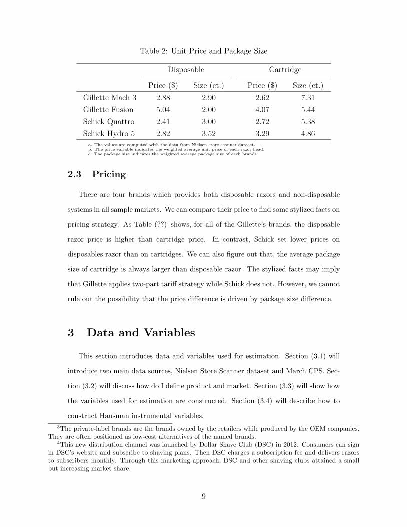
Table 2: Unit Price and Package Size

Disposable Cartridge

Price ($) Size (ct.) Price ($) Size (ct.)

Gillette Mach 3 2.88 2.90 2.62 7.31

Gillette Fusion 5.04 2.00 4.07 5.44

Schick Quattro 2.41 3.00 2.72 5.38

Schick Hydro 5 2.82 3.52 3.29 4.86a. The values are computed with the data from Nielsen store scanner dataset.b. The price variable indicates the weighted average unit price of each razor head.c. The package size indicates the weighted average package size of each brands.

2.3 Pricing

There are four brands which provides both disposable razors and non-disposable

systems in all sample markets. We can compare their price to find some stylized facts on

pricing strategy. As Table (??) shows, for all of the Gillette’s brands, the disposable

razor price is higher than cartridge price. In contrast, Schick set lower prices on

disposables razor than on cartridges. We can also figure out that, the average package

size of cartridge is always larger than disposable razor. The stylized facts may imply

that Gillette applies two-part tariff strategy while Schick does not. However, we cannot

rule out the possibility that the price difference is driven by package size difference.

3 Data and Variables

This section introduces data and variables used for estimation. Section (3.1) will

introduce two main data sources, Nielsen Store Scanner dataset and March CPS. Sec-

tion (3.2) will discuss how do I define product and market. Section (3.3) will show how

the variables used for estimation are constructed. Section (3.4) will describe how to

construct Hausman instrumental variables.

3The private-label brands are the brands owned by the retailers while produced by the OEM companies.They are often positioned as low-cost alternatives of the named brands.

4This new distribution channel was launched by Dollar Shave Club (DSC) in 2012. Consumers can signin DSC’s website and subscribe to shaving plans. Then DSC charges a subscription fee and delivers razorsto subscribers monthly. Through this marketing approach, DSC and other shaving clubs attained a smallbut increasing market share.

9

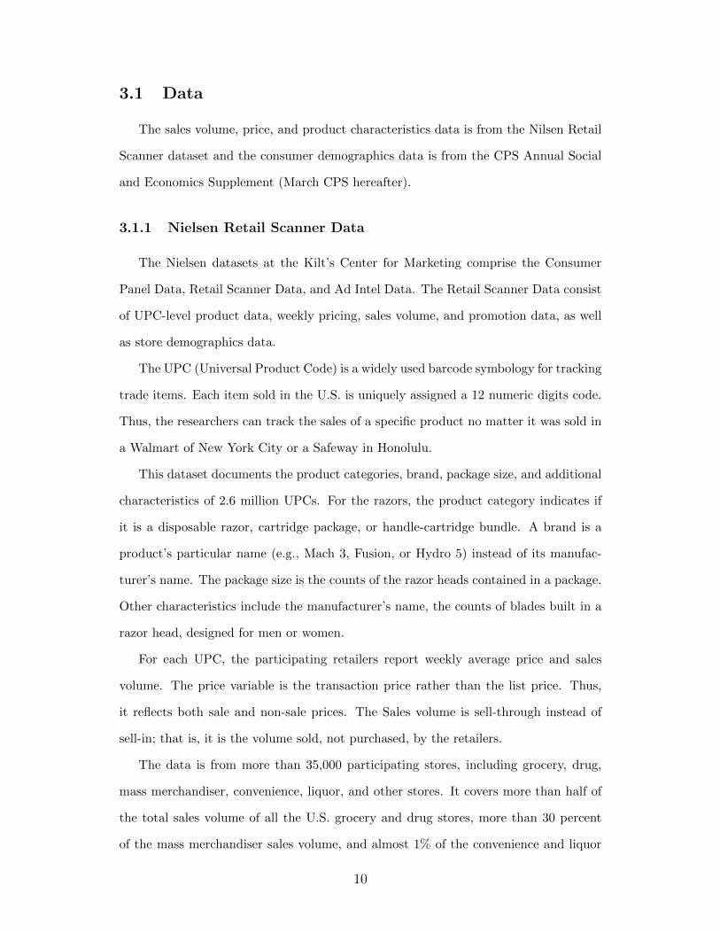
3.1 Data

The sales volume, price, and product characteristics data is from the Nilsen Retail

Scanner dataset and the consumer demographics data is from the CPS Annual Social

and Economics Supplement (March CPS hereafter).

3.1.1 Nielsen Retail Scanner Data

The Nielsen datasets at the Kilt’s Center for Marketing comprise the Consumer

Panel Data, Retail Scanner Data, and Ad Intel Data. The Retail Scanner Data consist

of UPC-level product data, weekly pricing, sales volume, and promotion data, as well

as store demographics data.

The UPC (Universal Product Code) is a widely used barcode symbology for tracking

trade items. Each item sold in the U.S. is uniquely assigned a 12 numeric digits code.

Thus, the researchers can track the sales of a specific product no matter it was sold in

a Walmart of New York City or a Safeway in Honolulu.

This dataset documents the product categories, brand, package size, and additional

characteristics of 2.6 million UPCs. For the razors, the product category indicates if

it is a disposable razor, cartridge package, or handle-cartridge bundle. A brand is a

product’s particular name (e.g., Mach 3, Fusion, or Hydro 5) instead of its manufac-

turer’s name. The package size is the counts of the razor heads contained in a package.

Other characteristics include the manufacturer’s name, the counts of blades built in a

razor head, designed for men or women.

For each UPC, the participating retailers report weekly average price and sales

volume. The price variable is the transaction price rather than the list price. Thus,

it reflects both sale and non-sale prices. The Sales volume is sell-through instead of

sell-in; that is, it is the volume sold, not purchased, by the retailers.

The data is from more than 35,000 participating stores, including grocery, drug,

mass merchandiser, convenience, liquor, and other stores. It covers more than half of

the total sales volume of all the U.S. grocery and drug stores, more than 30 percent

of the mass merchandiser sales volume, and almost 1% of the convenience and liquor

10

stores. Also, the coverage varies across the geographic markets. It ranges from 1%

to 86% for the grocery stores and from 28% to 92% for the drug stores. The data

is started with 2006 and updated annually. The updates lag by two years (e.g., 2016

Retail Scanner data was released in 2018).

The store demographics include store chain code, channel type, and area location.

The area location is indicated by FIPS code, which uniquely identifies in which county

or state a store locates.

3.1.2 March CPS

The March CPS is an annual survey conducted by the United States Census Bureau

for the Bureau of Labor Statistics. This data report the income received in the previous

calendar year, gender, race, age, and other demographics of each surveyed household or

individual. Over 90,000 households and 185,000 individuals are selected for producing

accurate estimates for the entire nation.

Also, the households and individuals are from 278 selected core-based statistical

areas (CBSA hereafter), 30 selected combined statistical areas, and 217 selected coun-

ties. The number of surveyed individuals varies across areas. For example, there are

10086 individuals from Los Angeles–Long Beach–Glendale of California, but only 100

individuals from Vineland–Bridgeton of New Jersey. The samples for the smaller areas

should be not wholly representative. Thus, the estimates for the smaller areas might

be invalid while the estimates for the larger areas should be more convincing. 5

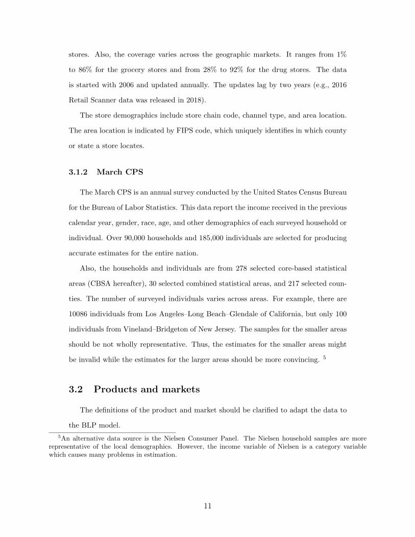
3.2 Products and markets

The definitions of the product and market should be clarified to adapt the data to

the BLP model.

5An alternative data source is the Nielsen Consumer Panel. The Nielsen household samples are morerepresentative of the local demographics. However, the income variable of Nielsen is a category variablewhich causes many problems in estimation.

11

3.2.1 Products

A product is defined by brand in conjunction with category (i.e., disposable or

cartridge). The packages of different size are treated as one product. Regarding this

definition, for example, Gillette’s Fusion disposable razor and cartridge are different

products. But a four-count package of Fusion cartridge is the same product as an eight-

count package. Store-owned brands and Generic brands are dropped. The generic

brands are excluded since none of them has more than 1% market share. On the

contrary, although the store-owned brands as a whole attains large market fraction,

each of them is only sold in certain outlets.6 All the singe-blade and twin-blade brands

are dropped for the reason that none of them offer both the disposable and cartridge.

And the quality difference between these disposables and cartridges is significant. Also,

local brands which do not cover all the geographic markets are excluded for simplicity.

Handle-cartridge bundles are dropped to make the data compatible with the de-

mand model. In the discrete choice model, each consumer is assumed to select one

product among numerous options. However, a consumer of the non-disposable system

is likely to buy both the cartridge package and the handle-cartridge bundle. Dropping

all non-disposable bundles is questionable. However, there are two reasons for what

this treatment is acceptable. First, the handle-cartridge bundles only attain 4.43% of

the volume sales. Thus, dropping it would not severely affect the empirical results. In

addition, the vast majority of the handle-cartridge bundles contain only one cartridge.

Thus, it is reasonable to assume that the consumers purchase handle-cartridge bundles

mainly for the handles and the handle-cartridge bundles are not competing with the

cartridges or disposable razors.

Under this context, the consumer choice set consists of 18 inside products (listed

in Table ??), which are manufactured by three companies (Gillette, Schick, and BiC),

and an outside product. The outside product can be a dropped product or a distant

6Another reason for what private label brand is excluded is that, since costs of private label brands ofdifferent retailers are different, so it is hard to find an instrumental variable for their prices to control forsimultaneity. A possible way to include private label is to define private label brands sold by different retailchains as different brands.

12

substitute such as an electric shaver or professional service in a salon. In other words,

the outside product represents the consumption of the potential consumers who did

not buy any inside products.

Table 3: Brands Used For Estimating Demand

3-Blade 4-Blade 5-Blade

Disposable:

G Custom Plus 3 S Quattro Titanium G Fusion

G Mach 3 B Flex 4 S Hydro 5

G Sensor 3

S Xtreme 3

B Comfort 3

B Comfort 3 Advance

B Flex 3

Cartridge:

G Mach 3 S Quattro Titanium G Fusion

G Mach 3 Turbo G Fusion ProGlide

S Hydro 3 S Hydro 5

Note: “G” represents Gillette, “S” as Schick, and “B” as BiC.

3.2.2 Markets

The market is defined by a geographic area in conjunction with a quarter. A

geographic area is a core-based statistical area (CBSA) which consists of an urban

center and adjacent counties that are socioeconomically tied to the urban center. Since

the small areas do not have representative March CPS samples, the areas which have

less than 40 male individuals in March CPS are dropped. Then, 77 geographic areas left

in the sample. Since the number of geographic areas is not large enough, observations

in different quarters are introduced to expand the sample size. The sample consists of

8 quarters, ranging from the first quarter of 2015 to the last quarter of 2016.

Figure: CBSAs in sample

13

There are 616 markets in total. And, in each of these markets, there are 18 products.

Then the sample consists of 11088 observations.

3.3 Variables

The variables used to estimate the BLP model consist of market share, price, pack-

age size, handle price (for cartridge), cartridge dummy, and brand dummies.

The market share of each inside product is as the ratio of sales volume to market

size.

The sales volume data of Nielsen Retail Scanner is UPC-store-weekly level. It is

aggregated to product-area-quarterly level for estimation.

As it has been mentioned above, the products of the same brand and category but

different package sizes (then different UPC) are treated as the same product in this

paper. Also, the manufacturers have been known to use more than one UPC for the

same product.7 Thus, it is reasonable to aggregate UPC-level data to the product-level.

Also, it is necessary to use the aggregated product definition. If there are too many

products in the consumers’ choice space, each of them should have a smaller market

share, which causes more problems due to the nature of the BLP model.

BLP model simulates the market share with the consumer demographics. It is hard

to know the consumer demographics of each store. But the consumer demographics in

an area is accessible. Thus, the store-level data is aggregated to the area-level.

Also, the sales volume data is hugely messy week-to-week. The sales volume can

change by more than fifty percent due to the promotion or other occurrences. Aggregat-

ing the weely-level data to quarterly-level reduces the effect of the random disturbances.

The market size of each area is measured by the maximum total sales volume of all

inside and outside products from 2013 through 2016. Thus, the market size differs in

the area but keeps constant over time.8

7They could offer a new package design to attract people who are open to change while keeping the olddesign for the conservative consumers.

8Cohen (2008) argues that this measurement may underestimate the real market size. As a result,estimated price elasticities would be smaller than the actual value. An alternative way is to assume that

14

The price variable is the weighted average unit price. It is calculated as the ratio of

total dollar sales to total sales count in a market. The denominator is the count of the

razor heads instead of the package. In other words, the price variable represents the

average price of each razor head rather than the package. The package size variable is

the weighted average package size. It is the ratio of total razor-head sold to total sales

volume. It has been known that a handle is sold with at least one cartridge, which

means there is no price data for the handles. The handle price is estimated by the

price of the handle-cartridge bundle with only one cartridge minus the unit price of

the cartridge of the same brand.

The product characteristics are captured by cartridge dummy, blade-count dum-

mies, and maker dummies. Instead of a category variable, two blade-count dummies

are used to measure the quality difference due to the blade-count difference. Also, the

maker dummies are used to identify if a product is produced by Gillette, Shick, or BiC.

According to Nevo (2000, 2001), the brand dummies are introduced to control for

those unobserved characteristics product characteristics which affect the consumers’

choice but cannot be observed or measured by economists. There are four brands

(Mach 3, Fusion, Quattro Titanium, Hydro 5) which offer both the disposable and

cartridge. Thus, unlike Nevo’s paper, the number of brand dummies does not equal

the number of products.

Also, 7 quarter dummies are used to control for the seasonal fix effect and the trend.

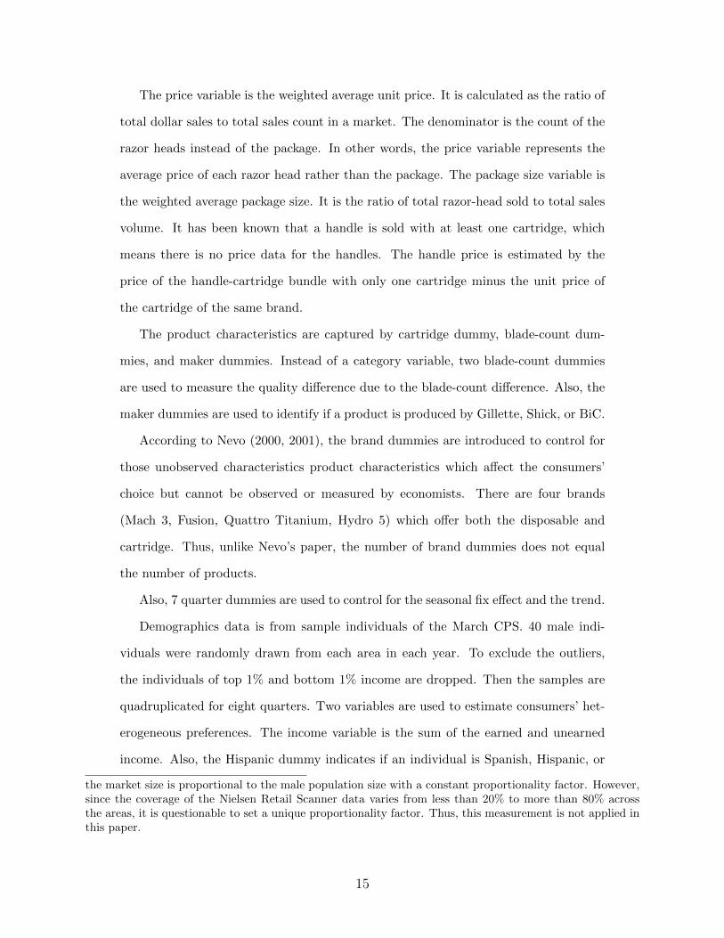
Demographics data is from sample individuals of the March CPS. 40 male indi-

viduals were randomly drawn from each area in each year. To exclude the outliers,

the individuals of top 1% and bottom 1% income are dropped. Then the samples are

quadruplicated for eight quarters. Two variables are used to estimate consumers’ het-

erogeneous preferences. The income variable is the sum of the earned and unearned

income. Also, the Hispanic dummy indicates if an individual is Spanish, Hispanic, or

the market size is proportional to the male population size with a constant proportionality factor. However,since the coverage of the Nielsen Retail Scanner data varies from less than 20% to more than 80% acrossthe areas, it is questionable to set a unique proportionality factor. Thus, this measurement is not applied inthis paper.

15

Latino.

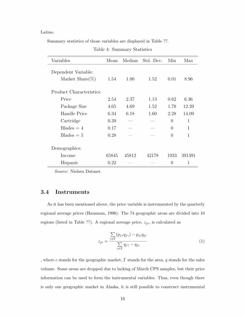
Summary statistics of those variables are displayed in Table ??.

Table 4: Summary Statistics

Variables Mean Median Std. Dev. Min Max

Dependent Variable:

Market Share(%) 1.54 1.00 1.52 0.01 8.96

Product Characteristics:

Price 2.54 2.37 1.13 0.62 6.36

Package Size 4.65 4.69 1.52 1.78 12.39

Handle Price 6.34 6.18 1.60 2.28 14.09

Cartridge 0.39 — — 0 1

Blades = 4 0.17 — — 0 1

Blades = 5 0.28 — — 0 1

Demographics:

Income 65845 45812 42178 1933 391391

Hispanic 0.22 — — 0 1

Source: Nielsen Dataset.

3.4 Instruments

As it has been mentioned above, the price variable is instrumented by the quarterly

regional average prices (Hausman, 1996). The 74 geographic areas are divided into 10

regions (listed in Table ??). A regional average price, zjc, is calculated as

zjc =

∑γ∈Γ

(pjγqjγ)− pjcqjc∑γ∈Γ

qjγ − qjc(1)

, where c stands for the geographic market, Γ stands for the area, q stands for the sales

volume. Some areas are dropped due to lacking of March CPS samples, but their price

information can be used to form the instrumental variables. Thus, even though there

is only one geographic market in Alaska, it is still possible to construct instrumental

16

variables for that area. The regional average prices of each quarter from 2014 Q1

through 2016 Q4 are used as instruments. Thus, there are 12 instruments for the price

variable.

Figure 1: Regions

Resources: www.wikimedia.org

4 Model

This section shows that, facing the same consumer demand, the optimal cartridge

price under two-part tariff is below that under linear pricing. And the latter one is

numerically equals to the price of a disposable razor. Also, if the disposable razors are

sold to low-demand consumers while cartridges are sold to high-demand consumers,

the cartridge price is below the disposable razor price.

4.1 A continuum model

Consider a market in which each consumer has a linear demand function for shaving

service, q = −αp+λ. Without loss of generality, suppose that α = 1 and λ is uniformly

distributed between 0 and 1. Then we get a continuous distribution of consumers whose

demand curves are parallel. Facing a two-part tariff, each consumer will choose the

17

quantity of cartridge at first, and then compare the consumer surplus he can get from

the cartridges with the price of a handle. If the consumer surplus exceeds the handle

price, then he will purchase both the handle and cartridges. Otherwise, he will not

purchase anything. In other words, the individual rationality condition is

1

2(λ− pc)2 −R ≥ 0 (2)

, where pc stands for the cartridge price and R stands for the handle price. Since

each consumer who stays in the market purchases one handle, the demand function of

handle is N = 1− λ, where λ stands for the marginal consumer.

A monopolist should maximize its profit from the cartridges and handles subject

to the consumers’ individual rationality condition; that is,

maxpc,R

∫ 1

λ(λ− pc)pcdλ+ (1− λ)R

s.t.1

2(λ− pc)2 −R ≥ 0 for any λ ∈ [λ, 1]

(3)

The marginal cost of handle and cartridge are assumed to be zero. By the individual

rationality condition, the marginal consumer is determined with

λ = pc +√

2R (4)

Solving equation (??) and use of (??) yield

p2PTc =

1

5

R2PT =2

25

(5)

Now suppose that, this monopolist does not use two-part tariff to price razor and

handle (or, say, this firm is using linear pricingstrategy). In other words, it sets the

price of cartridge first without taking cartridge sales into account, and then set handle

18

price as cartridge price is given. Then, this firm’s problem becomes

maxpc

∫ 1

λ(λ− pc)pcdλ (6)

and

maxR

(1− λ)R

s.t.1

2(λ− pc)2 ≥ R for any λ ∈ [λ, 1]

(7)

Solving for this problem yields the optimal price schedule

pLPc =1

3

RLP =8

81

(8)

Last, suppose this monopolist does not offer the non-disposable system, it sells

disposable razors as instead, then this firm’s problem becomes

maxpd,R

∫ 1

λ(λ− pd)pddλ

s.t.1

2(λ− pd)2 ≥ 0 for any λ ∈ [λ, 1]

(9)

, where pd stansd for price of a disposable razor. Solving for this problem yields

p∗d =1

3(10)

Equation (4), (7), and (10) establish that

Proposition 1: Serving the same demand, the cartridge price under two-part tariff is

above the cartridge price under linear pricing. The cartridge price under linear pricing

is numerically equal to the price of the disposable razor.

p2PTc < pLPc = pd (11)

19

The reason for what a monopolist charges a smaller markup for the cartridge is: when

a consumer buys the cartridges, he also need to buy a handle to get the shave service.

Thus, the monopolist earn profits from not only the cartridges but also the handle.

Further, if the monopolist lowers down the price of the cartridge, the buyer will consume

more. Then his consumer surplus from the cartridges and willingness to pay for the

handle goes up. And the monopolist can charge a higher price for the handle.

4.2 A two-type model

Now consider a market with two types of consumers whose demand functions for

shave are qL = λL−p and qH = λH −p, where λL < λH . A monopolist simultaneously

offers disposable razor or non-disposable system to each consumer. Also, this monop-

olist is implementing self-selection mechanism: the price scheme is designed to induce

high-demand consumers to buy the non-disposable system and low-demand consumers

to buy the disposable razor. In other words, the incentive compatibility conditions

must hold

1

2(λL − pd)2 ≥ 1

2(λL − pc)2 −R

1

2(λH − pc)2 −R ≥ 1

2(λH − pd)2

(12)

. The first equation means the low-demand consumers have no incentive to buy the

cartridges while the second equations means the high-demand consumers have no in-

centive to buy the disposable razors.

Now, the firm’s problem is

maxpd,pc,R

n(pd − cd)(λL − pd) + (1− n)(pc − cc)(λH − pc) + (1− n)R

s.t.1

2(λL − pd)2 ≥ 0

1

2(λH − pc)2 −R ≥ 0

1

2(λL − pd)2 ≥ 1

2(λL − pc)2 −R

1

2(λH − pc)2 −R ≥ 1

2(λH − pd)2

(13)

20

, where n stands for the fraction of the low-demand consumers. The first two constraints

are individual rationality conditions as in equation (??), while the last two are the

incentive compatibility conditions. Solving equation (??), we get the optimal pricing

scheme as

pd =n

1 + nλL +

1− n1 + n

λH +n

1 + ncd

pc = cc

R = (λH − cc)2 − (n

1 + n)2(2λH − λL − cd)2

(14)

. The result establishes that

Proposition 2: When a firm sets prices of cartridge and handle as two-part tariff and

sells disposable razors to sort low-demand consumers from high-demand, then the price

of cartridge is below that of disposable under regular case.9

pc < pd (15)

5 Empirical Strategy

5.1 Testing the Pricing Strategy

Generally, there are two ways to identify if a firm is using two-part tariff pricing

strategy. The first is to perform tests of nonnested hypotheses to select the pricing

model which makes best prediction to the accounting price-cost margin (for example,

Bonnet and Dubois (2010, 2015)). This method requires not only the accounting data

but also strong assumptions on the supply equation. Thus, it is not feasible for this

paper. The identifying method I will use is similar to Shepard (1991) and Lakdawalla

and Sood (2013). As discussed, the optimal cartridge price under linear pricing is equal

to the optimal disposable razor price if a monopolist sells them to the same consumer

9That is, λL > cd and λH > cd. The condition means both type of consumers are potential buyers of thedisposable razor.

21

group. Thus, the disposable razor price can be used as a benchmark to examine the

pricing on cartridge. If a firm sets cartridge price quite lower than disposable razor

price, it may be using two-part tariff strategy.

But it is not necessary. The price difference is driven by three factors: demand

difference, cost difference, and pricing strategy difference. If the marginal cost of

offering a cartridge is lower than a disposable razor, then the observed price difference

might result from cost difference. Thus, I use the ratio of markup difference to price

difference to measure to what extent the price difference can be explained by markup

difference. On the other hand, the firm may sell cartridges and disposable razors to

different consumer groups. For example, the disposable razor customers might be light

users then they have less willingness to pay. The quality of disposable razors might

be superior to cartridges. In this paper, I will only compare disposable razors and

cartridges of same brands. Thus I can control for quality difference. It is hard to

decompose the contribution of quantity discount from the markup difference. But

I can partially solve this problem by comparing the pricing schedule of Gillette and

Schick. Schick, as a fringe competitor, is assumed to use linear pricing strategy on

cartridge. The markup difference of disposable razor and cartridges offered by Schick

can be viewed as being driven by demand difference. So if Gillette is using two-part

tariff strategy, we should observe that

• For Gillette, the price-cost markup of a disposable is higher than markup of a

cartridge of the same brand.

• For Gillette, the price difference can be mostly explained by markup difference.

• The ratio of markup difference to price difference of Gillette is significantly higher

than that of Schick.

5.2 Price-Cost Markup

The variable which this paper concerned with is the price-cost markup, which is

calculated as:

markup = p−mc (16)

22

But, it has been known that the price data is accessible while the marginal cost data

is not. A straightforward way to measure the marginal cost in equation (??) is using

accounting cost. However, this measurement is not valid in most of the case. First,

accounting data is at firm-level rather than product-level. Thus, it is hard to estimate

the cost of each product for a multi-product company like the razor manufacturers.

Also, the input price can be used as a proxy for production cost. However, since

the observed input price might not vary across firms, the firm-level cost variation is

ignored.10 Besides that, packaging costs, transportation costs, and marketing costs

could not be captured by input prices. Furthermore, even if appropriate accounting

data is available, it is still challenging to convert accounting cost into the economic

cost and converting average cost into the marginal cost.

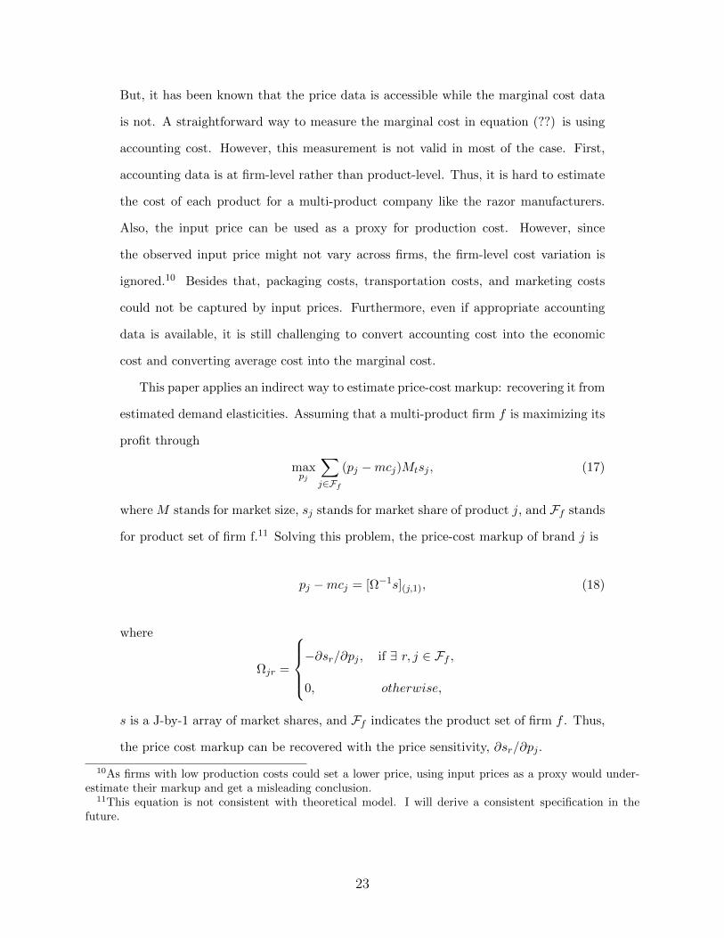
This paper applies an indirect way to estimate price-cost markup: recovering it from

estimated demand elasticities. Assuming that a multi-product firm f is maximizing its

profit through

maxpj

∑j∈Ff

(pj −mcj)Mtsj , (17)

where M stands for market size, sj stands for market share of product j, and Ff stands

for product set of firm f.11 Solving this problem, the price-cost markup of brand j is

pj −mcj = [Ω−1s](j,1), (18)

where

Ωjr =

−∂sr/∂pj , if ∃ r, j ∈ Ff ,

0, otherwise,

s is a J-by-1 array of market shares, and Ff indicates the product set of firm f . Thus,

the price cost markup can be recovered with the price sensitivity, ∂sr/∂pj .

10As firms with low production costs could set a lower price, using input prices as a proxy would under-estimate their markup and get a misleading conclusion.

11This equation is not consistent with theoretical model. I will derive a consistent specification in thefuture.

23

5.3 OLS Logit

5.3.1 Discrete Choice Model

Generally, ∂sr/∂pj can be estimated by regressing sr on pj . However, since demands

for all products are interactive, the market share of each product depends on not only

its own price but also the prices of all other brands. Thus, the curse of dimensionality

arises: if there are J products in a market, J2 price coefficients need to be estimated,

which is often too much.

The dimensionality problem calls for an alternative estimation strategy. This paper

is estimating the demand sensitivity with the discrete choice demand model which is

introduced by McFadden (1978). This model assumes that a consumer has the indirect

utility function:

uijt = α(yi − pjt) +Xjβ + ξjt + εijt, for j = 1, 2, ..., J, (19)

where yi stands for income of individual i, pjt stands for price of product j in market t,

Xj stands for observed characteristics of product j, ξjt stands for unobserved valuation

of product j which is common to all consumers in market t, and εijt is a mean-zero

stochastic term. For simplicity, equation (9) can be transformed into

uijt = αyi − δjt + εijt, (20)

, where δjt = pjt +Xjβ + ξjt.

Income effect is introduced in a linear form, αyi. Thus, different income level would

not make any difference to choice and the income term will be canceled out in following

steps.12 Also, the terms which do not vary by individuals, that is −αpjt + Xjβ + ξjt,

are denoted as δjt. Then δjt captures the mean utility of product j which is common

12If income effect is important, it can be modelled by a indirect utility which is concave to income, suchas BLP (1995) in which

uijt = ln(α(yi − pjt)) +Xjβ + ξjt + εijt.

24

to all consumers. The last term, εijt, captures individual deviation from mean utility.

An outside product is introduced to complete consumers’ choice set. The indirect

utility function of the outside option is:

ui0t = αyi − αp0t +X0tβ + ξ0t + εi0t

= αyi + εi0t.

(21)

Note that, the mean utility of outside option is normalized to be zero.

Product j would be selected if and only if

uijt > uirt, for r = 0, 1, ..., J, and r 6= j. (22)

In the real world, consumers’ choices are diverse; no brand can acquire the whole

market. Since all consumers sort the mean utilities in the same order, the diversity

can only be accounted by εijt.13 The implication of this assumption will be discussed

later.

When εijt follows Type I Extreme Value Distribution, the probability that an indi-

vidual i chooses product j is

sijt =exp (Xjtβ − αpjt + ξjt)∑Jr=0 exp (Xrtβ − αprt + ξrt)

. (23)

The coefficients can be estimated by matching predicted choice probability to ob-

served consumer purchase history.14

Generally, however, individual purchase history data is not readily accessible. An

alternative method is using predicted market share, instead of predicted choice proba-

13In this context, if the mean utility of product r is not the highest, then it is purchased by individual i∗

only when εi∗jt is high enough.14That is, using MLE to estimate the coefficients which have the highest probability to make observed

purchase history happened.

25

bility, to match the data.15 As equation (14) shows,

sjt =1

ns

ns∑i=1

exp (Xjtβ − αpjt + ξjt)∑Jr=0 exp (Xrtβ − αprt + ξrt)

=exp (Xjtβ − αpjt + ξjt)∑Jr=0 exp (Xrtβ − αprt + ξrt)

,

(24)

the predicted market share is assumed to be equal to the average choice probability of

individuals, which is numerically equal to choice probability.

Given the predicted and observed market shares, the coefficients can be estimated

by solving

minα,β||S − s(X, p, ξ;α, β)||. (25)

The objective function in equation (??) is non-linear to the coefficients. Solving non-

linear minimization problem by search procedure is costly. Also, the method of in-

strumental variables, in its most commonly used 2SLS form, cannot be applied to a

non-linear model. Therefore, the objective function of estimation problem should be

linearized. When the market share takes the form of equation (??), it is convenient to

apply log-linearization: taking log on both sides of equation (??) yields

ln(sjt) = −αpjt +Xjtβ + ξjt − ln(J∑r=0

eXrtβ−αprt+ξrt)

ln(s0t) = −ln(

J∑r=0

eXrtβ−αprt+ξrt)

(26)

Then taking difference between ln(sjt) and ln(s0t) yields

ln(sjt)− ln(s0t) = δjt ≡ Xjtβ − αpjt + ξjt (27)

15Some dataset, such as Nielsen Household Scanner Dataset, provide data about each shopping trip ofsample household. For the products which consumers do not purchase frequently, however, the shopping tripdata cannot be used directly. Consumers buy razors by several months. So in many of the trip observations,consumers did not purchase any of the razors. This does not mean they do not prefer any of the insidechoices. But discrete choice model treats it as that this consumer prefers outside option. So using individualshopping trip data may significantly underestimate mean utility of inside products.

26

Since Sjt and S0t are observed, equation (17) can be consistently estimated with the

ordinary least square regression when the structural residual term, ξjt, is stochastic

and uncorrelated with regressors.

5.3.2 Endogeneity

It is common that the price variable is correlated with the structural error term, ξjt;

that is, the price variable is endogenous. The endogeneity is usually from two sources:

unobserved product characteristics and simultaneity.

Some of the product characteristics are observable to the consumers but unobserv-

able to the researchers. When the unobserved product characteristics are correlated

with price, the price variable can be endogenous. For example, in the razor market,

the sharpness of the blade cannot be observed by the researchers. But the consumers

can perceive the sharpness when they use it. And they would like to pay more for a

sharper razors. Also, since it is costly to product the sharper blades, the sharpness is

correlated with the price. As a result, the price coefficient would be overestimated if

the unobserved quality is ignored.

As Nevo (2000, 2001) suggested, a brand fixed effect can be used to control for

the unobserved product characteristics. The brand fixed effect captures the product

characteristics that do not vary by market. Then the structural error term can be

decomposed as

ξjt = ξj + ∆ξjt (28)

where ξj stands for the brand fixed effect of brand j, and ∆ξjt is the market specific

deviation from the mean utility. Since the brand fixed effect captures all product

characteristics information, Xjt can be dropped out.Then equation (??) is transformed

into

ln(sjt)− ln(s0t) = −αpjt + ξj + ∆ξjt. (29)

Another source of the price endogeneity is the simultaneity problem; that is, the

27

price is endogenously determined by firms’ pricing conduct. Since the razor market is

highly concentrated, a firm is a price maker. In other words, the firm is able to react

to the consumers’ taste, ∆ξjt. Then a pricing function should be

pjt = cjt + f(∆ξjt), (30)

where cjt stands for the marginal cost, and f(·) is a markup function. In this case, the

OLS estimation of equation (??) is biased.

This paper applies the Hausman instruments, the average prices in adjacent areas,

to solve this problem. Due to common cost shifter, prices in adjacent areas are corre-

lated. Also, if ∆ξjt is independent across areas, pj,−t would be uncorrelated with ∆ξjt.

Thus, the prices of the brand in other areas are valid IVs.

5.3.3 Demand Elasticities

With Hausman instrumental variables, equation (??) can be consistently estimated

by a two-stage least squares regression. Furthermore, the estimated price coefficient

and the predicted market share can be used to calculate the price sensitivities,

∂sjt∂prt

=

−αsjt(1− sjt) if j = r,

αsjtsrt if j 6= r,

(31)

and the demand elasticities,

ηjrt =∂sjt∂prt

· prtsjt

−αpjt(1− sjt) if j = r,

αprtsrt if j 6= r.

(32)

Then, the price-cost markup can be derived by substituting the price sensitivity into

equation (??).

28

5.4 Random Coefficient Logit

5.4.1 Independence of Irrelevant Alternatives

In conditional logit model, the random disturbance term, εijt, is assumed to be

independent by observations, which means that a consumer’s taste on one brand has

nothing to do with his taste on another brand. This assumption, named as Indepen-

dence of Irrelevant Alternatives (IIA), implies several unrealistic conclusions.

As equation (??) shows, the cross elasticities depend only on market share and

price of product j. As it shows in Table (22), if Gillette reduces Fusion cartridge

price, all other products, such as Private Label disposable razors and Schick Hydro 5

cartridge which is Fusion’s close substitute, lose the same size of market share. On

the other hand, the own elasticity is close to −αpjt when the market share of each

brand is small. It implies that the demand for low price brand is inelastic, and then

the price-cost markup of low-price brand is high. Those implications are opposite to

common sense.

5.4.2 Individual-Specific Coefficients

One way to relax IIA assumption is to use the nested logit model. This model

assumes that, for example, a consumer makes a choice between the disposable razor

and non-disposable razor at first, then choose among three-blade, four-blade, or five-

bladed, and at last choose among brands. A problem with the nested logit model is that

the estimated substitution pattern heavily depends on the nesting which is determined

a priori.

A more complicated way is to let the coefficients of price and other product char-

acteristics vary across individuals. That is,

αi

βi

=

α

β

+ ΠDi, (33)

29

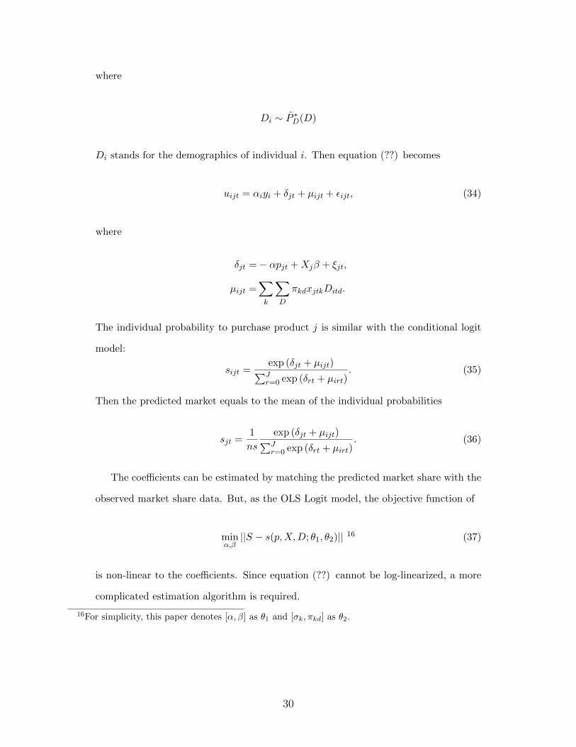
where

Di ∼ P ∗D(D)

Di stands for the demographics of individual i. Then equation (??) becomes

uijt = αiyi + δjt + µijt + εijt, (34)

where

δjt =− αpjt +Xjβ + ξjt,

µijt =∑k

∑D

πkdxjtkDitd.

The individual probability to purchase product j is similar with the conditional logit

model:

sijt =exp (δjt + µijt)∑Jr=0 exp (δrt + µirt)

. (35)

Then the predicted market equals to the mean of the individual probabilities

sjt =1

ns

exp (δjt + µijt)∑Jr=0 exp (δrt + µirt)

. (36)

The coefficients can be estimated by matching the predicted market share with the

observed market share data. But, as the OLS Logit model, the objective function of

minα,β||S − s(p,X,D; θ1, θ2)|| 16 (37)

is non-linear to the coefficients. Since equation (??) cannot be log-linearized, a more

complicated estimation algorithm is required.

16For simplicity, this paper denotes [α, β] as θ1 and [σk, πkd] as θ2.

30

5.4.3 Estimation Algorithm

The contraction mapping approach, introduced by Berry (1994), can be applied to

solve the estimation problem. This approach suggests that an approximation of mean

utility, δH·t , can be solved by computing the series

δh+1·t = δh·t + lnS·t − ln (s(δh·t; θ2)), h = 0, 1, ...,H, (38)

where H is the smallest integer such that ||δH·t − δH−1·t || is smaller than some tolerance

level. The approximation of mean utility, δH·t , is a function of the observed market

share,S·t, and unknown coefficients, θ2. Then the mean utility function is

δjt(S·t; θ2) = −αpjt +Xjβ + ξjt (39)

Unlike the conditional logit model, a generalized method of moments is applied to

estimate θ. The GMM error term is defined as

wjt = ∆ξjt ≡ δjt(S·t; θ2)− (−αpjt + xjtβ), (40)

Then the moment condition is

E[Z ′w(θ)] = 0, (41)

where Z consist of the exogenous regressors and Hausman instrumental variable. Then

the GMM estimate is

θ = argminθ

w(θ)′ZΦ−1Z ′w(θ), (42)

where Φ is a consistent estimate of E[Z ′ww′Z].

Equation (??) can be solved by a non-linear search over θ. To make the search

procedure more efficient, θ1 can be expressed as a function of θ2,

θ1 = (X ′LZΦ−1Z ′XL)−1X ′LZΦ−1Z ′δ(θ2). (43)

31

Then equation (32) can be solved by searching over θ2 only.

The estimation takes the following steps:

• Select starting points for δ and θ2. The starting point of δ can be set as the

predicted value of equation (??). The starting point of θ2 can be an arbitrary

value.

• Perform the contraction mapping in equation (??) with the observed market

share S·t and the starting points of δ and θ2. Keeping θ2 fixed at its starting

point, iterate the value of δ until || lnS − ln (s(δ; θ2))|| is small enough. Then we

get an updated δ as a function of θ2.

• Calculate the GMM error term in equation (??) with the starting point of θ2 we

got from step 1 and the value of δ we got from step 2. Then we have ω as a

function of θ2.

• Estimate the weighting matrix Φ = Z ′ωω′Z with ω we got from step 3.

• Using search algorithm to find a new value for θ2 in equation (??) with the error

term we got from step 3 and the weighting matrix we got from step 4. Then we

have a new value of θ2 and a value of GMM objective function according to this

θ2

• Return to step 2 and update θ2 with the value we got from step 5. Then repeat

step 2 to step 5, until the value of GMM objective function in step 5 is close

enough to zero.

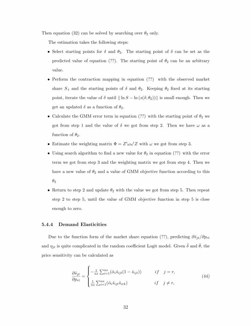
5.4.4 Demand Elasticities

Due to the function form of the market share equation (??), predicting ∂sjt/∂prt

and ηjt is quite complicated in the random coefficient Logit model. Given δ and θ, the

price sensitivity can be calculated as

∂sjt∂prt

=

− 1ns

∑nsi=1(αisijt(1− sijt)) if j = r,

1ns

∑nsi=1(αisijtsirk) if j 6= r,

(44)

32

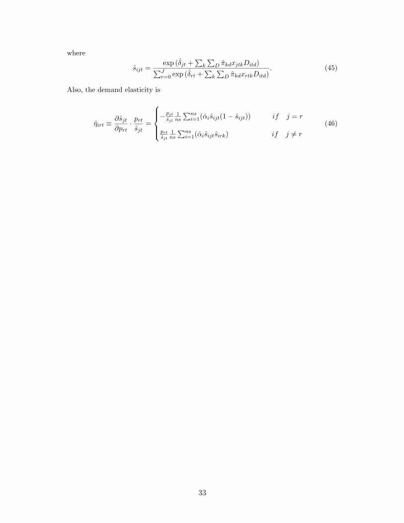
where

sijt =exp (δjt +

∑k

∑D πkdxjtkDitd)∑J

r=0 exp (δrt +∑

k

∑D πkdxrtkDitd)

. (45)

Also, the demand elasticity is

ηirt ≡∂sjt∂prt

· prtsjt

=

−pjtsjt

1ns

∑nsi=1(αisijt(1− sijt)) if j = r

prtsjt

1ns

∑nsi=1(αisijtsirk) if j 6= r

(46)

33

6 Results

6.1 Conditional Logit Results

As noted in section IV, the logit results cannot yield reliable price-cost markups.

However, due to computational simplicity, it is a useful method in evaluating the

instrumental variables and comparing the different specifications.

Table 5: Results from the Conditional Logit Model

(1) (2) (3) (4) (5) (6)

Price -0.494 -0.527 -0.572 -0.822 -0.922 -1.448

(0.018) (0.018) (0.021) (0.018) (0.018) (0.031)

Package Size 0.457 0.460 0.450 -0.052 -0.060 -0.175

(0.01) (0.009) (0.009) (0.007) (0.007) (0.009)

Handle Price 0.096 -0.093 -0.096 -0.026 -0.022 -0.017

(0.008) (0.008) (0.008) (0.005) (0.005) (0.005)

Cartridge 0.276 0.153 0.318 1.704 1.680 1.907

(0.063) (0.027) (0.064) (0.040) (0.038) (0.041)

Blades = 4 0.117 0.153 0.178 — — —

(0.027) (0.027) (0.028) — — —

Blades = 5 1.608 1.670 1.737 — — —

(0.035) (0.034) (0.038) — — —

Schick -1.488 -1.522 -1.560 — — —

(0.025) (0.025) (0.026) — — —

BiC -0.724 -0.765 -0.813 — — —

(0.030) (0.030) (0.032) — — —

Dummies:

Brand

Time

Instruments

1st stage R2 — — 0.97 — — 0.97

1st stage F-test — — 2920.53 — — 489.11

Observations 11088 11088 11088 11088 11088 11088

R2 0.60 0.61 0.61 0.86 0.87 0.99

34

Table (??) displays the results of the conditional logit model. Column (1) to (3)

are according to specification (??), in which the independent variables consist of the

observed product characteristics. The unobserved product characteristics are embed-

ded in the structural error term. Column (2) introduces a time fixed effect to control

for the trend and quarterly change of preference. Column (3) use the Hausman instru-

mental variables in a two-stage least squares regression. From column (1) to (3), the

price coefficient increases from −0.494 to −0.572 as expected, which implies that the

Hausman instruments alleviate the endogeneity caused by simultaneity problem.

Columns (4) to (6) are according to specification (??), in which a brand fixed

effect is introduced to control for the unobserved product characteristics and all no

market-invariant product characteristics are dropped. Comparing the price coefficients

in column (1) to (3) with those in column (4) to (6), we find the effect of including

brand dummies is significant, which implies that the brand fixed effect works well on

controlling for the endogeneity caused by unobserved characteristics.

In column (6), all the coefficients have desirable signs. Thus, it is an appropriate

benchmark to develop the BLP model.

6.2 BLP Results

6.2.1 Estimation

The specification of the BLP model is based on equation (??) which includes a

brand fixed effect to control for the unobserved characteristics and interactions between

product characteristics and individual demographics to allow for individual specific

coefficients. The individual demographics are sampled from the March CPS. The price

variable is instrumented by Hausman IV to control for the simultaneity problem.17

The coefficient estimates are computed by the procedure discussed in Section (??).

Table (??) shows the estimates of the preference parameters of the BLP model.

The preference means, denoted as α and β in equation (??), are presented in column

17The product characteristics variables and individual demographics variables have been discussed insection 5.3. The instrumental variables have been discussed in section 5.4.

35

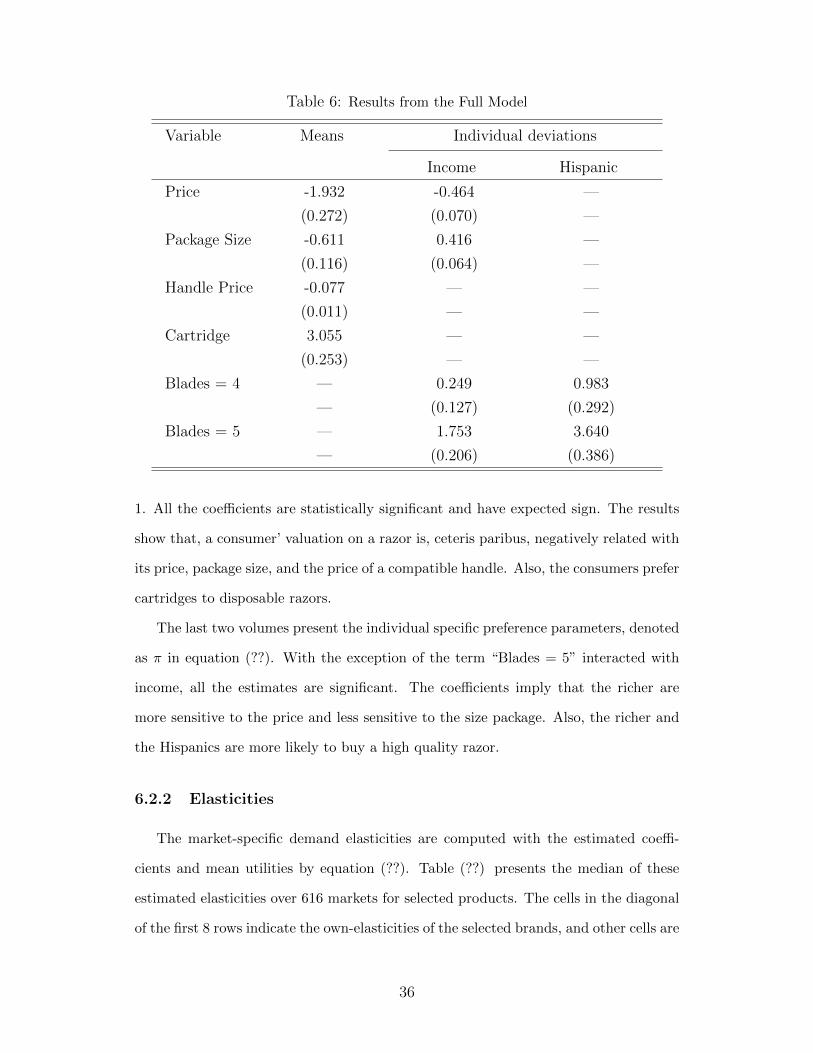
Table 6: Results from the Full Model

Variable Means Individual deviations

Income Hispanic

Price -1.932 -0.464 —

(0.272) (0.070) —

Package Size -0.611 0.416 —

(0.116) (0.064) —

Handle Price -0.077 — —

(0.011) — —

Cartridge 3.055 — —

(0.253) — —

Blades = 4 — 0.249 0.983

— (0.127) (0.292)

Blades = 5 — 1.753 3.640

— (0.206) (0.386)

1. All the coefficients are statistically significant and have expected sign. The results

show that, a consumer’ valuation on a razor is, ceteris paribus, negatively related with

its price, package size, and the price of a compatible handle. Also, the consumers prefer

cartridges to disposable razors.

The last two volumes present the individual specific preference parameters, denoted

as π in equation (??). With the exception of the term “Blades = 5” interacted with

income, all the estimates are significant. The coefficients imply that the richer are

more sensitive to the price and less sensitive to the size package. Also, the richer and

the Hispanics are more likely to buy a high quality razor.

6.2.2 Elasticities

The market-specific demand elasticities are computed with the estimated coeffi-

cients and mean utilities by equation (??). Table (??) presents the median of these

estimated elasticities over 616 markets for selected products. The cells in the diagonal

of the first 8 rows indicate the own-elasticities of the selected brands, and other cells are

36

cross-elasticities. Cell (m,n) indicates the elasticity of brand in row m with respect to

a price change of brand in column n. All the own- and cross-elasticities have desirable

signs and magnitudes.

37

Tab

le7:

Med

ian

Ow

nan

dC

ross

-Ela

stic

itie

s

Mac

h3

(D)

Mac

h3

Fusi

on(D

)F

usi

onQ

uat

tro

(D)

Quat

tro

Hydro

5(D

)H

ydro

5

Gille

tte

Mac

h3

(D)

-4.0

286

0.19

610.

0133

0.26

000.

0036

0.01

390.

0163

0.05

70

Gille

tte

Mac

h3

0.06

84-7

.054

30.

0129

0.90

990.

0060

0.03

740.

0411

0.18

82

Gille

tte

Fusi

on(D

)0.

0164

0.11

52-4

.871

30.

6743

0.00

270.

0118

0.04

450.

1530

Gille

tte

Fusi

on0.

0586

0.64

250.

0494

-11.

3863

0.00

670.

0373

0.10

870.

4726

Sch

ick

Quat

tro

(D)

0.06

010.

2617

0.02

660.

4580

-4.5

368

0.01

770.

0283

0.10

34

Sch

ick

Quat

tro

0.06

650.

5157

0.02

200.

7734

0.00

60-6

.652

00.

0439

0.17

55

Sch

ick

Hydro

5(D

)0.

0532

0.39

330.

0540

1.50

630.

0061

0.02

88-7

.271

00.

3586

Sch

ick

Hydro

50.

0554

0.57

310.

0497

1.87

380.

0065

0.03

460.

1027

-9.7

759

Gille

tte

Cust

omP

lus

3(D

)0.

0680

0.40

730.

0167

0.51

060.

0054

0.02

400.

0277

0.10

64

Gille

tte

Sen

sor

3(D

)0.

0666

0.43

990.

0159

0.54

490.

0054

0.02

540.

0287

0.11

43

Gille

tte

Mac

h3

Turb

o0.

0721

0.65

310.

0146

0.78

260.

0061

0.03

390.

0385

0.16

02

Gille

tte

Fusi

onP

roG

lide

0.05

770.

5780

0.05

191.

9596

0.00

680.

0352

0.10

820.

4461

Sch

ick

Xtr

eme

3(D

)0.

0611

0.59

000.

0123

0.69

320.

0050

0.02

950.

0328

0.14

18

Sch

ick

Hydro

30.

0688

0.48

700.

0155

0.60

140.

0056

0.02

730.

0309

0.12

39

BiC

Com

fort

3(D

)0.

0583

0.47

540.

0135

0.54

290.

0049

0.02

560.

0277

0.12

13

BiC

Com

fort

3A

dva

nce

(D)

0.06

540.

4042

0.01

530.

4873

0.00

520.

0239

0.02

680.

1066

BiC

Fle

x3

(D)

0.06

370.

5042

0.01

420.

6012

0.00

530.

0273

0.03

020.

1294

BiC

Fle

x4

(D)

0.06

360.

2804

0.02

830.

4899

0.00

530.

0194

0.03

040.

1106

38

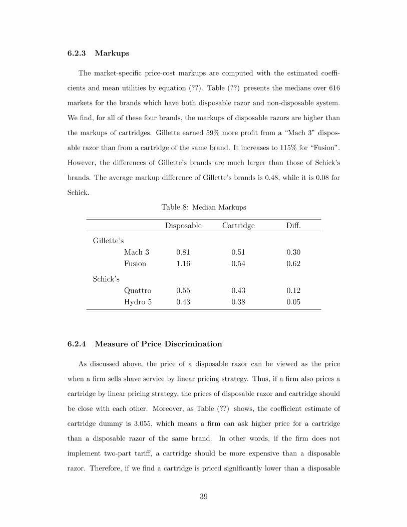
6.2.3 Markups

The market-specific price-cost markups are computed with the estimated coeffi-

cients and mean utilities by equation (??). Table (??) presents the medians over 616

markets for the brands which have both disposable razor and non-disposable system.

We find, for all of these four brands, the markups of disposable razors are higher than

the markups of cartridges. Gillette earned 59% more profit from a “Mach 3” dispos-

able razor than from a cartridge of the same brand. It increases to 115% for “Fusion”.

However, the differences of Gillette’s brands are much larger than those of Schick’s

brands. The average markup difference of Gillette’s brands is 0.48, while it is 0.08 for

Schick.

Table 8: Median Markups

Disposable Cartridge Diff.

Gillette’s

Mach 3 0.81 0.51 0.30

Fusion 1.16 0.54 0.62

Schick’s

Quattro 0.55 0.43 0.12

Hydro 5 0.43 0.38 0.05

6.2.4 Measure of Price Discrimination

As discussed above, the price of a disposable razor can be viewed as the price

when a firm sells shave service by linear pricing strategy. Thus, if a firm also prices a

cartridge by linear pricing strategy, the prices of disposable razor and cartridge should

be close with each other. Moreover, as Table (??) shows, the coefficient estimate of

cartridge dummy is 3.055, which means a firm can ask higher price for a cartridge

than a disposable razor of the same brand. In other words, if the firm does not

implement two-part tariff, a cartridge should be more expensive than a disposable

razor. Therefore, if we find a cartridge is priced significantly lower than a disposable

39

razor of the same brand, the firm intentionally lowers down its cartridge price on the

purpose of implementing two-part tariff.

Since the marginal costs of a disposable razor and a cartridge might be different,

it is necessary to partial out the cost difference from the price difference. Using the

markups in Table (??) and the average prices in Table (), I form a measure of two-part

tariff which is calculated as

Ratio =Markupdisposable −Markupcartridge

Pricedisposable − Pricecartridge(47)

This ratio evaluates the extent to which price difference is drove by markup difference.

The result shows, on average, over 90% of price difference of Gillette’s brands can be

explained by markup difference.

This conclusion can be strengthened by comparing the ratio of Gillette’s brands

and Schick’s brands. As discussed, a firm can implement two-part tariff only if it has

market power. Since the razor market is dominated by Gillette, other firms should not

use two-part tariff strategy. Thus, for any brand made by the rest firms in this market,

the ratio calculated with equation (??) should be small. Then I calculate the ratios of

two brands which sell both disposable razors and cartridges. I find the average ratio

of them is 25%, which is much smaller than Gillette’s.

To sum up, the empirical evidence is consistent with the explanation that Gillette

is implementing two-part tariff pricing strategy in men’s shaving razor market.

40

7 Conclusion

This paper uses a random-coefficient logit model to estimate the demand system of

men’s razors with market level sales data in the United States between 2015 to 2016.

The estimates are used to calculate the price-cost markups of each products. The result

shows that: First, the markup of cartridges are lower than the disposable razors of the

same brands. Second, the markup difference can contribute a large fraction of price

difference of Gillette’s brands. Last, the ratio of markup difference to price difference

of Gillette’s brands is much higher than that of Schick’s brands. This evidence is

consistent with the prediction of two-part tariff theory. In other words, it comes to a

conclusion that Gillette is using two-part tariff strategy in this market.

This conclusion can be generalized as that a tie-in sale can be used to implementing

two-part tariff, or inversely, the two-part tariff can take the form of tie-in sale.

41

References

Berry, Steven T. “Estimating discrete-choice models of product differentiation.” The

RAND Journal of Economics (1994): 242-262.

Berry, Steven, James Levinsohn, and Ariel Pakes. “Automobile prices in market equi-

librium.” Econometrica: Journal of the Econometric Society (1995): 841-890.

Bonnet, Celine, and Pierre Dubois. “Inference on vertical contracts between manufac-

turers and retailers allowing for nonlinear pricing and resale price maintenance.” The

RAND Journal of Economics 41, no. 1 (2010): 139-164.

Bonnet, Celine, and Pierre Dubois. “Identifying two part tariff contracts with buyer

power: empirical estimation on food retailing.” (2015).

Bowman Jr, Ward S. “Tying arrangements and the leverage problem.” Yale Lj 67

(1957): 19.

Burstein, M. L. “The Economics of Tie-In Sales.” The Review of Economics and Statis-

tics 42, no. 1 (1960): 68-73.

Chintagunta, Pradeep K., Marco Qin, and Maria Ana Vitorino. “Licensing and price

competition in tied-goods markets: An application to the single-serve coffee system

industry.” (2018).

Cohen, Andrew. “Package size and price discrimination in the paper towel market.”

International Journal of Industrial Organization 26, no. 2 (2008): 502-516.

Dube, Jean-Pierre, Jeremy T. Fox, and Che-Lin Su. “Improving the numerical per-

42

formance of static and dynamic aggregate discrete choice random coefficients demand

estimation.” Econometrica 80, no. 5 (2012): 2231-2267.

Gil, Ricard, and Wesley R. Hartmann. “Empirical analysis of metering price discrimi-

nation: Evidence from concession sales at movie theaters.” Marketing Science 28, no.

6 (2009): 1046-1062.

Hartmann, Wesley R., and Harikesh S. Nair. “Retail competition and the dynamics of

demand for tied goods.” Marketing Science 29, no. 2 (2010): 366-386.

Hausman, Jerry A. “Valuation of new goods under perfect and imperfect competition.”

In The economics of new goods, pp. 207-248. University of Chicago Press, 1996.

Lakdawalla, Darius, and Neeraj Sood. “Health insurance as a two-part pricing con-

tract.” Journal of public economics 102 (2013): 1-12.

Nevo, Aviv. “Measuring market power in the ready-to-eat cereal industry.” Economet-

rica 69, no. 2 (2001): 307-342.

Nevo, Aviv. “A practitioner’s guide to estimation of random-coefficients logit models

of demand.” Journal of economics & management strategy 9, no. 4 (2000): 513-548.

Oi, Walter Y. “A Disneyland dilemma: Two-part tariffs for a Mickey Mouse monopoly.”

The Quarterly Journal of Economics 85, no. 1 (1971): 77-96.

Picker, Randal C. “The razors-and-blades myth (s).” U. Chi. L. Rev. 78 (2011): 225.

Schmalense, Richard. “Monopolistic two-part pricing arrangements.” The Bell Journal

of Economics (1981): 445-466.

43

Schmalensee, Richard. “Pricing the razor: A note on two-part tariffs.” International

journal of industrial organization 42 (2015): 19-22.

Shepard, Andrea. ”Price discrimination and retail configuration.” Journal of Political

Economy 99, no. 1 (1991): 30-53.

Scott, Frank A., and Stephen O. Morrell. “Two-part pricing for a multi-product mo-

nopolist.” Economic Inquiry 23, no. 2 (1985): 295-307.

Verboven, Frank. “International price discrimination in the European car market.”

The RAND Journal of Economics (1996): 240-268.

Verboven, Frank. “Quality-based price discrimination and tax incidence: evidence

from gasoline and diesel cars.” RAND Journal of Economics (2002): 275-297.

Yin, Xiangkang. “Two-part tariff competition in duopoly.” International Journal of

Industrial Organization 22, no. 6 (2004): 799-820.

44