PREDICTING FUTURE RANGE EXPANSION OF WHOOPING CRANE (GRUS

AMERICANA) WINTER HABITAT USING LONG-TERM CENSUS AND

REMOTELY SENSED DATA

by

Nicole Aileen Davis, M.S.

A dissertation submitted to the Graduate Council of Texas State University in partial fulfillment

of the requirements for the degree of Doctor of Philosophy

with a Major in Aquatic Resources and Integrative Biology May 2019

Committee Members:

Thomas B. Hardy, Chair

M. Clay Green

Jennifer Jensen

Susan Schwinning

Elizabeth H. Smith

COPYRIGHT

by

Nicole Aileen Davis

2019

FAIR USE AND AUTHOR’S PERMISSION STATEMENT

Fair Use

This work is protected by the Copyright Laws of the United States (Public Law 94-553, section 107). Consistent with fair use as defined in the Copyright Laws, brief quotations from this material are allowed with proper acknowledgement. Use of this material for financial gain without the author’s express written permission is not allowed.

Duplication Permission

As the copyright holder of this work I, Nicole Aileen Davis, authorize duplication of this work, in whole or in part, for educational or scholarly purposes only.

DEDICATION

I dedicate this primarily to my Husband. He continued to remain patient and supportive

of my goals that at times can seem endless. I also dedicate this achievement to my

Daughter. Through her eyes, I have been able to view the natural world in a completely

new way. Without them, I would not have been able to overcome the obstacles that arose

during this pursuit.

v

ACKNOWLEDGEMENTS

I am grateful to my major advisor, Thomas B. Hardy, for allowing me the

opportunity to pursue research questions and modelling methods for a landscape and bird

species that intrigue me. He provided guidance and feedback throughout my doctoral

education that has allowed me to further progress as an ecologist. I am most appreciative

of his ability to remain patient with life changes and speed bumps that occurred along the

way, while also providing firm demands that encouraged me to continue forward

momentum to achieve my goal. I am also appreciative of Elizabeth H. Smith for her

endless knowledge of coastal processes and whooping crane ecology. She played a large

role in connecting me with my major advisor and countless others in the whooping crane

world. Thanks to Thomas B. Hardy and Elizabeth H. Smith I was given the opportunity

to pursue my research goals while also working with a fascinating endangered species.

I would like to thank Jennifer L. Jensen for her knowledge of remote sensing and

spatial analyses. Her guidance provided me with new inspiration and the ability to obtain

new skills to improve my understanding of spatial ecology. I am also appreciative of M.

Clay Green for his knowledge of spatial ecology and his guidance through the doctoral

process. I would also like to thank Susan Schwinning for her knowledge and enthusiasm

of ecological modelling that inspired the grid-based models in Chapter IV.

I am grateful to the U.S. Fish and Wildlife Service for providing me with a long-

term whooping crane dataset, and to Andrew Sansom for supporting my dissertation

research involving whooping cranes. I am indebted to Tom V. Stehn for his incredible

vi

knowledge on the wintering ecology of the Aransas-Wood Buffalo whooping crane

population. He provided insightful ideas and engaged in thoughtful discussion that

greatly improved my dissertation. I am also grateful to many members of the

International Crane Foundation, specifically Rich Beilfuss, Kim Smith, and Dorn Moore.

Each one of them provided me with inspiration, knowledge, and great conversations that

kept me appreciative of my research and on track to succeed.

Again, I am most grateful for my husband and his encouragement throughout my

pursuit of higher education. He reminds me of my strengths when I need it the most and

keeps me standing when my strength is no longer enough.

This research was financially supported by the Coypu Foundation, Texas State

University Department of Biology, and the Texas State University Graduate College.

vii

TABLE OF CONTENTS

Page

ACKNOWLEDGEMENTS .................................................................................................v

LIST OF TABLES ............................................................................................................. ix

LIST OF FIGURES ........................................................................................................... xi

LIST OF ABBREVIATIONS .......................................................................................... xiv

ABSTRACT .................................................................................................................... xvii

CHAPTER

I. WHOOPING CRANE (Grus Americana) LIFE HISTORY, HABITAT, AND

STATUS GOALS ........................................................................................1

Biology .........................................................................................................1 Life History ..................................................................................................2 Wild Population ...........................................................................................4 Previous Population Studies ........................................................................6 Previous Space-Use Research ......................................................................9 Dissertation Objectives ..............................................................................12

II. EVALUATING WHOOPING CRANE WINTER TERRITORIES USING

HOME RANGE ESTIMATORS ...............................................................17

Whooping Crane Data ................................................................................22 Methods......................................................................................................23 Home Range and Core Areas ................................................................25 Conceptual Model Development ..........................................................28 Results ........................................................................................................29 Discussion ..................................................................................................30

viii

Management Implications .....................................................................36

III. WINTER WHOOPING CRANE DISTRIBUTION MODEL ALONG THE

TEXAS COAST.........................................................................................49

Methods......................................................................................................51 Whooping Crane Data ...........................................................................51 Determining Study Area Extent ............................................................53 Ecological and Environmental Data Layers .........................................54 Analyses ................................................................................................61 Results ........................................................................................................67 Discussion ..................................................................................................72 Management Implications .....................................................................80

IV. EVALUATINGTHE WINTER RANGE CARRYING CAPACITY IN

ARANSAS-WOOD BUFFALO WHOOPING CRANE POPULATION

USING MONTE CARLO SIMULATION ..............................................103

Territories and Carrying Capacity ...........................................................105 Methods....................................................................................................108

Suitability Thresholds and Area...................................................110 Territory Simulations ...................................................................111 Evaluation of Habitat Use and Conservation ...............................113

Results ......................................................................................................114 Discussion ................................................................................................116

APPENDIX SECTION ....................................................................................................133

LITERATURE CITED ....................................................................................................153

ix

LIST OF TABLES

Table Page

1. Dominant food items consumed by wintering whooping cranes in Texas ...................14

2. Aerial survey data from winter 1988-1989 used for the analyses ................................39

3. Identification of individually banded whooping cranes from

winter 1988-1989 used to develop home range and core area estimates ...........................40

4. Land cover types located within winter whooping crane home ranges ........................42

5. List of variables included in the analyses of winter whooping

crane home range and core area sizes ................................................................................44

6. Set of selected models developed to estimate key variables

influencing home range and core area sizes of wintering whooping cranes ......................45

7. Modified land cover classes compared to the original

Composite Habitat Type Dataset (CHTD) .........................................................................83

8. All environmental and ecological data layers used in the full model (Model 1) ..........84

9. Total area of mesohabitat classes used in the whooping crane distribution model ......87

10. Results from six winter whooping crane species distribution models developed to

predict the probability of whooping crane occurrence ......................................................88

11. Variable importance for the final species distribution model (Model 6) ....................89

12. Total number and average size of whooping crane core areas by

landform comprising the winter range for various winters between 1950 and 2006 .......120

x

13. Estimated average minimum territory sizes and total number of

potential territories per landform within the current winter range ...................................121

14. Cumulative frequency of winter suitability values occupied by paired/family

whooping cranes ..............................................................................................................122

15. Fixed and Monte Carlo core area sizes and the simulated

carrying capacity for each landform ................................................................................123

xi

LIST OF FIGURES

Figure Page

1. The historic and current range of the whooping crane (Grus americana) in North

America ..............................................................................................................................15

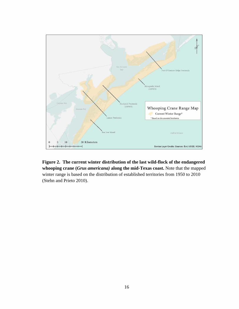
2. The current winter distribution of the last wild-flock of the endangered whooping

crane (Grus americana) along the mid-Texas coast ..........................................................16

3. Average home range and core area sizes of whooping cranes wintering along the

Texas Coast in 1988-1989 .................................................................................................46

4. Home ranges and distribution of subadult (top) and paired/family (bottom)

whooping cranes within the winter range along the Texas coast in 1988-1989 ................47

5. Core areas and distribution of paired/family whooping cranes within

the winter range along the Texas coast in 1988-1989........................................................48

6. Extent of the study area developed for this dissertation ...............................................91

7. Spatial extent of the modified mesohabitat data layer ..................................................92

8. Hydric soil data layer created from reclassifying U.S. Department of Agriculture’s

Natural Resource Conservation Service soil data and the

National Hydric Soils List for the state of Texas ...............................................................93

9. Example of the Texas Water Development Board’s nodes

located within the study area to develop TxBLEND salinity data .....................................94

10. Average salinities within the study area interpolated from Texas Water Development

Board’s TXBLEND data for winter months from 2003-2004 to 2009-2010 ....................95

xii

11. Results from the Principal Component Analysis (PCA) created in R statistical

software using ‘princomp’ and 33 of the 36 variables used in

the full Species Distribution Model (SDM) .......................................................................96

12. Modified mesohabitat classes within the San Antonio Bay and

Matagorda Bay systems .....................................................................................................97

13. Winter whooping crane suitability values within the study area

from four species distribution models comprised of different variables ...........................98

14. Marginal response curves for the four environmental variables that contributed

the most to wintering whooping crane distribution based on results from Model 5 ..........99

15. Results from jackknife test in Maxent for Model 6 ..................................................100

16. Winter whooping crane suitability values within the study area from

Model 6 and deep open water ..........................................................................................101

17. Predicted habitat suitability (low, medium, or high) from Model 6 results ..............102

18. Schematic of initial steps executed by both simulation models to

establish territories based on occupancy and suitability values .......................................124

19. Probability density function curves for winter suitability values occupied by

paired/family (top) and subadult (bottom) whooping cranes from 1950 to 2011 ............125

20. Winter suitability values preferred by family/paired and subadult whooping cranes

based on cumulative frequency of historic location data

and estimated suitability values within the study area .....................................................126

xiii

21. Comparison of established core areas using two different

expansion methods in the simulation models ..................................................................127

22. Simulated whooping crane core areas established within

the current winter range compared to mapped territories ................................................128

23. Simulated whooping crane core areas established within

the current winter range using the Monte Carlo modelling approach .............................129

24. Simulated whooping crane core areas established on

each landform within the current winter range ................................................................130

25. Example of simulated whooping crane core areas

on Blackjack and Lamar Peninsulas ................................................................................131

26. Suitable whooping crane habitat in relation to protected

areas located within the study area ..................................................................................132

xiv

LIST OF ABBREVIATIONS

Abbreviation Description

AIC Akaike Information Criterion

ANWR Aransas National Wildlife Refuge

AUC Area Under the Receiver-Operator Curve

AWBP Aransas-Wood Buffalo population

BHA Benthic Habitat Atlas

C5_high Category 5 Hurricane at High Tide

CHTD Composite Habitat Type Dataset

CONTIG Patch Contiguity

CVh Likelihood Cross Calidation

CWS Canadian Wildlife Service

ECON Edge Contrast

ED Edge Density

EMST Ecological Mapping System of Texas

ENMtools Ecological Niche Modeling Tools

ENVI Exelis Visual Information Solutions

DEM Digital Elevation Model

GCPLCC Gulf Coast Prairie Landscape Conservation

Cooperative

GIS Geospatial Information Systems

xv

GME Geospatial Modelling Environment

HSM Habitat Suitability Models

IDW Inverse Distance Weighting

Maxent Maximum Entropy Software

MCP Minimum Convex Polygon

MFI Mean Fractal Index

Mmhos/cm Millimho Per Centimeter

MOM Maximum of the Maximum Envelope of High

Water

MSIDI Modified Simpson’s Diversity Index

NAIP National Agriculture Imagery Program

NED National Elevation Dataset (USGS)

NLCD National Land Cover Dataset

NOAA National Oceanic and Atmospheric Association

NRCS Natural Resource Conservation Service

NTCHS National Technical Committee for Hydric Soils

NWI National Wetland Inventory

PA Patch Area

PAD-US Protected Areas Database (USGS)

PCA Principle Component Analysis

PROX Patch Proximity

xvi

PVA Population Viability Analyses

RSF Resource Selection Function

SDM Species Distribution Model

SLOSH Sea, Land, and Overland Surges from

Hurricanes model

SSURGO Soil Survey Geographic Database

TNRIS Texas Natural Resources Information System

TPWD Texas Parks and Wildlife Department

TWDB Texas Water Development Board

TxBLEND 2-dimensional Hydrodynamic Model for Texas

(TWDB)

TXDOT Texas Department of Transportation

USDA U.S. Department of Agriculture

USFWS U.S. Fish and Wildlife Service

USGS U.S. Geological Survey

WBNP Wood Buffalo National Park

WSS Web Soil Survey

wi Akaike Weights

xvii

ABSTRACT

The whooping crane (Grus americana) is one of the most threatened crane species

in the world and has been identified as an endangered species since 1967. The last wild-

population of the whooping crane, the Aransas-Wood Buffalo Population (AWBP),

breeds in Wood Buffalo National Park and surrounding areas in the Northwest Territories

of Canada and migrates 2,500 km through the Central Flyway to their wintering grounds

within the Aransas National Wildlife Refuge and surrounding areas on the Texas Coast.

The Endangered Species Act (ESA) recovery plan for this species outlines objectives to

down-list the species from endangered to threatened status, including an objective for a

self-sustaining wild population size of at least 1,000 individuals, including 250 breeding

pairs. However, the feasibility of meeting this objective requires an assessment of space-

use by wintering whooping cranes and of the amount of available habitat within the

winter range to support the recovery goal population size.

Historic location data for 42 color-banded whooping crane individuals were used

to analyze space-use strategies by three identified classes of cranes during the winter

season; i.e., subadult (immature), associated (non-mating pair), and paired/family (mating

pair). Space-use was analyzed by estimating winter whooping crane home range and

core area extents from kernel density estimators. The resulting home range estimates

supported previous descriptions based on observation data of the distribution of the three

identified classes on the wintering grounds. The resulting core area estimates yielded a

similar spatial distribution as winter territories identified by U.S. Fish and Wildlife

xviii

Service annual winter monitoring, and identified a positive relationship between core area

size and land cover diversity.

To further evaluate the suitability of habitat for winter whooping cranes, Maxent

software was used to create a winter whooping crane distribution model. The species

distribution model was developed from over 5,000 whooping crane locations from six

winter seasons and 35 environmental and ecological data layers that were considered to

be potentially significant factors relating to the ecology of wintering whooping cranes.

Environmental layers included salinity levels, hydric soils, and mesohabitats based on

land cover characteristics for the extent of the study area. Ecological data included GIS-

derived spatial layers such as distance from road and development, percent vegetative

cover, and landscape metrics (patch density, patch diversity, and edge density).

Correlation and principle component analyses, and a stepwise variable reduction method

were used to determine the most parsimonious model with the minimum number of

discriminatory variables.

The final winter whooping crane distribution model included 11 data layers that

matched observed whooping crane winter locations (AUC=0.824 ±0.005). Based on the

final model, winter whooping crane distribution is negatively influenced by distance from

seagrass, distance from estuarine vegetated marsh, patch contiguity, average density of

road, and distance to woody habitat, and probability of occurrence increased with

distance from anthropogenic development, percent estuarine vegetated marsh, and

distance from road. Furthermore, results from the model suggest more suitable whooping

xix

crane winter habitat is located northeast of their current range and that more than 181,000

ha of highly suitable habitat is located within our study area, which exceeds the 125,000

ha of habitat targeted for conservation by the U.S. Fish and Wildlife Service to have

enough winter habitat for 1,000 individual whooping cranes (USFWS 2012).

In the final chapter, a grid-based simulation model was developed to evaluate

carrying capacity for five distinct landforms that comprise the assumed current winter

whooping crane range. Fixed minimum average territory sizes and randomized territory

sizes following a Monte Carlo method were used to determine how many territories could

be established by paired/family whooping cranes based on the spatial mosaic of available

suitable habitat. Suitable habitat was further refined by fitting a probability density

function to whooping crane observations and computed suitability values based on long-

term winter whooping crane location data. Paired/family whooping cranes were

determined to occupy habitat with suitability values >0.426. This threshold suitability

value was selected based on the probability density function relationship. The grid-based

model includes three preliminary rules to create territories, including analysis of a raster

stack comprised of an occupancy layer, suitability values, and unique cell numbers. The

model allowed a pair to start at one randomly chosen raster cell from the raster stack that

was unoccupied and had a suitability value greater than the threshold. The model then

used a spatially coherent adjacent suitable cell search function to expand territories into

surrounding suitable cells. Once the territory size was met for the existing pair, the next

pair randomly selected a suitable starting cell to establish a territory, and this process

xx

continued until no more territories could be established on each of the five landforms.

Simulation using the Monte Carlo methods consistently estimated a greater

number of potential territories on each landform compared to the fixed-territory size

simulation. In total, the Monte Carlo method concluded a total of 159 territories could be

established within the current range of winter whooping cranes, which equates to 318

reproductive pairs. However, only 47% of the total amount of suitable habitat for

paired/family whooping cranes was included in the simulated territories. Lastly,

approximately 186.3 km2 of suitable habitat for paired/family whooping cranes is located

within protected areas, which leaves approximately 296.9 km2 of suitable habitat for

territorial whooping cranes that are not protected on the winter grounds. These

simulations are the first to use habitat suitability and space-use strategies in the prediction

of carrying capacity of whooping crane wintering grounds. With the addition of more

space-use strategies that will come from improved data collection methods, these

simulation models can be modified to further evaluate habitat use and carrying capacity

within the winter range of the endangered AWBP and assist in predicting future range

expansion as the population increases towards down-listing goals.

.

1

I. WHOOPING CRANE (Grus americana) LIFE HISTORY, HABITAT,

AND STATUS GOALS

Gruidae, the crane family, includes fifteen species of cranes distributed across the

world, with at least one crane species present on every continent except South America

and Antarctica (Meine and Archibald 1996). Two crane species are present within North

America, the sandhill crane (Grus canadensis) and the whooping crane (Grus

americana). Whooping cranes have remained listed as an endangered species since 1967

despite countless conservation efforts. This chapter explains the general biology and life

history of whooping cranes with an emphasis on their wintering grounds in the state of

Texas and discusses the importance of conservation efforts implemented on the wintering

grounds to reach Endangered Species Act Recovery Plan down-listing goals for this

species (Canadian Wildlife Service [CWS] and USFWS 2007).

Biology

Whooping cranes are the tallest birds in North America. They reach an average

height of 1.5 m tall, have a wingspan between 2.1 to 2.4 m, and weigh between 6.4 to 7.3

kg. Adult birds have white plumage and black wing tips identifiable when in flight and

can be field identified by the presence of a red patch on their forehead, a black mustache,

and black legs. Juvenile birds resemble adult whooping cranes in terms of their size but

can be distinguished from adults by the presence of brown or buff feathers (Allen 1952).

The life span of whooping cranes in the wild is approximately 22-24 years (Binkley and

Miller 1980). Exceptions include a female observed to reach 30 years old in the wild

(Gil-Weir et al. 2012) and the “Lobstick” male predicted to have reached 33 years of age

in the wild (Tom Stehn, U.S. Fish and Wildlife Service [USFWS], pers. comm.).

2

Whooping cranes have a low recruitment rate (USFWS Staff 1994). They reach

sexual maturity at two or three years of age but do not produce successful egg clutches

until the age of four (USFWS Staff 1994; Gil-Weir et al. 2012). They are primarily

monogamous but may form a new pair after the death of a mate. Each pair usually

produces one clutch of two eggs early in the breeding season, with only one chick

surviving, on average, due to aggressive sibling behavior (Miller 1973) and predation

(USFWS Staff 1994). Both parents incubate eggs for approximately 29 days before

hatching, and biparental care occurs which appears to be necessary for successful rearing

of young (USFWS Staff 1994). Whooping crane chicks are precocial; they grow to full

adult size and are ready for flight in approximately three months.

Life History

The whooping crane population was estimated to be close to 1,300-1,400

individuals in the 1860-70’s (Allen 1952), and potentially larger before European

settlement (CWS and USFWS 2007; BirdLife International 2012). By 1941, the last

remaining wild whooping crane population was comprised of only 15 individuals in one

distinct population, the smallest number of individuals documented for the species (CWS

and USFWS 2007). Whooping cranes were listed as ‘threatened with extinction’ by the

newly passed Endangered Species Preservation Act of 1967. Even though the wild

population has grown exponentially since 1941 (Gil-Weir et al. 2012; Butler et al. 2013),

whooping cranes remain listed as endangered under the Endangered Species Act of 1973

(USFWS 2012; BirdLife International 2012). Their continued status as an endangered

species is attributed to habitat loss and degradation, power lines, and illegal hunting

(CWS and USFWS 2007; Environment Canada 2007).

3

Based on fossil records and observational data, whooping cranes historically had a

broad distribution in the United States and Mexico (Allen 1952; Meine and Archibald

1996). Their historical southern winter range once encompassed the high grasslands of

Mexico and eastward into the brackish coastal marshes of Louisiana as well as along the

Atlantic Coast from Florida to the Carolinas (Allen 1952) (Figure 1). As the population

declined, so did their breeding and wintering ranges. The last wild-flock of whooping

cranes currently migrate 4,000 km through the Central Flyway from their breeding

grounds in northern Canada to their wintering grounds along the Texas Coast (Allen

1952). The natural breeding ground for whooping cranes is located in the north–central

region of Canada within Wood Buffalo National Park (WBNP) and the natural wintering

ground is located on Blackjack Peninsula within the Aransas National Wildlife Refuge

(ANWR) (Allen 1952; Archibald 1975). As the whooping crane population has

increased, their breeding and wintering grounds have extended into suitable habitat in

surrounding areas (CWS and USFWS 2007; Stehn and Prieto 2010).

Mature, adult whooping cranes exhibit site fidelity and establish territories in the

same relative locations within the breeding and wintering grounds (Allen 1952; Stehn and

Johnson 1987; Kuyt 1993). However, territory sizes and their habitat composition differ

considerably between the breeding and wintering seasons (Allen 1952; USFWS 1994).

Kuyt (1993) considers the territories established by whooping crane pairs on the breeding

grounds as home ranges that are approximately 12-19 km2 when isolated from other

individuals and 3-4 km2 when nesting areas are dense. These territories consist of

freshwater wetland complexes that are visually open and have a high density of ponds

(Timoney 1999). On the wintering grounds, territory size is more variable and are

4

associated primarily with salty- to brackish-wetland environments (Allen 1952; Stehn and

Johnson 1987; Bonds 2000). Moreover, whooping crane pairs display distinct territorial

behavior on the wintering grounds and defend their established territory from

neighboring pairs and other individuals (Allen 1950; Stehn and Johnson 1987).

Immature whooping cranes that have yet to form a pair bond are termed

subadults. Subadults are non-territorial and gregarious while on the wintering grounds,

forming cohorts on the perimeter of occupied territories. Once subadults have reached

sexual maturity and form a pair bond, they appear to develop a new territory close to the

parental territory of the male (Stehn and Johnson 1987; Stehn and Prieto 2010). Sharing

of territories has also been observed among pairs and family groups (Blankenship 1976),

although not as common a behavior as territorial defense.

Wild Population

Today, four whooping crane populations are geographically distinguishable in the

United States. This includes three experimental, reintroduced populations known as the

Eastern Migratory population, the Florida Non-Migratory population, and the Louisiana

Non-Migratory population, and one migratory population known as the Aransas-Wood

Buffalo population (AWBP), which is the last wild population of whooping crane. The

AWBP is a remnant of the last 15 whooping cranes found in the wild in the 1940s and is

the only self-sustaining population in the world. Based on surveys conducted by the

USFWS, the AWBP consists of approximately 505 individuals, as of the winter of 2017-

2018 (Butler and Harrell 2018). A total of approximately 849 whooping cranes are still

extant including birds in captivity and reintroduced populations such as the Eastern

5

Migratory Population, Louisiana Non-Migratory Population, and Florida Non-Migratory

Population (International Crane Foundation [ICF] 2018).

When the USFWS first started census surveys in 1950, all AWBP territories were

located on Blackjack Peninsula within the ANWR (referred to as the Blackjack Unit). As

the population increased, territory sizes on ANWR gradually decreased and new

territories became established within nearby areas by pioneer whooping crane pairs

(Stehn and Johnson 1987). By 1971, the winter range had expanded from the historical

territories on the Blackjack Unit to four adjacent landforms within the central Texas coast

(Stehn and Johnson 1987; Kuyt 1993). By 1990, 18 whooping crane territories were

recorded on the Blackjack Unit, one on Lamar Peninsula, five on San Jose Island, nine on

Matagorda Island within the ANWR (referred to as the Matagorda Unit), and four on Port

O’Connor Ridge Peninsula (referred to as Welder) (Stehn and Prieto 2010).

After comparing the number of whooping crane territories and their average sizes

over multiple winter seasons, Stehn and Prieto (2010) concluded that the Blackjack Unit

had reached total territory capacity by the winter of 1990. They documented only two

new territories on the Blackjack Unit between the winters of 1990 and 2007, and a

minimum average territory size of 1.0 km2. Using data from winter territories throughout

the winter range, Stehn and Prieto (2010) estimated the average AWBP territory size to

be 1.7 km2 and estimated a carrying capacity of 1,156 individuals for the area then

occupied by the population and adjacent, suitable salt marsh areas that birds could expand

into within a 111-km radius of the ANWR. The 111-km radius was estimated based on

the spatial extant of assumed suitable marsh areas that could support an additional 580

whooping cranes.

6

The current AWBP winter range includes the Blackjack Unit, Matagorda Unit, as

well as San Jose Island, Seadrift-Port O’Connor Ridge Peninsula (also referred to as

Welder), and Lamar Peninsula along the Texas Gulf Coast (Figure 2). Territories

primarily occur in salt marsh habitat adjacent to or within open water areas suitable for

foraging where the variability in territories reflect different methods of foraging

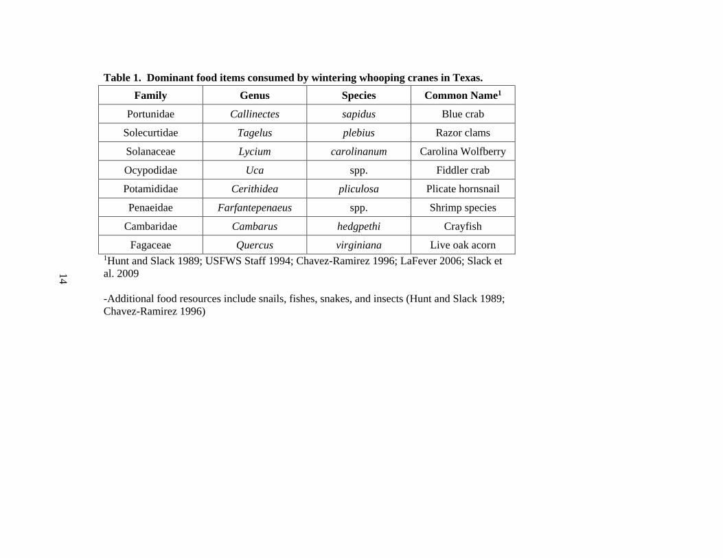
dependent on the type of prey or food item available (Allen 1952). Dominant food items

within the winter range are included in Table 1. Blue crabs are their primary food item

when tidal flats are flooded (Blankenship 1976), as well as Carolina wolfberry (Lycium

carolinianum) during fall and winter seasons (Hunt and Slack 1989; Chavez-Ramirez

1996; Wozniak et al. 2012), whereas multiple clam species are the predominant food item

when tides and associated water depths are low (Blankenship 1976; USFWS Staff 1994).

Availability of blue crabs and Carolina wolfberry have been correlated with fluxes in

freshwater inflows that affect the salinity of coastal marsh areas utilized by whooping

cranes in the winter (Hamlin 2005; Wozniak et al. 2012).

Previous Population Studies

Whooping cranes are listed as endangered because of concomitant biological and

anthropogenic factors such as human-induced land cover change from native grasslands

and prairie pothole wetlands into agriculture (Allen 1952) and hunting pressure (USFWS

Staff 1994). With only one last wild population present since 1950, whooping cranes are

one of the rarest crane species. Not surprisingly, they have drawn considerable attention

from the science community and have been intensively studied throughout their range

(Allen 1952; Bishop and Blankenship 1981; Howe 1987; Stehn and Johnson 1987;

Armbruster 1990; Stehn 1992; Kuyt 1993; USFWS Staff 1994; Chavez-Ramirez 1996;

7

Meine and Archibald 1996; Mirande et al. 1997; Timoney 1999; Bonds 2000; Austin and

Richert 2005; LaFever 2006; USFWS Staff 2007; Bishop et al. 2010, unpublished data;

Stehn and Prieto 2010; Gil-Weir et al. 2012; Wozniak et al. 2012; Butler et al. 2013;

Butler et al. 2017; Pearse et al. 2017).

Exponential growth of the last wild whooping crane population, the AWBP, is a

result of multiple conservation strategies including international habitat protection and

hunting restrictions (USFWS Staff 2012). Despite population growth, whooping cranes

remain an endangered species and no delisting criteria has been determined (USFWS

2012). A recovery plan with measurable down-listing criteria, from endangered to

threatened, is outlined in the International Recovery Plan for the Whooping Crane (Grus

americana) Third Revision (CWS and USFWS 2007). The primary objective is to

‘establish and maintain self-sustaining populations of whooping cranes in the wild that

are genetically stable and resilient to stochastic environmental events’. Measurable

criteria to determine if this objective is successful vary and depend on the size and

sustainability of the wild population as well as the success of reintroduced populations

(CWS and USFWS 2007; USFWS 2012). The remainder of this section as well as this

dissertation focuses on the AWBP and the ability of this population to meet the Recovery

Plan’s Alternative Criterion 1B: the AWBP being self-sustaining and remain above 1,000

individuals with at least 250 breeding pairs. The USFWS estimated the AWBP

comprises 505 whooping cranes based on survey results from the winter of 2017-2018

(Butler and Harrell 2018).

Several demographic studies and associated future population size projections

have been conducted for the whooping crane using data from the AWBP (Miller et al.

8

1974; Binkley and Miller 1980, Binkley and Miller 1983; Boyce 1987; Brook et al. 1999;

Staples et al. 2004; Gil-Weir et al. 2012; Butler et al. 2013). These studies have used

Monte Carlo simulations and population viability analyses (PVAs), which incorporate

fecundity rates, breeding success, and survival rates, to generate predictions. However,

different modeling approaches and assumptions have resulted in significantly different

projections (Brook et al. 1999; Gil-Weir 2006).

Mirande and others (1997) predicted the AWBP would reach 1,000 individuals by

the year 2035 if population growth were to continue at the same rate as previously

observed. By contrast, two more recent models predicted that the population would not

reach 1,000 individuals until after 2040 (Gil-Weir 2012; Butler et al. 2013). Gil-Weir

and others (2012) developed a population analysis to project whooping crane population

size using demographic data from 12 unique cohorts and with two different wintering

ground carrying capacity estimates. They concluded the population would not exceed the

down-listing goal of 1,000 individuals until the mid-2060s. Using Monte Carlo

simulations, Butler and others (2013) similarly determined that the probability of the

whooping crane population exceeding 1,000 individuals before 2040 was close to zero.

These estimates are essential for conservation managers to determine future habitat

conservation goals that will support the project population size of wintering whooping

cranes.

The amount of suitable breeding habitat does not limit the future survival and

distribution of whooping cranes (Tischendorf 2004). However, the amount of suitable

winter habitat is less definitive and was postulated as a limiting factor to population

growth (Binkley and Miller 1983). Using average territory sizes and estimated area of

9

salt marsh habitat within the winter range occupied by whooping cranes in the winter of

2006-2007, Stehn and Prieto (2010) estimated the winter range could support up to 576

individuals. Further, an additional 580 individuals could be supported by including non-

contiguous salt marsh habitat within a 111-km radius from the ANWR, resulting in an

overall carrying capacity of 1,156 individuals within a 111-km distance to the ANWR

(Stehn and Prieto 2010; USFWS Staff 2012).

Overall, the proposed goal of 1,000 whooping crane individuals would require an

additional 56,454 ha (139,500 acres) of salt marsh, of which only 12,950 ha (32,000

acres) is currently protected within the winter range on ANWR including areas protected

by additional conservation easements on adjacent private lands (USFWS Staff 2012).

However, assuming that additional suitable adjacent habitats to the ANWR are

accessible, and including effects from predicted sea level rise, sufficient winter habitat is

potentially available to support target population increases (Chavez-Ramirez and Wehtje

2012).

Previous Space-Use Research

Previous studies on the AWBP have focused on population viability or growth

(Binkley and Miller 1980, Binkley and Miller 1983, Binkley and Miller 1988; Brook et

al. 1999; Gil-Weir et al. 2012; Butler et al. 2013), food energetics (Hunt and Slack 1989;

Chavez-Ramirez 1996; Hamlin 2005; LaFever 2006), habitat suitability during migration

(Armbruster 1990; Austin and Richert 2005; Farmer et al. 2005), and on the breeding

grounds (Timoney 1999). Qualitative research, mostly by USFWS Biologists, has been

conducted within the AWBP’s winter range to evaluate habitat selection, spatial patterns

in whooping crane territory development, and carrying capacity, as well as predicting

10

future winter range expansion.

Territory sizes are highly variable throughout the winter range and predicted to be

larger in areas of poorer habitat quality, such as some areas characterized outside the

ANWR (Stehn and Prieto 2010). Wintering whooping crane territories have been

mapped using boundary estimates developed from clusters of bird points recorded during

USFWS winter census surveys and from observed territorial behavior (Stehn and Johnson

1987). The primary habitat identified within these mapped territories is salt marsh.

Research has documented that wintering whooping cranes occasionally emigrate away

from salt marsh and into upland and interior habitats (Butler et al. 2014) that may be

essential for their growth and survival. This suggests that identifying new potential

territory development areas within the winter grounds confined to strictly salt marsh may

underestimate the amount and type of land required to support the whooping crane

population as it increases and disregards the ecological importance of habitat

connectivity.

Landscape connectivity and similar metrics are known to influence wildlife

distributions and, therefore, should be included in estimating space-use of future

wintering whooping crane habitats. For example, spatial orientation with water (Alonso

et al. 2004) and freshwater resources (Haley 1987) influence territory selection by

whooping cranes and other species of cranes. Yet limited studies illustrating the

underlying ecological factors influencing space-use by wintering whooping cranes exist.

The lack of space-use studies regarding wintering whooping cranes has contributed to

uncertainties regarding territoriality, habitat selection, and overall distribution patterns.

11

Behavior is also an important factor influencing space-use strategies of wintering

whooping cranes. Paired and family whooping cranes exhibit territoriality by

aggressively defending a territory from other members of the population, driving

competing members into unoccupied areas (Allen 1952; Stehn and Johnson 1987; Stehn

and Prieto 2010). As such, Stehn and Johnson (1987) concluded that the size of

whooping crane territories established within the wintering grounds are influenced by

intraspecific interactions, such as observed territoriality, not just the presence of salt

marsh. Beyond territoriality, newly paired whooping cranes exhibit a tendency to

establish a new winter territory in close proximity to existing territories, with many new

territories established in areas adjacent to one of their parents; i.e., first winter location as

a juvenile (Bishop 1984; Stehn and Johnson 1987; Stehn and Prieto 2010). As such,

wintering whooping cranes appear to be quite conservative in habitat selection and

reluctant to move far from the home territory of past generations (Stehn and Johnson

1987; Stehn and Prieto 2010), suggesting distribution constraints exist on the wintering

grounds.

Key factors driving subadult space-use are more convoluted. Subadult whooping

cranes appear to exhibit multiple distribution behaviors on the winter grounds, forming

flocks in areas outside established territories, but near territories where they spent their

first winter (Bishop 1984), and wandering farther on the landscape, away from

established territories in search of suitable habitat (Stehn and Prieto 2010). Therefore,

future understanding of wintering whooping crane space-use should include habitat

suitability estimates as well as known intraspecific competition parameters and other

behavioral aspects.

12

The importance of habitat suitability and availability in relation to whooping

crane population dynamics is further supported by comparing the results of two

population growth estimates developed for the AWBP. Butler et al. (2013) concluded the

AWBP is not restricted by density-dependence on the wintering grounds, and that the

population will continue to increase exponentially without reaching assumed carrying

capacity. In contrast, Gil-Weir et al. (2012) included estimated winter range carrying

capacities reported by Stehn and Prieto (2010), which resulted in lower population

growth estimates. Clarifying and understanding the connection between winter range

carrying capacity for the AWBP, habitat suitability, and their estimated population

growth is integral to the development of effective conservation strategies and planning to

reach recovery goals (Larson et al. 2004). For example, Downs et al. (2008) developed

habitat suitability models for a population of state-endangered greater sandhill cranes in

northern Ohio to estimate carrying capacities in occupied and unoccupied habitats

throughout the state. These results were used to develop conservation strategies based on

their prediction that currently used areas had reached carrying capacity and that future

protection of the greater sandhill population would require use of suitable unoccupied

habitats.

Dissertation Objectives

As outlined above, predictions on how habitat suitability, behavior, and carrying

capacity will affect an increasing whooping crane population are unclear, and oftentimes

conflicting. It appears that there is no current shortage of winter habitat to support a

larger AWBP (Chavez-Ramirez and Wehtje 2012) or density-dependence within the

winter range to limit population growth (Butler et al. 2013). However, birds seem to be

13

reluctant to expand into non-contiguous suitable habitat, suggesting distribution

constraints exist on the wintering grounds (Stehn and Prieto 2010). Overall, robust

metrics on spatial patterns in whooping crane territory development, future range

expansion locations and availability, and associated habitat selection within the winter

range are currently preliminary and indefinite (Strobel et al. 2012). Analyses included in

this dissertation were developed to improve knowledge of winter whooping crane

territory development, describe suitable habitat, and explore winter range carrying

capacity. These clear definitions and predictions are essential to achieving a down-listing

goal of 1,000 individuals within the AWBP and the long-term goal of recovering the

species entirely. Using winter data from individually banded; i.e., marked, whooping

cranes within the AWBP, the following chapters are as follows:

1. Evaluate territory development and space-use strategies within the wintering

ground using kernel density estimators;

2. Develop a wintering ground whooping crane habitat suitability model using

maximum entropy modeling (Maxent);

3. Develop a grid-based model to simulate range expansion of wintering

whooping cranes along the Texas coast, evaluate carrying capacity of the

current winter range, and prioritize conservation efforts of potential winter

habitats for the current and predicted whooping crane population.

14

Table 1. Dominant food items consumed by wintering whooping cranes in Texas. Family Genus Species Common Name1

Portunidae Callinectes sapidus Blue crab

Solecurtidae Tagelus plebius Razor clams

Solanaceae Lycium carolinanum Carolina Wolfberry

Ocypodidae Uca spp. Fiddler crab

Potamididae Cerithidea pliculosa Plicate hornsnail

Penaeidae Farfantepenaeus spp. Shrimp species

Cambaridae Cambarus hedgpethi Crayfish

Fagaceae Quercus virginiana Live oak acorn 1Hunt and Slack 1989; USFWS Staff 1994; Chavez-Ramirez 1996; LaFever 2006; Slack et al. 2009

-Additional food resources include snails, fishes, snakes, and insects (Hunt and Slack 1989; Chavez-Ramirez 1996)

15

Figure 1. The historic and current range of the whooping crane (Grus americana) in North America. Map was created by modifying previous maps (Allen 1952; USFWS 1994).

16

Figure 2. The current winter distribution of the last wild-flock of the endangered whooping crane (Grus americana) along the mid-Texas coast. Note that the mapped winter range is based on the distribution of established territories from 1950 to 2010 (Stehn and Prieto 2010).

17

II. EVALUATING WHOOPING CRANE WINTER TERRITORIES

USING HOME RANGE ESTIMATORS

Many ecological studies regarding wildlife populations focus on spatial

distribution patterns. Space-use strategies by species define these patterns and are

explained by analyzing interactions among individuals in the population and their

interactions with their environment (Borger et al. 2006; Campioni et al. 2013). These

strategies are often expressed as specific scale-dependent and behavior-dependent spatial

units such as home ranges, core areas, and territories. Home range is an area used by an

animal over a given time interval (Burt et al. 1943; Borger et al. 2006) and are estimated

to describe animal space-use strategies when animals use the same areas repeatedly over

time. Home ranges are described by their shape, structure, and size (Borger et al. 2006),

with variations in the latter being a fundamental question in ecological research (van

Beest et al. 2011). Core areas occupy space within a home range and are defined as a

smaller area of more intense use (Barg et al. 2005). Territories are defined as any area

defended by an individual (Noble 1939), and therefore, are the finest spatial scale of an

area intensely used over a given time.

The interspecific and intraspecific behaviors establishing these space-use units are

difficult to quantify because of the complexity associated with species life-histories. For

example, home range sizes within a population may exhibit high variability due to

individual factors such as body size, age, and sex (Borger et al. 2006; van Beest et al.

2011; Campioni et al. 2013). External factors such as habitat quality (Barg et al. 2005)

and resource heterogeneity (Di Stefano et al. 2011) also contribute to the complexity of

quantifying space-use. Defining and understanding how home range, core area, and

18

territories vary among and within a population is essential for conservation efforts

because they provide insight on habitat suitability, habitat preferences (van Beest et al.

2011; Kesler 2012; Tschumi et al. 2014), and potential reproductive success (Schradin et

al. 2010) that aid in species reintroductions (Kesler 2012; Van Schmidt et al. 2014) and

habitat and conservation management strategies (Tschumi et al. 2014). The purpose of

this chapter is to estimate winter home range and core areas and analyze factors

influencing home range and core area size for the AWBP, the last wild-flock of the

endangered whooping crane. Results from this chapter will improve management

strategies for the protection of suitable, but potentially unoccupied whooping crane

habitat necessary to support target population growth.

As previously mentioned, the life history and habitat use characteristics of

whooping cranes have been extensively studied (Allen 1952; Bishop and Blankenship

1981; Howe 1987; Stehn and Johnson 1987; Armbruster 1990; Stehn 1992; Kuyt 1993;

U.S. Fish and Wildlife Service Staff 1994; Chavez-Ramirez 1996; Meine and Archibald

1996; Mirande et al. 1997; Timoney et al. 1999; Austin and Richert 2005; LaFever 2006;

CWS and USFWS 2007; Howlin et al. 2008; Bishop et al. 2010; Stehn and Prieto 2010;

Gil-Weir et al. 2012; Strobel et al. 2012; Butler et al. 2013). These studies have focused

on the AWBP as a whole; i.e., all individuals of the population, or on distinct classes of

the population referred to herein as subadult-class, associated bird-class, and

pairs/family-class. The subadult-class is usually comprised of immature birds termed

subadults. Subadult individuals are non-territorial and gregarious, forming cohorts on

habitats adjacent to defended territories (Bishop and Blankenship 1981; Bishop 1984), or

wandering long distances from occupied areas (Stehn 1992). Older, mature birds may

19

join subadult cohorts on the landscape if they are in search of a new mate (Blankenship

1976; Stehn 1992). Prior to forming a pair bond or nesting, subadult birds tend to

become associated with a potential mate for one to three years at which point they are

included in the associated bird-class (Bishop 1984; Stehn 1997). Associated birds are

distinguishable from other individuals of the population by their grouping together away

from other subadult birds and lack of territorial defense for an established territory.

Whooping cranes are included in the paired/family-class once they have reached sexual

maturity and form a pair, which occurs at approximately four years of age (Gil-Weir

2006). A pair/family frequently develop a new territory close to the parental territory of

the male (Stehn and Johnson 1987; Stehn and Prieto 2010). Paired territories are

established in both their breeding and wintering ranges (Allen 1952; Stehn and Johnson

1987; Kuyt 1993) with high site fidelity each season (Allen 1952; Stehn and Johnson

1987). Based on the distinct behavioral characteristics between the three whooping crane

classes, differences in home ranges sizes and their spatial distribution on the landscape

were compared between the classes. In addition, the amount and types of habitat that

comprise the home ranges were compared between the classes.

Whooping cranes display high site fidelity on their wintering grounds (Allen

1952; Stehn and Johnson 1987; Stehn and Prieto 2010) and paired individuals display

aggressive behavior at territory boundaries. Previous work relied on mapping of territory

boundaries based on clusters of bird point location surveys and observed territory defense

behavior; i.e., territory mapping methods (Stehn and Johnson 1987). Similar to Florida

sandhill cranes (Bennett and Bennett 1992), whooping crane territory boundaries may be

strict and conform to a physical landform, such as a boat canal or pipeline (USFWS,

20

unpublished data), or the boundary can be more abstract and potentially overlap into a

neighboring territory where intrusions among neighboring birds will occur (Bennett and

Bennett 1992; Anich et al. 2009). In general, common territory mapping methods are

time consuming, require extensive field observations, and produce results difficult to

interpret or compare with other studies (Gregory et al. 2004). Therefore, winter

whooping crane core areas for territorial pairs/families were constructed as a proxy to

territories to analyze the relationship between an entire home range and smaller core

areas where birds spend the majority of their time using the available monitoring data.

Historical point-survey data of individually marked birds were used to estimate

winter home ranges and core areas. Multiple statistical approaches have been developed

to estimate home ranges and core areas using animal point location data (Barg et al. 2005;

Borger et al. 2006). Variability in home range size can be influenced by which type of

home range estimator is used (Barg et al. 2005; Borger et al. 2006; Horne and Garton

2006). The most common estimator has been the minimum convex polygon (MCP) by

Mohr (1947), which constructs a home range by connecting the outermost points of an

individual’s recorded locations. To date, MCPs have been considered too simplified,

with highly biased results (Borger et al. 2006) because they increase in size with an

increase in the number of recorded locations, and they are strongly influenced by spatial

error (Burgman and Fox 2003). As such, the use of kernel density estimators has

increased. Kernel density estimators utilize a nonparametric approach and construct a

probability distribution for the use of space over a given time from an individual’s

recorded locations, e.g., point data (Borger et al. 2006; Powell and Mitchell 2012;

Steiniger and Hunter 2013). The probability distribution is plotted as a series of isopleths

21

that connect areas of equal use in two-dimensional space. Each isopleth represents the

likelihood of that individual occurring within a specific area (Borger et al. 2006). Kernel

density estimators are proposed as a better estimator for small datasets with more than ten

animal location points as compared to MCPs (Borger et al. 2006). Therefore, kernel

density estimators were used to analyze winter whooping crane home ranges and core

areas.

Similar home range and core area estimates using kernel density estimators have

been conducted on other long-lived territorial species (Northern spotted owl (Strix

occidentalis caurina) [MCP, home range] - Call et al. 1992; eagle owl (Bubo bubo)

[kernel density, home range and core areas] - Campioni et al. 2013; red-tailed hawk

(Buteo jamaicensis) [kernel density, home range and core areas] - Vilella and Nimitz

2012), but limited studies illustrating the underlying ecological factors influencing space-

use by wintering whooping cranes exist. Bonds (2000) examined space-use of wintering

whooping cranes, but used MCPs to delineate winter territory boundaries. This study

differed from previous studies by methods used to develop home range and core area

estimates and the incorporation of three defined whooping cranes classes. The lack of

space-use studies regarding wintering whooping cranes has contributed to uncertainties

regarding territoriality, habitat selection, and overall distribution patterns.

This paper is one of the first to investigate the fundamental space-use

characteristics of whooping cranes based on repeatable, quantitative methods which will

provide improved input to inform habitat management decisions. By using improved

home range and core area estimators, the developed space-use boundaries among

wintering whooping crane individuals and associated space-use patterns are more

22

accurate and may guide future resource selection studies (Barg et al. 2005). Core areas

were developed instead of territories because of scrutiny over whooping crane territorial

behavior and territory sizes on the winter grounds. Scrutiny has arisen from perceived

uncertainty related to mapping territories for unmarked birds (no color-bands) (Butler et

al. 2013). Although core areas are not territories by definition, estimated core areas are

hypothesized to encompass wintering areas utilized more intensely by paired/family

whooping cranes and be quantitatively similar to previously mapped territories.

Moreover, the development of core areas from point data allows for efficient and

repeatable evaluation of space-use strategies by wintering whooping cranes.

Whooping Crane Data

As part of a banding program initiated in 1977 and terminated in 1988, a portion

of the AWBP was fitted with plastic color leg bands to visually mark individual birds

(Kuyt 1979; CWS and USFWS 2007). Bands were either 40-mm or 80-mm wide and

were placed on both legs in unique combinations to clearly identify individual whooping

cranes. The color-bands are read from left leg to right leg. For example, band

combination W-B identifies an individual whooping crane as White (left)-Blue (right,

which was determined to be banded in 1984 as a chick in WBNP (USFWS, unpublished

data). The initialization of banding individual juvenile birds in 1977 provided improved

information on whooping crane biology and habitat use throughout their distribution

(CWS and USFWS 2007) and improved the accuracy of annual surveys and population

estimates (Stehn 1992).

General winter habitat use by whooping cranes has been evaluated using data

from aerial surveys conducted from small aircraft each winter season by the USFWS

23

since 1950 and provides an extensive long-term dataset on space-use characteristics

(Stehn and Johnson 1987; Stehn and Taylor 2008). Aerial surveys consisted of individual

flight paths spaced 250-800 m apart (Strobel et al. 2012) and were conducted weekly

within a winter season (October – April) (Stehn and Johnson 1987) by a trained pilot and

single observer (Strobel et al. 2012). The trained observer recorded point-data on crane

numbers, locations, and unique band combinations on hand-drawn maps or Texas Digital

Ortho Quarter Quads, which were then digitized into Geographic Information System

(GIS) shapefiles (USFWS, unpublished data).

In general, flights were flown at 90 knots, at 60 m elevation, and lasted between

4-8 hours with flight time increasing as the population size increased (Stehn and Taylor

2008). All five major landforms that comprise the winter range were sampled using

transects averaging 0.4-0.5 km wide and 8-km long. These landforms include San Jose

Island (A), Lamar Peninsula (B), Blackjack Peninsula (C), Matagorda Island (D), and

Seadrift-Port O’Connor Ridge Peninsula (E; ‘Welder’) (see Figure 2). Locations of the

transects were documented as varying each week depending on a variety of factors and

flight speed, and elevation decreased when making observations of banded individuals;

60 knots and 15 m respectively (Stehn and Taylor 2008).

Methods

Color-band data from one winter season of USFWS’s long-term winter whooping

crane dataset was used to evaluate home ranges and core areas. Data from the winter of

1988-1989 was used because of the large number of documented observations available

per individually banded bird, and because the winter data from 1988-1989 includes all

banded individuals (except missing or deceased birds, birds where bands may have fallen

24

off, and birds with identical banding) since the banding program was initiated in 1977

and ended in 1988 (Kuyt 1992). The banded bird data from USFWS consisted of the

specific color-band combinations used to identify individual whooping cranes, the age of

when the bird was banded (either a chick or juvenile, subadult, or adult), sex of the bird

(when available), and the band combination of one or both of the parents (if the subject

bird was banded as a juvenile). The age of each color-banded whooping crane was then

calculated for the winter of 1988-1989.

Data from the winter of 1988-1989 were further reduced by only using whooping

crane locations from 18 aerial flights conducted weekly between November 7, 1988 and

before April 17, 1989, with the exception of three flights missed between late January

and early February due to mechanical problems (Stehn 1989; Table 2). These dates were

chosen to encompass high population numbers arriving during the fall migration and

prior to departing during the spring out migration. Timing of migration influences how

individuals of the population utilize habitat on the wintering grounds; i.e. low population

numbers early in the migration period leads to less territorial individuals’ aggressively

defending areas.

Before conducting analyses, additional variables were developed to account for

social and individual characteristics potentially influencing home range and core area

sizes based on ancillary data from USFWS (Stehn 1989). ’Class’ addresses known

behavioral differences among the three whooping crane classes previously defined that

may influence home range and core area size due to the use of various habitats within the

winter range (Stehn and Prieto 2010). Subadult-class includes birds that have not formed

a pair bond nor displayed affiliation with another individual; Associated-class includes

25

birds that have displayed affiliation with another individual and spent the majority of

winter with this particular bird; and Paired/Family-class includes birds that have formed a

pair bond and pairs that arrive with a juvenile bird spending their first year on the

wintering grounds (Table 3).

Whooping cranes winter on five distinct landforms. San Jose Island (A) and

Matagorda Island (D) are barrier islands that are relatively dissimilar from the peninsulas;

Lamar Peninsula (A), Matagorda Island (D), and Port-O’Connor-Seadrift Ridge

Peninsula (E; ‘Welder’). Different habitat types and quantities of habitats on these

landforms may influence home range and core area sizes (Dahle et al. 2006). Therefore,

the variable ‘wintering location’, designated as A-E, was created to account for the

primary landform the individual bird occupies during the winter of 1988-1989. Some

individual birds had observation locations on multiple landforms. Therefore, an

additional winter location category (F) was created for these birds. ‘Estimated population

per location’ serves as a proxy for potential population density pressure (Dahle et al.

2006). Population on each landform for the winter of 1988-1989 was calculated from

count data provided in USFWS’s annual winter monitoring report for the winter of 1988-

1989. Preliminary analyses testing for a difference in home range size between sexes

resulted in no significant difference in home range size (ANOVA; F1,15 = 2.19, P =

0.166), similar to Hoss et al. (2010). Therefore, male and female birds were pooled in all

subsequent analyses.

Home Range and Core Areas

Two spatial scales were considered to quantify space-use of wintering whooping

cranes using a kernel density estimator. Home range was defined as the 90th density

26

isopleth and core area as the 50th density isopleth (Borger et al. 2006; van Beest et al.

2011; Campioni et al. 2013). Kernels were calculated using likelihood cross validation

(CVh) estimators with the Geospatial Modelling Environment software (GME,

http://www.spatialecology.com/gme/index.htm, accessed 20 Aug 2014). CVh was

proposed as a better kernel estimator when the total number of individual observations

are < 50 (Horne and Garton 2006; Schmidt et al. 2014). All home range and core area

kernel estimates were developed for individual whooping cranes with ≥ 10 individual

observations in the 1988-1989 winter season (see Table 3), as suggested by Borger et al.

(2006) and Van Schmidt et al. (2014). Home range estimates (90th density isopleth) were

developed for all whooping cranes no matter the designated ‘class’ (n=42), whereas the

core area estimates (50th density isopleth) were developed for only the paired/family-class

(n=16). The GME software produced raster files of the 90th and 50th density isopleths,

which were imported into ArcMap 10.1 (ESRI 2011) for visualization and additional

analyses.

Developed home range and core area isopleths were intersected with a map of

land cover types (Texas Parks and Wildlife Department’s Texas Ecological Systems

Database [TESD], 2013, 10-m resolution) in ArcMap to develop land cover variables that

may influence whooping crane home range and core area sizes. Twenty-five land cover

types were present within both the 90th and the 50th density isopleths (Table 4). The

number of land cover types were reduced to nine types by grouping detailed forest,

upland, shrub land, and palustrine types into more generalized mixed categories.

Grouping of land cover types into mixed categories was based on similarity of habitat

characteristics derived from the common name designated for each habitat type (TESD

27

2013). Further reduction of land cover types was conducted by including only dominant

land cover types; i.e., those types with >1 km2 area within estimated home ranges and

core area isopleths (Table 4). The six land cover categories were barren, grassland, live

oak, marsh, water, and mixed shrub. The percent of each land cover type located within

each isopleth was calculated in ArcMap to represent landscape characteristics potentially

influencing home range and core area sizes. Land cover types are representative of more

recent vegetative communities and their spatial distribution within the study area (TPWD

TESD 2013). Potential discrepancies from analyzing home range and core area sizes

from 1988 using more recent land cover data as a driving variable are outlined in the

discussion section.

Lastly, three additional landscape metrics potentially influencing ecological

processes within the winter range and overall winter space-use strategies by whooping

cranes were calculated. These landscape metrics quantify the physical characteristics

within the wintering landscape such as shape, complexity, and spatial configuration

potentially affecting home range and core area sizes (Hoss et al. 2010). Calculated

landscape metrics included edge density (ED), mean fractal index (MFI), and modified

Simpson’s diversity index (MSIDI) in Fragstats version 4.0 (McGarigal et al. 2012).

Edge density was calculated to account for variability in landscape size based on the

length of different edges compared to the overall landscape. MFI reflects shape

complexity by comparing the configuration of habitat patches within the landscape.

MSIDI was calculated to incorporate diversity of habitat types within the landscape; i.e.,

probability of two patches being identical across the landscape. A list of all variables

used in the analyses is included in Table 5.

28

Conceptual Model Development

Linear regression analysis in R statistical software (R Core Team 2013) was used

to examine the characteristics influencing whooping crane home range and core area

sizes (Anderson et al. 2005). A priori models ranging from an intercept only model (null)

to a full model that included all of the explanatory variables describe above (class, winter

location, number of observations, landform population, land cover type, ED, MFI, and

MSIDI) were constructed for both analyses (Campioni et al. 2013). Only additive effects

of variables on home range and cores size were considered to avoid an excessive number

of candidate models (Schradin et al. 2010) and included models with little to no

multicollinearity. A total of 224 home range models and 185 core area models were

developed using different combinations of the potential explanatory variables influencing

winter whooping crane home range and core area sizes. Another linear regression was

performed for the number of observation locations and the log-transformed home range

and core area sizes to determine if the number of observations were potentially

influencing home range and core area size (Borger et al. 2006; Campioni et al. 2013).

Areas were log-transformed in order to meet the assumptions of normality and

homoscedasticity.

For each analysis, models were compared using Akaike Information Criterion

(AIC; Akaike 1974) similar to Anderson et al. (2005) and Campioni et al. (2013). The

best model was chosen based on the corrected AIC (AICc), which is suggested as a better

model predictor when using smaller sample sizes (Manly et al. 2002). Results report

AICc differences (ΔAICc = AICci - minAICc) and Akaike weights (wi) to identify the best

model (Table 6). For competing models, model averaging using the competing models

29

was conducted to produce a predictive model (Burnham and Anderson 2002; Schradin et

al. 2010).

Results

Space-use estimates included home ranges for 15 subadult-class, 11 associated-

class, and 16 paired/family-class individual whooping cranes, and core areas for 16

individuals of the paired/family-class. The average home range size for all birds was 146

km2 ± 491 km2 (n=42), 360 km2 ± 804 km2 (n=15) for birds in the subadult-class, 33 km2

± 17 km2 (n=11) for birds in the associated-class, and 22 km2 ± 22 km2 (n=16) for birds

in the paired/family-class. The average core area size for birds in the paired/family-class

was 6 km2 ± 6 km2. All home range estimates included a large amount of variation;

however, the subadult-class had the largest variation, with the largest home range of

2,389 km2 being 350 times larger than the smallest home range of 7 km2 (Figure 3).

No relationship occurred between the number of observations and either home

range size (90th isopleth) (r2=0.002; F1,41=0.09; P=0.77) or core area size (50th isopleth)

(r2= 0.004; F1,41=0.15; P=0.70). The best model to explain wintering whooping crane

home range size included the land cover types barren, grassland, live oak, marsh, and

water, and the modified Simpson’s diversity index (Table 6). This model was ~18 times

more likely to fit the data compared to the model with the next highest wi (m257; Table

6) and explained 81% of the variance in home range size (R2=0.81, F5,36=31.70, P=3.09e-

12).

Wintering whooping cranes displaying paired bonds and/or families utilized core

area sizes best explained by the percentage of marsh present; however, this model was

only 1.16 times more likely to fit the data compared to the next competing model (Table

30

6) and only explained 53% of the variance in core area size (R2=0.53, F1,14=15.86,

P=0.001). Since five models interpreting core area size in relation to predictive variable

had ΔAICc<2, each could provide support of the data (Burnham and Anderson 2002;

Symonds and Moussalli 2011), resulting in competing models. Model averaging on the

competing models was conducted to develop parameter estimates (Schradin et al. 2010).

Parameter estimates from model averaging predicted wintering whooping crane core area

size increases with a decrease in the percent marsh land cover (P=0.001) and increases

with increasing habitat diversity (MSIDI; P=9.58e-05).

Discussion

At the end of a juvenile whooping cranes’ first winter or early in spring migration,

they are considered a subadult bird, are no longer distinguishable from their parents, and

separate from their parents to join other subadult birds (Allen 1952). It is proposed that

when subadults return to the Texas coast the following winter, they spend most of their

time close to their initial winter location; i.e., parent’s territory (Bishop 1984; Stehn and

Johnson 1987). Older subadults are believed to travel further from these initial locations

on the winter grounds, and exhibit site fidelity to specific areas common to large subadult

groups or cohorts that are believed to be associated with areas that have high food

resources (Bishop and Blankenship 1981), thus suggesting a relationship between

subadult age and home range size.

In this study, kernel density estimates for subadult whooping crane home range

size using the 90th density isopleth were generally consistent with previous descriptions

of their winter distribution (Bishop and Blankenship 1981; Stehn and Johnson 1987).

Subadult home range sizes were larger than associated and paired/family birds (Figure 4)

31

suggesting subadult birds traverse larger areas than the other two groups (Stehn and

Johnson 1987; Stehn 1992). Moreover, their home ranges were highly variable,

independent of age within the subadult class, and consisted of a great deal of overlap

among the individuals. Because results did not support a relationship between the age of

subadult birds and home range size, and estimated home range sizes were highly variable,

the spatial distribution of subadult whooping cranes appears to be more dependent upon

available habitat than their initial wintering location. Subadult whooping cranes may use

their initial winter location as a center point for arrival the following winter, but their

distribution thereafter may be more dependent upon habitat types and available habitats

in the surrounding area. Generally, subadult birds occupy habitat similar to paired/family

whooping cranes; i.e. their initial wintering habitat; however, they will not utilize habitat

already occupied unless occupied by other subadult individuals (Bishop and Blankenship

1981). As such, the variability, spatial extent, and overlap of subadult whooping crane

home ranges may be expected.

The tendencies of paired/family birds to display high-site fidelity on the wintering

grounds and aggressive territorial behavior have been documented throughout the

literature (Allen 1952; Stehn and Johnson 1987; Stehn and Prieto 2010). Assuming

territorial behavior, their home ranges are expected to be smaller than subadults’, with

less overlap, and have an overall smaller spatial distribution across the winter range to

coincide with these previous findings. Home range estimates for paired/family whooping

cranes using the 90th density isopleth were consistent with these previous descriptions.

Paired/family birds occupied smaller home ranges with less variability (21.77 km2 ±

22.24 km2) when compared with subadult birds (359.68 km2 ± 804.30 km2) and, based on

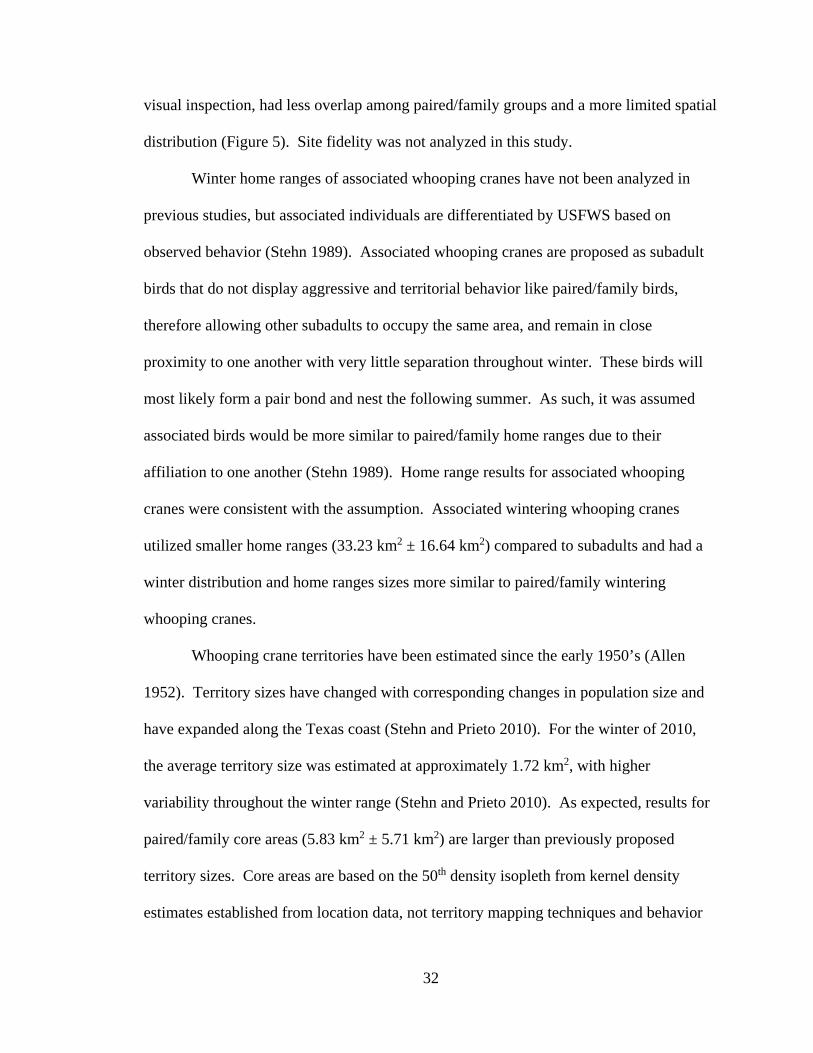
32

visual inspection, had less overlap among paired/family groups and a more limited spatial

distribution (Figure 5). Site fidelity was not analyzed in this study.

Winter home ranges of associated whooping cranes have not been analyzed in

previous studies, but associated individuals are differentiated by USFWS based on

observed behavior (Stehn 1989). Associated whooping cranes are proposed as subadult

birds that do not display aggressive and territorial behavior like paired/family birds,

therefore allowing other subadults to occupy the same area, and remain in close

proximity to one another with very little separation throughout winter. These birds will

most likely form a pair bond and nest the following summer. As such, it was assumed

associated birds would be more similar to paired/family home ranges due to their

affiliation to one another (Stehn 1989). Home range results for associated whooping

cranes were consistent with the assumption. Associated wintering whooping cranes

utilized smaller home ranges (33.23 km2 ± 16.64 km2) compared to subadults and had a

winter distribution and home ranges sizes more similar to paired/family wintering

whooping cranes.

Whooping crane territories have been estimated since the early 1950’s (Allen

1952). Territory sizes have changed with corresponding changes in population size and

have expanded along the Texas coast (Stehn and Prieto 2010). For the winter of 2010,

the average territory size was estimated at approximately 1.72 km2, with higher

variability throughout the winter range (Stehn and Prieto 2010). As expected, results for

paired/family core areas (5.83 km2 ± 5.71 km2) are larger than previously proposed

territory sizes. Core areas are based on the 50th density isopleth from kernel density

estimates established from location data, not territory mapping techniques and behavior

33

observed in the field. Furthermore, 50th density isopleths are proposed to overestimate

core areas (Wilson et al. 2010). However, these results confirm smaller areas are being

utilized more intensely compared to the surrounding home range (21.77 km2 ± 22.24

km2), and based on visual observation, less overlap occurs between core areas than home

ranges for all three age-classes (Figure 5). In addition, core areas developed for the

winter of 1988-1989 align well with mapped territories from the winter of 1990-1991

(Stehn and Prieto 2010). The alignment of core areas developed from kernel density

estimators with previously mapped territories suggests the results are consistent with

observed whooping crane wintering distribution and behavior. Thus, these results may be

used to construct improved resource selection studies in the future.

The similarity between associated and paired/family whooping crane home range

sizes and overall spatial extent and their dissimilarity with subadult whooping crane

home ranges suggests age-class is an important factor influencing wintering whooping

crane space-use patterns. Therefore, distinguishing between age-classes is crucial for

future habitat and spatial modeling studies.

The best model to explain variation among wintering whooping crane home

ranges included only landscape metrics: barren, grassland, live oak, marsh, water, and

Simpson’s diversity index (Model m247; Table 6). Previous studies have suggested

population density pressure and wintering location as potential factors influencing

wintering whooping crane space-use patterns (Stehn and Prieto 2010). Based on results

from the regression, these factors were non-influential suggesting whooping crane home

range sizes are primarily defined by habitat composition and that wintering whooping

cranes are dependent upon a variety of habitats during the winter season. However, it is

34

important to note that the AWBP was estimated to equal 138 individuals (USFWS,

unpublished data) compared to over 500 individuals estimated for the winter of 2017-

2018 (Butler and Harrell 2018). In the winter of 1988-1989 there may not have been a

large enough population to capture influences of population density pressure on space-

use by wintering whooping cranes. Birds would have been able to distribute relatively

widely, potentially allowing habitat and food resources to be key factors driving their

spatial extent on the wintering grounds. The whooping crane winter range consists of a

mosaic of habitats from open bays and estuaries to tidal flats and salt marshes, as well as

live oak and crop land in the uplands (Stehn and Prieto 2010; Smith et al. 2014). The

birds primarily occur adjacent to or within water areas for feeding and utilize different

methods of foraging depending on the type of prey or food item (Allen 1952).

Dominant food items include blue crabs, razor clams, wolfberry, fiddler crabs,

plicate horn shells, other snails, shrimp, crayfish, and acorns (Chavez-Ramirez 1996).

Blue crabs and wolfberries are their primary food items when tidal flats are flooded

whereas clams are the predominant food item when tides and associated water depths are

low (U.S. Fish and Wildlife Service 1994). The number of factors in the best-fit model

reflects the importance of various land cover types to wintering whooping cranes. The

complexity of tides, salinity fluxes, and habitats drive variation in the winter food supply

for whooping cranes resulting in the need of a variety of land cover types. Model

averaging results for wintering whooping crane core areas were consistent with previous

descriptions of landscape composition within territories (Bonds 2000; Stehn and Prieto

2010). Bonds (2000) and Stehn and Prieto (2010) suggested the dominance or percentage

of salt marsh within a territory largely influences wintering whooping crane space-use,

35

though it may not be the only factor. Based on these results, winter whooping crane core

area size increased with a decrease in salt marsh composition (Table 6). This suggests a

negative relationship between salt marsh composition and core area size.

Results suggest a positive relationship between core area size and habitat diversity

(Table 6); i.e. core area size increases with an increase in habitat diversity. This result is

consistent with the resource dispersion hypothesis (RDH; Macdonald 1983). As

resources are more distributed across the landscape, resulting in patches of resources, a

larger home range is formed to account for the increased dispersion required. As

previously stated, salt marsh has been proposed as a critical land cover type for wintering

whooping cranes and based on our previous results, influences core area size. However,

these additional model averaging results imply core area size is also dependent upon

habitat diversity. Similar to home ranges, multiple land cover types comprise the core

area of wintering whooping cranes and play a factor in its overall size.

Although whooping crane core areas are influenced by the abundance of salt

marsh, this one habitat type cannot intrinsically define core area size. In this study, core

areas were used as a proxy for territories. The accuracy of core area size compared to

previously delineated territories (Stehn and Prieto 2010) was not of concern, as core area

estimators will overestimate territory size, but instead focused on the estimated home

ranges and core areas being ‘true’; e.g., spatially accurate on the landscape (Borger et al.

2006). Based on the literature and current knowledge of wintering whooping cranes, the

developed kernel density estimators provided biologically relevant home ranges and core

areas from USFWS aerial census point locations. However, conclusions from these

results should also consider potential discrepancies that arise from comparing space-use

36

based on point location collected in 1988-1989 with a more recent land cover dataset

(TPWD TESD 2013). Relative sea-level rise within the study area (Rockport, Texas) has

risen a rate of 4.66 mm/year (0.18 in/year) since 1948 resulting in changes to the

landscape as more areas become inundated and waves and other erosive energy move

inland (Montagna et al. 2007). Therefore, the percent of land cover types occupied by

wintering whooping cranes in 1988-1989 differs to some degree from those identified in

this analysis using TPWD’s TESD (2013). Future analysis of whooping crane space-use

should consider either the use of historical imagery in conjunction with the historic, long-

term whooping crane location dataset, or the use of more recent land cover databases

along with recently collected telemetry data (Dr. Wade Harrell, Whooping Crane

Coordinator, USFWS, pers. Comm.).

Management Implications

Results provide further insight concerning the spatial distribution of wintering

whooping cranes along the Texas coast, and contribute to the identification of, and future

protection of, potential wintering whooping crane habitat. The spatial distribution of

wildlife populations is influenced by both biotic and abiotic factors. This study differs

from most by not limiting our analysis to a single factor or a limited number of factors to

describe a population’s spatial distribution (Schradin et al. 2010; van Beest et al. 2011).

The breeding ground used by the AWBP flock is primarily within a protected

national park and is remote relative to human disturbance, thus not anticipated as a

potential liming factor (Tischendorf 2004). Within the wintering ground, the majority of

habitat used currently by wintering whooping cranes is located within a federally

protected national refuge. However, an increasing proportion of winter habitat is within

37

private land that has high human disturbance potential, such as planned subdivisions,

road expansions, and development of canals. Moreover, any future winter range

expansion, if predicted at this time with current conservation strategies, would primarily

occur within private land along the Texas coast. Consequently, the winter ground was

proposed as a limiting factor influencing the potential growth of the AWBP population

size (Stehn and Prieto 2010; Gil-Weir et al. 2012).

Based on the results, land management decisions and conservation strategies for

wintering whooping crane should be developed with an emphasis on subadults and

paired/family individuals as uniquely distinct groups utilizing similar habitat types, but at

significantly different quantities and spatial extents. The developed home range

estimates provide the first quantitative analysis of space-use strategies by wintering

subadult whooping cranes. Results concluded that subadults have widely-distributed

home ranges across multiple habitat types within the winter range; whereas paired/family

birds have smaller home ranges and utilize core areas dependent upon the quantity of salt

marsh and habitat diversity. To develop conservation strategies or land management

plans with these two groups combined as one could lead to insufficient results. For

example, human development within the winter range could influence subadults and

paired/family whooping cranes differently, depending on the location, intensity, and

spatial extent of the development. Because subadults traverse a larger area than

paired/family individuals, and do not display prominent site fidelity to a territory, they

may be able to adapt to development if other suitable habitat types are available within a

certain distance.

38

In contrast, development may severely affect paired/family individuals.

Paired/family whooping cranes may remain in a territory despite human degradation,

resulting in a territory that is no longer meeting their energetic needs and potentially in

decreased reproductive success or survivorship. By incorporating home range and core

areas of subadult and paired/family whooping cranes, land management and protection

strategies can plan more appropriately for which habitat types and at what extent they

will most likely be used by wintering whooping cranes.

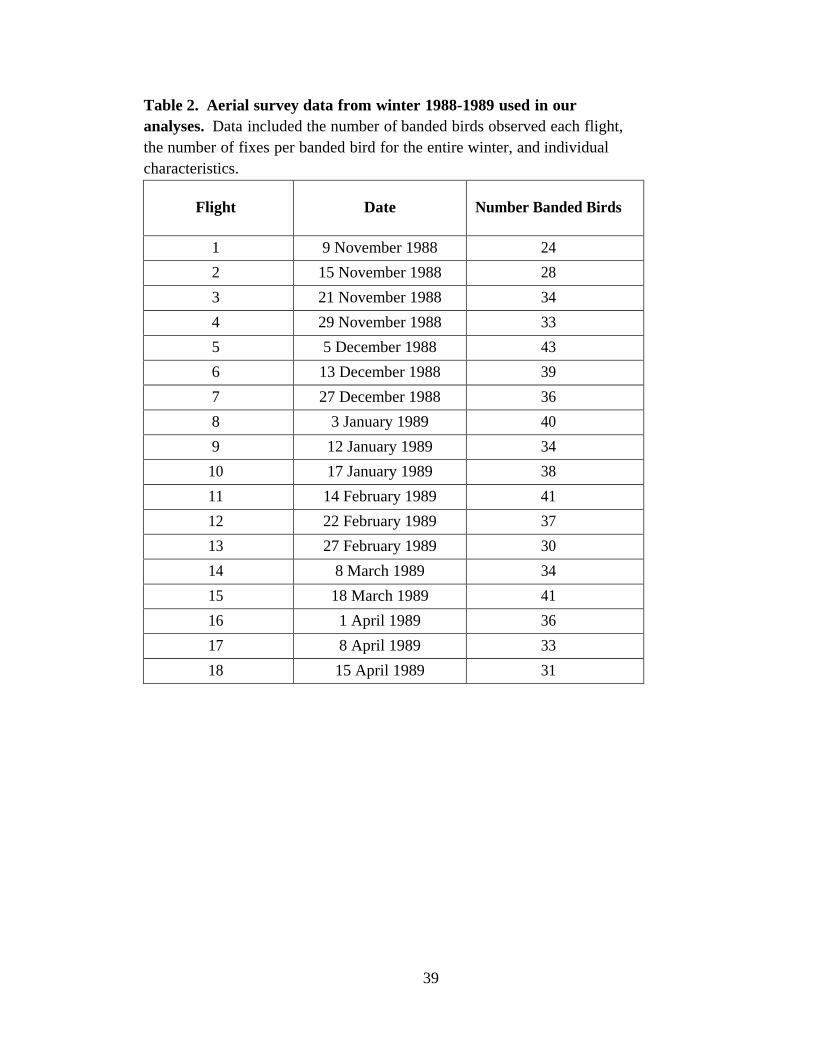
39

Table 2. Aerial survey data from winter 1988-1989 used in our analyses. Data included the number of banded birds observed each flight, the number of fixes per banded bird for the entire winter, and individual characteristics.

Flight Date Number Banded Birds

1 9 November 1988 24 2 15 November 1988 28 3 21 November 1988 34 4 29 November 1988 33 5 5 December 1988 43 6 13 December 1988 39 7 27 December 1988 36 8 3 January 1989 40 9 12 January 1989 34 10 17 January 1989 38 11 14 February 1989 41 12 22 February 1989 37 13 27 February 1989 30 14 8 March 1989 34 15 18 March 1989 41 16 1 April 1989 36 17 8 April 1989 33 18 15 April 1989 31

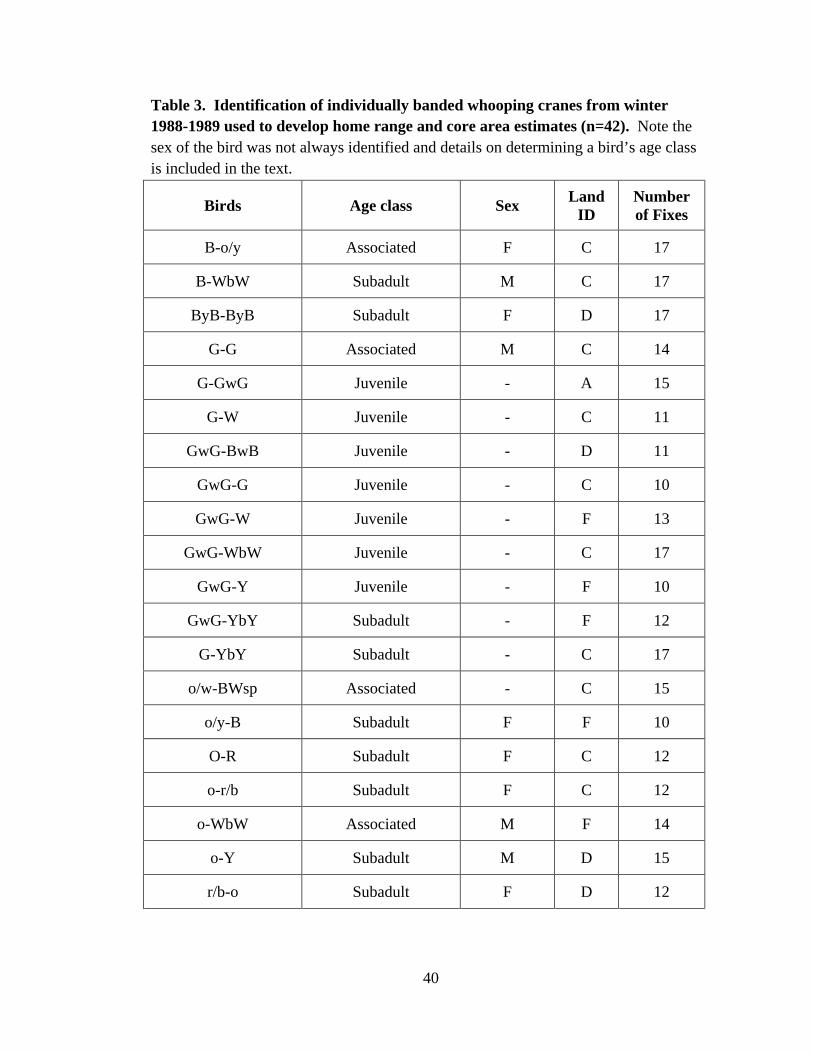
40

Table 3. Identification of individually banded whooping cranes from winter 1988-1989 used to develop home range and core area estimates (n=42). Note the sex of the bird was not always identified and details on determining a bird’s age class is included in the text.

Birds Age class Sex Land ID

Number of Fixes

B-o/y Associated F C 17

B-WbW Subadult M C 17

ByB-ByB Subadult F D 17

G-G Associated M C 14

G-GwG Juvenile - A 15

G-W Juvenile - C 11

GwG-BwB Juvenile - D 11

GwG-G Juvenile - C 10

GwG-W Juvenile - F 13

GwG-WbW Juvenile - C 17

GwG-Y Juvenile - F 10

GwG-YbY Subadult - F 12

G-YbY Subadult - C 17

o/w-BWsp Associated - C 15

o/y-B Subadult F F 10

O-R Subadult F C 12

o-r/b Subadult F C 12

o-WbW Associated M F 14

o-Y Subadult M D 15

r/b-o Subadult F D 12

41

Table 3. Continued.

Birds Age class Sex Land ID

Number of Fixes

R-G Juvenile - C 14

R-GwG Juvenile - C 14

r-r Juvenile - C 11

RwR-BwB Juvenile - A 10

RwR-GwG Juvenile - C 16

RwR-YbY Associated - C 14

R-Y Associated - E 13

R-YbY Associated - C 17

W-B Adult F F 10

WbW-GwG Juvenile - C 15

WbW-WbW Paired F F 18

W-G Subadult F F 19

W-RWR Associated M C 13

y/b-o Paired F C 12

Y-b/b Paired M D 12

YbY-G Subadult - C 12

YbY-o Associated - C 12

YbY-RwR Associated - F 14

YbY-W Subadult - D 15

YbY-Y Subadult - F 10

YbY-YbY Subadult - C 18

Y-Y Associated F E 14

Y-YbY Subadult - F 19

42

Table 4. Land cover types located within winter whooping crane home ranges. Land cover types were grouped and reduced from twenty five detailed types to nine more generalized land cover types. Land cover types highlighted in grey were determined to be dominant land cover types in winter whooping crane home ranges based on area > 1km2 within home range.

Common Name1 Land Use / Land Cover1

Reclassified Land Use/Land Cover

Coastal: Tidal Flat 1 Barren

Post Oak Savanna: Live Oak Motte and Woodland 3 Live Oak

Coastal Bend: Floodplain Live Oak Forest 3 Palustrine Woodland

Coastal Bend: Riparian Live Oak Forest 3 Mixed Shrub

Post Oak Savanna: Post Oak Motte and Woodland 5 Upland Woodland

Coastal Bend: Floodplain Hardwood Forest 5 Palustrine Woodland

Coastal Bend: Riparian Hardwood Forest 5 Palustrine Woodland

Gulf Coast: Salty Prairie Shrubland 7 Mixed Shrub

Coastal Bend: Floodplain Deciduous Shrubland 7 Mixed Shrub

Coastal Bend: Riparian Deciduous Shrubland 7 Mixed Shrub

Gulf Coast: Salty Prairie 9 Grassland

Post Oak Savanna: Live Oak Shrubland 11 Upland Shrub

Coastal Bend: Floodplain Evergreen Shrubland 11 Mixed Shrub

Coastal Bend: Riparian Evergreen Shrubland 11 Mixed Shrub

Coastal: Sea Ox-eye Daisy Flats 11 Mixed Shrub

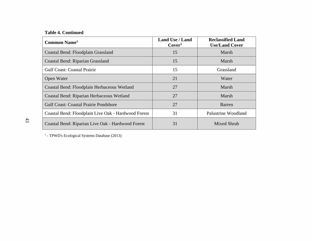
43

Table 4. Continued

Common Name1 Land Use / Land Cover1

Reclassified Land Use/Land Cover

Coastal Bend: Floodplain Grassland 15 Marsh

Coastal Bend: Riparian Grassland 15 Marsh

Gulf Coast: Coastal Prairie 15 Grassland

Open Water 21 Water

Coastal Bend: Floodplain Herbaceous Wetland 27 Marsh

Coastal Bend: Riparian Herbaceous Wetland 27 Marsh

Gulf Coast: Coastal Prairie Pondshore 27 Barren

Coastal Bend: Floodplain Live Oak - Hardwood Forest 31 Palustrine Woodland

Coastal Bend: Riparian Live Oak - Hardwood Forest 31 Mixed Shrub

1 - TPWD's Ecological Systems Database (2013)

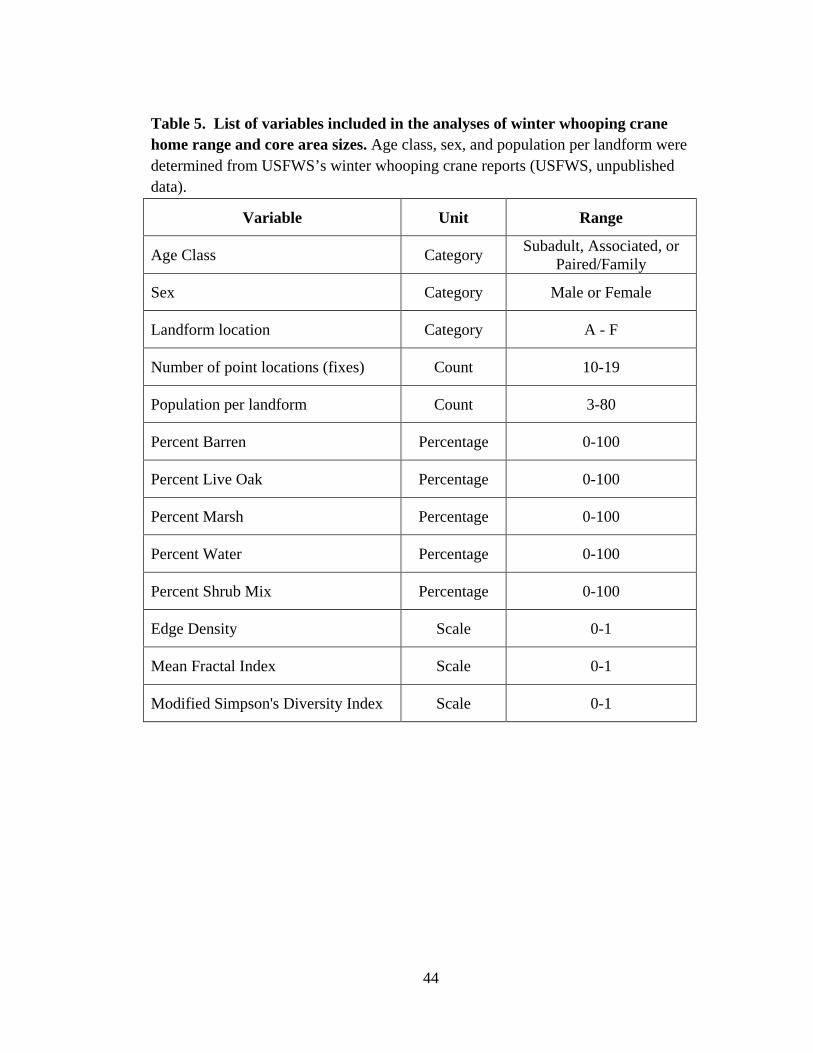
44

Table 5. List of variables included in the analyses of winter whooping crane home range and core area sizes. Age class, sex, and population per landform were determined from USFWS’s winter whooping crane reports (USFWS, unpublished data).

Variable Unit Range

Age Class Category Subadult, Associated, or Paired/Family

Sex Category Male or Female

Landform location Category A - F

Number of point locations (fixes) Count 10-19

Population per landform Count 3-80

Percent Barren Percentage 0-100

Percent Live Oak Percentage 0-100

Percent Marsh Percentage 0-100

Percent Water Percentage 0-100

Percent Shrub Mix Percentage 0-100

Edge Density Scale 0-1

Mean Fractal Index Scale 0-1

Modified Simpson's Diversity Index Scale 0-1

45

Table 6. Set of selected models developed to estimate key variables influencing home range and core area sizes of wintering whooping cranes. Note only five models for home ranges and core areas are shown.

Model Terms K AICc AICc wi m247 HR~Barren+Grass+Oak+Marsh+Water+MSIDI 7 25.20 0.00 0.85 m257 HR~Water+Shrub+ED+MFI+MSIDI 7 31.00 5.86 0.05 m211 HR~Water+Shrub+ED+MSIDI 6 32.71 7.51 0.02 m280 HR~Landpop+Barren+Grass+Oak+Marsh+Shrub 8 33.50 8.38 0.01 m252 HR~Oak+Marsh+Water+Shrub+ED 7 33.80 8.62 0.01 ca8 CA~Marsh 3 12.20 0.00 0.14 ca59 CA~Oak+Marsh 4 12.50 0.30 0.12 ca79 CA~MFI+MSIDI 4 12.80 0.58 0.10 ca68 CA~Marsh+MFI 4 13.60 1.43 0.07 ca46 CA~Barren+Marsh 4 14.00 1.80 0.06

- Response variable = log-transformed home range size (HR) and log tranformed core area size (CA) - Potential predictor variables = age class, location (location ID), number of fixes, landform population (Landpop), barren, grassland (grass), liveoak (oak), marsh, water, shrubmix (shrub), edge density (ED), mean fractal index (MFI), and modified Simpson’s diversity index (MSIDI) - Only 5 modelsmodel presented out of 224 home range and 185 core area models

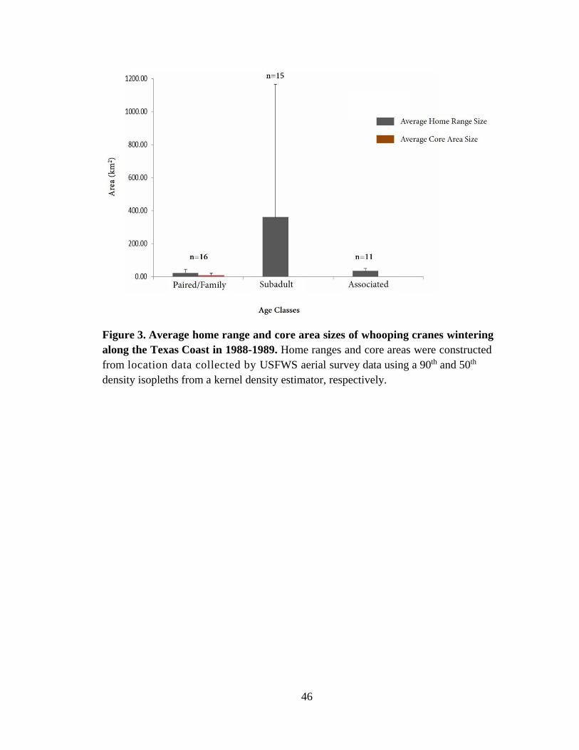
46

Figure 3. Average home range and core area sizes of whooping cranes wintering along the Texas Coast in 1988-1989. Home ranges and core areas were constructed from location data collected by USFWS aerial survey data using a 90th and 50th density isopleths from a kernel density estimator, respectively.

47

Figure 4. Home ranges and distribution of subadult (top) and paired/family (bottom) whooping cranes within the winter range along the Texas coast in 1988-1989. Home ranges were constructed using a 90th density isopleth from a kernel demsity estimator (Geospatial Modelling Environmental [GME] Software and ArcMap 10.1).

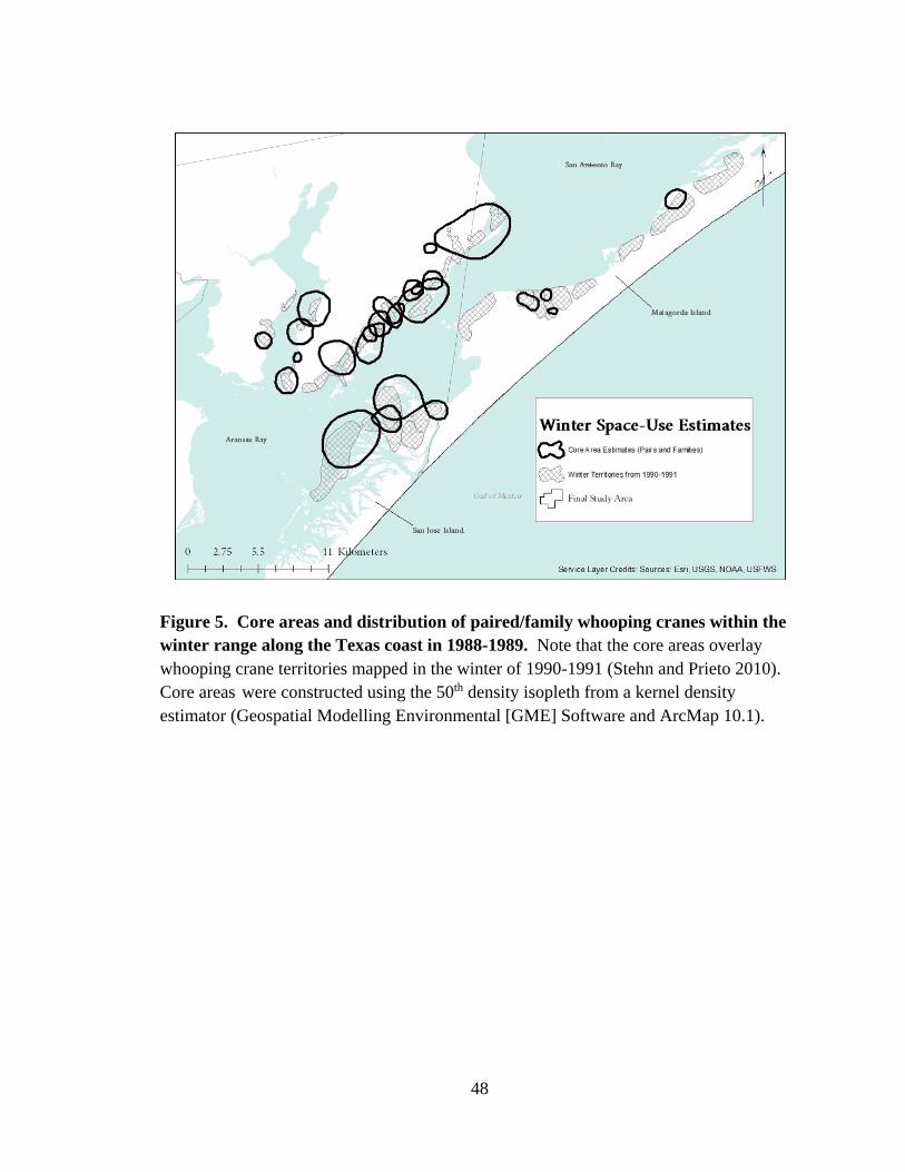
48

Figure 5. Core areas and distribution of paired/family whooping cranes within the winter range along the Texas coast in 1988-1989. Note that the core areas overlay whooping crane territories mapped in the winter of 1990-1991 (Stehn and Prieto 2010). Core areas were constructed using the 50th density isopleth from a kernel density estimator (Geospatial Modelling Environmental [GME] Software and ArcMap 10.1).

49

III. WINTER WHOOPING CRANE DISTRIBUTION MODEL ALONG

THE TEXAS COAST

To further evaluate winter habitat used by whooping cranes, a species distribution

model (SDM) for the AWBP was developed using the same long-term whooping crane

location dataset from the previous chapter. Wildlife biologists use SDMs to relate the

location or occurrence of a target species with influential environmental and spatial

characteristics and predict the presence of a species based on the estimated suitability.

Similar models in the literature include habitat suitability models (HSMs), ecological

niche models, and resource selection functions (RSFs). Each of these models focus on

the same ecological question as a SDM, what is the current and potential spatial

distribution of a species (Bradley et al. 2012; Elith and Leathwick 2009; Elith et al. 2011;

Franklin 2010 Manly et al. 2002)? Species distribution models have been used to explain

the present, and predict the future spatial distribution of sessile (stiff sedge (Carex

bigelowii [Pearson and Dawson 2003); cheatgrass (Bromus tectorum L.) [West et al.

2015]) and mobile (black storks (Ciconia nigra) [Jiguet et al. 2011]; brown bear (Ursus

arctos) [Gils et al. 2014]; goitered gazelle (Gazella sugutturosa) [Khosravi et al. 2015];

puma (Puma concoloro) [Angelieri et al. 2016]; clapper rail (Rallus crepitans) [Roach et

al. 2017]) species based on key ecological drivers, such as climate, elevation, soil,

vegetation, human disturbance, etc. Therefore, results from SDM can provide essential

insight for conservation planning and resource management for the target species (Elith

and Leathwick 2009).

One of the alternative criteria outlined in the recent international whooping crane

recovery plan (CWS and USFWS 2007) is for the AWBP to be self-sustaining and

50

remain above 1,000 individuals including 250 reproductive pairs. As of the winter of

2017-2018, the AWBP consists of approximately 505 individuals (Butler and Harrell

2018) distributed over approximately 9,000 ha (22,240 acres) along the Texas coast

(CWS and USFWS 2007). Therefore, an important objective in the recovery plan for the

endangered whooping crane is to identify suitable habitat and determine availability of

this habitat for a growing population. A SDM for wintering whooping cranes was

developed using maximum entropy software (Maxent v. 3.3.3 k) (Phillips et al. 2006;

Maxent 2011) to identify highly suitable habitat within the wintering grounds. I

developed.

Maxent is a freely available software that uses the most uniform distribution

(maximum entropy) of sample locations for a target species and compares them to a set

of background locations based on constraints derived from the data to estimate the

probability of distribution (Baldwin 2009; Phillips et al. 2006). Inputs to the model

include presence-only data and environmental data determined a priori to be potentially

significant factors influencing the ecology of the target species. Results from Maxent

include raw, cumulative, and logistic output data that can be presented and interpreted as

a projection in a geographic information system (GIS) (Baldwin 2009). In ArcMap, the

logistic data is interpreted as a probability of occurrence as predicted from the

environmental variables (Baldwin 2009) or can be interpreted as an indication that a

given area could support the presence or absence of the target species based on defined

thresholds (Baldwin and Bender 2008; Sheehan et al. 2016; Thorn et al. 2009).

GIS-derived data layers, such as distance from select features, percent vegetative

cover, and density of select features, have shown to provide additional ecological

51

explanation in species distribution models, including SDMs derived from Maxent

(Angelieri et al. 2016; Buckman-Sewald et al. 2014; Gils et al. 2014; Sheehan et al.

2016). In this chapter, thirty-five ecological and environmental data layers were

determined a priori to be explanatory variables and were used to develop winter

whooping crane species distribution models. This is the first study to develop a winter

whooping crane species distribution model using GIS-derived ecological and

environmental variables in Maxent. The purpose of this study is to derive GIS-layers of

relevant ecological and environmental data layers and evaluation their influence on the

AWBP winter distribution, develop a species distribution model for wintering whooping

cranes along the Texas coast, and identify suitable habitat outside the current winter

range for habitat conservation measures.

Methods

The long-term wintering whooping crane location data from the USFWS detailed

in Chapter 2 was used to develop the winter whooping crane species distribution models.

The geographic extent of whooping cranes location from the long-term dataset was used

to determine the study area, background extent in Maxent, and develop ecological and

environmental data layers in ArcMap. Details on the ecological and environmental data

layers used in ArcMap are included below and outlined in Appendix A.

Whooping Crane Data

As described in the previous chapter, locations of wintering whooping cranes

have been recorded regularly by the USFWS since 1950, providing an extensive long-

term dataset of the last wild-flock of the federally endangered whooping crane population

(Stehn and Taylor 2008). The dataset has been determined to be presence-only data

52

because of the sample design of the aerial transects and sample locations were assumed

sub-samples of the population as the transect-aerial survey method may have failed to

detect the entire population at any given time (Strobel and Butler 2014). Additional

information regarding winter aerial surveys from 1950 to 2011 is provided on the U.S.

Fish and Wildlife Service’s Aransas National Wildlife Refuge website (USFWS 2016)

and in Taylor et al. (2015).

The long-term location dataset was reduced to data from flights conducted

between the winters of 1982-1983 and 2010-2011 (n=26,239) using ArcMap 10.1. It was

further reduced to locations recorded by the same USFWS investigator to reduce sample

bias that may occur among multiple observers (n=24,233) and to locations obtained

between the winter months of November 7 to April 17 (n=22,883). Since timing of

migration influences how individual whooping cranes may utilize habitat on the

wintering grounds (Stehn and Johnson 1987; Stehn and Prieto 2010), the dataset was

limited to data points from days between these dates to coincide with high population

numbers arriving during fall migration and departing during spring migration (LaFever

2006). Locations within these dates also reduce the number of unusual use of still vacant

territories when the full population has not arrived on the wintering grounds from

migration (Stehn 1992) and captures locations influenced by territorial defense behavior

(LaFever 2006). Additional data reduction limited location data to only winters from

2004-2005 to 2009-2010 (n=5,842). Data from winters prior to 2004-2005 were removed

in order to meet the limitations of environmental data derived from recent, freely

available datasets, such as recent land cover datasets. Lastly, all locations with the

attribute of ‘unknown location’ were removed (n=5,784).

53

Determining Study Area Extent

The overall geographical extent used as input to Maxent is termed the

‘background’, and is essential to how the algorithm develops species distribution

estimates. A background with an extent too small or too large can result in under- and

over-estimating the potential distribution of a target species, respectively. Maxent creates

pseudo-absences based on the input location data (presence-only) and background extent.

If the background extent is too large, it will include environmental variables that are

irrelevant for the sample population, which will result in skewed and uninformative

results (Elith et al. 2011). For this study, the initial background extent was developed by

buffering each location point by a radius of 50 km. However, it was determined this

background extent was too small based on the similarity of environmental conditions in

the surrounding areas that could be support suitable winter whooping crane habitat.

Therefore, the final background extent was increased in order to include areas determined

to be potentially suitable for wintering whooping cranes by local stakeholders, such as

marsh within East Matagorda Bay and the Nueces Delta (Dr. Elizabeth Smith, Senior

Whooping Scientist, International Crane Foundation, pers. comm.).

The final extent was created from a 100-km buffer created around each whooping

crane data point that was then adjusted in ArcMap to align with spatial extent of specific

environmental parameters. Using U.S. Geological Survey (USGS)-defined sub-basins,

the most northeastern boundary of the final background extent was clipped to the East

Matagorda Bay and San Bernard Sub-basins and the southwestern boundary was clipped

to the South Corpus Christi Bay and North Laguna Madre Sub-basins. The northwestern

boundary (inland) was limited to the West Gulf Coastal Plain Region identified in the

54

Texas Parks and Wildlife Department’s Ecological Mapping System of Texas (EMST)

database, which also aligns with their historic distribution along the Texas coast (Allen

1952). The southwestern boundary of the final extent was restricted to the edge of the

Gulf of Mexico (Figure 6).

Ecological and Environmental Data Layers

A number of available land cover datasets were considered such as the National

Agricultural Imagery Program (NAIP), National Land Cover Dataset (NLCD; USGS

NLCD 2006), and TPWD EMST (2004)) for the base habitat layer for model

development. These datasets were determined to be unsuitable due to scale and accuracy

limitations. The existing Composite Habitat Type Dataset (CHTD; Smith et al. 2014)

comprised of the TPWD EMST (10-m resolution), Benthic Habitat Atlas (BHA; 10-m

resolution) from the National Oceanic and Atmospheric Association (NOAA BHA 2007),

and the National Wetland Inventory (NWI; resolution varies from sub-meter to meters)

from USFWS (2016) was modified and extended for use in the winter whooping crane

species distribution model (Figure 7). The CHTD was modified to include an updated

TPWD EMST and extended the geographic extent to encompass the Matagorda Bay

system in the north and the Corpus Christi Bay system in the south. Modification steps

followed the classification methods used in Lumb (2014) and Smith et al. (2014) to

process the spatial land cover data to derive the same 33 mesohabitat classes. These

classes were subsequently reclassified into 16 classes considered applicable to wintering

whooping cranes (Table 7). These 16 classes were subsequently used to derive 26 of the

36 input layers in Maxent to develop the wintering whooping crane distribution model, as

described below (Table 8).

55

Climate Data. Worldclim data (Hijmans et al. 2005) at a resolution of 1 km2 is

commonly used to guide species distribution models in Maxent (Gils et al. 2014;

Gschweng et al. 2012). Since species distribution models require all data layers to be in

the same resolution use of Worldclim data for temperature and precipitation would

require all other data layers to be resampled to a resolution of 1-km2. In doing so,

environmental complexity of the study area would be reduced, most likely resulting in an

oversimplified, less informative estimate of wintering whooping crane distribution.

Therefore, climate data was not included in development of the SDMs. Climate was

assumed to be relatively similar across the study area due to small size of the study area.

However, future modeling across a larger extent should consider influences from

temperature and precipitation.

Soil Data. Soils play an important role in the type of vegetation present within a

given area, and to some extent, the overall ecosystem. A hydric soil layer was derived

from U.S. Department of Agriculture (USDA) Natural Resources Conservation Services’

(NRCS) soil data (SSURGO) (Soil Survey Staff, USDA, NRCS 2016). The soil layer

included four classes: hydric soil, non-hydric soil, other (all remaining soil classes), and

water (Figure 8). These classes were based on the USDA NRCS’s National Hydric Soils

List for the state of Texas (USDA NRCS 2017).

Salinity Data. The Texas Water Development Board (TWDB) has validated the

use of a 2-dimensional hydrodynamic model known as TxBLEND to determine water

velocity, surface elevation, and salinity levels within all seven major estuaries in the state

of Texas (Guthrie et al. 2010a [Upper Guadalupe]; Guthrie et al. 2010b [Guadalupe and

Mission-Aransas Estuaries]; Schoenbaechler et al. 2011a [Nueces Estuary];

56

Schoenbaechler et al. 2011b [Laguna Madre Estuary]; Schoenbaechler et al. 2011c

[Lavaca-Colorado Estuary and East Matagorda Bay]). TWDB provided TxBLEND daily

and monthly salinity data from the 5-Bay Model, which includes bays and estuaries

between Corpus Christi Bay to Matagorda Bay, and the Matagorda Model for just East

Matagorda Bay. Data coincides with individual, georeferenced nodes that are part of the

model grid established by TWDB. The 5-Bay Model included 8,595 nodes, and the East

Matagorda Bay area included 8,340 nodes.

Node data were reduced by removing nodes with incomplete data for the entire

timeframe between the winter of 2004-2005 to 2009-2010 (5-Bay model = 8,533 [-62

nodes] and East Matagorda = 8,309 [-31 nodes]), were converted to spatial data layers in

ArcMap, and merged into one salinity dataset (Figure 9). Average, maximum, and

minimum salinities between winters of 2004-2005 to 2009-2010 were calculated at each

node. Average and minimum salinity were calculated without values of zero. Salinity

values for all years ranged from 0.01 ppt to 38.47 ppt for the 5-Bay TWDB and 0.01 ppt

to 33.39 ppt for East Matagorda Bay.

Ordinary kriging method in ArcMap was then used to develop continuous salinity

data layers. Kriging is a statistical method that interpolates data across a given distance

by relating known values in one location with unknown values in other areas. Average,

maximum, and minimum salinities for each year from winters 2003-2004 to 2009-2010

were interpolated across the extent the study area, including marine, estuarine, palustrine,

and upland habitat types identified in the CHTDv2. Initially, interpolated salinities were

limited to just the marine and estuarine classes; however, limiting salinities to just marine

and estuarine classes oversimplifies the effect salinity may have on the distribution of

57

wintering whooping cranes across the full landscape, especially during extreme

conditions. Salinities are assumed to increase within palustrine classes, such as ponds

located inland from marine and estuarine classes. Therefore, it is important to include

salinities further inland from marine and estuarine habitat types in determining suitability

for wintering whooping cranes.

To develop a reasonable estimate of salinities within more inland habitat types, an

‘inundation polygon’ was created for the maximum extent of inland inundation using an

approach similar to a method derived by Lumb (2014). Lumb (2014) used results from

the Sea, Lake, and Overland Surges from Hurricanes (SLOSH) model developed by the

National Weather Service (Jelesnianski et al., 1992) to develop an inland study area

boundary based on inland inundation. The SLOSH model estimates storm surge heights

for hurricanes based on atmospheric pressure, size, forward speed, and track data.

Results depend on the model parameters, including the intensity of the modeled hurricane

(Category 1 – 5), and where the hurricane hits land. The maximum extents of inland

inundation within the study area was estimated using worst-case scenarios modeled for a

Category 5 storm hitting Corpus Christi, Matagorda, and Galveston Bays during high tide

(Lumb 2014).

Maximum of the Maximum Envelope of High Water (MOM product) for a

category 5 hurricane striking major bays within the study area at high tide were

downloaded (National Weather Service Meteorological Development Laboratory,

registration required). MOM products combine the highest storm surge values for all

hypothetical hurricanes for each potential storm category within a selected SLOSH model

basin at mean and high tide and represent the worst-case scenario for a given category of

58

a storm under “perfect” storm conditions. For this study, MOM products for category 5

storms hitting Corpus Christi Bay, Matagorda Bay, and Galveston Bay SLOSH basins at

high tide were utilized. The MOM vector grids were imported into ArcMap 10.1 (Hurler

et al., 2015; NOAA CSC 2012) to develop the ‘inundation polygon’ (similar to Lumb,

2014). The inundation polygon was created by removing ‘dry points’ or areas with ‘no

data’ values; i.e., all Category 5 at high tide (C5_high) values below 99.9, and data

outside the study area extent. The MOM SLOSH data was converted from feet to meters

and converted to points in order to interpolate storm surge water surface values across the

entire study area using an inverse distance weighting (IDW) interpolation.

Inundation (depth and horizontal extent) was calculated by subtracting land

surface elevations provided by a mosaicked Digital Elevation Model (DEM) (detailed

below) from the interpolated storm surge water surface values. The created inundation

vectors (polygon) for Corpus Christi, Matagorda, and Galveston Bays were examined in

ArcMap, and inundation values from the most inland extents were merged to form a final

‘inundation layer’. The final ‘inundation layer’ was used to mask the interpolated

salinities (average, maximum, and minimum) across the entire study area, and limit

salinities to areas inland from the bays and estuaries based on modeled inundation for

worst-case scenarios (Figure 10). The created salinity raster was based on interpolated

data.

A vertical datum shift of the interpolated water surfaces was not calculated

(NOAA CSC 2012). The purpose of the ‘inundation layer’ was to estimate the farthest

inland extent of storm inundation under the worst-case scenario conditions. A datum

shift uses surface elevations from nearby tide gauges to improve the accuracy of

59

interpolated water surfaces. Future investigations related to the effects of sea-level rise

and local subsidence using the created ‘inundation layer’ are recommended to incorporate

transformation of the vertical datum to local tide gauges.

Derived Data Layers. The revised mesohabitat land cover layer was used in

conjunction with additional spatial datasets (see Appendix A) to create additional

ecological and environmental input data layers in Maxent determined a priori to be

factors influencing wintering whooping crane distribution. These layers included

elevation, slope, roughness, percentage of habitat types, distances to landscape features,

density of roads, and calculated landscape composition and configuration (Table 8). All

layers were rasterized in ArcMap to a 30-meter grid, set to the same spatial extent, and

were projected to a common spatial reference (NAD 1983 Texas Centric Albers Equal

Area [EPSG:3085]).

Some environmental layers, as detailed below, were calculated using a search

radius of 2.98 km, which is the radius of the largest whooping crane territory on the

winter grounds (1,191 ha [Stehn and Prieto 2010]). This radius was determined to be

reflective of areas potentially more influential on wintering whooping cranes. Whooping

cranes spend the majority of daytime (approximately 63 to 66%) foraging on the winter

grounds, which results in continuous walking in search of food (Chavez-Ramirez 1996;

LaFever 2006). Therefore, for some environmental layers, such as density of roads,

patches within the search radius are most likely influencing suitability of habitat to a

whooping crane more than those patches farther away. Multiple suitability models and

species distribution models incorporate the proportion of different vegetative and

topographic variables within a specific distance surrounding the sample location.

60

Moreover, specific distances are often derived from the radius of the targeted species’

home range (Latif et al. 2015; Timoney 1999), the minimum distance capable for

detection (Stralberg et al. 2010), daily distance traveled (Coates et al. 2014), and the

maximum distance habitat selection was observed from a nest for similar species

(Timoney 1999).

Euclidean distance tool in ArcMap was used to calculated distance to landscape

features as noted in Table 7. In addition, four raster layers were derived from the

mesohabitat land cover layer using Fragstats (McGarigal et al. 2012) with an 8-cell

neighborhood rule (Roach et al. 2017). These included edge contrast (ECON) (percent of

maximum contrast between two patches), patch area (PA), patch shape or contiguity

index (CONTIG), and patch aggregation or proximity index (PROX). The proximity

index was limited to a 2.98-kmsearch radius. The generated spatial metrics were

imported into ArcMap and saved as raster for use in future analyses.

The edge-contrast analysis included a 50-meter landscape border and an edge-

contrast table. The border includes all patches within a pre-determined amount of land

(50-m) surrounding the study area and each border patch is set to the negative of the

patch type. Patches within the border provide information on patch type adjacency for

patch on the edge of the landscape (McGarigal 2015). An edge-contrast table was

required to calculate edge contrast within the entire study area. The edge-contrast table is

a square matrix that contains an estimate on the magnitude of difference, from 0 to 1, for

each pairwise combination of patch types in the landscape. Edge-contrast were estimated

from perceived whooping crane influence. For example, the edge-contrast was assumed

to be more severe (contrast = 1) for a patch of estuarine vegetated seagrass next to a patch

61

of estuarine vegetated shrub than next to a patch of estuarine open water (contrast = 0.25)

(Appendix B).

Ten digital elevation raster grids from USGS’s National Elevation Dataset (NED)

in 1/3 arc-second resolution (USGS NED 2016) that covered the entire extent of the study

area were mosaicked into a new, seamless elevation raster using the minimum elevation

for overlapping areas. Slope and roughness raster grids were created from the mosaicked

elevation raster in ArcMap. Slope was calculated as percent rise. Roughness was

developed by subtracting minimum elevations from maximum elevations (Gschweng et

al. 2012). The minimum and maximum elevations were created using focal statistics

within a 3-cell by 3-cell rectangle neighborhood.

The Texas Department of Transportation (TXDOT) road vector layer (polygon)

(TXDOT 2015) was downloaded from the Texas Natural Resources Information System

(TNRIS) website (https://tnris.org/). The vector road layer was converted to raster, and

distance to road was calculated using the Euclidean distance tool in ArcMap. No

maximum radius was used. A density of road raster layer was also created within a

radius of 2.98 km.

Analyses The mesohabitat land cover layer was analyzed to determine the overall area and

percent cover of each mesohabitat type using summary statistic in ArcMap. Additional

analysis focused on mesohabtiat use by wintering whooping cranes based on the most

recent available winter location data and mapped territories for the winter of 2006-2007

(Stehn and Prieto 2010), and development of winter species distribution models to

62

determine the key environmental and ecological factor influencing whooping cranes on

their winter grounds.

Maxent is considered a reliable tool for developing SDMs based on a large

number of ecological studies with presence-only records (Angelieri et al. 2016; Baldwin

2009; Elith et al. 2011; Gils et al. 2014; West et al. 2015), and has been successful for

modeling long-distance migrant species (Eleonora’s falcon (Falco eleonorae); Gschweng

et al. 2012). Maxent estimates the relative suitability of areas versus other areas, or the

probability of presence, using presence-only data (Elith et al. 2011; Phillips et al. 2006).

The model estimates the ratio of the conditional density of the covariates (ecological and

environmental data) at the presence locations to the marginal density of covariates

(background samples) across the area of interest (Elith et al. 2011). The area of interest is

pre-determined by the researcher and should be limited to a geographic area that the

species in question is found or is able to disperse into without geographic boundaries.

The number of background samples are set at 10,000 random samples from the area of

interest. The model follows maximum entropy principles so that the model estimates are

as similar as possible to prior expectations while still consistent with the data; i.e.,

constraints to reflect information for the presence locations (Merow et al. 2013).

Maxent derives mathematical transformations for each variable or predictor and

plots response curves that show the probability of presence (y-axis) in relation to the

selected predictor (x-axis). A gain function is calculated and maximized to determine the

likelihood ratio of an average presence location to an average background location,

resulting in a model that best differentiates presences from background locations (Merow

et al. 2013).

63

In Maxent, the presence-only data can be randomly partitioned into a number of

folds to assess the algorithms performance (cross-validation). Each fold is created by

randomly selecting a percentage of the presence-only data for training data to develop the

models, and testing data to analyze the resulting training models (Phillips et al. 2006).

Each fold calculates an area under the receiver-operator curve (AUC) that represents the

goodness-of-fit of the developed species distribution model. AUC varies between 0.5

and 1, with 0.5 indicating the model did not perform better than random.

One of the benefits of Maxent is that it produces a continuous map of the

probability of presence that can be used in ArcMap to visualize results from the species

distribution model chosen (Jiminez-Valverde and Lobo 2007). A threshold can be

chosen to view the map in binary; i.e., presence or absence map. The threshold chosen is

important because it can over- or under-predict species presence (Cao et al. 2013),

leading to more commission (false positive) or omission (false negative) (Jiminez-

Valverde and Lobo 2007). Another option is to choose an arbitrary threshold that is not

based on the biology of the species (Merow et al. 2013).

Multiple approaches have been proposed to determine the most applicable and

accurate species distribution model from Maxent software. These include, but are not

limited to, performing a step-wise reduction method from the full model to the most

parsimonious model that has minimal reduction in the area under the curve (AUC)

compared to the full model, or pre-determining a set models based on the specific

question. Model selection can then occur following a hierarchical approach to reduce the

number of variables using a step-wise removal process (Gils et al. 2014), or a type of

statistical correlation analysis (Merow et al. 2013).

64

Similar to Gils et al. (2014) and Yost et al. (2008), multiple SDMs were

developed following a stepwise approach using continuous and categorical data including

salinity, terrain, vegetation, anthropogenic predictors, and landscape metrics for suitable

wintering whooping crane habitat. The full SDM, prior to correlation analysis, included

36 variables. Results from the full model were used to examine variable response,

potential multicollinearity, and variable importance (Angelieri et al. 2016; Cao et al.

2013). The full SDM produced gains per variable that were then used to assist in

determining which of two variables should be removed from a final model if they were

correlated. Results from this heuristic approach often result in skewed results due to

correlated variables having high importance (Baldwin 2009).

A statistical correlation analysis was conducted to remove correlated variables,

and then developed multiple, question-specific SDMs with the remaining variables using

a hierarchical approach (Gils et al. 2014). Therefore, a principle component analysis

(PCA) was conducted to identify correlated variables in the full SDM, and subsequently

reduce the number of variables for future modeling. A PCA is a multivariate statistical

technique that extracts the most important information from a set of data that contains

inter-correlated dependent variables (Abdi and Williams 2010). The PCA analysis was

conducted using the R statistical software (R Core Team 2013). Thirty-three of the 36

data layers in the full SDM were analyzed in the PCA. These layers included only

continuous variables. The CHTDv2 and hydric soils are categorical and were not

included in the PCA. The PCA was developed using the princomp command in R

because the analysis uses the correlation matrix (standardized values) of all variables to

summarize correlations. Use of the correlation matrix is most applicable when variables

65

have different scale-metrics. A biplot from the PCA results was analyzed for Principle

Components 1 and 2 (Figure 11). Variables with similar loadings on the x-axis

(component 1) and y-axis (component 2) will aggregate within the biplot, suggesting they

are correlated. Sets of collinear variables were reduced to one variable by examining the

variable importance results from the full SDM and determining the most biologically

plausible predictor (Merow et al. 2013).

A similar correlation reduction approach was also conducted using the Pearson’s

correlation analysis in Ecological Niche Modeling tools (ENMtools; Warren et al. 2008;

West et al. 2015). Variables with a correlation index ≥ |0.5| were considered correlated

(Angelieri et al. 2016). Between the two, or more, correlated variables, the variable(s)

with the least gain in the full SDM from Maxent were excluded from further analysis

(Angelieri et al. 2016). Results from both correlation analyses were similar. However,

development of all SDMs after the full model incorporated only those variables

determined to be no longer correlated from the PCA variable reduction step (Table 58.

Multiple SDMs were developed using Maxent to examine the different influence

of environmental and ecological variables on wintering whooping cranes. The first

model (Model 1) was the original full model, with all variables irrespective of

collinearities. Model 2 included strictly environmental variables: average salinity, terrain

variables (slope and hydric soil) and mesohabitat. Model 3 incorporated ecological

variables to Model 2, such as created patch statistics and the percentages of and distances

to certain habitat types. Model 4 used Model 3 variables plus anthropogenic factors, such

as distance to road, the average density of road, and the percent of upland developed

habitat.

66

Additional SDMs were developed following a step-wise removal process similar

to Gils et al. (2014). Model 4 was treated as the new full model and variables with no

percent contribution were removed. Removal of variables with no percent contribution

continued for each new SDM until all remaining variables had a percent contribution,

resulting in the most parsimonious model with a relatively similar or higher AUC than

the full model (Gils et al. 2012). A more parsimonious model, while still having a

relatively high AUC, reduces the risk of model overfitting where the results do not

accurately predict independent evaluations separate from the calibration data (Anderson

and Gonzales 2011; Gils et al. 2014). One additional model (Model 6) was developed

using a correlated variable, estuarine vegetated marsh, added to the most parsimonious

model based on the ecology of wintering whooping cranes. Details on the parameters of

each model are included in Appendix C.

Each model was run in Maxent using whooping crane data from the winter of

2004-2005 to the winter of 2009-2010 as the sample data, replication in the form of ten-

fold cross-validation, a maximum of 5,000 iterations, and the default regularization; i.e.,

set to one (Baldwin 2009; Cao et al. 2013; Elith et al. 2011). A jackknife test was

incorporated in Maxent to measure the relative importance of each environmental

variable (Angelieri et al. 2016). The jackknife test is a cross-validation method that

creates multiple models in Maxent by removing each variable in turn; i.e., the ‘leave-one-

out method’. Additional models are then created for each variable in isolation.

Determining an appropriate threshold for suitable habitat is problematic because it

should depend on biologic relevance and not on specificity or be an arbitrary decision

(Merow et al. 2013). Natural jenks in ArcMap produce arbitrary breaks in data based on

67

a user-specific number of classes. Natural jenks were used to establish low, medium, and

high habitat suitability classes, for example low = 0.000018 – 0.11, medium = 0.12 –

0.33, high = 0.34 – 0.62 (Model 5). These classes are arbitrary and were used as an

initial step to better depict the distribution of predicted suitability.

Prior to analyzing predicted suitability within the study area, deep water areas

were removed from the derived mesohabitat layer using bathymetric data from NOAA

(https://data.noaa.gov/dataset/) for all bays systems within the study area except East

Matagorda Bay. General bathymetry for East Matagorda Bay was downloaded from

TNRIS (https://tnris.org/data-download/#!/statewide). Wintering whooping cranes do not

forage in water depths greater than -0.66 meter (2 feet) (Chavez-Ramirez 1996);

therefore, deep water areas were removed from future analyses. Bathymetry data for East

Matagorda Bay included only integers, whereas all other data had four digits after the

decimal point. The final species distribution model was analyzed to determine the

amount of suitable habitat for wintering whooping cranes. Wintering territory data for

the winter of 2006-2007 was used to analyze the amount of occupied and unoccupied

habitats within the study area, and their respective suitability for wintering whooping

cranes.

Results

The final mesohabitat land cover layer included 16 classes after reclassification, a

reduction from the 33 mesohabitats identified in the original CHTD (see Table 7). The

total area encompassed 21,909 km2 (2,190,919 ha). The most abundant mesohabitat

within the study area was Upland Grassland, followed by Upland Row Crop, Upland

Woody, and Estuarine Open Water. Palustrine Vegetated Marsh and Palustrine Woody

68

had similar abundance, and were followed by Estuarine Vegetated Marsh, Upland

Developed, and Estuarine Vegetated Seagrass (Table 9). The remaining mesohabitats

(Lake, Estuarine Unvegetated Flats, Pond, Other, Mixed Marsh/Shrub, Estuarine Reef,

and Estuarine Vegetated Shrub) were less than one percent of the total study area.

Upon visual inspection, the overall landscapes of the bay systems appear to

significantly differ from Corpus Christi-Nueces Bays system at the southern extent to

East Matagorda Bay at the northern extent. Corpus Christi-Nueces Bays system and the

surrounding watershed is primarily anthropogenic mesohabitats such as Upland

Grassland and Upland Developed, followed by Estuarine Open Water and Estuarine

Vegetated Seagrass. The Aransas-Copano Bays system consists of less development and

more Upland Woody and Upland Grassland, and Estuarine Open Water is fringed with

more Estuarine Vegetated Marsh and Estuarine Unvegetated Flats compared to the

Corpus Christi-Nueces Bay system.

Palustrine mesohabitats, such as Palustrine Vegetated Marsh, begins to become

more abundant in the San Antonio Bay system. This system has minimal Upland

Developed habitat, and more contiguous Estuarine Vegetated Marsh, surrounded by

Estuarine Vegetated Seagrass and Estuarine Open Water. Palustrine Woody becomes

more abundant in the Matagorda Bay and East Matagorda Bay systems, and Palustrine

Vegetated Marsh appears more contiguous compared with the southern bay systems.

Estuarine Vegetated Seagrass is significantly less abundant, and Estuarine Vegetated

Marsh is restricted to inlets of the Lavaca and Colorado rivers, and the eastern side of

East Matagorda Bay at the inlet of Caney Creek and San Bernard River (Figure 12).

69

Using wintering whooping crane point data from the winters of 2004-2005 to 2009-2010

(n=5,784), the birds preferred Estuarine Vegetated Marsh (53% of total points).

At a lesser degree, whooping cranes preferred Estuarine Open Water (16% of

total points) and Estuarine Vegetated Seagrass (13% of total points) compared to the

other mesohabitat types. However, whooping crane territories encompassed a mosaic of

mesohabitat types, including 11 out of the 16 mesohabitat classes, totaling approximately

138.84 km2 (13,884.30 ha) along the Texas coast. Mesohabitat types Other, Lake, Mixed

Marsh Shrub, Upland Developed, and Upland Row Crop were not present within any of

the 66 identified territories (Stehn and Prieto, 2010). Territories were primarily

comprised of Estuarine Vegetated Marsh (45% of total territories). Additional

mesohabitats that contributed the majority of area to wintering whooping crane territories

included Estuarine Vegetated Seagrass (21% of total territories), Estuarine Open Water

(16% of total territories), and Estuarine Unvegetated Flats (14% of total territories).

Territories were minimally comprised of Upland Grassland (3% of total territories), and

even less of Upland Woody, Palustrine Vegetated Marsh, Estuarine Vegetated Shrub,

Estuarine Reef, Palustrine Woody, and Pond (all less than 1% of total territories).

Variable reduction from the PCA resulted in removing 15 variables from

additional analyses (see Figure 11), resulting in a total of 21 potentially influential

variables for the SDMs, including mesohabitat classes and hydric soil types which were

not included in the PCA because they are categorical datasets (see Table 8). Roughness

was removed due to high correlation with slope. Since both had 0.1% contribution to the

full model in the preliminary Maxent run, roughness was removed based on use of the

slope in the literature to commonly account for terrain. As expected, average, maximum,

70

and minimum salinities were correlated. For the purposes of this chapter, minimum and

maximum salinities were removed.

ECON and percent estuarine unvegetated flats were correlated and both were

removed due to little variable importance in the full SDM. Elevation was highly

correlated with distance to seagrass, distance to estuarine vegetated marsh, and distance

to shrub. . Distance to seagrass had the highest variable importance value in the full

SDM. Elevation, distance to estuarine vegetated marsh, and distance to shrub were

removed. Distance to freshwater, percent estuarine open water, and patch area were

determined to be correlated with distance to woody cover and were dropped from the

model. Percent of pond, mix marsh-shrub, lake, and estuarine vegetated shrub were all

correlated and removed from modeling due to apparently irrelevant importance values in

the full SDM.

Three wintering whooping crane SDMs were created after removing correlated

variables, and four additional SDMs were created following the stepwise variable

reduction method. All model outputs had high discriminative ability for wintering

whooping crane locations, with an average AUC of 0.822 ± 0.005. Model 2 included

only environmental variables and had the lowest AUC (0.809 ± 0.007). Model 3

included 18 environmental and ecological (AUC = 0.824 ± 0.004). Model 4 was the full

model, after removing correlated variables, and included 21 variables. Models 4a, 4b,

and 5 were created using the variable reduction method from the full model. Model 4a

included 14 variables and AUC = 0.824 ± 0.005. Model 4b included 11 variables and

AUC = 0.825 ± 0.005. Model 5 was the most parsimonious model (n=10) and had the

same discriminative ability and standard deviation (0.824 ± 0.006) as Model 4. The

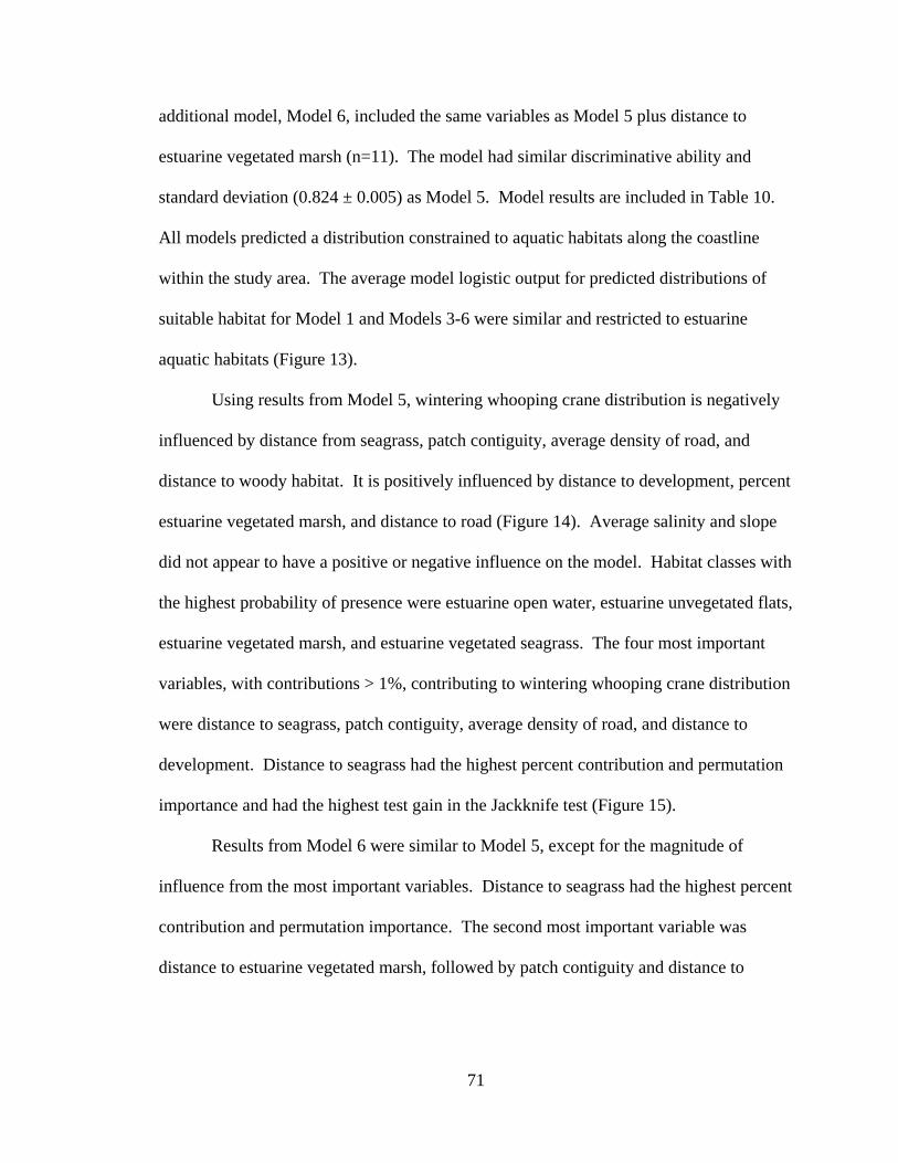
71

additional model, Model 6, included the same variables as Model 5 plus distance to

estuarine vegetated marsh (n=11). The model had similar discriminative ability and

standard deviation (0.824 ± 0.005) as Model 5. Model results are included in Table 10.

All models predicted a distribution constrained to aquatic habitats along the coastline

within the study area. The average model logistic output for predicted distributions of

suitable habitat for Model 1 and Models 3-6 were similar and restricted to estuarine

aquatic habitats (Figure 13).

Using results from Model 5, wintering whooping crane distribution is negatively

influenced by distance from seagrass, patch contiguity, average density of road, and

distance to woody habitat. It is positively influenced by distance to development, percent

estuarine vegetated marsh, and distance to road (Figure 14). Average salinity and slope

did not appear to have a positive or negative influence on the model. Habitat classes with

the highest probability of presence were estuarine open water, estuarine unvegetated flats,

estuarine vegetated marsh, and estuarine vegetated seagrass. The four most important

variables, with contributions > 1%, contributing to wintering whooping crane distribution

were distance to seagrass, patch contiguity, average density of road, and distance to

development. Distance to seagrass had the highest percent contribution and permutation

importance and had the highest test gain in the Jackknife test (Figure 15).

Results from Model 6 were similar to Model 5, except for the magnitude of

influence from the most important variables. Distance to seagrass had the highest percent

contribution and permutation importance. The second most important variable was

distance to estuarine vegetated marsh, followed by patch contiguity and distance to

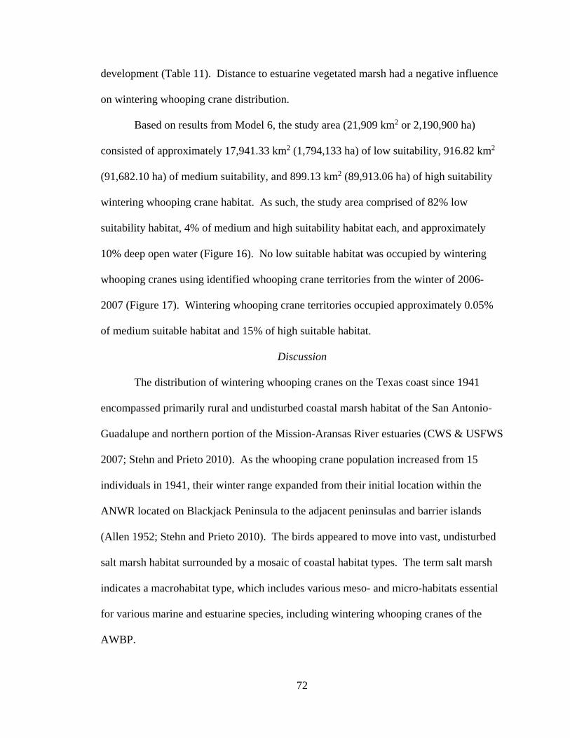
72

development (Table 11). Distance to estuarine vegetated marsh had a negative influence

on wintering whooping crane distribution.

Based on results from Model 6, the study area (21,909 km2 or 2,190,900 ha)

consisted of approximately 17,941.33 km2 (1,794,133 ha) of low suitability, 916.82 km2

(91,682.10 ha) of medium suitability, and 899.13 km2 (89,913.06 ha) of high suitability

wintering whooping crane habitat. As such, the study area comprised of 82% low

suitability habitat, 4% of medium and high suitability habitat each, and approximately

10% deep open water (Figure 16). No low suitable habitat was occupied by wintering

whooping cranes using identified whooping crane territories from the winter of 2006-

2007 (Figure 17). Wintering whooping crane territories occupied approximately 0.05%

of medium suitable habitat and 15% of high suitable habitat.

Discussion

The distribution of wintering whooping cranes on the Texas coast since 1941

encompassed primarily rural and undisturbed coastal marsh habitat of the San Antonio-

Guadalupe and northern portion of the Mission-Aransas River estuaries (CWS & USFWS

2007; Stehn and Prieto 2010). As the whooping crane population increased from 15

individuals in 1941, their winter range expanded from their initial location within the

ANWR located on Blackjack Peninsula to the adjacent peninsulas and barrier islands

(Allen 1952; Stehn and Prieto 2010). The birds appeared to move into vast, undisturbed

salt marsh habitat surrounded by a mosaic of coastal habitat types. The term salt marsh

indicates a macrohabitat type, which includes various meso- and micro-habitats essential

for various marine and estuarine species, including wintering whooping cranes of the

AWBP.

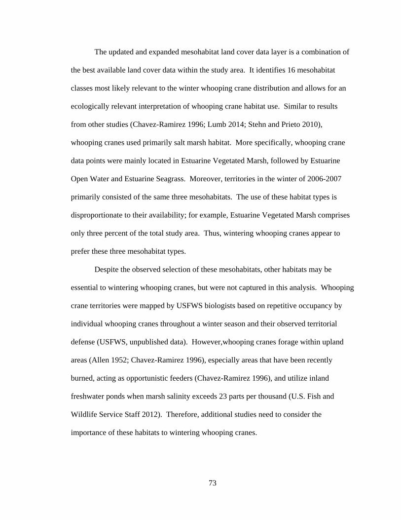
73

The updated and expanded mesohabitat land cover data layer is a combination of

the best available land cover data within the study area. It identifies 16 mesohabitat

classes most likely relevant to the winter whooping crane distribution and allows for an

ecologically relevant interpretation of whooping crane habitat use. Similar to results

from other studies (Chavez-Ramirez 1996; Lumb 2014; Stehn and Prieto 2010),

whooping cranes used primarily salt marsh habitat. More specifically, whooping crane

data points were mainly located in Estuarine Vegetated Marsh, followed by Estuarine

Open Water and Estuarine Seagrass. Moreover, territories in the winter of 2006-2007

primarily consisted of the same three mesohabitats. The use of these habitat types is

disproportionate to their availability; for example, Estuarine Vegetated Marsh comprises

only three percent of the total study area. Thus, wintering whooping cranes appear to

prefer these three mesohabitat types.

Despite the observed selection of these mesohabitats, other habitats may be

essential to wintering whooping cranes, but were not captured in this analysis. Whooping

crane territories were mapped by USFWS biologists based on repetitive occupancy by

individual whooping cranes throughout a winter season and their observed territorial

defense (USFWS, unpublished data). However,whooping cranes forage within upland

areas (Allen 1952; Chavez-Ramirez 1996), especially areas that have been recently

burned, acting as opportunistic feeders (Chavez-Ramirez 1996), and utilize inland

freshwater ponds when marsh salinity exceeds 23 parts per thousand (U.S. Fish and

Wildlife Service Staff 2012). Therefore, additional studies need to consider the

importance of these habitats to wintering whooping cranes.

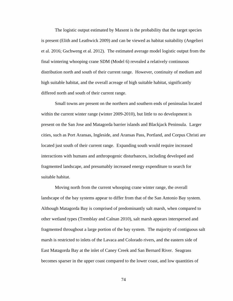
74

The logistic output estimated by Maxent is the probability that the target species

is present (Elith and Leathwick 2009) and can be viewed as habitat suitability (Angelieri

et al. 2016; Gschweng et al. 2012). The estimated average model logistic output from the

final wintering whooping crane SDM (Model 6) revealed a relatively continuous

distribution north and south of their current range. However, continuity of medium and

high suitable habitat, and the overall acreage of high suitable habitat, significantly

differed north and south of their current range.

Small towns are present on the northern and southern ends of peninsulas located

within the current winter range (winter 2009-2010), but little to no development is

present on the San Jose and Matagorda barrier islands and Blackjack Peninsula. Larger

cities, such as Port Aransas, Ingleside, and Aransas Pass, Portland, and Corpus Christi are

located just south of their current range. Expanding south would require increased

interactions with humans and anthropogenic disturbances, including developed and

fragmented landscape, and presumably increased energy expenditure to search for

suitable habitat.

Moving north from the current whooping crane winter range, the overall

landscape of the bay systems appear to differ from that of the San Antonio Bay system.

Although Matagorda Bay is comprised of predominantly salt marsh, when compared to

other wetland types (Tremblay and Calnan 2010), salt marsh appears interspersed and

fragmented throughout a large portion of the bay system. The majority of contiguous salt

marsh is restricted to inlets of the Lavaca and Colorado rivers, and the eastern side of

East Matagorda Bay at the inlet of Caney Creek and San Bernard River. Seagrass

becomes sparser in the upper coast compared to the lower coast, and low quantities of

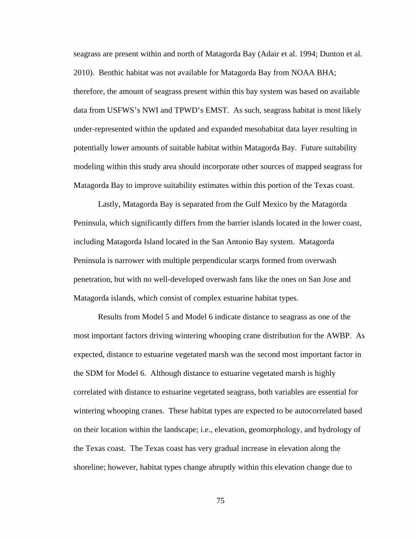
75

seagrass are present within and north of Matagorda Bay (Adair et al. 1994; Dunton et al.

2010). Benthic habitat was not available for Matagorda Bay from NOAA BHA;

therefore, the amount of seagrass present within this bay system was based on available

data from USFWS’s NWI and TPWD’s EMST. As such, seagrass habitat is most likely

under-represented within the updated and expanded mesohabitat data layer resulting in

potentially lower amounts of suitable habitat within Matagorda Bay. Future suitability

modeling within this study area should incorporate other sources of mapped seagrass for

Matagorda Bay to improve suitability estimates within this portion of the Texas coast.

Lastly, Matagorda Bay is separated from the Gulf Mexico by the Matagorda

Peninsula, which significantly differs from the barrier islands located in the lower coast,

including Matagorda Island located in the San Antonio Bay system. Matagorda

Peninsula is narrower with multiple perpendicular scarps formed from overwash

penetration, but with no well-developed overwash fans like the ones on San Jose and

Matagorda islands, which consist of complex estuarine habitat types.

Results from Model 5 and Model 6 indicate distance to seagrass as one of the

most important factors driving wintering whooping crane distribution for the AWBP. As

expected, distance to estuarine vegetated marsh was the second most important factor in

the SDM for Model 6. Although distance to estuarine vegetated marsh is highly

correlated with distance to estuarine vegetated seagrass, both variables are essential for

wintering whooping cranes. These habitat types are expected to be autocorrelated based

on their location within the landscape; i.e., elevation, geomorphology, and hydrology of

the Texas coast. The Texas coast has very gradual increase in elevation along the

shoreline; however, habitat types change abruptly within this elevation change due to

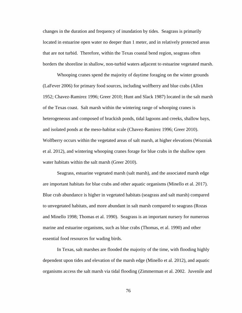
76

changes in the duration and frequency of inundation by tides. Seagrass is primarily

located in estuarine open water no deeper than 1 meter, and in relatively protected areas

that are not turbid. Therefore, within the Texas coastal bend region, seagrass often

borders the shoreline in shallow, non-turbid waters adjacent to estuarine vegetated marsh.

Whooping cranes spend the majority of daytime foraging on the winter grounds

(LaFever 2006) for primary food sources, including wolfberry and blue crabs (Allen

1952; Chavez-Ramirez 1996; Greer 2010; Hunt and Slack 1987) located in the salt marsh

of the Texas coast. Salt marsh within the wintering range of whooping cranes is

heterogeneous and composed of brackish ponds, tidal lagoons and creeks, shallow bays,

and isolated ponds at the meso-habitat scale (Chavez-Ramirez 1996; Greer 2010).

Wolfberry occurs within the vegetated areas of salt marsh, at higher elevations (Wozniak

et al. 2012), and wintering whooping cranes forage for blue crabs in the shallow open

water habitats within the salt marsh (Greer 2010).

Seagrass, estuarine vegetated marsh (salt marsh), and the associated marsh edge

are important habitats for blue crabs and other aquatic organisms (Minello et al. 2017).

Blue crab abundance is higher in vegetated habitats (seagrass and salt marsh) compared

to unvegetated habitats, and more abundant in salt marsh compared to seagrass (Rozas

and Minello 1998; Thomas et al. 1990). Seagrass is an important nursery for numerous

marine and estuarine organisms, such as blue crabs (Thomas, et al. 1990) and other

essential food resources for wading birds.

In Texas, salt marshes are flooded the majority of the time, with flooding highly

dependent upon tides and elevation of the marsh edge (Minello et al. 2012), and aquatic

organisms access the salt marsh via tidal flooding (Zimmerman et al. 2002. Juvenile and

77

adult blue crabs have been recorded to migrate out of nearby nurseries into salt marsh in

relation to an increase in size (Greer 2010), becoming available to wintering whooping

cranes. Moreover, high densities of juvenile blue crabs and other aquatic organisms have

been found within in the first few meters of vegetated salt marsh adjacent to open water

(LaFever 2006; Minello et al. 2008). Some food sources are available in upland habitats

and shallow open water (<50-80 cm) of the bay; however, wintering whooping cranes are

documented to spend significantly less time in these habitats and appear to depend on

these habitats only when other food sources are scarce (Chavez-Ramirez 1996).

Wintering whooping cranes consistently consume wolfberry fruits, blue crabs, clams,

snails, and insects. Whooping cranes are opportunistic feeders; however, these foods are

selected out of multiple available food resources, suggesting they are most optimal

compared to other available foods (Greer 2010).

The flux of tides in coastal areas allow for spatial and temporal habitat

heterogeneity (Drew et al. 2013) and, therefore, influence salt marsh and seagrass

habitats that provide food resources for wintering whooping cranes. Both habitat types

are key drivers in the distribution of whooping cranes along the Texas coast, however,

tidal cycles are also integral to their distribution within the winter season; i.e., monthly

distribution within a winter season. For example, when wolfberry fruit and blue crabs

were both at peak abundance, whooping cranes consumed large quantities of wolfberry

fruit compared to blue crab between November and December. Therefore, whooping

cranes were predominantly located in the mid- to high-marsh (Greer 2010). Once the

fruit abundance declined, whooping cranes gradually switched to blue crab as their main

diet and moved into the lower salt marsh. Presumably, high tides hindered access to blue

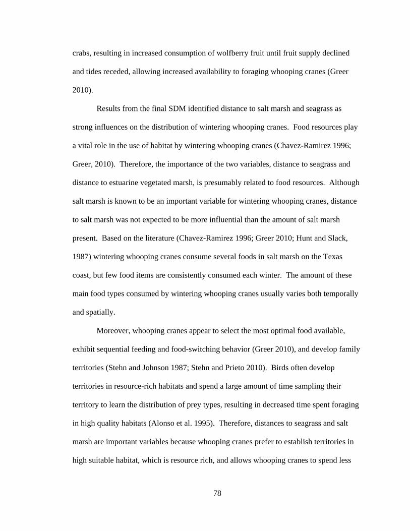
78

crabs, resulting in increased consumption of wolfberry fruit until fruit supply declined

and tides receded, allowing increased availability to foraging whooping cranes (Greer

2010).

Results from the final SDM identified distance to salt marsh and seagrass as

strong influences on the distribution of wintering whooping cranes. Food resources play

a vital role in the use of habitat by wintering whooping cranes (Chavez-Ramirez 1996;

Greer, 2010). Therefore, the importance of the two variables, distance to seagrass and

distance to estuarine vegetated marsh, is presumably related to food resources. Although

salt marsh is known to be an important variable for wintering whooping cranes, distance

to salt marsh was not expected to be more influential than the amount of salt marsh

present. Based on the literature (Chavez-Ramirez 1996; Greer 2010; Hunt and Slack,

1987) wintering whooping cranes consume several foods in salt marsh on the Texas

coast, but few food items are consistently consumed each winter. The amount of these

main food types consumed by wintering whooping cranes usually varies both temporally

and spatially.

Moreover, whooping cranes appear to select the most optimal food available,

exhibit sequential feeding and food-switching behavior (Greer 2010), and develop family

territories (Stehn and Johnson 1987; Stehn and Prieto 2010). Birds often develop

territories in resource-rich habitats and spend a large amount of time sampling their

territory to learn the distribution of prey types, resulting in decreased time spent foraging

in high quality habitats (Alonso et al. 1995). Therefore, distances to seagrass and salt

marsh are important variables because whooping cranes prefer to establish territories in

high suitable habitat, which is resource rich, and allows whooping cranes to spend less

79

time in search of food without success. These results the amount of estuarine marsh and

seagrass habitats is not as important as the accessibility to and availability of important

food resources. This conclusion is further supported by the historical distribution of

whooping cranes within more freshwater habitats prior to increased agriculture and

hunting pressure (Allen 1952).

The negative relationship observed between patch contiguity and habitat

suitability reflects the importance of multiple mesohabitats to the structure of wintering

whooping crane territories. Patch contiguity was calculated within a 2.98-km radius to

coincide with the average territory size documented by Stehn and Prieto (2010). Winter

territories in the winter of 2006-2007 encompassed 11 of the 16 mesohabitat classes,

which translates to low patch contiguity of mesohabitats within a territory. Contiguity of

mesohabitats may have a different effect on the distribution of wintering whooping

cranes if it was calculated at the landscape scale instead of patch scale. For example, the

distribution of whooping cranes can be expected to occur within unoccupied, undisturbed

habitat comprised of contiguous estuarine vegetated marsh, estuarine vegetated seagrass,

and estuarine open water.

The final SDM resulted in a suitability range between 0 and 64 %. Suitability did

not reach 100% due to the amount of variability inherent in the point data. Whooping

crane point data used in this study comprised subadult, paired, and family whooping

crane point data. Based on the literature, subadults do not establish territories and

subsequently use different habitat types than territorial pairs and families. An additional

SDM was developed similar to the final SDM, but with only subadult whooping crane

data points for winters between 2004-2005 and 2009-2010. The suitability index

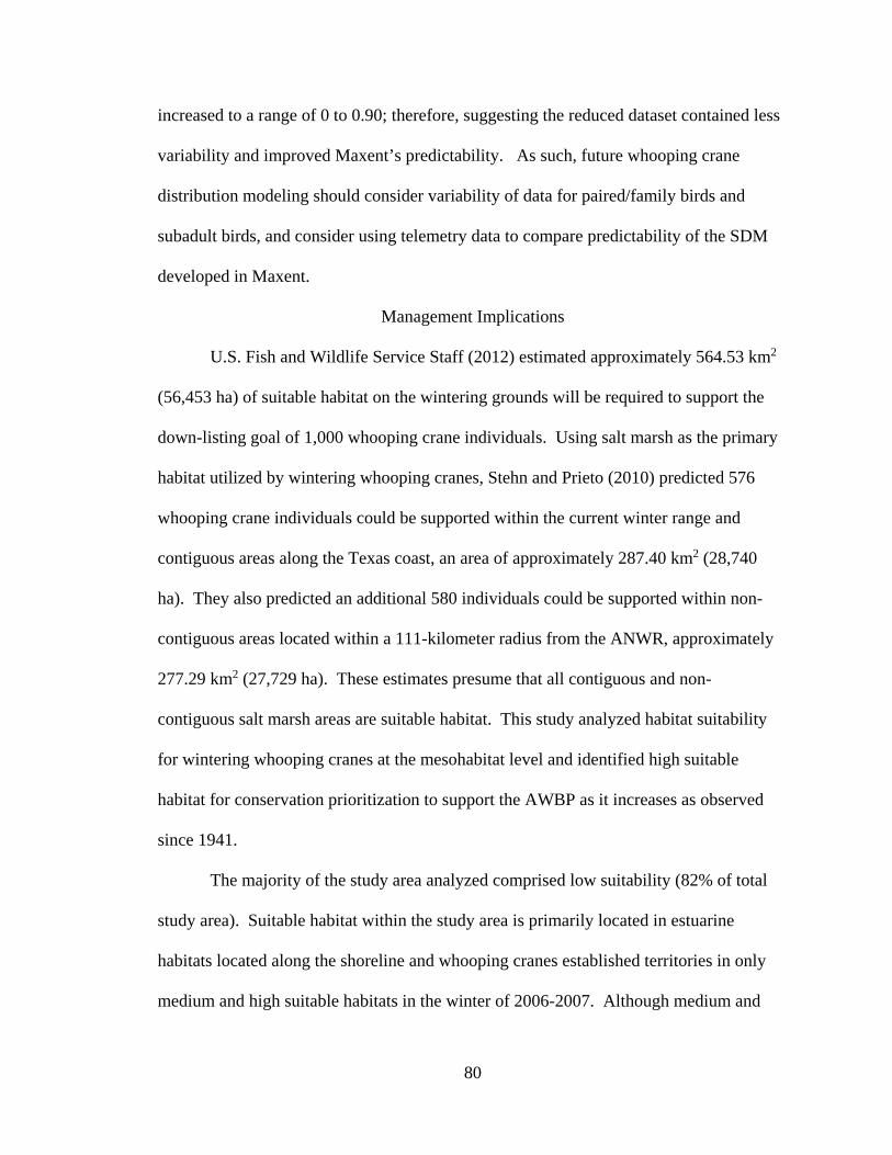
80

increased to a range of 0 to 0.90; therefore, suggesting the reduced dataset contained less

variability and improved Maxent’s predictability. As such, future whooping crane

distribution modeling should consider variability of data for paired/family birds and

subadult birds, and consider using telemetry data to compare predictability of the SDM

developed in Maxent.

Management Implications

U.S. Fish and Wildlife Service Staff (2012) estimated approximately 564.53 km2

(56,453 ha) of suitable habitat on the wintering grounds will be required to support the

down-listing goal of 1,000 whooping crane individuals. Using salt marsh as the primary

habitat utilized by wintering whooping cranes, Stehn and Prieto (2010) predicted 576

whooping crane individuals could be supported within the current winter range and

contiguous areas along the Texas coast, an area of approximately 287.40 km2 (28,740

ha). They also predicted an additional 580 individuals could be supported within non-

contiguous areas located within a 111-kilometer radius from the ANWR, approximately

277.29 km2 (27,729 ha). These estimates presume that all contiguous and non-

contiguous salt marsh areas are suitable habitat. This study analyzed habitat suitability

for wintering whooping cranes at the mesohabitat level and identified high suitable

habitat for conservation prioritization to support the AWBP as it increases as observed

since 1941.

The majority of the study area analyzed comprised low suitability (82% of total

study area). Suitable habitat within the study area is primarily located in estuarine

habitats located along the shoreline and whooping cranes established territories in only

medium and high suitable habitats in the winter of 2006-2007. Although medium and

81

high suitable habitat consists of only eight percent of the study area, the total amount

(181,595.16 ha) is greater than the 56,453 ha that is the proposed amount necessary to

support 1,000 individual whooping cranes (Stehn and Prieto 2010; U.S. Fish and Wildlife

Service Staff, 2012). Based on winter territories from the winter of 2006-2007, less than

20% of the available medium and high suitable habitat is occupied by territorial

whooping cranes. This estimate has presumably increased as the population has

increased since 2006 and does not consider non-territorial habitat use.

Although the amount of suitable habitat within the study area seems more than

enough to support 1,000 individual birds, additional factors may influence the overall

suitability of unoccupied areas and need to be considered when deciding on conservation

measures. Social and behavioral characteristics have shown to be key elements in the

spatial distribution of wintering birds (Coates et al. 2014; Gshweng et al. 2012). Thus,

the identified key variables from the developed SDM are not the only major factors

influencing the distribution of wintering whooping cranes. For example, the overall

dispersal of whooping cranes on the Texas coast appears to move in a northward

progression despite the presence of suitable habitat south of ANWR based on results

from this study.

Whooping cranes seem to disperse in an orderly progression outwards from

ANWR, which reflects the tendency of males to establish territories adjacent to their

family where they spent their first winter (Stehn and Johnson 1987). However, the range

has expanded beyond ANWR by the dispersal of individual birds into new, unoccupied

salt marsh, presumably due to carrying capacity on Blackjack Peninsula (Stehn and Prieto

2010). It is still unclear as to why northward expansion is predominant. Presumably,

82

anthropogenic pressure further south and the presence of black mangrove (Avicennia

germinans) hinder expansion further south (Stehn and Prieto 2010). However, whooping

cranes may also be less familiar with the southern landscape identified as suitable habitat

from this study due to lack of wandering. Subadult whooping cranes do not establish

territories and spend more time in areas outside occupied territories (Bishop and

Blankenship 1981). Therefore, the expansion of the whooping crane population may be

significantly dependent on the experiences and knowledge gained by subadult whooping

cranes.

Whooping cranes have been observed to establish territories on the winter

grounds within unoccupied salt marsh adjacent to occupied territories (Stehn and Prieto

2010), resulting in a gradual expansion along the Texas coast, with little to no gaps of

unoccupied marsh between the territories. Therefore, due to the density of cities, roads,

and other anthropogenic features south of the current whooping crane range, and their

observed propensity to establish territories near the parental territory of the male partner

(Stehn and Johnson 1987; Stehn and Prieto 2010), wintering whooping cranes will most

likely expand northward along the Texas coast into undisturbed and unoccupied salt

marsh. Therefore, conservation strategies should focus on the protection and

enhancement of winter whooping crane habitat north of their current winter range.

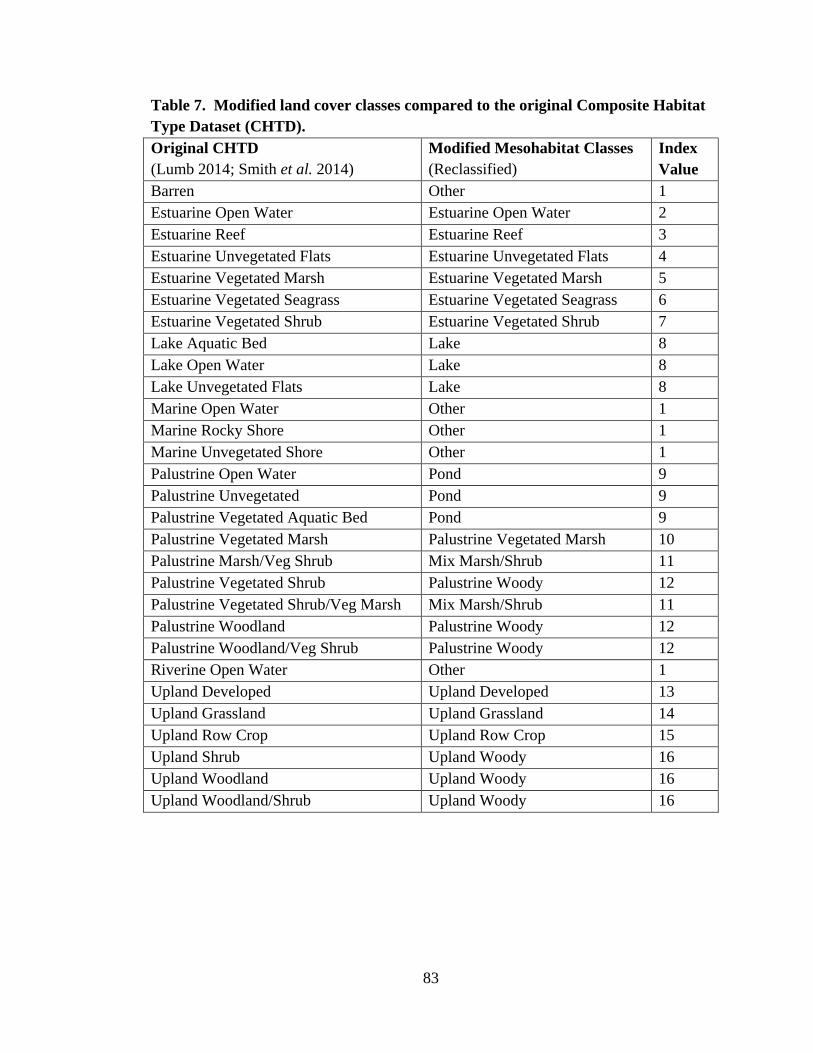
83

Table 7. Modified land cover classes compared to the original Composite Habitat Type Dataset (CHTD). Original CHTD (Lumb 2014; Smith et al. 2014)

Modified Mesohabitat Classes (Reclassified)

Index Value

Barren Other 1 Estuarine Open Water Estuarine Open Water 2 Estuarine Reef Estuarine Reef 3 Estuarine Unvegetated Flats Estuarine Unvegetated Flats 4 Estuarine Vegetated Marsh Estuarine Vegetated Marsh 5 Estuarine Vegetated Seagrass Estuarine Vegetated Seagrass 6 Estuarine Vegetated Shrub Estuarine Vegetated Shrub 7 Lake Aquatic Bed Lake 8 Lake Open Water Lake 8 Lake Unvegetated Flats Lake 8 Marine Open Water Other 1 Marine Rocky Shore Other 1 Marine Unvegetated Shore Other 1 Palustrine Open Water Pond 9 Palustrine Unvegetated Pond 9 Palustrine Vegetated Aquatic Bed Pond 9 Palustrine Vegetated Marsh Palustrine Vegetated Marsh 10 Palustrine Marsh/Veg Shrub Mix Marsh/Shrub 11 Palustrine Vegetated Shrub Palustrine Woody 12 Palustrine Vegetated Shrub/Veg Marsh Mix Marsh/Shrub 11 Palustrine Woodland Palustrine Woody 12 Palustrine Woodland/Veg Shrub Palustrine Woody 12 Riverine Open Water Other 1 Upland Developed Upland Developed 13 Upland Grassland Upland Grassland 14 Upland Row Crop Upland Row Crop 15 Upland Shrub Upland Woody 16 Upland Woodland Upland Woody 16 Upland Woodland/Shrub Upland Woody 16

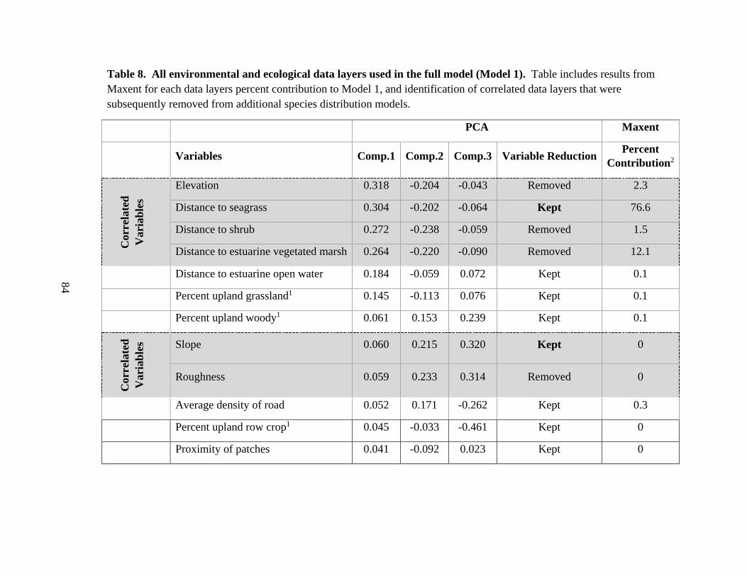
84

Table 8. All environmental and ecological data layers used in the full model (Model 1). Table includes results from Maxent for each data layers percent contribution to Model 1, and identification of correlated data layers that were subsequently removed from additional species distribution models.

PCA Maxent

Variables Comp.1 Comp.2 Comp.3 Variable Reduction Percent Contribution2

Cor

rela

ted

Var

iabl

es

Elevation 0.318 -0.204 -0.043 Removed 2.3

Distance to seagrass 0.304 -0.202 -0.064 Kept 76.6

Distance to shrub 0.272 -0.238 -0.059 Removed 1.5

Distance to estuarine vegetated marsh 0.264 -0.220 -0.090 Removed 12.1

Distance to estuarine open water 0.184 -0.059 0.072 Kept 0.1

Percent upland grassland1 0.145 -0.113 0.076 Kept 0.1

Percent upland woody1 0.061 0.153 0.239 Kept 0.1

Cor

rela

ted

Var

iabl

es Slope 0.060 0.215 0.320 Kept 0

Roughness 0.059 0.233 0.314 Removed 0

Average density of road 0.052 0.171 -0.262 Kept 0.3

Percent upland row crop1 0.045 -0.033 -0.461 Kept 0

Proximity of patches 0.041 -0.092 0.023 Kept 0

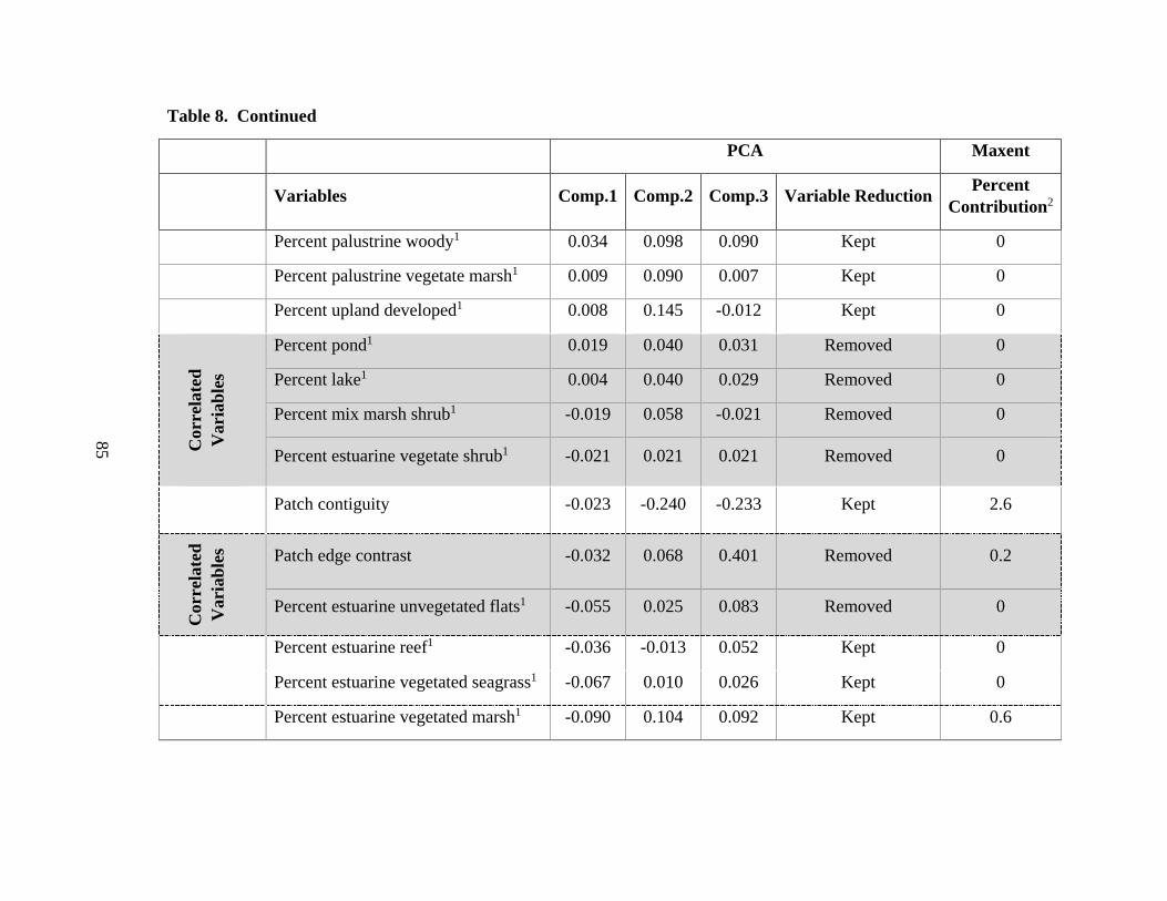
85

Table 8. Continued

PCA Maxent

Variables Comp.1 Comp.2 Comp.3 Variable Reduction Percent Contribution2

Percent palustrine woody1 0.034 0.098 0.090 Kept 0

Percent palustrine vegetate marsh1 0.009 0.090 0.007 Kept 0

Percent upland developed1 0.008 0.145 -0.012 Kept 0

Cor

rela

ted

Var

iabl

es

Percent pond1 0.019 0.040 0.031 Removed 0

Percent lake1 0.004 0.040 0.029 Removed 0

Percent mix marsh shrub1 -0.019 0.058 -0.021 Removed 0

Percent estuarine vegetate shrub1 -0.021 0.021 0.021 Removed 0

Patch contiguity -0.023 -0.240 -0.233 Kept 2.6

Cor

rela

ted

Var

iabl

es

Patch edge contrast -0.032 0.068 0.401 Removed 0.2

Percent estuarine unvegetated flats1 -0.055 0.025 0.083 Removed 0

Percent estuarine reef1 -0.036 -0.013 0.052 Kept 0

Percent estuarine vegetated seagrass1 -0.067 0.010 0.026 Kept 0

Percent estuarine vegetated marsh1 -0.090 0.104 0.092 Kept 0.6

86

Table 8. Continued.

PCA Maxent

Variables Comp.1 Comp.2 Comp.3 Variable Reduction Percent Contribution2

Distance to development -0.169 -0.287 0.212 Kept 1

Distance to road -0.196 -0.203 0.276 Kept 0.4

Cor

rela

ted

Var

iabl

es

Distance to freshwater -0.225 -0.293 0.024 Removed 0

Distance to woody cover -0.239 -0.310 0.005 Kept 0.4

Patch area -0.242 -0.286 0.006 Removed 0.4

Percent estuarine open water1 -0.265 -0.255 0.054 Removed 0.1

Cor

rela

ted

Var

iabl

es Minimum salinity -0.261 0.165 0.046 Removed 0.2

Average salinity -0.307 0.140 0.054 Kept 0.3

Maximum salinity -0.321 0.124 0.059 Removed 0.4

Mesohabitat classes3 - - - - 0.2

Hydric Soils3 - - - - 0 1 Percent calculated in 3-cell by 3-cell neighborhood 2 Percent contribution calculated by Maxent (West et al. 2015) from the preliminary full model (Model 1) 3 Categorical data not included in PCA

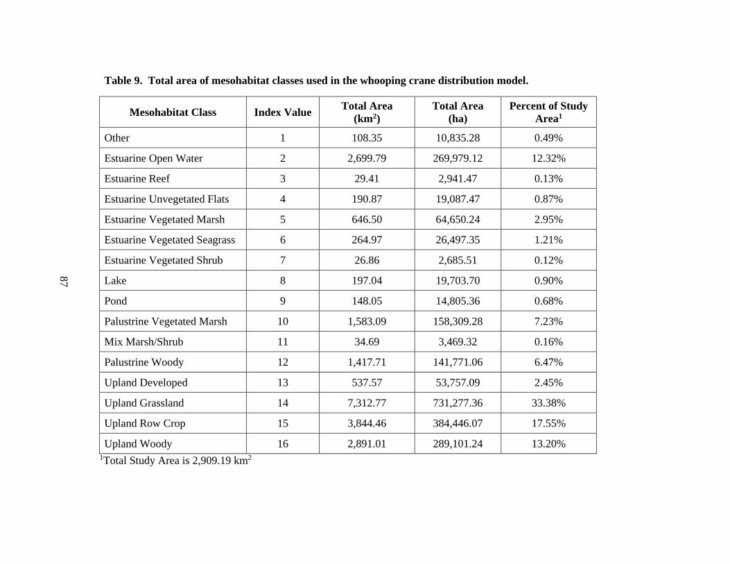
87

Table 9. Total area of mesohabitat classes used in the whooping crane distribution model.

Mesohabitat Class Index Value Total Area (km2)

Total Area (ha)

Percent of Study Area1

Other 1 108.35 10,835.28 0.49%

Estuarine Open Water 2 2,699.79 269,979.12 12.32%

Estuarine Reef 3 29.41 2,941.47 0.13%

Estuarine Unvegetated Flats 4 190.87 19,087.47 0.87%

Estuarine Vegetated Marsh 5 646.50 64,650.24 2.95%

Estuarine Vegetated Seagrass 6 264.97 26,497.35 1.21%

Estuarine Vegetated Shrub 7 26.86 2,685.51 0.12%

Lake 8 197.04 19,703.70 0.90%

Pond 9 148.05 14,805.36 0.68%

Palustrine Vegetated Marsh 10 1,583.09 158,309.28 7.23%

Mix Marsh/Shrub 11 34.69 3,469.32 0.16%

Palustrine Woody 12 1,417.71 141,771.06 6.47%

Upland Developed 13 537.57 53,757.09 2.45%

Upland Grassland 14 7,312.77 731,277.36 33.38%

Upland Row Crop 15 3,844.46 384,446.07 17.55%

Upland Woody 16 2,891.01 289,101.24 13.20% 1Total Study Area is 2,909.19 km2

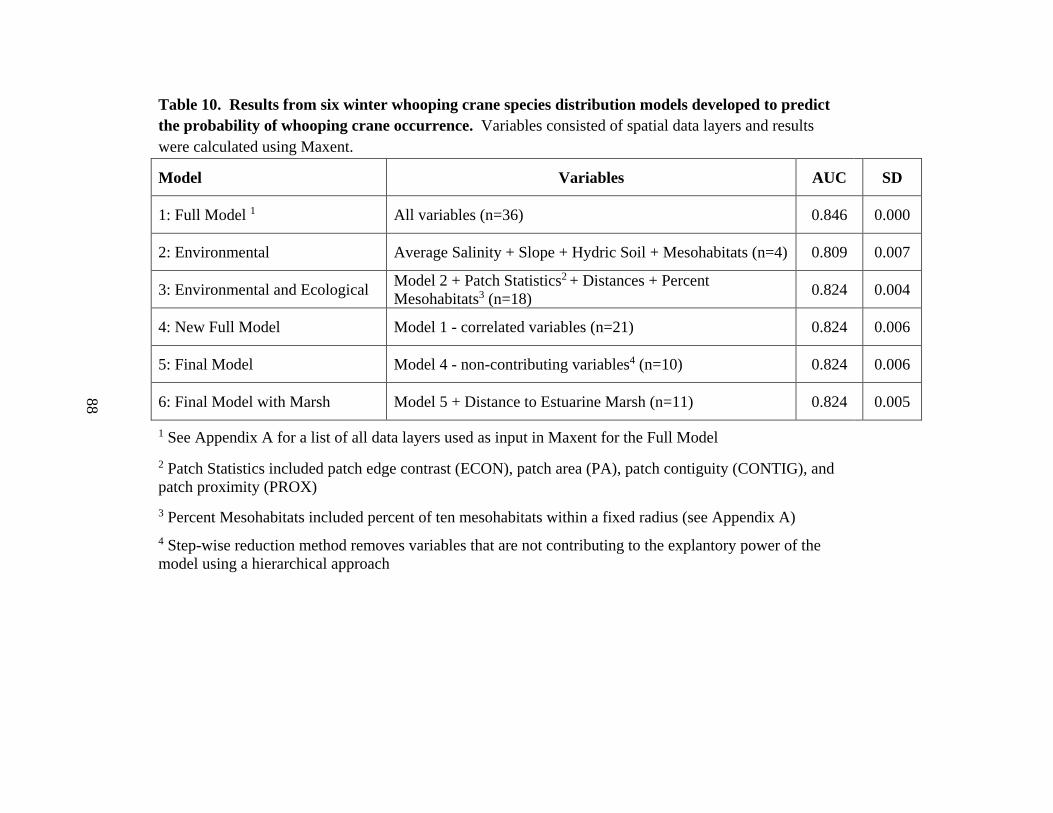
88

Table 10. Results from six winter whooping crane species distribution models developed to predict the probability of whooping crane occurrence. Variables consisted of spatial data layers and results were calculated using Maxent.

Model Variables AUC SD

1: Full Model 1 All variables (n=36) 0.846 0.000

2: Environmental Average Salinity + Slope + Hydric Soil + Mesohabitats (n=4) 0.809 0.007

3: Environmental and Ecological Model 2 + Patch Statistics2 + Distances + Percent Mesohabitats3 (n=18) 0.824 0.004

4: New Full Model Model 1 - correlated variables (n=21) 0.824 0.006

5: Final Model Model 4 - non-contributing variables4 (n=10) 0.824 0.006

6: Final Model with Marsh Model 5 + Distance to Estuarine Marsh (n=11) 0.824 0.005

1 See Appendix A for a list of all data layers used as input in Maxent for the Full Model 2 Patch Statistics included patch edge contrast (ECON), patch area (PA), patch contiguity (CONTIG), and patch proximity (PROX) 3 Percent Mesohabitats included percent of ten mesohabitats within a fixed radius (see Appendix A) 4 Step-wise reduction method removes variables that are not contributing to the explantory power of the model using a hierarchical approach

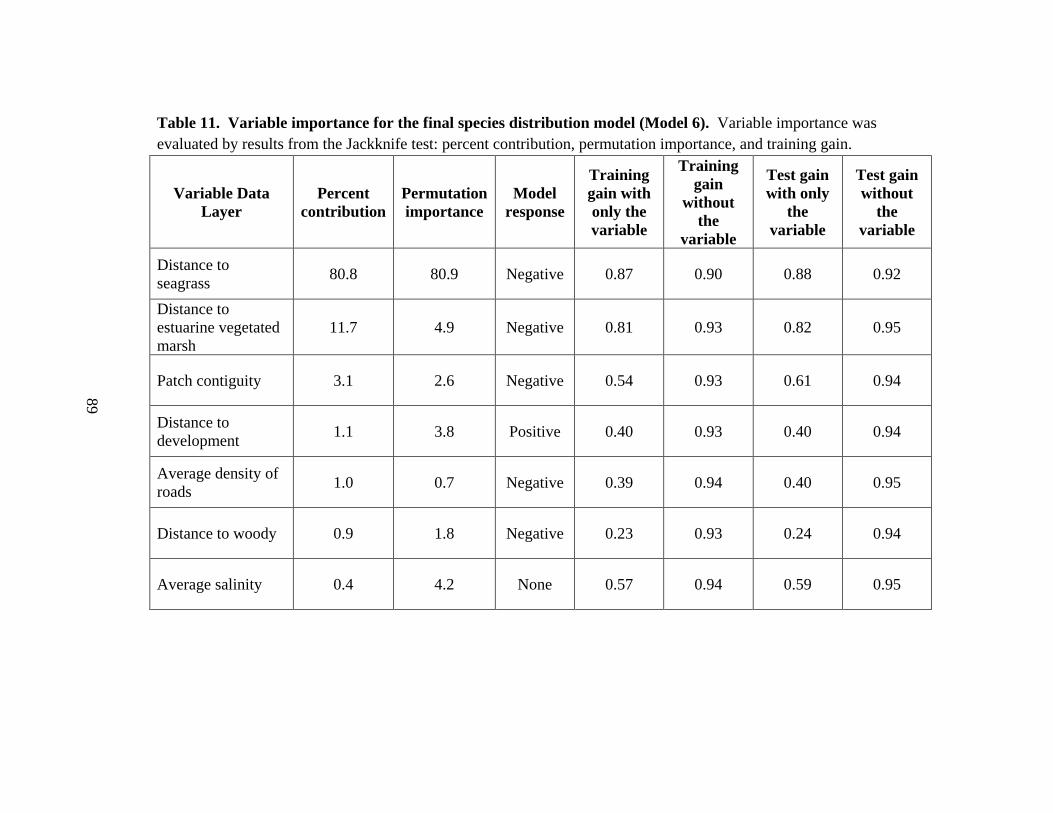
89

Table 11. Variable importance for the final species distribution model (Model 6). Variable importance was evaluated by results from the Jackknife test: percent contribution, permutation importance, and training gain.

Variable Data Layer

Percent contribution

Permutation importance

Model response

Training gain with only the variable

Training gain

without the

variable

Test gain with only

the variable

Test gain without

the variable

Distance to seagrass 80.8 80.9 Negative 0.87 0.90 0.88 0.92

Distance to estuarine vegetated marsh

11.7 4.9 Negative 0.81 0.93 0.82 0.95

Patch contiguity 3.1 2.6 Negative 0.54 0.93 0.61 0.94

Distance to development 1.1 3.8 Positive 0.40 0.93 0.40 0.94

Average density of roads 1.0 0.7 Negative 0.39 0.94 0.40 0.95

Distance to woody 0.9 1.8 Negative 0.23 0.93 0.24 0.94

Average salinity 0.4 4.2 None 0.57 0.94 0.59 0.95

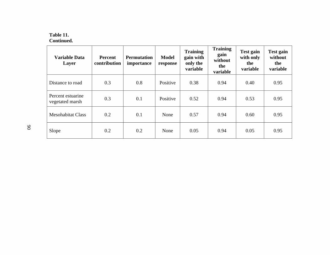
90

Table 11. Continued.

Variable Data Layer

Percent contribution

Permutation importance

Model response

Training gain with only the variable

Training gain

without the

variable

Test gain with only

the variable

Test gain without

the variable

Distance to road 0.3 0.8 Positive 0.38 0.94 0.40 0.95

Percent estuarine vegetated marsh 0.3 0.1 Positive 0.52 0.94 0.53 0.95

Mesohabitat Class 0.2 0.1 None 0.57 0.94 0.60 0.95

Slope 0.2 0.2 None 0.05 0.94 0.05 0.95

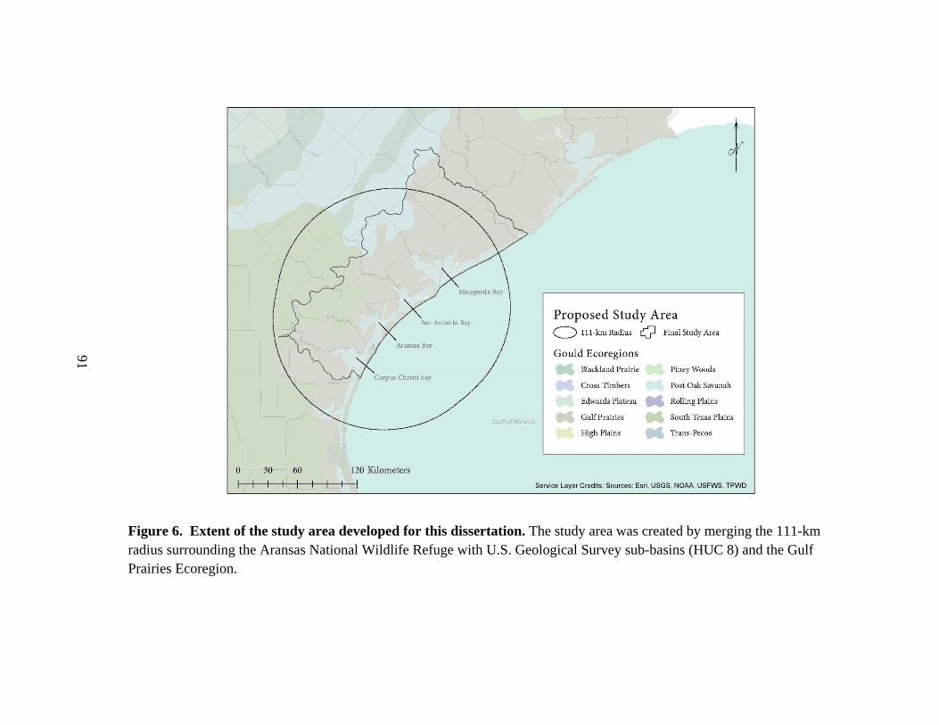
91

Figure 6. Extent of the study area developed for this dissertation. The study area was created by merging the 111-km radius surrounding the Aransas National Wildlife Refuge with U.S. Geological Survey sub-basins (HUC 8) and the Gulf Prairies Ecoregion.

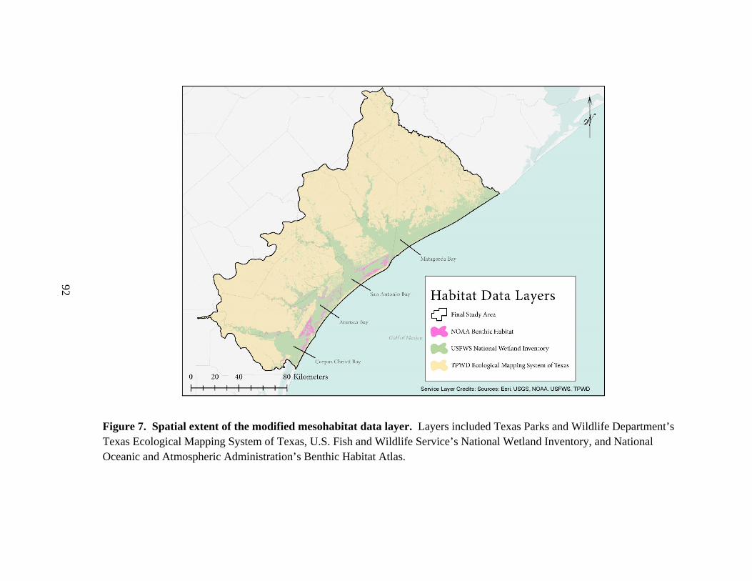
92

Figure 7. Spatial extent of the modified mesohabitat data layer. Layers included Texas Parks and Wildlife Department’s Texas Ecological Mapping System of Texas, U.S. Fish and Wildlife Service’s National Wetland Inventory, and National Oceanic and Atmospheric Administration’s Benthic Habitat Atlas.

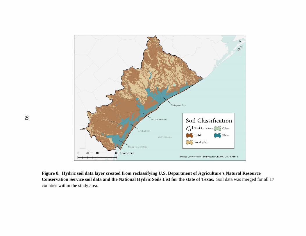
93

Figure 8. Hydric soil data layer created from reclassifying U.S. Department of Agriculture’s Natural Resource Conservation Service soil data and the National Hydric Soils List for the state of Texas. Soil data was merged for all 17 counties within the study area.

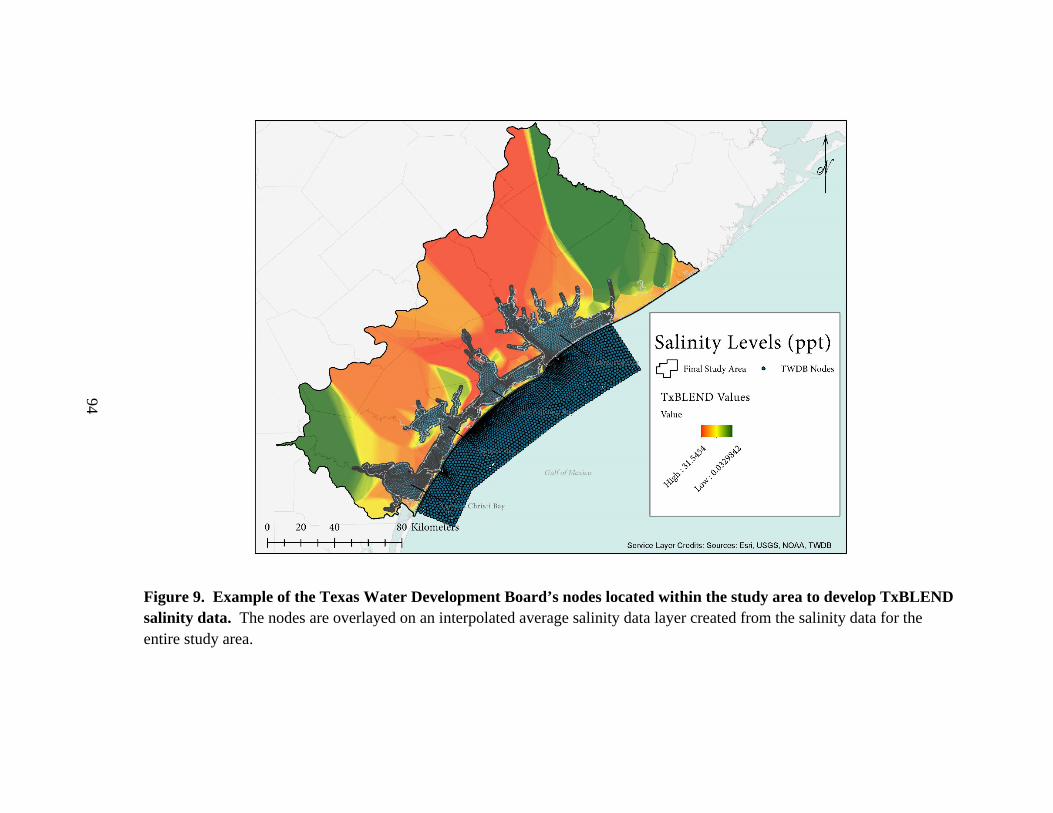
94

Figure 9. Example of the Texas Water Development Board’s nodes located within the study area to develop TxBLEND salinity data. The nodes are overlayed on an interpolated average salinity data layer created from the salinity data for the entire study area.

95

Figure 10. Average salinities within the study area interpolated from Texas Water Development Board’s TXBLEND data for winter months from 2003-2004 to 2009-2010. The inland extent was determined using modeled inundation from National Oceanic and Atmospheric Administration’s SLOSH model for worst-case scenario conditions.

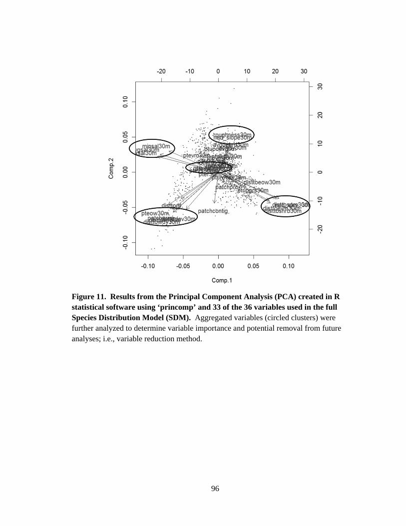
96

Figure 11. Results from the Principal Component Analysis (PCA) created in R statistical software using ‘princomp’ and 33 of the 36 variables used in the full Species Distribution Model (SDM). Aggregated variables (circled clusters) were further analyzed to determine variable importance and potential removal from future analyses; i.e., variable reduction method.

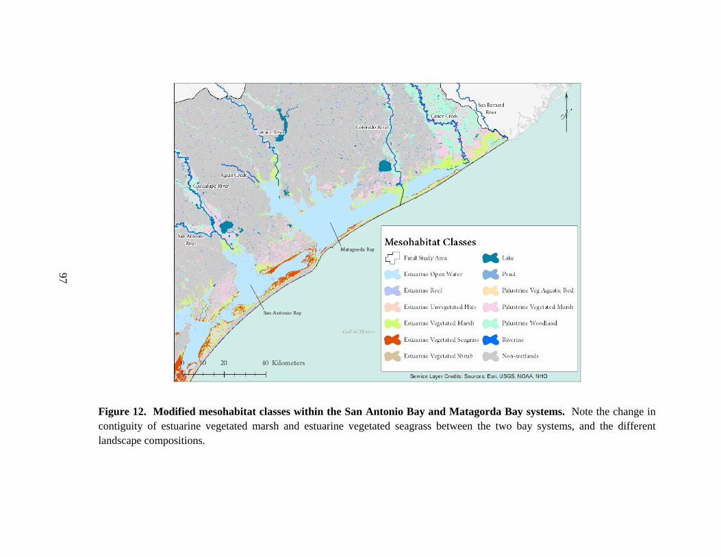
97

Figure 12. Modified mesohabitat classes within the San Antonio Bay and Matagorda Bay systems. Note the change in contiguity of estuarine vegetated marsh and estuarine vegetated seagrass between the two bay systems, and the different landscape compositions.

98

Figure 13. Winter whooping crane suitability values within the study area from four species distribution models comprised of different variables. Note the similarity in suitability values and their distribution within the study area.

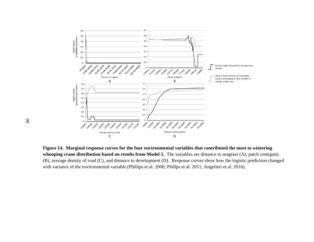
99

Figure 14. Marginal response curves for the four environmental variables that contributed the most to wintering whooping crane distribution based on results from Model 5. The variables are distance to seagrass (A), patch contiguity (B), average density of road (C), and distance to development (D). Response curves show how the logistic prediction changed with variance of the environmental variable (Phillips et al. 2006; Phillps et al. 2011; Angelieri et al. 2016).

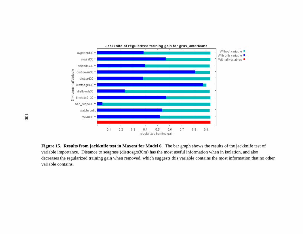
100

Figure 15. Results from jackknife test in Maxent for Model 6. The bar graph shows the results of the jackknife test of variable importance. Distance to seagrass (disttosgrs30m) has the most useful information when in isolation, and also decreases the regularized training gain when removed, which suggests this variable contains the most information that no other variable contains.

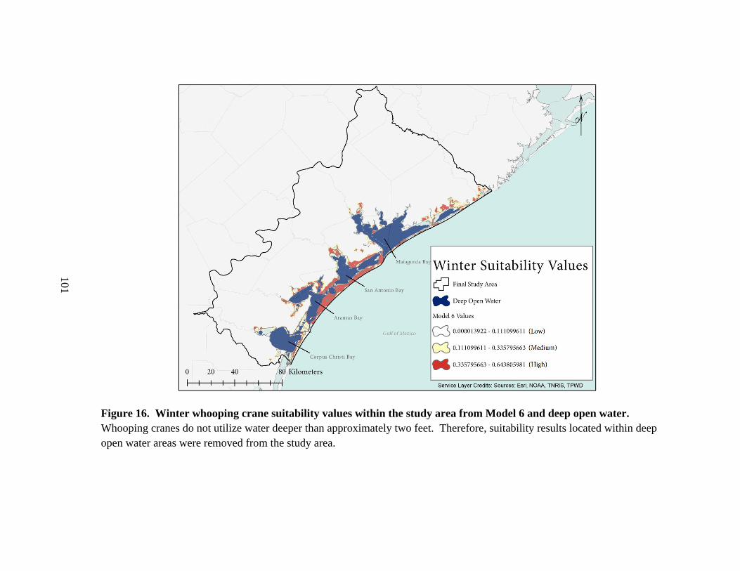
101

Figure 16. Winter whooping crane suitability values within the study area from Model 6 and deep open water. Whooping cranes do not utilize water deeper than approximately two feet. Therefore, suitability results located within deep open water areas were removed from the study area.

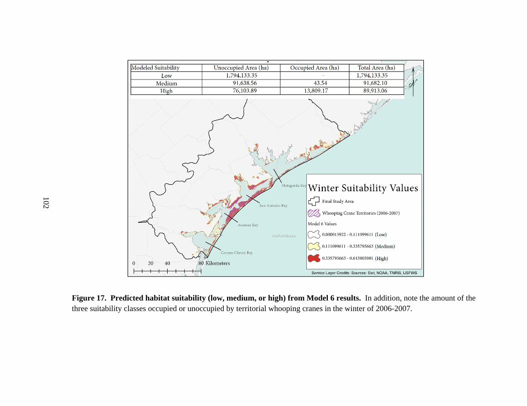
102

Figure 17. Predicted habitat suitability (low, medium, or high) from Model 6 results. In addition, note the amount of the three suitability classes occupied or unoccupied by territorial whooping cranes in the winter of 2006-2007.

103

IV. EVALUATING WINTER RANGE CARRYING CAPACITY IN

ARANSAS-WOOD BUFFALO WHIOOPING CRANE POPULATION

USING MONTE CARLO SIMULATION

In the previous chapter, the final SDM for whooping cranes wintering along the

Texas coast determined approximately 1,816 km2 (181,600 ha) of well-defined suitable

habitat is present within the study area. The study area totaled approximately 21,909 km2

(2,190,900 ha), which includes the current winter range of the AWBP whooping crane

population, as well as surrounding areas perceived as suitable habitat within 111-km

current whooping crane winter range, and a larger extent along the Texas coast than

previously analyzed by Stehn and Prieto (2010), Lumb (2014) or Smith et al. (2014).

Based on the total amount of medium and high suitable habitat from our final SDM and

an average territory size of 1.72 km2 (Stehn and Prieto 2010), 1,056 whooping cranes

could be supported by winter habitat within the study area. Similarly, Stehn and Prieto

(2010) determined that a similar geographical extent comprised of the current winter

range and saltmarsh habitat within a 111-km radius from the ANWR could support a total

of 1,156 whooping cranes.

Both of the estimates outlined above regarding the number of whooping cranes

that could be supported by winter habitat are highly dependent upon underlying

assumptions. Stehn and Prieto (2010) assume that all habitat identified as ‘salt marsh’

within the 111-km radius are suitable for wintering whooping cranes. Moreover, both

Stehn and Prieto (2010) and our SDM include the assumptions that there is a fixed

average territory size throughout the winter range and that individual birds will disperse

into new, non-contiguous areas as long as they are suitable. These estimates do not

104

incorporate dynamic factors that affect species distributions, such as dispersal and spread

patterns, which can provide a link between potential and realized distributions and

improve the estimate of species presence (Merow et al. 2011). By not considering these

factors in SDMs, the overall results may over-estimate the presence whooping cranes in

unreachable locations or underestimate their presence in low-suitability areas with “high

propagule rain” distributions (Franklin 2010; Gallien et al. 2010, Merow et al. 2011).

Abundance of a species is not only based on habitat suitability, but is part of a

relationship between population demography, abundance, and suitability, as shown for

other species (roe deer (Capreolus capreolus); Acedevo et al. 2017). Improving

estimates on species abundance requires large-scale sampling efforts, which is usually

infeasible on large spatial scales. As such, results from SDMs have been used to predict

local species abundance and have been found to predict the upper abundance limit at a

local scale based on the given environmental conditions used to drive the model

(Acedevo et al. 2017). The upper abundance limit can then be used as a proxy for

carrying capacity estimates (Muñoz et al. 2015). Carrying capacity is the limit of a

population size set by food, space, cover, or other resources in a particular environment

(Caughley and Sinclair 1994) and will fluctuate around an equilibrium depending on

resources and environmental variation (Plumb et al. 2009). Estimating carrying capacity

in particular environments is often done by developing spatially-explicit, ecosystem

models that link food production and use, habitat quality and nutrition, nutritional status

of the population, demographic response of the population, and animal energy balances

(Coughenour 2002; Plumb et al. 2009).

105

For the AWBP population, Stehn and Prieto (2010) postulated two carrying

capacity estimates for the winter range. Using the abovementioned average minimum

territory size, they proposed the winter range occupied in the winter of 2009-2010 had a

carrying capacity of 576 birds. However, this estimate did not include space-use by non-

territorial, subadult birds. Therefore, they modified the carrying capacity estimate by

determining each whooping crane individual requires a set amount of area, 0.87 km2 (87

ha) per bird. They then calculated the winter carrying capacity to be 329 whooping

cranes, which is a 42% smaller carrying capacity than estimated using average minimum

territory sizes of 1.72 km2 (i.e., N=576). Based on the difference of the two carrying

capacity estimates, there appears to be a significant uncertainty in carrying capacity

within the winter range of the AWBP whooping crane population.

Territories and Carrying Capacity

Territories and core area sizes are primarily dependent upon the spatial

distribution of resources and intraspecific interactions driving space partitioning (Adams

2001; Valcu and Kempenaers 2010). Two complementary theories focus on territory size

as a result of (1) food abundance; territory size decreases as food becomes more

abundant, and (2) neighbor interactions; territory size increase when neighbor is

removed. Paired and family whooping cranes establish territories within the winter range

that they aggressively defend from other conspecifics (Allen 1950, Stehn and Johnson

1987). Based on winter whooping crane territory mapping conducted by Stehn and Prieto

(2010), the average size of territories established by wintering whooping cranes differed

for each landform that comprises the winter range.

106

In 1950, all AWBP population territories were located within the Blackjack Unit

of the ANWR (N=7). The number of territories within the Blackjack Unit increased to 18

in 1990 and 20 by 2006. Territories within the Blackjack Unit appear to have remained

relatively constant since 1990, averaging approximately 1.01 km2 (101 ha) per

pair/family. Consistent territory sizes from the Blackjack Unit from 1990 to 2010

suggests an overall carrying capacity has been met, and that the landform can only

support 17 to 20 whooping crane territories (Stehn and Prieto 2010). As the population

grew, the first territories established off the Blackjack Unit occurred in non-contiguous

habitat within the Matagorda Unit in 1958, followed by San Jose Island in 1969, Lamar

Peninsula in 1971, and the Welder Flats area on the Seadrift-Port O’Connor Ridge

Peninsula in 1973.

As shown in Table 12, the total area occupied by territories increased from

approximately 22 km2 (2,200 ha) in 1950 to 139 km2 (13,900 ha) in 2006 (Stehn and

Prieto 2010). The average territory size for the total population decreased during this

time from approximately 3.1 km2 (310 ha) in 1950 to 2.1 km2 (210 ha) in 2006.

Similarly, territories located within the Blackjack Unit of ANWR decreased from an

average of approximately 3.1 km2 (310 ha) in 1950 to 1.1 km2 (110 ha) in 1990 and 2006,

when suitable habitat was greater than 90% occupied (Stehn and Prieto 2010). Stehn and

Prieto (2010) predicted the average minimum territory size on ANWR was approaching

1.01 km2 (101 ha), that the average minimum territory size throughout the crane range

was 1.72 km2 (172 ha), and that the current winter range, as of the winter of 2010, could

support 160 territories (Table 13).

107

In addition to patterns observed in territory sizes on different landforms that

comprise the winter grounds, the historical dispersal patterns of the AWBP suggests they

colonize non-contiguous areas of suitable winter habitat close to the occupied range; i.e.,

orderly progression outwards from a territory (Stehn and Prieto 2010). However, it also

appears the location of newly established winter territories is influenced by the preference

of the male bird of the newly paired whooping cranes, establishing a territory next to their

parents and the area where they would have spent their first winter (Stehn and Johnson

1987).

In this chapter, whooping crane distribution was simulated within the winter range

to predict carrying capacities for individual landforms within the study area (current and

predicted winter range). The model simulated the development of territories by paired

and family whooping cranes based on simple rules developed a priori from literature on,

and observation of, the AWB population. Simulations were developed using

randomization and Monte Carlo methods to evaluate carrying capacity of the AWB

whooping crane winter range located within the study area under various space-use

assumptions and predicted suitability values from the previous chapter. Results from the

simulations are then compared with carrying capacity estimates from Stehn and Prieto

(2010) and the estimate of the upper abundance limit of wintering whooping cranes from

our previous SDM.

Using fixed average minimum territory sizes estimated by Stehn and Prieto

(2010), the first simulation uses a randomization approach to allow territories to be

established anywhere within the winter range. The second simulation uses Monte Carlo

methods with varying territory sizes instead of a fixed size to compare carrying capacity

108

results with the previous simulation and the literature. Fluctuations in the number of

territories and their sizes in relation to environmental variations were expected and it was

further hypothesized that:

1. Paired/family and subadult whooping cranes use different habitats depending

on their suitability;

2. Results from our simulations will more accurately predict carrying capacity

for the winter range than previous estimates because it incorporates defined

suitable habitat and space-use strategies; and

3. The Monte Carlo method will more accurately portray the flexibility in

territory sizes developed by wintering whooping cranes, allowing us to better

predict carrying capacity.

Methods

Overall, each simulation started with one bird placed randomly on the landscape,

which comprised of individual raster cells. The bird was assumed to be a paired/family

whooping crane and the simulation allowed them to develop a certain sized territory on

the landscape based on a set of rules. The rules were applied in iterations and included a

review of individual raster cells adjacent to the birds’ location. If the reviewed raster

cells met the rules, those cells were added to a storage vector that represented the birds’

territory. Review of adjacent raster cells continued until the total number of cells equaled

the pre-determined territory size and then another bird was allowed to arrive on the

landscape and begin developing a territory.

All simulations were developed using the study area boundary as the extent of

winter distribution and habitat suitability values from the final SDM (Model 6). The

109

suitability values from the SDM are assumed to be the highest values available along the

Texas coast for wintering whooping cranes due to changes in hydrology that influence

salinity and habitat types within bay systems north and south of the study area. The study

area encompasses 21,909 km2 (2,190,900 ha) within the Gulf Coast Prairies and Marshes

Ecoregion along the Texas coast, includes four out of seven Texas coastal systems:

Nueces-Corpus Christi, Aransas-Copano, San Antonio-Espiritu Santo, and Matagorda-

East Matagorda bays, and is situated within the Texas mid-coast (see Chapter 3, Figure

6). The Texas coast experiences an increasing temperature gradient from north to south

and a decreasing precipitation gradient from east to west. These gradients cause bay

systems within the lower and upper reaches of the Texas coast to differ significantly from

each other and from the bay systems within our study area (Tolan 2006). For example,

the Laguna Madre is a hypersaline system that receives very little freshwater from

precipitation or freshwater inflows from contributing rivers. Suitability values for the

entire study area ranges from 0 to 0.65, and the values were stored in a 30-m raster layer

in ArcMap.

In addition to a suitability index raster, two additional raster layers were created in

ArcMap to store data on occupancy and cell number for each raster cell. Occupancy

could be either 0 or 1 depending if that cell was identified as part of a whooping crane

territory in the simulation. All cells would have an occupancy of 0 prior to initializing

the simulations. To keep track of each cell evaluated in different steps of the simulation,

each raster cell had a unique identifier ranging from 1 to (nrows*ncolumns) of the raster

layer. Cell numbers remained constant throughout the simulations allowing spatial

comparison of territory development in ArcMap. All raster layers were set to the same

110

extent and cell size in ArcMap. All raster layers were uploaded into R 3.5.0 (R

Development Core Team 2018) to perform model simulations. R-scripts are included in

Appendix D. Both simulations incorporate minimum rules to compare estimates on the

total number of territories that can be established on each landform within the study area

to those in the literature. As such, the number of territories that could be established, or

the total number of birds that could create territories, was not predetermined. Each

simulation produces an estimated total number of whooping crane territories that can be

developed based on available suitable habitat within the study area.

Suitability Thresholds and Area

In the previous chapter, suitability values were arbitrarily classified into three

classes: low, medium, and high suitability. These values were based on a natural jenks in

ArcMap, with no consideration to whooping crane biology and medium and high

suitability classes were considered to be suitable winter habitat. To improve our

prediction of what suitability value constitutes suitable habitat for wintering whooping

cranes, suitability classes using winter whooping crane location data points from 1950-

2011 (USFWS) were further evaluated. Location point data was overlaid upon results

from the final SDM (Model 6) using ArcMap to determine if there is a significant

difference in the mean habitat suitability values utilized by paired/family and subadult

whooping cranes. Significance was determined based on t-test results.

The probability of a whooping crane occurring within the range of suitability

values was then determined by calculating probability density functions and 95%

confidence intervals (Som et al. 2015) using the same long-term location data and results

from the SDM (Model 6). Probability of occurrence and cumulative frequency were

111

calculated separately for paired/family (n=1,124) and subadult birds (n=543). Result

from the probability of occurrence for paired/family birds was then used to reclassify the

suitability raster from the previously developed SDM (Model 6) in ArcMap.

Territory Simulations

Randomization and Monte Carlo methods were employed to sample the range of

raster cells that could be included in the establishment of whooping crane territories for

each landform within the study area. The first set of simulations allowed a territory to

become established within suitable areas at random, and expand until reaching a fixed

territory size, determined a priori from the literature (Stehn and Prieto 2010). A total of

ten simulations were run for each landform separately and an average number of

territories was calculated. The next set of simulations used Monte Carlo methods iterated

1,000 times for each landform. This simulation differed from the first simulation because

territory size was not fixed prior to running the simulation. Instead, each iteration used a

random territory size using the Rnorm function in R. The Rnorm function produces a

normal random value using a set mean and standard deviation. As such, the Rnorm

produced various territory sizes based on the mean and standard deviation values derived

from territory sizes mapped in the winter of 2006-2007 (Stehn and Prieto 2010).

Prior to starting the simulation models, each raster cell was assigned an

occupancy value of zero, representing an unoccupied cell, and the three raster layers

(occupancy, suitability, and cell number) were stacked in R to create a raster stack. Each

cell of a raster layer can contain only one attribute or value. A raster stack allows each

cell to contain multiple values depending upon how the raster are stacked, resulting in

faster querying of the data during simulations. For both the fixed and Monte Carlo

112

simulations, unsuitable cells could not be occupied (Rule 1), and territories had to be

established sequentially, with no overlap of territory boundaries among pairs (Rule 2).

Establishment of a territory within the simulation began at a random cell chosen

from the raster stack using a random cell function developed in R. If the random cell was

not available (occupancy value = 0) and suitable (>0.426), the random cell function was

repeated until both conditions were met. The chosen unoccupied and suitable cell

became the focal cell, and the simulation then initiated a neighborhood function

developed in R to evaluate all neighboring cells. The neighborhood function incorporates

the adjacent function in R and a queen’s case that connects adjacent cells in eight

directions within one-cell diagonals from the focal cell (Figure 18). The cell number of

each neighboring cell that is suitable and unoccupied are then stored in a vector (available

cells vector) for future reference, and a expand territory function developed in R is used

to expand the territory outwards from the focal cell. The expand territory function selects

the highest suitable cell within the available cells vector and initiates the adjacent

function using the new cell as the next focal cell and evaluates another eight adjacent

cells (Figure 18). The simulation continues choosing the highest suitable cell stored in

the available cells vector and evaluating adjacent cells until the territory size reaches the

pre-determined limit, which is either a fixed average minimum size or a randomly

selected size for the Monte Carlo method (Rule 3). The territory size is tracked by

storing the total number of available and suitable cells connected from the Adjacent

functions.

If at any time during this expansion process none of the eight adjacent cells are

available and/or suitable, the next focal cell is selected from the previously stored vector

113

of available cells that has not been used as a focal cell. The expand territory function

then resumes to continue developing territories. If all available cells have been used as a

focal cell, and the size threshold has still not been met, the stored values are emptied and

the whooping crane pair is allowed to move to a new random cell and start expanding a

territory in the new location following the aforementioned process (Rule 4).

Throughout the abovementioned simulation process, cells determined to be

suitable and unoccupied during that iteration are listed in a stored vector. Once the

territory size is met, the cells listed in the stored vector are determined to be occupied by

that whooping crane pair, and the occupancy layer in the raster stack is updated to assign

each cell with that pair’s unique ID number; i.e., the first iteration would assign an

occupancy value of 1 to each cell to represent pair 1. The simulation then starts over for

the next pair, starting at a random cell and limiting territory development to only suitable

and unoccupied cells. The simulation continues until no more territories can be

developed on the landform. A simulation was determined complete when a pair moved

more than 20 times in search of available and suitable cells to develop a territory. This

threshold was set based on previous iterations where territories were no longer developed

after a pair moved more than 20 times, and the model appeared to be in an infinite loop of

the same pair continuously moving to new random cells not able to develop a territory.

Evaluation of Habitat Use and Conservation

Using results from one randomly chosen Monte Carlo simulation for each

landform, the number of suitable cells located outside simulated territories were

evaluated to determine the approximate percentage of unused areas per landform, and the

amount of suitable habitat not protected under a national refuge conservation easement or

114

other type of land protection. Suitable habitat not located within a protected area was

calculated by converting the previously reclassified suitability raster to a polygon

shapefile and clipping suitable areas to USGS’s Protected Areas Database of the United

States (PAD-US) version 1.1 (Gergely and McKerrow 2016) in ArcMap.

Results

Results from the t-test comparing the mean habitat suitability used by

paired/family and subadult birds suggests these classes have significantly different space-

use strategies affecting their spatial distribution on the winter grounds (df=19,174,

t=12.10, p< 0.001). Probability density functions allowed the reduction of potential

suitable habitat used by wintering whooping cranes to areas with ≥ 0.30 suitability

(Figure 19). Based on the cumulative frequency of whooping locations and habitat

suitability values, subadult birds occupy areas with suitability as low as 0.331, whereas

paired/family birds are more restrictive in their distribution, and rarely occupy areas with

suitability <0.426 (Table 14). Based on the reclassification of the suitability raster layer

from the final SDM (Model 6) to reflect results from the cumulative frequency results

(Table 14), a total of approximately 483.17 km2 (48,317 ha) of suitable habitat is present

for paired/family birds, and approximately 812.56 km2 (81,256 ha) of additional suitable

habitat is present for subadult birds within the study area (Figure 20).

Territory simulations were initially developed to expand from a focal cell into the

eight surrounding cells by selecting the highest suitable and available cell from the

adjacent function (eight potential cells) instead of selecting the highest suitable cell from

the ‘stored’ available suitable cell vector. This caused the established territory to be

patchy, with multiple unoccupied cells throughout the center (Figure 21). Whooping

115

cranes establish and defend large territories comprised of primarily highly suitable

habitat. As such, not allowing the territory to become established in the direction of the

highest suitable habitat with gaps throughout the territory is unrealistic and ecologically

irrelevant. Therefore, the model approach was modified to allow a pair to occupy the

most suitable habitat as they developed the territory, which better reflects observed

space-use strategies of the AWB population as shown from mapped territories overlaid

upon simulated territories (Figure 22).

Total number of estimated territories for each landform from both the

randomization and Monte Carlo approach are included in Table 15. Visualization of the

estimated territories are included in Figures 23 and 24. As expected, territories simulated

using the randomization approach resulted in relatively similar estimates as Stehn and

Prieto (2010). This simulation estimated more territories could be established on

Blackjack Peninsula than proposed by Stehn and Prieto (2010), and less could be

established on Matagorda Island, Lamar Peninsula, San Jose Island, and Port O’Connor

Ridged Peninsula. Carrying capacity estimated using the Monte Carlo method were

relatively similar for Lamar Peninsula and San Jose Island (see Table 15). Blackjack

Peninsula and Matagorda Island were estimated to support more territories than estimated

by Stehn and Prieto (2010) and the randomization model, and Port O’Connor Ridge

Peninsula and Lamar Peninsula were estimated to be able to support fewer number of

territories in comparison (see Table 15).

As shown in Figure 25, territories established from the simulation using the

Monte Carlo method did not encapsulate all suitable cells within a landform. In total,

approximately 230.0 km2 (23,000 ha) of suitable habitat for paired/family whooping

116

cranes were not included in established territories, which calculates to only 47% of

suitable habitat for paired/family whooping cranes being utilized for the establishment of

territories based on our simulation model with Monte Carlo methods. Based on the PAD-

US version 1.1 (Gergely and McKerrow 2016), approximately 92.1 km2 (9,210 ha) and

186.3 km2 (18,639 ha) of suitable habitat for subadult and paired/family whooping cranes

is located within protected areas, respectively. Therefore, approximately 237.3 km2

(23,730 ha) of suitable subadult and 296.9 km2 (29,690 ha) of suitable paired/family

whooping crane habitat within the study area is not protected (Figure 26).

Discussion

Whooping cranes are wetland-dependent birds that exhibit high site fidelity and

territoriality in their breeding and wintering grounds. Paired and family whooping cranes

occupy habitat with higher suitability values than subadult birds, and they establish

territories of differing sizes that appear to be constrained to a minimum size. Territories

are dependent upon food abundance and intraspecific interactions that can be difficult to

incorporate in SDMs. Intraspecific interactions between paired/family whooping cranes

are well documented in the literature, but food abundance data is lacking. Therefore,

preliminary simulation models were developed that incorporated simple rules to estimate

territory development and carrying capacity from historical whooping crane location data

and habitat suitability estimates. These simulation models incorporated space-use

strategies of territorial whooping cranes in order to better predict carrying capacity of

each landform within the winter range, establish a preliminary model that can mimic the

observed whooping crane distribution off Blackjack Peninsula, and potentially predict

future range expansion.

117

The final SDM in the previous chapter estimated the study area comprised

approximately 1,816 km2 (181,600 ha). Using whooping crane locations from a long-

term dataset (USFWS) and results from the SDM, winter whooping crane habitat

suitability preferences were further evaluated. Based on cumulative density curves

calculated for subadult and pair/family whooping cranes, suitable habitat for

paired/family cranes was restricted to suitability values >0.426 and suitability values

>0.331 for subadults. Restriction of occupancy to these suitability values resulted in a

total of approximately 1,296 km2 (129,600 ha) suitable habitat for wintering whooping

cranes within the study area. Using the more restrictive habitat suitability values from

the cumulative density curves, the study area is comprised of approximately 520 km2

(52,000 ha) less suitable habitat than previously estimated for wintering whooping

cranes.

Carrying capacity results from the simulations using a fixed average minimum

territory size were similar to previously predicted carrying capacities for landforms

within the current whooping crane winter range (Stehn and Prieto 2010). The largest

differences were for Blackjack Peninsula and Lamar Peninsula, which our models

predicted a higher and lower number of territories, respectively. This difference is most

likely attributed to discrepancies between what Stehn and Prieto (2010) determined was

suitable habitat on these peninsulas and the suitability values incorporated from the

calculated estimates derived in the previous chapter.

Future modeling should consider suitable habitat not encapsulated within

territories established by paired/family birds. Territories are smaller areas located within

a home range that represent an area of more intense use (Barg et al. 2005). In these

118

models, the highest suitability values were chosen first and the territory was then

developed around them. However, less suitable cells that are not incorporated in an

established territory are still essential for wintering whooping cranes. These cells are part

of the winter home ranges for both paired/family and subadult whooping cranes and

provide connectivity and dispersal pathways between more suitable habitats, and provide

an essential buffer from human disturbances and effects of climate change over time

(Goetz et al. 2009).

The protection of suitable winter habitat is critical for the AWBP. With the

exception of San Jose Island, which is a relatively pristine barrier island owned and

managed by a private landowner, the majority of territories established by wintering

whooping cranes are located on federally protected lands. These lands are managed and

maintained to support whooping cranes and other wildlife. In total, approximately 72%

of suitable subadult habitat and 62% of suitable paired/family whooping crane habitat

located within the study area is protected. However, the current concern for future

conservation of the AWBP is protecting suitable habitat where birds will inhabit if the

population continues to grow exponentially. Despite having suitable habitat, the southern

portion of the study area is heavily influenced by industry and development, making it

unlikely whooping crane habitat. In contrast, the northern portion is less developed and

can offer more suitable habitat for a growing population. Upon further refinement of the

preliminary simulation models, highly suitable areas that will most likely be used for

territory development can be identified throughout the Texas coast to determine optimal

areas for future land protection.

119

Another important consideration for conservation is the inclusion of currently

medium to low suitable habitat fringing along high suitable habitat in land protection.

Despite the current suitability status, these areas will potentially become high suitable

habitat over time with changing climatic and environmental conditions, such as sea-level

rise. As more areas become inundated and marsh migrates inland, changes in the spatial

extent of suitable habitat for whooping cranes can be expected, which will result in

changes in their winter range distribution.

120

Table 12. Total number and average size of whooping crane territories by landform comprising the winter range for various winters between 1950 and 2006. Modified from Stehn and Prieto (2010).

Landforms 1950 1961 1971

Area (ha)

Total No.

Area (ha)

Total No.

Area (ha)

Total No.

Blackjack Peninsula 314 7 190 8 155 11

Matagorda Island - 0 381 1 465 4

San Jose Island - 0 - 0 955 1 Lamar

Peninsula - 0 - 0 389 1

Welder - 0 - 0 - 0

Landforms 1979 1985 1990

Area (ha)

Total No.

Area (ha)

Total No.

Area (ha)

Total No.

Blackjack Peninsula 156 10 179 15 108 18

Matagorda Island 281 3 367 6 270 9

San Jose Island 436 2 580 4 493 5 Lamar

Peninsula 130 1 382 1 158 1

Welder 284 2 264 2 306 4

Landforms 1995 2000 2006

Area (ha)

Total No.

Area (ha)

Total No.

Area (ha)

Total No.

Blackjack Peninsula 145 17 101 19 109 20

Matagorda Island 324 16 207 17 211 22

San Jose Island 436 8 350 11 338 16 Lamar

Peninsula 312 4 125 2 110 2

Welder 409 4 200 8 239 6

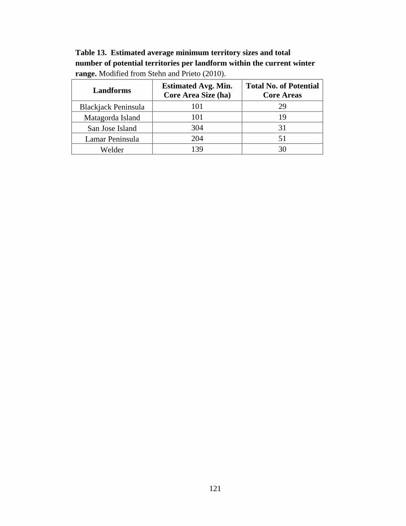
121

Table 13. Estimated average minimum territory sizes and total number of potential territories per landform within the current winter range. Modified from Stehn and Prieto (2010).

Landforms Estimated Avg. Min. Core Area Size (ha)

Total No. of Potential Core Areas

Blackjack Peninsula 101 29 Matagorda Island 101 19 San Jose Island 304 31

Lamar Peninsula 204 51 Welder 139 30

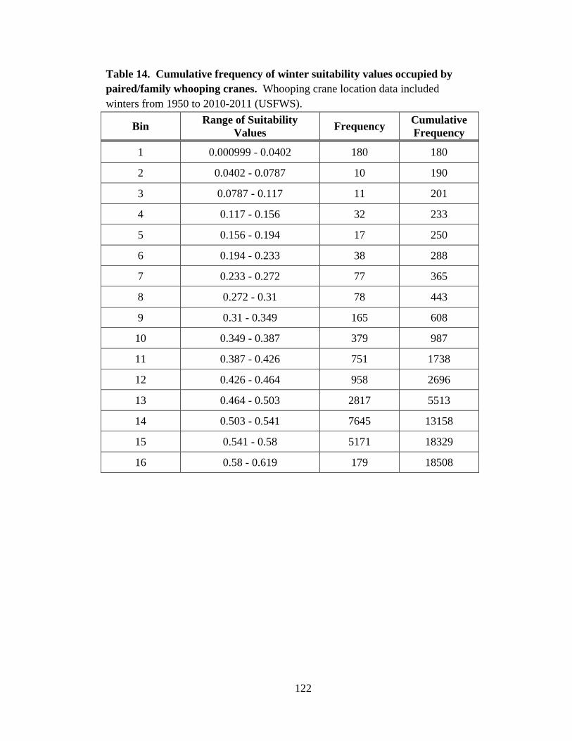
122

Table 14. Cumulative frequency of winter suitability values occupied by paired/family whooping cranes. Whooping crane location data included winters from 1950 to 2010-2011 (USFWS).

Bin Range of Suitability Values Frequency Cumulative

Frequency

1 0.000999 - 0.0402 180 180

2 0.0402 - 0.0787 10 190

3 0.0787 - 0.117 11 201

4 0.117 - 0.156 32 233

5 0.156 - 0.194 17 250

6 0.194 - 0.233 38 288

7 0.233 - 0.272 77 365

8 0.272 - 0.31 78 443

9 0.31 - 0.349 165 608

10 0.349 - 0.387 379 987

11 0.387 - 0.426 751 1738

12 0.426 - 0.464 958 2696

13 0.464 - 0.503 2817 5513

14 0.503 - 0.541 7645 13158

15 0.541 - 0.58 5171 18329

16 0.58 - 0.619 179 18508

123

Table 15. Fixed and Monte Carlo core area sizes and the simulated carrying capacity for each landform. Results are based on a suitability threshold ≥0.426.

Landform

Predicted Carrying Capacity (Stehn &

Prieto 2010)

Fixed Avg. Min.

Territory Sizes (ha)

Fixed Avg. Min.

Territory Sizes

(no. cells)

Simulated Carrying Capacity

(fixed)

Monte Carlo Avg. Core Area

Size (ha)

Monte Carlo

Avg. Core Area Size (no. cells)

Simulated Carrying Capacity

(Monte Carlo)

Blackjack 29 101 1122 35 108 1197 40

Matagorda 51 204 2267 50 232 2377 60

Lamar 19 101 1122 5 110 1224 6

San Jose 31 304 3378 27 378 4204 33

POC 30 139 1544 18 233 2586 20

other - - - - - - -

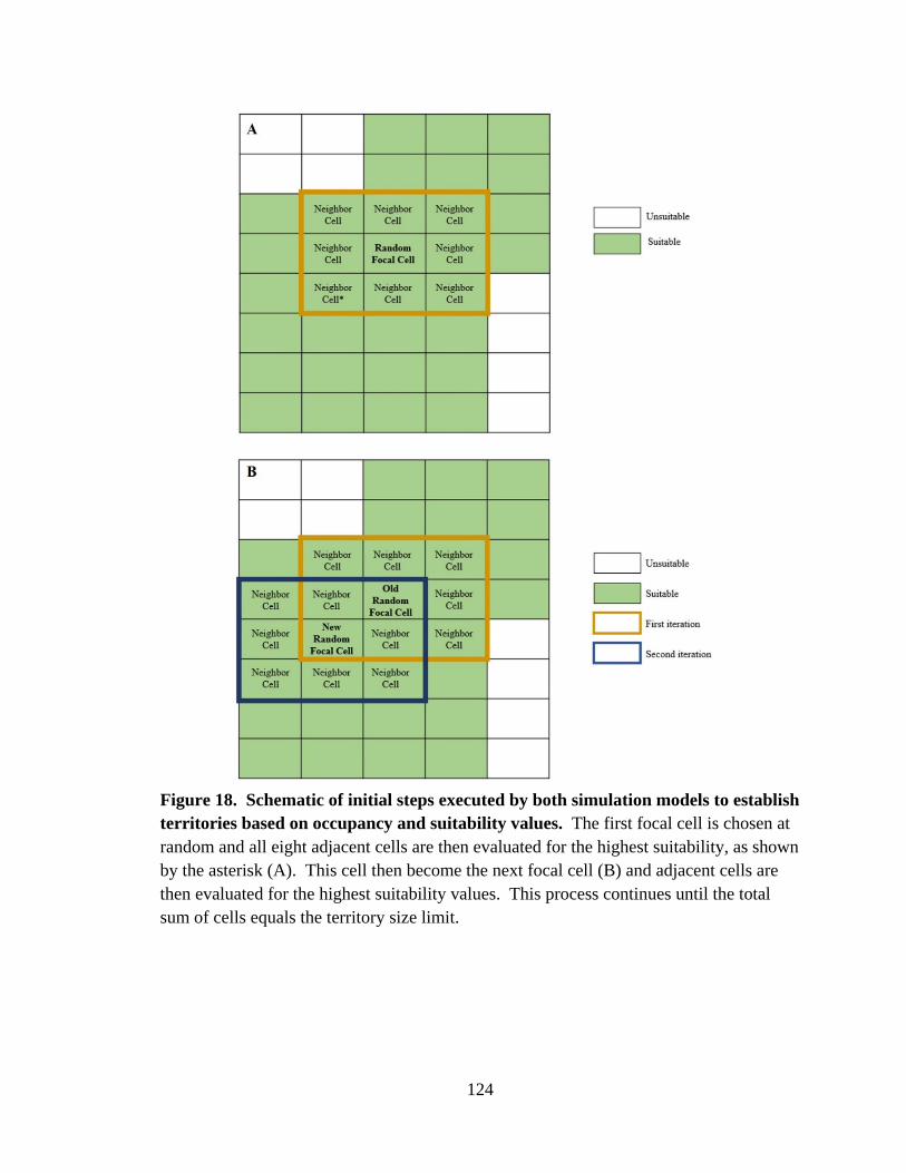
124

Figure 18. Schematic of initial steps executed by both simulation models to establish territories based on occupancy and suitability values. The first focal cell is chosen at random and all eight adjacent cells are then evaluated for the highest suitability, as shown by the asterisk (A). This cell then become the next focal cell (B) and adjacent cells are then evaluated for the highest suitability values. This process continues until the total sum of cells equals the territory size limit.

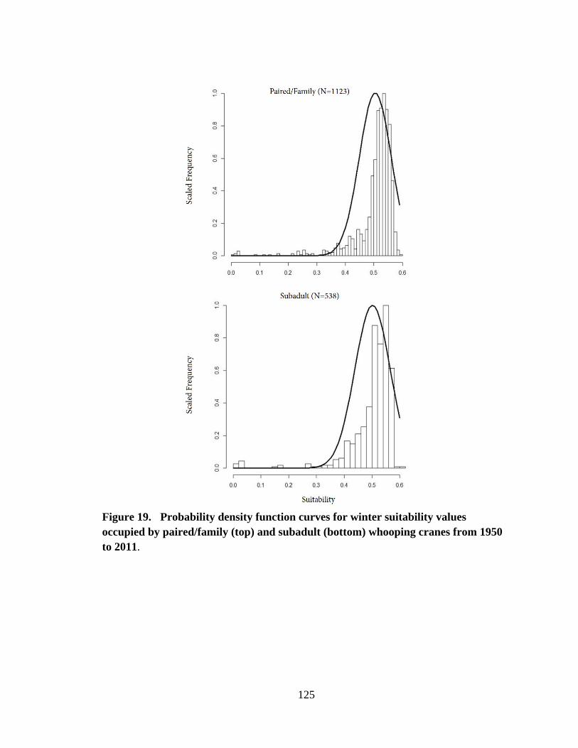
125

Figure 19. Probability density function curves for winter suitability values occupied by paired/family (top) and subadult (bottom) whooping cranes from 1950 to 2011.

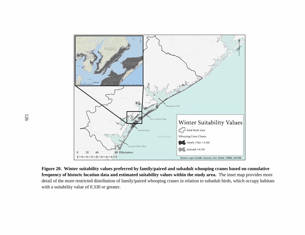
126

Figure 20. Winter suitability values preferred by family/paired and subadult whooping cranes based on cumulative frequency of historic location data and estimated suitability values within the study area. The inset map provides more detail of the more restricted distribution of family/paired whooping cranes in relation to subadult birds, which occupy habitats with a suitability value of 0.330 or greater.

127

Figure 21. Comparison of simulated territories using two different expansion methods in the simulation models. Top - initial expansion of territory into highest suitable cell in next ‘Adjacent’ function resulted in ecologically unrealistic gaps. Bottom – expand territories into the highest suitable cell from stored list of values resulting in most realistic territory development.

128

Figure 22. Simulated whooping crane territories established within the current winter range compared to mapped territories. Note the similarity in structure and extent of the mapped and simulated territories, especially on Blackjack Peninsula where it is suggested territories have met a minimum size constraint.

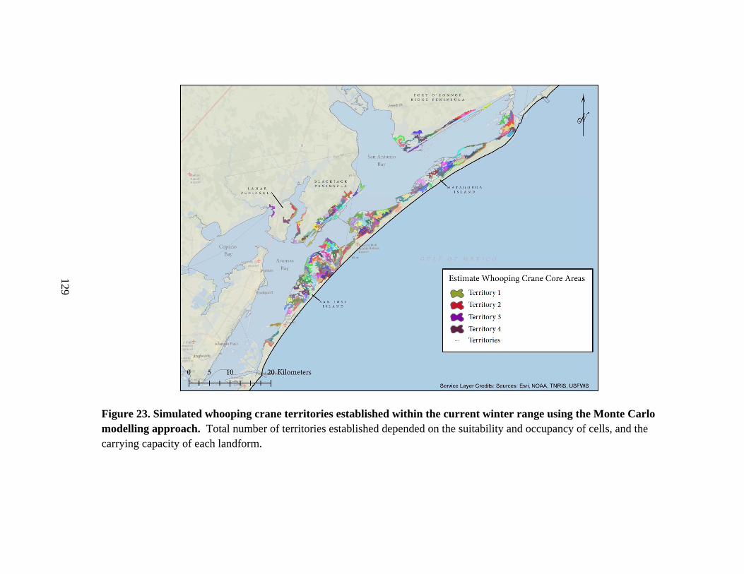
129

Figure 23. Simulated whooping crane territories established within the current winter range using the Monte Carlo modelling approach. Total number of territories established depended on the suitability and occupancy of cells, and the carrying capacity of each landform.

130

Figure 24. Simulated whooping crane territories established on each landform within the current winter range. Note the number of territories established per landform is based on one out of 1,000 simulations ran for each landform to determine the average number of territories that could be established.

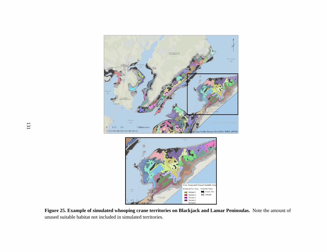
131

Figure 25. Example of simulated whooping crane territories on Blackjack and Lamar Peninsulas. Note the amount of unused suitable habitat not included in simulated territories.

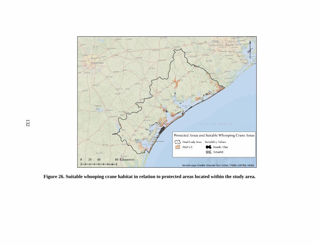
132

Figure 26. Suitable whooping crane habitat in relation to protected areas located within the study area.

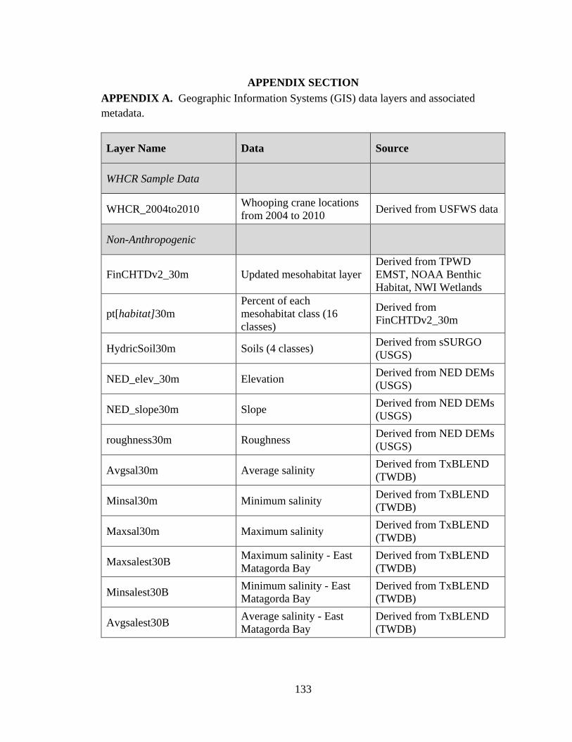
133

APPENDIX SECTION APPENDIX A. Geographic Information Systems (GIS) data layers and associated metadata.

Layer Name Data Source

WHCR Sample Data

WHCR_2004to2010 Whooping crane locations from 2004 to 2010 Derived from USFWS data

Non-Anthropogenic

FinCHTDv2_30m Updated mesohabitat layer Derived from TPWD EMST, NOAA Benthic Habitat, NWI Wetlands

pt[habitat]30m Percent of each mesohabitat class (16 classes)

Derived from FinCHTDv2_30m

HydricSoil30m Soils (4 classes) Derived from sSURGO (USGS)

NED_elev_30m Elevation Derived from NED DEMs (USGS)

NED_slope30m Slope Derived from NED DEMs (USGS)

roughness30m Roughness Derived from NED DEMs (USGS)

Avgsal30m Average salinity Derived from TxBLEND (TWDB)

Minsal30m Minimum salinity Derived from TxBLEND (TWDB)

Maxsal30m Maximum salinity Derived from TxBLEND (TWDB)

Maxsalest30B Maximum salinity - East Matagorda Bay

Derived from TxBLEND (TWDB)

Minsalest30B Minimum salinity - East Matagorda Bay

Derived from TxBLEND (TWDB)

Avgsalest30B Average salinity - East Matagorda Bay

Derived from TxBLEND (TWDB)

134

Appendix A. Continued.

Layer Name Data Source

disttoshrb30m Distance to scrub-shrub (class 7 & 11)

Derived from FinCHTDv2_30m

disttowdy30m Distance to woody (class 12 & 16)

Derived from FinCHTDv2_30m

disttoeow30m Distance to estuarine open water (class 2)

Derived from FinCHTDv2_30m

disttosgrs30m Distance to seagrass (class 6)

Derived from FinCHTDv2_30m

disttoevm30m Distance to estuarine vegetated marsh (class 5)

Derived from FinCHTDv2_30m

disttofw30m Distance to forested wetland (class 8 & 9)

Derived from FinCHTDv2_30m

PatchEcon Fragstats - Edge contrast Derived from FinCHTDv2_30m

PatchContig Fragstats - Patch contiguity Derived from FinCHTDv2_30m

PatchArea Fragstats - Patch area Derived from FinCHTDv2_30m

PatchProx Fragstats - Patch proximity Derived from FinCHTDv2_30m

Anthropogenic

disttodev30m Distance to urban development (class 13)

Derived from FinCHTDv2_30m

avgdensrd30m Average density of roads Derived from TxDOT2015_rd layer from TNRIS

disttord Distance to roads Derived from TxDOT2015_rd layer from TNRIS

Extent (top, left, right, bottom): 7290867.057030, 1692972.272520, 1944192.272520, 7055067.057030 | Number of rows and columns: 8374, 7860

Cell Size: 30, 30 | Projection: NAD83_HARN_Texas_Centric_Albers_Equal_Area (EPSG:3085)

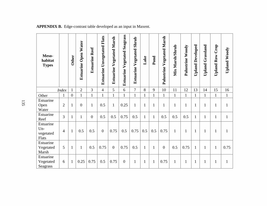
135

APPENDIX B. Edge-contrast table developed as an input in Maxent.

Meso-habitat Types

Oth

er

Est

uari

ne O

pen

Wat

er

Est

uari

ne R

eef

Est

uari

ne U

nveg

etat

ed F

lats

Est

uari

ne V

eget

ated

Mar

sh

Est

uari

ne V

eget

ated

Sea

gras

s

Est

uari

ne V

eget

ated

Shr

ub

Lak

e

Pond

Palu

stri

ne V

eget

ated

Mar

sh

Mix

Mar

sh/S

hrub

Palu

stri

ne W

oody

Upl

and

Dev

elop

ed

Upl

and

Gra

ssla

nd

Upl

and

Row

Cro

p

Upl

and

Woo

dy

Index 1 2 3 4 5 6 7 8 9 10 11 12 13 14 15 16 Other 1 0 1 1 1 1 1 1 1 1 1 1 1 1 1 1 1 Estuarine Open Water

2 1 0 1 0.5 1 0.25 1 1 1 1 1 1 1 1 1 1

Estuarine Reef 3 1 1 0 0.5 0.5 0.75 0.5 1 1 0.5 0.5 0.5 1 1 1 1

Estuarine Un-vegetated Flats

4 1 0.5 0.5 0 0.75 0.5 0.75 0.5 0.5 0.75 1 1 1 1 1 1

Estuarine Vegetated Marsh

5 1 1 0.5 0.75 0 0.75 0.5 1 1 0 0.5 0.75 1 1 1 0.75

Estuarine Vegetated Seagrass

6 1 0.25 0.75 0.5 0.75 0 1 1 1 0.75 1 1 1 1 1 1

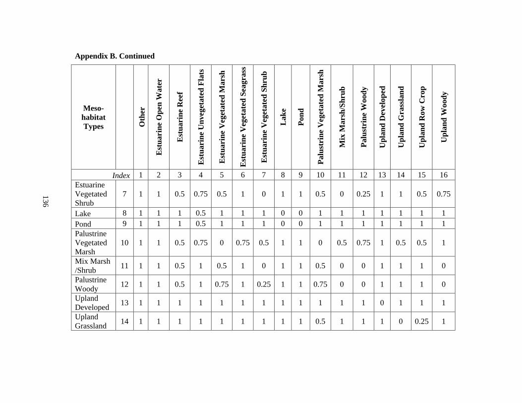
136

Appendix B. Continued

Meso-habitat Types

Oth

er

Est

uari

ne O

pen

Wat

er

Est

uari

ne R

eef

Est

uari

ne U

nveg

etat

ed F

lats

Est

uari

ne V

eget

ated

Mar

sh

Est

uari

ne V

eget

ated

Sea

gras

s

Est

uari

ne V

eget

ated

Shr

ub

Lak

e

Pond

Palu

stri

ne V

eget

ated

Mar

sh

Mix

Mar

sh/S

hrub

Palu

stri

ne W

oody

Upl

and

Dev

elop

ed

Upl

and

Gra

ssla

nd

Upl

and

Row

Cro

p

Upl

and

Woo

dy

Index 1 2 3 4 5 6 7 8 9 10 11 12 13 14 15 16 Estuarine Vegetated Shrub

7 1 1 0.5 0.75 0.5 1 0 1 1 0.5 0 0.25 1 1 0.5 0.75

Lake 8 1 1 1 0.5 1 1 1 0 0 1 1 1 1 1 1 1 Pond 9 1 1 1 0.5 1 1 1 0 0 1 1 1 1 1 1 1 Palustrine Vegetated Marsh

10 1 1 0.5 0.75 0 0.75 0.5 1 1 0 0.5 0.75 1 0.5 0.5 1

Mix Marsh /Shrub 11 1 1 0.5 1 0.5 1 0 1 1 0.5 0 0 1 1 1 0

Palustrine Woody 12 1 1 0.5 1 0.75 1 0.25 1 1 0.75 0 0 1 1 1 0

Upland Developed 13 1 1 1 1 1 1 1 1 1 1 1 1 0 1 1 1

Upland Grassland 14 1 1 1 1 1 1 1 1 1 0.5 1 1 1 0 0.25 1

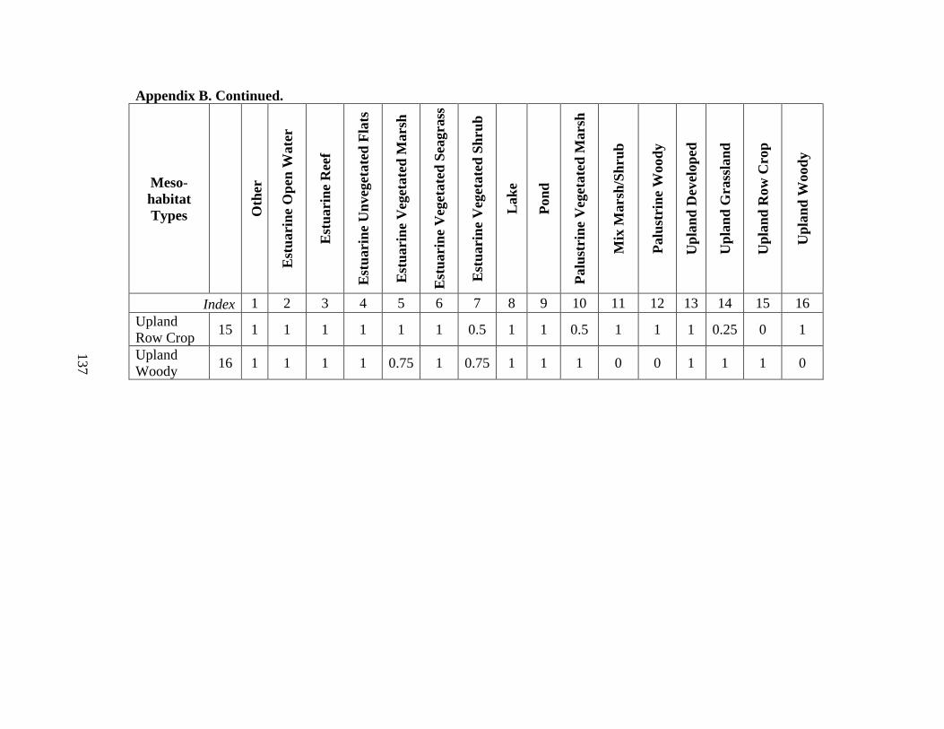
137

Appendix B. Continued.

Meso-habitat Types

Oth

er

Est

uari

ne O

pen

Wat

er

Est

uari

ne R

eef

Est

uari

ne U

nveg

etat

ed F

lats

Est

uari

ne V

eget

ated

Mar

sh

Est

uari

ne V

eget

ated

Sea

gras

s

Est

uari

ne V

eget

ated

Shr

ub

Lak

e

Pond

Palu

stri

ne V

eget

ated

Mar

sh

Mix

Mar

sh/S

hrub

Palu

stri

ne W

oody

Upl

and

Dev

elop

ed

Upl

and

Gra

ssla

nd

Upl

and

Row

Cro

p

Upl

and

Woo

dy

Index 1 2 3 4 5 6 7 8 9 10 11 12 13 14 15 16 Upland Row Crop 15 1 1 1 1 1 1 0.5 1 1 0.5 1 1 1 0.25 0 1

Upland Woody 16 1 1 1 1 0.75 1 0.75 1 1 1 0 0 1 1 1 0

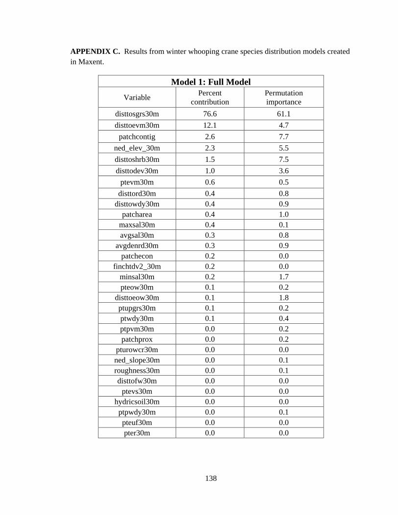
138

APPENDIX C. Results from winter whooping crane species distribution models created in Maxent.

Model 1: Full Model

Variable Percent contribution

Permutation importance

disttosgrs30m 76.6 61.1 disttoevm30m 12.1 4.7

patchcontig 2.6 7.7 ned_elev_30m 2.3 5.5 disttoshrb30m 1.5 7.5 disttodev30m 1.0 3.6

ptevm30m 0.6 0.5 disttord30m 0.4 0.8

disttowdy30m 0.4 0.9 patcharea 0.4 1.0

maxsal30m 0.4 0.1 avgsal30m 0.3 0.8

avgdenrd30m 0.3 0.9 patchecon 0.2 0.0

finchtdv2_30m 0.2 0.0 minsal30m 0.2 1.7 pteow30m 0.1 0.2

disttoeow30m 0.1 1.8 ptupgrs30m 0.1 0.2 ptwdy30m 0.1 0.4 ptpvm30m 0.0 0.2 patchprox 0.0 0.2

pturowcr30m 0.0 0.0 ned_slope30m 0.0 0.1 roughness30m 0.0 0.1 disttofw30m 0.0 0.0

ptevs30m 0.0 0.0 hydricsoil30m 0.0 0.0 ptpwdy30m 0.0 0.1 pteuf30m 0.0 0.0 pter30m 0.0 0.0

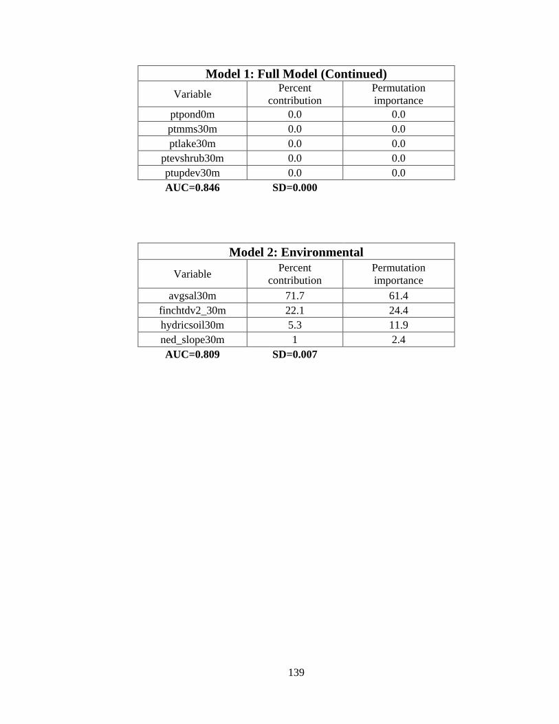
139

Model 1: Full Model (Continued)

Variable Percent contribution

Permutation importance

ptpond0m 0.0 0.0 ptmms30m 0.0 0.0 ptlake30m 0.0 0.0

ptevshrub30m 0.0 0.0 ptupdev30m 0.0 0.0 AUC=0.846 SD=0.000

Model 2: Environmental

Variable Percent contribution

Permutation importance

avgsal30m 71.7 61.4 finchtdv2_30m 22.1 24.4 hydricsoil30m 5.3 11.9 ned_slope30m 1 2.4 AUC=0.809 SD=0.007

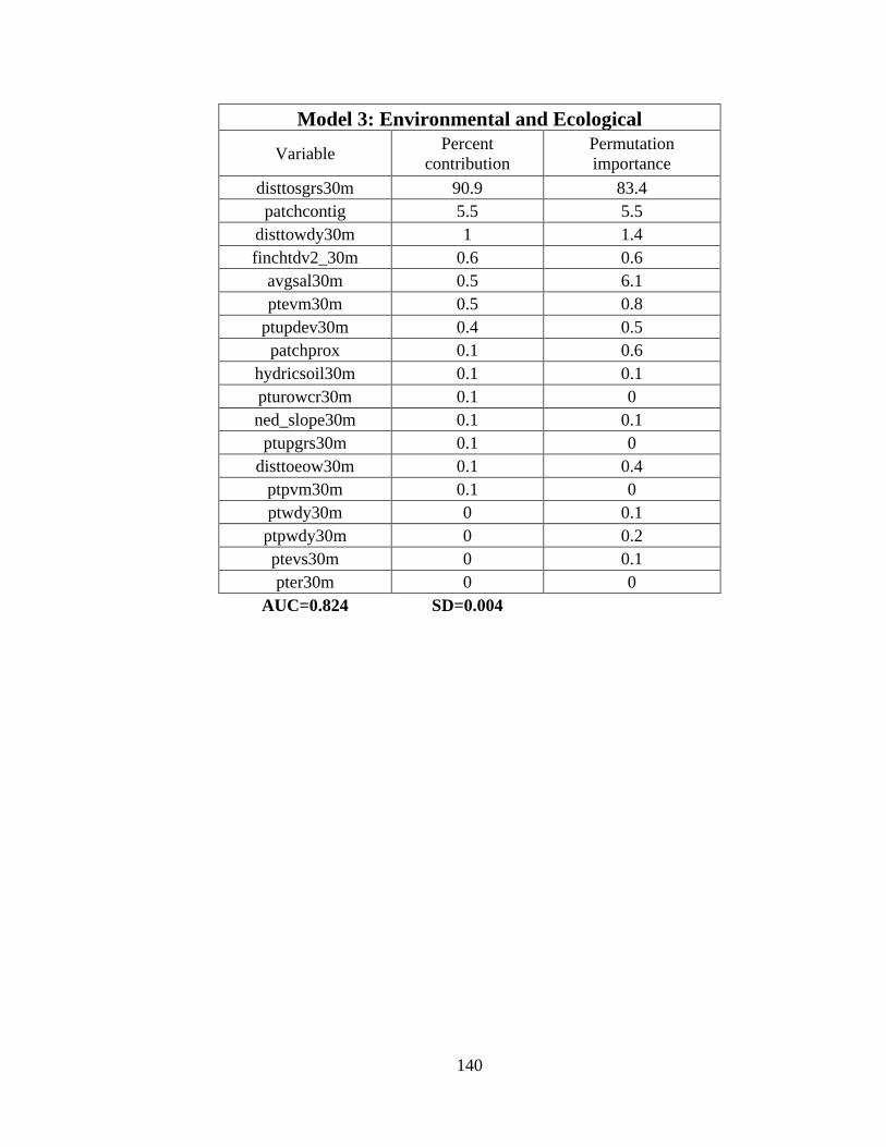
140

Model 3: Environmental and Ecological

Variable Percent contribution

Permutation importance

disttosgrs30m 90.9 83.4 patchcontig 5.5 5.5

disttowdy30m 1 1.4 finchtdv2_30m 0.6 0.6

avgsal30m 0.5 6.1 ptevm30m 0.5 0.8

ptupdev30m 0.4 0.5 patchprox 0.1 0.6

hydricsoil30m 0.1 0.1 pturowcr30m 0.1 0 ned_slope30m 0.1 0.1

ptupgrs30m 0.1 0 disttoeow30m 0.1 0.4

ptpvm30m 0.1 0 ptwdy30m 0 0.1 ptpwdy30m 0 0.2 ptevs30m 0 0.1 pter30m 0 0

AUC=0.824 SD=0.004

141

Model 4: New Full Model Variable Percent

contribution Permutation importance

disttosgrs30m 89.2 84 patchcontig 5.6 3.1

avgdenrd30m 1.3 0.9 disttodev30m 1.3 3.4 disttowdy30m 1 1.6

avgsal30m 0.3 4.5 ptevm30m 0.3 0.5

finchtdv2_30m 0.2 0.6 disttord30m 0.2 0.6

ned_slope30m 0.2 0.1 disttoeow30m 0.1 0.1

ptpvm30m 0.1 0 ptupgrs30m 0.1 0.4

pturowcr30m 0.1 0 patchprox 0 0

hydricsoil30m 0 0 ptwdy30m 0 0 ptevs30m 0 0 pter30m 0 0

ptpwdy30m 0 0 ptupdev30m 0 0 AUC=0.824 SD=0.006

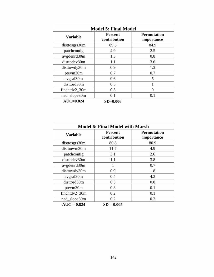
142

Model 5: Final Model Variable Percent

contribution Permutation importance

disttosgrs30m 89.5 84.9 patchcontig 4.9 2.5

avgdenrd30m 1.3 0.8 disttodev30m 1.1 3.6 disttowdy30m 0.9 1.3

ptevm30m 0.7 0.7 avgsal30m 0.6 5 disttord30m 0.5 1

finchtdv2_30m 0.3 0 ned_slope30m 0.1 0.1 AUC=0.824 SD=0.006

Model 6: Final Model with Marsh Variable Percent

contribution Permutation importance

disttosgrs30m 80.8 80.9 disttoevm30m 11.7 4.9

patchcontig 3.1 2.6 disttodev30m 1.1 3.8 avgdenrd30m 1 0.7 disttowdy30m 0.9 1.8

avgsal30m 0.4 4.2 disttord30m 0.3 0.8 ptevm30m 0.3 0.1

finchtdv2_30m 0.2 0.1 ned_slope30m 0.2 0.2 AUC = 0.824 SD = 0.005

143

APPENDIX D

Randomization and Monte Carlo simulation R scripts Author: Nicole A Davis

Editor(s): Thom B. Hardy, Ph.D., Texas State University (Major Professor) and Dorn M. Moore, International Crane Foundation

Author Date: 2018-08-28 Purpose: Develop whooping crane core areas on specific landforms within the winter

range to evaluate carrying capacity and mimic winter range distribution Contact: Nicole Davis (n.davis@txstate.edu OR nadavis2010@gmail.com)

INITIAL R SETUP chooseCRANmirror() install.packages("raster") install.packages("sp") install.packages("rgdal") install.packages("rgeos") install.packages("plyr") install.packages("dplyr") install.packages("ggplot2") install.packages("maptools") install.packages("data.table") install.packages("adehabitatHR") library(raster) library(sp) library(rgdal) library(rgeos) library(plyr) library(dplyr) library(ggplot2) library(maptools) library(data.table) library(adehabitatHR)

144

DEVELOP FUNCTIONS Random Cell Function

Sample a list of suitable cells to choose a suitable and unoccupied focal cell to start

Input: x = raster stack (suitability, occupancy, and unique cell number)

Output: npt = focal cell; randomly chosen suitable and available cell (unique cell number) Script random.sample = function(x){

suitable_cells = x[x[,3] >=suit_limit & x[,4] == 0,] npt = suitable_cells[sample(nrow(suitable_cells), 1), ] return(npt) # Returns suitable cell number

} Neighborhood Function

Sample 8 cells surrounding the focal cell and store available and unoccupied cells in a vector

Input: p = npt (focal cell) and y = raster stack

Output: scv = suitable cell vector; comprised of unique cell numbers

hs = selected cell; unique cell number

Script neighbor1 = function(p, y){

h = adjacent(y, cells = p, directions = 8, pairs = FALSE, target = NULL, sorted= TRUE, include = FALSE, id = TRUE) # look at suitability in adjacent neighborhood h = extract(y, h) # extract values from raster stack - no xy values h2 = merge(data, h, by.x="layer.2", by.y="layer.2") # merge extracted values with data to include xy values hs = subset(h2, suitpdf_na2.x > suit_limit & layer.1.x <= 0, select = c(layer.2, x, y, suitpdf_na2.x, layer.1.x)) # subset data to include only suitable and unoccupied cells scv = c(p, hs[,1]) #store suitable and unoccupied cell id's

145

return(list(hs, scv)) #returns a list with h (all data from dataframe) and scv (cell id's) - query using variable name[1 or 2]

} Expand Territory

Use the highest suitable cell from the suitable cell vector that is different than the already selected focal cell and continue the neighborhood function to grow the core area

Input: run1 = results from the neighborhood function; unique cell numbers of cells surrounding focal cell

Rca = random core area size (Monte Carlo simulation only); total number of cells

Stack = raster stack

Cc = cell count; track number of cells comprising the core area

Scv = suitable cell vector

Selected = selected cell vector; unique cell numbers of focal cells

Birdit = unique bird ID; each iteration is considered to be one pair of whooping cranes

Output: ca = list of unique cell numbers that comprise core area for Birdit

Script expand_core_area = function(run1, rca, stack, cc, scv, selected, birdit){

list = run1[1] #store values from adjacent function in a list hood1 = ldply(list, data.frame) # convert list to dataframe next_cell = hood1[,1][which(hood1[,4] == max(hood1[,4]))] # choose the next cell from 1st neighborhood while(cc >= 0 && cc < rca){ #stay in loop until reach core area size

#Look at next neighborhood for new focal cell nrbh = adjacent(stack, cells = c(next_cell), directions=8, pairs = FALSE, target = NULL, sorted = TRUE, include = FALSE, id = TRUE) new_nrbh = setdiff(nrbh, scv) n = extract(stack, new_nrbh) n2 = merge(data, n, by.x="layer.2", by.y="layer.2")

146

n3 = (subset(n2, suitpdf_na2.x > suit_limit & layer.1.x <= 0, select = c(layer.2, x, y, suitpdf_na2.x, layer.1.x))) scv = union(scv, n3[,1]) #add new suitable and available cells to scv #duplicated(scv) #check for duplicate values selected = unique(c(selected, next_cell)) #add newly selected focal cell to selected cc = length(scv) #keep track of the total number of cells of core area

#Check if scv equals selected if(length(scv) != length(selected)){ #If not equal, then

available = setdiff(scv, selected) # look at available cells that have not been selected

scv_hood = extract(stack, available) #get suitability values for available cells

new_cell = scv_hood[,3][which(scv_hood[,1] == max(scv_hood[,1]))] #selected next focal cell #print(paste("chose an available cell: ", new_cell)) #break

} else { repeat {

new_cell = (random.sample(data))[,5] #if equal, then go to a new random cell and start over adjcells = adjacent(stack, cells = new_cell, directions = 8, pairs = FALSE, target = NULL, sorted = TRUE, include = FALSE, id = TRUE) adjcells2 = data.frame(extract(stack, adjcells)) adjsub = subset(adjcells2, adjcells2[,1] > suit_limit & adjcells2[,2] == 0) if(nrow(adjsub) > 0) break #if no suitable cells surrounding new focal cell, repeat random cell selection

} #set occupancy values to 9999 for cells that could not make a core area in above step

stack[[2]] [stack[[3]] %in% c(scv)] = 9999 scv = c() #clear suitable cell vector when bird moves selected = c() #clear selected cell vector when bird moves birdit = birdit + 1 plot(stack[[2]])

147

print(paste("all available cells chosen; had to move: ", new_cell)) #break

} next_cell = new_cell cc = length(scv) if(birdit > 25){ print("Bird jumped more than 25 times") break #stop model if bird jumps more than 25 times } }

ca = (list(scv, next_cell, selected, cc, birdit)) #need scv and next_cell to continue analysis

}

CREATE VARIABLES Create connections to pathways and files to allow the user to provide study area input

Input: pathnames and area; user will type in study area; i.e., landform

Script study_area = function(area){

# SelectStudyArea() sets specific global variables (<<-) if(area == "blackjack") {

setwd("pathname") shp <<- readOGR("pathname\\Blackjack_peninsula.shp") rcaoutfile <<- "Blackjack_Core_Area_Sizes.csv" rcapath <<- file.path("C:","Blackjack",rcaoutfile) N <<- 100 #total number of birds that could be on landscape using smallest core area size total_area <<- 54244 #total no. of suitable cells mn <<- 1178 sd <<- 475 # rca <<- abs(round(rnorm(1, 1178, 475),digits=0)) #for Monte Carlo

} else if (area == "lamar") {

setwd("C:\\pathname") shp <<- readOGR("C:\\pathname\\Lamar_peninsula.shp")

148

rcaoutfile <<- "Lamar_Core_Area_Sizes.csv" rcapath <<- file.path("C:","Lamar",rcaoutfile) N <<- 100 #total number of birds that could be on landscape using smallest core area size total_area <<- 10097 #total no. of suitable cells mn <<- 1217 sd <<- 320 # rca <<- abs(round(rnorm(1, 1217, 320),digits=0)) #for Monte Carlo

} else if (area == "matagorda") {

setwd("C:\\pathname") shp <<- readOGR("C:\\pathname\\Matagorda_Island.shp") rcaoutfile <<- "Matagorda_Core_Area_Sizes.csv" rcapath <<- file.path("C:","Matagorda",rcaoutfile) N <<- 200 #total number of birds that could be on landscape using smallest core area size total_area <<- 150422 #total no. of suitable cells mn <<- 2346 sd <<- 927 # rca <<- abs(round(rnorm(1, 2346, 927),digits=0)) #for Monte Carlo

} else if (area == "other"){

setwd("C:\\pathname") shp <<- readOGR("C:\\pathname\\other.shp") rcaoutfile <<- "Other_Core_Area_Sizes.csv" rcapath <<- file.path("C:","Other",rcaoutfile) N <<- 800 #total number of birds that could be on landscape using smallest core area size total_area <<- 536852 #total no. of suitable cells mn <<- 1178 sd <<- 475 # rca <<- abs(round(rnorm(1, 1178, 475),digits=0))

} else if (area == "sanjose"){

setwd("C:\\Users\\admin\\Documents\\TSU_Dissertation\\Dissertation Documents\\GIS\\NIKKI") shp <<-

149

readOGR("C:\\Users\\admin\\Documents\\TSU_Dissertation\\Dissertation Documents\\GIS\\NIKKI\\landforms\\SanJose_Island.shp") rcaoutfile <<- "SanJose_Core_Area_Sizes.csv" rcapath <<- file.path("C:","SanJose",rcaoutfile) N <<- 100 #total number of birds that could be on landscape using smallest core area size total_area <<- 126325 #total no. of suitable cells mn <<- 4002 sd <<- 2267 #rca <<- abs(round(rnorm(1, 4002, 2267),digits=0)) #for Monte Carlo

} else if (area == "poc"){

setwd("C:\\Users\\admin\\Documents\\TSU_Dissertation\\Dissertation Documents\\GIS\\NIKKI") shp <<- readOGR("C:\\Users\\admin\\Documents\\TSU_Dissertation\\Dissertation Documents\\GIS\\NIKKI\\landforms\\PortO_peninsula.shp") rcaoutfile <<- "POC_Core_Area_Sizes.csv" rcapath <<- file.path("C:","PortO",rcaoutfile) N <<- 100 #total number of birds that could be on landscape using smallest core area size total_area <<- 47732 #total no. of suitable cells mn <<- 2576 sd <<- 1567 # rca <<- abs(round(rnorm(1, 2576, 1567),digits=0)) #for Monte Carlo

} else {

stop("The study area you provided is not in the list.") break }

}

150

ANALYSIS SCRIPT # Set the Suitability Value threshhold suit_limit = 0.426 #minimum suitability value for paired/family birds # REQUIRED FROM USER- Provide the study area name as a variable. # options are : # 'blackjack', 'lamar', 'matagorda', 'other', 'poc', 'sanjose' # e.g. study_area("blackjack") study_area("") # Set the suitability raster - should be in the Working Directory # print(getwd()) suit = raster("suitpdf_na2") #reclassified suitability raster raster = crop(suit, shp) occupr = raster(raster) occupr = setValues(raster(occupr), occupr[]) #remove attributes from raster occupr = crop(occupr, shp) sa = mask(raster, shp) saoccupr = mask(occupr, shp) cells = raster(sa) values(cells) = 1:ncell(cells) sa[is.na(sa[])] = 0 #set NAs to 0 saoccupr[is.na(saoccupr[])] = 0 #set NAs to 0 stack = stack(sa, saoccupr, cells) data = data.frame(rasterToPoints(stack)) #full dataset data = subset(data, data[,3] >= suit_limit) #reduced data by suitability #plot(stack) #Start Simulation system.time({

for(i in 1:5){ stack = stack(sa, saoccupr, cells) data = data.frame(rasterToPoints(stack)) data = subset(data, data[,3] >= suit_limit & data[,4] ==0) birdID = 1

151

area_tracker = 0 # keep track of area occupied as more bird make core areas (# of cells) birdit = 0 rca = abs(round(rnorm(1, mn, sd),digits=0)) # randomized core area size

while(birdID <= N){

while(area_tracker <= total_area){ # repeat loop - randomly select suitable cell, if occupied, repeat random selection repeat{

newpt = random.sample(data) # random cell from list of suitable cells zz = paste(birdID, newpt[,5], sep=" ") run1 = neighbor1(newpt[,5], stack) run1df = run1[[1]] if(nrow(run1df) > 0){

selected = newpt[,5] # stores random cell as 1st selected cell break

} else{ break

} }

scv = c(newpt[,5],unlist(run1[[1]][,1], use.names=FALSE)) # stores random cell and surrounding suitable cells in suitable cell vector - available cells cc = (length(scv)) # stores total number of cells - once reach 1124, core area complete, and go to next bird ca = expand_core_area(run1, rca, stack, cc, scv, selected, birdit) # create core area by expanding from initial cell outward, 8-cell neighbors z = length(ca[[1]]) if(z >= rca){ caoutfile = paste("CoreArea_Bird_", birdID, "_M", i, ".csv",sep="") #create core area from expand() - creates list with 2 lists - scv cell IDs and next cell write.table(ca[[1]], file=caoutfile, append=TRUE, col.names=FALSE, row.names=FALSE) stack[[2]][stack[[3]] %in% c(ca[[1]])] = birdID #update occupancy values using birdID data = data.frame(rasterToPoints(stack)) #update data dataframe to show occupied cells data = subset(data, data[,3] >= suit_limit & data[,4] == 0)

area_tracker = sum(c(area_tracker, ca[[4]])) #add up total core area cells

152

print(paste("Bird ID: ", birdID, " cc= ", length(ca[[1]]))) birdID = birdID + 1 break } else{ break } } if(ca[[5]] > 25){ print(paste(birdID, " did not make core area")) break } if(area_tracker>=total_area) break } print(paste("Total area: ", area_tracker, " No. Birds: ", birdID)) write.table(rbind(rca,birdID),file=rcapath, append=TRUE, sep=",",col.names=FALSE,row.names=FALSE) } #Close the for loop })

153

LITERATURE CITED Abdi, H. and Williams, L.J. 2010. Principal component analysis. WIREs Computational

Statistics 2:433-459.

Adair, S.E., Moore, J.L. and Onuf, C.P. 1994. Distribution and status of submerged

vegetation in estuaries of the upper Texas coast. Wetlands 14:110-121.

Adams, E.S. 2001. Approaches to the study of territory size and shape. Annual Review

of Ecology and Systematics 32:277-303.

Akaike, H. 1974. A new look at the statistical model identification. IEEE Transactions

on Automatic Control 19:716-723.

Allen, R.P. 1952. The Whooping Crane. New York: New York, National Audubon

Society, Research Report No. 3, 246pp.

Alonso, J.C., Alonso, J.A., Bautista, L.M. and Muñoz-Pulido, R. 1995. Patch use in

cranes: a field test of optimal foraging predictions. Animal Behavior 49:1367-

1379.

Alonso, J.C., Bautista, L.M. and Alonso, J.A. 2004. Family-based territoriality vs

flocking in wintering common cranes Grus grus. Journal of Avian Biology

35:434-444.

Anderson, D.P., Forester, J.D., Turner, M.G., Frair, J.L., Merrill, E.H., Fortin, D., Mao,

J.S. and Boyce, M.S. 2005. Factors influencing female home range sizes in elk

(Cervus elaphus) in North American landscapes. Landscape Ecology 20:257-271.

Anderson, R.P. and Gonzalez, I. Jr. 2011. Species-specific tuning increases robustness

to sampling bias in models of species distributions: an implementation with

Maxent. Ecological Modelling 222:2796-2811.

154

Angelieri, C.C.S., Adams-Hosking, C., Paschoaletto, K.M., Ferraz, M.B., Souza, M.P. and

McAplina, C.A. 2016. Using species distribution models to predict potential

landscape restoration effects on puma conservation. PLoSONE 11:1-18.

Anich, N.M, Benson, T.J. and Bednarz, J.C. 2009. Estimating territory and home-range

sizes: do singing locations alone provide an accurate estimate of space use? The

Auk 126:626-634.

Archibald, G.W. 1975. The evolutionary and taxonomic relationships of cranes as

revealed by their unison calls. Ithaca, New York: Cornell University, Ph.D. thesis,

151pp.

Armbruster, M.J. 1990. Characterization of habitat used by whooping crane during

migration. U.S. Fish and Wildlife Service, Biological Report 90, 16pp.

Austin, J. and Richert, A. 2005. Patterns of habitat use by whooping cranes during

migration: summary from 1977-1999 site evaluation data. In Proceedings of the

Ninth North American Crane Workshop. (ed.), 79-104.

Baldwin, R.A. 2009. Use of maximum entropy modeling in wildlife research. Entropy

11:854-866.

Baldwin, R.A. and Bender, L.C. 2008. Den-site characteristics of black bears in Rocky

Mountain national park, Colorado. Journal of Wildlife Management 72:1717-

1724.

Barg, J.J., Jones, J. and Robertson, R.J. 2005. Describing breeding territories of

migratory passerines: suggestions for sampling, choice of estimator, and

delineation of core area. Journal of Animal Ecology 74:139-149.

155

Bennett, L.A. and Bennett, A.J. 1992. Territorial behavior of Florida sandhill cranes in

the Okefenokee Swamp. In North American Crane Workshop Proceedings 259

(ed.), 177-184.

Bishop, M.A. and Blankenship, D.R. 1981. Dynamics of subadult flocks of whooping

cranes at Aransas National Wildlife Refuge, Texas, 1979-1981. In Proceedings of

the North American Workshop (ed.), 180-189.

Bishop, A., Liske-Clarke, J., Tacha, M. and Reker, R. 2010. Whooping crane

conservation plan for the Rainwater Basin region of South Central Nebraska:

summary. Rainwater Basin Joint Venture (RWBJV) Report. DOI:

10.13140/RG.2.1.2696.7926. 15pp.

Blankenship, D.R. 1976. Studies of whooping cranes on the wintering grounds. In

Proceedings of the 1976 International Crane Workshop (ed.), 197-206.

Bonds, C.J. 2000. Characterization of Banded Whooping Crane Winter Territories from

1992-93 to 1996-97 Using GIS and Remote Sensing. Master’s Thesis: Texas

A&M University, College Station, Texas. 106pp.

Borger, L., Franconi, N., De Michele, G., Gantz, A., Meschi, F., Manica, A., Lovari, S.

and Coulson, T. 2006. Effects of sampling regime on the mean and variance of

home range size estimates. Journal of Animal Ecology 75:1393-1405.

Boyce, M.S. 1987. Time-series analysis and forecasting of the Aransas/Wood Buffalo

Whooping Crane population. In Proceedings of the International Crane

Workshop 4 (ed.), 1-9.

Boyce, M.S. 2005. Factors influencing female home range sizes in elk (Cervus elaphus)

in North American landscapes. Landscape Ecology 20:257-271.

156

Bradley, B.A., Olsson, A.D., Wang, O., Dickson, B.G., Pelech, L., Sesnie, S.E. and

Zachmann, L.J. 2012. Species detection vs. habitat suitability: are I biasing

habitat suitability with remotely sensed data? Ecological Modelling 244:57-64.

Brook, B.W., Cannon, J.R., Lacy, R.C., Mirande, C. and Frankham, R. 1999.

Comparison of the population viability analysis packages GAPPS, INMAT,

RAMAS and VORTEX for the whooping crane (Grus americana). Animal

Conservation 2:23-31.

Buckman-Sewald, J., Whorton, C.R. and Root, K.V. 2014. Developing macrohabitat

models for bats in parks using maxent and testing them with data collected by

citizen scientists. International Journal of Biodiversity and Conservation 6:171-

183.

Burgman, M.A. and Fox, J.C. 2003. Bias in species range estimates from minimum

convex polygons: implications for conservation and options for improved

planning. Animal Conservation 6:19-28.

Burnham, K.P. and Anderson, D.R. 2002. Model Selection and Mutimodel Inference. A

Practical Information-theoretical Approach. Berlin:Springer. 488pp.

Burt, W.H. 1943. Territoriality and home range concepts as applied to mammals.

Journal of Mammalogy 24:346-352.

Butler, M.J. and Harrell, W. 2018. Whooping Crane Survey Results: Winter 2017-2018.

U.S. Fish and Wildlife Service, Albuquerque, New Mexico, USA. 6pp. Available

from

https://www.fws.gov/uploadedFiles/WHCR%20Update%20Winter%202017-

2018(1).pdf.

157

Butler, M.J., Metzger, K.L. and Harris, G.M. 2017. Are whooping cranes destined for

extinction? Climate change imperils recruitment and population growth. Ecology

and Evolution 7:2821-2834. Available from https://doi.org/10.1002/ece3.2892.

Butler, M.J., Metzger, K.L. and Harris, G.M. 2014. Whooping crane demographic

responses to winter drought focus conservation strategies. Biological

Conservation 179:72-85.

Butler, M.J., Harris, G. and Strobel, B.N. 2013. Influence of whooping crane population

dynamics on its recovery and management. Biological Conservation 162:89-99.

Call, D.R., Gutierrez, R.J. and Verner, J. 1992. Foraging habitat and home-range

characteristics of California spotted owls in the Sierra Nevada. The Condor

94:880-888.

Campioni, L., del Mar Delgado, M., Lourenco, R., Bastianelli, G., Fernandez, N. and

Penteriani, P. 2013. Individual and spatio-temporal variations in the home range

behavior of a long-lived, territorial species. Oecologia 172:371-385.

Canadian Wildlife Service & U. S. Fish and Wildlife Service (CWS and USFWS). 2007.

International Recovery Plan for the Whooping Crane (Grus Americana), Third

Revision. Albuquerque, New Mexico: Recovery of Nationally Endangered

Wildlife (RENEW) and U.S. Fish and Wildlife Service, 162pp.

Cao, Y., DeWalt, R.E., Robinson, J.L., Tweddale, R., Hinz, L. and Pessimo, M. 2013.

Using Maxent to model the historic distribution of stonefly species in Illinois

streams: the effects of regularization and threshold selections. Ecological

Modelling 259:30-39.

158

Caughley, G. and Sinclair, A.R.E. 1994. Wildlife Ecology and Management. Blackwell

Science, Cambridge, Massachusetts, 305pp.

Chavez-Ramirez, F. 1996. Food availability, foraging ecology, and energetics of

whooping cranes wintering in Texas. College Station, Texas: Texas A&M

University, Ph.D. thesis. 103pp.

Chavez-Ramirez, F. and Wehtje, W. 2012. Potential impact of climate change scenarios

on whooping crane life history. Wetlands 32:11-20.

Coates, P.S., Casazza, M.L., Brussee, B.E., Ricca, M.A., Gustafson, K.B., Overton, C.T.,

Sanchez-Chopitea, E., Kroger, T., Mauch, K., Niell, L., Howe, K., Gardner, S.,

Espinosa, S. and Delehanty, D.J. 2014. Spatially Explicit Modeling of Greater

Sage-Grouse (Centrocercus urophasianus) Habitat in Nevada and Northeastern

California—A Decision-Support Tool for Management. Reston, Virginia: U.S.

Department of the Interior and U.S. Geological Survey, U.S. Geological Survey

Open-File Report 2014-1163, 83pp.

Coughenour, M.B. 2002. Elk in the Rocky Mountain National Park Ecosystem – A

Model-based Assessment. Natural Resource Ecology Laboratory, Colorado State

University, Fort Collins, Colorado. 139pp.

Dahle, B., Stoen, O.G. and Swenson, J.E. 2006. Factors influencing home-range size in

subadult brown bears. Journal of Mammalogy 87:859-865.

Di Stefano, J., Coulson, G., Greenfield, A. and Swan, M. 2011. Resource heterogeneity

influences home range area in the swamp wallaby Wallabia bicolor. Ecography

34:469-479.

159

Drew, G.S., Piatt, J.F. and Hill, D.F. 2013. Effects of currents and tides on fine-scale use

of marine bird habitats in a southeast Alaska hotspot. Marine Ecology Progress

Series 487:275-286.

Dunton, K.H., Pulich W. and Mutchler, T. 2010. A Seagrass Monitoring Program for

Texas Coastal Waters: Multiscale Integration of Landscape Features with Plant

and Water Quality Indicators. Corpus Christi, Texas: Coastal Bend Bays and

Estuaries Program, Final report (contract no. 0627), 39pp.

Elith, J. and Leathwick, J.R. 2009. Species distribution models: ecological explanation

and prediction across space and time. Annual Review of Ecology, Evolution, and

Systematics 40:677-697.

Elith, J., Phillips, S.J., Hastie, T., Dudik, M. and Chee, Y.E. 2011. A statistical

explanation of MaxEnt for ecologists. Diversity and Distributions 17:43-57.

Environment Canada. 2007. Recovery strategy for the whooping crane (Grus

americana) in Canada. Species at Risk Act Recovery Strategy Series (vii).

Environment Canada, Ottawa. 27pp.

ESRI. 2011. ArcGIS Desktop: Release 10.1. Redland, CA: Environmental Systems

Research Institute.

Farmer, A.H., Cade, B.S., Terrell, J.W., Henriksen, J.H. and Runge, J.T. 2005.

Evaluation of models and data for assessing whooping crane habitat in the central

Platte River, Nebraska. U.S. Geological Survey, Scientific Investigations Report

2005-5123, 64pp. Access from https://pubs.er.usgs.gov/publication/sir20055123.

Franklin, J. 2010. Moving beyond static species distribution models in support of

conservation biogeography. Diversity and Distributions 16:321-330.

160

Gallien, L., Munkemuller, T., Albert, C.H., Boulangeat, I. and Thuiller, W. 2010.

Predicting potential distributions of invasive species: where to go from here?

Diversity and Distributions 16:331-342.

Gergely, K.J. and McKerrow, A. 2016. PAD-US—National inventory of protected areas

(ver. 1.1, August 2016): U.S. Geological Survey Fact Sheet 2013–3086, 2pp.

Accessed from https://pubs.usgs.gov/fs/2013/3086/.

Gils, H.V., Conti, F., Ciaschetti, G. and Westinga, E. 2012. Fine resolution distribution

modeling of endemics in Majella National Park, Central Italy. Plant Biosystems

146:276-287.

Gils, H.V. Westinga, E., Carafa, M. Antonucci, A. and Ciaschetti, G. 2014. Where the

bears roam in Majella National Park, Italy. Journal for Nature Conservation 22:

23-34.

Gil-Weir, K.C. 2006. Whooping crane (Grus americana) demography and

environmental factors in a population growth simulation model. College Station,

Texas A&M University: Ph.D. thesis, 159pp.

Gil-Weir, K.C., Grant, W.E., Slack, R.D., Wang, H. and Fujiwara, M. 2012.

Demography and population trend of whooping cranes. Journal of Field

Ornithology 83:1-10. Doi:10.1111/j.1557-9263.2011.00349.x

Goetz, S.J., Jantz, P. and Jantz, C.A. 2009. Connectivity of core habitat in the

Northeastern United States: Parks and protected areas in a landscape context.

Remote Sensing of the Environment 113:1421-1429.

161

Greer, D.M. 2010. Blue Crab Population Ecology and Use by Foraging Whooping

Cranes on the Texas Gulf Coast. College Station, Texas: Texas A&M University,

Ph.D. dissertation, 294pp.

Gregory, R.D., Gibbons, D.W. and Donald, P.F. 2004. Bird census and survey

techniques. In: Bird Ecology and Conservation: A Handbook of Techniques (ed.)

W.J. Sutherland, I. Newton, and R.E. Green. Oxford; New York: Oxford

University Press. 386pp.

Gschweng, M., Kalko, E.K.V., Berthold, P., Fiedler, W. and Fahr, J. 2012. Multi-

temporal distribution modeling with satellite tracking data: predicting responses

of a long-distance migrant to changing environmental conditions. Journal of

Applied Ecology 49:803-813.

Guthrie, C.G., Matsumoto, J. and Lu, Q. 2010a. TxBLEND Model Validation for the

Upper Guadalupe Estuary using Recently Updated Inflow Data. Austin, Texas:

Texas Water Development Board, 25pp.

Guthrie, C.G., Matsumoto, J. and Lu, Q., 2010b. TxBLEND Model Calibration and

Validation for the Guadalupe and Mission-Aransas Estuaries. Austin, Texas:

Texas Water Development Board, 46pp.

Haley, D.E. 1987. Drinking sites and requirements of wintering sandhill cranes. In

Proceedings of the 1985 Crane Workshop (ed.), 172-179.

Hamlin, L. 2005. The abundance and spatial distribution of blue crabs (Callinectes

sapidus) in the Guadalupe estuary related to low freshwater inflow conditions.

San Marcos, Texas State University: Master’s thesis. 103pp.

162

Hijman, R.J., Cameron, S.E., Parra, J.L., Jones, P.G. and Jarvis, A. 2005. Very high

resolution interpolated climate surfaces for global land areas. International

Journal of Climatology 25:1965-1978.

Horne, J.S. and E.O. Garton. 2006. Selecting the best home range model: an

information-theoretic approach. Ecology 87:1146-1152.

Hoss, S.K., Guyer, C., Smith, L.L. and Schuett, G.W. 2010. Multiscale influences of

landscape composition and configuration on the spatial ecology of eastern

diamond-backed rattlesnakes (Crotalus adamanteus). Journal of Herpetology

44:110-123.

Howe, M.A. 1987. Habitat use by migrating whooping cranes in the Aransas-Wood

Buffalo corridor. In Proceedings of the North America Crane Workshop (ed.),

303-311.

Howlin, S., Derby, C. and Strickland, D. 2008. Whooping crane migrational habitat use

in the Central Platte River during the Cooperative Agreement Period, 2001-2006.

Western Ecosystem Technology, Inc. Cheyene, Wyoming. 87pp.

Hunt, H.E. and Slack, R.D. 1987. Winter foods of the Whooping Crane based on

stomach content analysis. In Proceedings of the 1985 Crane Workshop (ed.), 217-

218.

Hurler, C., Plucinsky, A. and Nazari R. 2015. Using NOAA SLOSH to Determine

Infrastructural Effects of Coastal Storm Surges: A Technical Report. Rowan

University. Accessed from

http://users.rowan.edu/~nazari/pdf%20files/NOAA%20SLOSH%20Manual.pdf.

163

International Crane Foundation (ICF). 2018. All the whooping cranes in the world.

Access from https://www.savingcranes.org/species-field-guide/whooping-crane/.

Jelesnianski, C.P., Chen, J. and Shaffer, W.A. 1992. SLOSH: Sea, Lake, and Overland

Surges from Hurricanes. Arlington, Virginia: National Oceanographic and

Atmospheric Administration, Technical Report National Weather Service 48,

71pp.

Jiguet, F., Barbet-Massin, M. and Chevallier, D. 2011. Predictive distribution models

applied to satellite tracks: modelling the western African winter range of

European migrant Black Storks Ciconia nigra. Journal of Ornithology 152:111-

118.

Jimenez-Valverde, A. and Lobo, J.M. 2007. Threshold criteria for conversion of

probability of species presence to either-or presence-absence. ACTA Oecologica

31:361-369.

Kesler, D.C. 2012. Foraging habitat distributions affect territory size and shape in the

Tuamotu kingfisher. International Journal of Zoology 2012; article ID 632969;

7p. Doi:10.1155/2012/632969

Khosravi, R., Hemami, M., Malekian, M., Flint, A.L. and Flint, L.E. Maxent modeling

for predicting potential distribution of goitered gazelle in central Iran: the effect of

extent and grain size on performance of the model. Turkish Journal of Zoology

40:574-585.

Kuyt, E. 1979. Banding of juvenile whooping cranes on the breeding range in the

Northwest Territories, Canada. North American Bird Bander 4:24-25.

164

Kuyt, E. 1992. Aerial radio-tracking of Whooping cranes migrating between Wood

Buffalo National Park and Aransas National Wildlife Refuge, 1981-84. Canadian

Wildlife Service Occasional Paper Number 74, Ottawa, Ontario, Canada, 53pp.

Kuyt, E. 1993. Whooping crane, Grus Americana, home range and breeding range

expansion in Wood Buffalo National Park, 1970-1991. The Canadian Field-

Naturalist 107:1-12.

LaFever, K.E. 2006. Spatial and temporal winter territory use and behavioral response

of whooping cranes to human activities. College Station, Texas A&M University:

Master’s thesis. 100pp.

Larson, M.A., Thompson, F.R. III, Millspaugh, J.J., Dijak, W.D. and Shifley S.R. 2004.

Linking population viability, habitat suitability, and landscape simulation models

for conservation planning. Ecological Modelling 180:103-118.

Latif, Q.S., Saab, V.A., Mellen-Mclean, K. and Dudley, J.G. 2015. Evaluating habitat

suitability models for nesting white-headed woodpeckers in unburned forest. The

Journal of Wildlife Management 79:263-273.

Lumb, L.M. 2014. Identifying Habitat Conservation Needs for the Endangered

Whooping Crane along the Central Texas Coast. Corpus Christi, Texas: Texas

A&M University – Corpus Christi, Master’s thesis, 117pp.

McGarigal, K., Cushman, S.A. and Ene, E. 2012. FRAGSTATS v4: Spatial Pattern

Analysis Program for Categorical and Continuous Maps. Computer software

program produced by the authors at the University of Massachusetts, Amherst.

Accessed from: http://www.umass.edu/landeco/research/fragstats/fragstats.html.

165

McGarigal, K. 2015. FRAGSTATS v4: Fragstats Help. University of Massachusetts,

Amherst. http://www.umass.edu/landeco/research/fragstats/fragstats.html.

Macdonald, D.W. 1983. The ecology of carnivore social behaviour. Nature 301: 379-

384.

Manly, B.F.J., McDonald, L.L, Thomas, D.L., McDonald, T.L. and Erickson, W.P.

2002. Resource Selection by Animals: Statistical Design and Analysis for Field

Studies, Second Edition. Kluwer Academic Publishers. Norwell, MA. 221pp.

Meine, C.D. and Archibald, G.W. 1996. The Cranes: Status, Survey and Conservation

Action Plan. IUCN, Gland, Switzerland, and Cambridge, U.K. 294pp.

Merow, C., LaFleur, N., Silander, Jr., J.A., Wilson, A.M. and Rubega, M. 2011.

Developing dynamic mechanistic species distribution models: predicting bird-

mediated spread of invasive plants across northeastern North America. The

American Naturalist 178:30-43.

Merow, C., Smith, M.J. and Silander, Jr., J.A. 2013. A practical guide to Maxent for

modeling species’ distributions: what it does, and why inputs and settings matter.

Ecography 36:1058-1069.

Minello, T.J., Caldwell, P.A. and Rozas, L.P. 2017. Fishery Habitat in Estuaries of the

U.S. Gulf of Mexico: A Comparative Assessment of Gulf Estuarine Systems

(CAGES). Galveston, Texas: U.S. Department of Commerce, NOAA Technical

Memorandum NMFS-SEFSC-702, 48pp.

Minello, T.J., Rozas, L.P. and Baker, R. 2012. Geographic variability in salt marsh

flooding patterns may affect nursery value for fishery species. Estuaries and

Coasts 35:501-514.

166

Mirande, C.M., Cannon, J.R., Agzigian, K., Bogart, R.E., Christiansen, S., Dubow, J.,

Fernandez, A.K., Howarth, D.K., Jones, C., Munson, K.G., Pandya, S.I.,

Sedaghatkish, G., Skerl, K.L., Stenquist, S.A. and Wheeler, J. 1997. Computer

simulations of possible future for two flocks of whooping cranes. In Proceedings

of North American Crane Workshop 7 (ed.), 181-200.

Mohr, C.O. 1947. Table of equivalent population of North American small mammals.

American Midland Naturalist 37:223-449.

Montagna, P.A., Gibeaut, J.C. and Tunnell, J.W. 2007. South Texas climate 2100:

coastal impacts. In: Norwine, J. and John, K. (eds.), The Changing Climate of

South Texas 1900-2100: Problems and Prospects, Impacts and Implications.

Kingsville, Texas: Texas A&M University – Kingsville, 57-77pp.

Muñoz, A.R., Jimènez-Valverde, A., Màrquez, A.L., Moleòn, M. and Real, R. 2015.

Environmental favourability as a cost-efficient tool to estimate carrying capacity.

Diversity and Distributions 21:1388-1400.

NOAA CSC. 2012. Mapping Coastal Inundation Primer. Charleston, South Carolina:

National Oceanic and Atmospheric Administration Coastal Services Center, 28pp.

NOAA BHA. 2007. National Oceanic and Atmospheric Administration Benthic Habitat

Atlas, Coastal Bend Texas Benthic Habitat. Access from

https://catalog.data.gov/dataset?tags=cmecs.

National Weather Service Meteorological Development Laboratory. Storm Surge

Maximum of the Maximum (MOM). http://www.nhc.noaa.gov/surge/slosh.php.

167

Noble, G.K. 1939. The role of dominance in the social life of birds. Auk 56:263-273.

Pearse, A.T, Harner, M.J., Baasch, D.M., Wright, G.D., Caven, A.J. and Metzger, K.L.

2017. Evaluation of nocturnal root and diurnal sites used by whooping cranes in

the Great Plains, United States: U.S. Geological Survey Open-File Report 2016-

1209. 29pp. Available from https://doi.org/10.3133/ofr20161209.

Pearson, R.G. and Dawson, T.P. 2003. Predicting the impacts of climate change on the

distribution of species: are bioclimate envelope models useful? Global Ecology &

Biogeography 12:361-371.

Phillips, S.J., Dudik, M. and Schapire, R.E. 2011. Maximum Entropy Modelling

[Maxent] software for modeling species niches and distributions (version 3.3.3).

Accessed from http://biodiversityinformatics.amnh.org/open_source/maxent/.

Phillips, S.J., Anderson, R.P., and Schapire, R.E. 2006. Maximum entropy modeling

species geographic distributions. Ecological Modelling 190:231-259.

Plumb, G.E., White, P.J., Coughenour, M.B. and Wallen, R.L. 2009. Carrying capacity,

migration, and dispersal in Yellowstone bison. Biological Conservation 142:2377-

2387.

Powell, R.A. and Mitchell, S. 2012. What is a home range? Journal of Mammalogy

93:948-958.

R Core Team. 2013. R: a language and environment for statistical computing. R

Foundation for Statistical Computing, Vienna, Austria. http://www.r-project.org.

R Development Core Team. 2018. R: a language and environment for statistical

computing. R Foundation for Statistical Computing, Vienna. http://www.r-

project.org.

168

Roach, N.S., Hunter, E.A., Nibbelink, N.P. and Barrett, K. 2017. Poor transferability of

a distribution model for a widespread coastal marsh bird in the southeastern

United States. Ecosphere 8. https://doi.org/10.1002/ecs2.1715.

Rozas, L.P. and Minello, T.J. 1998. Nekton use of salt marsh, seagrass, and

nonvegetated habitats in a southern Texas (USA) estuary. Bulletin of Marine

Science 63:481-501.

Schoenbaechler, C., Guthrie, C.G., Matsumoto, J., Lu, Q. and Negusse, S. 2011a.

TxBLEND Model Calibration and Validation for the Nueces Estuary. Austin,

Texas: Texas Water Development Board, 72pp.

Schoenbaechler, C., Guthrie, C.G., Matsumoto, J. and Lu, Q. 2011b. TxBLEND Model

Calibration and Validation for the Laguna Madre Estuary. Austin, Texas: Texas

Water Development Board, 60pp.

Schoenbaechler, C., Guthrie, C.G., Matsumoto, J., Lu, Q. and Negusse, S. 2011c.

TxBLEND Model Calibration and Validation for the Lavaca-Colorado Estuary

and East Matagorda Bay. Austin, Texas: Texas Water Development Board, 72pp.

Schradin, C., Schmohl, G., Rödel, H.G., Schoepf, I., Treffler, S.M., Brenner, J., Bleeker,

M., Schubert, M., König, B. and Pillay, N. 2010. Female home range size is

regulated by resource distribution and intraspecific competition: a long-term field

study. Animal Behaviour 79:195-203.

Sheehan, K.L., Esswein, S.T., Dorr, B.S., Yarrow, G.K. and Johnson, R.J. 2016. Using

species distribution models to define nesting habitat of the eastern metapopulation

of double-crested cormorants. Ecology and Evolution 7:409-418.

169

Smith, E. H., Chavez-Ramirez, F., Lumb, L. and Gibeaut, J. 2014. Employing the

conservation design approach to sea-level rise impacts on coastal avian habitat

along the central Texas coast. Gulf Coast Prairies Landscape Conservation

Cooperative. Contract GCPLCC 2012, 131pp.

Soil Survey Staff, USDA, NRCS. 2016. Natural Resources Conservation Service, U.S.

Department of Agriculture. Web Soil Survey. Accessed from

https://websoilsurvey.sc.egov.usda.gov/App/HomePage.htm.

Som, N.A., Goodman, D.H., Perry, R.W. and Hardy, T.B. 2015. Habitat suitability

criteria via parametric distributions: estimation, model selection and uncertainty.

River Research and Applications 32:1128-1137.

Staples, D.F., Taper, M.L. and Dennis, B. 2004. Estimating population trend and

process variation for PVA in the presence of sampling error. Ecology 85:923-

929.

Stehn, T.V. 1989. Whooping Crane during the 1988-1989 Winter. U.S. Fish and

Wildlife Service, Aransas National Wildlife Refuge, Texas. 89pp.

Stehn, T.V. 1992. Unusual movements and behaviors of color-banded whooping cranes

during winter. In Proceedings of the North American Crane Workshop 6. (ed.),

95-101.

Stehn, T.V. 1997. Pair formation by color-marked whooping cranes on the wintering

grounds. In Proceedings of the North American Crane Workshop 7. (ed), 24-28.

Stehn, T.V. and Prieto, F. 2010. Changes in winter whooping crane territories and range

1950-2006. In Proceedings of the North American Crane Workshop 11. (ed), 146-

151.

170

Stehn, T.V. and Johnson, E.F. 1985. Distribution of winter territories of whooping

cranes on the Texas coast. In Proceeding of the North American Crane Workshop.

(ed.), 180-195.

Stehn, T.V. and Taylor, T.W. 2008. Aerial census techniques for whooping cranes on

the Texas coast. In Proceedings of the North American Crane Workshop 10. (ed.),

146-151pp.

Steiniger, S. and Hunter, A.J.S. 2013. A scaled line-based kernel density estimator for

the retrieval of utilization distributions and home ranges from GPS movement

tracks. Ecological Informatics 13:1-8. DOI: 10.1016/j.ecoinf.2012.10.002.

Stralberg, D., Herzog, M.P., Nur, N., Tuxen, K.A. and Kelly, M. 2010. Predicting avian

abundance within and across tidal marshes using fine-scale vegetation and

geomorphic metrics. Wetlands 30:475-487.

Strobel, B.N., Butler, M.J. and Harris, G. 2012. Aransas-Wood Buffalo whooping crane

abundance survey (2011-2012), Austwell, Texas, USA: U.S. Fish and Wildlife

Service. Accessed from

http://www.fws.gov/southwest/refuges/texas/aransas/pdf/FY12_ANWR_WWCA

S_Review_01OCT12.pdf

Strobel, B.N. and Butler, M.J. 2014. Monitoring whooping abundance using aerial

surveys: influences of detectability. Wildlife Society Bulletin 38:188-195.

Symonds, M.R.E. and Moussalli, A. A brief guide to model selection, multimodel

inference and model averaging in behavioural ecology using Akaike’s

information criteria. Behavioral Ecology and Sociobiology 65:13-21.

171

Taylor, L.N., Ketzler, L.P., Rousseau, D., Strobel, B.N., Metzger, K.L. and Butler, M.J.

2015. Observations of whooping cranes during winter aerial surveys: 1950–2011.

Austwell, Texas: Aransas National Wildlife Refuge, U.S. Fish and Wildlife

Service, 15pp.

Thomas, J.L., Zimmerman, R.J. and Minello, T.J. 1990. Abundance patterns of juvenile

blue crabs (Callinectes sapidus) in nursery habitats of two Texas bays. Bulletin

of Marine Science 46:115-125.

Thorn, J.S., Nijman, V., Smith, D. and Nekaris K.A.I. 2009. Ecological niche modeling

as a technique for assessing threats and setting conservation priorities for Asian

slow lorises (Primates: Nycticebus). Diversity and Distributions 15:289-298.

Timoney, K. 1999. The habitat of nesting whooping cranes. Biological Conservation

89:189-197.

Tischendorf, L. 2004. The Whooping Crane: Population Viability and Critical Habitat in

the Wood Buffalo National Park Area NT/AB Canada. Elutis Modelling and

Consulting, Ottawa, Canada.

Tolan, J.M. 2006. El Niño-Southern Oscillation impacts translated to the watershed

scale: estuarine salinity patterns along the Texas Gulf Coast, 1982 – 2004.

Estuarine, Coastal and Shelf Science 72:247-260.

TPWD EMST. 2014. Texas Parks and Wildlife Department Ecological Mapping

Systems of Texas Data. http://tpwd.texas.gov/landwater/land/programs/landscape-

ecology/ems/.

172

Tremblay, T.A. and Calnan, T.R. 2010. Status and Trends of Inland Wetland and

Aquatic Habitats, Matagorda Bay Area. Austin, Texas: The University of Texas

at Austin, Bureau of Economic Geology, Final report prepared for the National

Oceanic and Atmospheric Administration and the Texas General Land Office,

under GLO contract No. 09-046, 71pp.

Tschumi, M., Schaub, M. and Arlettaz, R. 2014. Territory occupancy and parental

quality as proxies for spatial prioritization of conservation areas. PLOSONE;

Volume 9; Issue 5; e97679.

TXDOT. 2015. Texas Department of Transportation Roadways. https://tnris.org/data-

catalog/entry/txdot-roadways/.

USDA NRCS. 2017. National Hydric Soils List for Texas.

https://www.nrcs.usda.gov/Internet/FSE_DOCUMENTS/nrcseprd1316620.html

U.S. Fish and Wildlife Service (USFWS). 1994. Whooping crane recovery plan.

Albuquerque, New Mexico: U.S. Fish and Wildlife Service, Region 2 Publication,

92pp.

U.S. Fish and Wildlife Service (USFWS). 2012. Whooping Crane (Grus Americana) 5-

Year Review: Summary and Evaluation. U.S. Fish and Wildlife Service, Aransas

National Wildlife Refuge, Austwell, Texas and Corpus Christi Ecological Service

Field Office, Texas, 44pp. Available from

https://ecos.fws.gov/docs/five_year_review/doc3977.pdf.

USFWS NWI. 2016. U.S. Fish and Wildlife Service, National Wetland Inventory.

https://www.fws.gov/wetlands/data/State-Downloads.html.

173

USGS NLCD. 2006. U.S. Geological Survey National Land Cover Dataset.

https://www.mrlc.gov/nlcd06_data.php.

USGS NED. 2016. U.S. Geological Survey National Elevation Dataset.

https://nationalmap.gov/elevation.html.

Valcu, M. and Kempenaers, B. 2010. Is spatial autocorrelation an intrinsic property of

territory size? Oecologia 162:609-615.

van Beest, F.M., Rivrud, I.M., Loe, L.W., Milner, J.M. and Mysterud, A. 2011. What

determines variation in home range size across spatiotemporal scale in a large

browsing herbivore? Journal of Animal Ecology 80:771-785.

Van Schmidt, N.D., Barzen, J.A., Engels, M.J. and Lacy, A.E. 2014. Refining

reintroduction of whooping cranes with habitat use and suitability analysis. The

Journal of Wildlife Management. Doi: 10.1002/jwmg.789.

Vilella, F.J. and Nimitz, W.F. 2012. Spatial dynamics of the red-tailed hawk in the

Luquillo Mountains of Puerto Rico. The Wilson Journal of Ornithology 124:758-

766.

Warren, D.L., Glor, R.E. and Turelli, M. 2008. Environmental niche equivalency versus

conservatism: quantitative approaches to niche evolution. Evolution 62:2868-

2883.

West, A.M., Kumar, S., Wakie, T., Brown, C.S., Stohlgren, T.J., Laituri, M. and

Bromberg, J. 2015. Using high-resolution future climate scernarios to forecast

Bromus tectorum invasion in rocky mountain national park. PLoS ONE 10.

174

Wilson, R.R., Hooten, M.B., Strobel, B.N. and Shivik, J.A. 2010. Accounting for

individuals, uncertainty, and multiscale clustering in core area estimation. Journal

of Wildlife Management 74:1343-1352. Doi: 10.2193/2009-438.

Wozniak, J.R., Swannack, T.M., Butzler, R., Llewellyn, C. and Davis, S.E.III. 2012.

River inflow, estuarine salinity, and Carolina wolfberry fruit abundance: linking

abiotic drivers to Whooping Crane food. Journal of Coastal Conservation 16:345-

354.

Yost, A.C., Petersen, S.L., Gregg, M. and Miller, R. 2008. Predictive modeling and

mapping sage groust (Centrocercus urophasianus) nesting habitat using

Maximum Entropy and a long-term dataset from Southern Oregon. ScienceDirect

3:375-386.

Zimmerman, R.J., Minello, T.J. and Rozas, L.P. 2002. Salt marsh linkages to

productivity of penaeid shrimps and blue crabs in the northern Gulf of Mexico. In:

Weinsterin, M.P. and Kreeger, D.A. (eds.), Concepts and Controversies in Tidal

Marsh Ecology. Springer 2002, 293-314pp.