1 Population growth: The return of the Whooping Crane

Case Studies in Ecology and Evolution DRAFT

D. Stratton 2010 1

1 Population growth: The return of the Whooping Crane

By the end of this chapter you should be able to:

• understand the process of exponential growth • calculate population growth rate from abundance data • differentiate between discrete and continuous time

models • forecast population size at some time in the future • understand the effects of environmental variation on population growth and the

probability of extinction Standing about 1.5 m tall, the whooping crane (Grus Americana, Fig 1.1) is the largest bird in North America. They are also among the rarest birds on the continent. During the middle part of the 20th century the species came perilously close to extinction. At one point the species was reduced to a single population with only 21 individuals in the world. Since that time, with the aid of various conservation measures, the numbers have been increasing towards the goal of a sustainable population of at least 1000 birds. The growth of the crane population gives us an opportunity to examine the process of population growth and understand some of the factors that affect the recovery of this great bird.

Figure 1.1

Like all cranes, whooping cranes form long-term monogamous pair bonds that may last for life. Males and females share the job of incubating the eggs and feeding the chicks but usually raise just a single chick each year.

Twice a year Whooping cranes migrate about 4000 km between their wintering ground in south Texas and their breeding territory in northern Alberta.

There were approximately 1500 Whooping cranes in the US in the mid 1800s and the population may have been as high as 10,000 prior to European settlement. Historically they probably bred throughout much of the upper Midwest and wintered in several areas along the Southeastern Gulf coast. Conversion of prairie to farmland, hunting, and other


D. Stratton 2010 2

factors resulted in a steady decline in the numbers of whooping cranes. Whooping Cranes were federally protected in 1916 but the population continued to decline over the next few decades. In 1944 the worldwide total of Whooping Cranes reached the all-time low of only 21 individuals. Eventually, after the creation of the Aransas National Wildlife Refuge in 1937 to protect their winter habitat, the population started to recover. By the winter of 2008/9 there were 270 birds. Whooping Cranes are long-lived and usually rear only a single offspring per year. Twice a year the entire population must complete the hazardous journey between the wintering ground in south Texas to the breeding territory in Alberta. That puts a real limit on the rate at which a population can increase. Nevertheless we’ll see that even small rates of increase will compound over time and can eventually produce large populations. Figure 1.2 The whooping crane population has increased exponentially over the last several decades.

The whooping crane was one of the first species on the US endangered species list and it is also one of the first success stories. The number of birds has been steadily increasing for the past 6 decades (Fig 1.2). Is the species now safe? The recovery plan for the Whooping Crane defines recovery as a period of steady or increasing numbers, and the ability of the population to persist in the face of normal environmental variation and the

Figure 1.2. Increase in numbers of Whooping Cranes from 1938 to 2008.

0

50

100

150

200

250

300

1920 1940 1960 1980 2000 2020

Nu

mb

er o

f C

ran

es

Year

Whooping Crane Population 1938-2008


D. Stratton 2010 3

occasional bad years. There would need to be approximately1000 individuals in the Aransas/Wood Buffalo population of cranes. Under current conditions, how long it will take that population to reach a total population size of 1000 individuals? In this chapter we'll examine the process of population growth in order to forecast the expected future growth of the population and the expected time to reach the target size.

1.1 Modeling population growth: We want to capture the dynamics of this population in a simple model of population growth, and use the model to predict the population size at some time in the future. We'll start with a very simple model of a population with synchronous reproduction and non-overlapping generations, such as you might find in an annual plant or insect that reproduces once a year in the summer. The population then increases (or decreases) in discrete steps with each new generation of offspring. In general, the number of individuals in a population can change by only four processes. The population size can increase through births and immigration, or it can decrease through deaths and emigration. Figure 1.3.

Immigration and emigration are not very important for the whooping cranes because there is only a single wild population. Therefore, we can write down a simple formula that will show how population size will change from one year to the next:

€

Nt+1 = Nt + B−D eq. 1.1 eq. 1.1 t

Where Nt is the population size at time t Nt+1 is the number of individuals after one time period (e.g. after 1 year) B is the total number of births during that interval. D is the total number of deaths. The total number of births and deaths is something that will change with population size. Large populations are likely to have more total births than small populations, simply because they start with more parents. But the probability of an individual giving birth or dying in a particular time interval is likely to be fairly constant. We call those the per capita birth and death rates.

€

b=BN and

€

d=DN . Equation 1.1 can then be re-written

€

Nt+1 = Nt + bNt − dNt

Births (B) Immigration (I)

Deaths (D) Emmigration (E)

Population Size (N)


D. Stratton 2010 4

€

Nt+1 = (1+ b− d)Nt eq. 1.2 Finally, if we assume that b and d are constant, then the quantity in parentheses is just a constant multiplier of the population size. Ecologists traditionally use the Greek letter (“lambda”) to specify the annual population growth.

€

Nt+1 = λNt eq 1.3 Lambda is called the finite population growth rate that gives the proportional change in population size from one time period to the next:

€

λ =Nt+1Nt

eq 1.4

From this equation, you can see that if

€

λ >1.0, then

€

Nt+1 > Nt and the population is growing. If

€

λ <1.0, then

€

Nt+1 < Nt and the population is declining. In our simple model we are assuming that birth and death rates are constant, so lambda is also constant. That makes it possible to project the population size at various times in the future. For example, what will be the population size after a second year of growth (Nt+2)? Assuming that the growth rate remains constant, we can use equation 1.3, but now the starting population size is Nt+1.

€

Nt+2 = λNt+1 We have already found an expression for Nt+1, so

€

Nt+2 = λ λNt( ) = λ2Nt

Using the preceding expressions as a model, write down an expression for the population size in the third year:

Nt+3= ___________________ In general, after t time steps, the population size will be

€

Nt = λtN0 eq 1.5 If that process is allowed to continue populations can quickly become quite large. For example, imagine that there is a population that is growing at a rate of 20% per year (so

). If we start with N0=10 individuals, there will be 12 individuals after 1 year of growth. How big will the population be after 10 years? How big will it be after 100 years?

N1=12 N10=_______________

N100=_______________

€

λ

€

λ =1.20


D. Stratton 2010 5

When the population size increases by a constant multiplier each year, we call this pattern of growth geometric increase. The change in overall population size is slow at first but after several years of constant geometric increase the number of individuals in the population can become enormous.

Figure 1.4 If the population will continue to grow, without bounds.

What will happen to the population if lambda is less than 1.0? Sketch the population size for , starting with N0=100 individuals.

1.2 Continuous time The simple model we just developed works for discrete time steps. However in many species generations are overlapping rather than discrete. In such populations births and deaths can occur at any time of the year and the population grows continuously. Examples include humans and bacteria and many other organisms with overlapping generations. Starting with equation 1.2, the change in population size is given by:

€

Nt+1−Nt = (b−d)NtΔN = (b−d)N

Num

ber o

f In

divi

dual

s

Time

€

λ >1.0

€

λ = 0.5

0

25

50

75

100

0 1 2 3 4 5

Years

Nu

mb

er o

f I

nd

ivid

uals


D. Stratton 2010 6

With continuous population growth we can let the time step become infinitely small and describe the growth rate using differential equations. The instantaneous population

growth rate is

€

dNdt = (b−d)N . If the instantaneous birth and death rates are constant we

can let r=(b-d) and get the equation for continuous exponential growth:

€

dNdt = rN eq 1.6

where r is known as the intrinsic rate of increase.

Equation 1.6 is an expression for the rate of change of population size. The expression for population size at time t with continuous population growth is a little more complicated. Although we won’t derive it here, you can integrate equation 1.6 to get an equation for population size:

€

Nt = N0ert eq 1.7 where e is the base of natural logarithms (e=2.71828…) This is an equation for exponential population growth. (The only real difference between geometric and exponential increase is that geometric growth is a discrete process whereas exponential growth is a continuous process.) Unlike λ, which is a dimensionless number, the intrinsic rate of increase (r) is expressed

in units of new individuals per individual per time (

€

indind⋅time) which reduces to 1/time.

Because r has explicit units, it is easy to convert a value of r into different units of time. Intrinsic growth rates measured per year can be converted to monthly or daily rates simply by dividing by 12 or 365, respectively. For the same reason, it is easy to do simple arithmetic on r, such as calculating the average rate of increase,

€

r . Relationship between r and lambda The discrete and continuous models of population growth represent two extremes, but many organisms have life cycles that are intermediate. For example, breeding may occur in discrete breeding seasons so population growth is not quite continuous, but the adults live and reproduce for many years so generations overlap and growth is not exactly discrete either. Fortunately, the discrete and continuous models of population growth are intimately related and it is easy to convert from one to the other.

€

r = ln(λ) eq. 1.8

€

λ = er eq. 1.9 (Convince yourself that that is the case by comparing equations 1.5 and 1.7). One way to think about the relationship between r and λ is that λ is the contribution of an individual to the total population size, whereas r is the contribution of an individual to the rate of change in population size.


D. Stratton 2010 7

In practice, what is often done is to estimate the finite rate of increase (λ) by the observed

change in population size over some time step,

€

Nt+1Nt

. That can then be converted to

r=ln(λ) as needed.

Doubling time One of the questions we might want to ask is how long it will take a population to double in size. At that time the population size will be twice the starting size or 2N0. From equation 1.7,

Notice that the quantity we want to find (t) is in the exponent. To get rid of the exponent, we’ll take the logarithm of both sides and rearrange to get an equation for doubling time:

€

tdouble=ln(2)r eq 1.8

Using the same logic as above, write down an equation for the time it would take the

population to triple in size ____________

1.3 Assumptions for the exponential population growth model: In building our simple model of population growth we made several simplifying assumptions. The most important assumptions of this model are that:

• The rate parameters (r or λ) remain constant through time. • All individuals are identical. Therefore we can describe the population simply by

the total number of individuals, N. • There is no immigration or emigration. In other words the population is “closed”

so the only changes in population size come from births and deaths.

1.4 The growth of real populations. Now let’s apply this to the whooping cranes. Every year the population size has been monitored while the cranes are densely congregated on the wintering grounds at Aransas National Wildlife refuge. The open habitat allows researchers to make a complete

€

2N0 = N0ert

2 = ert


D. Stratton 2010 8

enumeration of the winter population each year. Some of the data are shown in Table 1.1, below. Is the increase in population consistent with exponential growth? How fast has the population been growing? Table 1.1 Population size of the Aransas/Wood Buffalo population of whooping cranes from 1938 to 2008.

Complete the table for the transition from 1998 to 2008:

What is lambda in 1998? _______ What is the time step for lambda in this table? _______

The average rate of increase for these data is

€

r = 0.39 per decade. What is the rate of increase per year? _________

1.5 Estimating population growth rate from time series

Look again at equation 1.7 which predicts population size as a function of time. Notice that the parameter of interest (r) is in the exponent. You can get rid of the exponent by taking logs of both sides:

€

ln(Nt)= ln(N0ert)

€

ln(Nt)= ln(N0)+ rt eq. 1.10 Eq. 1.10 is the equation for a straight line (e.g. it has the form

€

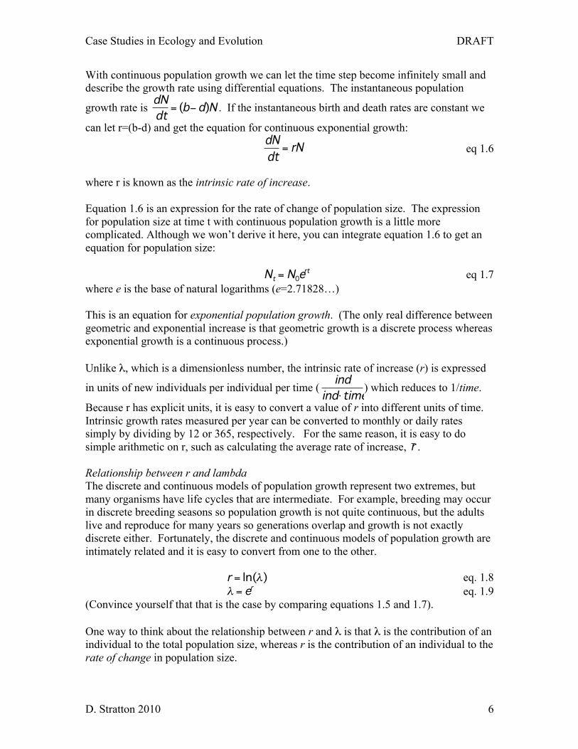
y= a+ bx). The slope of that line is r. So one way to estimate the intrinsic rate of increase is to fit a straight line to the graph of ln(N) vs time. An example is shown in figure 1.5.

Year N ln(N)

€

λ = Nt+1Nt

€

r = ln(λ) 1938 18 2.89 1.67 0.51 1948 30 3.40 1.07 0.06 1958 32 3.47 1.56 0.45 1968 50 3.91 1.50 0.41 1978 75 4.32 1.84 0.61 1988 138 4.93 1.33 0.28 1998 183 5.21 2008 270 5.60 xxxxx xxxxx

€

r = 0.39


D. Stratton 2010 9

Figure 1.5 When populations grow exponentially the logarithm of population size increases linearly with time.

Compare figure 1.5 with Figure 1.2. Notice that the relationship between ln(N)and time is approximately linear. For this population of cranes, the slope of the line is r=0.0391 per year.

How does that estimate of r compare to your estimate of

€

r from Table 1.1? __________

1.6 Forecasting future growth We’ve spent a lot of time deriving the exponential population growth model for Whooping Cranes. Why? One purpose of such a model is to forecast the future growth of the population. If the population continues growing along its current trajectory, how long will it take to reach the sustainable size of 1000 cranes? Notice that we said “if the population continues along its current trajectory”. If we are willing to assume that parameters are constant we can use this model to forecast the population size. But if conditions change then all bets are off!

Starting with the 2008 population of 270 cranes and our estimate of the intrinsic growth rate, r=0.039, what will be the population size after 10 years? __________

What will be the population size after 30 years? __________

Can you derive exact time when this population is expected to reach 1000?

y = 0.0391x - 73.041

2.00

2.50

3.00

3.50

4.00

4.50

5.00

5.50

6.00

1920 1940 1960 1980 2000 2020

Ln N

um

ber

of

Cra

nes

Year

Whooping Crane Population 1938-2008


D. Stratton 2010 10

1.7 OPTIONAL: Variation in growth rate among years Look closely at Figure 1.2 and you'll see that the population has not increased steadily every year. In some years the population increased slightly faster than average. In other years the population actually declined slightly. Many factors can influence the rate of population growth. One of the most common sources is random variation in environmental conditions. Some winters are colder than others which lead to higher than average death rates. Some breeding seasons may be particularly productive so there is a higher than average rate of reproduction. If you examine the crane population data in Appendix 1A, you will see that the average population growth rate is approximately

€

r = 0.039, corresponding to our predicted population growth curve in Figure 1.2. But in some years the estimated value of r is much higher and in others it is negative.

Figure 1.6. Year to year variation in the growth rate of the Aransas/Wood Buffalo population of whooping cranes (from Appendix 1A). When there is environmental variation in the population growth rate there can be considerable uncertainty in projecting the future popuation size. As an example, let’s consider a simple simulation. We’ll start with the same population of 18 cranes in 1938 as in Appendix 1A. Then, each year we’ll randomly choose a value of r from the observed distribution and simulate the population to the year 2000. That whole process is repeated several times. The results are shown in Figure 1.7. Averaging over all simulations, we still expect the population to grow at a rate of r=0.037. But there is considerable variation in each realization of the process. By chance, some simulations end up with larger numbers and others with smaller numbers of cranes. Figure 1.7 Ten random simulations of population growth based on the observed variation in growth rate for whooping cranes.

0

5

10

15

20

25

-0.50 -0.40 -0.30 -0.20 -0.10 0.00 0.10 0.20 0.30

Frequency

GrowthRate(r)


D. Stratton 2010 11

Why is that graph so different from Fig 1.2? Think back on the assumptions of our model. One of our assumptions was that the intrinsic growth rate, r, is a constant. If instead there is variation in r then there will be some uncertainty in the future growth of the population. Our uncertainty about the population size will increase the farther we try to project the population into the future. Figure 1.8. Prediction error increases as we forecast future growth

10 Simulations (rbar=0.0387,

0

100

200

300

400

500

600

1930 1950 1970 1990 2010

Year

N

0

500

1000

1500

2000

0 10 20 30 40 50

Num

berofCranes

YearsintheFuture


D. Stratton 2010 12

Demographic stochasticity Another source of variation in population size is known as “demographic stochasticity”. Demographic stochasticity results from the fact that population growth can never be truly continuous. Individuals come in discrete units so the population size must always be an integer (i.e. you can’t have a population size of 1.3 individuals). And even though the birth and death rates are usually fractional numbers (e.g. the probability of death may be d=0.2), each individual will die completely or not at all. So over time the population size may deviate from the predicted values based on simple exponential growth. Imagine a very small population of only a single individual. In each time period that individual can either produce one new offspring with probability 0.5 or die, again with probability of 0.5. Because the probability of births and deaths is equal, we expect the population size to remain constant. But the order of those events is important: if by chance the first event is a death, that tiny population will go extinct! As the population gets larger, the role of this demographic stochasticity is reduced. For a population of 10 individuals there is still a chance that that population will go extinct before reproduction, but only if all 10 die before they reproduce, an unlikely occurrence. Demographic stochasticity need not produce extinction. In that population of 10 individuals with b=d=0.5, we expect 5 births and 5 deaths. But it is not unlikely to have 6 births and only 4 deaths, leading to a new population of 12 individuals after one time step. In very large populations the actual number of births and deaths will be close to the expected number and demographic stochasticity becomes negligible.

1.8 Further Reading Canadian Wildlife Service and U.S. Fish and Wildlife Service. 2007. International recovery plan for the whooping crane. Ottawa: Recovery of Nationally Endangered Wildlife (RENEW), and U.S. Fish and Wildlife Service, Albuquerque, New Mexico. 162 pp. Gotelli, N.J. 2008. A Primer of Ecology, 4th edition. Sinauer


D. Stratton 2010 13

1.9 Your turn: One common example of exponential growth is in the initial spread of a disease during a new outbreak. Disease spread can be modeled in much the same way as population growth, where N is the number of infected individuals, “births” are new infections and “deaths” are the loss of infected individuals, by recovery from disease or sometimes by death. Once some individuals develop immunity to the disease the dynamics become more complicated. But the initial spread can be modeled as simple exponential growth. Here are some data from the initial spread of the 2009 outbreak of H1N1 influenza in the UK.

Graph the number of cases by week over the first four weeks of the disease. What was the growth rate of the influenza infections? (per week? per day?) What is the doubling time (in days) for the number of influenza cases during this phase of the outbreak?

Initial spread of H1N1 Swine flu in the UK, May 26 to July 1, 2009

Week Date Confirmed cases Ln Cases 0 26-May-2009 185 5.22 1 3-Jun-2009 381 5.94 2 10-Jun-2009 750 6.62 3 24-Jun-2009 3254 8.09 4 1-Jul-2009 6929 8.84


D. Stratton 2010 14

Appendix 1A. Number of Whooping Cranes in the wild Aransas/Wood Buffalo population, 1938-2007 .

Year N Ln(N) λ 1938 18 2.89 1.22 0.20 1939 22 3.09 1.18 0.17 1940 26 3.26 0.62 -0.49 1941 16 2.77 1.19 0.17 1942 19 2.94 1.11 0.10 1943 21 3.04 0.86 -0.15 1944 18 2.89 1.22 0.20 1945 22 3.09 1.14 0.13 1946 25 3.22 1.24 0.22 1947 31 3.43 0.97 -0.03 1948 30 3.40 1.13 0.13 1949 34 3.53 0.91 -0.09 1950 31 3.43 0.81 -0.22 1951 25 3.22 0.84 -0.17 1952 21 3.04 1.14 0.13 1953 24 3.18 0.88 -0.13 1954 21 3.04 1.33 0.29 1955 28 3.33 0.86 -0.15 1956 24 3.18 1.08 0.08 1957 26 3.26 1.23 0.21 1958 32 3.47 1.03 0.03 1959 33 3.50 1.09 0.09 1960 36 3.58 1.08 0.08 1961 39 3.66 0.82 -0.20 1962 32 3.47 1.03 0.03 1963 33 3.50 1.27 0.24 1964 42 3.74 1.05 0.05 1965 44 3.78 0.98 -0.02 1966 43 3.76 1.12 0.11 1967 48 3.87 1.04 0.04 1968 50 3.91 1.12 0.11 1969 56 4.03 1.02 0.02 1970 57 4.04 1.04 0.03 1971 59 4.08 0.86 -0.15 1972 51 3.93 0.96 -0.04 1973 49 3.89 1.00 0.00 1974 49 3.89 1.16 0.15 1975 57 4.04 1.21 0.19 1976 69 4.23 1.04 0.04 1977 72 4.28 1.04 0.04 1978 75 4.32 1.01 0.01

1979 76 4.33 1.03 0.03 1980 78 4.36 0.94 -0.07 1981 73 4.29 1.00 0.00 1982 73 4.29 1.03 0.03 1983 75 4.32 1.16 0.15 1984 87 4.47 1.11 0.11 1985 97 4.57 1.13 0.13 1986 110 4.70 1.22 0.20 1987 134 4.90 1.03 0.03 1988 138 4.93 1.06 0.06 1989 146 4.98 1.00 0.00 1990 146 4.98 0.90 -0.10 1991 132 4.88 1.03 0.03 1992 136 4.91 1.05 0.05 1993 143 4.96 0.93 -0.07 1994 133 4.89 1.19 0.17 1995 158 5.06 1.01 0.01 1996 160 5.08 1.14 0.13 1997 182 5.20 1.01 0.01 1998 183 5.21 1.03 0.03 1999 188 5.24 0.96 -0.04 2000 180 5.19 0.97 -0.03 2001 175 5.16 1.06 0.06 2002 185 5.22 1.05 0.05 2003 194 5.27 1.12 0.11 2004 217 5.38 1.01 0.01 2005 220 5.39 1.08 0.07 2006 237 5.47 1.12 0.11 2007 266 5.58

€

r = ln(λ )


D. Stratton 2010 15

1 Population growth: The return of the Whooping Crane

Documents

Transcript of 1 Population growth: The return of the Whooping Crane