
Pointwise Extensions of GSOS-De ned Operations - TU...
39
Under consideration for publication in Math. Struct. in Comp. Science Pointwise Extensions of GSOS-Defined Operations HELLE HVID HANSEN 1 and BARTEK KLIN 2† 1 Technische Universiteit Eindhoven and Centrum Wiskunde & Informatica, P.O.Box 513, 5300 MB Eindhoven, The Netherlands. Email: [email protected]. 2 University of Cambridge and University of Warsaw, 15 JJ Thomson Avenue, Cambridge CB3 0FD, UK. Email: [email protected]. Received 3 February 2011 Final coalgebras capture system behaviours such as streams, infinite trees and processes. Algebraic operations on a final coalgebra can be defined by distributive laws (of a syntax functor Σ over a behaviour functor F ). Such distributive laws correspond to abstract specification formats. One such format is a generalisation of the GSOS rules known from structural operational semantics of processes. We show that given an abstract GSOS specification ρ that defines operations σ on a final F -coalgebra, we can systematically construct a GSOS specification ρ that defines the pointwise extension σ of σ on a final F A -coalgebra. The construction relies on adding a family of auxiliary “buffer” operations to the syntax. These buffer operations depend only on A, and so the construction is uniform for all σ and F . 1. Introduction In coalgebra, state-based systems are modelled as F -coalgebras where F is a functor that determines the system type. By varying F , we obtain (non)deterministic automata, (labelled) transition systems and many others, see (Rutten 2000) for an introduction and plenty of examples. Of particular importance are final coalgebras, which represent abstract behaviours of F -coalgebras. For this reason we refer to elements of a final F - coalgebra as F -behaviours. Examples of F -behaviours include streams, infinite trees, causal stream functions and processes. Thanks to the properties of final coalgebras, op- erations on them can be conveniently defined by coinduction. In this paper, we focus on pointwise extensions of operations on F -behaviours to opera- tions on F A -behaviours, where F is an arbitrary functor, and A is a fixed set. Intuitively, F A -coalgebras behave as F -coalgebras, but are additionally dependent on an external source of input from the alphabet A. For example, if FX = B ×X then F A -coalgebras are † Supported by EPSRC grant EP/F042337/1.
Transcript of Pointwise Extensions of GSOS-De ned Operations - TU...

Under consideration for publication in Math. Struct. in Comp. Science
Pointwise Extensions of GSOS-DefinedOperations
H E L L E H V I D H A N S E N1 and B A R T E K K L I N2†
1 Technische Universiteit Eindhoven and Centrum Wiskunde & Informatica,P.O.Box 513, 5300 MB Eindhoven, The Netherlands.Email: [email protected] University of Cambridge and University of Warsaw,15 JJ Thomson Avenue, Cambridge CB3 0FD, UK.Email: [email protected].
Received 3 February 2011
Final coalgebras capture system behaviours such as streams, infinite trees and processes.
Algebraic operations on a final coalgebra can be defined by distributive laws (of a syntax
functor Σ over a behaviour functor F ). Such distributive laws correspond to abstract
specification formats. One such format is a generalisation of the GSOS rules known from
structural operational semantics of processes. We show that given an abstract GSOS
specification ρ that defines operations σ on a final F -coalgebra, we can systematically
construct a GSOS specification ρ that defines the pointwise extension σ of σ on a final
FA-coalgebra. The construction relies on adding a family of auxiliary “buffer” operations
to the syntax. These buffer operations depend only on A, and so the construction is
uniform for all σ and F .
1. Introduction
In coalgebra, state-based systems are modelled as F -coalgebras where F is a functorthat determines the system type. By varying F , we obtain (non)deterministic automata,(labelled) transition systems and many others, see (Rutten 2000) for an introductionand plenty of examples. Of particular importance are final coalgebras, which representabstract behaviours of F -coalgebras. For this reason we refer to elements of a final F -coalgebra as F -behaviours. Examples of F -behaviours include streams, infinite trees,causal stream functions and processes. Thanks to the properties of final coalgebras, op-erations on them can be conveniently defined by coinduction.
In this paper, we focus on pointwise extensions of operations on F -behaviours to opera-tions on FA-behaviours, where F is an arbitrary functor, and A is a fixed set. Intuitively,FA-coalgebras behave as F -coalgebras, but are additionally dependent on an externalsource of input from the alphabet A. For example, if FX = B×X then FA-coalgebras are
† Supported by EPSRC grant EP/F042337/1.
H.H. Hansen and B. Klin 2
Mealy machines with input in A and output in B, and FA-behaviours are causal streamfunctions f : Aω → Bω. We show that, in general, elements of the set Z of FA-behaviourscan be thought of as certain functions from Aω to a final F -coalgebra Z. An operation σon Z can therefore be pointwise extended in the standard way to an operation σ on thefunction space ZA
ω
. Depending on σ, the operation σ restricts or not to an operation onZ.
A well-structured way of defining operations on final coalgebras is by means of dis-tributive laws of syntax over behaviour (cf. Turi and Plotkin 1997; Bartels 2004; Klin2009), where syntax is given by an algebraic signature Σ and behaviour is given by afunctor F . The rather abstract notion of a distributive law can often be formulated ina more intuitive fashion as a set of equations or rules. Concrete examples include Rut-ten’s behavioural differential equations (see e.g. Rutten 2003) and rules of structuraloperational semantics of processes (cf. Aceto et al. 2001).
Distributive laws provide a setting in which specification formats for varying syntaxand behaviour types can be treated in a uniform way (using parametricity in Σ andF ). In particular, the GSOS format of processes (cf. Aceto et al. 2001) generalises to anabstract GSOS format for arbitrary Σ and F . A further benefit of working in this moreabstract setting is that a distributive law of Σ over F not only defines Σ-operations onF -behaviours, but also provides an inductive definition of an F -coalgebra on Σ-terms,and relates the final semantics of the latter with the initial semantics of the former.
Viewing specification formats as distributive laws, it makes sense to ask the following:given an operation σ, defined on a final F -coalgebra by a distributive law λ, is its point-wise extension σ an operation on a final FA-coalgebra defined by another distributive lawλ, and can we obtain λ from λ in a systematic manner? The main technical contributionof this paper is an affirmative answer to that question under certain conditions. In Theo-rem 6.1, we show that definitions in a simple format can be extended in a straightforwardmanner. Then, in Theorem 6.3, we deal with the more expressive, abstract GSOS for-mat, where the situation is more subtle. We show that GSOS-defined operations can alsobe extended pointwise, but the extension relies on a family of auxiliary operations thatintuitively work as “input buffers” for FA-coalgebras. It is worth noting that the choiceof auxiliary operators depends only on the set A, but does not depend on λ, nor even onthe behaviour functor F . In order to illustrate these general results, we provide severaldetailed examples. We mention that an extended abstract of this paper has appeared as(Hansen and Klin 2010).
The structure of the paper is as follows. In Section 2, basic facts on Set-functors,algebras and coalgebras are recalled, together with a few examples of F -coalgebras thatare used in the paper. Section 3 contains two simple examples of operations on streams,and their pointwise extensions to Mealy machines. The techniques used in these examplesmotivate, and hopefully provide some intuition about, the abstract development of thesubsequent sections. In Section 4 we show how to interpret elements of FA-coalgebras asfunctions from A-streams to final F -coalgebras via their pointwise behaviour; based onthis, we provide an abstract definition of pointwise extension of operations, illustrated bya few examples. In Section 5 we recall the distributive law approach to defining operations,as developed in (Turi and Plotkin 1997; Lenisa et al. 2004). Section 6 contains the two

Pointwise Extensions of GSOS-Defined Operations 3
main technical theorems as described above, followed by a few example applications inSection 7, and a brief discussion of directions for future work in Section 8. Proofs of themain theorems are put in an Appendix.
2. Preliminaries
In this section we fix some notation and provide the basic definitions of algebras andcoalgebras needed in this paper. We assume that the reader is familiar with the notionsof category, functor, natural transformation; the notions of adjunction and monad arementioned a few times, but their detailed understanding is not necessary to follow themain development. All functors considered in this paper are endofunctors on Set, thecategory of sets and functions.
2.1. Strength and costrength
We recall some basic properties of Set functors that will be useful in the following.For any set A, there is an adjunction A×− a (−)A. The obvious unit and the counit
of this adjunction will be denoted
ηX : X → (A×X)A εX : A×XA → X.
Any endofunctor F on Set has a strength, i.e., a map
stFA,X : A× FX → F (A×X)
natural in A and X, defined by
stFA,X(a, t) = (Fηa)(t)
where ηa : X → A×X is given by ηa(x) = (a, x). Dually, every F has a costrength
csFA,X : F (XA)→ (FX)A
natural in A and X, defined by
csFA,X(t)(a) = (Fεa)(t)
where εa : XA → X is given by εa(f) = f(a).
2.2. Syntax via algebras
An algebraic signature Σ consists of a collection of function symbols {σi | i ∈ I} whereeach σi has an arity ni ∈ N, i ∈ I. A Σ-algebra with carrier set X is a map
∐i∈I X
ni → X
and we therefore identify a signature Σ with the functor ΣX =∐i∈I X
ni . In general,given a functor G , a G-algebra is a pair 〈X,σ〉 where X is the carrier set and σ : GX → X
is a function.The set of Σ-terms over a set (of variables) X is denoted by TΣX; we shall omit the
subscript in the following, as it will never lead to any confusion. In fact, T is a functor, andtogether with obvious natural transformations ηT : Id =⇒ T (interpretation of variables
H.H. Hansen and B. Klin 4
as terms) and µT : TT =⇒ T (glueing terms built of terms) it forms the so-called freemonad over Σ. By structural induction on terms, any algebra σ : ΣX → X induces afunction σ] : TX → X (i.e. term interpretation in σ). The T -algebra σ] satisfies axioms:
σ] ◦ ηTX = idX σ] ◦ Tσ] = σ] ◦ µTX ,
i.e., σ] is an Eilenberg-Moore algebra for the monad T . The construction of σ] from σ
provides a 1-1 correspondence between Σ-algebras and Eilenberg-Moore T -algebras.
2.3. Behaviour via coalgebras
Coalgebra provides a uniform framework for studying the behaviour of systems such asautomata and labelled transition systems. We only provide the basic definitions here.For a more thorough introduction to the theory of coalgebra we refer to (Rutten 2000).Formally, given a functor F , an F -coalgebra is a pair 〈X, ξ〉 where X is a set (called thecarrier, or the set of states) and ξ : X → FX is a function (called the structure). Sinceξ : X → FX implicitly defines the carrier X, we often refer to an F -coalgebra simplyby its structure. Different types of systems emerge by varying F . We provide concreteexamples in Section 2.4.
Behaviour preserving maps are formalised as the general notion of morphism betweenF -coalgebras. An F -coalgebra morphism h : 〈X1, ξ1〉 → 〈X2, ξ2〉 is a function h : X1 →X2 such that ξ2 ◦h = Fh ◦ ξ1. F -coalgebras and F -coalgebra morphisms form a categoryCoalg(F ). An abstract notion of behaviour is obtained via finality. An F -coalgebra 〈Z, ζ〉is final, if for every F -coalgebra 〈X, ξ〉 there is a unique F -coalgebra morphism beh〈X,ξ〉(called the final map) from 〈X, ξ〉 to 〈Z, ζ〉. A final F -coalgebra 〈Z, ζ〉 can be seen asa system of behaviours, and we refer to the elements of Z as F -behaviours. By the so-called Lambek lemma (Lambek 1968), the structure ζ of a final coalgebra is always anisomorphism. A final F -coalgebra need not always exist due to cardinality reasons, (cf.Aczel and Mendler 1989), but all functors considered in this paper admit final coalgebras.
The existence and uniqueness of the final map give rise to a definition principle usuallyreferred to as coinduction. We will use coinduction to define operations on the carriersof final coalgebras. Let F be a functor and 〈Z, ζ〉 the final F -coalgebra. By defining anF -coalgebra structure ξ : Z × Z → F (Z × Z) the final map behξ : Z × Z → Z definesa binary operation ? on Z by coinduction. So the F -coalgebra structure ξ essentiallyspecifies how x ? y behaves for all x, y ∈ Z. More generally, for an algebraic signature Σ,an F -coalgebra structure on ΣZ induces a Σ-algebra on Z by coinduction as illustratedhere:
ΣZ
ξ
��
σ // Z
ζ
��
FΣZFσ // FZ
(1)
In Section 5 we will see how certain natural transformations correspond to various kindsof the specification ξ.

Pointwise Extensions of GSOS-Defined Operations 5
2.4. Examples
We shall now see a number of concrete examples of functors and their final coalgebras.All of these are well known, but we include them in some detail as they will be used lateron for illustrating pointwise extensions.
Example 2.1 (Stream automata) Given a set A, a stream automaton (with output inA) is a coalgebra for the functor A × −, i.e., it is a function 〈o, d〉 : X → A ×X whichmaps an x ∈ X to an output value o(x) ∈ A and a next state d(x) ∈ X. We will usethe notation x a→ y to denote that o(x) = a and d(x) = y. The final (A×−)-coalgebrais obtained as the set Aω of streams over A together with the head and tail maps,〈hd , tl〉 : Aω → A × Aω. The (A × −)-behaviour of a state x is the stream of outputsgenerated on transitions starting in x. We will use the following standard notation. Astream α ∈ Aω may be written (α(0), α(1), α(2), . . .) or as an ω-regular expression overA. For α ∈ Aω and n ∈ N, α�n= (α(0), . . . , α(n)) is the prefix of α of length n + 1. Forα ∈ Aω and a ∈ A, we denote with a :α the stream (a, α(0), α(1), . . .). �
Example 2.2 (Mealy machines) Given sets A and B, a (B×−)A-coalgebra m : X →(B ×X)A is a Mealy machine with input in A and output in B: for each state x ∈ X,m(x) = 〈ox, dx〉 : A→ B×X defines for each a ∈ A, the output ox(a) and the next state
dx(a). We write x a|b→ y if ox(a) = b and dx(a) = y. The behaviour of a state x is theinput-output mapping computed by m : X → (B × X)A when starting in x. Formally,beh(x) : Aω → Bω maps α ∈ Aω to the stream beh(x)(α) ∈ Bω where for all n ∈ N:
beh(x)(α)(n) = oxn(α(n)) x0 := x, xn+1 := dxn
(α(n)). (2)
From (2) it is clear that the n-th element of beh(x)(α) depends only on α(0), . . . , α(n).A stream function f : Aω → Bω is causal if for all n ∈ N, and all α, β ∈ Aω:
α�n = β�n =⇒ f(α)(n) = f(β)(n).
The set Γ = {f : Aω → Bω | f is causal } carries a final Mealy structure as shown in(Rutten 2006). We briefly summarise the construction. Let f ∈ Γ and a ∈ A. We writef(a :−) for the stream function which maps α ∈ Aω to f(a :α) ∈ Bω. The initial outputf [a] and the stream function derivative fa of f on a are defined as:
f [a] := hd ◦ f(a :−) ∈ Aω → B
fa := tl ◦ f(a :−) ∈ Aω → Bω(3)
Since f is causal, f [a] is constant (so we can consider f [a] an element of B) and fa iscausal, hence by defining for all f ∈ Γ and a ∈ A,
γ(f)(a) = 〈f [a], fa〉,
γ is a map of type γ : Γ → (B × Γ)A, and it can be shown that 〈Γ, γ〉 is a final Mealymachine. �
Example 2.3 (Partial maps) We denote the one-element set by 1 = {⊥}. If we let ⊥represent the undefined value, then a (1 + −)-coalgebra ξ : X → 1 + X can be seen as
H.H. Hansen and B. Klin 6
a partial function on X, and we write x → y if ξ(x) = y (for y ∈ 1 + X). The final(1 + −)-coalgebra consists of the natural numbers extended with ω together with thepredecessor function pred : N + {ω} → 1 + N + {ω} where pred(0) = ⊥, pred(ω) = ω
and pred(n) = n− 1 for all n ∈ N>0. The behaviour of a state x is the number of stepsthat can be made from x. �
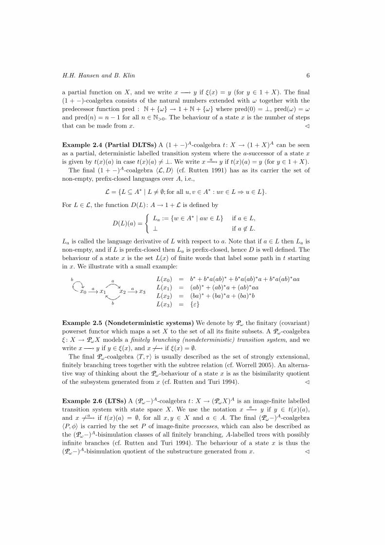
Example 2.4 (Partial DLTSs) A (1 + −)A-coalgebra t : X → (1 + X)A can be seenas a partial, deterministic labelled transition system where the a-successor of a state xis given by t(x)(a) in case t(x)(a) 6= ⊥. We write x a→ y if t(x)(a) = y (for y ∈ 1 +X).
The final (1 + −)A-coalgebra 〈L, D〉 (cf. Rutten 1991) has as its carrier the set ofnon-empty, prefix-closed languages over A, i.e.,
L = {L ⊆ A∗ | L 6= ∅; for all u, v ∈ A∗ : uv ∈ L⇒ u ∈ L}.
For L ∈ L, the function D(L) : A→ 1 + L is defined by
D(L)(a) =
{La := {w ∈ A∗ | aw ∈ L} if a ∈ L,⊥ if a 6∈ L.
La is called the language derivative of L with respect to a. Note that if a ∈ L then La isnon-empty, and if L is prefix-closed then La is prefix-closed, hence D is well defined. Thebehaviour of a state x is the set L(x) of finite words that label some path in t startingin x. We illustrate with a small example:
x0a //
b
��x1
a
��x2
b
]]
a // x3
L(x0) = b∗ + b∗a(ab)∗ + b∗a(ab)∗a+ b∗a(ab)∗aaL(x1) = (ab)∗ + (ab)∗a+ (ab)∗aaL(x2) = (ba)∗ + (ba)∗a+ (ba)∗bL(x3) = {ε}
Example 2.5 (Nondeterministic systems) We denote by Pω the finitary (covariant)powerset functor which maps a set X to the set of all its finite subsets. A Pω-coalgebraξ : X → PωX models a finitely branching (nondeterministic) transition system, and wewrite x → y if y ∈ ξ(x), and x 6 → if ξ(x) = ∅.
The final Pω-coalgebra 〈T, τ〉 is usually described as the set of strongly extensional,finitely branching trees together with the subtree relation (cf. Worrell 2005). An alterna-tive way of thinking about the Pω-behaviour of a state x is as the bisimilarity quotientof the subsystem generated from x (cf. Rutten and Turi 1994). �
Example 2.6 (LTSs) A (Pω−)A-coalgebra t : X → (PωX)A is an image-finite labelledtransition system with state space X. We use the notation x a→ y if y ∈ t(x)(a),and x 6 a→ if t(x)(a) = ∅, for all x, y ∈ X and a ∈ A. The final (Pω−)A-coalgebra〈P, φ〉 is carried by the set P of image-finite processes, which can also be described asthe (Pω−)A-bisimulation classes of all finitely branching, A-labelled trees with possiblyinfinite branches (cf. Rutten and Turi 1994). The behaviour of a state x is thus the(Pω−)A-bisimulation quotient of the substructure generated from x. �
Pointwise Extensions of GSOS-Defined Operations 7
3. Motivating Examples
To motivate the abstract development of Sections 4 and 6, and provide some intuitionsabout the techniques used there, we shall begin with two concrete examples of operationson the set Rω of streams over the real numbers, i.e. the carrier of a final (R×−)-coalgebra,and show how to extend their definitions to operations on causal stream functions.
As explained in (Rutten 2003), operations on streams can be defined with the help ofstream differential equations, where the resulting stream is unambiguously specified byits initial value (head) and its stream derivative (tail) in terms of the initial values andthe derivatives of the argument streams.
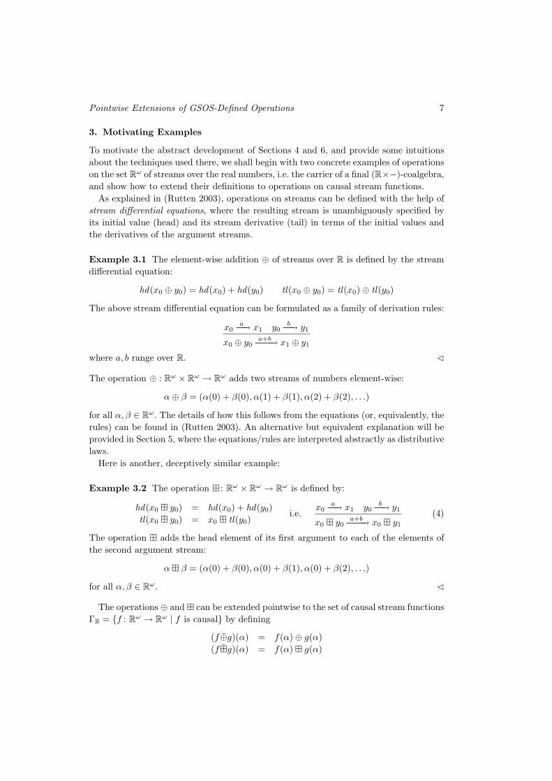
Example 3.1 The element-wise addition ⊕ of streams over R is defined by the streamdifferential equation:
hd(x0 ⊕ y0) = hd(x0) + hd(y0) tl(x0 ⊕ y0) = tl(x0)⊕ tl(y0)
The above stream differential equation can be formulated as a family of derivation rules:
x0a→ x1 y0
b→ y1
x0 ⊕ y0a+b→ x1 ⊕ y1
where a, b range over R. �
The operation ⊕ : Rω × Rω → Rω adds two streams of numbers element-wise:
α⊕ β = (α(0) + β(0), α(1) + β(1), α(2) + β(2), . . .)
for all α, β ∈ Rω. The details of how this follows from the equations (or, equivalently, therules) can be found in (Rutten 2003). An alternative but equivalent explanation will beprovided in Section 5, where the equations/rules are interpreted abstractly as distributivelaws.
Here is another, deceptively similar example:
Example 3.2 The operation � : Rω × Rω → Rω is defined by:
hd(x0 � y0) = hd(x0) + hd(y0)tl(x0 � y0) = x0 � tl(y0)
i.e.x0
a→ x1 y0b→ y1
x0 � y0a+b→ x0 � y1
(4)
The operation � adds the head element of its first argument to each of the elements ofthe second argument stream:
α� β = (α(0) + β(0), α(0) + β(1), α(0) + β(2), . . .)
for all α, β ∈ Rω. �
The operations ⊕ and � can be extended pointwise to the set of causal stream functionsΓR = {f : Rω → Rω | f is causal} by defining
(f⊕g)(α) = f(α)⊕ g(α)(f�g)(α) = f(α) � g(α)

H.H. Hansen and B. Klin 8
for all f, g ∈ ΓR and α ∈ Rω. Note in particular, that f⊕g and f�g are again causal,so ⊕ and � are well defined as operations on ΓR. In general, given an n-ary operationσ on a set Y , the pointwise extension of σ to the function space Y X , is the operationσ : (Y X)n → Y X defined for all f0, . . . , fn−1 : X → Y by
σ(f0, . . . , fn−1)(x) = σ(f0(x), . . . , fn−1(x)).
The question is, can we give a rule-based definition of the pointwise extensions ⊕ and �,possibly based on the defining rules for ⊕ and �, respectively?
Recall from Example 2.2 that ΓR is the final (R×−)R-coalgebra under the operations
initial output f [a] and stream function derivative fa. Using the notation fa|f [a]→ fa,
the pointwise extension ⊕ : ΓR × ΓR → ΓR can be defined as follows:
x0a|b→ x1 y0
a|c→ y1
x0⊕y0a|b+c→ x1⊕y1
(5)
To see how this rule works, suppose that α = (a0, a1, a2, . . .) ∈ Rω and f, g ∈ ΓR withf(α) = (b0, b1, b2, . . .) and g(α) = (c0, c1, c2, . . .). It follows, in particular, that for therepeated derivatives we have: fa0...an [an+1] = bn+1 and ga0...an [an+1] = cn+1 for alln ∈ N. The rule in (5) induces the following transitions of f⊕g on input α:
f⊕g a0|b0+c0→ fa0⊕ga0
a1|b1+c1→ fa0a1⊕ga0a1
a2|b2+c2→ . . .
and we see that (f⊕g)(α) = f(α)⊕g(α). Since α was arbitrary, ⊕ is indeed the pointwiseextension of ⊕.
Let us now consider the pointwise extension of �. By analogy with (5), we could tryto define � : ΓR × ΓR → ΓR with the following rule:
x0a|b→ x1 y0
a|c→ y1
x0�y0a|b+c→ x0�y1
(6)
For f, g ∈ ΓR, the rule (6) implies that for all a ∈ R:
(f�g)[a] = f [a] + g[a](f�g)a = f�ga
(7)
However, the induced operation on ΓR is not the pointwise extension of �. To see this,consider id�id where id is the identity on Rω. Note that in particular, id[a] = a andida = id for all a ∈ R. The rule (6) then yields the following transitions on inputα = (a0, a1, a2, . . .) ∈ Rω:
id�id a0|a0+a0→ id�id a1|a1+a1→ id�id a2|a2+a2→ . . .
hence (id�id)(α) 6= α� α = (a0 + a0, a0 + a1, a0 + a2, . . .).To understand what goes wrong, we must look into the structure of the final Mealy
machine. Recall from Example 2.2 that for all f ∈ ΓR and a ∈ R, fa = tl(f(a :−)). Inorder for � to be the pointwise extension of �, the following must hold for all f, g ∈ ΓR,a ∈ R and α ∈ Rω:
(f�g)(a :α) = f(a :α) � g(a :α).

Pointwise Extensions of GSOS-Defined Operations 9
By taking tails on both sides, and applying the rule (4) for � we get
(f�g)a(α) = f(a :α) � ga(α). (8)
Comparing (8) with (7), we see that in the definition of (f�g)a, f should be replacedwith the function f(a :−). In order to give a rule-based definition of � (which appliesnot only to ΓR, but to all Mealy machines), it makes sense to use a family of auxiliary,unary operations {a .− | a ∈ R}. These operations act like one-element input buffers:for a Mealy machine m : X → (R×X)R and x ∈ X, a . x behaves like x as if it had seenan a already. Formally, beh(a . x)(α) = beh(x)(a :α) for all α ∈ Rω and a ∈ R. We cannow define �, together with the buffer operations, by rules:
x0a|b→ x1 y0
a|c→ y1
x0�y0a|b+c→ (a . x0)�y1
x0a|b→ x1
a . x0c|b→ c . x1
(9)
To illustrate how this definition works, let α = (a0, a1, a2, . . .) ∈ Rω and f, g ∈ ΓR withf(α) = (b0, b1, b2, . . .) and g(α) = (c0, c1, c2, . . .). First, the rule for a .− gives us,
fa0|b0→ fa0 =⇒ (a0 . f) a1|b0→ (a1 . fa0)
=⇒ (a1 . a0 . f) a2|b0→ (a2 . a1 . fa0)
=⇒ (a2 . a1 . a0 . f) a3|b0→ (a3 . a2 . a1 . fa0)
=⇒ . . .
We now find that,
f�ga0|b0+c0→ (a0 . f)�ga0
a1|b0+c1→ (a1 . a0 . f)�ga0a1
a2|b0+c2→ (a2 . a1 . a0 . f)�ga0a1a2
a3|b0+c3→ . . .
So � indeed behaves as the pointwise extension of �.In the rest of this paper, we show that the constructions used in the above examples
apply more generally. In particular, the idea of defining pointwise extensions by addinginput buffer operations works not only for the specific stream operation �, but in factfor all GSOS-defined operations on F -behaviours, for any functor F . The meaning of thephrase “GSOS-defined” is explained in detail in Section 5. Before that, however, we needto understand the notion of pointwise extension for operations on final F -coalgebras.
4. Pointwise Behaviour and Pointwise Extensions of Operations
In this section, we introduce the notion of pointwise behaviour of F -coalgebras withinput. From now on, let A be a fixed set. An F -coalgebra with input (in A) is a coalgebrafor the functor composition FA = (−)A ◦F . That is, FA(X) = (FX)A and for a functionf : X → Y , FA(f) : (FX)A → (FY )A is defined by FA(f)(t)(a) = (Ff)(t(a)). Ourmotivating examples in Section 3 focused on the case where F = (B × −), that is, FA-coalgebras are Mealy machines, and FA-behaviours are causal stream functions of type
H.H. Hansen and B. Klin 10
f : Aω → Bω. Evaluating such a causal stream function at an input stream α ∈ Aω
yields an element in Bω, the set of F -behaviours. We will show that for any functorF , under the assumption that the final coalgebras for F and FA exist, we can evaluateFA-behaviours at input streams from Aω to obtain F -behaviours. This observation relieson a construction which is similar to the wreath product of automata (cf. Carton 2000;Straubing 1989).
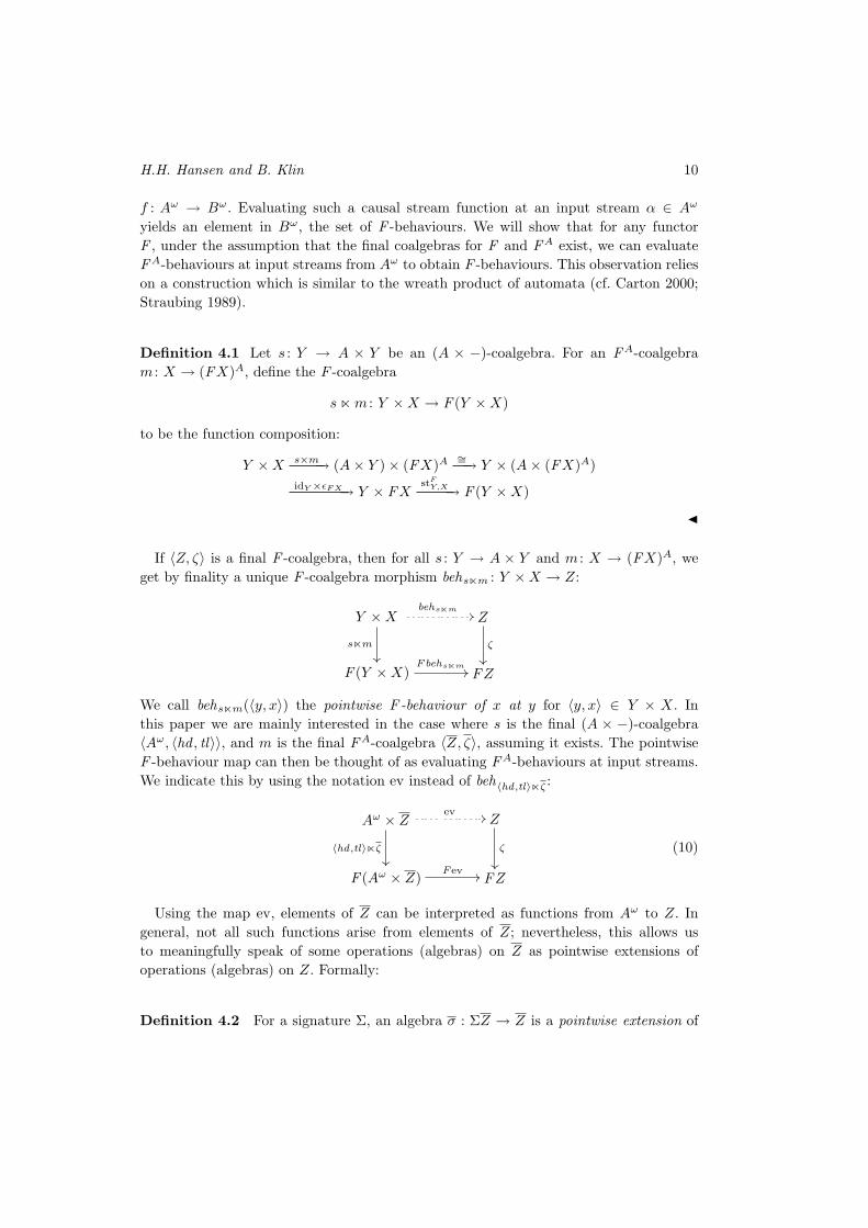
Definition 4.1 Let s : Y → A × Y be an (A × −)-coalgebra. For an FA-coalgebram : X → (FX)A, define the F -coalgebra
snm : Y ×X → F (Y ×X)
to be the function composition:
Y ×X s×m→ (A× Y )× (FX)A∼=→ Y × (A× (FX)A)
idY ×εF X→ Y × FXstFY,X→ F (Y ×X)
�
If 〈Z, ζ〉 is a final F -coalgebra, then for all s : Y → A × Y and m : X → (FX)A, weget by finality a unique F -coalgebra morphism behsnm : Y ×X → Z:
Y ×X
snm��
behsnm// Z
ζ
��
F (Y ×X)Fbehsnm
// FZ
We call behsnm(〈y, x〉) the pointwise F -behaviour of x at y for 〈y, x〉 ∈ Y × X. Inthis paper we are mainly interested in the case where s is the final (A × −)-coalgebra〈Aω, 〈hd , tl〉〉, and m is the final FA-coalgebra 〈Z, ζ〉, assuming it exists. The pointwiseF -behaviour map can then be thought of as evaluating FA-behaviours at input streams.We indicate this by using the notation ev instead of beh〈hd,tl〉nζ :
Aω × Z
〈hd,tl〉nζ��
ev // Z
ζ
��
F (Aω × Z)Fev // FZ
(10)
Using the map ev, elements of Z can be interpreted as functions from Aω to Z. Ingeneral, not all such functions arise from elements of Z; nevertheless, this allows usto meaningfully speak of some operations (algebras) on Z as pointwise extensions ofoperations (algebras) on Z. Formally:
Definition 4.2 For a signature Σ, an algebra σ : ΣZ → Z is a pointwise extension of

Pointwise Extensions of GSOS-Defined Operations 11
σ : ΣZ → Z if the diagram:
Aω × ΣZ
id×σ��
stΣAω,Z
// Σ(Aω × Z)Σev // ΣZ
σ
��
Aω × Z ev// Z
(11)
commutes. �
We now show a few examples of pointwise behaviour and pointwise extensions.
Example 4.3 In our main example of streams and Mealy machines, the relevant functorsare F = (B × −) and FA = (B × −)A, F -behaviours are streams over B and FA-behaviours are causal stream functions of type f : Aω → Bω (cf. Example 2.2). Theinput evaluation and pointwise behaviour of causal stream functions are illustrated inthe diagram below. To ease notation, we write α0 and α′ for hd(α) and tl(α), respectively.
Aω × Γ
〈hd,tl〉nγ��
〈α, f〉_
��
� ev // f(α)_
��
Bω
〈hd,tl〉��
B × (Aω × Γ) 〈f [α0], 〈α′, fα0〉〉id×ev
// 〈f [α0], fα0(α′)〉 B ×Bω
Clearly, for all f ∈ Γ and α ∈ Aω, ev(〈α, f〉) = f(α).In Section 3 we have already seen examples of pointwise extensions of stream operations
to causal stream functions. We note, however, that not all stream operations can beextended pointwise to Γ. A simple example is given by the tail operation tl : Bω → Bω.Its pointwise extension tl : Γ → Γ would have to be defined for f ∈ Γ and α ∈ Aω bytl(f)(α) = tl(f(α)). But then tl(f) is not causal, in general. For example, taking A = B
and f = id, then tl(id) = tl which is not causal, so tl is not well defined as an operationon Γ.
On the other hand, causal stream operations can be pointwise extended to Γ. Moreprecisely, we say that a k-ary operation σ : (Bω)k → Bω is causal if for all β0, . . . , βk−1 ∈Bω and all n ∈ N, σ(β0, . . . , βk−1)(n) depends only on βi�n for i ∈ {0, . . . , k − 1}. It isstraightforward to show that if σ : (Bω)k → Bω is causal, then its pointwise extensionσ preserves causality, i.e., for f0, . . . , fk−1 ∈ Γ, σ(f0, . . . , fk−1) : Aω → Bω is causal, andhence σ is a well defined operation on Γ. �
Example 4.4 Consider the functor FX = 1 + X. Recall from Examples 2.3 and 2.4that the set of F -behaviours is the extended natural numbers, and the final FA-coalgebra〈L, D〉 is carried by the set of non-empty, prefix-closed languages. A transition in the F -coalgebra 〈hd , tl〉nD is defined by:
Aω × L 〈hd,tl〉nD→ 1 + (Aω × L)
〈α0 :α′, L〉 7−→{〈α′, Lα0〉 if α0 ∈ L⊥ if α0 6∈ L

H.H. Hansen and B. Klin 12
Given a state x in an FA-coalgebra t : X → (1 + X)A and an α ∈ Aω, the pointwiseF -behaviour of x on α is the number of steps that can be made in t starting from x oninput α. More precisely,
ev(〈α, x〉) = sup{n ≤ ω | α�n ∈ L(x)} ∈ N + {ω}.
In particular, if α labels an infinite path starting in x, then ev(〈α, x〉) = ω.As an example, consider the following (fragment of the final) (1 +−)A-coalgebra with
input alphabet A = {a, b}:
x1
a
!!x2
b
aa
a
ss
We list a few examples of pointwise behaviours:
ev(〈aω, x1〉) = ω, ev(〈aω, x2〉) = ω,
ev(〈bω, x1〉) = 0, ev(〈bω, x2〉) = 1,ev(〈anbω, x1〉) = n+ 1, ev(〈anbω, x2〉) = n+ 1, ∀n > 0.
Natural operations on F -behaviours are max (∨), plus (+) and times (·) in the extendedarithmetic where ω + x = ω for all x ∈ {ω}+ N and ω · x = ω for all x ∈ {ω}+ N>0 andω · 0 = 0. Using the above example, the pointwise extensions of these operations shouldsatisfy:
ev(〈aω, x1∨x2〉) = ω, ev(〈bω, x1∨x2〉) = 1,ev(〈aω, x1 ·x2〉) = ω, ev(〈bω, x1+x2〉) = 1,ev(〈aω, x1+x2〉) = ω, ev(〈bω, x1 ·x2〉) = 0,
ev(〈anbω, x1∨x2〉) = n+ 1,ev(〈anbω, x1+x2〉) = 2n+ 2,ev(〈anbω, x1 ·x2〉) = n2 + 2n+ 1, ∀n > 0.
�
Example 4.5 Recall from Examples 2.5 and 2.6 that the final Pω-coalgebra 〈T, τ〉 con-sists of all strongly extensional, finitely branching trees with the subtree relation, andthe final PA
ω -coalgebra 〈P, φ〉 is carried by the set of image-finite processes. For α ∈ Aωand p ∈ P ,
Aω × P 〈hd,tl〉nφ→ Pω(Aω × P )
〈α, p〉 7−→ {〈α′, q〉 | p α0→ q}.
Evaluating p ∈ P at an input stream α ∈ Aω can be seen as removing from p the pathsthat are not labelled by a prefix of α, and dropping labels. The pointwise behaviour isobtained by quotienting the resulting tree with Pω-bisimilarity. For example, let A =
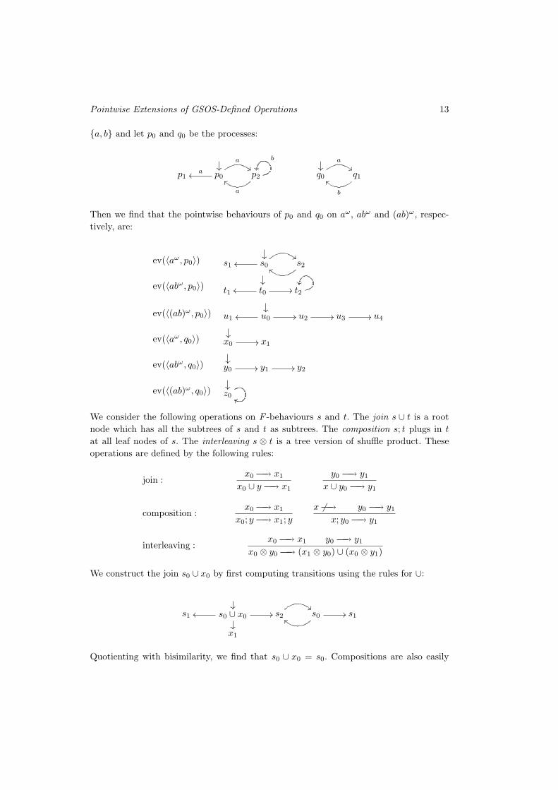
Pointwise Extensions of GSOS-Defined Operations 13
{a, b} and let p0 and q0 be the processes:
�� ��p1 p0
aoo
a
""p2
a
bb
b
q0
a
""q1
b
aa
Then we find that the pointwise behaviours of p0 and q0 on aω, abω and (ab)ω, respec-tively, are:
ev(〈aω, p0〉) ��s1 s0oo
!!s2aa
ev(〈abω, p0〉) ��
t1 t0oo // t2��
ev(〈(ab)ω, p0〉) ��u1 u0oo // u2 // u3 // u4
ev(〈aω, q0〉) ��x0 // x1
ev(〈abω, q0〉) ��y0 // y1 // y2
ev(〈(ab)ω, q0〉) ��z0 gg
We consider the following operations on F -behaviours s and t. The join s ∪ t is a rootnode which has all the subtrees of s and t as subtrees. The composition s; t plugs in t
at all leaf nodes of s. The interleaving s ⊗ t is a tree version of shuffle product. Theseoperations are defined by the following rules:
join :x0 → x1
x0 ∪ y → x1
y0 → y1
x ∪ y0 → y1
composition :x0 → x1
x0; y → x1; yx 6 → y0 → y1
x; y0 → y1
interleaving :x0 → x1 y0 → y1
x0 ⊗ y0 → (x1 ⊗ y0) ∪ (x0 ⊗ y1)
We construct the join s0 ∪ x0 by first computing transitions using the rules for ∪:
��s1 s0 ∪ x0
//oo
��
s2
!!s0aa
// s1
x1
Quotienting with bisimilarity, we find that s0 ∪ x0 = s0. Compositions are also easily
H.H. Hansen and B. Klin 14
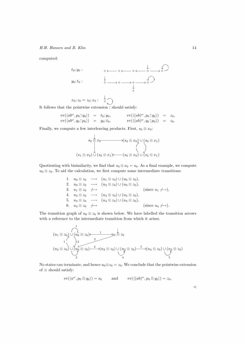
computed:
t0; y0 : ��◦ ◦oo ◦oo ◦oo // ◦
y0; t0 : ��◦ // ◦ // ◦
��
// ◦
◦
x0; z0 = z0;x0 : ��◦ dd
It follows that the pointwise extension ; should satisfy:
ev(〈abω, p0 ; q0〉) = t0; y0, ev(〈(ab)ω, p0 ; q0〉) = z0,
ev(〈abω, q0 ; p0〉) = y0; t0, ev(〈(ab)ω, q0 ; p0〉) = z0.
Finally, we compute a few interleaving products. First, s0 ⊗ x0:
��s0 ⊗ x0
//
��
(s2 ⊗ x0) ∪ (s0 ⊗ x1)
��(s1 ⊗ x0) ∪ (s0 ⊗ x1) (s0 ⊗ x0) ∪ (s2 ⊗ x1)oo
??
Quotienting with bisimilarity, we find that s0⊗x0 = s0. As a final example, we computeu0 ⊗ z0. To aid the calculation, we first compute some intermediate transitions:
1. u0 ⊗ z0 −→ (u1 ⊗ z0) ∪ (u0 ⊗ z0),2. u0 ⊗ z0 −→ (u2 ⊗ z0) ∪ (u0 ⊗ z0),3. u1 ⊗ z0 6−→ (since u1 6−→),4. u2 ⊗ z0 −→ (u3 ⊗ z0) ∪ (u2 ⊗ z0),5. u3 ⊗ z0 −→ (u4 ⊗ z0) ∪ (u3 ⊗ z0),6. u4 ⊗ z0 6−→ (since u4 6−→).
The transition graph of u0 ⊗ z0 is shown below. We have labelled the transition arrowswith a reference to the intermediate transition from which it arises.
��(u1 ⊗ z0) ∪ (u0 ⊗ z0)
1
��
2
��
u0 ⊗ z01oo
2
ttiiiiiiiiiiiiiiiiii
(u2 ⊗ z0) ∪ (u0 ⊗ z0)
2
YY
1
??
4 //(u3 ⊗ z0) ∪ (u2 ⊗ z0)
4
YY5 //(u4 ⊗ z0) ∪ (u3 ⊗ z0)
5
YY
No states can terminate, and hence u0⊗z0 = z0. We conclude that the pointwise extensionof ⊗ should satisfy:
ev(〈aω, p0 ⊗ q0〉) = s0 and ev(〈(ab)ω, p0 ⊗ q0〉) = z0.
�

Pointwise Extensions of GSOS-Defined Operations 15
In the above examples, pointwise extensions of operations were calculated on somespecific argument values. To check whether these pointwise extensions are well-definedin general, and whether they can be defined in a rule-based fashion as in Section 3, it isnecessary to understand those rule-based specifications in a general coalgebraic setting.This is the aim of the next section.
5. Distributive Laws and GSOS Rules
The equation- and rule-based definitions in the examples of Sections 3 and 4 are specialcases of a general framework for defining operations on final coalgebras, parameterizedboth by the behaviour functor F and the signature Σ of operations. The framework,developed in (Turi and Plotkin 1997), is based on the abstract notion of distributive law.
Basic distributive laws. Let F be a behaviour functor, 〈Z, ζ〉 the final F -coalgebra, andΣ an algebraic signature. A natural transformation λ : ΣF =⇒ FΣ, i.e. a distributivelaw of Σ over F , induces a Σ-algebra on Z by finality, as the unique F -coalgebra mapfrom λZ ◦ Σζ to 〈Z, ζ〉. This is illustrated in the following diagram:
ΣZΣζ
//
σ
��
ΣFZλZ // FΣZ
Fσ
��
Z ∼=
ζ// FZ
(12)
For instance, the definition of ⊕ in Example 3.1 induces a natural transformation
λ : (R×−)× (R×−) =⇒ R× (−×−)
(i.e. ΣX = X ×X and FX = R×X) whose X-component is given by:
λX : (R×X)× (R×X) =⇒ R× (X ×X)〈〈a, x1〉, 〈b, y1〉〉 7→ 〈a+ b, 〈x1, y1〉〉.
(13)
It is straightforward to check that the operation σ : Rω × Rω → Rω arising from this λas in (12), is the expected operation ⊕ induced by equations of Example 3.1 accordingto (Rutten 2003).
Monadic distributive laws. In specifications associated with basic distributive laws, allexpressions on the right-hand sides of rule conclusions must be Σ-terms of depth exactly1. Definitions of some useful operations do not conform to this restriction.
For an easy example, consider for FX = R×X a unary “head replacement” operationa/− : Rω → Rω, defined equivalently by equations or rules by:
hd(a/x0) = a
tl(a/x0) = tl(x0)i.e.
x0b→ x1
a/x0a→ x1
.
Note how the conclusion of the above rule is a variable, i.e., a term of depth 0 ratherthan 1. For this reason, the above definition does not correspond to a basic distributive
H.H. Hansen and B. Klin 16
law λ : ΣF =⇒ FΣ. There are also useful examples where the relevant terms have depthmore than 1 (see e.g. the interleaving operation in Example 4.5).
To deal with such examples, one can consider natural transformations of the typeρ : ΣF =⇒ FT ; these allow arbitrary Σ-terms where only terms of depth 1 were allowed.Such natural transformations induce Σ-operations on final F -coalgebras much the sameas basic distributive laws, as the unique maps σ : ΣZ → Z that make the diagram:
ΣZΣζ
//
σ
��
ΣFZρZ // FTZ
Fσ]
��
Z ∼=
ζ// FZ,
(14)
commute, where σ] is the T -algebra corresponding to σ as described in Section 2.2.An alternative way to understand this definition, and convince oneself that σ as above
indeed exists uniquely, is to observe that transformations ρ : ΣF =⇒ FT are in 1-1correspondence with distributive laws of the monad T over the endofunctor F , i.e.,natural transformations λ : TF =⇒ FT that respect the monad structure of T . Suchdistributive laws induce the algebraic structure σ] uniquely as in (12), with T substitutedfor Σ.
GSOS specifications. For an example that does not conform to either of the law typesexplained above, consider the definition of � in Example 3.2. It does not correspond toa natural transformation λ : ΣF =⇒ FΣ (for ΣX = X × X and FX = R × X), andintuitively, the reason for this is the use of the variable x0 on the right side of an equation,or in the target of the conclusion of a rule. However, that definition corresponds to a lawof the type
ρ : Σ(Id × F ) =⇒ FΣ
where ρ has X-component:
ρX : (X × R×X)× (X × R×X) =⇒ R× (X ×X)〈〈x0, a, x1〉, 〈y0, b, y1〉〉 7→ 〈a+ b, 〈x0, y1〉〉
(15)
One can also combine the expressivity of this type of laws with that of monadic distribu-tive laws described above, and consider the following definition:
Definition 5.1 A GSOS specification (of Σ over F ) is a natural transformation
ρ : Σ(Id × F ) =⇒ FT .
�
GSOS specifications are a particularly useful type of distributive laws, able to describemany interesting definitions. Their name comes from the fact that for the endofunctorFX = (PωX)A (see Example 2.6), they correspond (see Turi and Plotkin 1997; Bartels2004) to structural operational semantic specifications of LTSs in the well known GSOSformat (Aceto et al. 2001).
Pointwise Extensions of GSOS-Defined Operations 17
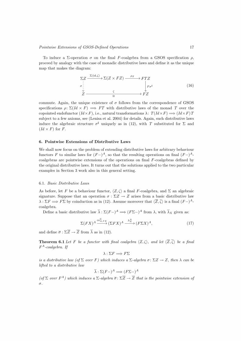
To induce a Σ-operation σ on the final F -coalgebra from a GSOS specification ρ,proceed by analogy with the case of monadic distributive laws and define it as the uniquemap that makes the diagram:
ΣZΣ〈id,ζ〉
//
σ
��
Σ(Z × FZ)ρZ // FTZ
Fσ]
��
Z ∼=
ζ// FZ
(16)
commute. Again, the unique existence of σ follows from the correspondence of GSOSspecifications ρ : Σ(Id × F ) =⇒ FT with distributive laws of the monad T over thecopointed endofunctor (Id×F ), i.e., natural transformations λ : T (Id×F ) =⇒ (Id×F )Tsubject to a few axioms, see (Lenisa et al. 2004) for details. Again, such distributive lawsinduce the algebraic structure σ] uniquely as in (12), with T substituted for Σ and(Id × F ) for F .
6. Pointwise Extensions of Distributive Laws
We shall now focus on the problem of extending distributive laws for arbitrary behaviourfunctors F to similar laws for (F−)A, so that the resulting operations on final (F−)A-coalgebras are pointwise extensions of the operations on final F -coalgebras defined bythe original distributive laws. It turns out that the solutions applied to the two particularexamples in Section 3 work also in this general setting.
6.1. Basic Distributive Laws
As before, let F be a behaviour functor, 〈Z, ζ〉 a final F -coalgebra, and Σ an algebraicsignature. Suppose that an operation σ : ΣZ → Z arises from a basic distributive lawλ : ΣF =⇒ FΣ by coinduction as in (12). Assume moreover that 〈Z, ζ〉 is a final (F−)A-coalgebra.
Define a basic distributive law λ : Σ(F−)A =⇒ (FΣ−)A from λ, with λX given as:
Σ(FX)AcsΣ
A,FX// (ΣFX)A
λAX // (FΣX)A, (17)
and define σ : ΣZ → Z from λ as in (12).
Theorem 6.1 Let F be a functor with final coalgebra 〈Z, ζ〉, and let 〈Z, ζ〉 be a finalFA-coalgebra. If
λ : ΣF =⇒ FΣ
is a distributive law (of Σ over F ) which induces a Σ-algebra σ : ΣZ → Z, then λ can belifted to a distributive law
λ : Σ(F−)A =⇒ (FΣ−)A
(of Σ over FA) which induces a Σ-algebra σ : ΣZ → Z that is the pointwise extension ofσ.

H.H. Hansen and B. Klin 18
Proof. Define λ by (17) and see the Appendix.
Example 6.2 Let us calculate λ for the law λ in (13) which defines the operation⊕ : Rω×Rω → Rω from Example 3.1. The syntax and behaviour functors are ΣX = X×Xand FAX = (R×X)R, hence an X-component of λ is of the type:
λX : (R×X)R × (R×X)R =⇒ (R×X ×X)R.
Below, for φ ∈ (R × X)R and a ∈ R, we denote the projections of φ(a) by φ0(a) andφ1(a), i.e., φ(a) = 〈φ0(a), φ1(a)〉. Instantiating (17) and (13), λX is defined by:
〈φ, ψ〉_
��
∈ (R×X)R × (R×X)R
csΣR,R×X
��
λa.〈φ0(a), φ1(a), ψ0(a), ψ1(a)〉_
��
∈ (R×X × R×X)R
λRX
��
λa.〈φ0(a) + ψ0(a), 〈φ1(a), ψ1(a)〉〉 ∈ (R×X ×X)R
Formulating the above λ as an inference rule we recognise the rule for ⊕ in (5), withb = φ0(a), c = ψ0(a), x1 = φ1(a) and y1 = ψ1(a). �
It should be noted that the same construction works for the more expressive type ofspecifications ρ : ΣF =⇒ FT . To define the pointwise extension of an operation definedby such a specification, first obtain from ρ a monadic distributive law λ : TF =⇒ FT , andthen apply the construction (17) and Theorem 6.1, with Σ replaced by T throughout.
6.2. GSOS Specifications
We shall now move to define pointwise extensions of operations defined by GSOS speci-fications ρ : Σ(Id × F ) =⇒ FT .
First, note that unlike in the case of monadic distributive laws above, one cannot usethe correspondence of GSOS specifications and distributive laws of T over Id × F , andapply (17) and Theorem 6.1 with Σ replaced by T and F replaced by Id×F throughout.The reason for this is that in the natural transformation λ obtained from (17) in thiscase, an X-component has domain T (X × FX)A, and not T (X × (FX)A) as requiredto define the pointwise extension operation by (16).
It seems that the problem can be circumvented by precomposing the counterpartof (17) with an appropriate (co)strength. In this way, from a GSOS specification ρ,one obtains a GSOS specification ρ : Σ(Id × (F−)A) =⇒ (FT )A with ρX defined by:
Σ(X × (FX)A)cs
Σ(X×−)A,FX
// (Σ(X × FX))AρA
X // (FTX)A, (18)
and proceeds to define an extended operation σ : ΣZ → Z from (16).However, it turns out that σ obtained this way is not the pointwise extension of the
operation σ : ΣZ → Z, i.e., the relevant diagram (11) does not commute. Indeed, one

Pointwise Extensions of GSOS-Defined Operations 19
may repeat the development of Example 6.2 for (18) with ρ defined by (15), and realisethat the resulting ρ corresponds to the rule (6), which does not define the pointwiseextension of � as we saw in Example 3.2.
To treat the case of arbitrary GSOS specifications correctly, we proceed in a moresubtle way, by analogy with the development of Example 3.2. First, extend the syntax Σby defining
Σ . = A×− Σ = Σ + Σ . .
This amounts to adding |A| auxiliary unary operations to the syntax. In examples, wewill denote these operations by a .−, for a ∈ A. Their semantics will intuitively be“one-element buffer” operations. Let T be the free monad over Σ.
The pointwise extension of σ will be defined with the help of an algebra σ : ΣZ → Z
such that the diagram:
Aω × ΣZ
id×ιZ��
stΣAω,Z
// Σ(Aω × Z)Σev // ΣZ
σ
��
Aω × ΣZ
id×σ��
Aω × Z ev// Z
(19)
commutes (compare (11)), where ι : Σ → Σ is the coproduct injection. To define σ weprovide a GSOS specification ρ : Σ(Id × (F−)A) =⇒ (F T−)A, by cases of Σ: for Σ . ,
A× (X × (FX)A)π13 // A× (FX)A
εFX // FX EDBC ηFX
GF��(A× FX)A
(stFA,X)A
// (F (A×X))A � � // (F TX)A
(20)
and for Σ,
Σ(X × (FX)A)Σ(ηX×id)
// Σ((A×X)A × (FX)A) EDBC csΣ(−×−)A,A×X,FX
GF��(Σ(A×X × FX))A � � // (Σ((A×X +X)× F (A×X +X)))A EDBC ρA
A×X+X
GF��(FT (A×X +X))A � � // (F TX)A
(21)
This ρ defines an algebra σ : ΣZ → Z as usual, by (16). With some straightforward,albeit tedious, diagram chasing one shows that (19) commutes:
Theorem 6.3 Let F be a functor with final coalgebra 〈Z, ζ〉, and let 〈Z, ζ〉 be a final

H.H. Hansen and B. Klin 20
FA-coalgebra. If
ρ : Σ(Id × F−) =⇒ (FT−)
is a GSOS specification (of Σ over F ) which induces a Σ-algebra σ : ΣZ → Z, then ρ canbe lifted to a GSOS specification
ρ : Σ(Id × (F−)A) =⇒ (F T−)A
(of Σ over FA) which induces a Σ-algebra σ : ΣZ → Z such that σ ◦ ιZ : ΣZ → Z is thepointwise extension of σ.
Proof. Define ρ by (20) and (21) and see the Appendix.
We illustrate the construction behind Theorem 6.3 using the operation � from Exam-ple 3.2.
Example 6.4 Let us calculate ρ : Σ(Id × (F−)A) =⇒ (F T−)A for the law ρ in (15)which defines the operation � : Rω × Rω → Rω. The syntax and behaviour functors areΣX = X ×X and FAX = (R×X)R, hence Σ .X = R×X, ΣX = (X ×X) + (R×X)and ρ is of type
ρ : Σ(Id × (R×−)R) =⇒ (R× T−)R.
The two cases for ρ have X-components:
ρ .X : R×X × (R×X)R → (R× TX)R
ρΣX : Σ(X × (R×X)R) → (R× TX)R
given by (20) and (21), respectively. Intuitively, ρ . specifies the FA-behaviour of thebuffer operations and ρΣ specifies the FA-behaviour of the Σ-operation.
Again, for φ ∈ (R ×X)R we let φ0 and φ1 be defined by φ(a) = 〈φ0(a), φ1(a)〉 for alla ∈ R. To ease the notational burden, we shall suppress some coproduct injections andtreat them as set inclusions.

Pointwise Extensions of GSOS-Defined Operations 21
For ρ . , (20) instantiates to:
〈a, x, φ〉_
��
∈ R× (X × (R×X)R)
π13
��
〈a, φ〉_
��
∈ R× (R×X)R
εR×X
��
〈φ0(a), φ1(a)〉_
��
∈ R×X
ηR×X
��
λc.〈c, 〈φ0(a), φ1(a)〉〉_
��
∈ (R× (R×X))R
(stR×−R,X )R
��
λc.〈φ0(a), 〈c, φ1(a)〉〉 ∈ (R× (R×X))R� _
��
λc.〈φ0(a), 〈c, φ1(a)〉〉 ∈ (R× TX)R
The last step involves the inclusion of R ×X = Σ .X into TX. So 〈c, φ1(a)〉 should beread as c . φ1(a). Formulating ρ . as a GSOS rule we recognise the rule for a . x0 in (9)(with b = φ0(a), x0 = x and x1 = φ1(a)).
For ρΣ, (21) instantiates to:
〈〈x, φ〉, 〈y, ψ〉〉_
��
∈ (X × (R×X)R)2
Σ(ηX×id)
��
〈〈λa.〈a, x〉, φ〉, 〈λa.〈a, y〉, ψ〉〉_
��
∈ ((R×X)R × (R×X)R)2
csΣ(−×−)R,R×X,R×X
��λa.〈〈〈a, x〉, 〈φ0(a), φ1(a)〉〉,〈〈a, y〉, 〈ψ0(a), ψ1(a)〉〉〉 ∈ (((R×X)× (R×X))2)R
� _
��λa.〈〈〈a, x〉, φ0(a), φ1(a)〉,〈〈a, y〉, ψ0(a), ψ1(a)〉〉
_
��
∈ (((R×X +X)× R× (R×X +X))2)R
ρRR×X+X
��
λa.〈φ0(a) + ψ0(a), 〈〈a, x〉, ψ1(a)〉〉 ∈ (R× T (R×X +X))R� _
��
λa.〈φ0(a) + ψ0(a), 〈〈a, x〉, ψ1(a)〉〉 ∈ (R× T (X))R
H.H. Hansen and B. Klin 22
The last step involves the natural inclusion of terms induced by mapping a pair 〈a, x〉 ∈R×X to the buffer expression a . x ∈ Σ .X ⊆ TX. With this inclusion in mind, we seethat the rule for � in (9) is the rule-based formulation of ρΣ. �
Informally, ρΣ can be described as obtained from ρ by replacing all occurrences ofx0 ∈ X on the right-hand sides with a . x0 and adding input labels to arrows. In the nextsection we will see more examples of how ρ is obtained from ρ.
7. Further Examples
We shall now sketch a few more example applications of the constructions and results ofSection 6.
Example 7.1 Taking F = 2 × − and A = 2, (2 × −)-behaviours are bitstreams and(2 × −)2-coalgebras are binary Mealy machines whose behaviours are causal bitstreamfunctions (cf. Examples 2.1 and 2.2). In (Hansen and Rutten 2010), a coalgebraic treat-ment was given of the so-called 2-adic bitstream operations and their pointwise extensionsto causal bitstream functions. The main purpose in (Hansen and Rutten 2010) was toconstruct binary Mealy machine realisations from 2-adic function expressions. A cru-cial step in this result consists of showing that 2-adic function expressions can be given aMealy machine structure. It was, however, not clear whether this Mealy machine of termscomes about from the existence of a distributive law. A reason for this is that the bufferoperations were not explicitly used in (Hansen and Rutten 2010), and so the generalpicture did not emerge. Since the 2-adic bitstream operations are defined in the GSOSformat, Theorem 6.3 tells us that a distributive law exists and how to derive it. We nowpresent this distributive law, except that we leave out the (guarded) inverse operationin order to simplify the presentation. It is straightforward to apply Theorem 6.3 to alsoinclude the inverse.
The 2-adic bitstream operations arise from viewing (a0, a1, a2, . . .) ∈ 2ω as the coef-ficients of the power series representation of the 2-adic integer
∑ωi=0 ai2
i (cf. Koblitz1984). The 2-adic integers include the set Qodd of rational numbers with odd denomina-tor via the map B : Qodd → 2ω which converts numbers to their base 2 representation.For a positive integer n, B(n) is simply obtained by writing n in binary and paddingwith a tail of zeros, e.g. B(6) = (0, 1, 1, 0, 0, 0, . . .). Negative integers are represented bytaking an infinitary version of two’s complement, e.g. B(−6) = (0, 1, 0, 1, 1, 1, . . .). Moregenerally, for any q ∈ Qodd , B(q) is an eventually periodic bitstream.
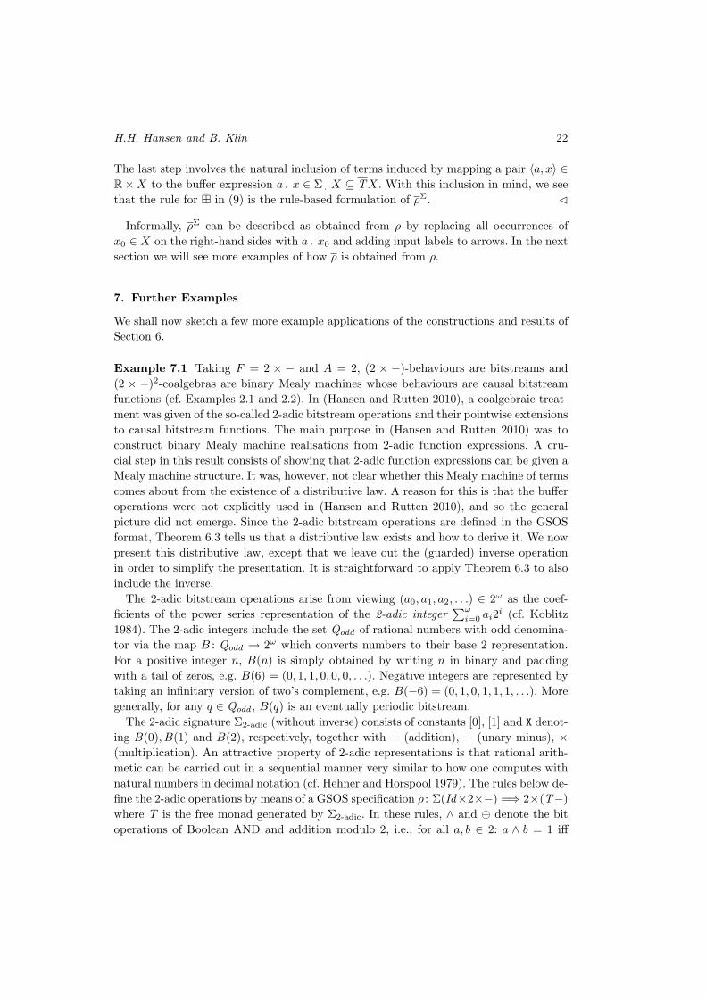
The 2-adic signature Σ2-adic (without inverse) consists of constants [0], [1] and X denot-ing B(0), B(1) and B(2), respectively, together with + (addition), − (unary minus), ×(multiplication). An attractive property of 2-adic representations is that rational arith-metic can be carried out in a sequential manner very similar to how one computes withnatural numbers in decimal notation (cf. Hehner and Horspool 1979). The rules below de-fine the 2-adic operations by means of a GSOS specification ρ : Σ(Id×2×−) =⇒ 2×(T−)where T is the free monad generated by Σ2-adic. In these rules, ∧ and ⊕ denote the bitoperations of Boolean AND and addition modulo 2, i.e., for all a, b ∈ 2: a ∧ b = 1 iff

Pointwise Extensions of GSOS-Defined Operations 23
a = b = 1 and a⊕ b = 1 iff a 6= b.
[0] 0→ [0] [1] 1→ [0] X 0→ [1]
x0b→ x1 y0
c→ y1
x0 + y0b⊕c→ (x1 + y1) + [b ∧ c]
x0b→ x1
−x0b→ −(x1 + [b])
x0b→ x1 y0
c→ y1
x0 × y0b∧c→ (x1 × y0) + ([b]× y1)
The rule for + shows that carry bits may propagate infinitely to the right, for example(1, 0, 0, 0, . . .) + (1, 1, 1, . . .) = (0, 0, 0, . . .), and the rule for × shows that multiplicationis done in the usual shift-add manner. We refer to (Hansen and Rutten 2010) for moredetails.
In order to be able to specify bitstream functions rather than just bitstreams, thesyntax is extended with a variable s. The 2-adic function expressions is thus the setT ({s}) of Σ2-adic-terms freely generated over the single variable s. Algebraically, a termt in T ({s}) is evaluated in Γ by interpreting s as the identity map id: 2ω → 2ω, andthe 2-adic operations as their pointwise extensions to Γ. The fact that we can define thepointwise extensions with a distributive law implies that the coalgebraic semantics of2-adic function expressions coincides with the algebraic semantics. The pointwise exten-sions of [0], [1], X,+ and − to the binary Mealy functor (2 × −)2 are obtained from thesimple format in (17) and its monadic version. The pointwise extension of multiplication,however, requires the use of the buffer operations. We omit the overline notation andsimply write + instead of + etc. The typing should be clear from the context.
[0] a|0→ [0] [1] a|1→ [0] Xa|0→ [1]
x0a|b→ x1 y0
a|c→ y1
x0 + y0a|b⊕c→ (x1 + y1) + [b ∧ c]
x0a|b→ x1
−x0a|b→ −(x1 + [b])
x0a|b→ x1 y0
a|c→ y1
x0 × y0a|b∧c→ (x1 × (a . y0)) + ([b]× y1)
x0a|b→ x1
a . x0c|b→ c . x1
Interestingly, it was possible to define the Mealy machine of terms in (Hansen and Rutten2010), without adding the buffer operations, since these can already be expressed in theexisting syntax: for every term t ∈ T ({s}) and every a ∈ 2, there is a term, denoted byt(a :s) ∈ T ({s}), such that for all input streams α ∈ 2ω, beh(t(a :s))(α) = beh(t)(a :α) =beh(a . t)(α). We refer to (Hansen and Rutten 2010) for more details on the definition oft(a :s). �
Example 7.2 Consider the functor FX = 1+X from Example 2.3, that is, F -behavioursare the extended natural numbers N + {ω}, and FA-behaviours are non-empty, prefix-closed languages (cf. Examples 2.3 and 2.4). The operations max (∨), plus (+) andtimes (·) on the extended natural numbers (cf. Example 4.4) are induced by the following

H.H. Hansen and B. Klin 24
rules:
x0 → x1 y0 → y1
x0 ∨ y0 → x1 ∨ y1
x0 → x1 y0 → ⊥x0 ∨ y0 → x1
x0 → ⊥ y0 → y1
x0 ∨ y0 → y1
x0 → x1
x0 + y → x1 + y
x0 → ⊥ y0 → y1
x0 + y0 → y1
x0 → ⊥ y0 → ⊥x0 + y0 → ⊥
x0 → x1 y0 → y1
x0 · y0 → (x1 · y0) + y1
x0 → ⊥x0 · y → ⊥
y0 → ⊥x · y0 → ⊥
The pointwise extensions of these operations to the final FA-coalgebra are defined by thefollowing set of rules. Again, we omit the overline notation for the pointwise extendedoperations.
x0a→ x1
a . x0b→ b . x1
x0a→ ⊥
a . x0b→ ⊥
x0a→ x1 y0
a→ y1
x0 ∨ y0a→ x1 ∨ y1
x0a→ x1 y0
a→ ⊥x0 ∨ y0
a→ x1
x0a→ ⊥ y0
a→ y1
x0 ∨ y0a→ y1
x0a→ x1
x0 + y a→ x1 + (a . y)x0
a→ ⊥ y0a→ y1
x0 + y0a→ y1
x0a→ ⊥ y0
a→ ⊥x0 + y0
a→ ⊥
x0a→ x1 y0
a→ y1
x0 · y0a→ (x1 · (a . y0)) + y1
x0a→ ⊥
x0 · y a→ ⊥y0
a→ ⊥x · y0
a→ ⊥
To illustrate, let A = {a, b} and for n ∈ N, let an = {ε, a, aa, . . . , an}, that is, an denotesthe prefix-closed language generated by an. We then have for all n ∈ N,
an+1 a→ an, a0 a→ ⊥, an c→ ⊥ if c 6= a.
Applying the rule for buffer expressions, we find that for all c, d ∈ A,
a . an+1 c→ c . an, c . a . an+1 d→ d . c . an, etc.
In general, for all k ∈ N and c1, . . . , ck ∈ A,
ck−1 . . . . c1 . a . an+1 ck→ ck . ck−1 . . . . c1 . a
n, andck−1 . . . . c1 . a . a
0 ck→ ⊥
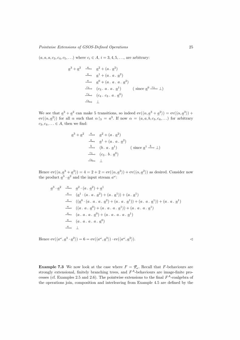
Let us check the pointwise extension of + on a3 and a2. For any stream α ∈ Aω thatstarts with three a’s, i.e. α�3 = a3, we have ev(〈α, a3〉) + ev(〈α, a2〉) = 3 + 2 = 5. We nowuse the above rules to compute the transitions that can be made by a3 + a2 on input
Pointwise Extensions of GSOS-Defined Operations 25
(a, a, a, c3, c4, c5, . . .) where ci ∈ A, i = 3, 4, 5, . . ., are arbitrary:
a3 + a2 a→ a2 + (a . a2)a→ a1 + (a . a . a2)a→ a0 + (a . a . a . a2)c3→ (c3 . a . a . a1) ( since a0 c3→ ⊥)c4→ (c4 . c3 . a . a0)c5→ ⊥
We see that a3 + a2 can make 5 transitions, so indeed ev(〈α, a3 + a2〉) = ev(〈α, a3〉) +ev(〈α, a2〉) for all α such that α �3 = a3. If now α = (a, a, b, c3, c4, . . .) for arbitraryc3, c4, . . . ∈ A, then we find:
a3 + a2 a→ a2 + (a . a2)a→ a1 + (a . a . a2)b→ (b . a . a1) ( since a1 b→ ⊥)c3→ (c3 . b . a0)c4→ ⊥
Hence ev(〈α, a3 + a2〉) = 4 = 2 + 2 = ev(〈α, a3〉) + ev(〈α, a2〉) as desired. Consider nowthe product a3 · a2 and the input stream aω:
a3 · a2 a→ a2 · (a . a2) + a1
a→ (a1 · (a . a . a2) + (a . a1)) + (a . a1)a→ ((a0 · (a . a . a . a2) + (a . a . a1)) + (a . a . a1)) + (a . a . a1)a→ ((a . a . a0) + (a . a . a . a1)) + (a . a . a . a1)a→ (a . a . a . a0) + (a . a . a . a . a1)a→ (a . a . a . a . a0)a→ ⊥
Hence ev(〈aω, a3 · a2〉) = 6 = ev(〈aω, a3〉) · ev(〈aω, a2〉). �
Example 7.3 We now look at the case where F = Pω. Recall that F -behaviours arestrongly extensional, finitely branching trees, and FA-behaviours are image-finite pro-cesses (cf. Examples 2.5 and 2.6). The pointwise extensions to the final FA-coalgebra ofthe operations join, composition and interleaving from Example 4.5 are defined by the
H.H. Hansen and B. Klin 26
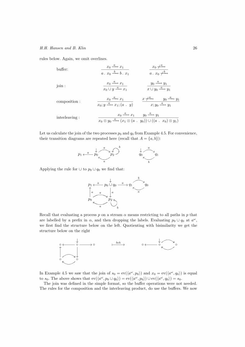
rules below. Again, we omit overlines.
buffer:x0
a→ x1
a . x0b→ b . x1
x0 6 a→a . x0 6 b→
join :x0
a→ x1
x0 ∪ y a→ x1
y0a→ y1
x ∪ y0a→ y1
composition :x0
a→ x1
x0; y a→ x1; (a . y)x 6 a→ y0
a→ y1
x; y0a→ y1
interleaving :x0
a→ x1 y0a→ y1
x0 ⊗ y0a→ (x1 ⊗ (a . y0)) ∪ ((a . x0)⊗ y1)
Let us calculate the join of the two processes p0 and q0 from Example 4.5. For convenience,their transition diagrams are repeated here (recall that A = {a, b}):
�� ��p1 p0
aoo
a
""p2
a
bb
b
q0
a
""q1
b
aa
Applying the rule for ∪ to p0 ∪ q0 we find that:
��p1 p0 ∪ q0
aoo a //
a
��
q1
b
""q0
a
aa
p0
a
$$
a
OO
p2
a
dd
b
kk
Recall that evaluating a process p on a stream α means restricting to all paths in p thatare labelled by a prefix in α, and then dropping the labels. Evaluating p0 ∪ q0 at aω,we first find the structure below on the left. Quotienting with bisimilarity we get thestructure below on the right
�� ��◦ ◦oo //
��
◦ � beh // ◦ ◦!!
oo ◦aa
◦!!
OO
◦aa
In Example 4.5 we saw that the join of s0 = ev(〈aω, p0〉) and x0 = ev(〈aω, q0〉) is equalto s0. The above shows that ev(〈aω, p0 ∪ q0〉) = ev(〈aω, p0〉) ∪ ev(〈aω, q0〉) = s0.
The join was defined in the simple format, so the buffer operations were not needed.The rules for the composition and the interleaving product, do use the buffers. We now

Pointwise Extensions of GSOS-Defined Operations 27
compute part of the transition structure of p0; q0. In order to keep a compact notation, wewill write w .x instead of a1 . . . . . an . x when w = a1 . . . an. Dots after a node indicatethat it has outgoing transitions that are not shown.
��a . q1 p1; (a . q0)
aoo
b
��
p0; q0aoo a // p2; (a . q0)
a
��
b // p2; (ba . q0)b //
a
��
. . .
a . q0
a
OO
b
%%
b . q1
a
dd
b
��
(ba . q1) p0; (a2 . q0)
a
��
boo
a
xxrrrrrrrrrrp0; (aba . q0) . . .
b . q0 p1; (a3 . q0)
a
zzuuuuuuuuuub
��
p2; (a3 . q0)
a
��
b // p2; (ba3 . q0) . . .
a3 . q1 ba2 . q1 p0; (a4 . q0)
a
xxrrrrrrrrrra
��
b // ba3 . q1
p1; (a5 . q0)
a
zzuuuuuuuuuub
��
p2; (a5 . q0)b //
a
��
p2; (ba5 . q0) . . .
a5 . q1 ba4 . q1 p0; (a6 . q0) . . .
From the above, it is fairly easy to see that evaluating p0; q0 at aω yields a structurebisimilar to the one below on the left. Quotienting further with bisimilarity, we getthe structure on the right, which is equal to s0;x0 where s0 = ev(〈aω, p0〉) and x0 =ev(〈aω, q0〉) (cf. Example 4.5), hence ev(〈aω, p0; q0〉) = ev(〈aω, p0〉); ev(〈aω, q0〉).
�� ��◦ ◦oo ◦oo // ◦
zzuuuuu� beh // ◦ ◦oo ◦oo
��◦\\
◦ ◦oo ◦oo // ◦XX
As another example, we compute the transitions of p0; q0 on abω:
// p0; q0
a ))RRRRRRRa // p2; (a . q0)
b // p2; (ba . q0)b // p2; (b2a . q0)
b // . . .
p1; (a . q0)b // b . q1
b // b . q0
Removing the labels results in a tree which is bisimilar to t0; y0 where t0 = ev(〈abω, p0〉)and y0 = ev(〈abω, q0〉) (cf. Example 4.5), and so indeed we have ev(〈abω, p0; q0〉) =ev(〈abω, p0〉); ev(〈abω, q0〉). Note that the naive approach to defining the operation ; onFA-behaviours would lead to the following behaviour on abω:

H.H. Hansen and B. Klin 28
// p0; q0
a ))RRRRRRa // p2; q0
b // p2; q0b // p2; q0
b // . . .
p1; q0
If we remove the labels, we obtain a tree which is clearly not bisimilar to t0; y0. We leaveit to the reader to check that for α ∈ {aω, abω, (ab)ω}, ev(〈α, p0 ⊗ q0〉) = ev(〈α, p0〉) ⊗ev(〈α, q0〉). �
8. Conclusions and Future Work
We have shown how GSOS rules that define operations on F -behaviours can be lifted toGSOS rules that define the corresponding pointwise extensions on FA-behaviours. Theconstruction is carried out uniformly for all behaviour functors F and it relies on extend-ing the signature with a family of buffer operations. Although the proof is technicallyinvolved, applying the construction to concrete examples is straightforward. Our originalmotivating example was the pointwise extension of the 2-adic operations on bitstreams tocausal bitstream functions (Mealy machine behaviours) from (Hansen and Rutten 2010).In this example, a specification language for bitstreams is turned into one for bitstreamfunctions by adding a variable to the syntax as in standard mathematical practice. Weexpect that this ‘trick’ is useful in other settings. In this perspective, our result can beformulated as: a structural operational semantics for Σ-expressions can be systematicallylifted to one for Σ-function expressions in such a way that the operational (coalgebraic)semantics coincides with the algebraic semantics.
As related work we mention (Jacobs 2006), where it is shown that an Eilenberg-Moorealgebra σ : TB → B for a monad T induces a distributive law of T over the (Moore)functor FX = B × XA, and the Eilenberg-Moore algebra induced on the carrier BA
∗
of the final F -coalgebra is the pointwise extension of σ. Due to the shape of the functorFX = B × XA, our present result does not directly relate to that in (Jacobs 2006),however, it is straightforward to state and prove an analogous one: If σ : TB → B isan Eilenberg-Moore algebra, then σ gives rise to a distributive law of T over the Mealyfunctor (B × −)A such that the induced Eilenberg-Moore algebra σ : T (BA
+) → BA
+
is the pointwise extension of σ. Note that causal stream functions Aω → Bω are in 1-1correspondence with functions A+ → B. In our setting, we can describe the pointwiseextension of σ in two steps. First, from σ it is easy to define a simple distributive law λ
of T over the functor (B × −). The element-wise addition of streams over R is such anexample. This λ defines an operation σω on Bω which is the pointwise (i.e. element-wise)extension of σ. Second, we apply Theorem 6.1 to lift λ and obtain the pointwise extensionσω on Γ. One easily shows that σω corresponds to σ under the bijection Γ ∼= BA
+.
As mentioned in Section 4, the input evaluation s n m is a construction very similarto the wreath product of automata (cf. Carton 2000; Pin and Weil 2002; Straubing1989). The wreath product exists for different types of automata, but the basic ideain all of them is that the output of the one automaton becomes the input of the other.Several results in formal language theory have been proved using the wreath product. For

Pointwise Extensions of GSOS-Defined Operations 29
example, taking the wreath product of a finite deterministic automaton and a sequentialtransducer, one easily concludes that sequential functions preserve regularity of languagesunder inverse images. Deeper results formulated in terms of decomposition of semigroupsinclude the Krohn-Rhodes theorem and characterisations of concatenation hierarchies.We refer to (cf. Carton 2000; Pin and Weil 2002; Straubing 1989) for further referencesto the literature. It would be interesting to study wreath products more generally in acoalgebraic setting, and explore their applicability in the coalgebraic theory of formallanguages (cf. Rutten 2003).
Another observation of the n-operation, is that it suggests a characterisation of FA-behaviours as causal functions f from Aω to F -behaviours. Here, we call f causal if forall n ∈ N, α�n= β�n implies that f(α) and f(β) are n-step bisimilar. We leave the detailsof such a characterisation for future work.
Appendix A. Proofs
A.1. Preliminaries
We begin with some basic results and definitions that will be useful in the following.For any functor F , strength stF and costrength csF (see Section 2.1) correspond to
each other via the adjunction A×− a (−)A. In particular, there is a commuting diagram:
A× F (XA)stF
A,XA//
id×csFA,X
��
F (A×XA)
FεX
��
A× (FX)A εF X
// FX.
(22)
Strength respects products: there is
stFA×B,X = stFA,B×X ◦(idA × stFB,X). (23)
Strength transformations compose along functor composition: for endofunctors F and Gon Set, there is
stGFA,X = G stFA,X ◦ stGA,FX (24)
for any A and X. Strength is natural also in the endofunctor F . Indeed, for any naturaltransformation α : F =⇒ G, there is:
A× FXstF
A,X//
id×αX
��
F (A×X)
αA×X
��
A×GXstG
A,X
// G(A×X).
(25)
To simplify the notation, we will sometimes use a natural transformation e : Aω ×(−)A =⇒ Aω ×−, with the component eX defined by:
Aω ×XA〈tl,hd〉×id
// Aω ×A×XAid×εX // Aω ×X. (26)

H.H. Hansen and B. Klin 30
With this, the definition (10) of the map ev can be rewritten as:
Aω × Zev //
id×ζ��
Z
ζ
��
Aω × (FZ)A
eFZ
��
Aω × FZ
stFAω,Z
��
F (Aω × Z)Fev
// FZ.
(27)
A.2. Proof of Theorem 6.1
Recall that λ is defined by (17), and σ is defined from λ as in (12), specifically by:
ΣZΣζ
//
σ
��
Σ(FZ)AλZ // (FΣZ)A
(Fσ)A
��
Z ∼=
ζ// (FZ)A.
(28)
We shall prove that (11) commutes. To this end, define an F -coalgebra structure onAω × ΣZ:
Aω × ΣZid×Σζ
// Aω × Σ(FZ)Aid×λZ // Aω × (FΣZ)A EDBC eFΣZ
GF��
Aω × FΣZstF
Aω,ΣZ// F (Aω × ΣZ)
and check that both sides of (11) are coalgebra morphisms from it to the final F -

Pointwise Extensions of GSOS-Defined Operations 31
coalgebra. For the southwestern side, check the diagram:
Aω × ΣZid×σ
//
id×Σζ
��
Aω × Zev //
id×ζ
��
(i)
Z
ζ
��
(ii)
Aω × Σ(FZ)A
id×λZ
��
Aω × (FΣZ)Aid×(Fσ)A
//
eFΣZ
��
(iii)
Aω × (FZ)A
eFZ
��
Aω × FΣZid×Fσ
//
stFAω,ΣZ
��
(iv)
Aω × FZ
stFAω,Z
��
F (Aω × ΣZ)F(id×σ)
// F (Aω × Z)Fev
// FZ
where (i) commutes by (28), (ii) by (27), (iii) by naturality of e and (iv) by naturalityof stF .
For the northeastern side of (11), in the diagram:
Aω × ΣZ
id×Σζ
��
stΣAω,Z
//
(i)
Σ(Aω × Z)Σev //
Σ(id×ζ)��
ΣZσ //
Σζ
��
(iii)
Z
ζ
��
Aω × Σ(FZ)A
id×csΣA,FZ ((QQQQQQQQQQQQ
stΣAω,(FZ)A
//
id×λZ
��
Σ(Aω × (FZ)A)
ΣeFZ
��
(ii)
(v)
Aω × (ΣFZ)A
eΣFZ
��
id×λAZ
vvmmmmmmmmmmmm
Aω × (FΣZ)A
eFΣZ
��
Aω × ΣFZ
id×λZvvmmmmmmmmmmmmm
stΣAω,FZ
// Σ(Aω × FZ)
Σ stFAω,Z
��
Aω × FΣZ
stFAω,ΣZ
��
(vi) ΣF (Aω × Z)ΣFev //
λAω×Z
��
(iv)
ΣFZ
λZ
��
F (Aω × ΣZ)F stΣ
Aω,Z
// FΣ(Aω × Z)FΣev
// FΣZFσ
// FZ
(i) commutes by naturality of stΣ, (ii) by (27), (iii) by (12), (iv) by naturality of λ, (v)follows from (22) and (26) using naturality of stΣ and (23), and (vi) follows from (24)–(25); the remaining parts commute due to naturality of e and the definition of λ in (17).qed

H.H. Hansen and B. Klin 32
A.3. Proof of Theorem 6.3
We shall now prove that (19) commutes, recalling that ev is defined by (27) and σ isdefined from ρ as in (16), specifically by:
ΣZΣ〈id,ζ〉
//
σ
��
Σ(Z × (FZ)A)ρZ // (F T Z)A
(Fσ])A
��
Z ∼=
ζ// (FZ)A,
(29)
where ρ is defined by (20) and (21).In the proof, we shall use an auxiliary natural transformation
θ : Aω × Σ− =⇒ (Σ + Id)(Aω ×−)
with θX defined by cases of Σ: for Σ . ,
Aω ×A×X〈tl,hd〉−1×id
// Aω ×X � � // (Σ + Id)(Aω ×X)
and for Σ,
Aω × ΣXstΣ
Aω,X// Σ(Aω ×X) � � // (Σ + Id)(Aω ×X) .
The diagram (19) can be decomposed as:
Aω × ΣZ
id×ιZ��
stΣAω,Z
// Σ(Aω × Z)� _
��
Σev // ΣZ� _
��
Aω × ΣZ
id×σ��
θZ // Σ(Aω × Z) + (Aω × Z)Σev+ev
// ΣZ + Z
[σ,id]
��
Aω × Z ev// Z,
(30)
where the top left square commutes by the second clause of definition of θ, and thetop right square commutes obviously. In the following we shall prove that the bottomrectangle commutes as well.
To this end, consider a map γ : Aω × ΣZ → F (Aω × T Z) defined by:
Aω × ΣZid×Σ〈id,ζ〉
// Aω × Σ(Z × (FZ)A)id×ρZ // Aω × (F T Z)A EDBC eFT Z
GF��
Aω × F T ZstF
Aω,T Z// F (Aω × T Z).
Note that in this definition all maps except the first one are natural in Z. This allowsus to use a definition/proof principle similar to that used in (14), and infer that bothsides of the lower part of (30) are equal if they are both “maps” from γ to the final

Pointwise Extensions of GSOS-Defined Operations 33
F -coalgebra ζ in the following sense:
Aω × ΣZ
γ
��
id×σ// Aω × Z
ev // Z
ζ
��
F (Aω × T Z)F(id×σ])
// F (Aω × Z)Fev
// FZ
(31)
Aω × ΣZ
γ
��
θZ // Σ(Aω × Z) + (Aω × Z)Σev+ev
// ΣZ + Z[σ,id]
// Z
ζ
��
F (Aω × T Z)Fθ]
Z
// FT (Aω × Z)FTev
// FTZFσ]
// FZ
(32)
where θ] : Aω × T− =⇒ T (Aω ×−) is the obvious inductive extension of θ. The abovetwo conditions can equivalently be understood as two coalgebra morphism diagrams toζ from an F -coalgebra on Aω × T Z easily defined from γ; however, they are are a biteasier to prove in the present formulation.
The condition (31) is proved by analogy with the corresponding condition in the proofof Theorem 6.1; chase the diagram:
Aω × ΣZid×σ
//
id×Σ〈id,ζ〉��
Aω × Zev //
id×ζ
��
(i)
Z
ζ
��
(ii)
Aω × ΣΣ(Z × (FZ)A)
id×ρZ
��
Aω × (F T Z)Aid×(Fσ])A
//
eFT Z
��
(iii)
Aω × (FZ)A
eFZ
��
Aω × F T Zid×Fσ]
//
stFAω,T Z
��
(iv)
Aω × FZ
stFAω,Z
��
F (Aω × T Z)F(id×σ])
// F (Aω × Z)Fev
// FZ
where (i) commutes by (29), (ii) by (27), (iii) by naturality of e and (iv) by naturalityof stF .

H.H. Hansen and B. Klin 34
The condition (32) requires more care, and is best proved by case analysis of Σ. Unfoldthe definition of ρZ in the definition of γ, and recalling the definition of θ by cases, forΣ . chase the diagram:
Aω ×A× Z〈tl,hd〉−1×id
//
id×ζ��
(i)
Aω × Zev //
id×ζ��
(iv)
Z
ζ
��
Aω ×A× (FZ)A
id×εFZ
��
〈tl,hd〉−1×id
// Aω × (FZ)A
eFZ
��
(ii)Aω × FZ
id×ηFZ
�� id
��
Aω × (A× FZ)A
eA×FZ
��
id×(stFA,Z
)A
uukkkkkkkkkkkkkk(iii)
Aω × (F (A× Z))A
eF(A×Z)
��
(v) Aω ×A× FZ
id×stFA,Zuukkkkkkkkkkkkkk
〈tl,hd〉−1×id// Aω × FZ
stFAω,Z
��
Aω × F (A× Z)
stFAω,A×Z
��
F (Aω ×A× Z)F(〈tl,hd〉−1×id)
//
(vi)
F (Aω × Z)Fev
// FZ
where (i) commutes trivially, (ii) and (iii) by definition of e, (iv) by (27), (v) by naturalityof e and (vi) by (23) and naturality of stF .

Pointwise Extensions of GSOS-Defined Operations 35
On the other hand, for Σ, chase the diagram:
Aω × ΣZstΣ
Aω,Z//
id×Σ〈id,ζ〉��
(i)
Σ(Aω × Z)Σev //
Σ(id×〈id,ζ〉)��
ΣZσ //
Σ〈id,ζ〉
��
(v)
(vii)
Z
ζ
��
Aω × Σ(Z × (FZ)A)
id×Σ(ηZ×id)��
stΣ... //
(ii)
Σ(Aω × Z × (FZ)A)
Σ(id×ηZ×id)��
Aω × Σ((A× Z)A
×(FZ)A)id×cs
Σ(−×−)A,A×Z,FZ
��
stΣ... //
Σ(Aω × (A× Z)A
×(FZ)A)Σ(id×cs×
A×Z,FZ)
��
Aω × (Σ(A× Z × FZ))A
eΣ(A×Z×FZ)
��
(iii)
Σ(Aω × (A× Z × FZ)A)
ΣeA×Z×FZ
��
Aω × Σ(A× Z × FZ)
id×ρA×Z+Z
��
stΣ...
// Σ(Aω ×A× Z × FZ)
Σ(∆×id)��
Aω × FT (A× Z + Z)� _
��
Σ(Aω ×A× Z×Aω × FZ)
Σ(〈tl,hd〉−1×id×stFAω,Z
)
��
Aω × FT Z
stFAω,T Z
��
(iv)Σ(Aω × Z×F (Aω × Z))ρAω×Z
��
Σ(ev×Fev)//
(vi)
Σ(Z × FZ)
ρZ
��
F (Aω × T Z)Fθ]
Z
// FT (Aω × Z)FT ev
// FTZFσ]
// FZ
(33)
where in the top right corner of (iv), ∆ : Aω → Aω × Aω is the diagonal map, withrearrangement of products left implicit. Here (i) and (ii) commute by naturality of stΣ,(vi) by naturality of ρ and (vii) by (14). It remains to be shown that (iii)–(v) commuteas well.(iii) in (33) commutes. First, for any X, the diagram
Aω × ΣXAstΣ
Aω,XA//
id×csΣA,X
��
Σ(Aω ×XA)
ΣeX
��
Aω × (ΣX)A
eΣX
��
Aω × ΣXstΣ
Aω,X
// Σ(Aω ×X)
commutes by (22), by the definition (26) of e and by (23). For X = U ×V , this becomes

H.H. Hansen and B. Klin 36
the bottom part of
Aω × Σ(UA × V A)
id×Σ cs×U,V
��
stΣAω,UA×V A
// Σ(Aω × UA × V A)
Σ(id×cs×U,V )
��
Aω × Σ(U × V )AstΣ
Aω,(U×V )A//
id×csΣA,U×V
��
Σ(Aω × (U × V )A)
ΣeU×V
��
Aω × (Σ(U × V ))A
eΣ(U×V )
��
Aω × Σ(U × V )stΣ
Aω,U×V
// Σ(Aω × (U × V )),
where the top part commutes by naturality of stΣ. Substituting U = A×Z and V = FZ,we obtain (iii) of (33).(iv) in (33) commutes. Denoting F = Id × F and defining a function φ : Aω × (A ×Z + Z)→ Aω × Z by:
Aω × (A× Z + Z)∼= // Aω ×A× Z +Aω × Z
[〈tl,hd〉−1,id]// Aω × Z,
chase the diagram
Aω × Σ(A× Z × FZ)stΣ
Aω,A×Z×F Z//
� _
��
stΣ(−×F−)Aω,A×Z,Z
((
(i)
Σ(Aω ×A× Z × FZ)
Σ(∆×id)
��
Σ(Aω ×A× Z ×Aω × FZ)
Σ(id×stFAω,Z
)
��
Σ(Aω ×A× Z × F (Aω × Z))� _
��
Σ(〈tl,hd〉−1×id)
**TTTTTTTTTTTTTTT(ii)
(iii)
Aω × ΣF (A× Z + Z)stΣF
Aω,A×Z+Z//
id×ρA×Z+Z
��
(iv)
ΣF (Aω × (A× Z + Z))ΣFφ
//
ρAω×(A×Z+Z)
�� (v)
ΣF (Aω × Z)
ρAω×Z
��
Aω × FT (A× Z + Z)stF T
Aω,A×Z+Z//
� _
�� stFAω,... **VVVVVVVVVVVVVVVVVV
FT (Aω × (A× Z + Z))FTφ
//
(vi)
FT (Aω × Z)
Aω × FT Z
stFAω,T Z **VVVVVVVVVVVVVVVVVV
(vii) F (Aω × T (A× Z + Z))
F stTAω,A×Z+Z
OO
� _
��
F (Aω × T Z) Fθ]
Z
KK
(viii)

Pointwise Extensions of GSOS-Defined Operations 37
where (i) commutes by (24) (note that ∆ × id = st×Aω,A×Z,FZ), (ii) by (25) and by the
naturality of the two inclusions, (iii) by definition of φ, (iv) by (25), (v) by naturality ofρ, (vi) by (24), (vii) by naturality of stF and (viii) follows easily from the definition of θand θ], once it is noticed that stT is the inductive extension of stΣ. The outer shape ofthis diagram is (iv) of (33).
(v) in (33) commutes. First, chase the diagram
Aω × Zev //
〈id,id〉��
id×〈id,ζ〉
sshhhhhhhhhhhhhhhhhhhhh Z
〈id,ζ〉
��
(iii)
Aω × Z × (FZ)A
id×ηZ×id
��
Aω × Z ×Aω × Z
id×ηZ×id×ζ
��
(i)
Aω × (A× Z)A × (FZ)A
id×cs×A,A×Z,F Z
��
∆×id
++VVVVVVVVVVVVVVVVVVV
Aω × (A× Z × FZ)A
eA×Z×F Z
��
Aω × (A× Z)A ×Aω × (FZ)A
eA×Z×eF Z
��
(ii)
Aω ×A× Z × FZ
∆×id++WWWWWWWWWWWWWWWWWWW
Aω ×A× Z ×Aω × FZ
〈tl,hd〉−1×id×stFAω,Z
��
Aω × Z × F (Aω × Z)ev×F ev
// Z × FZ
whose outer shape, mapped along Σ, is (v) of (33). Here, (i) is trivial and (ii) commutesby the definition (26) of e and by (22). The area (iii) is of the general shape
Xf
//
〈id,id〉��
Y
〈g,h〉��
X ×Xk×l
// U × V
(put X = Aω × Z, Y = U = Z, V = FZ), which commutes if and only if k = g ◦ f and

H.H. Hansen and B. Klin 38
l = h ◦ f , hence it is enough to check that the following two diagrams commute.
Aω × Zev //
id×ηZ
��
Z
id
��
Aω × (A× Z)A
eA×Z
��
Aω ×A× Z
〈tl,hd〉−1
��
Aω × Z ev// Z
Aω × Zev //
id×ζ��
Z
ζ
��
Aω × (FZ)A
eFZ
��
Aω × FZ
stFAω,Z
��
F (Aω × Z)Fev
// FZ
But the diagram on the left commutes easily by the definition (26) of e, and the one onthe right is (27). qed
Acknowledgments. The authors are grateful to an anonymous referee for thoroughcomments, and for spotting several mistakes in a previous version of this paper.
References
Aceto, L., Fokkink, W. J., and Verhoef, C. (2001). Structural operational semantics. InBergstra, J. A., Ponse, A., and Smolka, S., editors, Handbook of Process Algebra, pages197–292. Elsevier.
Aczel, P. and Mendler, N. (1989). A final coalgebra theorem. In Pitt, D., Rydeheard, D.,Dybjer, P., Pitts, A., and Poigne, A., editors, Category Theory and Computer Science,volume 389 of Lecture Notes in Computer Science, pages 357–365.
Bartels, F. (2004). On Generalised Coinduction and Probabilistic Specification Formats.PhD thesis, Vrije Universiteit Amsterdam.
Carton, O. (2000). Wreath product and infinite words. Journal of Pure and AppliedAlgebra, 153:129–150.
Hansen, H. and Klin, B. (2010). Pointwise extensions of GSOS-defined operations (ex-tended abstract). In CMCS 10 - Short Contributions, CWI Technical Report SEN-1004, pages 10–11.
Hansen, H. and Rutten, J. (2010). Symbolic synthesis of Mealy machines from arithmeticbitstream functions. Research Report SEN-1006, Centrum Wiskunde & Informatica(CWI), Amsterdam, The Netherlands.
Hehner, E. and Horspool, R. (1979). A new representation of the rational numbers forfast easy arithmetic. SIAM Journal on Computing, 8:124–134.
Jacobs, B. (2006). A bialgebraic review of deterministic automata, regular expressionsand languages. In Futatsugi, K., Jouannaud, J.-P., and Meseguer, J., editors, Algebra,Meaning and Computation: Essays dedicated to Joseph A. Goguen on the Occasion ofhis 65th Birthday, volume 4060 of Lecture Notes in Computer Science, pages 375–404.Springer.

Pointwise Extensions of GSOS-Defined Operations 39
Klin, B. (2009). Bialgebraic methods and modal logic in structural operational semantics.Information and Computation, 207:237–257.
Koblitz, N. (1984). P-adic numbers, p-adic Analysis, and Zeta-Functions. GraduateTexts in Mathematics. Springer, 2nd edition.
Lambek, J. (1968). A fixpoint theorem for complete categories. MathematischeZeitschrift, 103(2):151–161.
Lenisa, M., Power, J., and Watanabe, H. (2004). Category theory for operational seman-tics. Theoretical Computer Science, 327(1-2):135–154.
Pin, J.-E. and Weil, P. (2002). The wreath product principle for ordered semigroups.Communications in Algebra, 30:5677–5713.
Rutten, J. (1991). Coalgebra, concurrency and control. Research Report SEN-9921,Centrum Wiskunde & Informatica (CWI).
Rutten, J. (2000). Universal coalgebra: a theory of systems. Theoretical ComputerScience, 249:3–80.
Rutten, J. (2003). Behavioural differential equations: a coinductive calculus of streams,automata and power series. Theoretical Computer Science, 308(1):1–53.
Rutten, J. (2006). Algebraic specification and coalgebraic synthesis of Mealy machines.In Proceedings of the 2nd International Workshop on Formal Aspects of ComponentSoftware (FACS 2005), volume 160 of Electronic Notes in Theoretical Computer Sci-ence, pages 305–319. Elsevier Science Publishers.
Rutten, J. and Turi, D. (1994). Initial algebra and final coalgebra semantics for con-currency. In de Bakker, J., de Roever, W.-P., and Rozenberg, G., editors, A Decadeof Concurrency, Reflections and Perspectives, REX School/Symposium, volume 803 ofLecture Notes in Computer Science, pages 530–582. Springer.
Straubing, H. (1989). The wreath product and its applications. In Formal Properties ofFinite Automata and Applications, volume 386 of Lecture Notes in Computer Science,pages 15–24. Springer.
Turi, D. and Plotkin, G. (1997). Towards a mathemathical operational semantics. InProceedings of the 12th Annual IEEE Symposium on Logic in Computer Science (LICS1997), pages 280–291. IEEE Computer Society.
Worrell, J. (2005). On the final sequence of a finitary set functor. Theoretical ComputerScience, 338:184–199.


![ABSTRACT THEORY OF POINTWISE DECAY WITH APPLICATIONS TO - arXiv.org e … · 2018. 9. 6. · ABSTRACT THEORY OF POINTWISE DECAY 3 estimate. The propagation estimates of [SS], which](https://static.fdocuments.us/doc/165x107/5fe1f9249519710335125a52/abstract-theory-of-pointwise-decay-with-applications-to-arxivorg-e-2018-9-6.jpg)