Rethinking Generative Mode Coverage:A Pointwise Guaranteed Approach

Peilin Zhong∗ Yuchen Mo∗ Chang Xiao∗ Pengyu Chen Changxi ZhengColumbia University

peilin, chang, cxz@cs.columbia.eduyuchen.mo, pengyu.chen@columbia.edu

AbstractMany generative models have to combat missing modes. The conventional wis-dom to this end is by reducing through training a statistical distance (such asf -divergence) between the generated distribution and provided data distribution.But this is more of a heuristic than a guarantee. The statistical distance measuresa global, but not local, similarity between two distributions. Even if it is small,it does not imply a plausible mode coverage. Rethinking this problem from agame-theoretic perspective, we show that a complete mode coverage is firmlyattainable. If a generative model can approximate a data distribution moderatelywell under a global statistical distance measure, then we will be able to find amixture of generators that collectively covers every data point and thus every mode,with a lower-bounded generation probability. Constructing the generator mixturehas a connection to the multiplicative weights update rule, upon which we proposeour algorithm. We prove that our algorithm guarantees complete mode coverage.And our experiments on real and synthetic datasets confirm better mode coverageover recent approaches, ones that also use generator mixtures but rely on globalstatistical distances.

1 Introduction

A major pillar of machine learning, the generative approach aims at learning a data distribution froma provided training dataset. While strikingly successful, many generative models suffer from missingmodes. Even after a painstaking training process, the generated samples represent only a limitedsubset of the modes in the target data distribution, yielding a much lower entropy distribution.

Behind the missing mode problem is the conventional wisdom of training a generative model.Formulated as an optimization problem, the training process reduces a statistical distance between thegenerated distribution and the target data distribution. The statistical distance, such as f -divergenceor Wasserstein distance, is often a global measure. It evaluates an integral of the discrepancybetween two distributions over the data space (or a summation over a discrete dataset). In practice,reducing the global statistical distance to a perfect zero is virtually a mission impossible. Yet asmall statistical distance does not certify the generator complete mode coverage. The generator mayneglect underrepresented modes—ones that are less frequent in data space—in exchange for bettermatching the distribution of well represented modes, thereby lowering the statistical distance. Inshort, a global statistical distance is not ideal for promoting mode coverage (see Figure 1 for a 1Dmotivating example and later Figure 2 for examples of a few classic generative models).

This inherent limitation is evident in various types of generative models (see Appendix A for theanalysis of a few classic generative models). Particularly in generative adversarial networks (GANs),mode collapse has been known as a prominent issue. Despite a number of recent improvementstoward alleviating it [1, 2, 3, 4, 5, 6], none of them offers a complete mode coverage. In fact, even the

∗equal contribution

33rd Conference on Neural Information Processing Systems (NeurIPS 2019), Vancouver, Canada.

fundamental question remains unanswered: what precisely does a complete mode coverage mean?After all, the definition of “modes” in a dataset is rather vague, depending on what specific distancemetric is used for clustering data items (as discussed and illustrated in [4]).

target distributiongenerated distribution

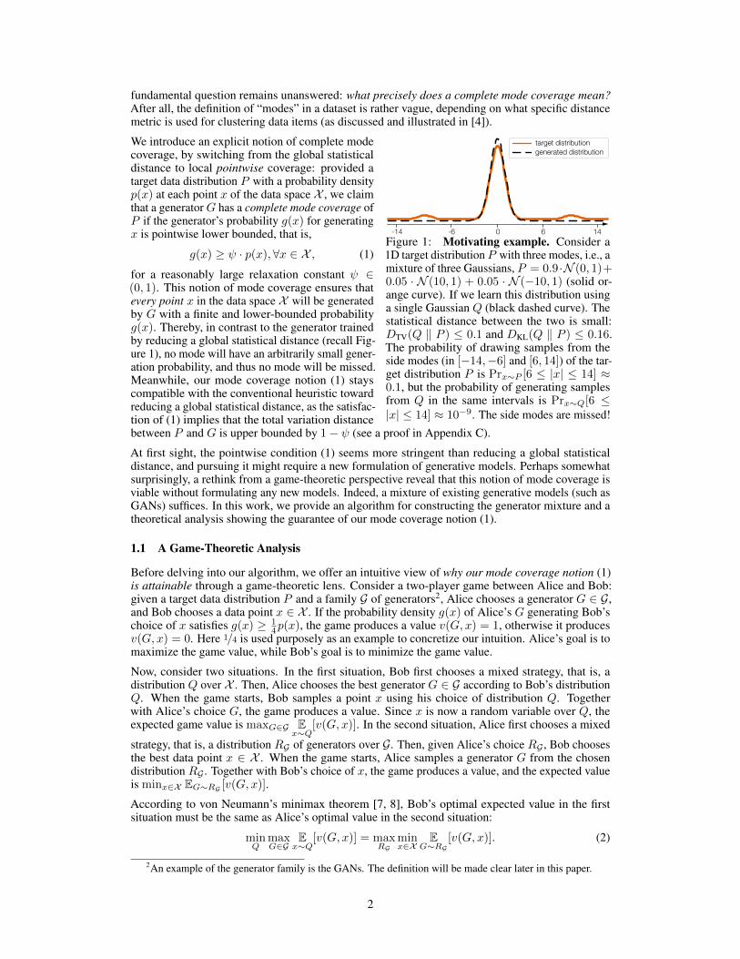
0 6 14-6-14Figure 1: Motivating example. Consider a1D target distribution P with three modes, i.e., amixture of three Gaussians, P = 0.9 ·N (0, 1)+0.05 · N (10, 1) + 0.05 · N (−10, 1) (solid or-ange curve). If we learn this distribution usinga single Gaussian Q (black dashed curve). Thestatistical distance between the two is small:DTV(Q ‖ P ) ≤ 0.1 and DKL(Q ‖ P ) ≤ 0.16.The probability of drawing samples from theside modes (in [−14,−6] and [6, 14]) of the tar-get distribution P is Prx∼P [6 ≤ |x| ≤ 14] ≈0.1, but the probability of generating samplesfrom Q in the same intervals is Prx∼Q[6 ≤|x| ≤ 14] ≈ 10−9. The side modes are missed!

We introduce an explicit notion of complete modecoverage, by switching from the global statisticaldistance to local pointwise coverage: provided atarget data distribution P with a probability densityp(x) at each point x of the data space X , we claimthat a generatorG has a complete mode coverage ofP if the generator’s probability g(x) for generatingx is pointwise lower bounded, that is,

g(x) ≥ ψ · p(x),∀x ∈ X , (1)

for a reasonably large relaxation constant ψ ∈(0, 1). This notion of mode coverage ensures thatevery point x in the data space X will be generatedby G with a finite and lower-bounded probabilityg(x). Thereby, in contrast to the generator trainedby reducing a global statistical distance (recall Fig-ure 1), no mode will have an arbitrarily small gener-ation probability, and thus no mode will be missed.Meanwhile, our mode coverage notion (1) stayscompatible with the conventional heuristic towardreducing a global statistical distance, as the satisfac-tion of (1) implies that the total variation distancebetween P and G is upper bounded by 1− ψ (see a proof in Appendix C).

At first sight, the pointwise condition (1) seems more stringent than reducing a global statisticaldistance, and pursuing it might require a new formulation of generative models. Perhaps somewhatsurprisingly, a rethink from a game-theoretic perspective reveal that this notion of mode coverage isviable without formulating any new models. Indeed, a mixture of existing generative models (such asGANs) suffices. In this work, we provide an algorithm for constructing the generator mixture and atheoretical analysis showing the guarantee of our mode coverage notion (1).

1.1 A Game-Theoretic Analysis

Before delving into our algorithm, we offer an intuitive view of why our mode coverage notion (1)is attainable through a game-theoretic lens. Consider a two-player game between Alice and Bob:given a target data distribution P and a family G of generators2, Alice chooses a generator G ∈ G,and Bob chooses a data point x ∈ X . If the probability density g(x) of Alice’s G generating Bob’schoice of x satisfies g(x) ≥ 1

4p(x), the game produces a value v(G, x) = 1, otherwise it producesv(G, x) = 0. Here 1/4 is used purposely as an example to concretize our intuition. Alice’s goal is tomaximize the game value, while Bob’s goal is to minimize the game value.

Now, consider two situations. In the first situation, Bob first chooses a mixed strategy, that is, adistribution Q over X . Then, Alice chooses the best generator G ∈ G according to Bob’s distributionQ. When the game starts, Bob samples a point x using his choice of distribution Q. Togetherwith Alice’s choice G, the game produces a value. Since x is now a random variable over Q, theexpected game value is maxG∈G E

x∼Q[v(G, x)]. In the second situation, Alice first chooses a mixed

strategy, that is, a distribution RG of generators over G. Then, given Alice’s choice RG , Bob choosesthe best data point x ∈ X . When the game starts, Alice samples a generator G from the chosendistribution RG . Together with Bob’s choice of x, the game produces a value, and the expected valueis minx∈X EG∼RG [v(G, x)].

According to von Neumann’s minimax theorem [7, 8], Bob’s optimal expected value in the firstsituation must be the same as Alice’s optimal value in the second situation:

minQ

maxG∈G

Ex∼Q

[v(G, x)] = maxRG

minx∈X

EG∼RG

[v(G, x)]. (2)

2An example of the generator family is the GANs. The definition will be made clear later in this paper.

2

With this equality realized, our agenda in the rest of the analysis is as follows. First, we show a lowerbound of the left-hand side of (2), and then we use the right-hand side to reach the lower-boundof g(x) as in (1), for Alice’s generator G. To this end, we need to depart off from the currentgame-theoretic analysis and discuss the properties of existing generative models for a moment.

Existing generative models such as GANs [9, 1, 10] aim to reproduce arbitrary data distributions.While it remains intractable to have the generated distribution match exactly the data distribution,the approximations are often plausible. One reason behind the plausible performance is that the dataspace encountered in practice is “natural” and restricted—all English sentences or all natural objectimages or all images on a manifold—but not a space of arbitrary data. Therefore, it is reasonable toexpect the generators in G (e.g., all GANs) to meet the following requirement3 (without conflictingthe no-free-lunch theorem [11]): for any distribution Q over a natural data space X encounteredin practice, there exists a generator G ∈ G such that the total variation distance between G and Qis upper bounded by a constant γ, that is, 1

2

∫X |q(x)− g(x)|dx ≤ γ, where q(·) and g(·) are the

probability densities on Q and the generated samples of G, respectively. Again as a concrete example,we use γ = 0.1. With this property in mind, we now go back to our game-theoretic analysis.

Back to the first situation described above. Once Bob’s distribution Q (over X ) and Alice’s generatorG are identified, then given a target distribution P over X and an x drawn by Bob from Q, theprobability of having Alice’s G cover P (i.e., g(x) ≥ 1

4p(x)) at x is lower bounded. In our currentexample, we have the following lower bound:

Prx∼Q

[g(x) ≥ 1/4 · p(x)] ≥ 0.4. (3)

Here 0.4 is related to the total variation distance bound (i.e., γ = 0.1) between G and Q, and thislower bound value is derived in Appendix D. Next, notice that on the left-hand side of (2), theexpected value, Ex∼Q[v(G, x)], is equivalent to the probability in (3). Thus, we have

minQ

maxG∈G

Ex∼Q

[v(G, x)] ≥ 0.4. (4)

Because of the equality in (2), this is also the lower bound of its right-hand side, from which we knowthat there exists a distribution RG of generators such that for any x ∈ X , we have

EG∼RG

[v(G, x)] = PrG∼RG

[g(x) ≥ 1/4 · p(x)] ≥ 0.4. (5)

This expression shows that for any x ∈ X , if we draw a generator G from RG , then with a probabilityat least 0.4, G’s generation probability density satisfies g(x) ≥ 1

4p(x). Thus, we can think RG as a“collective” generator G∗, or a mixture of generators. When generating a sample x, we first choosea generator G according to RG and then sample an x using G. The overall probability g∗(x) ofgenerating x satisfies g∗(x) > 0.1p(x)—precisely the pointwise lower bound that we pose in (1).

Takeaway from the analysis. This analysis reveals that a complete mode coverage is firmly viable.Yet it offers no recipe on how to construct the mixture of generators and their distribution RG usingexisting generative models. Interestingly, as pointed out by Arora et al. [12], a constructive versionof von Neumann’s minimax theorem is related to the general idea of multiplicative weights update.Therefore, our key contributions in this work are i) the design of a multiplicative weights updatealgorithm (in Sec. 3) to construct a generator mixture, and ii) a theoretical analysis showing thatour generator mixture indeed obtains the pointwise data coverage (1). In fact, we only need a smallnumber of generators to construct the mixture (i.e., it is easy to train), and the distribution RG forusing the mixture is as simple as a uniform distribution (i.e., it is easy to use).

2 Related Work

There exists a rich set of works improving classic generative models for alleviating missing modes,especially in the framework of GANs, by altering objective functions [13, 14, 15, 10, 16, 17],changing training methods [18, 19], modifying neural network architectures [2, 20, 21, 22, 23], orregularizing latent space distributions [4, 24]. The general philosophy behind these improvements isto reduce the statistical distance between the generated distribution and target distribution by making

3This requirement is weaker than the mainstream goal of generative models, which all aim to approximate atarget data distribution as closely as possible. Here we only require the approximation error is upper bounded.

3

the models easier to train. Despite their technical differences, their optimization goals are all towardreducing a global statistical distance.

The idea of constructing a mixture of generators has been explored, with two ways of construction.In the first way, a set of generators are trained simultaneously. For example, Locatello et al. [25]used multiple generators, each responsible for sampling a subset of data points decided in a k-meansclustering fashion. Other methods focus on the use of multiple GANs [26, 27, 28]. The theoreticalintuition behind these approaches is by viewing a GAN as a two-player game and extending it toreach a Nash equilibrium with a mixture of generators [26]. In contrast, our method does not dependspecifically on GANs, and our game-theoretic view is fundamentally different (recall Sec. 1.1).

Another way of training a mixture of generators takes a sequential approach. This is related to boostingalgorithms in machine learning. Grnarova et al. [29] viewed the problem of training GANs as findinga mixed strategy in a zero-sum game, and used the Follow-the-Regularized-Leader algorithm [30]for training a mixture of generators iteratively. Inspired by AdaBoost [31], other approaches train a“weak” generator that fits a reweighted data distribution in each iteration, and all iterations togetherform an additive mixture of generators [32, 33] or a multiplicative mixture of generators [34].

Our method can be also viewed as a boosting strategy. From this perspective, the most related isAdaGAN [33], while significant differences exist. Theoretically, AdaGAN (and other boosting-likealgorithms) is based on the assumption that the reweighted data distribution in each iteration becomesprogressively easier to learn. It requires a generator in each iteration to have a statistical distanceto the reweighted distribution smaller than the previous iteration. As we will discuss in Sec. 5,this assumption is not always feasible. We have no such assumption. Our method can use a weakgenerator in each iteration. If the generator is more expressive, the theoretical lower bound of ourpointwise coverage becomes larger (i.e., a larger ψ in (1)). Algorithmically, our reweighting schemeis simple and different from AdaGAN, only doubling the weights or leaving them unchanged in eachiteration. Also, in our mixture of generators, they are treated uniformly, and no mixture weights areneeded, whereas AdaGAN needs a set of weights that are heuristically chosen.

To summarize, in stark contrast to all prior methods, our approach is rooted in a different philosophyof training generative models. Rather than striving for reducing a global statistical distance, ourmethod revolves around an explicit notion of complete mode coverage as defined in (1). Unlike otherboosting algorithms, our algorithm of constructing the mixture of generators guarantees completemode coverage, and this guarantee is theoretically proved.

3 Algorithm

A mixture of generators. Provided a target distribution P on a data domain X , we train a mixtureof generators to pursue pointwise mode coverage (1). Let G∗ = G1, . . . , GT denote the resultingmixture of T generators. Each of them (Gt, t = 1...T ) may use any existing generative model suchas GANs. Existing methods that also rely on a mixture of generators associate each generator anonuniform weight αt and choose a generator for producing a sample randomly based on the weights.Often, these weights are chosen heuristically, e.g., in AdaGAN [33]. Our mixture is conceptually andcomputationally simpler. Each generator is treated equally. When using G∗ to generate a sample, wefirst choose a generator Gi uniformly at random, and then use Gi to generate the sample.

Algorithm overview. Our algorithm of training G∗ can be understood as a specific rule design inthe framework of multiplicative weights update [12]. Outlined in Algorithm 1, it runs iteratively.In each iteration, a generator Gt is trained using an updated data distribution Pt (see Line 6-7 ofAlgorithm 1). The intuition here is simple: if in certain data domain regions the current generator failsto cover the target distribution sufficiently well, then we update the data distribution to emphasizethose regions for the next round of generator training (see Line 9 of Algorithm 1). In this way, eachgenerator can focus on the data distribution in individual data regions. Collectively, they are able tocover the distribution over the entire data domain, and thus guarantee pointwise data coverage.

Training. Each iteration of our algorithm trains an individual generatorGt, for which many existinggenerative models, such as GANs [9], can be used. The only prerequisite is that Gt needs to betrained to approximate the data distribution Pt moderately well. This requirement arises from ourgame-theoretic analysis (Sec. 1.1), wherein the total variation distance between Gt’s distribution andPt needs to be upper bounded. Later in our theoretical analysis (Sec. 4), we will formally state thisrequirement, which, in practice, is easily satisfied by most existing generative models.

4

Algorithm 1 Constructing a mixture of generators1: Parameters: T , a positive integer number of generators, and δ ∈ (0, 1), a covering threshold.2: Input: a target distribution P on a data domain X .3: For each x ∈ X , initialize its weight w1(x) = p(x).4: for t = 1→ T do5: Construct a distribution Pt over X as follows:6: For every x ∈ X , normalize the probability density pt(x) = wt(x)

Wt, where Wt =

∫X wt(x)dx.

7: Train a generative model Gt on the distribution Pt.8: Estimate generated density gt(x) for every x ∈ X .9: For each x ∈ X , if gt(x) < δ ·p(x), setwt+1(x) = 2·wt(x). Otherwise, setwt+1(x) = wt(x).

10: end for11: Output: a mixture of generators G∗ = G1, . . . , GT .

Estimation of generated probability density. In Line 8 of Algorithm 1, we need to estimate theprobability gt(x) of the current generator sampling a data point x. Our estimation follows the ideaof adversarial training, similar to AdaGAN [33]. First, we train a discriminator Dt to distinguishbetween samples from Pt and samples from Gt. The optimization objective of Dt is defined as

maxDt

Ex∼Pt

[logDt(x)] + Ex∼Gt

[log(1−Dt(x))].

Unlike AdaGAN [33], here Pt is the currently updated data distribution, not the original targetdistribution, and Gt is the generator trained in the current round, not a mixture of generators in allpast rounds. As pointed out previously [35, 33], once Dt is optimized, we have Dt(x) = pt(x)

pt(x)+gt(x)

for all x ∈ X , and equivalently gt(x)pt(x) = 1

Dt(x) − 1. Using this property in Line 9 of Algorithm 1 (fortesting the data coverage), we rewrite the condition gt(x) < δ · p(x) as

gt(x)

p(x)=gt(x)

pt(x)

pt(x)

p(x)=

(1

Dt(x)− 1

)wt(x)

p(x)Wt< δ,

where the second equality utilize the evaluation of pt(x) in Line 6 (i.e., pt(x) = wt(x)/Wt).

Note that if the generators Gt are GANs, then the discriminator of each Gt can be reused as Dt here.Reusing Dt introduces no additional computation. In contrast, AdaGAN [33] always has to train anadditional discriminator Dt in each round using the mixture of generators of all past rounds.

Working with empirical dataset. In practice, the true data distribution P is often unknown whenan empirical dataset X = xini=1 is given. Instead, the empirical dataset is considered as n i.i.d.samples drawn from P . According to the Glivenko-Cantelli theorem [36], the uniform distributionover n i.i.d. samples from P will converge to P as n approaches to infinity. Therefore, provided theempirical dataset, we do not need to know the probability density p(x) of P , as every sample xi ∈ Xis considered to have a finite and uniform probability measure. An empirical version of Algorithm 1and more explanation are presented in the supplementary document (Algorithm 2 and Appendix B).

4 Theoretical Analysis

We now provide a theoretical understanding of our algorithm, showing that the pointwise datacoverage (1) is indeed obtained. Our analysis also sheds some light on how to choose the parametersof Algorithm 1.

4.1 Preliminaries

We first clarify a few notational conventions and introduce two new theoretical notions for oursubsequent analysis. Our analysis is in continuous setting; results on discrete datasets follow directly.

Notation. Formally, we consider a d-dimensional measurable space (X ,B(X )), where X is thed-dimensional data space, and B(X ) is the Borel σ-algebra over X to enable probability measure. Weuse a capital letter (e.g., P ) to denote a probability measure on this space. When there is no ambiguity,we also refer them as probability distributions (or distributions). For any subset S ∈ B(X ), theprobability of S under P is P (S) := Prx∼P [x ∈ S]. We use G to denote a generator. When there is

5

no ambiguity, G also denotes the distribution of its generated samples. All distributions are assumedabsolutely continuous. Their probability density functions (i.e., the derivative with respect to theLebesgue measure) are referred by their corresponding lowercase letters (e.g., p(·), q(·), and g(·)).

Moreover, we use [n] to denote the set 1, 2, ..., n, N>0 for the set of all positive integers, and 1(E)for the indicator function whose value is 1 if the event E happens, and 0 otherwise.

f -divergence. Widely used in objective functions of training generative models, f -divergence is astatistical distance between two distributions. Let P and Q be two distributions over X . Provided aconvex function f on (0,∞) such that f(1) = 0, f -divergence of Q from P is defined as Df (Q ‖P ) :=

∫X f

(q(x)p(x)

)p(x)dx. Various choices of f lead to some commonly used f -divergence metrics

such as total variation distance DTV, Kullback-Leibler divergence DKL, Hellinger distance DH, andJensen-Shannon divergence DJS [35, 37]. Among them, total variation distance is upper bounded

by many other f -divergences. For instance, DTV(Q ‖ P ) is upper bounded by√

12DKL(Q ‖ P ),

√2DH(Q ‖ P ), and

√2DJS(Q ‖ P ), respectively. Thus, if two distributions are close under those

f -divergence measures, so are they under total variation distance. For this reason, our theoreticalanalysis is based on the total variation distance.

δ-cover and (δ, β)-cover. We introduce two new notions for analyzing our algorithm. The first isthe notion of δ-cover. Given a data distribution P over X and a value δ ∈ (0, 1], if a generator Gsatisfies g(x) ≥ δ · p(x) at a data point x ∈ X , we say that x is δ-covered by G under distribution P .Using this notion, the pointwise mode coverage (1) states that x is ψ-covered by G under distributionP for all x ∈ X . We also extend this notion to a measurable subset S ∈ B(X ): we say that S isδ-covered by G under distribution P if G(S) ≥ δ · P (S) is satisfied.

Next, consider another distribution Q over X . We say that G can (δ, β)-cover (P,Q), if the followingcondition holds:

Prx∼Q

[x is δ-covered by G under distributionP ] ≥ β. (6)

For instance, using this notation, Equation (3) in our game-theoretic analysis states that G can(0.25, 0.4)-cover (P,Q).

4.2 Guarantee of Pointwise Data Coverage

In each iteration of Algorithm 1, we expect the generatorGt to approximate the given data distributionPt sufficiently well. We now formalize this expectation and understand its implication. Our intuitionis that by finding a property similar to (3), we should be able to establish a pointwise coverage lowerbound in a way similar to our analysis in Sec. 1.1. Such a property is given by the following lemma(and proved in Appendix E.1).Lemma 1. Consider two distributions, P andQ, over the data spaceX , and a generatorG producingsamples in X . For any δ, γ ∈ (0, 1], if DTV (G ‖ Q) ≤ γ, then G can (δ, 1− 2δ − γ)-cover (P,Q).

Intuitively, when G and Q are identified, γ is set. If δ is reduced, then more data points in X canbe δ-covered by G under P . Thus, the probability defined in (6) becomes larger, as reflected by theincreasing 1− 2δ − γ. On the other hand, consider a fixed δ. As the discrepancy between G and Qbecomes larger, γ increases. Then, sampling an x according to Q will have a smaller chance to landat a point that is δ-covered by G under P , as reflected by the decreasing 1− 2δ − γ.

Next, we consider Algorithm 1 and identify a sufficient condition under which the output mixture ofgenerators G∗ covers every data point with a lower-bounded guarantee (i.e., our goal (1)). Simplyspeaking, this sufficient condition is as follows: in each round t, the generator Gt is trained such thatgiven an x drawn from distribution Pt, the probability of x being δ-covered by Gt under P is alsolower bounded. A formal statement is given in the next lemma (proved in Appendix E.2).Lemma 2. Recall that T ∈ N>0 and δ ∈ (0, 1) are the input parameters of Algorithm 1. For anyε ∈ [0, 1) and any measurable subset S ∈ B(X ) whose probability measure satisfies P (S) ≥ 1/2ηT

with some η ∈ (0, 1), if in every round t ∈ [T ], Gt can (δ, 1− ε)-cover (P, Pt), then the resultingmixture of generators G∗ can (1− ε/ln 2− η)δ-cover S under distribution P .

This lemma is about lower-bounded coverage of a measurable subset S, not a point x ∈ X . At firstsight, it is not of the exact form in (1) (i.e., pointwise δ-coverage). This is because formally speakingit makes no sense to talk about covering probability at a single point (whose measure is zero). But as

6

T approaches to∞, S that satisfies P (S) ≥ 1/2ηT can also approach to a point (and η approachesto zero). Thus, Lemma 2 provides a condition for pointwise lower-bounded coverage in the limitingsense. In practice, the provided dataset is always discrete, and the probability measure at each discretedata point is finite. Then, Lemma 2 is indeed a sufficient condition for pointwise lower-boundedcoverage.

From Lemma 1, we see that the condition posed by Lemma 2 is indeed satisfied by our algorithm,and combing both lemmas yields our final theorem (proved in Appendix E.3).Theorem 1. Recall that T ∈ N>0 and δ ∈ (0, 1) are the input parameters of Algorithm 1. Forany measurable subset S ∈ B(X ) whose probability measure satisfies P (S) ≥ 1/2ηT with someη ∈ (0, 1), if in every round t ∈ [T ], DTV(Gt ‖ Pt) ≤ γ, then the resulting mixture of generators G∗can (1− (γ + 2δ)/ ln 2− η)δ-cover S under distribution P .In practice, existing generative models (such as GANs) can approximate Pt sufficiently well, andthus DTV(Gt ‖ Pt) ≤ γ is always satisfied for some γ. According to Theorem 1, a pointwiselower-bounded coverage can be obtained by our Algorithm 1. If we choose to use a more expressivegenerative model (e.g., a GAN with a stronger network architecture), then Gt can better fit Pt in eachround, yielding a smaller γ used in Theorem 1. Consequently, the pointwise lower bound of the datacoverage becomes larger, and effectively the coefficient ψ in (1) becomes larger.

4.3 Insights from the Analysis

γ, η, δ, and T in Theorem 1. In Theorem 1, γ depends on the expressive power of the generatorsbeing used. It is therefore determined once the generator class G is chosen. But η can be directly setby the user and a smaller η demands a larger T to ensure P (S) ≥ 1/2ηT is satisfied. Once γ and η isdetermined, we can choose the best δ by maximizing the coverage bound (i.e., (1−(γ+2δ)/ ln 2−η)δ)in Theorem 1. For example, if γ ≤ 0.1, η ≤ 0.01, then δ ≈ 1/4 would optimize the coverage bound(see Appendix E.4 for more details), and in this case the coefficient ψ in (1) is at least 1/30.

Theorem 1 also sets the tone for the training cost. As explained in Appendix E.4, given a trainingdataset of size n, the size of the generator mixture, T , needs to be at most O(log n). This theoreticalbound is consistent with our experimental results presented in Sec. 5. In practice, only a small numberof generators are needed.Estimated density function gt. The analysis in Sec. 4.2 assumes that the generated probabilitydensity gt of the generator Gt in each round is known, while in practice we have to estimate gt bytraining a discriminator Dt (recall Section 3). Fortunately, only mild assumptions in terms of thequality of Dt are needed to retain the pointwise lower-bounded coverage. Roughly speaking, Dt

needs to meet two conditions: 1) In each round t, only a fraction of the covered data points (i.e., thosewith gt(x) ≥ δ · p(x)) is falsely classified by Dt and doubled their weights. 2) In each round t, if theweight of a data point x is not doubled based on the estimation of Dt(x), then there is a good chancethat x is truly covered by Gt (i.e., gt(x) ≥ δ · p(x)). A detailed and formal discussion is presented inAppendix E.5. In short, our estimation of gt would not deteriorate the efficacy of the algorithm, asalso confirmed in our experiments.Generalization. An intriguing question for all generative models is their generalization perfor-mance: how well can a generator trained on an empirical distribution (with a finite number ofdata samples) generate samples that follow the true data distribution? While the generalizationperformance has been long studied for supervised classification, generalization of generative modelsremains a widely open theoretical question. We propose a notion of generalization for our method,and provide a preliminary theoretical analysis. All the details are presented in Appendix E.6.

5 ExperimentsWe now present our major experimental results, while referring to Appendix F for network detailsand more results. We show that our mixture of generators is able to cover all the modes in varioussynthetic and real datasets, while existing methods always have some modes missed.Previous works on generative models used the Inception Score [1] or the Fréchet Inception Dis-tance [18] as their evaluation metric. But we do not use them, because they are both global measures,not reflecting mode coverage in local regions [38]. Moreover, these metrics are designed to measurethe quality of generated images, which is orthogonal to our goal. For example, one can always use amore expressive GAN in each iteration of our algorithm to obtain better image quality and thus betterinception scores.

7

(a) (b) (c) (d) (e) (f)

Figure 2: Generative models on synthetic dataset. (a) The dataset consists of two modes: onemajor mode as an expanding sine curve (y = x sin 4x

π ) and a minor mode as a Gaussian located at(10, 0) (highlighted in the reb box). (b-f) We show color-coded distributions of generated samplesfrom (b) EM, (c) GAN, (d) VAE, (e) AdaGAN, and (f) our method (i.e., a mixture of GANs). Onlyour method is able to cover the second mode (highlighted in the green box; zoomin to view).

Since the phenomenon of missing modes is particularly prominent in GANs, our experimentsemphasize on the mode coverage performance of GANs and compare our method (using a mixture ofGANs) with DCGAN [39], MGAN [27], and AdaGAN. The latter two also use multiple GANs toimprove mode coverage, although they do not aim for the same mode coverage notion as ours.

Overview. We first outline all our experiments, including those presented in Appendix F. i) Wecompare our method with a number of classic generative models on a synthetic dataset. ii) InAppendix F.3, we also compare our method with AdaGAN [33] on other synthetic datasets as well asstacked MNIST dataset, because both are boosting algorithms aiming at improving mode coverage.iii) We further compare our method with a single large DCGAN, AdaGAN, and MGAN on theFashion-MNIST dataset [40] mixed with a very small portion of MNIST dataset [41].

Various generative models on synthetic dataset. As we show in Appendix A, many generativemodels, such as expectation-maximization (EM) methods, VAEs, and GANs, all rely on a globalstatistical distance in their training. We therefore test their mode coverage and compare with ours.We construct on R2 a synthetic dataset with two modes. The first mode consists of data points whosex-coordinate is uniformly sampled by xi ∼ [−10, 10] and the y-coordinate is yi = xi sin 4xi

π . Thesecond mode has data points forming a Gaussian at (0, 10). The total number of data points in thefirst mode is 400× of the second. As shown in Figure 2, generative models include EM, GAN, VAE,and AdaGAN [33] all fail to cover the second mode. Our method, in contrast, captures both modes.We run KDE to estimate the likelihood of our generated samples on our synthetic data experiments(using KDE bandwidth=0.1). We compute L = 1/N

∑i Pmodel(xi), where xi is a sample in the

minor mode. For the minor mode, our method has a mean log likelihood of -1.28, while AdaGANhas only -967.64 (almost no samples from AdaGAN).

“1”s Frequency Avg Prob.DCGAN 13 0.14× 10−4 0.49MGAN collapsed - -AdaGAN 60 0.67× 10−4 0.45Our method 289 3.2× 10−4 0.68

Table 1: Ratios of generated images classified as“1”. We generate 9× 105 images from each method.The second column indicates the numbers of sam-ples being classified as “1”, and the third columnindicates the ratio. In the fourth column, we averagethe prediction probabilities over all generated imagesthat are classified as “1”.

Fashion-MNIST and partial MNIST. Ournext experiment is to challenge different GANmodels with a real dataset that has separatedand unbalanced modes. This dataset con-sists of the entire training dataset of Fashion-MNIST (with 60k images) mixed with ran-domly sampled 100 MNIST images labeledas “1”. The size of generator mixture is al-ways set to be 30 for AdaGAN, MGAN andour method, and all generators share the samenetwork structure. Additionally, when com-paring with a single DCGAN, we ensure thatthe DCGAN’s total number of parameters iscomparable to the total number of parameters of the 30 generators in AdaGAN, MGAN, and ours.To evaluate the results, we train an 11-class classifier to distinguish the 10 classes in Fashion-MNISTand one class in MNIST (i.e., “1”). First, we check how many samples from each method areclassified as “1”. The test setup and results are shown in Table 1 and its caption. The results suggestthat our method can generate more “1” samples with higher prediction confidence. Note that MGANhas a strong mode collapse and fails to produce “1” samples. While DCGAN and AdaGAN generatesome samples that are classified as “1”, inspecting the generated images reveals that those samplesare all visually far from “1”s, but incorrectly classified by the pre-trained classifier (see Figure 3).In contrast, our method is able to generate samples close to “1”. We also note that our method canproduce higher-quality images if the underlying generative models in each round become stronger.

8

AdaGAN MGAN DCGAN Our ApproachFigure 3: Most confident “1” samples. Here we show samples that are generated by each testedmethods and also classified by the pre-trained classifier most confidently as “1” images (i.e., top 10in terms of the classified probability). Samples of our method are visually much closer to “1”.

0.6

0.5

0.40.3

0.20.1

0.00 1 2 3 4 5 6 7 8 9

0.6

0.5

0.40.3

0.20.1

0.00 1 2 3 4 5 6 7 8 9

0.6

0.5

0.40.3

0.20.1

0.00 1 2 3 4 5 6 7 8 9

0.6

0.5

0.40.3

0.20.1

0.00 1 2 3 4 5 6 7 8 9

AdaGAN MGAN DCGAN OursClass

Frequency Frequency Frequency Frequency

Class Class Class

Figure 5: Distribution of generated samples. Training samples are drawn uniformly from eachclass. But generated samples by AdaGAN and MGAN are considerably nonuniform, while thosefrom DCGAN and our method are more uniform. This experiment suggests that the conventionalheuristic of reducing a statistical distance might not merit its use in training generative models.

0.005

0.00160 10 20 30 40 50

Ratio

Iterations

Figure 4: Weight ratio of “1”s. We calculatethe ratio of the total weights of training imageslabeled by “1” to the total weights of all trainingimages in each round, and plot here how theratio changes with respect to the iterations inour algorithm.

Another remarkable feature is observed in ouralgorithm. In each round of our training algorithm,we calculate the total weight wt of provided train-ing samples classified as “1” as well as the totalweight Wt of all training samples. When plottingthe ratio wt/Wt changing with respect to the num-ber of rounds (Figure 4), interestingly, we foundthat this ratio has a maximum value at around 0.005in this example. We conjecture that in the trainingdataset if the ratio of “1” images among all trainingimages is around 1/200, then a single generatormay learn and generate “1” images (the minoritymode). To verify this conjecture, we trained a GAN (with the same network structure) on anothertraining dataset with 60k training images from Fashion-MNIST mixed with 300 MNIST “1” images.We then use the trained generator to sample 100k images. As a result, In a fraction of 4.2× 10−4,those images are classified as “1”. Figure 8 in Appendix F shows some of those images. This resultconfirms our conjecture and suggests that wt/Wt may be used as a measure of mode bias in a dataset.

Lastly, in Figure 5, we show the generated distribution over the 10 Fashion-MNIST classes fromeach tested method. We neglect the class “1”, as MGAN fails to generate them. The generatedsamples of AdaGAN and MGAN is highly nonuniform, though in the training dataset, the 10 classesof images are uniformly distributed. Our method and DCGAN produce more uniform samples. Thissuggests that although other generative models (such as AdaGAN and MGAN) aim to reduce a globalstatistical distance, the generated samples may not easily match the empirical distribution—in thiscase, a uniform distribution. Our method, while not aiming for reducing the statistical distance in thefirst place, matches the target empirical distribution plausibly, as a byproduct.

6 Conclusion

We have presented an algorithm that iteratively trains a mixture of generators, driven by an explicitnotion of complete mode coverage. With this notion for designing generative models, our work posesan alternative goal, one that differs from the conventional training philosophy: instead of reducing aglobal statistical distance between the target distribution and generated distribution, one only needsto make the distance mildly small but not have to reduce it toward a perfect zero, and our method isable to boost the generative model with theoretically guaranteed mode coverage.

Acknowledgments. This work was supported in part by the National Science Foundation (CAREER-1453101, 1816041, 1910839, 1703925, 1421161, 1714818, 1617955, 1740833), SimonsFoundation (#491119 to Alexandr Andoni), Google Research Award, a Google PhD Fellowship, aSnap Research Fellowship, a Columbia SEAS CKGSB Fellowship, and SoftBank Group.

9

References[1] Tim Salimans, Ian Goodfellow, Wojciech Zaremba, Vicki Cheung, Alec Radford, and Xi Chen.

Improved techniques for training gans. In Advances in Neural Information Processing Systems,pages 2234–2242, 2016.

[2] Luke Metz, Ben Poole, David Pfau, and Jascha Sohl-Dickstein. Unrolled generative adversarialnetworks. arXiv preprint arXiv:1611.02163, 2016.

[3] Nitish Srivastava, Geoffrey Hinton, Alex Krizhevsky, Ilya Sutskever, and Ruslan Salakhutdinov.Dropout: A simple way to prevent neural networks from overfitting. The Journal of MachineLearning Research, 15(1):1929–1958, 2014.

[4] Chang Xiao, Peilin Zhong, and Changxi Zheng. Bourgan: Generative networks with metricembeddings. In Advances in Neural Information Processing Systems, pages 2269–2280, 2018.

[5] Xi Chen, Yan Duan, Rein Houthooft, John Schulman, Ilya Sutskever, and Pieter Abbeel. Infogan:Interpretable representation learning by information maximizing generative adversarial nets. InAdvances in Neural Information Processing Systems, pages 2172–2180, 2016.

[6] Samuel R Bowman, Luke Vilnis, Oriol Vinyals, Andrew Dai, Rafal Jozefowicz, and SamyBengio. Generating sentences from a continuous space. In Proceedings of The 20th SIGNLLConference on Computational Natural Language Learning, pages 10–21, 2016.

[7] J v Neumann. Zur theorie der gesellschaftsspiele. Mathematische annalen, 100(1):295–320,1928.

[8] Ding-Zhu Du and Panos M Pardalos. Minimax and applications, volume 4. Springer Science &Business Media, 2013.

[9] Ian Goodfellow, Jean Pouget-Abadie, Mehdi Mirza, Bing Xu, David Warde-Farley, SherjilOzair, Aaron Courville, and Yoshua Bengio. Generative adversarial nets. In Advances in neuralinformation processing systems, pages 2672–2680, 2014.

[10] Martin Arjovsky, Soumith Chintala, and Léon Bottou. Wasserstein gan. arXiv preprintarXiv:1701.07875, 2017.

[11] David H Wolpert, William G Macready, et al. No free lunch theorems for optimization. IEEEtransactions on evolutionary computation, 1(1):67–82, 1997.

[12] Sanjeev Arora, Elad Hazan, and Satyen Kale. The multiplicative weights update method: ameta-algorithm and applications. Theory of Computing, 8(1):121–164, 2012.

[13] Tong Che, Yanran Li, Athul Paul Jacob, Yoshua Bengio, and Wenjie Li. Mode regularizedgenerative adversarial networks. arXiv preprint arXiv:1612.02136, 2016.

[14] Junbo Zhao, Michael Mathieu, and Yann LeCun. Energy-based generative adversarial network.arXiv preprint arXiv:1609.03126, 2016.

[15] Xudong Mao, Qing Li, Haoran Xie, Raymond YK Lau, Zhen Wang, and Stephen Paul Smolley.Least squares generative adversarial networks. In 2017 IEEE International Conference onComputer Vision (ICCV), pages 2813–2821. IEEE, 2017.

[16] Ishaan Gulrajani, Faruk Ahmed, Martin Arjovsky, Vincent Dumoulin, and Aaron C Courville.Improved training of wasserstein gans. In Advances in Neural Information Processing Systems,pages 5769–5779, 2017.

[17] Yunus Saatci and Andrew G Wilson. Bayesian gan. In Advances in neural informationprocessing systems, pages 3622–3631, 2017.

[18] Martin Heusel, Hubert Ramsauer, Thomas Unterthiner, Bernhard Nessler, and Sepp Hochreiter.Gans trained by a two time-scale update rule converge to a local nash equilibrium. In Advancesin Neural Information Processing Systems, pages 6626–6637, 2017.

10

[19] Andrew Brock, Jeff Donahue, and Karen Simonyan. Large scale gan training for high fidelitynatural image synthesis. arXiv preprint arXiv:1809.11096, 2018.

[20] Vincent Dumoulin, Ishmael Belghazi, Ben Poole, Olivier Mastropietro, Alex Lamb, Martin Ar-jovsky, and Aaron Courville. Adversarially learned inference. arXiv preprint arXiv:1606.00704,2016.

[21] Zinan Lin, Ashish Khetan, Giulia Fanti, and Sewoong Oh. Pacgan: The power of two samplesin generative adversarial networks. arXiv preprint arXiv:1712.04086, 2017.

[22] Akash Srivastava, Lazar Valkoz, Chris Russell, Michael U Gutmann, and Charles Sutton.Veegan: Reducing mode collapse in gans using implicit variational learning. In Advances inNeural Information Processing Systems, pages 3310–3320, 2017.

[23] Tero Karras, Timo Aila, Samuli Laine, and Jaakko Lehtinen. Progressive growing of gans forimproved quality, stability, and variation. arXiv preprint arXiv:1710.10196, 2017.

[24] Chongxuan Li, Max Welling, Jun Zhu, and Bo Zhang. Graphical generative adversarial networks.In S. Bengio, H. Wallach, H. Larochelle, K. Grauman, N. Cesa-Bianchi, and R. Garnett, editors,Advances in Neural Information Processing Systems 31, pages 6072–6083. Curran Associates,Inc., 2018.

[25] Francesco Locatello, Damien Vincent, Ilya Tolstikhin, Gunnar Rätsch, Sylvain Gelly, and Bern-hard Schölkopf. Clustering meets implicit generative models. arXiv preprint arXiv:1804.11130,2018.

[26] Sanjeev Arora, Rong Ge, Yingyu Liang, Tengyu Ma, and Yi Zhang. Generalization andequilibrium in generative adversarial nets (gans). arXiv preprint arXiv:1703.00573, 2017.

[27] Quan Hoang, Tu Dinh Nguyen, Trung Le, and Dinh Phung. MGAN: Training generative adver-sarial nets with multiple generators. In International Conference on Learning Representations,2018.

[28] David Keetae Park, Seungjoo Yoo, Hyojin Bahng, Jaegul Choo, and Noseong Park. Megan:Mixture of experts of generative adversarial networks for multimodal image generation. arXivpreprint arXiv:1805.02481, 2018.

[29] Paulina Grnarova, Kfir Y Levy, Aurelien Lucchi, Thomas Hofmann, and Andreas Krause. Anonline learning approach to generative adversarial networks. arXiv preprint arXiv:1706.03269,2017.

[30] Elad Hazan et al. Introduction to online convex optimization. Foundations and Trends R© inOptimization, 2(3-4):157–325, 2016.

[31] Yoav Freund and Robert E Schapire. A decision-theoretic generalization of on-line learningand an application to boosting. Journal of computer and system sciences, 55(1):119–139, 1997.

[32] Yaxing Wang, Lichao Zhang, and Joost van de Weijer. Ensembles of generative adversarialnetworks. arXiv preprint arXiv:1612.00991, 2016.

[33] Ilya O Tolstikhin, Sylvain Gelly, Olivier Bousquet, Carl-Johann Simon-Gabriel, and BernhardSchölkopf. Adagan: Boosting generative models. In Advances in Neural Information ProcessingSystems, pages 5430–5439, 2017.

[34] Aditya Grover and Stefano Ermon. Boosted generative models. In Thirty-Second AAAIConference on Artificial Intelligence, 2018.

[35] Sebastian Nowozin, Botond Cseke, and Ryota Tomioka. f-gan: Training generative neural sam-plers using variational divergence minimization. In Advances in Neural Information ProcessingSystems, pages 271–279, 2016.

[36] Francesco Paolo Cantelli. Sulla determinazione empirica delle leggi di probabilita. Giorn. Ist.Ital. Attuari, 4(421-424), 1933.

[37] Shun-ichi Amari. Information geometry and its applications. Springer, 2016.

11

[38] Shane Barratt and Rishi Sharma. A note on the inception score. arXiv preprint arXiv:1801.01973,2018.

[39] Alec Radford, Luke Metz, and Soumith Chintala. Unsupervised representation learning withdeep convolutional generative adversarial networks. arXiv preprint arXiv:1511.06434, 2015.

[40] Han Xiao, Kashif Rasul, and Roland Vollgraf. Fashion-mnist: a novel image dataset forbenchmarking machine learning algorithms. arXiv preprint arXiv:1708.07747, 2017.

[41] Yann LeCun, Léon Bottou, Yoshua Bengio, and Patrick Haffner. Gradient-based learningapplied to document recognition. Proceedings of the IEEE, 86(11):2278–2324, 1998.

[42] Diederik P Kingma and Max Welling. Auto-encoding variational bayes. arXiv preprintarXiv:1312.6114, 2013.

[43] Diederik P Kingma and Jimmy Ba. Adam: A method for stochastic optimization. arXiv preprintarXiv:1412.6980, 2014.

12

Supplementary DocumentRethinking Generative Mode Coverage:

A Pointwise Guaranteed Approach

A Global Statistic Distance Based Generative Approaches

In this section, we analyze a few classic generative models to show their connections to the reductionof a certain global statistical distance. The reliance on global statistical distances explains why theysuffer from missing modes, as empirically confirmed in Figure 2 of the main text.

Maximum Likelihood Estimation. Consider a target distribution P with density function p(·).Suppose we are provided with n i.i.d. samples x1, x2, · · · , xn drawn from P . The goal of traininga generator through maximum likelihood estimation (MLE) is to find from a predefined generatorfamily G the generator G that maximize

L(G) =1

n

∑i

log g(xi),

where g(·) is the probability density function of the distribution generated by G. When n approaches∞, the MLE objective amount to

limn→∞

(maxG∈G

L(G)

)= max

G∈GEx∼P

[log g(x)] = maxG∈G

∫p(x) log g(x)dx = min

G∈G

(−∫p(x) log g(x)dx

),

which is further equivalent to solve the following optimization problem:∫p(x) log p(x)dx+ min

G∈G

(−∫p(x) log g(x)dx

)= minG∈G

DKL(P ‖ G).

This is because the first term on the LHS is irrelevant from G and thus is a constant. From thisexpression, it is evident that the goal of MLE is to minimize a global statistical distance, namely,KL-divergence.

Figure 6 illustrates an 1D example wherein the MLE fails to achieve pointwise coverage. AlthoughFigure 6, for pedagogical purpose, involves a generator family G consisting of only two generators,it is by no means a pathological case, since in practice generators always have limited expressivepower, limited by a number of factors. For GANs, it is limited by the structure of generators. ForVAEs, it is the structure of encoders and decoders. For Gaussian Mixture models, it is the dimensionof the space and the number of mixture components. Given a G with limited expressive power, MLEcannot guarantee complete mode coverage.

Variational Autoencoders (VAEs). A VAE has a encoder θ ∈ Θ and a decoder φ ∈ Φ chosenfrom an encoder and decoder families, Θ and Φ. It also needs a known prior distribution Q (whoseprobability density is q(·)) of latent variable z. Provided a decoder φ and the prior distribution Q,we can construct a generator G: to generate an x, we firstly sample a latent variable z ∼ Z and thensample an x according to the (approximated) likelihood function pφ(x|z). To train a VAE, a targetdistribution P is provided and the training objective is

maxθ∈Θ,φ∈Φ

∫x

p(x) · ELBOθ,φ(x)dx, (7)

where ELBOθ,φ(x) is called the evidence lower bound, defined as

ELBOθ,φ(x) =

∫z

pθ(z|x) log pφ(x|z)dz −∫z

pθ(z|x) log

(pθ(z|x)

q(z)

)dz, (8)

Here pθ(z|x) is the (approximated) posterior function.

13

Figure 6: Consider a 1D target distribution P with three modes, i.e., a mixture of three Gaussians,P = 0.98 · N (0, 1) + 0.01 · N (10, 1) + 0.01 · N (−10, 1). In this example, the generator class Gonly contains two generators. The generated distribution of the first generator G1 is N (0, 1), whilethe distribution of the second generator G2 is 0.34 · N (0, 1) + 0.33 · N (10, 1) + 0.33 · N (−10, 1).In this case, we have DKL(P,G1) ≈ 1.28, DKL(P,G2) ≈ 1.40, DKL(G1, P ) ≈ 0.029, andDKL(G2, P ) ≈ 2.81 (all DKL measures use a log base of 2). To minimize DKL(P,G), maximumlikelihood estimation method will choose the first generator, G1. The probability of drawing samplesfrom the side modes (in [−14,−6] and [6, 14]) of the target distribution P is Prx∼P [6 ≤ |x| ≤14] ≈ 0.02, but the probability of generating samples from the first generator in the same intervals isPrx∼G1

[6 ≤ |x| ≤ 14] ≈ 10−9. Thus, the side modes are almost missed. To make the first generatorsatisfy Equation (1), we have to choose ψ ≈ 10−7, which in practice implies no pointwise coverageguarantee. In contrast, the generated distribution of the second generator can satisfy Equation (1)with ψ > 1/3, which is a plausible pointwise coverage guarantee.

Let G ∈ G be a generator corresponding to the decoder φ and the prior Z, and let g(·) be thegenerative probability density of G. Then, we have the following derivation:

Ex∼P

[log g(x)]

=

∫x

p(x) log g(x)dx

=

∫x

p(x)

∫z

pθ(z|x) log (g(x)) dzdx

=

∫x

p(x)

∫z

pθ(z|x) log

(pφ(x|z)q(z)pφ(z|x)

)dzdx

=

∫x

p(x)

∫z

pθ(z|x) log

(pφ(x|z)q(z)pθ(z|x)

pφ(z|x)pθ(z|x)

)dzdx

=

∫x

p(x)

(∫z

pθ(z|x) log

(pφ(x|z)q(z)pθ(z|x)

)dz +

∫z

pθ(z|x) log

(pθ(z|x)

pφ(z|x)

)dz

)dx

=

∫x

p(x)

(∫z

pθ(z|x) log

(pφ(x|z)q(z)pθ(z|x)

)dz +DKL (pθ(z|x) ‖ pφ(z|x))

)dx

=

∫x

p(x) (ELBOθ,φ(x) +DKL (pθ(z|x) ‖ pφ(z|x))) dx.

(9)

14

Algorithm 2 Training on empirical distribution1: Parameters: T , a positive integer number of generators, and δ ∈ (0, 1), a covering threshold.2: Input: a set xini=1 of i.i.d. samples drawn from an unknown data distribution P .3: For each xi, initialize its weight w1(xi) = 1/n.4: for t = 1→ T do5: Construct an empirical distribution Pt such that each xi is drawn with probability wt(xi)

Wt,

where Wt =∑i wt(xi).

6: Train Gt on i.i.d. samples drawn from Pt.7: Train a discriminator Dt to distinguish the samples from Pt and the samples from Gt.8: For each xi, if

(1

Dt(xi)− 1)· wt(xi)

Wt< δ

n , set wt+1(xi) = 2 · wt(xi).Otherwise, set wt+1(xi) = wt(xi).

9: end for10: Output: a mixture of generators G∗ = G1, . . . , GT .

Notice that DKL (pθ(z|x) ‖ pφ(z|x)) is always non-negative and it reaches 0 when pθ(z|x) is thesame as pφ(z|x). This means

Ex∼P

[log g(x)] ≥∫x

p(x) · ELBOθ,φ(x)dx.

If θ is perfectly trained, i.e., pθ(z|x) matches exactly pφ(z|x), then

maxG∈G

Ex∼P

[log g(x)] = maxθ∈Θ,φ∈Φ

∫x

p(x) · ELBOθ,φ(x)dx.

From this perspective, it becomes evident that optimizing a VAE essentially amounts to a maximumlikelihood estimation. Depending on the generator family G (determined by Φ and Z) and the encoderfamily Θ, mode collapse may not always happen. But since it is essentially a maximum likelihoodestimation method, the pointwise mode coverage (1) can not be guaranteed in theory, as discussed inthe previous paragraph.

Generative Adversarial Networks (GANs). Given a target distribution P , the objective of traininga GAN [9] is to solve the following optimization problem:

minG∈G

maxD

L(G,D),

where L(G,D) is defined as

L(G,D) = Ex∼P

[log(D(x))] + Ex∼G

[log(1−D(x))] =

∫x

p(x) log(D(x)) + g(x) log(1−D(x))dx.

As shown in [9], the optimal discriminator D∗ of Nash equilibrium satisfies D∗(x) ≡ 1/2. Whenusing D∗ in L(G,D), we have

L(G,D∗) = DKL

(P ‖ P +G

2

)+DKL

(G ‖ P +G

2

)− 2 = 2DJS(P ‖ G)− 2,

where DJS is the Jensen-Shannon divergence. Thus, GAN essentially is trying to reduce the globalstatistical distance, measured by Jensen-Shannon divergence.

There are many variants of GANs, which use (more or less) different loss functions L(G,D) intraining. But all of them still focus on reducing a global statistical distance. For example, theloss function of the Wasserstein GAN [10] is Ex∼P [D(x)]− Ex∼G[D(x)]. Optimizing such a lossfunction over all 1-Lipschitz D is essentially to reduce the Wasserstein distance, another globalstatistical distance measure.

B Algorithm on Empirical Dataset

In practice, the provided dataset xini=1 consists of n i.i.d. samples from P . According to theGlivenko-Cantelli theorem [36], the uniform distribution over n i.i.d. samples from P will converge

15

to P when n approaches to infinity. As a simple example, let P be a discrete distribution over twopoints, A and B, with P (A) = 5/7 and P (B) = 2/7. If 7 samples are drawn from P to form theinput data, ideally they should be a multiset A,A,A,A,A,B,B. Each sample has a weight 1/7,and the total weights of A and B are 5/7 and 2/7. Then we will train a generator G1 from the trainingdistribution where point A has training probability 5/7 and point B has training probability 2/7.

If the generator G1 obtained is collapsed, e.g., G1 samples A with probability 1 and samples B withprobability 0, then ideally the discriminator D1 will satisfy D1(A) = 5/12 and D1(B) = 1. Supposethe parameter δ = 1/4 in Algorithm 1 (and Algorithm 2). We have(

1

D1(A)− 1

)· w1(A)

W1(A)=

(1

D1(A)− 1

)· 5

7· 1

5≥ δ · P (A) · 1

5= δ/n =

1/4

7

and (1

D1(B)− 1

)· w1(B)

W1(B)=

(1

D1(B)− 1

)· 2

7· 1

2< δ · P (B) · 1

2= δ/n =

1/4

7.

Thus, each sample B will double the weight, and each sample A will remain the same weightunchanged. The total weight of A is 5/7, and the total weight of B is 4/7. In the second iteration, thetotal probability of A will be decreased to 5/9 and the total probability of B will be increased to 4/9.We will use the new probability to train the generator G2 and the discriminator D2, and repeat theabove procedure.

In practice, we do not need to know the probability density p(x) of P ; every sample xi is consideredto have a finite and uniform probability measure. After the generator G is trained over this dataset, itsgenerated sample distribution should approximate well the data distribution P . In light of this, theAlgorithm 1 can be implemented empirically as what is outlined in Algorithm 2.

C Statistical Distance from Lower-bounded Pointwise Coverage

Equation (1) (i.e., ∀x ∈ X , g(x) ≥ ψ · p(x)) is a pointwise lower-bounded data coverage that wepursue in this paper. If Equation (1) is satisfied, then the total variation distance between P and G isautomatically upper bounded, because

DTV(P ‖ Q) =1

2

∫X|p(x)− g(x)|dx =

∫X1(p(x) > g(x)) · (p(x)− g(x))dx

≤∫X1(p(x) > g(x)) · (p(x)− ψ · p(x))dx

= (1− ψ) ·∫X1(p(x) > g(x)) · p(x)dx

≤ 1− ψ.

D Proof of Equation (3)

Suppose two arbitrary distributions P and Q are defined over a data space X . G is the distribution ofgenerated samples over X . If the total variation distance between Q and G is at most 0.1, then wehave

Prx∼Q

[g(x) ≥ 1

4p(x)

]=

∫X1

(g(x) ≥ 1

4p(x)

)· q(x)dx

≥∫X1

(g(x), q(x) ≥ 1

4p(x)

)· q(x)dx

=

∫X1

(q(x) ≥ 1

4p(x)

)· q(x)dx−

∫X1

(q(x) ≥ 1

4p(x) > g(x)

)· q(x)dx

≥ 3

4−∫X1

(q(x) ≥ 1

4p(x) > g(x)

)(q(x)− g(x) + g(x))dx

≥ 3

4− 0.1− 1

4= 0.4,

16

where the first term of the right-hand side of the second inequality follows from∫X1

(q(x) ≥ 1

4p(x)

)· q(x)dx = 1−

∫X1

(q(x) <

1

4p(x)

)· q(x)dx ≥ 1−

∫X

1

4p(x)dx =

3

4.

And the third inequality follows from∫X1

(q(x) ≥ 1

4p(x) > g(x)

)(q(x)− g(x))dx ≤

∫X1(q(x) > g(x))(q(x)− g(x))dx ≤ 0.1,

and∫X1

(q(x) >

1

4p(x) > g(x)

)g(x)dx ≤

∫X1

(1

4p(x) > g(x)

)g(x)dx ≤

∫X

1

4p(x)dx ≤ 1

4.

E Theoretical Analysis Details

In this section, we provide proofs of the lemmas and theorem presented in Section 4. We repeat thestatements of the lemmas and theorem before individual proofs. We also provide details to furtherelaborate the discussion provided in Sec. 4.3 of the paper.

We follow the notations introduced in Sec. 4 of the main text. In addition, we will use log(·) to denotelog2(·) for short.

E.1 Proof of Lemma 1

Lemma 1. Consider two distributions, P andQ, over the data spaceX , and a generatorG producingsamples in X . For any δ, γ ∈ (0, 1], if DTV (G ‖ Q) ≤ γ, then G can (δ, 1− 2δ − γ)-cover (P,Q).

Proof. Since DTV(G||Q) ≤ γ and∫X q(x)dx =

∫X g(x)dx = 1, we know that

DTV(G ‖ Q) =1

2

∫X|q(x)− g(x)|dx =

∫X1(q(x) > g(x)) · (q(x)− g(x))dx ≤ γ. (10)

Next, we derive a lower bound of Prx∼Q[x is δ-covered by G under P ]:Prx∼Q

[x is δ-covered by G under P ]

=

∫X1(g(x) ≥ δ · p(x)) · q(x)dx ≥

∫X1(g(x), q(x) ≥ δ · p(x)) · q(x)dx

=

∫X1(q(x) ≥ δ · p(x)) · q(x)dx−

∫X1(q(x) ≥ δ · p(x) > g(x)) · q(x)dx

= 1−∫X1(q(x) < δ · p(x)) · q(x)dx−

∫X1(q(x) ≥ δ · p(x) > g(x)) · q(x)dx

≥ 1− δ∫Xp(x)dx−

∫X1(q(x) ≥ δ · p(x) > g(x)) · q(x)dx

= 1− δ −∫X1(q(x) ≥ δ · p(x) > g(x)) · (q(x)− g(x) + g(x))dx

= 1− δ −∫X1(q(x) ≥ δ · p(x) > g(x)) · (q(x)− g(x))dx−

∫X1(q(x) ≥ δ · p(x) > g(x)) · g(x)dx

≥ 1− δ − γ −∫X1(q(x) ≥ δ · p(x) > g(x)) · g(x)dx

≥ 1− δ − γ − δ∫Xp(x)dx = 1− 2δ − γ,

where the first equality follows from definition, the second equality follows from 1(q(x) ≥ δ ·p(x)) =1(g(x), q(x) ≥ δ ·p(x))+1(q(x) ≥ δ ·p(x) > g(x)), the third inequality follows from Equation (10),and the last inequality follows from∫

X1(q(x) ≥ δ · p(x) > g(x)) · g(x)dx ≤

∫X1(δ · p(x) > g(x)) · g(x)dx ≤

∫Xδ · p(x)dx.

17

E.2 Proof of Lemma 2

Here we first assume that the probability density gt of generated samples is known. In Appendix E.5,we will consider the case where gt is estimated by a discriminator as described in Section 3.

Lemma 2. Recall that T ∈ N>0 and δ ∈ (0, 1) are the input parameters of Algorithm 1. For anyε ∈ [0, 1) and any measurable subset S ∈ B(X ) whose probability measure satisfies P (S) ≥ 1/2ηT

with some η ∈ (0, 1), if in every round t ∈ [T ], Gt can (δ, 1− ε)-cover (P, Pt), then the resultingmixture of generators G∗ can (1− ε/ln 2− η)δ-cover S under distribution P .

Proof. First, we consider the total weight Wt+1 after t rounds, we derive the following upper bound:

Wt+1 =

∫Xwt+1(x)dx =

∫Xwt(x) · (1 + 1(gt(x) < δ · p(x)))dx

= Wt +Wt ·∫X1(gt(x) < δ · p(x)) · wt(x)

Wtdx

= Wt +Wt ·∫X1(gt(x) < δ · p(x)) · pt(x)dx

= Wt +Wt · Prx∼Pt

[gt(x) < δ · p(x)]

= Wt +Wt · (1− Prx∼Pt

[gt(x) ≥ δ · p(x)])

≤Wt +Wt · (1− (1− ε))≤Wt · (1 + ε),

where the first equality follows from definition, the second equality follows from Line 9 of Algo-rithm 1, the forth equality follows from the construction of distribution Pt. In addition, the firstinequality follows from thatGt can (δ, 1−ε)-cover (P, Pt). Thus,WT+1 ≤W1 ·(1+ε)T = (1+ε)T .

On the other hand, we have

WT+1 =

∫XwT+1(x)dx ≥

∫SwT+1(x)dx ≥

∫S

2∑T

t=1 1(gt(x)<δ·p(x))p(x)dx

= Ex∼P

[2∑T

t=1 1(gt(x)<δ·p(x))∣∣∣x ∈ S] Pr

x∼P[x ∈ S],

(11)

where the first equality follows from definition, the first inequality follows from S ⊆ X , and thesecond inequality follows from Line 9 of Algorithm 1. Dividing both sides by Prx∼P [x ∈ S] of (11)and taking the logarithm yield

log

(WT+1

Prx∼P [x ∈ S]

)≥ log

(Ex∼P

[2∑T

t=1 1(gt(x)<δ·p(x))∣∣∣x ∈ S])

≥ Ex∼P

[T∑t=1

1(gt(x) < δ · p(x))

∣∣∣∣∣x ∈ S],

(12)

where the last inequality follows from Jensen’s inequality.

18

Lastly, we have a lower bound for Prx∼G[x ∈ S]:

Prx∼G

[x ∈ S] =

∫S

1

T

T∑t=1

gt(x)dx ≥∫S

1

T

T∑t=1

(1(gt(x) ≥ δ · p(x)) · gt(x))dx

≥∫S

1

T

T∑t=1

(1(gt(x) ≥ δ · p(x)) · δ · p(x))dx

=δ

T

∫S

T∑t=1

1(gt(x) ≥ δ · p(x)) · p(x)dx

=δ

TEx∼P

[T∑t=1

1(gt(x) ≥ δ · p(x))

∣∣∣∣∣x ∈ S]· Prx∼P

[x ∈ S]

=δ

T

(T − E

x∼P

[T∑t=1

1(gt(x) < δ · p(x))

∣∣∣∣∣x ∈ S])· Prx∼P

[x ∈ S]

≥ δ(1− log(WT+1/ Prx∼P

[x ∈ S])/T ) · Prx∼P

[x ∈ S]

≥ δ(1− ε/ ln 2− η) · Prx∼P

[x ∈ S],

where the third inequality follows from Equation (12), while the last inequality follows fromlog(WT+1) ≤ log((1 + ε)T ) ≤ εT/ ln 2 and Prx∼P [x ∈ S] = P (S) ≥ 1/2ηT .

E.3 Proof of Theorem 1

Theorem 1. Recall that T ∈ N>0 and δ ∈ (0, 1) are the input parameters of Algorithm 1. Forany measurable subset S ∈ B(X ) whose probability measure satisfies P (S) ≥ 1/2ηT with someη ∈ (0, 1), if in every round t ∈ [T ], DTV(Gt ‖ Pt) ≤ γ, then the resulting mixture of generators G∗can (1− (γ + 2δ)/ ln 2− η)δ-cover S under distribution P .

Proof. From Lemma 1, we have ∀t ∈ [T ], Gt can (δ, 1− γ − 2δ)-cover (P, Pt). Combining it withLemma 2, we have ∀S ⊆ X with P (S) ≥ 1/2ηT , G can (1− (γ + 2δ)/ ln 2− η)δ-cover S.

E.4 Choice of T and δ according to Theorem 1

Suppose the empirical dataset has n data points independently sampled from a target distribution P .We claim that in our train algorithm, T = O(log n) suffices. This is because if a subset S ∈ B(X )has a sufficiently small probability measure, for example, P (S) < 1/n3, then with a high probability(i.e., at least 1 − 1/n2), no data samples in xini=1 is located in S. In other words, the empiricaldataset of size n reveals almost no information of a subset S if P (S) < 1/n3, or equivalently if1/2ηT ≈ 1/n3 (according to Theorem 1). This shows that T = O(log n) suffices.

Theorem 1 also sheds some light on the choice of δ in Algorithm 1 (and Algorithm 2 in practice). Wenow present the analysis details for choosing δ. We use G to denote the type of generative modelstrained in each round of our algorithm. According to Theorem 1, if we know η (depends on T ) and γ(depends on G), then we wish to maximize the lower bound (1− (γ + 2δ)/ ln 2− η)δ over δ, and theoptimal δ is (1−η) ln 2−γ

4 . Although in practice γ is unknown and not easy to estimate, we note that γis relatively small in practice, and η can be also small when we increase the number of rounds T .

19

Given two arbitrary distributions P and Q over X , if the total variation distance between Q and agenerated distribution G is at most γ (as we discussed in Sec. 1.1 of the main text), then we have

Prx∼Q

[g(x) ≥ δ · p(x)] =

∫X1(g(x) ≥ δp(x)) · q(x)dx

≥∫X1(g(x), q(x) ≥ δ · p(x)) · q(x)dx

=

∫X1(q(x) ≥ δ · p(x)) · q(x)dx−

∫X1(q(x) ≥ δ · p(x) > g(x)) · q(x)dx

≥ 1− δ −∫X1(q(x) ≥ δ · p(x) > g(x))(q(x)− g(x) + g(x))dx

≥ 1− δ − γ − δ = 1− 2δ − γ.

As discussed in Section 1.1, we can find a mixture of generators satisfying pointwise (1− 2δ − γ)δ-coverage. Letting γ = 0, we see that the optimal choice of δ in this setting is 1/4. And in this case,(1− 2δ)δ = 1/8 is a theoretical bound of the coverage ratio by our algorithm.

E.5 Use of Estimated Probability Density gt

In Algorithm 1, we use a discriminator Dt to estimate the probability density gt of generated samplesof each generator Gt. The discriminator Dt might not be perfectly trained, causing inaccuracy ofestimating gt. We show that the pointwise lower-bound in our data coverage is retained if two mildconditions are fulfilled by Dt.

1. In each round, only a bounded fraction of covered data points x (i.e., those with gt(x) ≥ δ · p(x))is falsely classified and their weights are unnecessarily doubled. Concretely, ∀t ∈ [T ], if a samplex is drawn from distribution Pt, then the probability of both events—x is δ-covered by Gt underP and

(1

Dt(x) − 1)· w1(x)p(x)Wt

< δ—happening is bounded by ε′.

2. For any data point x ∈ X , if in round t, the weight of x is not doubled, thenwith a good chance, x is really δ′-covered, where δ′ can be smaller than δ. Formally,∀x ∈ X , |t ∈ [T ]|gt(x) ≥ δ′ · p(x)| ≥ λ ·

∣∣∣t ∈ [T ]∣∣∣( 1Dt(x) − 1

)· wt(x)p(x)Wt

≥ δ∣∣∣. Because(

1Dt(x) − 1

)· wt(x)p(x)Wt

< δ happens if and only if wt+1(x) = 2 · wt(x), we use the event

wt+1(x) = 2 · wt(x) as an indicator of the event(

1Dt(x) − 1

)· wt(x)p(x)Wt

< δ.

If the condition (1) is satisfied, then we are able to upper bound the total weight WT+1. Similarly tothe proof of Lemma 2, this can be seen from the following derivation:

Wt+1 =

∫Xwt+1(x)dx

≤∫Xwt(x) · (1 + 1(gt(x) < δ · p(x)) + 1(gt(x) ≥ δ · p(x) ∧ wt+1(x) = 2wt(x)))dx

= Wt +Wt ·∫X

(1(gt(x) < δ · p(x)) + 1(gt(x) ≥ δ · p(x) ∧ wt+1(x) = 2wt(x))) · wt(x)

Wtdx

= Wt +Wt ·∫X

(1(gt(x) < δ · p(x)) + 1(gt(x) ≥ δ · p(x) ∧ wt+1(x) = 2wt(x))) · pt(x)dx

= Wt +Wt · Prx∼Pt

[gt(x) < δ · p(x)] +Wt · Prx∼Pt

[gt(x) ≥ δ · p(x) ∧ wt+1(x) = 2wt(x)]

≤Wt +Wt · (1− Prx∼Pt

[gt(x) ≥ δ · p(x)]) +Wt · ε′

≤Wt +Wt · (1− (1− ε)) +Wt · ε′

≤Wt · (1 + ε+ ε′),

20

Thus, the total weight WT+1 is bounded by (1 + ε+ ε′)T . Again in parallel to the proof of Lemma 2,we have

WT+1 =

∫XwT+1(x)dx ≥

∫SwT+1(x)dx ≥

∫S

2∑T

t=1 1(wt+1(x)=2·wt(x))p(x)dx

= Ex∼P

[2∑T

t=1 1(wt+1(x)=2·wt(x))∣∣∣x ∈ S] Pr

x∼P[x ∈ S].

Dividing both sides by Prx∼P [x ∈ S] yields

log

(WT+1

Prx∼P [x ∈ S]

)≥ log

(Ex∼P

[2∑T

t=1 1(wt+1(x)=2wt(x))∣∣∣x ∈ S])

≥ Ex∼P

[T∑t=1

1(wt+1(x) = 2wt(x))

∣∣∣∣∣x ∈ S].

Meanwhile, if the condition (2) is satisfied, then

λ ·

(T − E

x∼P

[T∑t=1

1(wt+1(x) = 2wt(x))

∣∣∣∣∣x ∈ S])≤

T − Ex∼P

[T∑t=1

1(gt(x) < δ′ · p(x))

∣∣∣∣∣x ∈ S]. (13)

Following the proof of Lemma 2, we obtain

Prx∼G

[x ∈ S] =

∫S

1

T

T∑t=1

gt(x)dx ≥∫S

1

T

T∑t=1

(1(gt(x) ≥ δ′ · p(x)) · gt(x))dx

≥∫S

1

T

T∑t=1

(1(gt(x) ≥ δ′ · p(x)) · δ′ · p(x))dx

=δ′

T

∫S

T∑t=1

1(gt(x) ≥ δ′ · p(x)) · p(x)dx

=δ′

TEx∼P

[T∑t=1

1(gt(x) ≥ δ′ · p(x))

∣∣∣∣∣x ∈ S]· Prx∼P

[x ∈ S]

=δ′

T

(T − E

x∼P

[T∑t=1

1(gt(x) < δ′ · p(x))

∣∣∣∣∣x ∈ S])· Prx∼P

[x ∈ S]

≥ δ′λ

T

(T − E

x∼P

[T∑t=1

1(wt+1(x) = 2wt(x))

∣∣∣∣∣x ∈ S])

≥ δ′λ(1− log(WT+1/ Prx∼P

[x ∈ S])/T ) · Prx∼P

[x ∈ S]

≥ δ′λ(1− (ε+ ε′)/ ln 2− η) · Prx∼P

[x ∈ S],

where the third inequality follows from Equation (13), and other steps are similar to the proof inLemma 2. By combining with Lemma 1, the final coverage ratio of Theorem 1 with imperfectdiscriminators Dt should be (1− (γ + 2δ + ε′)/ ln 2− η)δ′λ.

E.6 Discussion on Generalization

Recently, Arora et al. [26] proposed the neural net distance for measuring generalization performanceof GANs. However, their metric still relies on a global distance measure of two distributions, notnecessarily reflecting the generalization for pointwise coverage.

While a dedicated answer of this theoretical question is beyond the scope of this work, here wepropose our notion of generalization and briefly discuss its implication for our algorithm. Provided

21

a training dataset consisting of n i.i.d. samples xini=1 drawn from the distribution P , we train amixture of generators G∗. Our notion of generalization is defined as Prx∼P [x is ψ-covered by G∗],the probability of x being ψ-covered by empirically trained G∗ when x is sampled from the truetarget distribution P . A perfect generalization has a value 1 under this notion. We claim that givenfixed T rounds of our algorithm and a constant ε ∈ (0, 1), if Gt in each round is from a familyG of generators (e.g., they are all GANs with the same network architecture), and if n is at leastΩ(ε−1T log |G|), then we have the generalization Prx∼P [x is ψ-covered by G∗] ≥ 1− ε. Here |G|is the size of essentially different generators in G. Next, we elaborate this statement.

Generalization Analysis. Our analysis start with a definition of a family of generators. In eachround of our algorithm, we train a generator Gt. We now identify a family of generators from whichGt is trained. In general, a generator G can be viewed as a pair (f(·), Z), where Z is the latentspace distribution (or prior distribution) over the latent space Z , and f(·) is a transformation functionthat maps the latent space Z to a target data domain X . Let z be a random variable of distributionZ. Then, the generated distribution (i.e., distribution of samples generated by G) is denoted by thedistribution of f(z). For example, for GANs [9] and VAEs [42], f(·) is a function represented by aneural network, and Z is usually a standard Gaussian or mixture of Gaussians.

In light of this, we define a family G of generators represented by a pair (F , Z), where F is a set offunctions mapping from Z to X . For example, in the framework of GANs, F can be expressed by aneural network with a finite number of parameters which have bounded values. If the input to theneural network (i.e., the latent space) is also bounded, then we are able to apply net argument (seee.g., [26]) to find a finite subset F ′ ⊂ F such that for any f ∈ F , there exists a function f ′ ∈ F ′sufficiently close to f . Then the size of F ′, denoted by |F ′|, can be regarded as the number of“essentially different” functions (or neural networks).

Recall that the generator family G can be represented by (F , Z). If the latent space Z is fixed (suchas a single Gaussian), then we can define “essentially different” generators in a way similar to thedefinition of “essentially different” functions in F . If the number of “essentially different” generatorsfrom G is finite, we define the size of G as |G|.With this notion, the number of different mixture of generators G∗ = G1, ..., GT isat most |G|T . Consider a uniform mixture G∗ of generators, G1, G2, · · · , GT ∈ G. IfPrx∼P [x is not ψ-covered by G∗] ≥ ε, then for n i.i.d. samples x1, x2, · · · , xn ∼ P , the prob-ability that every xi is ψ-covered by G is at most (1− ε)n, that is,

Prx1,...,xn∼P

[every x1, ..., xn is ψ-convered by G∗] ≤ (1− ε)n.

Next, by union bound over all possible mixtures G∗ that satisfiesPrx∼P [x is not ψ-covered by G∗] ≥ ε, we have the following probability bound:

Prx1,...,xn∼P

[∃G∗s.t. Pr

x∼P[x is not ψ-covered by G∗] ≥ ε and every x1, ..., xn is ψ-convered by G∗

]≤ (1− ε)n|G|T . (14)

Thus, if n ≥ Ω(ε−1T log |G|), then with a high probability, the inverse of the probability conditionabove is true, because in this case (1−ε)n on the right-hand side of (14) is small—that is, with a highprobability, for any mixture G∗ that satisfies Prx∼P [x is not ψ-covered by G] ≥ ε, there must exista sample xi such that xi cannot be ψ-covered by G∗. The occurrence of this condition implies that ifwe find a generator mixture G∗ that can ψ-cover every xi, then Prx∼P [x is ψ-covered by G] ≥ 1−ε.In other words, we conclude that if we have n ≥ Ω(ε−1T log |G|) i.i.d. samples xini=1 drawn fromthe distribution P , and if our algorithm finds a mixture G∗ of generators that can ψ-cover every xi,then with a high probability, our notion of generalization has Prx∼P [x is ψ-covered by G] ≥ 1− ε.

F Experiment Details and More Results

F.1 Network Architecture and Training Hyperparameters.

In our tests, we construct a mixture of GANs. The network architecture of the GANs in show inTable 2 for experiments on synthetic datasets and in Table 3 for real image datasets. All experimentsuse Adam optimizer [43] with a learning rate of 10−3, and we set β1 = 0.5 and β2 = 0.999 with amini-batch size of 128.

22

layer output size activation functioninput (dim 10) 10

Linear 32 ReLULinear 32 ReLULinear 2

Table 2: Network structure for synthetic data generator.

layer output size kernel size stride BN activation functioninput (dim 100) 100×1×1

Transposed Conv 512×4×4 4 1 Yes ReLUTransposed Conv 256×8×8 4 2 Yes ReLUTransposed Conv 128×16×16 4 2 Yes ReLUTransposed Conv channel×32×32 4 2 No Tanh

Table 3: Network structure for image generator. channel=3 for Stacked MNIST and channel=1 forFasionMNIST+MNIST.

F.2 Additional Experiment Details on Real Data

Stacked MNIST dataset. Stacked MNIST is an augmentation of MNIST dataset [13] for evaluatingmode collapse. We randomly sample three images from MNIST dataset and stack them in RGBchannels of an image. In this way, we construct a dataset of 100k images, each of which has adimension of 32× 32× 3.

Pre-trained classifier. For Fashion-MNIST with partial MNIST dataset, we use all the trainingdata of Fashion-MNIST and MNIST to train a 11-class classifier. For stacked MNIST dataset, wetrain a 10-class classifier on MNIST, and use it as a 1000-class classifier on stacked MNIST (byapplying the 10-class MNIST classifier on each color channel). For each experiment, we regard eachclass as a mode, and use the pre-trained classifier to classify the generated samples into individualmodes. After classifying generated samples, we can estimate the generation probability for eachmode.

F.3 Comparison with AdaGAN on Synthetic Dataset and Stacked MNIST

Mixture of Gaussians and Stacked MNIST. We conduct experiments on the same syntheticdataset and Stacked MNIST as used in AdaGAN [33]. All synthetic data points are distributedon a 2D plane, consisting of M (M = 10) Gaussians uniformly sampled in a squared region[−15, 15]× [−15, 15], all with the same variance σ2

0 = 0.05.

We evaluate our algorithm by checking how many iterations (i.e., the parameter T in Algorithm 1)it takes to cover all modes, and compare it with AdaGAN. A mode is considered covered, if in Ngenerated samples, there exist at least 0.01 ·N/M samples landed within a distance 3σ0 away fromthe mode’s center. The experiments on both our algorithms and AdaGAN are repeated 15 times.On this synthetic dataset, both our algorithm and AdaGAN can cover all modes in 2 iterations. ForStacked MNIST, both our method and AdaGAN can cover all modes in 5 iterations.

More challenging synthetic datasets. Furthermore, we test our method and AdaGAN on twoother synthetic datasets that have more challenging mode distributions. The first one, referred asDs, has 20 modes distributed along a spiral curve (see Figure 7-left). Each mode is a set of pointsfollowing a Gaussian distribution (with a variance of 1). The center of i-th mode (i = 1..20) islocated at (cos(i/3) · i · i, sin(i/3) · i · i). The second dataset, referred as Di, has 21× 21 + 1 modes,among which 21 · 21 = 441 modes locate on a [−10, 10]× [−10, 10] uniform grid and one additionalmode is isolated at (100, 100) (see Figure 7-right). Each mode is also a set of points under a Gaussiandistribution (with a variance of 0.05).

For both datasets, we evaluate how many modes are covered as the number of iterations increases inboth our method and AdaGAN. The mode coverage is defined in the same way as in the previousexperiment. As shown in Figure 7, our algorithm covers all the modes, and outperforms AdaGANon both datasets. In terms of efficiency, AdaGAN takes 437 min (25 iterations) and still miss somemodes, while our method takes only 134 min (9 iterations) to cover all modes.

23

OursAdaGAN

20

16

12

8

Mode covered0.8

0.4

0.00 5 10 15 20

Ds Di

Frequency ( )

Iterations

OursAdaGAN

0 5 10 15 20Iterations

Figure 7: Challenging datasets. We compare our method with AdaGAN on two datasets (top).(left) Our method covers all modes in Ds dataset with 20 iterations in average. (right) Our methodincreases the sampled frequency (sampling weights) of the separate mode as the training iterationprogresses, whereas AdaGAN increases the sampling frequency of the separated modes. Eventually,AdaGAN can only cover 14 modes in Ds and never cover the separated mode in Di. In contrast, ourmethod successfully covers all modes.

Figure 8: Sampled “1” images by a single generator. Based on the observation we draw fromFigure 4, we train a single GAN using 60k Fashion-MNIST images together with 300 MNIST “1”images, and the GAN is able to generate images close to “1”. Here we show a few generated imagesfrom the resulting generator.

24