Distributed and Pointwise Control forParabolic PDE: A Numerical Approach

L. Héctor Juárez V. and Diana A. León

Departamento de Matemáticas–UAM Iztapalapa

International Workshop on Statistical and Computational Methodsfor Inverse Problems

Control Problem

A control problem consists of:

1. An input–output process (controled system).

2. Observations of the output of the controled system.

3. An objective to be achieved.

Interest: Drive the system to a state that satifies a prescribed criteriumor objective. We are interested in systems modeled by PDE.

Input: A function υ ←→ (control variable)

Output: Solution y of the PDE ←→ (state of the system)

Controls y objetives

The control (input) υ can be a function:

I Defined on the boundary.

I Defined in a subdomain.

I The initial condition.

I One of the parameters.

Objetives: we can seek a control υ to:

I Minimize a criterium or cost: optimal control.

I Reach an observable state: controllability problem.

I Stabilize a system or a state: stabilization problem.

Example: cathodic protectionA metal placed in a corrosive electrolyte tends to ionize and dissolve. To prevent corro-sion, another metal (less noble) can be placed in the electorlyte to form an electrochem-ical cell.

In this process the noble metal plays the role of cathode, and the other one the roleof anode. A current i can be prescribed to the anode to modify the electric field in theelecrolyte. This system is described by

−∇ · (σ∇φ) = 0, in Ω,

−σ∂σ

∂n= i on Γa, 0 on ΓN , g(φ) on Γc

g(φ) is the cathodic polarization function (nolinear).

The cathode is protected if the electric potential is close to a givenvalue φ on Γc .

Here, the control is i , the output is φ and the objective is to minimizethe following functional:

J(φ) =

∫Γc

(φ− φ

)2 dΓ

where (φ, i) ∈ H1(Ω)× L2(Γa) y a ≤ i ≤ b.

A compromise between cathodic protection and consumed energy canbe obtained from the minimization of

J(φ) =

∫Γc

(φ− φ

)2 dΓ + α

∫Γa

i2 dΓ.

Example: stabilization of a bending beam

Equations of motion of the Timoshenko beam:

ρ∂2u∂t2 − K

(∂2u∂x2 −

∂φ

∂x

)= 0 in (0,L),

Iρ∂2φ

∂t2 − EI∂2φ

∂x2 + K(φ− ∂u

∂x

)= 0 in (0,L),

u(0, t) = φ(0, t) = 0, t ≥ 0.

I u: deflection of the beam.

I φ: angle of rot. of cross sections.

I ρ: mass density per unit length.

I EI: flexural rigiditey of the beam.

I Iρ: mass moment of inertia.

I K : shear modulus.

If a boundary control force f1 and a control moment f2 is applied atx = L, the boundary conditions are

K [φ(L, t)− ux (L, t) ] = f1(t) for t ≥ 0−EI φx (L, t) = f2(t) for t ≥ 0,

Stabilization problem

Find f1 and f2 so that the energy of the beam

E(t) =12

∫ L

0

ρu2

t (t) + Iρ φ2t (t) + K [φ(t)− ux (t) ]2 + EI φ2

x (t)

dx

decay to zero (asymtoticaly and uniformly).

Example: identification of a pollution source

A model for the dispersion of a pollutant in water is

∂y∂t− ν ∆y + v0 · ∇y = s(t) δa in Ω× (0,T )

∂y∂n

= 0 on Γ× (0,T )

y(x ,0) = y0(x) in Ω

I y(x , t), pollutant concentration.

I ν, water vscosity.

I v0, water velocity.

I s(t), flow rate of pollution.

I a ∈ K , source position, (K ⊂ Ωcompact).

Identification problem

We suppose that the concentration of the pollutant yobs(x , t) can bemeasured in a subset O ∈ Ω in an interval of time [0,T ].

Problem: Find the pollution source a ∈ K that minimizes

J(y) =

∫ T

0

∫O

(y − yobs)2 dx

Related problem: Estimate de flow rate s(t), satisfying a priory boundssl ≤ s(t) ≤ su. This is when the pollution source is known but notaccessible.

Model problem: Parabolic PDE

Let Ω ∈ Rd , Γ = ∂Ω, T > 0

Q = Ω× (0,T ), Σ = Γ× (0,T )

State equation: Given y0 ∈ L2(Ω), findy = y(x , t) such that

∂y∂t

+A y = f in Q,

y = 0 on Σ,

y(0) = y0, in Ω.

Possibilities for Aφ:

−∆φ, −∇ · (A∇φ), −∇ · (A∇φ) + v0 ·∇φ

Properties of operator A

Linear and continous

A : H1(Ω) −→ H−1(Ω)

Elliptic 〈Aφ, φ〉 ≥ α ‖φ‖2H1

0 (Ω).

Selfadjoint 〈Aφ, φ〉 = 〈φ,Aφ〉.

Unique solution: y ∈ L2(0,T ; H1

0 (Ω)),

∂y∂t∈ L2

(0,T ; H−1(Ω)

).

The solution y is continous from [0,T ] to L2(Ω)

Controllability

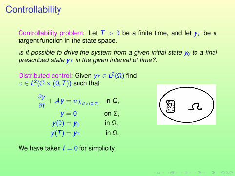
Controllability problem: Let T > 0 be a finite time, and let yT be atargent function in the state space.

Is it possible to drive the system from a given initial state y0 to a finalprescribed state yT in the given interval of time?.

Distributed control: Given yT ∈ L2(Ω) findυ ∈ L2(O × (0,T )) such that

∂y∂t

+A y = υ χO×(O,T )in Q,

y = 0 on Σ,

y(0) = y0 in Ω,

y(T ) = yT in Ω.

We have taken f = 0 for simplicity.

Exact and approximate controllability

Exact controllability

The system is controlable (or axactly controlable) when there exists acontrol υ for each target yT .

Exact controllability es very strict and it is not always possible. So, inpractice the condition y(T ) = yT is relaxed by the less restricted

Approximate controllability

In this case we look for a control υ that drives the system, in a finitetime T > 0, to a state y(T ; υ) within a small neighboorhood of yT .

More precisely: Let B be the unit ball in L2(Ω), we look for a control υsuch that

y(T ; υ) ∈ yT + εB, for ε small.

Reformulation as an optimal control

The following density result tell us that, for the approximate controla-bility problem, there are infinitely many possible controls.

If υ spans L2(O×(0,T )), then y(T ; υ) spans an affine dense subspacein L2(Ω).

We compute the control with minimal norm:

inf12

∫ T

0

∫Ω

υ2 dx dt , υ ∈ L2(O × (0,T )), y(T ; υ) ∈ yT + εB

This problem has a unique solution. Moreover

I T > 0, can be choosen arbitrarily small.

I O ⊂ Ω, may be choosen arbitrarily small.

Penalization

Alternative: The optimal control problem can be reformulated:

inf Jk (υ) =12

∫ T

0

∫Ω

υ2 dx dt +k2‖y(T ; υ)− yT‖2

L2(Ω) υ ∈ L2(O×(0,T )).

Result: There exists k large enough, such that the minimun uk of Jkverifies:

‖y(T ; uk )− yT‖ ≤ ε (k ∝ 1/ε)

I The solution can be reached by methods acting directly on thecontrol υ.

I We can also apply convex duality theory.

Optimality system

The minimum uk of Jk (υ) satisfies the following optimality system:

∂y∂t

+A y = ψ χO×(O,T )in Q, y(0) = 0, y = 0 sobre Σ

−∂ψ∂t

+A∗ ψ = 0 in Q, ψ(T ) = k (yT − y(T )), ψ = 0 on Σ.

uk = ψ χO×(O,T )

Operational formulation

1. Define the following operator Λ : L2(Ω) −→ L2(Ω):

Λ g = yg(T ),

where given g ∈ L2(Ω), we obtain

I ψg , form the solution of

−∂ψ∂t

+A∗ ψ = 0 en Q, ψ(T ) = g, ψ = 0 sobre Σ.

I yg , from the solution of

∂y∂t

+A y = ψg χO×(O,T )en Q, y(0) = 0, y = 0 sobre Σ

2. If we denote k (yT − y(T )) by u, then u solves

(k−1I + Λ) u = yT .

The operational equation

Lu = yT , with L =(k−1I + Λ

)is the Euler–Lagrange equation of a quadratic minimization problem,

then we can apply a gradient descent method to solve it.

Once u is obtained, the control is found by solving first

−∂ψ∂t

+A∗ ψ = 0 en Q,

ψ(T ) = u, en Ω,

ψ = 0 sobre Σ.

Therefore, the control is uk = ψ χO×(O,T ).

Comjugate gradient algorithm

1. Inicialization: Given u0, compute g0 = Lu0 − yT and d0 = −g0.

2. Descent: Assuming we know uk , gk , dk , find uk+1, gk+1,dk+1

doing the following

uk+1 = uk + αk dk , with αk =〈gk , gk 〉〈dk , Ldk 〉

gk+1 = gk + αk Ldk

Test of convergence: If ‖gk+1‖ ≤ ε‖g0‖, take u∗ = uk+1 andstop. Otherwise, go to step 3.

3. New conjugate direction

dk+1 = −gk+1 + βk dk , with βk =〈gk+1,gk+1〉〈gk , gk 〉

Do k = k + 1 and go to step 2.

Numerical examplesIn all cases we solved the state and adjoint equations by the finiteelement method with ∆x = ∆ t = 0.01.

∂y∂t− ∂2y∂x2 = υ χO×(0, T )

in Q = (0,1)× (0,T ),

y = 0 on Σ = Γ× (0,T )

y(0) =

x , x ≤ 1/2;1− x , x > 1/2.

y(T ) = yT

Example 1. (smooth target) yT = 4x(1− x)

Example 2. (nonsmooth target) yT =

8(x − 14 ), if 1/4 ≤ x ≤ 1/2,

8( 34 − x), if 1/2 ≤ x ≤ 3/4,

0, otherwise.

Example 3. (nonsymmetric target) yT = 4 x (1− x) (x − 1/8)

Example 1. Smooth target

yT = 4x(1− x)

|y(T )−yT ||yT | = 0.03 Evolution of the control υ

I Subdomain: O = (0.4, 0.6).

I Final time: T = 2.

I Tolerance: ε = 10−10

Example 2. Nonsmooth target

|y(T )−yT ||yT | = 0.21 Evolution of the control υ

I Subdomain: O = (0.4, 0.6).

I Final time: T = 2.

I Tolerance: ε = 10−10

Example 3. Nonsymmetric target

|y(T )−yT ||yT | = 0.0012

I Subdomain: O = (0, 1).

I Final time: T = 1.

I Tolerance: ε = 10−10

Pointwise control

Problem: Given yT , find υ and y such that

∂y∂t− µ

∂2y∂x2 = υ(t)δ(x − b) in Q = (0,1)× (0,T ),

y = 0 on Σ = Γ× (0,T ),

y(0) = 0y(T ) = yT

I The state equation has a unique solution for each υ ∈ L2(0,T ).

I For d ≤ 3, y ∈ L2(Q), and ∂y∂t ∈ L2(0,T ; H−2(Ω)).

I t −→ y(t ; υ) is continuous from [0,T ] into H−1(Ω).

I When υ spans L2(0,T ) then y(T ) = y(T ; υ) spans a subspaceof H−1(Ω)

Orthogonal of the closure of y(T ; υ)υ∈L2(0,T )

〈y(T ; υ), f 〉 =

∫ T

0ψ(b, t) υ(t) dt , f ∈ H1

0 (ω).

I 〈·, ·〉 is the duality pairing between H−1(Ω) and H10 (Ω).

I ψ is the solution of the adjoint equation

−∂ψ∂t

+A∗ψ = 0 in Ω, ψ(T ) = f , ψ = 0 on Σ.

I ψ ∈ L2(0,T ; H2(Ω) ∩ H10 (Ω)).

Therefore, f is ortogonal to y(T ; υυ∈L2(0,T ) ⇐⇒ ψ(b, t) = 0

and

y(T ; υ) spans a dense subset of H−1(Ω) when υ spans L2(0,T )⇐⇒b is such that ψ(b, t) = 0 implies ψ = 0.

Strategic points

Let ωj∞j=1 be the eigenfunctions of A = A∗, and λj∞j=1 thecorresponding eigenvalues.

We say that b is an strategic point in Ω if ωj (b) 6= 0 for all j = 1,2, . . ..

Then ψ(b, t) = 0 implies ψ = 0, since

ψ(x ,T ) = f (x) =∑

j

fj ωj (x), for f ∈ H10 (Ω),

ψ(b, t) =∑

j

fj ωj (b) e−λj (T−t) = 0, only if fj = 0 ∀ j .

Optimal controlSuppose b ∈ Ω is an stategic point. We look for the solution of

infυ∈V

J(υ) =12

∫ T

0υ2 dt

with V = υ ∈ L2(0,T ) : y(T ; υ) ∈ yT + β B−1, and yT ∈ H−1(Ω)and B−1 the unit ball in H−1(Ω).

This problem can be solved using duality arguments. However, fromthe practical point of view, it is easier to solve directly the followingpenalized problem

minυ∈L2(0,T )

Jk (υ) =12

∫ T

0υ2 dt +

k2‖y(T ; υ)− yT‖2

−1, k > 0,

where ‖g‖−1 = ‖ϕg‖H10 (Ω) and ϕg solution of

−4ϕg = 0 in Ω, ϕg = 0 in Γ.

Optimality conditionsThe previous problem has a unique solution u ∈ L2(0,T ), characteri-zad by the existence of p ∈ L2(0,T ; H2(Ω)∩H1

0 (Ω))∩C0([0,T ]; H10 (Ω)),

such that u, y ,p satisfies the following optimality system

∂y∂t

+A y = u δ(x − b) in Q, y = 0 on Σ, y(0) = 0,

−∂p∂t

+A∗ y = 0 in Q, p = 0 on Σ, p(T ) = k(−4)−1(yT − y(T ; u)),

u(t) = p(b, t).

This problem, or equivalently the minimization problem, can be solvedby a gradient descent method, since we can compute its derivative(first variation)∫ T

0J ′k (u) υ dt =

∫ T

0(u(t)− p(b, t)) υ(t) dt , ∀ υ ∈ L2(0.T ).

We apply a conjugate gradient algorithm very similar to the one intro-duced before.

Example 1.

Target function

yT =

8(x − 1

4 ), if 14 ≤ x ≤ 1

2 ,

8( 34 − x), if 1

2 ≤ x ≤ 34 ,

0, otherwise.

Parameters

T = 3, ∆x = ∆t = 10−2.

b k N. Iter ||uk (x ,T )||2L||yT−ym(T )||L2(Ω)

||yT ||L2(Ω)√2

3 103 3 34.1939 0.6249104 4 61.7933 0.3942105 6 79.3059 0.2789106 10 114.3000 0.2184108 26 700.2412 0.14151010 103 3.0216×103 0.1242

12 103 3 34.2446 0.6193

104 4 61.8262 0.3766105 6 82.3173 0.2251106 8 122.8655 0.1289108 15 194.5858 0.05851010 30 874.9293 0.0340

π6 103 3 34.2239 0.6246

104 4 61.8236 0.3934105 6 80.0432 0.2762106 10 115.5124 0.2178108 25 670.0066 0.14221010 144 2.7191×103 0.1235

Example2.

Unsymmetric target

yT =274

x2 (1− x) ,

Same parameters

b k N. Iter ||uk (x ,T )||2L||yT−ym(T )||L2(Ω)

||yT ||L2(Ω)√2

3 105 6 73.8552 0.3859106 11 154.3000 0.3444108 37 1.4870×103 0.14361010 105 2.3732×103 0.02281012 91 2.4727×103 0.01641015 89 2.4743×103 0.0164

12 105 6 65.2239 0.3731

106 7 78.0479 0.3572108 14 103.5828 0.35371010 15 128.9864 0.35361012 15 130.0881 0.35361015 15 130.0995 0.3536

π6 105 6 62.9638 0.3455

106 10 98.5060 0.3231108 26 1.3323×103 0.15251010 60 2.3923×103 0.02671012 61 2.5580×103 0.01921015 61 2.5606×103 0.0192

Chattering Control

The eigenfunctions associated to operator A = −µ ∂2

∂x2 , with homogeneosDirichlet boundary conditions are:

ωj (x) =sin(jπx)

|| sin(jπx)||L2(Ω). (1)

In order to be able to control de system, the control point b must be an strate-gic point :

sin(jπb) 6= 0 ∀j ∈ N,

that is, b ∈ I.

Computers don’t “know” irrational numbers, and it is necessary to move thecontrol point in order to rebuild the control, avoiding tha anulation of all eigen-functions. For instance, we can move the control point b in an oscillatory way:

c(t) = b + ε sin (2πf t) , b ∈ Q,

with ε > 0, f > 0.

No chattering

Chattering

Target function

yT =274

x2(1− x),

ParametersT = 3, ∆x = ∆t = 10−2,

b = 1/2

ε k N. Iter||yT−ym(T )||L2(Ω)

||yT ||L2(Ω)

0 105 6 0.3731106 7 0.3572108 14 0.35371010 15 0.3536

0.001 105 6 0.3731106 10 0.3551108 37 0.25811010 111 0.0859

0.08 105 10 0.2843106 18 0.1741108 95 0.04661010 530 0.0162

0.1 105 9 0.2669106 20 0.1510108 170 0.0406

No chattering

Chattering

Target function

yT =

8(x − 1

2 ), if 14 ≤ x ≤ 3

4 ,

8(1− x), if 34 ≤ x ≤ 1,

0, otherwise.

Parameters

T = 3, ∆x = ∆t = 10−2, b = 1/2

ε k N. Iter||yT−ym(T )||L2(Ω)

||yT ||L2(Ω)

0 105 6 0.7617106 7 0.7218108 22 0.70941010 29 0.7079

0.001 105 6 0.7627106 10 0.7180108 46 0.49921010 218 0.1397

0.08 105 10 0.5898106 23 0.3135108 136 0.0790

0.1 105 9 0.5488106 20 0.2636108 143 0.0675