P.K. Gupta, Sunitha Ravi Volatility Spillovers in Indian ... · Commodity markets in India have a...

P.K. Gupta, Sunitha Ravi

Centre for Management Studies, Jamia Millia Islamia University, New Delhi & Institute of Information Technology and Management, Affiliated to GGSIP University, New Delhi(India)

Volatility Spillovers in Indian Commodity Futures Markets and WPI Inflation

Abstract

Spurt in the growth in the volumes of commodity markets in India is cause of concern for the producers, regulators, market participants and society at large. Galloping prices of commodities globally and in India in the last few years has raised questions on the demand supply balances and also on the performance of commodity spot and derivative markets. A logical feeling of arbitrage and inefficiency cannot be ruled out. Evidence of volatility in the spot markets and consequent impact on inflation measured by Wholesale Price Index (WPI) raises concerns on the activities of speculators, hoarders and black market profits. Inflation is national and global concern to the governments and political fate of the leaders especially in India. We explore whether the efficiency exists between commodity futures and spot markets using the data derives for three commodity exchanges MCX, NMCE and NCDEX. We, further examine the association between the spot price of commodities and WPI. We find evidences of efficiency in most of the sample commodities, though it may depart in some time periods and establish that huge volatility of spot prices and other

market imperfections and irregularities are responsible for lifting WPI.

Keywords: Inflation, Futures , Derivatives, Commodity exchanges, Volatility, Macro Economic Impacts

1. Introduction

Gradual evolution of commodity markets in India has been of great significance for both the country’s general economic distribution and its linkages with financial sector. Being a unique hedging instrument, it provides for efficient portfolio management arising from diversification benefits, which result in improved returns to domestic as well as international investors.

From 1952- 2002 commodity derivatives market was virtually nonexistent, except some negligible activities on OTC basis (Ahuja, 2006). During the last few years commodity derivative markets in India developed at an astonishing pace especially after the introduction of nationwide electronic trading and market access, which can be observed in terms of the number of commodities traded volume, number of market participants and the growth in the number of commodity exchanges. Agricultural commodities, bullion, energy, and base metal products account for a large share of the commodities traded in the commodities futures market (Exhibit 1&2).

Commodity markets in India have a huge potential since Indian economy is conventionally an agricultural based economy. Commodity market can influence the whole economy of a country through important macroeconomic variable like inflation. India is one of the few countries where the wholesale price index is considered as the headline of inflation. In spite of various advantages of

IISES 2013 International Journal of Economic Sciences Vol. II (No.3)

36

commodity futures contract, the reopening of commodity futures trading in India in 2003 has become an important issue due to increasing rate of inflation in commodities in India and also for the volatile cash market. Persistent inflationary pressures in global commodity prices have often been high lightened over its nature with speculation, and, are considered as the prime cause of increase in prices. Though the volume of commodity trading in India increased exponentially since its reopening in 2003, the functioning of the futures market came under scrutiny during 2008-2009 due to price rise. The study examines the efficiency of spot and futures markets and the the impact of commodity spot prices on WPI inflation.

2. Literature Review

Various researches have been conducted to examine the market efficiency, association between spot and futures market, price discovery and volatility spillovers, and macro-economic impacts pertaining to commodity markets and also for stock markets. In India relatively few studies on Commodity Market Efficiency and macro-economic impact on commodity trading have been conducted. Market efficiency is a necessary condition for forecasting future prices of commodities; many researchers examine different aspects of market efficiency using various time series techniques. In an emerging-market context, the growth of commodity future market would depend on the efficiency of the future market. The success of spot and futures markets performing the stabilizing function critically depends on whether they are efficient (Fama 1970). Holbrook (1949) argues that futures price of a commodity depends on the future events that could affect the demand and supply of traded commodities. So, based on the market information, a highly organized commodity exchange is needed for better functioning of the commodity futures market. If the information were biased, there would be the possibility random or mean reversion of commodity futures price. Dusak (1973) have examined whether speculators in a futures market earn a risk premium with the context of Capital Asset Pricing Model. The systematic risk was estimated for a sample of wheat, corn and soybean futures contracts over the period 1952-1967 and found to be close to zero in all the three commodities. Average realized holding period returns on the contract over the same period were close to zero. Jagannathan (1985) have examined whether two-month returns to futures speculation for three commodities (corn, wheat, and soybeans) for the 1960-1978 periods are consistent with the consumption-beta model of risk premium, however the evidence suggested that this model did not provide an adequate description of returns to futures speculation.

Allen and Som (1987) in their paper seek to establish whether the efficient markets theory can be applied to the London Rubber Market by analyzing the price changes observed in that market for daily cash and future price series during the periods January 1975 to June 1983, and January 1980 to May 1983. The analysis features an examination of the return distributions and parametric, non-parametric and econometric tests based on auto correlation coefficients run test and filter tests. The results support the hypothesis of weak form efficiency. Canarella and Pollard (1987) tested the efficiency of Commodity Futures in a Multi Contract framework. The study examined the Efficient Market Hypothesis in both a single contract and multi contract framework for five agricultural commodities corn, wheat, soybean oil, soybean meal and soybeans. The empirical evidence points to the conclusion that the relationships between spot and future prices over different contracts that are traded simultaneously do not confirm to the predictions of the EMH. Barua (1987), Chan et al (1997) observed that the major Asian markets were weak form inefficient. Similar results were found by Dickinson and Muragu (1994) for Nairobi Stock Market. Elam and


37

Dixon (1988) have shown the invalidity of conventional F tests for market efficiency estimation for non-stationary time series modeling. Yalawar (1988) also examined a number of stocks using correlation test and run test and supported the hypothesis of efficient market. Brorsen, Oellermann and Farris (1989) investigated the direct impact of futures trading on the live cattle spot market. They conclude that the introduction of futures trading in live cattle improved spot market efficiency, but also increased short-run spot price risk. Oellermann, Brorsen and Farris (1989) have investigated dominance for feeder cattle using daily price data over an eight-year period divided into two sub periods of four years each to account for structural change. The authors found that feeder cattle futures price led spot price in incorporating new pricing information indicating that the futures market serves as the centre of price discovery for feeder cattle. Using the Garbade Silber framework, the authors found that futures market exhibited strong dominance over spot market in the first sub period and weak dominance in the second sub period. Studies like Weaver and Banerjee, (1990), Darrat and Rahman (1995) find that futures trading reduce and also do not increase cash price volatility. Hamao et al. (1990) shows the volatility spillover for the US and the UK stock markets to the Japanese stock market. Koontz et al. (1990) employs granger causality to examine dominance in live cattle market using weekly data dividing the sample period into three sub periods of four years each to examine the dynamic nature of dominance. Their results show changing dominance pattern due to structural change in the industry and that the price discovery process is dynamic in nature and dependent on the structure of futures and spot market indicating that the spot market was becoming less reliant on futures market for price discovery. Bessembinder and Seguin (1992) finds that stock market volatility is inversely related to both the open interest and trading volume of S&P 500 futures after controlling for spot market volume. They establish that spot volatility is positively related to unexpected volume and negatively related to expected open interest for eight currencies, interest rate and commodity futures contracts. For the currency and agricultural contracts, spot volatility decreases when unexpected open interest increases. Their results indicate that futures trading increase the depth and liquidity of the underlying asset market, mitigating the impact of volume shocks on volatility.

Kaminsky and Kumar (1990) have investigated the efficiency of commodity futures markets. The study analyzed the operations of the futures markets for a number of commodities over 1976-88, and tests several hypothesis about the efficiency of the markets and establsh that for certain commodities expected excess returns to futures speculations are non-zero, particularly for forecast horizons for more than three months. Fama and French (1987) tested for evidence of whether or not commodity futures prices provided forecast information superior to the information contained in spot prices. They found that futures markets for the seasonal commodities contain superior forecast power relative to spot prices. However, this was not the case for non-seasonal commodities. Becker and Finnerty (2000) establish that the inclusion of long commodity futures contracts in portfolios improved the risk and return performance of stock and bond portfolio. They observed that the commodities are certainly as an inflation hedge. Jensen, Mercer and Johnson (2000) have examined the diversification benefit of adding commodity futures to a traditional portfolio that consists of foreign equities, corporate bonds and treasury bills and find that commodity future sustainability enhances portfolio performance for investors, and, that managed futures provide the greatest benefit. Pandey (2005) have proposed a multivariate vector error correction generalized autoregressive conditional Heteroskedasticity model to investigate the effect of oil seeds and wheat grain prices in neighboring countries of Asia on its Indian equivalents. Gorton and Rouwenhorst (2006) explore that commodity futures returns are negatively correlated with equity and bond


38

returns. They argued that their negative correlation between commodity futures and the other assets classes is due, in significant part, to a different behavior over the business cycle. They further establish that commodity futures are positively correlated with inflation and changes in expected inflation. Aggarwal et. al (2007) explores the inter linkages between macroeconomics and agro commodity prices using Cointegration model and OLS model to examine the relationship between GDP, wholesale price index and agricultural yield and prices, five major crops were selected namely, rice, wheat, cotton, sugar and oilseeds. The results conclude that for sugar and cotton the degree of correlation with WPI is low. Macroeconomic influences are minimal or remain obvious to the changes in agricultural prices and yield.

Sen (2008) have studied the role of futures trading on the wholesale and retail prices of agricultural commodities in the wake of consistent rise of rate of inflation during the first quarter of 2007. The analysis of 21 agricultural commodities shown that at the annual trend growth rate in prices (using monthly and weekly data) was higher in the post futures period in 14 commodities and lower in 7 commodities. Sahoo and Kumar (2008) have examined the impact of proposed commodity transaction tax on futures trading in India using relationship between trading activity, volatility and transaction cost, through a three equation structure model for five top selected commodities, namely, Gold, Copper, Petroleum Crude, Soya oil and Chana. Results suggest that there exists a negative relationship between transaction cost and volatility. Granger causality test reveals the efficiency of futures markets but does not provide any conclusive evidence about the nexus between price rise and futures trading. Bose (2009) analyzes the role of futures market in aggravating commodity price inflation and the future of commodity futures in India. Investigations carried out by the US Commodity Futures Trading Commission and the Indian Expert Committee on futures trading found that no conclusive proof could be established regarding the role of futures market in India or in the US.

Nayak (2010) analyzes different sources of agricultural commodity price fluctuations and their macroeconomic implication for developing countries in general and India. The study tries to examine two sector macroeconomic models for different commodities produced in the agricultural and allied sectors and their future prices. The paper also explores the possibilities of different commodities produced in the economy and their distribution in a dual economic structure, which is open to international trade. The result of the study reveals that for many commodities future price fails to provide an efficient price structure and the risk emerging from the fluctuation in the prices. The study also reveals that in some agricultural commodities traded in exchange, future market price is not stable and not efficient from macroeconomic point of view.

Srinivasan (2012) examined the price discovery process and volatility spillovers in Indian spot-futures commodity markets through Johansen Cointegration, Vector Error Correction Model (VECM) and the bivariate EGARCH model. The study uses four futures and spot indices of the Multi Commodity Exchange of India (MCX), representing relevant sectors like agriculture (MCXAGRI), energy (MCXENERGY), metal (MCXMETAL), and the composite index of metals, energy and agro commodities (MCXCOMDEX). Johansen Cointegration test confirms the presence of long-term equilibrium relationships between the futures price and its underlying spot price of the commodity markets. The VECM shows that commodity spot markets of MCXCOMDEX, MCXAGRI, MCXENERGY and MCXMETAL play a dominant role and serve as effective price discovery vehicle, implying that there is a flow of information from spot to futures commodity


39

markets. Besides, the bivariate EGARCH model indicates that although bidirectional volatility spillover persists, the volatility spillovers from spot to the futures market are dominant in case of all MCX commodity markets.

There is a vast amount of literature on market efficiency considering the stock markets in developed as well as developing countries including India. Few quantitative studies have been conducted to test the efficiency of Commodity Markets worldwide and particularly in the Indian context especially during the period of severe inflationary pressure. We are therefore motivated to study the efficiency of commodity Futures Market in India and its inflationary impacts.

3. Data and Methodology

In order to test the macro-economic impacts, the data for monthly Spot prices of the commodity Chana, Gaurseed, Wheat, Potato and Cottonseed oil cake traded has been taken from National Commodity Derivative Exchange (NCDEX). In India, NCDEX is considered as prime national level commodity exchange for agricultural commodities and hence selected for empirically examining the causality between spot prices and WPI inflation for a period starting from 2005 to April 12, 2012. Monthly data for Wholesale Price Index (WPI) inflation (base year 2004-2005) has been taken from Office of the Economic advisor, Government of India.

To test the volatility spillovers, we use the samples for five commodities actively traded in three national level multi commodity Exchanges in India (NCDEX, MCX and NMCE) for a period of 2005 to 2012. The selected commodities are Chana, Gaurseed, Refsoyoil, Gold and Silver. In Spot as well as future prices, the last price or the closing price is considered for the study. Spot price of the Commodities selected for macroeconomic study is converted to a representative monthly figure by taking the arithmetic average for all quoted closing prices for a given month.

Granger Causality Test

A statistical approach proposed by Clive W Granger (1969) to infer cause and effect relationship between two (or more time series) is known as Granger causality. It use F test to study find the right direction of variable. Granger Causality is based on the simple logic that effect cannot precede cause. It is important to note that the statement “x Granger causes y” does not imply that y is the effect or the result of x. Granger causality measures precedence and information content but does not by itself indicate causality in the more common use of the term. Granger causality is a necessary condition for causality, but not a sufficient condition. The test itself is just an F test of the joint significance of the other variable(s) in a regression that includes lags of the dependent variable.

In its original form it is based on following bivariate regression model (there are some other procedures used for causality testing such as Sim’s Causality test, Hasiao Causality Test etc.)

t

I

jjtj

I

iititt

I

jjti

I

iitit yxxxyy εθγωεβαα ∑∑∑∑

=−

=−

=−

=− +++=+++=

11110 ;


40

If all the coefficients of x in first regression equation of y , i.e. i b for i =1......l are significant that the null hypothesis that x does not cause y . However, the significance of the coefficient cannot be evaluated based on usual t-statistic. Procedure for testing the nested models is - estimate the model without including lagged values of variable x. Suppose the R

2 from this estimate is R21 . Now estimate the model including lagged values of variable x. Suppose the R

2 from this estimate is R22 .

F-ratio for improvement in the model is - )/()1(

/)(22

21

22

knR

kRRF

−−−= ; Where k* are the number of lag

orders l of variable x, k is the total number of the parameters estimated and n is the number of observations. The null hypothesis of non-causality is rejected if F statistic is greater than its critical value at k* and (n-k) degree of freedom. Similarly from the second equation above, we can test the null hypothesis that ‘y does not cause x’. If only one of the two variables causes the second variable but the second variable does not cause the first variable, it is called one-way causality else both ways it is called the feedback causality.

Block Exogenity Wald test

In block erogeneity the causality can be evaluated by examining the joint significance of lagged coefficients of one variable in the equation of another variable. In context of the bivariate case presented above the causality can be examined by testing the following hypothesis using Wald test. Tests of this form were described by Granger (1969) and a slight variant due to Sims (1972). Causality tests seek to answer simple questions of the type, ‘Do changes in y1 cause changes in y2?’ The argument follows that if y1 causes y2, lags of y1 should be significant in the equation for y2. If this is the case and not vice versa, it would be said that y1 ‘Granger causes’ y2 or that there exists unidirectional causality from y1 to y2. On the other hand, if y2 causes y1, lags of y2 should be significant in the equation for y1. If both sets of lags were significant, it would be said that there was ‘bi-directional causality’ or ‘bi-directional feedback’. If y1 is found to Granger-cause y2, but not vice versa, it would be said that variable y1 is strongly exogenous (in the equation for y2). If neither set of lags were statistically significant in the equation for the other variable, it would be said that y1 and y2 are independent. The block exogenity test also measures the speed of adjustment of prices towards the long run equilibrium relationship. The block exogenity test is applied in order to analyze the short run causal relationship exists between the spot prices and future price of the commodities.

Impulse Response Function

Impulse-response function simulates the effects of a shock to one variable in the system on the conditional forecast of another variable. It explains the impact of an exogenous shock in one variable on the other variables of the system. The researchers use the impulse-response function to analyze the impact of change in one variable (say future price) on other variables (spot price). Impulse responses trace out the responsiveness of the dependent variables to shocks to each of the variables. So, for each variable from each equation separately, a unit shock is applied to the error, and the effects upon the system over time are noted. Thus, if there are g variables in a system, a total of g2 impulse responses could be generated. An IRF allows one to trace the time path of the impact of a shock in one variable on all the variables contained in the system. However, the


41

standard impulse response analysis assumes that the shock occurs in one variable at a time. Such an assumption may be valid only if the shocks in different variables are not correlated.

Volatility Spillovers and E-GARCH Model

Measurement of volatility is an important issue in financial commodity market in India. Volatility refers to the degree of fluctuations or the variability of a variable around its mean; where mean may be a constant or varying with time or other variables. Statistically, volatility is equivalent to dispersions and if it is assumed that it is time invariant (as it is generally assumed in classical regression models), it can be measured as the standard deviation or the variance. However, when this assumption is relaxed and realizes that variability of asset returns change with time (sometimes market becomes highly volatile and sometimes it remains in the state of tranquility), then the measurement of volatility becomes little bit involving. In an arbitrage free economy, price volatility is directly related to the flow of information and will rise due to the conditionality of increasing flow of information, thereby, generating the volatility in the spot market. The volatility spillovers reveal that future trading could intensify volatility in the underlying spot market, perhaps due to the larger trading program and the speculative nature of the future trading. The volatility spillovers hypothesis involves testing for the lead-lag relations between volatilities in the futures and spot markets.

Generalized Autoregressive Conditional Heteroskedasticity (GARCH) model

The GARCH model was developed independently by Bollerslev (1986) and Taylor (1986). The GARCH model allows the conditional variance to be dependent upon previous own lags, so that the conditional variance equation in the simplest case is now

= (a)

This is a GARCH (1, 1) model. is known as the conditional variance since it is a one-period ahead estimate for the variance calculated based on any past information thought relevant. Using the GARCH model it is possible to interpret the current fitted variance, ht, as a weighted function of a long-term average value (dependent on α0), information about volatility during the previous period and the fitted variance from the model during the previous period

Note that the GARCH model can be expressed in a form that shows that it is effectively an ARMA model for the conditional variance. To see this, consider that the squared return at time t relative to the conditional variance is given by

=

or

=


42

Substitute the value of in equation (a) for conditional variance

=

Rearranging

So that

This final expression is an ARMA (1,1) process for the squared errors. Where measures the persistence of volatility? In practice, this usually observed very close to 1, which signifies that the volatility of asset returns is highly persistent. The effect of any shock in volatility dies out at a rate of . If ≥ 1 the effect of shock will never die out. The volatility will be defined only if <1. Therefore, this condition is imposed while estimating the GARCH model.

The EGARCH model and the Volatility Spillover

D.B. Nelson (1991) proposed the exponential GARCH (EGARCH) model. Conditional variance equation is given by

The model has several advantages over the pure GARCH specification. First, since the log ( ) is modeled, and then even if the parameters are negative, will be positive. There is thus no need to artificially impose non-negativity constraints on the model parameters. Second, asymmetries are allowed for under the EGARCH formulation, since if the relationship between volatility and returns is negative, γ, will be negative. However, owing to its computational ease and intuitive interpretation, almost all applications of EGARCH employ conditionally normal errors as discussed above rather than using GED.

Nelson’s (1991) exponential GARCH (EGARCH) model is used in order to capture the asymmetric impacts of shocks or innovations on volatilities and to avoid imposing non-negativity restrictions on the values of GARCH parameters (Bollerslev) to be estimated. The need for this approach, as opposed to the now common GARCH specification, is explained by Bae and Karolyi (1994) and Koutmos and Booth (1995), who collectively report that the volatility transmission between U.S., U.K. and Japanese stock markets is asymmetric. Moreover, the EGARCH model allows negative shocks to behave differently than the positive shocks. In this study, the estimation


43

process is not concentrated about the return series but about the direct spillover between futures and spot markets for MCX, NCDEX and NMCE in Indian commodity market.

4. Results and Discussions

1.1 Pair wise Granger Causality Test Results

We show the results of granger casualty test of spot and future prices on WPI inflation. The price series of the selected commodities on NCDEX were examined for stationarity for all commodities. The series is non-stationary; therefore its returns are used to analyze the causal effect on commodity trading and inflationary impacts. Pair wise granger causality test has been used to analyze the causal relationship between the commodity prices and inflation. The result of the Granger Causality for respective commodities is shown in Table 1-5.

Chana shows high value of F-statistics indicating that the changes in prices in Chana have a significant impact on the WPI inflation. The causality test is unidirectional. In case of Gaurseed, also the changes in prices have a significant impact on the Gaurseed WPI inflation. In first lag causality is birectional whereas in second and third lags the causality is unidirectional.

Wheat WPI does not Granger cause Wheat Spot is significantly high and the p value of f statistics is less than 5% level of significance. This indicates that the changes in WPI inflation in Wheat have a significant impact on the Wheat Price.

In case of Potato there is no causality in both directions. It is derived from the results that the changes in WPI inflation in Potato do not have a significant impact on the Potato Price and the reverse. This result is very important because a large chunk of low-income group population inherently consumes potato and onions whose price also affect the political fate domestically.

The results in case of commodity Cottonseed Oil cake in NCDEX also show that in both directions there is no causality. It is therefore concluded from the results that the changes in WPI inflation in cottonseed oil cake do not have a significant impact on the cottonseed oil cake Price and the vice-versa. We therefore see that in some selected commodities there exists significant causal relationship between the spot prices to Wholesale Price Index Inflation caused for the Commodities in India.

Block Exogenity Wald Test Results

Block Exogenity Wald Test has been carried out to examine the causality between commodity prices and the wholesale price index of the commodity. The results are shown in Table 6-10.

In case of Chana, 2χ observed for the causal relationship between spot prices to WPI

inflation is 35.46525(p=0.00) indicating that the spot prices are exogenous in nature but the past prices of the spot influences the WPI inflation of the Chana in the future. Gaurseed results show that


44

the causality comes from spot prices to WPI inflation (2χ =23.29, p=0.5119) implying that the spot

prices are exogenous in nature but the past prices of the spot influences the WPI inflation of the Gaurseed in the future.

Potato results reveal that in spot prices to WPI inflation and WPI inflation to Spot, there is

no causal impact (2χ =4.11; p=0.1281). Both the directions values are not significant. It can be

concluded that there is no causal impact in both the cases in case of Potato. In case of Wheat the

result indicate that the causality comes from WPI inflation to spot prices (2χ =2.47; p=0.4798). It

can be concluded that the WPI inflation are exogenous in nature but the past prices of the Inflation influences the spot prices of the wheat in the future. However for cotton in both the directions values are not significant implying that there is no causal impact in both the cases in cotton.

Overall, it can be concluded that the past prices of spot influence the WPI inflation in commodities Chana, Gaurseed and Wheat. There is no causal impact between WPI inflation and Spot prices of commodities Potato and Cottonseed oil cake.

Impulse Response Function Results

Results from Granger Causality and Block Exogenity test verified through Generalized Impulse response Functions (GIRF). The GIRF trace the effect of one a one-time shock to one of the innovations on inflation and spot prices of commodities. The GIRF illustrates the impact of a unit shock to the error of each equation of the VAR. The results of the Generalized Impulse response Function (GIRF) between commodity spot prices and WPI inflation of all commodities are shown in Figure 1-5. The result of Impulse response function confirms the results of Wald test in all the selected commodities. Plotting the GIRF is a way to explore the response of a variable to a shock immediately with various lags. Unlike the orthogonalised Variance Decomposition and IRF obtained using the Cholesky factorization, the GIRF’s are unique and invariant to the ordering of the variables in the Vector Auto Regressive Model.

This finally indicates that the results of GIRF for all the selected Commodities shows that there exists significant causal relationship between the spot prices to Whole sale Price Index Inflation caused for the Commodities in India.

Volatility Spillover Results

Pairwise Granger Causality Test, Block exogenity test and Impulse Response Function examine the information transmission between markets by investigating first movement (mean return). However, examining the second movement or volatility spillover across markets better captures the information transmission. The EGARCH model has been used to analyze the volatility spillover impact between spot and future market for respective commodities (Table 11-15). Volatility Spillover effect implies that if volatility comes in one markets on a particular day it will influence the volatility of the other market on the next day.

Chana - In case of Chana, commodity exchange MCX and NMCE a significant spillover has been observed. It is observed that the previous volatility of future market has a large Impact on the volatility of spot market on next day as compared to previous volatility in spot prices on the next


45

day volatility in future prices. This result supported the proposition of price discovery in future market. However in case of NCDEX the previous volatility in Spot prices has a large impact on the volatility of Future prices on next day as compared to previous volatility in future price on the next day volatility in spot price.

Gaurseed - The coefficients describe the volatility spillover from the spot to futures and futures to spot. Results indicate that for commodity exchanges NCDEX and NMCE coefficients are all significant, because coefficient spot is larger than the coefficient in futures market. However in case of MCX the volatility in spot prices at one lag earlier has a higher impact on the volatility of future prices on any particular day as compared to previous volatility in future prices on the next day volatility in spot price. Since NCDEX trading volume of agri-commodities is highest, it can be concluded that the spot market volatility in the commodity market in case of Gaurseed is significantly influenced by the volatility in the future prices at previous lag.

Ref Soyoil - The direction of volatility spillover in NCDEX and NMCE is from future to spot market since the coefficient of spot is higher than the coefficient of future market in case of Ref Soyoil. If future market increases the flow of information, volatility in the underlying spot market will rise. This implies that the volatility of the asset price will rise as the rate of information flow increases. The results confirm the theory of price discovery.

Gold - It is observed that the previous volatility of future market has a large impact on the volatility of spot price on next day as compared to previous volatility in spot prices on the next day volatility in futures prices in exchanges MCX and NCDEX. The findings of the study confirm that future market plays a crucial role in the Price Discovery.

Silver - The result indicates that the coefficient is significant in case of futures to spot in MCX and NCDEX exchanges. This implies bad news effect is more than good news effect for spot to futures. As both spot and futures market spill each other, shocks in one market would induce changes in volatility of another market. The results of the study indicate that the future market of the commodities is more efficient as compared to spot market.

So and therefore, market efficiency and price discovery process can be established given that cointegration is a necessary condition for market efficiency. The results support the research findings of Bose (2008) examination of metal, energy and agriculture products, Singh (2010) examination of Gaur Gum and Gaurseed and Ali and Gupta (2011) research on agricultural products but contrary to the examination of market efficiency by Singh Jatinder (2004) who says it varies across commodities. It is seen that overall the market is efficient, though for some periods or specific commodities, inefficiency may be seen that attract the researchers.

Hence, it can be derived that the future market plays an important role in the price discovery mechanism in most of the selected commodities. However, the volatility of the spot market causes huge positions to build up in futures market which further enhance the volatility in spot market in a spiral way, thus leading to high inflations as is also evident from the granger causality results.

We also argue that various legal regulatory and operational issues in commodity derivative markets show a significant inefficiency from an operational perspective. Restrictions on the


46

movement of certain goods from one state to another, differential tax treatment of speculative gains and losses discourage investors and funds from participating in official futures exchanges that affect the liquidity of the markets. We find an absence of the proper regulatory authority for accreditation of warehouses and setting standards. There is no uniformity regarding the contract size of various commodities. The delivery and settlement procedure differs for each commodity in terms of demand and supply related factors, place of delivery, quality implications, grade of the commodity, margin system, geographical factors, etc.

Stamp duties and Commodity Transaction Tax distort market. Financial institutions, banks and cooperatives are not permitted to engage in commodity futures trade. Most of the commodity exchanges act as product bourses. The regional exchanges are not integrated with the national exchanges. Hoarding of commodities is a major national issue that points out the need to revamp or effective implements the provisions of Essential Commodities Act, 1955. Since, most of the trades in commodity futures are cash settled, the impact of hoarding or supply related information could be disastrous. Efficiency in commodity futures market is also important from the perspective of national image particularly in terms of real GDP growth rate that discounts the WPI and is the basis for Foreign Direct Investments.

5. Remarks

Sharp volatility in the global commodity prices since 2008 has increased the focus on studying the impact of inflation and commodity prices. Increase in food and essential commodity prices in India sparked a debate on the role of a commodity market in influencing price trends. Inflation and financial development should be considered as the policy variables to forecast economic growth in the Indian economy. Our study shows sign of market efficiency but make spot prices of commodities responsible for rise in Wholesale Price Index inflation. We find a further research gap to analyze the legal; and regulatory framework and the bottlenecks of logistics that can throw further light to the problem of commodity drive inflation in a country like India, which is currently experiencing slowdown post global financial crises and where it is extremely important to build confidence among the people.

References

Agarwal S. Laddha P. Prashant K. and Anantha M. (2007). Opportunities and Challenges Macroeconomics and Agro Commodity Prices Using Co-Integration Model. International Conference on Agribusiness and Food Industry in Developing Countries. (IFIM, Bangalore).

Ali, Jabir and Kirti Bardhan Gupta (2011). Efficiency in Agricultural Commodity Futures Markets in India: Evidence from Causality and Cointegration tests. Agricultural Finance Review. 71 (2), 162-178.

Allen and Som (1987).On the Efficiency of the UK Rubber Market. Empec. 12,79-95.

Ahuja N. L. (2006), Commodity Derivatives Market in India: Development, Regulation and Future Prospects. International Research Journal of Finance and Economics, 2, 153-162.

Barua S K (1987). Some observations on the report of the High Powered Committee on the stock exchange reforms. Annual Issue of ICFAI. Dec.


47

Becker K and Finnerty J (2000). Indexed Commodity Futures and the Risk and Return of Institutional portfolios. Futures and Options research. Western Publishing.

Bessembinder H. and Seguin P. J. (1993). Price volatility, trading volume, and market depth: evidence from futures markets. Journal of Financial and Quantitative Analysis. 28, 21–39.

Bose Sushismita (2009). The role of Futures market in aggravating commodity price inflation and the future of Commodity Futures in India. ICRA Bulletin, Money and Finance. March 2009 http://www.icra.in/Files/MoneyFinance/ 4. %20Suchismita%20 Bose.pdf accessed on Feb 2011.

Bose, S. (2008). Commodity Futures Market in India: A Study of Trends in the Notional Multi-Commodity Indices. Money & Finance, ICRA Bulletin, 3(3).

Brooks Chris(2011). Introductory Econometrics for Finance. Second Edition. Cambridge University Press.

Brorsen B. Oellermann C M. and Farris P L.(1989). The live cattle futures market and daily cash price movements. The Journal of Futures Markets. 9(4), 273–82.

Canarella and Pollard (1987). Test of the efficiency of commodity futures in a multi-contract frame work. Empirical Economics. 12(2), 67-78.

Chan K C. Gup B E. and Pan M S (1997). International Stock Market Efficiency and Integration: A study of Eighteen Nations. Journal of Business Finance & Accounting. 24(6).

Dickinson J P. and Muragu K. (1994). Market Efficiency in Developing Countries: A Case Study of Nairobi Stock Exchange. Journal of Business Finance & Accounting. 211, 133-150.

Dusak K. (1973). Futures Trading and Investor Returns: An Investigation of Commodity Market Risk Premiums. Journal of Political Economy. University of Chicago Press. 81(6), 1387-1406.

Elam E. and Dixon B L. (1988). Examining the Validity of a Test of Futures Market Efficiency. Journal of Futures Markets. 8(3), 365-372.

Fama E. and K. French (1987). Commodity Futures Prices: Some Evidence on Forecast Power, Premiums, and the Theory of Storage. Journal of Business. 60(1), 55-73.

Gorton G and Rouwenhorst KG (2006). Facts and Fantasies about Commodity Markets. Yale ICF Working Paper No. 04-20.

Granger C W J. (1969). Investigating Casual Relations by Econometric models and Cross spectral Methods. Econometrica. 55, 251-276.

Gujarati Porter and Gunasekar (2012). Basic Econometrics. Fifth edition. Tata McGraw Hill Publications. New York.

Hamao Y. Masulis R and Ng V (1990). Correlations in Price Changes and Volatility across International Stock Markets. Review of Financial Studies. 3(2), 281-307.

Jagannathan Ravi (1985). An Investigation of Commodity Futures Prices Using the Consumption-based Inter temporal Capital Asset Pricing Model. Journal of Finance. American Finance Association. 40(1), 175-91.

Jensen G R. Johnson R R. and Mercer JM.(2000). Efficient use of Commodity Futures in Diversified Portfolios. The Journal of Future Markets. 20(5), 489-506.


48

Kaminsky Graciela and Manmohan S. Kumar (1990). Efficiency in Commodity Futures Markets. IMF Staff Papers. 37(3), 670-699.

Koontz. Stephen R. Garcia. Philip and Hudson Michael A. (1990). Dominant–satellite relationship between live cattle cash and futures markets. The Journal of Futures Markets. 10(2), 123–36.

Nayak Surath (2010). Macroeconomic of Agricultural Price Policy for India: An Empirical Study, in Velumurugan PS et al. (eds.) Indian Commodity Market (Derivatives and Risk management). Puducherry. Serials, 263.

Oellermann C M. and Farris P L. (1985). Futures or cash: which market leads live beef cattle prices? The Journal of Futures Markets. 5(4), 529–38.

Pandey A. (2005). Volatility Models and their Performance in Indian Capital Markets. Vikalpa. 30 (2). 27–46.

Sahoo P. and Kumar R. (2008). Impact of Proposed Commodity Transaction Tax on Futures Trading in India. Working paper no.216. Indian Council for International Economic relations. New Delhi. India.

Sen A. (2008). Report of the Expert Committee to Study the Impact of Futures Trading on Agricultural Commodity Prices. Government of India at http://www.fmc.gov.in accessed on 25th May 2011.

Sims C. (1972). Money, Income, and Causality. American Economic Review. 62, 540–52.

Singh, Jatinder Bir (2004). The weak form efficiency of Indian commodity futures. http://www.utiicm.com/Cmc/PDFs/2001/jatindersingh.pdf accessed on August 2010.

Srinivasan P (2012). Price Discovery and Volatility Spillovers in Indian Spot-Futures Commodity Market. IUP Journal of behavioral finance. March 2012.

Weaver R.D. and A. Banerjee (1990). Does Futures Trading Destabilize Cash Prices? Evidence for U.S. Live Beef Cattle. Journal of Futures Markets. 10, 41–60.

Working. Holbrook (1949). The Theory of the Price of Storage. American Economic Review. 39, 1254-62.

Yalawar Y. (1988). Bombay stock exchange: rates of return and efficiency. Indian Economic Journal. 35, 68–121.


49

Exhibits, Tables and Figures

Exhibit 1 - Trade in Commodity Futures Market

I tem 2009-10 2010-2011 2011-12(up to Jan’12)

Volume

(in lakh tonnes)

Value

( in crore)

Volume

(in lakh tonnes)

Value

( in crore)

Volume

(in lakh tonnes)

Value

( in crore) Agriculture 3991.21

(39.3) 1217949 (15.7)

4168 (32.6)

1456390 (12.2)

3878.45 (33.2)

1695550.8 (11.2)

Bullion 4.73 (0.05)

3164152 (40.8)

7.38 (0.1)

5493892 (46.0)

8.86 (0.1)

8758384.3 (57.7)

Metals 982 (9.7)

1801636 (23.2)

1410 (11.0)

2687673 (22.5)

1081.10 (9.3)

2311689.0 (15.2)

Energy 5163 (50.9)

1577882 (20.3)

7220.12 (56.4)

2310959 (19.3)

6714.96 (57.5)

2423261.2 (15.9)

Others 2.12(0.02) 3134(0.04) *0 29.04 *0.01 5.9

Total 10143 7764754 12805.57 11948942 11683.38 15188891.3

Source: Department of Consumer Affairs, Government of India Note: * volume of certified emission reduction (CER), electricity, heating oil and gasoline not included in the total volumes of other commodities. Figures in bracket show the percentage share to total.

Exhibit 2 - Performance Ranking of Top 7 Global Commodity Future Exchanges

Rank Commodity Exchanges 2011 (Jan-June) Volume in

million futures contracts

1 CME group (includes CBOT NYMEX)US 352.96

2 Zhengzhou Commodity Exchange (CZCE) China 217.58

3 Intercontinental Exchange (ICE)-US,UK and Canada 159.09

4 Shanghai Futures Exchange (SHFE) -China 128.54

5 MCX( Metal & Energy) India 127.77

6 Dalian Commodity Exchange (DCE)-China 123.88

7 London Metal Exchange(LME)-UK 64.52

Source: Data published for the period between January 1 and June 30, 2011 on the websites of the exchanges, use of market data and FIA volume survey.

Table 1 Results of Granger Causality Test-Chana

Null Hypothesis Lag F statistic P value Remarks Chana WPI does not Granger cause Chana Spot

1 2.22220 0.13974 H0 not rejected

2 0.21979 0.80316 H0 not rejected 3 0.22356 0.87976 H0 not rejected

Chana Spot does not Granger cause Chana WPI

1 32.1443 1.9E-07 H0 Rejected

2 17.7326 4.0E-07 H0 Rejected 3 12.0902 1.4E-06 H0 Rejected


50

Table 2 Results of Granger Causality -Gaurseed

Null Hypothesis Lag F statistic P value Remarks

Gaurseed WPI does not Granger cause Gaurseed Spot

1 7.68725 0.00675 H0 Rejected


Gaurseed Spot does not Granger cause Gaurseed WPI

1 14.5864 0.00024 H0 Rejected

2 11.6450 3.3E-05 H0 Rejected 3 7.82235 0.00011 H0 Rejected

Table 3 Results of Granger Causality Test -Wheat


Wheat WPI does not Granger cause Wheat Spot

1 2.69528 0.10635 H0 accepted

2 9.95044 0.00022 H0 Rejected 3 6.44218 0.00092 H0 Rejected

Wheat Spot does not Granger cause Wheat WPI

1 0.38518 0.53741 H0 not rejected


Table 4 Results of Granger Causality Test -Potato


Potato WPI does not Granger cause Potato Spot

1 0.39653 0.53187 H0 not rejected


Potato Spot does not Granger cause Potato WPI

1 3.73654 0.05915 H0 not rejected


Table 5 Results of Granger Causality Test - Cotton seed oil cake

Null Hypothesis Lag F statistic P value Remarks Cotton seed oil cake WPI does not Granger cause Cotton seed oil cake Spot

1 2.60188 0.11067 H0 not rejected 2 0.76919 0.46692 H0 not rejected 3 2.66417 0.05406 H0 not rejected

Cotton seed oil cake Spot does not Granger cause Cotton seed oil cake WPI

1 3.42177 0.06803 H0 not rejected 2 1.29534 0.27970 H0 not rejected 3 1.19904 0.31613 H0 not rejected

Table 6 Block Exogenity Wald Test Results-Chana

Dependent Variable Excluded df Chana Chi square P value

Chana WPI Chana Spot 2 35.46525 0.0000

Chana Spot Chana WPI 2 0.439575 0.8027


51

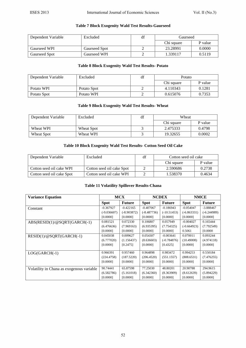
Table 7 Block Exogenity Wald Test Results-Gaurseed

Dependent Variable Excluded df Gaurseed Chi square P value

Gaurseed WPI Gaurseed Spot 2 23.28991 0.0000 Gaurseed Spot Gaurseed WPI 2 1.339117 0.5119

Table 8 Block Exogenity Wald Test Results- Potato

Dependent Variable Excluded df Potato Chi square P value

Potato WPI Potato Spot 2 4.110343 0.1281 Potato Spot Potato WPI 2 0.615076 0.7353

Table 9 Block Exogenity Wald Test Results- Wheat

Dependent Variable Excluded df Wheat Chi square P value

Wheat WPI Wheat Spot 3 2.475333 0.4798 Wheat Spot Wheat WPI 3 19.32655 0.0002

Table 10 Block Exogenity Wald Test Results- Cotton Seed Oil Cake

Dependent Variable Excluded df Cotton seed oil cake Chi square P value

Cotton seed oil cake WPI Cotton seed oil cake Spot 2 2.590686 0.2738 Cotton seed oil cake Spot Cotton seed oil cake WPI 2 1.538370 0.4634

Table 11 Volatility Spillover Results-Chana

Variance Equation MCX NCDEX NMCE Spot Future Spot Future Spot Future

Constant -0.367927 (-9.036607) [0.0000]

-0.422165 (-8.903872) [0.0000]

-0.407067 (-8.487736) [0.0000]

-0.186943 (-10.51453) [0.0000]

-0.054047 (-6.863331) [0.0000]

-3.888467 (-6.244989) [0.0000]

ABS(RESID(1)/@SQRT(GARCH(-1) 0.081521 (6.476636) [0.0000]

0.072330 (7.969163) [0.0000]

0.106807 (6.935395) [0.0000]

0.057949 (7.754325) [0.0000]

-0.004027 (-0.664923) 0.5061

0.165444 (7.792549) [0.0000

RESID(1)/@SQRT(GARCH(-1)

0.045038 (6.777020) [0.0000]

0.009627 (1.156437) [0.2475]

0.054307 (8.636603) [0.0000]

-0.003641 (-0.784876) [0.4325]

0.070011 (10.49008) [0.0000]

0.093244 (4.974118) [0.0000]

LOG(GARCH(-1) 0.966391 (224.4758) [0.0000]

0.957460 (187.5220) [0.0000]

0.964898 (206.4520) [0.0000]

0.983472 (551.1557) [0.0000]

0.994253 (808.6531) [0.0000]

0.550184 (7.476255) [0.0000]

Volatility in Chana as exogenous variable 90.74441 (6.582786) [0.0000]

65.87598 (5.161018) [0.0000]

77.25030 (6.342360) [0.0000]

48.80201 (8.363909) [0.0000]

20.90788 (8.612639) [0.0000]

294.9615 (5.894229) [0.0000]


52

Table 12 Volatility Spillover Results-Gaurseed


Constant -0.430883 (-9.676204) [0.0000]

-1.594935 (-13.24351) [0.0000]

-0.492113 (-12.66073) [0.0000]

-0.529986 (-8.616578) [0.0000]

-5.010397 (-8.989812) [0.0000]

-0.982542 (-11.22111) [0.0000]


0.194958 (14.51698) [0.0000]

0.134643 (9.156634) [0.0000]

0.058095 (4.735329) [0.0000]

-0.121540 (-5.976896) [0.0000]

0.331839 (19.71357) [0.0000]


0.051020 (5.872229) [0.0000]

-0.082843 (-6.899438) [0.0000]

0.070026 (9.640572) [0.0000]

0.034389 (4.317374) [0.0000]

0.293094 (14.43624) [0.0000]

0.014273 (1.114886) [0.2649]

LOG(GARCH(-1) 0.966944 (211.6651) [0.0000]

0.829685 (60.52094) [0.0000]

0.956345 (226.2432) [0.0000]

0.941498 (128.5536) [0.0000]

0.269173 (3.325839) [0.0009]

0.907689 (91.21318) [0.0000]

Volatility in Gaurseed as exogenous variable 25.91380 (3.141156) [0.0017]

210.2941 (15.45375) [0.0000]

70.46113 (7.387165) [0.0000]

58.91880 (6.868202) [0.0000]

84.44480 (8.006074) [0.0000]

1.636904 (2.039129) [0.0414]

Table 13 Volatility Spillover Results-Ref Soyoil


Constant -0.041092 (-3.283303) 0.0010

-0.069409 (-8.341937) [0.0000]

0.071037 (7.698258) [0.0000]

0.008339 (1.521499) 0.1281

-0.806800 (-16.28591) [0.0000]

-0.629502 (-16.69266) [0.0000]


0.085067 (21.63374) [0.0000]

0.166647 (17.72565) [0.0000]

0.126181 (15.43219) [0.0000]

0.500692 (39.71695) [0.0000]

0.316521 (26.56116) [0.0000]


0.076502 (11.73969) [0.0000]

0.001466 (0.342721) [0.7318]

-0.001497 (-0.291140) [0.7709]

0.006468 (1.712263) [0.0868]

0.054914 (3.270342) [0.0011]

0.213697 (32.09544) [0.0000]

LOG(GARCH(-1) 1.005367 (655.7683) [0.0000]

0.998135 (1161.402) [0.0000]

1.018853 (728.2280) [0.0000]

1.010311 (1239.178) [0.0000]

0.946934 (193.4989) [0.0000]

0.952072 (209.6154) [0.0000]

Volatility in Ref Soyoil as exogenous variable 1.148528 (0.167897) [0.8667]

-24.49812 (-3.438981) [0.0006]

-33.57600 (-5.450226) [0.0000]

-26.81142 (-4.770701) [0.0000]

-19.69052 (-3.104034) [0.0019]

-3.555413 (-1.451139) [0.1467]


53

Table 14 Volatility Spillover Results-Gold


Constant -0.390673 (-11.00224) [0.0000]

-0.288482 (-7.772631) [0.0000]

-12.38571 (-20.45710) [0.0000]

-1.896139 (-11.67949) [0.0000]

-6.552587 (-16.25143) [0.0000]

-0.172325 (-11.51117) [0.0000]

ABS(RESID(1)/@SQRT(GARCH(-1)

0.070450 6.408539 [0.0000]

0.078760 7.635222 [0.0000]

0.246108 5.248226 [0.0000]

0.705525 21.98684 [0.0000]

-0.238572 -4.683034 [0.0000]

0.256723 24.81661 [0.0000]


0.057836 9.148941 [0.0000]

0.041129 7.481902 [0.0000]

0.082214 3.133004 0.0017

0.422535 23.44056 [0.0000]

-0.247943 -6.008101 [0.0000]

0.051552 4.476785 [0.0000]

LOG(GARCH(-1) 0.965868 275.3786 [0.0000]

0.976455 262.4374 [0.0000]

-0.396697 -5.653743 [0.0000]

0.831898 48.48082 [0.0000]

0.110255 2.069633 [0.0385]

0.998455 555.2460 [0.0000]

Volatility in Gold as exogenous variable

160.8286 12.35851 [0.0000]

116.8812 4.290594 [0.0000]

28.80900 1.793250 [0.0729]

-199.6631 -11.74609 [0.0000]

229.9167 10.64148 [0.0000]

-20.08202 -15.02705 [0.0000]

Table 15 Volatility Spillover Results-Silver

Variance Equation MCX NCDEX NMCE

Spot Future Spot Future Spot Future Constant -6.047753

(-30.32752) [0.0000]

-0.564063 (-8.962963) [0.0000]

-0.992012 (-13.16975) [0.0000]

-0.232136 (-11.99695) [0.0000]

0.001494 (113.2133) [0.0000]

-5.881954 (-11.03721) [0.0000]

ABS(RESID(1)/@SQRT(GARCH(-1)

0.215286 (6.767425) [0.0000]

0.296675 (18.10040) [0.0000]

0.150665 (9.366732) [0.0000]

0.115725 (14.61190) [0.0000]

-0.003129 (-30.21766) [0.0000]

1.181955 (22.66920) [0.0000]


0.048955 (2.278334) [0.0227]

0.020900 (2.145913) [0.0319]

0.030232 (3.566848) [0.0004]

0.029027 (7.297381) [0.0000]

0.041354 (5.845170) [0.0000]

0.449118 (8.513450) [0.0000]

LOG(GARCH(-1) 0.331096 (14.28623) [0.0000]

0.956152 (139.6483) [0.0000]

0.899457 (106.4944) [0.0000]

0.982056 (474.0145) [0.0000]

0.999647 (24519.16) [0.0000]

0.389931 (6.117813) [0.0000]

Volatility in Silver as exogenous variable

740.4701 (26.37765) [0.0000]

-11.25027 (-0.927416) [0.3537]

133.3277 (11.41512) [0.0000]

19.61654 (4.461165) [0.0000]

-8.807232 (-48.37077) [0.0000]

-10.09864 (-0.299923) [0.7642]

Figure1 Impulse Response Function –Chana


54

Figure 2 Impulse Response Function - Gaurseed

Figure 3 Impulse Response Function –Potato

Figure 4 - Impulse Response Function –Wheat

Figure 5 - Impulse Response Function- Cotton seed oil cake


55

P.K. Gupta, Sunitha Ravi Volatility Spillovers in Indian ... · Commodity markets in India have a...

Documents

Transcript of P.K. Gupta, Sunitha Ravi Volatility Spillovers in Indian ... · Commodity markets in India have a...