0

FINANCIAL CONTAGION AND VOLATILITY SPILLOVER: AN EXPLORATION INTO INDIAN COMMODITY DERIVATIVE MARKET

RUDRA PROSAD ROY1 and SAIKAT SINHA ROY2

ABSTRACT

This study is an endeavour to measure the extent of financial contagion in the Indian financial

market taking into accounts the effects of gold, stock, foreign exchange and government

securities markets on Indian commodity derivative market. Subsequently, we examine

directional volatility spillover -- the cause and/or effect of financial contagion -- from other

financial markets to commodity market. Considering daily return of commodity spot indices

and other asset markets for the period 2005 to 2015 and applying DCC-MGARCH model, we

have estimated time varying correlation between commodity spot price and other financial

assets. Regression analysis of conditional correlation on conditional volatilities across

different markets elucidates the state of contagion in Indian asset markets vis-à-vis

commodity market. The contagion is found to be the largest with gold market and least with

government securities market. Our analysis of generalized VAR based volatility spillover

shows that commodity and foreign exchange markets are volatility transmitter while

government security, gold and stock markets are the net receivers of volatility. Volatility is

transmitted to commodity market mostly from gold market and stock market. Such volatility

spillover is found to have time varying nature, showing higher volatility spillover during

global financial crisis and during large rupee depreciation of 2013-14. These results have

significant implication for optimal portfolio selection.

Key words: Commodity, financial contagion, portfolio, DCC-GARCH, volatility spillover.

JEL Classification: F36, G11, C58, Q02, G12.

1 Mphil Scholar, Department of Economics, Jadavpur University, Kolkata. (Corresponding Author. Email: rudraprosadroy@gmail.com) 2 Associate Professor, Department of Economics, Jadavpur University, Kolkata.

1

1. INTRODUCTION

Consideration of financial contagion is essential in the process of optimal portfolio selection.

Financial contagion can be internal as well as international or external. Though, international

financial contagion is more common in the literature, internal or domestic financial contagion

is of equal importance especially to the investors and policy makers. From any external shock

the most contagious asset market in the economy gets affected and then it gets transmitted to

other asset markets as well. Similarly, if any internal shock crops up in any asset market, then

due to inter-linkages, it spreads out to other markets. In a financially globalised world, if a

crisis hits any market around the globe, foreign investors, being anxious, withdraw their

funds mostly from the emerging market economies (EMEs) in search of a “safe haven” and

thus transmit the negative shock to that asset market in EMEs. Following the foreign

investors, domestic investors also lose their confidence and follow the suit by withdrawing

their funds from other markets anticipating high amount of financial loss. Thus a negative

shocks gets transmitted from a foreign source to any of the domestic asset market and then to

other asset markets of the economy. During the global financial crisis period also, some asset

markets were affected and then due to financial contagion, the effects got spread out to other

asset markets.

Historically, portfolio construction process has been dominated mainly by two traditional

asset classes: stocks and bonds. Of late, investors have become immensely attracted by the

impressive returns of a “third asset class”, commodities, while rummaging for non-traditional

securities capable of augmenting returns, smoothing volatilities or both of a portfolio.

Commodities have an interesting set of risk-return and correlation characteristic from a

portfolio allocation perspective. Sometimes investors hold commodities as a hedge,

especially during periods of stress, appraising its nature of positive co-movement with

inflation and hence a tendency of backwardation. However, due to huge heterogeneity,

commodities are considered to be risky as the risk-return profile of one commodity may

drastically differ from that of another. A further source of risk is the contagion of financial

markets and hence, volatility spillover from other markets to commodity market. If large

number of investors holds commodities along with other conventional assets, the set of

common state variables driving stochastic factors grows; and bad news in one market may

cause liquidation across several markets (Kyle and Xiong, 2001). Integration of commodity

market and conventional asset markets may allow systematic shocks to increasingly dominate

2

commodity returns by raising time varying correlation between commodity and other assets

(Silvennoinen and Thorp, 2013).

However, in the current age of continual financial bubbles, financial economists predict that

soon commodity market may experience a bubble of their own. After dominating the asset

market in the first half of the first decade in twenty-first century, commodity market

underwent a 48% plunge following the global financial crisis. However, it didn’t fail to set a

soon recovery and rose by 112% from the depth of crisis to the mid of 20113. It is widely

believed that the rise of China and India’s economies from their extremely depressed

twentieth century levels contributed legitimately to the world wide commodities boom.

Figure 1 below shows the co-movement of Indian commodity index and four other major

commodity indices of the world, namely: Commodity research Bureau (CRB) commodity

index, Rogers Commodity Index, Dow Jones commodity index and Standard and Poor (S&P)

commodity index.

Figure:1 Indian Commodity Index along with World major Commodity Indices

1,000

2,000

3,000

4,000

5,000

6,000

300

400

500

600

700

800

900

2005 2006 2007 2008 2009 2010 2011 2012 2013 2014

Indian Commodity IndexCRB Commodity IndexDowJones Commodity IndexRogers Commodity IndexS&P GSCI Index

Note: Dow Jones commodity index and S&P GSCI index are plotted against the secondary axis.

Some economists firmly believe that commodity market bubble was equally responsible for

the crisis. In the aftermath of the crisis, Indian economy had been pulled down by capital

outflow and by falling exports and commodity prices. Now it’s a debatable issue whether

originated in the global commodity market, the shock hurt the Indian commodity market first 3 Calculated on the basis of CRB commodity index.

3

and then got channelized to other Indian asset markets or Indian commodity market received

the shock from any other Indian asset markets. This study attempts to find an answer for this

question by examining the extent of financial contagion in a commodity market vis-à-vis

other asset markets.

This paper is structured as follows: This introduction is followed by a review of

contemporary, analogous and pertinent literature in section 2. Section 3 gives a brief idea of

different econometric techniques used in this study. Description of data and an exhaustive

econometric analysis is presented in section 4 and lastly summary and conclusions are

presented in section 5.

2. LITERATURE REVIEW

A number of crises since 1990s have compelled researchers to examine different channels of

financial contagion and volatility transmission; and in the recent past, crisis in the subprime

asset backed market created a “near-ideal laboratory” for researchers studying causes and

effects of financial contagion arisen at the time of stress (Longstaff, 2010). Though, there is

voluminous literature on financial contagion4 probably, there is no universally accepted

definition of it. By distinguishing it from “interdependence”, Forbes and Rigobon (2002), in a

seminal paper; define contagion as a significant increase in cross market linkages after a

shock to one market (or group of markets). Contagion can be identified with the general

process of shock transmission across markets in both tranquil and crisis periods. In a more

restrictive sense, contagion can be defined as the propagation of shocks between two markets

in excess of what should be expected by fundamentals and considering co-movements

triggered by the common shocks (Billio and Pelizzon, 2003). Many others define financial

contagion as an interlude when there is significant increase in cross market linkages after a

shock transpired in one market (see Dornbusch et al., 2000; Kaminsky et al. 2003; Bae et al.,

2003 etc.).

The existing empirical literature on financial contagion has several limitations and hence the

measure of financial contagion vis-à-vis financial crisis remains a debatable issue. Some

studies focus on financial contagion by providing evidence of significant increase in cross

market correlations and/or volatility (see Saches et al., 1996). There is a voluminous literature

studying the cross market time-varying correlation especially at the time of stress and when

4 See Allen and Gale, 2000; Kyle and Xiong, 2001; Kodres and Pritsker, 2002; Kiyotaki and Moore, 2002; Kaminsky et al., 2003; Allen and Gale, 2004; Brunnermeier and Pedersen, 2005, 2009 and many others.

4

transmission of shocks in evident5. Some other studies have contributed in the same line by

connecting two literature of cross market correlation and contagion and also have referred

increase in cross market correlation as contagion6. Baig and Goldfajn (1999) show that during

the Asian crisis cross market correlation increased significantly and hence opines that there

exists financial contagion. However, some researchers argue that after accounting for

heteroskedasticity if there is no significant increase in correlation between asset returns then

there is “no contagion only interdependence” (see Forbes and Rigbon, 2002; Bordo and

Murshid, 2001; Basu, 2002 etc.). To decipher, when measuring cross market dynamic

correlations, the problem of heteroskedasticty may arise due to upsurge of volatility at the

time of crisis and hence, the dynamic nature of correlation needs to be analyzed more

carefully while studying financial contagion (Forbes and Rigbon, 2002). However, this

proposition is challenged by a number of studies. Ang and Chen (2002) argue that volatility is

not the factor driving market dependence upward in a crisis period while correlations are

asymmetric for up-markets and down-markets. Bartman and Wang (2005) also argue that

market dependence may not be generally conditional on volatility regimes and bias in a

measure may occur only for some particular assumptions about the time series dynamics.

Thus several controversies are inextricable with the literature of financial contagion7.

Very few researchers have studied inter-market financial contagion. Studies measuring

financial contagion considering commodity market along with other markets are even rare.

However, in the recent past some studies have focused on the volatility and shock

transmission between the energy and agricultural commodity markets, using different

database and various econometric techniques8. Mensi et al. (2013) exerts a VAR-GARCH

model to investigate the return links and volatility spillover between commodity and stock

markets. They find significant correlation and volatility spillover across commodity and

equity markets. In particular, volatility spillover from stock market to oil, gold and beverages

markets and surging of volatility during crisis, are found in the study. This study goes in line

with Malik and Hammoudeh (2007), Park and Ratti (2008), Arouri et al. (2011), Mohanty et

5 See Aloui et al., 2011; Cappiello et al., 2006; Kim et al., 2005; Marçal et al., 2011; Phylaktis and Ravazzolo, 2005; Samarakoon, 2011 6 See Ang and Bekaert, 1999; Chiang et al., 2007; Dooley and Hutchison, 2009; Forbes and Rigobon, 2002; Lessard, 1973; Longin and Solnik, 1995, 2001; Solnik, 1974; Syllignakis and Kouretas, 2011 etc. 7 For a more detail study of problems associated with correlation approach of financial contagion see Chiang et al. (2007). 8 See for example, Chen et al., 2010; Creti et al., 2013; Du et al., 2011; Hammoudeh et al., 2012; Ji and Fan, 2012; Mensi et al. 2013; Nazlioglu, 2011; Nazlioglu and Soytas, 2011; Nazlioglu et al., 2013 Serra, 2011 etc

5

al. (2011) and Silvennoinen and Thorp (2013) though contradict Hammoudeh and Choi’s

(2006) peroration of no volatility spillover from oil market to stock market.

To overcome the heteroskedasticity problem raised by Forbes and Rigbon (2002), and

discussed earlier, many studies have used DCC-MGARCH model to calculate

heteroskedasticty adjusted time varying correlation among assets and hence to measure the

extent of financial contagion. Boyer et al. (2006) name contagion a phenomenon which can

either be investor induced through portfolio rebalancing or fundamental based. The latter can

be associated with what has been described by Forbes and Rigobon (2002) as

interdependence, while the former case is described in behavioral finance literature as

herding. Herding majorly occurs when a pool of investors starts following other investors,

and has been defined as the “convergence of behaviors” (see e.g., Hirshleifer and Teoh

(2003)). Some recent empirical studies9 have used the DCC measure to investigate possible

herding behavior as well as contagion effects on emerging financial markets during examined

crisis periods. Chiang et al. (2007) have used DCC-MGARCH model to study the behavior of

financial contagion considering stock market returns of Asian countries and two phases of

Asian Crisis. To test for the link between stock and commodity markets volatility Creti et al.

(2013) have used DCC-MGARCH model considering 25 different commodities and S&P 500

stock index for the time period 2001 to 2011, and found increase in correlation between

commodities and stock especially during financial crisis; and thus, emergence of

commodities as a substitute of stocks. Using VAR-BEKK-GARCH and VAR-DCC-GARCH

models for the daily spot prices of eight major commodities, Mesnsi et al. (2014) have

estimated dynamic volatility spillovers among these markets and also examined impacts of

OPEC news announcements on the same. They find significant volatility spillover between

energy and cereal markets; and significant impact of OPEC news announcement on oil as

well as on oil-cereal relationship.

Though, DCC model is used extensively for exploring correlation dynamics in large systems,

the simple dynamic structure may be too restrictive for many applications. For example

volatility and correlation may response asymmetrically in the signs of past shocks. Similarly,

presence of positive relationship between conditional volatility changes and correlation

changes can have serious consequences for hedging effectiveness of portfolios (Anderson et

al., 2004). This problem has motivated researchers like Franses and Hafner (2003), Pelletier

9 See Bekaert and Harvey, 2000; Corsetti et al., 2005; Jeon and Moffett, 2010; Suardi, 2012; Syllignakis and Kouretas, 2011

6

(2004), and Cappiello, Engle and Shepard (2004) to extend the DCC model to more general

dynamic correlation specification. For example, in Indian context, Kumar (2014) uses Vector

Autoregressive (VAR) Asymmetric Dynamic Conditional Correlation Bivariate GARCH

(VAR-ADCC-BVGARCH) model to investigate the return and volatility transmission

between gold market and stock market10. The study fails to find any significant evidence of

volatility spillover from gold to Indian stock market. However, the nature of time varying

correlation, negative at the time of crises and positive for the rest of the period, is captured.

On the other hand, the literature of volatility spillover is relatively inadequate. To measure

volatility spillover some studies have used univariate GARCH models (see Engle et al., 1990,

Hamao et al., 1990, Susmel and Engle, 1994, and Lin et al., 1994, for example) and some

others have used multivariate GARCH models11. Emphasizing on the importance of nature of

different phases, some studies have used multivariate GARCH models combined with regime

switching (Edwards and Susmel, 2001, 2003, and Baele, 2005). Though, multivariate

GARCH models and VEC models are used extensively to study volatility spillover, these

models suffers from interpretative limitations and most importantly, they fail to quantify

spillovers in sufficient details (Barunik et al., 2014). A more sophisticated method based on

forecast error variance decomposition from VAR has been introduce by Diebold and Yilmaz

(2009) and further improved in Diebold and Yilmaz (2012) by using generalized VAR to

eliminate the biases due to Cholesky ordering of variables. This method has got two

advantages. Firstly, it allows the clear decomposition of total shocks or volatility among its

different contributors. Secondly, by employing rolling window analysis it enables researchers

to study different nature of volatility spillover in both crisis and non-crisis period (Prasad et

al. 2014).

3. METHODOLOGY

In the financial market, volatility has shown to be autocorrelated and clustered12 in different

time periods. A good model to predict the future volatilities is essential since volatility is not

directly observable. Univariate Generalized Autoregressive Conditional Hetroscedasticity

(GARCH) model introduced by Bollerslev (1986) has been successful in capturing volatility

clustering and predicting future volatilities (Hansen and Lunde, 2005). The dynamics of 10 For his study, Kumar (2014) uses six Indian industrial sectoral stock indices. 11 See Soriano and Climent (2006) for a survey. 12 That is small changes tend to be followed by small changes, and large changes by large ones.

7

volatility of any financial return series across markets and across groups can be described by

univariate GARCH(1,1) model (Engle, 2004). To study common behavior of financial

markets, this univariate framework should be extended to a multivariate one. Though, each

asset market has its own characteristic often financial volatilities are found to move together

more closely over time across assets and financial markets. To study the relations between

the volatilities and co-volatilities of several markets multivariate GARCH (MGARCH)

models are widely used (Bauwens et. al., 2006). Here we shall briefly discuss Constant

Conditional Correlation (CCC) and Dynamic Conditional Correlation (DCC) models.

3.1 DCC-MGARCH Model

Let us consider a stochastic vector process of returns of N assets {r } of dimension Nx1 with

E(r ) = 0. The information set ψ , as mentioned earlier, is generated by the observed series

{r } up to the time point t-1. The return series is described by the conditional mean vector 훍퐭

and an iid error process 훈퐭.

퐫퐭 = 훍퐭 + 훈퐭 (1)

where 훈퐭 = 퐇퐭ퟏ/ퟐ퐳퐭 and E(훈퐭훈퐭) = 퐈퐍. The conditional variance-covariance matrix of 퐫퐭 is an

NxN matrix denoted by 퐇퐭 = [h ]. On the other hand, 퐳퐭 is an Nx1 random vector with two

moments E(퐳퐭) = ퟎ and Var(퐳퐭) = E(퐳퐭퐳퐭) = 퐈퐍. With aforementioned specification and

assuming 퐫퐭 to be conditionally heteroskedastic, we may write,

퐫퐭 = 퐇퐭ퟏ/ퟐ퐳퐭 (2)

given the information set ψ . Therefore, Var(퐫퐭|ψ ) = 퐇퐭. When 퐇퐭 is the conditional

variance matrix of 퐫퐭, 퐇퐭ퟏ/ퟐ is an NxN positive definite matrix, may be obtained by the

Cholesky factorization of 퐇퐭.

The CCC-MGARCH and DCC-MGARCH models emerge from the idea of modeling

conditional variance and correlations instead of straightforward modeling of the conditional

covariance matrix. Thus the conditional covariance matrix can be decomposed into

conditional standard deviations and a correlation matrix as follows:

퐇퐭 = 퐃퐭퐑퐭퐃퐭 (3)

8

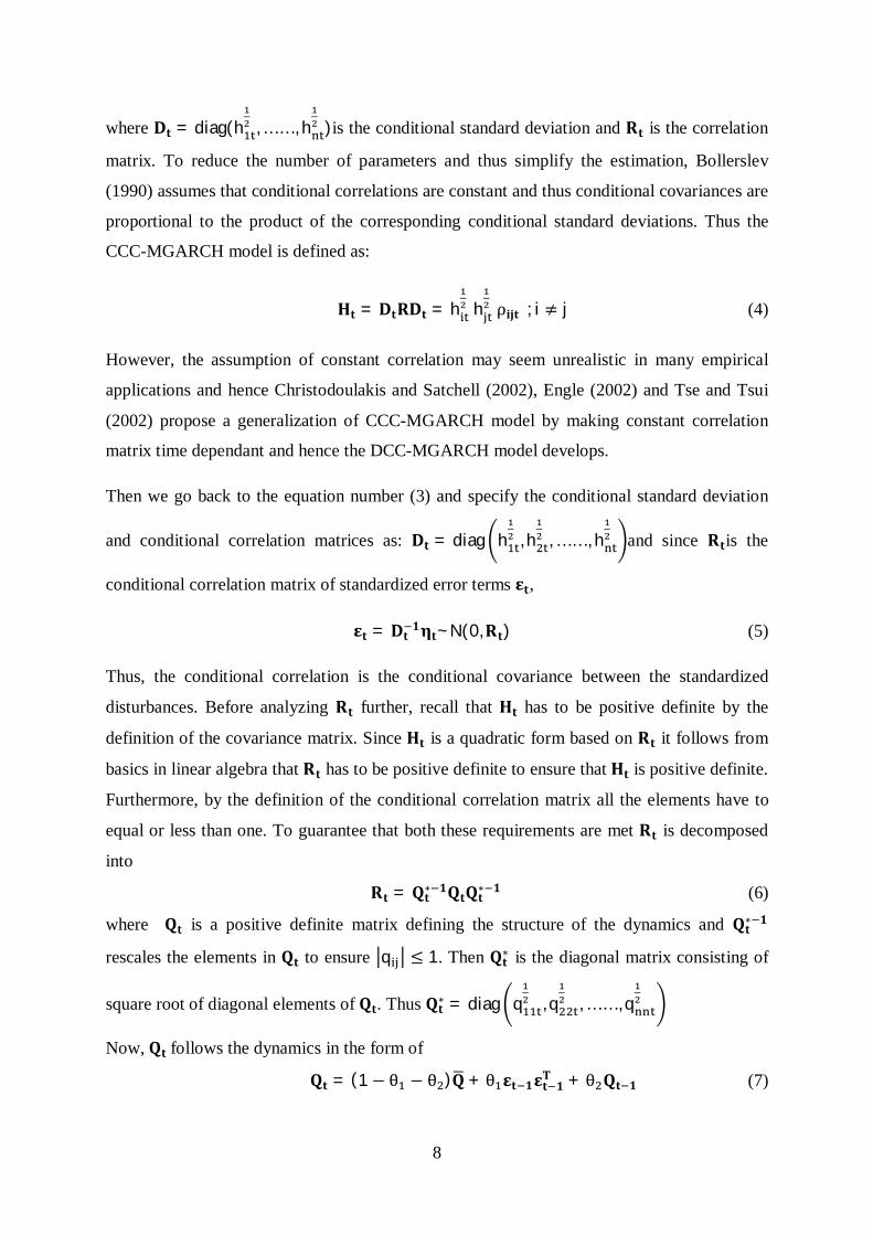
where 퐃퐭 = diag(h , … … , h )is the conditional standard deviation and 퐑퐭 is the correlation

matrix. To reduce the number of parameters and thus simplify the estimation, Bollerslev

(1990) assumes that conditional correlations are constant and thus conditional covariances are

proportional to the product of the corresponding conditional standard deviations. Thus the

CCC-MGARCH model is defined as:

퐇퐭 = 퐃퐭퐑퐃퐭 = h h ρ퐢퐣퐭; i ≠ j (4)

However, the assumption of constant correlation may seem unrealistic in many empirical

applications and hence Christodoulakis and Satchell (2002), Engle (2002) and Tse and Tsui

(2002) propose a generalization of CCC-MGARCH model by making constant correlation

matrix time dependant and hence the DCC-MGARCH model develops.

Then we go back to the equation number (3) and specify the conditional standard deviation

and conditional correlation matrices as: 퐃퐭 = diag h , h , … … , h and since 퐑퐭is the

conditional correlation matrix of standardized error terms 훆퐭,

훆퐭 = 퐃퐭ퟏ훈퐭~N(0,퐑퐭) (5)

Thus, the conditional correlation is the conditional covariance between the standardized

disturbances. Before analyzing 퐑퐭 further, recall that 퐇퐭 has to be positive definite by the

definition of the covariance matrix. Since 퐇퐭 is a quadratic form based on 퐑퐭 it follows from

basics in linear algebra that 퐑퐭 has to be positive definite to ensure that 퐇퐭 is positive definite.

Furthermore, by the definition of the conditional correlation matrix all the elements have to

equal or less than one. To guarantee that both these requirements are met 퐑퐭 is decomposed

into

퐑퐭 = 퐐퐭∗ ퟏ퐐퐭퐐퐭

∗ ퟏ (6)

where 퐐퐭 is a positive definite matrix defining the structure of the dynamics and 퐐퐭∗ ퟏ

rescales the elements in 퐐퐭 to ensure q ≤ 1. Then 퐐퐭∗ is the diagonal matrix consisting of

square root of diagonal elements of 퐐퐭. Thus 퐐퐭∗ = diag q , q , … … , q

Now, 퐐퐭follows the dynamics in the form of

퐐퐭 = (1 − θ − θ )퐐 + θ 훆퐭 ퟏ훆퐭 ퟏ퐓 + θ 퐐퐭 ퟏ (7)

9

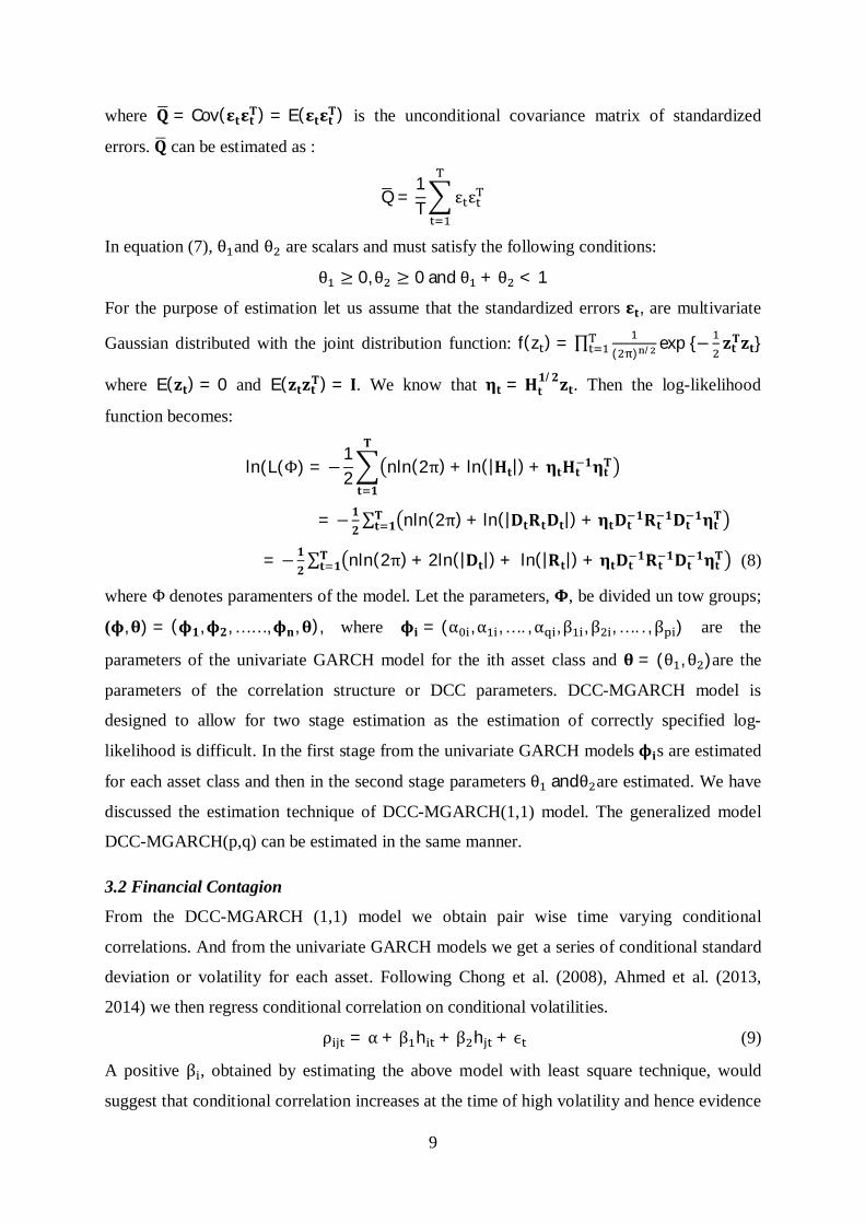
where 퐐 = Cov(훆퐭훆퐭퐓) = E(훆퐭훆퐭퐓) is the unconditional covariance matrix of standardized

errors. 퐐 can be estimated as :

Q =1T ε ε

In equation (7), θ and θ are scalars and must satisfy the following conditions:

θ ≥ 0,θ ≥ 0andθ + θ < 1

For the purpose of estimation let us assume that the standardized errors 훆퐭, are multivariate

Gaussian distributed with the joint distribution function: f(z ) = ∏( ) / exp{− 퐳퐭퐓퐳퐭}

where E(퐳퐭) = 0 and E(퐳퐭퐳퐭퐓) = 퐈. We know that 훈퐭 = 퐇퐭ퟏ/ퟐ퐳퐭. Then the log-likelihood

function becomes:

ln(L(Φ) = −12 nln(2π) + ln(|퐇퐭|) + 훈퐭퐇퐭

ퟏ훈퐭퐓퐓

퐭 ퟏ

= − ퟏퟐ∑ nln(2π) + ln(|퐃퐭퐑퐭퐃퐭|) + 훈퐭퐃퐭

ퟏ퐑퐭ퟏ퐃퐭

ퟏ훈퐭퐓퐓퐭 ퟏ

= − ퟏퟐ∑ nln(2π) + 2ln(|퐃퐭|) + ln(|퐑퐭|) + 훈퐭퐃퐭

ퟏ퐑퐭ퟏ퐃퐭

ퟏ훈퐭퐓퐓퐭 ퟏ (8)

where Φdenotes paramenters of the model. Let the parameters, 횽, be divided un tow groups;

(훟,훉) = (훟ퟏ,훟ퟐ, … … ,훟퐧,훉), where 훟퐢 = (α ,α , … . , α ,β , β , … . . , β ) are the

parameters of the univariate GARCH model for the ith asset class and 훉 = (θ , θ )are the

parameters of the correlation structure or DCC parameters. DCC-MGARCH model is

designed to allow for two stage estimation as the estimation of correctly specified log-

likelihood is difficult. In the first stage from the univariate GARCH models 훟퐢s are estimated

for each asset class and then in the second stage parameters θ andθ are estimated. We have

discussed the estimation technique of DCC-MGARCH(1,1) model. The generalized model

DCC-MGARCH(p,q) can be estimated in the same manner.

3.2 Financial Contagion

From the DCC-MGARCH (1,1) model we obtain pair wise time varying conditional

correlations. And from the univariate GARCH models we get a series of conditional standard

deviation or volatility for each asset. Following Chong et al. (2008), Ahmed et al. (2013,

2014) we then regress conditional correlation on conditional volatilities.

ρ = α + β h + β h + ϵ (9)

A positive β , obtained by estimating the above model with least square technique, would

suggest that conditional correlation increases at the time of high volatility and hence evidence

10

in favour of financial contagion. In case of multiple regressions, adjusted R2 or R measures

the goodness of fit. Here we can interpret the same as the degree of financial contagion.

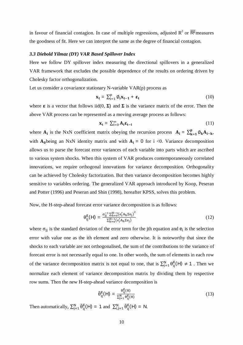
3.3 Diebold Yilmaz (DY) VAR Based Spillover Index

Here we follow DY spillover index measuring the directional spillovers in a generalized

VAR framework that excludes the possible dependence of the results on ordering driven by

Cholesky factor orthogonalization.

Let us consider a covariance stationary N-variable VAR(p) process as

퐱퐭 = ∑ ∅퐢퐱퐭 ퟏ + 훆퐭 (10)

where 훆 is a vector that follows iid(0, 횺) and 횺 is the variance matrix of the error. Then the

above VAR process can be represented as a moving average process as follows:

퐱퐭 = ∑ 퐀퐢훆퐭 퐢 (11)

where 퐀퐢 is the NxN coefficient matrix obeying the recursion process 퐀퐢 = ∑ ∅퐤퐀퐢 퐤퐩퐤 ퟏ ,

with 퐀ퟎbeing an NxN identity matrix and with 퐀퐢 = 0 for i <0. Variance decomposition

allows us to parse the forecast error variances of each variable into parts which are ascribed

to various system shocks. When this system of VAR produces contemporaneously correlated

innovations, we require orthogonal innovations for variance decomposition. Orthogonality

can be achieved by Cholesky factorization. But then variance decomposition becomes highly

sensitive to variables ordering. The generalized VAR approach introduced by Koop, Peseran

and Potter (1996) and Peseran and Shin (1998), hereafter KPSS, solves this problem.

Now, the H-step-ahead forecast error variance decomposition is as follows:

θ (H) =∑

∑ (12)

where σ is the standard deviation of the error term for the jth equation and e is the selection

error with value one as the ith element and zero otherwise. It is noteworthy that since the

shocks to each variable are not orthogonalised, the sum of the contributions to the variance of

forecast error is not necessarily equal to one. In other words, the sum of elements in each row

of the variance decomposition matrix is not equal to one, that is ∑ θ (H) ≠ 1 . Then we

normalize each element of variance decomposition matrix by dividing them by respective

row sums. Then the new H-step-ahead variance decomposition is

θ (H) =( )

∑ ( ) (13)

Then automatically, ∑ θ (H) = 1 and ∑ θ (H) = N, .

11

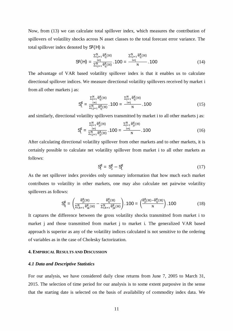
Now, from (13) we can calculate total spillover index, which measures the contribution of

spillovers of volatility shocks across N asset classes to the total forecast error variance. The

total spillover index denoted by S (H) is

S (H) =∑ ( ),

∑ ( ),. 100 =

∑ ( ),

. 100 (14)

The advantage of VAR based volatility spillover index is that it enables us to calculate

directional spillover indices. We measure directional volatility spillovers received by market i

from all other markets j as:

S . =∑ ( )

∑ ( ),. 100 =

∑ ( )

. 100 (15)

and similarly, directional volatility spillovers transmitted by market i to all other markets j as:

S . =∑ ( )

∑ ( ),. 100 =

∑ ( )

. 100 (16)

After calculating directional volatility spillover from other markets and to other markets, it is

certainly possible to calculate net volatility spillover from market i to all other markets as

follows:

S = S. − S . (17)

As the net spillover index provides only summary information that how much each market

contributes to volatility in other markets, one may also calculate net pairwise volatility

spillovers as follows:

S =( )

∑ ( ),−

( )

∑ ( ),. 100 =

( ) ( ). 100 (18)

It captures the difference between the gross volatility shocks transmitted from market i to

market j and those transmitted from market j to market i. The generalized VAR based

approach is superior as any of the volatility indices calculated is not sensitive to the ordering

of variables as in the case of Cholesky factorization.

4. EMPIRICAL RESULTS AND DISCUSSION

4.1 Data and Descriptive Statistics

For our analysis, we have considered daily close returns from June 7, 2005 to March 31,

2015. The selection of time period for our analysis is to some extent purposive in the sense

that the starting date is selected on the basis of availability of commodity index data. We

12

have used commodity index data from the database of Multi Commodity Exchange, India and

they started reporting commodity indices from June 7, 2005. In this analysis, we have also

used data of daily rupee/dollar exchange rate collected from Reserve Bank of India’s

database, daily data of gold price in India collected from World Gold Council database, daily

government securities index data constructed by National Stock Exchange, India and

SENSEX data of Bombay Stock Exchange (BSE). The period of time we choose for our

analysis allows us to investigate the sensitivity of commodity returns vis-à-vis returns of

other financial assets to the following major effects: the Subprime crisis of 2007-09,

Eurozone crisis of 2010-12, and large rupee depreciation of 2013-14.

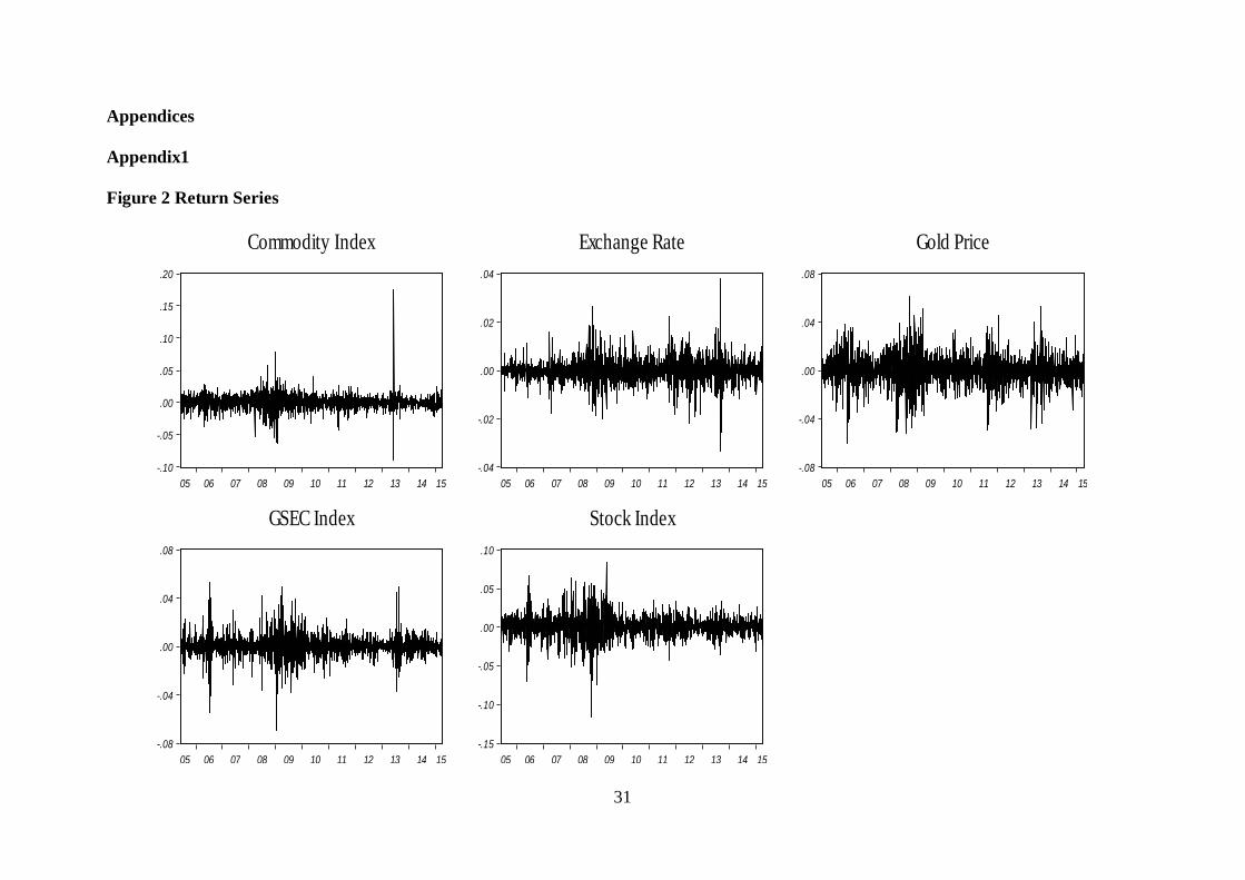
It is customary to calculate return of an asset as the logarithmic value of the ratio of two

consecutive prices (see Figure 2 in Appendix 1 for the graphical representation). More

precisely, the continuously compounded daily returns are computed using the following

logarithmic filter:

푟 , = 푙푛 ,

, (19)

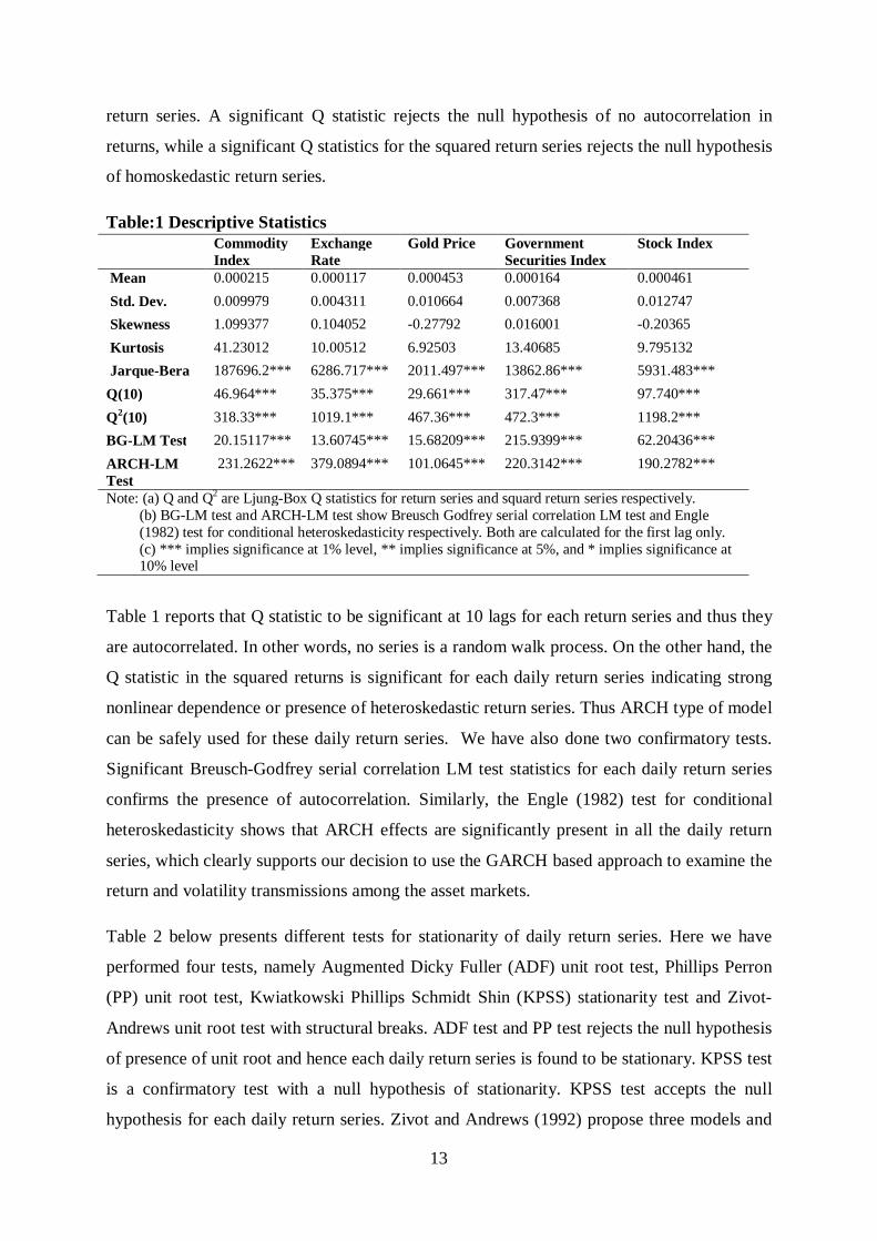
To have a gross idea of basic feature of data we should check the descriptive statistics for

each series. Table 1 below shows relevant descriptive statistics for each daily return series.

The data suggest that over the sample period, stock market offers highest average daily

returns (0.046%) and exchange rate arbitrage offers least reruns (0.012%). However, this

stock market is the most risky, as approximated by a standard deviation of 1.27% followed by

the gold market (1.07%) and commodity market (0.99%). This certainly gives indication

towards the conjecture that high uncertainty or risk is associated with high potential returns.

The commodity market offers medium return with a moderate risk; and hence investors can

use commodity as a “diversifier” in their portfolios. It is important to look into the skewness

coefficients to understand the nature of statistical distribution. Interestingly, commodity,

exchange rate and government securities returns are positively skewed, while gold and stock

returns show negatively skewed distribution. For all markets, kurtosis values are much higher

than that of a normal distribution implying significant departure from normal distribution.

This fact can be confirmed by the Jarque-Bera test with null hypothesis of normality

distributed returns. In all cases, the null hypothesis of is persuasively rejected. However, we

should remember that these facts are relevant only for the unconditional distributions of

return series. The Ljung-Box Q statistic test the null hypothesis of no serial correlation or no

autocorrelation and is calculated using upto 10 lags for both daily return series and squared

13

return series. A significant Q statistic rejects the null hypothesis of no autocorrelation in

returns, while a significant Q statistics for the squared return series rejects the null hypothesis

of homoskedastic return series.

Table:1 Descriptive Statistics Commodity

Index Exchange Rate

Gold Price Government Securities Index

Stock Index

Mean 0.000215 0.000117 0.000453 0.000164 0.000461 Std. Dev. 0.009979 0.004311 0.010664 0.007368 0.012747 Skewness 1.099377 0.104052 -0.27792 0.016001 -0.20365 Kurtosis 41.23012 10.00512 6.92503 13.40685 9.795132 Jarque-Bera 187696.2*** 6286.717*** 2011.497*** 13862.86*** 5931.483*** Q(10) 46.964*** 35.375*** 29.661*** 317.47*** 97.740*** Q2(10) 318.33*** 1019.1*** 467.36*** 472.3*** 1198.2*** BG-LM Test 20.15117*** 13.60745*** 15.68209*** 215.9399*** 62.20436*** ARCH-LM Test

231.2622*** 379.0894*** 101.0645*** 220.3142*** 190.2782***

Note: (a) Q and Q2 are Ljung-Box Q statistics for return series and squard return series respectively. (b) BG-LM test and ARCH-LM test show Breusch Godfrey serial correlation LM test and Engle (1982) test for conditional heteroskedasticity respectively. Both are calculated for the first lag only. (c) *** implies significance at 1% level, ** implies significance at 5%, and * implies significance at 10% level

Table 1 reports that Q statistic to be significant at 10 lags for each return series and thus they

are autocorrelated. In other words, no series is a random walk process. On the other hand, the

Q statistic in the squared returns is significant for each daily return series indicating strong

nonlinear dependence or presence of heteroskedastic return series. Thus ARCH type of model

can be safely used for these daily return series. We have also done two confirmatory tests.

Significant Breusch-Godfrey serial correlation LM test statistics for each daily return series

confirms the presence of autocorrelation. Similarly, the Engle (1982) test for conditional

heteroskedasticity shows that ARCH effects are significantly present in all the daily return

series, which clearly supports our decision to use the GARCH based approach to examine the

return and volatility transmissions among the asset markets.

Table 2 below presents different tests for stationarity of daily return series. Here we have

performed four tests, namely Augmented Dicky Fuller (ADF) unit root test, Phillips Perron

(PP) unit root test, Kwiatkowski Phillips Schmidt Shin (KPSS) stationarity test and Zivot-

Andrews unit root test with structural breaks. ADF test and PP test rejects the null hypothesis

of presence of unit root and hence each daily return series is found to be stationary. KPSS test

is a confirmatory test with a null hypothesis of stationarity. KPSS test accepts the null

hypothesis for each daily return series. Zivot and Andrews (1992) propose three models and

14

in all three models for testing unit root test, the null hypothesis is that the series contains a

unit root with a drift that excludes any structural break; and the alternative hypothesis is that

the series is a trend stationary process with a one-time break occurring at an unknown point

of time. Table 2 below shows that for each series, null hypothesis of presence of unit root is

rejected for Zivot Andrews test. It is interesting that except for the exchange rate, for all other

markets break dates fall in the interlude of financial crisis. For the exchange rate break date is

found on the date when rupee was at its pinnacle13.

Table:2 Unit root Tests ADF Test PP Test KPSS

Test Zivot Andrews Test

Commodity Index -39.928*** -51.0514***

0.084293 -40.32372*** (24th Dec, 2008)

Exchange Rate -51.8388***

-52.1147***

0.050696 -23.79214*** (29th Aug, 2013)

Gold Price -51.6235***

-51.5531***

0.0392 -51.67665*** (7th Jul, 2007)

Government Securities Index -29.9934***

-89.1908***

0.031967 -38.42199*** (7th Jan, 2009)

Stock Index -32.156*** -47.8907***

0.093062 -32.47446*** (21st Nov, 2008)

Note: (a) For ADF and Zivot Andrews tests standard t-statistics are reported. (b) For PP test adjusted t statistics are reported and significant statics are chosen on the basis of MacKinnon (1996) probability values. (c)For KPSS test, LM statistics are reported. (d)For Zivot Andrews test structural break points are given in parentheses. (e)*** implies significance at 1% level, ** implies significance at 5%, and * implies significance at 10%

level.

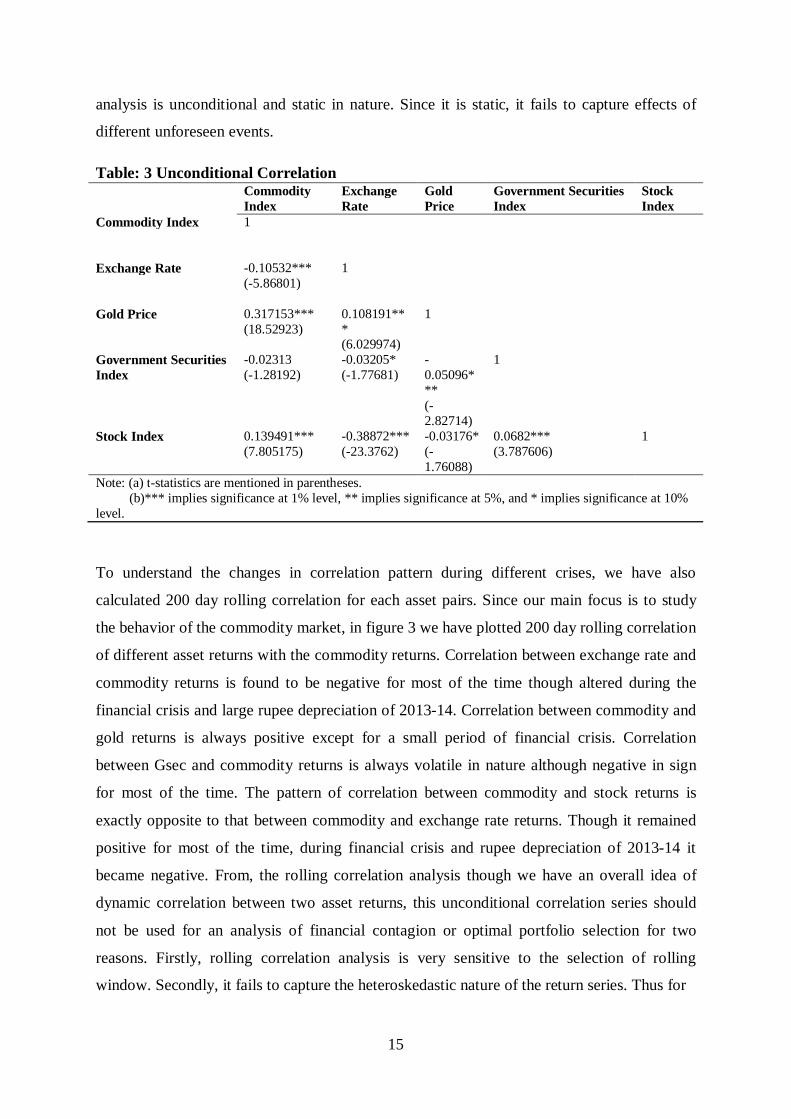
Table 3 below shows the unconditional correlation matrix. It is seen that commodity index is

relatively highly correlated with gold price and stock price. It is captivating to see that

commodity returns has a negative correlation with exchange rate and Gsec returns while it

has a positive correlation with gold price and stock price. Another interesting fact is that

though gold is also a type of commodity, it bears a negative correlation with stock returns.

This is true even when the correlation coefficients with exchange rate return are considered.

The stock return, on the other hand, is also highly negatively correlated with the exchange

rate returns. Gsec returns has a low correlation with all other assets returns, indicating that

government securities can be used as a “safe haven” in an asset portfolio. But this correlation

13 On August 28, 2013 Indian rupee experienced greatest fall and had gone down to 68.825 against the US dollar.

15

analysis is unconditional and static in nature. Since it is static, it fails to capture effects of

different unforeseen events.

Table: 3 Unconditional Correlation Commodity

Index Exchange Rate

Gold Price

Government Securities Index

Stock Index

Commodity Index 1

Exchange Rate -0.10532*** (-5.86801)

1

Gold Price 0.317153*** (18.52923)

0.108191*** (6.029974)

1

Government Securities Index

-0.02313 (-1.28192)

-0.03205* (-1.77681)

-0.05096*** (-2.82714)

1

Stock Index 0.139491*** (7.805175)

-0.38872*** (-23.3762)

-0.03176* (-1.76088)

0.0682*** (3.787606)

1

Note: (a) t-statistics are mentioned in parentheses. (b)*** implies significance at 1% level, ** implies significance at 5%, and * implies significance at 10%

level.

To understand the changes in correlation pattern during different crises, we have also

calculated 200 day rolling correlation for each asset pairs. Since our main focus is to study

the behavior of the commodity market, in figure 3 we have plotted 200 day rolling correlation

of different asset returns with the commodity returns. Correlation between exchange rate and

commodity returns is found to be negative for most of the time though altered during the

financial crisis and large rupee depreciation of 2013-14. Correlation between commodity and

gold returns is always positive except for a small period of financial crisis. Correlation

between Gsec and commodity returns is always volatile in nature although negative in sign

for most of the time. The pattern of correlation between commodity and stock returns is

exactly opposite to that between commodity and exchange rate returns. Though it remained

positive for most of the time, during financial crisis and rupee depreciation of 2013-14 it

became negative. From, the rolling correlation analysis though we have an overall idea of

dynamic correlation between two asset returns, this unconditional correlation series should

not be used for an analysis of financial contagion or optimal portfolio selection for two

reasons. Firstly, rolling correlation analysis is very sensitive to the selection of rolling

window. Secondly, it fails to capture the heteroskedastic nature of the return series. Thus for

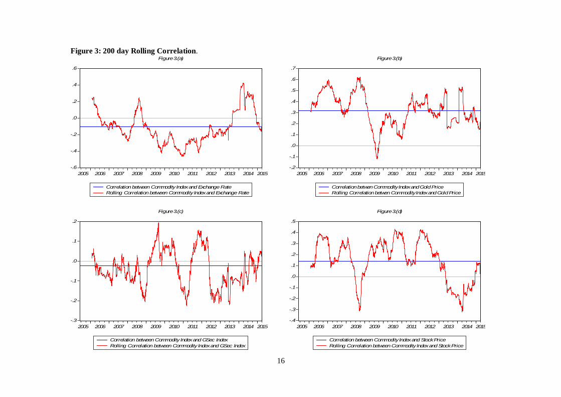
16

Figure 3: 200 day Rolling Correlation.

-.6

-.4

-.2

.0

.2

.4

.6

2005 2006 2007 2008 2009 2010 2011 2012 2013 2014 2015

Correlation between Commodity Index and Exchange RateRolling Correlation between Commodity Index and Exchange Rate

Figure 3.(a)

-.2

-.1

.0

.1

.2

.3

.4

.5

.6

.7

2005 2006 2007 2008 2009 2010 2011 2012 2013 2014 2015

Correlation betwen Commodity Index and Gold PriceRolling Correlation betwen Commodity Index and Gold Price

Figure 3.(b)

-.3

-.2

-.1

.0

.1

.2

2005 2006 2007 2008 2009 2010 2011 2012 2013 2014 2015

Correlation between Commodity Index and GSec IndexRolling Correlation between Commodity Index and GSec Index

Figure 3.(c)

-.4

-.3

-.2

-.1

.0

.1

.2

.3

.4

.5

2005 2006 2007 2008 2009 2010 2011 2012 2013 2014 2015

Correlation between Commodity Index and Stock PriceRolling Correlation between Commodity Index and Stock Price

Figure 3.(d)

17

our analysis of financial contagion we have decided to use conditional correlation series

obtained from MGARCH analysis.

4.2 Analysis of Dynamic Correlation and Financial Contagion

Table 4 below reports results of CCC-MGARCH and DCC-MGARCH models. The upper

part of the table shows univariate GARCH results for each daily return series. The two

coefficients of univariate GARCH models, namely α and β, are found to be significant for

each asset class. The sum of α and β implies the overall persistence of the series. Since for

every daily return series α and β are positive and (α + β) is found to be less than one, the

stability condition is said to be satisfied. A high and close to one value of (α + β) gives

evidence in favour of persistence of shocks or persistence of volatility, i.e. if any shock

appears in these markets, it takes longer time to die down. From the table it can also be seen

that two DCC parameters, and 2 are positive and significant; and ( + 2) is also found to

be less than one. Thus, the overall stability condition of DCC-MGARCH model is also

satisfied. Significance of DCC parameters implies a substantial time-varying co-movement.

In the lower part of the table conditional correlations of commodity index with other assets

are reported for both CCC-MGARCH and DCC-MGARCH models. For DCC-MGARCH

model, we have calculated mean conditional correlation of commodity return with other asset

returns and then mean tests are done to check whether average conditional correlation differs

from zero or not. Engle (2002) suggests that if average correlations are found to be zero from

the DCC-MGARCH model then it is meaningful to estimate CCC-MGARCH model. None of

the correlation is found to be zero and thus DCC-MGARCH is the appropriate model here. It

is interesting to note that correlation coefficients obtained from CCC-MARCH and DCC-

MGARCH models do not differ significantly in terms of magnitude and sign; and thus give

evidence in favour of flawless estimation of both models. Although conditional correlations

are higher than unconditional correlations, their sign remain unaltered.

In the literature, contagion is defined as significant increases in cross market correlations

during the turmoil period, while any continued increase in cross market correlation at high

levels is referred as interdependence. This is mainly because it is assumed that if there is a

significant increase in correlation, there is a strengthening of transmission mechanisms

between the two markets under consideration (see Collins and Biekpe, 2003; Forbes and

Rigobon, 2002). To confirm this, we now analyze the estimated dynamic conditional

correlation. Conditional correlations (both constant and dynamic) are shown in figure 3.

18

Table: 4 CCC-MGARCH and DCC-MGARCH results with average Correlations. CCC-MGARCH DCC-MGARCH Commodity

Index Exchange Rate

Gold Price Government Security Index

Stock Index Commodity Index

Exchange Rate

Gold Price Government Security Index

Stock Index

μ 5.39E-05 (0.412845)

-9.11E-06 (-0.152024)

0.000265* (1.6769)

0.00033*** (4.21986)

0.000845*** (5.550561)

4.03E-05 (0.217836)

1.41E-05 (0.249608)

0.000338** (2.140407)

0.000323*** (3.158759)

0.000815*** (4.595350)

ω 8.57E-07*** (5.885968)

2.45E-07*** (10.05371)

8.87E-07*** (6.65504)

1.20E-06*** (11.61662)

1.94E-06*** (7.697098)

8.19E-07*** (3.620011)

2.21E-07*** (3.141093)

9.16E-07** (2.034635)

1.19E-06*** (3.768450)

1.88E-06*** (3.229232)

α 0.058748*** (22.29055)

0.071123*** (14.54964)

0.041851*** (12.38704)

0.187062*** (22.52277)

0.074442*** (14.21827)

0.060934*** (3.536532)

0.082989*** (6.683661)

0.047413*** (4.397705)

0.187538*** (6.877660)

0.082431*** (6.278558)

β 0.934096*** (282.5845)

0.915872*** (174.6334)

0.950232*** (265.7461)

0.81164*** (147.2014)

0.911657*** (163.3532)

0.932845*** (56.65161)

0.908127*** (73.61097)

0.944886*** (72.46170)

0.811340*** (32.35832)

0.905511*** (64.32363)

α+β 0.992844 0.986995 0.992083 0.998702 0.986099 0.993779 0.991116 0.992299 0.998923 0.987942 0.015620***

(6.558015) 0.951165***

(93.95479) Corr(Commodity Index, Exchange Rate)

-0.12348*** (-8.04712)

-0.123624*** (-80.49825)

Corr(Commodity Index, Gold Price)

0.332613*** (24.26903)

0.332567*** (266.6531)

Corr(Commodity Index, Government Security Index)

-0.04255*** (-2.57834)

-0.042285*** (-40.38605)

Corr(Commodity Index, Spot Index)

0.133969*** (8.524783)

0.135749*** (92.76282)

Note: (a) z-statistics are mentioned in parentheses. For correlations of DCC model t-statistics are mentioned in parentheses. (b)*** implies significance at 1% level, ** implies significance at 5%, and * implies significance at 10% level.

19

Figure 4: Constant and Dynamic Conditional Correlations

-.4

-.3

-.2

-.1

.0

.1

.2

2005 2006 2007 2008 2009 2010 2011 2012 2013 2014 2015

CCC between Commodity Index and Exchange RateDCC between Commodity Index and Exchange Rate

Figure 4.(a)

.0

.1

.2

.3

.4

.5

.6

2005 2006 2007 2008 2009 2010 2011 2012 2013 2014 2015

CCC between Commodity Index and Gold PriceDCC between Commodity Index and Gold Price

Figure 4.(b)

-.3

-.2

-.1

.0

.1

.2

2005 2006 2007 2008 2009 2010 2011 2012 2013 2014 2015

CCC between Commodity Index and GSec IndexDCC between Commodity Index and Gsec Index

Figure. 4(c)

-.2

-.1

.0

.1

.2

.3

.4

2005 2006 2007 2008 2009 2010 2011 2012 2013 2014 2015

CCC between Commodity Index and Stock IndexDCC between Commodity Index and Stock Index

Figure 4.(d)

20

The overall trend of conditional correlations does not differ significantly from that of the

unconditional correlation. However, in many cases unconditional correlation fails to capture

significant market movements and in some other cases it overestimates correlation and thus

overemphasizes significance of some shocks.

For example, if we notice the dynamic correlation between commodity index and exchange

rate (in figure 4.(a)), we find similarity with the unconditional (rolling) correlation. However,

in unconditional case, as heteroskedasticity is pushed aside, correlation is overestimated

especially during financial crisis of 2007-09 and rupee depreciation of 2013-14. The

correlation between the two touched its lowest value in the mid 2013 and this incident was

not unveiled from the unconditional correlation. Similarly, while studying conditional

correlation between commodity index and gold price (see figure 4.(b)), we notice a huge ups

and downs in 2013. Even this phenomenon was not revealed from the unconditional

correlation. The correlation between the two prior to the financial crisis, was overestimated in

the case of unconditional correlation. So is the case for correlation between commodity index

and stock price in 2013-14. The reason behind this imprecise exploration of market co-

movements is ignorance of heteroskedasticity and conditional behavior of the daily return

series. When a series is conditional upon its past value, it evidently captures all information

available till that time period; and hence it is appropriate to consider conditional correlation

for the analysis of financial contagion or optimal portfolio selection.

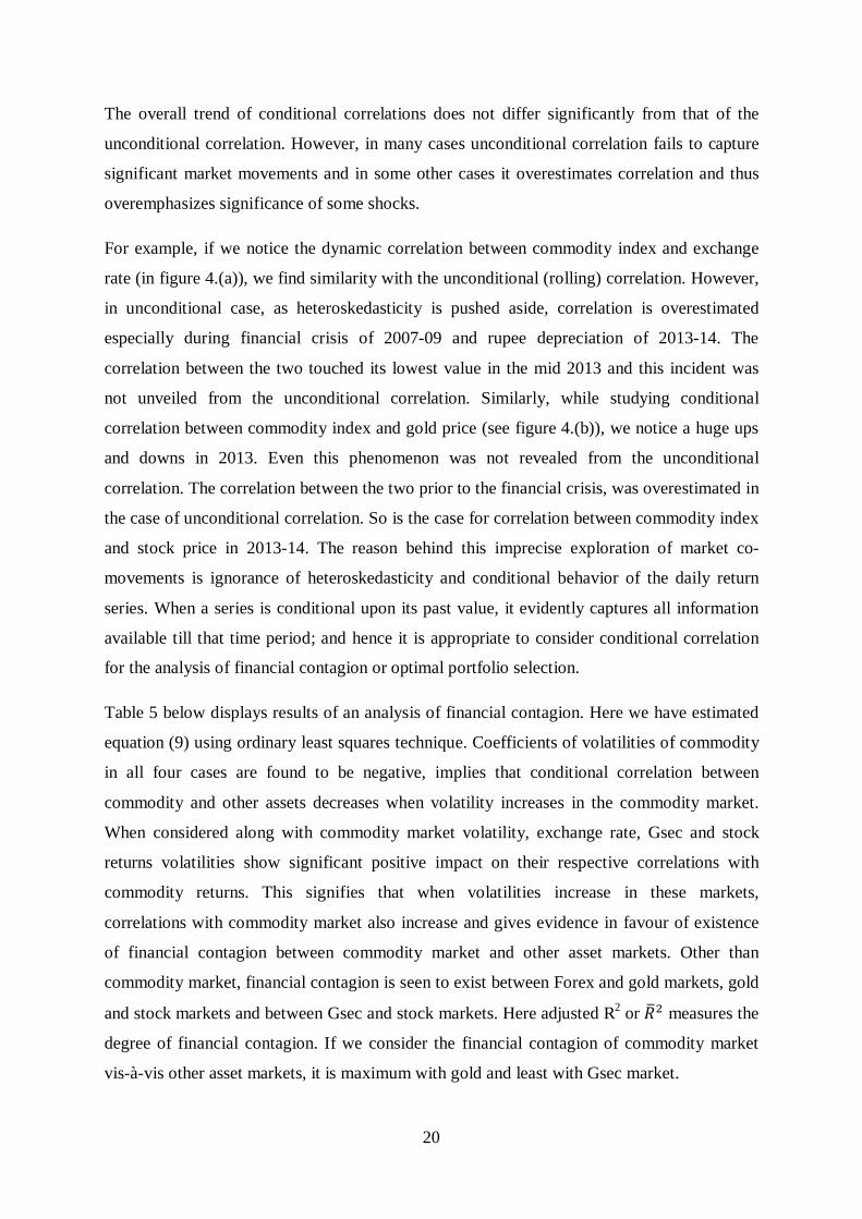
Table 5 below displays results of an analysis of financial contagion. Here we have estimated

equation (9) using ordinary least squares technique. Coefficients of volatilities of commodity

in all four cases are found to be negative, implies that conditional correlation between

commodity and other assets decreases when volatility increases in the commodity market.

When considered along with commodity market volatility, exchange rate, Gsec and stock

returns volatilities show significant positive impact on their respective correlations with

commodity returns. This signifies that when volatilities increase in these markets,

correlations with commodity market also increase and gives evidence in favour of existence

of financial contagion between commodity market and other asset markets. Other than

commodity market, financial contagion is seen to exist between Forex and gold markets, gold

and stock markets and between Gsec and stock markets. Here adjusted R2 or 푅 measures the

degree of financial contagion. If we consider the financial contagion of commodity market

vis-à-vis other asset markets, it is maximum with gold and least with Gsec market.

21

Table:5 Existence and Extent of Financial Contagion Constant hi hj 푹ퟐ Commodity Index--Exchange Rate -0.10389***

(-23.4061)

-2.89009*** (-7.58788)

1.68713* (1.772027)

0.018096

Commodity Index--Gold Price 0.307556*** (82.23817)

-5.42061*** (-16.1191)

7.371216*** (17.57908)

0.105327

Commodity Index--Government Security Index -0.03878*** (-14.3265)

-0.78929*** (-3.01081)

0.554739* (1.905327)

0.003193

Commodity Index-- Stock Index 0.13161*** (34.81747)

-3.54792*** (-9.08991)

3.19809*** (10.50074)

0.039686

Exchange Rate--Gold Price 0.004291 (1.114111)

8.40891*** (10.94734)

2.61516*** (6.825251)

0.088954

Exchange rate--Government security Index 5.39E-05 (0.020323)

-1.24489** (-2.18553)

-0.26431 (-1.04439)

0.001818

Exchange Rate--Stock Index -0.32353*** (-106.339)

-11.9391*** (-18.4748)

-1.09063*** (-5.40649)

0.137271

Gold Price--Government Security Index 0.023325*** (7.694132)

-3.1611*** (-11.1614)

-0.71761*** (-2.84467)

0.050364

Gold Price--Stock Index -0.00048 (-0.10891)

-3.35088*** (-6.20017)

7.13E-01** (2.107381)

0.013707

Government Security Index--Stock Index 0.008113*** (3.01803)

2.365752*** (7.797846)

1.57747*** (7.400784)

0.059226

Note: (a) t-statistics are mentioned in parentheses. (b)*** implies significance at 1% level, ** implies significance at 5%, and * implies significance at 10% level.

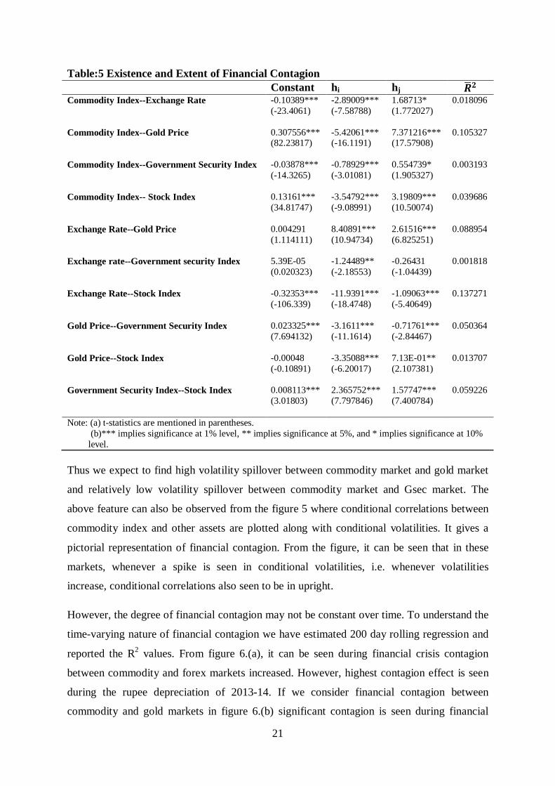
Thus we expect to find high volatility spillover between commodity market and gold market

and relatively low volatility spillover between commodity market and Gsec market. The

above feature can also be observed from the figure 5 where conditional correlations between

commodity index and other assets are plotted along with conditional volatilities. It gives a

pictorial representation of financial contagion. From the figure, it can be seen that in these

markets, whenever a spike is seen in conditional volatilities, i.e. whenever volatilities

increase, conditional correlations also seen to be in upright.

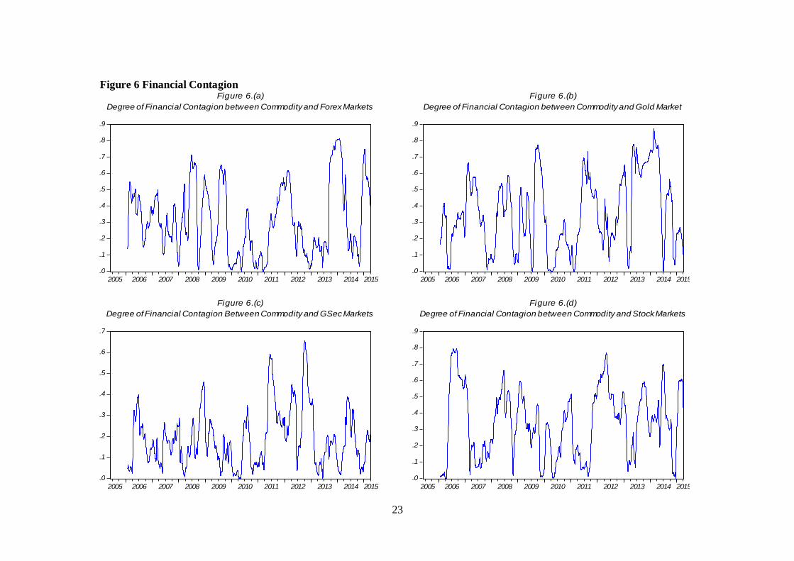
However, the degree of financial contagion may not be constant over time. To understand the

time-varying nature of financial contagion we have estimated 200 day rolling regression and

reported the R2 values. From figure 6.(a), it can be seen during financial crisis contagion

between commodity and forex markets increased. However, highest contagion effect is seen

during the rupee depreciation of 2013-14. If we consider financial contagion between

commodity and gold markets in figure 6.(b) significant contagion is seen during financial

22

Figure 5: Conditional Volatility and Conditional Correlation

-.4

-.3

-.2

-.1

.0

.1

.2.00

.01

.02

.03

.04

.05

.06

2005 2006 2007 2008 2009 2010 2011 2012 2013 2014 2015

Conditional SD (Commodity Index)Conditional SD (Exchange Rate)Conditional Correlation (Commodity Index, Exchange Rate)

Figure 5.(a)

.0

.1

.2

.3

.4

.5

.6

.00

.01

.02

.03

.04

.05

.06

2005 2006 2007 2008 2009 2010 2011 2012 2013 2014 2015

Conditional SD (Commodity Index)Conditional SD (Gold Price)Conditional Correlation (Commodity Index, Gold Price)

Figure 5.(b)

-.3

-.2

-.1

.0

.1

.2.00

.01

.02

.03

.04

.05

.06

2005 2006 2007 2008 2009 2010 2011 2012 2013 2014 2015

Conditional SD (Commodity Index)Conditional SD (Gsec Index)Conditioanl Correlation (Commodity Index , Gsec Index)

Figure 5.(c)

-.2

-.1

.0

.1

.2

.3

.4

.00

.01

.02

.03

.04

.05

.06

2005 2006 2007 2008 2009 2010 2011 2012 2013 2014 2015

Conditional SD (Commodity Index)Conditional SD (Stock Index)Conditioanl Correlation (Commodity Index, Stock Index)

Figure 5.(d)

23

Figure 6 Financial Contagion

.0

.1

.2

.3

.4

.5

.6

.7

.8

.9

2005 2006 2007 2008 2009 2010 2011 2012 2013 2014 2015

Figure 6.(a)Degree of Financial Contagion between Commodity and Forex Markets

.0

.1

.2

.3

.4

.5

.6

.7

.8

.9

2005 2006 2007 2008 2009 2010 2011 2012 2013 2014 2015

Figure 6.(b)Degree of Financial Contagion between Commodity and Gold Market

.0

.1

.2

.3

.4

.5

.6

.7

2005 2006 2007 2008 2009 2010 2011 2012 2013 2014 2015

Figure 6.(c)Degree of Financial Contagion Between Commodity and GSec Markets

.0

.1

.2

.3

.4

.5

.6

.7

.8

.9

2005 2006 2007 2008 2009 2010 2011 2012 2013 2014 2015

Figure 6.(d)Degree of Financial Contagion between Commodity and Stock Markets

24

crisis, second phase of Eurozone crisis and then during the period of large rupee depreciation.

However, the contagion between commodity and Gsec markets was not high during the

financial crisis as was seen for other markets (see figure 6.(c)). The contagion between these

two markets was mostly seen during the Eurozone crisis. Lastly, in figure 6.(d) we show

contagion between commodity and stock markets. It was significantly high throughout the

period of study except for the interim period of 2010-11. Thus we have found significant

financial contagion between commodity market and other asset markets especially during two

crises and period of large rupee depreciation. Here we should put a caveat that this dynamic

analysis of financial contagion is sensitive to the selection of rolling window. However, there

is no other technique available to check the extent of financial contagion considering

conditional volatilities and conditional correlations.

4.3 Analysis of Volatility Spillover

4.3.1 Unconditional Patterns: the Full Sample Volatility Spillover Analysis

Table 6 below shows the volatility spillovers among different asset markets. We have

calculated forecast error variance and hence volatility spillover indices on the basis of VAR

of order 2 and generalized variance decomposition of 10 day ahead volatility forecast

errors14. In the table, jth entry is the estimated contributions to the forecast error variance of

market i coming from innovations to market j. The off diagonal column sums (labeled

contributions TO others) and row sums (labeled contributions FROM others) are the total

volatility spillovers measured from ith market to all other markets and total volatility

spillovers measured from all other markets to ith market respectively. Net volatility spillovers

are calculated simply by subtracting “FROM spillover” from “To spillover”. It measures total

contributions of ith market in the total volatility spillover. Total spillover index is also shown

in the table. It is approximately the grand off diagonal column sum (or grand off diagonal

row sum) relative to the grand column sum including diagonals (or row sum including

diagonals), expressed as a percentage. Thus an approximate “input-output” decomposition of

the total volatility spillover index is shown in the volatility spillover table. The row labeled

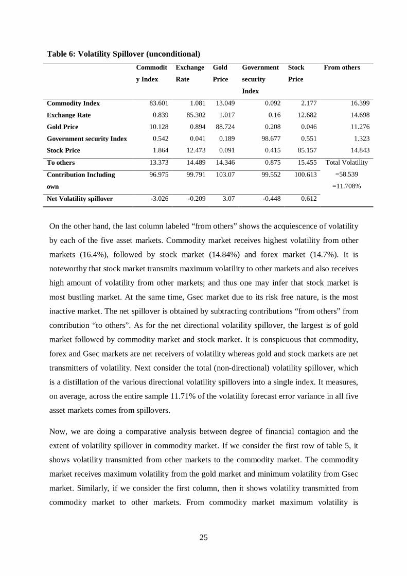
“to others”, shows the gross directional volatility spillovers to other markets from each of the

five asset markets. Transmission of volatility is highest for stock market (15.45%) followed

by forex market (14.49%) and Gold market (14.35%).

14 Optimal lag of VAR is selected on the basis of Schwarz Information Criterion (SIC).

25

Table 6: Volatility Spillover (unconditional) Commodit

y Index

Exchange

Rate

Gold

Price

Government

security

Index

Stock

Price

From others

Commodity Index 83.601 1.081 13.049 0.092 2.177 16.399

Exchange Rate 0.839 85.302 1.017 0.16 12.682 14.698

Gold Price 10.128 0.894 88.724 0.208 0.046 11.276

Government security Index 0.542 0.041 0.189 98.677 0.551 1.323

Stock Price 1.864 12.473 0.091 0.415 85.157 14.843

To others 13.373 14.489 14.346 0.875 15.455 Total Volatility

=58.539

=11.708%

Contribution Including

own

96.975 99.791 103.07 99.552 100.613

Net Volatility spillover -3.026 -0.209 3.07 -0.448 0.612

On the other hand, the last column labeled “from others” shows the acquiescence of volatility

by each of the five asset markets. Commodity market receives highest volatility from other

markets (16.4%), followed by stock market (14.84%) and forex market (14.7%). It is

noteworthy that stock market transmits maximum volatility to other markets and also receives

high amount of volatility from other markets; and thus one may infer that stock market is

most bustling market. At the same time, Gsec market due to its risk free nature, is the most

inactive market. The net spillover is obtained by subtracting contributions “from others” from

contribution “to others”. As for the net directional volatility spillover, the largest is of gold

market followed by commodity market and stock market. It is conspicuous that commodity,

forex and Gsec markets are net receivers of volatility whereas gold and stock markets are net

transmitters of volatility. Next consider the total (non-directional) volatility spillover, which

is a distillation of the various directional volatility spillovers into a single index. It measures,

on average, across the entire sample 11.71% of the volatility forecast error variance in all five

asset markets comes from spillovers.

Now, we are doing a comparative analysis between degree of financial contagion and the

extent of volatility spillover in commodity market. If we consider the first row of table 5, it

shows volatility transmitted from other markets to the commodity market. The commodity

market receives maximum volatility from the gold market and minimum volatility from Gsec

market. Similarly, if we consider the first column, then it shows volatility transmitted from

commodity market to other markets. From commodity market maximum volatility is

26

dispatched to the gold market and least to the Gsec market. This information is taken in

column 3 and 4 in table 6 below and also the total spillovers are calculated in column 5.

Table:6 Financial Contagion and Volatility Spillover, a Comparison

Degree of Financial Contagion

Rank

Volatility Spillover from i to j

Volatility Spillover from j to i

Total Volatility Spillover Between i and j

Rank

(1) (2) (3) (4) (5) (6)

Commodity Index--Exchange Rate

1.8096% 3 0.839% 1.081% 1.92% 3

Commodity Index--Gold Price

10.5327% 1 10.128% 13.049% 23.177% 1

Commodity Index--Government Security Index

0.3193% 4 0.542% 0.092% 0.634% 4

Commodity Index-- Stock Index

3.9686% 2 1.864% 2.177% 4.041% 2

Note: (a) Degrees of financial contagion, which is adjusted R2 expressed as percentages, are taken from table 5. (b) Volatility Spillover estimates in row 3 and 4 are taken from the first column and first row, respectively, of table 6. (c) Total volatility spillover is the sum of digits in column 3 and 4. (d) Ranks in column 2 and column 6 are on the basis of column 1 and column 5 respectively

It can be seen that the ranking on the basis of degree of financial contagion certainly matches

with the ranking of total volatility spillover; and hence more the degree of financial contagion

more is the evidence of volatility spillover.

4.3.2 Conditional and Dynamic Spillover analysis

Since our sample period includes some phases of financial market evolution and turbulence,

it seems unrealistic that any single fixed parameter model would apply over the entire

sample. Though the full sample spillover table and spillover index calculated earlier provides

a summary of the “average” volatility spillover behavior of the five markets, it certainly

misses out the important secular and cyclical movements in spillovers. To address this issue,

we now estimate volatility spillovers using 200-day rolling samples, and assess the extent and

nature of the spillover variation over time via the corresponding time series of spillover

indices, which we examine graphically in the figure 7 below.

27

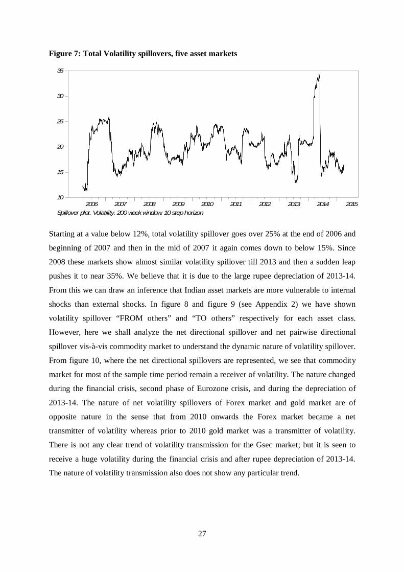
Figure 7: Total Volatility spillovers, five asset markets

Starting at a value below 12%, total volatility spillover goes over 25% at the end of 2006 and

beginning of 2007 and then in the mid of 2007 it again comes down to below 15%. Since

2008 these markets show almost similar volatility spillover till 2013 and then a sudden leap

pushes it to near 35%. We believe that it is due to the large rupee depreciation of 2013-14.

From this we can draw an inference that Indian asset markets are more vulnerable to internal

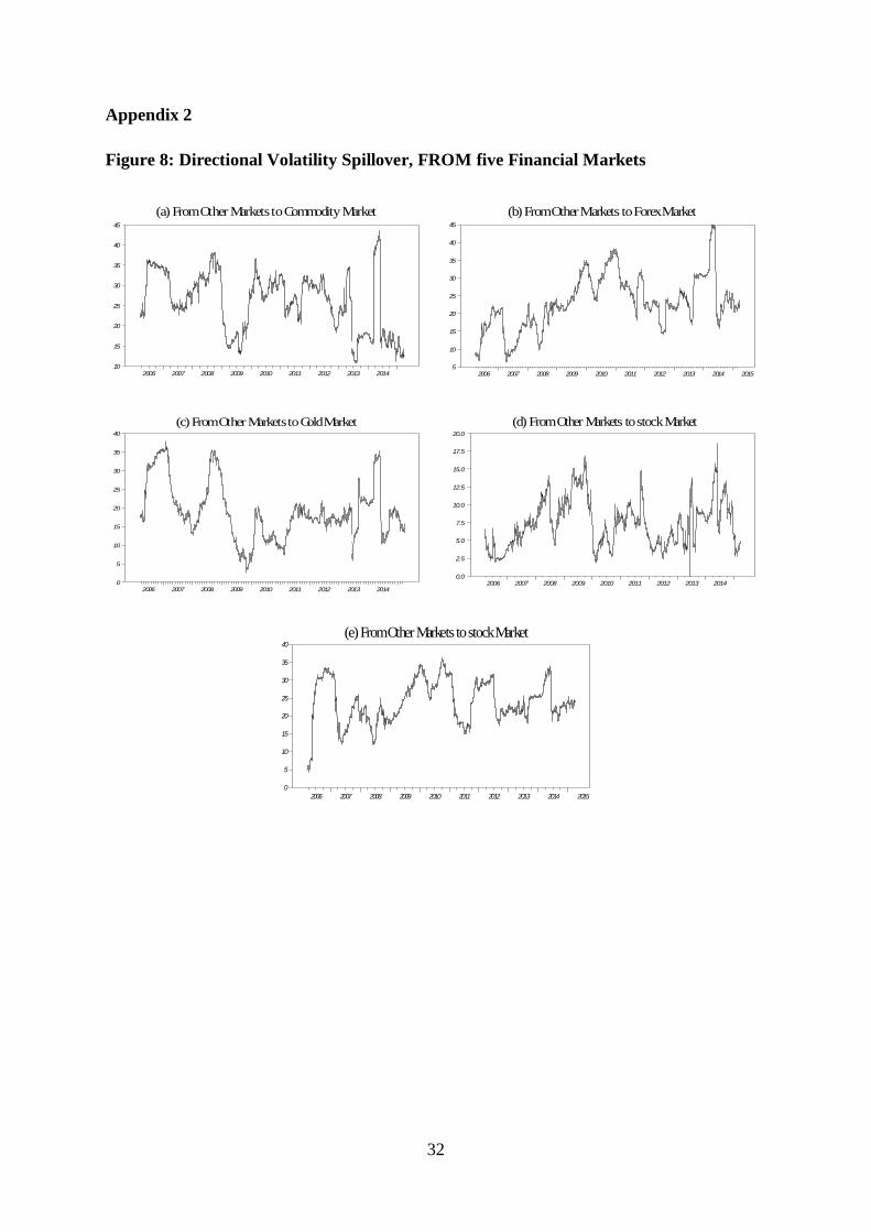
shocks than external shocks. In figure 8 and figure 9 (see Appendix 2) we have shown

volatility spillover “FROM others” and “TO others” respectively for each asset class.

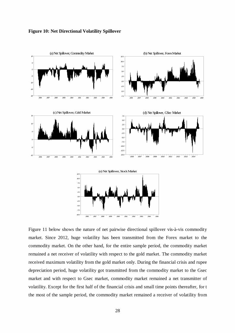
However, here we shall analyze the net directional spillover and net pairwise directional

spillover vis-à-vis commodity market to understand the dynamic nature of volatility spillover.

From figure 10, where the net directional spillovers are represented, we see that commodity

market for most of the sample time period remain a receiver of volatility. The nature changed

during the financial crisis, second phase of Eurozone crisis, and during the depreciation of

2013-14. The nature of net volatility spillovers of Forex market and gold market are of

opposite nature in the sense that from 2010 onwards the Forex market became a net

transmitter of volatility whereas prior to 2010 gold market was a transmitter of volatility.

There is not any clear trend of volatility transmission for the Gsec market; but it is seen to

receive a huge volatility during the financial crisis and after rupee depreciation of 2013-14.

The nature of volatility transmission also does not show any particular trend.

Spillover plot. Volatility. 200 week window. 10 step horizon2006 2007 2008 2009 2010 2011 2012 2013 2014 2015

10

15

20

25

30

35

28

Figure 10: Net Directional Volatility Spillover

Figure 11 below shows the nature of net pairwise directional spillover vis-à-vis commodity

market. Since 2012, huge volatility has been transmitted from the Forex market to the

commodity market. On the other hand, for the entire sample period, the commodity market

remained a net receiver of volatility with respect to the gold market. The commodity market

received maximum volatility from the gold market only. During the financial crisis and rupee

depreciation period, huge volatility got transmitted from the commodity market to the Gsec

market and with respect to Gsec market, commodity market remained a net transmitter of

volatility. Except for the first half of the financial crisis and small time points thereafter, for t

the most of the sample period, the commodity market remained a receiver of volatility from

(b) Net Spillover, Forex Market

2006 2007 2008 2009 2010 2011 2012 2013 2014 2015-7.5

-5.0

-2.5

0.0

2.5

5.0

7.5

10.0

12.5

(d) Net Spillover, GSec Market

2006 2007 2008 2009 2010 2011 2012 2013 2014-15.0

-12.5

-10.0

-7.5

-5.0

-2.5

0.0

2.5

5.0

7.5

(e) Net Spillover, Stock Market

2006 2007 2008 2009 2010 2011 2012 2013 2014 2015-10.0

-7.5

-5.0

-2.5

0.0

2.5

5.0

7.5

10.0

12.5

(a) Net Spillover, Commodity Market

2006 2007 2008 2009 2010 2011 2012 2013 2014 2015-20

-15

-10

-5

0

5

10

(c) Net Spillover, Gold Market

2006 2007 2008 2009 2010 2011 2012 2013 2014 2015-10

-5

0

5

10

15

29

Figure 11: Net Directional Volatility Spillover

(b) Net spillover Between Commodity Market and Gold Market

2006 2007 2008 2009 2010 2011 2012 2013 2014 2015-10

-8

-6

-4

-2

0

2

(d) Net Spillover Between Commodity Market and Stock market

2006 2007 2008 2009 2010 2011 2012 2013 2014 2015-5

-4

-3

-2

-1

0

1

2

3

4

(a) Net spillover Between Commodity Market and Forex Market

2006 2007 2008 2009 2010 2011 2012 2013 2014 2015-7.5

-5.0

-2.5

0.0

2.5

5.0

(c) Net Spillover Between Commodity Market and GSec Market

2006 2007 2008 2009 2010 2011 2012 2013 2014 2015-5.0

-2.5

0.0

2.5

5.0

7.5

10.0

30

the stock market. The extent of volatility spillover between the stock market and the

commodity market is seen to significantly decrease after 2010. This just the opposite for the

Forex market as the volatility spillover is seen to increase in magnitude after 2012. Thus we

can safely conclude that the commodity market, on an overall basis, is a receiver of volatility

from other markets.

5. CONCLUSION

Considering commodity as an asset class, we have estimated extent of financial contagion in

Indian asset markets. Commodity market is found to have significant contagion with other

asset markets. When the Indian commodity market is found to be most contagious to Indian

gold market, it is least contagious to Gsec market. In this study, we have investigated the

dynamic correlations between commodity, currency, gold, Gsec and stock returns as the

degree of financial contagion dependence on the dynamic conditional correlation between

two asset returns, and hence its nature changes over time. During financial crisis, Eurozone

crisis and mostly at the time of rupee depreciation, contagion of Indian commodity market is

seen to increase with other asset markets. Correlation between two asset returns and hence

extent of contagion between two asset markets play an important role in the process of

optimal portfolio selection. The dynamic correlation analysis infers, except for the crises

periods, commodities can be considered as hedge against exchange rate and Gsec; and as a

diversifier in the presence of gold and stocks. Markets are called “safe haven” if they provide

protection for each other during high volatilities. From our analysis it is evident that

commodities should not be treated as a “safe haven” when the portfolio consists of gold and

foreign currency. This conclusion has been strengthened by our analysis of volatility

spillover. We have found that firstly, the commodity market is a net receiver of volatility

from Forex, gold and stock markets. Secondly, the volatility transmission increases during

the period of stress. We have also done a comparative analysis between financial contagion

and volatility spillover to check whether there is any one to one connection. We see that for

the commodity market a high degree of financial contagion leads to higher volatility spillover

and vice versa. Our results have serious implications for optimal portfolio selection especially

when commodity is held as an asset in portfolio.

31

Appendices

Appendix1

Figure 2 Return Series

-.10

-.05

.00

.05

.10

.15

.20

05 06 07 08 09 10 11 12 13 14 15

Commodity Index

-.04

-.02

.00

.02

.04

05 06 07 08 09 10 11 12 13 14 15

Exchange Rate

-.08

-.04

.00

.04

.08

05 06 07 08 09 10 11 12 13 14 15

Gold Price

-.08

-.04

.00

.04

.08

05 06 07 08 09 10 11 12 13 14 15

GSEC Index

-.15

-.10

-.05

.00

.05

.10

05 06 07 08 09 10 11 12 13 14 15

Stock Index

32

Appendix 2

Figure 8: Directional Volatility Spillover, FROM five Financial Markets

(b) From Other Markets to Forex Market

2006 2007 2008 2009 2010 2011 2012 2013 2014 20155

10

15

20

25

30

35

40

45

(d) From Other Markets to stock Market

2006 2007 2008 2009 2010 2011 2012 2013 20140.0

2.5

5.0

7.5

10.0

12.5

15.0

17.5

20.0

(e) From Other Markets to stock Market

2006 2007 2008 2009 2010 2011 2012 2013 2014 20150

5

10

15

20

25

30

35

40

(a) From Other Markets to Commodity Market

2006 2007 2008 2009 2010 2011 2012 2013 201410

15

20

25

30

35

40

45

(c) From Other Markets to Gold Market

2006 2007 2008 2009 2010 2011 2012 2013 20140

5

10

15

20

25

30

35

40

33

Figure 9: Directional Volatility Spillover, TO five Financial Markets

(b) From Forex Market To Other Markets

2006 2007 2008 2009 2010 2011 2012 2013 2014 20150

10

20

30

40

50

60

(d) From Gsec Market To Other Markets

2006 2007 2008 2009 2010 2011 2012 2013 2014 20150

2

4

6

8

10

12

14

(e) From Stock Market To Other Markets

2006 2007 2008 2009 2010 2011 2012 2013 2014 20155

10

15

20

25

30

35

40

(a) From Commodity Market To Other Markets

2006 2007 2008 2009 2010 2011 2012 2013 2014 20155

10

15

20

25

30

35

40

45

(c) From Gold Market To Other Markets

2006 2007 2008 2009 2010 2011 2012 2013 2014 20155

10

15

20

25

30

35

40

45

50

34

REFERENCES

Acharya, V, and Pedersen, L. H. (2005). Asset Pricing with Liquidity Risk, Journal of Financial Economics 77(2), 375–410.

Ahmed, W, Seghal, S. and Bhanumurthy, N.R. (2013). Eurozone crisis and BRIICKS stock markets: contagion or market interdependence .Economic Modelling. 33, 209-225.

Ahmed, W., Seghal, S. and Bhanumurthy, N. R. (2014). The Eurozone crisis and its contagion effects on the European stock markets. Studies in Economics and Finance. 31 (3), 325-352.

Allen, F and Gale, D. . (2004). Financial Intermediaries and Markets.Econometrica. 72 (4), 1023–1061.

Aloui, R., Ben Aissa, M. S., and Nguyen, D. K. (2011). Global financial crisis, extreme interdependences, and contagion effects: the role of economic structure? Journal of Banking and Finance 35(1), 130–141.

Ang, A., and Bekaert, G. (1999). International asset allocation with time-varying correlations. NBER Working Paper , No. 7056.

Ankrim, A. E and Hensel, C. R. (1993). Commodities in Asset Allocation: A Real-Asset Alternative to Real Estate?. Financial Analyst Journal. 49 (3), 20-29.

Arouri, M.E.H., Jouini, J. and Nguyen D.K. (2011). Volatlity spillovers between oil prices and stock sector returns:Implications for Portfolio Management . Journal of International Money and Finance . 30 , 1387-1405.

Bae K., Karolyi, A.G. and Stulz, R. M. (2003). A New Approach to Measuring Financial Contagion, The Review of Financial Studies 16(3), 717–763.

Baig, T., and Ilan, G. (1999). Financial market contagion in the Asian crisis. IMF Staff Papers , 46 , 167–95.

Bauwens, L., Laurent, S. and Rombouts, J.V.K. (2006). Multivariate GARCH models: A survey. Journal of Applied Economics. 21, 79-109.

Bekaert, G. and. Harvey, C. R. (2000). Foreign speculators and emerging equity markets. Journal of Finance 55(2), 565−613.

Bollerslev, T. (1986). Generalized autoregressive conditional heteroskedasticity. Journal of Econometrics. 31 (3), 307-327.

Boyer, B. H., Kumagai, T and Yuan, K. (2006). How Do Crises Spread? Evidence from Accessible and Inaccessible Stock Indices. Journal of Finance . 61 (2), 957–1003.

35

Brunnermeier, M. K., and L. H. Pedersen. (2005). Predatory Trading. Journal of Finance 60:1825–63.

Brunnermeier, M. K., S. Nagel, and L. H. Pedersen. (2009). Carry Trades and Currency Crashes, in Daron Acemoglu, Kenneth Rogoff, and Michael Woodford (eds.), NBER Macroeconomics Annual 2008, vol. 23. Cambridge, MA: MIT Press.

Cappiello, L., Engle, R., and Sheppard, K. (2006). Asymmetric dynamics in the correlations of global equity and bond returns. Journal of Financial Econometrics 4(4), 537-572.

Chan, K., Tse, Y. and Williams, M. (2011). The Relationship between Commodity Prices and Currency Exchange Rates: Evidence from the Futures Markets. In: Ito, T. and Rose, A. K Commodity Prices and Markets, East Asia Seminar on Economics. London: University of Chicago Press. 47-71.

Chiang, T.C., Jeon, N. B., and Li, H. (2007). Dynamic correlation analysis of financial contagion:Evidence from Asian markets . Journal of International Money and Finance . 26, 1206-1228.

Chong, J., Miffre, J. and Stevenson, S. (2009). Conditional Correlations and Real Estate Investment Trusts. Journal of Real Estate Portfolio. 15 (2), 173-184.

Claessens, S., Dornbusch, R. and Park, Y. (2001). Contagion: Why Crises Spread and How This Can Be Stopped.” In Claessens, S. and Forbes, K. 32 (Eds.), International Financial Contagion. Boston: Kluwer Academic Publishers, pgs. 19- 41.

Collins, D and Biekpe, N. (2003). Contagion and interdependence in african stock markets. South African Journal of Economics. 71 (1), 181–194.

Corsetti, G., Pericoli, M., and Sbracia, M. (2005). Some contagion, some interdependence: More pitfalls in tests of financial contagion. Journal of International Money and Finance 24(8), 1177−1199.

Creti, A., Joets, M. and Mignon, V. (2013). On the links between stock and commodity markets' volatility. Energy Economics. 37, 16-28.

Dornbusch, R., Park, Y., and Claessens, S. (2000). Contagion: understanding how it spreads. The World Bank Research Observer 15(2), 177–197.

Engle, R. (2002). Dynamic conditional correlation: A simple class of multivariate generalized autoregressive conditional heteroskedasticity models. journal of Business and Economic Statistics. 20 (3), 339-350.

Forbes, K. J and Rigobon, R. (2002). No Contagion, Only Interdependence: Measuring Stock Market Comovements. Journal of Finance . 57 (5), 2223–2261.

36

Franklin, A. and Gale, D. (2000), Financial Contagion, Journal of Political Economy 108(1), 1–33.

Hansen, P.R. and Lunde, A. (2005). A forecast comparison of volatility models: does anything beat a GARCH(1,1)?. Journal of Applied Econometrics. 20 (7), 873–889.

Jeon, J. Q., and Moffett, C. M. (2010). Herding by foreign investors and emerging market equity returns: Evidence from Korea. International Review of Economics and Finance 19 (4), 698−710.

Kaminsky, L. G., Reinhardt, C., and Vegh, C. (2003). The unholy trinity of financial contagion. Journal of Economic Perspectives 17(4), 51–74.

Kim, S. J., Moshirian, F., and Wu, E. (2005). Dynamic stock market integration driven by the European Monetary Union: An empirical analysis. Journal of Banking and Finance 29(10), 2475-2502.

Kiyotaki, N. & Moore, J. (2002). Liquidity and Asset Pricing, ESE Discussion Papers 116, Edinburgh School of Economics, University of Edinburgh.

Kyle, A. S and Xiong, W. (2001). Contagion as a Wealth Effect. The Journal of Finance. 56 (4), 1401–1440.

Lessard, D. R. (1973). International portfolio diversification: Multivariate analysis for a group of Latin American countries. Journal of Finance 28(3), 619−633.

Longin, F., and Solnik, B. (1995). Is the correlation in international equity returns constant: 1960–1990?. Journal of International Money and Finance 14 (1), 3−26.

Longstaff, A. F. (2010). The subprime credit crisis and contagion in financial markets. Journal of Financial Economics. 97, 436-450.

Mantu, M. K., Acharya, D. and Suresh Babu, M. (2010). Price discovery and volatility spillovers in futures and spot commodity markets : Some Indian evidence. Journal of Advances in Management Research. 11 (2).

Marçal E F., Periera. V. L. P., and Martin, L.M.D. (2011). Evaluation of contagion or interdependence in the financial crises of Asia and Latin America, considering the macroeconomic fundamentals. Applied Economics 43(19), 2365-2379.

Mensi, W., Beljid, M., Boubaker, A. and Managi, S. (2013). Correlations and Volatility Spillover across Commodity and Stock Markets:Linking Energies, Food and Gold. Economic Modelling. 32, 15-22.

Phylaktis, K., and Ravazzolo, F. (2005). Stock market linkages in emerging markets: implications for international portfolio diversification. Journal of International Financial Markets, Institutions and Money 15(2), 91-106.

37

Samarakoon, P. L. (2011). Stock market interdependence, contagion, and the U.S financial crisis: The case of emerging and frontier markets. International Financial Markets, Institutions and Money 21(5), 724–742.

Silvennoinen, A. and Terasvirta, T. (2009). Multivariate GARCH models. Handbook of Financial Time Series. 201-229.

Silvennoinen, A. and Thorp, S.. (2013). Financialization, crisis and commodity correlation dynamics. Jornal of International Finance, Markets, Institutions & Money. 24, 42-65.

Solnik, B. (1974). Why not diversify internationally rather than domestically?. Financial Analysts Journal 30 (4), 48−54.

Suardi, S. (2012). When the US sneezes the world catches cold: are worldwide stock markets stable? Applied Financial Economics 22(23), 1961-1978.

Syllignakis, M. N., and Kouretas, G. P. (2011). Dynamic correlation analysis of financial contagion: Evidence from the Central and Eastern European markets. International Review of Economics and Finance 20(4), 717–732.

Syllignakis, M. N., and Kouretas, G. P. (2011). Dynamic correlation analysis of financial contagion: Evidence from the Central and Eastern European markets. International Review of Economics and Finance 20(4), 717–732.