PHD THESIS THESE DE DOCTORAT

Ecology and physiology of deepwater chondrichthyans off

southeast Australia: mercury, stable isotope and lipid analysis

L’écologie et la physiologie des chondrichthiens des profondeurs du sud-est de l’Australie: les analyses du mercure,

des lipides et des isotope de carbone et d’azote

By

Heidi R. Pethybridge BSc (Griffith University, Australia)

BSc(Hons) (University of Tasmania, Australia)

A thesis submitted in fulfilment of the requirements for the degree of

Doctor of Philosophy

Cotutelle between the University of Tasmania, and

L’Université de Bordeaux 1

June 2010

ii

iii

Declaration Statement of Originality This thesis contains no material which has been accepted for a degree or diploma by the University or any other institution, except by way of background information and duly acknowledged in the thesis. To the best of my knowledge and belief, no material previously published or written by another person except where due acknowledgement is made in the text of the thesis. This thesis may be available for loan and limited copying in accordance to the Copyright Act 1968. Heidi R. Pethybridge

“Like the resource it seeks to protect, wildlife conservation must be dynamic, changing as

conditions change, seeking always to become more effective”. (Rachel Carson, 1907 – 1964)

“What is a scientist after all? It is a curious man looking through a keyhole, the keyhole

of nature, trying to know what's going on”. (Jacques Cousteau, 1910 – 1997)

To the unprotected in our oceans………

iv

ABSTRACT

For most deepwater chondrichthyans, fisheries and conservation management is problematic, largely due to the lack of scientific data resulting from inherent logistical challenges working within deep-sea environments. Furthermore, many conventional analytical techniques (stomach content analysis and morphometrics) require large sample sizes and are often quantitatively inadequate. Thus, new and more robust methods requiring fewer specimens are needed. Biochemical ‘tracer’ techniques are increasingly being used to resolve complex ecological and biological questions at individual species and population levels. This research explored the integrated use of multiple biochemical techniques (lipid and fatty acid profiling, stable nitrogen and carbon isotope and mercury analysis) to understand aspects of the reproduction, feeding ecology, metal accumulation and physiology of deepwater chondrichthyans. Most were from the Order Squaliformes. Other species include those from the Families: Chimaeridae, Rhinochimaeridae, Scyliorhinidae and Hexanchidae. All specimens were caught as fisheries bycatch from the continental slope waters off southeast Australia.

The examination of lipid composition and partitioning revealed that deepwater chondrichthyans have large, lipid rich (38–70 % wet weight, ww) livers high in neutral lipids and monounsaturated fatty acids. Liver is a multifunctional tissue, playing a vital role in lipid distribution and biosynthesis, buoyancy regulation and storage. In contrast, muscle is a structural organ, low in lipid (<2 %) and consisting primarily of polar lipids. Lipid composition of kidney and pancreas show that they, too, have complex roles in lipid metabolism and storage. Lipid analysis of reproductive tissues revealed high maternal investment in deepwater chondrichthyans as indicated by high lipid content in mature pre-ovulated ovarian follicles (18–34 %). Variable levels of triacylglycerols (8–48 %), diacylglyceryl ethers (0.2–28 %) and wax esters (0.5–20 %) were observed in all specimens, demonstrating the use of multiple lipid classes to fuel embryonic development. The maternal provisions differed between oviparous and viviparous species and between elasmobranchs and holocephalans. Greater lipid investment was displayed by sharks living in deeper environments, suggesting lower fecundity and increased vulnerability to fishing.

Diet was examined by complementary lipid biomarker and traditional stomach content techniques. A total of 41 prey taxa were identified using stomach content analysis and consisted mainly of bathyal-demersal fish and cephalopods. Using multidimensional scaling analysis, the extent of variability in composition within each species was

v

determined by grouping the signature fatty acid profiles of shark tissues with profiles for demersal fish, squid and crustaceans. Both techniques showed that deepwater chondrichthyans are opportunistic predators, and that there is some degree of specialisation and overlap between them.

Total (THg) and inorganic (monomethyl, MeHg) mercury concentrations and tissue distribution were examined to determine the extent of biomagnification and evaluate levels for human consumption. Mean THg levels for most species were above the regulatory threshold (>0.1 mg kg-1 ww) and levels as high as 6.6 mg kg-1 ww were recorded. Speciation analysis demonstrated that 91% mercury was bound as MeHg with higher percentages (>95%) observed in species occupying deeper environments. Higher levels of THg were stored in muscle which accounted for between 59–82% of the total body burden of mercury. High levels were also found in kidney (0.3–4.2 mg kg-1 ww) and liver (0.5–1.5) with lower levels observed in skin (>0.3). Both the kidney and liver are likely to be associated in metal metabolism, short term storage and elimination procedures, while the muscle is the major site for long term storage.

Stable isotopes were used as natural dietary tracers, to further evaluate dietary relationships and to assess the influence of trophic position (δ15N) and carbon sources (δ13C) on THg accumulation. Isotopic nitrogen (δ15N) values ranged from 12.4 to 16.6 ‰ demonstrating a broad range of trophic positions. Minor variation in carbon (δ13C) enrichment was observed between species (–18.7 to –17.1‰). In most shark species, mercury concentrations increased with size, trophic position (δ15N), and maturity stage, but not between location or collection period. As a community, deepwater sharks demonstrated moderate rates of THg biomagnification, as indicated by the regression slope (log (THg) = 0.2 δ15N – 2.4, R2 = 0·35, P < 0·05). THg and fatty acid analyses of 61 mid-trophic species were measured for their usage in studies of diet in high-order predators and mercury bioaccumulation in the extended demersal food chain.

The integrated use of these biochemical techniques has provided fundamental data on the reproduction, metal accumulation and trophic ecology of deepwater chondrichthyans. Understanding these parameters is imperative not only for the implementation of sustainable management but for habitat protection of deepwater chondrichthyans and their associated ecosystems.

vi

RÉSUMÉ

La gestion et la conservation des pêcheries sont problématiques pour la plupart des chondrichthiens; cela tient principalement au manque de données scientifiques causé par les défis logistiques impliqués par les prélèvements par grandes profondeurs. De plus, plusieurs les techniques analytiques, à l’exemple du contenu stomacal et des mesures morphologiques, demandent des quantités d’échantillons importantes difficilement obtenues. De nouvelles techniques exigent moins d'échantillons, en particulier celles mettant en œuvre la biochimie qui sont de plus en plus utilisées pour résoudre des questions écologiques et biologiques complexes au niveau individuel et démographique des populations. Cette thèse a testé plusieurs techniques biochimiques (analyses de lipide, mercure, et isotope de carbone et azote) pour mieux comprendre les aspects de la reproduction, de l'écologie trophique, de l'amplification du mercure et de la physiologie de chondrichthiens des profondeurs. La plupart des espèces font partie de l'Ordre des Squaliformes. D'autres espèces appartiennent à différentes Familles: Chimaeridae, Rhinochimaeridae, Scyliorhinidae et Hexanchidae. Tous les échantillons ont été capturés dans les filets de pêcheurs dans les eaux du plateau continental et des marges du sud-est de l'Australie.

L’analyse de la composition en lipides de différents tissus révèlent que le foie des chondrichthiens est riche en lipides (38 à 70% de la masse des tissus humides), en majeure partie des lipides neutres et des acides gras mono-saturés. Le foie est un tissu multifonctionnel, qui joue un rôle essentiel dans la distribution de la biosynthèse lipidique, le stockage de l’énergie et la régulation de la flottaison. A l’inverse, le tissu musculaire est un organe structurel, à faible concentration en lipide (<2 %) qui se compose essentiellement de lipides polaires. La composition des lipides rénaux et pancréatiques montre que leur fonctionnement métabolique est complexe. L'analyse des lipides des organes reproducteurs a révélé que l’énergie utile à la gestation chez les adultes chondrichthiens en pré-ovulation nécessite un pourcentage important de lipide (follicule ovarien 18 à 34 %). Les variations de triacylglycérols (8 à 48 %), des éthers diacylglycéryls (0,2 à 28 %) et des cires (0,5 à 20 %) ont été observées dans tous les échantillons. Ces variations impliquent l'utilisation de classes lipidiques multiples pour favoriser le développement embryonnaire. Les réserves maternelles sont différentes entre espèces ovipares et vivipares et entre les élasmobranches et les holocéphales. L’allocation la plus important de lipides est trouvée chez les requins vivant dans les environnements les plus profonds. Cette observation suggère que leur fécondité est plus faible et que leur vulnérabilité face à la pêche est plus importante.

vii

Le régime alimentaire des requins a été déterminé par des techniques complémentaires: traceurs lipidiques et analyses du contenu stomacal. 41 taxons de proie ont été identifiés. Ils étaient surtout composés de poissons et de céphalopodes du domaine demersal. En utilisant les profils des acides gras, la variabilité de la composition de nourriture a été établie pour chaque espèce en associant la signature de ces profils dans les tissus des chondrichthiens aux profils de plusieurs proies. Les deux techniques ont montré que les chondrichthiens sont des prédateurs opportunistes qui consomment une large gamme de proie.

Les concentrations en mercure et sa distribution des tissus ont été examinés pour accéder à sa bioamplification dans ce type d’organisme et de déterminer des niveaux de contamination pour la consommation publique. Le mercure total (THg : toutes formes chimiques confondues) et le méthylmercure (MeHg : la forme la plus toxique et bioaccumulable) ont été dosées. Pour la plupart des espèces, les niveaux de THg étaient supérieurs au seuil maximal recommandé par les législations en vigueur dans plusieurs pays dont l’Australie (>0,1 mg kg-1 pois humide, ph) et une concentration aussi forte que 6,6 mg kg-1 (ph) a été enregistrée. L'analyse de spéciation a montré que le mercure est présent à plus de 91 % sous forme de MeHg, et même avec des taux supérieurs à 95 % chez les espèces des environnements les plus profonds. Les concentrations maximales en THg ont été trouvés dans les tissus musculaires (59 à 82 % de charge corporelle). Les reins et le foie possèdent aussi des taux élevés, respectivement de 0,3 à 4,2 et 0,5 à 1,5 mg kg-1 (ph), tandis que la peau enregistre les concentrations les plus faibles (> 0,3 mg kg-1, ph). Cette étude de l’organotropisme permet de conclure que les reins et le foie sont associés au métabolisme du métal, à l'élimination et au stockage à court terme, alors que le muscle est le sites le plus important du stockage du mercure à long terme.

Les isotopes stables de carbone et d’azote ont été utilisés pour évaluer l'influence de la position trophique (δ15N) et de la source de carbone (δ13C) sur l'accumulation du THg chez les chondrichthiens. Le δ15N varie entre 12,4 à 16,6 ‰ démontrant la large gamme de positions trophiques occupées par ces espèces. La variation interspécifique du δ13C est quant à elle minimale (–18,7 à –17,1 ‰). Les concentrations en mercure notées chez la plupart des requins augmentent en fonction de la taille, de la position trophique (δ15N) et du stade de maturité de l’animal. Dans la communauté des chondrichthiens des profondeurs on observe des taux modérés de bioamplification du mercure, ceci est révélé par la faible pente de la relation, log (THg mg kg-1 ww) = 0,2 (δ15N) – 2,4 (R2 = 0,35 ; P <0,05). Le THg et les acides gras de 61 espèces appartenant aux niveaux trophiques

viii

intermédiaires ont été analysés dans le but d’étudier les régimes alimentaires des proies et la bioaccumulation de ce métal à travers la chaîne alimentaire démersale.

L'utilisation intégrée de ces techniques biochimiques a fourni des données fondamentales sur la reproduction, l'accumulation en mercure et l'écologie trophique des chondrichthiens des profondeurs. La compréhension de ces fonctions est impérative non seulement pour la mise en place d’une gestion durable des pêcheries, mais aussi pour la protection des habitats des chondrichthiens et leurs écosystèmes associés.

ix

ACKNOWLEDGMENTS / REMERCIEMENTS

I would like to start these acknowledgments by expressing my sincerest gratitude to all my supervisors for their support, guidance and continual dispensing of wisdom throughout the years. I have been inspired by you all, as each of you are outstanding scientists and wonderful people. I would specifically like to thank Patti Virtue for supplying an endless source of encouragement, perseverance and grounding. To Peter Nichols, for his constant support, assistance and good advice throughout the years. To Edward Butler, for his thoughtful nature, intelligence and for opening my mind to the world of inorganic chemistry. To Daniel Cossa, for his professionalism, welcoming nature, and kindness while I worked in France. To Ross Daley, for his extensive knowledge on shark and fisheries ecology, for his time in the laboratory and for looking after me on the orange roughy fishing boat. To Alain Boudou, for his help setting up the cotutelle and giving me time out of his busy schedule. And lastly to George Jackson, for his incredible enthusiasm displayed at the start of my thesis.

I extend my gratitude to all those whom have further facilitated my research. For all the help with samples collection I am indebted to the captains and crew of FV’s Adriatic Pearl, Saxon Onwards, Saxon Progress, Dianna, and Kialla. Extended thanks goes to the captain Brian Cooksley and the guys from the FV Adriatic Pearl for letting me onboard to collect orange roughy with them and for showing continual interest in my research, fisheries management and chondrichthyan conservation. For technical assistance and support at CSIRO, I would like to thank Mark Lewis, Dy Furlani, Allan Graham, Malcolm Brown, Danny Holdsworth, Peter Manseur, and Cathy Bulman. For administrative support I thank Margaret Hazelwood, Julia Jabour, Brigitte Bordes and Monique Claverie. Financial support came from: UTAS postdoctural scholarship, AWI Exchange program scholarship, Goddard Sapin-Jaloustre Trust Fund, Tasmanian Marine Science Fellowships, FEAST Cotutelle travel grant and conference travel grants (ACE-CRC, EEA, ASFB and AMSA). UTAS, CSIRO Marine and Atmospheric Research and IFREMER Centre de Nantes, covered much of the laboratory costs.

During my thesis I have been fortunate to work at several international institutions. This has included 3 working visits to the laboratories at IFREMER, Nantes. Again I would like to thank Daniel Cossa in addition to the laboratory technicians Slyvette and Bernard for their assistance with mercury analysis. Thanks to Paco Bustamante at the University of La Rochelle and Yves Cherel at CNRS, Chizé for also welcoming me into their laboratories. During the early parts of PhD I was also privileged to visit and work with the lipid chemists at AWI, Bremerhaven, Germany. I sincerely thank Martin Graeve,

x

Dieter Janssen, Gerhard Kattner and Annika Schroee for their friendliness and assistance in and outside of the laboratory. I also thank Wilhelm Hagen for the extended opportunity to visit the University of Bremen. To the organisers of the 2004 Interdisciplinary Modelling for Aquatic Ecosystems Course that was held at Lake Tahoe, I am greatly appreciative for this was a valuable learning experience. I would also like to thank the people who organised the 2005 University of the Sea program that was undertaken onboard RV Marion-Dufrsne; this was an incredible sea and research experience. Likewise, to the crew and research members in whom I shared time with onboard RV Astrolabe; these times on the ice where simply amazing.

Final thanks go to those people who may not have understood my research but stuck with me and gave me alternative interests outside the lab and office. Warmest thanks go to my wonderful grandmother and exceptional Mum for their continual support, encouragement and love. To my good friends that kept me going through it all, thankyou: Kristina, Paul, Leonie, Amanda, Jessica, Vicki, Matt, Michelle, Margaret, Jackie, Skye, Christine, Louise and Britta. And to all my other friends and family members whom I have not mentioned individually, you have all contributed to some way this thesis and this journey. Enfin, à Romain, je te remercie pour ton support et ta patience pendant cette thèse.

A tous…. Merci mille fois !!

xi

TABLE OF CONTENTS

CH 1. GENERAL INTRODUCTION 1 1.1 Demersal Sharks: Taxonomy, life-history strategies and ecological importance 1 1.2 Commercial exploitation of sharks 7 1.3 Using Biochemistry to examine the ecology and biology of chondrichthyans 10 1.4 Lipid analysis 11 1.5 Mercury: Using trace elements (mercury) to investigate feeding patterns 17 1.6 Stable Isotopes 21 1.7 Biological & oceanographic features off southeastern Australia 23 1.8 Research objectives 25

CH 2. LIPID COMPOSITION & PARTITIONING 27 2.1 Introduction 29 2.2 Materials and Methods 30 2.3 Results 33 2.4 Discussion 45

CH 3. USING LIPIDS TO EXPLORE REPRODUCTION STRATERGIES 54 3.1 Introduction 56 3.2 Materials and Methods 58 3.3 Results 60 3.4 Discussion 73

CH 4. LIPID AND MERCURY PROFILES OF MID-TROPHIC SPECIES 84 3.1 Introduction 86 3.2 Materials and Methods 88 3.3 Results and Discussion 91

CH 5. DIET: INFERED BY FATTY ACID PROFILES & STOMACH CONTENTS 113 3.1 Introduction 115 3.2 Materials and Methods 116 3.3 Results 119 3.4 Discussion 131

CH 6. MERCURY IN DEMERSAL SHARKS 143 3.1 Introduction 145 3.2 Materials and Methods 146 3.3 Results 149 3.4 Discussion 155

CH 7 TROPHIC STRUCTURE AND MERCURY BIOMAGNIFICATION 164 3.1 Introduction 166 3.2 Materials and Methods 168 3.3 Results 171 3.4 Discussion 177

CH 8. GENERAL CONCLUSION 185

REFERENCES 190 APPENDIX I - IV. 214

xii

LIST OF FIGURES

Figure 1.1 Structural features of a generalised shark. 3 Figure 1.2 Organisms allocation of individual resources to completing life functions. 6 Figure 1.3 Commercial southeastern fishery and bioregionalisation. 9 Figure 1.4 Chemical properties and examples of major lipid classes. 14 Figure 1.5A) Mercury emission sources & transformation mechanisms in the environment. 19 B) The biochemical pathways for mercury methylation. Figure 2.1. Principle component analyses (PCA) of lipid class composition of various

tissues of all demersal sharks according to family and habitat. 38

Figure 2.2. Principal component analysis (PCA) of the fatty acid composition of various

tissues of all demersal sharks in this study. 43

Figure 2.3. Scatterplot of multidimensional scaling (MDS) based on the fatty acid

profiles of A) muscle and B) liver, illustrating possible dietary variability and overlap between all sharks species included in this study.

44

Figure 3.1. Percent total lipid content (±SD) in female and male reproductive tissues. 62 Figure 3.2. Proportion of percent (%) total lipid content and proportion of total energetic

lipids (TAG, WE and DAGE) and structural lipids (PL and ST) in preovulatory follicles (≥ stage 3) for major taxon groupings.

64

Figure 3.3. Histogram showing proportion of the three energetic lipid classes in mature

preovulatory follicles of the major taxon groups. 64

Figure 3.4. Relationship between maternal total lipid for pre-ovulatory mature follicles

and, a) female gonadosomatic index, GSI; and, b) mean ovarian diameter (MOD) in all species.

66

Fig 3.5. Composition of major lipid classes (phospholipid, PL; triacylglycerols, TAG; and

wax esters, WE) for demersal shark species during 3 stages of embryonic development.

67

Figure 3.6. Total lipid content (% wet weight) and relative contributions (% of total

lipids) of structural phospholipids (PL), and energetic lipids, triglyceride (TAG), diacylglyceryl ethers (DAGE) and wax esters (WE) for A) S. megalops (n=1-2) and B) E. baxteri (n=1-3) during 4 stages of embryonic development.

68

Figure 3.7. Scatterplot of multidimensional scaling (MDS) of the lipid class composition

of female reproductive tissues. 71

Figure 3.8. A) Major FA groups, monounsaturated (MUFA), poly unsaturated (PUFA),

and saturated (SAT) and B) major individual FA in female reproductive tissues. 72

xiii

Figure 4.1. Plots of: A) total lipid and total mercury, B) total mercury and total length, C) total lipid and total length, and D) TAG and total length in all prey species.

98

Figure 4.2. Scatter plot of principle component analysis (PCA) of the main lipid class

(WE; wax esters, TAG; triacylglycerols, PL; phospholipids) composition of all prey species examined in this study collected from south east Australia.

99

Figure 4.3. Principle component analysis (PCA) of all FA for all prey species. 109 Figure 4.4. Hierarchical cluster dendogram based on Bray-Curtis similarity/Euclidean

distance (complete linkage) for the average FA composition of 54 prey species, collected from continental slope waters off south-eastern Australia.

110

Figure 5.1 Scatterplots of multidimensional scaling (MDS) of the fatty acid composition

of the liver, muscle and stomach and intestine fluid of 16 deepwater shark and potential prey species (mean profiles).

124

Figure 5.2. Scatterplots of multidimensional scaling (MDS) based upon the fatty acid

composition of various prey species and individual shark species: A) Centroselachus crepidater, B) Etmopterus baxteri, C) Squalus acanthias, D) Chimaera lignaria, E) Centrophorus zeehaani, F) Figaro boardmani.

129

Figure 6.1. Log10(THg) concentration of shark muscle vs total length (cm) for four shark

species: Centroselachus crepidater, Etmopterus baxteri, Squalus acanthias, Squalus mitsukurii.

154

Figure 7.1. Map of collection area. 169 Figure 7.2. The relation between stable isotopic carbon δ13C, indicating dietary carbon

source, and stable isotopic nitrogen δ15N, indicating trophic position, for sixteen demersal sharks (mean) from south-eastern Australia.

173

Figure 7.3. Relation between total mercury (THg mg.kg-1 ww) and δ15N (‰) and

estimated Trophic Position for 16 species of demersal sharks. Regression for all species is y = 0.48x – 4.81 (R2 = 0.19).

174

Figure 7.4. Relation between total mercury (THg mg.kg-1 ww) and total length (TL, cm)

for all demersal chondrichthyans in this study. Regressions for all species (with the exception of Notorynchus cepedianus) is y = 0.01x + 0.94 (R2 = 0.08), and for all Squaliformes only (y = 0.02x + 0.02, R2 = 0.27).

177

xiv

LIST OF TABLES Table 1.1 Distribution, biological and fisheries information of study chondrichthyans. 2 Table 1.2 Total mercury concentrations (mg/kg-1) of muscle tissue of different dogfish

and other demersal shark species in the world oceans. 20

Table 1.3 δ13C and δ15N stable isotopic values currently recorded for all demersal shark

and other selected non-demersal species in the world oceans. Mean ± SD (range). 22

Table 2.1. Collection details of 17 demersal shark species analysed in this study. 34 Table 2.2. Mean (±SD) lipid class composition (% of total lipid), and total lipid content

(wet weight basis, ww) of muscle and liver. 36

Table 2.3. Mean (±SD) lipid class composition (% of total lipid), and percent total lipid

content (wet weight basis, ww) of the kidney, pancreas, stomach and intestine of selected shark species.

37

Table 2.4. Mean (±SD) percentage fatty acids (% of total FA) for muscle tissues of 14

demersal shark species caught off south eastern Australia. 39

Table 2.5. Mean (±SD) percentage fatty acids (% of total FA) for liver tissue of 15

demersal shark species. 40

Table 2.6. Mean (±SD) percentage fatty acids (% of total FA)for tissues (kidney, pancreas,

stomach, intestine) of selected demersal shark species (n=1–3). 42

Table 3.1. Collection details of deepwater chondrichthyans analysed in this study. 59 Table 3.2. Mean percent (± SD wet weight) total lipid and lipid class composition (% of

total lipid) for all female reproductive tissues. 63

Table 3.3. Mean (± SD) percentages of total lipid content, lipid class and FA composition

(% wet weight) of male reproductive tissues. 69

Table 3.4. Percentage fatty acids (mean % wet weight ± SD) for reproductive tissues of

deepwater Chondrichthyan species . 70

Table 4.1. Total-Hg concentrations (range, maximun – minimum, µg.g-1 ww), total lipid

content (percent composition, ww), lipid class composition (percent of total lipid) and sampling data for whole prey samples from south east Australia.

94

Table 4.2. Percentage fatty acids in 12 myctophid and 2 meso-pelagic fish caught off east

Tasmania. 102

Table 4.3. Percentage fatty acids in 14 demersal fish species, caught off east Tasmania. 103 Table 4.4. Percentage fatty acids (of total fatty acids) in 8 deep-sea fish and 4 crustacean

species collected off southeast Tasmania. 104

xv

Table 4.5. Percentage fatty acids (of total fatty acids) in 14 whole cephalopods and in the digestive gland and mantle of Todarodes filippova.

105

Table 4.6. Tissue distribution of mercury (THg ug.g-1 ww) lipid content (% ww) and

dominant lipid class (DLC) in squid, lanternfish and dragonfish. 107

Table 4.7. Predictor fatty acids for various prey groupings as identified by discriminant

functional analysis 109

Table 5.1. Diet composition of ten demersal shark species in terms of number (N),

numerical importance (%NI), and frequency of occurrence (%F) for the major prey taxa and identifiable dietary categories.

120

Table 5.2. Dietary information for shark species examined with small samples sizes. 122 Table 5.3. Comparisons between muscle and liver FA composition and potential biases

in determining prey groups. 123

Table 5.4. Between species resource partitioning for prey groups as determined by

ANOSIM pairwise tests between multiple prey and shark species. 126

Table 5.5. Comparisons of predictor FA of shark tissues and prey groupings based on

linear discriminant analysis (LDA) and confirmed by analysis of similarity (ANOSIM), relative to different combinations of fatty acids.

127

Table 6.1. Accuracy of the total mercury (THg) and monomethylmercury (MMHg)

determinations using the DORM-2 Dogfish Muscle Certified Reference Material from the National Research Council of Canada.

148

Table 6.2. Total mercury (THg) concentrations in muscle tissue of deep-sea sharks from

southeast Australia. Results are presented as range (min – max) THg mg kg-1 (ww) (mean ± SD). THg Body Mass Index (BMI) is calculated as THg mg.kg-1 per kg of body mass (ww).

151

Table 6.3. Percentage (%) of MMHg (mg kg-1 dw) that accounts for THg (mg kg-1 dw).

Values are taken as the mean from 1–4 replicates were performed on each individual. n: number of determination.

152

Table 6.4. Range (min – max) of total mercury concentrations (mg kg-1, ww) in the

tissues of ten species of shark from south eastern Australia. 152

Table 6.5. Regression analysis of Log (THg) level as a function of size for demersal

sharks species. Significant linear functions (Y= a + bx) were fitted. Y = Log (THg) level (mg kg-1 ww), x is total length (cm). The estimated intercept (a), slope (b), R2 value and P value are listed by species.

153

xvi

Table 6.6. Probability values for species-specific ANOVA results examining sex, year,

season and location effect on THg levels. *P < 0.05. 154

Table 7.1. Range (min – max) of total length (TL, cm), THg (mg kg-1 ww), carbon (δ13C)

and nitrogen (δ15N) isotopic composition (‰) in muscle tissue and estimated trophic position (TP) for 16 demersal shark species collected along the continental slope of south-eastern Australia.

172

Table 7.2. Results of Pearson linear correlations (R) performed on total Hg content (mg

kg-1 ww), total length (TL, cm), trophic position (δ15N ‰) and carbon source (δ13C ‰) in demersal shark species.

173

Table 7.3. The effects of habitat (shelf vs upper vs mid-slope) and individual species on

differences between mercury concentrations, nitrogen and carbon isotopic signatures between (A) all Squalid dogfish sharks pooled (n=59), and (B) all chondrichthyan species analysed in this study (n=67).

176

xvii

Statement of Co-authorship

Chapters 2–7 of this thesis have been prepared as scientific manuscripts. Chapters which have been published are identified on the title page for the chapter. In all cases experimental design, field and laboratory work, data analysis and interpretation, and manuscript preparation were the primary responsibility of the candidate. However, they were carried out in collaboration with supervisors. Contributions of co-authors are outlined below.

Chapter 2 Ross Daley assisted with the collection and dissection of sharks and chimaeras from sample sites. Patti Virtue provided analytical advice and contributed to data interpretation. Peter Nichols assisted with fatty acid analysis on the GC-MS and contributed to data interpretation. All co-authors contributed to manuscript preparation. Chapter 3 Similar contributions to Chapter 2. R. Daley also contributed to data interpretation. Chapter 4 All co-authors contributed to data interpretation and manuscript preparation. Chapter 5 R. Daley assisted in sample collection, data interpretation and manuscript preparation. P. Nichols provided assisted in fatty acid analysis using the GC-MS and contributed to data interpretation. Chapter 6 Daniel Cossa provided technical and operating support for the AMA254 and CVAFS, and assisted with data analysis and manuscript preparation. Edward Butler contributed to data interpretation and manuscript preparation. Chapter 7 Contributions from D. Cossa and E. Butler are similar to Chapter 6. R. Daley assisted in data interpretation and manuscript preparation.

xviii

List of Abbreviations AA arachidonic acid AFMA Australian Fisheries Management Authority ANOSIM Analysis of Similarity BSTFA N, O-bis-(trimethylsilyl)-trifluoroacetamide DAGE diacylglyceryl ether DG digestive gland DHA docosahexaenoic acid DFA Discriminant Function Analysis EAC East Australian Current EPA eicosapentaenoic acid FA fatty acid(s) FAME fatty acid methyl ester FFA free fatty acid FO frequency occurrence GC gas chromatograph(y) Hg Mercury LC Leeuwin Current LRL lower rostral length MDS multidimensional scaling ML mantle length MS mass spectrometry MUFA monounsaturated fatty acid NI numerical importance MeHg Methylmercury MMHg Monomethlymercury PL phospholipids POM particulate organic matter PUFA polyunsaturated fatty acid SD standard deviation SAT saturated fatty acid SAW sub-Antarctic Waters SEF South Eastern Fishery SL standard length ST sterol STF Subtropical Front TAG triacylglycerol THg Total mercury TLE total lipid extract TL Total length TP Trophic position WE wax ester ww wet weight

1

CHAPTER 1

GENERAL INTRODUCTION

1.1 Demersal sharks Taxonomy, habits and general biology Deepwater chondrichthyans are highly adaptable marine organisms and are incredibly diverse in terms of their taxonomy and ecology. Currently, the total number of known chondrichthyan species stands at 1193 of which 581 are considered to occupy deep waters (>200m), including 278 deepwater shark species from all nine orders of the subclass Elasmobranchii (sharks) and 46 deepwater Holocephali (chimaeras) (Compagno 2005). The body form of the group shares many characteristics, but is highly variable between orders, reflecting adaptations to lifestyle and feeding ecologies (Compagno 1999). This thesis examines selected species of deepwater chondrichthyans (14 elasmobrachi and 2 Holocephali), each of which are listed in Table 1.1 along with general biological, life-history and habitat information. In general terms, the habitats of the deepwater chondrichthyans can be divided into two depth demersal zones: upper-continental slope (200–650 m) and mid-continental slope (650-1200 m). This can also include those species that occur on insular shalves and sloped. Each is associated with different habitats, species composition, reproductive biology and vulnerability to capture (Daley et al. 2002a). Given their deepwater habitats, observations of many dogfish sharks in their natural surroundings only exist as valuable glimpses obtained with remote cameras and deep-sea vehicles (Sedberry & Musick 1978). Some species, such as many Squalus dogfishes, have been observed to roam in sizeable packs; other deepwater species, such as the lantern sharks (Etmopterus), are believed to live more solitary lives. A handful of demersal sharks, including the Greenland shark, Pacific sleeper shark, and spiny dogfish (Squalus acanthias), occur in both deep and shallow waters, while the cookie-cutter shark (Isistius brasiliensis) is thought to undertake diurnal vertical migrations in its oceanic realm (Wetherbee & Cortés 2004). Overall, little is known about the migrations, or lack thereof, of most deepwater chondrichthyans, although individuals of species such as the spiny dogfish have been known to travel great distances throughout their lives (Wetherbee & Cortés 2004).

2

Table 1.1 Distribution, biological and fishing information of all demersal shark species analysed in this study

Order Family Species

Common name

Habitat

Depth range (m)

Reproductionmode

Size range (cm)

Fishing method and usage Illustration

Squaliformes Somniosidae

Centroselachus crepidater

Golden dogfish

Mid-slope 230–1500

Viviparous

30-105

Trawl-net, Targeted for flesh & livers

Centroscymnus owstonii

Owston’s dogfish, Roughskin

Mid-slope 100–1500

Viviparous

30-120

Trawl-net. Byproduct, for carcass &liver

Centroscymnus coelolepis Portuguese dogfish Mid-slope 150–3700 Viviparous -120

Trawl net Byproduct, for carcass &

liver oil, Near Threatened

Proscymnodon plunketi Plunket’s shark Mid-slope 200–1600 Viviparous 36-170

Trawl net Byproduct for liver oil &

fishmeal

Centrophoridae Deania calcea Brier shark,

Birdbeak shark Mid-slope 60–1500 Viviparous 30-115

Trawl net Utilised for carcass & liver

oil

Centophorus zeehaani Southern dogfish

Endeavour dogfish

Outer upper-

slope 50–1500

Viviparous

35-100

Deep-set gillnet, droplines Byproduct for flesh and liver

oil. Conservation risk

Etmopteridae Etmopterus baxteri Southern lantern

shark Mid-slope 220–1620 Viviparous 18-75 Trawl Bycatch, not utilised/discarded

Dalattidae Dalatias licha Black shark, kitefin shark Mid-slope 40–1800 Viviparous 30-160

Trawl-net bycatch, not utlised/discarded

Squalidae Squalus megalops

Piked spurdog

Inner upper-slope 30–750

Viviparous

20-62

Gillnet, trawl Byproduct for carcass

Squalus acanthius Spiny dogfish, Piked dogfish

Inner upper -slope/shelf 0–1400

Viviparous

20-100

Gillnet Byproduct for carcass

Squalus mitsukurii Greeneye spurdog Upper-slope 0–750 Viviparous 22-76 Gillnet, trawl-net

Byproduct for carcass & liver Hexanchiformes Hexanchidae

Notorynchus cepedianus

Broadnose shark Sevengill shark

Inner upper -slope/shelf 0–570 Viviparous 40-300

Gillnet, trawl and longline Targeted for flesh

Carcharhiniformes Scyliorhinidae

Apristurus sinensis Apristurus melanoasper

Freckled catshark, Fleshynose catshark Mid-slope 940–1300

Oviparous -71

Trawl Bycatch, not utilised/discarded

Figaro boardmani Sawtail shark Upper-slope 120–900 Oviparous -61 Trawl-net Bycatch, not

utilised/discarded Chimaeriforms Chimaeridae

Chimaera lignaria Chimaera fulva

Southern Chimaera

Mid-slope

Upper-slope 200–900

Oviparous Oviparous

-90

Trawl

Byproduct for flesh

Rhinochimaeridae Rhinochimaera pacifica Pacific spookfish Mid-slope 330–1500 Oviparous -120 Trawl

Byproduct for flesh

Distribution, habitat and depth information, see: Daley et al. (2002a); Last & Stevens (2009); Carpenter (2002); Compagno et al. (2005).

3

The bulk of the deepwater shark fauna is confined to two groups: the squaloid dogfishes (Order Squaliformes) and scyliorhinid catsharks (Order Carcharhiniformes, Family Scyliorhinidae), together comprising 84.5% of all deep-sea sharks. In Australian waters, Squaliformes represent the largest shark family, many of which are monotypic and endemic (Last & Stevens 2009). They have the widest depth range and geographical distribution of all sharks and are represented in all oceans. Most squalids occur in temperate deep waters beyond the continental shelf, in depths of 220–1200m, are typically 50–150 cm in length and are distinguished from related Orders by lacking an anal fin, having a saw-like snout, prominent spiracles, small to moderately large denticles and 2 dorsal fins, usually preceded by spines (Last & Stevens 2009) (Fig. 1.1).

Figure 1.1 Structural features of a generalised shark. FL – forklength; TL – total length. Taken from Daley et al. (2002a)

Life-history strategies

For the vast majority of deepwater chondrichthyans, details of their reproductive and life

history characteristics are poorly known, with knowledge stemming from just a handful of

well-known species such as the spiny dogfish (Squalus acanthias). Although diverse

reproductive modes operate among demersal sharks, in general, they have long life-spans,

4

slow growth rates, late sexual maturity, long gestation periods and a low fecundity

(Compagno 1990; Hoenig and Gruber 1990). In addition, they tend to have lower

reproductive rates and lower natural mortality rates, and hence, lower biological

productivity than teleost and invertebrate populations. The ‘K-selected’ life history

characteristics of these sharks place them at risk of over-exploitation and to variation in

other natural and anthropogenic factors (Heppell et al. 1999), potentially leading to

population depletion with an inability to recover.

The majority of species have no defined breeding season (Girard & Du Buit 1998) and have

ovarian cycles and gestation periods of two, three or more years (Graham 2005). Estimated

lifetime reproductive output (fecundity) has been calculated to be as low as 12 pups

throughout the lifetime of a single female of Centrophorus granulosus (Dulvy & Reynolds

1997). Many species may also have a resting period after parturition as ovarian follicles do

not develop while gestation proceeds (Compagno 1984; Last & Stevens 1994). Little is

known about courtship behaviour in sharks. In all elasmobranchs fertilization is internal,

and there are oviparous and viviparous demersal shark species. Reported litter sizes range

from one (Centrophorus uyato) to twenty nine pups (Centroscymnus coelolepis), with the size

of neonates ranging from 7.6–40.6 cm in length (Yano & Tanaka 1988; Johnson 1997). There

is no incidence of parental care among sharks, even among the placental forms.

Like most sharks, demersal species are thought to have complex population structure,

reproductive cycles and movement patterns (Compagno 1990; Clarke 2000) with many

segregated by age, gender, size and breeding condition (Wetherbee 1996; Compagno 1984).

It has been suggested that this is caused by differences in dietary needs (Braccini et al. 2005;

Wetherbee & Cortés 2004). Other hypotheses, such as migration, swimming capabilities,

male-avoidance, or absence of aggression between similar sized individuals have also been

proposed to explain segregation among sharks (Springer 1967; Sims 2003).

Little is known about age and longevity of deepwater chondrichthyans with estimates of

age and growth available for only 31 of the 581 species (Clarke et al. 2002; Fenton, 2001).

The oldest age estimates from any squalid is 70 years for female and 71 years for male

Centrophorus squamosus (Clark et al. 2002). Maximum age estimate for a single holocephalan

5

Chimaera montrosa are up to 26 years for females and 30 years for males (Moura et al. 2004,

Calis et al. 2005).

Biology and metabolism

Chondrichthyan organs are distinctive and have some differences to bony fishes. For

example, because sharks and their relatives are slightly hyperosmotic to seawater, they

reduce water loss with high concentrations of urea and trimethylamine oxide (TMAO).

The liver is an important organ of demersal sharks for storage of oils as well as for bile

production to aid digestion. The digestive tract is relatively short, simple and S-shaped.

The stomach and oesophagus are dorsal to the liver, leading from the pharynx to the

stomach where there are rugae (longitudinal valves), strong acids and digestive enzymes.

The intestines are reasonably short and absorb nutrients. The rectum at the end of the

intestine extends from the dorsal wall to regulate ion balance and opens to the cloaca. The

kidney has two long narrow organs that filter blood of urea. The pancreas is an endocrine

gland that produces hormones (including insulin) for body functions and secretes

hormones that affect carbohydrate metabolism. The pancreas also acts as an exocrine gland

to produce digestive enzymes that are released into the small intestines to break down food

for absorption.

Metabolism is one of the major components of an organism’s daily energy budget (Fig. 1.2).

However, because most sharks are cold-blooded, their nutritional requirements are thought

to be quite modest for their size and one substantial meal will suffice for many days. Most

sharks are considered intermittent feeders, exhibiting short periods of active feeding

followed by longer periods of reduced predatory activity with minimal expenditure of

energy (Wetherbee et al. 1990; Wetherbee & Cortés 2004). From our limited knowledge, it

appears that digestive morphology of elasmobranchs dictates slower rates of

gastrointestinal emptying, lower food consumption and production rates compared to

teleosts. However, they are also capable of absorbing food and converting it to growth with

efficiencies comparable to those of teleosts (Wetherbee & Gurber 1993).

6

Figure 1.2 Example of an organisms allocation of resources to competing life functions.

Feeding ecology and ecological importance

Trophic relationships, in terms of predator-prey interactions, significantly influence

community structure and population dynamics (Abollo et al. 1998). In nearly all marine

communities, chondrichthyans (including sharks, chimaeras and rays) are dominant and

ecologically important species that are often crucial to maintaining the overall structure,

function and balance of an ecosystem (Cortés & Gruber 1990; Cortés 1999; Stevens et al.

2000). They play an important role in energy exchange between trophic levels (Wetherbee

et al. 1990).

As predators, sharks and chimaeras are among the most versatile and voracious, many

having a strong, muscular and highly efficient system. To locate prey, sharks rely

primarily on smell and electroreception for their detection. They employ a range of capture

methods including ramming, biting, ambush, suction, scavenging and filter feeding. They

have broad feeding strategies and include those that feed as generalists, as in many

Squaliformes, to those that have a more specialised diet, such as sleeper (Somniosus) sharks,

and prey ranging from crustaceans to marine mammals (Wetherbee et al. 2000).

Despite the predatory dominance of Chondricthyans and their important contribution to

the structure and function of an ecosystem, information on their feeding habits is scarce

with few quantitative ecological studies. Most demersal sharks are at or near the top of the

food web, although many species are preyed upon by other sharks, larger teleosts and

7

marine mammals (Campagno 1984). Demersal shark species that are normally caught by

demersal trawls, bottom set lines and traps (Sedbury and Musick 1978) often are bottom

feeders and scavengers. Species caught on mid-water longlines feed on a greater diversity

of bathypelagic and mesopelagic prey items (Clarke & Merret 1972; Sedberry & Musick

1978; Yano 1991). Details of the diet of many demersal shark species are largely unknown,

although analysis of stomach contents of many species has shown that most feed on bony

fishes, cephalopods, crustaceans and other elasmobranchs (Daley et al. 2002b; Bulman et al.

2002; Last & Stevens 2009). Dietary composition of some demersal species are thought to

vary in space and time exhibiting differences among regions, seasons, year and size class

(Cortés & Gruber 1990; Wetherbee & Cortés 2004). Ultimately, their diet is restricted by

prey availability and thus deep-sea sharks may be potential monitor species for detecting

changes in prey dynamics.

1.2 Commercialisation of demersal sharks In southern Australian waters, there are at least 14 species of Squaliformes that are

commercially exploited as target and by-product species in mixed demersal fisheries (Daley

et al. 2002b). They are usually taken with higher value teleost species including ling, orange

roughy, and blue grenadier targeted in mid-slope and seamount communities (700–1500

m). One-third of recorded Australian shark landings are taken by the Gillnet Hook and

Trap (GHAT) Fishery, and smaller quantities by South East Trawl (SET) trawlers, the

Southern Shark Fishery (SSF), and the Great Australian Bight Trawl Fishery (GABT). These

fisheries contribute to the larger Southern and Eastern Scalefish and Shark Fishery (SESSF)

which is Australia’s most economically important trawl fishery for scale fish, supporting

around 50 commercial fisheries (Tilzey & Ling 1994) (Fig. 1.3). The gross value of

Tasmanian fishery production in 2006-2007 was $475 million, which is a 46.8% increase

from 2004-05 (ABARE 2008). Fishery-based estimates of the retained dogfish catch in

southeastern Australia on the order of 1500 tonnes (live weight), with a landed value of

approximately $1.5 million (Daley et al. 2002b). However, poor data resolution and under-

reporting make this analysis of questionable accuracy with the actual level estimated to be

at least in the range of 1.0-1.3 million tonnes including unreported bycatch (Bonfil 1994).

There are currently no catch limits on deepwater dogfish, raising concerns that catches may

8

not be sustainable (Andrew et al. 1997). However recently, the AFMA conservation

program for the recovery of orange roughy closed all waters in the SESSF below 700m

(750m in the GABTS) to trawl methods except on the Cascade Plateau. This will also

provide extensive protection for some deepwater sharks. There are also some deepwater

dogfish, auto-longline and shark gillnet and hook closures and gillnet fishing closures that

came into effect under AFMA directions in 2007.

Shark fisheries have historically been undervalued and ignored following typical boom-

and-bust cycles for export products such as liver oil and fins. Initially sales of deepwater

shark carcasses were banned by Victorian State due to high levels or arsenic and mercury.

This continued for a period until 1995 when regulatory laws concerning mercury were

relaxed and carcass sales subsequently became a driving market force in the exploitation

(especially upper slope Squalus and Centrophorus species) around Victoria and Tasmania.

The use of shark liver oil as a lubricant, lantern fuel, pharmaceutical benefit, cosmetic

additive and source of vitamin A (Deprez et al. 1990, Bakes and Nichols 1995) also

prompted a boom in fisheries for spiny dogfish (Squalus acanthias) and the deepwater

sharks Centrophorus squamosus and Centroscyllium coelolepis between 1993-1998 (Johnson

1997). However, with the development of synthetic substitutes the shark liver-oil market

has decreased markedly (Fowler et al. 2005). Catches and catch rates of demersal sharks

increased after 1992, when the introduction of Individual Transferable Quotas for some

species in the southeastern trawl fishery (SET) encouraged fishers to find alternative

unregulated species.

9

Figure 1.3 Commercial southeastern fishery and bioregionalisation (Taken from: Department of Environment, Water, Heritage and the Arts, 2007)

There is increasing evidence (from market, observer and scientific trawl survey data) that

indicates major and long-term declines in abundance of many demersal shark (especially

upper-slope species such as Centrophoris spp) and chimera populations in southern

Australia (Graham et al. 2001). For example, since 1986, catch rates of upper-slope dogfish

by SET trawlers declined by 75% reflected in Sydney fish market data for Green-eye and

Endeavour dogfish, which showed a significant decline in sales from 1993-1998 (Daley et al.

2002b). Intensive fishing has depleted many upper-slope species in Australian waters, with

98–99% declines for Centrophorus species over a twenty-year period (Kyn & Simpfendorfer

2007). Such declines have undoubtedly had major population and ecosystem ramifications;

however, these effects are poorly documented and largely unknown. These concerns,

among others have recently become the focus of increased attention on the part of regional,

national and international management authorities, and of conservation and non-

governmental organisations. Most elasmobranch populations decline more rapidly and

10

recover less quickly than do other fish populations (Daley et al. 2002b; Stevens et al. 2000).

International agreements have been put in place (such as the International Plan of Action

for the Conservation and Management of Sharks; IPOA-Sharks endorsed by the Food and

Agriculture Organisation of the United Nations (FAO 2000) to reflect the concern and need

for data in the sustainable management of sharks (targeted or non-targeted). Australia, as a

signatory to the IPOA-Sharks has developed the Australian National Plan of Action for the

Conservation and Management of Sharks to ensure that all Australian shark species are

adequately managed. The need for management is also identified in the Fisheries

Management Act 1991 and the Commonwealth Environmental Protection and Biodiversity Act

1999. This latter Act highlights the need for strategic assessment of fisheries operations on

1) target and by-product species, 2) by-catch species, 3) threatened, endangered and

protected species, 4) marine habitats and 5) marine food webs. Demersal sharks and

associated fisheries are relatively poorly understood with information, such as landing

statistics and the number of vessels engaged in these fisheries, extremely limited.

Currently three dogfish sharks are included on the IUCN Red List: the gulper shark

(Centrophorus granulosus) is categorized as Vulnerable, the kitefin shark (Dalatias licha) as

Data Deficient, and the spiny dogfish (Squalus acanthias) as Lower Risk/Near Threatened.

All these species are considered exploited species that have limited reproductive potential

and other life-history characteristics that make them especially vulnerable to overfishing. A

report on the conservation status of 75 species of squaliforms published in 1999 noted 60%

to be unexploited by fisheries, including many relatively small, deepwater forms such as

the lantern sharks (Etmopterus). Of the exploited species, 74% were categorized as species of

unknown conservation status due to lack of information, and these include deepwater

forms.

1.3 Using biochemistry to examine the ecology and biology of chondrichthyans Deepwater chondrichthyans have morphological and behavioural adaptations that are

difficult to study in the deep ocean using conventional methods, such as stomach content

and morphometric analyses, market data and remotely operated deepwater instruments.

Furthermore, such approaches are usually hampered by the need for large sample sizes of

deceased specimens. Accurate descriptions of the feeding ecology or biology of

11

elasmobranchs are further complicated by the environmental and individual plasticity,

which regularly results in spatial, temporal, gender, size, and ontogenetic variation.

To reduce these problems and biases, alternative or complementary methods, with more

rigorous and quantitative capability should be used to study biological and ecological

relationships. A suite of biochemical approaches are available and increasingly being used.

Options include relatively new and exploratory methods such as genetic techniques

(Jarman et al. 2002) and the use of stable isotopes (Hobson & Welch 1992). Trace elements

have also been tentatively used as ecological tracers (Kidd et al. 1995). Another increasingly

used method involves the use of signature lipids and fatty acids (Iverson et al. 1997). In

particular the combined application of these biochemical techniques are providing

integrated signatures of trophic relationships to help understand the complexity of marine

communities. This section briefly discusses the application of several biochemical

techniques used in this study, including lipid chemistry, mercury and stable isotope

analyses.

1.4 Lipid chemistry Lipids are a group of chemically diverse compounds, which play a role in almost every

facet of biological function. They maintain the structural integrity of cells, serve as highly

concentrated energy stores and participate in many biological processes ranging from

transcription of the genetic code to regulation of vital metabolic pathways and

physiological responses. Unlike proteins and nucleic acids that usually degrade to

monomers before utilisation, most lipids remain intact and can be easily traced. Research

on the origin, diversity and biochemical properties of fatty acids (FA) ranges from

assessment of animal nutrition, life-history and metabolism (Sargent et al. 2002; Dalsgaard

et al. 2003; Budge et al. 2006) to investigation of trophic interactions and ecosystem

structure (Iverson et al. 1997, Parrish et al. 2000).

Biochemistry of dietary lipids and their fatty acids

Lipids comprise a functional group of organic compounds that are characterised by long

hydrocarbon chains or rings that are insoluble in water. Lipids are divided into classes

12

(polar and neutral) according to their mobility and their chemical properties, and include

structurally simple fatty acids and the more complex triacylglycerols (TAG), wax esters

(WE), glycolipids (GL), phospholipids (PL) and sterols (ST) (Fig. 1.4). This section will

describe the lipid classes that are important in ecological and biological studies.

Polar lipids

Polar lipids include PL and GL, which consist of a polar group, such as phosphate (PO4),

attached to a glycerol, sphingosine or fused heterocyclic-ring backbone to form a molecule

that is both highly hydrophobic and hydrophilic at opposing ends (Sargent et al. 2002). PL

are the major class of polar lipids and are of particular interest in ecosystem studies as they

are important for maintaining the structural integrity of cells (Dalsgaard et al. 2003).

Neutral lipids

The principal role of neutral lipids, which in marine systems consist predominantly of TAG

and WE, is for storage of metabolic energy (Sargent et al. 1987). These reserves are used for

oxidation to provide energy (ATP) or the fatty acids from neutral lipids are used for

incorporation into structural phospholipids (Dalsgaard et al. 2003). TAG constitute a

family of compounds which vary according to the nature of the fatty acid residues

esterified to the three glycerol carbons and constitute the bulk of the fatty acid molecules

which are utilised in dietary studies. Generally, TAG is the primary mode of lipid transport

and storage in fish (Dalsgaard et al. 2003). WE are the second major group of neutral lipids

and contain one fatty acid and one long-chain, monohydric alcohol (Sargent et al. 2002).

WE represent an alternative energy storage and are a more long-term source of metabolic

energy than TAG (Kattner et al 1994). A secondary function of WE is to act as a buoyancy

agent (Nevenzel 1970, Lee & Patton 1989, Phleger 1991, 1998). ST are another non-polar

class of lipids that occur in a free state or esterified to fatty acids. They share, with PL, a

structural function in membranes, with cholesterol usually the dominant ST in marine

animals. Parrish et al. (2000) reported ST to be potentially excellent biomarker compounds

in environmental and lower food chain studies, due to their stability and structural

diversity.

13

Hydrocarbons (HC)

HC, such as squalene, occur naturally and arise from anthropogenic sources (Parrish et al.

2000). Squalene, an open chain isoprenoid hydrocarbon, is synthesized from acetate via

mevalonic acid and is a direct precursor in the enzymatic synthesis of cholesterol. Squalene

occurs in high quantities in the liver oil of various sharks, particularly those of the family

Squalidae (Nevenzel 1989; Deprez et al. 1990; Hernandez-Perez et al. 1997) where the

formation of squalene-2,3 epoxide and lanosterol from squalene is inhibited, and squalene

accumulates. Sharks lack a swimbladder and are typically negatively buoyant, and thus,

buoyancy regulation is the only known function for squalene in shark livers, because it is

essentially inert metabolically (Phleger 1991, 1998).

Diacylglyceryl ethers (DAGE).

Another group of lipids are the glyceryl ethers in the form of diacylglyceryl ethers (DAGE).

The glyceryl ethers differ from triacylglycerols by having an ether linkage at carbon 1 of

glycerol. The non-saponifiable neutral lipids derived from DAGE yield 1-0-alkylglycerols,

also referred to as alkylglyceryl ether diols. DAGE are abundant components of liver oil of

a number of demersal sharks (eg. Deprez et al. 1990; Bakes & Nichols 1995) and

holocephalans (Hayashi and Takagi 1980, Hayashi and Takagi 1982; Sargent 1989). These

compounds have antibiotic activity and inhibit the growth of tumors in mice (Hayashi &

Takagi 1982).

Free fatty acids (FFA)

FFA are products of lipid oxidation. They occur naturally in animal organs and are used in

food processing (eg. digestive gland). Levels of FFA can indicate sample integrity in

analytical studies, as high levels are a likely result of inadequate storage of tissue samples

(both in terms of temperature and length of time).

Fatty acids

Fatty acids (FA) are a nutritionally important group of lipids that are the essential building

blocks of most complex lipids (with the exception of sterols) and are rarely encountered in

their free form. FA are mobilised to provide metabolic fuel in situations of negative energy

balance (Sargent et al. 2002). Fatty acids consist of a long hydrocarbon chain with a

14

terminal methyl group and a terminal carboxylic acid group. They are characterised by the

number of carbon atoms and the degree of saturation (or number of double bonds), with a

diverse number of fatty acids existing. The most common fatty acids in marine organisms

are even-carbon numbered, consisting of 14 to 24 carbons (Sargent et al. 2002). Fatty acids

occur as saturated fatty acids (SAT, containing no double bonds), monounsaturated fatty

acids (MUFA: containing one double bond), and polysaturated fatty acids (PUFA:

containing two to six double bonds, with double bonds being methylene interrupted). Fatty

acid nomenclature can be described by the example: 18:4ω3 where 18 refers to the number

of carbon atoms; 4 is the number of double bonds and 3 signifies the position of the first

double bond from the terminal methyl group (ω). Dietary lipids provide fatty acids that

fish cannot synthesis themselves, but which are required for the maintenance of cellular

functions (Halver 1989). These are known as essential fatty acids (EFA), and are important

for growth and reproduction. Most EFA are long-chained and highly unsaturated, such as

docosahexaenoic acid (DHA, 22:6ω3) and eicosapentaenoic acid (EPA, 20:5ω3) (Halver

1989).

Figure 1.4 Chemical properties and examples of major lipid classes (PL – Phospholipids, TAG – triacylglycerols, ST – sterols, and FFA – free fatty acids) and fatty acids (saturated, SAT and polyunsaturated PUFA).

15

Applying lipid chemistry to chondrichthyan biology and ecology

Chondrichthyans, like most marine mammals and fish, have a lipid-based metabolism

(Sargent et al. 2002), primarily through the oxidation of cellular lipids and proteins rather

than carbohydrates (Dalsgaard et al. 2003). Studies of the lipid chemistry of cartilaginous

fish are fewer than those of bony fish (Sargent et al. 1993). Those which focus on sharks

have reported lipid composition of liver (eg. Nichols et al. 1998a; Wetherbee & Nichols

2000), muscle tissue (eg. Økland et al. 2005), eggs (Guallart & Vicent 2001; Remme et al.

2005), and blood plasma (Craik 1978). Many of these shark studies have been in relation to

human nutrition with a focus on lipid composition and PUFA content in the edible muscle

tissue or in the livers of sharks. Squalene and DAGE content in the livers has been

investigated as a resource for the development of nutraceutical products (Økland et al.

2005).

Lipids and their constituent FA are not only the major source of metabolic energy for

growth (egg to adult) (Tocher et al. 1985), but are also the major source of metabolic energy

for reproduction (Henderson et al. 1984; Sargent 1989). Knowledge of lipid content and

composition is, thus, important; lipids influence fertility in males and females, the number

and quality of eggs produced and subsequent survival of the population. They also

determine parental investment strategies, the fundamental and perhaps limiting aspects of

lipid metabolism, and the interplay and regulation of both.

Lipids play a critical role in the life history of demersal sharks, as most have long gestation

rates (Hoenig & Gruber 1990) and accumulate substantial amounts of yolk in the

developing follicles (Shimma & Shimma 1968), resulting in relatively large ova at ovulation.

For most chondrichthyan species, little is known about their reproductive investment and

life-history strategies, especially in terms of the utilization of specific lipids. Levels of

certain lipid classes and FA in embryos and eggs can provide information regarding growth

and egg quality, viability, energetic reserves, and success (MacFarlane et al. 1993; Izquierdo

et al. 2001).

Lipid-profiling techniques have been used extensively to examine trophic interactions in

marine ecosystems, being applied to a diverse range of trophic levels (Sargent et al. 2002;

16

Dalsgaard et al. 2003). The basis of this technique is best explained in the simple, yet

familiar statement ‘you are what you eat’, in which different species are considered

‘chemotaxonomically’ distinct. When passed from prey to predator, some lipids are

subjected to biosynthesis (through chain elongation, desaturation or oxidation), though

most remain relatively unmodified through stages of digestion, absorption and transport

(Darlsgaard et al. 2003). In both terrestrial and marine food webs, the basic fatty acid

pattern is laid down by primary producers (Jefferies 1970) that provide the major metabolic

energy in ecosystems. FA patterns are then transferred to higher trophic levels (Darlsgaard

et al. 2003), and it is through this process that fatty acids have been identified as trophic

markers. The exceptionally complex and diverse nature of fatty acids in the marine

environment provides the opportunity to link fatty acid profiles of prey items to those of

predators (Sargent et al. 1993).

A major thrust of this research over the past few years has been the development of models

that have incorporated fatty acid signatures into a quantitative matrix describing trophic

interactions (Iverson et al. 2004). Quantitative fatty acid signature analysis (QFASA) has

already been used to study the diets of a variety of other high-order predators (Budge &

Iverson 2003, Cooper et al. 2005). Schaufler et al. (2005) used fatty acid analyses of the

muscle and liver of sleeper sharks (Somniosus pacificus) indicating that they have a trophic

relationship with planktivores. This was seen in high concentrations of 22:1ω11 and 20:1ω11

signature fatty acids from the wax-ester-derived alcohols of calanoid copepods. With this

exception, no other study has used lipid and fatty acid markers as a tool to investigate diet

in sharks.

Constraints of signature lipid profiling

The signature lipid technique has proven useful, when used in conjunction with more

conventional analysis (stomach content, morphometric measurements); however, it does

have limitations. For example, no single fatty acid can be assigned uniquely to any one

species, and depending on the condition and metabolic strategy of the consumer, fatty acids

are not necessarily metabolically stable (Darlsgaard 2003). Determining the diet of

opportunistic and high-order predators, such as sharks, is complex when considering a

combination of potential prey species. Although there has been an increase in the number

17

of biochemical studies of marine organisms, there is limited data available for prey,

particularly in certain regions. Equally apparent is the lack of research on the functional

role of various biochemical compounds within organisms, and how molecular structure can

alter FA mobilisation patterns (Raclot 2003). Comparisons of signature lipid profiles

between predators and prey is further complicated as modification of fatty acids can occur

through de novo biosynthesis, destabilization and breakdown (Dalsgaard et al. 2003).

Furthermore, rates of mobilisation and breakdown of FA can vary according to life-history

stage and environmental conditions (Iverson et al. 1997). Using signature FA, therefore, is

strongly aided with species-specific information on FA dynamics, such as lipid partitioning

and metabolic and deposition rates of tissues (Iverson et al. 2004).

1.5 Mercury: Using trace elements (mercury) to investigate feeding patterns Assessments of trace elements, such as mercury, are being used to reflect feeding habits,

habitat usage, and physiological responses of marine organisms. For example, ‘keystone’

species are being used as biomarkers to detect biochemical responses to pollutants, and

thus, assess functional effects in contaminated ecosystems. Marine predators accumulate

trace elements in their tissues from their environment, chiefly via their diet (Cabana &

Rasmussen 1994; Wiener et al. 2003). One could, therefore, expect that animals foraging in

habitats or on biochemically distinct prey species may reflect these differences in

characteristic elemental composition of their tissues. Increasingly, attempts are being made

to use differences in the compositions of environmentally acquired elements to evaluate

population identity and stock discrimination of marine organisms.

Mercury speciation, sources, bioaccumulation and health implications

Mercury (Hg) is an environmental contaminant present in marine systems globally. Like

lead or cadmium, mercury is a constituent element of the earth, and is termed a heavy

metal. It exists in three oxidation states: elemental mercury (Hg0), mercurous mercury

(Hg+, salts) and mercuric mercury (Hg2+). Organic mercury compounds are combinations

of mercury with carbon and include several forms, the most common being methyl

mercury. Natural processes and some microorganisms (bacteria) can interconvert these

forms. Being a single atom gas, elemental mercury is highly stable in the atmosphere with

18

an average residence time of one year and can, therefore, be transported over very long

distances. Approximately 2,700 to 6,000 metric tonnes of mercury from natural processes

are released annually into the atmosphere. Another 2,000 to 3,000 tons are released annually

into the atmosphere by human activities, primarily from coal fossil fuels and industrial

wastes. Its toxicity in marine environments is affected by temperature, salinity, dissolved

oxygen and water hardness.

Many studies have made considerable efforts to unravel the complex biogeochemical

cycling of mercury in the environment, as well its toxicology, and involve numerous

branches of natural science (eg. Boening 2000). It involves two main reactions; reduction

and methylation, and starts with the same oxidation state (Hg2+). Reduction to elemental

leads to its recycling via the atmosphere, and is due to photochemical reactions (Amyot et

al. 1997). In contrast, methylation favours bioaccumulation in food webs as a result of

phytoplanktonic enzymatic reactions (Mason et al. 1996). The current understanding of the

environmental ‘mercury cycle’ is graphically depicted in Figure 1.5.

Monomethylmercury (MeHg, CH3Hg+) is the most hazardous form of mercury and is the

most common form in marine organisms (Boeing 2000). MeHg has an affinity for lipids

(Landrum and Fisher 1998), which facilitates movement across cell membranes, interfering

with metabolism. The absorption of MeHg occurs at 90–100 % efficiency following oral

ingestion and is rapidly distributed via blood, where it binds tightly to the proteins in fish

tissue (Boudou & Ribeyre 1997). As mercury has low elimination rates, it is first

concentrated biologically by aquatic bacteria and then bioaccumulates and biomagnifies at

all trophic levels up the food web (Booth & Zeller 2005). Nearly all fish contain trace

amounts of MeHg, with levels for most fish ranging from 0.01 to 0.5 ppm. MeHg

constitutes less than 10 % of the total mercury in water (Coquery et al. 1997) and represents

more than 95% in large fish, such as bass or sharks (Bloom 1992; Booth & Zeller 2005).

Relatively large variations have been observed for a given species, most often due to

differences in age or diet. Despite numerous studies, the mechanisms regulating MeHg

formation, its initial incorporation in pelagic and benthic food chains, and subsequent

trophic transfer, remain controversial (Watras et al. 1998).

19

A. B.

Figure 1.5 A) Mercury emission sources and transformation mechanisms in the environment and B) The biochemical pathways for mercury methylation (as proposed by Choi et al. 1998).

The toxic effects of methylmercury, particularly on the nervous system, are well documented and an extensive body of literature is available from both human and animal studies (reviewed by Eisler 2006). A wide variety of physiological, reproductive and biochemical abnormalities have been reported in fish exposed to sub-lethal concentrations of mercury. Similar to many international regulatory bodies, food standard limits in Australia set by The Australia and New Zealand Food Standards Code (2008) are placed on all seafood deemed for human consumption. This is set at 1.0 mg/kg for fish known to contain high levels of mercury (such as shark, swordfish, southern blue fin tuna, ling, orange roughy, rays) and a level of 0.5 mg/kg for all other species of fish, crustacean and mollusks. Apex predators, particularly deep-sea and long-lived species such as sharks have been reported to accumulate relatively high levels of mercury (Forrester et al. 1972; Walker 1976; Hueter et al. 1995). A number of studies investigated mercury content and speciation in pelagic chondrichthyan species (de Pinho et al. 2002; Storelli et al. 2002), however, few studies have investigated mercury levels in demersal species (Table 1.2). In southeastern

20

Australia, several studies have been undertaken on a number of species (Davenport 1995; Turoczy et al. 2000), although demersal shark species have not been investigated since the 1980s (Walker 1976; Lyle 1984, 1986). Lyle (1984), found that the form of mercury retained in sharks is more variable and depends on species, target organ and geographical site.

Table 1.2 Total mercury concentrations (mg/kg-1) of muscle tissue of different dogfish and other demersal shark species in the world oceans.

Species n Location Length Range (cm)

Total Hg ± SD (range) Reference

Centroscymnus coelolepis 16 Mediterranean 34 - 63 4.6 (1.9–7.6) Cossa & Coquery 2005 Centroscymnus coelolepis 26 Tasmania 58-107 1.4 (0.7–1.9) Davenport 1995 Centroscymnus owstonii 37 Tasmania 57-116 1.1 (0.6–1.5) Davenport 1995 Centroselachus crepidater 43 Tasmania 39-94 0.4 (0.1–1.2) Davenport 1995 Centrophorus granulosus 25 Mediterranean, Italy 89 - 92 4.4 ± 0.03 Storelli et al. 2002 Centrophorus granulosus 3 Sardinia 0.8-2.1 Renzoni & Baldi 1973

Centrophorus granulosus 33 29 Mediterranean -

0.5–8.4 (Liver): 0.6–23.5

Hornung et al. 1993 Hornung et al., 1993

Chimaera monstrosa 160 Mediterranean, Italy 19 - 59 1.45 (0.6–2.4) Storelli et al. 2002 Deania calcea 18 Tasmania - 0.8 ± 0.3 Turoczy et al. 2000 Deania calcea 38 Tasmania 56-113 0.5 Davenport 1995 Deania calcea 20 Mid-Atlantic Ridge 81-109.5 1.2 (0.6–2.5) Martins et al. 2006 Dalatias licha 3 Ionian Sea 82-104 4.38 ± 1.07 Storelli et al. 2002

Etmopterus spinax 120 Ionian Sea 17.4 – 29.1 0.63 ± 0.29 Storelli et al. 2002

Etmopterus spinax 8 8 Mediterranean -

1.8–4.6 (Liver): 1.9–6.3 Hornung et al. 1993

Etmopterus princeps 68 Mid-Atlantic Ridge 33-57 1.9 (1.0–3.6) Martins et al. 2006 Galeus melastomus 17 Sardinia and Corsica 0.5-2.2 Renzoni & Baldi 1973

Galeus melastomus 63 Mediterranean - 0.9–8.8

(Liver): 0.3–17.2 Hornung et al. 1993 Galeus melastomus 819 Mediterranean, Italy 13-63 0.1–3.2 Storelli et al. 2002

Galeus melastomus Southern Adriatic

Sea 0.2 – 1.21 Storelli et al. 1998 Galeus melastomus 7 Celtic Sea 0.48 (0.2–1.0) Domi et al. 2005

Galeorhinus australis - SE Australia 83.3 PL 101.8 PL

0.51 1.16 –1.57

Walker 1976 Walker 1976

Mustelus antarcticus - SE Australia 90.9 PL 112.5 PL

0.30–0.41 0.59 – 1.13

Walker 1976 Walker 1976

Scyliorhinus canicula 8 Celtic Sea 0.44 (0.2–0.7) Domi et al. 2005 Squalus acanthias Mediterranean - 0.9– 1.9 Naeun et al. 1980 Squalus acanthias 1 Mediterranean - 0.28 ± 2 1.1 Plessi et al. 2001 Squalus acanthias 6 Celtic Sea Juv 0.05–0.1 Domi et al. 2005 Squalus megalops 21 Brazil 62.0 ± 4.4 1.9 ± 0.6 De Pinho et al. 1989

Squalus mitsukurii 33 Brazil 74.0 ± 9.3 2.2 ± 0.7 De Pinho et al. 1989 Squalus blainvillei 20 Mediterranean 60-74 2.1 ± 0.5 Storelli et al. 2002 Squalus blainvillei 51 SE Australia 74 ± 5 0.49 ± 0.11 (0.3–0.7) Walker 1988

21

The deep-sea is considered the ultimate sink for many contaminants, including mercury (Tatsukawa & Tanabe 1984). In general, deep-sea species are longer lived, have slower growth rates (Gordon et al. 1995) and tend to feed at higher trophic levels than species from continental shelf areas (Cronin et al. 1998); and thus, they are exposed to higher levels of contaminants (Gordon et al. 1995). In contrast to the data on trace element concentrations in near-shore and pelagic organisms, very little is known about trace metal accumulation in deep-sea and bathy-pelagic organisms. 1.6 Stable Isotopes Natural stable isotopes have proven to be powerful markers in ecological studies as they

are derived from the environment and diet, and can vary spatially based on a variety of

biogeochemical processes. They can be used to find patterns and mechanisms at the single

organism level, as well as to define trophic position of a whole ecosystem (Post 2002).

Stable isotopes of carbon (δ13C) and nitrogen (δ15N) are particularly well suited to interpret

dominant pathways of energy flow (carbon transfer) in food webs, as well as relative

trophic position of higher consumers (Michener & Schell 1994). Although coarse in

taxonomic resolution, stable isotope data can quickly reveal important feeding links among

consumers. The technique is quantifiable, can examine factors influencing food chain length

and how perturbations (i.e pollution, extinctions and species introduction) affect ecosystem

functions. In recent years, stable isotopic studies have revealed new details regarding

migrations (Hesslein et al. 1993) and the foraging ecology of marine vertebrates, such as

trophic position, reliance on nearshore or offshore food sources, the relative importance of

different prey species, and interspecific or intraspecific resource partitioning (Peterson &

Fry 1987; Hobson & Welch 1992; Jennings et al. 2002).

Despite their ecological importance, very few studies have quantitatively assessed the

trophic structure and functioning of demersal sharks. Cortés (1999) demonstrated that as a

group, sharks are tertiary consumers with trophic levels in excess of 4 that occupy a trophic

position similar to those of marine mammals and higher than those of seabirds. To date,

only 8 studies on just 13 species of sharks have used stable isotope analysis to estimate

trophic level, of which only 3 were demersal species (Table 1.3). Increasingly, stable

isotopes have been coupled with contaminant analysis to delineate patterns and pathways

22

by which contaminants biomagnify in marine food webs (Kidd et al. 1995; Power et al.

2002). To date, only 2 studies have looked at the relationships of metal biomagnification in

sharks (Domi et al. 2005; Fisk et al. 2002). In contrast to the large body of literature of stable

isotopes in near shore and pelagic organisms, very few studies have been undertaken in

deep-sea and bathypelagic organisms (Asante et al. 2004). The tissues of mesopelagic fauna

typically have higher δ15N than those of epipelagic fauna due to changes in the δ15N of

particulate organic matter (POM) and prey items at these depths.

Table 1.3 δ13C and δ15N stable isotopic values currently recorded for all demersal shark and other selected non-demersal species in the world oceans. Mean ± SD (range).

Species n Location Length δ13C (‰) δ15N (‰) Reference Demersal species

Galeus melastomus 7 Celtin Sea 54-66.5 -17 ± 0.4 (-17.6/-16.6) 14.4 ± 0.2 (14.2–14.8) Domi et al. 2005 Scyliorhinus canicula 8 Celtin Sea 55 - 64 -16 ± 0.4 (-16.7/-15.8) 14.4 ± 0.6 (13.3–15) Domi et al. 2005 Squalus acanthuas 6 Celtin Sea 60 - 66 -17 ± 0.4 (-17.3/-16.4) 11.6 ± 0.6 (11.1–12.8) Domi et al. 2005 Squalus megalops SE Australia - -16.7±0.7 (-17.9/-15.7) 13.3 ± 0.4 (12.8–13.9) Davenport & Bax 2002 Somniosus microcephalus 15 Cumberland 283 ± 5.7 -19.9 ± 0.1 17.3 ± 0.2 Fisk et al. 2002

Non-demersal species 5 Georges Bank FL185-339 -17.06 ± 0.08 14.5 ± 0.11 MacNeil et al. 2005 4 Atlantic Ocean - -17.5 ± 0.39 15.2 ± 0.14 Estrada et al. 2003 Alopias vulpinus

2 SE - –17.1±0.1 (–17.2/–17.1) 13.5 ±0.1 (13.4 13.6) Davenport & Bax 2002 Balaenoptera musculus 1 Pacific - -17.3/-17.9 - Rau et al. 1983 Callorhynchus milii 2 SE Australia - -16.8 10.3 Davenport & Bax 2002 Galeorhinus galeus SE Australia –17.0±0.6 (–18.0/–15.9) 13.3±0.5 (12.6 14.2) Davenport & Bax 2002 Carcharhinus falcifomis 1 Pacific - -15.8 - Rau et al. 1983 Carcharodon carcharias 1 Pacific 33'75'N, - 15.8, - 16.0 - Rau et al. 1983

1 Pacific 33'30'N, - -20.2 - Rau et al. 1983 1 Atlantic Ocean - -22.5 10.4 Estrada et al. 2003 Cetorhinus maximus

1 NW Atlantic - - 9.9 Ostram et al. 1993 Heterodontus portusjacksoni 13 SE Australia - -15.2 12.0 Davenport & Bax 2002 Isurus oxyrinchus 1 Pacific 33'37'N, - -17.4/-17.8 TL 4.4 - Rau et al. 1983 5 Georges Bank FL 178-232 -16.2 ± 0.17 12.93 ± 0.64 MacNeil et al. 2005 3 SE - -17.1±0.3 (-17.4/-16.9) 13.5±0.3 (13.2–13.7) Davenport & Bax 2002 5 Atlantic Ocean - -16.6 ± 0.23 13.6 ± 0.48 Estrada et al. 2003 Prionace glauca 14 Georges Bank FL 220-281 -17.37 ± 0.19 12.48 ± 0.31 MacNeil et al. 2005 5 Atlantic Ocean - -16.9 ± 0.10 13.1 ± 0.25 Estrada et al. 2003 Mustelus antarcticus 14 SE Australia –16.2 0.3 –16.8 –15.7 12.9 0.5 12.0 13.4 Davenport & Bax 2002

FL = Fork Length

Although there is no doubt that our understanding of food-web relations has been greatly

advanced by the use of stable isotope measurements, confounding factors often make data

interpretation ambiguous. For example, the approach does not provide the resolution

23

required to track energy or material flow through a large number of specific food web

pathways, as isotopic ratios may change during decomposition (Currin et al. 1995). Factors

such as dietary nitrogen content (Adams & Sterner 2000) and nutritional stress (Hobson et

al. 1993) also can lead to changes in consumer stable nitrogen isotope ratios (δ15N). The

method is coarse in taxonomic resolution, and there are a vast number of potential and

different food sources that can be identified in a consumer’s diet, which are frequently far

greater than the number of isotopes that can be examined. Furthermore, the isotopic

composition of an organism often depends on the type of tissue analysed, which is mainly

due to different metabolic rates of different tissues and variable turnover rates. Lastly, for

certain groups of organisms with conflicting roles in physiology, knowledge and attention

to metabolic affect on isotopic fractionations is needed. For example, in elasmobranchs,

urea retention is recognized to potentially affect nitrogen enrichment (Fisk et al. 2002).

1.7 Biological and oceanographic features of bathyal environments off southeastern Australia The bathyal environment is intermediate between the neritic (200 m) environment and the

abyss (> 2000 m). Bathyal ecosystems are strongly physically mediated and associated with

dynamic geological or hydrological features (including continental margins and

seamounts), usually with faunal assemblages characterized by high productivity, special

physiological adaptations and apparent high endemism (Gage & Tyler 1991). The deeper

an organism lives, the greater it encounters problems associated with high pressure, low

temperature, darkness, and limited energy.

The ocean circulation along Australia’s southeastern shelves and slope (including for the

purpose of this study, the eastern extremity of the Great Australian Bight (GAB), western

Victoria and east and southeastern Tasmania) is affected by a array of ocean currents that

are temporally and spatially complex and variable (Koslow et al. 1997). The five major

currents that influence southern Australian waters are the East Australian Current (EAC),

the Zeehan Current (ZC), Flinders Current (FC), Leeuwin Current (LC) and the Antarctic

Circumpolar Current (ACC) (Prince 2001). The interactions of these oceanographic regimes

as well as topographical features result in complex water flows that influence species

24

composition, distribution and dispersal, control the movement of nutrients, and influence

the seasonal variation in salinity and temperature (Prince 2001). Within the Subtropical

Convergence, marine productivity is an order of magnitude higher along the edge of the

continental shelf, where a range of factors intensify the upward mixing of subantarctic

water (Young et al. 1996). The most productive grounds are clustered around areas of

abrupt topographical and oceanographic features along the shelf break (Prince 2001) and

the key fishing grounds are also clustered around these productive areas.

The biotone of Australia’s southeastern shelves and slope support a high level of

biodiversity and include a wide range of southeastern, warm temperate and temperate

species. Marine assemblages off southern Australia are highly diverse and includes more

than 1200 species, of which the greater proportion are endemic (85–95%) (Poore 1995).

Zooplankton assemblages are dominated numerically by small copepods, meroplanktonic

larvae and cladocerans (Godinot & Ward 2000). In waters of the Tasmanian shelf, a diverse

range of crustaceans are recognized with krill (Euphausiid spp.) dominating the productive

zooplankton community (Young et al. 1993, Prince 2001). In general, little is known about

the molluscan fauna. The fish fauna in southern Australian waters consists of more than

600 fish and shark species, of which 77 are commercially utilised (Scott et al. 1980). Orange

roughy (H. atlanticus), Oreo (Oreosomatidae) and dogfish shark (Squalidae) species are

dominate mid-slope predators (Bulman & Koslow 1992; Koslow et al. 1994). Over the mid-

slope off southern Tasmania, a diverse group of small mesopelagic fish with a range of

feeding habits (planktivores, omnivores, herbivores, carnivores) are present in large

quantities (Prince 2001). Myctophids are dominant in both biomass and number over

continental slope waters (Williams & Koslow 1997). However, trophic relationships of these

mid-water species are currently a key uncertainty in understanding oceanic foodwebs

(Kloser et al. 2009) and how predatory and commercial organisms can be managed

sustainably.

As previously discussed in this chapter, biochemical techniques have a great potential to

answer complex ecological questions that have previously been difficult to determine. At

the present time, however, only limited trace metal, lipid and FA composition data on

relatively few marine species are available in the waters off southeast Australia (Dunstan et

25

al. 1988; Davenport 1995; Turoczy et al. 2000; Davenport & Bax 2002) with most studies on

near shore and (or) top-order species. An extended use of biochemical techniques is

needed in bathyal and open water marine environments to gain a greater understanding of

how energy and matter cycles, as well as determine who is eating who in these vast and

difficult to study marine environments.

1.8 Research objectives Adequately assessing the status of large, complex and highly dynamic ecosystems is

challenging. Yet adequate assessment is important for fisheries and conservation

management, not only for higher order predators such as sharks, but also their associated

ecosystems and fisheries. Worldwide, there is great concern over the increasing, yet

potentially unsustainable exploitation of deep-sea resources and associated ecological

ramifications. Deep-sea sharks are often keystone predators, with long lives, low fecundity

and high rates of endemism making them vulnerable to fishing practices and other

environmental perturbations. Continual commercial pressure on both upper and mid-

slope demersal sharks off southeastern Australia has highlighted the need for a better

understanding of the life-history, trophic ecology, bioenergetics, and mercury of various

species, to ensure future sustainability. Currently, however, there is a lack of biological

information for many species of sharks, especially for bycatch and non-targeted species,

such as those investigated in this study. With little scientific information available, rational

exploitation and sustainable management is problematic.

The overall aims of my research were to investigate important ecological, toxicological and

life-history characteristics of deep-sea shark species inhabiting bathyal waters south of

Australia. Understanding these parameters is imperative for the implementation of

sustainable management and habitat protection of deepwater chondrichthyans and their

associated ecosystems. A combination of traditional and relatively new biochemical

‘biomarker’ techniques including lipid and fatty acid profiling, stable nitrogen and carbon

isotope and mercury analysis, was used to understand the ecology of deepwater sharks,

including aspects of their reproduction, feeding ecology, metal accumulation and

26

physiology. The application, usefulness and limitations of these methods were investigated

in regards to their relevance in ecological studies of demersal sharks, worldwide.

Specifically, the major aims of this thesis were:

1. To assess the lipid content, lipid class composition and fatty acid profiles in tissues of

several demersal chondrichthyans species, and relate these to components of their

phylogeny, feeding ecology and distribution.

2. To investigate the application of lipid chemistry to determine how maternal

provisions are used to fuel embryonic development and compare lipid dynamics

between different reproductive modes and habitats of deepwater chondrichthyans.

3. To assess mercury concentration and lipid composition in a range of intermediate prey

species collected in continental waters of southeastern Australian in order to

investigate ecosystem interactions and the energy flow within the demersal

community and between mid-trophic species and deepwater chondrichthyans.

4. To test, for the first time, the application of the signature fatty acid dietary approach in

deepwater chondrichthyans.

5. To quantify mercury and methylmercury levels in the tissues of demersal sharks to

assess the potential implication in regard to organism, community and human health.

6. To use stable isotopes to investigate the trophic structure and biomagnification of

mercury in demersal chondrichthyans.

7. To investigate interspecies, spatial (vertical and horizontal), temporal (seasonal and

interannual) and size class variation in the dietary composition of demersal shark

species using a combination of stomach content analyses, signature lipids, mercury

and stable isotope analyses.

27

2

LIPID COMPOSITION AND PARTITIONING OF DEEPWATER CHONDRICHTHYANS: INFRENCES OF FEEDING ECOLOGY AND

DISTRIBUTION

In Publication: Marine Biology 157 (6) 1367 – 1384

28

CHAPTER 2

LIPID COMPOSITION AND PARTITIONING OF DEEPWATER

CHONDRICHTHYANS: INFRENCES OF FEEDING ECOLOGY AND DISTRIBUTION

ABSTACT The composition of lipids and fatty acids was determined for the livers, muscle, pancreas, kidney and stomach fluids of deepwater chondrichthyan species (including 11 squaliformes, 3 chimaeriformes, 1 hexanchiforme and 3 carcharhiniformes) caught as bycatch from continental waters off south eastern Australia. The lipid class, fatty acid and fatty alcohol composition differed markedly in each tissue and in each species. The lipid and fatty acid composition of large, lipid-rich (38–70 % wet weight, ww) livers demonstrated the multifunctional role of this organ in: lipid distribution, storage and biosynthesis, and buoyancy regulation. In the liver, the importance of certain lipids (including squalene, diacylglyceryl ethers, triacylglycerols and to a lesser extent wax esters) as mediators of buoyancy varied according to lifestyle and habitat. Less variability was observed in the muscle profiles, characterized by low lipid content (<1.0 % ww) and high relative levels of polar lipids (>70%). The lipid and fatty acid profiles of the kidney and pancreas showed the highest intraspecific variability, suggesting these organs also have complex roles in lipid storage and metabolism. Overall intra- and interspecific differences in the tissue fatty acid profiles could be related to differences in a number of factors including phylogeny, habitat (depth), buoyancy regulation and diet and presumably also reflect different ecological roles. The lipid and fatty acid profiles are the first published for Rhinochimaera pacifica, Chimaera lignaria and Figaro boardmani and the first to demonstrate interspecific variation in lipid profiles of various tissues of deepwater chondrichthyans. The application of multivariate analysis to lipid class and fatty acid tissue profiles in chondrichthyans inferred dietary differences and metabolic preferences between species and habitats. These results have important implications for the future use of fatty acids as dietary tracers in chondrichthyan research.

29

2.1 INTRODUCTION Lipid metabolism in chondrichthyes (sharks, rays and chimaeras) involves a diversity of

storage forms and a metabolic organisation unique among the vertebrates (Ballantyne

1997). They have a peculiar solute system (utilising urea and methylamines), a primitive

evolutionary position (fewer isoforms of enzymes and other proteins) as well as a low

incidence of neoplasia. As a group, deepwater chondrichthyes occupy a range of depths

and geographical distributions, but are more common in temperate bathyal environments

beyond the continental shelf in depths between 200–1200 m (Last and Stevens 2009).

Bathyal ecosystems are strongly physically mediated and associated with dynamic

geological or hydrological features, including continental shelves and seamounts, usually

with faunal assemblages characterized by high productivity, special physiological

adaptations and apparent high endemicity (Gage and Tyler 1991). The deeper an organism

lives, the greater the problems associated with high pressure, low temperature, darkness

and limited food. Daley et al. (2002a) recognized that demersal chondrichthyes can be

divided into three groups: continental shelf (0–200 m), upper-slope (200–650 m) and mid-

slope (650–1200 m). The species living in these habitats have a range of feeding ecologies,

physiological constraints and life-history traits. As a consequence their vulnerability to

fishery practices varies.

The physiological and biological parameters within species are generally reflected in part

by the lipid composition in membrane structures (Sargent 1989). Lipids play essential roles

in many competing biological, physiological, life-history and metabolic processes. They are

grouped according to their chemical properties, which include structurally simple fatty

acid(s) (FA) and sterols (ST), and the more complex triacylglycerols (TAG), diacylglyceryl

ethers (DAGE), wax esters (WE) and phospholipids (PL). FA, TAG and WE are generally

used for storage of metabolic energy, while PL and ST are components of cellular

membranes (Sargent 1989). In marine organisms, understanding lipid content and lipid

class profile together with fatty acid (FA) composition within tissues can give insight into

metabolic processes at an individual and community level. These kinds of data can also

reveal important information on the biochemical and ecological conditions of the

environment. For example, WE, DAGE and the isoprenoid hydrocarbon squalene (SQ) can

be used for buoyancy regulation in a range of marine organisms (Phleger 1991, 1998).

30

Comparisons of FA profiles between consumers and potential prey species have been

increasingly undertaken to also examine trophic interactions in marine ecosystems (Iverson

et al. 1997, 2004; Sargent et al. 2002; Dalsgaard et al. 2003).

Studies of the lipid chemistry of cartilaginous fish (Phleger 1991) are fewer than those of

bony fish, although the metabolism of both groups is based primarily on the oxidation of

cellular lipids and proteins rather than carbohydrates (Sargent et al. 2002, Dalsgaard et al.

2003). In deepwater chondrichthyes, a number of studies have examined the lipid

composition of flesh (Økland et al. 2005) and liver (Deprez et al. 1990; Nichols et al. 1998a,

Wetherbee and Nichols 2000), many with the view of exploring commercial exploitation

of species as a source of marine oils and polyunsaturated fatty acids (PUFA) of the ω3

series. Particular attention has been given to the high concentrations of squalene in the

liver of certain deepwater shark species (Bakes and Nichols 1995; Wetherbee and Nichols

2000). Squalene (SQ), a low density lipid (Phleger 1998), has been used as an important

raw material in cosmetics, pharmaceuticals and nutraceuticals and it has been suggested

that it has chemo-preventive effects on radiation, high serum cholesterol and colon cancer

(Rao et al. 1998). In other deepwater shark species, high concentrations of DAGE

(Centroscymnus plunketi, Bakes and Nichols 1995) or TAG (Squalus acanthias, Wetherbee

and Nichols 2000) have been recorded in their livers. In the present study, we determined

the lipid and FA composition of various tissues in deepwater chondrichthyes sampled

from continental slope waters off south eastern Australia. The aims of this research were

to investigate the lipid metabolism and physiology of these deepwater chondrichthyan

species, and explore major trends within and amongst species and habitat in relation to

lipid provisioning between tissues to support buoyancy regulation, energy storage,

foraging and life-history strategies. A secondary aim was to investigate the potential use

of signature FA in dietary studies of chondrichthyes.

2.2 MATERIALS AND METHODS

Tissues of 120 individuals of 18 demersal chondrichthyan species (from 4 Orders; 11

squaliformes, 3 chimaeriformes, 1 hexanchiforme and 3 carcharhiniformes) were collected

from five sites in continental slope waters exceeding 600 m around eastern and south

31

eastern Tasmania, and within the Great Australian Bight (Table 1). Due to many recent

taxonomic changes, all species names were taken from the most recent literature (Last and

Stevens 2009). All specimens were taken opportunistically as bycatch by local long-line and

trawl fishing boats between November 2004 and June 2006. Specimens were frozen whole

after capture before being transported and stored at –20ºC. All sharks were processed

within 9 months of capture. Sharks were sexed, measured (TL ± mm), and weighed (± 0.1

g). Liver and full stomachs were also weighed (± 0.1 g). Sub-samples of muscle and liver

were taken from all individuals and, in selected individuals, sub-samples of the kidney,

pancreas, stomach fluid and intestinal fluid were analysed. The water content of muscle

tissue was calculated as weight loss after freeze drying for 48 hours.

Lipid composition

All tissues were extracted quantitatively by the modified Bligh and Dyer (1959) method

using a one-phase methanol: chloroform: water solvent mixture (2:1:0.8 v/v/v).

Approximately 0.5 g of the liver, 1.0 g of muscle tissue and between 0.5 g to 1.5 g for

selected organs and tissues were weighed (±0.01 g). Total lipids were recovered from the

lower chloroform phase followed by the removal of chloroform in vacuo using a rotary

evaporator at ~40 ºC. The total lipid extracts (TLE) were transferred to 1.5 L vials (with

Teflon-lined lids). TLE were concentrated by application of inert nitrogen gas, and diluted

for further analyses. Samples were stored at –20ºC prior to further analysis. Total lipid

content was obtained gravimetrically and is presented as both total % lipids and as mg/g

wet weight (ww). Lipid class composition of tissues was determined using an Iatroscan

Mark V TH10 thin layer chromatograph (TLC) coupled with a flame ionisation detector

(FID). For each sample, the TLE was spotted and developed in a polar solvent system

(60:17:0.1 v/v/v hexane:diethyl-ether:acetic acid). Samples were also run in a non-polar

solvent system (96:4 v/v hexane: ether) to resolve hydrocarbon (mainly SQ) from WE and

DAGE from TAG (Volkman and Nichols 1991). All samples were run in duplicate along

with standard solutions, which contained known quantities of WE, DAGE, FFA, ST, SQ,

TAG, and PL. Chromarods were oven dried for 10 min at 100ºC and analysed immediately.

Peaks were quantified using DAPA Scientific Software (Kalamunda, Western Australia).

32

To confirm lipid class composition and differentiate polar lipids, high performance liquid

chromatography (HPLC) coupled with mass light-scattering detection (MLSD) was

performed in addition to TLC-densitometry on 31 individual samples from 10 different

functional tissue types. For TLC-densitometry, lipids were eluted from chromatography

plates with diethyl ether/hexane (1:1, v/v). TAG and WE were separated on TLC silica gel

plates using hexane/diethyl ether/acetic acid (90:10:1, v/v/v). The fractions were extracted

into diethyl ether, dried under nitrogen and subjected to TLC in

hexane/diethymethylether/acetic acid (70:30:1, v:v:v) to separate fatty acid methyl esters

and free fatty alcohols. These were recovered from the plates and the fatty alcohols

converted to acetate derivatives by reacting them with acetic anhydride in pyridine

(Farquhar 1962). All TLC-densitometry was performed at the AWI laboratories,

Bremerhaven.

Fatty acid derivatives, Trans-methylation, GC and GC-MS

An aliquot of the TLE was transmethylated at 100 ºC for 2 hours in a 10:1:1 (v/v/v) mixture

of methanol:hydrochloric acid: chloroform to produce fatty acid methyl esters (FAME).

After samples were cooled, 1 ml of water was added and the mixture was extracted with

hexane and chloroform (4:1, v/v). FAME containing fractions were reduced to dryness

under a nitrogen stream and alcohols and sterols present were silylated by addition of N-O-

bis-(trimethylsilyl)-trifluoroacetamide (BSTFA) (Nichols et al. 1994) and heated overnight at

80ºC. Solvents were again removed under nitrogen gas before internal injection standard

(C19 FAME) was added.

Gas chromatographic analyses were performed with an Agilent Technologies 6890N GC

(Palo Alto, California, USA) equipped with an HP-5 cross-linked methyl silicone fused

silica capillary column (50 x 0.32 mm i.d.), an FID, a splitless injector and an Agilent

Technologies 7683 Series auto-sampler and injector. Helium was the carrier gas. Selected

FA samples of the liver and the muscle were analysed further using gas chromatography-

mass spectrometry (GC-MS) to verify component identifications. GC-MS analysis was

performed on a Finnigan Thermoquest system fitted with an on-column injector and using

Thermoquest Xcalibur software (Austin, Texas, USA). The GC was fitted with a capillary

column similar to that described above.

33

Statistical analysis

ANOVA, ANOSIM and Tukey’s post-hoc test were performed to test for significant (P <

0.05) differences among samples. This included assessing the variations in total lipid

content, and lipid class and FA composition. Pairwise ANOSIM was used to determine

which levels differed within a significant fixed effect (P-value < 0.05). The ANOSIM-R value

indicated the extent to which groups differed (R > 0.75: well separated groups; R = 0.50–

0.75: separated but overlapping groups; 0.25–0.50: separated but strongly overlapping

groups; R < 0.25: barely separated groups). Biplots of principal component analyses (PCA),

using first and second principal components and non-parametric multi-dimensional scaling

(MDS) cluster analysis (Bray-Curtis similarity dendograms) were used to assess groupings

within the dataset. ANOSIM, PCA and MDS were performed using PRIMERv5 software

(Primer-E, UK). Between and within species and group variation was investigated using

SPSS for Macintosh (SPSS Inc Chicago, Illinois).

2.3 RESULTS

Most specimens used in this study were adults (Table 1). Liver weights of all species

averaged 14.8 % (range 5–30 %) of total body weight with lowest percentages found in the

deepwater catshark, Apristurus species and highest in the dogfish, Centroselachus crepidater

(Table 1).

Lipid composition and variability

The mean percentage (± SD) total lipid content (wet weight) and lipid composition of all

tissues for all specimens are presented (Tables 2–3). Lipid composition of white muscle

tissue was similar among species with low relative lipid content (<1%), dominated by polar

lipids (PL) (ranging between 82–95 %), except S. acanthias (total lipid 1.9 %, PL 80 %).

Sterols (ST) (0.3–7 %) and TAG (1–14 %) were the next most important lipid classes. Water

content of muscle in all species ranged between 78–86 % (unpublished data). Livers of all

species had higher lipid content (38–76 %) with notable differences in the lipid class, FA

and fatty alcohol composition between species, as well as between major families and

habitat groupings.

34

Table 2.1 Collection details of 18 demersal chondrichthyan species analysed in this study

ORDER Family Species

Dominant Habitat

Depth range (m) N site

Collection Month and

Year Sex F:M

Stage of Maturity

Weight mean and range (kg)

Size mean (range) (cm)

Liver Wtg (g)

± SD

Liver % BM ± SD

SQUALIFORMES Somniosidae Centroselachus crepidater M-C Slope 230–1500 10 C, Pf May-June 05,06 1.2:1

3.0 (2- 4) 1.6 (<1–3)

84.5 (69–94)

500±180

29.8±2.9

juveniles M-C Slope 230–1500 2 C May 06 1:0 1 0.2 (0.1–0.4) 40.5 (35–46) 48±32 17.7±1.2 Centroscymnus owstoni M-C Slope 100–1500 2 Pf June-05 0:1 2-3 2.1 (2.0–2.3) 79. 3 (78–81) 435±5.0 20.8±0.2 Centroscymnus coelopsis M-C Slope 150–3700 2 Pf June-05 1:0 2-3 2.5 (2.4–2.6) 76.8 (75–78) 545±8 21.7±0.7 Proscymnodon plunketi M-C Slope 200–1600 7 C May-July 06 1.3:1 3.5 (2-5) 14.9 (9.7–24.8) 127.2 (112–145) 3921±1640 26.3±2.3 Centrophoridae Deania calcea M-C Slope 60–1500 10 Pf June 05, 06 0.5:1 3.2 (3-5) 2.4 (1.2– 3.8) 77.6 (27–95) 389±198 19.3±1.3 Centrophorus zeehaani U-C Slope 50–1500 13 E Tas Dec-04 0.3:1 4.6 (4-5) 3.7 (3.1–4.1) 86.1 (82–93) 804±330 21.7±5.7 Etmopteridae Etmopterus baxteri M-C Slope 220–1620 5 Pf Dec-05 0:1 4.1 (4-5) 1.85 (1.7–2) 83.4 (76–89) 330±63 17.8±3.6 5 C May-Jul 05, 06 6.5:1 2.7 (2-5) 1.5 (1.1–2.5) 63.8 (52–83) 294±84 19.6±1.8 Dalattidae Dalatias licha M-C Slope 40–1800 5 C June-July 06 0.3:1 2.4 (2-3) 7.3 (4.4–9.3) 109.0 (99–117) 1605±602 20.9±5.2 Squalidae Squalus megalops U-C Slope 30–750 8 W Vic June-06 0.6:1 4.1 (2-5) 0.41 (0.2–0.9) 45.8 (41–56) 27±6 6.8±1.2

Squalus acanthias C Shelf 0–1400 14 Mat Dec-05 8:1 3.5 (2-5) 1.5 (0.7–2.6) 70.2 (59–81) 131±71 8.7±2.5 Squalus mitsukurii U-C Slope 0–750 10 W Vic June-06 0.3:1 4 (2-5) 1.8 (1.6–2.5) 74.2 (69–80) 148±60 8.4±2.9

HEXANCHIFORMES Hexanchidae Notorynchus cepedianus

C Shelf 0–600 1 E Tas June-05 1:0 3 14.6 153.8 1700 11.6

CARCHARHINIPORMES Scyliorhinidae Apristurus sinensis M-C Slope 940–1300 2 C May-July 06 1:0

4.1 (3-5) 0.87 (0.7–1.0)

63.8 (58– 70)

179±26

20.7±1.3

Apristurus melanoasper M-C Slope 900–1300 2 C May 06 0:1 3 0.91 (0.8-1.0) 67.0 (65–68) 163±7 17.9±0.2 Figaro boardmani U-C Slope 120–900 6 W Vic June-06 10:0 2.6 (1-5) 0.22 (0.12-0.43) 43.8 (38–51) 14.3±5.9 6.5±0.9 CHIMAERIFORMES Chimaeridae Chimaera lignaria M-C Slope > 900 6 C May-July 06 13:1

3.2 (2-4) 2.9 (1.2 – 4.4)

92.4 (61– 111) 1367±420

19.2±0.3

Chimaera fulva U-C Slope 200–850 1 C May 06 0:1 4 2.1 75.3 415.4 19.8 Rhinochimaeridae Rhinochimaera pacifica M-C Slope 330–1500 5 E Tas May-July 06 0.6:1 2.6 (1-4) 2.3 (1.7 – 4.1) 109.6 (98–120) 501±166 21.9±1.6

Dominant habitat is based those classified by Daley et al. (2002a): C Shelf – demersal continental shelf; U-C Slope – demersal upper-continental slope; and M-C Slope – demersal mid-continental slope. Depth range indicates each species known depth range (Last and Stevens 2009). %BM – percent body mass. C – Cascade Plateau, E Tas – East Tasmania, Pf – Paddy’s flat, W Vic – Western Victoria, Mat – Maatsuyker Island.

35

In both kidney and pancreas, PL dominated, and levels of SQ, WE and ST varied (Table 3).

Stomach and intestinal fluid showed large between and within species variation in lipid

content and composition, with total lipid content varying between 2–6 %, and generally

dominated by PL (25–51 %). Higher levels of ST were found in digestive tissues. Variable

levels of SQ and DAGE were found in the stomach and intestine of selected species.

PL were separated by HPLC and TLC-densitometry for selected tissue samples. In

digestive tissues, including liver, stomach and intestine fluid, PL consisted of

phosphatidylcholine (PC 85–97 %), phosphatidylethanolamine (PE 3–13 %) and trace levels

of phosphatidyl serine (PS) (except in livers, 0%) and cardiolipin (CL, <2%). In muscle,

kidney and pancreas, PL consisted of PC (45–61 %), PE (22–40 %), phosphatidylinositol (PI,

6–15 %) and traces of PS (<2%). FFA were minor components in most tissues (6±4%),

indicating that limited deterioration had occurred (Jeckel et al. 1989). Notable increases in

FFA levels were found in the stomach fluids (11±5 %) and intestine (21±6 %).

Fatty acid composition and variability

A total of 24 and 36 different fatty acids (FA) were found in greater than trace amounts

(>0.2%) in all muscle and liver samples respectively (Table 4 and 5). In muscle tissue, high

levels of polyunsaturated fatty acids (PUFA, 37–54%) were observed in all species except S.

acanthias which has a greater proportion of monounsaturated fatty acids (MUFA, 42%).

Major FA in the muscle were 22:6ω3 (docosahexaenoic acid, DHA), 16:0, 18:1ω9, 18:0,

20:4ω6 and 22:5ω3 (docosapentaenoic acid, DPA) in decreasing order of importance.

Saturated fatty acids (SAT) accounted for 24±3 % (mean±SD), MUFA 25±6 % and PUFA

44±5 % for all species. Of the PUFA, ω3 made up the largest proportion (45±8 %); the only

other PUFA were ω6. The ratio of ω3/ω6 PUFA in the muscle was on average 5.4.

Significantly higher levels of DHA were found in muscle tissue (P < 0.05) than in other

tissues.

In contrast to the muscle tissue, FA in the liver tissue were dominated by 18:1ω9, 20:1ω9,

16:0, 22:1ω11+13 all of which had average levels >10% in most species. SAT accounted for

19±6 %, MUFA 67±13 % and PUFA 12±8 % (Table 5). The large standard deviations

obtained for a number of FA indicate major individual variation in these constituents.

36

Table 2.2 Mean (±SD) lipid class composition (% of total lipid), and total lipid content (wet

weight basis, ww) of muscle and liver

Species N SQ WE DAGE TAG FFA ST PL * Total lipid %

Muscle

A. sinensis 2 0.0±0.0 0.3±0.2 0.0±0.0 3.0±0.9 1.7±0.4 4.3±1.2 90.42 0.59 ± 0.16 A. melanoasper 2 0.0±0.0 0.1±0.0 0.0±0.0 4.1±1.0 2.1±0.9 4.8±1.3 88.2±2.4 0.68 ± 0.11 C. coelopsis 2 0.0±0.0 0.2±0.0 0.0±0.0 1.2±0.2 1.8±0.3 7.0±0.8 89.2±1.2 0.71 ± 0.08 C. crepidater 10 0.0±0.0 1.5±0.3 0.4±0.1 3.4±1.0 2.2±0.8 1.5±0.3 91±3.2 0.46 ± 0.07 C. crepidater (juv.) 2 0.0±0.0 0.8±0.3 0.0±0.0 3.1±0.6 1.8±0.5 4.6±1.1 89.7±1.3 0.41 ± 1.2 E. baxteri 10 0.0±0.0 0.6±0.2 0.0±0.0 4.1±1.1 2.1±1.3 1.3±0.1 89.9±3.6 0.58 ± 0.12 C. owstoni 2 0.0±0.0 0.2±0.1 0.0±0.0 2.2±0.7 1.0±0.2 6.4±1.0 89.7±1.8 0.53 ± 0.08 P. plunketi 5 0.0±0.0 0.4±0.0 0.0±0.0 2.1±0.2 1.2±0.4 2.3±0.6 93.7±4.7 0.38 ± 0.04 C. zeehaani 10 0.0±0.0 0.7±0.3 0.1±0.1 1.2±0.3 0.8±0.2 4.1±1.2 91.6±4.2 0.98 ± 0.21 D. calcea 5 0.0±0.0 0.4±0.1 0.2±0.1 2.8±0.4 1.4 ±0.9 1.2±0.2 92.4±2.9 0.54 ± 0.21 D. licha 3 0.0±0.0 0.9±0.3 0.2±0.1 1.2±1.0 1.1±0.8 2.7±0.4 93.52±2.0 0.56 ± 0.04 F. boardmani 3 0.0±0.0 0.0±0.0 0.3±0.1 4.7±1.1 1.0±0.2 2.9±0.6 91.1±1.6 0.54±0.07 R. pacifica 5 0.0±0.0 0.0±0.0 0.0±0.0 1.2±0.4 0.7±0.2 2.4±0.3 95.2±3.2 0.37±0.26 C. lignaria 5 0.0±0.0 0.2±0.1 0.3±0.8 9.2±1.0 2.1±0.2 1.9±0.2 84.0±2.0 0.51±0.1 S. acanthias 10 0.0±0.0 0.3±0.1 1.8±0.5 13.1±1.9 1.5±0.8 3.5±1.1 79.7±1.5 1.87±0.84 S. megalops 5 0.0±0.0 0.4±0.1 0.0±0.0 8.1±0.9 0.4±0.2 5.1±1.1 82.4±3.0 0.73±0.13 S. mitsukurii 6 0.0±0.0 0.0±0.0 0.0±0.0 14.0±1.8 1.1±0.4 4.3±1.2 81.7±2.2 0.71±0.09

Liver

A. sinensis 2 0.0±0.0 0.0±0.0 5.3±1.0 88.4±2.8 0.0±0.0 1.2±0.3 5.1±0.5 37.84 ± 0.91 A. melanoasper 2 0.1±0.0 0.0±0.0 14.5±1.7 84.2±2.0 0.2±0.1 0.4±0.1 0.8±0.2 76.22 ± 3.18 C. coelopsis 2 70.0±1.2 0.0±0.0 15.8±1.3 12.6±1.2 0.1±0.0 0.7±0.1 0.8±0.1 70.04 ± 2.62 C. crepidater 10 68.2±5.6 0.9±0.2 21.7±3.3 5.7±1.3 1.5±0.6 0.3±0.1 1.7±0.9 64.52 ± 6.74 C. crepidater (juv) 2 45.9±1.3 0.9±0.1 43.9±2.4 4.8±1.0 1.3±0.5 0.0±0.0 3.3±0.8 38.8 ± 1.26 E. baxteri 10 73.7±3.4 0.2±0.1 19.1±3.2 5.6±1.5 0.3±0.1 0.2±0.1 0.9±0.4 68.12 ± 11.2 C. owstoni 2 57.9±2.7 0.0±0.0 22.3±2.0 18.2±1.2 0.4±0.0 0.0±0.0 0.8±0.0 69.85 ± 3.1 P. plunketi 5 4.7±1.6 0.7±0.2 81.4±4.2 13.9±0.2 0.0±0.0 0.0±0.0 0.0±0.0 51.33 ± 7.2 C. zeehaani 10 66.6±5.6 0.5±0.0 24.4±2.4 6.7±1.8 0.4±0.0 0.3±0.0 097±0.2 60.9 ± 7.63 D. calcea 6 65.4±4.0 0.1±0.0 18.1±2.3 9.7±1.4 1.0±0.7 0.3±0.0 1.8±0.9 45.58 ± 7.13 D. licha 3 85.4±2.6 0.4±0.0 10.6±1.7 3.1±0.5 0.0±0.0 0.0±0.0 0.0±0.0 54.38 ± 4.21 N. cepedianus 1 0.0 1.9 40.4 53.6 1.4 0.2 2.5 47.55 F. boardmani 3 0.0±0.0 1.5±0.3 5.3±0.9 79.2±1.4 0.9±0.3 1.5±0.4 11.6±0.8 39.2±5.93 R. pacifica 5 0.8±0.2 2.5±0.6 82.9±3.4 4.5±0.8 0.6±0.0 0.7±0.1 7.6±1.1 64.79±2.41 C. lignaria 5 0.0±0.0 0.5±0.1 88.7±2.3 9.3±1.3 0.5±0.1 0.7±0.2 0.4±0.2 68.24±11.2 S. acanthias 6 0.0±0.0 0.6±0.1 15.7±1.2 74.7±4.3 2.0±0.7 0.7±0.2 5.7±1.0 41.29±4.62 S. megalops 5 0.0±0.0 0.7±0.2 42.7±2.0 44.0±2.2 0.9±0.3 1.2±0.3 10.5±1.7 45.04±2.91 S. mitsukurii 6 0.0±0.0 3.2±0.8 25.0±1.6 59.5±2.0 0.7±0.3 0.8±0.2 10.8±2.0 62.50±12.55

Abbreviations: SQ, hydrocarbon squalene; WE, wax ester; DAGE, diacylglyceryl ether; TAG, triacylglycerol; FFA, free fatty acid; ST, sterols; PL, phospholipid. *Polar lipids also were separated by TLC-densitometry for selected tissue samples. In liver PL consist of PC (phosphatidylcholine, 85–97%), PE (phosphatidylethanolamine, 3–13%) and traces of PS (phosphatidyl serine) (except in livers, 0%) and CL (cardiolipin) (<2%). In muscle, PL consist of PC (45–61%), PE (22–40%), PI (6–15%) and traces of PS (<2%).

37

Table 2.3 Mean (±SD) lipid class composition (% of total lipid), and percent total lipid content (wet weight basis, ww) of the kidney, pancreas, stomach and intestine of selected shark species

Tissue Species N SQ WE DAGE TAG FFA ST PL * Total lipid %

kidney C. crepidater 2 1.4±0.7 4.9±1.0 0.0±0.0 0.4±0.2 0.7±0.2 2.4±0.7 90.1±1.4 1.62 ± 0.58 kidney E. baxteri 3 11.1±1.2 10.2±0.7 2.0±0.8 0.8±0.1 2.6±1.5 4.7±0.8 68.4±3.0 2.46 ± 0.78 kidney C. zeehaani 2 1.5±1.2 6.8±1.1 1.5±0.2 0.3±0.1 1.4±0.1 12.6±1.5 75.3±2.0 2.43 ± 0.26 kidney F. boardmani 1 0.8 2.6 2.5 3.5 5.9 2.4 82.2 2.41 kidney C. lignaria 1 0.3 5.7 0.0 2.3 2.1 11.0 78.5 2.76

pancreas C. crepidater 1 0.0 0.0 0.0 0.0 4.2 14.0 81.8 1.81 pancreas E. baxteri 2 2.8±0.8 3.6±0.7 0.0±0.0 0.0±0.0 4.2±1.3 7.5±1.3 81.5±6.3 1.6 ± 0.23 pancreas C. zeehaani 2 5.6±0.9 0.8±0.0 1.1±0.1 1.5±0.7 3.8±1.0 6.0±0.8 80.5±1.7 1.7 ± 0.35 pancreas C. lignaria 1 0.0 0.6 0.0 0.0 12.8 16.1 70.6 1.73

stomach C. crepidater 2 21.9±2.2 10.0±1.1 8.9±0.7 13.9±1.1 19.9±3.3 0.3±0.1 25.1±3.1 3.95 ± 0.57 stomach E. baxteri 2 5.4±0.7 1.3±0.2 18.3±1.9 21.4±2.0 11.5±1.9 4.0±0.2 37.8±2.4 1.68 ± 0.47

stomach P. plunketi 1 3.4 2.3 14.4 10.3 6.8 7.3 55.4 3.62 stomach C. zeehaani 3 21.7±3.3 1.9±0.5 9.2±0.4 2.6±0.2 6.2±1.3 7.8±1.3 50.7±1.8 5.7 ± 1.78

intestine C. crepidater 1 6.8 0.0 0.0 0.0 28.0 9.1 56.1 1.84 intestine E. baxteri 2 1.4±0.4 2.1±0.2 11.0±1.6 5.8±1.4 19.6±3.2 11.0±1.0 48.7±4.8 2.89 ± 0.91 intestine C. zeehaani 3 20.3±1.0 2.5±0.6 1.1±0.3 8.2±1.0 16.3±1.9 10.2±2.7 39.4±1.9 4.8 ± 1.20

Abbreviations: SQ, hydrocarbon squalene; WE, wax ester; DAGE, diacylglyceryl ether; TAG, triacylglycerol; FFA, free fatty acid; ST, sterols; PL, phospholipid. * In digestive (stomach and intestine) tissues, polar lipids consist of PC (phosphatidylcholine, 85–97%), PE (phosphatidylethanolamine, 3–13%) and traces of PS (phosphatidyl serine) and CL (cardiolipin) (<2%). Kidney and pancreas PL consist of PC (45–61%), PE (22–40%), PI (6–15%) and traces of PS (<2%).

ANOVA failed to detect significant (P>0.05) variation between the signature FA profiles of

all tissues with site, season, maturity and size. Intraspecific variation was also not detected

(ANOVA, p>0.05) with the exception of certain dominant FA (DPA, DHA, AA and 18:1ω9)

in the muscle between juvenile and adult C. crepidater (Table 4). Most liver tissue FA

profiles were distinct from the other tissue groups with no or little overlap with any other

tissue. The exceptions to this were the livers of N. cepedianus and F. boardmani which

grouped closely to kidney and stomach fluid profiles of other sharks (Fig. 2).

A high degree of interspecific variability was observed in the FA composition of the kidney

and pancreas (Table 6). Both tissues consisted of mainly MUFA (26–50 %) and SAT (25–37

%), followed by PUFA (19–32 %). Stomach and intestinal fluid showed a similar trend with

high and variable levels of MUFA (27–44 %) and PUFA (17–37 %), and lower levels of SAT

(21–41 %).

38

-100 -50 0 50 100PC1

-100

-50

0

50

100PC

2

Figure 2.1 Principle component analyses (PCA) of mean lipid class composition of various tissues of all demersal sharks according to family and habitat. Colours: Blue – liver; red – muscle; grey – stomach; orange – intestine; green – kidney; black - pancreas

The dominant FA for the kidney, pancreas, stomach and intestine included: 16:0, 18:1ω9,

18:0 and DHA. Phytanic acid (PA) was present (average 1.1±0.4 %) in all the tissues of

most specimens. Among the branched-FA, br17:1/7Me17:1 and i17:0 were dominant.

Moderate levels of AA (arachidonic acid, 20:4ω6) (3–8 %) were found in the muscle,

kidney and stomach with low levels (<1%) found in the liver.

Mid-slope Squaliformes

Shelf/Upper-slope Squaliformes

Apristurus sinensis

Apristurus melanoasper

Figaro boardmani

Chimaera lignaria

Rhinochimaera pacifica

Notorynchus cepedianus

TLC DAGE PL PC1

SQ

PC2

TAG

39

Table 2.4 Mean (±SD) percentage fatty acids (% of total FA) for muscle tissue of demersal chondrichthyan species caught off south eastern Australia

Mid-slope Upper-slope Shelf

Species

E. baxteri

C. crepidater Adults Juvenile

C. coelopsis

C. owstoni P. plunketi D. calcea D. licha C. lignaria

A. sinensis

C. fulva

F. boardmani C. zeehaani

S. megalops

S. acanthias

S. mitsukurii

No 10 10 2 1 1 3 5 3 4 1 1 5 2 2 10 5 14:0 0.3 ± 0.1 0.2 ± 0.1 0.6 ± 0.1 0.6 0.4 0.5 ± 0.1 0.6 ± 0.2 0.3 ± 0.1 0.4 ± 0.1 0.5 0.5 0.4 ± 0.1 0.4 ± 0.0 0.4 ± 0.0 0.5 ± 0.2 0.3 ± 0.1 16:0 14.1 ± 1.4 16.8 ± 4.4 11.8 ± 2.1 14.3 16.3 19.3 ± 2.0 14.5 ± 1.2 17.6 ± 2.2 15.2 ± 2.6 21.1 19.4 19.7 ± 2.0 20.4 ± 1.1 18.5 ± 1.0 12.0 ± 1.5 13.7 ± 3.3 17:0 0.8 ± 1.0 0.9 ± 0.3 1.1 ± 0.2 0.8 1.2 0.9 ± 0.1 1.1 ± 0.0 1.4 ± 0.2 1.4 ± 0.2 0.7 1.6 0.9 ± 0.4 1.2 ± 0.0 1.2 ± 0.0 0.7 ± 0.3 1.2 ± 0.3 18:0 4.6 ± 0.9 6.8 ± 1.2 7.6 ± 0.4 5.6 6.7 5.8 ± 0.6 7.7 ± 0.4 6.9 ± 0.7 6.8 ± 0.5 4.4 4.0 6.2 ± 0.8 9.3 ± 0.9* 7.6 ± 1.1 5.0 ± 2.5 7.2 ± 0.4 ∑SAT 20.2 ± 2.5 24.8 ± 4.9 20.9 ± 1.9 21.3 24.7 26.5 ± 2.1 23.9 ± 1.2 26.2 ± 2.9 23.8 ± 3.1 26.7 25.5 27.3 ± 3.2 31.3 ± 1.3 27.7 ± 1.0 18.4 ± 3.2 22.3 ± 3.4 16:1ω7 1.0 ± 0.2 1.3 ± 0.8 0.4 ± 0.0 0.7 1.4 0.9 ± 0.0 1.4 ± 0.8 2.1 ± 1.3 1.1 ± 0.2 1.0 0.9 1.5 ± 0.4 1.7 ± 0.1 1.2 ± 0.8 1.9 ± 0.5 0.6 ± 0.2 16:1ω9 0.6 ± 0.5 0.6 ± 0.0 0.0 ± 0.0 0.1 0.0 0.3 ± 0.0 0.3 ± 0.0 0.5 ± 0.0 0.2 ± 0.1 0.2 0.5 0.4 ± 0.1 0.0 ± 0.0 0.0 ± 0.0 0.3 ± 0.3 0.2 ± 0.1 17:1ω8 0.8 ± 0.3 0.4 ± 0.3 0.1 ± 0.0 1.1 0.7 0.3 ± 0.1 0.4 ± 0.1 0.2 ± 0.1 1.1 ± 0.5 0.3 2.8* 0.6 ± 0.0 0.9 ± 0.2 0.5 ± 0.1 0.9 ± 0.4 0.7 ± 0.2 18:1ω5 0.7 ± 0.4 0.4 ± 0.2 0.4 ± 0.0 0.5 1.0 0.3 ± 0.1 0.5 ± 0.3 0.2 ± 0.1 0.9 ± 0.4 0.4 0.6 0.2 ± 0.1 0.2 ± 0.0 0.4 ± 0.2 0.4 ± 0.2 0.3 ± 0.3 18:1ω7 3.0 ± 0.4 3.7 ± 0.9 3.7 ± 0.3 1.2 3.3 3.6 ± 0.3 3.5 ± 0.5 4.3 ± 0.6 5.1 ± 0.6 3.5 10.1* 1.2 ± 0.5 4.3 ± 1.1 3.6 ± 0.2 4.5 ± 1.4 3.3 ± 0.4 18:1ω9 21.8 ± 2.8 13.9 ± 2.1 10.7 ± 1.1 22.0* 11.6 12.8 ± 1.4 11.7 ± 0.6 19.5 ± 1.7 12.7 ± 1.4 10.6 8.5 13.2 ± 1.8 12.2 ± 0.5 13.0 ± 1.6 14.9 ± 2.0 10.8 ± 1.9 20:1ω7 º 0.1 ± 0.0 0.1 ± 0.1 0.0 ± 0.0 0.9 0.3 0.0 ± 0.0 0.3 ± 0.3 0.2 ± 0.1 0.4 ± 0.5 0.2 0.4 0.1 ± 0.0 0.1 ± 0.2 0.0 ± 0.0 0.5 ± 0.4 0.1 ± 0.1 20:1ω9 º 1.7 ± 0.6 2.9 ± 0.9 2.7 ± 0.4 1.6 2.5 2.5 ± 0.9 3.2 ± 0.7 2.4 ± 0.8 1.5 ± 1.0 6.9* 1.2 2.6 ± 1.0 1.8 ± 0.0 2.9 ± 0.4 7.0 ± 1.3* 2.1 ± 1.0 22:1ω7 0.5 ± 0.3 0.1 ± 0.1 0.0 ± 0.0 0.1 0.0 0.0 ± 0.0 0.0 ± 0.0 0.2 ± 0.0 0.2 ± 0.2 0.1 0.4 0.1 ± 0.0 0.0 ± 0.0 0.0 ± 0.0 0.1 ± 0.1 0.2 ± 0.2 22:1ω9 0.3 ± 0.1 0.7 ± 0.5 1.2 ± 0.3 0.3 0.6 0.4 ± 0.0 0.3 ± 0.1 0.8 ± 0.3 0.4 ± 0.2 0.5 0.2 0.4 ± 0.1 0.5 ± 0.2 0.8 ± 0.0 1.2 ± 0.7 0.3 ± 0.3 22:1ω11 0.8 ± 0.2 0.6 ± 0.4 0.2 ± 0.0 0.2 0.4 0.6 ± 0.1 0.2 ± 0.3 0.1 ± 0.1 0.9 ± 0.8 0.8 0.4 0.5 ± 0.1 0.2 ± 0.1 1.0 ± 0.0 2.8± 2.4 0.8 ± 0.5 ∑MUFA 30.6 ± 4.2 25.0 ± 3.2 19.5 ± 1.2 28.8 21.9 21.7 ± 1.4 21.7 ± 1.6 30.5 ± 3.2 24.5 ± 5.4 24.5 26.0 20.9 ± 4.3 21.9 ± 1.2 23.4 ± 1.2 34.5 ± 4.6 * 20.4 ± 3.8 18:2ω6 1.0 ± 0.2 0.6 ± 0.2 0.4 ± 0.1 0.8 0.7 1.2 ± 0.3 1.0 ± 0.4 0.8 ± 0.4 1.2 ± 0.7 0.3 0.9 0.6 ± 0.2 0.5 ± 0.1 1.2 ± 0.2 0.6 ± 0.3 0.6 ± 0.2 18:4ω3 0.5 ± 0.3 0.4 ± 0.5 0.1 ± 0.0 0.6 0.0 0.3 ± 0.0 0.1 ± 0.0 0.3 ± 0.1 0.0 ± 0.0 0.2 0.4 0.2 ± 0.1 0.0 ± 0.0 0.0 ± 0.0 0.5 ± 0.3 0.5 ± 0.6 20:2ω6 2.6 ± 1.0 0.3 ± 0.1 0.0 ± 0.0 1.1 0.3 0.1 ± 0.1 0.5 ± 0.1 0.2 ± 01 0.5 ± 0.3 0.4 1.8 1.7 ± 2.4 0.3 ± 0.0 0.4 ± 0.1 0.6 ± 0.5 0.3 ± 0.1 20:4ω6 (AA) 3.7 ± 0.9 4.4 ± 1.2 4.7 ± 0.7 4.5 4.3 3.6 ± 0.7 3.9 ± 0.2 6.5 ± 1.1 7.6 ± 3.4 3.4 4.7 4.2 ± 0.1 4.6 ± 0.8 3.6 ± 0.3 3.3 ± 1.5 3.9 ± 0.3 22:4ω6 0.9 ± 0.5 1.3 ± 0.2 2.0 ± 0.5 0.7 0.9 1.2 ± 0.2 2.2 ± 1.0 0.9 ± 0.4 1.1 ± 0.2 2.3 3.8* 1.4 ± 0.6 0.8 ± 0.0 1.2 ± 0.0 0.6 ± 0.2 1.3 ± 0.2 20:4ω3 0.2 ± 0.1 0.5 ± 0.4 0.1 ± 0.0 0.2 0.1 0.2 ± 0.0 0.3 ± 0.1 0.4 ± 0.1 0.7 ± 0.3 0.3 0.2 0.2 ± 0.1 0.5 ± 0.1 0.3 ± 0.0 0.2 ± 0.2 0.5 ± 0.3 20:5ω3 (EPA) 1.3 ± 0.6 2.3 ± 1.1 2.6 ± 0.3 3.2 1.8 0.9 ± 0.4 1.8 ± 0.1 2.0 ± 0.7 4.4 ± 0.8 2.9 3.4 1.9 ± 0.6 4.8 ± 0.5 1.2 ± 0.0 4.3 ± 1.5 1.6 ± 0.4 22:4ω3 º 0.5 ± 0.2 0.3 ± 0.3 0.0 ± 0.0 0.4 0.4 0.3 ± 0.1 0.2 ± 0.4 0.4 ± 0.1 0.7 ± 0.7 0.3 0.5 0.1 ± 0.2 0.0 ± 0.0 0.2 ± 0.0 0.6 ± 0.2 0.4 ± 0.3 22:5ω3 (DPA) 2.2 ± 0.9 3.4 ± 1.0 6.2 ± 1.1 3.0 3.4 3.0 ± 0.5 4.4 ± 0.9 1.9 ± 0.6 4.9 ± 0.7 5.9 2.7 3.3 ± 1.1 3.6 ± 0.0 3.5 ± 0.5 3.5 ± 2.4 3.6 ± 1.2 22:6ω3 (DHA) 25.2 ± 3.2 32.2 ± 2.7 37.5 ± 1.4 27.1 32.8 35.3 ± 1.8 33.7 ± 2.6 24.5 ± 2.3 25.3 ± 0.7 28.9 23.2 32.3 ± 3.2 27.1 ± 0.4 32.3 ± 0.4 18.9 ± 6.2 37.7 ± 3.6 ∑PUFA 39.7 ± 4.6 45.5 ± 3.1 53.5 ± 2.0* 41.7 44.7 46.0 ± 1.9 48.1 ± 2.8 38.0 ± 4.1 46.3 ± 4.0 45.0 41.6 45.8 ± 4.7 42.3 ± 0.9 44.0 ± 0.8 34.0 ± 5.1* 50.9 ± 4.0 Br17:1/7Me17:1 1.2 ± 0.4 0.8 ± 0.4 1.8 ± 0.5 1.8 2.7 1.0 ± 0.2 1.4 ± 0.6 0.9 ± 0.1 0.7 ± 0.4 0.7 0.7 1.1 ± 0.1 0.5 ± 0.1 1.0 ± 0.3 0.6 ± 0.2 1.0 ± 0.4 Iso-SAT 1.3 ± 0.7 1.2 ± 0.5 1.9 ± 0.6 1.3 2.1 1.8 ± 0.4 1.4 ± 0.1 1.4 ± 0.4 1.1 ± 0.3 0.9 1.4 1.0 ± 0.1 0.9 ± 0.3 0.9 ± 0.4 0.6 ± 0.5 1.3 ± 0.7 Phytanic acid 0.9 ± 0.3 0.5 ± 0.2 0.7 ± 0.2 1.4 0.7 0.5 ± 0.1 0.8 ± 0.0 1.2 ± 0.3 1.0 ± 0.4 0.9 1.1 0.7 ± 0.1 1.3 ± 0.2 0.7 ± 0.1 1.5 ± 0.5 0.5 ± 0.1 Other º º 3.0 ± 1.2 2.3 ± 1.0 1.8 ± 0.4 3.8 3.2 2.5 ± 0.8 2.7 ± 1.1 17 ± 0.8 2.7 ± 1.2 1.3 3.9 3.2 ± 1.4 1.8 ± 0.6 2.3 ± 0.6 3.6 ± 1.4 1.8 ± 1.1

SAT, saturated faty acids; MUFA, monounsaturated fatty acids; PUFA, polyunsaturated fatty acids. AA, arachidonic acid; EPA, eicosapentaenoic acid; DPA, docosapentaenoic acid; DHA, docosahexaenoic acid. º 20:1ω7 may contain 20:3ω3, 20:1ω9 celutes with 20:1ω11, and 22:4ω3 may include 22:2NMI. º º other FA: 20:0, 22:0, 24:0, 17:1ω6, 18:1ω7t, 20:1, 21:5ω3, 18:3ω6, 20:3ω6, 21:5ω3, 22:3ω6. Iso-saturated FA: i15:0, i16:0, i17:0, i18:0. *indicates the most significantly (P<0.01) different species according to dominant FA (mean >5%).

40

Table 2.5 Mean (±SD) percentage fatty acids (% of total FA) for liver tissue of 15 demersal shark species

Habitat Mid-slope Upper-slope Shelf

Species E. baxteri C. crepidater C.

coelopsis P. plunketi D. calcea D. licha C. lignaria R. pacifica A.

sinensis F. boardmani C. zeehaani S. megalops S. acanthias S. mitsukurii N.

cepedianus

No 10 10 1 3 6 2 4 2 1 2 10 2 6 6 1 14:0 0.9 ± 0.3 1.0 ± 0.3 0.6 0.2 ± 0.1 0.9 ± 0.3 0.9 ± 0.2 0.3 ± 0.1 0.4 ± 0.2 1.3 1.4 ± 0.4 1.1 ± 0.2 0.6 ± 0.2 1.1 ± 0.4 1.0 ± 0.6 1.2 15:0 0.4 ± 0.2 0.3 ± 0.1 0.0 0.1 ± 0.1 0.4 ± 0.1 0.1 ± 0.0 0.2 ± 0.1 0.1 ± 0.0 0.3 0.7 ± 0.1 0.3 ± 0.1 0.2 ± 0.1 0.4 ± 0.2 0.3 ± 0.1 0.7 16:0 11.9 ± 1.4 12.3 ± 1.5 13.2 9.0 ± 2.2 20.5 ± 3.0 9.1 ± 1.0 7.8 ± 1.1 5.2 ± 0.6* 10.3 16.0 ± 2.6 20.2 ± 2.8 8.7 ± 3.0 15.6 ± 3.8 14.7 ± 2.1 21.3 17:0 0.5 ± 0.1 0.6 ± 0.4 1.7 0.5 ± 0.0 0.7 ± 0.2 1.0 ± 0.1 0.8 ± 0.1 0.2 ± 0.0 0.3 0.7 ± 0.0 0.8 ± 0.2 0.7 ± 0.1 0.7 ± 0.2 0.8 ± 0.2 0.8 18:0 2.0 ± 0.6 2.9 ± 1.2 3.0 1.7 ± 0.4 3.5 ± 1.0 3.1 ± 0.6 4.2 ± 1.3 1.6 ± 0.5 3.3 4.1 ± 0.8 4.0 ± 0.3 5.3 ± 0.6 4.5 ± 1.1 3.2 ± 1.2 4.8 20:0 0.6 ± 0.2 0.7 ± 0.4 0.1 0.5 ± 0.1 0.4 ± 0.2 0.9 ± 0.3 0.6 ± 0.1 0.6 ± 0.3 0.3 0.3 ± 0.0 0.2 ± 0.1 0.5 ± 0.2 0.7 ± 0.3 0.5 ± 0.3 0.2 ∑SAT 16.2 ± 1.9 17.9 ± 1.8 18.6 11.9 ± 1.9 26.4 ± 2.7 15.2 ±0.9 12.2 ± 1.9 8.1 ± 1.0* 15.8 23.2 ±2.8 26.7 ± 1.7 15.8 ± 2.3 23.1 ± 3.4 20.4 ± 3.3 29.1 16:1ω9c 0.4 ± 0.1 0.3 ± 0.1 0.3 0.3 ± 0.0 0.3 ± 0.1 0.6 ± 0.2 0.2 ± 0.2 0.1 ± 0.0 0.3 0.3 ± 0.1 0.4 ± 0.1 0.0 ± 0.0 0.3 ± 0.1 0.3 ± 0.1 0.3 16:1ω7c 1.9 ± 0.3 2.8 ± 0.4 2.2 2.1 ± 0.5 2.3 ± 0.7 3.0 ± 0.8 2.0 ± 0.8 1.3 ± 0.1 3.7 5.7 ± 1.5 2.8 ± 0.5 1.0 ± 0.4 2.5 ± 1.2 2.2 ± 0.4 7.2 18:1ω 9c 22.2 ± 1.6 27.1 ± 3.4 28.7 33.1 ± 1.8 26.0 ± 2.9 33.3 ± 2.0 33.2 ± 2.6 25.2 ± 0.4 27.3 25.3 ± 1.9 30.7 ± 2.3 16.3 ± 2.1 20.5 ± 5.6 24.9 ± 5.0 21.6 18:1ω7c 3.1 ± 0.5 3.2 ± 0.8 3.6 2.2 ± 0.7 2.1± 0.6 5.0 ± 0.9 6.6 ± 1.7 3.2 ± 0.4 5.0 3.3 ± 0.6 2.9 ± 0.6 3.9 ± 0.2 4.1 ± 0.8 3.5 ± 0.6 4.3 18:1ω5c 0.3 ± 0.2 0.4 ± 0.1 1.0 0.0 ± 0.0 0.1 ± 0.0 0.2 ± 0.0 0.5 ± 0.1 0.5 ± 0.2 0.4 0.3 ± 0.0 0.1 ± 0.0 0.7 ± 0.0 0.4 ± 0.3 0.4 ± 0.1 0.2 20:1ω11/13 2.1 ± 0.7 1.3 ± 0.3 0.1 0.0 ± 0.0 3.0 ± 0.8 0.1 ± 0.0 0.9 ± 0.3 0.6 ± 0.2 0.0 0.0 ± 0.0 1.1 ± 0.3 0.4 ± 0.1 0.2 ± 0.2 0.3 ± 0.1 0.0 20:1ω9 18.8 ± 1.9 14.5 ± 1.7 11.4 18.8 ± 1.3 12.3 ± 5.0 15.4 ± 1.7 14.7 ± 4.1 19.2 ± 2.7 23.4 5.3 ± 1.3 9.6 ± 1.1 20.7 ± 1.3 15.4 ± 5.2 15.9 ± 4.7 3.5* 20:1ω7 º 1.0 ± 0.2 1.7 ± 0.4 0.5 1.1 ± 0.0 0.8 ± 0.2 1.0 ± 0.3 2.0 ± 0.4 1.1 ± 0.2 1.4 0.3 ± 0.0 0.6 ± 0.4 1.3 ± 0.1 0.8 ± 0.4 0.9 ± 0.2 0.3 22:1ω11 19.2 ± 3.3 11.7 ± 1.8 7.5 16.3 ± 2.3 9.2 ± 2.0 4.9 ± 0.9 8.9 ± 2.5 27.3 ± 0.1 6.2 1.3 ± 0.5 4.9 ± 0.7 10.9 ± 2.3 8.3 ± 2.6 7.4 ± 2.3 1.6 22:1ω7 º 2.1 ± 0.1 5.1 ± 2.2 3.9 4.9 ± 0.5 1.7 ± 1.3 3.2 ± 0.6 4.5 ± 0.8 5.9 ± 1.2 2.2 0.8 ± 0.1 2.2 ± 0.8 1.4 ± 1.0 2.0 ± 0.5 1.4 ± 0.7 0.7 24:1 1.7 ± 0.6 1.7 ± 0.4 0.6 1.2 ± 0.3 2.4 ± 0.9 0.1 ± 0.0 1.6 ± 0.6 0.3 ± 0.0 0.5 0.2 ± 0.0 0.4 ± 0.1 0.4 ± 0.2 0.8 ± 0.4 0.5 ± 0.1 0.1 24:1ω9 (7) º 3.2 ± 0.8 1.1 ± 0.3 0.2 0.8 ± 0.1 1.8 ± 0.6 3.0 ± 0.4 0.7 ± 0.0 2.2 ± 0.3 1.6 1.3 ± 0.1 1.9 ± 0.4 1.6 ± 2.1 2.1 ± 1.0 3.1 ± 0.6 1.2 ∑MUFA 76.9 ± 3.1 71.6 ± 4.9 60.0 81.8 ± 3.1 63.0 ± 4.4 70.9 ±2.6 76.8 ± 3.7 86.9 ± 2.4 72.6 45.3 ±3.0 57.9 ± 2.5 58.8± 2.7 57.3 ± 4.2 61.6 ±5.5 41.9* 18:2ω6 0.4 ± 0.1 0.6 ± 0.3 0.2 0.5 ± 0.2 0.6 ± 0.5 1.4 ± 0.4 0.5 ± 0.1 0.3 ± 0.1 0.4 0.3 ± 0.0 0.9 ± 0.2 0.7 ± 0.1 0.4 ± 0.1 0.5 ± 0.2 0.3 20:2ω6 0.2 ± 0.1 0.4 ± 0.1 0.2 0.3 ± 0.1 0.2 ± 0.0 0.3 ± 0.1 0.4 ± 0.1 0.0 ± 0.0 0.3 0.5 ± 0.1 0.5 ± 0.0 0.8 ± 0.0 0.6 ± 0.2 0.4 ± 0.2 0.4 20:4ω6 (AA) 0.4 ± 0.2 0.6 ± 0.3 0.1 0.4 ± 0.2 1.1 ± 0.2 1.1 ± 0.4 0.4 ± 0.0 0.2 ± 0.3 0.1 1.1 ± 0.4 2.5 ± 1.0 1.1 ± 0.2 0.5 ± 0.4 1.3 ± 0.3 1.7 22:4ω6 0.0 ± 0.0 0.0 ± 0.0 0.6 0.4 ± 0.1 0.1 ± 0.0 0.3 ± 0.1 0.3 ± 0.1 0.0 ± 0.0 0.4 0.4 ± 0.1 0.2 ± 0.0 0.2 ± 0.1 0.5 ± 0.4 0.8 ± 0.6 0.8 18:4ω3 0.0 ± 0.0 0.4 ± 0.1 0.2 0.0 ± 0.0 0.1 ± 0.1 0.4 ± 0.0 0.2 ± 0.0 0.0 ± 0.0 0.3 0.7 ± 0.3 0.2 ± 0.1 0.7 ± 0.0 0.1±0.2 0.6 ± 0.9 0.7 20:4ω3 0.0 ± 0.0 0.6 ± 0.4 0.3 0.0 ± 0.0 0.4 ± 0.2 1.1 ± 0.3 0.8 ± 0.2 0.5± 0.1 3.1 1.1± 0.3 0.2 ± 0.0 1.8 ± 0.1 1.0 ± 0.3 0.8 ± 0.5 0.2 20:5ω3 (EPA) 0.8 ± 0.6 1.0 ± 0.4 0.9 0.2 ± 0.2 0.8 ± 0.4 1.1 ± 0.5 0.6 ± 0.1 1.6 ± 0.2 0.5 5.4 ± 1.2 1.2 ± 0.4 3.6 ± 0.3 2.7 ± 0.5 1.4 ± 0.5 3.4 22:4ω3 º 0.4 ± 0.2 1.4 ± 0.9 0.2 0.5 ± 0.1 0.8 ± 0.3 0.1 ± 0.1 1.2 ± 0.3 0.3 ± 0.1 0.3 0.3 ± 0.0 0.1 ± 0.0 1.0 ± 1.0 0.5 ± 0.3 0.8 ± 0.5 0.3 22:5ω3 (DPA) 0.5 ± 0.3 1.0 ± 0.3 1.2 0.4 ± 0.1 0.8 ± 0.3 1.0 ± 0.4 0.5 ± 0.2 0.1 ± 0.0 1.1 1.7 ± 0.9 0.9 ± 0.1 1.3 ± 0.1 1.6 ± 0.3 1.7 ± 0.4 2.0 22:6ω3 (DHA) 1.8 ± 1.1 2.3 ± 0.8 16.1 1.3 ± 0.3 3.3 ± 0.6 4.8 ± 1.2 1.1± 0.3 1.0 ± 0.2 3.3 17.9 ± 2.3 5.4 ± 1.4 4.2 ± 0.8 6.7 ± 1.8 4.4 ± 1.3 16.6 ∑PUFA 4.6 ± 1.1 8.4 ± 1.3 20.2 3.9 ± 0.5 8.1 ± 1.3 11.6 ±1.8 6.0 ± 0.6 4.0 ± 0.5* 9.8 29.4 ±2.9* 12.1 ± 1.3 15.8 ± 0.8 14.7 ± 2.2 13.4± 2.7 26.5 Branched FA º 1.4 ± 0.4 1.2 ± 0.4 0.3 1.4 ± 0.5 1.3 ± 0.4 1.3 ± 0.3 1.5 ± 0.4 1.2 ± 0.2 0.8 0.9 ± 0.3 1.2 ± 0.2 0.7 ± 0.1 1.0 ± 0.4 1.3 ± 0.2 1.2 phytanic acid 0.5 ± 0.3 0.5 ± 0.4 0.1 0.5 ± 0.0 0.8 ± 0.1 0.5 ± 0.1 0.8 ± 0.2 0.3 ± 0.1 0.6 0.5 ± 0.1 0.7 ± 0.0 1.2 ± 0.2 0.9 ± 0.2 1.1 ± 0.2 0.4 others º º 0.8 ± 0.2 0.9 ± 0.4 0.8 0.7 ± 0.1 1.0 ± 0.3 1.1 ± 0.6 1.1 ± 0.5 0.8 ± 0.3 0.9 1.2 ± 0.6 1.4 ± 0.5 1.9 ± 0.9 2.7 ± 1.1 2.1 ± 1.2 1.0 ω3/ω6 3.4 ±0.8 4.1±1.0 17.2 1.6±0.2 3.0±0.6 2.8±0.8 2.8±0.2 4.7±0.2 6.9 12.3±0.8 2.0±0.5 3.9±0.3 4.1±0.7 3.0±0.9 7.2

41

Table 2.5 continue. Fatty alcohols

Species E. baxteri C. crepidater C.

coelopsis P. plunketi D. calcea D. licha C. lignaria R. pacifica A.

sinensis F. boardmani C. zeehaani S. megalops S. acanthias S. mitsukurii N. cepedianus

% fatty alcohols 42.3 ± 6.0 41.1 ± 10.2 33.2 44.4 ± 3.5 29.9 ± 3.3 54.6 ± 4.9 38.0 ± 9.6 57.7 ± 3.6 3.4* 2.0 ± 0.2 57.6 ± 6.3 12.1 ± 2.4 14.7 ± 4.1 18.5 ± 4.9 7.1 16:0 GED 16.8 ± 3.5 12.3 ± 2.0 18.0 14.4 ± 0.5 20.3 ± 3.4 22.4 ± 2.9 17.9 ± 2.3 9.4 ± 1.4 27.2 16.9 ± 1.3 7.6 ± 2.8 13.3 ± 4.1 15.9 ± 1.1 16.3 ± 2.4 18.6 18:0 GED º 17.0 ± 3.1 21.6 ± 3.7 13.8 16.7 ± 5.0 24.2 ± 7.1 15.1 ± 2.1 21.9 ± 6.7 13.5 ± 1.1 47.5 53.9 ± 1.4 21.0 ± 3.1 41.9 ± 8.1 19.6 ± 3.7 24.7 ± 5.4 17.2 18:1 GED 2.5 ± 0.5 3.6 ± 0.8 0.0 3.1 ± 0.3 2.4 ± 0.5 0.0 ± 0.0 7.8 ± 3.5 6.2 ± 0.2 7.1 7.6 ± 0.9 0.4 ± 0.8 2.9 ± 0.2 5.6 ± 1.7 2.7 ± 1.3 2.5 18:1ω9 GED 47.3 ± 4.9 41.6 ± 6.2 54.8 56.8 ± 4.9 27.4 ± 4.0 38.8 ± 4.2 26.4 ± 6.9 49.1 ± 0.7 13.7 13.8 ± 1.6 15.2 ± 2.5 35.9 ± 6.3 48.1 ± 1.8 48.4 ± 6.5 51.6 18:1ω7 GED 4.7 ± 0.3 5.4 ± 1.7 5.0 6.4 ± 1.0 4.2 ± 0.4 5.1 ± 1.0 16.7 ± 4.1 7.1 ± 0.3 4.6 0.0 ± 0.0 2.6 ± 2.6 3.0 ± 0.9 4.9 ± 0.6 4.6 ± 0.9 4.1 20:1GED 10.8 ± 0.9 15.5 ± 4.3 8.4 1.7 ± 0.0 21.4 ± 6.3 18.5 ± 1.4 9.3 ± 2.4 13.8 ± 2.2 0.0 7.9 ± 0.8 53.2 ± 5.5 1.1 ± 0.9 5.3 ± 1.6 2.5 ± 1.5 2.0

º 20:1w7 may contain 20:3ω3, 24:1ω9 celutes with 18:0GED, 22:1ω7 includes 22:1w9, and 22:4w3 may include 22:2NMI. º Branched FA include iso-saturated FA (i15:0, i16:0, i17:0, i18:0), br17:1 and 7Me17:1. º º other FA: 20:0, 22:0, 24:0, 17:1w6, 18:1w7t, 19:1, 20:1, 21:5w3, 18:3w6, 20:3w6, 21:5w3, 22:3w6 *indicated the most significantly (P<0.01) different species according to dominate FA (mean > 5%). For FA abbreviations refer to Table 2.4.

42

Table 2.6 Mean (±SD) percentage fatty acids (% of total FA) for tissues (kidney, pancreas, stomach, intestine) of selected demersal shark species.

E. baxteri C. zeehaani C. crepidater C.

lignaria F.

boardmani S.

megalops S.

acanthias P.

plunketi Tissue Kidney Panc Stom Intestine Kidney Panc Stomach Intestine Kidney Panc Stom Intestine Kidney Panc Kidney Panc Panc Stom

No. 2 1 1 1 1 2 2 2 2 1 2 1 1 1 1 1 1 1 14:0 0.4±0.5 0.7 0.3 0.6 0.5 0.9±0.2 1.4±0.2 0.5±0.3 0.4±0.1 2.7 0.8±0.1 1.9 0.4 0.9 0.6 1.2 0.7 1.8 15:0 0.4±0.1 0.8 0.2 0.2 0.0 0.5±0.3 0.6±0.3 0.3±0.0 1.5±0.6 1.1 0.3±0.1 0.7 0.4 0.4 0.1 0.6 0.2 0.8 16:0 17.9±2.5 16.0 14.8 13.1 24.5 23.3±1.1 29.1±3.7 26.5±2.2 19.3±4.0 17.5 22.4±5.1 25.7 16.2 17.5 14.3 27.2 18.2 15.9 17:0 1.4±0.4 0.9 1.0 1.3 1.3 1.1±0.9 0.9±0.4 0.9±±0.1 1.3±0.5 2.2 0.8±0.4 1.2 1.2 1.4 1.3 2.0 1.1 0.6 18:0 8.5±1.3 7.1 5.5 5.8 10.4 10.1±1.2 8.6±1.8 10.2±2.1 10.9±1.5 7.9 7.1±1.2 1.2 8.9 10.8 9.2 7.8 5.2 4.2 ∑SAT 28.6±3.6 25.6 21.8 21.0 36.7 35.8±1.7 40.6±2.8 38.5±3.7 33.6±4.0 31.4 31.4±4.3 30.7 27.1 31.0 25.5 38.7 25.4 23.2 16:1ω7 1.3±0.4 1.9 1.7 0.9 2.1 1.9±0.8 0.1±0.0 0.3±0.1 1.7±0.3 1.6 2.6±0.5 1.1 2.5 2.3 1.5 2.1 3.4 6.5 16:1ω9 0.9±0.2 0.8 0.4 0.0 1.0 0.7±0.2 0.6±0.2 0.2±0.1 1.1±0.2 0.5 0.0±0.0 0.3 1.2 0.6 0.8 0.6 0.2 0.2 18:1ω9 21.2±1.6 22.1 16.1 12.9 17.7 14.8±4.5 10.4±1.1 9.8±1.4 18.1±2.2 9.5 18.6±4.3 10.4 21.9 11.7 14.6 12.7 21.6 24.0 18:1ω7 5.4±0.5 3.8 4.9 4.5 5.2 2.4±1.0 1.8±0.2 2.5±0.2 7.6±0.7 2.6 3.3±1.0 1.4 9.0 9.0 7.1 8.6 6.1 3.5 18:1ω5 0.3±0.2 0.7 0.6 0.6 0.0 0.2±0.0 1.1±0.2 0.4±0.2 0.3±0.2 0.4 0.3±0.2 0.7 0.5 0.6 0.6 0.0 0.0 0.2 20:1ω11/13 1.5±0.3 1.5 1.2 1.5 1.1 0.4±0.0 0.2±0.1 0.3±0.2 1.0±0.0 0.3 0.1±0.0 0.4 1.3 0.9 1.3 1.3 0.2 0.4 20:1ω9 9.0±2.1 11.0 11.0 12.8 5.0 1.2±0.5 10.2±1.2 8.9±1.5 5.4±0.9 4.4 4.5±0.1 7.3 3.1 3.8 6.1 3.7 9.6 10.6 20:1ω7 1.0±0.1 0.8 0.8 1.0 0.9 0.2±0.0 1.1±0.4 0.3±0.2 1.1±0.1 0.2 0.5±0.0 0.2 1.4 0.7 1.2 0.4 1.0 0.5 22:1ω11 3.1±0.8 3.5 4.2 5.1 1.3 2.1±0.5 4.4±1.8 2.6±0.7 1.5±0.2 1.2 2.6±1.0 1.9 0.5 1.1 1.4 1.5 2.9 0.6 22:1ω7 0.5±0.1 0.5 0.0 0.0 0.5 0.3±0.0 0.2±0.1 0.2±0.1 0.6±0.1 1.2 0.1±0.1 0.2 0.4 1.1 0.7 0.5 0.6 0.2 24:1ω11 0.4±0.0 0.6 1.1 0.6 0.0 0.3±0.1 0.7±0.3 0.6±0.2 0.3±0.4 1.8 1.0±0.1 0.9 0.5 0.3 0.0 0.1 0.2 0.1 22:1ω9/ω7 2.0±0.2 2.3 2.2 2.0 1.3 1.8±0.7 2.8±1.1 3.4±0.9 1.9±0.5 5.8 2.5±0.4 2.3 0.9 2.1 1.5 0.9 1.0 1.4 ∑MUFA 46.6±2.2 49.6 44.2 42.0 36.2 26.3±4.7 33.6±2.8 29.5±2.8 40.6±3.8 29.5 36.2±3.7 27.0 43.2 34.2 36.8 32.3 46.9 48.0 18:2ω6 1.7±0.2 2.1 1.0 1.3 1.1 1.1±0.4 0.7±0.0 0.5±0.1 1.6±0.2 1.2 1.1±0.4 0.8 1.4 1.3 0.9 1.0 0.6 1.4 20:2ω6 0.2±0.1 0.3 0.7 0.4 0.0 0.0±0.0 0.4±0.0 0.2±0.0 0.2±0.0 0.1 0.3±0.0 0.5 0.3 0.5 0.0 0.5 0.1 0.4 20:3ω6 0.3±0.0 0.1 0.0 0.0 0.5 1.4±0.6 0.6±0.4 0.8±0.4 0.4±0.0 1.2 0.5±0.4 0.5 0.6 0.3 0.0 0.9 2.3 0.2 20:4ω6 (AA) 9.0±2.0 8.7 4.6 3.7 9.7 6.9±1.5 2.8±0.6 1.7±0.5 7.0±0.3 6.3 3.3±0.8 0.4 11.8 8.5 10.1 7.2 2.1 2.2 22:2ω6 0.5±0.1 0.1 0.0 0.0 0.4 0.0±0.0 0.1±0.0 0.5±0.1 0.6±0.3 0.1 0.6±0.2 0.5 0.2 0.0 0.6 0.0 0.0 0.0 22:4ω6 0.9±0.2 0.8 1.6 1.3 1.1 1.1±0.6 0.4±0.3 0.3±0.2 0.7±0.0 0.8 0.6±0.3 0.4 0.7 0.9 1.5 1.3 0.5 0.4 22:5ω6 0.2±0.1 0.5 0.8 1.0 0.0 0.3±0.0 0.9±0.2 1.0±0.0 0.0±0.0 1.0 0.9±0.4 3.4 0.0 0.4 0.9 0.4 0.8 1.1 20:4ω3 0.2±0.1 0.1 0.0 0.6 0.6 0.2±0.0 0.5±0.0 0.8±0.2 0.5±0.1 0.8 0.5±0.1 1.1 0.3 0.7 1.2 0.7 1.3 1.0 20:5ω3 (EPA) 2.6±1.1 1.4 2.9 5.6 3.8 1.8±0.6 3.5±1.0 4.2±0.8 4.1±1.1 1.2 4.2±1.2 3.2 6.8 3.8 6.8 1.0 0.9 5.1 22:5ω3 (DPA) 1.4±0.2 1.2 2.9 2.7 1.6 1.7±1.0 0.3±0.0 1.2±0.5 1.3±0.9 3.6 1.1±0.6 1.7 1.4 2.1 2.3 1.4 2.4 1.5 22:6ω3 (DHA) 3.0±0.9 3.3 14.3 14.3 3.3 17.0±4.6 6.5±0.7 13.3±3.5 4.3±1.0 11.7 14.3±0.7 24.8 3.3 11.4 7.7 8.0 13.0 13.2 ∑PUFA 20.0±3.3 18.8 28.7 30.9 22.1 31.5±6.1 16.7±1.6 24.5±3.7 20.9±2.0 28.0 27.3±1.9 37.3 26.7 29.9 31.9 22.4 23.9 26.5 Branched/iso 3.2±0.6 4.0 1.8 2.8 2.7 2.5±1.2 6.7±1.4 5.6±1.5 3.1±0.8 8.0 2.1±0.7 2.9 1.9 3.3 2.7 4.1 1.0 1.5 Phytanic acid 1.2±0.1 1.3 1.6 2.0 1.5 1.3±0.1 0.9±0.1 0.6±0.2 1.3±0.1 0.9 1.2±0.6 0.8 0.7 0.6 1.4 1.1 1.8 0.2 others ** 0.3±0.2 0.7 2.0 1.3 0.8 2.6±1.1 1.6±0.5 1.3±0.6 0.4±0.2 2.2 1.7±0.7 1.4 0.4 1.0 1.6 1.3 1.0 0.6

% fatty Alc/GED 12.0±0.9 7.3 10.7 9.1 7.1 10.4±1.3 2.1±0.8 2.4±0.7 7.4±1.2 14.2 6.2±3.1 3.7 4.8 4.5 7.8 7.1 5.4 1.9

Stom – stomach; Panc – pancreas. Forreference to denoted (*) FA and FA abbreviations refer to Table 2.4. **other FA: 20:0, 22:0, 24:0, 17:1ω6, 18:1ω7t, 20:1, 21:5ω3, 18:3ω6, 20:3ω6, 21:5ω3, 22:3ω6. For Fatty Acids: % Alc/GED (Percent fatty Alcohol/ glyceryl ether diols) values are taken before separation from total FA.

43

-60 -40 -20 0 20 40PC1

-20

0

20

40

PC2

Figure 2.2 Principal component analysis (PCA) of the fatty acid composition of various tissues of all demersal sharks in this study. L – liver, M – muscle, K – kidney, P – pancreas, I – intestine, S – stomach. Stress as determined by MDS analyses = 0.06. Doted circles represent different tissue groupings; liver and muscle.

Fatty alcohols (Alc) were present in high relative levels in all tissues with the exception of

muscle (<0.5%). Corresponding to the occurrence of DAGE and SQ, levels varied between

the liver (30 ± 2 %), kidney (9±4 %), pancreas (6±3 %), stomach (2–11%) and intestine (2–

9%). Varying levels of C16:0 to C20:0 straight and iso-chain alcohols were typically

detected in all tissues with the exception of the muscle.

PUFA 22:6ω3

SAT

16:0

MUFA 18:1ω9

Shelf/Upper-slope dogfish Mid-slope dogfish

Apristurus spp.

Chimaera spp.

Figaro boardmani

Notorynchus cepedianus

PC1

PC2

44

2D Stress: 0.15

2D Stress: 0.13 SpeciesE.baxteriC.crepidaterC.crepidater JuvD.calceaD.lichaP.plunketiC.coelopsisC.owstoniC.lignariaR. pacificaC. fulvaA. sinensisF.boardmaniC.zeehaaniS.acanthiasS.megalopsS.mitsukuriiN. crepedianus

Figure 2.3 Scatterplot of multidimensional scaling (MDS) based on the fatty acid profiles of A) muscle and B) liver, illustrating possible dietary variability and overlap between all sharks species included in this study. Axis scaled are arbitrary in non-metric MDS and are therefore omitted. Colored circles represent different habitat and taxonomic groupings: red circles: upper-slope Squalus species; blue circles: other upper-slope species; and black circles: mid-slope Squaliforme species. Fatty acids noted on figures, represent those that contributed most to the separation of groups along the x and y-axis, as determined by principle component analysis (PCA).

B. Liver

A. Muscle

22:6ω3 20:5ω3 20:4ω6

16:1ω9

, 22:

1ω11

, 20:

1ω9,

24

:1, 1

8:1ω

7 18

:1ω

9

16:0

22:6ω3 20:5ω3

20:2ω6

18

:1ω

9

16:0

45

Substantial variability existed in the lipid composition and FA profiles between tissues and

among phylogeny and habitat groupings of the chondrichthyans examined in this study.

These differences were clearly represented in principal components analysis (PCA, Fig. 1-2).

Despite variations between species, there is little overlap between the FA profiles of tissues,

except where tissues serve similar body functions. For example, kidney and pancreas

tissues were grouped together based on their FA and lipid composition profiles.

Multidimensional scaling (MDS) scatterplots of the muscle and liver FA profiles illustrated

within and between species variability and overlap (Fig. 3).

The greatest dissimilarity was observed between muscle and liver tissue (ANOSIM, 0.90)

and differences among species were greatest in liver profiles (ANOVA, p<0.01). As shown

by ANOSIM and MDS, between species differences and overlap in FA composition were

displayed amongst co-existing shark and chimaera species (Fig. 3). Pair-wise comparisons

demonstrated significant overlap in muscle FA profiles between C. crepidater and S.

megalops (ANOSIM-R= <0.02, p<0.01), C. crepidater and Deania calcea (ANOSIM-R = 0.11,

p<0.01), and between Centroscymnus coelopsis and Centrophorus zeehaani (ANOSIM-R= 0.11,

p<0.01). Other statistically significant although smaller overlaps were observed between

juveniles of C. crepidater and Squalus mitsukurii (ANOSIM-R= 0.33, p = <0.01) and E. baxteri

and Dalatias licha (ANOSIM-R= 0.43, p = <0.01). Species that had distinctly different FA

muscle profiles included S. acanthias (ANOSIM, R= 0.62 – 0.98), Chimaera fulva (ANOSIM-R

> 0.75), and Centroscymnus owostoni (ANOSIM-R > 0.75). In the liver, profile differences

were largest in R. pacifica, E. baxteri, P. plunketi, A. sinensis, Notorynchus cepedianus, C.

zeehaani, C. lignaria and F. boardmani (ANOSIM-R >0.90, Fig. 3B). Amongst all other shark

species the greatest overlap was between S. acanthias and S. mitsukurii (ANOSIM-R = 0.36, p

= 0.01), with additional overlap between S. acanthias and S. megalops (ANOSIM-R = 0.56, p =

0.02). D. calcea showed a marginal overlap with S. mitsukurii (ANOSIM-R = 0.74) and C.

crepidater (ANOSIM-R = 0.77).

2.4 DISCUSSION

Tissue lipid function, provisioning and metabolism

The lipid profiles obtained for various tissues in the present study indicated several unique

characteristics of sharks, marked variability in lipid composition among tissues and

similarities in lipid classes based upon physiological function. Substantial variation in the

46

lipid class composition of various body sections (including the skeleton, viscera, white

muscle, liver, spleen, heart, skin and reproductive organs) has been observed in a number

of marine fish (Phleger et al. 1997, 1999) and to a lesser degree in deepwater sharks (Remme

et al. 2006). These studies illustrate the ability of fish and sharks to selectively deposit lipid

and FA into different tissues. The most complex and dynamic tissue according to lipid

composition data is the liver, which is the principle site of lipid storage and metabolism. In

agreement with numerous authors, the liver is made up of mostly neutral lipids (Deprez et

al. 1990; Wetherbee and Nichols 2000). However, the direct and indirect roles that these

lipids play in the liver are currently unknown. Two dominant and coexisting theories are

that lipids in the liver are used for energy storage and/or buoyancy.

Lipid class composition of the liver differed between families and showed a relationship

with vertical habitat distribution, similar to the findings of Wetherbee and Nichols (2000).

Squalene was most prominent in deeper-dwelling species from the Order Squaliformes

(exception of Proscymnodon plunketi), in which similar high yields have been found in these

shark species around Australia (Deprez et al. 1990; Bakes and Nichols 1995) and globally

(Nevenzel 1989; Hayashi and Takagi 1981). Low-density SQ (Phleger 1998) is metabolically

inert in the livers of certain sharks (Nevenzel 1989), and therefore is synthesized for long-

term buoyancy needs, as has been proposed many times. However, SQ is a precursor in the

biosynthesis of cholesterol and may be closely related to synthesis of sterol hormones.

Thus, SQ may be reflected in different lipid composition when comparing immature and

mature sharks. Indeed, Wetherbee and Nichols (2000) showed that levels of both SQ and

DAGE correlated with total shark length, however, the author’s hypothesized that this is

more related to maintenance of neutral buoyancy.

In contrast to SQ, which is involved in a relatively long and metabolic pathway, other

neutral lipids are less difficult to metabolize and more metabolically active allowing them

to be the main forms of metabolic energy for organisms. The presence of high amounts of

TAG in certain sharks, notably shelf Squalus species and in all scyliorhinids, suggests that

the liver is used in energy storage, as TAG is typically more readily associated with this

function. Several studies have shown that accumulation of TAG with increasing size is a

common feature of marine fish and is most likely related to maintaining neutral buoyancy

(Phleger 1998). However, this trend was not apparent in deepwater sharks analysed in this

47

study with the highest levels of TAG present in the smaller catsharks Apristurus species and

F. boardmani. Such results emphasize the major phylogenetic differences between

scyliorhinids and squalids, in addition to differences in size, vertical distribution and diets.

Lower TAG levels (75 ± 4 %) were reported in this study for S. acanthias than those reported

by Nichols et al. (1998a) and by Wetherbee and Nichols (2000) where TAG accounted for

>95% and 87%, respectively. Thus, it seems for this species, variation in liver lipid

composition may be due to environmental factors such as collection period and/or location.

Despite the limited capacity for DAGE metabolism of sharks (Wetherbee and Nichols 2000),

it is the dominant lipid in livers of mid-slope chimaeras (83–89%) and the large Plunkets

shark (Proscymnodon plunketi) (81%). Comparable yields of DAGE have been observed in

several holocephalans, including Chimaera barbouri (Sargent 1989) and ratfish Hydrolagus

novaezealandiae (Hayashi and Takagi 1980) in addition to a number of demersal sharks

(Hayashi and Takagi 1981; Deprez et al. 1990) including P. plunketi (Bakes and Nichols

1995). Lower quantities of DAGE were reported in this study for S. acanthias (16%) and for

other Squalus species (S. mitsukurii, 24%; S. megalops, 43%) compared to those observed by

Sargent (1989), where DAGE was 38–45% in S. acanthias and > 50% in other Squalus species.

Seasonal variation of DAGE content has been observed in the Salmon shark, Lamna distopis

collected in the Pacific where levels significantly increased in winter (Jayasinghe et al. 2003).

DAGE is similar to TAG (other than one altered fatty acid chain) and can be readily

converted to TAG by enzyme (acyl-CoA:diacylglycerol acyltransferase) activity (Dahlqvist

et al. 2000). Thus, the DAGE observed largely in livers of mid-slope squalids and chimaeras

may also be associated with energy storage. However, in comparison to TAG, DAGE is

much more labile and provides 14% greater positive buoyancy than equivalent amounts of

TAG (Phleger 1991, 1998), and is therefore useful in buoyancy regulation. Selective

metabolism of DAGE (and TAG) may become apparent during vertical migrations. In a

controlled experiment, Malins and Barone (1970) found that weighted S. acanthias

controlled their buoyancy by increasing the ratio of relative DAGE to TAG in their livers. It

was suggested that this selective metabolism of DAGE and TAG during vertical migrations

substituted for the swimbladder in bony fishes not found in sharks.

48

DAGE may also aid in many cellular processes, modulating vital biochemical mechanisms

(Sargent 1989, Sargent et al. 2002). Large amounts of DAGE have also been observed in

certain squid (Hayashi and Kishimura 2002) and zooplankton (Böer et al. 2005) where it

was used for metabolic energy reserves during periods of food scarcity, and may also serve

as an additional energy source during reproduction. Interestingly, in this study the liver

was the only tissue in which significant levels of neutral lipids were observed. However,

neutral lipids (particularly TAG and DAGE) are also major components in the reproductive

tissues of female deepwater sharks and chimaeras (Pethybridge et al. unpublished data)

which suggests that the liver plays an important role in energy storage for fuelling

reproduction. This seems plausible given that lipids play a critical role in the life histories

of demersal chondrichthyans, as evident by the accumulation of substantial amounts of

yolk lipid in the developing follicles.

In contrast to the liver, white muscle tissue is characterized by low lipid content and high

relative levels of PUFA (especially dietary derived DHA), mainly incorporated into PL,

similar to other studies of demersal sharks (Økland et al. 2005). Levels of AA (3–8 %) and

ratios of ω3/ω6 in the muscle were also similar to those reported in commercial pelagic fish

and sharks collected from Australia (Nichols et al. 1998b). The high relative levels of PL

and PUFA present in the muscle tissue are integral to the cell membrane structure and

development. PUFA are also essential in the functioning of various neurological and

physiological systems. The origin of PUFA in the muscle tissue of deepwater sharks is

presently unknown, although dietary derived PUFA are likely to have been diverted

preferentially to PL to meet physiological requirements. Lipids in muscle serve a different

function than those in digestive and liver tissues. The liver may be used for storage in more

active benthopelagic species as storage in the muscle could restrict motion (Sheridan 1994).

Furthermore, utilization of FA as oxidative fuels is low in chondrichthyan muscle which, in

part, reflects the ancestral characteristic of fishes, where there is a clear preference for

ketone bodies rather than lipids as oxidative substrates (Ballyantyne 1997; Speers-Roesch et

al. 2006). Thus in chondrichthyans it seems that the bulk of metabolic energy is provided

by muscle proteins and lipid stored in the liver. This seems particularly true in certain

sharks that contain in the liver high relative levels of TAG and DAGE which are

energetically more favourable and functionally versatile than PL.

49

Pancreas and kidney tissues had similar lipid compositions, but differed significantly from

other tissues (Fig. 1), with moderate lipid reserves, dominated by high PL and MUFA. In

most shark species, relatively high levels of WE were found in the kidney, as well as

stomach and gonadal tissue (Pethybridge et al. unpublished data), suggesting that the

kidney could play a role in long-term energy storage. Similar lipid and FA profiles for both

the kidney and stomach fluids have been reported for Centrophorus squamosus,

Centroscymnus coelolepis and Centroscyllium fabricci (Remme et al. 2006). Stomach and

intestinal fluids showed the greatest variation within and between species, but were distinct

from other tissues having moderate lipid content and a variable mix of polar and neutral

lipids. Highly variable samples may be reflective of short-term dietary selection, such as

the last feeding episode which is highly variable between individuals and species. ST and

FFA levels were highest in both these tissues, reflective of their digestive function and

increased metabolic activity.

Based upon observed, qualitative differences, FA deposition within various tissue types

may be highly selective in deepwater sharks. Given that the FA composition of the liver is

not reflected in other tissues, certain FA appear to be selectively deposited, specifically into

the polar lipid portion. The liver is thus likely to play a major role in processing FA with a

high capacity for de novo lipid synthesis for multi-functional usage. Measurements of tissue

enzyme activities support the view that lipid catabolism and oxidation is largely confined

to the liver (Moyes et al. 1990). Significantly higher levels of MUFA were found in the liver

than all other tissues, mainly due to high levels of 18:1ω9. 18:1ω9 may be considered a

product of de novo FA synthesis, as was found by Henderson and Toucher (1987) in

freshwater fish. Ballantyne (1997) also noted that the production of urea in deepwater

sharks influences lipid transport and metabolism. Specifically he found that it reduced

extrahepatic lipid catabolism and thus caused sharks to have an increased reliance on

ketone bodies as an extrahepatic energy source.

Implications for dietary studies

Signature lipid approaches are being increasingly utilized to reveal feeding histories and

trophic interactions in marine foodwebs (Sargent et al. 2002; Dalsgaard et al. 2003; Iverson

et al. 2004). However, only one such study has been conducted for demersal sharks where a

50

high concentration of copepod-derived MUFA was found in muscle tissues of sleeper shark

(Somniosus pacificus) and related to that species preying upon plantivorous whales

(Schaufler et al. 2005). Although muscle and/or liver tissues are normally used for such

signature studies in fish (Phleger et al. 1999, Drazen et al. 2009, Stowasser et al. 2009),

different lipid-rich tissues are utilized in studies on other predators such as squid (digestive

gland; Phillips et al. 2003) and seals (blubber; Iverson et al. 1997). Our results suggest that

dietary conclusions based upon FA profiles in individuals tissues may lead to spurious

results when applied to chondrichthyans. FA profiles of liver and muscle clearly differed,

and digestive stomach and intestine fluid FA profiles lie in between (Fig. 1−2). The stomach

is particularly well suited for use as a dietary proxy as its lipid content is inextricably linked

to the prey items it contains. However, the stomach is unlikely to accurately reflect long-

term feeding histories as its lipid content is highly dependent on the prey items most

recently consumed and its state of digestion. In contrast, both the liver and muscle are

likely to indicate a more integrated diet over a longer-period of time and may be useful as

proximal indicators of diet.

As shown in this and other studies, chondrichthyes lipids are mostly contained in the liver,

and the lipid profile in this tissue is likely to be linked to habitat usage and dietary intake.

In contrast, large quantities of dietary derived PUFA are found in the muscle which could

also be directly related to individual feeding history. For example, the increase in MUFA

and decrease in PUFA in the muscle between juvenile and adult C. crepidater suggests

ontogenetic changes in diet, which is supported by stomach content data (Daley et al.

2002b). This is particularly true with regards to the large variations in levels of the essential

PUFA, DHA (up to 38%) and DPA (up to 7%) that must have originated from mainly

dietary sources. Liver PUFA and MUFA proportions also varied greatly between species

and habitat groups. For example, higher levels of DHA and EPA (Sargent 1989) were

recorded in shelf and upper-slope species in addition to deep-occurring C. coelopsis. In

contrast, for the mid-slope species, a higher proportion of MUFA 20:1ω9 and 22:1ω11 was

observed in certain species. These FA are typically derived from the corresponding fatty

alcohols in WE of copepods and are likely to indicate secondary predation by squid

(Phillips et al. 2003) or fish such as myctophids on zooplankton (Phleger et al. 1999).

51

Among-species variability: Inferences of habitat usage and foraging strategies

The variability in lipid composition observed between and within species is likely to be

significant in context to physiological function, and indicates potential differences in habitat

usage, bioenergetics, feeding and life-history strategies, in addition to ecological factors

(seasonal collection and spatial differences in temperature, salinity, pressure, etc.). For the

total lipid content, vertical habitat usage trends were detected with shelf and upper-slope

species having lower lipid content in the liver although higher lipid content in the muscle

compared to mid-slope species. Similar trends have been noted in relation to enhanced

lipid accumulation associated with increased pelagic lifestyle (Friedrich and Hagen 1994).

Differences in muscle lipid content and composition may reflect locomotory modes. It is

also possible that, although structurally similar, the muscle of these two groups differs

metabolically. Measurements of enzyme activities have shown that mobile bentho-pelagic

deepwater fishes have much higher enzyme activities than benthic fishes (Drazen and

Seibel 2007) even though these fish have nearly identical muscle proximate composition

(Drazen 2007).

Species differences in the liver lipid content were related to habitat distribution (upper-

slope vs mid-slope) and phylogeny (squalids, scyliorhinids, chimaeras). For example, the

smaller livers of F. boardmani and higher TAG levels found in all catsharks (including

deepwater Apristurus species) probably reflects the inshore origin of the family. Dogfish

sharks (Order Squaliformes) were clearly grouped according to their habitat distribution

with SQ only found in deeper-occurring species. The source of SQ and DAGE in the liver

(in addition to reproductive tissues (unpublished data)) of deeper-occurring dogfish also

raises important dietary questions. Assuming DAGE cannot be directly synthesized by

these sharks (Nevenzel 1989), the source of these compounds may come from the

conversion of WE derived directly from prey such as myctophids (Phleger et al. 1997) or

orange roughy (Body et al. 1985). This hypothesis is supported by the finding of higher

levels of WE in the stomach (Fig. 1).

Multivariate analysis (MDS) of both the FA compositions of the liver and the muscle tissue

for all individuals resulted in different groupings compared to those formed using lipid

composition (Fig. 3). Interspecific differences were found between dissimilar and similar

phylogeny groups in addition to habitat distribution, and thus, are likely to be indicative of

52

dietary differences. For the dogfish, FA tissue profiles of S. acanthias were considerably

different to most other species, with only a slight overlap occurring in the liver tissue and

sympatric S. mitsukurii (Fig. 3B). This is likely a reflection of their more coastal and upper-

shelf distribution (Last and Stevens 2009) and hence a different diet. This difference in diet

is also reflected in the isotopic carbon signatures of S. acanthias, which are significantly

more enriched in comparison to other dogfish sharks (Pethybridge et al. 2009 unpublished

data). Furthermore the FA profiles of S. acanthias showed the greatest proportion of within

species variation in both the muscle and liver which are likely to be linked to it having one

of the largest feeding ranges (both horizontally and vertically) known in any shark (Last

and Stevens 2009). High intraspecific variability is also suggestive of sporadic scavenging

or restricted feeding tendencies (Drazen 2002). Interestingly one of the lowest levels of

individual variation in the liver FA profile was observed in the liver of C. zeehaani whose

habitat distribution is largely restricted to the continental upper-slope margins between

200–600 meters (Daley et al. unpublished data).

For the chimaera species (Holocephali), distinctly different FA profiles were found between

muscle and liver of dogfish (Squalidae) and deepwater catsharks (Scyliorhinidae) as

revealed by MDS analysis (Fig. 3). Such differences are attributed to a combination of

physiological and morphological differences, but are also intrinsically linked to the diet.

Chimaeras are typically benthic feeders, mainly feeding on hard crustaceans and

polychaetes (Didier 2002) and it is likely that this diet is reflected in their unique FA

profiles which include higher relative levels of 18:1ω7, 20:1ω7 and 22:4ω6 in comparison to

other sharks examined in this study. Interestingly, different profiles were observed

between the muscle profiles of the sympatric chimaeras, C. lignaria and C. fulva, with C.

fulva having higher levels of 16:0, 18:1ω7, 20:2ω6 and 22:4ω6. Despite similar mouth

morphologies, C. lignaria occurs in a broader depth range, including deeper waters (400–

1800 m) than C. fulva (780 and 1095 m) (Didier et al. 2008), and the former species likely

encounters different prey species, which is reflected in their FA signatures.

The deepwater catshark, F. boardmani was the smallest shark species analysed in this study,

and has one of the most unique liver FA profiles compared to other shark species. In the

muscle tissue, the closest FA profile was one specimen of the deeper occurring scyliorhinid,

A. sinensis. Similarly to F. boardmani, A. sinensis feeds largely on crustaceans and squid (Last

53

and Stevens 2009). In contrast, the liver FA profiles of F. boardmani was most similar to that

of the sevengill shark (N. cepedianus)(Fig. 3), suggesting similar diets. However, similarities

in the FA composition between deepwater sharks may also indicate a predator-prey

relationship, with N. cepedianus in fact feeding on individuals of F. boardmani. This seems

plausible as stomach content data of N. cepedianus includes a large number of elasmobranch

species (Ebert 1991). This may explain why the liver tissue FA profiles of N. cepedianus

grouped closely to the kidney and stomach fluid profiles of other sharks.

This study demonstrates that lipid content and composition in chondrichthyans differ

significantly between tissues and species. Differences between tissues were largely related

to their functional and metabolic roles. The collection of cogeneric and sympatric

chondrichthyan species from different habitats provides a unique opportunity to compare

the effect of habitat distribution and dietary differences on lipid and FA composition. Both

habitat distribution and phylogeny may account for between species variation in the lipid

content and lipid class composition whereas between species dietary differences are more

apparent in the FA profiles. Large within-species variability likely resulted from

differences in foraging behavior and distribution. In most situations FA profiles agree with

what is known about the trophic ecology of the chondrichthyans examined, offering a

promising complementary tool for future dietary studies, particularly as it requires fewer

specimens than are needed for stomach content analysis. The present study is the first step

towards a better understanding of lipid partitioning in Chondrichthyes but more studies

are clearly needed to address gaps in knowledge concerning, for example, intra- and

interspecific differences in essential FA metabolism and how this may be related to diet.

54

3

LIPID COMPOSITION OF FEMALE AND MALE REPRODUCTIVE ORGANS IN DEEPWATER CHONDRICHTHYANS: INSIGHTS INTO

THEIR LIFE-HISTORY

55

CHAPTER 3

LIPID COMPOSITION OF FEMALE AND MALE REPRODUCTIVE ORGANS IN DEEPWATER CHONDRICHTHYANS: INSIGHTS INTO

THEIR LIFE-HISTORY

ABSTRACT The reproductive potential of deepwater Chondrichthyans is limited and poorly understood, hampering the development of effective fisheries management. Here lipid chemistry was used to determine how maternal provisions are used to fuel embryonic development and compare lipid dynamics between different reproductive modes and habitats. Specifically, the reproductive tissues of 11 oviparous and viviparous species from three Orders (including 8 Squaliformes, 2 Chimaeriformes, and 1 Carcharhiniformes) were examined for water, lipid and fatty acid composition. Results revealed high maternal investment in deepwater Chondrichthyans as indicated by high lipid content in mature pre-ovulated ovarian follicles (18–34 %). Variable levels of energetic lipids; triacylglycerols (8–48 %), diacylglyceryl ethers (0.2–28 %) and wax esters (0.5–20 %) were observed in all specimens, suggesting the use of multiple lipid classes to fuel embryonic development. Structural membrane lipids, mainly in the form of phospholipids were important although decreased and storage lipids increased with increasing reproductive status. At the time of ovulation, there was a peak in the total lipid content, levels of storage lipids and important polyunsaturated fatty acids. The maternal provisions of lipids differed between oviparous and viviparous species and between Elasmobranchs and Holocephalans. Deeper dwelling sharks had slightly greater lipid investment compared to shallow species. These novel findings hold strong promise for application to other studies of chondrichthyan reproduction.

56

3.1 INTRODUCTION Of all the biological processes, reproduction is one of the most fundamental to population survival and thus, knowledge of it is vital for successful fisheries management. However, for most deepwater chondrichthyans, knowledge of even basic reproductive biology (e.g. fecundity) is either unknown or extremely limited (Cailliet et al. 2005). A good physiological measure of reproductive effort is the proportion of energy devoted to reproduction and storage. Furthermore, measures of physiological allocation have also been important in identifying metabolic constraints on life history variation (e.g., Young et al. 2006). In deepwater chondrichthyans lipids play a central role in embryonic metabolism and are a major source of energy for embryo development (Evans et al. 1996), along with proteins and amino acids (Wourms 1977). The egg plays a central role in the life-history of chondrichthyans, containing the energy source for the developing embryo and providing structural components during early ontogeny (Wourms and Demski 1993). Substantial amounts of yolk lipid reserves (up to 30 % in Centrophorus spp; Shimma and Shimma 1968) have been found in the ova of numerous deepwater sharks (e.g. Higashi et al. 1953; Remme et al. 2005). And, mature, pre-ovulated ovarian follicles can reach one of the largest cellular sizes (> 350 g in Centrophorus baxteri) described for any animal species (Ranzi 1932, Capapé 1985) suggestive of lengthy vitellogenesis and high energy demands. Unlike teleost fishes, fertilization in chondrichthyans occurs internally. A remarkable array of reproductive specializations are found within the Chondrichthyans and reproductive strategies of embryonic development include various modes of oviparity (egg-laying, e.g. Chimaeriformes and Carcharhiniformes) or viviparity (live-bearing; eg. Squaliformes) (Wourms 1977). In all instances, embryos undergo an initial stage of development during which they are reliant on yolk reserves sequestered in the fetal yolk sac. The degree of dependence on maternal nutrient supply after ovulation has been described as an almost continuous gradient from nil to almost complete (Ranzi 1932, Wourms et al. 1988; Guallart and Vicent 2001; Braccini et al. 2007). Estimated lifetime reproductive output (fecundity) has been calculated as low as 12 pups throughout the lifetime of a single female of Centrophorus granulosus (Dulvy and Reynolds 1997). At the time of birth, young are large, well-developed and relatively precocial (Wourms and Demski 1993; Hamlett et al. 2000). Lipids are diverse and complex, functionally serving different purposes in tissues for metabolic and compositional roles such as energy storage, buoyancy, retaining cell structure and growth development (reviewed by Ackman 1989; Sargent et al. 2002 and

57

Parrish et al. 2000). In addition to gaining important nutritional, ecological and biological data, the study of lipid chemistry has proven useful in exploring reproductive processes such as that of maternal provisioning during embryonic development in a number of marine invertebrates (Böer et al. 2005), fish (Sargent 1995; Wiegand 1996), birds (Royle et al. 1999) and reptiles (Noble 1991). They also determine parental investment strategies, the fundamental and perhaps limiting aspects of lipid metabolism, and the interplay and regulation of both. Lipids include long chain hydrocarbons (HC), fatty acids and their derivatives or metabolites, alcohols, aldehydes, carotenoids and bile acids. Among these, triacyclglycerols (TAG) and to a lesser extent wax esters (WE) and potentially diacylglyceryl ether (DAGE) are important sources of metabolic energy (Kattner et al. 1994) and are generally the most concentrated forms of energy present in egg yolk (Speake and Thompson 2000). In contrast, the polar lipids; phospholipids (PL) and sterols (ST), are considered poor sources of energy although they are the major structural components in membrane biogenesis. Fatty acids (FA) are also important components of egg membranes, helping maintain structure and function (Sargent et al. 1995). The maternal provisioning of certain lipid classes and FA during embryonic development can specify growth and egg quality, viability, energetic reserves, reproductive tactics and success (e.g. Sargent 1995; Izquiedo et al. 2001). Despite lipids playing a major role in reproduction, the role, utilization and distribution of specific lipids during embryogenesis and in the reproductive process for female and male Chondrichthyans are to date, practically unknown. Andre and Canal (1929) and Shimma and Shimma (1968) assessed ovarian follicles, embryos and the livers of embryos in Centrophorus and Centroscymnus species reporting high lipid content at mid-development (26%). Peyronel et al. (1984) assessed the FA profile of one unfertilized egg and one yolk sac showing high levels of ω3 PUFA. Later, Remme et al. (2005) examined the biochemical characteristics of the eggs of 5 deepwater sharks, including Centrophorus, Etmopterus and Centroscymnus species, and related to their lipid and FA profiles to their nutritional value for potential byproduct usage. To date, no lipid compositional data is available on male reproductive tissues of deepwater Chondrichthyans. Currently, most aspects of the reproductive biology of Chondrichthyans have been described using conventional methods such as macroscopic inspection of reproductive organs and length frequency data. However, such techniques are problematic in regards to

58

dealing with complex and irregular breeding patterns of chondrichthyans and inherent logistical challenges present in deepwater environments. Thus alternative, more robust techniques are required. Here, we assess the lipid and fatty acid composition of male and female reproductive tissues in 11 species of deepwater chondrichthyan species sampled from continental slope waters off southeastern Australia. The aim was to explore the lipid dynamics as it relates to maturation in deepwater Chondrichthyans. Specifically, we set out to determine how maternal lipid provisions are used to fuel embryonic development, and to compare maternal lipid dynamics between species with different reproductive modes (oviparous versus viviparous) and habitats (upper- versus mid- continental slope).

3.2 METHODS Sample collection

Female and male deepwater chondrichthyans (from 3 Orders; 8 Squaliformes, 2 Chimaeriformes and 1 Carcharhiniformes) were collected as bycatch of the organg roughy fishery from continental slope waters exceeding 200 m around eastern and south-eastern Tasmania, and western Victoria, Australia between November 2004 and June 2006 (Table 1). All sharks were stored in −20°C freezers and processed within 9 months of capture where they were individually sexed, measured (TL ± 0.1 cm) and weighed (± 0.1 kg). As shark catches consisted of two distinct ecological groupings: upper-slope: 0–600 m and mid-slope: 650–1200 m (Koslow 1996), tables have separately labeled species accordingly. All reproductive organs (oviduct, ovulated or preovulated follicles and eggs) were weighed to the nearest gram (g). Reproductive state for males and females were given by allocating a maturity stage (I-V, where I equals immature according to Daley et al 2002b). Maturity of males was determined by basis of clasper calcification, condition of testis and presence of semen in seminal vesicles (using Walker’s scale, modified for Squalus megalops; Walker 2005). Maturity of females was determined on the basis of the condition of ovaries, oviducal glands, ovarian follicles, and the presence of in utero eggs or embryos based on Daley et al. (2002). Assignment of ovary and uterus condition was based on Walker 2005. The diameter of the largest follicles (ova) in each ovary was measured (± 1 mm). For pregnant females, number of in utero eggs or embryos and stage of development (I in utero egg only, II embryo with external yolk or III embryo only, based on Walker 2007), and total length (TL ± 0.1 cm) of each embryo were recorded.

59

To explore lipid composition of reproductive organs, oviducal glands, ova in the ovary (including: immature or resting follicles and mature pre-ovulated follicles), in utero eggs and mid-developed embryos were taken from selected females. In females of some elasmobranch genera (e.g. Galeus) only the right ovary becomes functional (Hamlett et al. 2005), therefore only right ovaries were selected for lipid analyses. The water content was determined as weight loss after freeze drying homogenised samples for 48 hours. Female gonadosomatic index (GSI) and mean maximum ova diameter (MOD) were used to assess the relationship between relative sizes of reproductive organs. and the amount of energy (lipid) that a female invests in reproduction. The GSI is the ovary weight expressed as a percentage of total body weight. In mature males, sub-samples of the sperm reserves (spermatocytes) and testis were taken for analysis. Samples were only taken from mature males that had seminal fluids present and microscopically visible spermatocytes at stages 17 to 18 (Walker 2005).

Table 3.1 Collection details of deepwater chondrichthyan species analysed in this study

ORDER FAMILY Species

Reproduction Mode

Habitat

Collection Site Date

Weight mean and range (kg)

Size mean and range (cm)

SQUALIFORMES Centrophoridae Deania calcea Viviparous M Pf June 05, 06 3.0 (2.4 – 3.8) 86 – 95 Centrophorus zeehaani Viviparous U E Tas Dec–04 3.7 (3.1 – 4.1) 87 – 98 Dalatiidae Dalatias licha * Viviparous M Cas June–July 06 8.8 111.9 Etmopteridae Etmopterus baxteri Viviparous M Pf Dec–05 1.8 (1.7 – 2.0) 83.4 (64 – 89)

Somniosidae Centroselachus crepidater

Viviparous

M Cas May–June 06 1.6 (1.1 – 3.0)

84.5 (69 – 94)

Proscymnodon plunketi Viviparous M Cas May–July 06 14.9 (9.7 - 24.8) 120.2 – 145.2 Squalidae Squalus acanthias Viviparous U Mat Dec–05 1.5 (0.7 – 2.6) 70.2 (59 – 80.9)

Squalus megalops Viviparous U W Vic June–06 0.41 (0.24 – 0.97) 45.8 (41 – 55.8)

CARCHARHINIPORMES Scyliorhinidae Figaro boardmani

Oviparous

U W Vic June–06 0.22 (0.12 – 0.43)

43.8 (42 – 51)

CHIMAERIFORMES Chimaeridae Chimaera lignaria

Oviparous

M Cas May–July 06 2.9 (1.2 – 4.4)

75 - 111

Rhinochimaeridae Rhinochimaera pacifica Oviparous M E Tas May–July 06 4.1 109.6

M – mid-continental slope habitat (600 – 2000 m); U – shelf and upper-continental slope habitat (0 – 600 m); Cas – cascade plateau, W Vic – Western Victoria, Pf - Paddy’s flat, E-Tas – east Tasmania; Mat – Maatsuyker Island. * Males only.

Lipid and FA analyses All tissues were extracted quantitatively overnight by the modified Bligh and Dyer (1959) method using a one-phase methanol: chloroform: water solvent mixture (2:1:0.8 v/v/v). In brief, total lipid content (TLE) was recovered from the lower chloroform phase followed by

60

the removal of chloroform in vacuo using a rotary evaporator at ~40 ºC. Lipid class composition of tissues was determined using an Iatroscan Mark V TH10 thin layer chromatograph (TLC) coupled with a Flame Ionisation Detector (FID). All samples were run in duplicate along with standard solutions, and are reported as total % lipids wet weight (ww). Trans-methylation of the TLE at 100 ºC for 2 hours in a 10:1:1 (v/v/v) mixture of methanol:hydrochloric acid: chloroform produced fatty acid methyl esters (FAME) (Nichols et al. 1994). Gas chromatographic analyses were performed with an Agilent Technologies 6890N GC (Palo Alto, California, USA) equipped with an HP-5 cross-linked methyl silicone fused silica capillary column (50 x 0.32 mm i.d.), an FID, a splitless injector and an Agilent Technologies 7683 Series auto-sampler and injector. Selected fatty acid samples were analysed further using gas chromatography-mass spectrometry (GC-MS) to verify component identifications. GC-MS analysis was performed on a Finnigan Thermoquest system fitted with an on-column injector and using Thermoquest Xcalibur software (Austin, Texas, USA).

Data analyses Differences between mean values were analysed by one-way analysis of variance (ANOVA), followed when relevant by a multiple comparison test (Tukey). This included assessing the variations in total lipid content, and lipid class and fatty acid composition. Differences were reported as statistically significant when P < 0.05. All statistical analyses were performed using SPSS software (SPSS Inc. Chicago, Illinois). Non-metric multi-dimensional scaling (MDS) scatter plots (Bray-Curtis similarity dendograms, performed with PRIMERv5) were used to assess groupings within the dataset. The relationship between tissues and composition profiles (total lipid, lipid classes and FA) was obtained using Microsoft Excel (2003).

3.3 RESULTS General Biology

Specimens used in this study were large individuals that were of adult size (Table 3.1). Immature or resting follicles consisted of small (<1.2 cm diameter), non-ovulated eggs filled with white yolk and were abundant (n= 20–60) in the ovaries in all females. The number of

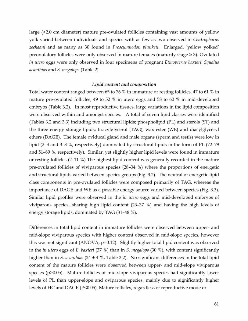
61

large (>2.0 cm diameter) mature pre-ovulated follicles containing vast amounts of yellow yolk varied between individuals and species with as few as two observed in Centrophorus zeehaani and as many as 30 found in Proscymnodon plunketi. Enlarged, ‘yellow yolked’ preovulatory follicles were only observed in mature females (maturity stage ≥ 3). Ovulated in utero eggs were only observed in four specimens of pregnant Etmopterus baxteri, Squalus acanthias and S. megalops (Table 2).

Lipid content and composition

Total water content ranged between 65 to 76 % in immature or resting follicles, 47 to 61 % in mature pre-ovulated follicles, 49 to 52 % in utero eggs and 58 to 60 % in mid-developed embryos (Table 3.2). In most reproductive tissues, large variations in the lipid composition were observed within and amongst species. A total of seven lipid classes were identified (Tables 3.2 and 3.3) including two structural lipids; phospholipid (PL) and sterols (ST) and the three energy storage lipids; triacylglycerol (TAG), wax ester (WE) and diacylglyceryl ethers (DAGE). The female oviducal gland and male organs (sperm and testis) were low in lipid (2–3 and 3–8 %, respectively) dominated by structural lipids in the form of PL (72–79 and 51–89 %, respectively). Similar, yet slightly higher lipid levels were found in immature or resting follicles (2–11 %) The highest lipid content was generally recorded in the mature pre-ovulated follicles of viviparous species (28–34 %) where the proportions of energetic and structural lipids varied between species groups (Fig. 3.2). The neutral or energetic lipid class components in pre-ovulated follicles were composed primarily of TAG, whereas the importance of DAGE and WE as a possible energy source varied between species (Fig. 3.3). Similar lipid profiles were observed in the in utero eggs and mid-developed embryos of viviparous species, sharing high lipid content (23–37 %) and having the high levels of energy storage lipids, dominated by TAG (31–48 %). Differences in total lipid content in immature follicles were observed between upper- and mid-slope viviparous species with higher content observed in mid-slope species, however this was not significant (ANOVA, p=0.12). Slightly higher total lipid content was observed in the in utero eggs of E. baxteri (37 %) than in S. megalops (30 %), with content significantly higher than in S. acanthias (24 ± 4 %, Table 3.2). No significant differences in the total lipid content of the mature follicles were observed between upper- and mid-slope viviparous species (p>0.05). Mature follicles of mid-slope viviparous species had significantly lower levels of PL than upper-slope and oviparous species, mainly due to significantly higher levels of HC and DAGE (P<0.05). Mature follicles, regardless of reproductive mode or

62

E. b

axte

ri

S. m

egal

ops

0

5

10

15

20

25

30

35

40

O V O O Ova V Ova O U V S.meg N

E.g N SP GImmature Mature In utero Mid-developed Male Male follicles follicles eggs embryos sperm testis

Tota

l lip

id (%

)█ Viv parous

▒ Oviparous

Figure 3.1 Percent total lipid content (±SD) in female and male reproductive tissues. Solid grey represent viviparous species (E. baxteri, C. crepidater, C. zeehaani, D. calcea, P. plunketi, S. megalops, and S. acanthias). Mid-developed embryos only include those from S. megalops and E. baxteri as indicated. Shaded grey represents oviparous species (C. lignaria, R. pacifica and F. boardmani). species group, had significantly higher lipid content then in any other tissue. However, in the three oviparous species (Chimaera lignaria), Rhinochimaera pacifica and Figaro boardmani), significantly lower total lipid content was observed in both immature and mature follicles than in all viviparous species (p = 0.01, Fig. 3.2). In E. baxteri, for both immature and mature follicles, maturity stage (3 to 5) was positively correlated with total lipid content (y = 1.5x + 3.1, R2 = 0.94 and y=2.1x + 26.6, R2 = 0.99). In all species, total lipid content was positively correlated with GSI (y = 3.9 GSI + 19.8, R2 = 0.60; Fig 3.4a), inferring that each are good proxies for reproductive investment. A weaker correlation was found between total lipid investment and MOD (y = 0.3 MOD + 16.6, R2 = 0.38, Fig. 3.4b). Amongst most species, PL decreased (y= –9.7 x + 63.5; R2 = 0.93) while TAG increased (y=11.4 x + 3.1; R2 = 0.96) during embryonic development (Fig. 3.5). Significantly higher PL levels were observed in immature follicles of Chimaera sp D (74 %) while significantly lower TAG levels were observed in the ova of R. pacifica (14%). The relationship between tissues and WE was inconsistent between species with similar levels in immature follicles (1–10 %), but higher levels in in utero eggs (10–12 %). Significantly higher levels of WE were found in mature follicles of oviparous G. boardmani (12–20 %). During embryonic development of S. megalops, levels of WE stayed relatively constant while PL decreased with a corresponding

63

Table 3.2 Mean percent (± SD wet weight) total lipid and lipid class composition (% of total lipid) for female reproductive tissues.

Species N MS TL(cm) ±SD Tissue detail Index HC WE DAGE TAG FFA ST PL Total Lipid %

Total Water %

Oviduct E. baxteri 1 4 84.2 - - 1.1 2.0 9.6 10.1 0.8 4.8 71.6 2.6 - S. megalops 1 4 55.8 - - 0.0 5.3 2.1 14.4 2.1 6.2 69.9 3.1 - F. boardmani # 1 4 46.1 - - 0.0 6.8 1.3 8.0 1.3 3.6 79.0 2.2 -

Immature or resting follicles No., length (cm) D. calcea 2 3–4 86 – 92 30–50, <0.9 1 20.1±1.5 4.7±0.8 7.7±1.2 16.9 ± 1.3 2.9±0.6 3.5±0.7 44.1±1.8 6.5±2.5 64.9±2.2 E. baxteri 10 3–5 64 – 84 many, <1.0 1 13.2±1.1 2.6±0.5 22.9±2.8 13.8 ± 1.5 1.4±0.5 3.2±0.9 42.9±1.4 5.7±4.1 74.7±1.3 C. crepidater 5 3–4 81 – 93 20–50, <1.1 2 16.7±3.4 3.4±0.5 6.9±2.1 18.5 ± 1.3 1.7±0.4 8.1±1.0 44.7±2.1 10.7±3.7 70.5±2.8 S. acanthias 5 4–5 59 – 81 many, <0.8 1 0.0±0.0 8.2±1.3 3.6±0.7 14.2±2.6 1.3±0.5 4.7±1.1 66.8±3.2 6.8±2.1 68.6±1.5 S. megalops 2 4–5 54 – 56 >30, <1.0 1 0.0±0.0 10.4±1.8 1.2±0.4 16.2 ± 1.4 2.3±0.7 6.0±0.8 63.9±2.1 4.1±1.8 70.4±0.9 F. boardmani # 2 4 42 – 51 2–18, 0.4-1.0 2 0.0±0.0 20.2± 1.2 3.4±0.6 10.9 ± 0.9 1.7±0.6 4.2±0.9 59.6±1.8 2.1 74.8 C. lignaria # 2 3 82–90 20–40, <0.9 1 0.0±0.9 3.4± 0.2 4.3±0.3 7.7 ± 0.5 0.4±0.1 9.9±0.6 74.3±1.3 3.3±1.9 76.1±2.4 R. pacifica # 1 4 109.6 ~40, <1.2 2 0.6 0.5 12.7 9.2 1.2 8.8 67.5 6.5 68.1

Mature pre-ovulated follicles No., MOD (cm) D. calcea 5 3–4 86 – 95 5–15, 2.2–4.3 3 30.6±3.8 2.2± 0.8 10.2±1.6 22.8± 2.3 0.3±0.2 4.4±1.0 29.4±2.5 29.8±6.2 50.6 C. zeehaani 1* 4 98.0 2, 5.4–6.1 3 23.2±2.1 0.6± 0.2 8.4±1.3 25.1± 2.0 1.5±0.7 5.4±0.7 35.8±1.4 33.8±1.9 46.8±1.7 E. baxteri 6 3–5 64 – 89 9–14, 3.6–5.2 3 19.7±4.6 3.0± 0.4 10.1±1.2 25.3±1.4 1.8±0.2 4.7±0.8 35.3±2.6 30.3±7.6 50.4±2.9 C. crepidater 5 3–4 81– 94 4–8, 2.7–5.9 3 21.1±4.6 1.9± 0.2 9.3±2.5 25.5± 3.0 1.6±0.3 4.7±1.0 35.8±2.9 34.1±3.7 50.2±2.4 P. plunketi 2 4 120 – 145 20–30, 3.4–3.6 3 3.2±0.8 0.8± 0.2 27.8±2.7 18.6± 2.1 1.5±0.5 3.7±0.3 44.3±1.7 28.2±2.2 48.2 S. acanthias 3 4–5 67 – 81 8, 2.2–4.1 3 0.1±0.0 1.0± 0.5 11.6±0.9 33.6± 1.6 2.0±0.6 1.0±0.4 48.7±1.9 30.3±3.8 51.8 S. megalops 2 4 54.3–55.8 3, 3–3.4 3 0.1± 0.0 9.7± 1.3 7.2±1.1 26.8± 1.7 1.6±0.5 6.9±1.1 47.6±2.3 29.1±2.1 53.2±1.5 F. boardmani # 2 4 42 – 51 4–7, 1.7–2.1 3 0.0± 0.0 12.1± 1.3 6.0±1.5 26.2± 2.9 1.9±0.9 5.6±1.0 48.2±3.7 18.1±1.7 61.1 C. lignaria # 2 3–4 90 – 111 4, 2.1–3.4 3 0.0± 0.2 5.6± 0.8 12.4±0.8 27.1± 1.1 1.1±0.3 5.8±0.5 47.9±1.5 19.4±3.5 54.3 R. pacifica # 1 4 109.6 9, 3.3–4.6 3 0.3 5.0 22.1 14.3 0.7 4.4 53.1 24.1 -

In utero eggs Weight (g) E. baxteri 1 5 84.2 221.3 5 3.4 9.6 4.2 40.7 1.6 5.0 35.5 36.9 50.9 S. acanthias 2 5 78 – 81 87–112.2 3-4 0.2±0.1 11.5±1.3 4.7±1.2 36.4±3.1 1.3±0.2 5.7±0.4 40.1±2.8 24.0±3.6 52.1±4.0 S. megalops 1 5 55.8 37.8 5 0.0 11.0 8.9 41.3 1.1 7.7 30.0 30.3 49.2 Mid-developed embryos No., length (cm) E. baxteri 2 - 84.2 4-7, 7.3–10.3 0.9±0.3 4.2±0.8 10.8±1.9 48.3±2.2 2.3±0.8 4.3±0.7 29.2±2.0 25.1±2.5 60.1 S. megalops 1 - 55.8 2–3, 12.8–14.6 0.0 7.6 0.2 30.9 1.8 5.1 54.3 22.6 58.6

N – number of individuals; MS – Maturity stage (after Daley et al. 2002b); TL – Total length of female; Index: Assignment of ovary and uterus condition based on Walker (2005); HC – Hydrocarbon, WE – Wax esters, DAGE - diacylglyceryl ethers, TAG – triacylglycerols, FFA – free fatty acids, ST – Sterols, PL – Polar lipid. # represents species that undertake oviparous reproduction. * For C. zeehaani, replicate analyses are for different eggs of the same individual. For percentage total water content, representative samples were chosen with n = ≤ 2. Embryos of S. megalops ranged between 12.8 to 14 cm TL and for E. baxteri between 7.3 and 10.3 cm TL.

64

0

10

20

30

40

50

60

C. zeehaani Upper-slopesqualids

Mid-slopesqualids

Chimaeras G. boardmani

Lipi

d (%

)Total lipid Energetic lipidsStructural lipids

Figure 3.2 Proportion of percent (%) total lipid content and proportion of total energetic lipids (TAG, WE and DAGE) and structural lipids (PL and ST) in preovulatory follicles (≥ stage 3) for major taxon groupings.

Figure 3.3 Histogram showing proportion of the three energy lipid classes in mature preovulatory follicles of the major taxon groups. WE, wax ester; DAGE, diacylglycerol; TAG, triacylglycerol.

0.0

0.2

0.4

0.6

0.8

1.0

C. zeehaani Upper-slopesqualids

Mid-slopesqualids

Chimaeras G. boardmani

Prop

ortio

n

WEDAGETAG

65

increase in TAG (Fig. 3.6a). Total lipid content increased rapidly during the development of enlarged ova and then decreased when eggs became fertilized and in developing embryos. In E. baxteri, total lipid and TAG continued to increase throughout tissue development until eggs became fertilized with subsequently less lipid and TAG in mid-developed embryos (Fig. 3.6b). WE remained constant between immature and mature follicle development, then increased after fertilization with moderate amounts found in mid-developed embryos. Similar to S. megalops, PL decreased in mature follicles until fertilized and increased in mid-developed embryos. Taxon differences in the lipid class composition of the female reproductive tissues were clearly represented by multidimensional scaling analyses (MDS, Fig. 3.7). In mature males, testis and sperm lipid content varied among tissue, with slightly higher lipid content found in sperm (sperm 3–8 %, testis 3–4 %)(Table 3.3). Similar lipid class profiles were observed in both tissues with PL (51–89%) dominating; however, they were grouped separately by MDS cluster analyses. In all male and female reproductive tissues the PL fraction consisted of predominately PC (phosphatidylcholines, 85-97%), followed by PE (phosphatidylethano-lamine, 3-13%) and traces of PS (phosphatidyl serine) and CL (cardiolipin, <2%). Variable levels of HC and DAGE were observed in all female and male reproductive tissues of some species which also had HC and DAGE in the liver (Pethybridge et al., 2010). FFA in all tissues ranged between 1.5 and 2.9 %, indicating good sample integrity with low lipolytic and enzyme activity since collection (Jeckel et al., 1989).

Fatty acid profiles

The fatty acid composition of different female reproductive tissues was similar amongst all species with most tissues high in MUFA and dominant fatty acids including 18:1ω9, 16:0, 22:6ω3, 20:1ω9, 22:1ω11 and 22:6ω3 PUFA (Table 3.4). MUFA levels increased between immature and mature pre-ovulated follicles while SAT and PUFA levels increased after ovulation and storage of uterine yolk (Figure 3.8a). Ratios of ω3/ω6 correlated with increasing stage of embryonic development (y= 1.0x + 0.9, R2=0.90). This was mainly due to increasing levels of DHA (22:6ω3) and corresponding decreasing levels of AA (20:4ω6), particularly between immature and mature follicle development (Figure 3.8b). Higher levels of DHA were observed in uterine yolk (22± 5 %) than in mature follicles (12 ± 4 %) and was more than double of that found in immature follicles (9 ± 3 %).

66

In contrast significantly higher levels of AA were found in the immature follicles (11 ± 5 %) than in all other tissues (3 ± 1 %). Levels of 18:1ω9 and 20:1ω9 were much higher in the mature follicles than in other tissues while levels of 18:0 were lower.

y = 3.9x + 19.8R2 = 0.60

10

20

30

40

50

0 1 2 3 4 5 6

GSI (% whole body)

Lipi

d (%

)

y = 0.3x + 16.4R2 = 0.38

10

20

30

40

50

10 20 30 40 50 60 70

MOD (mm)

Lipi

d (%

)

Figure 3.4 Relationship between maternal total lipid for pre-ovulatory mature follicles (stage 3, Daley et al. 2002b) and a) female gonadosomatic index, GSI; and b) mean ovarian diameter, MOD, in all species represented by the symbols: ○ E. baxteri, ∆C. crepidater, □ P. plunketi, ◊ D. calcea, + C. zeehaani, ●S. acanthias, ♦S. megalops, ■Chimaera spp (C. lignaria and R. pacifica), ▲F. boardmani

B.

A.

67

WE

∆TAG

y = -9.7x + 63.5R2 = 0.93

y = 11.4x + 3.1R2 = 0.96

0

10

20

30

40

50

60

70

80

0.5 1.5 2.5Immature Mature In utero follicles follicles egg

lipid

(%) ○ PL

Figure 3.5 Composition of major lipid classes (phospholipid, PL; triacylglycerols, TAG; and wax esters,WE) for demersal shark species during 3 stages of embryonic development. Solid symbols represent outliers including (■) WE outliers representing F. boardmani; (▲) TAG outlier – R. pacifica and (●) PL outlier – C. lignaria. No mid-developed embryos of oviparous species were assessed.

Higher levels of 20:1ω9 and 22:1ω11 were observed in viviparous follicles than in oviparous egg-case yolk, however these differences were not significant. The FA profile of the egg case yolk from the oviparous catshark, G. boardmani differed from all other species, including oviparous C. lignaria, with significantly higher levels of 16:0 and DHA, and lower levels of 18:1ω9 and 20:1ω9. In female reproductive tissues, fatty alcohol and glyceryl ether diols (Alc/GED derived from DAGE) were also present and were highest in mature pre-ovulated follicles (10.0 to 17.2 % relative level compared to total FA) and lowest in the mid-developed embryo of S. megalops (0.7%). Dominant Alc/GED in most mature and immature follicles was 18:1ω9GED, 16:0GED, 22:1ω9.

In mature males, similar FA profiles were observed in the sperm and testis with high

levels of PUFA (34– 47%) and moderate amounts of SAT (23 – 33 %) and MUFA (20 – 33

%) (Table 3.3). Major FA included: 18:0, 22:6ω3, 18:1ω9, 16:0 and 22:4ω6 in descending

68

Figure 3.6 Total lipid content (% wet weight) and relative contributions (% of total lipids) of structural phospholipids (PL), and energetic lipids, triglyceride (TAG), diacylglyceryl ethers (DAGE) and wax esters (WE) for A) S. megalops (n=1-2) and B) E. baxteri (n=1-3) during 4 stages of embryonic development.

B.

A.

69

Table 3.3 Mean (± SD) percentages of total lipid content, lipid class and FA composition (% wet weight) of male reproductive tissues. All males were fully mature (Stage 5; Walker 2005).

Aplacental Viviparous Oviparous Sample C. zeehaani C. crepidater D. licha S. megalops C. lignaria

tissue Sperm Testis Sperm Testis Sperm Testis Sperm Testis Sperm Testis No 1 1 3 3 1 1 1 1 1 1 TL (cm) 87.0 78.4 – 82.3 111.9 41.5 75.3 Total lipid % 5.4 3.3 4.5 ± 1.0 2.7 ± 0.8 3.7 3.1 7.9 2.5 6.0 4.1 Lipid Classes HC (SQ) 6.4 6.1 5.4 ± 0.9 7.3 ± 1.8 8.3 0.7 0.0 0.0 1.0 0.0 WE 8.4 12.0 3.4 ± 0.7 2.1 ± 0.3 10.1 1.0 2.0 2.8 0.0 0.0 DAGE 17.3 11.4 5.3 ± 0.5 1.4 ± 0.3 2.9 4.2 0.5 0.0 0.7 2.3 TAG 7.0 5.0 6.2 ± 1.0 4.8 ± 0.7 14.0 27.2 4.0 5.5 6.0 9.2 FFA 1.3 2.0 1.6 ± 0.3 3.3 ± 1.0 0.6 1.2 3.6 0.5 1.4 1.9 ST 9.9 4.9 5.7 ± 0.5 5.2 ± 1.0 5.3 2.7 4.7 3.0 3.7 3.0 PL 51.0 58.6 72.4 ± 3.9 75.9 ± 4.7 58.9 63.2 86.3 88.7 87.3 83.6

Fatty Acids 14:0 0.9 0.7 0.5 ± 0.1 0.4 ± 0.0 0.0 0.2 0.0 0.2 0.0 0.4 16:0 9.8 9.0 11.6 ± 1.0 17.1 ± 1.4 8.4 13.2 9.1 12.4 9.4 12.3 17:0 2.0 1.8 0.9 ± 0.1 1.5 ± 0.7 0.9 1.4 0.9 1.2 1.2 0.6 18:0 19.2 11.9 17.5 ± 2.1 6.5 ± 3.5 18.5 10.7 18.4 13.3 17.4 15.0 ∑SAT 32.7 23.6 32.8 ± 1.6 25.0 ± 2.1 28.9 26.3 28.6 27.4 28.3 27.3 16:1ω9 0.0 0.0 0.2 ± 0.1 0.3 ± 0.2 0.0 0.8 0.0 0.0 0.5 0.0 16:1ω7 1.0 2.9 0.3 ± 0.2 1.1 ± 0.4 0.3 0.8 0.4 1.0 0.8 1.2 18:1ω9 12.9 11.6 7.0 ± 1.1 10.7 ± 1.1 8.6 13.3 14.9 13.8 17.3 15.6 18:1ω7 0.5 0.5 4.4 ± 0.8 5.1 ± 0.3 4.0 3.6 5.5 4.8 5.5 2.3 18:1ω5 0.9 0.7 0.4 ± 0.1 0.4 ± 0.2 0.5 0.2 0.3 0.3 0.4 0.6 20:1ω9 2.3 4.6 5.4 ± 0.9 7.5 ± 1.2 6.0 8.1 5.3 6.2 6.7 5.9 20:1ω7 * 0.8 0.4 0.6 ± 0.1 0.3 ± 0.2 0.6 0.4 0.3 0.0 0.4 0.4 22:1ω11 1.1 1.7 0.5 ± 0.2 0.5 ± 0.3 1.1 2.5 0.1 0.5 0.3 0.8 22:1ω9/ω7 0.3 0.2 0.6 ± 0.2 1.0 ± 0.3 1.1 1.3 0.2 0.6 0.3 0.0 24:1ω11/ω9 * 0.5 1.1 0.1 ± 0.0 0.8 ± 0.3 0.0 0.3 0.4 1.3 0.0 0.4 ∑MUFA 20.6 24.5 19.7 ± 1.4 28.4 ± 1.2 23.0 32.3 28.0 29.0 33.4 27.1 18:2ω6 2.3 2.5 1.3 ± 0.5 0.9 ± 0.7 1.7 1.1 1.1 0.9 0.8 0.5 20:2ω6 1.9 0.7 0.7 ± 0.2 0.4 ± 0.2 0.9 0.3 0.2 0.2 0.3 0.5 20:4ω6 (AA) 9.7 9.5 12.8 ± 2.6 10.0 ± 3.1 13.0 9.5 10.7 11.3 10.5 9.2 22:4ω6 0.0 15.5 3.9 ± 0.4 3.4 ± 0.5 7.3 4.3 1.3 2.7 1.3 4.4 22:5ω6 0.0 0.0 0.7 ± 0.2 0.6 ± 0.2 1.4 0.7 0.8 0.8 0.6 0.2 20:4ω3 2.0 0.7 0.2 ± 0.1 0.7 ± 0.1 0.4 0.7 1.5 1.6 0.4 0.9 20:5ω3 (EPA) 1.4 1.1 0.3 ± 0.2 2.9 ± 2.0 0.5 1.2 3.2 4.3 2.4 3.8 22:5ω3 (DPA) 4.6 4.3 7.6 ± 0.8 7.0 ± 1.3 5.6 5.6 3.9 5.0 3.7 4.2 22:6ω3 (DHA) 14.4 6.2 15.7 ± 1.1 14.7 ± 0.9 12.3 10.3 18.5 13.4 13.0 15.1 ∑PUFA 39.1 47.4 44.7 ± 1.6 41.8 ± 0.9 45.9 34.7 42.4 42.0 33.6 38.7 Bramched/iso 2.9 2.1 1.9 ± 0.4 2.2 ± 0.9 1.3 3.3 0.8 1.1 2.0 1.4 phytanic acid 0.8 0.8 0.9 ± 0.3 0.8 ± 0.5 1.7 1.3 0.5 0.9 1.2 1.0 Others ** 5.3 4.0 2.0 ± 0.8 3.7 ± 1.1 3.9 2.7 1.4 2.1 3.6 2.4 ω3/ω6 1.7 0.5 1.3 1.7 0.9 1.2 2.0 1.6 1.5 1.6

Footnote for lipid composition as per Table 3.2. For Fatty Acids: % Alc/GED (Percent fatty Alcohol/ glyceryl ether diols) values are taken before separation from total FA. Dominant Alc/GED in ova include: 18:1ω9GED, 16:0GED, 22:1ω9. AA, arachidonic acid; EPA, eicosapentaenoic acid; DPA, docosapentaenoic acid; DHA, docosahexaenoic acid; SAT, saturated faty acids; MUFA, monounsaturated fatty acids; PUFA, polyunsaturated fatty acids. *20:1 ω7 may contain 20:3ω3, 24:1ω9 celutes with 18:0GED, and 22:4ω3 may include 22:2NMI. Branched FA include: i15:0, i16:0, i17:0, i18:0, br17:1 and 7Me17:1. **other FA include those <0.2%: 20:0, 22:0, 24:0, 17:1ω6, 18:1ω7t, 19:1, 20:1, 21:5ω3, 18:3ω6, 20:3ω6, 21:5ω3, 22:3ω6

70

Table 3.4 Percentage fatty acids (mean % wet weight ± SD) for reproductive tissues of deepwater chondrichthyan species

Reproductive mode Aplacental Viviparous Oviparous Habitat Mid-slope Upper-slope Mid-slope Upper-slope Species E. baxteri C. crepidater D. calcea P. plunketi S. acanthias S. megalops C. lignaria F. boardmani

tissue Immature

follicles Mature follicles

Uterine yolk

Immature follicles

Mature follicles

Immature follicles

Mature follicles

Mature follicles

Immature follicles

Uterine yolk

Immature follicles

Uterine yolk

Mid-dev embryo

Egg case yolk

Immaturefollicles

Egg case yolk

No. 4 5 1 1 5 1 5 2 5 2 1 1 1 1 2 2 maturity 4-5 3-4 1 4 3-5 2 4-5 2 4-5 3-5 3 5 - 3 3-4 3-5 14:0 0.6±0.1 1.0±0.3 1.1 0.7 1.2±0.5 0.9 0.8±0.3 0.8±0.7 0.9±0.3 0.9±0.5 0.6 1.4 0.6 0.2 1.2±0.4 1.2±0.3 15:0 0.3±0.0 0.4±0.2 0.6 0.3 0.2±0.1 0.4 0.3±0.1 0.3±0.1 0.4±0.2 0.3±0.1 0.3 0.5 0.4 0.0 0.5±0.1 0.5±0.2 16:0 15.3±2.0 11.3±2.5 14.1 16.8 16.3±3.2 13.7 16.8±2.9 12.3±2.0 15.9±1.8 15.0±3.3 12.8 16.7 19.2 10.9 17.6±2.3 18.4±2.7 17:0 0.7±0.1 0.5±0.2 0.4 0.9 0.5±0.2 0.7 0.4±0.1 0.6±0.1 0.7±0.1 0.8±0.1 2.2 0.8 1.0 0.8 1.0±0.3 0.7±0.1 18:0 0.8±0.1 0.7±0.6 2.5 6.7 1.7±0.9 4.4 2.2±1.2 2.5±1.2 6.0±1.4 6.0±1.7 2.5 4.1 4.9 0.7 6.9±1.2 5.0±0.5 ∑SAT 18.5±1.5 14.4±2.4 19.2 25.3 20.6±3.9 21.0 20.1±3.5 17.2±2.6 24.1±3.3 23.3±3.0 19.8 23.9 26.3 13.6 27.9±3.2 26.7±4.6 16:1ω9 0.5±0.2 0.6±0.2 0.6 1.2 0.3±0.4 0.2 0.1±0.1 0.4±0.2 0.3±0.3 0.3±0.1 0.7 0.2 0.4 1.2 0.2±0.2 0.3±0.1 16:1ω7 2.3±0.1 3.0±1.1 3.3 2.4 3.4±0.7 1.9 2.5±1.1 2.0±0.2 1.8±0.4 2.1±1.2 1.7 2.6 2.3 3.2 3.0±0.8 4.0±0.9 18:1ω9 19.8±1.0 23.6±4.3 17.3 12.7 23.3±1.9 12.6 22.7±3.5 20.3±3.1 14.0±1.5 16.6±1.9 18.2 14.4 18.5 27.5 15.9±3.4 18.8±1.5 18:1ω7 4.0±0.1 4.0±0.2 5.0 9.1 3.8±0.8 5.1 3.6±1.3 3.7±1.2 5.6±1.3 5.4±0.2 6.7 5.0 7.6 8.2 5.6±0.3 3.3±0.8 18:1ω5 0.4±0.1 0.3±0.1 0.4 0.8 0.3±0.2 0.4 0.3±0.1 0.4±0.1 0.4±0.2 0.5±0.3 0.4 0.2 0.0 0.6 0.6±0.2 0.3±0.0 20:1ω9 12.2±3.3 16.6±4.1 8.5 1.7 9.1±1.5 12.6 8.5±1.9 15.1±1.6 8.7±2.4 8.8±4.0 4.7 8.2 6.4 7.6 11.3±1.7 5.9±1.7 20:1ω7c 0.7±0.1 0.7±0.2 0.6 0.5 0.6±0.2 0.6 0.4±0.3 0.8±0.1 0.7±0.5 0.5±0.3 1.8 0.3 0.4 1.4 0.8±0.1 0.4±0.1 22:1ω11 7.0±2.2 9.3±2.2 3.6 0.0 4.1±1.1 6.9 3.5±1.1 9.1±1.8 1.2±0.6 3.1±1.2 0.0 2.9 1.4 4.6 0.8±0.4 2.2±1.0 22:1ω9/7 3.4±0.8 3.2±0.9 2.2 1.2 3.0±1.2 1.7 3.6±1.6 2.8±1.1 2.0±1.1 2.2±0.5 2.4 0.1 0.6 3.5 1.6±0.9 1.1±0.5 24:1ω11/9 0.9±0.1 1.0±0.2 0.9 0.5 2.3±0.7 1.1 2.7±0.2 0.8±0.3 1.1±0.3 1.1±0.2 0.2 0.2 0.0 0.6 0.2±0.0 0.2±0.2 ∑MUFA 51.9±6.7 62.9±3.1 42.5 30.5 50.6±4.5 43.5 48.5±7.0 55.6±4.1 36.9±4.2 40.8± 5.3 36.8 34.1 38.2 58.2 44.3±5.5 37.3±6.0 18:2ω6 0.9±0.1 0.6±0.4 1.0 1.5 0.8±0.5 0.5 1.1±0.4 0.6±0.2 0.8±0.3 1.6±1.0 1.2 1.4 0.5 0.8 0.8±0.3 1.1±0.5 20:2ω6 0.4±0.1 0.4±0.1 0.3 0.2 0.1±0.2 0.3 0.1±0.1 0.3±0.1 0.4±0.1 0.4±0.3 1.0 0.4 0.4 0.6 0.4±0.1 0.3±0.0 20:4ω6 (AA) 6.2±2.4 3.8±2.0 4.9 18.5 2.8±0.9 7.1 3.6±1.4 3.7±1.6 10.6±2.4 4.6±2.6 14.6 2.6 2.5 4.0 7.5±2.1 2.6±0.6 22:4ω6 0.9±0.2 0.6±0.5 1.0 0.5 0.5±0.4 0.8 0.8±0.4 0.7±0.2 0.6±0.2 1.1±0.5 1.1 1.1 1.3 0.8 0.7±0.3 0.7±0.5 22:5ω6 0.4±0.1 0.3±0.2 0.4 0.0 2.0±1.7 0.9 0.6±0.3 0.5±0.2 0.4±0.2 0.9±0.3 0.0 0.0 0.9 0.0 0.8±0.1 0.5±0.4 20:4ω3 0.6±0.1 0.3±0.2 0.9 0.3 0.8±0.4 1.8 0.6±0.4 1.0±0.5 0.9±0.4 1.4±0.2 0.7 1.1 0.5 0.3 0.8±0.3 0.9±0.3 20:5ω3 (EPA) 3.4±1.4 2.2±1.2 1.3 1.4 4.6±1.3 3.4 4.6±1.6 3.2±1.2 5.2±0.9 4.3±0.7 1.3 3.0 2.1 0.3 1.3±0.4 5.1±0.6 22:5ω3 (DPA) 2.0±0.2 1.7±0.9 3.6 1.5 1.6±0.4 3.2 1.9±0.8 2.0±0.9 1.7±0.6 4.1±0.9 3.6 3.7 3.5 2.7 1.9±0.5 2.2±1.1 22:6ω3(DHA) 8.9±1.4 6.9±2.2 18.6 11.3 9.4±3.7 10.9 12.9±4.1 10.1±3.5 8.5±2.2 13.8±1.9 4.5 25.1 19.2 10.2 12.0±2.5 18.0±4.0 ∑PUFA 23.6±5.2 18.8±4.5 31.1 38.4 23.7±5.5 30.9 27.7±6.3 23.6±4.6 29.1±5.5 34.0±4.7 30.2 39.2 31.6 22.8 27.0±3.0 32.4±5.3 Branched/iso 2.2±0.2 1.7±0.4 2.9 2.4 1.7±0.5 1.0 1.5±0.2 1.6±0.2 1.6±1.2 1.4±0.3 5.6 1.3 1.1 2.4 2.3±0.8 1.6±0.2 phytanic acid 1.2±0.1 1.3±1.0 1.6 0.6 0.6±0.6 0.9 1.2±0.4 0.6±0.2 0.8±0.3 0.9±0.5 1.6 0.2 1.0 1.0 1.3±0.4 0.6±0.4 others ** 4.0±0.8 2.8±1.1 2.6 2.9 4.3±2.7 4.0 2.7±0.5 3.4±0.4 2.3±1.8 2.6±0.6 3.8 2.2 2.8 5.0 1.1±0.5 3.5±1.3 ω3/ω6 2.2 2.0 3.3 0.7 2.7 2.1 3.3 2.9 2.4 2.7 0.6 5.9 4.5 2.2 2.2 5.0

% Alc/GED 15.4±2.9 17.2±6.7 10.3 4.4 12.3±4.2 5.3 10.0±2.8 13.8±4.2 4.9±2.2 4.9±2.5 8.7 3.8 0.7 17.4 6.2±1.1 3.2±0.5

Footnote as per Table 3.3.

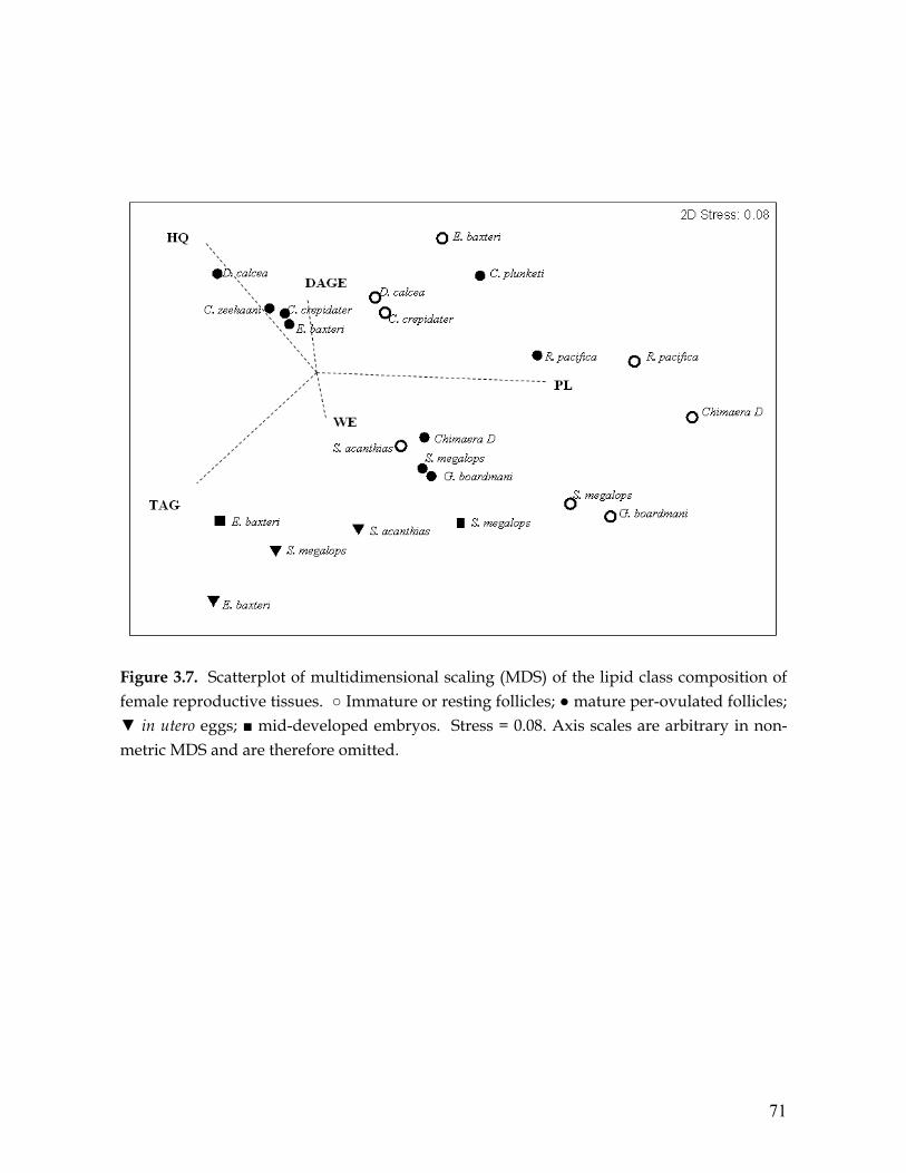
71

Figure 3.7. Scatterplot of multidimensional scaling (MDS) of the lipid class composition of female reproductive tissues. ○ Immature or resting follicles; ● mature per-ovulated follicles; ▼ in utero eggs; ■ mid-developed embryos. Stress = 0.08. Axis scales are arbitrary in non-metric MDS and are therefore omitted.

72

0

10

20

30

40

50

60

0 1 2Immature Mature follicles follicles

FA (%

)

ω3/ω6

∑SAT

∑MUFA

∑PUFA

3 4 In utero Mid-developed eggs embryos

0

5

10

15

20

25

30

0 1 2Immature Mature follicles follicles

FA (%

)

18:1ω9

20:4ω6 (AA)

22:6ω3 (DHA)

3 4 In utero Mid-developed eggs embryos

Figure 3.8 A) Major FA groups, monounsaturated (MUFA), poly unsaturated (PUFA), and saturated (SAT) and B) major individual FA in female reproductive tissues for demersal chondrichthyan species. AA, arachidonic acid; DHA, docosahexaenoic acid.

< Pre-ovulation Post-ovulation >

< Pre-ovulation Post-ovulation > B.

A.

73

order of importance. Despite similarities in FA profiles, MDS analyses grouped both

tissues separately due to higher levels of 22:4ω6 and 16:0 being observed in the testis while

higher levels of 18:0 and 20:4ω6 were found in sperm (unpublished data). Significantly

higher levels of 18:0 were found in both male reproductive tissues than in all female tissues

(t-test, p = 0.02). Similar ω3/ω6 PUFA ratios and levels of AA were found in the ovarian

follicles of females and both male reproductive tissues (11 ± 5% and 11 ± 1 %, respectively).

3.4 DISCUSSION General reproductive biology

All sharks analysed in the present study were of adult size (Daley et al. 2002b) and all

maximum ova diameters, litter size and embryo sizes fell within those that have been

recorded for these species in larger data sets (eg. Watson & Smale 1998; Irvine 2004; Daley

et al. 2002b). The water content of female reproductive tissues was similar between all

species with higher water content found in lipid poor tissues. Slightly higher relative water

content was observed in oviparous species which corresponded to lower lipid content.

Water content in the oviduct (72–78 %) is similar to that reported in the muscle (Økland et

al. 2005). In ovarian follicles, moderately high water content was observed in squalid

dogfish (47–54 %), within the range reported by Remme et al. (2005). Many of these

chondrichthyan species have a resting stage within and between pregnancies and that is

why pre-ovulated eggs are rare.

Lipid content and composition of reproductive organs

Of my current knowledge, this is the first study to investigate the role of lipid in relation to

embryonic development in deepwater chondrichthyans. All male and female reproductive

tissues had high lipid content in comparison to the muscle, kidney and pancreas but are

significantly lower than that reported in the liver (Chapter 2). As expected, distinct gender

differences in the reproductive role of lipids and their usages were found between males

and females. In mature males, the lipid content was slightly higher in sperm (3–8 %) than

in testis (3–4 %) possibly corresponding with higher levels of investment so as to increase

male fertility. In females, lowest lipid levels were found in tissues that play a more

74

organizational role (oviduct, 2–3 % ww) or that are undeveloped (immature follicles, 2–

11%). The highest lipid reserves were observed in more developed reproductive tissues

(mature follicles, 22–39 %; in utero eggs, 24–37 %; and mid-developed embryos, 22–26 %),

and indicate high levels of maternal investment. In addition, the marked increase of lipid

content in ovarian follicles with maturation alludes to the importance of lipid in embryonic

development of deepwater chondrichthyans. Comparable amounts of lipid have been

found in the mature follicles of Centrophorus and Centroscymnus species (Shimma & Shima

1968; Remme et al. 2005). Andre and Canal (1929) reported the lipid content of an ovarian

follicle of Centrophorus at mid-development was 29.6 % wet weight (ww), similar to those in

this study. Remme et al. (2005) recorded protein and amino acid (ash) percentages in

ovarian follicles between 20 to 26 % and 2 to 4 % ww, respectively, and here we can assume

that similar levels are observed in these species. In utero eggs in the first stage of

development (according to Walker 2005) and mid-developed embryos had similar levels to

those reported in Centrophorus granulosus by Guallart and Vicent (2001). Noble and Cocchi

(1990) found that during the second stage of embryonic development (after ovulation) that

there is an increase in lipid utilization and transfer from the yolk, which despite the small

sample size used in this study, seems plausible in these deepwater species. In E. baxteri,

the total lipid content of immature or resting follicles and mature pre-ovulated follicles

within the ovary were correlated with maturity stages. Similar correlations have been

shown in fish (Wiegand 1996) and squid (Clark et al. 1994) and indicate increasing levels of

maternal investment during the gestation period. Due to small sample sizes it was not

possible to obtain such information for other species. However, total lipid content was also

correlated with female GSI regardless for all species combined and emphasis that those

species that produce larger ovarian eggs relative to body weight, invest more in

reproduction.

Wourms et al. (1988) suggested that the dependency of developing embryos on maternal

nourishment is widespread across sharks species, describing that an almost continuous

gradient exists from none to almost complete nourishment. There are a number of studies

that suggest that there is around a 50% loss of organic matter during embryonic

development (Ranzi 1932; Wourms 1981, Wourmes et al. 1988). This study shows similar

75

findings with total lipid content in mid-developed embryos lower than in utero eggs for

both S. megalops and E. baxteri. Therefore, similar to conclusions by Guallart and Vicent

(2001) for C. granulosus, and Braccini et al. (2007) for S. megalops, these findings suggest that

in E. baxteri, S. acanthias and S. megalops there is little or no maternal contribution of organic

matter after ovulation and during embryonic development in the uterus.

Differential provisioning of lipid and other nutrients during embryonic development has

important consequences for offspring fitness. The shift between the dominance of PL to

that of TAG over the reproductive cycle of female sharks, as shown in this study,

demonstrates the initial establishment of structural lipids (PL and ST) followed by an

increase investment in storage lipids (TAG, WE and potentially DAGE) which peaks at the

time of fertilization (Fig. 3.5–3.6). The well established role of PL and ST in marine

organisms is for the preservation of the structure and function of cellular membranes

(Sargent et al. 2002). In chondrichthyans, follicles contained dominant levels of structural

lipids and illustrate the relative importance of these lipids throughout embryonic

development and particularly in the early stages of maturation. In contrast ST remained

constant throughout maturation suggesting that its function has little influence on

embryonic development. Sterol in higher animals and invertebrates has been shown to be a

precursor to hormones, bile salts and vitamin D (Kanazawa 2001).

As found here, for deepwater chondrichthyans, TAG is the major energy lipid used to

support embryonic development. Maternal TAG provisions are widely recognized in

numerous animals as a necessary component for reproduction and maturation as it is the

primary mode of lipid transport and the preferred form for storage (Sargent 1995). TAG

levels found in the pre-ovulated eggs of chondrichthyes reported in this study were within

the higher range bracket of those found in certain marine fish that have long incubation

times (Wiegand 1996; Mourente et al. 1999) while higher levels are reported in birds and

reptiles (Noble 1991). In this study, female chondrichthyans had moderate to high levels of

TAG in all tissues with highest levels found in mature ovarian follicles (23 ± 5 %) and in

utero eggs (39 ± 3 %). Lower levels of TAG ( 4 – 19 %) are found in the livers of mid-slope

Squaliformes and Chimaeras while much higher levels (44 – 80 %) are found in the liver of

76

shelf and upper-slope species including the catshark F. boardmani (Chapter 2). This could

explain the slightly higher levels of TAG observed in both the oviduct and mature follicles

of S. acanthias, S. megalops and F. boardmani, which also represent the three fastest growing

species examined in this study.

Remme et al. (2005) reported much higher levels of TAG in the developed follicles of 4

species of mid-slope squaliformes (35–55 % total lipids) than were reported here for all

squaliforme species (18–34 %). However, in the study by Remme et al. (2005) lipid fractions

of both HC and DAGE were not reported which in this study accounted for large

percentages of the total lipid fraction (33 ± 9 %). Thus, if we excluded these two lipid

classes, similar TAG fractions may have been recorded. Similar TAG levels were observed

in the mature pre-ovulated follicles of all elasmobranchs, regardless of reproductive mode,

suggesting similar usages of TAG in their reproduction. In comparison, the two

holocephalans, R. pacifica and C. lignaria had lower TAG levels and much higher DAGE

levels than other species. The TAG-rich lipids of chondrichthyan eggs represent a resource

of concentrated energy, ideally suited to sustaining embryonic development throughout the

long gestation period. In male organs, high levels of TAG were found in the testis and

sperm of Dalatias licha (27 and 14 %, respectively) whilst in other species levels were more

similar to the female oviduct (5 – 10 %). These high amounts of TAG in D. licha were not

correlated to increased WE or total lipid content and could suggest a greater need for this

storage lipid which in its cellular context is relatively inert until required.

Wax esters (WE) occurred in all reproductive tissues and at much higher concentrations

than in the liver, kidney, muscle and pancreas (Chapter 2). In both male and female

reproductive tissues, WE generally was the second most important storage lipid with

significantly higher levels of TAG than WE, with the exception of immature follicles of the

oviparous F. boardmani which had higher WE levels (20 ± 1 %) than TAG (11 ± 1 %), and

mature C. zeehaani males where WE (8–12 %) were higher than TAG (5–7 %). F. boardmani

had the highest WE concentrations in all female tissues than in all other species suggesting

that it employs a different reproductive strategy or that the utilization and possible function

of WE is different in this species. WE is normally deemed a long-term storage of energy,

77

used when food resources are low (Nicol et al. 2004). WE has been found in large

proportions in scombroid fish (Kaitaranta and Ackman 1981) and it has been suggested that

WE formation may be a biochemical mechanism for elaborating lipids at unusually high

rates from amino acid and glucose precursors (Nevenzel 1970). In viviparous species

examined in this study, WE levels, similar to total lipid content and TAG levels, peak at the

time of fertilization where eggs are ovulated before being transferred to the uterus.

Similarly to other marine animals, a number of possible functions of WE in chondrichthyan

reproduction include; long–term energy reserve; buoyancy, permeability control, and fatty

acid reserve for modifying structural lipids after egg fertilization (Nevenzel 1970; Lee and

Patton 1989; Sargent et al. 2002).

The presence of DAGE and hydrocarbon (HC) in male and female reproductive tissues has

not, to my knowledge, been previously recorded in any chondrichthyan species analysed to

date. Significant correlations were made between species which have DAGE and HC in

reproductive tissues and those that have high quantities in the liver (Chapter 2). HC,

mainly in the form of squalene, has been recorded in a number of deepwater sharks, mainly

in Squaliformes occupying depths greater than 600 meters (Nevenzel 1989; Deprez et al.

1990; Hernández-Perez et al. 1997). HC is metabolically inert and thus is believed to have

buoyancy as its only function (Nevenzel 1989). DAGE is the major lipid present (>50%) in

the livers of certain deep sea sharks (Deprez et al. 1990; Bakes & Nichols 1995), and

holocephalans (Hayashi & Takagi 1982; Sargent 1989). It is also present in teleost fish

(Hayashi et al. 1978), deep-sea squids (Hayashi et al. 1990; Hayashi & Kishimura 2002) and

in the ovaries of starfish (Hayashi 1997). The presence of DAGE in the reproductive tissues

of sharks and Chimaeras is intriguing as the biological role in marine organisms is not well

known. Numerous functions of DAGE have been postulated including; buoyancy

regulation (Sargent et al. 2002; Phleger 1998), secondary energy source (Sargent 1989) or it

may aid in many cellular processes, modulating vital biochemical mechanisms (Sargent et

al. 2002). In squid, Hayashi and Kishimura (2002) suggested that DAGE acts as metabolic

energy reserves fuelling development in the absence of externally available food, similarly

to WE in deep-sea fish. Böer et al. (2005) found high DAGE levels in zooplankton, and also

assumed that DAGE is necessary during periods of food scarcity, and that it may also serve

78

as an additional energy source during reproduction. It is not considered likely that DAGE

and HC are directly obtained through the diet. A possible alternative source of DAGE is

the conversion of dietary derived WE to glyceryl ethers via an unspecified metabolic

pathway in the liver of sharks, as found by Malins and Sargent (1971) in S. acanthias. Large

and variable levels of DAGE (0.2–28 %) in the reproductive tissues of all chondrichthyan

species, suggest that it may be an important lipid class used as an additional energy source

in developing embryos. Wiegand et al. (2004) showed that some fish use yolk-lipids

(especially neutral lipids) as nutrient and caloric reserves both during and following

embryogenesis. Similarly to findings of Wiegand (1996), shark egg lipids seem to be

derived from dietary lipids, where lipids are mobilized from body reserves, synthesized de

novo in the liver and delivered to the ovaries (richer in polar lipids) and other lipoproteins

(rich in neutral lipids mainly TAG and DAGE)

Fatty acid composition

The fatty acid composition of the female reproductive tissues were relatively similar to each

other with correlations occurring between certain FA (such as DHA and AA; MUFA and

PUFA) and reproductive status, developmental stage, gender as well as between family

groups (Fig. 3.8). In general, these results are similar to those reported in other deepwater

sharks (Shimma & Shimma 1968; Peyronel et al. 1984; Remme et al. 2005), and to other

marine animals (Wiegand 1996; Sargent et al. 2002), with high levels of 16:0, 18:1 and DHA.

Lower 18:1ω9 levels than reported by Remme et al. (2005) (27–39 %) were observed in all

female reproductive tissues with higher quantities recorded in unfertilised eggs (16–24 %)

than in fertilized in utero eggs (14–19 %). In the present study, we report similar 20:1 and

22:1 levels to Remme et al. (2005), but they were different to those reported by Peyronel et

al. (1984). Similar to Remme et al. (2005), much lower levels of EPA were reported in

deepwater sharks than typically found in bony fish (Wiegand 1996).

FA profiles of male reproductive organs differed from females with statistically lower levels

of 18:1ω9, 20:1 and 22:1 and significant higher levels of DHA and 18:0 recorded. Greatest

similarities in FA profiles were again observed between male organs and the female

oviduct. Such similarities in lipid and fatty composition between these tissues, may suggest

79

that oviduct is used in sperm storage, and that there is a time lag between mating and

ovulation, as has been proposed for several species of elasmobranchs (eg. Pratt 1993).

Interestingly, higher levels of PUFA are stored in male reproductive organs while females

had higher MUFA. The FA structure of the male reproductive tissues of chondrichthyans

has yet to be studied, although high PUFA levels have been observed in a large number of

birds and mammals (Speake et al. 2003; Furland et al. 2007). High PUFA have been shown

to improve male fertility in a range of animals (De Vriese 2003) and demonstrates that the

capacities for the metabolism and conversion of unsaturated FA to PUFA are high (Tran et

al. 2003).

All female reproductive tissues were dominated by MUFA, particularly 18:1ω9 and 20:1ω9.

High levels of MUFA are found in liver and intestines of these deepwater shark species

(Chapter 2). Eckert et al. (1996) found that in most animals the liver, in additional to the

intestines, are critical for the processing of fats and the absorption of nutrients, respectively

where there is a potentially high capacity for de novo lipid synthesis. Given that deepwater

sharks and chimaeras store large amounts of lipids within the liver (38 – 76 %, Chapter 2), it

is likely that the liver plays a major role in processing fatty acids mobilized from the diet

and other fat depots (eg. muscle) prior to their transfer to reproductive tissues (Appendix

II). Considering the very high energy value of lipid (Parrish et al. 2000) it would be unusual

that deepwater sharks with an organ rich in lipids, particularly rich in energy neutral lipids,

would not catabolise this potentially abundant reservoir of energy. In addition to

reproduction, lipid in the liver of demersal chondrichthyans has been linked to other

important and energetic functions such as buoyancy regulation, digestion, lipid

distribution, storage and biosynthesis. There remains little known about the assimilation

rates of lipid content and the exact role of the liver in relation to maturation in deepwater

chondrichthyans.

In certain insects, reptiles and crustaceans, energy lipids (TAG and WE) rich in MUFA,

similar to those reported in this study for deepwater sharks, are vital for early survival and

embryonic development (Noble 1991; Sargent 1995; Wiegand 1996; Roustaian et al. 1999).

In fish, MUFA also are preferred fatty acids for catabolism by embryos (Wiengard 1996).

80

Oleic acid (18:1ω9), is a fatty acid that may be considered a product of fatty acid synthesis de

novo in fish (Henderson & Tocher 1987) and it along with other MUFA are likely to come

from dietary sources. For example, large quantities of 18:1ω9, 20:1ω9 and 22:1ω11 are found

in copepods and copepod consuming prey such as myctophids (Lea et al. 2002), which are a

known component of the diet of many deepwater shark species (Wetherbee & Cortés 2004).

Of the PUFA in female tissues, DHA was significantly correlated with reproductive status

with higher levels in more developed eggs (immature follicles > mature follicles > in utero

eggs). In Centrophorus shark species, Peyronel et al. (1984) found that levels of ω3 were

higher in the eggs (26%) and decreased to a minimum in the embryo (5%) with moderate

levels in adult sharks (12%). In this study total ω3 levels continued to increase throughout

embryonic development and peaked within in utero eggs (29%). Lower, yet comparable

levels of DHA were observed in immature follicles (5–12 %) and male reproductive organs

(6–16 %). In contrast, high levels of AA occurred in these two tissues (6–19 and 9–13%,

respectively) with considerably lower levels found in the more developed and mature

follicles (2–5 %). High levels of AA may indicate the involvement of eicosanoids during

development, which are involved in the immune response of elasmobranchs (Ballantyne

1997). Higher ratios of ω3/ω6 PUFA were observed in more developed follicles while

lower ratios were observed in the oviducts and male organs. High levels of DHA were

present in mid-developed embryos of S. megalops, and thus, it seems that sharks accumulate

DHA in almost all tissues from very early stages of maturation. Highly unsaturated FA of

the ω3 series, especially DHA, have been shown to play an important role in fish

reproduction and are considered essential for normal growth, healthy condition and egg

quality for fecundity (Sargent 1995). Navarro and Villanueva (2000) found that PL and

PUFA, particularly DHA, were important to the early development of reared European

squid Loligo vulgaris due to incorporation of these components into cell membranes. In this

study, a lower portion of ω3 fatty acids were detected in ovarian follicles than in muscle

tissues (Chapter 2), possibly indicating that ω3 FA are not preferentially stored in

reproductive tissues.

81

Inter-specific and species variation

Differential provisioning of lipid and other nutrients during embryonic development has

important consequences for offspring fitness and thus population survival. From this

study, it is evident that all deepwater sharks and chimaeras devote considerable energy to

egg production. However, there is much variability in the way species accumulate and

utilize maternal lipids to fuel embryonic development. The nature of the lipid deposited in

various reproductive tissues, specifically those with high percentage of neutral lipids,

implies that lipids provide metabolic energy and biomembranes formation in the

developing embryo. This study has demonstrated that there are significant changes in the

utilization of storage and membrane lipids during embryonic development in demersal

chondrichthyans and that maternal provisioning differ between species groups,

reproductive modes and habitat. For example, slightly lower lipid reserves were found in

pre-ovulated eggs from upper-slope species compared with mid-slope species.

Furthermore, the egg lipids of oviparous species (F. boardmani, R. pacifica, C. lignaria) exhibit

several distinct features, differing from those of viviparous species, both in the proportions

of the lipid classes and in their FA profiles. This is likely to be due to differences in

reproductive strategies in which the lipids of oviparous species must provide the embryo

with all the essential FA required for membrane biogenesis, eicosanoid synthesis, and

specific tissue differentiation as well as the requisite amount of FA for energy production.

Overall, the maternal provisioning and selected uptake of lipid is likely to be tied to

different reproductive tactics between species.

Multidimensional scaling cluster analyses (MDS) of the lipid class composition of female

reproductive tissues identified several groupings, possibly indicating reproductive

strategies between species and families (Fig. 3.5). Similar groupings were not found

between the same species for other tissues including the muscle, liver, kidney and pancreas

(Chapter 2). This may suggest that these lipid compositional differences between these

species are specifically indicative of different reproductive strategies and levels of

investment. They are also likely to be related to the physiological state of the female during

gestation. Inter-specific differences of lipid utilisation would imply a bias in the

comparison of developmental budgets between two species. However, as demonstrated in

82

the eggs of reptiles and birds (Birchard et al. 1995), longer gestation periods, such as those

present in deepwater chondrichthyans, involves greater metabolic investment, and

consequently, a higher total energy expenditure (including utilization of lipids, protein, and

amino acids).

Variations in FA content of reproductive tissues within species, as shown in this study, was

to be expected, and is probably due to a range of factors including feeding ecology,

nutritional and physiological condition, differential demands on resource allocation and

geographic and seasonal variations in embryonic development. The FA profile of eggs has

been shown to reflect the maternal diet, with FA in colder and/or deeper water species

showing a higher degree of unsaturation (Narciso et al. 1999). The present study was based

on a limited number of eggs collected from several sites and over a two year period. Thus,

the possibility of geographical and inter-annual variations in the lipid and fatty acid

composition of any reproductive tissue as a result of dietary and oceanic differences cannot

be excluded. Future research needs to focus on specific roles of individual FA in embryos

together with information of environmental parameters that may influence yolk lipid

composition, accumulation and utilization.

Summary

Currently, many species of deepwater chondrichthyans are overfished and have varying

levels of protection which may or may not be adequate. Upper-continental slope species are

currently considered the most vulnerable because they are precocial and have the lowest

litter size. However, without sufficient information on parameters such as maternal

investment, maternal provisioning and fecundity it is difficult to determine if other groups

are equally as vulnerable. Here we have shown that the study of lipid chemistry can

provides some new insights into the reproduction of deepwater sharks and chimaeras that

have been previously difficult to study using conventional methods. The analyses on the

lipid dynamics of ovarian follicles in relation to maturation, as well as between

reproductive tissues, underscored the potential importance of various lipid classes and FA

for embryonic development. The paper also highlights which lipids and fatty acids are

likely to provide further insights into reproductive investment and energy storage,

83

particularly the storage lipids TAG, WE and DAGE which should be the focus of further

study. It would also be valuable to further our understanding of the role the liver plays in

energy storage for reproduction. Research focused on greater replication of a single species

would benefit from such biochemical analyses to help shed light on reproductive

parameters.

84

4

LIPID AND MERCURY PROFILES OF 61 MID-TROPHIC SPECIES COLLECTED OFF SOUTH-EASTERN AUSTRALIA

Puplication in press: Marine and Freshwater Research. Accepted: 14/04/2010

85

CHAPTER 4

BIOCHEMICAL PROFILES OF 61 MID-TROPHIC SPECIES:

HELPING UNDERSTAND COMPLEX ECOSYSTEM DYNAMICS

ABSTRACT

Total mercury (Hg) concentrations and lipid composition data, including fatty acid profiles, for 61 mid-trophic species (fish, cephalopods, crustaceans) collected from continental slope waters off south east Australia were examined. Overall, Hg concentrations were greatest in fish (0.01 – 0.30 µg·g-1ww) (with highest content found in tuna, Thyrsites atun and whiptails Coelorinchus fasciatus), compared to cephalopods (0.01 and 0.17 µg·g-1ww) and crustaceans (< 0.04 µg·g-1ww). Lipid composition varied between species and within habitat (mesopelagic, bathypelagic and benthic). Mean total lipid content ranged from 0.5 to 13.2% ww, and in most species was dominated by triacylglycerols and phospholipids. In fish and squid, fatty acids were generally dominated by monounsaturated fatty acids (MUFA), whereas crustaceans were higher in polyunsaturated fatty acids (PUFA). Multidimensional scaling (MDS) analyses separated species into groupings according to their fatty acid (FA) composition that could be interpreted with trophic and habitat information. Discriminant function analyses (DFA) indicated the most influential (predictor) fatty acids for each group. Biochemical profile classifications can be used in wider trophodynamic studies to understand contaminant transfer, trophic relationships and community dynamics in marine environments.

86

4.1 INTRODUCTION A great challenge to marine biologists and ecologists is to adequately assess the status of

large, complex and highly dynamic marine ecosystems. To date, conventional stomach

analyses remains the most used technique to explore dietary trends despite a number of

inherent constraints (Hyslop 1990), most notable of which is the differential digestion of

certain prey groups. Stomach analysis only provides a snap-shot in time that may not

necessarily represent long term dietary trends. In response to these shortcomings,

biochemical markers (such as trace metal analyses, lipid and fatty acid composition and

stable isotopes) are increasingly being used, individually and/or in combination, to provide

less biased, temporally integrated signatures of biogeochemical processes and trophic

relationships (Kidd et al. 1995; Parrish et al. 2000; Iverson et al. 2004). The basis of these

approaches is that a consumer incorporates the ‘marker’ or ‘signature’ of their food source

into their somatic tissue with minimal or predictable changes (Parrish et al. 2000). Such

techniques have been used in a range of marine species to address questions regarding

energy transfer (Parrish et al. 2000), animal physiology (Dalsgaard et al. 2003), community

health (Adams et al. 2001) and metal bioaccumulation (Kidd et al. 1995). Despite the

potential use of these markers, biochemical data in many regions and on many mid-water

and mid trophic level species, are scarce.

In the last decade, signature lipid techniques have evolved as powerful qualitative and

quantitative tools (Iverson et al. 2004) reconstructing spatial and temporal differences in

diets both within and among species (Iverson et al. 1997; Phillips et al. 2001). The basis of

the technique is built on the fact that storage lipids, particularly fatty acids (FA), are heavily

influenced by diet (Cowey et al. 1976), and certain fatty acids (e.g. polyunsaturated fatty

acids (PUFA)) must be biosynthesized at lower trophic levels before being transferred up

the food web. Numerous studies have successfully used this approach to reconstruct

feeding histories for a wide range of predators around the world (Iverson et al. 1997; Raclot

et al. 1998; Turner and Rooker 2005). To use fatty acid analyses in foraging ecology and

dietary studies, an understanding of the characteristics of prey fatty acid signatures and the

extent to which they differ in a given ecosystem is necessary (Iverson et al. 1997). Lipid

profiling techniques are also helpful when evaluating the productivity of marine systems,

87

as a source of energy storage and transfer. Furthermore, lipids are a major determinant of

organic contaminant accumulation in aquatic organisms (Landrum and Fisher 1998).

Therefore, discerning the role of lipids in trophic transfer has been identified as a critical

area of research (Clark and Mackay 1991).

Mercury, in particular methyl mercury (MeHg) is a marine contaminant and is a concern in

conservation ecology and public health (Fitzgerald and Clarkson 1991). It has been well

established that there is a progressive increase of MeHg concentrations with increasing

trophic position in marine food webs (Wiener et al. 2003). Since most MeHg is transferred

up the food chain (Mason et al. 1995), information on the feeding ecology of marine

consumers is needed to determine the source(s) of MeHg and examine patterns of

bioaccumulation in marine predators. Many other biotic, ecological, and physiological

factors play important roles in the bioacummulation of MeHg (Mason et al. 1995). For

example, in certain biota, biochemical and physiological detoxifying mechanisms (e.g.

metallothioneins) allow some species (e.g. molluscs) to accumulate and tolerate high

amounts of heavy metals (Dietz et al. 2000). In addition, spatial variation in mercury

concentrations can be attributed to environmental factors, like pH, water temperature and

dissolved organic carbon (DOC) concentrations, which control the biogeochemical

processes and transformation of MeHg in the ecosystem (Bodaly et al. 1993).

The deep-sea is a unique environment, usually associated with low productivity (Gordon,

2001), and supports biota that are longer lived, have slower growth rates (Gordon et al.

1995) and tend to feed at higher and a greater range of trophic levels than species from

pelagic and coastal areas (Cronin et al. 1998). As a result, deeper dwelling species are

believed to be exposed to higher levels of contaminants (Gordon et al. 1995) and many

accumulate fewer lipids (Drazen 2007) than their shallower counterparts, largely as a result

of their environmental limitations (e.g. food availability and temperature). The continental

slope and seamounts off southern Australia are important areas for a number of

commercially valuable demersal fisheries, including orange roughy, ling and blue

grenadier. In these waters, mid-trophic fishes dominate the biomass (Koslow et al. 1994)

and are key to understanding how this ecosystem functions and how predatory fish can be

88

managed sustainably. As highlighted above, biochemical techniques have a great potential

to address complex ecological questions. Presently, however, only limited trace metal,

lipid and FA composition data on relatively few marine species are available for the waters

off southeast Australia (Dunstan et al. 1988; Davenport 1995; Turoczy et al. 2000; Davenport

and Bax 2002) with most studies on near shore and/or top-order species.

In this study we determined total mercury concentrations and detailed lipid and FA

compositional profiles of a range of mid-trophic species collected from continental slope

waters off south-east Australia. Such biochemical information is useful for understanding

ecological patterns of mercury distribution and lipid bioenergetics in demersal food webs,

as well as aiding concurrent studies using the signature lipid approach to examine diet of

high-order predators. For example, these data will be incorporated into a study examining

the efficacy of using FA signature analysis of demersal sharks to identify prey species and

foraging trends (Pethybridge et al. unpublished data). Here in this study, we also examine

the body distribution of mercury and lipid content in various tissues in four species, with

results justifying the use of whole prey items in such trophic studies. Although not the

primary focus, this study will also provide pertinent information on mercury content and

nutritional lipid profiles to the fish-consuming public, food scientists and aquaculturists to

address areas such as dietary formulation, nutrient labelling and product developments.

4.2 MATERIALS AND METHODS Sample collection and preparation

We sampled 157 individuals from 61 species (43 fish, 14 cephalopods and 4 crustaceans;

Table 1). Species selected were from a wide range of vertical distributions and are some of

the most abundant in the mid-water column around southeastern Australia and important

in the diet of numerous mesopelagic and bathy-demersal predators. The majority of

samples were collected during an orange roughy trawl survey onboard the Adriatic Pearl in

July 2005 from a mid-water opening and closing (MIDOC) net. Other species (primarily

deep-sea fish and squid species) were collected by the Adriatic Pearl between April – July

2006. All samples were collected in waters south and east of Tasmania, from 44°5 to 41°2'S

89

and 146°1 to 149°0'E, 500–1500 m depth. All captured specimens were separated, identified

to species level, weighed (g), and measured (cm) before being stored at –80°C for up to 2

years. Before analyses, the whole bodies of specimens were homogenised using mixers and

hand-held blenders. To justify the usage of whole prey samples, we investigated the tissue

distribution of Hg and lipid content in selected individuals (2 fish and 2 squid), where

representative sub-samples of the liver/digestive gland, mantle/muscle and stomach fluid

were analysed. To understand the accumulation patterns of Hg and lipid compositional

differences in relation to habitat, profiles were compared among habitat type of fish

(coastal, mesopelagic, bathypelagic, benthic).

Mercury analyses

Total mercury (Hg) analyses were carried out on 2 aliquots of dried material ranging from

10–50 mg and concentrations were determined by flameless atomic absorption

spectrometry using an Advanced Mercury Analyser AMA 254 (Altec, Prague, Czech

Republic). The mercury analyser was regularly calibrated using standard solutions of

mercury (prepared in 0.1% (m/v) K2Cr2O7 and 0.6 % (v/v) HNO3) for the calibration

intervals. Calibration curves were linear within the range of concentration of our samples.

Detailed procedure is described by Cossa et al. (2002). The accuracy and repeatability of the

method were established using a certified reference material, consisting of dog fish muscle

(DORM-2, National Research Council of Canada). The certified value (4.64 ± 0.26 µg·g-1)

was reproduced at 98% (4.54 ± 0.32 µg·g-1), i.e., within the confidence limits of the certified

reference material. Repeatability varied from 3 to 7% depending on the concentration of the

sample. The detection limit, defined as three times the standard deviation of blank

replicates, was 0.007 µg·g-1 (dry weight). Metal concentrations are reported as total Hg per

gram of wet weight (Hg µg·g-1ww).

Lipid and fatty acid profiling

Total lipid was extracted quantitatively by the modified Bligh and Dyer (1959) method

using a one-phase methanol: chloroform: water solvent mixture (2:1:0.8). Approximately

1.0 g of muscle and 0.5 g of liver were weighed to three decimal places before extraction.

Total lipid content and lipid class composition of samples were determined by an Iatroscan

90

Mark V TH10 thin layer chromatograph (TLC) coupled with a flame ionisation detector

(FID). An aliquot of the total lipid extract (1.0 µL) was spotted on to silica gel chromarods

using disposable micropipettes. All samples were developed for 25 min in a polar solvent

system (60:17:0.1 v/v/v hexane:diethyl-ether:acetic acid) lined with pre-extracted filter

paper. A non-polar solvent system (96:4 v/v hexane: ether) was used to separate

hydrocarbons from wax esters and diacyglyceryl ethers from triacylglycerol (Volkman and

Nichols 1991). All samples were run in duplicate along with standards. Peaks were

quantified using DAPA Scientific Software (Kalamunda, Western Australia). Total lipid

content represents the sum of the individual lipid classes determined using the Iatroscan

TLC-FID. Iatroscan results have been previously shown to be reproducible to ± 10%

(Volkman and Nichols 1991).

For fatty acid analyses, an aliquot of the total lipid extract (TLE) was transmethylated at 100

ºC for 2 hours in a 10:1:1 (v/v/v) mixture of methanol:hydrochloric acid: chloroform to

produce fatty acid methyl esters (FAME). After samples were cooled, 1 ml of water was

added and the mixture was extracted with hexane and chloroform (4:1 v/v) and

centrifuged. This process was repeated three times with the upper organic phase being

removed and placed in 1.5 ml vials after each extraction. FAME were reduced to dryness

under a nitrogen stream and silyated by the addition of N-O-bis-(trimethylsilyl)-

trifluoroacetamide (BSTFA) and heated at 60ºC overnight. Gas chromographic (GC)

analyses were performed with an Agilent Technologies 6890N GC (Palo Alto, California,

USA) equipped with an HP-5 cross-linked methyl silicone fused silica capillary column (50

x 0.32 mm i.d.), an FID, a split injector and an Agilent Technologies 7683 Series auto-

sampler. Helium was the carrier gas. Selected FAME samples were analysed further using

gas chromatography-mass spectrometry (GC-MS) to verify component identifications. GC-

MS analysis was performed on a Finnigan Thermoquest system fitted with an on-column

injector and using Thermoquest Xcalibur software (Austin, Texas, USA). The GC was fitted

with a capillary column similar to that described above. In this paper, the FA

nomenclature uses the term x:yωz (also termed omega, n− and n), were x denotes the

number of carbon atoms, y the number of double bonds and z the position of first double

bond from the terminal methyl group.

91

Statistical analyses

All results are expressed as mean ± standard deviation. To study interspecies, size and

habitat effects on biometric parameters and Hg concentrations, variance (ANOVA) and

covariance (ANCOVA) analyses were performed after checking assumptions of normality

and homoscedasticity of the data. If assumptions were met, a parametric student t test was

applied. If assumptions were not met, the non-parametric Mann-Whitney U test was

performed. In each test, p<0.05 was considered significant. Lipid class and fatty acid

profiles were compared among species and major prey groups using principal component

analysis (PCA) and non-metric multidimensional scaling (MDS) ordinations generated from

a Bray Curtis similarity distance matrix on proportional data of 24 fatty acids. A

backwards step-wise discriminant function analysis (DFA) was then used to determine how

reliably the FA profiles of individual fish could be assigned to species cluster groups and

which fatty acids were most influential. Only fatty acids present at >0.2% were considered.

All analyses were performed on percentage of composition data. All statistical

investigations used SPSS and multivariate statistical analyses used PRIMER 6 software

(PRIMER-E, Plymouth, UK).

4.3 RESULTS AND DISCUSSION

Mercury bioavailability and routes of bioaccumulation

Mercury bioavailability and routes of bioaccumulation

As a group, fish had the greatest concentrations of Hg, followed by squid and crustaceans

(Table 1). Mean Hg concentrations in the 43 fish species ranged from 0.01 to 0.30 µg·g-1ww

and were generally low (< 0.1 µg·g-1ww), with the exception of 8 species (Table 1). The

highest Hg content were found in larger sized fish, such as barracouta, Thyrsites atun,

grenadier Coelorinchus fasciatus, and orange roughy, Hoplostethus atlanticus (0.30, 0.28, 0.17

µg·g-1ww, respectively). Similar concentrations to those reported in this study, were

recorded in pelagic fish, including T. atun and Coelorinchus australis collected from inshore

waters off Tasmania (Thomson 1985). Mercury content in cephalopods varied between 0.04

92

and 0.24 µg·g-1ww with higher levels recorded in large oceanic species, Todarodes filippova

(0.18 – 0.26 µg·g-1ww), demersal Cranchiid, Teuthowenia pellucida (0.14 – 0.17 µg·g-1ww), and

benthic octopus sp (0.09 – 0.16 µg·g-1ww). Mercury concentrations in whole arrow squid,

Notodarus gouldi were similar to those recorded previously in mantle tissue (Thomson 1985).

Higher concentrations were observed in whole T. filippova than in the mantle of a slightly

larger sized ommastrephid, the warty squid (Moroteuthis ingens, 0.09 µg·g-1ww) collected off

Macquarie Island (McArthur et al. 2003). Few other studies have investigated mercury in

whole cephalopods, however, similar ranges have been observed in whole squid from the

North Eastern Atlantic (Bustamante et al. 2006). In crustaceans, mercury is believed to be

an immunosuppressant (Bennett et al. 2001) and is generally low in concentration

(Andersen and Depledge 1997; Martins et al. 2001), as we found in this study where mean

Hg content ranged between 0.01 and 0.04 µg·g-1ww. All prey taxa had lower Hg content

than the local regulatory limit (0.5 µg·g-1ww), set by Food Standards Australian and New

Zealand (FSANZ, 2007). For the major prey groups of fish and cephalopods, size was

positively related to mercury (Fig. 1), with higher concentrations found in largest fish (R2 =

0.60, p=0.07) and squid (R2 = 0.76, p = 0.04). Such correlations have been observed in other

studies (Monteiro et al. 1991; Joiris et al. 1995) and ultimately relates to prey-size choice

restrictions by the predators’ mouth size and morphology (Karpouzi and Stergiou 2003).

The environmental chemistry of mercury is complex, and subtle changes in chemical,

physical, biological and oceanographic conditions can cause substantial shifts in its physical

form and valence state over time scales ranging from hourly to seasonal (Krabbenhoft et al.

1998). In this study, vertical habitat distribution was correlated with mercury with slightly

higher concentrations observed in bathypelagic species as opposed to mesopelagic species

(ANOVA, F=8.75, p=0.16). Similar depth relationships have been observed in other

ecosystems (Monteiro et al. 1996; Choy et al. 2009) and seem to arise from the elevated

availability of monomethylmercury in sub-thermocline low oxygen waters (Mason and

Fitzgerald 1990; Cossa et al. 1994 and 2009), which generally occur below 200 m. Another

contributing factor may be the decline in metabolic rates with depth as shown in some

fishes (Torres et al. 1979), crustaceans (Childress et al. 1990) and cephalopods (Seibel et al.

93

1997), which would likely affect their capacity to process, metabolise, and excrete or

sequester contaminants.

Lipid content and composition

Whole-body, total lipid content and lipid-class composition data varied considerably

between prey species (Table 1). Most species contained low amounts of lipid (<3.0% body

mass), with notably higher concentrations of lipid in myctophids, S. barnardi, S. boops, P.

normari and D. danae (9.2 – 13.2 % ww) and some squid (S. circumantarctica, 11.0% and T.

filippova 8.8 – 10.1% ww). Total lipid content of a species indicates its calorific or energetic

importance to a predator. This observation is supported by studies on the calorific content

(a measure of the combined energy derived from carbohydrates, proteins and lipids) of

mesopelagic fish and crustaceans off southeastern Tasmania (Blaber and Bulman 1987). In

terms of ecosystem functioning and trophodynamics, removal of those species with high

lipid content (e.g. by commercial fishing) may potentially affect predators to a greater

extent than removal of lipid-poor species. However, where low-lipid prey are dominant

and abundant, predators will likely consume more of such species.

The varying lipid content stored by marine organisms is also considered to reflect differing

requirements for energy storage during times of reduced food availability (Bakes et al.

1995). In general, lipid content is thought to decrease with increasing depth of occurrence

as a consequence of the selective pressure for reduced locomotory capacity (Seibel and

Drazen 2007). However, no such relationship was found in this study, largely due to the

high intraspecific and interspecific variability within our data.

94

Table 4.1 Total-Hg concentrations (range, max – min, µg.g-1 ww), total lipid content (% composition, ww), lipid class composition (%of total lipid) and sampling data for whole prey samples from south east Australia.

Lipid Class (Mean ± SD % body mass) Family Species

Spp Code

Water Column

Food N Length

Hg range (µg·g-1ww) Total lipid % WE TAG FFA ST PL

TELEOST TL (cm) Bathylagidae (Deep-sea smelts)

Bathylagus antarcticus Bsp

MP

N 1 -

5.3

0.7

79.1

3.5

2.2

14.5 Centrolophidae (Trevallas)

Tubbia tasmanica Tt

BP

N 2 32–34 0.14–0.17

2.2–2.6

0.7±0.1

91.3±1.3#

2.2±0.5

1.4±0.3

4.2±0.4 Chauliodontidae (Viperfish)

Chauliodus sloani * Cs

MP

N 3 19.4 0.08–0.09

1.0–1.2 0.4±0.2 31.1±1.7 2.6±0.8 10.6±1.9 56.3±2.1Emmelichthyidae (Rovers)

Emmelichthys nitidus En

MP

N 3 18–25 0.08–0.10 4.7–6.3 0.4±0.2 80.3±1.2 7.2±0.4 3.8±0.2 8.2±0.8 Epigonidae (Cardinalfishes) Epigonus lenimen El

BP

N, ZB 1 20.1 0.11

2.8

6.7

62.7

2.1

2.3

24.9

Epigonus robustus Epi BP N 1 - 4.0 8.1 68.3 3.1 2.8 17.7 Gempylidae (Snake mackerels)

Thyrsites atun Ta

BP

N 5 60–69 0.22–0.30 4.8–6.9 0.0±0.0 94.0±1.6 0.6±0.2 1.4±0.3 2.9±0.4 Gonostomatidae (Bristlemouths)

Maurolicus australis Ma

MP

N 3 4–6 0.04–0.06

4.1–4.8

10.3±0.6

50.8±1.4

2.2±0.7

4.7±0.9

32.0±1.1Howellidae (Oceanic basslets)

Howella sp. MP N 2 6–9 0.05–0.07

6.0–6.6

0.0±0.0

83.6±2.0

0.9±0.3

5.6±0.8

9.8±1.4 Macrouridae (Whiptails)

Coelorinchus fasciatus Cf

BP N, ZB 1 21.6 0.28

5.7 -

-

-

-

-

Lepidorhynchus denticulatus Ld BP N 5 10–31 0.05–0.11 1.5–1.9 0.0±0.0 50.9±1.3 7.6±0.6 11.5±1.0 29.9±1.2Merlucciidae (Merluccid hakes)

Macraronus novaezelandia Mnz BP N 2 30–40 0.11–0.13

0.7–0.8 0.4±0.2 16.9±0.7 1.6±0.2 19.5±0.5 61.6±1.4Microstomatidae (Pencil smelts)

Nansenia spp. Nsp BP N 2 18–19 0.06–0.07

3.4–5.0

<1.0

94.5

0.9

1.3

3.3 Myctophidae (Lightfish)

Diaphus danae * Dd

MP

Z 3 8–14 0.04–0.05

9.6–10.2 1.1±0.2 76.3±1.2 1.5±0.4 1.5±0.1 19.7±1.0Diaphus hudsoni * Dh MP Z, ZB 4 4–8 0.02–0.5 6.2–7.9 0.0±0.0 36.3±0.9 3.9±0.4 8.9±0.7 50.9±2.4Diaphus metoploclampus Dm MP Z 1 8.2 0.05 8.7 0.0 58.1 2.7 4.1 35.1 Electrona paucirastra Ep MP Z 3 7–10 0.02–0.04 4.4–5.9 0.4±0.0 49.4±1.7 4.1±0.5 7.2±0.6 38.8±1.3Electrona risso * Er MP Z 4 6–9 0.02–0.04 6.1–6.5 0.0±0.0 62.8±1.6 3.1±0.2 6.4±0.7 27.6±0.7Hygophum hanseni * Hh MP Z 2 4–7 0.02–0.03 8.4–8.8 0.0±0.0 78.1±0.9 1.9±0.2 4.8±0.5 15.2±0.3Lampanyctus australis * La MP Z 4 10–12 0.03–0.06 8.0–9.7 2.4±0.9 84.4±1.8 1.3±0.5 4.1±0.6 7.8±0.9 Lampanyctodes hectoris MP Z 3 2–6 0.04–0.07 2.6–3.5 0.0±0.0 49.6±0.9 2.8±0.9 9.9±1.0 37.6±0.6Lampichthys procerus * Lp MP 4 6–12 0.02–0.05 5.1–5.9 0.0±0.0 72.3±2.6 2.9±1.0 8.1±1.1 16.5±1.9Metelectrona ventralis Mv MP 3 8–11 0.02–0.05 6.7–8.1 0.1±0.0 74.9±1.6 1.8±0.5 4.4±0.7 18.8±1.2Nannobrachium sp Nan MP Z 4 11–15 0.07–0.08 6.2–6.9 95.3±3.4 1.8±0.4 0.3±0.2 2.9±0.7 0.6±0.2 Protomyctophum normari Pn MP 2 3–5 0.02–0.03 11.8–12.6 1.4±0.5 32.1±1.3 7.8±1.3 12.7±1.1 46.0±1.7Symbolophorus boops Sbo MP Z, ZB 3 12–18 0.03–0.06 9.2–10.5 0.6±0.3 76.5±1.9 1.2±0.2 4.0±0.3 17.6±1.3

95

Table 1 continued

Symbolophorus barnardi * Sba MP Z, ZB 4 8–13 0.01–0.03 10.5–13.2 0.5±0.2 44.0±2.0 6.9±1.7 10.8±1.6 37.8±1.9Nemichthyidae (Snipe-eel)

Nemichthys sp Nem

B Z,N 1 8.1 0.04

6.7 96.9 1.1 0.3 1.3 0.3 Notacanthidae (Deepsea spiny eels)

Notacanthus sexspinis Ns

B N 1 - -

6.1

0.6

81.6

1.4

1.8

14.6 Notosudidae (Waryfishes)

Scopelosaurus sp cf ahlstromi. Sa

BP

Z 1 28.7 0.10

4.5

0.0

80.8

1.1

5.6

12.5 Opisthoproctidae (Spookfishes)

Winteria telescopa Wt

BP N 1 - - 1.3 - - - - - Oreosomatidae (Oreos)

Allocyttus verrucosus

BP N 1 19.2 0.12 1.2 27.3 6.5 0.6 4.6 61.0 Percichthyidae (Temperate Basses)

Apogonops anomalus Aa

BP N, Z 4 9–11 0.03–0.05

1.9–3.8

1.4±0.4

66.9±2.3

7.3±0.8

3.2±0.6

21.1±1.4Phosichthyidae (Lightfishes)

Ichthyococcus sp.

MP N,Z 1 10 0.06

4.8 4.8 58.0 4.1 7.3 25.8 Photichthys argenteus * Pa MP N 8 8–23 0.02–0.05 0.9–1.8 1.6±0.5 18.7±2.8 6.0±1.7 14.4±3.0 59.3±3.2Woodsia meyerwaardeni * Wm MP N 5 7–10 0.03–0.04 1.9–2.5 0.0±0.0 74.3±0.3 2.2±1.0 2.3±0.9 21.1±2.0

Platytroctae Parspasia kapua * Pk

MP N 3 11–18 0.03–0.04 1.0–2.1 0.5±0.2 43.5±2.2 5.3±1.9 9.8±0.7 40.9±1.7

Sternoptychidae (hatchetfish) Argyropelecus gigas * Ag

MP N 3 8–9 0.02

1.5–1.7

9.9±1.3

42.3±0.2

1.9±0.3

3.6±0.3

42.2±0.9

Stomiidae (Barbeled dragonfishes) Astronesthes sp Ast

MP N 1 -

-

-

-

-

-

-

Stomias boa Sb MP N, Z 3 18–20 0.05–0.07 1.8–2.2 0.0±0.0 69.9±1.0 2.4±0.6 3.2±0.1 24.4±1.2Malacosteus sp.cf niger MP N, Z 2 15–17 0.03–0.04 3.9–4.8 0.6±0.2 10.7±2.8 9.4±3.0 12.0±2.4 67.3±0.8

Trachichthyidae (Slimeheads) Hoplostethus atlanticus

BP

N 2 46–50 0.12–0.17

1.1–1.5 95.0 ±1.5 0.6±0.0 2.1±0.2 0.9±0.1 1.4±0.0

Tetragonuridae (Squaretails) Tetragonurus cuvieri

BP

Z 3 32–33 0.06–0.09

5.1

-

-

-

-

-

CRUSTACEAN N TL (cm) Hg (µg·g-1ww) Total lipid % WE TAG FFA ST PL

Euphausiidae (krill) Euphausia sp. E MP

Z 1 <1.2 0.01

4.9

1.2

22.6

7.3

11.7

56.8

Oplophoridae (Deepsea shrimp) Systellaspis debilis Sd BP

Z 2 12–13 0.02

1.7–1.9 4.8±1.1 0.9±0.2 6.9±1.2 7.4±1.4 77.9±2.4

Acanthephyra sp. Asp BP Z 5 5–15 0.01–0.04 3.6–5.6 83.7±3.9 0.9±0.3 8.1±1.6 1.8±0.9 11.1±1.9Sergestidae (Belachan Shrimp)

Sergia potens * Sp MP

Z 5 10–13 0.02–0.03

2.4–3.0

53.3±2.9

1.7±0.2

2.4±0.7

4.9±1.1

32.5±1.8

96

Table 1 continued

CEPHALOPODA N ML (cm) Hg (µg·g-1ww) Total lipid % WE TAG FFA ST PL

Ancistrocheiridae (Sharpear Squid) Ancistrocheirus lesueuri Al BP

N 1 21 0.09

9.0

4.6

19.4

2.2

5.5

67.5

Brachioteuthidae (armed squid) Slosarczykovia circumantarctica Slc BP

N 1 9 0.11

11.0

3.0

42.1

1.3

6.8

46.8

Cranchiidae (bathyscaphoid squid) Heliocranchia pfefferi Hp BP

N 1 15 0.07

4.7

5.0

55.0 #

1.9

8.3

29.8

Teuthowenia pellucida * Tp BP N 2 11–17 0.14–0.17 6.0–7.1 5.2 ±0.2 63.2±3.8# 1.9±0.3 2.8±0.4 18.9±2.0Histioteuthidae (Jewel squid)

Histioteuthis atlantica Ha BP

N 3 11–16 0.08–0.10

3.9–4.5

1.2±0.6

45.9±2.9

3.4±0.4

10.6±0.9

38.9±1.6Histioteuthis macrohista Hm BP N 3 3–6 0.06–0.09 4.5–5.8 2.2±0.4 52.6±2.7 2.6±0.4 6.0±0.9 36.6±2.4

Lycoteuthidae (Grimaldi squid) Lycoteuthis lorigera * Ll BP N 3 70–160 0.04–0.06 3.0–3.4 1.0±0.3 32.2±4.6 1.2±0.5 10.7±1.6 54.9±2.3

Octopoda (Octupus) Octopus sp Oct B

N 2 5–6 0.09–0.16

1.8–2.2

0.0

30.7

3.8

3.2

62.3

Ommastrephidae (flying squid) Mastigoteuthis (cf idioteuthis) Mi MP

N 2 12 0.05–0.06

2.9–3.4

0.0±0.0

42.4±1.9

1.8±0.2

6.4±1.5

49.4±2.0

Mastigoteuthis sp Msp MP N 1 8 0.10 4.8 1.0 45.1 3.1 6.1 44.7 Nototodarus gouldi Ng MP N 3 11 0.08–0.12 5.8- 6.7 2.1±0.5 40.2±2.3 2.3±1.0 5.5±0.9 49.9±3.6

Todarodes filippova Tf MP N 5 190–270 0.18–0.26 8.8 – 10.1 4.2±0.9 61.2±5.3 2.8±1.3 3.9±1.2 27.9±2.7Octopoteuthidae (squid)

Octopoteuthis megaptera Om MP N 1 11–16 0.10 2.3 0.6 29.8 4.8 5.2 59.6 Sepiolidae (Dumpling squid)

Sepiolidae sp. Ssp MP

N 3 4–7 0.04–0.05

3.4 – 4.4

1.1±0.4

27.4±3.2

5.1±1.9

3.1±1.0

63.3±4.0

Habitat : D – Deep-sea, BD - Bathydemersal, P – Pelagic, BP – Bathypelagic, CS – Continental Slopes, MP – Mesopelagic, (dm) – undergoes diel vertical migrations, (nm) – non migratory. Food: Z – zooplankton, ZB – zoobethos, N – nekton. Abbreviations: N – number; TL – total length; ML – mantle length; Hg – total mercury; WE – wax ester; TAG - triacylglycerol; FFA – free fatty acid; ST – sterols; PL – phospholipid. # represents the possible occurrence of DAGE (diacylglyceryl ether). * indicates that the species has a high biomass (Koslow et al. 1994).

97

In most species, triacylglycerols (TAG) was the major lipid class present with values

averaging 49 ± 27 % as percentage total lipid, and reaching as high as 91% and 94% in

pelagic species (T. tasmania and T. atun, respectively). Phospholipids (PL) were generally

the next most prominent lipid class averaging 33 ± 20%, and reaching as high as 78 % in the

crustacean, S. debilis; 63% in the squid, Sepiolidae sp and 62% in hake, M. novaezealandia. As

a group, fish had higher TAG levels than squid, but lower PL. With the exception of three

fish species (H. atlanticus, Nannobrachium sp, and Nemichthys sp.), and 2 crustaceans

(Acanthephyra sp and Sergia potens), wax esters (WE) were not important constituents (most

species < 2.0%) of lipid composition of deep-sea species, nor was there any trend to support

the hypothesis that WE content increases with increasing depth (Body et al. 1985; Bakes et

al. 1995). Among most fish species, %TAG correlated with total lipid content (Fig. 1),

similar to other studies (Weber et al. 2003), suggesting that variability in lipid composition

is simply a reflection of the variability in total lipid content. Sterols (ST) and free fatty acids

(FFA) were less abundant components composing between 1.4 – 14 % and <5 % of total

lipid, respectively, in most species. Slightly higher FFA levels were observed in

crustaceans, suggesting greater tissue degradation than for other groups (Jeckel et al. 1989).

The low lipid content of many species examined in this study, and their reliance on TAG

rather than WE, suggests that lipid does not play a large role in either the long-term storage

of energy or buoyancy regulation in these species.

Principal component analysis (PCA) separated prey into groups, according to their average

lipid class profiles (Fig. 2). No distinct groupings related to taxonomy were apparent from

lipid-class profiles, but species were separated into those rich in TAG (>75%), rich in WE

(>65%), rich in PL (>45%), and those with an even distribution of PL and TAG or WE (20-

40% of each). No cephalopods grouped with WE-rich species, demonstrating that

cephalopods use TAG rather than the hydrophobic WE for energy storage and buoyancy.

This is likely to be an adaptive response to the ‘live fast/die young’ life history pattern of

cephalopods and may also be related to the fact that cephalopods have a protein-based

metabolism and are physiologically very different from their fish and crustacean

counterparts that rely on lipids as an energy source.

98

A) B)

0

0.05

0.1

0.15

0.2

0.25

0.3

0 2 4 6 8 10 12 14

Total lipid (%)

Hg

(µg•

g-1w

w)

0

0.05

0.1

0.15

0.2

0.25

0.3

0.0 0.5 1.0 1.5 2.0 2.5

Log10 Total length (cm)

Hg

(µg•

g-1w

w)

C) D)

0

2

4

6

8

10

12

14

0.5 1.0 1.5 2.0 2.5

Log10 Total length (cm)

Tota

l lip

id (%

)

-0.2

0.0

0.2

0.4

0.6

0.8

1.0

1.2

-0.5 0.0 0.5 1.0 1.5 2.0 2.5

Log10 TAG (% of Total lipid)

Log 1

0 To

tal l

ipid

(%)

Figure 4.1 Plots of: A) total lipid and total mercury, B) total mercury and total length, C) total lipid and total length, and D) TAG and total length in all prey species: ▲crustaceans ■ cephalopods * myctophids fish ○ other Fish

99

Figure 4.2 Scatter plot of principle component analysis (PCA) of the main lipid class (WE; wax esters, TAG; triacylglycerols, PL; phospholipids) composition of all prey species examined in this study collected from south east Australia. ● Cephalopods, Fish, ▲ Myctophid fish, * Crustaceans. (MDS stress 0.03). WE dominant species include Ha, Nan, Asp. PL dominate prey include Av, Sd, Esp. TAG dominant prey include La, Nsp, Tt, Ta (Refer to Table 1 for species names). The correlation circle represents the relationships between treatments along the two axes. When two variables are far from the centre, then, if they are close to each other they are significantly positively correlated. Fatty acid profiles

The variation in the fatty acid composition became quite large both between and within

species, with increasing sample size (Tables 2–5). Forty-eight different fatty acids (FA)

occurred in the marine prey reported here, but only 7 FA frequently represented more than

5% of the total FA (Table 2–5). In fish and squid, FA were generally dominated by

monounsaturated fatty acids (MUFA, mean 43±11%, Table 3–4, and 40±10%, Table 5,

respectively), whereas crustaceans were higher in polyunsaturated fatty acids (PUFA, mean

40±13%, Table 4). Saturated fatty acids (SAT) were rather consistent amongst species

groups (mean 25±6 % total lipids) and were dominated by 16:0 (mean 17±4 %), and 18:0

(mean 5±2%). Only the waryfish, Scopelosaurus sp., had higher SAT levels (37.5 %) than

100

other FA groups. The principle MUFA in most prey groups included oleic acid (18:1ω9,

mean 17±6% of total fatty acids) followed by 20:1ω9 (mean 9±6%), and 20:1(ω11 and ω7,

mean <5%). Species particularly rich in MUFA, included: pencil smelt Nansenia sp.

(61±3%); viperfish Chauliodus sloani (57 %); rudderfish Tubbia tasmanica (56 %); and redbait

Emmelichthys nitidus (55 %). MUFA composition provides further insight into

trophodynamics, making it possible to distinguish between carnivory and herbivory

(Drazen et al. 2008). For example, high ratios of 18:1ω9/18:1ω7 such as those reported in

this study (range, 2–21%) suggest carnivory as the predominant mode of foraging in most

species analysed here.

In most prey species, PUFA were present at similar levels as SAT and were dominated by

docosahexaenoic acid (DHA, 22:6ω3, 11±8 %), eicosapentaenoic acid (EPA, 20:5ω3, 6±3 %)

and docosapentaenoic acid (DPA) (22:5ω3, 4±6 %) in the range previously determined for

these and other species obtained from different regions (Raclot et al. 1998; Phleger et al.

1999). Large variations were observed within groups and between species. For example in

crustacean, DHA varies from 2% (Systellaspis debilis) to 24±1 % (Acanthephyra sp), while in

cephalopods it is between 4% (jewel squid Histioteuthis atlantica) and 28 % (Gould’s squid

Notodarus gouldi), and in fish between 6 % (E. nitidus) and 20 % (spookfish Winteria

telescopa). Interspecific variation in FA profiles is likely to reflect major difference related to

phylogeny, habitat (depth) usage and ecological roles (including diet). The greatest within-

species variation occurred in jewel squid Histioteuthis macrohista where MUFA ranged from

30 to 54 %. Intraspecific variations reflect the extent of morphological (size) disparity

between samples and are likely related to dietary differences. The differences are, in this

case, likely due to the different size of individuals analysed.

EPA and DHA are useful as biomarkers as they cannot be synthesised by marine predators

and must be obtained from the diet (Phleger et al. 2000). In microalgae at the base of the

marine food chain, EPA is typically found in higher proportions in diatoms (Volkman et al.

1989), while flagellates contain higher DHA relative to EPA (Brown et al. 1993). In this

study, cephalopods were rich in EPA (6–15%) and relatively low in arachidonic acid (AA,

20:4ω6 1-3%), which is consistent with other studies (Dunstan et al. 1988) reflecting a

phytoplankton-based food chain (EPA-rich, AA-poor). Crustaceans had moderate levels of

AA (1–7%), while fish had lower concentrations (0.4–2.3 %). Crustaceans contained higher

levels of EPA and DHA, which are characteristic of hyperiid amphipods (Phleger et al.

101

2000; Nelson et al. 2001), demonstrating their lower trophic status. Levels of PUFA may

gradually increase over time with predatory feeding in the sea, and high PUFA levels in the

lipids of highly migratory fishes are often observed (Medina 1995). For all prey and within

all prey groups, no correlations were found between habitat depth distribution and FA

composition.

Many fatty acids are readily transferred from prey to predators with little or no

modification (Navarro et al. 1995; Sargent et al. 1993). Thus, the variation in the

composition of long-chain (≥C20) PUFA (particularly EPA and DHA) found in this study is

likely to be indicative of dietary variation. Variations between species in percentages of

branched fatty acids (1±2 %) and fatty alcohols (0.6±0.7%, generally dominated by

18:1ω9Alc, 18:0 glyceryl ether diol (GED, derived from DAGE) and 20:1GED) were also

observed (unpublished data). Although the degree to which organisms accumulate or

actively modify fatty alcohols from the diet is poorly understood, relationships between

them have been related to changes in diet (Wilson 2004).

Human nutritionists have focused our attention on the numerous health benefits of

maintaining sufficient levels of long-chain PUFA in our diet (Arts et al. 2001). The high

concentrations of DHA found in some fish and invertebrate oils (e.g. Gould’s squid

Notodorus gouldi, 28 %, shrimp Acanthephyra sp. 24 % and spookfish Winteria telescopa 20 %)

are as high as some of the oils currently marketed as sources of this fatty acid (Nichols et al.

1998b). Ratios of ω3/ω6 PUFA varied between species (6 ± 4) with dragonfish Astronesthes

sp. having the lowest ratios (2) and the squid Lycoteuthis lorigera the highest (14), which are

within the range reported for other marine fishes (4.7 – 14.4, Henderson and Toucher 1987).

The ω3/ω6 ratio has been suggested to be a useful indicator for comparing relative

nutritional values of fish oils (Pigott and Tucker 1990). An increase in the dietary ω3/ω6

fatty acid ratio in favour of ω3 fatty acids is more effective in preventing coronary heart

disease (Kinsella et al. 1990). Thus, for some mid-trophic species there exists potential for

commercial utilisation. This would be particularly important for the aquaculture industry

which is the biggest user of fish oils (Pike 2005), and where it is necessary to have an oil rich

in long-chain ω3 PUFA. However, there remain many questions over the sustainability of

such operations.

102

Table 4.2 Percentage fatty acids (of total fatty acids) in 12 myctophid and 2 mesopelagic fish caught off east Tasmania. Values are mean ± SD.

Species Dd Dh Dm Ep Er Hh La Lp Mv Nan Pn Sba Sbo Ta En

size (cm) 10.4 4.0 – 8.2 8.2 7.4 – 9.8 8.3 4.5 – 6.5 10.2 – 12.0 10.2 10.6 11.3 – 14.7 3.3 – 4.8 8.0 – 13.4 12.1 – 17.5 60.1 – 69.3 20.3 Number 1 3 1 3 1 2 4 1 1 2 2 5 2 3 1

14:0 4.2 1.7 ± 0.6 2.9 2.5 ± 0.5 1.2 2.2 ± 1.0 1.9 ± 0.4 2.7 4.8 0.8 ± 0.0 0.1 ± 0.1 0.7 ± 0.3 2.8 ± 0.8 4.3 ± 0.6 1.4 15:0 0.9 0.8 ± 0.4 0.5 0.5 ± 0.1 0.8 0.5 ± 0.1 0.5 ± 0.1 0.2 0.4 0.1 ± 0.1 0.4 ± 0.1 0.5 ± 0.3 0.7 ± 0.7 0.4 ± 0.1 0.4 16:0 22.3 21.2 ± 1.5 17.9 15.7 ± 1.0 23.0 20.3 ± 2.1 10.3 ± 1.6 17.0 19.4 24.9 ± 2.5 14.9 ± 0.7 18.9 ± 1.3 21.5 ± 3.7 13.6 ± 1.2 17.8 17:0 1.1 1.3 ± 0.4 0.8 0.6 ± 0.1 0.1 0.6 ± 0.3 0.9 ± 0.1 0.5 0.2 0.0 ± 0.0 0.1 ± 0.1 0.9 ± 0.3 1.0 ± 0.3 0.6 ± 0.0 1.1 18:0 5.8 5.8 ± 1.0 4.4 4.1 ± 0.1 4.5 5.2 ± 0.7 5.2 ± 0.6 4.2 3.6 7.7 ± 1.1 3.8 ± 0.6 5.9 ± 0.4 6.6 ± 1.7 4.1 ± 0.4 7.2 ∑SAT 34.2 30.7 ± 1.8 26.6 23.5 ± 1.0 29.6 28.9 ± 2.7 28.7 ± 1.1 24.8 28.6 33.5 ± 1.9 19.4 ± 0.6 27.0 ± 2.3 32.6 ± 2.8 23.3 ± 1.3 28.5 16:1ω7 3.3 0.8 ± 0.5 2.8 2.9 ± 1.4 4.1 0.3 ± 0.1 4.5 ± 0.4 3.7 5.1 1.6 ± 0.6 4.1 ± 0.3 1.9 ± 0.5 6.2 ± 1.0 2.8 ± 0.3 3.7 17:1ω8 0.6 0.3 ± 0.3 0.6 0.5 ± 0.2 0.2 0.5 ± 0.2 0.9 ± 0.0 0.5 0.3 0.4 ± 0.0 0.7 ± 0.1 0.7 ± 0.2 0.9 ± 0.2 0.3 ± 0.0 0.5 18:1ω9 17.7 17.0 ± 1.4 11.9 14.5 ± 1.3 22.1 17.6 ± 4.0 21.5 ± 1.5 23.8 21.0 28.3 ± 2.9 21.4 ± 0.6 17.5 ± 1.8 13.3 ± 1.1 16.6 ± 3.8 27.7 18:1ω7 2.2 2.1 ± 0.1 1.6 1.7 ± 0.7 2.4 2.1 ± 0.2 1.1 ± 0.3 2.8 3.4 1.7 ± 0.2 2.1 ± 0.2 2.7 ± 0.6 1.3 ± 0.2 3.0 ± 0.3 4.4 18:1ω5 0.3 0.2 ± 0.2 0.5 0.4 ± 0.0 0.0 0.3 ± 0.0 0.4 ± 0.1 0.2 0.2 0.5 ± 0.3 0.6 ± 0.3 0.2 ± 0.1 0.3 ± 0.1 0.3 ± 0.1 0.4 20:1ω11 1.3 2.0 ± 0.3 3.3 0.8 ± 0.2 1.1 1.5 ± 0.8 1.6 ± 0.4 2.2 2.0 2.8 ± 0.5 3.0 ± 1.0 2.2 ± 0.4 3.5 ± 1.0 0.3 ± 0.1 0.4 20:1ω9 5.6 4.8 ± 0.6 5.9 14.5 ± 2.9 6.2 8.7 ± 2.1 12.8 ± 1.6 8.9 6.9 8.8 ± 1.5 11.6 ± 4.7 8.2 ± 0.5 9.7 ± 1.8 10.6 ± 1.5 11.3 20:1ω7 0.3 0.5 ± 0.1 0.4 0.2 ± 0.4 0.1 0.2 ± 0.1 0.0 ± 0.0 0.2 0.2 0.0 ± 0.0 0.3 ± 0.1 0.1 ± 0.1 0.2 ± 0.0 0.0 ± 0.0 0.0 22:1ω11+13 2.8 1.0 ± 0.3 1.1 9.5 ± 1.2 7.1 3.5 ± 1.2 6.3 ± 0.6 1.8 4.5 1.2 ± 0.9 3.2 ± 1.6 0.9 ± 0.3 4.8 ± 0.2 4.0 ± 2.1 5.2 22:1ω9 0.7 1.4 ± 0.1 0.3 0.8 ± 0.7 0.9 0.6 ± 0.2 0.3 ± 0.0 0.7 1.3 0.2 ± 0.2 0.3 ± 0.2 0.4 ± 0.3 0.3 ± 0.1 1.3 ± 0.3 0.9 24:1ω9 2.3 4.0 ± 1.1 0.3 1.0 ± 1.2 2.3 1.6 ± 0.7 0.2 ± 0.0 2.0 1.6 0.8 ± 0.1 2.6 ± 0.6 1.5 ± 1.0 0.2 ± 0.0 0.3 ± 0.1 0.4 ∑MUFA 38.0 35.3 ± 1.7 29.4 46.7 ± 3.1 46.5 41.2 ± 5.1 51.4 ± 0.7 47.7 47.2 45.4 ± 2.0 50.3 ± 3.6 37.2 ± 1.4 41.3 ± 1.7 40.1 ± 4.2 54.9 18:2ω6 1.0 1.0 ± 0.1 0.9 1.4 ± 0.3 1.3 1.1 ± 0.3 1.6 ± 0.3 1.0 0.5 0.7 ± 0.1 0.8 ± 0.3 1.2 ± 0.2 1.6 ± 0.2 1.6 ± 0.1 1.3 20:2ω6 0.0 0.4 ± 0.0 0.4 0.3 ± 0.2 1.0 0.5 ± 0.2 0.7 ± 0.1 0.3 0.6 0.1 ± 0.1 0.9 ± 0.2 0.3 ± 0.1 0.4 ± 0.6 0.1 ± 0.1 0.3 20:4ω6 (AA) 0.4 0.7 ± 0.2 0.6 0.8 ± 0.4 0.6 0.8 ± 0.2 1.2 ± 0.1 0.5 0.4 0.7 ± 0.2 0.8 ± 0.4 1.6 ± 0.3 1.6 ± 0.2 0.5 ± 0.1 0.6 22:4ω6 0.2 0.3 ± 0.0 0.7 1.5 ± 0.2 0.2 0.6 ± 0.4 1.6 ± 0.2 0.3 0.6 0.1 ± 0.1 0.2 ± 0.1 1.2 ± 0.2 0.1 ± 0.0 0.3 ± 0.0 0.2 22:5ω6 0.3 0.5 ± 0.1 0.8 0.2 ± 0.1 0.2 0.3 ± 0.2 0.2 ± 0.2 0.2 0.1 0.1 ± 0.1 0.1 ± 0.1 0.3 ± 0.2 0.0 ± 0.0 0.3 ± 0.0 0.3 18:4ω3 1.5 1.6 ± 0.6 0.7 1.0 ± 0.0 1.3 0.9 ± 0.4 1.1 ± 0.2 0.4 0.5 0.3 ± 0.0 0.4 ± 0.1 0.8 ± 0.3 1.5 ± 0.1 0.0 ± 0.0 0.0 20:4ω3 1.2 1.0 ± 0.3 0.8 1.6 ± 0.2 0.6 1.1 ± 0.4 1.3 ± 0.2 1.1 1.7 0.6 ± 0.0 1.3 ± 0.6 0.7 ± 0.2 1.6 ± 0.1 2.5 ± 0.1 1.0 20:5ω3 (EPA) 5.2 5.2 ± 1.3 3.0 4.2 ± 0.4 4.1 4.8 ± 1.1 7.2 ± 1.4 5.1 3.2 3.7 ± 0.7 4.3 ± 0.5 5.5 ± 1.1 6.5 ± 0.5 4.1 ± 0.5 2.5 22:4ω3 0.0 0.2 ± 0.0 3.1 0.9 ± 0.6 0.2 0.8 ± 0.5 1.3 ± 0.1 0.2 1.1 0.2 ± 0.1 0.4 ± 0.1 0.4 ± 0.4 1.4 ± 0.7 0.5 ± 0.3 0.1 22:5ω3 (DPA) 0.9 1.0 ± 0.1 7.2 0.3 ± 0.1 0.6 1.2 ± 1.6 0.1 ± 0.0 1.4 1.2 0.4 ± 0.1 0.8 ± 0.2 0.2 ± 0.1 0.1 ± 0.0 2.0 ± 0.3 1.0 22:6ω3 (DHA) 13.2 19.8 ± 1.1 19.2 9.8 ± 0.5 10.6 13.3 ± 4.1 13.2 ± 1.1 10.4 9.6 8.0 ± 1.7 18.9 ± 4.7 17.9 ± 1.6 7.4 ± 0.7 16.9 ± 2.6 5.8 ∑PUFA 23.9 31.6 ± 0.4 37.5 22.0 ± 0.4 20.7 25.3 ± 5.7 29.4 ± 1.2 21.3 19.7 14.7 ± 1.2 28.8 ± 2.1 30.1± 1.4 22.1 ± 0.4 32.0 ± 3.8 13.2 br17:1+7Me17:1 0.9 1.3 ± 0.7 0.7 0.4 ± 0.2 0.8 0.7 ± 0.3 0.4 ± 0.0 0.5 0.8 0.0 ± 0.0 0.6 ± 0.2 0.7 ± 0.3 0.8 ± 0.1 0.3 ± 0.0 0.3 iso-SAT 0.8 0.6 ± 0.0 0.6 0.8 ± 0.1 0.5 0.7 ± 0.2 0.9 ± 0.1 0.7 0.6 0.6 ± 0.1 0.6 ± 0.1 0.6 ± 0.1 1.0 ± 0.2 0.6 ± 0.1 0.7 ω3/ω6 11.0 10.1 9.9 4.2 5.4 7.4 5.0 7.5 7.5 8.4 9.1 5.6 5.0 4.7 3.8 other * 1.2 1.5 ± 0.6 2.5 4.0 ± 0.9 1.8 2.1 ± 1.3 1.5 ± 0.6 3.1 2.1 1.4 ± 0.8 0.6 ± 0.3 3.0 ± 1.0 1.7 ± 0.9 3.7 ± 0.9 2.4

N = number. SAT, saturated faty acids; MUFA, monounsaturated fatty acids; PUFA, polyunsaturated fatty acids. AA, arachidonic acid; EPA, eicosapentaenoic acid; DPA, docosapentaenoic acid; DHA, docosahexaenoic acid. *other FA include those <0.5%: 20:0, 21:0, 22:0, 24:0, 14:1ω7, 16:1/16:2, 16:1ω5, 16:1ω9, 17:1ω6, 18:1ω7t, 19:1b, 20:1, 22:1ω7c, 21:5ω3, 18:3ω6, 20:3ω6, 21:5ω3, 22:3ω6, 22:5ω6. Species codes as defined in Table 1.

103

Table 4.3. Percentage fatty acids (of total fatty acids) in 14 demersal fish species, caught off east Tasmania. Values are mean ± SD.

Species Aa Nsp Ag Sb Tt Pk Sa Nem Wm Mnz Ld Ma Pa

Size (cm) 10.3 17.6 – 19.0 8.1 – 9.3 18.4 – 20.3 34.1 14.2 - 18 28.7 8.1 7.2 – 10.1 30.2 – 40.4 12.4 – 30.6 4 – 5.7 10.5 – 22.9 Number 1 2 2 2 1 2 1 1 3 3 4 2 3

14:0 1.1 1.2 ± 0.1 0.1 ± 0.1 2.5 ± 0.3 2.1 3.1 ± 1.0 2.5 1.9 2.3 ± 0.1 1.7 ± 0.0 2.1 ± 0.5 4.8 ± 1.1 2.3 ± 0.7 15:0 0.1 0.3 ± 0.2 0.6 ± 0.1 0.7 ± 0.1 0.4 1.0 ± 0.2 1.0 0.0 0.4 ± 0.2 0.4 ± 0.1 0.8 ± 0.2 0.8 ± 0.1 0.7 ± 0.3 16:0 12.6 13.0 ± 0.2 17.4 ± 4.6 12.9 ± 2.0 11.1 15.1 ± 3.6 21.5 12.9 26.9 ± 1.5 18.3 ± 0.7 18.3 ± 4.2 19.1 ± 2.5 15.8 ± 1.9 17:0 0.6 0.5 ± 0.3 0.7 ± 0.0 0.8 ± 0.1 0.6 1.0 ± 0.1 1.6 2.1 0.9 ± 0.1 0.5 ± 0.3 1.1 ± 0.3 0.9 ± 0.1 0.9 ± 0.6 18:0 3.8 6.3 ± 0.9 3.1 ± 0.7 4.0 ± 1.4 6.1 5.4 ± 0.6 7.8 4.0 6.2 ± 0.9 8.1 ± 0.0 6.1 ± 1.4 4.2 ± 0.2 4.5 ± 0.6 ∑SAT 18.4 21.9 ± 0.8 22.9 ± 3.1 21.3 ± 1.4 20.6 26.0 ± 1.9 37.5 22.1 37.2 ± 1.6 29.3 ± 0.8 28.8 ± 3.4 30.2 ± 2.4 24.2 ± 1.5 16:1ω7 2.1 0.6 ± 0.1 3.5 ± 0.2 3.5 ± 0.6 2.1 3.4 ± 1.2 2.1 3.5 3.6 ± 0.2 1.5 ± 0.3 4.3 ± 1.4 2.5 ± 0.1 0.5 ± 0.2 17:1ω8 0.4 0.2 ± 0.1 0.5 ± 0.0 0.6 ± 0.2 0.6 0.6 ± 0.0 0.6 1.5 0.8 ± 0.1 0.3 ± 0.2 1.2 ± 0.5 0.6 ± 0.0 0.3 ± 0.1 18:1ω5 0.6 0.1 ± 0.1 0.6 ± 0.1 0.3 ± 0.0 0.1 0.4 ± 0.0 0.4 0.4 0.7 ± 0.2 0.1 ± 0.0 0.3 ± 0.2 0.6 ± 0.0 3.1 ± 0.5 18:1ω7 2.6 2.4 ± 0.5 2.3 ± 0.3 1.8 ± 0.9 3.6 2.7 ± 0.3 1.0 0.8 1.3 ± 0.7 2.5 ± 0.2 0.3 ± 0.2 2.5 ± 0.3 3.4 ± 0.4 18:1ω9 14.6 15.3 ± 2.3 15.2 ± 0.9 25.7 ± 4.4 34.9 16.3 ± 1.3 13.4 5.5 21.5 ± 2.1 25.5 ± 1.9 6.9 ± 2.0 18.4 ± 1.4 18.8 ± 0.9 20:1ω11 0.4 0.2 ± 0.1 0.1 ± 0.0 0.3 ± 0.1 0.2 1.2 ± 0.0 0.8 0.6 0.3 ± 0.0 0.1 ± 0.0 0.3 ± 0.1 0.0 ± 0.0 0.9 ± 2.1 20:1ω7 0.3 1.3 ± 0.3 0.5 ± 0.2 0.5 ± 0.0 1.3 0.6 ± 0.1 1.3 0.2 0.2 ± 0.0 0.1 ± 0.0 0.2 ± 0.2 0.5 ± 0.1 0.1 ± 0.2 20:1ω9 18.3 29.4 ± 2.9 12.6 ± 4.9 11.3 ± 0.4 7.8 5.6 ± 1.2 8.5 19.6 6.9 ± 0.6 9.1 ± 0.2 9.8 ± 3.9 15.9 ± 0.1 9.4 ± 0.5 22:1ω11+13 10.8 8.3 ± 1.4 5.3 ± 1.9 4.2 ± 0.5 2.6 2.4 ± 0.6 1.1 4.3 1.9 ± 0.3 1.4 ± 0.4 5.9 ± 1.0 3.9 ± 0.6 2.2 ± 1.4 22:1ω9 0.2 1.1 ± 0.1 1.5 ± 0.5 0.5 ± 0.3 0.2 1.6 ± 0.6 0.3 2.0 0.2 ± 0.0 0.4 ± 0.2 0.6 ± 0.1 0.8 ± 0.5 0.5 ± 0.2 24:1b/24:1ω9 0.8 1.9 ± 0.2 2.0 ± 0.1 1.8 ± 02 2.2 0.2 ± 0.0 0.6 0.3 0.7 ± 0.1 0.3 ± 0.0 0.7 ± 0.2 0.3 ± 0.1 1.4 ± 0.6 ∑MUFA 51.2 61.3 ± 2.9 44.3 ± 4.3 51.0 ± 4.9 55.9 36.7 ± 2.2 30.5 39.0 38.4 ± 1.8 26.4 ± 1.7 30.7 ± 4.2 46.2 ± 1.5 39.7 ± 1.4 18:2ω6 1.0 0.4 ± 0.2 1.0 ± 0.1 1.6 ± 0.2 1.2 1.0 ± 0.2 1.4 1.7 1.2 ± 0.1 1.0 ± 0.1 1.7 ± 0.5 1.0 ± 0.2 1.9 ± 0.7 20:2ω6 0.5 0.4 ± 0.0 0.0 ± 0.0 0.6 ± 0.1 0.4 0.3 ± 0.0 1.0 1.1 0.7 ± 0.0 0.5 ± 0.3 0.5 ± 0.1 0.1 ± 0.0 0.2 ± 0.1 20:4ω6 (AA) 1.0 0.4 ± 0.2 1.0 ± 0.1 1.1 ± 0.6 1.6 2.3 ± 0.9 1.0 2.2 1.0 ± 0.2 2.2 ± 0.1 1.3 ± 0.6 0.6 ± 0.1 2.4 ± 0.9 22:3ω6 0.3 0.6 ± 0.0 0.3 ± 0.0 0.2 ± 0.1 0.1 0.3 ± 0.1 0.4 0.5 0.1 ± 0.0 0.4 ± 0.2 0.6 ± 0.1 0.4 ± 0.1 0.1±0.0 22:4ω6 1.1 0.4 ± 0.2 0.1 ± 0.2 0.9 ± 0.4 0.5 0.4 ± 0.1 0.5 0.5 0.8 ± 0.2 0.5 ± 0.0 2.2 ± 0.8 0.3 ± 0.1 0.6 ± 0.3 18:4ω3 0.7 0.3 ± 0.1 0.9 ± 0.2 1.2 ± 0.1 0.5 1.3 ± 0.4 0.9 0.3 1.1 ± 0.1 0.4 ± 0.0 1.4 ± 0.2 0.5 ± 0.3 1.0 ± 0.4 20:4ω3 1.2 0.6 ± 0.2 1.3 ± 0.3 1.9 ± 0.6 0.3 0.9 ± 0.1 1.5 2.1 0.6 ± 0.1 0.8 ± 0.1 1.7 ± 0.9 1.1 ± 0.0 1.5 ± 0.4 20:5ω3 (EPA) 4.3 0.9 ± 0.2 4.7 ± 0.6 4.9 ± 0.8 3.2 6.6 ± 1.0 3.6 4.4 4.7 ± 0.3 4.0 ± 0.1 6.2 ± 1.9 3.0 ± 0.1 5.8 ± 1.0 22:4ω3 1.4 0.2 ± 0.0 0.1 ± 0.0 0.1 ± 0.1 0.0 0.0 ± 0.0 2.9 2.2 1.4 ± 0.3 1.0 ± 0.2 1.6 ± 0.5 0.0 ± 0.0 1.2 ± 0.8 22:6ω3 (DHA) 15.8 7.7 ± 1.2 15.5 ± 4.4 14.2 ± 1.4 8.6 19.3 ± 3.6 11.7 17.5 8.6 ± 1.1 11.2 ± 3.0 16.5 ± 5.6 11.5 ± 1.0 14.8 ± 3.4 22:5ω3 (DPA) 0.3 1.1 ± 0.4 1.0 ± 0.1 0.5 ± 0.3 1.0 1.8 ± 0.4 0.9 1.2 0.3 ± 0.1 2.5 ± 0.1 0.8 ± 1.1 0.8 ± 0.1 0.5 ± 0.7 ∑PUFA 27.6 13.0 ± 1.4 26.1 ± 3.4 27.6 ± 2.8 17.3 34.1 ± 2.4 25.8 33.5 20.4 ± 1.5 24.7 ± 1.8 34.5 ± 5.3 19.3 ± 0.9 30.0 ± 2.4 br17:1/7Me17:1 0.3 0.6 ± 0.1 0.8 ± 0.2 0.8 ± 0.2 0.7 0.2 ± 0.2 0.7 0.5 0.9 ± 0.2 1.2 ± 0.1 1.0 ± 0.2 0.6 ± 0.0 0.6 ± 0.8 iso-SAT 0.4 0.4 ± 0.1 0.7 ± 0.1 0.8 ± 0.2 1.4 0.8 ± 0.1 1.1 0.3 0.7 ± 0.1 0.6 ± 0.1 0.9 ± 0.2 0.6 ± 0.2 0.8 ± 0.0 ω3/ω6 5.6 4.2 7.9 2.7 3.3 5.7 3.4 4.9 4.6 4.1 6.7 4.6 4.6 others * 2.5 4.2 ± 1.0 6.0 ± 1.8 3.9 ± 0.3 4.7 2.9 ± 0.6 7.6 5.7 3.1 ± 1.0 3.1 ± 0.3 4.0 ± 0.9 3.6 ± 0.9 5.7 ± 0.2

For abbreviations and footnotes, refer to Tables 1 and 2.

104

Table 4.4 Percentage fatty acids (of total fatty acids) in 8 deep-sea fish and 4 crustacean species collected off southeast Tasmania. Values are mean ± SD. Deep-sea fish Crustaceans Species Cs Bsp Cf Wt Epi El Ns Ast Asp Sp E Sd

Size (cm) 19.4 21.6 20.1 5.1 – 34.6 9.8 – 13.1 sml (>1cm) 12.6 Number 1 1 1 1 1 1 1 1 2 2 mass 1

14:0 3 2.3 1.1 1.6 1.6 0.9 1.3 2.1 1.7 ± 0.1 0.8 ± 0.3 0.9 1.8 15:0 0.3 0.4 0.0 0.0 1.0 0.1 0.0 0.2 0.1 ± 0.2 0.8 ± 0.2 0.6 1.3 16:0 13.2 15.3 20.0 14.7 16.8 14.3 23.7 20.5 6.9 ± 1.6 14.6 ± 2.9 19.5 21.8 17:0 0.4 0.3 0.3 0.6 0.5 0.6 0.7 0.7 0.5 ± 0.1 2.0 ± 0.4 1.2 1.9 18:0 2.9 3.7 1.9 1.3 2.9 3.8 2.1 3.9 1.3 ± 0.3 7.4 ± 1.0 2.2 8.2 20:0 0.1 0.3 0.4 0.3 0.4 3.0 0.9 0.7 0.4 ± 0.2 0.2 ± 0.0 0.0 0.0 ∑SAT 20.1 22.4 24.1 18.7 23.1 22.9 28.8 28.3 11.1 ± 2.4 26.0 ± 2.4 24.5 35.4 16:1ω7 9.0 4.4 1.9 3.9 4.9 1.4 2.5 3.5 2.3 ± 0.5 5.1 ± 0.8 2.6 2.5 17:1ω8 0.4 0.3 0.5 0.2 1.4 0.4 0.8 0.9 0.2 ± 0.2 1.5 ± 0.5 0.7 1.3 18:1ω5 0.5 0.5 0.4 0.6 0.3 0.1 0.3 0.2 0.8 ± 0.0 0.4 ± 0.2 0.4 0.4 18:1ω7 4.1 3.4 2.4 1.2 3.1 3.5 3.6 4.0 3.0 ± 0.3 3.4 ± 0.7 4.0 3.5 18:1ω9 29.6 18.6 24.1 12.9 15.2 11.3 22.8 26.7 15.8 ± 0.4 9.3 ± 2.1 8.8 22.9 20:1ω9 6.2 8.8 7.8 17.8 18.8 13.1 15.1 8.6 14.0 ± 2.3 2.6 ± 0.5 1.1 2.4 20:1ω7 0.4 1.1 0.5 0.5 0.9 0.6 1.5 0.4 0.7 ± 0.0 0.3 ± 0.1 0.3 0.2 22:1ω11/13 3.6 4.6 5.9 8.0 8.4 6.8 6.7 5.0 3.8 ± 4.6 0.9 ± 0.2 0.4 1.1 22:1ω7 0.2 0.3 0.2 0.3 0.3 0.2 0.2 0.2 0.4 ± 0.0 0.0 ± 0.0 0.0 0.1 22:1ω9 1.2 2.6 0.2 1.0 0.9 0.5 0.2 0.4 3.7 ± 1.5 0.5 ± 0.1 0.9 0.4 24:1b/24:1ω9 2 1.1 0.6 0.5 0.3 0.7 0.5 0.6 0.4 ± 0.1 0.4 ± 0.1 0.6 0.4 ∑MUFA 57.4 46.2 44.5 47.0 54.9 39.1 54.5 50.8 45.4 ± 10.2 24.4 ± 2.1 19.9 35.4 18:2ω6 1.8 1.2 1.1 0.9 0.9 0.8 0.8 1.1 0.6 ± 0.0 1.5 ± 0.4 1.6 2.1 20:2ω6 0.3 0.5 0.3 0.5 0.8 0.8 0.3 0.6 0.4 ± 0.3 0.4 ± 0.0 0.5 0.1 20:4ω6 0.4 1.1 0.8 1.4 1.3 1.0 0.9 1.2 0.6 ± 0.2 7.5 ± 2.6 6.2 1.8 22:3ω6 0.3 0.2 0.3 0.1 0.7 0.8 0.0 0.8 0.3 ± 0.1 0.3 ± 0.1 0.1 0.6 22:4ω6 0.2 0.4 0.8 0.3 0.6 0.5 0.3 0.4 0.2 ± 0.0 1.6 ± 0.8 0.4 0.2 22:5ω6 0.3 0.3 0.7 1.0 0.4 1.2 0.4 1.8 0.2 ± 0.0 0.0 ± 0.0 0.0 0.0 20:4ω3 0.5 0.9 0.5 1.0 1.5 1.1 0.5 0.8 1.0 ± 0.0 0.2 ± 0.0 0.4 1.0 18:4ω3 1 0.8 0.8 1.6 0.3 0.0 0.0 0.4 0.6 ± 0.1 0.0 ± 0.0 0.2 1.5 20:5ω3 (EPA) 5.5 7.8 2.6 2.4 2.3 4.7 3.3 1.5 4.7 ± 1..1 12.0 ± 2.5 14.8 11.0 22:4ω3 0.6 0.2 1.2 0.2 0.8 1.6 1.0 1.1 0.0 ± 0.0 0.3 ± 0.1 0.2 0.8 22:6ω3 (DHA) 8.9 12.3 17.6 20.0 6.8 19.0 6.5 6.2 24.3 ± 1.5 16.2 ± 1.9 22.1 2.2 22:5ω3 (DPA) 0.9 1.2 1.7 2.1 1.2 2.5 0.7 1.3 8.4 ± 0.1 2.4 ± 0.4 7.0 0.3 ∑PUFA 20.7 26.9 28.4 31.4 17.7 34.0 14.7 17.2 41.3 ± 3.0 42.4 ± 3.3 53.5 21.8 br17:1/7Me17:1 0.4 1.9 0.8 0.3 0.4 1.0 0.4 0.9 0.6 ± 0.3 0.4 ± 0.2 0.3 2.5 iso-SAT 0.2 0.6 0.4 0.6 0.6 0.6 0.7 0.7 0.4 ± 0.0 0.3 ± 0.1 0.3 0.7 ω3/ω6 5.3 6.3 6.1 6.5 2.8 5.6 4.5 1.9 17.2 2.8 5.1 3.4 others * 1.1 1.9 2.1 2.4 3.7 3.0 1.3 2.7 1.7 ± 0.2 3.2 ± 0.8 1.6 4.3

For abbreviations and footnotes, refer to Tables 1 and 2.

105

Table 4.5 Percentage fatty acids (of total fatty acids) in 14 whole cephalopods and in the digestive gland and mantle of Todarodes filippova. Values are mean ± SD.

Species Ha Hm Slc Ng Ll Hp Om Tp Mi Msp Oct Al Ssp Tf Tf (Pethybridge 2004) DG Mantle size rng (cm) 11.5-15.6 25-50 9.0 11.2 7-18 15.3 10.7-19.4 11.1 9.8 12.5 6.1 21.0 4.5-7.0 190-267 156-7 Number 2 3 1 2 1 1 3 1 1 1 2 1 2 3 43 42

14:0 0.3 ± 0.3 1.4 ± 0.3 0.6 0.6 ± 0.3 0.6 0.3 0.5 ± 0.5 0.3 0.5 0.3 0.2 ± 0.3 0.3 0.2 ± 0.1 1.1 ± 0.1 1.3 ± 0.5 0.6 ± 0.3 15:0 0.2 ± 0.1 0.1 ± 0.1 0.2 0.3 ± 0.1 0.0 0.0 0.2 ± 0.1 0.1 0.2 0.1 0.1 ± 0.0 0.2 0.0 ± 0.0 0.2 ± 0.1 0.4 ± 0.2 0.5 ± 0.2 16:0 27.3 ± 3.2 18.4 ± 4.3 14.4 30.3 ± 2.9 15.8 17.1 15.3 ± 1.3 15.5 9.7 17.3 13.8 ± 5.4 18.6 20.6 ± 3.2 18.4 ± 3.4 14.8 ± 4.6 27.3 ± 3.8 18:0 5.3 ± 1.1 4.0 ± 2.1 6.2 7.6 ± 0.6 7.3 6.1 5.2 ± 0.3 3.3 3.5 5.3 4.3 ± 0.4 5.2 3.7 ± 1.0 5.1 ± 0.2 5.4 ± 0.7 5.8 ± 1.7 ∑SAT 33.1 ± 1.8 23.9 ± 7.2 21.4 38.9 ± 3.6 23.7 23.5 21.2 ± 1.4 19.3 13.9 22.9 18.5 ± 6.1 24.2 24.5 ± 3.7 24.8 ± 2.0 23.9 ± 6.9 36.2 ± 7.0 16:1ω7 2.5 ± 1.0 3.3± 0.9 0.5 0.9 ± 0.5 0.7 5.1 1.3 ± 0.7 3.5 1.5 1.0 0.7 ± 0.1 1.4 2.1 ± 0.5 1.6 ± 0.6 1.6 ± 0.7 0.3 ± 0.1 16:1ω9 0.3 ± 0.1 3.0 ± 2.4 0.2 0.8 ± 1.1 1.3 0.3 0.3 ± 0.2 5.0 1.7 2.2 0.1 ± 0.2 2.3 0.2 ± 0.2 0.2 ± 0.1 0.5 ± 0.4 0.1 ± 0.2 17:1ω8 0.0 ± 0.0 0.6 ± 0.3 0.0 0.1 ± 0.1 0.0 0.4 0.5 ± 0.4 0.4 0.8 0.3 0.2 ± 0.2 0.4 0.5 ± 0.0 0.4 ± 0.2 0.4 ± 0.2 0.1 ± 0.1 18:1ω5 0.4 ± 0.1 0.6 ± 0.0 0.2 0.3 ± 0.2 0.5 0.6 0.3 ± 0.1 0.2 0.6 0.4 0.4 ± 0.0 0.5 0.4 ± 0.1 0.1 ± 0.1 0.0 ± 0.1 0.0 ± 0.0 18:1ω7 3.6 ± 0.4 1.8 ± 1.6 1.7 1.1 ± 0.3 3.0 4.3 2.4 ± 0.7 6.7 3.1 1.9 2.6 ± 0.6 3.1 2.8 ± 0.7 2.3 ± 0.2 2.9 ± 0.7 1.3 ± 0.4 18:1ω9 11.7 ± 3.4 14.3 ± 4.0 5.9 4.5 ± 0.8 13.6 14.6 9.1 ± 2.9 19.2 18.4 14.7 9.8 ± 2.3 13.4 13.2 ± 2.4 16.6 ± 1.4 22.0 ± 4.1 2.7 ± 0.9 20:1ω9 13.4 ± 1.3 13.1 ± 3.0 14.4 5.8 ± 2.3 15.0 14.2 13.5 ± 1.8 15.7 14.3 14.9 13.3 ± 4.7 14.1 10.8 ± 2.2 12.3 ± 4.0 13.8 ± 3.5 7.4 ± 1.6 20:1ω7 0.7 ± 0.5 0.8 ± 0.3 0.6 0.5 ± 0.4 0.0 1.0 0.8 ± 0.1 2.3 1.0 0.6 0.9 ± 0.0 0.8 0.6 ± 0.0 0.8 ± 0.0 0.7 ± 0.2 0.1 ± 0.1 20:1ω11 1.5 ± 0.1 1.3 ± 0.0 0.4 0.2 ± 0.2 0.5 0.8 0.3 ± 0.0 0.9 1.1 1.4 0.8 ± 0.1 0.4 0.3 ± 0.0 1.0 ± 0.4 0.0 ± 0.0 0.1 ± 0.1 22:1ω11+13 1.4 ± 0.0 5.4 ± 4.7 8.6 0.3 ± 0.5 3.1 4.9 7.2 ± 0.4 0.0 7.0 3.5 0.3 ± 0.4 1.6 1.8 ± 0.4 6.1 ± 1.4 3.4 ± 1.2 0.3 ± 0.3 22:1ω7 0.4 ± 0.1 0.3 ± 0.0 0.4 0.1 ± 0.1 0.0 0.3 0.3 ± 0.1 0.8 0.5 0.3 0.6 ± 0.5 0.4 0.1 ± 0.1 0.3 ± 0.1 0.1 ± 0.1 0.0 ± 0.0 22:1ω9 2.4 ± 0.1 1.3 ± 1.1 0.1 0.3 ± 0.5 4.6 0.0 0.1 ± 0.1 2.2 1.8 3.8 3.5 ± 2.8 2.3 1.5 ± 0.6 2.2 ± 0.5 2.3 ± 1.2 2.4 ± 0.6 24:1b/24:1ω9 0.3 ± 0.2 0.0 ± 0.0 0.3 0.1 ± 0.0 1.3 0.0 0.1 ± 0.2 0.2 0.0 0.0 0.2 ± 0.2 0.2 0.7 ± 0.3 0.5 ± 0.1 1.2 ± 0.6 0.9 ± 0.4 ∑MUFA 39.0 ± 5.2 45.8 ± 13.2 33.3 15.2 ±3.5 43.6 46.5 36.1 ± 3.0 57.2 51.3 45.0 33.3 ± 8.2 40.9 35.1 ± 5.8 43.9 ± 3.4 50.8 ± 14.8 15.4 ±1.8 18:2ω6 0.7 ± 0.4 0.8 ± 0.3 0.3 0.5 ± 0.0 0.4 1.1 0.5 ± 0.2 0.5 0.9 0.4 0.7 ± 0.1 0.7 1.2 ± 0.7 0.7 ± 0.2 0.8 ± 0.3 0.1 ± 0.1 20:2ω6 1.1 ± 0.2 0.1 ± 0.1 0.7 0.2 ± 0.3 0.0 0.2 0.5 ± 0.4 0.5 0.0 0.0 0.3 ± 0.4 0.5 0.0 ± 0.1 0.1 ± 0.0 0.6 ± 0.9 0.1 ± 0.1 20:4ω6 3.0 ± 2.2 0.9 ± 0.2 1.7 1.8 ± 0.4 1.6 1.0 1.5 ± 0.1 1.0 1.0 1.4 2.8 ± 2.5 1.9 2.0 ± 0.8 0.9 ± 0.3 1.1 ± 0.5 1.1 ± 0.5 22:3ω6 0.0 ± 0.0 0.4 ± 0.3 0.6 0.1 ± 0.2 0.0 0.3 0.5 ± 0.1 0.6 0.0 0.3 0.4 ± 0.1 0.4 0.1 ± 0.0 0.2 ± 0.1 0.1 ± 0.1 0.1 ± 0.1 22:4ω6 0.8 ± 0.1 0.0 ± 0.0 0.8 0.2 ± 0.3 0.0 0.0 0.1 ± 0.1 1.0 0.0 0.0 0.5 ± 0.7 0.6 0.0 ± 0.0 0.0 ± 0.0 0.2 ± 0.2 0.1 ± 0.1 22:5ω6 0.5 ± 0.1 0.2 ± 0.1 0.3 0.4 ± 0.0 0.0 0.2 0.4 ± 0.1 0.2 0.3 0.4 0.2 ± 0.1 0.4 0.4 ± 0.1 0.2 ± 0.1 0.3 ± 0.2 0.2 ± 0.2 18:4ω3 0.7 ± 0.3 0.6 ± 0.5 0.4 0.6 ± 0.3 0.5 0.7 0.5 ± 0.1 0.3 0.8 0.4 0.4 ± 0.2 0.5 0.7 ± 0.3 0.7 ± 0.2 1.4 ± 0.6 0.3 ± 0.3 20:4ω3 1.1 ± 0.8 0.7 ± 0.6 0.7 0.6 ± 0.5 0.7 0.8 0.8 ± 0.2 0.5 1.3 0.7 0.7 ± 0.8 1.1 0.8 ± 0.1 1.3 ± 0.3 1.4 ± 0.6 0.2 ± 0.2 20:5ω3 (EPA) 11.8 ± 5.4 8.9 ± 2.0 11.4 9.3 ± 1.3 9.4 9.3 10.4 ± 1.7 6.6 9.5 9.3 14.2 ± 3.8 10.1 9.6 ± 3.2 5.9 ± 0.5 4.4 ± 1.6 10.3 ± 1.3 22:4ω3 0.5 ± 0.1 0.2 ± 0.1 0.5 0.4 ± 0.3 0.0 0.0 0.4 ± 0.1 0.5 0.0 0.1 0.2 ± 0.1 0.3 0.1 ± 0.0 0.2 ± 0.1 0.2 ± 0.1 0.2 ± 0.1 22:5ω3 (DPA) 1.6 ± 0.5 1.0 ± 0.1 1.5 1.6 ± 0.3 0.0 0.9 1.8 ± 0.4 2.0 1.3 0.8 2.3 ± 0.2 1.8 1.1 ± 1.7 1.8 ± 0.2 1.1 ± 0.9 0.6 ± 0.6 22:6ω3 (DHA) 4.0 ± 1.1 14.6 ± 4.0 24.6 27.6 ± 1.9 18.5 13.1 23.3 ± 2.6 7.8 17.8 16.8 23.3 ± 4.2 15.0 22.5 ± 4.1 16.5 ±1.7 12.8 ± 5.4 33.7 ± 5.3 ∑PUFA 25.9 ± 5.6 28.4 ± 5.2 43.4 43.2 ± 1.0 31.1 27.6 40.7 ± 3.7 21.4 32.9 30.6 46.1 ± 1.0 33.1 38.5 ± 5.4 28.6 ± 2.8 24.2 ± 12.2 46.6 ω3/ω6 3.4 ± 0.4 11.0 ±0.4 9.0 13.2 ± 4.2 14.3 8.9 10.8 ± 2.5 4.6 13.7 11.1 10.0 ± 4.8 6.1 9.9 ± 4.2 11.7 ± 1.4 6.8 26.9 br17:1/7Me17:1 0.4 ± 0.2 0.3 ± 0.1 0.4 0.4 ± 0.1 0.0 0.8 0.5 ± 0.1 0.3 0.3 0.3 0.3 ± 0.0 0.4 0.5 ± 0.0 0.8 ± 0.4 1.0 ± 0.3 0.1 ± 0.0 iso-SAT 0.2 ± 0.1 0.1 ± 0.1 0.1 0.2 ± 0.2 0.0 0.3 0.1 ± 0.0 0.3 0.2 0.3 0.0 ± 0.0 0.2 0.1 ± 0.0 0.2 ± 0.0 0.2 ± 0.1 0.1 ± 0.1 others * 1.6 ± 1.6 1.3 ± 0.8 1.3 1.8 ± 1.4 1.6 1.2 1.3 ± 0.2 1.4 0.8 0.8 1.7 ± 0.2 1.2 1.3 ± 0.8 1.5±0.9 1.8 ± 1.7 1.7

For abbreviations and footnotes, refer to Tables 1 and 2.

106

Distribution of mercury, lipids and FA in tissues

The distribution of Hg, lipid content and lipid class composition were recorded in the

tissues of two squid (Grimaldi squid Lycoteuthis loigera; arrow squid Todarodes filippova) and

two fish (lanternfish Diaphus danae and dragonfish Stomias boa) (Table 6). In fish, Hg

content did not drastically change throughout the body. In squid, higher mean mercury

concentrations were recorded in the digestive gland (0.20 Hg µg·g-1ww) than in any other

body part, which have similar amounts distributed throughout other organs (0.05–0.13

µg·g-1ww). The changes in mercury concentration suggest tissue-specific binding for

storing of methylmercury. Mercury is cumulatively stored in the muscle throughout an

organism’s lifespan (Mormede and Davies 2001), whereas the liver is more dynamic in its

processing role. Higher Hg concentrations observed in the liver may also be related to its

greater lipid content, as has been suggested for some deep-sea fish (Martins et al. 2006).

However, in this study, inter-specific variation in lipid content was not correlated with

mercury concentrations (Fig. 1), confirming that Hg does not have a high affinity for lipids,

but does for proteins and amino acids (Bloom 1992).

Total lipid content (as % ww) was slightly greater for whole animals than the average sum

of all other tissues and was consistently higher than in the muscle/mantle tissue (Table 6).

In squid, TL of whole specimens was lower than that recorded in the digestive gland,

whereas in fish, higher contents were found in whole specimens. It has been suggested that

lipid content of squid digestive gland is a proximal indicator of the trophicity, or lipid

potential, of the collection region (Abolmasova et al. 1990; Semmens 1998). An increase in

the lipid content of this organ would therefore be correlated to an increase in the

availability of dietary lipid in a given region. Of the major lipid classes, TAG dominated in

the liver/digestive gland while PL was higher in muscle/mantle tissues. Dominant lipid

classes reported for whole specimens was similar to that of the liver/digestive gland, and

was consistently similar to that of the average; and thus, were deemed representative. FA

profiles of whole ommastrephid squid, T. filippova were compared with those reported in

the digestive gland and mantle tissue reported in Pethybridge (2004; Table 5). In this

comparison, marked differences in the FA composition between the squid mantle and the

digestive gland were detected, most obvious the high level of PUFA (especially EPA and

107

DHA), mainly incorporated into PL, in the mantle compared to the digestive gland. Such

results are common in squid (Phillips et al. 2001), and demonstrates that dietary PUFA are

transferred to the mantle where they perform a structural role.

Table 4.6 Tissue distribution of mercury (Hg ug·g-1 ww), total lipid content (% ww) and dominant lipid

class (DLC) in squid, lanternfish and dragonfish.

Lycoteuthis loigera (n=1)

Todarodes filippova (n=1)

Diaphus danae (n=1)

Stomias boa (n=1)

Total length (cm) Total weight (g)

5.2 10.9

210 340.2

14.0 26.1

19.4 16.6

Water content (%) Whole 76 - 72 84

Total mercury (Hg µg·g-1 ww)

Whole 0.11 0.22 0.03 0.04 Liver/ Digestive gland 0.20 0.26 0.05 0.04 Flesh/ Mantle 0.09 0.11 0.03 0.03 Stomach 0.09 - 0.01 - Head tissue 0.06 - 0.02 - Average 0.11 0.20 0.03 0.04

Lipid class composition (mean %)

DLC (%) TL % DLC (%) TL % DLC (%) TL % DLC (%) TL %Whole PL (52.3) 3.2 TAG (61.2) 9.8 TAG (76.3) 10.6 TAG (69.9) 2.1 Liver/ Digestive gland TAG (58.7) 4.3 TAG (79.2) 14.8 TAG (86.5) 6.9 TAG (62.7) 1.6 Flesh/ Mantle PL (87.1) 0.9 PL (87.4) 0.8 PL (70.9) 1.6 PL ( 73.1) 0.6 Stomach PL (62.7) 3.1 - - TAG (38.8) 5.5 - - Average PL 2.9 TAG 8.4 TAG 6.1 TAG 1.4

PL – Polar lipids, TAG – Triacylglycerols

Inter-species variation: implications for food web and higher-order dietary studies A large number of studies have investigated mercury and lipid content partitioning in marine organisms (Navarro et al. 1995; Wilson 2004; Bustamante et al. 2006). In most of these studies, as shown in the present study, the liver/digestive gland in most organisms has higher and more variable concentrations of mercury and lipid than in the muscle/mantle. Differences between the biochemical composition of tissues arise from the different body functions, such as buoyancy regulation (gas bladders, liver), energy storage (liver, muscle) movement (muscle), and detoxification (kidney, liver). For lipid distribution, this is partly reflected in the lipid-class composition of tissues, such as TAG-rich digestive tissue, which can be reflective of energy storage; whereas, PL-rich muscle indicates a greater role in maintaining membrane structure (Sargent 1989). Lipid content particularly varied within the digestive tissues (including the liver) as these organs are greatly influenced by short-term dietary changes and/or by life-history stages. In general, whole animal profiles are a representative mix of both tissues, but are more similar to that

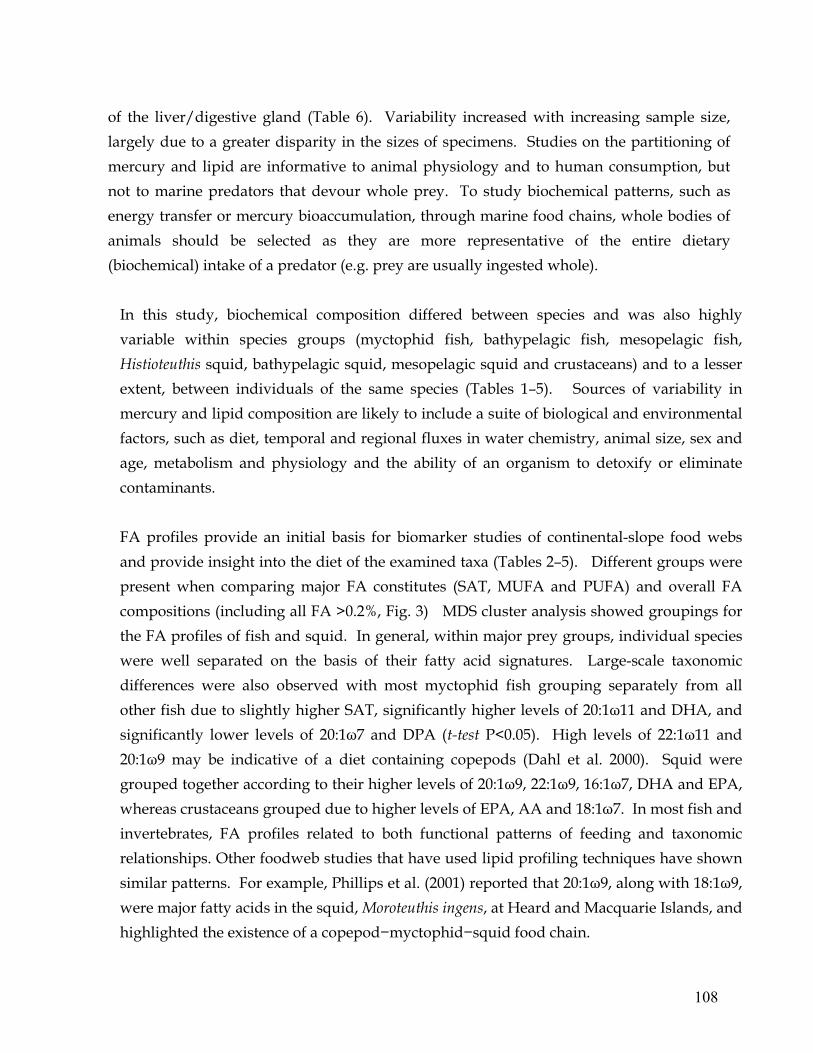
108

of the liver/digestive gland (Table 6). Variability increased with increasing sample size, largely due to a greater disparity in the sizes of specimens. Studies on the partitioning of mercury and lipid are informative to animal physiology and to human consumption, but not to marine predators that devour whole prey. To study biochemical patterns, such as energy transfer or mercury bioaccumulation, through marine food chains, whole bodies of animals should be selected as they are more representative of the entire dietary (biochemical) intake of a predator (e.g. prey are usually ingested whole).

In this study, biochemical composition differed between species and was also highly variable within species groups (myctophid fish, bathypelagic fish, mesopelagic fish, Histioteuthis squid, bathypelagic squid, mesopelagic squid and crustaceans) and to a lesser extent, between individuals of the same species (Tables 1–5). Sources of variability in mercury and lipid composition are likely to include a suite of biological and environmental factors, such as diet, temporal and regional fluxes in water chemistry, animal size, sex and age, metabolism and physiology and the ability of an organism to detoxify or eliminate contaminants. FA profiles provide an initial basis for biomarker studies of continental-slope food webs and provide insight into the diet of the examined taxa (Tables 2–5). Different groups were present when comparing major FA constitutes (SAT, MUFA and PUFA) and overall FA compositions (including all FA >0.2%, Fig. 3) MDS cluster analysis showed groupings for the FA profiles of fish and squid. In general, within major prey groups, individual species were well separated on the basis of their fatty acid signatures. Large-scale taxonomic differences were also observed with most myctophid fish grouping separately from all other fish due to slightly higher SAT, significantly higher levels of 20:1ω11 and DHA, and significantly lower levels of 20:1ω7 and DPA (t-test P<0.05). High levels of 22:1ω11 and 20:1ω9 may be indicative of a diet containing copepods (Dahl et al. 2000). Squid were grouped together according to their higher levels of 20:1ω9, 22:1ω9, 16:1ω7, DHA and EPA, whereas crustaceans grouped due to higher levels of EPA, AA and 18:1ω7. In most fish and invertebrates, FA profiles related to both functional patterns of feeding and taxonomic relationships. Other foodweb studies that have used lipid profiling techniques have shown similar patterns. For example, Phillips et al. (2001) reported that 20:1ω9, along with 18:1ω9, were major fatty acids in the squid, Moroteuthis ingens, at Heard and Macquarie Islands, and highlighted the existence of a copepod−myctophid−squid food chain.

109

Table 4.7 Predictor fatty acids (FA) for various prey groupings as identified by discriminant function analysis

Prey group Predictor FA (major) Minor and non-predictor FA

Fish, myctophids 20:1ω11, 24:1ω9, 16:0, 18:1ω7, 22:1ω9, 20:4ω6, 20:1ω7 mesopelagic bathypelagic

16:1ω7, 16:0, 18 :1ω9, 20:4ω3, 14 :0 22:4ω3, 20:1ω9, 22:1ω11, 20:2ω6

22:6ω3, 22:5ω3, 20:5ω3, 22:1ω9

Squid, mesopelagic bathypelagic

22:6ω3, 22:1ω9 20:1ω7, 20:1ω9, 18:1ω7, 18:0

24:1, 20:2ω6, 22:4ω6, 22:4ω3, 16:1ω7 22:4ω3, 18:2ω6, 24:1

Octopus 20:5ω3, 22:6ω3, 20:1ω7 14:0, 16:1ω7, 18:1ω9, 22:1ω11, 24:1, 22:4ω3 Crustaceans 20:4ω6, 22:5ω3, 20:5ω3, 18:1ω7, 22:1ω9, 22:6ω3 16:0, 18:0, 22:1ω11, 18:4ω3, 22:4ω3,

Figure 4.3 Principle component analysis (PCA) of all FA for all prey species. ● cephalopods, fish, ▲myctophid fish,* crustaceans. (MDS stress = 0.16). DPA, docosapentaenoic acid; EPA, eicosapentaenoic acid; DHA, docosahexaenoic acid

Discriminant function analysis (DFA) indicated the best ‘marker’ fatty acids for each prey

group (Table 7). When treated separately, MDS cluster analysis produced several

groupings within the prey groups of squid and fish (Fig. 4), especially in the relative

proportions of PUFA and MUFA. The choice of cut-off point that defined groupings is

110

Nansenia spTubbia tasmanicaChauliodus sloani

Nemichthy s spLepidorhy nchus denticulatus

Scopelosaurus spWoodsia mey erwaarden

Apogonops anomalusArgy ropelecus gigasMaurolucus australis

Parspasia kapuaMacraronus nov aezelandia

Stomias boaPhotichthy s argenteus

Sy stellaspis debilisSergia potensEuphausia sp

Nototodarus gouldiDiaphus metoploclampus

Nannobrachium spEmmelichthy s nitidus

Sy mbolophorus boopsElectrona paucirastra

Lampany ctus australisProtomy ctophum normari

Thy rsites atunDiaphus danae

Hy gophum hanseniDiaphus hudsoni

Sy mbolophorus barnardiElectrona rossi

Lampichthy s procerusMetelectrona v entralisTeuthowenia pellucidaHistioteuthis atlantica

Octopus spSlosarczkov ia circumantarctica

Octopoteithis megapteraMastiogoteuthis idioteithis

Sepiolidae spHistioteuthis macrohista

Heliocranchia pf ef f eriAncistrocheirus lesueuri

Ly coteuthis lorigeraMastiogoteuthis sp

Acanthephy ra spCoelorichus f asciatus

Notacanthus sexspinisAstronesthes sp

Epigonus robustusWinteria telescopaEpigonus lenimen

Bathy lagus antarcticusTodarodes f ilippov a

Figure 4.4 Hierarchical cluster dendogram based on Bray-Curtis similarity (complete linkage) for the average FA composition of 54 prey species, collected from continental slope waters off south-eastern Australia. Symbols refer to prey groups: ▲ myctophids fish; other fish; ● squid; *crustaceans.

111

somewhat arbitrary, but comparison between the cluster results and the biological and ecological information available enables a useful basis for a description of the different feeding patterns observed. Assuming that the dietary differences attributed to each of these trophic guilds was great enough to be reflected in variations in dietary fatty acids, then species with similar diets, and therefore fatty acid compositions, should theoretically group together. Summary Investigating the biochemical properties of mid-trophic prey groups, including fish and invertebrates, can provide invaluable insight into commonly overlooked aspects of the marine ecosystem. Specifically, the data reported here will have application in wider trophodynamic studies for demersal and temperate Australian food chains, particularly for top-level predators. It will also provide insight into metabolic processes, life-history strategies, habitat usage and buoyancy mechanisms of these documented species. Lipids are the currency by which energy is transferred from lower to higher trophic levels. It is this transfer of lipids, particularly the constituent fatty acids that can be traced from prey to predator elucidating dietary relationships. In this study, some distinct differences in the FA composition of the examined taxa allowed for their separation, indicating that FA profiles can be useful as biomarkers in demersal food web studies. Likewise, species differences in mercury concentrations were related to differences in size, habitat and feeding strategies, and therefore, can be used to delineate feeding relationships and transfer patterns within the foodweb. However, assessing the diet and foraging ecology of a species using contaminant or fatty acid tracers requires more than the comparison of predators and potential prey profiles. It necessitates knowledge of various factors, including habitat, physiology and general biology of a species. Future research should investigate the extent which such variables influence lipid and mercury dynamics. This study represents the first major study using lipid and mercury tracers to investigate broad trophic relationships of marine organisms on the continental shelf of southeastern Australia. For most species examined, this is the first such biochemical data. The mid-trophic species selected in this study, including commercial and non-commercial species, are critically important owing to their role in energy and contaminant transfer and bioavailability. The breadth of prey and their chemotaxonomic separation are also highly

112

relevant, given the general preference for dietary studies to investigate predators occupying only the higher trophic levels. Increasingly, management approaches are assessing ecosystem function and health and include the use of whole ecosystem and dynamic system models. Good examples are the Ecopath (with Ecosim or Ecotracer) framework (Christensen and Walters 2004) and biogeochemical models such as ATLANTIS (Fulton et al. 2004). The mid-trophic prey compositional data presented in this study may be useful to establish new models, particularly in tracking energy transfer, contaminant bioaccumulation, and complex food-web dynamics.

113

5

DIET OF DEMERSAL CHONDRICHTHYANS AS INFERED BY SIGNATURE FATTY ACID PROFILES AND STOMACH CONTENTS

114

CHAPTER 5

DIET OF DEMERSAL CHONDRICHTHYANS AS INFERED BY

SIGNATURE FATTY ACID PROFILES AND STOMACH CONTENTS

ABSTRACT Assessing the diet and trophic relationships between top-level predators and their prey is essential for understanding the dynamics of marine ecosystems, however this has been challenging, with many biases associated with traditional stomach analyses. Here, the diet of 16 demersal shark species, collected as bycatch in waters off south eastern Australia was examined using complementary signature fatty acids and traditional stomach content techniques. Among all species, 59.2 % of all stomachs were empty, with higher occurrence in many mid-slope species. 41 prey taxa were identified, including mostly a mixture of bathypelagic and mesopelagic fish and cephalopods. Differences were observed in feeding histories with increased consumption of crustaceans in upper-slope species and in chimaeras. Common prey taxa amongst all sharks were myctophid fish, Histioteuthis squid and natant decapods. Using multidimensional scaling (MDS) analysis, we determined the extent of variability in the diet composition within each shark species by grouping fatty acid profiles of shark tissues with profiles of local prey fish, cephalopods and crustaceans. In general, the signature FA approach supported the findings obtained by stomach content analysis emphasising significant differences between the diets of sharks and chimaeras. ANOSIM results indicated that there are significant differences in dietary composition between some species while amongst co-existing sharks there is degree of diet overlap. As a complementary method, the signature FA approach provides a broad representation of the diet of chondrichthyans, particularly where there may be some degree of specialisation and a magnitude of geographical or temporal separation. The FA approach is valuable where sample numbers are likely to be low, such as for these deep-sea and threatened organisms.

115

5.1 INTRODUCTION Chondrichthyans occupy a significant ecological niche as top predators in the marine environment, potentially regulating, through predation, the size and dynamics of their prey populations. Understanding competitive and predatory processes is thus necessary to gain insight into the role sharks play in influencing niche, community and food web structure, and ultimately ecosystem dynamics. Worldwide, demersal sharks have been previously described as 'opportunistic' feeders consuming mainly fish, cephalopods and crustaceans depending on seasonal and local opportunity (Wetherbee & Cortés 2004). Given, however, that the supporting data are limited, especially for certain species and regions, and that little is known about the behavior of sharks at sea or the choices they make in prey selection, this description may be an oversimplification. To date, the majority of dietary studies of sharks have used stomach content analyses where high occurrences of empty (or everted) stomachs, few prey items per stomach, advanced state of digestion, and differential digestion rates of particular prey groups (Pierce & Boyle 1991; Hyslop 1980) have meant that excessively large sample sizes are needed to gain quantitative data. While these studies offer a taxonomic description of a predators diet, they often overestimate certain prey groups and provide only a ‘snap-shot’ of the actual diet. Thus, there is a need to incorporate alternative methodologies with more rigorous and quantitative options. Lipid ‘biomarker’ approaches have been used to study the diets of a variety of low-order (eg. decapods, Virtue et al. 1993) and high-order predators (including: seabirds, Budge & Iverson 2003; mammals, Bradshaw et al. 2003; cephalopods, Phillips et al. 2001; and fish, Drazen et al. 2009). Lipids are fundamentally linked with key physiological and biochemical processes and are thus integral to ecosystem functioning. They are grouped according to their mobility and chemical properties, which include structurally simple fatty acids (FA) and the more complex triacylglycerols (TAG), wax esters (WE), glycolipids, phospholipids (PL) and sterols (ST). Determining the amount and composition of specific lipid classes within certain animal tissues can give an insight into metabolic processes at an individual and community level (Parrish et al. 2000). Numerous studies have demonstrated that specific FA patterns are passed from prey to predator near the bottom of the food web (Sargent et al. 1988; Graeve et al. 1994, Kirsch et al. 1998) and that the fatty acid composition of zooplankton directly influences the fatty acid composition of high order predators such as marine mammals (Budge & Iverson 2003). The development of lipid biomarker approaches to study diet is based on FA profiles specific to some organisms

116

and is coupled with a limited capability to synthesize some fatty acids (Darlsgaard et al. 2003). For example, many marine organisms lack the de novo ability to produce polyunsaturated fatty acids (PUFA) and hence rely on a dietary supply (Sargent 1976). Simplified, the basis of this technique is best explained in the simple, yet familiar statement, ‘you are what you eat.’ A large number of studies have explored lipid composition of both muscle and liver tissue in a range of demersal sharks (Bakes & Nichols 1995, Wetherbee & Nichols 2000; Økland et al. 2005), but most have been conducted with a focus on their use for human nutrition and/or by-product development. Signature fatty acid analyses of the muscle and liver of sleeper sharks (Somniosus pacificus) have been used to demonstrate a trophic relationship with planktivores, and that these sharks consume large amounts of blubber derived from baleen whales (Schaufler et al. 2005). No other studies that have used lipid and fatty acid markers as a tool to investigate diet in shark. In this study we combine the use of both traditional stomach analysis together with the biomarker lipid approach to examine the diet of 16 species of sharks. Our aim is to better understand the trophodynamics and community structure of the demersal chondrichthyan assemblages. We make inferences on the usage of FA profiles, and note areas of future research in regards to the wider application of FA profiling techniques in determining the feeding histories in other shark and chimaera species.

5.2 METHODS Sample collection

A total of 404 sharks of 16 species (families: Squalidae, Dalatiidae, Centrophoridae, Somniosidae, Etmopteridae, Chimaeridae, Rhinochimaeridae, Scyliorhinidae and Hexanchidae) were taken opportunistically as bycatch by both local long-line and trawl fishing boats between November 2004 and June 2006 from five sites in continental slope waters exceeding 600 m around eastern and south-eastern Tasmania, and within the Great Australian Bight. Demersal trawl fishing gear consisted of nets with a 35 m headrope, a vertical opening of about 6 m, a footrope length of between 18-25 m and a stretched codend mesh-size of 38 mm. Trawling operations lasted for 3-4 h during both night and day. Trawl depth varied with location and fishing gear but ranged between 500 and 1200 m. Auto-long line fishing gear consisted of a single 1.2 mm diameter braided snoods, 40 cm line attached to a 8 mm mainline at 1.4 m intervals, hooked and baited with squid

117

(Nototodarus gouldi). The line was approximately 3000 m long, positioned at depths ranging from 400-1200 m, along continental slopes and was deployed day and night for 5-6 hours. Upon collection, sharks were identified before the sex, weight (nearest gram) and total length (TL) (nearest 0.5 cm) were determined. All species are named in accordance to the most recent literature (Last and Stevens 2009).

Stomach content

All full stomachs (> stage II) were removed, individually cut open and assigned a fullness rating (0-5 where 5 is completely full) and a level of digestion (1-5 where 5 indicate prey items at an advanced level of digestion and cannot be identified). Empty, everted, or fluid filled stomachs were recorded and discarded upon dissection. Prey items such as hydroids, salps, tunicates and sponges were considered to be incidentally or secondarily ingested and were not included in diet analysis. Contents were sieved, and diagnostic prey items were removed for further identification. Taxonomic resolution was achieved where possible with the aid of identification atlases (Williams & McEldowney 1990, Smale et al. 1995, Clarke 1989; and Furlani et al. unpublished data) and reference collections (CSIRO collections: Dunning 1982, Bulman 1991). After identification, items were separated into broad ecological groupings: mesopelagic, benthic, bathypelagic. Where paired otoliths were present, only 1 was counted to eliminate over-estimation of fish species. Prey groups and prey species were analysed using percent frequency of occurrence (%F), which was calculated as the proportion of samples (with identified prey remains) containing particular prey taxa. Percentage Number index (%NI) was determined as the total number of a particular prey taxa per prey category. The actual number of prey items (for each ecological grouping) were expressed as number of occurrences (N). For C. crepidater, percentage Mass (%M) was determined as the total weight of prey taxa taken from the total weight of all sharks with content. From this, the Percentage Index of Relative Importance (%IRI) was used through the equation: %IRI = 100 (%N + %W) * %F (Pinkas et al. 1971). Niche breadth was quantified for selected shark species, using: B = 1/∑p2j (Levins 1968) determined by the fraction by which food groups and prey items contribute to the diet. Niche breadth was calculated using the broad prey categories described above.

Signature lipid and fatty acid comparisons Fatty acid (FA) profiles of demersal sharks and prey species used in this study are derived from the results of published and unpublished sources. Specifically, the FA profiles of

118

muscle, liver and digestion fluid from the stomach and intestine from 16 demersal shark species (Chapter 2) were compared to 43 species of potential prey fish, 14 squid and 4 crustaceans (Chapter 4) collected in the same region. For representation of low trophic level prey groups, the FA profiles of two polycheates, Tomopteris carpenteri and Vanadis antarctica and one pelagic amphipod, Themisto gaudichaudii were from Phleger et al. (1998). In addition, we included the FA profiles of potential carrion sources (whale blubber from pilot whales: Walters 2005 and sperm whales: Bedard 1998; fur seal blubber: Arnould et al. 2005; squid mantle: Pethybridge (2004). Data used in comparisons were in percent composition form. FA used were those that made up >0.5% and included: 16:0, 18:0, 16:1ω7, 18:1ω7, 18:1ω9, 20:1ω9, 20:1ω11, 22:1ω9, 22:1ω11, 24:1ω9, 20:4ω6, 20:5ω3 (EPA), 22:6ω3 (DHA).

Statistical analysis Multivariate statistics were used to analyze differences in total FA composition. Stepwise linear discriminant function analysis (DFA) using cross-validation was used to identify those FA (predictors) most responsible for group differences based on FA profiles. Separate functions were estimated to predict the group-membership of the tissues (muscle, liver and digestive fluids of the stomach and intestine combined) for each shark species. For the prey data, FA predictors were predetermined (Chapter 4) and were based on the lowest taxonomic level that provided clear separations using DFA. Results from this predictive functions were applied to the tissues of individual shark species and based on discriminant scores we classified shark tissues into one or more of the seven prey groups. Because of the small sample size, the number of FA included in the DFA was limited to FA found in greater than trace amounts (>0.5%) and that exhibited a large mean difference between groups. Non-parametric multi-dimensional scaling (MDS, Krusckall loss function) scatter plots (Bray-Curtis similarity dendrograms) were also used to assess groupings within the dataset. This allowed for the identification of potential prey that most closely resembled the FA composition of sharks. Statistical treatment of the data entailed the application of two-tailed t-tests (assuming unequal variance) to test for significant (p<0.05; 95% confidence interval) differences among samples. This included assessing the variations in FA composition (ANOVA). Analysis of similarity (ANOSIM) was performed on the distance matrix using multiple permutations. Pairwise ANOSIM was used to determine which levels differed within a significant fixed effect (P-value< 0.05). The ANOSIM-R value indicated the extent to which the groups

119

differed (R> 0.75: well separated groups; R = 0.50 – 0.75: separated but overlapping groups; 0.25 – 0.50: separated but strongly overlapping groups; R <0.25: barely separated groups). ANOSIM and MDS analyses were performed with PRIMERv5. Between and within species and group variation was investigated using SPSS for Macintosh (SPSS Inc Chicago Illinios).

5.3 RESULTS

Stomach analysis

In total, 41 prey taxa (including 13 cephalopods, 17 teleost, 5 crustaceans, 2 mammals, 2

elasmobranchs, 1 gastropoda, and 1 polycheate) were identified for all shark species and

across all sites in the study (Tables 5.2 and 5.3). Of all stomachs analysed, 59% were empty,

with as high as 100% in Rhinochimaera pacifica and 92% in Centrophorus zeehaani. Stomachs

with contents, generally had a medium state of digestion (digestive stage 1–3), stomach

fullness (mean 1.6), and 78% of all stomachs with identifiable hard remains contained only

one prey item. No one prey species (or genera) dominated the diet of any one species,

however for most sharks, of those containing identifiable prey, teleosts and cephalopods

were most commonly identified as the primary prey groups. In 12 of the 16 shark species

examined, fish were consumed. 26% of all prey items were classified as unidentified. The

most abundant prey groups present in the diet across the study area were mesopelagic fish

and bathypelagic cephalopods. Dominant taxa consisted of Histioteuthis squid, myctophid

fish (Electrona spp and Diaphus danae), other squid (Teuthowaenia pellucida and

Ancistrocheirus lesueuri), and other fish (Epigonus lenimen and Bathylagus spp). Across all

demersal shark species, there was no recording of truly benthic fish species although

several octopod and cephalopod species were identified, including Vampyroteuthis infernalis

and an unknown Sepiolidae species. Crustacean remains were identified in relatively few

stomachs and were found in a highly digested state in which most could not be identified

beyond broad group categories. Of those that were identified, natant decapods and Segia

potens were present in all mid-slope species with sample sizes greater than 30. In larger

sharks (Proscymnodon plunketi, Dalatias licha, and Notorynchus cepedianus), portions of

dogfish shark, seal and whale blubber (presumably carrion) were observed. In shelf and

upper-slope Squalidae species, mesopelagic fish dominated the diet and the consumption of

crustaceans was higher than for dogfish species inhabiting mid-slope waters of Tasmania.

Most prey species examined in upper-slope species were not observed in mid-slope sharks,

120

Table 5.1 Diet composition of ten demersal shark species in terms of number (N), numerical importance (%NI), and frequency of occurrence (%F) for the major prey taxa and identifiable dietary categories

Species Code

Centroselachus crepidater

Etm

opterus baxteri

D

eania calcea

Squalus

acanthias

Squalus m

itsukurii

Squalus m

egalops

Proscymnodon

plunketi

Dalatias licha

Figaro boardm

ani

Chimaera

lignaria

Total No. stomachs 58 98 47 43 37 15 7 5 12 22 % stomachs empty/inverted 47.5 68.3 61.7 51.1 69 50 28 0 0 37 Total prey No. 46 37 25 26 14 9 9 6 22 18 Mean No. prey per stomach *

1.5 1.2 1.4 1.2 1.1 1.3 1.8 1.2 1.8 1.3

Mean stomach fullness * 2.9 1.9 2.3 4.3 2.6 2.2 3.5 4.2 3 2.6 Mean state of digestion * 3.5 4.2 3.9 2.3 3.0 3.2 3 3.6 3.5 3 Niche breadth ** (7) 4.9 (7) 4.3 (5) 3.4 (4) 2.8 - - - - - -

Major Prey Taxa/Groupings

N %NI %F %W %IRI N %NI %F N %NI %F N %NI %F N N N N N N

CEPHALOPODA Unidentified Benthic Cephalopods Octopoda Vampyroteuthis infernalis Sepiolidae spp. Bathypelagic Cephalopods Ancistrocheirus lesueuri Chiroteuthis sp. Histioteuthis spp. Histioteuthis macrohista Histioteuthis c.f atlantica Teuthowaenia pellucida # Mesopelagic Cephalopods Lycoteuthis lorigora Todarodes fillipovae Moroteuthis robsoni Nototodarus gouldi

Ha Tp

Tf Mr Mg

20 34.4 5 8.6 3.4 1 1.7 1 1.7

- 15.5 2 3.4 1 1.7 3 5.1

- 1 1.7 2 3.4 6.9 2 3.4 1 1.7 1 1.7

-

43.410.8 4.3 2.2 2.2 -

19.5 4.3 2.2 6.5 -

2.2 4.3 10.8 4.3 2.2 2.2 -

26.1 5.7 2.1 1.5 0.6 -

8.4 1.3 0.6 2.4 -

1.9 2.2 9.9 3.1 4.6 2.3 -

40.1 2.3 0.4 0.3 0.2 -

17.7 0.7 0.1 0.2 -

0.3 0.9 6.9 1.1 0.5 0.3 -

15 3 - 2 - 1 - 3 2 2 - - - 2 -

15.3 3.1 2.0 -

2.0 -

8.2 1.0 -

3.1 2.0 2.0 -

2.0 - -

2.0 -

40.5 8.1 5.4 -

5.4 -

21.6 2.7 -

8.1 8.1 5.4 -

5.4 - -

5.4 -

8 1 - - - 1 1 1 - 1 1 - 1 1 -

17.0 2.1 0.0 - - -

10.6 2.1 2.1 2.1 -

2.1 2.1 4.2 -

2.1 2.1 -

32.0 4.0 0.0 - - -

20.0 4.0 4.0 4.0 -

4.0 4.0 8.0 -

4.0 4.0 -

6 2 - - 2 - - - - - - - - - 1 1

13.9 4.6 4.6 - -

4.6 0.0 - - - - - -

4.6 - -

2.3 2.3

23.1 7.7 7.7 - -

7.7 0.0 - - - - - -

7.7 - -

3.8 3.8

4 2 - 1 - 1 - - - - - - - - - - - -

2 1 - - - 1 - - - - - - - - - - - -

2 - - - - - - - - 1 - - - - 1 - - -

0 - - - - - - - - - - - - - - - - -

17 8 4 1 1 - - - - - - - - - - 1 2

0 - - - - - - - - - - - - - - - - -

121

Table 5.1 continued

Species Code

Centroselachus

crepidater

Etm

opterus baxteri

D

eania calcea

Squalus

acanthias

Squalus mitsukurii

Squalus megalops

Proscymnodon

plunketi

Dalatias licha

Figaro boardmani

Chimaera lignaria

TELEOSTS Unidentified Bathypelagic Bathylagus spp Epigonus lenimen Ceratioidei sp Hoplostethus atlanticus # Howella sp Tetragonurus cuvieri Argentina australiae Mesopelagic Arripis georgianus Chauliodus stoani Myctophidae unid spp # Diaphus danae # Lampanyctus australis # Electrona spp. Photichthys argenteus # Nansenia sp. Emmelichthys nitidus Thyrsites spp.

B El - -

H Tc Aa

Cs

Dd La

Pa N En Ta

19 32.7 6 10.3 6.9 1 1.7 1 1.7 1 1.7

- - -

1 1.7 15.5

- 2 3.4 2 3.4

- -

2 3.4 2 3.4 1 1.7

- -

41.3 13.0 8.7 2.2 2.2 2.2

2.2 19.5

- 4.3 4.3 - -

4.3 4.3 2.2 - -

60.8 23.5 14.0 4.0 4.2 1.9 - - -

2.9 23.3

- 4.2 5.9 - -

4.7 3.8 1.9 - -

67.6 11.4 4.7 0.3 0.3 0.2 - - -

0.3 19.6

- 0.9 1.0 - -

0.9 0.8 0.2 - -

17 5 2 1 - 1 1 2 - - - 2 - 1 - 1 1 - -

17.3 5.1 7.1 2.0 1.0 -

1.0 1.0 2.0 -

5.1 - -

2.0 -

1.0 -

1.0 1.0 - -

45.9 13.5 18.9 5.4 2.7 -

2.7 2.7 5.4 -

13.5 - -

5.4 -

2.7 -

2.7 2.7 - -

13 3 - 1 - - - - 1 - - 4 2 - 1 - 1 - -

27.6 6.4 2.1 -

2.1 - - - -

2.1 17.0

- -

8.5 4.2 -

2.1 -

2.1 - -

52.0 12.0 8.0 -

4.0 - - - -

4.0 32.0

- -

16.0 8.0 -

4.0 -

4.0 - -

16 7 - - - - - - - 2 - 3 - - - - - 3 1

37.2 16.3 0.0 - - - - - - -

20.9 4.6 -

7.0 - - - - -

7.0 2.3

61.5 26.9 0.0 - - - - - - -

34.6 7.7 -

11.5 - - - - -

11.5 3.8

6 2 - - - - - - - - - 1 - 1 - - - - - 2 1

4 2 - - - - - - - - - 1 - - - - - - - - -

6 3 - - - - - - 1 - - - - - - - - - - - -

4 2 - 1 - - 1 - - - - - - - - - - - - - -

3 1 - - - - - - - - - - - 1 - - - - - 1 -

3 2 - 1 - - - - - - - - - - - - - - - - -

CRUSTACEA Unidentified Segia potens # Natant unid spp. Euphausii unid sp Amphipoda Homolodromiidae (Crabs)

Sp

E

6 10.3 2 3.4 3 5.1 1 1.7

- - -

13.0 4.3 6.5 4.3 - - -

5.1 2.0 2.6 0.6 - - -

2.9 0.4 0.8 0.1 - - -

4 1 1 1 1 - -

4.1 1.0 1.0 1.0 1.0 - -

10.8 2.7 2.7 2.7 2.7 - -

4 2 1 1 - - -

8.5 4.2 2.1 2.1 - - -

16.0 8.0 4.0 4.0 - - -

4 1 - 1 - - 2

9.3 2.3 -

2.3 - -

4.6

15.4 3.8 -

3.8 - -

7.7

3 2 - - - - 1

3 1 - 1 - - 1

0 - - - - - -

0 - - - - - -

2 1 - - - 1 -

8 3 - - 1 1 3

OTHER Elasmobranchs Mammalians – seal, cetacean Gastropoda Polycheates

1 1.7 -

1 1.7 - -

.

2.2 -

2.2 - -

5.2 -

5.2 - -

0.2 -

0.2 - -

1 1 - - -

1.0 1.0 - - -

2.7 2.7 - - -

- - - -

0.0 - - - -

0.0 - - - -

- - - - -

0.0 - - - -

0.0 - - - -

1 - - 1 -

1 - - - 1

1 - 1 - -

2 1 1 - -

0 - - - -

3 - - 2 1

Nematode parasites 4 5 2 * Not including those stomachs that were empty. **Niche breadth includes all prey groups as well as dominant species (%F>10). N = Number of otoliths, NI =Numerical Importance of each otolith, %FO = Percent frequency occurrence, %W = Percentage mass, and %IRI = index of relative importance on a percent basis. # = abundant around Tasmania.

122

Table 5.2 Dietary information for shark species examined with small samples sizes Species N % Empty Mean SF SOD Major prey groups identified

Centropurus zeehaani 38 92.1 2 3.9 Fish, cephalopod

Centrosymnus owastoni 2 50 2 4 Cephalopods

Centrosymnus coelopsis 2 100 1.2 5 -

Apristurus sinensis 6 83.4 3 3 Crustacea

Rhinochimeara pacifica 8 100 1.5 5 -

Notorynchus cepedianus 2 0 3.4 2.6 Mammal – seal , fish Stomach Fullness (SF) and State of Digestion (SOD) are indices ranging from 0-5 where 0 is empty or digested fluids, respectively *non solid prey items, but fluid present.

such as the mesopelagic fish Emmelichthys nitidus and Thyrsites sp. and arrow squid, N.

gouldi. Crab species were found only in the stomachs of Squalus dogfish sharks and

chimaera, Chimaera lignaria. Unlike all other shark species, all individuals of Figaro

broadmani had prey remains, with cephalopods accounting for 77% of all prey. Stomach

contents of Chimaera contained crustaceans (44%), including amphipods and crabs in

addition to gastropods and polycheates. Few commercially important species were

identified, with the exceptions of orange roughy, H. atlanticus, barracouta, Thyrsites atun

and arrow squid, N. gouldi.

In C. crepidater, additional indices of diet (%weight, %IRI) were used to reduce and

underline associated biases. When weight was taken into consideration, fish were a more

dominant prey group than cephalopods. The diversity of fish remains in stomachs and the

large numbers of empty stomachs taken at each site was directly related to sample size (R2 =

0.87). Due to the limited number of identified species and small sample size at some

locations, no spatial (between sites), seasonal or interannual data could be statistically

tested.

Principal component analyses of demersal sharks and potential prey Tissue choice and general patterns in FA profiles between all shark and prey species FA profiles of the muscle, liver and digestive tissues of demersal sharks (reported in Chapter 2) and of potential whole prey species (Chapter 4) were compared using non-

123

parametric multi-dimensional scaling (MDS) and discriminant analysis (DFA). Regardless of species, shark liver and muscle tissues grouped together separately, whereas stomach and intestine fluid samples grouped with various prey species (MDS, Fig. 5.1). PCA analyses showed that the FA, 18:1ω9, 22:6ω3 explained most of the PC1 (x-axis) variance (47.3%), whereas 18:1ω9, 20:5ω3, 22:2ω11, 20:1ω9 and 16:0 explained 17.5% of the PC2 (y-axis) variance. To demonstrate the degree of bias in allocating potential prey groups according to the muscle and liver tissues, the significant and main predictor FA of each tissue were tested against the predictor FA of prey groupings (Table 5.3). The muscle is considered slightly biased in grouping with PUFA rich organism including cephalopods (ANOSIM-R = 0.64), crustaceans and amphipods. In contrast, shark liver more closely resembled the FA profile of numerous fish species (ANOSIM-R = 0.47–0.53), in addition to the blubber of higher-order fish-consuming mammals (fur seal, pilot whale and sperm whale). A greater inclusion of potential prey groups became apparent when less dominated, tissue-member FA were used, in addition to those FA that equally occurred in both tissues (Table 5.3). Individual FA that are typically not of dietary origin included 16:0 found predominantly in the muscle and 18:1ω9 and 16:1ω7 in the liver. In contrast, FA that are of exclusive or major dietary origin included 20:5ω3 in the muscle and 22:1ω11 and 14:0 in the liver.

Table 5.3 Comparisons between muscle and liver FA composition and potential biases in determining prey groups

LDA Predictor FA Potential prey species

Muscle 20:4ω6*, 22:6ω3*, 16:0, 18:0, 22:4ω6, 20:5ω3, 22:5ω3,

Crustaceans*, octopus, MP squid MP and BP fish, squid, crustaceans, amphipods, echinoderms,

Liver 18:1ω9*, 20:1ω9*, 22:1ω11/13*, 20:1ω7, 22:1ω9, 24:1, 14:0, 16:1ω7,

MP and BP fish*, BP squid*, mammal blubber, copepods Fish, squid, octopus, myctophid fish

Co-occurring FA (muscle and liver)

17:1ω8/16:1ω9, 18:1ω7, 20:2ω6, 22:4ω3

BP squid*, crustaceans, whale blubber, BP fish

Significant FA (p<0.01) as determined by linear discriminant analysis (LDA) and tested by ANOVA. Other FA were seen as influential but less significant (p<0.05). Co-joint FA refer to those that were nether dominant in the muscle or liver, but varied significantly between shark species (ANOVA, P<0.01). Underlined prey groups represent those that grouped with the shark tissue as determined by ANOSIM (ANOSIM-R <0.75). Individual FA presented in grey are not typically of dietary origin, whereas FA presented in bold are of exclusive or major dietary origin. MP – Mesopelagic, BP – Bathypelagic

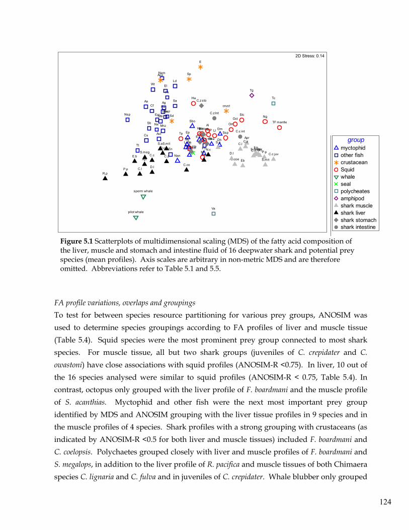
124

DdDh

DmEp

Er

Hh

La

LpMv

Nan

Pn

Sba

Sbo

Ta

En

Aa

Nsp

Ag

Sb

Tt

Pk

Sa

Nem

Wm

Mnz

Ld

Ma

Pa

Cs

Bsp

Cf

Wt

Epi

El

Ns

Ast

Asp Sp

E

Sd

Ha

Hm

Slc Ng

LlHpOm

Tp

Mi

Msp

Oct

Al

SspTf

Tf

TF mantle

pilot whale

sperm whale

crust

seal

Va

Tc

Tg

Eb

C.cC.c juv

C.coe

C.owP.pD.c

D.l

C.l

Apr

F.b

C.z

S.meg

S.a

S.mitE.b C.c

C.coP.p

D.c

D.lC.lR.p

AprF.bC.z

S.meg

S.aS.mit

N.c

E.b st

E.b int

C.z sto

C.z Int

C.c sto

C.c int

P.p sto

2D Stress: 0.14

groupmyctophidother fishcrustaceanSquidwhalesealpolycheatesamphipodshark muscleshark livershark stomachshark intestine

Figure 5.1 Scatterplots of multidimensional scaling (MDS) of the fatty acid composition of the liver, muscle and stomach and intestine fluid of 16 deepwater shark and potential prey species (mean profiles). Axis scales are arbitrary in non-metric MDS and are therefore omitted. Abbreviations refer to Table 5.1 and 5.5.

FA profile variations, overlaps and groupings To test for between species resource partitioning for various prey groups, ANOSIM was used to determine species groupings according to FA profiles of liver and muscle tissue (Table 5.4). Squid species were the most prominent prey group connected to most shark species. For muscle tissue, all but two shark groups (juveniles of C. crepidater and C. owastoni) have close associations with squid profiles (ANOSIM-R <0.75). In liver, 10 out of the 16 species analysed were similar to squid profiles (ANOSIM-R < 0.75, Table 5.4). In contrast, octopus only grouped with the liver profile of F. boardmani and the muscle profile of S. acanthias. Myctophid and other fish were the next most important prey group identified by MDS and ANOSIM grouping with the liver tissue profiles in 9 species and in the muscle profiles of 4 species. Shark profiles with a strong grouping with crustaceans (as indicated by ANOSIM-R <0.5 for both liver and muscle tissues) included F. boardmani and C. coelopsis. Polychaetes grouped closely with liver and muscle profiles of F. boardmani and S. megalops, in addition to the liver profile of R. pacifica and muscle tissues of both Chimaera species C. lignaria and C. fulva and in juveniles of C. crepidater. Whale blubber only grouped

125

with D. licha (ANOSIM-R = 0.5) which is a shark species with a very short snout and classic cookie cutter teeth. Shark species that had large within tissue variation in their FA profiles (eg. S. acanthias) showed greater inclusion of different prey groups, as did those shark species that had FA profiles which were not well separated from prey groups (F. boardmani, and liver of N. cepedianus).

Comparisons of shark and prey FA profiles To examine potential dietary patterns within selected shark species, FA were identified as adequate predicators of group membership for individual shark tissues using DFA. Shark tissue predictor FA were then matched to the predictor FA of various prey groups (as determined in Chapter 4). The resulting discriminant functions were used to predict the prey-group membership of the individual tissues of the 16 shark and chimaera species analysed (Table 5.5). MDS analyses of individual shark species were also used to investigate potential dietary differences and dominant shifts in the diet between shark species (Fig. 5.3). In all species analysed, PC1 (x-axis) accounted for the largest variations (37.6 % in S. acanthias – 53.1% in C. crepidater) largely explained by variations in 22:6ω3, 20:5ω3 and 16:0. PC2 (y-axis) accounted for less variation (15.5 – 30.2%) largely due to changes in 18:1ω9 and 22:5ω3. Due to the conjectures associated with linking the FA profiles of muscle and liver tissues in sharks (described above), clusters were established between the profile groupings of muscle and liver. Where data was available, clusters included the FA profiles of the stomach and intestine fluid. For golden dogfish, C. crepidater, the joined cluster grouped mainly with myctophid fish and cephalopod species (Fig. 5.3A), which confirms results from DFA with adults linked to a mix of squid, fish and crustaceans (Table 5.5). Muscle FA profiles of juveniles and adults statistically differed (ANOVA p = 0.02) with higher concentrations of 22:5ω3 and 22:6ω3 and lower concentrations of 16:0 and 18:1ω9 in juveniles (<50 cm TL) than in adults (>69 cm TL). DFA analysis indicated that juveniles have a higher inclusion of crustacean than adults while results from ANOSIM indicated the inclusion of polychaetes in the diet (Table 5.5). For MDS, the liver of 1 specimen of C. crepidater grouped closely to sperm whale blubber while muscle of another specimen grouped closely to mantle tissue of T. filippova, with little similarity between the two recorded by DFA or ANOSIM analyses. The increased inclusion of deep-sea shrimp, Systellaspis debilis, was also noted in the joint profile cluster (Fig. 5.3A). In comparison to C. crepidater, the liver profiles of the lantern dogfish, E. baxteri moved further from whale blubber profiles and were more similar to fish (ANOSIM-R =0.82, Fig.

126

5.3B). Similarly, the muscle of E. baxteri shifted away from squid mantle tissue in addition to crustacean species, and was grouped more with other squid species (ANOSIM-R = 0.81). Digestive tissue profiles centered in the cluster between the liver and muscle and were very similar in profile to that of bathypelagic squid (ANOSIM-R <0.05), confirming findings from DFA. The large MDS cluster between all tissues profiles of E. baxteri included a mix of squid, myctophid fish and two other fish species, barbeled dragonfish from the genus Astronesthes and viper fish, Chauliodus sloani (Cs, Fig 5.3B).

Table 5.4 Between species resource partitioning for prey groups as determined by ANOSIM pairwise tests between multiple prey and shark species.

Prey group Liver Muscle

Myctophid Fish

N. cepedianus**, S. acanthias**, C. coelopsis*, C. zeehaani* , F. boardmani*, F. boardmani*, S. acanthias**, D. licha* C. coelopsis*

Other Fish, MP BP

S. acanthias**, N. cepedianus*, S. megalops*, S. mitsukurii**, C. zeehaani**, C. crepidater *, C. lignaria*

F. boardmani**, S. acanthias*,

Squid, MP

BP

F. boardmani **, N. cepedianus***, S. acanthias*, S. megalops*, S. mitsukurii*

D. calcea*, C. coelopsis**,C. zeehaani*

F. boardmani***, S. acanthias**, S. megalops*, C. zeehaani* A. sinensis**, D. licha**, P. plunketi*, E. Baxter*, D. calcea*, C. lignaria*

Octopus F. boardmani** S. acanthias*

Crustaceans N. cepedianus***,F. boardmani***,C. coelopsis* F. boardmani**, C. coelopsis*, C. zeehaani *, C. lignaria*,

Mammal blubber D. licha**, C. coelopsis **, P. plunketi*

Polychaetes F. boardmani**, R. pacifica*, S. megalops* F. boardmani**, C. crepidater juvenile**, C. fulva*, C. lignaria*, S. megalops*

*** ANOSIM-R = <0.25 ** R = 0.25 – 0.5, * R = 0.5 – 0.75. MP – Mesopelagic, BP – Bathypelagic

127

Table 5.5 Comparisons of predictor FA of shark tissues and prey groups based on linear discriminant analysis (LDA) and confirmed by analysis of similarity (ANOSIM), relative to different combinations of FA. Shark species Tissue Predictor FA in shark tissues Predicted prey groups ANOSIM-R

Inner Upper-slope (0-400)

N. cepedianus Nc Liver 16:1w7*, 16:0*, PUFA*, 20:5w3*, 20:4w6, 22:6w3, 22:4w6, SAT

Myctophid fish*, crustaceans*, BP squid, seal blubber, octopus, <0.26

S. acanthias Sa Liver 24:1, 22:5w3, 18:0 Myctophid fish*, crustaceans*, squid, benthic organisms 0.31

Muscle 20:5w3*, 20:1w9*, MUFA*, 20:4w3*, 22:1 fish*, BP squid*, octopus, crustaceans 0.46–0.54 S. megalops SmegLiver 20:1w9*, 18:0*, 20:2w6, 22:4w3 BP and MP fish*, squid, crustaceans 0.51–0.58 Muscle 22:6w3*,18:2w6 MP squid*, octopus, crustaceans, polychaetes 0.56–0.66

S. mitsukurii 1 Sm Liver 24:1, 22:4w6 BP fish, squid, Myctophid fish, crustaceans, benthic orgs 0.31–0.70

Muscle PUFA Octopus, crustaceans, squid 0.81 Outer Upper-slope (400-650) C. zeehaani Cz Liver 20:4w6*, 16:0, SAT MP fish*, Crustaceans, squid 0.42, 0.69 Muscle SAT, 20:5w3*, 18:0*, 16:0, 16:1w7 Crustaceans*, squid* 0.66 Digestive fluids 16:0*, 18:0, 22:4w6, 22:1w9, 20:1w7 Myctophid Fish, squid, crustaceans 0.32–0.53

F. boardmani Fb Liver 20:5w3*, 14:0*, 22:6w3*, 22:5w3*, 16:1w7, PUFA* Octopus**, squid*, crustaceans*, MP fish, 0.17

0.41

Muscle 16:0, 20:2w6*, 22:6w3 fish, MP squid crustaceans

<0.05 0.25

Mid-slope (650-1200) C. crepidater Cc Liver 20:1w7*, 22:1w9*, 22:4w3 BP squid*, BP fish, crustaceans, octopus, 0.67 Digestive fluids 22:6w3, 16:0, 14:0, 18:1w9 MP fish*, squid, crustaceans <0.05 Muscle 22:6w3 Octopus, crustaceans, MP squid 0.81 C. crepidater Juv. Muscle 22:5w3*, 22:1w9, 22:6w3, Crustaceans*, BP squid, polychaetes 0.50 E. baxteri Eb Liver 24:1*, 20:1w11, 22:1w11/13, 22:1w9 Myctophid fish*, BP squid*, crustaceans 0.82 Muscle 18:1w9 MP fish, benthic organisms, squid 0.81

Digestive fluids 18:1w7*, 22:1w11*, 20:1w9, 20:4w6, 22:4w3, 22:5w3 BP fish*, BP squid*, crustaceans* <0.05

D. calcea Dc Liver 20:1w11*, 16:0* Myctophid fish*, MP fish 0.38 Muscle 22:4w6*, 20:1w9, 22:6w3 BP fish*, squid, crustaceans, octopus 0.69 D. licha Dl Liver 18:1w9*, 18:2w6*, 17:1w8/16:1w9 Whale and seal blubber, BP fish 0.48-0.54

Muscle 20:4w6*, 16:1w7*, 18:1w9 Whale and seal blubber*, MP fish, crustaceans, BP squid 0.49

P. plunketi Pp Liver 18:1w9*, MUFA*, 22:1w9 Fish, mammal blubber, BP squid 0.8 Muscle 16:0, 18:2w6, 22:6w3 MP fish, fish, MP squid, octopus, crustaceans 0.48 Stomach fluids 16:1w7, 14:0, 18:1w9, MUFA Seal blubber* MP fish, squid, fish 0.02–0.19 C. coelopsis Ccoe Liver 17:0*, 18:1w5* Crustaceans, mammal blubber, squid, 0.05, 0.41

Muscle 20:1w7*, 18:1w9 BP squid, MP fish, mammal blubber, benthic organisms, octopus, crustaceans

0.57 0.66

C. owostoni Co Muscle 20:1w9, 22:6w3 BP fish, MP squid, crustaceans, octopus 0.67 A. sinensis Apr Liver 20:4w3**, 14:0*, 20:1w9 MP fish*, squid, BP fish All > 0.90 Muscle 20:1w9*, 16:0*, 22:4w6*, 22:5w3* BP fish*, crustaceans *, BP squid, MP fish 0.38 Chimaeriformes C. lignaria Cl Liver 18:1w7**, 18:1w9* Polychaetes*, crustaceans*, MP fish, BP squid 0.69

Muscle 20:5w3*, 20:4w6*, 18:1w7, 22:4w3,18:2w6

crustaceans**, Octopus*, amphipods, echinoderms, BP squid, polychaetes

0.58 0.71

C. fulva Cf Muscle 16:0, 18:1w7, 20:2w6, 22:4w6 Benthic organisms, BP squid, BP fish 0.55

R. pacifica Rp Liver 22:1w11**, MUFA*, 22:1w9 Copepod food-chain (ophuroids)*, BP fish, crustaceans, BP squid, polychaetes 0.75

1 Distribution of S. mitsukurii extends to both inner and outer upper-slope. Predictor FA represents the most prevalent fatty acids in descending order of dominance as determined by linear discriminant analysis (LDA) classification. ** Signifies specific FA and prey groupings that are of high significance p<0.01 or * moderate significance p<0.05, as determined by LDA and ANOVA. Underlined prey groups represent those most closely associated with the shark tissue FA profiles as determined by ANOSIM. Prey groups underlined and italicized correspond to those that where recognized in ANOSIM but not LDA. The ANOSIM-R value indicates the extent to which the groups differed (R> 0.75: well separated groups; R = 0.50 – 0.75: separated but overlapping groups; 0.25 – 0.50: separated but strongly overlapping groups; R <0.25: barely separated groups). MP - Mesopelagic, BP – Bathypelagic

128

In the piked dogfish, S. acanthias, there were fewer differences between the liver and muscle tissue FA profiles, with higher levels of PUFA found in the liver in comparison to other sharkspecies. Due to this a large shift in the cluster positioning was observed which corresponded to a greater inclusion of squid and mesopelagic fish species, particularly myctophids (Fig. 5.3C). Such results were confirmed by both DFA and ANOSIM with a large overlap in FA profiles between the liver and myctophid fish (ANOSIM-R = 0.31, Table 5.5). Of the other fish, two species that grouped particularly close to the centre of the clustering was the FA profile of barracouta, Thyrsites atun (Ta) and redbait Emmelichthys nitidus (En, Fig. 5.3C). In the gulper shark, C. zeehaani, the FA profiles of the muscle, liver and digestive stomach and intestine fluids significantly differed (DFA, p < 0.01), and thus when tested with prey profiles, the shape of the joint profile cluster changed considerably (Fig 5.3E). Muscle tissue FA profiles grouped most closely to crustaceans (ANOSIM-R = 0.66) while the liver clustered closely to mesopelagic and myctophid fish (ANOSIM-R = 0.43 and 0.72, respectively). The stomach and intestine fluid was close to fish and squid species (DFA, Table 5.5). In the deep-sea chimaera, C. lignaria, the FA grouping of the joint liver and muscle cluster shifted significantly in comparison to other shark species, due to the exclusion of all squid species (Fig. 5.3E) and noticeably there was a greater inclusion of crustaceans and polychaetes profiles to the muscle (Table 5.5). In contrast the liver grouped most with fish (ANOSIM-R = 0.69) and according to DFA, prey-groupings also consisted of echinoderms, crustaceans and bathypelagic squid (Table 5.5). Another large shift in FA profiles of both the muscle and liver was displayed by the sawtail shark, F. boardmani with again a greater inclusion of crustacean species (Fig 5.3F). In comparison to C. lignaria, the cluster produced for F. boardmani has a high inclusion of squid species and there is a much greater influence from whale blubber and to a lesser extent fish species. DFA demonstrated that F. boardmani groups closely to octopus, squid, mesopelagic fish and crustaceans (ANOSIM-R < 0.41, Table 5.5).

129

Figure 5.2 Scatterplots of multidimensional scaling (MDS) based upon the FA composition of various prey species and individual shark species: A) Centroselachus crepidater, B) Etmopterus baxteri, C) Squalus acanthias, D. Chimaera lignaria, E. Centrophorus zeehaani, F. Figaro boardmani. Axis scaled are arbitrary in non-metric MDS and are therefore omitted. Circles around samples indicate the cluster grouping between muscle and liver profiles, and include stomach and intestine fluid where data was available. Arrows indicate significant movement of prey species or prey groups, where arrows moving away from the circled area indicates less inclusion in a sharks diet. Species abbreviations are defined in Table 5.1 – 5.5.

130

Figure 5.3 continued (See previous page).

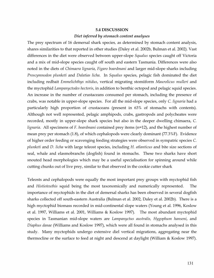
131

5.4 DISCUSSION Diet inferred by stomach content analyses

The prey spectrum of 16 demersal shark species, as determined by stomach content analysis, shares similarities to that reported in other studies (Daley et al. 2002b, Bulman et al. 2002). Vast differences in the diet were observed between upper-slope Squalus species caught off Victoria and a mix of mid-slope species caught off south and eastern Tasmania. Differences were also noted in the diets of Chimaera lignaria, Figaro boardmani and larger mid-slope sharks including Proscymnodon plunketi and Dalatias licha. In Squalus species, pelagic fish dominated the diet including redbait Emmelichthys nitidus, vertical migrating stomiiform Maurolicus mulleri and the myctophid Lampanyctodes hectoris, in addition to benthic octopod and pelagic squid species. An increase in the number of crustaceans consumed per stomach, including the presence of crabs, was notable in upper-slope species. For all the mid-slope species, only C. lignaria had a particularly high proportion of crustaceans (present in 63% of stomachs with contents). Although not well represented, pelagic amphipods, crabs, gastropods and polycheates were recorded, mostly in upper-slope shark species but also in the deeper dwelling chimaera, C. lignaria. All specimens of F. boardmani contained prey items (n=12), and the highest number of mean prey per stomach (1.8), of which cephalopods were clearly dominant (77.3%F). Evidence of higher order feeding or scavenging feeding strategies were observed in sympatric species C. plunketi and D. licha with large teleost species, including H. atlanticus and bite size sections of seal, whale and elasmobranchs (dogfish) found in stomachs. These two sharks have short snouted head morphologies which may be a useful specialisation for spinning around while cutting chunks out of live prey, similar to that observed in the cookie cutter shark Teleosts and cephalopods were equally the most important prey groups with myctophid fish and Histioteuthis squid being the most taxonomically and numerically represented. The importance of myctophids in the diet of demersal sharks has been observed in several dogfish sharks collected off south-eastern Australia (Bulman et al. 2002, Daley et al. 2002b). There is a high myctophid biomass recorded in mid-continental slope waters (Young et al. 1996, Koslow et al. 1997, Williams et al. 2001, Williams & Koslow 1997). The most abundant myctophid species in Tasmanian mid-slope waters are Lampanyctus australis, Hygophum hanseni, and Diaphus danae (Williams and Koslow 1997), which were all found in stomachs analysed in this study. Many myctophids undergo extensive diel vertical migrations, aggregating near the thermocline or the surface to feed at night and descend at daylight (William & Koslow 1997).

132

The presence of these species in stomachs indicates that demersal sharks may undergo vertical migration or are likely to feed on these species during the day when they are found at their maximum depth range. Of the bathypelagic fish, the genus Bathylagus and the demersal argentinid Argentina australidae, both of which are abundant around Tasmania (Young et al. 1996) were also found. Of the cephalopods, Histioteuthis atlantica and Teuthowaenia pellicida were common in the diet of mid-slope species, and are widely distributed within deepwater masses and continental slopes (William & Koslow 1997). The bathypelagic squid, Vampyroteuthis infernalis, which is found at depths between 600 – 1200 m was found in three shark species including C. crepidater, E. baxteri and F. broadmani. Gould’s squid, Nototodarus gouldi is abundant over the continental shelf from 50 m to 200 m (Winstanley et al. 1983), and was present in the stomach contents of S. acanthias and F. boardmani. As in other dietary studies, a high occurrence of empty stomachs and few stomachs containing more than a single prey item, representing the last meal only, illustrates an inherent difficulty associated with stomach content analyses. Such patterns in stomach contents could be indicative of the opportunistic feeding nature of sharks (Mauchline & Gordon 1986) and infers that demersal sharks feed infrequently. In the present study, much of the stomach content material was unable to be taxonomically resolved to prey species and many prey occurrences were reported as unidentified fish, cephalopods and crustaceans. This was primarily due to the absence and/or deterioration of hard prey items, and is a bias, common to many dietary studies (Pierce & Boyle 1991). Additionally, the relatively low occurrences, or absence of known abundant species (eg. Lampanyctus intricarius in southeastern Tasmania) indicate that some species are poorly represented and that a much broader representation of prey is likely to contribute to the diet of demersal sharks. Furthermore, differential digestion rates between prey groups and species within the stomach, particularly the long retention time of squid beaks (Bigg & Fawcett 1985), lead to difficulties when attempting to quantify the importance of a particular prey group. Hence, both cephalopods, and to a lesser degree crustaceans may be over represented. In an attempt to overcome these issues, we tested the usefulness of the FA signature method in investigating the diet of sharks.

Diet as inferred by FA tissue profiles A major aim of the present study was to utilize FA profiles to ascertain the diet of deepwater shark and chimaera species. This approach has been used in an increasing number of dietary

133

studies of high-order marine predators (eg. Budge & Iverson 2003; Bradshaw et al. 2003; Phillips et al. 2001, 2003), largely as a complementary method. As demonstrated in Chapter 2, some caution needs to be taken when drawing dietary conclusions from the signature FA profile of individual chondrichthyan tissues. This is particularly true as there are clear differences in the FA profiles of muscle and liver tissue, and that digestive stomach and intestine fluid FA profiles lie in between indicating the mobilisation of various FA from the diet. When the mean tissue FA profiles of all chondrichthyans species analysed in this study were compared to potential prey (reported in Chapter 4), it was clear that digestive fluids from the stomach and intestine, aligned most closely to specific prey species (Fig. 5.1). Such results were expected as fluids from these tissues represent the most recent feeding event before FA are mobilised and transported to other tissues around the body. However, these fluids are unlikely to accurately reflect the long-term feeding histories as their lipid content is highly dependent on the most recent prey items consumed and its state of digestion, giving little additional information over stomach content data. Most chondrichthyes lipids (stored as triacylglycerols) are contained in the liver, where the content appears dynamic, suggesting tight coupling to feeding and nutritional status (Chapter 2). In contrast, muscle tissue, although low in lipid, contains large quantities of dietary derived PUFA which are likely to be directly related to individual feeding history. Both tissues are likely to indicate a more integrated diet over a longer-period of time. When FA profiles of muscle and liver were compared with potential prey profiles, it became evident that muscle FA profiles biases the inclusion of PUFA-rich organisms (crustaceans and squid) whereas the liver showed bias towards MUFA-rich prey species (Fish and whale blubber, Fig. 5.3). This study used joint cluster comparison of all FA tissue profiles to those of potential prey to provide the most meaningful dietary insights. However, as species separation was more pronounced in the liver tissue, more weighting was placed on the results produced from the liver – prey FA profile comparisons. The first major finding of the signature FA approach is that discriminant function analysis (DFA) demonstrated that there was a significant difference in the muscle FA profiles between juvenile and adults specimens of C. crepidater, in which juveniles showed closer grouping with polychaetes and crustaceans while adults grouped with squid and fish (Table 5.3, Fig. 5.3A). Juvenile muscle FA profiles also showed greater similarity to that of the green-eye dogshark S. mitsukurii, which are known to consume relatively large quantities of crustaceans (45% FO),

134

along with demersal teleost (Daley et al. 2002b). Both the muscle tissue of juvenile C. crepidater and adult S. mitsukurii had elevated PUFA, 22:6ω3 and 20:5ω3, which suggest a diet rich in hyperiid and gammeriid amphipods (Nelson et al. 2000). These results are likely to indicate second trophic order signatures suggesting a greater feeding on prey of lower-trophic level than by other shark species and are supported by stable isotope data, in which both juveniles of C. crepidater and adult S. mitsukurii have comparatively low trophic positions (3.6 and 3.9, respectively) than in other dogfish sharks (trophic positions > 4.0, Chapter 7). In comparison to juveniles, the FA tissue profiles of adult C. crepidater suggest a mixed diet of intermediate prey groups including myctophid fish, bathypelagic fish and squid, and few crustaceans, agreeing closely to stomach content data (Daley et al. 2002b, and this study). Signature FA were in agreement for much of the stomach content data reported in this study. For example, MDS analysis of FA profiles highlighted that myctophid fish and many squid species are strongly represented in the diet of most shark species, and that crustaceans are unlikely to be more than supplementary components in the diet of many dogfish species. While DFA of the muscle and liver tissues only indicated dominant myctophid feeding by S. acanthias, myctophid fish were clearly the most represented in the joint tissue clusters of most sharks (Fig. 5.3). Myctophids are likely to be the choice meal for predators as they have higher lipid content (hence calorific value) than cephalopods and other fish (Tierny et al. 2002; Pakhomov et al. 1996; Lea et al. 2002). For a shark with high energetic requirements, consuming prey rich in lipid would prove beneficial, particularly for those species occupying deeper waters where prey species are scarce. Rodhouse and White (1995) found evidence to support a copepod-myctophid-squid-higher predator food chain for the ommastrephid squid Martiali. hyadesi. Dietary studies of the ommastrephid squid T. filippova around oceanic waters off Tasmania (Pethybridge 2004) and the onychoteuthid squid Moroteuthis ingens around New Zealand (Jackson et al. 1998), have also recognised this potentially widespread, and overlooked food chain in the Southern Ocean. T. filippova in addition to numerous Moroteuthis robsoni were found in the stomach contents of mid-slope sharks, which indicate a forth trophic order to this food chain. However, some exceptions to this potential food-chain scenario arise from the FA data, particularly for the chimaeras C. lignaria, C. fulva and R. pacifica and the deepwater catsharks, F. boardmani and A. sinensis. In these species, the joint FA profiles suggest a greater inclusion of crustaceans (including amphipods) and polycheates in the diet. For F. boardmani, fish, including myctophids seem less important (Fig. 5.3F), while squid and

135

pelagic crustaceans have greater presence in the diet. Such results support stomach content data in which most of the prey recorded were squid, including Octopus and Sepiolidae species. F. boardmani was the smallest shark species analysed in this study, and has one of the most dissimilar liver and muscle FA profiles compared to other shark species. The mouth morphology of F. boardmani suggest that it does not eat fish. For the muscle tissue profile, the closest FA profile came from one specimen of the deeper occurring scyliorhinid, A. sinensis which is also likely to be largely feeding on crustaceans and squid. However, the liver profile of F. boardmani showed greater similarity with the liver FA profile of the larger sevengill shark, N. cepedianus (Fig 5.2B), suggesting similar diets. Similarities in the FA composition between deepwater sharks may also indicate a predator-prey relationship, with N. cepedianus in fact feeding on individuals of F. boardmani. This seems plausible as stomach content data of N. cepedianus includes a large number of elasmobranch species in addition to seal blubber (Ebert 1991; Cortés 1999) which also closely grouped with the liver FA profiles of these two species. Seal blubber consistently aligned between the liver and muscle tissues for most shark species analysed in this study. Such overlapping FA compositions are likely to imply; i) that sharks and seals have similar diets, or ii) sharks are feeding on seals, or iii) predator-prey reversal, in which dogfish sharks are in fact largely consumed by seals. Baylis et al. (2009) found the last point to be true in the Australian sea lion sampled off the Great Australian Bight, using sea lion milk–prey FA profile comparisons. Indeed, several observations of dogfish, particularly S. acanthias, have been recorded in the stomach contents of the Australian fur seal around Tasmania (Gales & Pemberton, 1994). Likewise, the similar FA profiles between sperm whale blubber and the livers of some shark and chimaera species may indicate predation of sharks by whales, which has been recorded in sperm whales (Clarke 1980). Alternatively, it may suggest that these sharks take chunks out of sperm whales, similarly to the cookie cutter shark. This would be probably for those sharks that have similar mouth morphologies (eg. C. coelolepis, D. calcea, C. crepidater, E. granulosus). The closest linkage between shark and whale profiles was observed in D. licha, C. coelolepis and to a lesser extent P. plunketi and 1 individual of C. crepidater. C. coelolepis is commonly taken at bathyal depths in waters off Tasmania with whale tissue in its stomach contents, which suggests feeding on whale carrion (Daley et al. 2002b; Bulman et al. 2002). Similarly, the other three species all have recorded occurrences of cetacean or pinniped feeding events (Daley et al. 2002b; Bulman et al. 2002; and in this study) and occupy bottom waters. Another known scavenger on fish and whale carrion is the abyssal

136

dwelling sleeper sharks, Somniosus pacificus (Smith & Baco 2003), whose FA profile has also recently been linked to a diet of baleen whale blubber (Schaufler et al. 2005). For the chimaera species (Holocephali), distinctly different FA profiles in the muscle and liver to dogfish (Squalidae) and deepwater catsharks (Scyliorhinidae) were indicated by MDS analysis. Such differences are attributed to a combination of physiological and morphological differences, particularly between Holocephali and elasmobranchs, but are also intrinsically linked to the diet. For example, the profiles of both the muscle and liver of C. lignaria shifted away from cephalopod profiles (Fig. 5.3D) suggesting their exclusion from the diet, which is in agreement with the limited stomach content results obtained in this study. The snout morphology of chimaeras suggests that they have a limited ability to feed on fast moving squid and is more suitable for feeding on hard crustaceans and polychaetes, consistent with the FA profile of the muscle. Benthic fatty acid biomarkers such as 18:1ω7 and 22:4ω6 were present in relatively high levels in the sympatric chimaeras, C. lignaria and C. fulva, agreeing with dietary studies on the sympatric chimaera, C. monostra, that largely feed on benthic crustaceans, polychaetes, brittle stars, echinoderms and crabs (Macpherson 1980). However, MDS analyses highlighted noticeable differences in muscle FA profiles between these species (Fig. 5.2), with C. fulva having higher levels of 16:0, 18:1ω7, 20:2ω6, 22:4ω6 suggesting an even greater consumption of benthic organisms in addition to bathypelagic fish and squid. Another Holocephalan examined in this study with an even more unusual snout morphology was the pacific spookfish, R. pacifica. Based on liver FA profiles, this species seems to have an unique feeding ecology, with significantly higher levels of 22:1ω11 than any other shark analysed in addition to high levels of other MUFA (mainly 20:1ω9, 22:1ω9, 18:1ω9 and 24:1). Calanoid copepods are the major, if not the only lower trophic species biosynthesing 22:1ω11 and 20:1ω9 in the marine food web (Sargent & Henderson 1986). However, there is no evidence that R. pacifica is feeding on copepod consuming myctophid fish, squid or other crustaceans such as shrimp due to very low PUFA (1.4%) and also low SAT (8.1%). The FA profile of R. pacifica does however, suggest feeding on benthic organisms which typically have very little DHA (22:6ω3) and 16:0 but high 18:1 and 24:1 (Drazen et al. 2009). The FA composition of deep-sea and benthic ophiuroids collected in the north-east Pacific (Drazen et al. 2008) show some similarities to that of R. pacifica. Ophiuroids are known to be opportunistic feeders consuming both phytodetritus and animal material (Warner 1982;

137

Pearson et al. 1984). Some ophiurod species reside in the sediments while others are found living on the tubes of polychaetes, hexactinellid sponges, or other biogenic structures protruding from the seafloor (Lauerman et al. 1996). Calanoid copepods are believed to be the major synthesizers for long chain MUFA in marine food webs (Sargent et al. 1981). Copepod faecal pellets and other remains are very common on the sea floor and could be selectively consumed by the ophiuroids along with other benthic organisms, followed by the consumption by R. pacifica. There are no dietary records of this species, however the sympatric R. atlantica is known to consume of a wide variety of benthic invertebrates including shrimp and crabs (Macpherson & Roel 1987). To further test the notion of benthic infauna consumption by chimaeras (and possibly other sharks), a greater inclusion of the FA profiles of a diverse range of benthic organisms is needed. As observed in the Holocephali and scyliorhinid species, distinct separation of the FA tissue profiles of certain species as indicated by MDS analysis can be indicative of dietary difference. For the dogfish, the FA tissue profiles of S. acanthias were considerably different to most other species, with only a slight overlap occurring in the liver tissue between it and sympatric S. mitsukurii (Fig. 5.2B). The separation of the muscle FA profile for S. acanthias is also reflected in the stomach content data, in addition to isotopic carbon signatures, which are significantly more enriched in comparison to other dogfish sharks (Chapter 7). Combined, these findings illustrate that this species is indeed feeding on different prey species within a dissimilar feeding environment to other dogfish sharks. Thus, although DFA demonstrated that the diet of S. acanthias largely includes mesopelagic fish, cephalopods and crustaceans, they are more generalist feeders and feed on different food than most other sharks. In addition to being separated from other sharks, the FA profiles of S. acanthias showed the greatest proportion of within species variation (Fig. 5.2). Separated and highly variable FA profiles in both the muscle and liver are likely to be linked to S. acanthias having one of the largest feeding ranges (both horizontally and vertically) known in any shark (Last & Stevens 2009). Additionally, the body morphology and biology of this species supports it being a generalist feeder, feeding on multiple prey groups. In comparison to S. acanthias, other species showed a lower proportion of within species variation, which is likely to indicate a more specialised and less varied diet. For example, C. zeehaani had one of the lowest levels of individual variation in the liver FA profile. The habitat distribution of this species is largely restricted to the continental upper-slope margins where it seems to diurnally migrates between 200–600 m (Daley et al. 2009

138

unpublished). Stomach content data was limited in this study due to the high occurrence of empty or everted stomachs; however, other studies have shown that C. zeehaani eats mainly demersal fish, cephalopods and crustaceans (Daley et al. 2002b). The comparisons between the FA profiles in the tissues of C. zeehaani and prey species profiles in this study is somewhat consistent with these findings, however a greater inclusion of pelagic and myctophid fish was shown, many of which undergo diel migrations (Williams et al. 2001). A potential constraint of FA signature approach in dietary studies of high-order predators including sharks is that its not always clear who is eating who. Squid for example store large quantities of dietary derived lipid in the digestive gland (Phillips et al. 2002). In comparison to other tissue, such as the mantle, squid have a greater absolute abundance of FA in the digestive gland and as such, a predator on squid may ingest more lipid from secondary prey items (such as myctophid fish), obscuring a unique squid FA signature in multivariate comparisons of FA profiles. However, it may be possible that the high occurrence of squid in the diet of sharks and other top-order predators may in fact be a true reflection of the increase of biomass of squid due to the decline in certain species of fish (Caddy and Rodhouse 1998). Indeed, Bulman et al. (2002) recorded few occurrences of cephalopods (9–22 frequency of occurrence, FO%) in the diet of four deepwater sharks, including D. calcea, C. crepidater, E. baxteri and C. coelolepis collected off southern Tasmania between 1991 and 1993. Instead the diet in these species was dominated by pelagic and benthopelagic fish, while a higher occurrence of squid were found in C. owostoni (50% FO, Bulman et al. 2002). In all these mid-slope species, a greater occurrence of cephalopods (14% FO in D. calcea to 42%FO in C. coelolepis and as high as 72% FO in C. owostoni) was reported by Daley et al. (2002b) in a small number of specimens collected off south-eastern Australia, mostly between 1999 and 2000. The stomach contents of deepwater sharks in the current study (collected between 2004 and 2006), also suggests that the consumption of squid is increasing, with particular higher percentages recorded in C. crepidater (43.4% FO), E. baxteri (40.5% FO) and D. calcea (32.0% FO). In C. zeehaani and C. owostoni, limited sample size hampers comparative results. In the sub-Antarctic waters around Kerguelen, deepwater sharks, including an unidentified species from the genus Etmopterus primarily consume a diverse range of cephalopod species which are abundant in these waters (Cherel & Duhamel 2004) demonstrating the ability of these sharks to opportunistically exploit the most abundant and available prey.

139

Predator–prey and competitive interactions

Results from this study have shown that some resource partitioning occurs between shark species and other high order demersal predators. In elasmobranchs, dietary overlap has been shown to occur between similar size classes (Wetherbee & Cortés 2004) and between adjacent geographical locations (Simpfendorfer et al. 2001). In the stomach content data, general similarities in diet were shown between mid-slope dogfish sharks C. crepidater, E. baxteri and D. calcea with a fairly even consumption of fish and cephalopods. MDS analyses of tissue FA profiles, agrees with resource partitioning between D. calcea and C. crepidater but not between these two species and E. baxteri whose FA tissue profile are more distinct from other sharks and in addition to most prey species compared (Fig. 5.2B and 5.3B). Results using ANOSIM suggested a greater inclusion of mesopelagic fish in the diet of D. calcea whereas a mix of mesopelagic and bathypelagic fish in the diet of C. crepidater. In agreement with stomach content data, the joint tissue FA profile cluster of all three species suggested some level of feeding on cephalopods. D. calcea also overlaped with upper-shelf species, S. mitsukurii, which show a higher proportion of myctophid fish and crustaceans in the diet. In addition there was some resource partitioning between the sympatric Squalus species, particularly for squid and mesopelagic fish. Although not recognized by MDS analysis, some resource partitioning is likely to occur between the D. licha and P. plunketi due to their similar size (110–150cm) and geographical distributions (Last & Stevens 2009). ANOSIM results indicated higher-order feeding on whale blubber for both species (in addition to C. coelopsis) (Table 5.4), while DFA results indicated a mixed consumption of bathypelagic fish and squid, similar to reports of stomach contents (Daley et al. 2002b, and this study). It must be noted that some of the overlapping classification in the different species and habitat comparisons may be related to the lack of discreet boundaries between identified foraging regions. For example, the boundary between inner- and outer upper-slope regions are often unclear for species such as S. mitsukurii which have been recorded frequently in both water masses. Correspondingly, for both muscle and liver FA profile comparisons, S. mitsukutii demonstrated the greatest overlap with other species. In addition to resource portioning between shark species co-occurring in the same water body, this is extended to other high-order predators. Notably, in the mid-slope environment, dietary studies of orange roughy Hoplostethus atlanticus (Bulman & Koslow 1992) and Southern Ocean

140

arrow squid Todarodes filippova (Pethybridge 2004) show that these species share broad similarities in diet and recognised as opportunistic predators of bentho- and mesopelagic fish, cephalopods and crustaceans. Both these species were also found in the stomachs of demersal shark species (notably E. baxteri and C. crepidater) although the presence of H. atlanticus, particularly that of relatively undigested material, could be attributed to net feeding during capture. Varying degrees of diet overlap have been described for co-occuring elasmobranchs and teleosts (Blaber and Bulman 1987; Clarke et al. 1996). The importance of myctophids in the diet of demersal sharks has been observed in several species off Australia (Bulman et al. 2002; Daley et al. 2002b, and in this study), in addition to a number of oceanic intermediate squid (Rodhouse & Nigmatullin 1996; Phillips et al. 2003) and large teleosts (Young et al. 1996; Bulman et al. 2002) at the edge of continental shelves. In comparison, in more coastal and oceanic waters, abundant pelagic schooling fish, such as redbait (Emmilichthys nitidus) and jack mackerel (Trachurus declivis) are consumed by both sharks (mostly, S. acanthias and F. boardmani) and other predators such as the Australian fur seal (Gales & Pemberton 1994), Southern bluefin tuna (Thunnus maccoyii)(Young et al. 1997) and seabirds (Hedd & Gales 2001; Brothers et al. 1993). Cephalopods seem to be of increasing importance in the diets of demersal sharks (discussed above). In shallower waters there seems to be some level of competition for pelagic cephalopods such as the Gould's squid (Nototodams gouldi) which are again prominent in the diets of Australian fur seals (Gales et al. 1993), in addition to odontocetes (Clark 1986). In deeper waters, other marine predators with a strong dependence on squid include teleost fish (Bulman et al. 2002) and whales (Evans & Hindall 2004). As co-existing high-order predators, it is not surprising that there is a degree of diet overlap between elasmobranchs and marine mammals, which has been noted in other parts of the world (Clark et al. 1996; Cherel & Duhamel 2003). The overlap in diets of top-order predators highlights the abundance of certain prey taxa and the adaptability of predators to change dietary behaviour with prey dynamics. It seems apparent that there are similar trophic mechanisms that support the high biomass of the commercially targeted H. atlanticus, T. maccoyii and N. gouldi in addition to other teleosts, squid and mammals that also support bycatch species from the family Squalidae. On continental slopes and around seamounts off southern Tasmania, dogfish sharks, as a group form approximately 20% of the total biomass of mid-slope communities (Koslow et al. 1994), which would have a significant impact on demersal fauna.

141

Potential for signature FA to test dietary variation Dietary compositions in some demersal species varied in space and time, exhibiting differences among regions, seasons, year and size classes (Cortés & Gruber 1990; Wetherbee & Cortés 2004). However, to date very few studies have been extensive enough to provide a comprehensive description on the diet of the majority of shark species. The major strength of this approach is to help interperet interpopulation, spatial and temporal changes in the diet of predators (Iverson et al. 1997; Lea et al. 2002; Bradshaw et al. 2003; Phillips et al. 2003; Baylis et al. 2009). However, for more generalist predators that eat a wider range of prey species within a comparatively limited foraging range, the use FA signatures to detect such variation seems limited (Hooker et al. 2001). For generalist consumers, their FA profile would reflect a mixture of prey profiles, making it difficult to determine prey shifts. As shown in this study, some degree of ontogenetic diet separation was displayed in C. crepidater and between shark species.

Limitations to signature FA approach There were a number of challenges and limitations associated with the application of signature FA analysis to study diet in sharks. The difficulties with this approach are primarily related to the diverse and opportunistic foraging habits displayed by sharks, in which a large number of potential prey species provide a wide range of FA in shark tissues. No single fatty acid can be assigned uniquely to any one species and depending on the condition and metabolic strategy of the consumer, FA are not necessarily metabolically stable (Dalsgard et al. 2003). The complex combination of FA from multiple prey species means that tracking the source of FA through the food web becomes more difficult as the trophic level at which sharks forage increases. The FA approach is also limited by the availability of prey FA profiles, and although a large range of demersal and pelagic prey species FA profiles were available, there is still an apparent lack of FA profile data on benthic organisms. Equally relevant is the influence that environmental adaptation and numerous physiological processes can have on FA composition, adding to the complexities involved in determining predator-prey interactions using only FA compositional data. Furthermore, accumulation of specific FA, and the biosynthesis of FA in sharks is largely unknown. More research is required to fill these gaps of

142

knowledge. Specifically, studies on the persistence of certain FA within the liver and muscle and their biosynthetic properties would prove useful in trophic studies. Laboratory feeding trials, albeit difficult, would provide important information on a range of biological and biochemical properties of sharks. An ideal species for such analyses would be on the piked dogfish, S. acanthias due to its worldwide distribution, ability to be maintained in captivity, relative ease to obtain samples and the positive preliminary results found in this study.

Summary We have shown that the use of signature FA analysis can elucidate trophic specializations in demersal shark species and environments where conventional methods alone offer limited data. While the value of stomach content analyses lays in its ability to provide valuable taxonomic data, signature FA techniques can differentiate chondrichthyan predators as dominate-fish, squid or crustacean feeders integrated over a longer-time period. The signature FA approach identified different feeding strategies between the 16 study species, and also provided evidence of ontogenetic changes in feeding behavior of C. crepidater. Results indicated that many dogfish have generalist diets dominated by demersal fish and cephalopods, whereas Chimaeras and deepwater catsharks feed more prominently on crustaceans. Furthermore, signature FA correctly classified chimaeras (C. lignaria, C. fulva and R. pacifica) as benthic predators, medium sized dogfish (Squalus spp, D. calcea, C. zeehaani and C. crepidater) as mid-trophic level consumers, and larger and deep occurring dogfish (D. licha, P. plunketi and C. coelopsis) may, in addition to feeding on bathypelagic fish and squid, also be prone to scavenging on whales to some degree. In most situations results from the FA analysis agree with what is known about the trophic ecology of the chondrichthyans examined, offering a promising complementary tool for future dietary studies, particularly as it requires fewer specimens than are needed for stomach contents. Future studies should focus on using FA approaches to investigate temporal and spatial variations in diet. Other manipulations of potential prey FA profiles, including that of benthic organisms and synthesis of mixed diets, in addition to modeling of the data may help elucidate the trophic links that determine the composition and functioning of deep-sea communities.

143

6

MERCURY IN 16 DEMERSAL SHARKS FROM SOUTHEAST AUSTRALIA: BIOTIC AND ABIOTIC SOURCES OF VARIATION AND

CONSUMER HEALTH IMPLICATIONS

In Publication: Marine Envrinmental Research 69: 18 – 26

144

CHAPTER 6

MERCURY IN 16 DEMERSAL SHARKS FROM SOUTHEAST AUSTRALIA:

BIOTIC AND ABIOTIC SOURCES OF VARIATION AND CONSUMER HEALTH IMPLICATIONS

ABSTRACT

Total mercury (THg) and monomethylmercury (MMHg) concentrations were determined in the tissues of demersal shark from continental shelf and slope waters off southeast Australia, including embryos, juveniles and adults. The distribution of THg in various tissues (muscle, liver, kidney, and skin), examined in ten species, shows higher levels in the muscle tissue (1.49 ± 0.47 mg kg-1 wet weight, ww), which accounted for between 59 – 82 % of the total body burden of mercury. Additional THg determinations were performed in the muscle tissue of five other species allowing geographical and interspecific comparisons. Speciation analysis demonstrated that more than 90% mercury was bound in muscle tissue as MMHg with higher percentages (>95%) observed in sharks species occupying deeper environments. Species differences were observed. Highest THg levels in the muscle tissue (up to 6.64 mg kg-ww) were recorded in Proscymnodon plunketi. Consistent with the ongoing paradigm on mercury bioaccumulation, we systematically observed THg concentrations increasing with animal size from the embryos to the larger sharks. Embryos of Etmopterus baxteri and Centroselachus crepidater had average levels 0.28 and 0.06 mg kg-1 (ww), while adult specimens reached 3.3 and 2.3 mg kg-1 (ww), respectively. THg concentrations in Australian sharks were compared with the same genus collected in other world regions. Levels were closer to data reported for East Atlantic than for the epicontinental Mediterranean margins. At a smaller geographical scale, the habitat effect on mercury concentration in sharks seems less clear. Squalid sharks occupying shelf waters showed higher mean mercury levels relative to their size (body weight, bw) than mid-slope species (0.4 – 6.7 mg kg-1 bw and 0.3 – 2.2 mg kg-1 bw, respectively). However, local regional differences in Hg levels were not detected for the majority of taxa examined. All species, with the exception of Figaro boardmani showed values greater than 0.5 mg kg-1 (ww) and all but four were above many international regulatory thresholds (1.0 mg kg-1, ww).

145

6.1 INTRODUCTION Mercury (Hg) is a volatile and highly toxic environmental contaminant present in marine

systems. In marine organisms, it is most commonly found as monomethylmercury (MMHg), a

chemical species formed in hypoxic and suboxic sediments and waters (Cossa et al. 2009). The

uptake and bioconcentration of MMHg by marine organisms is a very efficient process. This is

largely due to the high permeability through biological membranes of certain neutral

complexes (Mason et al. 1995), and its high affinity for proteinaceous material, which retains

the molecule within the muscle tissue. Hence, MMHg tends to concentrate in fish tissues as

they age (and increase in size) (Boudou & Ribeyre 1997). In addition, after this rapid uptake

(predominantly from food for MMHg in aquatic animals), slow elimination mechanisms cause

an increase in methylmercury concentration and proportion with increasing trophic position; a

process known as biomagnification through the food chains (Boudou & Ribeyre 1997). By this

process, while MMHg constitutes less than 10 % of the THg in water (Cossa & Coquery 2005),

it constitutes more than 90% in high-order predators (Bloom 1992). Consequently, mercury

concentrations in marine fish appear to be governed mainly by size and trophic position.

Since the well-documented incidences of mercury exposure to human communities in Japan

and Iraq, which resulted in severe toxic and teratogenic effects (Harada 1995), there has been

widespread public concern over the consumption of mercury. Because of this, health

managers face great challenges in their efforts to better understand how mercury is dispersed

in the environment, and to protect the public from exposure to methyl-mercury through the

consumption of fish. Currently, the Australian and New Zealand Food Standards Code

(FSANZ) prescribes two separate maximum levels for mercury in seafood offered for

commercial sale: 1.0 mg kg-1 (wet weight, ww) for fish that are known to contain high levels of

mercury (including several large deep-sea fishes, rays and sharks) and 0.5 mg kg-1 (ww) for all

smaller species of fish, as well as crustacean and mollusks (FSANZ 2007). Similar regulations

have been taken by other governmental authorities (eg. EFSA 2008).

In contrast to near-shore organisms, limited data is available on mercury levels in demersal

predators, such as sharks. Despite the increasing commercial market for flesh and use of

sharks in the pharmaceutical market, few studies have investigated the distribution of mercury

146

in internal tissues of sharks. As many of the sharks tested in this study are commonly

consumed in local markets, data will be highly pertinent to health advisors and management

boards. Data on some of these shark species are completely lacking or have not been

investigated since the 1980’s (Walker 1988). In this framework, the present study provides data

on THg and MMHg levels in a range of consumed and non-consumed demersal sharks from

continental shelf and slope waters off southeastern Australian and investigates variations in

their mercury content and compartmentalization (organotropism). Furthermore, the study

addresses questions of Hg over the life cycle, in, embryos, juveniles and size related

bioaccumulation within adult sharks, and assesses the effects of habitat.

6.2 METHODS A total of 227 individual sharks and chimaeras of 16 demersal species were collected from five

sites in continental waters around eastern and southern Tasmania and south of Victoria and

South Australia (Table 6.2). Samples were taken opportunistically as by-catch from local long-

line and trawl fishing boats, between November 2004 and June 2006. Specimens were

immediately frozen whole before being transported to CSIRO Marine Laboratories, and stored

whole at –20ºC. All sharks were processed within 6 months of being captured, when species

were identified, individually weighed and measured. All taxonomic names are based on the

most recent literature (Last & Stevens 2009). Stage of maturity was determined by examination

of internal and external reproductive organs. Two 100-g portions of peduncle dorsal muscle

tissue were collected in plastic zip-lock bags and stored at –20 ºC. Sections of liver, kidney, and

skin were also removed from selected specimens to explore tissue distribution of THg. To

minimize the risk of contamination, samples were placed onto a polyethylene plate and plastic

utensils were used and rinsed between each sampling with demineralised water (Milli-Q). All

samples taken were freeze-dried and sheltered from light until analysis.

Mercury analysis

Total mercury (THg) determinations were carried out on 2–3 aliquots ranging from 10–50 mg

of dried material and were directly analysed in an flameless Atomic Absorption

147

Spectrophotometry (AAS) using an automatic mercury analyser (AMA-254, Altec) controlled

by WinAMA software. In brief, samples were dried at 120 ºC and thermally decomposed at

550ºC under an oxygen flow to an elemental mercury gold trap (Au-amalgamator) and were

quantified by cold-vapour AAS techniques, described in detail by Cossa et al., (2002). The

instrument was regularly calibrated using two sets of standard solutions prepared in 0.1%

(m/v) K2Cr2O7 and 0.6 % (v/v) HNO3. This method is also known as the US EPA N°7473. The

accuracy and the reproducibility of the method were established using certified reference

materials (DORM 2 from the National Research Council of Canada). The accuracy was within

the uncertainties of the CRM (Table 6.1) and reproducibility better than 5%. The detection limit

was 0.007 mg kg-1.

As MMHg is of greatest concern to organism health due to its toxic and bioaccumulative

nature in marine food-webs it was determined for selected muscle tissue samples for 9 of 16

species of shark to confirm approximate percentage of THg. The method for the determination

of MMHg in fish tissue is an adaptation for biota of the US EPA method N° 1630 described for

waters (Appendix IV). Briefly, tissue samples are digested using a NaOH/methanol solution.

An ethylating agent is then added to the aqueous sample to form a volatile methyl-ethyl-

mercury derivative. The ethylated species are then purged onto Tenax traps as a means of

preconcentration and interference removal. The ethylated mercury species are then removed

from the traps by heating (250°C) and separated using isothermal chromatography (70°C). The

mercury species evolving from the chromatography column are destroyed by pyrolysis

(800°C), releasing elemental mercury for detection by cold vapor atomic fluorescence

spectroscopy (CVAFS) as described in Bloom and Fitzgerald (1988). We used an AFS Tekran,

model 2500 for the detection. The detailed protocols are described in Cossa et al. (2002). The

method of determination includes the use of the standard addition technique with a MMHg

solution in isopropanol. Method precision of MMHg determinations, estimated from 4

replicates of the CRM DORM-2, ranged between 8–15% (mean 14%) and its mean recovery was

around 90% (Table 6.1). The detection limit is 0.004 ng.mg-1.

148

Table 6.1 Accuracy of the total mercury (THg) and monomethylmercury (MMHg) determinations using the DORM-2 Dogfish Muscle Certified Reference Material from the National Research Council of Canada. CRM’s were analysed every 10–15 samples.

Certified value* (mg kg-1, dry weight)

Measured value* (mg kg-1, dry weight)

Relative error (%)

Recovery (%)

THg 4.64 ± 0.26 4.60 ± 0.07 0.9 99

MMHg 4.47 ± 0.32 4.03 ± 0.55 13.6 90

* mean ± 95 percent tolerance limits.

Calculations of the relative tissue burden were based on a percentage of THg within a certain

tissue relative to the THg in all tissues analysed. Relative contributions of the total body

burden relative body burden) of THg (weight normalized) were calculated as the percentage of

THg within the percent proportional tissue relative to the total body weight. Calculations were

based on the species-specific weighed average distributions in percentage wet weight (ww) for

all tissues (tissue-to-total body ratios) and the tissue-specific ratios derived from published and

unpublished data. The proportional liver weight was between 6 to 30% and kidney 0.9 to 9.0 %

of total body weight. Relative weights of the muscle compartment (45–65 % total body weight)

were taken as the proportional carcass weights, which exclude the head and fins (Daley et al.

2002b). Relative proportions of the skin (denticles) were more difficult to determine, but were

estimated at 1.9 % based on the percentage calculation of a 30-cm2 section taken from

Centroselachus crepidater.

Relative tissue burden (%) = (THg in tissue compartment/ ∑THg in all tissues assessed) x 100.

Relative body burden (%) = (100 x THg content in tissue compartment)/Reference tissue

proportion.

Statistical methods

To assess interspecies, habitat effects, gender and collection-period variability in Hg levels,

variance (ANOVA) and covariance (ANCOVA) analyses were performed after checking

assumptions of normality and homoscedasticity of the data. Where homogeneity was violated,

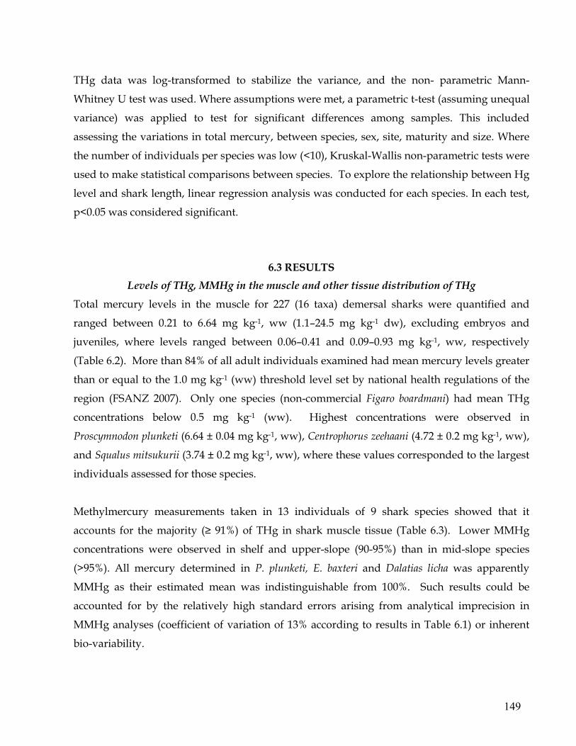
149

THg data was log-transformed to stabilize the variance, and the non- parametric Mann-

Whitney U test was used. Where assumptions were met, a parametric t-test (assuming unequal

variance) was applied to test for significant differences among samples. This included

assessing the variations in total mercury, between species, sex, site, maturity and size. Where

the number of individuals per species was low (<10), Kruskal-Wallis non-parametric tests were

used to make statistical comparisons between species. To explore the relationship between Hg

level and shark length, linear regression analysis was conducted for each species. In each test,

p<0.05 was considered significant.

6.3 RESULTS Levels of THg, MMHg in the muscle and other tissue distribution of THg

Total mercury levels in the muscle for 227 (16 taxa) demersal sharks were quantified and

ranged between 0.21 to 6.64 mg kg-1, ww (1.1–24.5 mg kg-1 dw), excluding embryos and

juveniles, where levels ranged between 0.06–0.41 and 0.09–0.93 mg kg-1, ww, respectively

(Table 6.2). More than 84% of all adult individuals examined had mean mercury levels greater

than or equal to the 1.0 mg kg-1 (ww) threshold level set by national health regulations of the

region (FSANZ 2007). Only one species (non-commercial Figaro boardmani) had mean THg

concentrations below 0.5 mg kg-1 (ww). Highest concentrations were observed in

Proscymnodon plunketi (6.64 ± 0.04 mg kg-1, ww), Centrophorus zeehaani (4.72 ± 0.2 mg kg-1, ww),

and Squalus mitsukurii (3.74 ± 0.2 mg kg-1, ww), where these values corresponded to the largest

individuals assessed for those species.

Methylmercury measurements taken in 13 individuals of 9 shark species showed that it

accounts for the majority (≥ 91%) of THg in shark muscle tissue (Table 6.3). Lower MMHg

concentrations were observed in shelf and upper-slope (90-95%) than in mid-slope species

(>95%). All mercury determined in P. plunketi, E. baxteri and Dalatias licha was apparently

MMHg as their estimated mean was indistinguishable from 100%. Such results could be

accounted for by the relatively high standard errors arising from analytical imprecision in

MMHg analyses (coefficient of variation of 13% according to results in Table 6.1) or inherent

bio-variability.

150

Excluding the single juvenile tested, higher levels of THg were recorded in the muscle tissue (mean 1.49 ± 0.47 mg kg-1, ww), followed by the kidney (0.93 ± 0.14 mg kg-1, ww), liver (0.62 ± 0.25 mg kg-1, ww) and skin (0.12 ± 0.06 mg kg-1, ww), respectively (Table 6.4). Amongst all species, 68 % (range 59–82 %) of the relative total body burden of mercury was stored in the muscle tissue. The kidney accounted for 2.4 % (1–5 %), the liver 9.5 % (1–25 %) and the skin 0.2 % (from below the detection limit to 0.5). For most species, liver, kidney and skin tissue presents statistically lower quantities of mercury than muscle (p<0.01). Unusually large levels of THg were found in the kidneys of Chimaera lignaria (1.62 – 1.97 mg kg-1, ww; 4.8% total body burden) and E. baxteri (0.90 – 4.16 mg kg-1, ww; 4.8% total body burden). Comparably high percentage THg burdens were also found in the livers the two Chimaera species, C. lignaria (0.68 – 1.49 mg kg-1, ww; 12.8 %) and Rhinochimaera pacifica (0.5 mg kg-1, ww; 24.8%). Low levels were observed in the liver and kidney of D. licha (0.7 and 0.9 % relative body burden, respectively) and in the liver of C. zeehaani (2.1 %). Relatively large variability was observed in the majority of tissues tested.

Influence of size and sex on THg of the muscle tissue

In general, THg in the muscle exceeded 1.0 mg kg-1 (ww) above a shark size of approximately 55 cm. On the basis of the ANCOVA, length differences accounted for 85%, 78%, and 71% of the total variation in mercury levels observed in C. zeehaani, Squalus mitsukurii and C. crepidater, respectively. Linear relationships were evident between THg and size for most species, with most regressions being significant with positive slopes, indicating that Hg level increases with increasing length (Fig. 6.1) with lowest values found in embryos and juveniles. R-squared values ranged between 0.43 and 0.98 with more positive correlations observed in C. zeehaani (R2 = 0.98, p<0.001), S. mitsukurii (R2 = 0.88, p<0.001), C. crepidater (R2 = 0.82, p<0.001), and Squalus acanthias (R2 = 0.83, p<0.001) (Table 6.5). Analysis of the THg data by size and sex of shark were tested by ANOVA (where class size was >10 individuals) revealing significant positive correlations for most, but not all species (Table 6.6). Stage of maturity correlated with both the length of male and female individuals, and as such, also significantly influenced THg levels. In most species, females were larger and had higher mean total mercury levels than males, except in Deania calcea, S. mitsukurii and R. pacifica. Sex significantly (ANOVA p<0.05) influenced THg levels in two species; E. baxteri and D. calcea (Table 6.6). However, when THg levels were normalized with size (using BMI; THg mg kg-1/kg bm, ww), higher levels of mercury were in fact observed in males of an equivalent size to females (± 0.5cm).

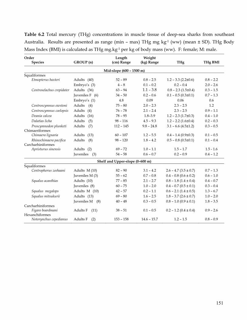
151

Table 6.2 Total mercury (THg) concentrations in muscle tissue of deep-sea sharks from southeast Australia. Results are presented as range (min – max) THg mg kg-1 (ww) (mean ± SD). THg Body Mass Index (BMI) is calculated as THg mg.kg-1 per kg of body mass (ww). F: female; M: male.

Order Species GROUP (n)

Length (cm) Range

Weight (kg) Range THg THg BMI

Mid-slope (600 – 1500 m) Squaliformes

Etmopterus baxteri Adults (40) 52 – 89 0.8 – 2.5 1.2 – 3.3 (2.2±0.6) 0.8 – 2.2 Embryo’s (3) 4 – 8 0.1 – 0.2 0.2 – 0.4 2.0 – 2.6 Centroselachus crepidater Adults (36) 63 – 94 1.1 – 3.8 0.8 – 2.3 (1.5±0.4) 0.3 – 1.5 Juveniles F (6) 34 – 50 0.2 – 0.6 0.1 – 0.5 (0.3±0.1) 0.7 – 1.3 Embryo’s (1) 4.8 0.09 0.06 0.6 Centroscymnus owstoni Adults (4) 75 – 80 2.0 – 2.3 2.3 – 2.5 1.2 Centroscymnus coelopsis Adults (4) 76 – 78 2.1 – 2.4 2.3 – 2.5 0.9 – 1.1 Deania calcea Adults (16) 78 – 95 1.8–3.9 1.2 – 2.3 (1.7±0.3) 0.4 – 1.0 Dalatias licha Adults (5) 98 – 116 4.5 – 9.3 1.2 – 2.2 (1.6±0.4) 0.2 – 0.3 Proscymnodon plunketi Adults (7) 112 – 145 9.8 – 24.8 3.1 – 6.6 (4.5±1.2) 0.3 – 0.5

Chimaeriformes Chimaera lignaria Adults (13) 60 – 107 1.2 – 5.5 0.4 – 1.4 (0.9±0.3) 0.1 – 0.5 Rhinochimaera pacifica Adults (8) 98 – 120 1.8 – 4.2 0.5 – 0.8 (0.5±0.1) 0.1 – 0.4

Carcharhiniformes Apristurus sinensis Adults (2) 69 – 72 1.0 – 1.1 1.5 – 1.7 1.5 - 1.6 Juveniles (3) 54 – 58 0.6 – 0.7 0.2 – 0.9 0.4 – 1.2

Shelf and Upper-slope (0–600 m) Squaliformes

Centrophorus zeehaani Adults M (10) 82 – 90 3.1 – 4.2 2.6 – 4.7 (3.5 ± 0.7) 0.7 – 1.3 Juveniles M (3) 55 – 62 0.7 – 0.8 0.4 – 0.8 (0.6 ± 0.2) 0.6 – 1.0 Squalus acanthias Adults (10) 77 – 85 2.1 – 2.7 0.8 – 1.8 (1.4 ± 0.4) 0.4 – 0.7 Juveniles (8) 60 – 75 1.0 – 2.0 0.4 – 0.7 (0.5 ± 0.1) 0.3 – 0.4 Squalus megalops Adults M (10) 42 – 57 0.2 – 1.1 0.6 – 2.1 (1.4 ± 0.5) 1.3 – 6.7 Squalus mitsukurii Adults (13) 69 – 80 1.6 – 2.5 1.8 – 3.7 (2.6 ± 0.7) 1.0 – 2.0 Juveniles M (8) 40 – 48 0.3 – 0.5 0.8 – 1.0 (0.9 ± 0.1) 1.8 – 3.5

Carcharhiniformes Figaro boardmani Adults F (11) 38 – 51 0.1 – 0.5 0.2 – 1.2 (0.4 ± 0.4) 0.9 – 2.6

Hexanchiformes Notorynchus cepedianus Adults F (2) 153 – 158 14.6 – 15.7 1.2 – 1.5 0.8 – 0.9

152

Table 6.3 Percentage (%) of MMHg (mg kg-1 dw) that accounts for THg (mg kg-1 dw). Values are taken as the mean from 1–4 replicates were performed on each individual. n: number of determination.

Habitat Species (n)

Sex

THg

MMHg

MMHg/THg (%)

Mid-slope C. crepidater (2)

F

7.5 – 8.0

7.1 – 7.8

94.6 – 97.5

C. owstoni F 10.0 9.6 95.8 D. licha M 8.4 8.5 101.3 E. baxteri F 10.8 11.0 101.1 P. plunketi (2) M 17.5 – 20.6 17.1 – 21.3 97.5 – 103.4 Shelf and Upper-slope S. acanthias

F

6.0

5.6

93.3

S. megalops F 6.9 6.3 91.3 S. mitsukurii F 10.5 9.9 94.3

Table 6.4 Range (min – max) of total mercury concentrations (mg kg-1, ww) in the tissues of ten species of shark from south eastern Australia. Muscle Liver Kidney Skin ww Conversion factor: 22-26 7-9 15-16 16-19

Species (n) Length (cm) Total mercury (THg) C. crepidater (3) 80–88 1.05 – 1.60 0.24 – 0.46 0.67 – 0.81 0.11 – 0.28 C. crepidater pup (1) 34.6 0.12 0.02 0.05 0.00 C. lignaria (2) 106–111 0.86 – 1.15 0.68 – 1.49 1.62 – 1.97 0.11 - 0.26 C. zeehaani (1) 82.5 2.47 0.18 1.05 0.02 D. licha (1) 98.8 1.06 0.49 0.27 0.13 E. baxteri (4) 56–98 1.55 – 2.86 0.47 – 1.3 0.90 – 4.16 0.10 – 0.19 P. plunketi (3) 112–126 2.69 – 4.50 0.84 – 1.34 1.67 – 1.84 0.17 – 0.24 R. pacifica (1) 112 0.4 0.5 0.17 0.08 S. acanthias (2) 75–82 0.64 – 1.45 0.61 – 0.83 – 0.12 – 0.18 S. megalops (2) 44–48 0.75 – 0.79 0.38 – 0.70 0.28 0.03 – 0.1 S. mitsukurii (2) 75–79 2.83 – 3.23 – 1.35 – 1.63 0.14

Average 50.3 22.4 27.4 4.4 Relative tissue burden (%) Range 26.2 – 66.4 4.9 – 42.3 13.7 – 47.7 0.5 – 6.9

Proportion tissue of whole weight (%) 45 – 65 6 - 30 1 - 4 1.9 Average 68.1 9.5 2.4 0.2 Relative total body

burden (%) Range 59.1 – 81.8 1.0 – 24.8 0.9 – 4.8 0.0 – 0.5

* Proportion tissue burden (%) is the tissue-to-total body ratio for each specified tissue, and is taken from published (muscle: Daley et al. 2002b) and unpublished data. Wet weight (ww) conversion factor is the % of total water content and was used to convert dry mass concentrations to wet mass. Relative tissue burden is calculated as the proportion of mercury (mg kg-1, ww) within a certain tissue relative to all other tissues tested. Relative body burden is calculated as percent (%) THg in a tissue relative to the tissues contribution to the whole body weight. n: number of determination.

153

Table 6.5 Regression analysis of Log (THg) level as a function of size for demersal sharks species. Significant linear functions (Y= a + bx) were fitted. Y = Log (THg) level (mg kg-1 ww), x is total length (cm). The estimated intercept (a), slope (b), R2 value and P value are listed by species. Equations based on all data, regardless of location and time of collection, except where outliers were present in the data set. n: number of determinations.

Species (n) a b R2 P-value

C. crepidater (42) 1.10 0.015 0.82 >0.001 C. lignaria (14) 0.67 0.007 0.68 0.012 C. zeehaani (13) 1.92 0.029 0.98 >0.001 E. baxteri (40) 0.27 0.009 0.43 0.010 D. calcea (19) -0.27 0.005 0.24 0.075 S. mitsukurii (21) 0.64 0.061 0.88 >0.001 S. acanthias (18) 2.29 0.054 0.83 >0.001 S. megalops (15) -0.61 0.009 0.06 0.171 F. boardmani (11) 2.36 0.065 0.78 >0.001

Geographical, vertical distribution and inter-specific variations

Mercury concentration varied between species and taxon (Table 6.1) according to biology and

environment (Table 6.6). No significant relationships between collection site and THg was

observed for C. crepidater collected in the east and south off Tasmania, nor for sharks of

different species collected in the Great Australian Bight and Tasmania. In contrast, some

variation in THg concentrations was explained by habitat type, where species were separated

by their vertical distribution (shelf and upper-slope vs mid-slope, Table 6.6). In general, higher

mean concentrations of Hg in sharks appeared in deep-demersal species, although these were

not seen to be highly significantly different (p = 0.058). To take away the effects of biological

variation (including some effects of size and physiology), species from the Order Squaliformes

were pooled together for comparisons of habitat and THg. Squalids occupying the shelf and

upper-slope had higher mercury levels relative to their size (BMI) than mid-slope species (0.6 –

2.5 and 0.3 – 1.5 THg/kg bm, respectively). The exception was the mid-slope southern lantern

sharks, E. baxteri which showed mean concentration levels of 1.41 THg/kg bm and were

statistically higher than those of other mid-slope squalids (p=0.01). In comparison to other

taxon groups, the two Scyliorhid species, deepwater catsharks F. boardmani and A. sinensis,

contained higher BMI levels than the averages of those Squalids occupying similar water

154

bodies. The upper-slope Hexanchid species, Notorynchus cepedianus showed the lowest

mercury levels relative to BMI (0.08 – 0.1 THg/kg). Regardless of slope habitat, all juveniles

displayed similar THg levels (BMI, 0.5 – 0.9 THg/kg). Inter-annual and inter-seasonal

variation in Hg level was investigated and all taxa examined showed no effect for either factor

(Table 6.6). For many species, sample size limitations did not warrant inter-annual and/or

regional comparisons.

-1.0

-0.8

-0.6

-0.4

-0.2

0.0

0.2

0.4

0.6

0.8

30 40 50 60 70 80 90 100

Total length (cm)

Log

(TH

mg

kg -1

ww

)

Figure 6.1 Log10(THg) concentration of shark muscle vs total length (cm) for four shark species: ■ Centroselachus crepidater, ○ Etmopterus baxteri, ∆ Squalus acanthias, ▲ Squalus mitsukurii

155

Table 6.6 Probability values for species-specific ANOVA results examining sex, year, season and location effect on THg levels. *P < 0.05, N/A: insufficient data for statistical treatment. Mid-slope species consist of E. baxteri, C. crepidater and D. calcea; Upper-slope species consists of S. acanthias and S. mitsukurii. P-value

Species / group Sex M vs. F

Year 2005 vs. 06

Season S vs. W

Location Tas vs. Vic

Maturity 1,2 vs. >3

BMI (THg/kg) vs. Sex

E. granulosus 0.031* 0.326 0.356 N/A 0.012 * 0.01 * C. crepidater 0.111 N/A 0.274 0.253 0.009 * 0.015 * D. calcea 0.040* N/A N/A N/A 0.023 * 0.053 S. mitsukurii 0.093 N/A N/A N/A 0.032 * 0.022 * Mid- vs Upper-slope 0.127 N/A 0.124 0.058 0.072 0.032 * All species 0.346 0.427 0.267 N/A 0.041 * 0.029 *

6.4 DISCUSSION

The present study brings new results on the mercury levels in several species of demersal

sharks from the Australian waters, in relation to their development stage, size, sex and habitat.

In addition, it provides comment on the food safety implications of human consumption of the

flesh of these animals.

Mercury and shark life-cycle

Basic information about the mercury pathway and dynamics within the shark may be

extracted from the results on Hg tissue distributions (organotropism) and growth-related Hg

variation (embryos, juveniles, size and sex Hg dependences).

Organotropism - In some marine organisms, methylmercury tissue concentrations are related to

the uptake rate (gill, intestine), others to the demethylation and excretion rate (liver, kidney)

(Boening 2000). In sharks, like most high-order marine predators, dietary mercury is

incorporated in a dose-dependant manner (Boudou & Ribeyre, 1997), and is accumulated in

internal tissues. Few studies have tested the partitioning of mercury in demersal

chondrichthyes. Hornung et al. (1993) reported THg content in various tissues of five

deepwater species (including Centrophorus granulosus, Galeus melastomus and Etmopterus spinax)

156

from the eastern Mediterranean Sea. In all species, they found that higher levels of Hg were

observed in the kidney and ‘healthy’ livers than in the muscle tissue, with highest (up to 11

times greater in C. granulosus) concentration being observed in unhealthy (very dark) livers.

Similarly, in pelagic sharks, Boush and Thieleke (1983) showed that in sexed sharks

(Garcharhinus limbatus), significantly higher levels were observed in the liver (0–5.5 mg kg-1)

than the muscle tissue (0–2 mg kg-1), although the opposite was true for the tiger shark

(Galeocerdo cuvieri, n=13), which displayed higher THg levels in the muscle tissue (0.1–0.65 mg

kg-1) than the liver (0–0.25 mg kg-1), possibly illustrating different physiological capacities to

process Hg between these species.

In this study, the highest mercury concentrations and more than half the total mercury burden

were found in the muscle tissue. The kidney showed relatively high THg levels along with the

liver, and minute amounts were found in the denticles (skin). This suggests that mercury is

taken up through the diet rather than the environment, and is readily dispersed throughout

the body and cumulatively stored in muscle tissue. In contrast, the digestive tissues (kidney

and liver) are likely to be associated with metal metabolism, storage and elimination

procedures. In species (and individuals) that have relativity higher Hg concentrations in the

kidney (Chimaera lignaria and E. baxteri) and liver (R. pacifica and C. lignaria) than other species,

it might suggest either recent exposure followed by concentration in the liver, or strong protein

binding, perhaps in a similar manner as has been demonstrated with cadmium by Lucis et al.

(1970). Multiple factors are likely to have contributed to the higher individual variability and

different trends in the tissue distribution of mercury observed in demersal sharks by Hornung

et al. (1993) than in this study. Firstly, although similarities within genera can be drawn, inter-

species variability in metabolism and physiology are likely to be large. Secondly, sharks

studied by Horung et al. (1993) were collected near a deepwater dumpsite, and thus, were

atypical (affected by variable and elevated Hg concentrations from localised pollution).

Influence of size and sex - The linear relationships observed in almost all species demonstrates

that larger, presumably older individuals accumulated higher levels of mercury. This pattern

has been extensively exhibited in previous studies of sharks (Forrester et al., 1972; Walker,

1976, 1988; Taguchi et al., 1979; Hueter et al., 1995). For C. crepidater analysed in this study,

157

comparable Hg levels and a similar relationship between size and Hg levels have been

observed (Davenport 1995; Turoczy et al. 2000). The accumulation of mercury with increasing

size (fundamentally age) is likely to also reflect other ecological and physical factors, such as

differential feeding ecology, and slow and inefficient elimination of mercury from deeper

dwelling species (Trudel & Rasmussen 1997). It is widely recognized that diet is the most

important source of Hg exposure in marine top predators (Boening 2000). Thus, it can be

assumed that the wide range of mercury concentrations observed in this study were a

consequence of distinct feeding habits, in addition to other species-specific parameters, such as

metabolism and growth rates. Furthermore, data presented here suggest that through

bioaccumulation, larger, older adults of these common species potentially contain excessive

mercury burdens. Where variability was high in adult individuals, stage of maturity was

positively correlated with increasing mercury levels. Ontogenetic variations in diet may also

be a considerable factor, particularly where differences are observed between juveniles and

adults. In contrast to length, similar THg levels were not often correlated with body weight.

This indicates that there is a change in the proportion between size and weight to a certain

degree, especially as the shark's shape changes in relation to storage of energy and/or sexual

maturity. Although aging, therefore, would have been better than weighing, information on

the growth rates of demersal sharks is limited, Aging studies (from spines) of dogfish sharks

around Tasmania (Irvine et al., 2006) suggest that our specimens ranged between 15 and 48

years, excluding juveniles. Relationships between aging estimations and size of sharks are

thought to be quite variable, possibly explaining some of the observed variability of mercury

levels in sharks, particularly where juvenile and sub-adult specimens were also tested.

As a group, females in most species showed higher values than males; however, males that

were of a similar length gave higher mean mercury levels. Such phenomena have been

observed in S. mitsukurii (Taguchi et al. 1979), and in Squalus megalops (De Pinho et al. 2002).

Similar to most elasmobranchs, female demersal sharks have higher growth rates and are

larger (sometimes up to 40%) than males (Daley et al. 2002b), displaying sexual dimorphism.

This indicates that although males are smaller, they may be of a similar or older age group to

larger females. Several species tested in this study have complex population structures,

exhibiting segregation by sex, size and mature condition (Daley et al. 2002a; Last & Stevens

158

2009). Differences in mercury levels in males and females may be caused by factors such as

energetic requirements, maturation condition, mercury deposition, and transference to eggs

and fetuses (Walker 1976). In sharks that are characterized by viviparous reproduction, due to

the transfer of mercury to the fetus, females of some sharks may have lower concentrations of

mercury than males; however this was not shown to be the case in this study.

Maternal transfer to embryos and juveniles - Because mercury levels increase as individuals grow

larger, observed levels in embryos and juveniles can be viewed as the base concentration for

the overall population, and indicate the transfer of mercury from maternal sources. Total

mercury levels in embryos ranged from 4-10% of levels observed in their mothers, whose

mercury levels were greater than 1.5 mg kg-1. Marginally higher Hg levels were observed in E.

baxteri than the sympatric squalid C. crepidater, although they are both viviparous and have

similar estimated gestation periods (Last & Stevens, 2009). Walker (1976) suggested that

transfer of mercury to developing ova and embryos may reduce mercury levels in mature

females. In the present study, such relationships were not clearly shown with relatively

similar mercury levels recorded in pregnant and non-pregnant females, despite the effects of

maternal transfer of mercury to developing ova and embryos. Increased dietary needs, and

thus, an increased uptake of MMHg, may be responsible for these similarities.

Adams and McMichael (1990) studied mercury levels in embryos, neonates and juveniles of

three Carcharhinid and one Sphyrnid sharks, which have placental viviparous reproduction.

All species showed greater mean mercury levels (embryos 0.16–0.78, juveniles 0.17–1.7) than

those reported in this study for both E. baxteri (embryos, 0.2–0.4 mg kg-1, no juvenile data) and

C. crepidater (embryo 0.06 mg kg-1, juveniles 0.1–0.5 mg kg-1). The reproduction mode,

combined with other physiological factors associated with family and habitat differences,

conceivably explain why aplacental viviparous shark embryos contained the lowest mean

mercury levels in this study. Squalids are viviparous, where nutrients are derived from an

associated yolk sac; and thus, high concentrations would possibly be expected due to the direct

interchange of nutrients (and presumable mercury) between the mother and embryo via the

placenta. Jeffree et al. (2008) showed that that the egg case of dogfish (Scyliorhinus canicula) is

highly permeable to chemotoxic metals such as Hg and that there is much capacity for

159

developing embryos to accumulate very high concentrations of Hg, such as was displayed in

this study. In most viviparous sharks, developing oocytes take up large amounts of maternally

derived vitellogenin, which consist of about 30% lipid (Chapter 3) and thus lipid metabolism

may play a role in transgenerational contaminant transfer (Landrum & Fisher 1998). This

pathway would be particularly important for well-known lipophilic contaminants, such as

DDT and PCBs but is unlikely to be as important for MMHg which preferentially forms bonds

with thiol-containing molecules, such as proteins and amino acids (Bloom 1992). In this

regard, it seems vitellogenin (Vtg), a lipophosphoprotein yolk-granule precursor produced in

the liver and taken up by developing oocytes (Hamlett & Koob 1999) may have the ideal

characteristics in which to transport MMHg to embryos by tightly bounding to sulfhydryl and

other sulfur functional groups associated with these proteins.

In juveniles, variable mercury concentrations were found (Table 6.4). For juveniles of S.

acanthias, much lower Hg levels were found in larger specimens collected in the Celtic Sea

(Domi et al. 2005) than were reported in smaller specimens in this study. Greig et al. (1977),

found low Hg concentrations in the fetuses of S. acanthias, and concluded that in this species

mercury does not transfer from the mother to the fetus. Such a conclusion suggests that the

higher Hg levels recorded in the juveniles of S. acanthias in this study, compared with Domi et

al. (2005), were accumulated after hatching and may be an effect of regional differences in diet.

Interspecific, local and regional Hg variations in sharks muscle tissue

Information regarding mercury in demersal sharks around the world is scarce. For

comparisons with this study, only for the genera Centrophorus, Etmopterus, Squalus, Dalatias,

Deania and Chimaera are some published data available (eg. De Pinho et al. 1989; Hornung et al.

1993 ; Davenport 1995; Turoczy et al. 2000; Storelli et al. 2002; and reviewed by Cossa &

Coquery, 2005). Results from the present study are the first published for dogfish, Etmopterus

baxteri, Proscymnodon plunketi, chimaeras, Rhinochimaera pacifica, and Chimaera lignaria, and

deepwater catshark, A. sinensis and Figaro boardmani. WE contend that mercury concentration

in the shark muscle tissue, in addition to size and sex dependence (see subsequent sections), is

related to the species and their habitats.

160

Mercury levels varied greatly amongst species, although noticeably all specimens from the

Order Squaliformes had the highest levels of mercury recorded, and mean mercury levels

strongly exceeding the 1.0 mg kg-1 (ww) threshold. In comparison, the families Scyliorhidae,

Chimaeridae and Rhinochaeridae had relatively lower mean mercury levels (<1.0 THg mg kg-1,

ww). This is not surprising as these families share lower trophic levels (Cortés 1999), and

highlights that Hg uptake is strongly related to diet (Domi et al. 2005). However, the sevengill

shark, N. cepedianus (Hexanchidae) had the lowest body mass index (BMI = 0.09) of any

species, indicating low accumulative levels despite its known diet of high trophic status

(Cortés 1999). Such results emphasize that multiple factors are important in the accumulation

of mercury in sharks, including environment, physiology and ecological interactions.

Results of several studies around southeastern Australia (Walker 1988; Davenport 1995;

Turoczy et al. 2000) show similar mean mercury levels in the muscle tissue to those reported in

this study. Comparable elevated levels are also documented in several demersal sharks,

globally (De Pinho et al. 2002; Storelli et al. 2002). However, when comparing these results

with those of our study, taxon and regional differences in Hg biomagnification do seem

present. For example, Storelli et al. (2002) reported higher concentrations in similar sized

specimens of the kitefin shark, D. licha collected from the Ionian Sea (Eastern Mediterranean

Sea) than in those of this study. Similarly, in the Portuguese dogfish C. coelolepis, lower

concentrations in the muscle were reported in specimens collected off south-eastern Australia

(Davenport 1995 and this study) than those of a similar size range collected from the

Mediterranean (Cossa & Coquery, 2005). This is also true for deepwater catshark species, for

which higher concentrations have been observed in the Mediterranean (Horung et al. 1993),

than in those presented in this study for Figaro boardmani (previously known as Galeus

boardmani), while comparable levels have been reported in the Celtic Sea (Domi et al. 2005).

Storelli and Marcotrigiano (2002) found that for similar sized specimens of blackmouth

dogfish, Galeus melastomus, THg and MMHg concentrations differed substantially among those

collected from the Adriatic Sea, the Ionian Sea and the Aegean Sea, demonstrating the strong

affect that the environment has on mercury uptake. In D. calcea, similar levels were recorded

in similar sized species collected from waters of the Mid-Atlantic Ridge (Martins et al. 2006) to

those collected off south-east Australia (Davenport 1995; Turoczy et al. 2000 and this study). In

161

a first attempt, it can be suggested that margin waters from open oceanic environments such as

the Australian and Celtic shelves, harbour sharks with lower mercury content than those from

an epicontinental environment, such as the various basins of the Mediterranean Sea. However,

this generalization is not yet supported by available environmental data. We also have to

consider that food chain structure or growth rate differences between Mediterranean sharks

and those from other oceanic regions might equally explain these observations. Indeed, the

range of MMHg concentrations measured very recently in the water column of the

Mediterranean Sea (Cossa et al. 2009), Tasmanian margin (Cossa et al. 2008) and Celtic Sea

(Cossa & Chou, unpublished) are similar (<0.01–0.15 ng L-1). Further studies of mercury

cycling in the Mediterranean Sea, and the dynamics of the heavy metal in the region’s food

chains topped by demersal sharks, are required to establish the basis for their greater mercury

burden in these waters.

At a smaller geographical scale (East and South Tasmania vs Victoria), the habitat effect on

mercury concentration in sharks seems less clear. Differences between shelf/upper-slope

species and mid-slope species are noted in our study, although differences between collections

sites were not detected for the majority of taxa examined. A lack of variability between taxa

and site are likely to indicate similar associations among predatory behavior, longevity, and

mercury accumulation processes as has been suggested by Forrester et al. (1972). Furthermore,

similarities in diet and base-level mercury concentrations, hydrodynamic patterns, and the

movement of the migratory species are additional factors likely to exclude within regional

differences in Hg biomagnification in the sharks reported in this study.

Deep-sea environments are considered to be the sink and final reservoir for contaminants

(Tatsukawa & Tanabe 1984). Deep-sea species are long-lived, and tend to feed at higher

trophic levels than their shallow-water counterparts Hence, they are exposed to higher levels

of recycled elements for longer periods (Gordon et al. 1995), and the corresponding

accumulation of most trace metals is likely to be greater. In this study, higher concentrations

appeared in deep-demersal species which may be related to the consumption of prey from

different food chains. Sarica et al. (2005) found that marine predators with scavenging

behavior have a greater potential to assimilate methylmercury. This seems true in regards to

162

the high levels found in the demersal sharks reported in this study. Alternatively, differences

between shelf/upper-slope species and mid-slope species may also be attributed to differences

in lipid biochemistry and increasing lipid content in the liver with depth (Chapter 2) which

may affect the ability of the liver to demethylate mercury.

The absence of any long-term, seasonal or annual differences (summer, winter and 2005, 2006)

for the majority of the taxa examined is consistent with the fact that all samples were

considered of adult size, and presumably older than 20 years. In a 20-year accumulation time,

a one-year sampling difference is a relatively short time interval in which natural or

anthropological events could cause environmental changes. Additionally, sharks, being high-

order predators with slow metabolisms, accumulate mercury over longer time periods than

those occupying the lower trophic levels, leading to greater biomagnification of mercury. For

example, Sager (2002) found elevated Hg levels in predatory fishes 30 years after a local Hg-

contaminated water release was ended even though the Hg level of some fishes at lower

trophic levels dropped below the safety level the next year.

Conclusions

Regardless of species, in all adults, mercury concentrations of the muscle tissue are high

enough to cause potential health concerns for sustained and regular human consumption

(Harada 1995) and are over the local (FSANZ 2007) and European Union legal limit (EFSA

2008) for mercury in fish of 1.0 and 0.5 mg kg-1 (ww), respectively. MMHg is the most toxic

form of mercury for human consumption, and essentially accounts for the majority (>90%) of

mercury found in fish muscle tissue (eg. Bloom, 1992), as well as in the sharks studied here. In

other studies on sharks (Walker 1976; Storelli et al. 2002), methylmercury has been recorded to

represent between 50–100% (most exceeding 70%) of the total mercury content in muscle

tissue.

This study has provided information on the contamination status of mercury in demersal

chondrichthyes, which are less studied than teleost fish. The longevity and slow growth rates

of demersal sharks, considered in conjunction with their apex predator life-style contribute

significantly to the accumulation of high concentrations of mercury that warrant public

163

concern as many species reported here are still being fished and marketed. The variations of

mercury concentrations among species are likely to be most affected by the trophic level at

which they feed and physiological differences in metal assimilation and metabolic capacity in

processing MMHg. Large-scale regional differences in Hg levels seem apparent in

chondrichthyes, which emphasis the important position of the environment and ecology in

mercury biomagnification and also stimulate consideration of these high-order predators as

environmental monitors. Further research, with increased and targeted sample sizes of certain

ubiquitous species, size ranges, and locations would help elucidate the relationship of MMHg

to the specific migratory habits and physiology of demersal sharks.

164

7

TROPHIC STRUCTURE AND BIOMAGNIFICATION OF MERCURY IN DEEPWATER CHONDRICHTHYANS COLLECTED OFF SOUTH-

EASTERN AUSTRALIA

165

CHAPTER 7

TROPHIC STRUCTURE AND BIOMAGNIFICATION OF MERCURY IN

DEEPWATER CHONDRICHTHYANS COLLECTED OFF SOUTH-EASTERN AUSTRALIA

ABSTRACT Deepwater chondrichthyans play a key role in marine ecosystems, but knowledge of their feeding habits and contaminant bioaccumulation is limited. In this study, stable isotope ratios of carbon (δ13C) and nitrogen (δ15N) were used to evaluate predator-prey interactions, community structure and to assess trophic pathways and mechanisms that influence mercury accumulation in 16 deepwater chondrichthyan species (primarily, Centroselachus crepidater and Etmopterus baxteri) from south-eastern Australia, through 2004–2006. In all species, δ15N ranged from 12.4 to 16.6 ‰ and a broad range of trophic positions were calculated (3.6 – 4.7) from analyses of the muscle tissues. Minor variation in δ13C enrichment was observed between species (–18.7 to –17.1‰) with the exception of Squalus acanthias (–19.3 ± 0.1‰) reflecting a pelagic foraging strategy. Total mercury (THg) levels in shark muscle ranged from 0.3 to 4.5 mg kg-1 (wet weight, ww) with the highest concentrations coming from the two largest individuals of Proscymnodon plunketi. In individual shark species, mercury concentrations increased with size and trophic position, whereas associations with carbon source were only present in C. crepidater. As a community, deepwater elasmobranchs demonstrated moderate rates of THg biomagnification, as indicated by the regression slope (log (THg) = 0.18 δ15N – 2.25, R2 = 0·33, P < 0·05). Comparisons between taxa and habitat illustrated that food-web structure, environmental and physiological traits play an important role in the mercury biomagnification in deepwater chondrichthyans.

166

7.1 INTRODUCTION Knowledge of trophic ecology, which includes feeding relationships among organisms in an

ecosystem, is paramount in understanding food web structure, in addition to the function and

movement of chemicals through it. Natural stable isotopes of carbon and nitrogen are

increasingly being used in a variety of marine biota to explore quantitatively the trophic-

dynamics and energy flows in food webs (Peterson & Fry 1987), time-integrated food-web

structure (Post 2002), habitat usage (Hobson 1999) and migration (Hansson et al. 1997). Changes

in isotope ratios (i.e. fractionation) occur through metabolic processes, which, in general, cause

the lighter isotope to be preferentially lost and the heavier one to be retained. Carbon isotope

ratios (δ13C) remain relatively unaffected by trophic transfer (Fry & Sherr 1984), being typically

enriched by ~1‰ per trophic position (Peterson & Fry 1987, Hobson & Welch 1992) and can be

used to indicate different potential primary sources in a trophic web, such as aquatic vs.

terrestrial, nearshore vs. offshore, or pelagic vs. benthic contributions to food intake (Hobson et

al. 1995). Stable nitrogen isotope ratios (δ15N) show a systematic mean enrichment of around

3.4‰ with each increasing trophic level (Minagawa & Wada 1984); from these, relative trophic

positions can be estimated (Post 2002).

Sharks species range from trophic levels of 3.1 to 4.5 (Zebra shark to great white shark), with

the majority in excess of four (Cortés 1999), similar to those of marine mammals (Lesage et al.

2001) and higher than those of seabirds (Hobson et al. 1994). To date, eight studies (eg. Rau et

al. 1983; Davenport & Bax 2002; Estrada et al. 2003) on just 13 species of sharks have used

stable isotope analyses to estimate trophic level. Of these, only four occurred in waters deeper

than 200 m, including Somniosus microcephalus (Fisk et al. 2002), Squalus acanthias, Galeus

melastomus and Scyliorhinus canicula (Domi et al. 2005).

Increasingly, stable isotopes have also been coupled with contaminant analysis to delineate

patterns and extent of biomagnification in marine food webs (Hobson & Welch 1992; Atwell et

al. 1998; Power et al. 2002). In particular, the consistency of δ15N enrichment at each trophic

transfer provides a convenient quantitative measure of relative trophic position within a food

web (Cabana & Rasmussen 1994; Post 2002). It may be correlated with contaminant

concentrations to estimate metal uptake and biomagnification rates (eg. Power et al. 2002).

167

Currently, only two studies have looked at the relations of metal biomagnification in

elasmobranch species (Domi et al. 2005, Fisk et al. 2002). Domi et al. (2005) demonstrated that

both cadmium and mercury were correlated with isotopic ratios δ13C and δ15N, and this was

shown to be diet-related in the spiny dogfish Squalus acanthias and the black-mouthed catshark

Galeus melastomus.

Mercury (Hg) is an environmental contaminant present in marine systems globally and the

health implications of methlymercury (MeHg), especially neurologically, on both animal and

human health are well reported (reviewed by Eisler 2006). One of the major concerns is the

potential for it to biomagnify, as it moves up food webs, resulting in more harmful

concentrations in top-level predators, particularly if they are large and long-lived. In aquatic

organisms, the uptake and accumulation of MeHg is influenced by complex biological,

ecological and environmental factors (Boudou & Ribeyre 1997, Chen et al. 2008), with dietary

uptake, age and size key variables (Hall et al. 1997; Cabana & Rasmussen 1994; Wiener et al.

2003). Species-specific physiology and metabolism have also been viewed as important

variables (Fisk et al. 2002). Understanding the mechanisms of contaminant bioaccumulation in

food webs is critical to predicting which pathways are at risk of both higher rates of

bioaccumulation and greater concentrations of biomagnification, which in turn may endanger

the health of apex-predators, including humans.

Mercury concentrates in the marine environment, particularly in deep ocean waters (Mason

and Sheu 2002). In general, deep-sea species are longer lived, have slower growth rates

(Gordon et al. 1995) and may feed at higher trophic levels than species from continental shelf

areas (Cronin et al. 1998), thus being exposed to higher levels of contaminants (Gordon et al.

1995). In contrast to the wealth of knowledge on trace element concentrations in near shore

and pelagic organisms (eg. Campbell et al. 2005), very little is known about metal

accumulation in deep-sea and bathypelagic organisms (Cronin et al. 1998; McArthur et al.

2003). Likewise, despite their predatory dominance and their important contribution to the

structure and function of ecosystems, very few studies have quantitatively assessed the trophic

ecology of demersal chondrichthyans. Here, we investigate the trophic relations and patterns

of Hg biomagnification in several demersal shark and chimaera species. The purpose of this

168

study was to use carbon and nitrogen signature isotopes to examine the trophic status and

accumulation pathways of Hg in a community of deepwater chondrichthyans abundant off

continental shelves that support a number of commercial fisheries. Regression models were

used to estimate trophic position, Hg biomagnification and uptake, to elucidate Hg

accumulation dynamics and to consider relative Hg exposure routes.

7.2 MATERIALS AND METHODS

A total of 67 individual sharks of 16 species were collected from continental shelf and slope

waters (>200 m) around eastern and southern Tasmania, and south west off Victoria, between

2004 and 2006 (Fig. 7.1). Most samples were taken on an opportunistic basis as by-catch from a

local commercial fishing trawl, the Adriatic Pearl, while targeting orange roughy (Hoplostethus

atlanticus). Other samples were taken onboard the Cape Hood, Dianna, Saxon Onwards, Saxon

Progress and other commercial fishing boats while targeting predominantly ling, demersal

sharks and blue grenadier. All shark species were identified, individually weighed and

measured. Species names are taken from the most recent literature (Last & Stevens 2009). Two

subsamples of 100 g of muscle tissue (obtained posterior to the dorsal fin) were collected in

polyethylene zip-lock bags and stored at -20 ºC. All homogenous tissue samples were freeze

dried (–80ºC for up to 60 h) and ground to fine powder (mesh size 100-200 µm) with a mortar

and pestle.

Approximately 1.0 mg of dried, ground muscle tissue was used in the simultaneous analysis

for carbon, nitrogen, isotopic carbon (δ13C) and nitrogen (δ15N). The instrument used a coupled

elemental analyser with an isotope-ratio mass spectrometer (EA-IRMS) at Griffith University,

Australia. Stable isotope ratios are expressed as delta values (δ13C, δ15N) and measured as

parts per thousand differences (‰) relative to ANU Sucrose and atmospheric N (Air) for

isotopes δ13C and, δ15N, respectively. Replicated measurements of internal laboratory

standards (Acetanilidae) and working standard (prawns) gave precision errors of ± 0.1 and ±

0.2 ‰ for δ15N and δ13C, respectively. Trophic Position (TP) of shark species was estimated

from δ15N values following the equation:

TP = (δ15Nshark - δ15Nphyto)/ 3.4 + 1 (after Cabana & Rasmussen 1994).

169

δ15Nshark is the trophic level of the shark species, indicative by its nitrogen isotopic ratio,

δ15Nphyto nitrogen isotopic ratio of marine phytoplankton and particulate organic matter (POM,

4.1 based on that in oceanic water off southeast Australia, Davenport & Bax 2002), and 3.4 (‰)

taken as the mean nitrogen fractionation between two trophic levels (Minawaga & Wada 1984;

and reviewed by Post 2002).

Figure 7.1 Map of collection area, Australia and Tasmania

Total mercury (THg) analyses were undertaken in company of a larger data subset reported in

Chapter 6. In brief, analyses of total mercury (THg) were carried out on two to three replicate

samples ranging from 10–50 mg of dried muscle tissue. THg concentrations were determined

by flameless atomic absorption spectrometry using an Advanced Mercury Analyser AMA 254

(Altec, Prague, Czech Republic). Greater detail of the methodology is reported in Cossa et al.

(2002). The accuracy and the reproducibility of the method were established using an

international certified standard (DORM-2, National Research Council Canada). The certified

values were reproduced within confidence limits up to 95%. Precision was further determined

by analysing blanks and replicate samples. The detection limit and the reproducibility are

0.007 ng.mg-1 per dry weight (dw) and 7 %, respectively. THg concentrations are reported in

170

mg kg-1, as total Hg per wet weight (ww). Total water content of the muscle tissue was used to

assess the dry weight to wet weight ratio. Speciation analysis of mercury (reported in Chapter

6) demonstrated that 91% of THg was present as methylmercury (MeHg) in the white muscle

tissue of most documented shark species; and thus, THg was deemed an appropriate

representative of the more toxic MeHg.

The ability of a contaminant to biomagnify can be expressed in terms of trophic

biomagnification factors based on the trophic position parameter (such as those inferred by

δ15N) in a linear regression model. Such factors have been applied to a number of whole

ecosystem studies (eg. Atwell et al. 1998; Campbell et al. 2005) and separately for a group of

high-order predators (eg. fish: Power et al. 2002; seabirds: Hop et al. 2002). It is derived from

the slope of the log-linear relation between contaminant concentrations and trophic position as

given by the equation:

Log (Hg) = a + b TP + e.

Where a is the intercept, b is the slope and e is the error estimate.

Due to limited sample replication for each species, statistical analyses were only performed on

two shark species (Etmopterus baxteri and Centroselachus crepidater) which had sample sizes

greater than 20. To assess community relations, species were pooled together for statistical

analyses. Pearson linear regressions were used to examine correlations between shark

characteristics (eg. length and habitat), THg and isotope data (δ15N, δ13C). Differences in slope

and elevation, along with group differences within the dataset were tested using ANCOVA

and post-hoc multiple comparison (Tukey) test’s. Where multiple regression models were

undertaken, mercury concentrations were log-transformed for comparisons with other studies

on biomagnification rates. Analysis of variance (F-test) was used to establish the significance of

additional model variables, and standardized regression coefficients were used to infer the

relative importance of each independent variable for explaining variations in the dependent

variable. A p-value of less than 0.05 was considered to indicate statistical significance. All the

statistic analyses were performed using SPSS software (SPSS Inc. Chicago, Illanois).

171

7.3 RESULTS Carbon and nitrogen isotopes

Carbon and nitrogen stable isotopes (δ13C, δ15N) and C:N ratio for all 16 species of demersal

chondrichthyans are presented in Table 7.1 along with total mercury (THg) concentrations.

Gender, was not a significant variable influencing δ13C, δ15N or C/N ratios (p>0.05); and thus,

all individuals were assessed together. On the contrary, the shark species is a discriminatory

factor for δ15N (ANOVA, F=15.58, p<0.001). A significant difference was observed in δ15N

values among Centroselachus crepidater adults and juveniles (mean difference of 1.2 ‰), and

thus, data are presented separately. In all chondrichthyans pooled together, total length

significantly correlated with δ15N (Pearson linear correlation, R) = 0.53, p<0.001). The strongest

correlation was observed in C. crepidater (0.80) while Etmopterus baxteri (0.56) showed similar

trend to other sharks (Table 7.2). Nitrogen stable isotope values (δ15N) for all species assessed

ranged from 12.4 to 16.6 ‰ demonstrating diversity in trophic positions with Centrophorus

zeehaani (n=2) having the highest mean nitrogen enrichment and trophic position

(δ15N=16.5±0.1 ‰, TP=4.7), followed by Notorynchus cepedianus (n=1) (15.4‰; TP=4.4). A.

sinensis (n=1) and E. baxteri (n=20) had the lowest δ15N ratios and trophic positions (12.9 ‰;

TP=3.8, and 13.5±0.27 ‰; TP=3.8, respectively). Adults of C. crepidater, Squalus megalops,

Centroscymnus owstoni and Dalatiaus licha all showed intermediate δ15N values (13.5 to 15.3 ‰)

and trophic position’s (3.9 to 4.4).

Stable carbon isotope values varied within a small range (–19.3 to –17.1 ‰). Mean δ13C values

of consumers were most depleted (i.e. lighter) for Squalus acanthius, S. megalops and E. baxteri (–

19.3, –18.8, –18.7 ‰, respectively) and most enriched (i.e. heavier) for Centroscymnus coelopsis,

C. crepidater, and Chimera lignaria (–17.1, –17.4, –17.4 ‰, respectively). Plotting δ15N (trophic

level) against δ13C (carbon source) gives a visual characterisation of the food web structure

(Fig. 7.2). A significant correlation between δ13C and δ15N was displayed for C. crepidater

(y=1.3x + 36.9, R = 0.52, p= 0.02), and in pooled species groups, but not in E. baxteri (p=0.24,

Table 7.2). The regression for all species was given as y=0.6x + 24.6, R = 0.29, p=0.04. Natural

C:N ratios did not change significantly between or within species ranging from 2.7–3.1 with

the exception of S. acanthius (3.4–3.6) which was also significantly the most δ13C-depleted (–

172

19.3 ± 0.1 ‰) species (p>0.05). A post-Tukey multiple comparisons test showed that both δ13C

and δ15N values differed significantly between C. zeehaani and S. acanthias (F=7.82, P=0.02, and

F=8.89, p=0.003, respectively). ANCOVA results demonstrated that habitat (shelf vs upper- vs

mid-slope) affected δ13C (F=8.08, p=0.01) where shelf species significantly differed from slope

(both upper and mid) species (p<0.01). No effect of habitat on δ15N (F=2.75, p=0.71) was

demonstrated (Table 7.3).

Table 7.1 Range (min / max) of total length (TL, cm), THg (mg kg-1 ww), carbon (δ13C) and

nitrogen (δ15N) isotopic composition (‰) in muscle tissue and estimated trophic position (TP) for

16 demersal shark species collected along the continental slope of south-eastern Australia. Habitat Species name

Spp Code

N F:M TL (cm)

THg

C:N

δ13C

δ15N

TP

Shelf (<200 m) Squalus acanthius S.a 2 1:0 80 / 83 1.7 / 1.8 3.4 –19.3/–19.2 14.0/14.3 3.9/4.0

Squalus megalops S.meg 2 0:1 48 / 56 1.1 / 2.0 2.9 –18.8/–18.2 13.9/14.2 3.9/4.0 Notorynchus cepedianus N.c 1 0:1 158 1.5 2.7 –18.4 15.4 4.3

Upper-slope (200–600 m) Centrophorus zeehaani C.z 2 0:1 86 / 87 4.1 / 4.7 2.9 –18.2/–18.0 16.4/16.6 4.6/4.7 Squalus mitsukurii S.mit 2 1:1 72 / 73 1.8 / 2.3 3.1 –18.4/–18.2 13.6/14.1 3.8/3.9 Figaro boardmani G.b 2 1:0 50 / 54 0.4 / 1.3 2.9 –18.1/–17.9 12.4/14.7 3.4/4.1

Mid-slope (600–2000 m) Apristurus sinensis Apr 1 1:0 67.3 1.5 3.0 –18.6 12.9 3.6

C.c 18 0.8:1 63 / 91 0.9 / 2.3 2.9 –18.4/–17.4 13.1 /14.9 3.6/4.2 Centroselachus crepidater C. crepidater (juveniles)

C.c juv 3 1:0 34 / 47 0.2 / 0.4 3.0 –18.7/–17.9 12.7 /12.9 3.5/3.6

Centroscymnus owstoni C.o 2 0:1 75 / 76 2.3 / 2.5 3.0 –17.6/–17.5 14.2 / 14.4 4.0 Centroscymnus coelopsis C.coe 2 1:0 76 / 78 2.3 / 2.4 3.0 –17.6/–17.1 14.5 / 14.8 4.1 Chimaera lignaria Chim 2 1:0 106 / 107 1.0 / 1.3 2.7 –17.9/–17.4 14.9 / 15.3 4.2/4.3 Deania calcea D.c 2 0:1 84 / 85 1.2 / 1.7 2.9 –18.1/–17.8 13.9 / 14.2 3.9/4.0 Dalatias licha D.l 2 0:1 116 / 112 1.9 / 2.2 2.9 –18.5/–18.3 14.2 / 14.6 4.0/4.1 Etmopterus baxteri E.b 20 2:1 57 / 71.1 1.4 / 3.3 2.9 –18.7/–18.1 13.0 / 13.9 3.6/3.9 Proscymnodoms plunketi C.p 2 0:1 112 / 125 4.0 / 5.0 2.9 –17.8/–17.7 14.8 / 15.2 4.1/4.3 Rhinochimaera pacifica R.p 2 1:1 98 / 120 0.6 / 0.7 3.0 –18.6/–18.3 15.0 / 15.7 4.2/4.4

C:N – Ratio of carbon to nitrogent. Mean ± SD of THg, δ13C and δ15N for C. crepidater is 1.7 ± 0.3; –18.2 ± 0.4;

14.1 ± 0.5 and E. baxteri is 2.3 ± 0.5; –18.4 ± 0.2; 15.4 ± 0.5, respectively. TP = (δ15Nshark – δ15Nphyto)/3.4 + 1

173

12

13

14

15

16

17

-19.5 -18.5 -17.5 -16.5δ13C (‰)

δ15N

(‰)

Figure 7.2 The relation between stable isotopic carbon δ13C, indicating dietary carbon source, and stable isotopic nitrogen δ15N, indicating trophic position, for sixteen demersal sharks (mean) from south-eastern Australia. Regression for all species Y= 0.6x + 24.6, (R2 = 0.08).

Table 7.2 Results of Pearson linear correlations (R) performed on total Hg content (mg kg-1 ww), total length (TL, cm), trophic position (δ15N ‰) and carbon source (δ13C ‰) in demersal sharks.

Species N Hg vs TL Hg vs δ15N Hg vs δ13C δ15N vs TL δ15N vs δ13C

Centroselachus crepidater 21 0.89** 0.88** 0.52* 0.80** 0.52* Etmopterus baxteri 20 0.71** 0.77** -0.09, ns 0.56** -0.10, ns

Shelf and upper-slope Squalids 8 0.65, ns 0.95 ** 0.66, ns 0.59, ns 0.52, ns Mid-slope Squalids 51 0.56** 0.54** 0.11, ns 0.55** 0.62** Mid-slope all species# 56 0.28* 0.45** 0.10, ns 0.52** 0.51**

All elasmobranchs pooled 62 0.44 ** 0.62 ** 0.13, ns 0.62 ** 0.31* All species pooled# 66 0.27* 0.44** 0.11, ns 0.53** 0.29*

** Correlation is significant when p < 0.01; * correlation is significant when < 0.05 (2-tailed); ns = not significant. # includes the two Holopholenes, Chimaerids (C. lignaria and R. pacifica). Generalized linear regression model for all species and mercury versus δ15N (F=15.580, P <0.001), TL (F = 5.993, P = 0.017) and δ13C (F=0.806, P = 0.373).

C. crepidater, y=1.3x + 36.9 R2 = 0.43

E. baxteri, R2 = 0.06

174

Mercury concentrations

Total mercury (THg) concentrations in the muscle tissue of the various species of sharks varied

by more than one order of magnitude, from 0.3 to 4.5 mg·kg-1 (ww) (Table 7.1). Species differed

with regard to THg (ANOVA, F=1.24, p=0.014). Highest concentrations were observed in

Proscymnodon plunketi (4.5±0.5 mg·kg-1, ww), which included the two largest individuals

assessed (112–125 cm). High levels were also recorded in C. zeehaani (4.4±0.5 mg·kg-1, ww).

The lowest levels of mercury were recorded in juveniles of C. crepidater (0.3±0.1 mg·kg-1, ww)

and in adults of Rhinochimaera pacifica, (0.6±0.1 mg·kg-1, ww).

0

1

2

3

4

5

12 13 14 15 16 17δ15N (‰)

THg

(mg

kg-1

ww

)

Figure 7.3 Relation between total mercury (THg mg.kg-1 ww) and δ15N (‰) and estimated Trophic Position for 16 species of demersal sharks. Regression for all species is y = 0.5x – 4.8 (R2 = 0.19). Refer to Table 7.1 for species code.

◊ S.a ▲ S.meg

N.c ♦ C.z ■ S.mit

G.b ○ Apr

● C.c ∆ C.o X C.coe ▲ C.p + Chim

D.c □ D.l ■ E.b R.p

Species

E. baxteri, y = 1.7x – 20.2, R2 = 0.59

C. crepidater, y = 0.8x – 9.4, R2 = 0.76

Chimaeriformes

3.3 3.6 3.9 4.2 4.5 4.8Trophic Position

175

In most sharks, significant positive correlations were observed between THg concentration and

length (Table 7.2, Fig. 7.3). In both C. crepidater and E. baxteri stronger correlations between

length and Hg were observed than those in pooled species groups (Table 7.2). For example, for

all elasmobranchs (with the exception of one specimen of N. cepedianus) length only explained

27% of Hg variation (THg = 0.02 TL(cm)+0.02, R2=0.27; p=0.035). For E. baxteri, the slope

(b=0.04) of the linear regression model was greater than for C. crepidater (b=0.03, ANOVA;

species_length, F=8.08, p<0.01, Fig. 7.4), indicating that the rate of which Hg changes with total

length in E. baxteri is greater.

Considered as a community, deepwater sharks have varied levels of Hg among conspecifics

and species (Table 7.1). THg increased as a function of individual trophic position (δ15N),

indicative of biomagnifications (Fig. 7.3). In both C. crepidater and E. baxteri, THg was

significantly (p≤0.01) correlated with δ15N in both species showing a positive correlations (C.

crepidater: THg=0.78 δ15N – 9.43, R2=0.76 and E. baxteri: THg=1.67δ15N–20.23, R2=0.59)

indicating C. crepidater (0.8) shows lower rates of biomagnification than E. baxteri (Fig. 7.3).

Standardized regression coefficients (R) indicated that δ15N (R=0.44) followed by length

(R=0.27) were significantly related to THg, suggesting they are good proxies for mercury

uptake in all species. When combined in a multiple regression model, δ15N and length

explained a greater proportion of Hg variation logTHg (mg·kg-1 ww) = 0.015 δ15N x cm(TL) –

0.08 + 0.37 δ15N – 5.01; R2 = 0.69, all p<0.001, n = 67). In all species, and in all groups no

significant relation was detected between THg and δ13C values, with the exception of C.

crepidater (R2=0.52, p=<0.05).

Within the Elasmobranch community, moderate rates of biomagnification were observed (Fig.

7.3) THg (mg·kg-1, ww) = 0.18 δ15N–2.2; R2 = 0.33, p <0·05, n=63), with C. zeehaani at the highest

trophic position, having the highest slope, i.e., the highest Hg uptake rate and A. sinensis at the

lowest trophic position, having the lowest. When Chimaeras were included in the statistical

calculations, a lower uptake rate was observed, THg (mg·kg-1, ww) = 0.12 δ15N–1.4; R2=0.33;

R2=0.14, all p <0.05, n = 67), and less variation of Hg concentrations was explained by factors of

trophic position, carbon sources and length (Table 7.2). Habitat differences (shelf vs. upper

176

slope vs. mid-slope) did not affected THg concentrations (ANCOVA, F=1.24, p=0.29; Table 7.3).

Species difference significantly affected δ15N (p<0.001) and marginally affected mercury

concentrations (p=0.054, Table 7.3). Such results suggest that species-specific physiology plays

an important role in Hg bioaccumulation. Several significant relations between THg and δ15N

occurred within species. One was that in the two Holocephali; Chimaeras (R. pacifica and C.

lingaria), where, despite high trophic position (4.3), low THg levels (<1.0 mg·kg-1, ww) were

observed. Within the constraints of the limited sample size, Chimaeras showed significantly

different rates of mercury biomagnification than all Elasmobranchi (F=5.74, p= .019). Within

the Elasmbranchi, E. baxteri displayed relatively high THg levels (2.3 ± 0.5 mg·kg-1, ww) in

relation to its trophic position (3.8), and this pattern was significant when compared to

sympatric species C. crepidater (ANOVA, F= 18.95, p<0.007). Regional and inter-annual

differences in THg levels or δ15N and δ13C isotopes of demersal sharks were negligible, largely

due to a statistically limited sample size.

Table 7.3. The effects of habitat (shelf vs upper vs mid-slope) and individual species, tested by Pearson linear correlation (R) and ANCOVA, between mercury concentrations, nitrogen and carbon isotopic signatures. (A) all Squalid dogfish sharks pooled (n = 59) and (B) all chondrichthyan species analysed in this study (n = 67).

THg N C

A. Squaliformes Species 0.379, p=0.003 0.506, p <0.001 0.077, p=0.561

Habitat 0.060, p=0.653 0.266, p=0.041 0.462, p=0.041

B. All species Species 0.237, p=0.054 0.543, p <0.001 0.023, p=0.853

Habitat -0.050, p=0.965 -0.232, p=0.059 0.400, p=0.001

177

0

1

2

3

4

5

20 70 120 170TL (cm)

THg

(mg

kg-1

ww

)

Figure 7.4 Relation between total mercury (THg mg.kg-1 ww) and total length (TL, cm) for all demersal chondrichthyans in this study. Regressions for all species (with the exception of Notorynchus cepedianus) is y = 0.01x + 0.94 (R2 = 0.08), and for all Squaliformes only (y = 0.02x + 0.02, R2 = 0.27).

7.4 DISCUSSION Community structure of deepwater chondrichthyans off southeast Australia

This work is the first large-scale study to look at the trophic status and mercury

biomagnification pathways within a community of deepwater chondrichthyans, using stable

nitrogen (δ15N) and carbon (δ13C) isotopes. Newly reported isotopic data include that for all

species reported in this study with the exception of Squalus acanthias (Domi et al. 2005) and

Squalus megalops (Davenport & Bax 2002). The range and overlap of δ15N and δ13C signatures

within the deepwater chondrichthyan community off southeast Australia suggest that these

predators spread out in a continuum of feeding niches. The dominant feeding strategy

amongst all sharks seems to be that of generalist, feeding on more than one trophic level. δ15N

values of muscle tissue indicate that these sharks encompass a 4.2 ‰ difference and share a

E. baxteri, y = 0.04x – 0.28, R2 = 0.48

C. crepidater, y = 0.03x – 0.80, R2 = 0.78

178

trophic guild of approximately 1.2, and that closely related sharks share similar trophic

positions (eg. 0.15 trophic difference between all Squalus species). Such results are consistent

with data found for other communities of closely related marine organisms such as seabirds

(Hobson et al. 1994) and mammals (Lesage et al. 2001). The data reported in this study are also

consistent with the known feeding ecology of these sharks (Last & Stevens 2009) and are

similar to those determined in these and other demersal species using stomach content

analysis (eg. Compagno 1984, Ebert et al. 1992, Cortés 1999) and stable isotopes (Davenport &

Bax 2002, Domi et al. 2005). Estimated Trophic Position’s were calculated to be in range of 3.4

to 4.7, similar to those reported in many marine mammals and large predatory fish (Cortés

1999).

Davenport and Bax (2002) reported the δ15N and δ13C stable isotopes of 87 fish and

invertebrate species caught from the continental shelf off south-eastern Australia, and from

these data described broad taxonomic groups. They found that δ15N values in fish muscle

ranged between 9.6 to 14.7, which are generally lower than those reported in demersal sharks

in this study. In relation to the broader demersal community, δ15N values for C. zeehaani (16.5

‰), (and one individual of R. pacifica, 15.7) were more 15N enriched than those recorded in

marine mammals including the killer whale, Orcinus orca (15.2 ‰), and the Australian fur seal

(15.8 ‰) (Davenport & Bax 2002). This may emphasize the fact that these shark species are

indeed the apex predators in these environments; alternatively, it strengthens the possibility

that demersal sharks are scavenger feeders, feeding on the carcasses of marine mammals. A

diet richer in cephalopods could also be hypothesised as many species of squid are reported as

having higher trophic positions than fish (Cortés 1999). In comparison to δ15N recorded in

some pelagic sharks collected off south-eastern Australia (eg. gummy shark 12.8‰; school

shark 13.3‰; thresher shark 13.5‰; Davenport & Bax 2002), higher trophic positions were

found in the demersal species reported in this study. Interspecific differences in white muscle

enzyme activities have been observed between shallow and deep living sharks (Treberg et al.

2003) and numerous teleosts (eg. Childress 1995). Accordingly, in this study, such results may

demonstrate the different metabolic and turnover rates of isotopic fractionations between

pelagic and demersal sharks. The results of our study do not support the contention of Fisk et

al. (2002) that the retention of urea in elasmobranchs might cause the depletion of nitrogen

179

ratios. Our δ 15N data do not seem to be underestimated in relation to their associated

environment.

The gulper shark, C. zeehaani, had significantly different isotopic profiles than all other species

with higher δ15N value, despite having δ13C values in a range similar to most other species,

suggesting that carbon has a closely related source. Fewer dietary studies have been done on

C. zeehaani, although they are reported to consume a diverse mix of fish, squid and crustaceans

(Last & Stevens 2009). They are also recognized as having a trophic position of 4.5 ± 0.6

(Compagno 1984), indicating that our results are well within the upper range of those

previously reported.

Isotopic carbon (δ13C) signatures demonstrated a 2.2 ‰ difference and varied marginally

within and between species, with the exceptions being S. acanthias. Similar δ13C signatures

have been recorded in demersal sharks (Domi et al. 2005), but differ to those reported in the

Greenland shark, Somniosus microphalus (Fisk et al. 2002) and pelagic sharks (Estrada et al.

2003; Rau et al. 1983; MacNeil et al. 2005). The shark species analysed by these authors were of

more pelagic and coastal origins, and thus, had more enriched carbon (–15 to –17 ‰)

signatures than those obtained in deeper-dwelling sharks presented in this study. Most δ13C

values reported in the present study were well within the range (–20.6 ‰ to –14.6 ‰) found in

a suite of bathypelagic fish collected of south-eastern Australia described by Davenport and

Bax (2002).

Results presented in this study confirms known and suspected differences in habitat and

feeding ecology between these species (Last & Stevens 2009). For example, the piked dogfish,

S. acanthias was separated from other sharks due to depleted δ13C (–19.3‰), while δ15N values

were of a similar range to all other species. S. acanthias is probably the most globally

widespread shark species, typically occupying continental shelves and coastal waters at depth

between surface waters and 1400 m (Last & Stevens 2009). They are known to be a broad

generalist consumer of pelagic and epipelagic fish, crustaceans, and cephalopods (Ellis et al.

1996) and similar trophic position to that reported in this study has previously been recorded

by Cortés (1999). Domi et al. (2005) found less enriched δ15N and more enriched δ13C values in

180

S. acanthias caught in the Celtic Sea than were reported in this study, suggesting a different

feeding strategy or environment to those caught off south-eastern Australia. Specimens

included in this study were of a much smaller size range than those reported by Domi et al.

(2005), and thus, possibly indicate ontogenetic segregations within these species. Several

studies have found that benthic-feeding fish had more enriched δ13C values than pelagic

feeders (eg. Hobson et al. 1995), which may illustrate dietary differences between S. acanthias

and the other species assessed in this study. Coinciding with data from S. acanthias presented

in this study, Davenport and Bax (2002) found comparable δ13C values in the common dolphin,

Delphinus delphis and pilot whales, Globicephala melas collected of south-eastern Victoria. This

may suggest that they feed in similar environments, despite S. acanthias feeding at higher

trophic levels than these cetaceans.

Highly variable δ13C values in some species are likely to be due to large scale horizontal

migrations and shark movement between inshore and offshore waters. Indeed, these

continuums of δ13C values illustrate the usefulness of the method, not only at the community

and population levels, but also to study inter-individual variation in habitat use and the degree

of specialization of some individuals. It has been noted that variable δ13C values are a result of

variations in lipid contents of tissues, and that for lipid-rich tissue, extraction of the lipid

should be done before further analyses (Bodin et al. 2007). However, lipids in this study were

not removed, because lipid content in the muscle tissue of these species is low (<1.0%)

(Chapter 2).

Biomagnification of mercury

As expected, high levels of mercury were found in the demersal chondrichthyes assessed.

Despite a growing interest in mercury within consumed fish and through the marine

environment generally, the routes by which it accumulates, including the relative importance

of abiotic and biotic factors and exposure pathways (aqueous vs. dietary) in demersal

chondrichthyan communities, are not yet well understood. As shown in this study, four

principle factors seem to govern mercury bioaccumulation in demersal chondrichthyans

including: trophic position, size, species-specific physiology and the environment.

181

Using δ15N values, we found that total mercury contamination increased as a function of

trophic position (Fig. 7.3). Similar patterns have been found by numerous authors (Lindqvist et

al. 1991; Cabana & Rasmussen 1994; Wiener et al. 2003; Domi et al. 2005) and confirm the

existence of mercury biomagnifications in marine ecosystems, in which consumers that feed at

a higher trophic position, reach higher mercury concentrations. De Pinho et al. (2002) observed

that in similarly sized individuals, piscivorous sharks showed higher THg concentrations

(mean 1.96 mg kg-1, ww), than those omnivorous species (mean 0.39 mg kg-1, ww), indicating

feeding habits were responsible for the significant difference in mercury burden. More locally,

a study of the Derwent Estuary, southern Tasmania (Ratkowsky et al. 1975) showed that

species of higher food web status (vertebrate predators according to feeding group

classification) accumulate more mercury than those lower in the food web (invertebrate

predators followed by herbivores).

As indicated by the slope of the log THg–δ15N regression, the biomagnification coefficient

obtained in the Elasmobranch community off south-eastern Australia (0.18) and for all species

including Chimaeras (0.11) is within the range reported for other aquatic and marine food

webs worldwide (Atwell et al. 1998; Campbell et al. 2005) and for fish-only food webs (Jaeger

et al. 2009; Power et al. 2002). Similarly, the trophic magnification factors using estimated

trophic positions, calculated in the chondrichthyans of this study (4.07) are within the range of

those reported in an Artic seabird community (Jaeger et al. 2009). To the author’s knowledge,

no such study has been previously done on deepwater shark communities and thus uptake

and latitudinal comparisons are difficult to make. However, in comparison with larger

foodweb studies, it seems that the rate that mercury accumulates up the trophic levels in these

different food webs are similar despite their differing biota and structure. Several authors

have also noted that there seems to be no evidence for a latitudinal pattern of Hg

bioaccumulation despite the anthropogenic enhancement of atmospheric Hg in areas of the

Northern Hemisphere (Chen et al. 2008; Mason et al. 1995). However, large differences in the

mercury concentrations have been observed among several organisms (spanning multiple

trophic levels) sampled from the Mediterranean Sea, compared with those from seas off south-

eastern Australia and in the Atlantic Ocean (eg. Andersen & Depledge 1997; Cossa & Coquery

2005; Chen et al. 2008) including for the shark species reported here (Chapter 6). Highly

182

variable metal concentrations in top-order predators among different systems may be partly

explained by the structural features of the plankton webs (Wang 2002), which emphasise the

importance of establishing baseline concentrations within all the components of an ecosystem.

It also demonstrates that to fully understand the fate of mercury in the marine environment,

source and transfer processes need to be identified, quantified, linked, and evaluated with

ecosystem models.

In trophic studies of fish, Hg concentrations typically increase by a factor of three between

trophic levels (Cabana & Rasmussen 1994; Dehn et al. 2006). In the chondrichthyans of this

study, however, Hg concentrations increased by a factor of 4.1 (weighted averages) between

one full trophic level and the next and may indicate higher biomagnification rates than in lake

fish (Cabana & Rasmussen 1994) and polar cod (Dehn et al. 2006). Increasing the foodweb

complexity (eg. longer food chains) has been correlated with increased contaminant

concentrations (Rasmussen et al. 1990), as it introduces variables into the chances of

biomagnification. As such, the differences in Hg biomagnification between our study and the

other two are likely to indicate the encountering of a longer and more apex character food-

chain by deepwater chondrichthyans in comparison to polar fish. Alternatively, it may simply

reflect the differential feeding ecologies and (or) metabolic rates between certain fish and

sharks.

Size was an important factor influencing both the trophic position and the uptake of mercury

in individual species and within the demersal shark community (Table 7.2) with higher THg

levels reported in the largest specimens that feed at the highest trophic level. Similar

ontogenetic studies have shown these patterns in sharks (Walker 1976; Lowe et al. 1996; Fisk et

al. 2002) and other long-lived bathypelagic demersal species (McAthur et al. 2003). Differences

between juvenile and adult C. crepidater accounted for a shift of 1.5 ‰ in trophic position and

between 0.5 – 1.7 mg kg-1 THg ww. The strong positive correlation between size and δ15N

suggests that mercury biomagnification is consistent with an ontogenetic increase in trophic

position. Thus, the accumulation of mercury with increasing size (age) is likely to be a result of

(i) ontogenetic dietary shifts with increasing size; (ii) size limitations of prey size in which

larger consumers feed on larger prey with higher trophic levels, and (iii) the slow and

183

inefficient elimination of mercury over time (Adams & McMichael 1999), in which demersal

sharks are considered to be very long-lived organisms (> 40 years) (Cailliet 1990). Furthermore,

turnover rates of isotopes represent a shorter time-interval (weeks and months, Hesslein et al.

1993) than does mercury accumulation (years), which would be effected by the slow growth

rates observed in these species.

We used δ13C to indicate the origin of carbon sources, where there is a general pattern of

inshore, benthos-linked food webs being more enriched in δ13C compared to offshore food

webs (Hobson 1999). Significantly greater depletion of δ13C values came from upper-slope

species while the more enriched values were from species (eg. C. coelopsis) resident at greater

depth profiles. It was surprising that few differences were observed between the mercury

concentrations of upper- and mid-slope squalid shark species within similar size ranges. In this

study, C. crepidater was the only species where carbon sources may have explained some of the

variability in mercury concentrations and isotopic nitrogen, suggesting that THg levels

increase when the diet comes from a less enriched carbon source. For all other species, there

was very little within and between species variation in δ13C, which suggests that during

adulthood, these deepwater chondrichthyans occupy water masses with similar levels of Hg

bioavailability and that they do not undergo significant migration patterns. Since C. crepidater

was the only species where we analysed juveniles, results suggest that large ontogenetic

changes in behaviour (eg. diet, movements, vertical distribution) may be required for

significant trends between size and environment to be seen.

In addition to diet and environment, species-specific differences in the ability to metabolize,

store and detoxify mercury seem to greatly determine uptake rates of mercury. For example,

both Holocephali showed different trends in mercury accumulation to all Elasmobranchs, in

which both the Southern Chimaera (C. lingaria) and the Pacific Spookfish (R. pacifica) had lower

mercury contamination than the Elasmobranchs, despite their comparable body size and high

trophic positions. In the Squaliformes, nitrogen isotope values indicate C. zeehaani has the

highest trophic position whereas THg is highest in P. plunketi and C. zeehaani. As shown in this

study, such results are largely due to an individual’s size or age. Where P. plunketi is the largest

species examined, it may be that specimens of C. zeehaani represent some of the oldest. Fenton

184

suggested C. zeehani may grow up to an excess of 55 years, which may be longer than other

demersal shark individuals reported in this study. In addition to theses findings, C. zeehaani

seems to have the highest uptake rate of mercury, which suggests there is something particular

about its physiology. Further research is needed to increase our knowledge of the biology,

physiology, metabolism and metal-handling strategies of chondrichthyans to better our

understanding of the uptake and elimination paths of mercury.

185

CHAPTER 8

GENERAL CONCLUSIONS

The increasing risk of depletion of chondrichthyan species worldwide, coupled with the lack of long-term data and difficulties in gaining quantitative data, require new approaches to those usually adopted and urgently to determine the most appropriate management actions. Biochemical ‘tracer’ techniques are increasingly being used to resolve complex ecological and biological questions at individual, species and community levels. In this thesis, a suite of biochemical techniques (lipid and fatty acid profiling, stable nitrogen and carbon isotopes and mercury analysis) were applied to better understand the ecology of deepwater sharks and chimaeras; specifically aspects of their reproduction, feeding ecology, metal accumulation and physiology. Understanding these parameters is imperative not only for the implementation of sustainable management, but for habitat protection of deepwater chondrichthyans and their associated ecosystems. The major conclusions from the research conducted in this thesis, by chapter, include: Lipid composition of chondrichthyes Chondrichthyes have a relatively high-fat diet hence are able to store and mobilize large amounts of lipid necessary for a high reproductive investment. Lipid content and composition in demersal chondrichthyans differ significantly between tissues and between and within species. These differences are related to phylogeny, feeding ecology and habitat distribution. For example, the vast quantities of metabolically inert squalene in the liver of mid-continental slope dogfish sharks demonstrate its role in buoyancy regulation. However, upper-continental slope sharks, and deepwater catsharks and chimaeras, synthesise diacylglyceryl ethers and triacylglycerols depending on energetic and buoyancy needs. The qualitative dissimilarity between tissues indicates that the selective deposition of fatty acids into different body sections is high in deepwater chondrichthyans. Interspecific variation in the fatty acid composition observed in the tissues of sharks, particularly the liver, to an extent reflects dietary variation between sharks and chimaeras and within congeneric groups. Results from this study suggest

186

that fatty acids could be used as dietary tracers in chondrichthyans and that fatty acid profiles of both the muscle and liver should be compared with fatty acid profiles of potential prey using multivariate analysis. Comparative physiology and metabolism of essential fatty acids in chondrichthyes merits further study. In addition, improvements in experimental techniques, capture, and husbandry of chondrichthyes will aid in elucidating metabolic and energetic relationships. Reproductive strategies and investment Insufficient data on life-history parameters such as maternal investment, maternal provisioning and fecundity jeopardises shark conservation and management. This is particularly true for deep-sea organisms such as sharks and chimaeras that have complex population structures and no defined breeding season. Chapter 3 illustrated, for the first time that lipid chemistry can be successfully used to explore aspects of reproductive condition and investment in deepwater chondrichthyans. Distinct gender differences in the reproductive role of lipids and their usages were found between males and females. In females, oviparous and oviviparous chondrichthyans accumulate substantial amounts of egg-yolk lipid in the developing follicles indicating high reproductive investment. In all chondrichthyans, multiple lipid classes fuel embryonic development with triacylglycerols being the major energetic lipid. Interspecific variation in storage lipids diacylglyceryl ethers, triacylglycerols and wax esters demonstrated a broad range of reproductive strategies, which differed between chimaeras and sharks. Maternal provisions also differed between reproductive mode and habitat. For example, higher lipid content was observed in sharks living in deeper environments suggesting lower fecundity. This study has set the groundwork for future research, which should focus on greater replication of a single species. Biochemical composition of mid-trophic species The interaction between abiotic and biotic factors that govern ecosystem dynamics is complex and elusive. Trophodynamic studies are hampered due to the lack of data on mid-trophic species, particularly in the deep and open oceans. Chapter 4 presents, for the first time, a large dataset on the mercury concentrations and lipid and fatty acid composition in a range of mid-trophic species collected in continental waters of southeastern Australian. The range of species, including commercial and non-commercially important species examined, is

187

significant due to their potential role in energy and contaminant transfer and bioavailability. Mercury levels were recorded at higher levels in fish, followed by cephalopods and crustaceans. Mercury levels increased with increasing size and depth of occurrence. In contrast, variations in lipid composition are related to taxonomic groups. Multivariate analysis demonstrated distinct differences in the FA composition of the examined taxa, indicating that FA profiles can be useful in biomarker approaches to demersal food web studies. This wealth of biochemical data is now available for trophic ecological and modelling studies. Specifically, it will be useful in delineating feeding relationships and transfer patterns within the demersal foodweb and will ultimately help in determining community and ecosystem responses to environmental (pollution) and human (fisheries) perturbations. Application of signature fatty acid analysis in dietary studies of chondrichthyes Chondrichthyans play an important role in the structure and functioning of marine communities, however, there are few quantitative studies on the feeding ecology. Stomach content analyses provide valuable taxonomic prey data, however there are many biases associated with this method. The findings presented in Chapter 5 provided some evidence of an alternative method, a signature fatty acid analyses, which were used as a complementary method to stomach content analysis. Although fatty acid tracers have been used in dietary studies of numerous higher order species, this is the first time such a study has been undertaken for chondrichthyans. Comparative results of the fatty acid profiles of potential prey (presented in Chapter 4) and chondrichthyan species profiles (presented in Chapter 2), mostly agree with the stomach content data and what is known about the trophic ecology of the chondrichthyans examined. The comparison between juveniles and adults in C. crepidater suggest ontogenetic feeding differences. Multivariate analysis correctly classified chimaeras as prominent benthic predators, medium dogfish as mid-trophic level consumers, and larger and deeper dwelling dogfish feeding on cetaceans and seals, in addition to bathypelagic fish and squid. These results illustrate that signature fatty acids offer potential as a complementary tool for dietary studies of chondrichthyans, particularly as it requires fewer specimens than stomach content analysis. However, the limitations of this technique need to be acknowledged. It is not always clear who is eating who, and temporal, spatial and size-related variations in that fatty acid profiles of prey species make interpretation of the results difficult. Therefore, assessing diet using fatty acid tracers requires more than the comparison

188

of predators and potential prey profiles. It necessitates the amalgamation of various factors, including morphological comparisons, species habitat and general biology to understand foraging ecology. Future dietary studies should address temporal and spatial variations in fatty acid profiles and include a large sample size across the life history spectrum. Mercury levels in deepwater chondrichthyans New results were presented for several species and in relation to tissue partitioning, life-cycle stage, sex and habitat. Mercury is transferred to embryos from maternal sources. Levels in embryos can hence be considered the base concentration for populations. In adults, interspecific variation of mercury in the muscle tissue was mostly related to size, environment and presumably feeding ecology. In other tissues (kidney, liver), phylogenetic and physiological differences in metal assimilation and metabolic capacity in processing mercury accounted for some interspecific variation. Overall, the longevity and slow growth rates of demersal sharks, and the fact they are apex predators, contribute significantly to the accumulation of high concentrations of mercury. High mercury levels found in chondrichthyans, greater than national health regulations in most species, warrant public concern. Muscle, the tissue which people consume, contains the highest concentrations of mercury; most of which (>90%) is bound as toxic methylmercury. These findings will be particularly pertinent to the viability of the Australian demersal shark fisheries as management decisions are influenced by mercury regulations. However, much higher mercury levels are recorded in chondrichthyans collected from the Mediterranean than those examined in this study. Such results stimulate consideration of these high-order predators as environmental monitors. More field-based measurements of toxic metals in shark and chimaera tissues are needed. Increasing sample sizes, size ranges and locations and targeting of certain ubiquitous species will enhance our understanding of bioaccumulation and toxicity in chondrichthyans. Trophic structure and mercury biomagnification in chondrichthyans Many questions arose from Chapter 6 regarding the influence of diet on mercury biomagnification. Stable isotope ratios of carbon (δ13C) and nitrogen (δ15N) are increasingly being used to assess trophic pathways and mechanisms, and in conjunction with trace metal analysis, the trophic-transfer of contaminants. Thus, in a follow-up study (Chapter 7), the analyses of δ13C and δ15N was undertaken in all 16 deepwater chondrichthyans, primarily

189

focusing on two species: Centroselachus crepidater and Etmopterus baxteri. Results included newly reported isotopic data for all but two species. The range and overlap of δ15N and δ13C signatures show that these predators spread out in a continuum of feeding niches. Using δ15N values, it was found that total mercury contamination increased as a function of trophic position, whereas associations with carbon source (using δ13C) were only present in C. crepidater. As a community, deepwater elasmobranchs demonstrated moderate rates of mercury biomagnification, similar to those reported in other communities of higher-order predators. Building on results from Chapter 6, Chapter 7 show that four principle factors govern mercury bioaccumulation in demersal chondrichthyans: trophic position, size, species-specific physiology and the environment. Further research is needed on aspects of the biology, physiology, metabolism and metal-handling strategies of sharks and chimaeras to better our understanding of the uptake and elimination paths of mercury. The use of interdisciplinary approaches and improved methodology will be increasing valuable for tackling the challenges of sustainable management of marine resources, including chondrichthyans. Despite the clear advantages of applying a suite of biochemical techniques and an integrative approach over that of a single method, they have had little application to date. The research presented in this thesis demonstrates examples of the successful employment of novel and integrative approaches to study the ecology, ecotoxicology and reproductive investment of chondrichthyans. Specifically, my research has revealed that lipid profiling provides valuable information on reproduction and habitat usage between conspecific species, which is highly pertinent for management. Results from this research indicate that fatty acid signatures are a valuable new tool for studying dietary patterns in sharks and chimaeras, particularly in deepwater species where stomachs are usually empty. The integration of stable isotope analysis with mercury-partitioning information ensures a robust and detailed analysis of the biomagnification of mercury, and is capable of revealing patterns of inter-specific variability in mercury burdens. For the vast majority of species (sharks and chimaeras, mid-water fish, cephalopods and crustaceans) examined in this thesis, it is the first time such biochemical data has been presented. In this context, the new methodologies and large dataset established and presented here are pioneering, and will have national and worldwide application to other chondrichthyan species and demersal ecosystem studies.

190

REFERENCES

Abollo E, Gestal C, Lopez A., Gonzalez AF, Guerra A, Pascual S (1998) Squid as trophic bridges for parasite flow within marine ecosystems: the case of Anisakis simplex (Nematoda: Anisakidae), or when the wrong way can be right. In: Cephalopod Biodiversity, Ecology and Evolution. S Afr Journal Mar Sci 20:223–232

Abolmasova GI, Shul’man GY, Shchepkina AM, Dzhiganshin GF (1990) Content of dry matter in the liver of the squid Sthenoteuthis pteropus in the Eastern Atlantic Ocean as an index of trophicity. Oceanology 30, 359–362.

Adams DH, McMichael Jr. RH (1990) Mercury levels in four species of sharks from the Atlantic coast of Florida. Fisheries Bull 97:372–379.

Adams SM, Giesy JP, Tremblay LA, Eason CT (2001) The use of biomarkers in ecological risk assessment: recommendations from the Christchurch conference on Biomarkers in Ecotoxicology. Biomarkers 6 (1):1–6.

Adams TS, Sterner RW (2000) The effect of dietary nitrogen content on trophic level 15N enrichment. Limnol Oceanogr 45:601–607.

Andersena JL, Depledgeb MH (1997) A Survey of Total Mercury and Methylmercury in Edible Fish and Invertebrates from Azorean Waters. Mar Environ Res 44 (3): 331–350

André M, Canal H (1929) Contribution à l’étude des huiles d’animaux marins. Recherches sur l’huile de centrophore granuleux (Centrophorus granulosus, Müller et Henlée). ´ Etude comparée des matières insaponificables retirèes de l’oeuf, du foie du foetus et du foie des animaux adultes. Bull Soc Chimie Fr 45:511–524

Andrew NL, Graham KJ, Hodgson KE, Gordon GNG (1997) Changes after twenty years in relative abundance and size composition of commercial fishes caught during fishery independent surveys on SEF trawl grounds. FRDC Project No. 96/139. NSW Fisheries Final Report Series No. 1. NSW Research Institute, Cronulla, Australia. p 109

Arnould N, Nichols P, Oos thuizen W (2005) Variation in the fatty acid composition of the blubber in Cape fur seals (Arctocephalus pusillus pusillus) and the implications for dietary interpretation. J Comp Physiol 175(4): 285–295.

Arts MT, Ackman G, Holub BJ (2001) Essential fatty acids in aquatic ecosystems: a crucial link between diet and human health and evolution. Can J Fish Aquat Sci 58:122–137.

Asante KA, Kubota R, Agusa T, Subramanian A, Tanabe S, Nishida S, Yamaguchi M, Suetsugu K., Ohta S, Yeh HM (2004) Trace element concentrations in deep sea fish from the Sulu Sea. In: Proceedings of First International Symposium on Environmental Behaviour and Ecological Impacts of Persistent Toxic Substances, 18th–19th March, Matsuyama, Japan, p 42–47

Atwell L, Hobson KA, Welch HE (1998) Biomagnification and bioaccumulation of mercury in an Artic food web: insights from stable nitrogen isotopes analysis. Can J Fish Aquat Sci 55:1114–1121

Australian Bureau of Agricultural and Resource Economics (ABARE) (2008). Australian Fisheries Statistics 2007, Fisheries Research and Development Corporation, ABARE and FRDC, Canberra.

191

Bakes MJ, Nichols PD (1995) Lipid, Fatty-Acid and Squalene Composition of Liver Oil from 6 Species of Deep-Sea Sharks Collected in Southern Australian Waters. Comp Biochem Physiol B 110(1):267–275

Ballantyne J (1997) Jaws: The inside story. The metabolism of Elasmobranch fishes. Comp Biochem Physiol B 118(4): 703–742

Baylis AMM, Hamer DJ, Nichols PD (2009) Assessing the use of milk fatty acids to infer the diet of the Australian sea lion (Neophoca cinerea). Wildlife Research 36:169–176

Bedard J (1998) The Use of Dietary Lipids as Food Web Tracers in Sperm Whales (Physeter macrocephalus), Graduate Diploma Thesis, University of Tasmania

Bennett P, Jepson P, Law R, Jones B, Kuiken T, Baker J (2001) Exposure to heavy metals and infectious disease mortality in harbour porpoises from England and Wales. Environ Poll 112(1):33–40.

Bigg MA, Fawcett I (1985) Two biases in diet determination of northern fur seals (Callorhinus ursinus). In 'Marine Mammals and Fisheries'. (Eds J. R. Beddington, R. J. H. Beverton and D. M. Lavigne.) George, Allen and Unwin, London, p 284–91.

Birchard GF, Walsh T, Roscoe R, Reiber CL (1995) Oxygen uptake by Komodo dragon (Varanus komodoensis) eggs: the energetics of prolonged development in reptiles. Physiol Zool 68:622–633.

Blaber SJM, Bulman CM (1987) Diets of fishes of the upper continental slope of eastern Tasmania: content, calorific values, dietary overlap and trophic relationships. Mar. Biol. 95:345–356.

Bligh EG, Dyer WG, (1959) A rapid method of total lipid extraction and purification. Can J Biochem Physiol B 37:911–917.

Bloom NS (1992) On the chemical form of mercury in edible fish and marine invertebrate tissue. Can J Fisher Aquatic Sci 49:1010–1017.

Bloom NS, Fitzgerald WF (1988) Determination of volatile mercury species at the picogram level by low temperature gas chromatography with cold vapor atomic fluorescence detection. Analytica Chimica Acta 208:151–161.

Bodaly RA, Rudd JWM, Fudge RJP, Kelly CA (1993) Mercury concentrations in fish related to size of remote Canadian Shield lakes. Can J Fisher Aquatic Sci 50:980–987.

Bodin N, Le Loch F, Hily C (2007) Effect of lipid removal on carbon and nitrogen stable isotope ratios in crustacean tissues. J Exp Mar Biol Ecol 341(2):168–175.

Body DR, Johnson CB, Shaw GJ (1985) The monounsaturated acyl-and alkyl-moieties of wax esters and their distribution in commercial orange roughy (Hoplostethus atlanticus) oil. Lipids 20:680–684.

Boening D (2000) Ecological effects, transport, and fate of mercury: a general review. Chemosphere 40: 1335–1351.

Böer M, Gannefors C, Kattner G, Graeve M, Hop H, Falk-Petersen S (2005) The Arctic pteropod Clione limacina: seasonal lipid dynamics and life strategy. Mar Biol 147: 707–717

Boggs CL (1992) Resource allocation: exploring connections between foraging and life history. Funct Ecol 6:508–515.

Bonfil R (1994) Overview of World Elasmobranch Fisheries. FAO Fisheries Technical Paper No. 341. FAO, Rome. p 119.

192

Booth S, Zeller D (2005) Mercury, food webs and marine mammals: implications of diet and climate change on human health. Environ Health Perspect 113:521–526.

Bosch I, Slattery M (1999) Costs of extended brood protection in the Antarctic sea star Neosmilaster goergianus (Echinodermata: Asteroidea). Mar Biol 134:449–459.

Boudou A, Ribeyre F (1997) Mercury in the food web: accumulation and transfer mechanisms. In: Sigel A, Sigel H (eds), Metal Ions in Biological Systems vol. 34, Marcel Dekker, New York. p 289–314.

Boush G, Thieleke JR (1983) Mercury content in sharks. Bull Environ Contam Toxicol 30:284–290.

Braccini JM, Hamlett WC, Gillanders BM, Walker TI (2007) Embryo development and maternal–embryo nutritional relationships of piked spurdog (Squalus megalops). Mar Bio 150:727–737.

Bradshaw CJ, Hindell MA, Best NJ, Phillips KL, Wilson D, Nichols PD (2003) You are what you eat: describing the foraging ecology of southern elephant seals (Mirounga leonina) using blubber fatty acids. Proc Royal Soc London B 270:1283–1292.

Brothers N, Gales R, Pemberton D (1993) Prey harvest of the Australasian gannet (Sula serrator) in Tasmania. Wildlife Res 20:777–783.

Brown MR, Dunstan GA, Jeffrey SW, Volkman JK, Barrett SM, LeRoi JM (1993) The influence of irradiance on the biochemical composition of the prymesiophyte Isoschrysis sp. (clone t-iso). J Phycology 29:601–612.

Budge SM, Iverson SJ (2003) Quantitative analysis of fatty acid precursors in marine samples: direct conversion of wax ester alcohols and dimethylacetals to fatty acid methyl esters. J Lipid Res 44:1802–1807.

Budge SM, Iverson SJ, Koopman HN (2006) Studying trophic ecology in marine ecosystems using fatty acids: a primer on analysis and interpretation. Mar Mamm Sci 22:759–801.

Bulman CB (2001) Reference otolith collection from dietary studies of orange roughy in Tasmania, CSIRO Marine Research, Hobart.

Bulman CB, He X, Koslow JA. (2002) Trophic ecology of the mid-slope demersal fish community off southern Tasmania, Australia. Mar Freshwater Res 53(1):59–72.

Bulman CB, Koslow JA (1992) Diet and food consumption of a deep-sea fish, orange roughy Hoplostethus atlanticus (Pisces: Trachichthyidae), off southeastern Australia. Marine Ecol Prog Ser 82:115–129.

Bustamante P, Lahaye V, Durnez C, Churlaud C, Caurant F (2006) Total and organic Hg concentrations in ephalopods from the North Eastern Atlantic waters: influence of geographical origin and feeding ecology. Sci Total Environ 368(2-3):585–96.

Cabana G, Rasmussen JB (1994) Modelling food chain structure and contaminant bioaccumulation using stable N-isotopes. Nature 372:255–257.

Caddy JF, Rodhouse PG (1998) Cephalopod and groundfish landings: evidence for ecological change in global fisheries? Rev Fish Biol and Fisheries 8:431–444

Cailliet GM (1990) Elasmobranch age determination and verification: an updated review. In: Pratt, H.L. Jr., Gruber S.H. and Taniuchi T (eds.). Elasmobranchs as living resources: advances in the biology, ecology, systematics and the status of the fisheries. NOAA Tech. Rep. NMFS 90. p 157-165.

193

Cailliet GM, Musick JA, Simpfendorfer CA, Stevens JD (2005) Ecology and Life History Characteristics of Chondrichthyan Fish. In: Fowler SL (eds) Sharks, Rays and Chimaeras: The Status of the Chondrichthyan Fishes. International Union for Conservation of Nature and Natural Resources

Calis E, Jackson EH, Nolan CP, Jeal F (2005) Preliminary age and growth estimates of the rabbitfish, Chimaera monstrosa, with implications for future resource management. e-J NW Atlantic Fish Sci 35:21.

Campbell LM, Norstrom RJ, Hobson KA, Muir DCG, Backus S, Fisk AT (2005) Mercury and other trace elements in a pelagic Arctic marine food web (Northwater Polynya, Baffin Bay). Sci Tot Environ 321–322:247–263.

Capapé C (1985) Nouvelle description de Centrophorus granulosus (Schneider, 1801) (Pisces, Squalidae). Données sur la biologie de la reproduction et le régime alimentaire des spécimens des côtes tunisiennes. Bull. Inst. Natn. Scient. Tech. Océanogr. Pêche Salambô 12: 97–141

Carpenter KE (2002) The living marine resources of the Western Central Atlantic. Volume 1: Introduction, molluscs, crustaceans, hagfishes, sharks, batoid fishes, and chimaeras. Food and Agriculture Organization of the United Nations, Rome

Carrier JC, Pratt Jr. HL, Castro JI (2004) Reproductive biology of elasmobranchs. In: J.C. Carrier, J.A. Musick and M.R. Heithaus, Editors, Biology of Sharks and their Relatives, CRC Press, Boca Raton, p 269–286.

Chen CT, Liao YY, Joung SJ (1996) Reproduction of the blacktip sawtail catshark, Galeus sauteri, in the waters off northeastern Taiwan. Ichthyol Res 43: 231–237.

Chen C, Amirbahman A, Fisher N, Harding G, Lamborg C, Nacci D, Taylor D (2008) Methylmercury in marine ecosystems: spatial patterns and processes of production, bioaccumulation, and biomagnification. Ecohealth 5:399–408.

Cherel Y, Duhamel G (2004). Antarctic jaws: cephalopod prey of sharks in Kerguelen waters. Deep-Sea Res Pt 1 51:17–31.

Childress JJ (1995) Are there physiological and biochemical adaptations of metabolism in deep-sea animals? Trends Evol Ecol 10:30–36

Childress JJ, Cowles DL, Favuzzi JA, Mickel TJ (1990) Metabolic rates of benthic deep-sea decapod crustaceans decline with increasing depth primarily due to the decline in temperature. Deep Sea Res 37:929–949.

Christensen V, Walters CJ (2004) Ecopath with Ecosim: methods, capabilities and limitations. Ecolog Mod 172:109–139.

Clark KE, Mackay D (1991) Dietary uptake and biomagnifications of four chlorinated hydrocarbons by guppies. Environ Toxicol Chem 10:1205–1217.

Clark MR (1986) cephalopods in the diet of odontocetes. In; Bryden, M.M. and Harrison, R. (eds). Research on dolphins. Oxford University Press, Oxford.

Clarke A, Rodhouse PG, Gore DJ (1994) Biochemical composition in relation to the energetics of growth and sexual maturation in the ommastrephid squid Illex argentinus. Philos Trans R Soc Lond B 344:201–212.

194

Clarke MR (1980) Cephalopods in the diet of sperm whales of the Southern Hemisphere and their bearing on sperm whale biology. Mar Ecol Prog Ser 129:295–300.

Clarke MR, Clarke DC, Martins HR, da Silva HM (1996) The diet of the blue shark (Prionace glauca L.) in Azorean waters. Archipelago. Life Mar. Sci. Ponta Delgade 14A:41–56.

Clarke MR, Merrett NR (1972) The significance of squid, whale and other remains from the stomachs of bottom living deep-sea fish. J mar biol Ass UK 52: 599-603.

Clarke MW, Connolly PL, Bracken JJ (2002) Age estimation of the exploited deepwater shark Centrophorus squamosus from the continental slopes of the Rockall Trough and Porcupine Bank. J Fish Biol 60(3):501–514.

Compagno LJV (1984) FAO species catalogue. Vol. 4. Sharks of the world. An annotated and illustrated catalogue of shark species known to date. Part 1. Hexanchiformes to Lamniformes. FAO Fish Synop (125) 4(1):1–249

Compagno LJV (1990) Shark exploitation and conservation. In .Elasmobranchs as Living Resources: Advances in the Biology, Ecology, Systematics, and the Status of the Fisheries. Pratt HL, Gruber SH, Taniuchi T (eds) NOAA Technical Report National Marine Fisheries Service 90:391–414

Compagno LJV (1999) Checklist of living Elasmobranchs. In: Hamlett WC (eds) Sharks, Skates and Rays–the biology of living Elasmobranchs, 1st edn. The Johns Hopkins University Press, Baltimore

Compagno LJV, Dando M, Fowler S (2005) A field guide to the sharks of the world. Harper Collins Publishers Ltd., London

Cooper MH, Iverson SJ, Heras H (2005) Dynamics of blood chylomicron fatty acids in a marine carnivore: implications for lipid metabolism and quantitative estimation of predator diets. J Comp Physiol 175, 133–145.

Coquery M, Cossa D, Sanjuan J (1997) Speciation and sorption of mercury in two macro-tidal estuaries. Mar Chem 58:213–227.

Cortés E (1998) Demographic analysis as an aid in shark stock assessment and management. Fish Res 39: 199–208.

Cortés E (1999) Standardized diet compositions and trophic levels of sharks. ICES J Mar Sci 56:707–717.

Cortés E, Gruber SH (1990) Diet, feeding habits and estimates of daily ration of young lemon sharks, Negaprion brevirostris (Poey). Copeia. 1990 (1):522–560

Cossa D, Averty B, Pirrone N (2009) The origin of methylmercury in open Mediterranean waters. Limnol Oceanog 54(3):837–844.

Cossa D, Butler E, Heimbürger LE, Averty B, Bowie A, Watson R, Remenyi T (2008) Methylmercury distribution in the upper part of the Southern Ocean (SR3, Geotraces). AGU Fall Meeting, San Francisco, 15-19 December 2008. Session C06 (Outcomes from the IPY).

Cossa D, Coquery M (2005). The Mediterranean mercury anomaly, a geochemical or a biological issue. Handbook Environ Chem 5(K):177-208

Cossa D, Coquery M, Nahklé K, Claisse D (2002) Dosage du mercure total and du Monométhylmercury dans les organismes et les sédiments marins. Méthodes d'analyse en milieu marin. France: Editions Ifremer, Plouzané, p 26.

195

Cossa D, Martin JM, Sanjuan J (1994) Dimethylmercury Formation in the Alboran Sea. Mar Poll Bull 28:381–384.

Cowey CB, Owen JM, Adron JW, Middleton C (1976) Studies on the nutrition on marine flatfish. The effect of dietary fatty acids on the growth and fatty acid composition of turbot (Scophtalmus maximus). British J Nutrition 36:479–486.

Craik JCA (1978) Plasma levels of vitellogenin in the elasmobranch Scyliorhinus canicula L. (Lesser spotted dogfish). Comp Biochem Physiol B 60:9–18.

Cronin M, Davies MI, Newton A, Pirie JM, Graham T, Swan S (1998) Trace metal concentrations in deep-sea fish from the North Atlantic. Mar Environ Res 45(3):225-238

Currin CA, Newell SY, Paerl HW (1995) The role of standing dead Spartina alterniflora and benthic microalgae in salt marsh food webs: considerations based on multiple stable isotope analysis. Mar Ecol Prog Ser 21:99–116

Dahlqvist A, Ståhl U, Lenman M, Banas A, Lee M, Sandager L, Ronne H, Stymne S (2000) Phospholipid:diacylglycerol acyltransferase: An enzyme that catalyzes the acyl-CoA-independent formation of triacylglycerol in yeast and plants. Proc Natl Acad Sci U S A. 97(12):6487–92

Daley RK, Stevens JD, Last PR, Yearsley GK (2002a) Field guide to Australian sharks and rays. CSIRO publishing, Victoria

Daley R, Stevens J, Graham A (2002b) Catch analysis and productivity of the deepwater dogfish resources in southern Australia. FRDC Project 1998/108. CSIRO Marine Research, Australia.

Dalsgaard J, St. John M, Kattner G, Mueller-Navarra D, Hagen W (2003) Fatty acid trophic markers in the pelagic marine environment. Adv Mar Biol 46:225–340.

Davenport S (1995). Mercury in blue sharks and deepwater dogfish from around Tasmania. Australian Fisheries 54(3):20–22.

Davenport S, Bax N (2002) A trophic study of a marine ecosystem off south eastern Australia using stable isotopes of carbon and nitrogen. Can J Fish Aquat Sci 59:514–530.

De Pinho AP, Guimarães JRD, Martins AS, Costa PAS, Olavo G, Valentin J (2002) Total Mercury in Muscle Tissue of Five Shark Species from Brazilian Offshore Waters: Effects of Feeding Habit, Sex, and Length. Environ Res 89( 3):250–258.

De Vriese SR (2003) Male fertility and lipid metabolism. The American Oil Chemists Society, p 277

Dehn LA, Follmann EH, Thomas DL, Sheffield GG, Rosa C, Duffy LK, O’Hara TM (2006) Trophic relationships in an Arctic food web and implications for trace metal transfer. Sci Tot Environ 362, 103-123

Deprez PP, Volkman JK, Davenport SR (1990) Squalene content and neutral lipid composition of livers from deep-sea sharks in Tasmanian waters. Aust J Mar Freshw Res 41:375–387

Didier DA (2002) Chimaeras. In. Carpenter KE (ed) The living marine resources of the Western Central Atlantic. FAO, Rome, p 1–600.

Didier DA, Last PR, White WT (2008) Three new species of the genus Chimaera Linnaeus (Chimaeriformes: Chimaeridae) from Australia. In. Last,PR, White WT, Pogonoski JJ (eds.), Descriptions of New Australian Chondrichthyans. CSIRO Marine and Atmospheric Research Paper no. 22.

196

Dietz R, Riget F, Born EW (2000) An assessment of selenium to mercury in Greenland marine animals. Sci Total Environ 245:15–24.

Domi N, Bouquegneau JM, Das K (2005) Feeding ecology of five commercial shark species of the Celtic Sea through stable isotope and trace metal analysis. Mar Environ Res 60:551–569.

Drazen JC (2002) A seasonal analysis of the nutritional condition of deep-sea macrourid fishes in the north-east Pacific. Fish Biol 60:1280-1295.

Drazen JC (2007) Depth related trends in proximate composition of demersal fishes in the eastern North Pacific. Deep- Sea Res I 54:203–219.

Drazen JC, Phleger CF, Guest MA, Nichols PD (2008) Lipid, sterols and fatty acid composition of abyssal holothurians and ophiuroids from the north0east Pacific Ocean: food web implications. Comp Biochemic Physiol B 151:79–87.

Drazen JC, Phleger CF, Guest MA, Nichols PD (2009) Lipid composition and diet inferences in abyssal macrourids of the eastern North Pacific. Mar Ecol Prog Ser 387:1–14.

Drazen JC, Seibel BA (2007) Depth-related trends in metabolism of benthic and benthopelagic deep-sea fishes. Limnol Oceanogra 52(5):2306–2316.

Dulvy NK, Reynolds JD (1997) Evolutionary transitions among egg-laying, live-bearing and maternal inputs in sharks and rays. Proc R Soc Lond B 264:1309–1315.

Dunning MC (1982) Reference otolith collection from dietary studies of Tasmania cephalopods, kept at CSIRO, Hobart

Dunstan GA, Sinclair AJ, O'Dea K, Naughton JM (1988) The lipid content and fatty acid composition of various marine species from southern Australian waters. Comparative Biochemistryand Physiology 91(B):165–9.

Ebert DA (1991) Observations on the predatory behaviour of the sevengill shark Notorynchus cepedianus. S Afr J Mar Sci 11: 455–465.

Ebert DA, Compagno LJV, Cowley PD (1992) A preliminary investigation of the feeding ecology of Squaloid sharks off the west coast of southern Africa. S Afr J Mar Sci 12:601–609.

Eckert R, Randall D, Augustine G (1996) Animal physiology: mechanisms and adaptations. W.H. Freeman and Company, New York

Eisler R (2006) Mercury Hazards to Living Organisms. Taylor and Francis. Boca Raton, FL, USA.

Ellis JR, Pawson MG, Shackley SF (1996). The comparative feeding ecology of six species of sharks and four species of ray (Elasmobranchii) in the north-east Atlantic. J Mar Biol Assoc UK 76:89–106.

Estrada JA, Rice AN, Lutcavage ME, Skomal GB (2003) Predicting trophic position in sharks of the North-west Atlantic ocean using stable isotope analysis. J Mar Biol Assoc UK 83:1347–1350.

European Food Safety Authority, (EFSA)(2008) EFSA provides risk assessment on mercury in fish: precautionary advice given to vulnerable groups. Available at: www.efsa.europa.eu Accessed 29.02.2009.

Evans K, Hindall MA (2004). The diet of sperm whales (Physter macrocephalus) in southern Australian waters. ICES J Mar Sci 61:1313–1329.

197

Farquhar JW (1962) Identification and gas-liquid chromatographic behaviour of plasmalogen aldehydes and their acetal, alcohol, and acetylated alcohol derivatives. J Lipid Res 3:21–30.

Fenton GE (2001) Radiometric ageing of sharks. Fisheries. Research and Development Corporation, FRDC Final Report 1994/021, Canberra

Fisk AT, Tittlemier SA, Pranschke JL, Norstrom RJ (2002) Using anthropogenic contaminants and stable isotopes assess the feeding ecology of Greenland sharks. Ecology 83(8):2162–2172.

Food Standards Australia New Zealand (FSANZ) (2007). Mercury in fish – Further information. Available at: http://www.foodstandards.gov.au Accessed 29.01.2009.

Forrester CR, Ketchen KS, Wong CC (1972) Mercury content of spiny dogfish, Squalus acanthias, in the Strait of Georgia, British Columbia. Can J Fisheries Aquac Sci 29(10):1487–1490.

Fowler SL, Cavanagh RD, Camhi M, Burgess GH, Cailliet GM (2005) Sharks, Rays and Chimaeras: The Status of the Chondrichthyan Fishes. IUCN Species Survival Commission Shark Specialist Group, IUCN: Switzerland and Cambridge.

Friedrich C, Hagen W (1994) Lipid contents of five species of notothenioid fish from high-Antarctic waters and ecological implications. Polar Biol 14:359–369.

Fry B, Sherr EB (1984) d13C measurements as indicators of carbon flow in marine and freshwater ecosystems. Contrib Mar Sci 27:13–47.

Fulton EA, Smith ADM, Johnson CR (2004) Biogeochemical marine ecosystem models. I. A model of marine bay ecosystems. Ecological Modelling 174:267–307.

Furland NE, Maldonado EN, Aresti PA, Aveldaño MI (2007) Changes in Lipids Containing Long- and Very Long-Chain Polyunsaturated Fatty Acids in Cryptorchid Rat Testes. Biol Reprod 77:181–188.

Gage JD, Tyler PA (1991) Deep-sea biology: a natural history of organisms at the deep-sea floor. Cambridge University Press, Cambridge

Gales R, Pemberton D (1994) Diet of the Australian Fur Seal in Tasmania. Aust J Mar Freshw Res 45:653–664.

Gales R, Pemberton D, Lu CC, Clarke MR (1993) Cephalopod diet of the Australian fur seal – variation due to location, season, and sample type. Aust J Mar Freshw Res 44:657 – 671.

Girard M, DuBuit MH (1998) Particularities of the reproductive cycle in two species of deepwater sharks, Centrophorus squamosus and Centroscymnus coelolepis. ICES CM1998/O: 86, p 4.

Godinot O, Ward TM (2000) Abundance variation of zooplankton in shelf waters of central and western South Australia. SARDI Aquatic Sciences. West Beach, Adelaide. p 37.

Gordon JDM, Merrett NR, Haedrich RL (1995) Environmental and biological aspects of slope dwelling fishes of the North Atlantic. In: Hooper AG (ed.) Deepwater Fisheries of the North Atlantic Oceanic Slope, Kluwer, The Netherlands, p 1–26.

Graeve M, Hagen W, Kattner G (1994) Herbivorous or omnivorous? On the significance of lipid compositions as trophic markers in Antarctic copepods. Deep-Sea Res. I 41:915–924.

Graham JB (2005) A chondrichthyan compendium. Book review, Biology of Sharks and Their Relatives. J. Exp. Biol. 208: 419-420.

198

Graham KJ, Andrew NL, Hodgson KE (2001) Changes in relative abundance of sharks and rays on Australian South East Fishery trawl grounds after twenty years of fishing. Mar Freshwater Res 52:549-61.

Greig RA, Wenzi-off C, Shelpunk L, Adams A (1977) Mercury concentrations in three species of fish from North Atlantic waters. Archives Environ Contam Toxicol 5:315–323.

Guallart, Vicent JJ (2001) Changes in composition during embryonic development of the gulper shark, Centrophorus granulosus (Elasmobranchii, Centrophoridae): an assessment of maternal-embryonic nutritional relationship. Environ Biol Fish 61:135–150.

Hall BD, Bodaly RA, Fudge RJP, Rudd JWM, Rosenberg DM (1997) Food as the dominant pathway of methylmercury uptake by fish. Water Air Soil Pollut 100:13–24.

Halver JE (ed.) (1989) Fish nutrition. 2nd edition. Academic Press, New York (USA), p 798.

Hamlett WC, Koob TJ (1999) Female reproductive system. In: Hamlett W (ed.), Sharks, skates, and rays the biology of elasmobranch fishes. The Johns Hopkins University Press, London, p 398–443.

Hamlett WC, Kormanik G, Storrie M, Stevens B, Walker TI (2005) Chondrichthyan parity, lecithotrophy and matrotrophy. In: Hamlett WC (eds) Reproductive biology and phylogeny of Chondrichthyes: sharks, rays and chimaeras. Science Publishers, Enfield, p 395–434.

Hansson S, Hobbie JE, Elmgren R, Larsson U, Fry B, Johansson S (1997) The stable nitrogen isotope ratio as a marker of food-web interactions and fish migration. Ecology 78(7):2249–2257.

Harada M (1995) Minamata disease: Methylmercury poisoning in Japan caused by environmental pollution. Critical Reviews in Toxicology 25:1–24.

Hayashi K, Kishimura H (2002) Amount and composition of diacyl glyceryl ethers in various tissue lipids of the deep-sea squid Berryteuthis magister. J Oleo Sci 51:523-530.

Hayashi K, Kishimura H, Sakurai Y (1990) Level and composition of diacyl glyceryl ethers in the different tissues and stomach contents of Giant squid Moroteuthis robusta. Nip Suis Gak 56: 1635–1639.

Hayashi K, Takagi T (1980) Composition of diacyl glyceryl ethers in the liver lipids of ratfish, Hydrolagus novaezealandiae. Bul Jap Soc Sci Fish 46:855–861.

Hayashi K, Takagi T (1981) Distribution of squalene and diacyl glyceryl ethers in the different tissues of deep-sea shark, Dalatias licha. Bul Jap Soc Sci Fish 47:281–288.

Hayashi K, Takagi T (1982) Characteristics of methoxy-glyceryl ethers from some cartilaginous fish liver lipids. Nip Suis Gak 48:1345-1351.

Hayashi K. and Kishimura, H. (1997). Content and composition of diacyl glyceryl ethers in the pyloric ceca and ovaries of the Asteroids Solaster paxillatus and Asterias amurensis. Fish Sci 63(6):945–949.

Hayashi, K., Takagi, T., Kondo, H. and Futawatari, M. (1978) The Lipids of Marine Animals from Various Habitat Depths. Nip Suis Gak 44:917–923.

Hedd A, Gales R (2001) The diet of shy albatrosses (Thalassarche cauta) at Albatross Island, Tasmania. J Zool 253: 69 –90.

199

Henderson RJ, Sargent JR, Hopkins CCE (1984) Changes in the content and fatty acid composition of lipid in an isolated population of the capelin Mallotus villosus during sexual maturation and spawning. Mar Biol 78:255–263.

Henderson RJ, Toucher DR (1987) The lipid composition and biochemistry of freshwater fish. Prog Lipid Res 26:281–347.

Heppell SS, Crowder LB, Menzel TR (1999) Life table analysis of long-lived marine species with implications for conservation and management. Amer Fish Soc Symposium 23, 137-148.

Hernández-Perez M, Rabanal Gallego RM, Pascual Alayón PJ, Brito Hernández AB (1997) Squalene content in livers from the deep-sea sharks caught in Canary Island waters. Mar Fresh Res 48:573–576.

Hesslein RH, Hallard KA, Ramlal P (1993) Replacement of sulfur, carbon, and nitrogen in tissue of growing broad whitefish (Coregonus nasus) in response to a change in diet traced by δ34S, δ13C, and δ15N. Can J Fish Aquat Sci 50:2071–2076.

Higashi H, Kaneko T, Suggi K (1953) Bull Jap Soc Sci Fish 19, 861–867.

Hobson KA (1999) Tracing origins and migration of wildlife using stable isotopes: a review. Oecologia 120:314–326.

Hobson KA, Ambrose WG, Renaud PE (1995) Sources of primary production, benthic–pelagic coupling, and trophic relationships within the Northeast water polynia: insights from d13C and d15N analysis. Mar Ecol Prog Ser 128:1–10.

Hobson KA, Piatt JF, Pitocchelli J (1994) Using stable isotopes to determine seabird trophic relationships. J Animal Ecol 63:786–798.

Hobson KA, Welch HE (1992) Determination of trophic relationships within a high Arctic food web using d13C and d15N analysis. Mar Ecol Prog Ser 84:9–18.

Hoenig JM, Gruber SH (1990) Life-history patterns in the elasmobranchs: implications in fisheries management. NOAA Techn. Rep. NMFS 90, 1–16.

Hooker SK, Iverson SJ, Ostrom P, Smith SC (2001) Diet of northern bottlenose whales inferred from fatty-acid and stable-isotope analyses of biopsy samples. Can J Zool 79(8):1442–1454.

Hop H, Borgå K, Gabrielsen GW, Kleivane L, Skaare JU (2002) Food web magnification of persistent organic pollutants in poikilotherms and homeotherms from the Barents Sea. Environ. Sci. Technol. 36:2589–2597.

Hornung H, Krom MD, Cohen L, Bernhard M (1993) Trace metal content in deepwater sharks from the eastern Mediterranean Sea. Mar Biol 115(2):331–338.

Hueter RE, Fong WG, Henderson G, French MF, Manire CA (1995) Methylmercury concentration in shark muscle by species, size and distribution of sharks in Florida coastal waters. Water, Air, and Soil Poll 80:893–899.

Hyslop EJ (1980) Stomach content analysis – a review of methods and their application. J Fish Biol 17:411–429.

Irvine S, Stevens J, Laurenson L (2006) Comparing external and internal dorsal-spine bands to interpret the age and growth of the giant lantern shark, Etmopterus baxteri (Squaliformes: Etmopteridae). Environ Biol Fishes 77:(3):253–264.

200

Irvine SB (2004) Age, growth and reproduction of deepwater dogfishes from southeastern Australia. PhD Thesis, Deakin University, Australia

Iverson SJ, Field C, Bowen WD, Blanchard W (2004) Quantitative fatty acid signature analysis: A new method of estimating predator diets. Ecolog Monographs 74(2):221–235.

Iverson SJ, Frost KJ, Lowry LF (1997) Fatty acid signatures reveal fine scale structure of foraging distribution of harbour seals and their prey in Prince William Sound, Alaska. Mar Ecol Prog Ser 151:255–271.

Izquierdo S, Fernández-Palacios H, Tacon AGJ (2001) Effect of broodstock nutrition on reproductive performance of fish. Aquaculture 197:25–42.

Jackson GD, McKinnon JF, Buxton NG (1998) Food spectrum of the squid Moroteuthis ingens (Cephalopoda: Onychoteuthidae) in the Falkland Islands region of the South Atlantic. Polar Biol 20:161–169.

Jaeger I, Hop H, Gabrielsen GW (2009) Biomagnification of mercury in selected species from an Arctic marine food web in Svalbard. Sci Tot Environ 407:4744–4751

Jarman SN, Gales NJ, Tierney M, Gill PC, Elliot NG (2002) A DNA-based method for the identification of krill species and its application to analysing the diet of marine vertebrate predators. Molecular Ecol 11: 2679–2690.

Jayasinghe C, Gotoha N, Wadaa S (2003) Variation in lipid classes and fatty acid composition of salmon shark (Lamna ditropis) liver with season and gender. Comp Biochem Physiol B 134:287–295.

Jeckel WH, Aizpun de Moreno JE, Moreno VG (1989). Biochemical composition, lipid classes and fatty acids in the ovary of the shrimp Pleoticus muelleri Bate. Comp Biochem Physiol B 92(2):271–276.

Jefferies HP (1970) Seasonal composition of temperate plankton communities: fatty acids. Limnol Oceanogr 15: 419–426.

Jeffree RA, Oberhansli F, Teyssie JL (2008) The accumulation of lead and mercury from seawater and their depuration by eggs of the spotted dogfish Scliorhinus canicula (Chondrichthys). Archives Environ Contam Toxicol 55:451-461.

Jennings S, Warr KJ, Mackinson S (2002) Use of size-based production and stable isotope analyses to predict trophic transfer efficiencies and predator-prey body mass ratios in food webs. Mar Ecol Prog Ser 240:11–20.

Johnson D (1997) Dogsharks, deep water and a pioneering Dane—Report on a dog shark trip on board FV ‘Osijek’ during January 1996. AFMA Report, F95/0267. AFMA, Canberra.

Joiris CR, Ali IB, Holsbeek L, Bossicart M, Tapia G (1995) Total and organic mercury in Barents Sea pelagic fish. Bull Environ Contam Toxicol 55:674–68.

Kaitaranta JK, Ackman RG (1981) Total lipids and lipid classes of fish roe. Comp Biochem Physiol B 69:725–729.

Kanazawa A (2001) Sterols in marine invertebrates, Fisheries Sci. 67:997–1007.

Karpouzi VS, Stergiou KI (2003) The relationships between mouth size and shape and body length for 18 species of marine fishes and their trophic implications. J Fish Biol 62:1353–1365.

201

Kattner G, Graeve M, Hagen W (1994) Ontogenetic and seasonal changes in lipid and fatty acid/alcohol compositions of the dominant Antarctic copepods Calanus propinquus, Calanoides acutus and Rhincalanus gigas. Mar Biol 118: 637–644.

Kidd KA, Hesslein RH, Fudge RJP, Hallard KA (1995) The influence of trophic level as measured by δ15N on mercury concentrations in freshwater organisms. Water, Air, Soil Poll 80:1011–1015.

Kinsella JE, Broughton KS, Whelan JW (1990) Dietary unsaturated fatty acids: interactions and possible needs in relation to eicosanoid synthesis. J Nutritional Biochem 1:123–141.

Kirsch PE, Iverson SJ, Don Bowen W, Kerr SR, Ackman RG (1998) Dietary effects on the fatty acid signature of whole Atlantic cod (Gadus morhua), Can. J. Fish. Aquat. Sci. 55:1378–1386.

Koslow JA, Kloser RJ, Williams A (1997) Pelagic biomass and community structure over the mid-continental slope off south-eastern Australia based upon acoustic and mid-water trawl sampling. Mar Ecol Prog Ser 146: 21–35.

Koslow JA (1996) Energetic and life-history patterns of deep-sea benthic, benthoplagic, and seamount-associated fish. J Fish Biol 49(A):54–74.

Koslow JA, Bulman CM, Lyle JM (1994) The mid-slope demersal fish community off southeastern Australia. Deep-sea Res 41, 113–141.

Krabbenhoft DP, Hurley JP, Olson ML, Cleckner LB (1998) Dial variability of mercury phase and species distributions in the Florida Everglades. Biogeochemistry 40:311–325.

Landrum PF, Fisher SW (1998) Influence of lipids on the bioaccumulation and trophic transfer of organic contaminants in aquatic organisms. In: Arts M, Wainman B (eds). Lipids in Freshwater Ecosystems, Springer, New York, p. 203–234.

Last PR, Stevens JD (2009) Sharks and Rays of Australia. Second Edition. CSIRO Publishing. Melbourne, Australia, p 1-656.

Lauerman LM, Kaufmann LRS, Smith JR (1996) Distribution and abundance of epibenthic megafauna at a long time-series station in the abyssal NE Pacific. Deep-Sea Res.43: 1075–l 104.

Lea MA, Nichols PD, Wilson G (2002) Fatty acid composition of lipid-rich myctophids and mackerel icefish (Champsocephalus gunnari)—Southern Ocean food-web implications. Polar Biol. 25:843–854.

Lee RF, Patton JS (1989) Alcohol and waxes. In: Ackman RG (ed.) (1989) Marine Biogenic Lipids, Fats and Oils 1. CRC Press, Boca Raton, FL, p 73–102.

Lesage V, Hammil MO, Kovacs KM (2001) Marine mammals and the community structure of the Estuary and Gulf of St Lawrence, Canada: evidence from stable isotope analysis. Mar Ecol Prog Ser 210:203–221.

Lindqvist O, Johansson K, Aastrup M, Andersson A, Bringmark L, Hovsenius G, Håkanson L, Iverfedt I, Meili M, Timm B (1991). Mercury in the Swedish environment – recent research on causes, consequences and corrective methods. Water Air Soil Pollut 55:193–216.

Lowe CG, Wetherbee BM, Crow GL, Tester AL (1996) Ontogenetic dietary shifts and feeding behavior of the tiger shark, Galeocerdo cuvier, in Hawaiian waters. Environ Biol Fish 47:203–211.

Lucis OJ, Shaikh ZA, Embil JA (1970) Cadmium as a trace element and cadmium binding components in human cells. Experientia 26:1109–1112.

202

Lyle JM (1984) Mercury concentrations in four carcharhinid and three hammerhead sharks from the coastal waters of the Northern Territory. Aust J Mar Freshw Res 35:441–451.

Lyle JM (1986) Mercury and selenium concentrations in sharks from Northern Australian waters. Aust J Mar Freshw Res 37:309–321.

MacFarlane RB, Norton FC, Bowers MJ (1993) Lipid dynamics in relation to the annual reproductive cycle in yellowtail rockfish (Sebastes flavidus). Can J Fish aquat Sci 50: 391–401.

MacNeil MA, Skomal GB, Fisk AT (2005) Stable isotopes from multiple tissues reveal diet switching in sharks. Mar Ecol Prog Ser 302:199–206.

Macpherson E (1980) Régime alimentaire de Galeus melastomus Rafinesque, 1810, Etmopterus spinax (L., 1758) et Scymnorhinus licha (Bonnaterre, 1758) en Méditerranée occidentale. Vie Milieu 30:139–148.

Macpherson E, Roel BA (1987) Trophic relationships in the demersal fish community off Namibia. S Afr J Mar Sci 5:585–596.

Malins DC, Barone A (1970) Glyceryl ether metabolism: regulation of buoyancy in dogfish Squalus acanthias. Science 167:79–80.

Malins DC, Sargent JR (1971) Biosynthesis of alkyldiacylglycerols and triacylglycerols in a cell-free system from the liver of dogfish (Squalus acanthias). Biochemistry 10:1107–1110.

Martins I, Costa V, Porteiro F, Cravo A, Santos RS (2001) Mercury concentrations in invertebrates from Mid-Atlantic ridge hydrothermal vent fields. J Mar Biol Assoc UK 81(6):913–915.

Martins I, Costa V, Porteiro FM, Santos RS (2006) Temporal and spatial changes in mercury concentrations in the North Atlantic as indicated by museum specimens of glacier lantern fish Benthosemal glaciale (Pisces: Myctophidae). Environ Toxicol 21:528–532.

Mason RP, Reinfelder JR, Morel FMM (1995) Bioaccumulation of mercury and methylmercury. Water, Air, and Soil Poll 80:915–921.

Mason RP, Sheu G-R (2002) Role of the ocean in the global mercury cycle. Glob Biogeochem Cycle 16(4):14–40

Mauchline J, Gordon JDM (1986) Foraging strategies of deep-sea fish. Mar Ecol Prog Ser 27:227–238.

McArthur T, Butler ECV, Jackson JD (2003) Mercury in the marine food chain in the Southern Ocean at Macquarie Island: an analysis of a top predator, Patagonian toothfish (Dissostichus eleginoides) and a mid-trophic species, the warty squid (Moroteuthis ingens). Pol Biol 27:1–5

Medina SP, Auboug SP, Martin R (1995). Composition of phospholipids of white muscle of six tuna species. Lipids 30:1127–1135.

Michener RH, Schell DM (1994) Stable isotope ratios as tracers in marine aquatic food webs. In: Lajtha K, Michener RH (eds), Stable isotopes in ecology and environmental sciences, Blackwell Scientific Publications, Oxford, p 138–157.

Minagawa M Wada E (1984) Stepwise enrichment of d15N along food chains: further evidence and the relation between d15N and animal age. Geochim Cosmo Acta 48, 135–140.

Monteiro LR, Costa V, Furness RW, Santos RS (1996) Mercury concentrations in prey fish indicate enhanced bioaccumulation in mesopelagic environments. Mar Ecol Prog Ser 141:21–25.

203

Monteiro LR, Isidro EJ, Lopes HD (1991) Mercury content in relation to sex, size, age and growth in two scorpionfish (Helicolenus dactylopterus) and (Pontinus kuhlii) from Azorean waters. Water, Air and Soil Poll 56:359–367.

Mormede S, Davies IM (2001) Heavy metal concentrations in commercial deep-sea fish from the Rockall Trough. Continental Shelf Res 21:899–916.

Moura T, Figueiredo I, Bordalo Machado P, Serrano Gordo L (2004) Growth pattern and reproductive strategy of the holocephalan Chimaera monstrosa along the Portuguese continental slope. Journal of the Marine Biological Association of the United Kingdom 84(4):801-804.

Mourente G, Rodríguez A, Grau A, Pastor E (1999) Utilization of lipids by Dentex dentex L. (Osteichthyes, Sparidae) larvae during lecitotrophia and subsequent starvation. Fish Physiol Biochem 2:45–58.

Moyes LT, Buck LT, Hochachka PW (1990) Mitochondrial and peroxisomal fatty acid oxidation in elasmobranchs. Am J Physiol 258:756–762.

Narciso I, Pousao-Ferreira P, Passos A, Luis O (1999) HUFA content and DHA/EPA improvements of Artemia sp. With commercial oils during different enrichment periods. Aquacult Res 30:21–24.

Navarro JC, McEvoy LA, Amat F, Sargent JR (1995) Effects of diet on fatty acid composition of body zones in larvae of the sea bass Dicentrarchus labrax: a chemometric study. Mar Biol 124: 177–183.

Navarro JC, Villanueva R (2000) Lipid and fatty acid composition of early life stages of cephalopods: an approach to their lipid requirements. Aquaculture 183:161–177.

Nelson MM, Mooney BD, Nichols PD, Phleger CF (2000) Lipids of Antarctic Ocean amphipods: food chain interactions and the occurrence of novel biomarkers. Marine Chem 73:53–64.

Nevenzel JC (1970) Occurrence, function and biosynthesis of wax esters in marine organisms. Lipids 5:308–319

Nevenzel JC (1989) Biogenic hydrocarbons of marine organisms. In: Ackman RG (ed.) (1989) Marine Biogenic Lipids, Fats and Oils 1. CRC Press, Boca Raton, FL, p 3–71.

Nichols PD, Nichols DS, Bakes MJ (1994) Recent developments in marine oil products in Australia. INFORM 5:254–261.

Nichols PD, Bakes MJ, Elliott NG (1998a) Oils rich in docosahexaenoic acid in livers of sharks from temperate Australian waters. Aust J Mar Freshw Res 49(7):763–767.

Nichols PD, Virtue P, Mooney BD, Elliott NG, Yearsley GK (eds.) (1998b) Seafood the good food; The oil content and composition of Australian commercial fishes, shellfishes and crustaceans. FRSC Project 95/122, CSIRO Marine Research, Australia

Nicol S, Virtue P, King R, Davenport SR, McGaffin AF, Nichols P (2004) Condition of Euphausia crystallorophias off East Antarctica in winter. Deep Sea Research II 51:2215–2224.

Noble (1991) Chapter 2: Comparative composition and utilization of yolk lipid by embryonic birds and reptiles. In. Deeming DC, Ferguson WJ (eds) Egg Incubation: Its Effects on Embryonic Development in Birds and Reptiles. Cambridge University Press, Cambridge p 173–191.

Noble RC, Cocchi M (1990) Lipid metabolism and the neonatal chicken. Prog Lipid Res 29:107–140.

204

Økland IS, Stoknes IS, Remme JF, Kjerstad M, Synnes M (2005) Proximate composition, fatty acid and lipid class composition of the muscle from deep-sea teleost and elasmobranchs. Comp Biochem Physiol B 140:437–443.

Pakhomov EA, Perissinotto R, McQuaid CD (1996) Prey consumption and daily rations of mcytophid fishes in the Southern Ocean. Mar Ecol Prog Ser 134:1–14.

Parrish CC, Abrajano TA, Budge SM, Helleur RJ, Hudson ED, Pulchan K, Ramos C (2000) Lipid and phenolic biomarkers in marine ecosystems: analysis and applications. In Wangersky P (eds). The handbook of environmental chemistry Vol 5 Pt D, Springer-Verlag Berlin Heidelberg, p 193–223.

Pearson M, Gage JD (1984) Diets of some deep-sea brittle stars in the Rockall Trough. Mar Biol 82 (3): 247–258.

Peterson BJ, Fry B (1987) Stable isotopes in ecosystem studies. Ann Rev Ecol Syst 18:293–320.

Pethybridge H (2004) Diet of an ommastrephid squid, Todarodes filippovae from east and south Tasmania: stomach content and signature lipid analysis. Honours thesis. University of Tasmania, Hobart.

Peyronel D, Artaud J, Iatrides MC, Rancurel P, Chevalier JL. (1984) Fatty acid and squalene compositions of Mediterranean Centrophorus spp. egg and liver oils in relation to age. Lipids 19: 643–648.

Phillips KL, Jackson GD, Nichols PD (2001) Predation on myctophids by the squid Moroteuthis ingens around Macquarie and Heard Island: stomach contents and fatty acid analysis. Mar Ecol Prog Ser 215:179–189 .

Phillips KL, Nichols PD, Jackson GD (2002) Lipid and fatty acid composition of the mantle and digestive gland of four Southern Ocean squid species: implications for food-web studies. Antarctic Sci 14(3):212–220.

Phillips KL, Nichols PD, Jackson GD (2003) Dietary variation of the squid Moroteuthis ingens at four sites in the Southern Ocean: stomach contents, lipid and fatty acid profiles. J Mar Biol Assoc UK 83:523–534.

Phleger CF (1991) Biochemical aspects of buoyancy in fishes. In: Hochachka PW, Mommsen TP, (ed) Biochemistry and Molecular Biology of Fishes. Elsevier Science, p 209-247.

Phleger CF (1998) Buoyancy in marine fishes: direct and indirect role of lipids. Amer Zool 38:321–330.

Phleger CF, Nelson MM, Mooney B, Nichols PD (2000) Lipids of Antarctic salps and their commensal hyperiid amphipods. Polar Biology 23(5):329–337.

Phleger CF, Nichols PD, Erb E, Williams R (1999) Lipids of the notothenioid fishes Trematomus spp. and Pagothenia borchgrevinki from east Antarctica. Polar Biol 22:241–247.

Phleger CF, Nichols PD, Virtue P (1997) The lipid, fatty acid and fatty alcohol composition of the myctophid fish Electrona antarctica: high level of wax ester and food-chain implications. Antarctic Sci 9:258–265.

Phleger CF, Nichols PD, Virtue P (1998) Lipids and trophodynamics of Antarctic zooplankton. Comp Biochem Physiol 120(B): 311–323.

Pierce GC, Boyle PR (1991) A review of methods for diet analysis in piscivorous marine mammals. Oceanogr Mar Biol Annual Rev 29:409–486.

205

Pigott GM, Tucker BW (1990) Adding and removing heat. In: Pigott GM (eds) Seafoods Effects of Technology on Nutrition. Marcel Dekker, New York. p 128.

Pike I (2005) Eco-efficiency in aquaculture: global catch of wild fish used in aquaculture. Int Aquafeed, p 38–40.

Poore GCB (1995) Biogeography and diversity of Australia’s marine biota. In Zann, L. (eds). The State of the Marine Environment Report for Australia Technical Annes 1: The Marine Environment. Canberra: Department of Environment, Sport and Territories, p 75-84.

Post DM (2002). Using stable isotopes to estimate trophic position: models, methods and assumptions. Ecology 83:703–718.

Power M, Klein GM, Guiguer KRRA, Kwan MKH (2002) Mercury accumulation in the fish community of a sub-Arctic lake in relation to trophic position and carbon sources. J Appl Ecol 39:819–830.

Pratt HLJr (1993) The storage of spermatozoa in the oviducal glands of western North Atlantic sharks. Environ Biol Fish 38:139–149.

Prince JD (2001) Ecosystem of the South East Fishery (Australia), and fisher lore. Mar Freshw Res 52:431-549.

Raclot T, Groscolas R, Cherel Y (1998) Fatty acid evidence for the importance of myctophid fishes in the diet of the king penguin, Aptenodytes patagonicus. Mar Biol 132:523–533.

Ranzi S (1932) Le base fisio-morphologiche dello sviluppo embrionale dei Selaci. Parte I (The physio-morphological basis of the embryonic development in Selachii. Part I. Pubbl Staz Zool Napoli 12:209–290.

Rao CV, Newmark HL, Reddy BS (1998) Chemopreventive effect of squalene on colon cancer. Carcinogenesis 19:287–290.

Rasmussen JB, Rowan DJ, Lean DRS, Carey JH (1990) Food chain structure in Ontario Lake determines PCB levels in lake trout (Salvelinus namaycush) and other pelagic fish. Can J Fisheries Aquat Sci 49:2030–2038.

Ratkowsky DA, Dix TG, Wilson KC (1975) Mercury in fish in the Derwent Estuary, Tasmania, and its relation to the position of the fish in the food chain. Aust J Mar Fresh Res 26:223-31.

Rau GH, Mearns AJ, Young DR, Olson RJ, Schafer HA, Kaplan IR (1983) Animal 13C/12C correlates with trophic level in pelagic food webs. Ecology 64:1314-1318.

Remme F, Synnes M, Kjerstad M, Økland HMW, Emblem AH, Hellevik W, Stoknes IS (2003) Utilization of selected deep sea species. Møreforsking rapport Å0323.

Remme JF, Larssen WE, Bruheim I, Saebo PC, Saebo A, Stoknes IS (2006) Lipid content and fatty acid distribution in tissues from Portugal dogfish, leafscale gulper shark and black dogfish. Comp Biochem Physiol B 143(4):459–464.

Remme JF, Synnes M, Stoknes IS (2005) Chemical characterisation of eggs from deep-sea sharks. Comp Biochem Physiol B 141:140–146.

Rodhouse PG, Nigmatullin CM (1996) Role of consumers. Philisop Trans Royal Soc London B 351:1003–1022.

206

Rodhouse PG, White MG (1995) Cephalopods occupy the ecological niche of epipelagic fish in the Antarctic Polar Frontal Zone. Biological Bull 189:77–80.

Roustaian P, Kamarudin MS, Omar H, Saad CR, Ahmad MH (1999) Changes in fatty acid profile during larval development of freshwater prawn Macrobrachium rosenbergii (de Man). Aquacult Res 30:815–824.

Royle NJ, Surai PF, McCartney RJ, Speake BK (1999) Parental investment and egg yolk lipid composition in gulls. Funct Ecol 13:298–306.

Sager DR (2002) Long-term variation in mercury concentrations in estuarine organisms with changes in releases into Lavaca Bay, Texas. Marine Poll Bull 44:807–815.

Sargent JR (1976) The structure, metabolism, and function of lipids in marine organisms. In: Malins DC, Sargent JR (Eds) Bio-chemical and biophysical perspectives in marine biology, vol III. Academic Press, London, p 149–212.

Sargent JR (1989) Ether-linked glycerides in marine animals. In: Ackman RG (ed.) (1989) Marine Biogenic Lipids, Fats and Oils 1. CRC Press, Boca Raton, FL, p 175–197.

Sargent JR (1995) Origins and functions of egg lipids: nutritional implications. In Broodstock management and egg and larval quality. In: Bromage NR, Roberts RJ (eds), Oxford: Blackwell Science p 353–372.

Sargent JR, Bell JG, Bell MV, Henderson RJ, Tocher DR (1995) Requirement criteria for essential fatty acids. J Appl Ichthyol 11(3-4):183–198

Sargent JR, Bell JG, Bell MV, Henderson RJ, Toucher DR (1993) The metabolism of phospholipids and polyunsaturated fatty acids in fish. In: Lahlou B, Vitiello P (eds) Aquaculture: fundamentals and applied research. Coastal and Estuarine Studies, American Geophysical Union, Washington D.C, p 103–124.

Sargent JR, Gatten RR, Henderson RL (1981) Lipid biochemistry of zooplankton from high latitudes. Oceanus 7:623–632.

Sargent JR, Henderson RJ (1986) Lipids. In: Corner EDS, O’Hara SCM (Eds.). The Biological Chemistry of Marine Copepods. Clarendon Press, Oxford, p 59–108.

Sargent JR, Parkes RJ, Mueller-Harvey I, Henderson RJ (1987) Lipid biomarkers in marine ecology. In Sleigh, M.A. (eds), Microbes in the Sea. Ellis Horwood Series in Marine Science, Chichester, p 119–138.

Sargent JR, Tocher DR, Bell JG (2002) The lipids. In: Halver, H.E., Hardy, R.W. (Eds.), Fish Nutrition. 3rd ed.Elsevier, New York, p 181–257.

Sarica J, Amyot M, Hare L, Blanchfield P, Bodaly RA, Hintelmann H, Lucotte M (2005) Mercury transfer from fish carcasses to scavengers in boreal lakes: the use of stable isotopes of mercury. Environ Poll 134 :13–22.

Schaufler L, Heintz R, Sigler M, Hulbert L (2005) Fatty acid composition of sleeper shark (Somniosus pacificus) liver and muscle reveals nutritional dependence on planktivores. ICES CM 5.

Scott TP, Glover CJM, Southcott RV (1980) The marine and freshwater fishes of South Australia. Government Printer, Adelaide, p 392.

207

Sedberry GR, Musick JA (1978) Feeding strategies of some demersal fishes of the continental slope and rise off the mid-Atlantic coast of the USA. Mar Biol 44: 357–375.

Seibel BA, Drazen JC (2007) The rates of metabolism in marine animals: environmental constraints, ecological demands and energetic opportunities. Philo Trans Royal Soc B 362, 2061–2078.

Seibel BA, Thuesen EV, Childress JJ, Gorodezky LA (1997) Decline in pelagic cephalopod metabolism with habitat depth reflects differences in locomotory efficiency. Biolog Bull 192: 262–78.

Semmens JM (1998) An examination of the role of the digestive gland of two loliginid squid, with respect to lipid: storage or excretion. Proc Royal Soc Lond B 265:1685–1690.

Sheridan MA (1994) Regulation of lipid metabolism in poikilothermic vertebrates. Comp Biochem Physiol B 107(4):495–508.

Shimma H, Shimma Y (1968) Studies on egg oil of deep-sea sharks of Suruga Bay. Nip Sui Gak 34:1015.

Simpfendorfer CA, Goodreird AB, McAuley RB (2001) Size, sex and geographic variation in the diet of the tiger shark, Galeocerdo cuvier, from Western Australian waters. Environ. Biolo. Fish 61:37-46.

Sims DW (2003) Tractable models for testing theories about natural strategies: foraging behaviour and habitat selection of free-ranging sharks. J Fish Biol 63(A):53–73.

Smale MJ, Watson G, Thomas H (1995) Ichthyological monographs No.1. J.L.B. Smith institute of ichthyology, Grahamstown, South Africa.

Smith CR, Baco AR (2003) Ecology of whale falls at the deep-sea floor. Oceanography and Marine Biology: an Annual Review 41:311–354.

Speake BK, Surai PF, Rooke JA (2003) Regulation of Avian and Mammalian Sperm Production by Dietary fatty acids. In: De Vriese SR. (eds) CH 9 Male fertility and lipid metabolism. The American Oil Chemists Society, p 96–110.

Speers-Roesch B, Robinson JW, Ballantyne JS (2006) Metabolic organization of the spotted ratfish, Hydrolagus colliei (Holocephali: Chimaeriformes): Insight into the evolution of energy metabolism in the chondrichthyan Fishes. J Exp Zool 305:631-644.

Springer S (1967) Social organisation of shark populations. In: P.W. Gilbert, R.F. Mathewson and D.P. Rall, Editors, Sharks, Skates and Rays, John Hopkins University Press, Baltimore, p 149–174.

Stevens JD, Bonfil R, Dulvy N, Walker P (2000) The effects of fishing on sharks, rays, and chimaeras (chondrichthyans), and the implications for marine ecosystems. ICES J Mar Sci 57: 476–494.

Storelli MM, Ceci E, Marcotrigiano GO (1998) Comparative study of heavy metal residues in some tissues of the fish Galeus melastomus caught along the Italian and Albanian coasts. Rapp Comm Int Mer Medit 35: 288–289.

Storelli MM, Marcotrigiano GO (2002) Mercury speciation and relationship between mercury and selenium in liver of Galeus melastomus from the Mediterranean Sea. Bull Environ Contam Toxicol 69:516–522.

Storelli, M.M., Giacominelli-Stuffler, R., Marcotrigiano, G.O. (2002). Mercury accumulation and speciation in muscle tissue of different species of sharks from the Mediterranean Sea, Italy. Bull Environ Contam Toxicol 68, 201–210.

208

Stowasser G, McAllen R, Pierce JG, Collins MA, Moffat CF, Priede IG, Pond DW (2009) Trophic position of deep-sea fish—Assessment through fatty acid and stable isotope analyses. Deep Sea Res Pt I: 56(5):812–826.

Taguchi M, Yasuda K, Toda S, Shimizu M (1979) Study of metal contents of elasmobranch fishes: Part 1. Metal concentration in the muscle tissues of a dogfish, Squalus mitsukurii. Marine Environ Res 2:239–49.

Tatsukawa R, Tanabe S (1984) Environmental monitoring: geochemical and biochemical behaviour of PCB’s in the open ocean environment. In. Barrors, M. C, Konemann, H and Visser, R., (Eds.), Ministry of Housing and Ministry of Agriculture and Fisheries, Netherlands, p 99–118.

Thomson JD (1985) Mercury concentrations of the axial muscle tissues of some marine fishes of the continental shelf adjacent to Tasmania. Aust J Mar Freshw Res 36:509–17.

Tierny M, Hindell M, Goldsworthy S (2002) Energy content of mesopelagic fish from Macquarie Island. Antarctic Sci 14(3): 225–230.

Tilzey DJ (1994) The South East Fishery. A scientific review with particular reference to quota management. In "The South East Fishery. A scientific review with particular reference to quota management", (Eds Tilzey, D. J.), Bureau of Resource Sciences, p 1–360.

Tilzey RDJ, Ling R (1994) Genypterus blacodes. In: Tilzey RDJ (ed). The South East Fishery: a scientific review with particular reference to quota management. Bureau of Resource Sciences, Australian Government Print Service, Canberra.

Tocher DR, Fraser AJ, Sargent JR, Gamble JC (1985) Fatty acid composition of phospholipids and neutral lipids during embryonic and early larval development in Atlantic herring (Clupea harengus L.). Lipids 20:69–74.

Torres JJ, Belman BW, Childress JJ (1979) Oxygen consumption rates of midwater fishes as a function of depth of occurrence. Deep-Sea Res 26:185–197.

Tran TN, Retterstol K, Christophersen BO (2003). Metabloism of long-chain polyunsaturated fatty acids in Testicular cells. In: De Vriese SR (eds). Male Fertility and Lipid Metabolism. The American Oil Chemists Society Press, Urbana, USA

Treberg JR, Martin RA, Driedzic WR (2003) Muscle Enzyme Activities in a Deep-Sea Squaloid Shark, Centroscyllium fabricii, Compared With Its Shallow-Living Relative, Squalus acanthias. J Exper Zool 300A:133–139.

Trudel M, Rasmussen JB (1997) Modeling the elimination of mercury by fish. Environ Sci Technol 31:1716–1722.

Turner JP, Rooker JR (2005) Effect of diet on fatty acid signatures and turnover rates in an estuarine-dependent fish. J Fish Biol 67:1119–1138.

Turoczy NJ, Laurenson LJB, Allinson G, Nishikawa M, Lambert DF, Smith C, Cottier JPE, Irvine SB, Stagnitti F (2000) Observations on metal concentrations in three species of shark (Deania calcea, Centroscymnus crepidater, and Centroscymnus owstoni) from Southeastern Australian Waters. J Agriculture Food Chem 48:4357–4364.

Vas P, Gordon JDM, Fielden PR, Overnell J (1993) The trace metal ecology of the Ichthyofauna in the Rockall Trough, North-Eastern Atlantic. Mar Pollut Bull 26(11):607–612.

209

Virtue P, Nicol S, Nichols PD (1993) Changes in the digestive gland of Euphausia superba during short-term starvation: lipid class, fatty acid and sterol content and composition. Mar Biol 117:441–448.

Volkman JK, Nichols PD (1991) Application of thin layer chromatography-flame ionization detection to the analysis of lipids and pollutants in marine environmental samples. J Planar Chromatography 4:19–26.

Volkman JK, Nichols PD, Rogers GI, Garland CD (1989) Tatty acid and lipid composition of 10 species of microalgae used in mariculture. J Exper Mar Biol Ecol 128: 219–240.

Walker T (1988) Mercury concentrations in edible tissues of elasmobranchs, teleosts, crustaceans and molluscs from south-eastern Australian waters. Aust J Mar Freshwater Res 39:39–49.

Walker TI (1976) Effects of species, sex, length and locality on the mercury content of school shark, Galeorhinus australis, and gummy shark, Mustelus antarcticus, from South-eastern Australian waters. Aust J Mar Fresh Res 27:603–616.

Walker TI (2005) Reproduction in fisheries science. In ‘Reproductive Biology and Phylogeny of Chondrichthyes: Sharks, Rays and Chimaeras’. In. Hamlett WC (ed) Science Publishers Inc Enfield, NH, p 81–127

Walters A (2005) Long-finned pilot whale (Globicephala melas): tissue lipid profiles. Honours thesis. University of Tasmania, Hobart.

Wang WX (2002) Interactions of trace metals and different marine food chains. Mar Ecol Prog Ser 242:295–309.

Warner GF (1982) Food and feeding mechanisms; Ophiuroidea. In: Jangoux M, Lawrence, JM (eds) Echinoderm nutrition. Rotterdam, p 654.

Watson G, Smale MJ (1998) Reproductive biology of shortnose spiny dogfish, Squalus megalops, from the Agulhas Bank, S Afr Mar Freshw Res 49(7):695–703

Watson G, Smale MJ (1998) Reproductive biology of shortnose spiny dogfish, Squalus megalops, from the Agulhas Bank, South Africa. Mar Freshw Res 49(7):695–703

Weber LP, Higgins PS, Carlson RI, Janz DM (2003) Development and validation of methods for measuring multiple biochemical indices of condition in juvenile fishes. J Fisheries Biol 63:637–658

Wetherbee BM, Cortés E (2004) Food consumption and feeding habits. In: Musick JA, Carrier JC, Heithaus M (eds) Biology of sharks and their relatives CRC Press, Boca Raton, Florida, p 223–244.

Wetherbee BM, Gruber SH, Cortés E (2000) Diet, feding havits, digestion, and consumption in sharks, with special reference to the lemon shark, Negaprion brevirostris. In: Pratt Jr. HL, Gruber SH, Taniuchi T (eds). Elasmobranchs as Living resources: Advances in the Biology, Ecology, Systematics, and the status of the Fisheries. NOAA Tech. Rep. NMFS 90, U.S. Department of Commerce Seattle, WA, 29-47.

Wetherbee BM, Gruber SH (1993) Absorption efficiency of the lemon shark Negaprion brevirostris at varying rates of enrgy intake. Copeia 1993:416-425.

Wetherbee BM, Lowe CG, Crow GL (1996) Biology of the Galapagos shark, Carcharhinus galapagensis, in Hawaii. Enviro Biol Fish 45:299-310.

Wetherbee BM, Nichols, PD (2000) Lipid composition of the liver oil of deep-sea sharks from the Chatham Rise, New Zealand. Comp Biochem Physiol B 125:511–521.

210

White WT, Giles J, Dharmadi, Potter IC (2006) Data on the bycatch fishery and reproductive biology of mobulid rays (Myliobatiformes) in Indonesia. Fish Res 82:65–73.

Wiegand MD (1996) Composition, accumulation and utilization of yolk lipids in teleost fish. Rev Fish Biol Fish 6:259–286.

Wiegand MD, Johnston TA, Martin J, Leggett WC (2004) Variation in neutral and polar lipid compositions in ova in ten reproductively isolated populations of walleye (Sandrus vitreus). Can J Fish Aquat Sci 61:110–121.

Wiener JG, Krabbenhoft DP, Heinz GH, Scheuhammer AM (2003) Ecotoxicology of Mercury. In Hoffman DJ, Rattner BA, Burton Jr BA, Cairns Jr. J (eds) Handbook of Ecotoxicology, 2nd Edition, CRC Press, Boca Raton, FL p 409–463.

Williams A, Koslow JA (1997) Species composition, biomass and vertical distribution of micronekton over the mid-slope region off southern Tasmania, Australia. Mar Biol 130:269–276.

Williams A, Koslow JA, Terauds A, Haskard K (2001) Feeding ecology of five fishes from the mid-slope micronekton community off southern Tasmania, Australia. Mar Biol 139:1177–1192.

Williams R, McEldowney A (1990) ANARE Research notes 75. Australian Antarctic Division, Kingston, Tasmania.

Wilson GA (2004) The lipid composition of Patagonian toothfish from the Macquarie Island region: Ecological and dietary implications within a regional food web. PhD thesis. University of Tasmania, Hobart.

Windom H, Stein D, Sheldon R, Smith Jr. R (1987) Comparison of trace metal concentrations in fish muscle tissue of a benthopelagic fish (Coryphaenoides armatus) from the Atlantic and Pacific oceans. Deep-Sea Res 34(2):213–220.

Winstanley RH, Potter MA, Caton AE (1983) Australian cephalopod resources. In: Proceedings of the Workshop on the Biology and Resource Potential of Cephalopods, Melbourne, Australia, 9-13 March 1981. Memoirs of the National Museum of Victoria 44:243–235.

Wourms JI, Demski LS (1993) The reproduction and development of sharks, skates, rays and ratfishes: introduction, history, overview, and Future prospects. Environ Biol Fish 38: l–21.

Wourms JP (1977) Reproduction and development in chondrichthyan fishes. Am Zool 17, 379–410.

Wourms JP (1981) Viviparity, the maternal–fetal relationship in fishes. Dev. Biol. Fish. 21, 473–515.

Wourms JP, Grove BD Lombardi J (1988) The maternal embryonic relationship in viviparous fishes. In: Hoar WS, Randall DJ (eds) Fish Physiology, Volume IIB, Academic Press, San Diego, p 1–134.

Yano K (1991) Catch distribution, stomach contents and size at maturity of two squaloid sharks, Deania calceus and D. crepidalbus, from the south-east Atlantic off Namibia. Bulletin of the Jap Soc Fisher Oceanography 55:189–195.

Yano K (1995) Reproductive biology of the black dogfish, Centroscyllium fabricii, collected from waters off western Greenland. J Mar Biol Assoc UK 75:285–310.

Yano K, Tanaka S (1988) Size at maturity, reproductive cycle, fecundity, and depth segregation of the deep sea Squaloid sharks Centroscymnus owstoni and C. coelolepis in Sugura Bay, Japan. Nipp Suis Gak 54: 167–174.

211

Young JW, Bradford RW, Lamb TD, Lyne VD (1996) Biomass of zooplankton and micronekton in the southern bluefin tuna fishing grounds off eastern Tasmania, Australia. Mar Ecol Prog Ser 138:1–14.

Young JW, Jordan AR, Bobbi C, Johannes RE, Haskard K, Pullen G (1993) Seasonal and interannual variation in krill (Nyctiphanes australis) stocks and their relationships to the fishery for jack mackerel (Trachurus deciivis) off eastern Tasmania, Australia. Mar Biol 116: 8–18.

Young JW, Lamb TD, Le D, Bradford RW, Whitelaw AW (1997) Feeding ecology and interannual variations in diet of southern bluefin tuna, Thunnus maccoyi, in relation to coastal and oceanic waters off eastern Tasmania, Australia. Environ Biol Fishes 50:275–291.

212

APPENDIX I

Methodology for the TLC-Densitometry: Lipid class analysis (Neutral and polar lipids). Modified after Marco Boer, AWI, Bremerhaven (2006)

Preparation of plates and solvents

1. Use silica gel- 60 plates without the fluorescing factor (format 10 cm X 20 cm). Wear gloves when handling the plates.

2. Using a scalpel or forceps, mark the plates with a small (ca. 4 mm) incision in the middle of the plate (set sideways) to mark the top.

Cleaning the HPTLC plates: 3. Prepare a Hexan: Diethyl ether 1:1 v/v solvent mixture (50mL : 50mL). Place mixture

in the vertical TLC chamber, making sure solvents are completely mixed. Place the HPTLC plates (two at the time) in chamber, making sure that the two plates are separated.

4. Allow solvents to completely cover the plates (running time ca. 15min) 5. Place plate(s) in oven set at 120°C for 10 minutes. Place second plate in the dessicator

using it as a waiting station. 6. Whilst waiting, prepare the solvents for chromatographic separation. The neutral polar

solvent mixture consists of Hexan : diethylether : Acetic acid (80 : 20: 2 v/v) and the polar solvent mix consists of Methyacetat : Isotopropanol : Chloroform : Methanol : Sulphuric Acid (KCl 0.25%) (25:25: 25: 10: 9)

7. Also, if time, prepare the solvent required for post-chromatographic derivatisation: This is done by: a) weighing 1.2 g Manganese chloride and placing it into a 100mL measuring cylinder b) add 180 mL water: c) add 180 mL methanol d) and 12 mL Sulphuric Acid e) mix all solvents thoroughly

8. From the oven take the ‘working’ plate and place it in the dessicator (under vacuum)

for 30 minutes. 9. Plates are now ready for sample application using the CAMAG Linomat 4 Setting and operating the Linomat 4: parameters: plate width 200, band 8, start pos. 25,

space 2. 10. Switch the Linomat ON and turn on the gas. Position the plate in the Linomat and

secure it with magnetic holders.

213

Press the buttons in the following sequence:

To start CE CALC (all 16 lights are ON)

Then for every sample you must press:

VOL select the volume ENTER TRACK select the position

ENTER (the volume appears) ENTER (the selected position is blinking)

11. For each sample, fill a Hamilton syringe with the desired volume of sample. Don’t forget that you require enough sample to run 2 tracks.

12. Place the syringe into the position and lower the mechanical tip. Key in sequence 13. Press GAS and eject a few µl of sample using the button. Then press RUN 14. Clean syringe before repeating steps 11-13 for each sample

The chromatographic separation: 15. Place some solvent (either neural or polar solvent mixture prepared as in step 7) in the

horizontal TLC chamber. 16. Lay the silica gel plate in the Linomat chamber and cover with the glass lid. 17. Condition the plate for 10min. 18. Start the separation by gently pushing the steal pin until you can visually see solvents

being absorbed on the bottom of the plate. Under a neural solvent system allow 6 mins (or wait until solvent reaches the 6cm mark). Under a polar system wait until solvents reach the 8cm mark, which can take between 20 – 40 minutes.

19. Place the plate into the dessicator (under vacuum) and wait for 30 minutes 20. Proceed with the post- chromatographic derivatisation

Post- chromatographic derivatisation :

21. Place the prepared solution (undertaken in step 7) into the CAMAG development chamber

22. Take the plate from the dessicator and place it on the CAMAG Immersion developer. Immerse the plate into the derivatisation solution for 5sec (done automatically)

23. Take the plate and place it into the oven set at120°C for 20min 24. After 20min the plate should be immediately placed on a CAMAG TLC Scanner tray.

(in order to avoid bleaching effects scan the plate a.s.a.p)

214

APPENDIX II

L

L

LL

LL

L

L

L

L

LL

L

L L

M

MM

MMMM

MM

M

M

MM

M

M

PK

K

P

P

K

P

K

KP

Pis

is i

ss

EU

FEEU EUEU EU

FEN

EU

EU

OO

O

O

O

O

sp

G

sp

G

sp

Gsp

GG

2D Stress: 0.13

Figure A. Scatterplot of multidimensional scaling (MDS) of the fatty acid profiles of various tissues of demersal sharks according to habitat (○ represents upper-slope, while ▲ represents mid-slopes species). Axis scales are arbitrary in non-metric MDS and are therefore omitted. L – liver, EU – Eggs unfertilized , FE – Eggs fertilized, P – pancreas, K – kidney, M - muscle, i – intestines, s – stomach, G – gonads, sp – sperm.

ccxv

APPENDIX III

A B Lepidorhynchus denticulatus

Apogonops anomalusNemichthys sp

Nansenia spTubbia tasmanica

Macraronus novaezelandiaScopelosaurus sp

Woodsia meyerwaardenParspasia kapua

Argyropelecus gigasMaurolicus australis

Stomias boaPhotichthys argenteus

Diaphus metoploclampusDiaphus danae

Hygophum hanseniDiaphus hudsoni

Symbolophorus barnardiProtomyctophum normari

Thyrsites atunNannobrachium spEpigonus lenimen

Electronna rossiLampichthys procerusMetelectrona ventralisSymbolophorus boopsElectrona paucirastra

Lampanyctus australisEpigonus robustusWinteria telescopaEpigonus lenimen

Coelorichys fasciatusNotacanthus sexspinis

Astronesthes spChauliodus sloani

Bathylagus antarcticus

Nototodarus gouldi

Octopus sp

Sepiolidae sp

Ancistrocheirus lesueuri

Mastigoteuthis sp

Lycoteuthis lorigera

Octopotuthis megaptera

Slosarczykovia circumantarctica

Histioteuthis atlantica

Todarodes filippova

Mastigoteuthis idioteuthis

Histioteuthis macrohista

Heliocranchia pfefferi

Teuthowenia pellucida

Figure B Hierarchical cluster dendogram based on Bray-Curtis similarity/Euclidean distance (complete linkage) for the average FA composition of A) 36 fish, and B) 14 cephalopods, collected from continental slope waters off south-eastern Australia. (MDS stress = 0.15 and 0.1, respectively). Symbols refer to habitat: ▼bathypelagic ▲ mesopelagic ∆ mesopelagic myctophid fish, □ demersal/benthic, * Coastal/pelagic

216

APPENDIX IV

Methodology for Methylmercury analysis, as undertaken at IFREMER, Centre de Nantes, France Taken from: Cossa D, Coquery M, Nakhlé K, Claisse D (2002) Dosage du mercure total et du monomethylmercure dans les organismes et les sédiments marins. Méthodes d’analyse en milieu marin, Editions Ifremer, ISBN 2-84433-105-X pp 27. Summary in English: The mono-methylmercury determination method consists of an ethylation and a chromatography step for the isolation of the molecule and an atomic fluorescence measurement for its quantification. Dosage du methylmercure dans les organisms et les sediments marin

Principe (Figure 1) Après solubilisation de l'échantillon en milieu alcalin (organismes) ou acide (sédiments), on procède à l'éthylation du monométhylmercure (MMHg) en solution par du tétraéthylborate de sodium (NaBEt4). L'éthylméthylmercure (MHgEt) formé, ainsi que le diéthylmercure formé par éthylation du mercure inorganique ((Et)2Hg), étant volatils, sont alors entraînés par un courant d'azote et piégés sur un support adsorbant (Tenax). Les dérivés volatils du mercure sont ensuite désorbés du Tenax par chauffage, puis séparés par chromatographie en phase gazeuse, pyrolysés et enfin détectés par fluorescence atomique.

Figure 1. Schéma des séquences analytiques pour le dosage du méthylmercure (MMHg)

217

Préparation des solutions Solution standard de monométhylmercure (MMHg)

Solution mère de concentration 1 g.l-1 en MMHg

Cette solution est préparée par dissolution de 0,1252 g de chlorure de méthylmercure dans de l'isopropanol, le tout étant porté à un volume final de 100 ml.

Solution de travail de concentration 1 µg.l-1 en MMHg

La solution à 1 g.l-1 est diluée successivement au 1/100ème dans une solution aqueuse de HCl à 0,5 % afin d'obtenir une solution à 1 ng.ml-1. Cette solution doit être conservée au réfrigérateur. Afin d'évaluer la variation de la concentration en MMHg de ce standard, il est recommandé de mesurer la concentration en mercure total et mercure inorganique tous les mois ; la différence entre ces deux dosages constitue la concentration en MMHg. Solution tampon acétate de sodium/acide acétique Pour que la réaction d'éthylation se déroule dans les meilleures conditions, le pH du milieu doit être de 4,9. On ajuste donc le pH par une solution tampon d'acétate de sodium 2M que l'on prépare de la manière suivante: dans un flacon en téflon de 250 ml, on pèse 41 g de Na2C2H3O2 (Suprapur®, Merck) puis 31,8 g d'acide acétique glacial (pour analyse®, Merck) ; on complète à 250 ml avec de l'eau MilliQ®. Cette solution, stockée à l'abri de la lumière et à +4°C, peut être gardée plusieurs mois. Potasse méthanolique à 25% On pèse dans un flacon en téflon d'un litre 250 g d'hydroxyde de potassium (pour analyse, Merck) et on complète à 1 litre avec du méthanol (Atrasol®). La dissolution est très exothermique, il est donc recommandé d'utiliser un bain de glace. Cette solution peut être conservée plusieurs mois si elle est maintenue dans l'obscurité. Solution de tétraéthylborate de sodium (NaBEt4 ) à 1 % Le NaBEt4 solide s'oxyde très facilement au contact de l'air, il est de plus inflammable. Sa mise en solution doit donc être rapide et se faire sous atmosphère d'azote. Cette opération est menée dans une boîte à gants. On prépare d'abord, une solution de KOH à 2 % (2 g dans 100 ml d'eau MilliQ®), qui servira de solution diluante. Ensuite, sous boîte à gants, on fait barboter de l'azote dans la solution. Ensuite on dissout un gramme de NaBEt4 (Strem Chemicals) dans un flacon dans 100 ml de solution diluante. On transvase rapidement cette solution dans des flacons en téflon de 10 ou 30 ml sans les remplir, puis on les ferme hermétiquement. Ils sont conservés au congélateur (- 18 °C) jusqu'à utilisation. Un flacon neuf sera utilisé pour chaque série d'analyse.

218

Extraction du MMHg Organismes Dans des tubes à centrifuger Oak-Ridge en téflon de 37 mL (PFA à bouchon à vis en PVDF), peser exactement une prise d'essai (échantillon lyophilisé) d'environ 200 mg. Ajouter 10 Ml de la solution de potasse alcoolique à 25 %. Fermer les tubes et les agiter. Laisser reposer 12 heures. Les tubes fermés hermétiquement sont chauffés ensuite à 75 °C pendant 3 heures. Laisser les refroidir puis ajuster les volumes au trait de jauge (37 mL) avec du méthanol. Pour les échantillons présentant des concentrations de MMHg très faibles nécessitant l'éthylation de plus de 60 µL (voir section 3.4.2), on procèdera à une extraction de la solution de potasse alcoolique par CH2Cl2 avec une procédure semblable à celle utilisée pour les sédiments. La conservation d'extrait organique est de 4 jours à +4 °C à l'abris de la lumière. Ethylation et détection des dérivés alkylés du mercure L'éthylation du mercure et du méthylmercure permet de les isoler de leur matrice par entraînement gazeux, en raison de la volatilité des composés formés, avant de les séparer par chromatographie. Ils sont ensuite détectés par fluorescence atomique. Cette méthode est adaptée des travaux de Liang et al. (1994). Description du système réactionnel Le système d'éthylation est représenté sur la figure 2. Le circuit comprend des éléments en téflon et verre borosilicaté et en quartz. Le matériel en verre présentant des sites de fixation pour le mercure est préalablement silanisé (5 % DMDCS dans le toluène: Sylon CT, Supelco). Figure 2. Système d'éthylation Figure 3. Piège de Tenax® pour l'adsorption

des composés éthylés volatils Pour préparer un piège de Tenax, introduire d'abord un tampon de laine de quartz silanisée dans une colonne de quartz silanisée et tasser légèrement au moyen d'un petit tube en Téflon. Y introduire environ 100 mg de Tenax à l'aide d'un petit entonnoir. Finir en maintenant le tout par un autre morceau de laine de quartz (Figure 3). Protocole expérimental Avant de procéder à des analyses il convient lors de la mise en route de procéder à une décontamination de l'appareillage.

219

Mise en route du système chromatographique (Figure 4) On chauffe le four à 800°C et on ouvre l'arrivée d'argon, dont le débit doit rester à 35 mL min-1. On laisse le circuit se stabiliser pendant 30 minutes. Le piège de Tenax est alors chauffé à 200 °C jusqu'à ce que le chromatogramme obtenu soit plat. Ethylation et adsorption sur le Tenax Mettre 150 ml d'eau MilliQ dans le flacon de barbotage en verre silanisé (Figure 4) et y faire barboter le gaz (azote C, 300 ml min-1) pendant environ trois minutes, puis y fixer la cartouche de Tenax. Cette procédure permet de minimiser la valeur des blancs. Ajouter ensuite dans l'ordre, 300µl de solution tampon (pH 4,9), puis 20 à 60 µl de l'échantillon solubilisé dans la potasse alcoolique ou quelques millilitres de l'extrait évaporé, enfin 150 µl de la solution de NaBEt4. Refermer alors le flacon de barbotage et homogénéiser en l'agitant doucement. Recouvrir le flacon de papier aluminium afin d'éviter les réactions photochimiques. Laisser réagir pendant 15 minutes. Faire barboter ensuite 10 minutes l'azote (azote C, 300 ml min-1) pour piéger les espèces éthylées volatiles sur le piège de Tenax. Enfin, court-circuiter le barboteur au moyen de la vanne 4 voies (Figure 4) et débarrasser le Tenax des traces d'humidité sous courant d'azote pendant 5 minutes. Les dérivés éthylés sont adsorbés à la tête du piège de Tenax® (Figure 7). On vérifie chaque jour que la stabilité de la réponse à une prise d'essai d'un matériau de référence certifié pour le MMHg. De plus, pour vérifier la stabilité du détecteur et le rendement d'éthylation; un étalon est analysé plusieurs fois au cours d'une même journée de travail. Les blancs sont évalués dans les mêmes conditions que l'échantillon en omettant bien sûr l'ajout de l'aliquote d'échantillon ; ils sont généralement négligeables. Dans le cas d'échantillons biologiques solubilisés dans la potasse alcoolique, on vérifie systématiquement l'absence d'effet de matrice en analysant des volumes différents d'échantillon. La solution de NaBEt4 et la solution tampon sont conservées à + 4°C entre chaque utilisation.

Figure 4. Montage chromatographique.

220

“For all at last returns to the sea -- to oceanus, the ocean river, like the ever flowing

stream of time, the beginning and the end”.

Rachel Carson (1907 – 1964)