Performance Improvement and Reporting

Techniques using SparklyR and H2O.ai

Happy Justin Pilli

Dissertation submitted in partial fulfilment of the requirements for the degree of

Master of Science in Data Analytics

at Dublin Business School

Supervisor: Mehran Rafiee

January 2020

DECLARATION

I declare that this dissertation that I have submitted to Dublin Business School for the award

of Master of Science in Data Analytics is the result of my own investigations, except where otherwise

stated, where it is clearly acknowledged by references. Furthermore, this work has not been

submitted for any other degree.

Signed: Happy Justin Pilli

Student Number: 10510037

Date: 03/01/2020

Acknowledgments

I wish to express my sincere gratitude to Dr. Mehran Rafiee, PHD my research supervisor for

his patient guidance and constructive suggestions provided throughout the planning and

development of my research. I would also like to express my gratitude to Ms. Terri Hoare and Dr.

Shahram Azizi Sazi, PHD my professors for their help, support, timely guidance and moreover for

being there whenever I needed them by giving their time generously, which has been invaluable for

me in attaining the skills and knowledge required. I would also like to thank Mr. John O’Sullivan, my

professor for creating a desire to know more about R which has become my obsession, over time,

enabling me to take up this research project. I also extend my sincere thanks to Mr. Javier Luraschi,

Software Engineer at RStudio, Inc for introducing me to ML Pipelines in R. I also thank Mr. Craig

Savage, Specialist Master, Deloitte for offering me invaluable inputs in the field of bleeding edge

technologies related to Machine Learning which helped me in conducting my research. Last, but not

least, I wish to thank my beloved wife, Bhavani Yandra, for her sacrificial love, support and

encouragement throughout this journey, which was a great motivation factor and without which, I

would not have possibly come so far.

Abstract

The aim of the current study was to analyse ways of reducing cost and improving performance

for machine learning by integrating driverless AI such as H2O with Spark in R and generate report.

The current research pits regression models such as LM, GBM, XGBoost and Random Forest with one

another and focuses on identifying the best performing model in terms of RMSE, time to execute and

hardware cost. The datasets contained 29 variables and 65000+ observations out of which, Origin,

Dest, UniqueCarrier, FlightNum, Month, DayOfWeek, DayofMonth, Distance, DepDelay, ArrDelay,

AirTime, Cancelled, hour and gain were considered. The analyses showed that, GBM was the best

performing model with optimal cost followed by XGBoost, Random Forest and LM. In conclusion, it

was proved that machine learning is cost effective by integrating H2O with Spark in R and

professional reports can be generated with feedback and test results from Shiny.

Table of Contents

DECLARATION ................................................................................................................................ 2

ACKNOWLEDGMENTS .................................................................................................................... 3

ABSTRACT ...................................................................................................................................... 4

INTRODUCTION .............................................................................................................................. 7

1.1 RESEARCH QUESTIONS AND OBJECTIVES .................................................................................................... 7 1.2 MOTIVATION ....................................................................................................................................... 8 1.3 SCOPE ................................................................................................................................................ 9 1.4 CONTRIBUTIONS ................................................................................................................................... 9 1.5 DISSERTATION ROAD MAP...................................................................................................................... 9

LITERATURE REVIEW .................................................................................................................... 10

2.1 INTRODUCTION ................................................................................................................................... 10 2.2 MACHINE LEARNING APPLICATION ......................................................................................................... 11

2.2.1 Hadoop and Apache Spark ..................................................................................................... 14 2.2.2 The R in Spark ......................................................................................................................... 17 2.2.3 Pipelines .................................................................................................................................. 18 2.2.4 Streams ................................................................................................................................... 19 2.2.5 H2O.ai and Sparkling Water ................................................................................................... 20 2.2.6 Shiny ........................................................................................................................................ 22

METHODOLOGY ........................................................................................................................... 26

3.1 Introduction ............................................................................................................................... 26 3.2 Analytics Solutions Unified Method for Data Mining ................................................................ 26

APPLICATION DEVELOPMENT AND RESULTS ................................................................................. 30

Introduction ..................................................................................................................................... 30 4.1 Participants Analysis .................................................................................................................. 30 4.2 Design ........................................................................................................................................ 31 4.3 Configuration & Build ................................................................................................................ 32 4.4 Deployment ................................................................................................................................ 42 4.5 Operate & Optimise ................................................................................................................... 43

LIMITATIONS ................................................................................................................................ 44

CONCLUSION AND FUTURE WORK ................................................................................................ 45

REFERENCES / BIBLIOGRAPHY ...................................................................................................... 46

APPENDIX .................................................................................................................................... 50

Table of Figures

FIGURE 1: WORLD’S CAPACITY TO STORE INFORMATION....................................................................................... 10

FIGURE 2: MAPREDUCE EXAMPLE COUNTING WORDS ACROSS FILES ....................................................................... 15

FIGURE 3: LOGISTIC REGRESSION PERFORMANCE IN HADOOP AND SPARK ................................................................ 15

FIGURE 4: LARGE-SCALE DATA PROCESSING IN SPARK ENGINE ............................................................................... 17

FIGURE 5: SPARK STREAMING ......................................................................................................................... 19

FIGURE 6: H2O COMPONENTS WITH SPARK AND R ............................................................................................. 21

FIGURE 7: COMPONENTS OF SHINY IN REACTIVE PROGRAMMING .......................................................................... 23

FIGURE 8: REACTIVE CLASSES OF SHINY ............................................................................................................. 24

FIGURE 9: THE ASUM-DM METHODOLOGY .................................................................................................... 27

FIGURE 10: NO OF FLIGHTS/MONTH ............................................................................................................... 35

FIGURE 11: NO. OF FLIGHTS/DAY.................................................................................................................... 36

FIGURE 12: DISTANCE VS. DELAY .................................................................................................................... 38

FIGURE 13: LIFT CHART SHOWING AUC ........................................................................................................... 39

FIGURE 14: BAR CHART SHOWING ACCURACY ................................................................................................... 40

FIGURE 15: RMSE COMPARISON FOR DIFFERENT MODELS IN H2O ........................................................................ 42

Introduction

It is no secret that, as the volume of data increases, there is an exponential increase in the time taken

to analyze it. In this research, airlines are taken as a case study as they generate huge volumes of

data every hour and offer the 4Vs of Big Data i.e., volume, variety, veracity and velocity aspects which

can be studied. The source of this data ranges from customer contact information, weather, ticketing

information and airport information to IoT such as sensors embedded in aircraft to collect wind

speed, ambient temperatures, aircraft weight and thrust as well as operational data such as fuel,

passenger and cargo loads, etc. By analyzing this data, patterns can be formed for addressing

turnaround time optimization, trip profitability, adding or subtracting flights to routes, setting fuel

loads for each aircraft, selling additional passenger seats, etc. The focus of this research is to address

the challenges faced in applying Machine Learning models to Big Data especially in instances where

manpower is less, and hardware computational power can be scaled. This research uses the airlines

dataset from the American Statistical Association available at http://stat-

computing.org/dataexpo/2009/the-data.html

1.1 Research Questions and Objectives

Research Question: Observing how Spark and H2O.ai improves Machine Learning in Web Apps

Research Problem: Predicting gain in time and collaboration between technologies which can be

integrated together to reduce rework and improve efficiency.

Research Objective: Spark in R, H2O.ai and RShiny will be examined to find the answers to the

following questions: How to integrate R, Spark, H2O.ai and Shiny, how to enhance machine learning

speed by using H2O.ai, how much time and resources can be saved by integrating H2O.ai with Spark

in R, what are the challenges to integrate Spark in R with Shiny and how to integrate RMarkdown

with Shiny to generate report templates with final observations.

Hypothesis:

1. Spark Streaming improves performance of machine learning models

2. RMarkdown can generate PowerPoint slides from Shiny

Research Sources and Tools: Flight data of the year 2002 as published by the American Statistical

Association, NYCflights13 package, Parsnip package, SparklyR, H2O.ai, RMarkdown and Shiny.

1.2 Motivation

Having worked for more than 7 years in various capacities as Business Analyst and Team Lead

in several IT projects, it is well known that, the need for maintaining protocol as well as being able to

write accurate reports is given high priority in improving the final outcome of any project. On top of

that, data volumes and varieties are rising every year and the business needs are continually evolving.

In today’s digital world, new technologies provide analysis capabilities on not only the past and

present (real time) activities, but also future activities. In this context, big data analysis and it’s

capabilities especially in transactional data is very interesting because there is a precious information

behind every transaction. It is interesting not only to find patterns, predict the next actions, finding

behavioural relationships, correlations etc. within the data but also to be able to generate a concise

and coherent report of all the findings. Conventional approaches do not have enough computational

power to analyse big data. Therefore, it is intended to use unconventional means by combining

multiple technologies and platforms to harness their potential on machine learning process as a

whole.

In addition, generating a concise report of the machine learning analysis is undertaken as it is

a real problem faced in the corporate world and also because this is one of the most time consuming

stage in any analytical project. Besides, methodology is presented on every step on this research

which can provide the framework for similar studies in this area.

1.3 Scope

The scope of this research is to provide an end-to-end solution for building machine learning

models on big data and generating a report on the analysis results.

1.4 Contributions

The contribution of this research has four steps. First, to integrate SparklyR with H2O.ai and

create a suitable environment for loading big data. Then datasets are loaded, preprocessed and

machine learning models are created. The models are studied in depth and best model is identified.

Next the processed data is loaded into shiny app for demonstration. Finally, the user is given access

to generate a report from the shiny app.

1.5 Dissertation Road Map

The rest of the research is designed as follows. Chapter 2 introduces the background for the

research, theorems, descriptions. Chapter 3 is the followed methodology throughout the

development. Chapter 4 describes the design and implementation of the solution, while Chapter 5

gives the evaluation results and findings and Chapter 6 gives the conclusion and further study in this

area.

Literature Review

The following sections provide information by considering literature review, Spark in R, H2O.ai

and basic definitions for Shiny concepts. Internet sources, science journals, eBooks and personal

interaction with experts in this field were used in this research.

2.1 Introduction

Big data is often described in terms of the ‘three Vs’ where volume relates to massive

datasets, velocity relates to real-time data and variety relates to different sources of data. Recently,

some have suggested that the three Vs definition has become tired through overuse and that there

are multiple forms of big data that do not all share the same traits. While there is no unassailable

single definition of big data, we think it is useful to regard it as data which, due to several varying

characteristics, is difficult to analyse using traditional data analysis methods.

The following figure shows a World Bank report on how our footprint of digital information is

growing at exponential rates between 1985 to 2015.

Figure 1: World’s capacity to store information

2.2 Machine Learning Application

Machine learning is the research that explores the development of algorithms that can learn

from data and provide predictions based on it. Works that study flight systems are increasingly

making use of machine learning methods. The methods commonly used include k-Nearest Neighbour,

Neural Networks, SVM, Fuzzy Logic, and Random Forests. They were mainly used for classification

and prediction. A wide variety of researches were undertaken to identify the best Machine Learning

Model to analyse and predict delays in air travel.

Rebollo & Others (MIT, July 2014) applied random forests to predict root delay. They

compared their approach with regression models to predict root delay in airports of the United States

considering time horizons of 2, 4, 6 and 24 hours. Their test errors grew as the forecast horizon

increased.

Khanmohammadi & Others (IEEE, July 2014) created an adaptive network based on fuzzy

inference system to predict root delay. The predictions were used as an input for a fuzzy decision-

making method to sequence arrivals at JFK International Airport in New York.

Balakrishna & Others (IEEE, July 2008) used a reinforcement learning algorithm to predict taxi-

out delays. The problem was modelled through a Markov decision process and solved by a machine

learning algorithm. When running their model 15 minutes before the scheduled time of departure,

authors achieved good performances at JFK International Airport in New York and Tampa Bay

International Airport.

Balasubramanian Thiagarajan & Others (IEEE,2017) created a decision support tool which

advises users about flight delays in advance using supervised learning algorithm. In their model,

Gradient Boost Trees gave the best accuracy in classification and Extra Trees performed the best in

regression.

Anish & Aera (Universal Journal of Management, 2017) created a predictive modelling engine

using machine learning and statistical models to identify the critical parameters responsible for

causing delays in advance. They created linear regression, random forest and decision tree models

and concluded that random forest performs best.

Poornima, Rajesh and Lance (Eighth USA/Europe Air Traffic Management Research and

Development Seminar, 2009) built a taxi-out time estimation model employing reinforcement

learning. They analysed Detroit International Airport (DTW), Tampa International Airport (TPA), and

John F. Kennedy International Airport and built a decision support tool to aid ground controllers.

Nathalie Kuhn and Navaneeth Jamadagni (CS229, Autumn2017) compared decision tree,

logistic regression and neural networks to identify the best model to predict arrival delay. They

conclude that neural networks is the best performing model with 91% precision.

H. Khaksar and A. Sheikholeslami (Scientia Iranica 2019, p1) applied various classification

models such as Naïve Bayes, Decision Tree, K-Means Cluster, Random Forest and a hybrid method

(decision tree combined with cluster classification) to predict delays on US and Iranian airlines. They

were able to get the highest accuracy of 71.39% on the US network and 76.44% on the Iranian

network using the hybrid approach.

Karthik Gopalakrishnan and Hamsa Balakrishnan (ATM2017) applied both classification and

regression techniques to predict delay in airline movements. They found Random Forest performing

with best accuracy in classification and Markov Jump Linear System (MJLS) performing best using

regression. They conclude that regression technique is giving better results than classification for

predicting airline delays.

Many large companies and organisations develop their own software applications to evaluate

machine learning models for daily business activities. For example, Boeing developed an application

“Airplane Health Management System” to analyse data of 4000 airplanes every day in order to plan

equipment maintenance. Similarly, European Aviation Safety Agency (EASA) launched a data

collection and analysis program “Data4Safety” to detect risks using a combination of safety reports,

in-flight telemetry data, air traffic surveillance information and weather reports. United Airlines as

well as South West Airlines use big data to analyse customer buying patterns and fuel consumption,

to name a few. Another scenario is the number of levels a model should be processed before it can

be released for deployment. Based on my experience, it can take a very long time for a model to get

approved thereby exponentially increasing the time required to complete a project cycle. In addition

to that, the development of these kind of systems require huge investments not only to setup the

required hardware for computational purposes but also for retaining the manpower to maintain it.

In the current research, bleeding edge technologies such as H2O.ai, Sparkling Water, Reactive

Frameworks of Shiny and RMarkdown have been integrated in RStudio and demonstrated. The

following sections give a brief introduction to the various technologies at play.

2.2.1 Hadoop and Apache Spark

In the early days, Search engines had to split information into several files and store them

across many computers. This was known as the Google File System and was presented in a research

paper published in 2003 by Google. Google again published a new paper describing the Google File

System also known as MapReduce. The map operation is used to transform files, whereas the reduce

operation combines two files. The MapReduce framework takes care of automatically executing them

across many computers at once. These two operations are used to process all the data, while

providing flexibility to extract information from it.

Although Hadoop provided support to perform MapReduce operations over a distributed file

system, it still required MapReduce operations to be written with code every time a data analysis was

run. To improve this tedious work, the Hive project, by Facebook in 2008, brought Structured Query

Language (SQL) support to Hadoop. This meant that data analysis could now be done on a larger scale

by using generic data analysis statements in SQL, which are much easier to understand and write

than MapReduce operations.

Figure 2: MapReduce example counting words across files

In 2009, Apache Spark began as a research project at UC Berkeley’s AMP Lab to better

MapReduce. Basically, Spark gave the option to use a richer set of verbs to facilitate optimizing code

running in multiple machines. Spark also allowed loading data in-memory, thereby making tasks

much faster than the on-disk storage provided by Hadoop. For example, test results showed

that on logistic regression, it allowed Spark to run 10 times faster than Hadoop.

Figure 3: Logistic regression performance in Hadoop and Spark

Even though Spark is famous for the in-memory performance feature, it was intended to be a

general execution engine that works both in-memory and on-disk. According to the research done by

Javier Luraschi and the RStudio team, the capabilities of Spark were tested and published in the book

“The R in Spark”, it takes 72 minutes and 2,100 computers to sort 100 terabytes of data using

Hadoop, but only 23 minutes and 206 computers using Spark. Also, Spark holds the cloud sorting

record, which makes it the most cost-effective solution for sorting large-datasets in the cloud. This is

depicted in the below table:

Table 1: Comparison of Hadoop & Spark Performance

Hadoop Record Spark Record

Data Size 102.5 TB 100 TB

Elapsed Time 72 mins 23 mins

Nodes 2100 206

Cores 50400 6592

Disk 3150 GB/s 618 GB/s

Network 10Gbps 10Gbps

Sort rate 1.42 TB/min 4.27 TB/min

Sort rate / node 0.67 GB/min 20.7 GB/min

Spark is also easier to use than Hadoop; for example, the word-counting MapReduce example

takes about 50 lines of code in Hadoop, but it takes only 2 lines of code in Spark. Apache Spark is

defined as “a unified analytics engine for large-scale data processing” on its official website.

Figure 4: Large-scale data processing in Spark Engine

2.2.2 The R in Spark

The R computing language which has its origins in the S language is one of the few successful

languages designed for nonprogrammers. Specifically, according to the R Project for Statistical

Computing:

“R is a programming language and free software environment for statistical computing and graphics.”

The R community also provides a Comprehensive R Archive Network (CRAN), which allows

anyone to install ready-to-use packages to perform many tasks such as high-quality data

manipulation, visualization, and statistical models. Aside from statistics, R is also used in many other

fields such as Data Science, Machine Learning and Deep Learning. According to the book, “Mastering

Spark with R” by Javier Luraschi et.al (Oreilly, 2019), using the following techniques can be effective:

Sampling

Reducing the amount of data being handled is called as sampling. For instance, selecting the

top results may not be enough in datasets which are sorted. Also in simple random sampling, there

might be underrepresented groups, which is negated by stratified sampling to properly select

categories.

Profiling

The book, “Mastering Spark with R” says that, “A profiler is a tool capable of inspecting code

execution to help identify bottlenecks”. In R, various options are available such as the inbuilt R

profiler, the profvis R package and RStudio profiler feature allows to easily retrieve and visualize a

profile; however, it’s not always trivial to optimize.

Scaling Up

Speeding up computation is usually possible by buying faster or more capable hardware (say,

increasing machine memory, upgrading hard drive, or procuring a machine with many more CPUs);

this approach is known as scaling up. However, there are usually limits as to how much a single

computer can scale up and one might require to find other ways to parallelize computation

efficiently.

Scaling Out

Finally, scaling out deals with spreading computation and storage across multiple machines.

This approach provides the highest degree of scalability because potentially there is no limit to the

number of machines that can be used to perform a computation. However, this is a complex task,

especially if specialized tools such as Apache Spark are not used. This leads us to SparklyR, which is a

is an R interface for Apache Spark which is also available in CRAN.

2.2.3 Pipelines

A pipeline is simply a sequence of transformers and estimators, and a pipeline model is a

pipeline that has been trained on data, so all of its components have been converted to transformers.

In addition, it also facilitates collaboration across data science and engineering teams by allowing a

person to deploy pipelines into production systems, web applications, mobile applications, and so on.

A transformer can be used to apply transformations to a Data Frame and return another Data Frame;

the resulting Data Frame often comprises the original Data Frame with new columns appended to it.

An estimator, on the other hand, can be used to create a transformer giving some training data.

Spark Pipelines is the engine that allows one to make use of advanced data processing and modelling

workflows.

2.2.4 Streams

A dataset that is not static but rather dynamic, one that is like a table but is growing

constantly is referred to as streams. Streams are most relevant when processing real-time data—for

example, when analyzing a Twitter feed or stock prices. Both examples have well-defined columns,

like “tweet” or “price,” but there are always new rows of data to be analysed.

Structured Streaming is a scalable and fault-tolerant stream processing engine built on the

Spark SQL engine. It provides fast, scalable, fault-tolerant, end-to-end exactly once stream processing

without the user having to reason about streaming.

Figure 5: Spark Streaming

The key idea in Structured Streaming is to treat a live data stream as a table that is being

continuously appended. This leads to a new stream processing model that is very similar to a batch

processing model. A good way of looking at the way Spark streams update is as a three-stage

operation:

1. Input - Spark reads the data inside a given folder. The folder is expected to contain multiple

data files, with new files being created containing the most current stream data.

2. Processing - Spark applies the desired operations on top of the data. These operations could

be data manipulations (Dplyr, SQL), data transformations (SDF operations, Pipeline Model

predictions), or native R manipulations (spark_apply()).

3. Output - The results of processing the input files are saved in a different folder.

In the same way all of the read and write operations in SparklyR for Spark Standalone, or in

SparklyR’s local mode, the input and output folders are actual OS file system folders. For Hadoop

clusters, these will be folder locations inside the HDFS.

2.2.5 H2O.ai and Sparkling Water

H2O.ai is a fully open source, distributed in-memory machine learning platform with linear

scalability and is reshaping how people apply math and predictive analytics to their business

problems.

Sparkling Water excels in leveraging existing Spark-based workflows that need to call

advanced machine learning algorithms. The rsparkling R package is an extension package

for sparklyr that creates an R front-end for the Sparkling Water package from H2O.ai. This provides

an interface to H2O.ai’s high performance, distributed machine learning algorithms on Spark, using R.

This package implements basic functionality (creating an H2OContext, showing the H2O.ai

Flow interface, and converting between Spark Data Frames and H2O Frames). The main purpose of

this package is to provide a connector between sparklyr and H2O’s machine learning algorithms.

The rsparkling package uses sparklyr for Spark job deployment and initialization of Sparkling Water.

After that, user can use the regular h2o R package for modeling. According to H2O.ai official

website:

“When AI becomes mission critical for enterprise success, H2O.ai is there to help. H2O.ai Enterprise Support provides the services needed to optimize investments in people and technology to deliver on the company’s AI vision”.

To use H2O.ai with Spark, it is important to know that there are four components involved:

H2O, Sparkling Water, rsparkling, and Spark. Sparkling Water allows users to combine the fast,

scalable machine learning algorithms of H2O.ai with the capabilities of Spark. You can think of

Sparkling Water as a component bridging Spark with H2O.ai and rsparkling as the R frontend for

Sparkling Water, as depicted in the following figure:

Figure 6: H2O components with Spark and R

2.2.6 Shiny

Shiny Server Professional supports integration with Kerberos for seamless authentication to

other applications via Kerberos tickets. This approach requires any authenticated user that will access

the shiny application to have a corresponding local account on the server. When the user requests

the application and authenticates, the R process will start under the corresponding local account and

can request -- if needed -- a Kerberos ticket. The application code can use the ticket for database

connections.

The SparklyR interface provides the ability to run Dplyr, SQL, spark_apply() and Pipeline

models against streaming data. It also has the ability to read as well as write multiple formats such as

CSV, JSON, Text, Parquet, Kafka, JDBC and Orc. It can also monitor the stream using stream_view() to

see the live number of records processed for each iteration. Finally, it provides a function

reactiveSpark() which allows to create Shiny apps which are able to read the contents of the stream.

By using Shiny application, we are able to generate R Markdown document in HTML by using the

function downloadHandler() and Knitr package. The goal of kableExtra is to help build common

complex tables and manipulate table styles. It imports the pipe %>% symbol from magrittr and

verbalize all the functions, so basically one can add “layers” to a kable output in a way that is similar

with ggplot2 and plotly.

To get the most out of interactive applications with Shiny, we need to understand the

concept of reactive programming models. In Shiny, there are three kinds of objects in reactive

programming: reactive sources, reactive conductors, and reactive endpoints, which are represented

with these symbols:

Figure 7: Components of Shiny in Reactive Programming

In a Shiny application, the source typically is user input through a browser interface. A

reactive endpoint is usually something that appears in the user’s browser window, such as a plot or a

table of values. In a traditional program with an interactive user interface, this might involve setting

up event handlers and writing code to read values and transfer data. Shiny handles all these actions

behind the scenes, so that one can simply write code that looks like regular R code.

It is also possible to put reactive components in between the sources and endpoints. These

components are called reactive conductors. A conductor can both be a dependent and have

dependents. Reactive conductors can be useful for encapsulating slow or computationally expensive

operations.

Shiny has one class of objects that act as reactive sources, one class of objects that act as reactive

conductors, and one class of objects that act as reactive endpoints.

• Reactive values are an implementation of Reactive sources; that is, they are an

implementation of that role.

• Reactive expressions are an implementation of Reactive conductors. They can access reactive

values or other reactive expressions, and they return a value.

• Observers are an implementation of Reactive endpoints. They can access reactive sources and

reactive expressions, and they don’t return a value; they are used for their side effects.

Figure 8: Reactive classes of Shiny

Reactive values

Reactive values contain values (not surprisingly), which can be read by other reactive objects.

The input object is a ReactiveValues object, which looks something like a list, and it contains many

individual reactive values. The values in input are set by input from the web browser.

Reactive expressions

Reactive expressions cache their return values, to make the app run more efficiently. A reactive

expression can be useful for caching the results of any procedure that happens in response to user

input, including:

• accessing a database

• reading data from a file

• downloading data over the network

• performing an expensive computation

Observers

Observers are similar to reactive expressions, but with a few important differences. Like

reactive expressions, they can access reactive values and reactive expressions. However, they do not

return any values, and therefore do not cache their return values. Instead of returning values, they

have side effects – typically, this involves sending data to the web browser. The output object looks

something like a list, and it can contain many individual observers.

In view of the above literature review, it is observed that all of the researchers concentrated

on finding the best regression or classification model while hardware cost was neglected. It is also a

well-known fact that the longer it takes to compile and run a model, the greater the hardware costs

incurred. Therefore, the best model might not necessarily be the least cost model. In addition to the

above, considering that every large company has multiple stages of approval for any model, as a

project gets dragged on, it will result in ballooning costs which in turn affect the companies coffers.

To address this gap, the current research proposes to develop an application such that, the

user will be able to perform machine learning and analyse the results while optimising hardware cost.

In addition, another application is developed which enables the user to demonstrate multiple models

to senior management in a conference hall, obtain feedback, approval on which model to be

deployed and finally generate a concise and professional report in the form of PowerPoint report

which contains the test results thereby reducing the need to spend valuable time and manpower on

multiple reworks. Instead it allows the company to focus on scaling the hardware which will bring

better profits.

Keywords: Machine Learning, Statistics, Hardware Cost, Streaming, Cloud, H2O.ai, Apache Spark,

Sparkling Water, SparklyR, RShiny, Reactivity, RMarkdown, Reports

Methodology

3.1 Introduction

According to Santiago Angee, et al. (2018, P1), Data Mining & Analytics in a large organisation

with many corporate divisions is a cumbersome task and requires well established roles and

processes. If the corporate divisions are geographically distributed, it simply compounds the

complexity of the project. In this context, project managers adopt different methodologies such as

KDD, CRISP-DM or SEMMA to streamline the process and ensure that business objectives are met. All

these methodologies are somehow equivalent to each other in their approach, though they have

been developed by different entities.

While all these methodologies have certain benefits and have proven their usefulness many

times, their primary focus is on the technical aspects of the project and does not address key

problems in knowledge management, performance management, communication management as

well as project management which are critical for the success of the project as a whole. For this

current research, ASUM-DM methodology is followed and demonstrated.

3.2 Analytics Solutions Unified Method for Data Mining

Put simply, Analytics Solutions Unified Method for Data Mining (ASUM-DM) is an extended

and refined version of the Cross Industry Standard Process for Data Mining (CRISP-DM), which was

originally introduced by IBM in 2015 (Santiago Angee, et al., 2018, P1). ASUM-DM uses a hybrid of

agile and traditional implementation principles to achieve your solution objectives and provide an

optimal result to your organization. These principles include:

• Project is assessed for the application of agile principles

• Project is scoped and initial business requirements are gathered

• Both business and IT personnel form an integral part of the project implementation team

• Requirements are clarified and fine-tuned through a number of iterative prototyping sprints

• Based on the number and priority of requirements, timeline and available resources, a staged

implementation approach is adopted to achieve the objectives

• Prototyping results are then compared to total requirements to assess achievements and

determine further iterations

• Iterative and incremental development is used to finalize configuration and build

• Following adequate testing performed throughout the life cycle of the project, the first stage

of the solution goes live

• Remaining stages of the project follow the same path of prototyping sprints and iterative and

incremental development as the first stage

Figure 9: The ASUM-DM Methodology

The ASUM-DM process methodology enabled to design a solution that supported the

necessities of a big data & analytics project in the project management dimension which were not

addressed in the original ASUM-DM process or in the CRISP-DM process. The different stages in the

ASUM-DM process are as follows:

Analyse

The first phase of the ASUM-DM methodology is to analyse the business requirements which

is very crucial part for any project. In this stage, we define what the solution needs to accomplish,

both in terms of features and non-functional attributes (performance, usability, etc.) and obtain

agreement between all parties about these requirements. All requirements, risks and success criteria

as well as the entire project plan are defined in this phase which is reasonable for clarifying the

project objectives.

Design

In this stage, all solution components and their dependencies are defined, resources are

identified and development environment is set up. Iterative Prototyping Sprints are used when

applicable to clarify requirements. It also involves the initial data collection, description, exploration

and quality verifications steps. Initial hypothesis and data quality reports is formed in this phase

which gives important insights for the subsequent phases. According to the quality report it is

possible to revert back to analysis phase and make reviews on the goals and some of the criteria. As

this step directly affects the project milestones, using exploration tools, early detection of the

possible data issues could provide very useful insights about the project plan.

Configure & Build

The third phase of the ASUM-DM process is to configure, build, and integrate components

based on an Iterative and incremental approach. It utilizes multi- environment testing and validation

plan based on the V-model. In this phase, importance of the technology selection in the design phase

plays a big role to solve data issues. The selection of the modelling technique, the generation of test

design, the creation and assessment of models is done in this phase. This phase has no certain

modelling techniques because several methods can be applied for the same data mining problem. It

is also possible to return back to design and analysis steps. In addition, this phase forms a basis for

the next step which is deployment. After building a model, empirical testing is done to evaluate the

strength of the model. It should be considered that the importance of the cross functional teams and

back and forth iteration come up in this step as well. Possible model outcomes and issues could be

reviewed before waiting for the assessment step with cross functional teams.

Deploy

The deployment phase creates a plan to run and maintain the solution, including a support

schedule. Here we migrate the build to production environment, configure as necessary and

communicate the deployment to the business user audience.

Operate & Optimize

The general purpose of this phase is to transfer the results to daily operations. Operate

includes the maintenance tasks and checkpoints after roll out that facilitate a successful employment

of the solution and preserve its health.

Application Development and Results

Introduction

This chapter will demonstrate the development and implementation of pipeline enhanced

machine learning problem by using datasets from the American Statistical Association and

NYCFlights13 package. Details of the identification of the analytical framework and prototyping phase

that is from the applied methodology are explained in detail. For artefact design SparklyR, H2O.ai

were used to train and test the samples for calculating time required to build models and Shiny is

used to demonstrate web app based machine learning and report generation.

4.1 Participants Analysis

In this current research, the principal participant is the computational hardware is a MacBook

Air laptop. In addition the demographic Airlines Data from the American Statistical Association was

used. It contains the airplane movement timings across the USA for a period of 10 years from 1999 to

2008. Also, Airports dataset and Airlines Dataset from the NYCFlights13 package were used as

supplementary information for data understanding. The CSV files 1999.csv, 2000.csv, 2001.csv,

2002.csv, 2003.csv, 2004.csv, 2005.csv, 2006.csv, 2007.csv and 2008.csv were used to create the data

model. Initially, using Terminal/CMD, all the datasets were combined into 1 final CSV and named as

combined.csv for the thesis. This was done to make the process simpler in R as the steps required to

bind the individual datasets together is reduced. This combined dataset has size of 5.9 GB having

64813341 observations across 29 variables. It was found that the time taken to load the dataset into

SparklyR took 11.58 minutes and hardware to run machine learning models was not supportive on

Big Data. In this regard, a subset of the data was taken into consideration with the airlines data for

the year 2002 which is 505.9 MB in size and took 1.16 minutes to load. This dataset contains

5,271,359 observations across 29 variables.

With regard to the business goal, it was decided to solve this delay prediction as a regression

problem in order to test the hardware performance across various models. Various algorithms such

as Linear Regression, Random Forest, Decision Tree, Gradient Boost, Extreme Gradient Boosting and

Naïve Bayes were applied on the dataset to find the best model. Shiny was used to demonstrate a

web application for machine learning and report generation in PowerPoint.

4.2 Design

In this research, initially, SparklyR was used for building machine learning models and testing

the hardware performance. Next, the machine learning modelling was performed on H2O.ai using

RSparkling and the changes in performance was noted. Finally, report generation was achieved via

PowerPoint slides through a Shiny App using reactive parsnip package for cloud-based machine

learning.

For this research, two new variables were created according to requirements, namely, hour

and gain. The hour variable tells the Actual Departure Time and the gain variable highlights the time

gain that could have been made, had the airplane left on time. The variables considered for machine

learning models are ArrDelay, DepDelay , hour, Airtime, Distance, FlightNum, Month, DayOfWeek,

Origin and Dest. ArrDelay is taken as the predictor variable and the rest are considered as the feature

variables for machine learning.

4.3 Configuration & Build

The hardware configuration of the Macbook Air laptop is 1.8 Ghz Intel Dual-Core i5 Processor,

8 GB 1600 MHz DDR3 RAM and Intel HD Graphics 6000 1536 MB with Catalina Operating System

Version 10.15.2.

For the research purpose, SparklyR and H2O.ai were configured to utilize the full capacity of

the hardware, namely 6 executor cores and 8GB RAM and the entire application is built and tested on

it. To build the application, initially we load the dependent libraries and packages required.

library(dplyr) library(ggplot2) library(DT) library(leaflet) library(geosphere) library(readr) library(purrr) library(tidyr) library(sparklyr) library(sparkxgb) library(h2o) library(shiny) library(shinythemes) library(nycflights13) library( tidymodels ) library( rmarkdown ) library(shinyBS) # knitr for further compatibility and the kable function library( knitr ) # kableExtra for knitr::kable configuration # (this is in the rmarkdown templates) library( kableExtra )

The call to library(rsparkling) will make the H2O functions available on the R search path and

will also ensure that the dependencies required by the Sparkling Water package are included when

we connect to Spark. Also, we set up a valid Sparkling Water version as a global variable. This will be

sent to sparklyr to set up a connection to Sparkling Water.

options(rsparkling.sparklingwater.version = "2.4.4") library(rsparkling) # Setting Spark Configurations: config <- spark_config() config$spark.executor.cores <- 6 config$spark.executor.memory <- "8G" sc <- spark_connect(master = "local", config = config, version = "2.4.4")

Let’s inspect the H2OContext for our Spark connection:

h2o_context(sc, FALSE) ## <jobj[17]> ## org.apache.spark.h2o.H2OContext ## ## Sparkling Water Context: ## * Sparkling Water Version: 3.26.10-2.4 ## * H2O name: sparkling-water-happy_local-1577968739208 ## * cluster size: 1 ## * list of used nodes: ## (executorId, host, port) ## ------------------------ ## (driver,127.0.0.1,54321) ## ------------------------ ## ## Open H2O Flow in browser: http://127.0.0.1:54321 (CMD + click in Mac OSX) ## ## Next data is uploaded into SparklyR

start <- Sys.time() flights_tbl = spark_read_csv(sc=sc, name = "flights_tbl", path = "/Users/happy/Documents/project/Dissertation/2002.csv", header = TRUE, infer_schema = TRUE) spark_data_read_time <- Sys.time() - start print(paste("Took", round(spark_data_read_time, digits = 2), units(spark_data_read_time), "to load 505.9 MB dataset in SparklyR")) ## [1] "Took 1.16 mins to load 505.9 MB dataset in SparklyR" airports_tbl <- copy_to(sc, nycflights13::airports, "airports", overwrite = TRUE) airlines_tbl <- copy_to(sc, nycflights13::airlines, "airlines", overwrite = TRUE) The initial analysis of the raw data gives the following observations:

sdf_dim(flights_tbl) ## [1] 5271359 29

glimpse(flights_tbl) ## Observations: ?? ## Variables: 29 ## Database: spark_connection ## $ Year <int> 2002, 2002, 2002, 2002, 2002, 2002, 2002, 2002, 200… ## $ Month <int> 1, 1, 1, 1, 1, 1, 1, 1, 1, 1, 1, 1, 1, 1, 1, 1, 1, … ## $ DayofMonth <int> 13, 14, 15, 16, 17, 18, 19, 20, 21, 22, 23, 24, 25,… ## $ DayOfWeek <int> 7, 1, 2, 3, 4, 5, 6, 7, 1, 2, 3, 4, 5, 6, 7, 1, 2, … ## $ DepTime <chr> "2231", "2230", "2230", "2230", "2227", "2227", "22… ## $ CRSDepTime <int> 2235, 2235, 2235, 2235, 2235, 2235, 2235, 2235, 223… ## $ ArrTime <chr> "2342", "2347", "2342", "2340", "2345", "2346", "23… ## $ CRSArrTime <int> 2353, 2353, 2353, 2353, 2353, 2353, 2353, 2353, 235… ## $ UniqueCarrier <chr> "US", "US", "US", "US", "US", "US", "US", "US", "US… ## $ FlightNum <int> 723, 723, 723, 723, 723, 723, 723, 723, 723, 723, 7… ## $ TailNum <chr> "N709��", "N733��", "N758��", "N707��", "N713��", "… ## $ ActualElapsedTime <chr> "71", "77", "72", "70", "78", "79", "73", "73", "73… ## $ CRSElapsedTime <int> 78, 78, 78, 78, 78, 78, 78, 78, 78, 78, 78, 78, 78,… ## $ AirTime <chr> "55", "60", "55", "57", "60", "59", "56", "59", "57… ## $ ArrDelay <chr> "-11", "-6", "-11", "-13", "-8", "-7", "-6", "-7", … ## $ DepDelay <chr> "-4", "-5", "-5", "-5", "-8", "-8", "-1", "-2", "-7… ## $ Origin <chr> "PIT", "PIT", "PIT", "PIT", "PIT", "PIT", "PIT", "P… ## $ Dest <chr> "CLT", "CLT", "CLT", "CLT", "CLT", "CLT", "CLT", "C… ## $ Distance <int> 366, 366, 366, 366, 366, 366, 366, 366, 366, 366, 3… ## $ TaxiIn <int> 3, 3, 3, 3, 5, 5, 4, 5, 4, 5, 5, 4, 4, 8, 4, 3, 3, … ## $ TaxiOut <int> 13, 14, 14, 10, 13, 15, 13, 9, 12, 13, 11, 10, 16, … ## $ Cancelled <int> 0, 0, 0, 0, 0, 0, 0, 0, 0, 0, 0, 0, 0, 0, 0, 0, 0, … ## $ CancellationCode <chr> "NA", "NA", "NA", "NA", "NA", "NA", "NA", "NA", "NA… ## $ Diverted <int> 0, 0, 0, 0, 0, 0, 0, 0, 0, 0, 0, 0, 0, 0, 0, 0, 0, … ## $ CarrierDelay <chr> "NA", "NA", "NA", "NA", "NA", "NA", "NA", "NA", "NA… ## $ WeatherDelay <chr> "NA", "NA", "NA", "NA", "NA", "NA", "NA", "NA", "NA… ## $ NASDelay <chr> "NA", "NA", "NA", "NA", "NA", "NA", "NA", "NA", "NA… ## $ SecurityDelay <chr> "NA", "NA", "NA", "NA", "NA", "NA", "NA", "NA", "NA… ## $ LateAircraftDelay <chr> "NA", "NA", "NA", "NA", "NA", "NA", "NA", "NA", "NA… airline_counts_by_day <- flights_tbl %>% group_by(DayofMonth) %>% summarise(count=n()) %>% collect airline_counts_by_month <- flights_tbl %>% group_by(Month) %>% summarise(count=n()) %>% collect

airline_counts_by_month %>% tbl_df %>% print(n=nrow(.)) ## # A tibble: 12 x 2 ## Month count ## <int> <dbl> ## 1 12 427125 ## 2 6 448333 ## 3 9 429996 ## 4 2 399535 ## 5 4 438141 ## 6 5 450046 ## 7 10 446590 ## 8 1 436336 ## 9 3 447896 ## 10 7 465573 ## 11 8 466764 ## 12 11 415024

Figure 10: No of Flights/Month

airline_counts_by_day %>% tbl_df %>% print(n=nrow(.)) ## # A tibble: 31 x 2 ## DayofMonth count ## <int> <dbl> ## 1 13 173781 ## 2 14 173496 ## 3 18 176518 ## 4 25 173482 ## 5 12 173711 ## 6 15 175853 ## 7 16 172436

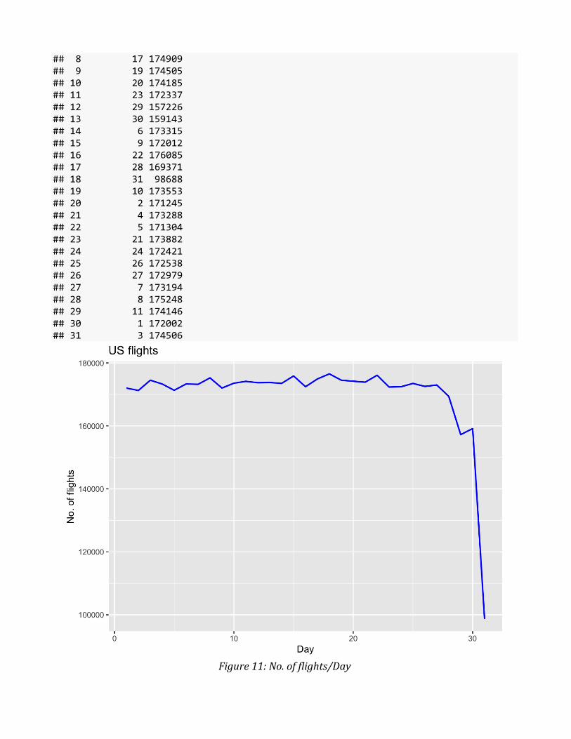
## 8 17 174909 ## 9 19 174505 ## 10 20 174185 ## 11 23 172337 ## 12 29 157226 ## 13 30 159143 ## 14 6 173315 ## 15 9 172012 ## 16 22 176085 ## 17 28 169371 ## 18 31 98688 ## 19 10 173553 ## 20 2 171245 ## 21 4 173288 ## 22 5 171304 ## 23 21 173882 ## 24 24 172421 ## 25 26 172538 ## 26 27 172979 ## 27 7 173194 ## 28 8 175248 ## 29 11 174146 ## 30 1 172002 ## 31 3 174506

Figure 11: No. of flights/Day

Prepare data for modelling

model_tbl <- flights_tbl %>% filter(ArrDelay >= 1) %>% mutate(ArrTime = as.double(ArrTime), AirTime = as.double(AirTime), DepDelay = as.double(DepDelay), ArrDelay = as.double(ArrDelay), CRSDepTime = as.double(CRSDepTime), CRSArrTime = as.double(CRSArrTime), CRSElapsedTime = as.double(CRSElapsedTime), TaxiIn = as.double(TaxiIn), TaxiOut = as.double(TaxiOut), DepTime = as.double(DepTime), ActualElapsedTime = as.double(ActualElapsedTime), Cancelled = as.double(Cancelled), NASDelay = as.double(NASDelay), Diverted = as.double(Diverted), SecurityDelay = as.double(SecurityDelay), LateAircraftDelay = as.double(LateAircraftDelay)) %>% mutate(hour = floor(CRSDepTime/100)) %>% mutate(gain = ArrDelay - DepDelay) %>% filter(!is.na(ArrDelay) & !is.na(DepDelay) & !is.na(Distance)) %>% filter(DepDelay > 5) %>% select(Origin, Dest, UniqueCarrier, FlightNum, Month, DayOfWeek, Distance, DepDelay, ArrDelay, AirTime, Cancelled, hour, gain) sdf_dim(model_tbl) ## [1] 1010795 13

glimpse(model_tbl) ## Observations: ?? ## Variables: 13 ## Database: spark_connection ## $ Origin <chr> "PHL", "PHL", "PHL", "PHL", "PIT", "STL", "CLT", "CLT",… ## $ Dest <chr> "CLE", "CLE", "CLE", "CLE", "PVD", "PIT", "BUF", "BUF",… ## $ UniqueCarrier <chr> "US", "US", "US", "US", "US", "US", "US", "US", "US", "… ## $ FlightNum <int> 724, 724, 724, 724, 725, 726, 728, 728, 729, 729, 729, … ## $ Month <int> 1, 1, 1, 1, 1, 1, 1, 1, 1, 1, 1, 1, 1, 1, 1, 1, 1, 1, 1… ## $ DayOfWeek <int> 7, 1, 7, 4, 5, 3, 6, 1, 7, 1, 6, 4, 1, 5, 7, 6, 3, 4, 4… ## $ Distance <int> 363, 363, 363, 363, 467, 553, 546, 546, 462, 462, 462, … ## $ DepDelay <dbl> 20, 14, 9, 7, 68, 14, 12, 20, 7, 7, 71, 34, 49, 21, 25,… ## $ ArrDelay <dbl> 36, 27, 57, 27, 58, 5, 8, 20, 38, 15, 87, 20, 54, 34, 2… ## $ AirTime <dbl> 64, 62, 67, 76, 70, 73, 69, 75, 83, 87, 93, 115, 106, 9… ## $ Cancelled <dbl> 0, 0, 0, 0, 0, 0, 0, 0, 0, 0, 0, 0, 0, 0, 0, 0, 0, 0, 0… ## $ hour <dbl> 7, 7, 7, 7, 16, 7, 9, 9, 11, 11, 11, 7, 16, 16, 16, 16,… ## $ gain <dbl> 16, 13, 48, 20, -10, -9, -4, 0, 31, 8, 16, -14, 5, 13, …

Analysing the delays through a geometric plot:

delay <- model_tbl %>% group_by(Origin) %>% summarise(count = n(), dist = mean(Distance, na.rm = TRUE), delay = mean(ArrDelay, na.rm = TRUE)) %>% filter(count > 20, dist < 2000, !is.na(delay)) %>% collect

Figure 12: Distance Vs. Delay

Partition into train and test for machine learning

partition <- model_tbl %>% sdf_random_split(training = 0.8, test = 0.2, seed = 2222) # Create table references data_training <- sdf_register(partition$train, "trips_train") data_test <- sdf_register(partition$test, "trips_test") # Cache tbl_cache(sc, "trips_train") tbl_cache(sc, "trips_test")

Linear Regression ## [1] "Took 12.14 secs to build a Linear Regression Model" ## [1] 3.064071 Gradient Boost Trees ## [1] "Took 8.8 mins to build a Gradient Boost Tree Model" ## [1] 19.1468 Extreme Gradient Boost Trees ## [1] "Took 9.05 mins to build an Extreme Gradient Boost Model" ## [1] 45.6706

Naive Bayes ## [1] "Took 4.87 secs to build a Naive Bayes Model" ## [1] 0.0243755 Decision Tree ## [1] "Took 26.98 secs to build a Decision Tree Model" ## [1] 26.07967 Random Forest ## [1] "Took 1.33 mins to build a Random Forest Model" ## [1] 60.60918 Calculating Lift, Gain, Accuracy, Performance Metrics and Feature Importance by Scoring Test Data

Figure 13: Lift Chart showing AUC

Figure 14: Bar Chart showing Accuracy

Convert the Spark data frame to H2O data frames

train_h2o <- as_h2o_frame(sc, data_training) test_h2o <- as_h2o_frame(sc, data_test) # Format H2O Data Frames train_h2o$Month <- as.factor(train_h2o$Month) train_h2o$DayOfWeek <- as.factor(train_h2o$DayOfWeek) train_h2o$Cancelled <- as.factor(train_h2o$Cancelled) train_h2o$FlightNum <- as.factor(train_h2o$FlightNum) test_h2o$Month <- as.factor(test_h2o$Month) test_h2o$DayOfWeek <- as.factor(test_h2o$DayOfWeek) test_h2o$Cancelled <- as.factor(test_h2o$Cancelled) test_h2o$FlightNum <- as.factor(test_h2o$FlightNum)

Now that we have converted the data to H2O data frame, we can train some models

Build H2O’s GLM, GBM, XGBoost & Random Forest models

Comparison of time taken to build models in H2O:

## [1] "Took 2.61 secs to build a General Linear Model." ## [1] "Took 13.66 secs to build a GBM." ## [1] "Took 2.18 mins to build a XGBoost Model." ## [1] "Took 1.05 mins to build a Random Forest Model." The RMSE & Mean Absolute Error (MAE) & Root Mean Square Error (RMSE) without cross validation:

## [1] "Mean Absolute Error of GLM : 10.082061737412" ## [1] "Mean Absolute Error of GBM : 9.85558905665857" ## [1] "Mean Absolute Error of XGBoost : 9.81981833233624" ## [1] "Mean Absolute Error of Random Forest : 11.7570684521862" ## [1] "RMSE of GLM : 16.4065469651842" ## [1] "RMSE of GBM : 16.0940898096046" ## [1] "RMSE of XGBoost : 15.9720172404345" ## [1] "RMSE of Random Forest : 19.2068432987401" Then we train another set of models on 80% of the data and cross-validated using 10 folds.

## [1] "Took 7.37 secs to build a 10 Fold Cross Validated GLM Model." ## [1] "Took 2.4 mins to build a 10 Fold Cross Validated GBM Model." ## [1] "Took 7.31 mins to build a 10 Fold Cross Validated XGBoost Model." ## [1] "Took 8.2 mins to build a 10 Fold Cross Validated Random Forest Model." Get the cross-validated Mean Absolute Error (MAE) & Root Mean Square Error (RMSE)

## [1] "Mean Absolute Error of GLM : 10.082061737412" ## [1] "Mean Absolute Error of GBM : 9.85558905665857" ## [1] "Mean Absolute Error of XGBoost : 9.83526414546222" ## [1] "Mean Absolute Error of Random Forest : 11.9411020068592" ## [1] "RMSE of GLM : 16.4065469651842" ## [1] "RMSE of GBM : 16.0940898096046" ## [1] "RMSE of XGBoost : 16.0178977247697" ## [1] "RMSE of Random Forest : 19.4247691520044"

Score H2O test data and comparison of the root mean squared error for each model:

Figure 15: RMSE comparison for different models in H2O

4.4 Deployment

For this research, a reactive shiny application is roughly adapted from

https://github.com/SavageDoc/BreakingTheBottleneck-Sydney to deploy the machine learning

models. This shiny application is divided into a sidebar and a main panel.

The sidebar enables the user to tweak various parameters such as seed, input variables, train

percentage as well as configuration of machine learning models such as Linear, Random Forest and

XGBoost. The sidebar also provides option to select the number of folds for cross validation, make

decision on which model to implement for the purpose of generating report and select the origin and

destination airports to view the respective gain chart, data and map.

The main panel is further divided into 10 tabs, namely, Summary, Full Data Plot, Train, Test,

Cross Validate, Gain Chart, Gain Data, Variable Importance, Map and Report. As the name suggests,

the Summary page is an Rmarkdown document which gives a brief summary of the default

parameters considered and the results. The Full Data Plot tab shows the correlation plot of all the

variables in the dataset. The Train, Test and CV tabs shows the comparison plot of the train, test and

cross validation results across Linear Regression, Random Forest and XGBoost models. The Gain

Chart, Gain Data and Map tabs show the respective predicted gain vs observed gain between any

origin and destination as well as a geographical map showing the flight path. The Variable Importance

tab shows which variable has highest importance based on the XGBoost model. The Report tab does

not have much going on the main panel as it is mostly linked to background activity. Instead it shows

a message “Slides Generated”, once the report is generated.

4.5 Operate & Optimise

With the available hardware in hand, this research has demonstrated the improvement of

machine learning model generation performance by employing Sampling, Profiling, Scaling Out,

Pipelines and H2O.ai in SparklyR.

It is proved that H2O.ai improves performance and reduces cost compared to Spark in R, as

the time taken to build models in H2O.ai is considerably less than SparklyR. Also, GBM and XGBoost

models in H2O.ai are found to be the best machine learning models compared to Random Forest and

GLM with the lowest RMSE scores of 257.1191 and 256.4002 respectively. But in terms of hardware

cost and performance, H2O.ai XGBoost is very costly as it takes 7.31 minutes to build a 10-fold cross

validated model where as it takes just 2.3 minutes for the same in case of H2O.ai GBM model.

Limitations

This research is limited by the hardware used for modelling. Scaling Up the hardware

configuration by the addition of dedicated Graphics Memory and GPUs would have considerably

improved the performance of all models as well as allowed to handle much larger datasets preferably

of Big Data proportions. Scaling up hardware would also allow the implementation of additional

machine learning models such as Artificial Neural Networks.

This research can also be expanded to the integration of H2O.ai with RShiny which will

potentially allow the processing of Big Data directly on RShiny. Also, this research is limited by the

fact that at this current stage of R, it is not possible to perform Machine Learning directly on a

pipeline model. It is heartening to note that, this feature is currently under development at RStudio

Inc. and can be realized in the near future.

Conclusion and Future Work

H2O.ai and Spark in R provide a distinct advantage when dealing with large datasets or

streaming data. The availability of pipelines enable to reduce cost considerably by improving

processing speed and performance. This research has shown that integration of SparklyR and H2O.ai

improves Machine Learning performance even with a mediocre hardware configuration. All the

research objectives, namely, integrating R, Spark, H2O.ai and Shiny, enhancing machine learning

speed by using H2O.ai, calculation of time and resources saved by integrating H2O.ai with Spark in R,

addressing the challenges to integrate Spark in R with Shiny and integrating RMarkdown with Shiny

to generate report templates were met. The time gained has been predicted with high accuracy while

maintaining very low RMSE and report generation was achieved by collaborating between

technologies to reduce rework and improve efficiency. Therefore the hypothesis that Spark

Streaming improves performance of machine learning models and RMarkdown can generate

PowerPoint slides from Shiny stands proved.

During the implementation, the ASUM-DM methodology has been studied and the steps that

have been applied for this research was proposed for the implementation of different technologies

such as Spark, H2O.ai, Shiny and RMarkdown to find the best way to integrate them. This study on

machine learning technologies demonstrates that H2O.ai improves performance measures on the

hardware cost problem. This proposed methodology can be used for different analytical studies and

machine learning models. For future studies, dedicated Graphics Memory and GPUs could be added

to improve on the current performance figures. Also, option can be given in the Shiny application to

allow the upload of any dataset and apply different machine learning models on it.

References / Bibliography

Dataset from American Statistical Association [Online]. Available at:

http://stat-computing.org/dataexpo/2009/the-data.html, (Accessed 5, May, 2019)

“A machine learning approach for prediction of on-time performance of flights” – by

Balasubramanian & others. IEEE [Online]. Available at:

https://ieeexplore.ieee.org/document/8102138, (Accessed 5, June, 2019)

“Artificial Intelligence and Machine Learning in Aviation”. IATA [Online]. Available at:

https://www.iata.org/events/Documents/ads18-ai-lab.pdf, (Accessed 9, June, 2019)

“Predictive Modelling of Aircraft Flight Delay” – by Anish M. Kalliguddi , Aera K. Leboulluec, Universal

Journal of Management. RPUBS [Online]. Available at:

http://www.hrpub.org/download/20171130/UJM3-12110417.pdf, (Accessed 22, June, 2019)

“Application of Reinforcement Learning Algorithms for Predicting Taxi-out Times” – by Poornima

Balakrishna, Ph.D. Candidate, Rajesh Ganesan,Ph.D., Lance Sherry, Ph.D. ATM [Online]. Available at:

https://catsr.vse.gmu.edu/pubs/ATM2009_TaxiOut.pdf, (Accessed 21, June, 2019)

“Application of Machine Learning Algorithms to Predict Flight Arrival Delays” – by Nathalie Kuhn and

Navaneeth Jamadagni. Stanford [Online]. Available at:

http://cs229.stanford.edu/proj2017/final-reports/5243248.pdf, (Accessed 17, June, 2019)

“How Big Data in Aviation Is Transforming the Industry” – by Danny Bradbury. Horton Works [Online].

Available at:

https://hortonworks.com/article/how-big-data-in-aviation-is-transforming-the-industry/,

(Accessed 14, June, 2019)

“How will AI help us predict disruption in air travel?” – by Stephane Cheikh, Artificial Intelligence

Program Director, SITA [Online]. Available at:

https://www.sita.aero/resources/blog/how-will-ai-help-us-predict-disruption-in-air-travel,

(Accessed 15, June, 2019)

“The Evaluation of Ensemble Sentiment Classification Approach on Airline Services Using Twitter” –

by Zechen Wang. DIT [Online]. Available at:

https://arrow.dit.ie/cgi/viewcontent.cgi?article=1108&context=scschcomdis,

(Accessed 18, July, 2019)

“AI WIELDS THE POWER TO MAKE FLYING SAFER—AND MAYBE EVEN PLEASANT” – by Eric Adams.

Wired [Online]. Available at:

https://www.wired.com/2017/03/ai-wields-power-make-flying-safer-maybe-even-pleasant/,

(Accessed 10, June, 2019)

“Understanding Customer Choices to Improve Recommendations in the Air Travel Industry” – by

Alejandro Mottini & others. CEUR-WS [Online]. Available at:

http://ceur-ws.org/Vol-2222/paper6.pdf, (Accessed 12, June, 2019)

“Applications Of Machine Learning” – by Harshani Chathurika. Available at:

https://medium.com/swlh/applications-of-machine-learning-9f77e6eb7acc,

(Accessed 11, June, 2019)

“7 Ways Airlines Use Artificial Intelligence and Data Science to Improve Operations”- by Kateryna

Lytvynova. Datafloq [Online]. Available at:

https://datafloq.com/read/ways-airlines-artificial-intelligence-data-science/5309,

(Accessed 21, June, 2019)

“R and Spark: How to Analyze Data Using RStudio's Sparklyr and H2O's Rsparkling Packages: Spark

Summit East talk” - by Nathan Stephens. SlideShare [Online]. Available at:

https://www.slideshare.net/SparkSummit/r-and-spark-how-to-analyze-data-using-rstudios-sparklyr-

and-h2os-rsparkling-packages-spark-summit-east-talk-by-nathan-stephens, (Accessed 28, June, 2019)

“Characterization and prediction of air traffic delays” – by J. J. Rebollo and H. Balakrishnan.

Transportation Research Part C: Emerging Technologies, 44(Supplement C):231–241, July 2014

[Online]. Available at:

http://www.mit.edu/~hamsa/pubs/RebolloBalakrishnanTRC2014.pdf, (Accessed 17, June, 2019)

“A systems approach for scheduling aircraft landings in JFK airport” – by S. Khanmohammadi, C. A.

Chou, H. W. Lewis, and D. Elias. In 2014 IEEE International Conference on Fuzzy Systems (FUZZ-IEEE),

pages 1578–1585, July 2014 [Online]. Available at:

https://ieeexplore.ieee.org/document/6891588, (Accessed 18, June, 2019)

“Estimating Taxi-out times with a reinforcement learning algorithm” – by P. Balakrishna, R. Ganesan,

L. Sherry, and B. S. Levy. In 2008 IEEE/AIAA 27th Digital Avionics Systems Conference, pages 3.D.3–1–

3.D.3–12, Oct. 2008 [Online]. Available at:

https://ieeexplore.ieee.org/document/4702812, (Accessed 10, June, 2019)

“Forty years of S” – by Rick Becker, Channel 9, MSDN [Online]. Available at:

https://channel9.msdn.com/Events/useR-international-R-User-conference/useR2016/Forty-years-of-

S, (Accessed 18, July, 2019)

Santiago Angee, Silvia I. Lozano-Argel, Edwin N. Montoya-Munera, Juan-David Ospina-Arango, Marta

S. Tabares-Betancur. (2018) ‘Towards an improved ASUM-DM process methodology for cross-

disciplinary multi-organization Big Data & Analytics projects’, Directory of Research Gate [Online].

Available at:

https://www.researchgate.net/publication/326307750_Towards_an_Improved_ASUM-

DM_Process_Methodology_for_Cross-Disciplinary_Multi-

organization_Big_Data_Analytics_Projects_13th_International_Conference_KMO_2018_Zilina_Slovak

ia_August_6-10_2018_Proceeding, (Accessed 18, June, 2019)

IBM Analytics Solutions Unified Method, Available at:

http://gforge.icesi.edu.co/ASUM-DM_External/index.htm#cognos.external.asum-

DM_Teaser/deliveryprocesses/ASUM-

DM_8A5C87D5.html_desc.html?proc=_0eKIHlt6EeW_y7k3h2HTng&path=_0eKIHlt6EeW_y7k3h2HTn

g, (Accessed 19, June, 2019)

“Mastering Spark with R” by Edgar Ruiz, Kevin Kuo, Javier Luraschi. Oreilly [Online]. Available at:

https://www.oreilly.com/library/view/mastering-spark-with/9781492046363/

(Accessed 15, August, 2019)

“Breaking the Bottleneck” by Craig Savage. Github [Online]. Available at:

https://github.com/SavageDoc/BreakingTheBottleneck-Sydney

Appendix This section will show the contents of the Artefacts and the steps to implement the R code for

dissertation project titled “Performance Improvement and Reporting Techniques using H2O.ai and

SparklyR”.

Contents of the Artefacts

1. Dataset:

2002.csv

2. R Codes and Results:

• RSparkling: Data loading codes to SparklyR

• EDA_RSparkling: Exploratory data analysis on neo4j with python

• ML_RSparkling: Machine learning & Accuracy code for SparklyR

• H2O_RSparkling: Machine Learning in H2O code

• Rsparkling_Shiny: RShiny App code

3. Documents Folder: Sample templates for RShiny application and the output directory for

generated reports