Documento de TrabajoISSN (edición impresa) 0716-7334

ISSN (edición electrónica) 0717-7593

Comparing the net benefits of incentive based and command and control regulations in a developing context: the case of Santiago, Chile

Raúl O´RyanJosé Miguel Sánchez

Nº 221Agosto 2002

www.economia.puc.cl

COMPARING THE NET BENEFITS OF INCENTIVE BASED AND COMMAND AND CONTROL REGULATIONS IN A DEVELOPING CONTEXT:

THE CASE OF SANTIAGO, CHILE1

Raúl O’Ryan Center for Applied Economics

Universidad de Chile

José Miguel Sánchez Instituto de Economía

Pontificia Universidad Católica de Chile

August 2002

1 We would like to tank Juan Pablo Montero for many useful comments; Rodrigo Bravo and Carlos Holz for excellent research assistance. This paper was was presented at the Second World Congress of Environmental and Resource Economists.

2

COMPARING THE NET BENEFITS OF INCENTIVE BASED AND COMMAND AND CONTROL REGULATIONS IN A DEVELOPING CONTEXT:

THE CASE OF SANTIAGO, CHILE

Raúl O’Ryan Center for Applied Economics

Universidad de Chile

José Miguel Sánchez Instituto de Economía

Pontificia Universidad Católica de Chile

Abstract

There are numerous studies that establish the magnitude of the static efficiency gains made

possible through the use of a cost effective ambient permit system (APS) compared to

command and control (CAC) or other suboptimal instruments such as an emission permit

system (EPS). However the cost effectiveness of APS rests both on the efficiency gains related

to equalizing marginal costs of reduction and a lower degree of required control. As a result of

this latter factor, CAC and EPS generally impose concentration reductions higher than

required by the target air quality standard and also by APS. In developing contexts, as a result

of high levels of pollution and only recent introduction of control policies, health benefits of

reducing pollution significantly can be expected to be high whereas the costs may still be

relatively low. Consequently the excess reductions may produce net benefits -benefits of

improved air quality minus compliance costs-. This paper evaluates for Santiago whether

reduced concentrations below the level of the standard as a result of suboptimal policies result

in health improvements that produce greater net benefits than incentive based approaches. The

results show that considering uniform air quality targets and for the range of technologically

plausible control options in Santiago, suboptimal CAC and EPS policies result in higher net

benefits than APS.

JEL Classification, Q25

3

1. INTRODUCTION

There are numerous studies based on simulation models which establish the magnitude of the

static efficiency gains made possible through the use of marketable permits for fixed sources

compared to command and control (CAC) instruments2. In a developing country context,

O’Ryan (1996), established the cost reductions from using ambient based tradeable permits

(APS). These studies suggest that in most cases the cost reductions of APS over CAC are

substantial. An important caveat however is that many of these reductions are the result of

lower emission reduction requirements under an optimal APS, i.e. APS, while complying with

a given air quality standard in all receptors, allows more emissions than other instruments in

non binding receptors. The cost effectiveness of APS rests then both on the efficiency gains

related to equalizing marginal costs of reduction – a true efficiency gain – and a lower degree

of required control (Tietenberg(1985)).

As many have pointed out (see for example Tietenberg (1985) and Oates et al. (1989)), if

there is no value assigned to this overcontrol3 CAC instruments will not improve at all on

incentive based approaches and will indeed be more expensive. If “however, reduced

concentrations below the level of the standards bring with them improvements in health or the

environment, CAC approaches will produce greater benefits than incentive based approaches”

(Oates et al. (1989), p.1233) . Consequently the comparison among instruments without

correcting for these benefits is unfair and may be misleading. Considering the fact that most of

the time regulators propose air quality standards that are uniform and not socially optimal, it

may be the case that suboptimal CAC policies will result in higher net benefits (benefits of

improved air quality minus compliance costs).

To overcome this problem there are two approaches. One is to eliminate the “lower degree of

required control component” by imposing on all instruments the compliance with the same air

2 See for example: Atkinson and Lewis (1974), Hahn and Noll (1982), Krupnick (1986), Mc Gartland and Oates (1984), Portney(1990), Seskin, Anderson,and Reid (1983 and Spofford and Paulsen(1988). 3 The problem is that cost effective approaches implicitly assign a shadow price of zero to improvements that exceed the standard .

4

quality in all receptor locations, as is done in O’Ryan (1996)4. A second is to determine the

net benefits, i.e., the difference between the costs and benefits, for each instrument, allowing a

more complete comparison.

This paper evaluates the net benefits associated to the use of market-based incentives (MBIs)

and CAC policies to control TSP emissions from fixed point sources5 in Santiago, Chile. The

authors are aware of only one paper that undertakes this comparison for the US (Oates et. al

(1989)) and none for developing contexts. The results shed light as to the importance of

including both costs and benefits in the comparison of different regulatory instruments, in

particular in developing contexts where costs of reduction are not too high yet because little

control effort has been undertaken, and correspondingly health benefits of improving air

quality are high. The second section presents an overview of the air pollution problem in

Santiago. The third section addresses the compliance costs of reaching given air quality

targets using MBIs and CAC instruments. Using a linear programming model, the total costs

of achieving a desired air quality standard have been established for each policy. The fourth

section presents the population based health benefits associated to each instrument. Section

five compares the net benefits of applying APS and two second best policies. The last section

presents the main conclusions and future research lines.

2. The Air Pollution Problem in Santiago.

The city of Santiago, Chile, like many large cities in developing countries, suffers critical air

pollution problems. In particular, in winter the concentrations of total suspended particulates

(TSP) and smaller PM-10 particulates constantly exceed the established ambient standards.

Significant adverse health effects on the city’s 5.2 million inhabitants, associated with the high

levels of pollution by PM10 in winter, have been established (Ostro et. al (1996), Ostro et. al

(1999)). Additionally, ozone pollution is significant in spring and summer. The city's policy-

makers have been struggling since the beginning of the nineties to improve air quality,

objective that would require reducing emissions to approximately half the current levels to

4 In practice this is done by running a model with a command and control instrument, and using the vector of air quality obtained as the targets to be met by APS. 5 Point sources are sources that emit a gas flow greater than 1000 m3N per hour, through a chimney.

5

reach the desired air quality targets6. Although they have been successful in halting the

increase in pollution that could have been expected due to the significant increase in economic

activity in the city during the decade, air quality is still far from the target as can be seen in the

following figure.

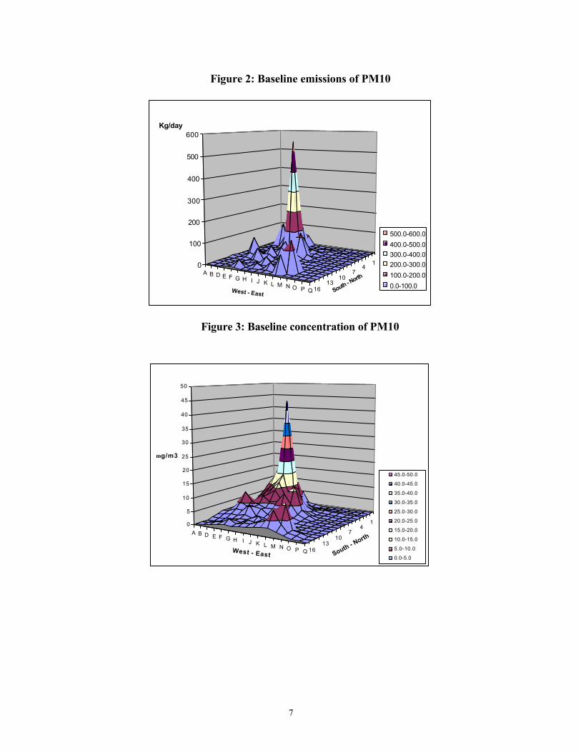
To examine the spatial configuration of emissions from fixed point sources in Santiago, the

city can be divided into a 34 x 34 km grid. The grid comprises 289 (2 x 2 km) cells which

contain the relevant sources of the air pollution problem in Santiago, as well as most of the

exposed population. In this area there is a total of 1098 fixed point sources. Total TSP

emissions in the city reached 2.55 tons/day in 1998 . Figure 2 presents average daily PM10

emissions, measured in kilograms per day, from each cell in the grid, for 1999. Clearly,

polluting sources are clustered in a few specific zones. The cell with highest emissions is

located in the northwestern part of the city and emits 594 Kg/day, 22 % of the total PM10

emitted in the city7. Of the 289 cells of the grid, only seven are highly polluting8, and the

fourteen most polluting cells emit 65% of total emissions. These emissions spread out

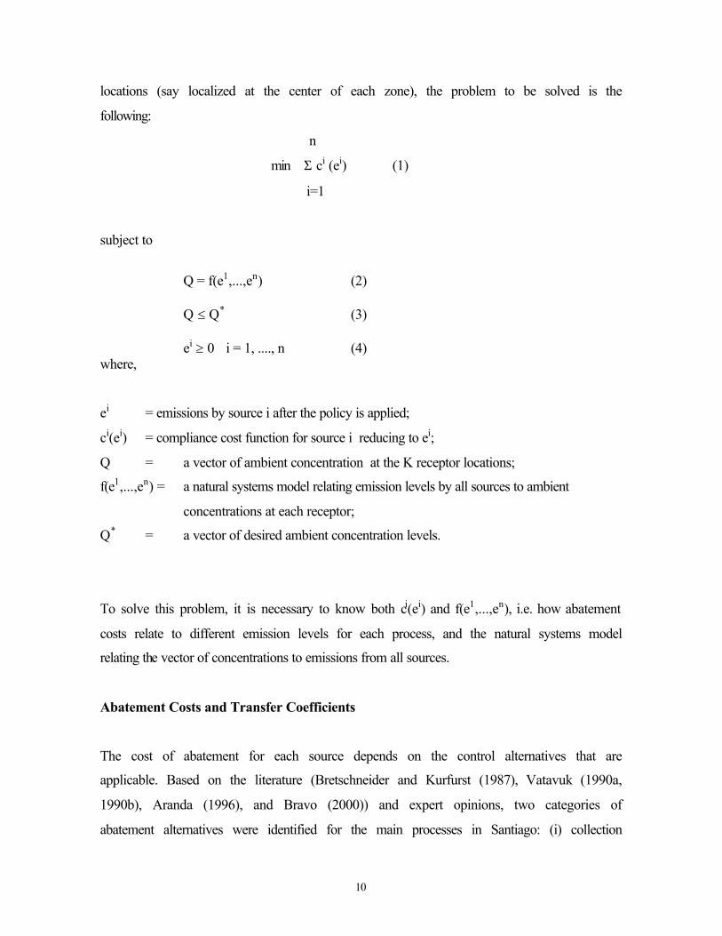
smoothly to the rest of the city affecting air quality in each cell. Figure 3 presents the

corresponding concentrations levels, measured in (µg/m3) in each cell. The daily PM10

standard is 150 (µg/m3), that cannot be exceeded more than once in a year. The USEPA

annual standard of 50 (µg/m3) which will become an official standard in Chile by year 2012

can be used for purposes of comparison.

6 Set, as is usual, based on health effects, not cost-benefit analysis. 7 In this cell there is a power station with both natural gas and diesel powered generators. 8 Emit more than 3% of total emissions.

6

Figure 1: Air Quality in Santiago 1989-1999, PM-10.

7

Figure 2: Baseline emissions of PM10

14

710

1316

A B D E F G H I J K L M N O P Q

0

100

200

300

400

500

600Kg/day

South - North

West - East

500.0-600.0

400.0-500.0300.0-400.0200.0-300.0

100.0-200.0

0.0-100.0

Figure 3: Baseline concentration of PM10

14

710

1316

A B D E F G H I J K L M N O P Q

0

5

10

15

20

25

30

35

40

45

50

µ g/m3

South - North

West - East

45.0-50.0

40.0-45.0

35.0-40.0

30.0-35.0

25.0-30.0

20.0-25.0

15.0-20.0

10.0-15.0

5.0-10.0

0.0-5.0

8

The main polluting sources of PM10 are summarized in Table 1. Industrial processess are the

main emission sources, corresponding to 55 % of total emissions, while industrial boilers

account for 40% the total. Heaters are also significant contributors (5%). The main emitting

fuels are natural gas9 and particles emitted by industrial processes using electricity10. Diesel

oil is also an important source of emissions.

Table 1 Percentage of PM-10 Emissions by Source Category and Fuel

Ele

ctri

city

Coa

l

Woo

d

Fue

l 6

Fue

l 5

Die

sel

Nat

ural

Gas

Total

Industrial

processes 30,64% 1,13% 0,04% 1,03% 0,42% 3,65% 18,24% 55,1%

Boilers 0,00% 0,65% 0,57% 0,45% 5,70% 15,07% 17,53% 40,0%

Heaters 0,00% 0,00% 0,02% 0,00% 1,70% 2,12% 0,89% 4,7%

Bakeries 0,00% 0,00% 0,00% 0,00% 0,00% 0,13% 0,02% 0,16%

TOTAL 30.64% 1.78% 0.63% 7.48% 12.82% 22.97% 36.68% 99.24%

Source: Bravo ( 2000).

The main instruments used to control air pollution have been command and control: emission

standards for industry, homes and new cars, as well as the elimination of highly polluting

buses and increasingly tighter emission standards for diesel motors. For fixed point sources,

these standards allowed reducing emissions from 9 tons per day in 1994, to approximately 2.6

tons in 199811.

There have been lukewarm attempts to introduce flexibility for fixed point sources through the

introduction of an offset system for particulates. The system set an emission standard for all

existing point sources and allows them to trade any excess reductions. New fixed point

sources (entering the city after 1992), are required to offset all their emissions and recently are

being required to offset 120% . Trades are undertaken on a one to one basis (i.e. it is an

emission permit system, EPS) even though it is recognized that particulates behave as a non-

uniformly mixed pollutant.

9 There is a mega-source that generates electricity within the city limits, that uses natural gas and emits by itself, almost 11% of total PM10 emissions in the city. 10 The emissions are not generated by the energy source in this case, but are due to the characteristics of the process (smelters for example). 11 These numbers must be taken as a reference only. In particular the figure for 1994 is an estimation that is not based on actual measurements of emissions.

9

The offset system has not worked as expected12. There have been very few trades most of

them internal to each firm, and as a result the market has not fully developed. Additionally, the

introduction of natural gas as a new fuel in the city in 1997, has reduced the costs of

decreasing emissions dramatically for many sources, to the point where it is economically

convenient for many to switch to this clean fuel that allows them to comply with the emission

standard. Some regulators are concerned that allowing one-to-one trades can result in hot

spots.

Finally, in the last two years, the industrial sector has become increasingly vocal about the

need to stop pressing for more restrictions to fixed sources, arguing that they have reduced

their contribution to air pollution significantly since the beginning of the nineties, while other

sectors have not.

Consequently the question addressed in this paper is given that there is a national air quality

standard established not by cost benefit considerations, is there an advantage, from a cost-

benefit perspective, of using marketable permits, in particular an ambient permit system

(APS), in Santiago? Or is it appropriate in the current situation to use simpler EPS or even

command and control instruments?

3. Compliance Costs of Improving Air Quality Under Different Policies

This section presents the model developed to evaluate compliance costs and the main

results related to the costs of applying MBIs and CAC policies in Santiago .

The Problem

From a cost-effectiveness perspective, the regulator's problem is to obtain the desired air

quality in each receptor location at a minimum cost. Considering there are n polluting

sources, K zones in which emissions are generated, and the same number of receptor

12 The main reason for this have been implementation failures. For a performance evaluation of the Offset system in Santiago see Montero, J.P. et. al (2002).

10

locations (say localized at the center of each zone), the problem to be solved is the

following:

n

min Σ ci (ei) (1)

i=1

subject to

Q = f(e1,...,en) (2) Q ≤ Q* (3) ei ≥ 0 i = 1, ...., n (4) where,

ei = emissions by source i after the policy is applied;

ci(ei) = compliance cost function for source i reducing to ei;

Q = a vector of ambient concentration at the K receptor locations;

f(e1,...,en) = a natural systems model relating emission levels by all sources to ambient

concentrations at each receptor;

Q* = a vector of desired ambient concentration levels.

To solve this problem, it is necessary to know both ci(ei) and f(e1,...,en), i.e. how abatement

costs relate to different emission levels for each process, and the natural systems model

relating the vector of concentrations to emissions from all sources.

Abatement Costs and Transfer Coefficients

The cost of abatement for each source depends on the control alternatives that are

applicable. Based on the literature (Bretschneider and Kurfurst (1987), Vatavuk (1990a,

1990b), Aranda (1996), and Bravo (2000)) and expert opinions, two categories of

abatement alternatives were identified for the main processes in Santiago: (i) collection

11

devices such as cyclones, multicyclones, bag filters and wet scrubbers; and (ii), for some

sources, a change of fuel. To estimate the costs of collection devices, the net discounted

cash flow of total capital investments and net annual operating costs incurred each year

over the useful life of the equipment were estimated. To estimate the present value of

switching to cleaner fuels, the cost of transformation and the cost differential associated

with using a different fuel were estimated. Different sized control devices were costed. As a

result, analytical cost relations were established for each control alternative (see appendix

1). These costs depend on the size of the source (gas flow) and hours of operation. Each

control option was also assigned the abatement efficiency presented in the following table,

based on expert opinion.

12

Table 2: Control Efficiencies of Abatement Options for Main Processes in

Santiago (in Percentage)

Process

Cyc

lone

s

Mul

ticy

clon

es

Bag

Filt

ers

Ven

turi

Scru

bber

s E

lect

rost

atic

Pre

cipi

tato

rs

Swit

ch to

Fue

l

Oil

5 Sw

itch

to F

uel

Oil

6 Sw

itch

to

Die

sel

Swit

ch to

gas

Coal Heaters and Boilers 33 70 99 96 97 65 80 94 99

Wood Heaters and Boilers 15 50 99 89 95 63 79 94 99

Fuel Oil 6 Heaters and Boilers 5 30 99 86 94 - 43 83 97

Fuel Oil 5 Heaters and Boilers 5 30 99 86 94 - - 69 94

Diesel Heaters and Boilers 5 30 99 86 94 - - - 86

Coal Furnace 40 82 99 98 99 - - - -

Wood Furnace 15 50 99 89 95 - - - -

Fuel Oil 6 Furnace 5 30 99 86 94 - 43 83 97

Fuel Oil 5 Furnace 5 30 99 86 94 - - 69 94

Diesel Furnace 5 30 99 86 94 - - - 88

Al, Cu, Br Foundries 31 80 99 95 90 - - - -

Stone and Grain Crushing 41 85 99 98 91 - - - -

Stone and Grain Cleaning 35 60 99 98 98 - - - -

Asphalt Plants 40 89 99 97 94 - - - -

Source: Aranda (1996), page33.

13

To relate concentrations to emissions, the natural systems model is substituted by an

environmental "transfer" coefficient, αik, relating changes in emissions by source i to

changes in concentration at receptor k. To obtain these coefficients a simplified "cell"

dispersion model, available for Santiago, was used. The wind fields had to be averaged

over the day for this, and meteorological conditions which reflected episode conditions had

to be selected13. Twenty two episode days were used and the corresponding transfer

coefficients averaged. As a result, the transfer coefficients obtained reflect the impact of a

unit of emissions on concentration levels in each cell of the grid, for adverse meteorological

conditions. The results, which were surprising because it was previously thought (by

whom?) that the main impacts were in a different direction, are presented in Appendix 2.

The Policies Evaluated

With information on emissions, location of each source, costs of abatement for each

individual source and the transfer coefficients, the overall costs of two MBI policies and

one CAC policy were evaluated. The policies considered for this exercise were:

(i) The spatially-differentiated ambient permit system (APS). Under this policy, per-

mits defined in units of concentration at each receptor, are distributed so as to achieve the

desired air quality goal at each receptor which corresponds to the air quality standard valid

nationwide.

(ii) A marketable emission permit system (EPS). Under EPS, total allowable

emissions from fixed sources in the airshed are established. Permits, equivalent to these

emissions, are distributed to polluters, who can then buy and sell the permits from any part

of the city on a one-to-one basis.

(iii) A uniform concentration standard for all sources (STD). All point sources are

required to emit at concentrations lower than a single concentration standard.

13 Episode days are those in which the air quality standard is exceeded.

14

To compare the costs of different policies, the most widely used criterion are the

compliance costs, under each policy, of meeting a uniform concentration standard at all

receptor locations in the city (each cell of the grid in this case). Any policy must at least

reach this standard everywhere. This is the success criterion used in this section. Allowed

concentrations ranging from as low as 5% of current concentration in the cell with highest

concentration , to as high as 47% were evaluated. Reductions higher than 47% are not

possible in the worst receptor location without reducing activity of some sources or closing

them down, option that has not been considered in this study.

Compliance Costs Under Different Policies

The compliance costs and reductions in allowed concentrations at the worst receptor

location(s), under each of the three policies, resulting from different expenditure levels by

fixed sources in Santiago are presented in Figure 4. The recent introduction of natural gas

as a control option clearly imposes some surprising results. First, many sources that have

not switched to natural gas could do so and actually obtain net benefits, i.e. their total

production costs would fall. The explanation for this is that at current prices, many sources

using diesel and fuel oil for combustion processes, can switch to natural gas and produce

the same amount of energy at a lower cost. This lower operating cost (discounted over

twenty years) covers the required transformation cost, and the source actually obtains net

benefits. Consequently 32% of current emissions could be reduced if all those firms that

can switch with net benefits, do so14.

14 Not all the sources had immediate access to the natural gas since time passed between the arrival of the natural gas in 1997 and the development of the distribution network.

15

Figure 4:

Source: Bravo (2000).

Note: $460= 1US$ (1998).

Second, as expected APS is clearly the most cost-effective instrument. Moreover, over the

whole range of reduction, total costs are negative15 for this instrument. A fully operating

APS policy would take full advantage of the win-win situation discussed before, obtaining

significant net benefits. The maximum 47% reduction can be obtained with yearly net

benefits of approximately US$13 million. The suboptimal spatially undifferentiated EPS

system on the other hand would impose a significant cost of over US$28 million per year to

15 Obviously marginal costs are not however. They increase steadily over the reduction range.

Compliance Costs of Abatement for Different Policy Instruments

47%

36%

47%

47%

36%

-30,000

-20,000

-10,000

0

10,000

20,000

30,000

30% 32% 34% 36% 38% 40% 42% 44% 46% 48% 50%

Percentage reduction in concentrations relative the worst cell

To

tal C

ost

MU

S$/

year

APSEPSSTD

16

reach a maximum level of 47% of the current concentration at the worst receptor location.

STD can only impose a 41% reduction at the worst receptor location, because it is assumed

that the authority can only impose undifferentiated standards. Within the range of reduction

of this instrument, it is clearly more costly than EPS16.

Air Quality In Each Receptor Location

Even if APS is the most cost effective policy, and both EPS and STD are much more

costly, much of the cost reduction is not related to gains in efficiency but to the lower

degree of required control component. Figure 5 presents the concentration reached in every

cell with each instrument when a maximum concentration reduction of 36% with respect to

the worse cell is imposed. As expected, as a result of APS, concentrations are higher than with

both EPS and STD. For example, considering a cut all along the J cell presented in figure 6, it

can be observed that APS allows higher concentrations in all cells relative to the other two

instruments. EPS imposes the highest reductions.

16 It must be borne in mind that negative total costs does not mean that all sources gain switching to gas. Actually, many individual sources have to incur in high costs to reduce emissions.

17

Figure 5: Air Quality Resulting from A 36% Reduction Target Considering Different

Policy Instruments

14

710

1316

A B D E F G H I J K L M N O P Q

0

5

10

15

20

25

30

35

40

45

50

South - North

West - East

Concentrations in each cell considering APS policy and

a 36% reduction target

[µ g/m3 ]

45.0-50.0

40.0-45.0

35.0-40.0

30.0-35.0

25.0-30.0

20.0-25.0

15.0-20.0

10.0-15.0

5.0-10.0

0.0-5.0

147

1013

16

A B D E F GH I J K L M N O P Q

0

5

10

15

20

25

30

35

40

45

50

South - North

West - East

Concentrations in each cell considering an EPS policy

that reaches a 36% reduction target[µ g/m3]

45.0-50.0

40.0-45.0

35.0-40.0

30.0-35.0

25.0-30.0

20.0-25.0

15.0-20.0

10.0-15.0

5.0-10.0

0.0-5.0

14

710

1316

A B D E F G H I J K L M N O P Q

0

5

10

15

20

25

30

35

40

45

50

South - North

West - East

Concentrations in each cell considering an STD policy that reaches a 36% reduction target

[µg/m3]

45.0-50.0

40.0-45.0

35.0-40.0

30.0-35.0

25.0-30.0

20.0-25.0

15.0-20.0

10.0-15.0

5.0-10.0

0.0-5.0

18

Figure 6

Comparison of Air quality levels reached in each cell (a long the j axis) with each policy instrument, considering a reduction of 36%

0.0

2.0

4.0

6.0

8.0

10.0

12.0

1 2 3 4 5 6 7 8 9 10 11 12 13 14 15 16 1 7

Cells

Air

qual

ity [

g/m

3]

APS

EPS

STD

As a consequence, the health benefits from applying each instrument should be different,

since the concentration reductions are different. These benefits are evaluated in the

following section.

4. The Health Benefits of Improved Air Quality.

In this section we present the value of the population weighted health effects of improving

air quality with each of the three instruments discussed before. The estimation of the

benefits associated with air quality improvements has considerable difficulties due to fact

that clean air is a non-market good and hence one for which there is no information

available on prices and/or quantities traded in order to estimate a proper monetary measure

for welfare changes. In this paper we followed the indirect method or dose – response

function approach ,a methodology frequently used in environmental benefit estimation and

specially to estimate health related benefits (see for example [Externe (1999)]). The

methodology involves three stages:

19

Stage 1 : The impact on concentrations that result from the application of each policy

instrument has to be estimated. The change of concentrations with and without the project

is given by:

∆q = q(s1) - q(s0)

where ∆q is the reduction in the concentrations of pollutants (for example, PM10) and the

vectors s1 and s0 correspond to the environmental policies to be evaluated (s1) and those in

place in the original situation (s0). The function q(.), corresponds, in general, to a pollutant

dispersion model that predicts the behavior of concentrations as a result of the change in

emissions that result from the policies included in s over the different sources. These results

are presented in the previous chapter.

Stage 2 : The effects that pollutant concentration reduction have on different health

outcomes have to be estimated. The change in the health effects are quantified using dose –

response functions for a set of health effects for which there are well established statistical

relations in the environmental epidemiological literature. These dose-response functions are

applied to the exposed population to determine the population weighted health effects. For

this, the exposed population in each cell is considered.

Stage 3: Lastly, the health effects found in stage 2 have to be valued in monetary units and

they have to be summed up over the different effects, over the individuals exposed and over

time since the benefits occur through time. In other words, the benefits associated with the

environmental policy or project evaluated are estimated as the avoided costs due to the

reduced cases of mortality and morbidity due to it. In this section we consider the

population weighted health effects related to the average PM-10 concentration in each cell,

resulting from each policy.

Dose-Response Functions.

The use of dose - response functions to estimate health effects can be described with the

20

following equation in which the estimated impact in the health effect that is being analyzed

(hospital admissions, mortality, etc.) is given by :17

(1) dHi = b * POPi * dA

where:

dHi = change in the risk of the health effect i in the population under exposure.

b = slope of the dose-response function.

POPi = population exposed and under risk of being affected by effect i

dA = change in atmospheric pollution for the pollutant under consideration.

Dose- response functions come from environmental epidemiology studies in which the aim

is to try to estimate the health effects that can be attributed to atmospheric pollution after

controlling for the effect of other variables on the probability of suffering health effects:

like nutrition habits, smoking habits, temperature, time spent outdoors, supply of medical

services, etc. Ideally the dose-response functions used for benefit estimation should be

estimated with data generated forn the population and place where the project is going to be

implemented . However, when these are not available, the functions are transfered from

studies performed on other populations and locations and applied to the apecific case under

study.

The use of dose-response functions is more appropriate to estimate acute health effects but

not to capture chronic effects. This fact is reflected in the limited number of dose-response

functions for chronic effects available in the literature even though there are good reasons

to think that long term exposure to air pollution can cause chronic effects on human health.

Therefore, if there are chronic effects in health as a result of long term exposure to

atmospheric pollutants of the population of Santiago, the estimates obtained in this paper

will be an underestimation of the true health effects attributed to air pollution.

17 Ostro (1996).It is assumed that the effect is a lineal function of the dose, no matter the level of pollution .

21

In addition, it is worth noting that when dose - response functions estimated for other

populations and places are transfered and used to estimate health effects associated with an

environmental policy to be applied in Santiago, it is assumed that the function describes

appropriately the relation existing between pollution and health in the area where the

policy is to be implemented. This, in turn assumes that the base conditions in the area, like

the general health status of the population, access to health facilities, dietary habits, time

spent outdoors, and the chemical composition of the pollutants are similar to those

prevalent in the are in which the original study was conducted. This is a strong assumption

and constitutes the main criticism to the transfer of functions.

Another simplifying assumption is the linearity with which the dose-response function is

applied, regardless of the level of the concentration of pollutants. If the true dose-response

function is non-linear, then the effects could be larger at low concentration levels. For

large changes in the pollution levels, in which the daily changes in concentration are

strongly related to the annual changes, the linearity assumption is not a bad assumption.

The majority of the studies used in this paper, have estimated linear and log-linear models

that imply a continuum of effects even at low concentration levels. This can be justified by

the empirical fact that the studies that have tested for the existence of a threshold for effects

associated to particulate matter have failed to find one. In addition, many recent

epidemiological studies have found an association between particulate matter and health

effects throughout the whole range of concentrations, even for levels under the USEPA

primary air quality standards (Externe (1999)).

As a consequence, all the functions used in this study are applied linearly assuming that the

slope of the dose response function is the same regardless of the concentration level.

Health Effects Considered.

There is a large body of literature relating adverse health effects with ambient

concentrations of PM10.The health effects for which there are well established dose –

response functions are: Mortality, Hospital Admissions due to Respiratory Illness (CIE

460,480-486, 490-494,496)), Hospital Admissions due to Cardiovascular Illness (CIE 410,

22

413,427 y 428), Emergency Room Visits due to Respiratory Illness, Restricted Activity

Days in Adults, Lower Respiratory Illness in Children, Chronic Bronchitis, Acute

Respiratory Symptoms, Asthma Attacks.

Due to the uncertainty existing in the precise estimate of the dose-response parameter, it is

possible to consider an interval of values to reflect a wider range of possible effects.

However, for brevity, and because it does not affect the basic results of the paper, only the

central value is reported here. The central value is typically obtained as the mean value

reported by the study or group of studies that have been selected as those that provide the

most reliable results for the given health effects.

Monetary Valuation of Health Effects

To value mortality, there are three main approaches: the contingent valuation approach, the

wage differential approach and the human capital approach. All of them are debatable and

present limitations.18 Since there are no reliable willingness to pay studies for reduced

mortality in Chile, nor wage differentail studies, two alternatives are available. The first is

to use the human capital approach, which is the simplest but also the least exact. However,

its application gives a value for mortality extremely low, The second alternative, which

was the one employed in this paper, was to use a values for a statistical life estimated from

willingness to pay studies performed abroad after adjusting for the differences in GNP per

cápita purcjasing power parity between the country where the estimation was performed

(usually a developed country) and Chile. More specifically, the value used for mortality

valuation was one used by EPA , which corresponds to the average for the value of the

statistical life (VSL) from the 13 studies, selected by EPA , that report the lowest values

for VSL. The values was deflated using the GNP per capita PPP estimated for 1999 by The

World Bank. For morbidity, three alternative approaches are generally used: direct costs of

illness, defensive expenditures and contingent valuation. In this paper we used the first

approach since there are no willingness to pay studies available. 19It considers the direct

19 The values are estimated in (Holz and Sánchez (2000)).

23

treatment costs plus the lost income as a measure of productivity loss during the episode of

illness. This methodology has the advantage of being very simple but it has a number of

limitations. The first is that it is a lower bound of the true willingness to pay for morbidity

reductions due to the fact that it does not consider other costs such as pain and

inconvenience. In addition it does not consider the fact that people can take a number of

defensive actions.

Table 3 presents the unitary values for each health effect used for the monetary valuation

in this paper.

Table 3

Unitary costs of Health Effects Health Effects Considered Dollars of 1998

Mortality

713.514 Chronic bronquitis 142.988 Hospital admissions due to respiratory illness

1.669

Hospital admissions due to cardiovascular illness

3.534

Emergency room visits due to respiratory illness

77

Astmha Attacks 172 Lower Respiratory Illnes in Children

174

Acute Respiratory Sympthoms 9 Restricted activity days 16 -----

Source: Holz and Sánchez (2000).

24

Health Benefits

Figure 7 presents the daily population weighted health benefits obtained from improving

air quality with each instrument. As can be seen, each instrument results in very different

health benefits. These differences are basically due to the fact that each policy imposes

different reductions in each cell. All policies start out with health benefits of US$90

thousand per day, for a 32% reduction in the worst cell. However, considering a 47%

reduction, APS results in approximately total benefits of US$162 thousand per day,

whereas EPS has a total benefit of almost US$314 thousand per day. These results are very

interesting since APS has the lowest benefits of the three instruments considered, almost

50% lower than EPS and STD for an important fraction of the reduction range!

Figure 7:

Daily Benefits of Reducing PM-10 Concentrations Under Different Instruments for an Episode Day

47%

36%

47%

36%

47%

36%

0.00

0.05

0.10

0.15

0.20

0.25

0.30

0.35

30% 32% 34% 36% 38% 40% 42% 44% 46% 48% 50%

Percentage Reduction Relative to the Worst Cell

Tota

l Ben

efits

MU

S$/

day

APSEPS

STD

25

5. Comparing the Costs and the Benefits

In section 3 the annualized cost of each instrument was estimated for different reduction

targets. To compare these costs with the benefits of improving air quality, requires an

estimation of the yearly values of benefits is required. To do this, it is necessary to estimate

the health benefits of reducing emissions for every day of the year. Unfortunately this is

not as simple as multiplying the value obtained in the previous chapter by 365, since

weather conditions are key to the dispersion of the emitted pollutants. The episode

conditions considered to estimate the dispersion factors discussed in section 3, are obtained

for the 28 worst days in terms of weather conditions for dispersion in winter. During other

seasons, dispersion conditions are much more favorable and as a consequence, similar

emissions result in significantly lower concentrations of PM-10. Health benefits from

reducing emissions in summer months can thus be expected to be significantly lower than

in winter.

For this reason, to determine the yearly benefits resulting from the application of each

instrument, it is necessary to estimate the concentrations associated to the resulting

emission levels in each season. To do this, the following simplified procedure is used.

Jorquera (2000) has recently estimated a factor that represents average dispersion

conditions for each month in Santiago at four different receptor locations. His results show

that these factors do not vary much between locations , hence we have used the average

results from the four locations. As can be seen in the table 4, average dispersion conditions

in the worst winter month (June) are more than four times worse than in January,. To

estimate the benefits of reducing emissions each day, it is assumed that these factors

represent the average dispersion conditions each month relative to the episode conditions

(that has a factor of 1). Consequently, the benefits in a day of November, for example, of

reducing emissions will only be one fourth of those obtained in a day in June. As a result,

total monthly benefits are obtained multiplying the daily health benefits of the

corresponding month by the number of days in the month and by the relative dispersion

factor. The yearly benefits are the sum of the benefits obtained for each month. These

benefits are equivalent to the benefits of 182 winter days.

26

Table 4: Relative dispersion factors for each month

Month Relative Dispersion

Factor

Number of

days

January 0,239 31

February 0,279 28

March 0,366 31

April 0,579 30

May 0,805 31

June 1,000 30

July 0,859 31

August 0,646 31

September 0,431 30

October 0,279 31

November 0,251 30

December 0,251 31

Source: Personal elaboration based on Jorquera (2002a and 2002b)

The yearly benefits obtained are in the order of the tens of millions of dollars per year,

similar to the annualized costs of reducing emissions. Subtracting the costs of each policy

instrument from the yearly benefits yields the net benefits to be expected from applying

each instrument. This net benefit is presented in the following figure. The results are

extremely interesting.

27

Figure 8:

The maximum net benefit is obtained for a reduction between 40 and 44% of

concentrations at the worst receptor, using an EPS policy. These net benefits are

approximately US$ 67 million per year. An emission concentration standard (STD) yields

lower net benefits than EPS, but is still better than the cost-effective APS! In a developing

country such as Chile, where little effort has been undertaken to reduce air pollution, the

benefits of a better air quality associated to EPS and STD outweigh the relatively small

efficiency gains of using a cost–effective instrument.

However, EPS is not better than STD for the whole range of possible reductions. For a

45% reduction both instruments have similar net benefits and for higher reductions STD is

actually better. It is interesting to observe that between the optimal 40% reduction and a

Net Benefits Associated with the Reduction of Ambient Concentrations for Santiago Considering Different Policy Instruments

0.0000

0.0500

0.1000

0.1500

0.2000

0.2500

0.3000

0.3500

30% 32% 34% 36% 38% 40% 42% 44% 46% 48% 50%

Percentage Reduction Relative to the Worst Cell

Net

Ben

efit

s M

MU

S$/

year

APSEPSSTD

28

47% reduction, net benefits fall approximately by 50 %. The implication is that the

regulatory authority must determine the reduction targets very carefully so as to ensure that

most of the net benefits are captured! A small difference of 10% in the required reduction

target can imply very significant reductions in net benefits.

6. Conclusions and Future Research.

Correcting for the difference in benefits associated to each instrument makes a significant

difference when choosing the policy instrument to be used. When only a cost effectiveness

criterion is used, APS is clearly the preferred option, reducing costs significantly compared to

EPS and STD, over a relevant range. However, when the benefits associated to the overcontrol

of the latter two instruments, EPS has the highest net benefits, and APS is the instrument with

lowest net benefits over a wide range of plausible reduction possibilities due to the fact that the

air quality standard is fixed and uniform.

One of the main advantages of an APS plays against it in this context! Since it is able to

impose reductions that very nearly reach the uniform standard in different parts of the city, it

cannot take advantage of the significant health benefits from reducing concentrations more

than required by the standard. This is precisely what occurs with the other two instruments.

The efficiency gains of APS are much less significant than the economic losses due to health

impacts resulting from the higher concentrations allowed. Of course, in principle it is possible

to design an ambient permit system that exactly emulates the concentrations reached by the

other two instruments, and in this case APS would definitely be the best option. However

practical experience suggests that one cannot expect the regulator to set up such a system of

differentiated standards within the city.

Since an EPS system is much simpler to implement, it can be suggested that a simple trading

system that does not consider the spatial complexities of each trade be implemeted.

Additionally, the results shed light on the discussion about additional reduction requirements

for fixed point sources. It has been shown that for Santiago, emissions from these sources can

still be reduced by 40% with significant net benefits for society.

29

REFERENCES

Aranda, P. (1996) “Costos y Efectividades de opciones de Control para la Contaminación del Aire en Santiago”. Engineering dissertation, Universidad de Chile, Santiago. Atkinson, S. and D.Lewis, (1974) “A Cost-effectiveness Analysis of Alternative Air Quality Control Strategies”, Journal of Environmental Economics and Management, 1, Nº3 (November), 237-250. Bravo, R. (2000), “Proposición y Evaluación de Instrumentos de Incentivo Económico para mejorar la Calidad del Aire en Santiago: Aplicación al Caso de las fuentes Fijas”. ”, Engineering dissertation, Universidad de Chile, Santiago. Bretschneider, B. and J.Kurfurst, (1987), “Air Pollution Control Technology” in “Fundamental Aspects of pollution Control and Environmental Science: 8”, Elsevier Science Publishers, 295pp. ExternE Project (1999), European Commission, Science, Research and Development Joule. Externalities of Energy, Methodology Report, 2nd Edition”. Hahn, R. and R.Noll, (1982), “Designing a Market for Tradable Emission Permits”, Chapter 7 in “Reform of Environmental Regulation” (W. Magat, Ed.), Ballinger Pub. Co., 119-146. Holz, J. C. and Sánchez, J.M. (2000), “ Estimation of Unitary Costs of Mortality and Morbidity and its Application to Assess The Health Benefits of the Santiago Decontamination Plan”. Unpublished Document. Jorquera, H. (2002a) "Air quality in Santiago Chile: A box model approach: I. CO, NOx and SO2", Atmospheric Environment, 36 (Nº2), 315-330. Jorquera, H. (2002b) "Air quality in Santiago Chile: A box model approach: II. PM2.5 and PM10 particulate matter fractions", Atmospheric Environment, 36 (Nº2), 331-344. Krupnick, A. (1986), “Costs of alternative Policies for the Control of Nitrogen Dioxide in Baltimore”, Journal of Environmental Economics and Management. 13, 189-197 . McGartland, A. and W.Oates, (1984), “Marketable Permits for the Prevention of Environmental Degradation”, Journal of Environmental Economics and Management.. 12, 207-228. Montero, J. P., Sánchez, J. M. and Katz, R. (2002) “A Market Based Environmental Policy Experiment in Chile”, Journal of Law and Economics, Vol. XLV, April.

30

Oates, W., Portney, W. and Mc Gartland, A., (1989), “The Net Benefits of Incentive – Based Regulation: A Case Study of Environmental Standard Setting”, The American Economic Review, December, vol 79, N° 5, 1233 – 1248. O'Ryan, R. (1996) "Cost-Effective Policies to Improve Urban Air Quality in Santiago, Chile", Journal of Environmental Economics and Management, 31, November , 302-313. Ostro, B. (1996), “A Methodology for Estimating Air pollution Health Effects”, Office of Global and Integrated Environmental Health, World Health Organization, Abril, Ginebra. Ostro, B., Eskeland, G., Sánchez, J. M. and Feyzioglu, T. (1999),” Air Pollution and Health Effects: A Study of Medical Visits Among Children in Santiago, Chile”, Environmental Health Perspectives, Vol. 107, Number 1, January , pp 69-73. Ostro, B., Sánchez, J. M., Aranda, C.. and Eskeland, G. (1996), “Air Pollution and Mortality: Results from a Study of Santiago, Chile”, Journal of Exposure Analysis and Environmental Epidemiology, Vol 6 Nº1. Portney, P.R. , (1990), Public Policies for Environmental Protection, Resources for the Future, Washington D.C. Seskin, E., R.Anderson and R.Reid ,(1983), “An Empirical Analysis of Economic Strategies for controlling Air Pollution”, Journal of Environmental Economics and Management 10, 112-124. Spofford, W. and C.Paulsen, Efficiency Properties of Source Control Policies for Air pollution Control: An Empirical Application to the Lower Delaware Valley, Resources for the Future Discussion Paper QE18-13 (1988) Tietenberg, T.H., (1985), Emissions Trading, an Exercise in Reforming Pollution Policy, Resources for the Future. Vatavuk, W. et al., (1990a), OAQPS (Office of Air Quality Planning and Standards) Control Cost Manual (Fourth Edition), Report No EPA/450/3-90/006, January. Vatavuk, W. et al., (1990-b), Estimating Costs of Air Pollution Control, Lewis Publishers, 235p

31

Appendix 1: Control costs.

Table 1 Cost Function for Cyclones and Multicyclones ($ from 1998)

Cyclones Multicyclones

Annualized Investment Costs [$/year] 62,34Q + 64.496 106,46Q + 113.809

Direct Operational Costs [$/year] (0,113Q + 115,25)HRS (0,113*Q + 115,25)HRS

Indirect Operational Costs [$/year] 503.729 503.729

Table 2 Cost Function for Electrostatic Precipitators ($ from 1998)

Electrostatic Precipitators

Annual Investment Cost

[$/year]

Direct Operational Cost

[$/year/hour]

Indirect Operational

Cost

[$/year]

79.566Q0,6261 (42,9Q – 357.671)HRS 4.336.985

Table 3 Cost Function for Venturi Scrubbers ($ from 1998)

Venturi Scrubbers

Annual Investment Cost

[$/year]

Annual Investment Cost

[$/year]

Indirect Operational

Cost

[$/year]

116.407Q0,4037 (110Q + 390.990)HRS 6.214.271

Table 4 Cost Function for Bag Filters ($ from 1998)

Bag Filters

Annual Investment Cost

[$/year]

Annual Investment Cost

[$/year]

Indirect Operational

Cost

[$/year]

3.560Q0,7449 (23Q + 386.720)HRS 6.912.527

32

Appendix 2: Transfer Coefficients

Transfer Coefficients for Santiago

(values in percentage, referred to 100)

6,16

5,39 12,71 5,93

5,10 7,93 12,41 20,50 34,96 100,00 14,14 7,13

5,84 8,01 11,18 15,49 20,37 26,88 7,65 5,25

5,06 6,35 7,96 9,90 11,06 11,86 5,83

5,07 5,79 5,94 5,89

Source: O’Ryan (1996).