Package ‘pals’ - The Comprehensive R Archive Network · Package ‘pals’ January 22, 2018...

Package ‘pals’January 22, 2018

Version 1.5

Date 2018-01-22

Title Color Palettes, Colormaps, and Tools to Evaluate Them

Description A comprehensive collection of color palettes, colormaps, and tools to evaluate them.

URL https://github.com/kwstat/pals

BugReports https://github.com/kwstat/pals/issues

VignetteBuilder knitr

Encoding UTF-8

Depends R (>= 2.10), maps,

Imports dichromat, colorspace, graphics, grDevices, mapproj, methods,rgl, stats

Suggests classInt, ggplot2, knitr, latticeExtra, reshape2, testthat

License GPL-3

RoxygenNote 6.0.1

NeedsCompilation no

Author Kevin Wright [aut, cre]

Maintainer Kevin Wright <[email protected]>

Repository CRAN

Date/Publication 2018-01-22 22:06:15 UTC

R topics documented:bivariate . . . . . . . . . . . . . . . . . . . . . . . . . . . . . . . . . . . . . . . . . . . 2brewer . . . . . . . . . . . . . . . . . . . . . . . . . . . . . . . . . . . . . . . . . . . . 4continuous . . . . . . . . . . . . . . . . . . . . . . . . . . . . . . . . . . . . . . . . . . 7discrete . . . . . . . . . . . . . . . . . . . . . . . . . . . . . . . . . . . . . . . . . . . 10kovesi . . . . . . . . . . . . . . . . . . . . . . . . . . . . . . . . . . . . . . . . . . . . 13matplotlib . . . . . . . . . . . . . . . . . . . . . . . . . . . . . . . . . . . . . . . . . . 16niccoli . . . . . . . . . . . . . . . . . . . . . . . . . . . . . . . . . . . . . . . . . . . . 17

1

https://github.com/kwstat/pals

https://github.com/kwstat/pals/issues

2 bivariate

ocean . . . . . . . . . . . . . . . . . . . . . . . . . . . . . . . . . . . . . . . . . . . . 18pal.bands . . . . . . . . . . . . . . . . . . . . . . . . . . . . . . . . . . . . . . . . . . 20pal.channels . . . . . . . . . . . . . . . . . . . . . . . . . . . . . . . . . . . . . . . . . 21pal.cluster . . . . . . . . . . . . . . . . . . . . . . . . . . . . . . . . . . . . . . . . . . 22pal.compress . . . . . . . . . . . . . . . . . . . . . . . . . . . . . . . . . . . . . . . . 23pal.csf . . . . . . . . . . . . . . . . . . . . . . . . . . . . . . . . . . . . . . . . . . . . 24pal.cube . . . . . . . . . . . . . . . . . . . . . . . . . . . . . . . . . . . . . . . . . . . 25pal.dist . . . . . . . . . . . . . . . . . . . . . . . . . . . . . . . . . . . . . . . . . . . . 26pal.heatmap . . . . . . . . . . . . . . . . . . . . . . . . . . . . . . . . . . . . . . . . . 27pal.map . . . . . . . . . . . . . . . . . . . . . . . . . . . . . . . . . . . . . . . . . . . 28pal.maxdist . . . . . . . . . . . . . . . . . . . . . . . . . . . . . . . . . . . . . . . . . 30pal.safe . . . . . . . . . . . . . . . . . . . . . . . . . . . . . . . . . . . . . . . . . . . 31pal.scatter . . . . . . . . . . . . . . . . . . . . . . . . . . . . . . . . . . . . . . . . . . 32pal.sineramp . . . . . . . . . . . . . . . . . . . . . . . . . . . . . . . . . . . . . . . . . 33pal.test . . . . . . . . . . . . . . . . . . . . . . . . . . . . . . . . . . . . . . . . . . . . 34pal.volcano . . . . . . . . . . . . . . . . . . . . . . . . . . . . . . . . . . . . . . . . . 35pal.zcurve . . . . . . . . . . . . . . . . . . . . . . . . . . . . . . . . . . . . . . . . . . 36pals . . . . . . . . . . . . . . . . . . . . . . . . . . . . . . . . . . . . . . . . . . . . . 37penobscot . . . . . . . . . . . . . . . . . . . . . . . . . . . . . . . . . . . . . . . . . . 37

Index 39

bivariate Bivariate palettes

Description

Color palettes designed for bivariate choropleth maps.

Usage

stevens.pinkgreen(n = 9)

stevens.bluered(n = 9)

stevens.pinkblue(n = 9)

stevens.greenblue(n = 9)

stevens.purplegold(n = 9)

brewer.orangeblue(n = 9)

brewer.pinkblue(n = 9)

tolochko.redblue(n = 9)

arc.bluepink(n = 9)

bivariate 3

census.blueyellow(n = 9)

Arguments

n Number of colors to return.

Details

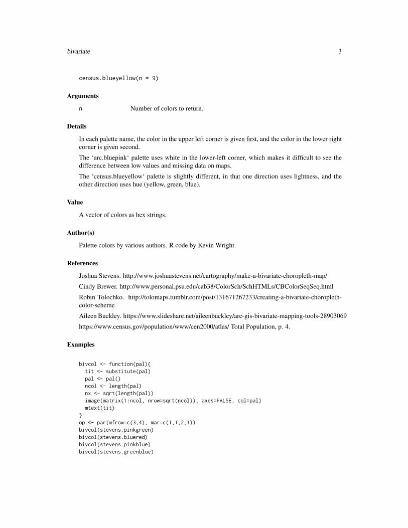
In each palette name, the color in the upper left corner is given first, and the color in the lower rightcorner is given second.

The ‘arc.bluepink‘ palette uses white in the lower-left corner, which makes it difficult to see thedifference between low values and missing data on maps.

The ‘census.blueyellow‘ palette is slightly different, in that one direction uses lightness, and theother direction uses hue (yellow, green, blue).

Value

A vector of colors as hex strings.

Author(s)

Palette colors by various authors. R code by Kevin Wright.

References

Joshua Stevens. http://www.joshuastevens.net/cartography/make-a-bivariate-choropleth-map/

Cindy Brewer. http://www.personal.psu.edu/cab38/ColorSch/SchHTMLs/CBColorSeqSeq.html

Robin Tolochko. http://tolomaps.tumblr.com/post/131671267233/creating-a-bivariate-choropleth-color-scheme

Aileen Buckley. https://www.slideshare.net/aileenbuckley/arc-gis-bivariate-mapping-tools-28903069

https://www.census.gov/population/www/cen2000/atlas/ Total Population, p. 4.

Examples

bivcol <- function(pal){tit <- substitute(pal)pal <- pal()ncol <- length(pal)nx <- sqrt(length(pal))image(matrix(1:ncol, nrow=sqrt(ncol)), axes=FALSE, col=pal)mtext(tit)

}op <- par(mfrow=c(3,4), mar=c(1,1,2,1))bivcol(stevens.pinkgreen)bivcol(stevens.bluered)bivcol(stevens.pinkblue)bivcol(stevens.greenblue)

4 brewer

bivcol(stevens.purplegold)bivcol(brewer.orangeblue)bivcol(brewer.pinkblue)bivcol(tolochko.redblue)bivcol(arc.bluepink)bivcol(census.blueyellow)par(op)

brewer ColorBrewer palettes

Description

These functions provide a unified access to the ColorBrewer palettes.

Usage

brewer.blues(n)

brewer.bugn(n)

brewer.bupu(n)

brewer.gnbu(n)

brewer.greens(n)

brewer.greys(n)

brewer.oranges(n)

brewer.orrd(n)

brewer.pubu(n)

brewer.pubugn(n)

brewer.purd(n)

brewer.purples(n)

brewer.rdpu(n)

brewer.reds(n)

brewer.ylgn(n)

brewer 5

brewer.ylgnbu(n)

brewer.ylorbr(n)

brewer.ylorrd(n)

brewer.brbg(n)

brewer.piyg(n)

brewer.prgn(n)

brewer.puor(n)

brewer.rdbu(n)

brewer.rdgy(n)

brewer.rdylbu(n)

brewer.rdylgn(n)

brewer.spectral(n)

brewer.accent(n)

brewer.dark2(n)

brewer.paired(n)

brewer.pastel1(n)

brewer.pastel2(n)

brewer.set1(n)

brewer.set2(n)

brewer.set3(n)

Arguments

n The number of colors to display for palette functions.

Details

The palette names begin with ’brewer’ to make it easier to use auto-completion.

6 brewer

Value

A vector of colors.

Examples

# Sequentialpal.bands(brewer.blues, brewer.bugn, brewer.bupu, brewer.gnbu, brewer.greens,

brewer.greys, brewer.oranges, brewer.orrd, brewer.pubu, brewer.pubugn,brewer.purd, brewer.purples, brewer.rdpu, brewer.reds, brewer.ylgn,brewer.ylgnbu, brewer.ylorbr, brewer.ylorrd)

# Divergingpal.bands(brewer.brbg, brewer.piyg, brewer.prgn, brewer.puor, brewer.rdbu,

brewer.rdgy, brewer.rdylbu, brewer.rdylgn, brewer.spectral)

# Qualtitativepal.bands(brewer.accent(8), brewer.dark2(8), brewer.paired(12), brewer.pastel1(9),

brewer.pastel2(8), brewer.set1(9), brewer.set2(8), brewer.set3(10),labels=c("brewer.accent", "brewer.dark2", "brewer.paired", "brewer.pastel1","brewer.pastel2", "brewer.set1", "brewer.set2", "brewer.set3"))

## Not run:

# Sequentialpal.test(brewer.blues)pal.test(brewer.bugn)pal.test(brewer.bupu)pal.test(brewer.gnbu)pal.test(brewer.greens)pal.test(brewer.greys)pal.test(brewer.oranges)pal.test(brewer.orrd)pal.test(brewer.pubu) # goodpal.test(brewer.pubugn) # goodpal.test(brewer.purd)pal.test(brewer.purples)pal.test(brewer.rdpu)pal.test(brewer.reds)pal.test(brewer.ylgn)pal.test(brewer.ylgnbu)pal.test(brewer.ylorbr)pal.test(brewer.ylorrd)

# Diverging, max n=11 colorspal.test(brewer.brbg)pal.test(brewer.piyg)pal.test(brewer.prgn)pal.test(brewer.puor)pal.test(brewer.rdbu)pal.test(brewer.rdgy)pal.test(brewer.rdylbu)

continuous 7

pal.test(brewer.rdylgn)pal.test(brewer.spectral)

# Qualtitative. These are weird...don't do thispal.test(brewer.accent)pal.test(brewer.dark2)pal.test(brewer.paired)pal.test(brewer.pastel1)pal.test(brewer.pastel2)pal.test(brewer.set1)pal.test(brewer.set2)pal.test(brewer.set3)

# Need to move these to 'tests'pal.bands(brewer.accent(3), brewer.accent(4), brewer.accent(5), brewer.accent(6),

brewer.accent(7), brewer.accent(8), brewer.accent(9), brewer.accent(10),brewer.accent(11), brewer.accent(12))

#brewer.purd(1) # Should err#brewer.purd(2) # Should errbrewer.purd(3)brewer.purd(9)brewer.purd(25)pal.bands(brewer.purd(3), brewer.purd(4), brewer.purd(5), brewer.purd(6),

brewer.purd(7), brewer.purd(8), brewer.purd(9), brewer.purd(10),brewer.purd(11), brewer.purd(12), brewer.purd(13), brewer.purd(14),brewer.purd(15), brewer.purd(100))

## End(Not run)

continuous Miscellaneous colormaps

Description

Colormaps designed for continuous data.

Usage

cubehelix(n = 25, start = 0.5, r = -1.5, hue = 1, gamma = 1)

gnuplot(n = 25, trim = 0.1)

tol.rainbow(n = 25, manual = TRUE)

jet(n)

parula(n)

8 continuous

coolwarm(n)

warmcool(n)

cividis(n)

Arguments


start Start angle (radians) of the helix

r Number of rotations of the helix

hue Saturation of the colors, 0 = grayscale, 1 = fully saturated

gamma gamma < 1 emphasizes low intensity values, gamma > 1 emphasizes high inten-sity values

trim Proportion of tail colors to trim, default 0.1

manual If TRUE, return manually-calibrated colors.

Details

The coolwarm and ’warmcool’ palette by Moreland (2009) is colorblind safe. The transition to andfrom gray is smooth, to reduce Mach banding.

The cubehelix palette is sometimes used in astronomy. Images using this palette will look mono-tonically increasing to both the human eye and when printed in black and white. This palette isnamed ’cubehelix’ because the r,g,b values produced can be visualised as a squashed helix aroundthe diagonal from black (0,0,0) to white (1,1,1) in the r,g,b color cube.

The gnuplot palette uses black-blue-pink-yellow colors. This palette looks good when printed inblack and white. Identical to the sp::bpy.colors palette.

The jet palette should not be used and is only provided for historical interest. The code for thispalette comes from the example section of colorRampPalette. The ’jet’ palette gained popularityas the default colormap in older versions of Matlab. Because of the unevenness of the gradient, jetwill exaggerate some features of the data and minimize other features.

The parula palette here is similar to the default Matlab palette. Specific colors were adapted fromthe BIDS/colormap package.

The tol.rainbow palette by Tol (2012) is a dark rainbow palette from purple to red which worksmuch better than standard rainbow palettes for colorblind people. If 1 <= n <= 13, manually-chosenequidistant rainbow colors are used, where distances are defined by the CIEDE2000 color differ-ence. If 14 <= n <= 21, manually-chosen triplets of colours are used. If n > 21 or if manual=FALSE,the palette computes the colors according to Equation 3 of Tol (2012).

The cividis palette by Jamie R. Nuñez, Christopher R. Anderton, Ryan S. Renslow, is a variationof viridis that is less colorful.

Value

A vector of colors.

continuous 9

Author(s)


References

Dave A. Green. (2011). A colour scheme for the display of astronomical intensity images. Bull.Astr. Soc. India, 39, 289-295. http://arxiv.org/abs/1108.5083 http://www.mrao.cam.ac.uk/~dag/CUBEHELIX/

Kenneth Moreland. (2009). Diverging Color Maps for Scientific Visualization. Proceedings of the5th International Symposium on Visual Computing. http://www.kennethmoreland.com/color-maps/http://dx.doi.org/10.1007/978-3-642-10520-3_9

Paul Tol (2012). Color Schemes. SRON technical note, SRON/EPS/TN/09-002. https://personal.sron.nl/~pault/

My Favorite Colormap. (gnuplot) https://web.archive.org/web/20040119000943/http://www.ihe.uni-karlsruhe.de/mitarbeiter/vonhagen/palette.en.html

MathWorks documentation. http://www.mathworks.com/help/matlab/ref/colormap.html

BIDS/colormap. https://github.com/BIDS/colormap/blob/master/parula.py

Jamie R. Nuñez, Christopher R. Anderton, Ryan S. Renslow (2017). An optimized colormap forthe scientific community. https://arxiv.org/abs/1712.01662

Examples

pal.bands(coolwarm, cubehelix, gnuplot, jet, parula, tol.rainbow, cividis)

if(FALSE){

# ----- coolwarm -----pal.test(coolwarm) # Minimal mach banding# Note the mach banding gray line in the following:# pal.volcano(colorRampPalette(c("#3B4CC0", "lightgray", "#B40426")))

# ----- cubehelix -----# Full range of colors. Pink is overwhelming. Not the best choice.pal.test(cubehelix)

# Mostly blues/greens. Dark areas severely too black.# Similar, but more saturated. See: http://inversed.ru/Blog_2.htmpal.volcano(function(n) cubehelix(n, start=.25, r=-.67, hue=1.5))

# Dark colors totally lose structure of the volcano peak.op <- par(mfrow=c(2,2), mar=c(2,2,2,2))image(volcano, col = cubehelix(51), asp = 1, axes=0, main="cubehelix")image(volcano, col = cubehelix(51, start=.25, r=-.67, hue=1.5), asp = 1, axes=0, main="cubehelix")image(volcano, col = rev(cubehelix(51)), asp = 1, axes=0, main="cubehelix")image(volcano, col = rev(cubehelix(51, start=.25, r=-.67, hue=1.5)),

asp = 1, axes=0, main="cubehelix")par(op)

# ----- gnuplot -----pal.test(gnuplot)

10 discrete

# ----- jet -----# pal.volcano(jet)pal.test(jet)

# ----- parula -----# pal.volcano(parula)pal.test(parula)

# ----- tol.rainbow -----# pal.volcano(tol.rainbow)pal.test(tol.rainbow)

}

# ----- cividis -----# pal.volcano(cividis)pal.test(cividis)

discrete Discrete palettes

Description

Color palettes designed for discrete, categorical data with a small number of categories.

Usage

alphabet(n = 26)

alphabet2(n = 26)

cols25(n = 25)

glasbey(n = 32)

kelly(n = 22)

polychrome(n = 36)

stepped(n = 24)

tableau20(n = 20)

tol(n = 12)

watlington(n = 16)

discrete 11

Arguments


Details

The alphabet palette has 26 distinguishable colors that have logical names starting with the Englishalphabet letters A, B, ... Z. This palette is based on the work by Green-Armytage (2010), but usesthe names ’orange’ instead of ’orpiment’, and ’magenta’ instead of ’mallow’.

The alphabet2 palette uses a similar idea with slightly different colors and slightly different names.This palette comes from the Polychrome package, generated with the createPalette function andthen manually arranged and named.

The cols25 palette was created experimentally by Wright (unpublished) to create a set of colorsthat are distinct.

The glasbey palette by Glasbey et al (2007) has 32 colors that are maximally distinct. Glasbey has’white’ as the second color, but in this version of the palette, the color ’white’ is moved to the end,and is actually light-gray, #F2F3F4.

The kelly palette of 22 colors maximize the contrast between colors in a set if the colors arechosen in sequential order. Kelly paid attention to the needs of people with color blindness. Thefirst nine colors work well for such people and people with normal vision. Kelly did not provideRGB color values, and the paper was in black-and-white. A color image of the Kelly palette canbe found in Green-Armytage (2010). The color ’white’ has been re-defined as light-gray, #F2F3F4.Commentary: We think the kelly palette has an over-abundance of orange-ish colors, the purplesare not very distinct, color 22 (olive green) is almost identical to color 2 (black), etc.

The polychrome palette is also from the Polychrome package. Colors were given a name from theISCC-NBS standard.

The stepped palette has 24 colors (5 hues, 4 levels within each hue, plus 4 shades of gray) that isuseful for showing varying levels within categories. Inspired by (http://geog.uoregon.edu/datagraphics/color_scales.htm),but in order to better separate these colors in RGB space, red hue 0 was moved to hue 350, greenhue 80 moved to hue 90. The number of colors within each hue was reduced from 5 to 4, and grayshades were added.

The tableau20 palette has 10 pairs of dark/light colors that are used by the Tableau software.

The tol palette has 12 colors by Paul Tol.

The watlington palette has 16 colors. The color ’white’ has been re-defined as light-gray, #F2F3F4.

Value

A vector of colors as hex strings.

Author(s)


12 discrete

References

Robert M. Boynton. (1989) Eleven Colors That Are Almost Never Confused. Proc. SPIE 1077,Human Vision, Visual Processing, and Digital Display, 322-332. http://doi.org/10.1117/12.952730

Kevin R. Coombes (2016). Polychrome. https://rdrr.io/rforge/Polychrome/man/alphabet.html

Chris Glasbey, Gerie van der Heijden, Vivian F. K. Toh, Alision Gray (2007). Colour Displays forCategorical Images. Color Research and Application, 32, 304-309. http://doi.org/10.1002/col.20327

P. Green-Armytage (2010): A Colour Alphabet and the Limits of Colour Coding. Colour: Design& Creativity (5) (2010): 10, 1-23. www.aic-color.org/journal/v5/jaic_v5_06.pdf

K. Kelly (1965): Twenty-two colors of maximum contrast. Color Eng., 3(6), 1965. http://www.iscc.org/pdf/PC54_1724_001.pdf

Paul Tol (2012). Color Schemes. SRON technical note, SRON/EPS/TN/09-002. https://personal.sron.nl/~pault/

John Watlington. An Optimum 16 Color Palette. http://alumni.media.mit.edu/~wad/color/palette.html

Color Schemes Appropriate for Scientific Data Graphics http://geog.uoregon.edu/datagraphics/color_scales.htm

Examples

pal.bands(alphabet, alphabet2, cols25, glasbey, kelly, polychrome,stepped, tableau20, tol, watlington)

## Not run:alphabet()alphabet()["jade"]pal.bands(alphabet,n=26)pal.heatmap(alphabet)# pal.cube(alphabet)

pal.heatmap(alphabet2)

pal.heatmap(cols25)

pal.heatmap(glasbey(32))# pal.cube(glasbey, n=32) # Blues are close together

pal.heatmap(kelly(22)) # too many orange/pink colors

pal.heatmap(polychrome)

pal.heatmap(stepped, n=24)

pal.heatmap(tol, 12)

pal.heatmap(watlington(16))

## End(Not run)

kovesi 13

kovesi Peter Kovesi’s perceptually uniform colormaps

Description

Peter Kovesi’s perceptually uniform colormaps

Usage

kovesi.cyclic_grey_15_85_c0(n)

kovesi.cyclic_grey_15_85_c0_s25(n)

kovesi.cyclic_mrybm_35_75_c68(n)

kovesi.cyclic_mrybm_35_75_c68_s25(n)

kovesi.cyclic_mygbm_30_95_c78(n)

kovesi.cyclic_mygbm_30_95_c78_s25(n)

kovesi.cyclic_wrwbw_40_90_c42(n)

kovesi.cyclic_wrwbw_40_90_c42_s25(n)

kovesi.diverging_isoluminant_cjm_75_c23(n)

kovesi.diverging_isoluminant_cjm_75_c24(n)

kovesi.diverging_isoluminant_cjo_70_c25(n)

kovesi.diverging_linear_bjr_30_55_c53(n)

kovesi.diverging_linear_bjy_30_90_c45(n)

kovesi.diverging_rainbow_bgymr_45_85_c67(n)

kovesi.diverging_bkr_55_10_c35(n)

kovesi.diverging_bky_60_10_c30(n)

kovesi.diverging_bwr_40_95_c42(n)

kovesi.diverging_bwr_55_98_c37(n)

kovesi.diverging_cwm_80_100_c22(n)

14 kovesi

kovesi.diverging_gkr_60_10_c40(n)

kovesi.diverging_gwr_55_95_c38(n)

kovesi.diverging_gwv_55_95_c39(n)

kovesi.isoluminant_cgo_70_c39(n)

kovesi.isoluminant_cgo_80_c38(n)

kovesi.isoluminant_cm_70_c39(n)

kovesi.linear_bgy_10_95_c74(n)

kovesi.linear_bgyw_15_100_c67(n)

kovesi.linear_bgyw_15_100_c68(n)

kovesi.linear_blue_5_95_c73(n)

kovesi.linear_blue_95_50_c20(n)

kovesi.linear_bmw_5_95_c86(n)

kovesi.linear_bmw_5_95_c89(n)

kovesi.linear_bmy_10_95_c71(n)

kovesi.linear_bmy_10_95_c78(n)

kovesi.linear_gow_60_85_c27(n)

kovesi.linear_gow_65_90_c35(n)

kovesi.linear_green_5_95_c69(n)

kovesi.linear_grey_0_100_c0(n)

kovesi.linear_grey_10_95_c0(n)

kovesi.linear_kry_5_95_c72(n)

kovesi.linear_kry_5_98_c75(n)

kovesi.linear_kryw_5_100_c64(n)

kovesi.linear_kryw_5_100_c67(n)

kovesi 15

kovesi.linear_ternary_blue_0_44_c57(n)

kovesi.linear_ternary_green_0_46_c42(n)

kovesi.linear_ternary_red_0_50_c52(n)

kovesi.rainbow_bgyr_35_85_c72(n)

kovesi.rainbow(n)

kovesi.rainbow_bgyr_35_85_c73(n)

kovesi.rainbow_bgyrm_35_85_c69(n)

kovesi.rainbow_bgyrm_35_85_c71(n)

Arguments


Details

All colormaps are named using Peter Kovesi’s naming scheme: <category>_<huesequence>_<lightnessrange>_c<meanchroma>_s<colorshift>

Note: kovesi.rainbow is another name for rainbow_bgyr_35_85_c72.

Value

A vector of colors.

Author(s)

Colormaps by Peter Kovesi. R code by Kevin Wright.

References

Peter Kovesi (2016). CET Perceptually Uniform Colour Maps. http://peterkovesi.com/projects/colourmaps/

Peter Kovesi (2015). Good Colour Maps: How to Design Them. Arxiv. https://arxiv.org/abs/1509.03700

https://bokeh.github.io/colorcet/

Examples

if(FALSE){pal.bands(kovesi.cyclic_grey_15_85_c0, kovesi.cyclic_grey_15_85_c0_s25,kovesi.cyclic_mrybm_35_75_c68, kovesi.cyclic_mrybm_35_75_c68_s25,kovesi.cyclic_mygbm_30_95_c78, kovesi.cyclic_mygbm_30_95_c78_s25,kovesi.cyclic_wrwbw_40_90_c42, kovesi.cyclic_wrwbw_40_90_c42_s25,kovesi.diverging_isoluminant_cjm_75_c23, kovesi.diverging_isoluminant_cjm_75_c24,kovesi.diverging_isoluminant_cjo_70_c25, kovesi.diverging_linear_bjr_30_55_c53,kovesi.diverging_linear_bjy_30_90_c45, kovesi.diverging_rainbow_bgymr_45_85_c67,

16 matplotlib

kovesi.diverging_bkr_55_10_c35, kovesi.diverging_bky_60_10_c30,kovesi.diverging_bwr_40_95_c42, kovesi.diverging_bwr_55_98_c37,kovesi.diverging_cwm_80_100_c22, kovesi.diverging_gkr_60_10_c40,kovesi.diverging_gwr_55_95_c38, kovesi.diverging_gwv_55_95_c39,kovesi.isoluminant_cgo_70_c39, kovesi.isoluminant_cgo_80_c38,kovesi.isoluminant_cm_70_c39, kovesi.linear_bgy_10_95_c74,kovesi.linear_bgyw_15_100_c67, kovesi.linear_bgyw_15_100_c68,kovesi.linear_blue_5_95_c73, kovesi.linear_blue_95_50_c20,kovesi.linear_bmw_5_95_c86, kovesi.linear_bmw_5_95_c89,kovesi.linear_bmy_10_95_c71, kovesi.linear_bmy_10_95_c78,kovesi.linear_gow_60_85_c27, kovesi.linear_gow_65_90_c35,kovesi.linear_green_5_95_c69, kovesi.linear_grey_0_100_c0,kovesi.linear_grey_10_95_c0, kovesi.linear_kry_5_95_c72,kovesi.linear_kry_5_98_c75, kovesi.linear_kryw_5_100_c64,kovesi.linear_kryw_5_100_c67, kovesi.linear_ternary_blue_0_44_c57,kovesi.linear_ternary_green_0_46_c42, kovesi.linear_ternary_red_0_50_c52,kovesi.rainbow_bgyr_35_85_c72, kovesi.rainbow_bgyr_35_85_c73,kovesi.rainbow_bgyrm_35_85_c69, kovesi.rainbow_bgyrm_35_85_c71)}

matplotlib Matplotlib colormaps

Description

Viridis family of colormaps as found in Matplotlib. Designed to be perceptually uniform, but gen-erally too dark to be useful.

Usage

magma(n)

inferno(n)

plasma(n)

viridis(n)

Arguments

n Number of colors to return

Value

A vector of colors

Author(s)

Palettes by Matteo Niccoli. R code by Kevin Wright.

niccoli 17

Examples

pal.bands(magma, inferno, plasma, viridis)

niccoli Matteo Niccoli’s perceptually uniform colormaps

Description

These colormaps are intended by be more perceptually balanced than traditional rainbow-like palettes.

Usage

cubicyf(n)

isol(n)

cubicl(n)

linearl(n)

linearlhot(n)

Arguments

n Number of colors to return

Details

isol(): Lab-based isoluminant rainbow with constant luminance L*=60. Best choice for display-ing interval data with external lighting. best for displaying interval data with external lighting. Thisis so as to allow the lighting to provide the shading to highlight the details of interest. If lightingis combined with a colormap that has its own luminance function associated - even as simple as alinear increase this will confuse the viewer.

linearl(): Lab-based linear lightness rainbow. A linear lightness modification of Matlab’s ’hot’palette. For interval data displayed without external lighting. 100

linlhot(): Linear lightness modification of Matlab’s hot color palette. For interval data displayedwithout external lighting 100

cubicyf(): Lab-based rainbow scheme with cubic-law luminance(default) For interval data dis-played without external lighting 100

cubicl(): Lab-based rainbow scheme with cubic-law luminance For interval data displayed with-out external lighting Similar to cubicyf(), but has red at high end (a modest deviation from 100

Value

A vector of colors

18 ocean

Author(s)

Palettes by Matteo Niccoli. R code by Kevin Wright.

References

Matteo Niccoli (2010). Perceptually improved colormaps. http://www.mathworks.com/matlabcentral/fileexchange/28982-perceptually-improved-colormaps Color definitions from here: http://www.mathworks.com/matlabcentral/fileexchange/28982-perceptually-improved-colormaps/content/pmkmp/pmkmp.m https://mycarta.wordpress.com/2012/05/29/the-rainbow-is-dead-long-live-the-rainbow-series-outline/

Examples

pal.bands(cubicyf,cubicl,isol,linearl,linearlhot)pal.test(cubicyf) # purple blue greenpal.test(cubicl) # purple blue green orange# pal.test(isol) # magenta blue green red. Poor in green area.# pal.test(linearl) # black blue green tan. Poor in black area.# pal.test(linearlhot) # black red yellow

ocean Oceanography perceptually uniform colormaps

Description

These palettes have been designed to be a collection of perceptually uniform colormaps designedfor oceanographic data display.

Usage

ocean.algae(n)

ocean.deep(n)

ocean.dense(n)

ocean.gray(n)

ocean.haline(n)

ocean.ice(n)

ocean.matter(n)

ocean.oxy(n)

ocean.phase(n)

ocean 19

ocean.solar(n)

ocean.thermal(n)

ocean.turbid(n)

ocean.balance(n)

ocean.curl(n)

ocean.delta(n)

ocean.amp(n)

ocean.speed(n)

ocean.tempo(n)

Arguments

n Number of colors

Details

The ’oxy’ palette does not include gray as shown in Thyng (2016).

The ’balance’, ’delta’, and ’curl’ palettes were originally given as 2*256 colors (256 each for theleft and right half of the palette) and have been downsampled to 256 colors.

The palettes from matplotlib have been converted from RGB codes to hexadecimal strings for usein this package.

Value

None

Author(s)

Palette colors by Kristen Thyng. R code by Kevin Wright

References

Thyng, K.M., C.A. Greene, R.D. Hetland, H.M. Zimmerle, and S.F. DiMarco (2016). True colors ofoceanography: Guidelines for effective and accurate colormap selection. Oceanography, 29(3):9-13, http://dx.doi.org/10.5670/oceanog.2016.66.

Examples

pal.bands(ocean.thermal, ocean.haline, ocean.solar, ocean.ice, ocean.gray,

20 pal.bands

ocean.oxy, ocean.deep, ocean.dense, ocean.algae, ocean.matter,ocean.turbid, ocean.speed, ocean.amp, ocean.tempo, ocean.phase,ocean.balance, ocean.delta, ocean.curl, main="Ocean palettes")

## Not run:pal.test(ocean.thermal)pal.test(ocean.haline) # better than parula!pal.test(ocean.solar)pal.test(ocean.ice)pal.test(ocean.gray)pal.test(ocean.oxy)pal.test(ocean.deep)pal.test(ocean.dense)pal.test(ocean.algae)pal.test(ocean.matter)pal.test(ocean.turbid)pal.test(ocean.speed)pal.test(ocean.amp)pal.test(ocean.tempo)pal.test(ocean.phase)pal.test(ocean.balance)pal.test(ocean.delta)pal.test(ocean.curl)

## End(Not run)

pal.bands Show palettes and colormaps as colored bands

Description

Show palettes as colored bands.

Usage

pal.bands(..., n = 100, labels = NULL, main = NULL, gap = 0.1,sort = "none", show.names = TRUE)

Arguments

... Palettes/colormaps, each of which is either (1) a vectors of colors or (2) a func-tion returning a vector of colors.


labels Labels for palettes

main Title at top of page.

gap Vertical gap between bars, default is 0.1

pal.channels 21

sort If sort="none", palettes are not sorted. If sort="hue", palettes are sorted by hue.If sort="luminance", palettes are sorted by luminance.

show.names If TRUE, show color names

Details

What to look for:

1. A good discrete palette has distinct colors.

2. A good continuous colormap does not show boundaries between colors. For example, therainbow() palette is poor, showing bright lines at yellow, cyan, pink.

Examples

pal.bands(c('red','white','blue'), rainbow)

op=par(mar=c(0,5,3,1))pal.bands(cubehelix, gnuplot, jet, tol.rainbow, inferno,

magma, plasma, viridis, parula, n=200, gap=.05)par(op)

# Examples of sortinglabs=c('alphabet','alphabet2', 'glasbey','kelly','polychrome', 'watlington')op=par(mar=c(0,5,3,1))pal.bands(alphabet(), alphabet2(), glasbey(), kelly(),

polychrome(), watlington(), sort="hue",labels=labs, main="sorted by hue")

par(op)pal.bands(alphabet(), alphabet2(), glasbey(), kelly(),

polychrome(), watlington(), sort="luminance",labels=labs, main="sorted by luminance")

pal.channels Show the red, green, blue, gray amount in colors of a palette

Description

The amount of red, green, blue, and gray in colors are shown.

Usage

pal.channels(pal, n = 150, main = "")

Arguments

pal A palette function or a vector of colors.


main Main title.

22 pal.cluster

Details

What to look for:

1. Sequential data should usually be shown with a colormap that is smoothly increasing in lightness,as shown by the gray line.

Value

None

Author(s)

Kevin Wright

References

None

Examples

pal.channels(parula)pal.channels(coolwarm)# pal.channels(glasbey) # Nonsensical.

pal.cluster Show a palette with hierarchical clustering

Description

The palette colors are converted to LUV coordinates before clustering. (RGB coordinates are avail-able, but not recommended.)

Usage

pal.cluster(pal, n = 50, type = "LUV", main = "")

Arguments



type Either "LUV" (default) or "RGB".

main Title to display at the top of the test image

Details

What to look for:

Colors that are visually similar tend to be clustered together.

pal.compress 23

Value

None

Author(s)

Kevin Wright

References

None

Examples

pal.cluster(alphabet(), main="alphabet")pal.cluster(glasbey, main="glasbey") # two royal blues are very similarpal.cluster(kelly, main="kelly") # two black-ish colors are very similar# pal.cluster(watlington, main="watlington")# pal.cluster(coolwarm(15), main="coolwarm") # curiously, grey clusters with blue

pal.compress Compress a colormap function to fewer colors

Description

Compress a colormap function to fewer colors

Usage

pal.compress(pal, n = 5, thresh = 2.5)

Arguments

pal A colormap function or a vector of colors.

n Initial number of colors to use.

thresh Maximum allowable Lab distance from original palette

Details

Colormap functions are often defined with many more colors than needed. This function compressesa colormap function down to a sample of colors that can be passed into ’colorRampPalette’ and re-create the original palette with a just-noticeable-difference.

Colormaps that are defined as a smoothly varying ramp between a set of colors often compress quitewell. Colormaps that are defined by functions may not compress well.

Value

A vector of colors

24 pal.csf

Author(s)

Kevin Wright

References

None.

Examples

# The 'cm.colors' palette in R compresses to only 3 colorscm2 <- pal.compress(cm.colors, n=3)pal.bands(cm.colors(255), colorRampPalette(cm2)(255), cm2,labels=c('original','compressed','basis'), main="cm.colors")

# The 'heat.colors' palette needs 84 colorsheat2 <- pal.compress(heat.colors, n=3)pal.bands(heat.colors(255), colorRampPalette(heat2)(255), heat2,labels=c('original','compressed','basis'), main="heat.colors")

# The 'topo.colors' palette needs 249 colors because of the discontinuity# topo2 <- pal.compress(topo.colors, n=3)# pal.bands(topo.colors(255), colorRampPalette(topo2)(255), topo2,# labels=c('original','compressed','basis'), main="topo.colors")

# smooth palettes usually easy to compressp1 <- coolwarm(255)cool2 <- pal.compress(coolwarm)p2 <- colorRampPalette(cool2)(255)pal.bands(p1, p2, cool2,labels=c('original','compressed', 'basis'), main="coolwarm")pal.maxdist(p1,p2) # 2.33

pal.csf Show a colormap with a Campbell-Robson Contrast Sensitivity Chart

Description

In a contrast sensitivity figure as drawn by this function, the spatial frequency increases from leftto right and the contrast decreases from bottom to top. The bars in the figure appear taller in themiddle of the image than at the edges, creating an upside-down "U" shape, which is the "contrastsensitivity function". Your perception of this curve depends on the viewing distance.

Usage

pal.csf(pal, n = 150, main = "")

pal.cube 25

Arguments

pal A continuous colormap function


main Main title.

Details

What to look for:

1. Are the vertical bands visible across the full vertical axis?

2. Do the vertical bands blur together?

Value

None

Author(s)

Kevin Wright

References

Izumi Ohzawa. Make Your Own Campbell-Robson Contrast Sensitivity Chart. http://ohzawa-lab.bpe.es.osaka-u.ac.jp/ohzawa-lab/izumi/CSF/A_JG_RobsonCSFchart.html

Campbell, F. W. and Robson, J. G. (1968). Application of Fourier analysis to the visibility ofgratings. Journal of Physiology, 197: 551-566.

Examples

pal.csf(brewer.greys) # Classic example from psychologypal.csf(parula)

pal.cube Show one palette/colormap in three dimensional RGB or LUV space

Description

The palette is converted to RGB or LUV coordinates and plotted in a three-dimensional scatterplot.The LUV space is probably better, but it is easier to tweak colors by hand in RGB space.

Usage

pal.cube(pal, n = 100, label = FALSE, type = "RGB")

26 pal.dist

Arguments

pal A palette/colormap function or a vector of colors.


label If TRUE, show color name/value on plot

type Either "RGB" (default) or "LUV".

Details

What to look for:

A good palette has colors that are spread somewhat uniformly in 3D.

Value

None

References

None

Examples

## Not run:pal.cube(cubehelix)pal.cube(glasbey, n=32) # RGB, blues are too close to each otherpal.cube(glasbey, n=32, type="LUV")pal.cube(cols25(25), type="LUV", label=TRUE)# To open a second cubergl.open() # Open a new RGL devicergl.bg(color = "white") # Setup the background colorpal.cube(colors()[c(1:152, 254:260, 362:657)]) # All R non-grey colors

## End(Not run)

pal.dist Measure the pointwise distance between two palettes

Description

Measure the pointwise distance between two palettes

Usage

pal.dist(pal1, pal2, n = 255)

pal.heatmap 27

Arguments

pal1 A color palette (function or vector)


n Number of colors to use, default 255

Details

The distance between two palettes (of equal length) is calculated pointwise using the Lab colorspace. A ’just noticeable difference’ between colors is roughly 2.3.

Value

A vector of n distances.

Author(s)

Kevin Wright

References

https://en.wikipedia.org/wiki/Color_difference

Examples

pa0 <- c("#ff0000","#00ff00","#0000ff")pa1 <- c("#fa0000","#00fa00","#0000fa") # 2.4pa2 <- c("#f40000","#00f400","#0000f4") # 5.2pal.dist(pa0,pa1) # 1.87, 2.36, 2.11pal.dist(pa0,pa2) # 4.12 5.20 4.68pal.bands(pa1,pa0,pa2, labels=c("1.87 2.36 2.11","0","4.12 5.20 4.68"))title("Lab distances from middle palette")

pal.heatmap Show a palette/colormap with a heatmap

Description

Show a palette/colormap with a heatmap

Usage

pal.heatmap(pal, n = 25, miss = 0.05, main = "")

28 pal.map

Arguments


n The number of squares vertically in the heatmap.

miss Fraction of squares with missing values, default .05.

main Main title

Value

None.

Author(s)

Kevin Wright

References

None

Examples

pal.heatmap(brewer.paired, n=12)pal.heatmap(coolwarm, n=12)pal.heatmap(tol, n=12)pal.heatmap(glasbey, n=32)pal.heatmap(kelly, n=22, main="kelly", miss=.25)

pal.map Show a palette using a map of U.S. counties

Description

What to look for:

Usage

pal.map(pal = brewer.paired, n = 12, main = "")

Arguments



main Main title

pal.map 29

Details

1. Are regions distinct?

2. Are outliers within each region distinct?

Display a palette on a choropleth map similar to ColorBrewer.

Broad bands of color are easy to distinguish. Does the palette allow visibility of outlier counties inthe larger regions? Does the palette allow identification of colors when the pattern is more complex(as in the lower left corner of the map)?

Notes. The map shown by the ColorBrewer website is an SVG here https://github.com/axismaps/colorbrewer/tree/master/map/map.svgwhich contains the class identifier for each polygon, for 3 to 12 classes. Unfortunately, the poly-gons have no other identification (e.g. FIPS, county name). We used the identify.map function inR to manually define the classes similar to the 12-class map of ColorBrewer. This proved to betoo tedious to do more than once, so our maps of 1-11 classes were created by combining classesfrom the 12-class map. The ColorBrewer website sometimes used this strategy to combine classes,but not always. The ’outlier’ counties and ’random region’ in this version are very similar to the12-region map of ColorBrewer, but there are a few differences, mostly intentional. Also, the mapprojection used here is different from ColorBrewer.

Value

None

Author(s)

Kevin Wright

References

http://www.personal.psu.edu/cab38/Pub_scans/Brewer_pubs.html Map based on www.ColorBrewer.org,by Cynthia A. Brewer, Penn State.

Examples

pal.map(brewer.paired, main="brewer.paired")pal.map(parula)

## Not run:for(i in 3:12){

pal.map(n=i, main=i)}

## End(Not run)

30 pal.maxdist

pal.maxdist Measure the maximum distance between two palettes

Description

Measure the maximum distance between two palettes

Usage

pal.maxdist(pal1, pal2, n = 255)

Arguments



n Number of colors to use, default 255

Details

The distance between two palettes (of equal length) is calculated pointwise using the Lab colorspace. A ’just noticeable difference’ between colors is roughly 2.3.

Value

Numeric value of the maximum distance.

Author(s)

Kevin Wright

References

https://en.wikipedia.org/wiki/Color_difference

Examples

pa0 <- c("#ff0000","#00ff00","#0000ff")pa1 <- c("#fa0000","#00fa00","#0000fa") # 2.4pa2 <- c("#f40000","#00f400","#0000f4") # 5.2pal.maxdist(pa0,pa1) # 2.36pal.maxdist(pa0,pa2) # 5.20pal.bands(pa1,pa0,pa2, labels=c("2.36","0","5.20"))title("Maximum Lab distance from middle palette")

# distance between colormap functionspal.maxdist(coolwarm,warmcool)

pal.safe 31

pal.safe Show a palette/colormap for black/white and colorblind safety

Description

A single palette/colormap is shown (1) without any modifications (2) in black-and-white as if pho-tocopied (3) as seen by deutan color-blind (4) as seen by protan color-blind (5) as seen by tritancolor-blind

Usage

pal.safe(pal, n = 100, main = NULL)

Arguments

pal A palette function or a vector of colors.n The number of colors to display for palette functions.main Title to display at the top of the test image

Details

Rates of colorblindness in women are low, but in men the rates are around 3 to 7 percent, dependingon the race.

What to look for:

1. Are colors still unique when viewed in less-than full color?

2. Is a sequential colormap still sequential?

Value

None.

Author(s)

Kevin Wright

References

Vischeck. http://www.vischeck.com/vischeck/

None

Examples

pal.safe(glasbey)pal.safe(rainbow, main="rainbow") # Really, really badpal.safe(cubicyf(100), main="cubicyf")pal.safe(parula, main="parula")

http://www.vischeck.com/vischeck/

32 pal.scatter

pal.scatter Show a colormap with a scatterplot

Description

What to look for:

Usage

pal.scatter(pal, n = 50, main = "")

Arguments



main Main title

Details

1. Can the colors of each point be uniquely identified?

Value

None.

Author(s)

Kevin Wright

References

None.

Examples

pal.scatter(glasbey, n=31, main="glasbey") # FIXME add legendpal.scatter(parula, n=10) # not a good choice

pal.sineramp 33

pal.sineramp Show a colormap with a sineramp

Description

The test image shows a sine wave superimposed on a ramp of the palette. The amplitude of the sinewave is dampened/modulated from full at the top of the image to 0 at the bottom.

Usage

pal.sineramp(pal, n = 150, nx = 512, ny = 256, amp = 12.5,wavelen = 8, pow = 2, main = "")

Arguments



nx Number of ’pixels’ horizontally (approximate).

ny Number of ’pixels’ vertically

amp Amplitude of sine wave, default 12.5

wavelen Wavelength of sine wave, in pixels, default 8.

pow Power for dampening the sine wave. Default 2. For no dampening, use 0. Forlinear dampening, use 1.

main Main title

Details

The ramp function that the sine wave is superimposed upon is adjusted slightly for each row so thateach row of the image spans the full data range of 0 to 255. The wavelength is chosen to create astimulus that is aligned with the capabilities of human vision. For the default amplitude of 12.5, thetrough to peak distance is 25, which is about 10 percent of the 256 levels of the ramp. Some colorpalettes (like ’jet’) have perceptual flat areas that can hide fluctuations/features of this magnitude.

What to look for:

1. Is the sine wave equally visible horizontally across the entire image?

2. At the bottom, is the ramp smooth, or are there features like vertical bands?

Value

None

Author(s)

Concept by Peter Kovesi. R code by Kevin Wright.

34 pal.test

References

Peter Kovesi (2015). Good Colour Maps: How to Design Them. http://arxiv.org/abs/1509.03700.

Peter Kovesi. A set of perceptually uniform color map files. http://peterkovesi.com/projects/colourmaps/index.html

Peter Kovesi. CET Perceptually Uniform Colour Maps: The Test Image. http://peterkovesi.com/projects/colourmaps/colourmaptestimage.html

Original Julia version by Peter Kovesi from: https://github.com/peterkovesi/PerceptualColourMaps.jl/blob/master/src/utilities.jl

Examples

pal.sineramp(parula)pal.sineramp(jet) # Bad: Indistinct wave in green at top. Mach bands at bottom.pal.sineramp(brewer.greys(100))

pal.test Show a colormap with multiple images

Description

1. Z-curve

Usage

pal.test(pal, main = substitute(pal))

Arguments


main Title to display at the top of the test image

Details

2. Contrast Sensitivity Function.

3. Frequency ramp. See: http://inversed.ru/Blog_2.htm Are the vertical bands visible across the fullvertical axis?

4. 5. Two images of the ’volcano’ elevation data in R using forward/reverse colors. Try to find thehighest point on the volcano peak. Many palettes with dark colors at one end of the palette hide thepeak (e.g. viridis). Also try to decide if the upperleft and upperright corners are the same color.

6. Luminosity in red, green, blue, and grey.

Value

None.

Author(s)

Kevin Wright

pal.volcano 35

References

# See links above.

Examples

pal.test(parula)pal.test(viridis) # dark colors are poorpal.test(coolwarm)

pal.volcano Show a colormap with a surface of volcano elevation

Description

Some palettes with dark colors at one end of the palette hide the shape of the volcano in the darkcolors. Viridis is bad.

Usage

pal.volcano(pal, n = 100, main = "")

Arguments



main Main title

Details

What to look for:

1. Can you locate the highest point on the volcano?

2. Are the upper-right and lower-right corners the same elevation?

3. Do any Mach bands circle the peak?

Value

None.

Examples

pal.volcano(parula)pal.volcano(brewer.rdbu) # Mach banding is badpal.volcano(warmcool, main="warmcool") # No Mach bandpal.volcano(rev(viridis(100))) # Bad: peak position is hidden

36 pal.zcurve

pal.zcurve Show a colormap with a space-filling z-curve

Description

Construct a Z-order curve, coloring cells with a colormap. The difference in color between squaresside-by-side is 1/48 of the full range. The difference in color between one square atop another is1/96 the full range.

Usage

pal.zcurve(pal, n = 64, main = "")

Arguments

pal A continuous color palette function

n Number of squares for the z-curve

main Main title

Details

What to look for:

1. A good color palette of 64 colors should be able to resolve 4 sub-squares within each of the 16squares.

Value

None

Author(s)

Kevin Wright.

References

Peter Karpov. 2016. In Search Of A Perfect Colormap. https://twitter.com/inversed_ru

Z-order curve. https://en.wikipedia.org/wiki/Z-order_curve

Examples

pal.zcurve(parula,n=4,main="parula")pal.zcurve(parula,n=16)pal.zcurve(parula,n=64)pal.zcurve(parula,n=256)

pals 37

pals pals: A package for comprehensive palettes and palette evaluationtools

Description

pals: A package for comprehensive palettes and palette evaluation tools

Details

The terms ’palette’ and ’colormap’ are often interchanged. In this package (1) ’palette’ is usually adiscrete set of distinct colors and (2) ’colormap’ is usually a smoothly varying set of many colors.

The best palette/colormap is determined by (1) the type of structure in the data, (2) the type ofgraphic to be constructed, and (3) the type of device used to show the graphic. The ColorBrewerwebsite approaches this problem by suggesting different colors for qualitative, sequential, and di-verging data, and also considers the display of the graphic on LCD and photocopies. One limitationwith ColorBrewer is that it only uses maps, and does not consider other types of graphics. Forexample, yellow colors work well for polygons (on maps, barcharts, etc), but are poor for lines andscatter plots.

The ’pals’ package provides a suite of tools to evaluate palettes/colormaps.

The design goals of the package are:

• All palettes/colormaps are functions that return a vector of colors.

• The palette function names use only lowercase letters.

• The ’data’ directory is not used.

• Provide an extensive collection of palettes and colormaps.

• Be memory efficient. Colormaps are compressed.

• Provide multiple tools to evaluate palettes.

To learn more, see the vignettes: browseVignettes(package="pals")

penobscot Seismic data horizon offshore of Nova Scotia.

Description

Seismic data offsore of Nova Scotia in Canada. The data have some subtle structures that are inter-esting for comparing colormaps. Full details can be found at https://www.opendtect.org/osr/Main/PENOBSCOT3DSABLEISLANDLicense CC-BY.

Usage

data(penobscot)

38 penobscot

Format

A matrix 463 x 595.

Source

https://github.com/agile-geoscience/notebooks/ https://github.com/agile-geoscience/notebooks/blob/master/Filtering_horizons.ipynb

Examples

#data(penobscot)

# Hall used cubehelix palette# http://wiki.seg.org/wiki/Smoothing_surfaces_and_attributes#External_linksimage(penobscot, col=rev(cubehelix(99)))

# Niccoli suggested LinearL palette# http://wiki.seg.org/wiki/How_to_evaluate_and_compare_color_mapsimage(penobscot, col=linearl(99))

# Use this version to get a colorkey# library(lattice)# levelplot(penobscot, col.regions=rev(cubehelix(99)),# cuts=97, asp=0.7, scale=list(draw=FALSE))

https://github.com/agile-geoscience/notebooks/

https://github.com/agile-geoscience/notebooks/blob/master/Filtering_horizons.ipynb

https://github.com/agile-geoscience/notebooks/blob/master/Filtering_horizons.ipynb

Index

∗Topic datasetspenobscot, 37

alphabet (discrete), 10alphabet2 (discrete), 10arc.bluepink (bivariate), 2

bivariate, 2brewer, 4brewer.orangeblue (bivariate), 2brewer.pinkblue (bivariate), 2

census.blueyellow (bivariate), 2cividis (continuous), 7cols25 (discrete), 10continuous, 7coolwarm (continuous), 7cubehelix (continuous), 7cubicl (niccoli), 17cubicyf (niccoli), 17

discrete, 10

glasbey (discrete), 10gnuplot (continuous), 7

inferno (matplotlib), 16isol (niccoli), 17

jet (continuous), 7

kelly (discrete), 10kovesi, 13

linearl (niccoli), 17linearlhot (niccoli), 17

magma (matplotlib), 16matplotlib, 16

niccoli, 17

ocean, 18

pal.bands, 20pal.channels, 21pal.cluster, 22pal.compress, 23pal.csf, 24pal.cube, 25pal.dist, 26pal.heatmap, 27pal.map, 28pal.maxdist, 30pal.safe, 31pal.scatter, 32pal.sineramp, 33pal.test, 34pal.volcano, 35pal.zcurve, 36pals, 37pals-package (pals), 37parula (continuous), 7penobscot, 37plasma (matplotlib), 16polychrome (discrete), 10

stepped (discrete), 10stevens.bluered (bivariate), 2stevens.greenblue (bivariate), 2stevens.pinkblue (bivariate), 2stevens.pinkgreen (bivariate), 2stevens.purplegold (bivariate), 2

tableau20 (discrete), 10tol (discrete), 10tol.rainbow (continuous), 7tolochko.redblue (bivariate), 2

viridis (matplotlib), 16

warmcool (continuous), 7watlington (discrete), 10

39

Package ‘pals’ - The Comprehensive R Archive Network · Package ‘pals’ January 22, 2018...

Documents

Transcript of Package ‘pals’ - The Comprehensive R Archive Network · Package ‘pals’ January 22, 2018...