Overlapping Ownership, R&D Spillovers, and Antitrust Policy

Ángel L. López Xavier Vives

CESIFO WORKING PAPER NO. 5935 CATEGORY 11: INDUSTRIAL ORGANISATION

ORIGINAL VERSION: JUNE 2016 THIS VERSION: JULY 2018

An electronic version of the paper may be downloaded • from the SSRN website: www.SSRN.com • from the RePEc website: www.RePEc.org

• from the CESifo website: Twww.CESifo-group.org/wp T

ISSN 2364-1428

CESifo Working Paper No. 5935

Overlapping Ownership, R&D Spillovers, and Antitrust Policy

Abstract This paper considers cost-reducing R&D investment with spillovers in a Cournot oligopoly with overlapping ownership. We show that overlapping ownership leads to internalization of rivals. profits by firms and find that, for demand not too convex, increases in overlapping ownership increase (decrease) R&D and output for high (low) enough spillovers while it increases R&D but decreases output for intermediate levels of spillovers. There is scope for overlapping ownership to improve welfare provided that spillovers are sufficiently large. The socially optimal degree of overlapping ownership increases with the number of firms, with the elasticity of demand and of the innovation function, and with the extent of spillover effects. In terms of consumer surplus standard, the desirability of overlapping ownership is greatly reduced even under low market concentration. When R&D has commitment value and spillovers are high the optimal extent of overlapping ownership is higher. The results obtained are robust in the context of a Bertrand oligopoly model with product differentiation.

JEL-Codes: D430, L130, O320.

Keywords: competition policy, partial merger, collusion, innovation, minority shareholdings, common ownership, cross-ownership.

Ángel L. López Departament d’Economia Aplicada

Universitat Autònoma de Barcelona & Public-Private Sector Research Center

IESE Business School / Spain angelluis.lopez@uab.cat

Xavier Vives IESE Business School University of Navarra

Spain - 08034 Barcelona xvives@iese.edu

July 2018 We thank Ramon Faulí-Oller for his insightful initial contributions and to the editor and three anony-mous referees for very useful suggestions. For helpful comments we thank Isabel Busom, Luis Cabral, Guillermo Caruana, Ricardo Flores-Fillol, Matthew Gentzkow, Richard Gilbert, Gerard Llobet, Peter Neary, Volker Nocke, Patrick Rey, Yossi Spiegel, Konrad Stahl, and Javier Suarez, as well as seminar participants at Boston U., IESE, Mannheim, Bologna, CEMFI, PSE, Rovira i Virgili, Stanford and UCLA as well as from participants at numerous workshops and conferences. Orestis Vravosinos provided excellent research assistance. Financial support from the Spanish Ministry of Economy and Competitiveness under ECO2015-63711-P, for López from AGAUR (under SGR 1326) and for Vives from the European Research Council (Advanced Grant No 789013) and AGAUR (under SGR 1244), is gratefully acknowledged.

1 Introduction

In many industries, overlapping ownership arrangements (OOAs) are prevalent in the form

of cross-shareholding agreements among �rms or common ownership by investment funds.1

The latter in particular has grown tremendously in the last three decades and with investors

holding signi�cant stakes in the same industry. The tendency of such OOAs to relax compe-

tition has been documented in the airline and banking industries (Azar et al. forthcoming),

and it has raised antitrust concerns (Elhauge 2016, Baker 2016). At the same time, there

is a debate about whether and why innovative activity and business dynamism have abated

recently (e.g., CEA 2016 and Obama�s executive order to promote competition) pointing at

increased market power as the culprit (e.g., De Loecker and Eeckhout 2017).

The paper contributes by analyzing the interaction of OOAs and R&D activity in the

presence of technological spillovers and deriving testable predictions. OOAs lessen compet-

itive pressure but may have a bene�cial e¤ect on investment provided there are positive

spillovers across �rms. The reason is that OOAs help to internalize the spillover externality,

which is especially important for highly innovative industries.2 Empirical estimates �nd

that gross social returns to R&D are at least twice as high as the private returns (Bloom

et al., 2013). We provide in the paper a welfare analysis that may help elucidate whether

the documented increase in OOAs has outrun its social value and derive competition policy

implications.

In our benchmark model, �rms compete in quantities and invest in cost reduction, and

we consider simultaneous output and R&D decisions. That approach aids tractability while

helping to capture the imperfect observability of �rms�R&D investment levels.3 We con-

sider a general symmetric model of overlapping ownership; this model allows for a range of

corporate control structures (as in Salop and O�Brien 2000) and for distinguishing between

stock acquisitions made by investors and those made by other �rms. The key parameter

is the degree of internalization of rivals�pro�ts (� in our model, ranging from independent

ownership, � = 0, to cartelization � = 1). The parameter � corresponds to what Edgeworth

1A recent example is the car-booking business where apart from cross-ownership (such as Uber and Didi),common investors such as Softbank and Tiger Global hold stakes in Uber, Ola and Grab (see report in theFT by Leslie Hook, September 22, 2017), or such as AFSquare and the mutual fund Fidelity that are alsoinvested in both Uber and Lyft.

2Hansen and Lott (1996) explain how shareholder diversi�cation may help internalize externalities.3Even though R&D investment typically precedes market interaction, this does not mean necessarily that

it has strategic commitment value. R&D investment e¤ort, or even contracts with managers that rewarde¤ort, need not be observable. The evidence on the strategic commitment value of R&D is scant (see Vives2008).

2

(1881) termed the coe¢ cient of �e¤ective sympathy�among individuals. Higher degrees of

overlapping ownership (common or cross-ownership) lead to a higher �. We test the robust-

ness of results by way of a two-stage speci�cation and by considering Bertrand competition

with product di¤erentiation. The latter allows to study the impact of market spillovers on

the e¤ects of changing �. The model subsumes earlier contributions to the literature that

were based on linear or constant elasticity of demand and on speci�c innovation functions.4

Our paper seeks to answer the following questions: How do R&D and output levels vary

with the degree of internalization of rivals�pro�ts? How those relationships are a¤ected by

structural market parameters (demand and cost conditions, industry technological opportu-

nity, and extent of spillovers)? What are the key determinants of the socially optimal extent

of overlapping ownership? How is that optimal level a¤ected by the competition authority�s

objective (to maximize total or rather consumer surplus)?

The main results on the e¤ects of changes in � can be summarized as follows. If demand

is not too convex, then increasing � will increase (resp. decrease) both R&D and output

when spillovers are high (resp. low); for intermediate levels of spillovers, an increase in � will

increase R&D but reduce output. Furthermore, the two thresholds that partition the three

regions for spillovers are generally increasing in the level of market concentration, indicating

that positive R&D and output e¤ects of overlapping ownership should be found typically

only in markets not too concentrated for given spillover levels.

We identify the degree of market concentration and the extent of spillovers as key deter-

minants of the welfare-optimal degree of internalization � be it according to total surplus

(TS) or a consumer surplus (CS) standard. High spillovers increase the desirability of in-

ternalizing the pro�ts of rivals. The range of spillovers is typically partitioned into three

regions: one optimally with � = 0 for low levels of spillovers; one optimally (by TS and CS

standards) with � > 0 for high levels of spillovers; and one optimally (by the TS standard

only) with � > 0 in an intermediate region. Furthermore, the optimal interior � (both by TS

and CS standards) is increasing in the extent of spillovers. We remark that the CS standard

is always more stringent than the TS standard. Numerical results reveal that the (TS-based)

socially optimal � is increasing in the number of �rms, in the elasticity of demand and of the

innovation function (both positively associated to the e¤ectiveness of R&D), and, indeed,

in the level of spillover e¤ects. Qualitatively similar results hold for the CS-based optimal

4Dasgupta and Stiglitz (1980); Spence (1984); d�Aspremont and Jacquemin (1988); Kamien et al. (1992).Perhaps the work closest to ours in spirit is the paper by Leahy and Neary (1997).

3

�, except that the scope for overlapping ownership is much reduced.

The results provide testable predictions since the sign of the relationship between R&D,

output and the degree of overlapping ownership depends on several potentially measurable

variables. For example, while an unconditional regression between R&D and overlapping

ownership might not yield signi�cant results, a positive relationship should be found in

industries with high enough spillovers, low enough concentration and demand not too convex.

In industries with a high e¤ectiveness of R&D, the positive association should extend to

output. Furthermore, if we check the impact of � on R&D investment to be negative then

we are sure that raising � will decrease consumer welfare. This is so since a positive e¤ect

of � on R&D is necessary, but not su¢ cient, for output, and therefore consumer welfare, to

increase with a higher �.

The context analyzed here is of more than theoretical interest. The growth of common

ownership due to the rise of institutional investors (e.g., by 2010 owning close to 70% of

the US the stock market while in 1950 this was 7-8%, Blume and Keim 2014) together with

the consolidation of the asset management industry (ICI 2017) has been formidable. A

consequence is that the proportion of US public �rms in the hands of institutional investors

which at the same time hold large blocks of other �rms in the same industry has grown

dramatically (from under 10% in 1980 to about 60% in 2010, He and Huang 2017). For

example, as reported by Azar et al. (forthcoming), there are substantial common ownership

interests of institutional investors (e.g., BlackRock, Vanguard, State Street, Fidelity) in

�rms in industries as diverse as technology, pharmacies, and banks.5 Furthermore, minority

shareholdings with cross-ownership patterns are widespread in many industries.6

There is growing interest among competition authorities in assessing the competitive

e¤ects of partial stock acquisitions due mainly from three factors: (i) the increase in institu-

tional common ownership with investors holding large stakes in �rms in the same industry;

(ii) the rapid growth of private equity investment �rms, which often hold partial owner-

ship interests in competing �rms (Wilkinson and White 2007; Nörback et al. 2018); and

(iii) some notorious cases, such as Ryanair�s acquisition of Aer Lingus�s stock.7

In the United States, minority shareholdings are examined with reference to merger con-

trol rules, the Clayton Act and the Hart�Scott�Rodino Act in particular. Despite that there

5See also the evidence in Schmalz (2018) who also points out that both passive and active investmentstrategies contribute to common ownership.

6E.g., automobiles, airlines, �nancial, energy, and steel; see Gilo et al. (2006).7See Gilo (2000) and Brito et al. (forthcoming) for other cases.

4

is an exception to antitrust scrutiny if the participation is �solely for investment�purposes,

OOAs can be challenged if they substantially lessen competition.8 Elhauge (2016, 2017)

proposes to use antitrust to control the e¤ects of rising common ownership; Posner et al.

(2016) propose limits to ownership in oligopolistic industries for institutional investors if they

want to bene�t from a safe harbor from enforcement of the Clayton Act.9 In Europe there

is debate over the possibly anticompetitive e¤ects of partial ownership. Yet the European

Commission (EC) is not authorized to examine the acquisition of minority shareholdings.10

In the recent decision in the Dow-Dupont merger EC (2017) states: "the Commission is

of the view that (i) a number of large agrochemical companies have a signi�cant level of

common shareholding, and that (ii) in the context of innovation competition, such �ndings

provide indications that innovation competition in crop protection should be less intense as

compared with an industry with no common shareholding".

The paper proceeds as follows. We review brie�y the literature in Section 2. In Section 3,

we describe the di¤erent types of minority shareholdings that can be analyzed via our

model, which is presented in Section 4. That section characterizes the equilibrium responses

of output and R&D to a change in the degree of overlapping ownership. In Section 5,

we examine the socially optimal degree of overlapping ownership and then illustrate the

results with three leading speci�cations from the literature: the d�Aspremont�Jacquemin and

Kamien�Muller�Zang models, and a constant elasticity model as in Dasgupta and Stiglitz

(1980). Section 6 extends our model to allow for strategic R&D commitments in a two-

stage game. Section 7 tests the robustness of our results to Bertrand competition with

product di¤erentiation. Section 8 explores an alternative interpretation of our model when

cooperation in R&D extends to the product market. We conclude in Section 9. Online

appendix A provides details and proofs of our analysis and of the three model speci�cations

considered. Online appendix B develops the analysis of the Bertrand model. We also o¤er

application software (available on the Web), which the reader can use to conduct simulations

8Section 7 of the Clayton Act prohibits acquisitions (of any part) of a company�s stock that �may�substantially lessen competition either by (a) enabling the acquirer to manipulate, directly or indirectly,prices or output or by (b) reducing its own incentives to compete. The substantive passive investor provisionstates that the prohibition does �not apply to persons purchasing such stock solely for investment and notusing the same by voting or otherwise to bring about, or in attempting to bring about, the substantiallessening of competition�.

9Rock and Rubinfeld (2017) provide a criticism of those views.10EU Merger Regulation is limited to acquisitions that confer control and therefore is narrower than

Section 7 of the Clayton Act. EC (2014) considers how to strengthen merger control and Elhauge (2017)discusses the obstacles in EU law to encompass anti-competitive horizontal shareholdings as well as some av-enues for antitrust enforcement. In some European countries (e.g., Austria, Germany, the United Kingdom),national merger control rules give competition authorities the scope to examine minority shareholdings.

5

with the models.

2 Brief review of the literature

Previous literature has analyzed the anticompetitive e¤ects of overlapping ownership in

Cournot markets (Bresnahan and Salop 1986; Reynolds and Snapp 1986). Farrell and

Shapiro (1990) show that silent �nancial stakes may be welfare increasing in asymmetric

oligopolies; here we demonstrate the possibility in a symmetric oligopoly.11

Azar et al. (forthcoming) study how common ownership a¤ects market outcomes in the

US airline industry, and �nd that ticket prices are up to 10% higher on the average route

than they would be with no overlapping ownership. Similar results are obtained for the

banking industry (Azar et al. 2016).12 Gutiérrez and Philippon (2016) examine private

�xed investment in the US since the early 2000s, and �nd underinvestment driven by �rms

owned by quasi-indexers and belonging to industries which have more concentration and

more common ownership. There is some evidence also that common ownership improves

e¢ ciency. He and Huang (2017), using data on US public �rms from 1980 to 2014, estimate

the e¤ect of common ownership on market performance and report that �rms increase their

market share through common ownership.13 The authors note that institutional cross-

ownership facilitates explicit forms of product market collaboration, in particular within

industry joint ventures, resource sharing and coordination of R&D e¤orts, and improves

innovation productivity (in terms of patents per $ spent in R&D) as well as operating

pro�tability.14 Anton et al. (2017) and Liang (2016) provide evidence of the transmission

mechanism of common institutional ownership on managers�incentives �nding that relative

performance evaluation decreases in industries with more common ownership.

The extant literature (see Gilbert 2006), most of which focuses on the potential bene�ts

11Shelegia and Spiegel (2012) study a Bertrand competition model. Gilo et al. (2006) show how minorityshareholdings can foster collusion and Heim et al. (2017) �nd empirical support for the theory.12The work in airlines has been criticized and revisited by Kennedy et al. (2017); in banking by Gramlich

and Grundl (2017). Banal et al. (2018) link common ownership measures with markups in a cross-sectionof US industries. Several authors have found anticompetitive price unilateral e¤ects of cross-ownershiparrangements in �nancial and manufacturing sectors (Dietzenbacher et al. 2000, Brito et al. 2014, and Nainand Wang 2016). See Schmalz (2018) for a survey of the e¤ects of common ownership and their theoretical,empirical and policy underpinnings.13They report also that, among Fama-French US industries, business equipment, healthcare, telecommu-

nications, and energy and �nance as well, have high levels of overlapping ownership.14There is evidence also that OOAs o¤er strategic bene�ts in product market relationships (Allen and

Phillips, 2000; Fee et al. 2006) and in R&D e¤ort and patent success in the presence of patent complemen-tarities (Geng et al. (2016)). Institutional investors can improve R&D performance (Bushee 1998, Eng andShackell 2001, Aghion et al. 2013).

6

of cooperative R&D or on how innovation is a¤ected by mergers, has largely ignored the

topic of how innovation is a¤ected by minority shareholdings� despite clear evidence that

antitrust policy attends closely to innovation.15 One of this literature�s primary objectives is

to examine underprovision of R&D and the welfare e¤ects of moving from a noncooperative

to a cooperative regime in R&D. For example, Leahy and Neary (1997) show that R&D

cooperation leads to more output, innovation, and welfare when spillovers are positive. We

will see that under overlapping ownership, R&D and output increase only for high enough

spillovers. We also identify conditions under which a cartelized Research Joint Venture

(RJV) is optimal, generalizing Kamien et al. (1992). Bloom et al. (2013) estimate the extent

of spillovers in a panel of US �rms from 1981 to 2001 and �nd that gross social returns to

R&D are at least twice as high as the private returns. Their estimates of technological

spillovers obtain a high sensitivity of the stock of knowledge of a �rm in relation to the

R&D investment of another �rm across a range of industries. They �nd that technology

spillovers are present in all sectors (and are more important than product market spillovers)

but with greater importance in high-tech industries such as computers, pharmaceuticals,

and telecommunications. Their results imply that the internalization of those technological

spillovers is a matter of �rst-order welfare importance.

3 Overlapping ownership

We may consider two types of acquisitions: when investors acquire �rms�shares in an indus-

try, called common ownership; and when �rms acquire other �rms�shares, cross-ownership

by �rms.

In the �rst case (common ownership), �rms�stakes are held by investors� for example,

large institutional investors such as pension or mutual funds, which now have stakes in nearly

three fourths of all publicly traded US �rms. Consider an industry with n �rms and I � n

investors. Salop and O�Brien (2000) model how the ownership shares and levels of control

of investors translate into the objectives of the managers of �rms. Each investor derives

a total pro�t from his portfolio holdings. The authors assume that the manager of a �rm

takes into account shareholders�incentives (through the control weights) and maximizes a

weighted average of the shareholders�portfolio pro�ts. We discuss in online appendix A.1.1

15During the period 2004�2014, 33.6% of the mergers challenged by the US Department of Justice orthe US Federal Trade Commission were characterized as harmful to innovation; of the challenged mergers,82.5% were in high�R&D intensity industries (Gilbert and Greene 2015).

7

two important cases: silent �nancial interests (SFI, an ownership interest without in�uence

or control) and proportional control (PC, the �rm�s manager accounts for shareholders�

own-�rm interests in other �rms in proportion to their respective stakes).16 In both cases

we assume that each �rm has a reference shareholder and each investor acquires a share �

of the �rms which are not under his control. The reference shareholder keeps an interest

1� (I � 1)� in his �rm and we assume that �I < 1 so that 1� (I � 1)� > �.

In the second case (cross-ownership, CO), we assume that each of the n �rms may acquire

their rivals�stock in the form of investments with no control rights (e.g., nonvoting shares;

see Gilo et al. 2006). This setting features a complex, chain-e¤ect interaction between the

pro�ts of �rms. Here � denotes a �rm�s ownership stake in another �rm, and the strategy

decisions are made by the controlling shareholder.

In each case we show that, when the stakes are symmetric, the �rm-i manager�s problem

is to maximize

�i = �i + �Xk 6=i

�k; (1)

where the value of � depends on the type of ownership. Note that � = 0 corresponds to

independently maximizing �rms while � = 1 corresponds to a cartel (or full merger).

In the common ownership cases, the parameter � is the relative weight that the manager

of �rm i places on the pro�t of �rm k in relation to the own pro�t (of �rm i) and re�ects

the control of �rm i by investors with �nancial interests in �rms i and k. The upper bound

of common-ownership is � = 1=I, in which case � = 1 and the managers of �rms will

maximize total joint pro�t. We have that for � < 1=I, � is increasing in both I and �. The

driving force of the comparative statics result is the decline in the interest in the own �rm

(undiversi�ed stake) of reference investors 1� (I � 1)� as I or � increase.17

In the cross-ownership case � is the ratio of the stake of �rm i in �rm k over the claims

of �rm i on its own �rm and on �rm k. It follows that the upper bound of cross-ownership

is � = 1=(n� 1), in which case � tends to 1 as � approaches 1=(n� 1). We have that � is

increasing in n and �.18

16Other governance structures are discussed in Salop and O�Brien (2000). Any structure that preservessymmetry will be encompassed by our approach. Banal-Estanol et al. (2018) extend the model to allow fora partition of active and passive investors, which preserves symmetry in the ��s, with the later having lesscontrol than their stake in �rms.17The mechanism can be grasped more directly in a simpler ownership structure with proportional control.

If we had I investors in each �rm with a total interest 1 � � and a common investor with stake � in all�rms, then �PC = �2=[(1� �)2 I�1 + �2]. As I ! 1, undiversi�ed investors become small, and �PC ! 1;while if each �rm has a large reference investor (I = 1 with 1� � large), then �PC will be small.18This is so, since for given �, an additional �rm reduces the share of pro�ts that �rm j receives from

8

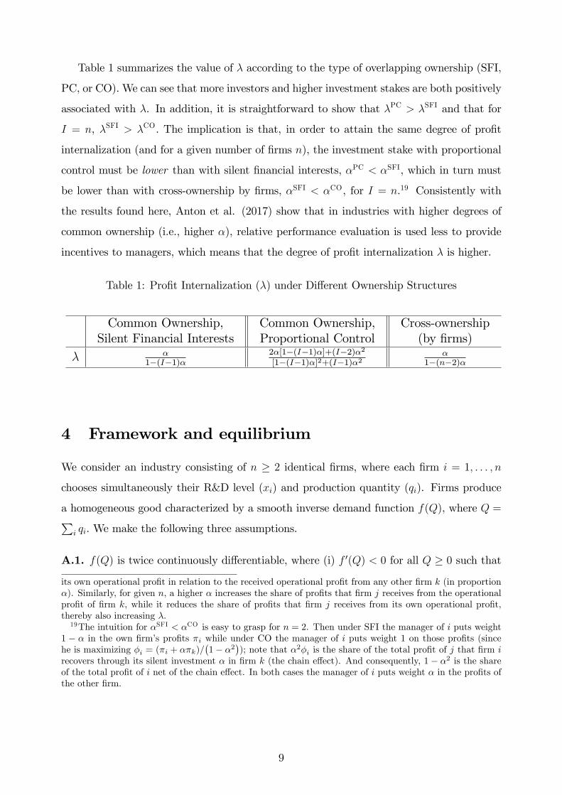
Table 1 summarizes the value of � according to the type of overlapping ownership (SFI,

PC, or CO). We can see that more investors and higher investment stakes are both positively

associated with �. In addition, it is straightforward to show that �PC > �SFI and that for

I = n, �SFI > �CO. The implication is that, in order to attain the same degree of pro�t

internalization (and for a given number of �rms n), the investment stake with proportional

control must be lower than with silent �nancial interests, �PC < �SFI, which in turn must

be lower than with cross-ownership by �rms, �SFI < �CO, for I = n.19 Consistently with

the results found here, Anton et al. (2017) show that in industries with higher degrees of

common ownership (i.e., higher �), relative performance evaluation is used less to provide

incentives to managers, which means that the degree of pro�t internalization � is higher.

Table 1: Pro�t Internalization (�) under Di¤erent Ownership Structures

Common Ownership,Silent Financial Interests

Common Ownership,Proportional Control

Cross-ownership(by �rms)

� �1�(I�1)�

2�[1�(I�1)�]+(I�2)�2[1�(I�1)�]2+(I�1)�2

�1�(n�2)�

4 Framework and equilibrium

We consider an industry consisting of n � 2 identical �rms, where each �rm i = 1; : : : ; n

chooses simultaneously their R&D level (xi) and production quantity (qi). Firms produce

a homogeneous good characterized by a smooth inverse demand function f(Q), where Q =Pi qi. We make the following three assumptions.

A.1. f(Q) is twice continuously di¤erentiable, where (i) f 0(Q) < 0 for all Q � 0 such that

its own operational pro�t in relation to the received operational pro�t from any other �rm k (in proportion�). Similarly, for given n, a higher � increases the share of pro�ts that �rm j receives from the operationalpro�t of �rm k, while it reduces the share of pro�ts that �rm j receives from its own operational pro�t,thereby also increasing �.19The intuition for �SFI < �CO is easy to grasp for n = 2. Then under SFI the manager of i puts weight

1 � � in the own �rm�s pro�ts �i while under CO the manager of i puts weight 1 on those pro�ts (sincehe is maximizing �i = (�i + ��k)/

�1� �2

�); note that �2�i is the share of the total pro�t of j that �rm i

recovers through its silent investment � in �rm k (the chain e¤ect). And consequently, 1� �2 is the shareof the total pro�t of i net of the chain e¤ect. In both cases the manager of i puts weight � in the pro�ts ofthe other �rm.

9

f(Q) > 0 and (ii) the elasticity of the slope of the inverse demand function,

�(Q) � Qf 00(Q)

f 0(Q);

is constant and equal to �.

The parameter � is the curvature (relative degree of concavity) of the inverse demand func-

tion, so demand is concave for � > 0 and is convex for � < 0. Furthermore, demand is

log-concave for 1 + � > 0 and is log-convex for 1 + � < 0. If 1 + � = 0, then demand is

both log-concave and log-convex.20 The family of inverse demand functions for which �(Q)

is constant, includes linear or constantly elastic cases, and can be represented as

f(Q) =

8><>:a� bQ�+1 if � 6= �1;

a� b logQ if � = �1;

here a is a nonnegative constant and b > 0 (resp., b < 0) if � � �1 (resp., � < �1).

A.2. The marginal production cost or innovation function of �rm i, or ci, is independent of

output and is decreasing in both own and rivals�R&D as follows: ci = c(xi+�P

j 6=i xj) > 0,

where c0 < 0, c00 � 0, and 0 � � � 1 for i 6= j.

A.3. The cost of R&D level xi is given by �(xi), where �(0) = 0, �0 > 0, and �00 � 0.

The parameter � represents the spillover level of the R&D activity. Since we focus on sym-

metric �rms, we assume symmetric spillover levels; moreover, R&D outcomes are imperfectly

appropriable to an extent that varies between 0 and 1. The intensity of spillover levels is

quite heterogeneous across industries. Bloom et al. (2013) �nd an average sensitivity of :4

to :5 of the stock of knowledge of a �rm in relation to the R&D investment of another �rm.

However, the dispersion of the estimates across industries is large.

Firm i�s pro�t is given by

�i = f(Q)qi � c

�xi + �

Xj 6=i

xj

�qi � �(xi);

20This class of demands features a constant pass-through from cost to price of (2 + �)�1 for a monopoly�rm (Bulow and P�eiderer 1983). We note that � is also related to the marginal consumer surplus fromincreasing output� that is, to MS = �f 0(Q)Q. Weyl and Fabinger (2013) argue that �MS � MS=(MS0Q))measures the curvature of the logarithm of demand. Under A.1, we can write 1=�MS = 1 + �.

10

and the objective function for the manager of �rm i is to maximize �i = �i + �P

k 6=i �k

choosing (qi; xi). The model represents distinct scenarios depending on the values of � and

�. When � 2 (0; 1) and � 2 [0; 1), �rms compete in the presence of partial ownership

interests and the R&D outcomes are imperfectly appropriable. When � 2 (0; 1) and � = 1,

�rms form a Research Joint Venture (RJV) under which all R&D outcomes are fully shared

among RJV members and the duplication of R&D e¤orts is avoided. When � = � = 1, �rms

form a �cartelized�RJV.21 If � = 0 then there is no overlapping ownership.

For markets with cross-shareholdings, a modi�ed HHI is proposed by Bresnahan and Sa-

lop (1986). This index corresponds to the market share�weighted Lerner index in a Cournot

market, and we write MHHI =�P

i siLi��. Here si and Li are (respectively) the market

share and Lerner index of �rm i; the term � denotes the demand (price) elasticity.22 In our

case it is easy to see that, for a given common marginal cost, (p� c)=p = MHHI=� at a

symmetric Cournot equilibrium; here MHHI = �=n for � = 1+�(n�1), which is monotone

in �. When � = 0 we have the standard HHI for a symmetric solution, 1=n, and if � = 1

then the modi�ed HHI is equal to 1.

Now we consider symmetric solutions of the game. Let B � 1+�(n� 1); then Bx is the

�e¤ective�investment that lowers costs for a �rm. Let � � 1 + ��(n� 1). Then �c0(Bx)q�

is the marginal e¤ect of investment by a �rm on its internalized pro�t �i. A symmetric

interior equilibrium (Q� = nq�; x�) must solve the �rst-order necessary conditions for the

maximization of �i (@�i=@qi = 0; @�i=@xi = 0):

f(Q�)� c(Bx�)

f(Q�)=MHHI�(Q�)

; (2)

�c0(Bx�)Q��

n= �0(x�): (3)

Here �(Q�) = �f(Q�)=(Q�f 0(Q�)) is the elasticity of demand. Equation (2) is the modi�ed

Cournot�Lerner pricing formula; expression (3) equates the marginal bene�t and marginal

cost of investment by a �rm taking into account its internalized pro�t �i. Note that both

MHHI and � are increasing in � and therefore respectively exert pressure to reduce output

21We follow here the terminology in Kamien et al. (1992). d�Aspremont and Jacquemin (1988) identifycooperation in R&D only, in our terminology, with � = 0 for output decisions and � = 1 for R&D decisionswith � 2 [0; 1]. This situation is termed an "R&D cartel" by Kamien et al. (1992). For the latter thesituation where � = 1 and � = 1 only for R&D decisions is termed "R&D cooperation".22Azar et al. (forthcoming) use the MHHI (in terms of control and share rights) to measure anticompetitive

incentives stemming from �nancial interests in the US airline industry. These authors �nd that, in year 2013,the increased market concentration generated by such �nancial interests was more than 10 times greaterthan the HHI increase above which mergers are likely to generate antitrust concerns.

11

(or increase prices and margins) and to increase investment.

Let second-order derivatives be denoted, at symmetric solutions, by @zizj�i � @2�i=@zi@zj

and @hzi�i � @2�i=@h@zi (with h = �, �, and z = q; x). We assume that the following

regularity conditions hold:

�q � @qiqi�i + (n� 1)@qiqj�i < 0;�x � @xixi�i + (n� 1)@xixj�i < 0;

and

� � �q�x � (@xiqi�i)2�B > 0: (4)

Together these conditions imply that (2) and (3) both have a unique solution if they hold

globally.23 Condition �q < 0 is a standard stability condition in a quantity Cournot game

(e.g., Dixit (1986)) and implies that @qiqi�i < 0. Condition�x = �c00(Bx�)q��B��00(x�) < 0

is the equivalent for the innovation choice (e.g., Leahy and Neary (1997), Vives (2008)). It

is noteworthy that �x < 0 requires that at least one of c00 and �00 be positive and implies

that @xixi�i < 0. (See Table 4 in the Appendix.)

If �(Q�; x�) > 0 then we say that the equilibrium is regular. In particular, we assume

that there is a unique regular symmetric interior equilibrium (Q�; x�).24 The focus of our

paper is on characterizing that equilibrium.

4.1 Model speci�cation examples

We will consider the well-known R&D model speci�cations� with linear (and therefore log-

concave) demand� of d�Aspremont�Jacquemin (AJ) and Kamien�Muller�Zang (KMZ); we

also consider a constant elasticity (CE) model with log-convex demand that is similar to the

Dasgupta and Stiglitz (1980) model but with spillover e¤ects. In AJ c(�) is linear and �(�) is

quadratic while in KMZ and CE, c(�) is strictly convex and �(�) linear. The AJ and the KMZ

model speci�cations are only equivalent for a subset of spillover values (which includes the

case of no spillovers and depends on the number of �rms).25 Table 2 summarizes these model

23This is so since they imply that the Jacobian of the FOC at the symmetric solution is negative de�nite.We have then that the Gale-Nikaido univalence conditions are ful�lled (see Section 2.5 in Vives 1999).24Provided �i is strictly concave in (qi; xi) and some mild boundary conditions hold, then an interior

equilibrium will exist. (Strict concavity of �i is ensured with the usual di¤erential second-order conditions,see A.1.2 in the online appendix.)25Furthermore, while in AJ the joint returns to scale (in R&D expenditure and number of �rms) are

decreasing, constant, or increasing when � is less than, equal to, or greater than 1=(n+1); in KMZ the jointreturns to scale are always nonincreasing if � � 1 (Proposition 4.1 in Amir 2000). See also Section A.2 ofthe online appendix.

12

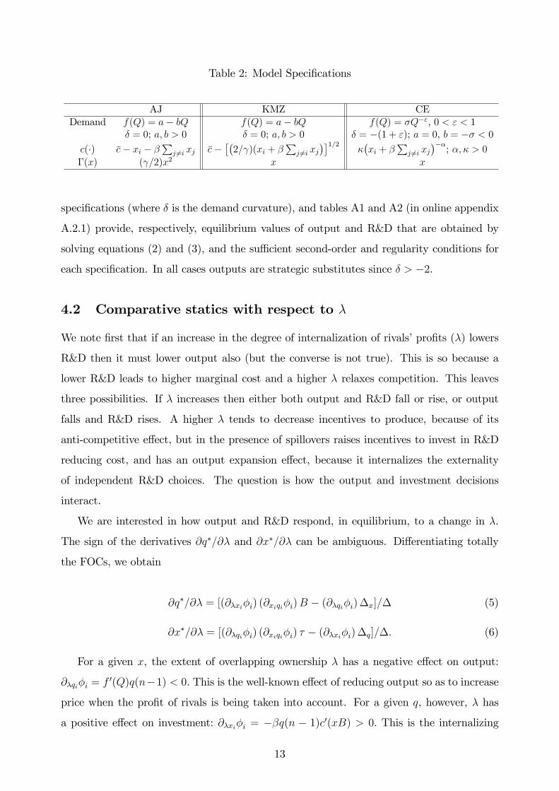
Table 2: Model Speci�cations

AJ KMZ CEDemand f(Q) = a� bQ f(Q) = a� bQ f(Q) = �Q�", 0 < " < 1

� = 0; a; b > 0 � = 0; a; b > 0 � = �(1 + "); a = 0, b = �� < 0c(�) �c� xi � �

Pj 6=i xj �c�

��2= )(xi + �

Pj 6=i xj

��1=2��xi + �

Pj 6=i xj

���; �; � > 0

�(x) ( =2)x2 x x

speci�cations (where � is the demand curvature), and tables A1 and A2 (in online appendix

A.2.1) provide, respectively, equilibrium values of output and R&D that are obtained by

solving equations (2) and (3), and the su¢ cient second-order and regularity conditions for

each speci�cation. In all cases outputs are strategic substitutes since � > �2.

4.2 Comparative statics with respect to �

We note �rst that if an increase in the degree of internalization of rivals�pro�ts (�) lowers

R&D then it must lower output also (but the converse is not true). This is so because a

lower R&D leads to higher marginal cost and a higher � relaxes competition. This leaves

three possibilities. If � increases then either both output and R&D fall or rise, or output

falls and R&D rises. A higher � tends to decrease incentives to produce, because of its

anti-competitive e¤ect, but in the presence of spillovers raises incentives to invest in R&D

reducing cost, and has an output expansion e¤ect, because it internalizes the externality

of independent R&D choices. The question is how the output and investment decisions

interact.

We are interested in how output and R&D respond, in equilibrium, to a change in �.

The sign of the derivatives @q�=@� and @x�=@� can be ambiguous. Di¤erentiating totally

the FOCs, we obtain

@q�=@� = [(@�xi�i) (@xiqi�i)B � (@�qi�i)�x]=� (5)

@x�=@� = [(@�qi�i) (@xiqi�i) � � (@�xi�i)�q]=�: (6)

For a given x, the extent of overlapping ownership � has a negative e¤ect on output:

@�qi�i = f 0(Q)q(n�1) < 0. This is the well-known e¤ect of reducing output so as to increase

price when the pro�t of rivals is being taken into account. For a given q, however, � has

a positive e¤ect on investment: @�xi�i = ��q(n � 1)c0(xB) > 0. This is the internalizing

13

e¤ect of spillovers with a higher �, and its strength depends directly on the size (�) of those

spillovers. The total impact of � on the equilibrium values of per-�rm output and R&D will

depend on which of the two previous e¤ects dominates. What is clear is that, if @x�=@� � 0,

then @q�=@� < 0 because @xiqi�i = �c0(xB) > 0 (output and R&D are complements for a

�rm). That is, an increase in R&D investment is necessary (but not su¢ cient) for output to

rise with increasing �. When � is small, the positive e¤ect on investment is small and so the

negative e¤ect on output dominates. Then q� decreases with � and, as a result, �rms invest

less also when � increases� given that the bene�t to �rms from investing in R&D decreases

proportionally with output.

We shall use RI to denote the region in which @q�=@� < 0 and @x�=@� � 0. If �

is su¢ ciently high, then the positive e¤ect on R&D reduces signi�cantly the unit cost of

production, which in turn stimulates output. Two e¤ects are present in this case. On the one

hand, �rms want to reduce output in order to increase competitors�pro�t and hence their

own �nancial pro�t. On the other hand, �rms now have incentives to produce more because

they are more e¢ cient. If the �rst e¤ect dominates, then @q�=@� < 0 and @x�=@� > 0 (we

label this region RII). But if the second e¤ect dominates, then @q�=@� > 0 and @x�=@� > 0

(region RIII). Which of these two cases arises in equilibrium will depend on the extent of

the spillovers. We �nd that, whereas RI always exists, regions RII and RIII might not exist.

We next derive the conditions and threshold values (in terms of �) that de�ne the bound-

aries of the regions characterizing the signs of @x�=@� (Lemma 1) and @q�=@� (Lemma 2).26

LEMMA 1 At equilibrium, sign f@x�=@�g = signf�(1 + n+ ��)� 1g:

COROLLARY 1 For any �xed � and for any � 2 [0; 1]; only RI exists (with @x�=@� � 0)

if and only if demand is convex enough� that is, i¤ � � �n=�.27 This statement holds for

any � in [0; 1] provided that � � �n.

We can interpret the critical spillover threshold for � in terms of the cost pass-through

coe¢ cient (i.e., the rate at which the price changes with marginal cost). This threshold is

equal to the industry-wide per-�rm cost pass-through coe¢ cient (P 0(c)=n) multiplied by the

internalized cost-reducing e¤ect of a unit increase in R&D expenditures by each �rm (�);

26The e¤ects on output and investment of changes in � do not depend on the assumption of a constant �.However, the characterization of the boundary in � space between RI and RII is made much simpler with �constant.27When � > �(n+ 1)=�, there exists a positive threshold of spillover above which @x�=@� > 0; however,

that threshold exceeds unity unless � > �n=�.

14

formally, we have sign�@x�=@�

= signf� � P 0(c)�=ng. Firms, in principle, should be less

interested in reducing costs when doing so translates, in e¤ect, into lower prices. Note that

P 0(c) is increasing with the degree of convexity of the demand.28

A consequence of Lemma 1 is that the threshold for spillovers to induce @x�=@� � 0

is decreasing (resp. increasing) in � when demand is concave (resp. convex)� that is, when

� > 0 (resp. � < 0).29

If demand is extremely convex, then increases in overlapping ownership are so restrictive

of output that they induce @x�=@� < 0, in which case only RI exists for any �. And since

MHHI = �=n, the applicable condition is that � � �(MHHI)�1. Corollary 1 implies that the

degree of demand convexity required for only RI to exist is decreasing in the concentration

measured by MHHI; in other words, the condition is less restrictive in markets that are more

concentrated. The corollary implies also that RII can exist only when quantities are strategic

substitutes.30 Indeed, if quantities are instead strategic complements (i.e., if @qiqj�i > 0,

which holds when � < �n(1+�)=�, then the condition � < �n=� always holds and only RIexists. When � is such that �n(1 + �)=� < � < �n=�, quantities are strategic substitutes

(as e.g. when demand is log-concave) but again only RI exists. If � > �n=�, then quantities

are strategic substitutes and RII exists (see Figure 5 in online appendix A.1.2 which depicts

the existence of regions RI and RII in (�; �) space together with conditions for outputs to

be strategic substitutes or complements).31

As regards the comparative statics on output, totally di¤erentiating the �rst-order con-

dition (FOC) with respect to � yields

sign f@q�=@�g = sign f@�qi�i +B(@xiqi�i)@x�=@�g ; (7)

here B = 1+�(n� 1) captures the e¤ect, on each �rm�s marginal cost, of a unit increase in

R&D by all �rms. At equilibrium, the impact on output of a higher degree of overlapping

28Let P (c) � f(nq�(c)); then P 0(c) = f 0(nq�)n�dq�=dc

�= n=[�(1 + �) + n]. Since the stability condition

�q < 0 holds when �(1 + �) + n > 0, it follows that P 0(c) > 0. Furthermore, the pass-through increaseswith the number of �rms when demand is log-concave (� > �1). See Weyl and Fabinger (2013).29So for � > 0, if @x�=@� > 0 for some � then that inequality must hold also for larger values of �.

Analogously: for � < 0, if @x�=@� < 0 for some � then that inequality holds also for larger values of �.30This is so when � > �(1 + �)n=� (see Table 4 in the Appendix), which holds for all � and n when

� > �2� in other words, the convexity of inverse demand must not be too high, which in turn implies thatmarginal revenue is strictly decreasing in output. It is worth noting that, in order for strict concavity of �iwith respect to qi (@qiqi�i < 0) at a symmetric equilibrium to be guaranteed for all �, we need the condition� > �2 (which guarantees strategic substitutability for all � and n). The concavity condition is � > �2n=�,and it is the strictest for � = 1 (in which case it reduces to � > �2).31It is worth noting that cost reduction e¤orts are strategic substitutes (@xixj�i < 0) provided that � > 0

(see Table 4 in the Appendix).

15

ownership depends directly on its e¤ect on marginal pro�t with respect to output (@�qi�i)

and indirectly through its e¤ect on the R&D e¤ort of each �rm at equilibrium. Recall that,

since @xiqi�i > 0, it follows that if @x�=@� � 0 then @q�=@� < 0 (RI). By Lemma 1 we

know that, if spillovers are su¢ ciently high and demand is not too convex, then @x�=@� > 0;

however, the sign of @q�=@� can be negative (RII) or positive (RIII).

We derive an inverse measure of R&D e¤ectiveness in terms of the model�s basic elastici-

ties. This measureH is an indirect function of �, since the equilibrium depends on �, and pro-

vides the appropriate threshold for the positive e¤ect of minority shareholdings on R&D in-

vestments to dominate its negative e¤ect on output. Let �(Bx�) � �c00(Bx�)Bx�=c0(Bx�) �

0 be the elasticity of the slope of the innovation function (i.e., the relative convexity of c(�))

evaluated at the e¤ective R&D, Bx�; and let y(x�) � �00(x�)x�=�0(x�) � 0 be the elasticity

of the slope of the investment cost function. Our regularity assumptions imply that either

c00 > 0 or �00 > 0 (or both). If �00(x�) > 0, let �(Q�; x�) � �(c0(Bx�))2=(f 0(Q�)�00(x�)) > 0

measure the relative e¤ectiveness of R&D.32 Note also that a higher ratio y=� means that

the investment is more e¤ective in reducing costs. Then H can be written as

H =1

�(Q�; x�)

�1 +

�(Bx�)

y(x�)

�;

evaluated at the equilibrium (Q�; x�). Note that H is positive and decreasing in the e¤ec-

tiveness of R&D as measured by � and by y=�.

LEMMA 2 Let B = 1 + �(n� 1). At equilibrium, sign f@q�=@�g = signf�B �Hg.

For � > 0 we have that the term H=� provides the appropriate threshold for B (the

e¤ect on each �rm�s marginal cost of a unit increase in R&D by all �rms) for a rise in � to

increase output. Therefore, if B > H=� then the positive e¤ect of overlapping ownership on

R&D investments dominates its negative e¤ect on output. The values of H for each model

speci�cation are presented in Table 3.33 Note that H is independent of � under the AJ and

KMZ models but is strictly increasing in � under the CE model. As we shall discuss later,

the relationship betweenH and � has important consequences for the optimal welfare policy.

It is worth noting that the e¤ectiveness of R&D increases with the elasticity of demand (b�1;

"�1) and with the elasticity of the innovation function ( �1; �) in the speci�ed models.

32As de�ned by Leahy and Neary (1997, Sec. V, p. 654).33In AJ, y = 1 and � = 0; in KMZ, y = 0 and � = 1=2; in CE, y = 0 and � = �+ 1.

16

Table 3: H (Inverse Measure of R&D E¤ectiveness)

AJ KMZ CEH b b B B

��+1�

�"

n�"��

We introduce the following mild assumption on H : [0; 1]! R+ (considered as a function

of �). H is continuous (see proof of Lemma 2).

A.4. H(�)=� is downward sloping.

Under assumption A.4, the equation B = H(�)=� has at most a unique positive solution

(since lim�!0H(�)=� =1). This assumption is su¢ cient but not necessary for uniqueness.

An (almost) necessary and su¢ cient condition for uniqueness is that H(�)=�B is decreasing

in � whenever B = H(�)=�. Denote that solution by �0; then, for � > �0 we have that

@q�=@� > 0. Assumption A.4 seems not to be restrictive in light of the model speci�cations

typically used in the literature; it is ful�lled in AJ and KMZ. In CE, H(�)=�B is strictly

decreasing in �. Assumption A.4 does not guarantee that there exists �0 < 1, so RIII may

fail to exist. We have that a solution �0 < 1 exists if n > H(1). Our next corollary states

the results formally.

COROLLARY 2 Under A.4, if n > H(1) then region RIII exists when � > �0 with �0 < 1

(where �0 is the unique positive solution to �B �H(�) = 0).

Using Lemmata 1 and 2� and observing that � > �n=� implies that 1+n+�� > 0� we

obtain the following result.

PROPOSITION 1 Let � = 1 + �(n � 1). Under assumptions A.1�A.3, if demand is

su¢ ciently convex (� � �n=�) then only region RI exists. Otherwise, assume A.1�A.4,

n > H(1), and let �(�) = 1=(1 + n+ ��) and �0 (�) be as de�ned in Corollary 2. Then the

following statements hold :

(i) if � � � (�) ; then @q�=@� < 0 and @x�=@� � 0 (RI);

(ii) if � (�) < � � �0 (�) ; then @q�=@� � 0 and @x�=@� > 0 (RII);

(iii) if � > �0 (�) ; then @q�=@� > 0 and @x�=@� > 0 (RIII).

17

Fig. 1. Spillover threshold values that limit regions RI, RII and RIII for agiven �.

Figure 1 depicts the three regions for the spillovers and the impact of changing �. Propo-

sition 1 implies that, for demand that is convex enough, the equilibrium is always in RI (and

that a higher � needs a less convex demand for the result to hold). Recall that when quan-

tities are strategic complements only RI exists. Otherwise, the equilibrium is in RI for a

low level of spillovers only. We write the thresholds as a function of �, � (�) and �0 (�), to

emphasize that Proposition 1 is for a given �: �(�) is decreasing or increasing in � according

to whether demand is concave (� > 0) or convex (� < 0); �0(�) is increasing in � if and only

if H is increasing in �. Recall that H is weakly increasing in � under all three model speci-

�cations: in AJ and KMZ, H is independent of �; in the CE model, H is strictly increasing

in �. In those cases the e¤ectiveness of R&D is weakly decreasing in the degree of pro�t

internalization �. Both � (�) and �0 (�) (for a given e¤ectiveness of R&D) are decreasing in

n.34 Furthermore, �0 is decreasing in the e¤ectiveness of R&D (H�1). More e¤ective R&D

increases RIII.

We can compare these results with those reported by Leahy and Neary (1997, Prop. 3),

in which there are no minority shareholdings and where R&D cooperation leads to more

R&D and output (as in our RIII) whenever spillovers are positive. Yet in our case, RIII

obtains only when spillovers are su¢ ciently high. Thus the �output cooperation� induced

by overlapping ownership requires su¢ ciently high spillovers in order to increase R&D and

output.

Finally, we are interested in analyzing the e¤ect of � on each �rm�s pro�t. We have that

signf��0(�)g = sign�� �c0(Bx�)

@x�

@�+ f 0(Q�)

@q�

@�

�: (8)

Given that @x�=@� > 0 and @q�=@� < 0 in RII, we can use (8) to show that� in this

region� ��0(�) > 0. The sign of the e¤ect of � on �� is less clear in RI (since in that region,

34For the AJ model, �0 is decreasing in n while in KMZ �rm entry has no e¤ect. In the CE model �0 maybe increasing in n for � close to 1.

18

@x�=@� < 0 and @q�=@� < 0) and in RIII (where @x�=@� > 0 and @q�=@� > 0). Nevertheless,

in online appendix A.1.2 we prove the following result.

PROPOSITION 2 At the symmetric equilibrium, the pro�t per �rm (��) increases with �.

According to this proposition, the positive e¤ect on price dominates the negative e¤ect

on R&D in RI, and conversely in RIII, so that pro�ts in both regions rise with the extent

of overlapping ownership. This means that investors and �rms have always incentives to

increase their interdependence. In the examples of ownership structures considered common

investors to the industry have incentives to increase their share of overlapping ownership

and similarly for �rms to increase the overlapping ownership stake in other �rms. This

is so provided the agreements are binding ones, because that feature allows the parties to

increase pro�ts.35 Before proceeding with the welfare analysis, we examine the e¤ect of �

on equilibrium values.

4.3 Comparative statics with respect to spillovers (�)

A su¢ cient (but not necessary) condition for increases in � to raise per-�rm R&D and output

is that @�xi�i > 0. It is not di¢ cult to see that signf@�xi�ig = signf�B=� ��(Bx�)g; here �

is the elasticity of the slope of the innovation function, which is nonnegative. For a positive

�, we have @�xi�i > 0 when the curvature (relative convexity) of the innovation function is

su¢ ciently low. The term �B=� = � (1 + � (n� 1)) = (1 + �� (n� 1)) increases with � for

� < 1, so it su¢ ces that � > � (since B=� = 1 for � = 0). Our next proposition follows.

PROPOSITION 3 If the curvature � of the innovation function is su¢ ciently low (� < �

would be low enough); then @q�=@� > 0 and @x�=@� > 0.

We can view the following results as corollaries. In AJ (where � = 0), stronger spillover

e¤ects raise the equilibrium values of output and R&D. In both KMZ (where � = 1=2) and

CE (where � = �+ 1 > 1) models it can be checked that, for � > 0, (i) q� increases with �

(with @q�=@� = 0 when � = 0), and (ii) x� increases (resp. decreases) with � for high (resp.

low) values of �.

35Farrell and Shapiro (1990), Flath (1991), and Reitman (1994) show that unilateral incentives to imple-ment SFI ownership structures may be lacking in Cournot competition with constant marginal costs. How-ever, Gilo et al. (2006) show that cross-ownership arrangements facilitate tacit collusion (in the symmetriccase) when the stakes are su¢ ciently high because they diminish incentives to deviate. For a di¤erenti-ated product market with two �rms, Karle et al. (2011) analyze the incentives of an investor to acquire acontrolling or noncontrolling stake in a competitor.

19

It is worth noting that � and � tend to be complements in raising x�. We have that

@2x�=@�@� > 0 in our three model speci�cations according to simulations.36 A higher level

of spillovers makes increasing � more e¤ective in raising x�.

5 Welfare analysis

Welfare in equilibrium is given by the sum of consumer surplus (CS) and industry pro�ts:

W (�) =

Z Q�

0

f(Q) dQ� c(Bx�)Q� � n�(x�):

We are interested in studying the e¤ect of the degree of overlapping ownership � on

welfare. Using the equilibrium conditions (2) and (3), we can write

W 0(�) = ���f 0(Q�)

@q�

@�+ (1� �)�(n� 1)c0(Bx�)@x

�

@�

�Q�: (9)

An increase in overlapping ownership alters equilibrium values of quantities and R&D

investments, and each additional unit of output and R&D has social value equal to (re-

spectively) �(�f 0(Q�))Q� and (1 � �)�(n � 1)(�c0(Bx�))Q�. Here Proposition 1 is useful.

In RI we have that W 0(�) < 0 because @x�=@� � 0 and @q�=@� < 0; in RIII, W 0(�) > 0

because @x�=@� > 0 and @q�=@� > 0. In RII, however, the e¤ect of � on welfare is positive

or negative according as whether the positive e¤ect of overlapping ownership on R&D does

or does not dominate its negative e¤ect on output level. Moreover, the e¤ect of � on CS is

positive (i.e., CS0(�) > 0) only when @q�=@� > 0 (i.e. in RIII). So even as consumers su¤er

from a higher degree of overlapping ownership in RI and RII, it bene�ts them in RIII. One

consequence is that optimal antitrust policy will tend to be stricter under the CS standard.

5.1 Socially optimal degree of overlapping ownership

Let �oCS and �oTS denote the optimal degree of pro�t internalization (overlapping ownership)

under the (respectively) CS and TS standard. In the three model speci�cations (AJ, KMZ,

CE), H is weakly increasing in � and W (�) is single peaked.37 In the CE model, numerical

simulations show that� for the parameter range in which the second-order condition (SOC)

36Furthermore, @2x�=@�@� can be shown positive when evaluated at � = � = 0.37W (�) is a function of one variable with only one stationary point that is a maximum (and hence a global

maximum). A mild additional condition is required in KMZ. See online appendix A.2.1.

20

and the regularity condition are satis�ed�W (�) is strictly concave.

We know from Proposition 1 that if demand is convex enough then only RI exists, in

which case no overlapping ownership is optimal regardless of spillover levels. However, the

condition for this to happen for any � (� � �n) is very restrictive globally since it never

holds for n � 2 if the regularity condition �q < 0 is required to hold for all � (which

needs � > �2). We �nd when � > �2 (and recall that this implies that quantities are

strategic substitutes for all � and n) that under some mild assumptions: if spillovers � are

low enough then overlapping ownership is also not optimal; and if spillovers are high enough

then the level of overlapping ownership can be positive in terms of both total surplus and

consumer surplus (i.e., �oTS > 0 and �oCS > 0). For intermediate values of � we have that

�oTS > �oCS = 0. It follows that more overlapping ownership should be allowed under the total

surplus standard (i.e., �oTS � �oCS). These results are stated formally in our next proposition.

PROPOSITION 4 Suppose that assumptions A.1�A.4 hold and let � > �2: Then if the

e¤ectiveness of R&D (H�1) is weakly decreasing in � and W (�) is single peaked, then there

are threshold values �� and �0(0) (with �� < �0(0)) such that

1. �oTS = �oCS = 0 if � � ��;

2. �oTS > �oCS = 0 if � 2 (��; �0(0)); and

3. �oTS � �oCS > 0 if � > �0(0).

In all cases, �oTS � �oCS. Furthermore, whenever both �oTS and �

oCS lie in (0; 1), then

�oTS; �oCS are strictly increasing in �.

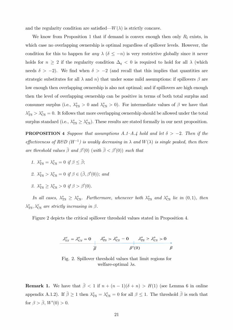
Figure 2 depicts the critical spillover threshold values stated in Proposition 4.

Fig. 2. Spillover threshold values that limit regions forwelfare-optimal �s.

Remark 1. We have that �� < 1 if n + (n � 1)(� + n) > H(1) (see Lemma 6 in online

appendix A.1.2). If �� � 1 then �oTS = �oCS = 0 for all � � 1. The threshold �� is such that

for � > ��, W 0(0) > 0.

21

Remark 2. The optimal �oTS is positively associated with the e¤ectiveness of R&D (H�1).

Furthermore, both �� and �0(0) are decreasing in n for a given e¤ectiveness of R&D. With

more �rms the scope, in terms of the range of spillovers, for welfare improving overlapping

ownership increases. Furthermore, the monotonicity of �oTS and �oCS with respect to � follows

since at the optimum both � and � are strategic complements in optimizing W and CS (i.e.

@2W=@�@� > 0 and @2CS=@�@� > 0).

Remark 3. Our single-peakedness assumption on W (�) ensures that �� is the minimum

threshold above which total surplus increases with � (i.e., for which � � �� implies �oTS = 0).

Remark 4. The assumption that H is weakly increasing in � ensures that � < �0(0)

implies �oCS = 0 and that �oTS � �oCS. In the particular case where � = �0(0) we have that

�oTS � �oCS � 0.

Relaxation of assumptions. If we relax the assumptions thatW (�) be single peaked and

that H be monotonic in �, then we can provide a weaker characterization of the regions

where overlapping ownership is socially optimal (Proposition 5) and we are able also to

characterize the extreme solution regions where �oCS = 0 or �oCS = �oTS = 1 (Proposition 6).

PROPOSITION 5 Let A.1�A.4 hold. If � > �(1 + n)=n; then there exist threshold values

� < �� < �0(0) (where � = inff1=(1 + n+��) : � 2 [0; 1]g) such that : (i) �oCS = �oTS = 0 for

� � �; (ii) �oTS > 0 for � > ��; and (iii) �oCS > 0 for � > �0(0).

Under the less restrictive assumptions we cannot ascertain what happens in the gap��; ��

�. From Proposition 1 it now follows that, when � � �, only RI exists because � >

�(1 + n)=n implies that 1 + n+ �� > 0 and � > �n. The threshold � depends on the sign

of �. If demand is concave (� > 0), then � = 1=[1 + n(1 + �)]; if demand is convex (� < 0),

then � = 1=(1 + n+ �). In both cases, � decreases with n (and tends to 0 with n).38 Parts

(ii) and (iii) follow as in Proposition 4: part (ii) because if � > �� then W 0(0) > 0 and so

�oTS > 0; and part (iii) because if � > �0(0) then @q�=@�j�=0 > 0 and �oCS > 0. (See online

appendix A.1.2 for details.)

PROPOSITION 6 Under A.1�A.4, the following statements hold :

(i) � < �0min implies �oCS = 0; and

(ii) � > �0max implies �oCS = �oTS = 1 provided that �

0max � 1.

38Note that in AJ and KMZ, demand is linear and � = 0; hence � = 1=(1+n). Under CE, � = � (1 + ") < 0and so � = 1=(n� ").

22

It follows that if �0 is independent of � (i.e. since H is) then �0min = �0max and we

have a bang-bang solution for �oCS, while when �0 is increasing in � (i.e. since H is) then

�0min = �0(0) as in Proposition 4.39

Proposition 6 determines when cartelization (� = 1) is optimal in terms of both consumer

and total surplus (in those cases, we are in RIII and welfare is increasing in �). In AJ and

KMZ, the term H is independent of �; thus the consumer surplus solution is bang-bang

under either model speci�cation. In both speci�cations it is clear that if �oCS > 0 then

necessarily �oTS = �oCS = 1. In the CE model, however, H and �0 are strictly increasing in �

and hence solutions of the form �oTS > �oCS > 0 are possible.40

The scope for a Research Joint Venture. An RJV can be understood as a situation

where spillovers are fully internalized (i.e., � = 1). If the RJV is �cartelized� then also

� = 1. This arrangement can be optimal only if RIII exists for � large (with �0max � 1) and

if @q�=@� > 0 and @x�=@� > 0 (which, by Proposition 3, holds if � < 1). Our next corollary

states the result.

COROLLARY 3 Again assume that A.1�A.4 hold. If �0max � 1 and if the innovation

function�s curvature is not too large (� < 1); then a cartelized RJV (� = � = 1) is optimal

in terms of consumer and total surplus.

The assumptions of the corollary are ful�lled in the AJ and KMZ models when RIII exists

( b < n and b < 1 are needed (respectively) to ensure that �0AJ and �0KMZ are less than

unity); and recall that � = 0 in AJ and � = 1=2 in KMZ. In CE, � = 1 is never socially

optimal because �0CE(1) < 1 only if " < �=(1 + 2�)� which would contradict the regularity

condition (see Table A2 in online appendix A.2.1).

Under some di¤erent conditions, an RJV with no overlapping ownership (� = 0 and � =

1) can be socially optimal in all three models (see Proposition A1 in online appendix A.2.1).

When W (�) is single peaked, no overlapping ownership is optimal if �� � 1.41 In contrast

with the AJ model, in both KMZ and CE we �nd that if � = 0 then greater R&D spillovers

reduce R&D expenditures (@x�=@� < 0) while having no e¤ect on output (@q�=@� = 0).

Although R&D expenditures are lower with higher �, the production costs of all �rms are

39This proposition is proved by noting that �0(�) is a continuous function on [0; 1] and so achieves amaximum (�0max) and a minimum (�0min) within that interval. If � < �

0min, then @q

�=@� < 0 for all � > 0and so �oCS = 0; if � > �0max, then @q

�=@� > 0 for all �. Since @q�=@� > 0 implies @x�=@� > 0 byequation (7), it follows that W 0(�) > 0 for all � by equation (9). Therefore, �oCS = �

oTS = 1 provided that

�0max � 1.40In the CE case, CS is globally concave in � when B > H(�)j�=0.41Satisfying that inequality requires b � n2 in AJ, b � n in KMZ, and an involved condition in CE.

23

also lower. In both cases, the greater R&D spillover�s negative e¤ect on R&D expenditures

is dominated by its positive e¤ect on the innovation function; as a result, � = 1 is also

socially optimal.

5.2 Comparative statics by model

We are interested in the comparative statics of the regions determining the scope for socially

e¢ cient overlapping ownership as described in Proposition 4. We are also interested in the

comparative statics on �oCS and �oTS in the speci�ed models. Table A3 reports the spillover

thresholds for AJ, KMZ and CE models.

Comparative statics on �0(0) and ��. The thresholds �0(0) and �� are decreasing in

� the number of �rms (n),

� the demand elasticity (b�1; "�1), and

� the innovation function�s elasticity ( �1; �).42

The results for �0(0) and for �� in relation to n (except in the CE model) are analytical,

the others according to numerical simulations.43 In KMZ, �0(0) is independent of n.

In terms of consumer surplus, in AJ it is optimal to suppress horizontal shareholdings

for any level of spillovers when �rm entry is insu¢ cient� that is, when n < b (since

then �0AJ > 1); in CE, suppression is optimal when n < "(2� + 1)=� (since �0CE > 1 for

n < "(2� + 1)�=�). We �nd also that �� may take values greater than 1 when there are

only a few �rms in the market.44 Therefore, for highly concentrated markets, no overlapping

ownership should be allowed for a wide range of spillovers. The reason is that the incentives

for �rms to �free ride�are stronger when the number of �rms increases because each �rm

can then appropriate the R&D e¤orts of a greater number of participants.45

Comparative statics on the socially optimal degree of overlapping ownership.

Our simulations generate three main �ndings. First, the socially optimal level of overlapping

ownership increases with the size of the spillovers, with the number of �rms (n), and with the

elasticities of demand (b�1; "�1) and of the innovation function ( �1; �). Note that larger

42Note that b�1 and �1 move together with the elasticities, respectively, of demand and the innovationfunctions.43Values for parameters are chosen so that the regularity condition and the SOCs are satis�ed.44In particular, from Table A3 (in online appendix A.2.1) it is straightforward to show that, in a duopoly,

�� > 1 when b > 4 in AJ, when b > 2 in KMZ, and when � > 2"=("2 � 7"+ 6) in CE.45In our model a high n means tougher competition and more incentives to free ride.

24

elasticities of demand and of the innovation function increase the e¤ectiveness of R&D,

which is positively associated with �oTS. Second, if the objective is to maximize consumer

surplus, then the comparative statics are qualitatively similar but the scope for minority

shareholdings is much lower. For example, increasing the number of �rms may not in itself

be su¢ cient for consumers to bene�t from overlapping ownership; in fact, this is the case

in KMZ. (Table A5 in online appendix A.2.1 provides more details of the simulations.)

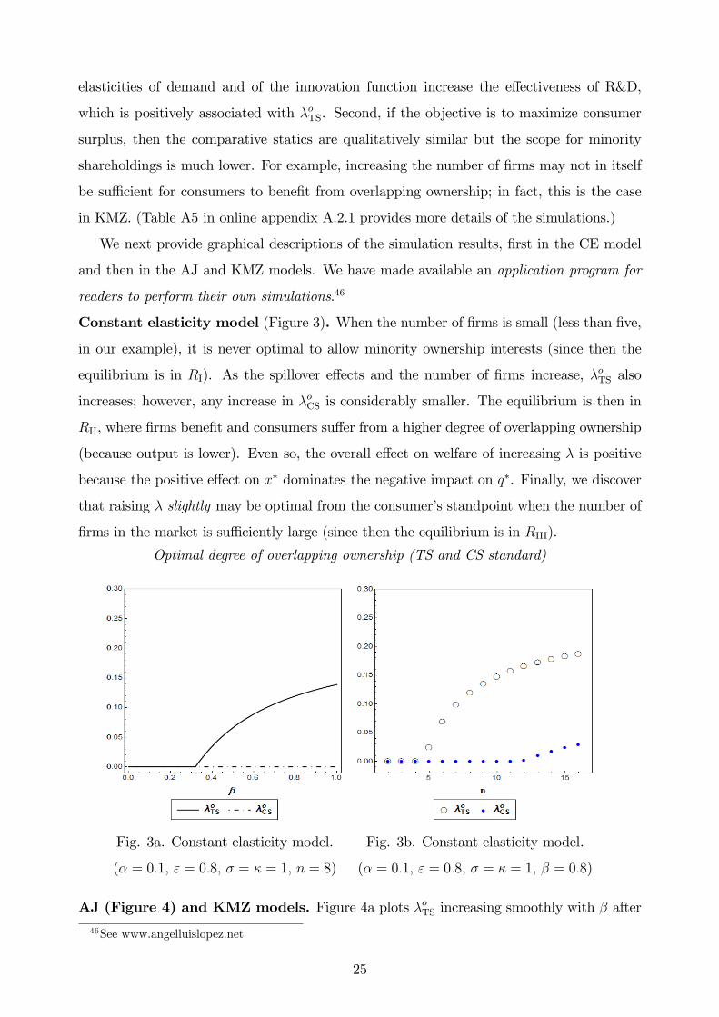
We next provide graphical descriptions of the simulation results, �rst in the CE model

and then in the AJ and KMZ models. We have made available an application program for

readers to perform their own simulations.46

Constant elasticity model (Figure 3). When the number of �rms is small (less than �ve,

in our example), it is never optimal to allow minority ownership interests (since then the

equilibrium is in RI). As the spillover e¤ects and the number of �rms increase, �oTS also

increases; however, any increase in �oCS is considerably smaller. The equilibrium is then in

RII, where �rms bene�t and consumers su¤er from a higher degree of overlapping ownership

(because output is lower). Even so, the overall e¤ect on welfare of increasing � is positive

because the positive e¤ect on x� dominates the negative impact on q�. Finally, we discover

that raising � slightly may be optimal from the consumer�s standpoint when the number of

�rms in the market is su¢ ciently large (since then the equilibrium is in RIII).

Optimal degree of overlapping ownership (TS and CS standard)

Fig. 3a. Constant elasticity model.

(� = 0:1, " = 0:8, � = � = 1, n = 8)

Fig. 3b. Constant elasticity model.

(� = 0:1, " = 0:8, � = � = 1, � = 0:8)

AJ (Figure 4) and KMZ models. Figure 4a plots �oTS increasing smoothly with � after46See www.angelluislopez.net

25

� = 0:4 and up to �0 = 0:91 where �oCS jumps to 1. In online appendix A.2.1 we can see

a snapshot of our app that illustrates the simulation for � = 0:5 and n = 6. In this case

the welfare translation of the increase in � shows in a decreasing consumer surplus and

increasing per-�rm pro�t that results in an interior solution for welfare �oTS > 0. Figure 4b

shows that �oTS increases with n, and �oCS does jump to 1 only if n is su¢ ciently large (our

example, where � = 0:8, requires n > 6).

Optimal degree of overlapping ownership (TS and CS standard)

Fig. 4a. AJ model.

( = 8:5, n = 6, b = 0:6.)

Fig. 4b. AJ model.

( = 7, � = 0:8, b = 0:6.)

Figures for the KMZ model are presented in online appendix A.2.1. In KMZ, increasing

n a¤ects neither �0 nor (as a result) signfCS0(�)g. Therefore, in contrast to AJ, where for a

su¢ ciently large number of �rms we may have �oCS = 1, in KMZ for a given � < �0KMZ, we

have �oCS = 0 irrespective of the number of �rms. Furthermore, in KMZ although �oTS also

increases with n , its rate of change decreases with n (see Fig. A6b where �oTS converges to

a value below one when n increases).

6 Two-stage model

We extend the �simultaneous action�(static) model of R&D investment to a strategic com-

mitment (two-stage) model and �nd that our results are (with some caveats) robust to this

extension. In the �rst stage, every �rm i commits to investing an amount xi into R&D. In

the second stage� and for given observable level of R&D expenditures� �rms compete in

the product market. We solve for the model�s subgame-perfect equilibrium as a function

26

of �.

6.1 Equilibrium and strategic e¤ects

Let x = [x1; x2; : : : ; xn] be the �rst-stage R&D pro�le and let q = [q1; q2; : : : ; qn] be the

second-stage output pro�le. Let q�i (x) denote �rm i�s (interior) output equilibrium value of

the second-stage game associated with the R&D pro�le x. Then, for all i, we have

@

@qi�i(q

�(x);x) = 0: (10)

In the �rst stage, the �rst-order necessary conditions for an interior equilibrium are (for

i 6= j and i; j = 1; 2; : : : ; n)

@

@xi�i(q

�(x);x) +Xj 6=i

@

@qj�i(q

�(x);x)@

@xiq�j (x) = 0: (11)

The equilibrium R&D pro�le x� is characterized by the system of equations (10) and (11)�

provided the second-order conditions hold. Let q� = q�(x�); then fx�;q�g is the subgame-

perfect equilibrium path of the two-stage game. The second term in equation (11) is the

strategic e¤ect on pro�ts of investment. Evaluating at a symmetric equilibrium, where

q�i = q� and x�i = x� for all i, it is easy to see that @�i=@qj < 0, j 6= i, but the sign of

@q�j=@xi is ambiguous:

sign

�@q�j@xi

�= signf� � ~�(�)g; where ~�(�) �

@qiqj�i@qiqi�i

=n(1 + �) + ��

2n+ ��:

Note that the threshold ~� 2 (0; 1] depends only on �, n, and �. The inequality ~�(�) >

0 holds only if production decisions are strategic substitutes (i.e., only if @qiqj�i < 0).

Furthermore, ~�(�) < 1 for � < 1 and ~�(�)! 1 as �! 1.

We can also conduct comparative statics on the threshold value ~�(�). Under assump-

tion A.1 and from the expression for ~�, it is straightforward to show the following result

which highlights the crucial role played by demand curvature �.

LEMMA 3 For � < 1; the threshold ~�: decreases (resp. increases) with n if demand is

concave (resp. convex); increases with � if � > �2; and increases with �.

When the stability condition in output is satis�ed (�q < 0), we have @q�i =@xi > 0. So if

a �rm increases its investment in R&D in the �rst stage, then it will increase its output in

27

the second stage. At the same time we have that @q�j=@xi > 0 when quantities are strategic

complements (since then ~� < 0). In the case of strategic substitutes, @q�j=@xi > 0 only if

� > ~�(�). When a �rm increases the amount invested in R&D, it exerts two opposite e¤ects

on the output decision of rival �rms. There is a positive e¤ect because rival �rms become

more e¢ cient owing to the presence of spillovers. Yet there is also a negative e¤ect because

the reaction of rivals to �rm i�s higher quantity is to reduce their own output via competing

in the market for strategic substitutes. If spillover e¤ects are strong enough that � > ~�(�),

then the positive e¤ect outweighs the negative e¤ect; this outcome implies that @q�j=@xi > 0.

We can show (using A.1) that the strategic e¤ect of investment, at a symmetric equilib-

rium, is as follows:47

� (n� 1) @�i@qj

@q�j@xi

= � (n� 1) c0(Bx�)q�!(�)(~�(�)� �), where (12)

!(�) =�

n

�2n+ ��

n+ �(1 + �)

�> 0: (13)

Hence we may write the FOC (11) for � 2 [0; 1) as

�c0(Bx�)�� + (n� 1)!(�)(~�(�)� �)

�q� � �0(x�) = 0: (14)

Since @�i=@qj < 0, it follows that

signf g = �sign�@q�j=@xi

= signf~�(�)� �g:

Thus the strategic e¤ect is positive if production decisions are strategic substitutes and if

� < ~�. In this case, there are incentives to overinvest because increasing investment reduces

the rival�s output. Then, as shown by Leahy and Neary (1997, Prop. 1) for � = 0, equations

(10) and (14) together imply that output and R&D are higher in the two-stage model than in

the static model.48 Since each �rm expects a higher �rst-stage investment in R&D to reduce

the second-stage output of rival �rms, each �rm is then led to increase their �rst-stage R&D

investments, which in turn boosts output in the second stage (@q�i =@xi > 0). Observe that

~�(1) = 1: if there is no RJV (� < 1) then, for high levels of �, the strategic e¤ect is always

47The stability condition, �q < 0, requires that n+�(1+�) > 0 and implies that 2n+�� > 0. Therefore,!(�) > 0.48This result is derived under assumptions yielding a unique symmetric equilibrium and such that the

two models�respective pro�t functions satisfy the Seade stability condition with respect to R&D� namely,that the marginal pro�t of each �rm with respect to R&D must decrease with a uniform increase in R&Dby all �rms.

28

positive (� < ~�). In contrast, if � exceeds ~� then the strategic e¤ect is negative; hence both

output and R&D are lower in the two-stage model than in the static model.

Remark 5. Recall that � > �2 if we want the regularity condition �q < 0 for all �. We

have then that the strategic e¤ect will tend to be positive in industries with a higher degree

of overlapping ownership since then @~�=@� > 0 according to Lemma 3.

The sign of the strategic e¤ect determines whether investment in cost reduction leads to

a "top dog" or a "puppy dog" strategy in the terminology of Fudenberg and Tirole (1984).

In the �rst case there is overinvestment and in the second underinvestment in relation to

the simultaneous move case.

6.2 Comparative statics with respect to �

Next we analyze how the degree of overlapping ownership a¤ects the decisions on output and

R&D that are made in equilibrium. By using (12) and by totally di¤erentiating the system

formed by (10) and (11) before evaluating it at a symmetric equilibrium, we can solve both

for @q�=@� and for @x�=@� under regularity conditions. Let s(�) � !(�)�~�(�)� �

�. We

obtain the following result.

LEMMA 4 In the two-stage model :

sign f@x�=@�g = sign�(� + s0(�))P 0(c)�1n� [� + (n� 1)s(�)]

; (15)

sign f@q�=@�g = sign�(� + s0(�))B � �H(�)

: (16)

Moreover, if @x�=@� � 0 then @q�=@� < 0.

So once again we �nd that allowing for some additional degree of overlapping ownership

will increase output only if it also boosts R&D. From (15) we obtain that @x�=@� > 0 if

and only if � > �2S (see the proof of this lemma in online appendix A.1.3 for an expression

for �2S).49 We assume that there is at most a unique positive �, denoted �2S0, that solves

the equation (� + s0(�))B = �H(�).50

49When there is no strategic e¤ect (i.e. !(�) = 0), then �2S equals the corresponding expression inProposition 1.50In AJ there exists a unique �2S

0< 1 when n is su¢ ciently large� or when and b are su¢ ciently

low� and � is su¢ ciently large. In KMZ for high � and su¢ ciently low and b, there exists a unique �2S0

that is nearly (but still less than) 1. In CE there seems to be no solution, in which case region RIII doesnot exist.

29

We are now in a position to derive the threshold values of spillovers that determine

the sign of the e¤ect, at equilibrium, of � on R&D and output. We have @q�=@� � 0

for � 2 [0; �2S0] and @q�=@� > 0 for � 2 (�2S0; 1]. Therefore: RI (where @x�=@� � 0 and

@q�=@� < 0) occurs when � � �2S; RII (where @q�=@� � 0 and @x�=@� > 0) occurs for

� 2 (�2S; �2S0]; and RIII (where @q�=@� > 0 and @x�=@� > 0) occurs when � > �2S0 with

�2S0 < 1:These results extend Proposition 1 to the two-stage model and we can derive the

threshold values for each of the model speci�cations considered in the paper (see online

appendix A.2.2).

Our �ndings can be compared to those of Leahy and Neary (1997, Prop. 3). Those authors

show that if cooperation happens only at the R&D then the result is reduced output and

R&D� unless spillovers are high enough, in which case �rms increase both output and R&D.

These two results correspond to regions RI and RIII, respectively. In addition, we identify

region RII: where cooperation driven by overlapping ownership leads to less output and more

R&D. Another di¤erence is that, in Leahy and Neary�s model, the spillover threshold above

which cooperation leads to more output and R&D lies strictly between 0 and 1. In contrast,

here (as in the simultaneous choice case) there is no guarantee that RIII exists; that is, �2S0

may lie above 1.

6.3 Welfare

We show that our welfare analysis is generally robust to the two-stage model. The only

caveat is that the presence of a strategic e¤ect of investment induces the �rms to underinvest

-puppy dog ploy- when spillovers are high (negative strategic e¤ect). In this case the socially

optimal level of overlapping ownership is higher than in the static model. This is consistent

with our �nding that the strategic e¤ect will tend to be positive in industries with a higher

degree of overlapping ownership.

Now we have (see the proof of Lemma 7 in online appendix A.1.3) that

W 0(�) = ���f 0(Q�)

@q�

@�+�(1� �)� � !(�)(~�(�)� �)

�(n� 1)c0(Bx�)@x

�

@�

�Q�:

Hence the term !(�)(~�(�) � �) coming from the strategic e¤ect of investment plays an

important role in determining the impact of overlapping ownership on welfare. When the

strategic e¤ect is negative (� > ~�(�)), the two-stage model behaves like the simultaneous

model (W 0(�) < 0 in RI,W 0(�) > 0 in RIII, andW 0(�) either positive or negative (depending

30

on �) in RII) but there are social incentives to increase more �. In this case the impact of �

on welfare through a change in R&D is magni�ed. Yet when the strategic e¤ect is positive

and spillovers are su¢ ciently low (though not necessarily close to zero),W 0(�) < 0 in RII and

W 0(�) can be positive or negative in RI and in RIII. In this case the impact of � on welfare

through a change in R&D is dampened. A consequence of some interest is that, in RIII�

where @x�=@� > 0 and @q�=@� > 0, so consumer surplus increases with � (indeed, � = 1 is

optimal for consumers)� total surplus can be decreasing in � for su¢ ciently high �.51 Then,

in stark contrast to the simultaneous model and owing to the strategic e¤ect of investment,

for some spillover values it may be that �oCS = 1 > �oTS > 0. The resulting overinvestment

increases output (and is good for consumer surplus) but comes at the cost of reducing �rms�

pro�ts, reducing total surplus, and �overshooting�marginal cost reductions. We illustrate

this possibility under the AJ and KMZ model speci�cations in Figure A12 for AJ and Figure

A13 for KMZ in the online appendix A.2.2.52 Similarly as in the simultaneous case, there

is a threshold value ��2S for which �oTS > 0 if � > ��2S; the condition under which ��2S < 1 is

given by Lemma 7 in online appendix A.1.3.53

In summary, the welfare results of the simultaneous model are robust to the two-stage

speci�cation with the proviso that for high spillovers a higher degree of overlapping owner-

ship should be allowed. In this case the strategic e¤ect is negative and there are incentives

to underinvest; then it pays to increase � in order to stimulate investment and output.54

This need not be the case for low values of spillovers, in which case the incentive is typically

to overinvest.

Simulations The online appendix A.2.2 presents our simulations of the three considered

models. These simulations con�rm the qualitative results obtained in the static model, but

with the two above mentioned caveats: (i) in the two-stage model, the socially optimal level

of overlapping ownership tends to be higher when spillovers are high; and (ii) in some cases

the consumer surplus standard may call for more cooperation than does the total surplus

standard (i.e., �oCS > �oTS > 0). We �nd also that as in the simultaneous case, for the three

models considered, the spillover threshold over which some overlapping ownership is optimal

��2S decreases with the number of �rms, the elasticity of demand and with the elasticity of

51For � < 1, we have (1� �)� � !(�)(~�(�)� �)j�=1 = �(1� �) < 0.52In CE, as in the simultaneous model, ��CS is usually zero or very close to zero.53If the condition holds then W 0(0)j�=1 > 0, in which case there exists a su¢ ciently large spillover value

for which some degree of overlapping ownership is welfare enhancing.54Note that ~�(�)! 1 as �! 1 and so ~�(�) > � for � high enough and the strategic e¤ect turns positive.

31

the innovation function.

Summary When spillovers are above a given threshold, �rms invest less in R&D and

produce less in the two-stage than in the static model; hence the strategic e¤ect of investment

becomes negative. In this case, the social gains from a higher degree of overlapping ownership

that induces �rms to invest are even greater. We also characterize how these gains are a¤ected

by the number of �rms, the extent of overlapping ownership, and the curvature of the inverse

demand function. For a low level of spillovers, the strategic e¤ect is positive and there are

incentives to overinvest. Then it need no longer be true that the consumer surplus standard

calls for reduced overlapping ownership in relation to the total surplus standpoint.

7 Bertrand competition

In this section we test the robustness of our results to Bertrand pricing with di¤erentiated

products. To advance the conclusion, the results obtained in the Cournot model are robust.

Two interesting features of the Bertrand model are the following. First, the socially optimal

level of overlapping ownership tends to have a U-shaped relationship with the degree of

product di¤erentiation (market spillovers). This is so since the closeness of the products

has typically an ambiguous e¤ect on the impact of � on R&D and output, but with positive

impact for low or high market spillovers. Second, the strategic e¤ect typically plays towards

underinvestment even for moderate levels of spillovers (this is consistent with the analysis

in Leahy and Neary 1997). For a fuller and detailed development of the analysis and proofs

see online appendix B.

Consider an industry with n di¤erentiated products, each produced by one �rm. The

demand for good i is given by qi = Di(p) where p is the vector of prices.

Assumption 1B. For any product i, the function Di (�) is smooth whenever positive,

downward sloping, products are (strict) gross substitutes @Di=@pj > 0, j 6= i, and the demand

system D (�) is symmetric with negative de�nite Jacobian.

Under assumption 1B the demand system can be obtained from a representative con-

sumer with quasilinear utility and can be inverted to obtain inverse demands.55 Furthermore,

it follows that the demand for a variety when all �rms set the same price (the Chamber-

linian DD function) is downward sloping since the own-price e¤ect dominates the cross-price

55See Vives (1999) Section 6.3 and pp. 144-148.

32

e¤ects: v � @Di=@pi + (n � 1)@Dj=@pi < 0, j 6= i. A fortiori, and for further reference, it

follows that v� � @Di=@pi + �(n � 1)@Dj=@pi < 0. The innovation function is as before;

�rm i�s pro�t is given by

�i =

pi � c

xi + �

Pj 6=i

xj

!!Di(p)� �(xi).

and the objective function for the manager of �rm i is �i = �i + �P

k 6=i �k. The �rst-order

conditions for an interior symmetric equilibrium (p�; x�) yield

p� � c(Bx�)

p�=

1

�i � �(n� 1)�ik; (17)

�c0(Bx�)q�� = �0(x�): (18)

Here �i = �@Di(p

�)@pi

p�

Di(p�)and �ik =

@Dk(p�)

@pi

p�

Dk(p�); k 6= i.

We assume parallel regularity conditions to the Cournot case which imply as before that

(17) and (18) both have a unique symmetric solution if the conditions hold globally, and

we assume that a symmetric regular equilibrium exists. We consider two leading examples

corresponding, respectively, to the analog of the AJ and CE models with (symmetric) prod-

uct di¤erentiation. The demand systems of the examples can be derived from a symmetric

(sub)utility function of a representative consumer on the vector q of the quantities of the

varieties of the di¤erentiated product. The �rst example follows our base speci�cation with

quasilinear utility while the second presents a robustness analysis in a CES model à la Dixit

and Stiglitz (1977).

Linear example (with quasilinear utility) The demand for product i is given by

Di(p) = a � bpi +mP

j 6=i pj with a > 0; b > m > 0, assumption 1B holds, and as before

ci = �c� xi � �P

j 6=i xj and �(x) = ( =2)x2.56

56This demand system can be obtained from

U(q) = u1nPi=1

qi �1

2

u2

nPi=1

q2i + 2u3Pj 6=iqiqj

!,

where u2 > u3 > 0 and a; b and m are a function of u1, u2, u3 (Vives 1999, pp. 146-147.) In order to ensurepositive outputs we assume that u1 � �c > 0. The products range from independent (u3 = 0) to perfectsubstitutes (u3 = u2).

33

Constant elasticity example (with non-quasilinear utility) The demand for

product i is given by

Di(p) =p�1��=(1��)iPnj=1 p

��=(1��)j

S,

where � 2 (0; 1), and S is the total spending on the di¤erentiated product varieties. Note

that � � 1=(1� �) is the constant elasticity of substitution between any two products. As

� ! 1, products become perfect substitutes (� ! 1), while as � ! 0, products become

independent (� ! 1). We have that �i = 1+(1�n�1)= (��1 � 1) and �ik = n�1�= (1� �).57

As before, ci = �(xi + �P

j 6=i xj)�� with �,� > 0 and �(xi) = xi.58

7.1 Comparative statics with respect to �

In the Bertrand model we have that: for a given investment level, � has a positive e¤ect on

price because products are gross substitutes, @�pi�i = (n� 1)(p� c)@Dk=@pi > 0, k 6= i; for

a given price, � has a positive e¤ect on investment as before, @�xi�i = ��q(n�1)c0 � 0; and

again the total impact of � on the equilibrium values of price and R&D will depend on which

of the two previous e¤ects dominates. We have also that if @x�=@� � 0, then @p�=@� > 0,

because @xipi�i = � (@Di=@pi + ��(n� 1)@Dk=@pi) c0 < 0, k 6= i, since v < 0 and �� < 1

(price and R&D are substitutes for a �rm). The upshot is that a similar result to Lemmata

1 and 2 can be established here (see Lemma B2 in online appendix B). We �nd that:

(i) sign f@x�=@�g = sign�� � P 0(c) jvj �v�2� @Dk=@pi

where P 0(c) � dp�=dc > 0 is the

cost pass-through coe¢ cient;

(ii) sign f@p�=@�g = sign fH � �Bg, where H = (1 + �=y) =�, and for �00 > 0; � �

(v�c0)2 = (�00@Dk=@pi) > 0. The di¤erence with respect to the Cournot model is that here

the expression for the relative e¤ectiveness of R&D (�) takes into account the fact that

products are di¤erentiated (and the term (f 0)�1 is replaced by v2� (@Dk=@pi)�1).

We can de�ne the three regions as in the Cournot case: RI, where @x�=@� � 0 and

@p�=@� > 0; RII where @x�=@� > 0 and @p�=@� > 0; RIII where @x�=@� > 0 and @p�=@� <

57The demand system is obtained from maximizing

V (q; q0) =

�nPi=1

q�i

�1=�q�0 ,

with � 2 (0; 1), � > 0, and q0 the numéraire good, subject to the budget constraint q0 +Pn

i=1 piqi = Y ,where Y is aggregate income. Then S = Y= (1 + �) :58In this model it is worth noting that the regularity condition require that � < 1. That is, the cartel

problem is ill-de�ned with �rms having incentives to set in�nite prices. See online appendix B.

34

0. Regarding RI, because of gross substitutes (@Dk(p�)=@pi > 0, k 6= i), we can have

@x�=@� < 0 for all �. Regarding the critical spillover threshold that bounds RII and RIII,

note that here, as in Cournot, assumption A.4 implies that the equation H � �B = 0 has a

unique positive solution, which again we may denote by �0 (�). It follows that for � > �0 (�),

@p�=@� < 0. Furthermore, RIII exists (because �0 < 1) when n > H(1). As before, �0 is

decreasing in the e¤ectiveness of R&D, H�1.

In online appendix B we state the equivalent of Proposition 1 characterizing explicitly

the regions for the linear and constant elasticity cases (see, respectively, propositions BL1

and BCE1).59 We �nd that the thresholds that bound the regions RI, RII and RIII, � (�) and

�0 (�) respectively, are increasing in � in both cases (see �gures B1 and B11 in the online

appendix), but while both � (�) and �0 (�) are hump-shaped in u3=u2 in the linear case,

both are decreasing in � in the constant elasticity model. In the linear model we have that

� (�) = �0 (�) = 0 both when products are independent (u3=u2 = 0) or perfect substitutes

(u3=u2 = 1), in which case only RIII exists. This is so since when goods are independent to

increase � always increases x� and q� since market power is already at its maximum level

while when products tend to be homogeneous competition is so intense that the impact

of increasing � in market power is small.60 In the constant elasticity model we also have

similarly that � (�) = �0 (�) = 0 for � = 1 but not when � = 0. This is so because the local

monopoly solution is ill-de�ned as �rms would like to charge an in�nite price as �! 0 (the

elasticity of demand �i becomes unity).61 The comparative static results for �0 follow since

H (inverse e¤ectiveness of R&D) has the same properties. The e¤ectiveness of R&D H�1 is

U-shaped in the closeness of the products as in the linear case (with H�1 !1 both when

products are close to independent and close to perfect substitutes). In the constant elasticity

case H�1 is always increasing in the elasticity of substitution of the varieties � = 1= (1� �).

In sum, the closeness of the products (or the degree of market spillovers) has typically an

ambiguous e¤ect on the impact of � on x� and q�, with positive impact for low or high

market spillovers.

We �nd that @2x�=@�@� > 0 in the constant elasticity model and, according to simula-

tions, also for the linear model.

59As in the Cournot model, in the linear Bertrand model, assumption A.4 is ful�lled and in the constantelasticity version we have that H (�) =�B is decreasing in �.60When u3 ! u2, we are always in RIII since then sign f@x�=@�g = sign f@p�=@�g = sign f�c� u1g < 0.61In both the linear and constant elasticity cases the products do not have to be too close in order for the

regularity conditions to hold.

35

7.2 Welfare analysis

Welfare (with quasilinear utility) at a symmetric equilibrium is given by W = U(q�) �

c(Bx�)nq� � n�(x�), where q� is the equilibrium output vector and U is the utility of

a representative consumer, assumed to be smooth and strictly concave (with a negative

de�nite Hessian). By di¤erentiating with respect to � and from the maximization problem

of the consumer we have that pi = @U=@qi, and at an equilibrium

W 0(�) =

�(p� � c(Bx�))

@q�

@�� (c0(Bx�)Bq� + �0(x�)) @x

�

@�

�n,

which may be written as

W 0(�) = ��v

v�

@p�

@�+ (1� �)�(n� 1)c0(Bx�)@x

�

@�

�nq�. (19)

Thus, since v=v� > 0, we have as in the Cournot case that in RI , where @x�=@� < 0 and

@p�=@� > 0 (so @q�=@� < 0), W 0(�) < 0; in RII, where @x�=@� > 0 and @p�=@� > 0 (so

@q�=@� < 0), W 0(�) 7 0; and in RIII, where @x�=@� > 0 and @p�=@� < 0 (so @q�=@� > 0),W 0(�) > 0.

It is worth noting that when products are independent, with the local monopoly problem

well de�ned, and � > 0 we have always that �oTS = �oCS = 1. This is so since with local

monopolies, as stated above, increasing � does not a¤ect the degree of monopoly and helps

internalizing the investment externality (if � = 0, then � has no impact on total surplus or

consumer surplus).

We can check that propositions 2 and 4 hold for the Bertrand linear and constant elastic-

ity models, and that thresholds �� (above which �oTS > 0) and �0 (0) (above which �oCS > 0)

are strictly decreasing in n.62 Furthermore, �� in the linear case is hump-shaped in u3=u2

since �� = 0 both for u3=u2 = 0 and u3=u2 = 1, while in the constant elasticity case is

monotone decreasing in � (or � = 1= (1� �)) according to simulations.

The socially optimal � increases with � and with n, and in terms of consumer surplus

in the linear model, the scope for overlapping ownership is lower. Furthermore, both �oTS

and �oCS have a U-shaped relationship with respect the degree of product di¤erentiation

in the linear case. Indeed, both �oTS and �oCS tend to 1 as products become independent

62In the constant elasticity case with non-quasilinear utility, from the resource constraint q0 = Y �ncq�nx,utility at a symmetric equilibrium is V (q�; Y � nc(Bx�)q� � nx�) = n1=�q� [S(1 + �)� nc(Bx�)q� � nx�]�.We can derive V 0 (�) accordingly (see online appendix B.4.2). We use the notation �oTS also for this casedespite the fact that we have V instead of TS.

36

(u3=u2 ! 0 ) and they both increase also as they tend to perfectly homogeneous (u3 ! u2).

In the constant elasticity model we have that �oTS grows always with � (when positive)

because the local monopoly solution (the case � = 0) is ill-de�ned as explained. Figures

B5-6 and B15 in online appendix B illustrate the examples.

We have, therefore, that the e¤ect of the intensity of competition, as measured by the

degree of product di¤erentiation, on the optimal degree of pro�t internalization will typically

be non-monotone. Note that with product di¤erentiation we can increase the intensity of

competition keeping the number of �rms constant by increasing the substitutability of the

products. This allows to isolate the e¤ect of the degree of rivalry.

7.3 Two-stage competition

Let p�(x) be the n-vector of second stage Bertrand equilibrium prices for a given n-vector

of investment levels x: In a parallel way to the Cournot case we have now that the FOC for

investment for �rm i at a symmetric equilibrium is

@

@xi�i(p

�(x);x) + (x) = 0, where (x) � (n� 1) @@pj

�i(p�(x);x)

@

@xip�j(x)

is the strategic e¤ect of investment. It is easy to see that @�i=@pj > 0 for � < 1, while

sign�@p�j=@xi

is potentially ambiguous even if prices are strategic complements (@pipj�i > 0,

j 6= i) since for � > 0; @2�i=@xj@pi is negative or positive depending on whether � is high

or low.63 For � low when a rival (�rm i) invests in cost reduction the cost of �rm j is

not reduced by much and the marginal return to the manager of �rm j, which includes the

marginal pro�ts of rivals, to raising price increases (i.e., @2�j=@xi@pj > 0 and the price best

reply of �rm j moves outwards). When � is high the opposite happens.64

In short, su¢ cient conditions for @p�j(x)=@xi < 0 are that � is high and prices are

strategic complements; then increasing xi decreases the prices of rivals because a larger xi

shifts the price best reply of �rm j inwards as @2�j=@xi@pj < 0 as well as shifting inwards

also the price best reply of �rm i since @2�i=@xi@pi < 0. The result is that the strategic e¤ect

is negative ( < 0 ) and we have puppy dog investment incentives. However, the conditions

are not necessary, both in the linear and CE cases we have in fact that @p�j=@xi < 0 for

� < 1 and any �.

63We have that @2�i=@xj@pi = �c0 (Bx) f� [@Di=@pi + � (n� 1) @Dk=@pi] + (1� �)�@Dk=@pig.64When � is low then we have @2�j=@xi@pj < 0 even for � not very high (indeed, for any � > 0 when

� = 0).

37

We can write the strategic e¤ect as = � (n� 1) c0(Bx)q�!(�)(~�(�)��) where !(�) >

0. In the linear and CE cases we have that ~�(�) < 0 and therefore < 0; but in general we

may have ~�(�) > 0.

Welfare. From the FOCs for price and investment we obtain:

W 0(�) = ��1

v�

@q�(�)

@�+h(1� �)� � !(�)(~�(�)� �)

i(n� 1) c0(Bx�)@x

�(�)

@�

�nq�:

Recall that in Cournot when the strategic e¤ect is negative (i.e., (~�(�)��) < 0) , the sign of

the impact of � on welfare in each region (RI, RII and RIII) is the same in the simultaneous

and the two-stage model. This is the case also with Bertrand competition and � high (puppy

dog strategy) and also in the linear and constant elasticity models for any �.

In the linear model we obtain similar comparative statics results than in Cournot two-

stage: �oTS increases with � and n, and in the two-stage �oTS tends to be higher than in

the simultaneous model when spillovers are high. However, and unlike the Cournot model,

we do not observe cases in which �oCS > �oTS. The reason is that those cases may arise

in Cournot when the strategic e¤ect is positive; in the Bertrand linear model the strategic

e¤ect is always negative. Furthermore, we do not have in Bertrand a bang-bang solution

with the consumer surplus standard.65

8 R&D and output cooperation

R&D cooperation may extend to the product market. In this situation, even with no OOAs,

when �rms cooperate in R&D they may cooperate also in output and/or price. The intensity

of cooperation can be measured by the �sympathy coe¢ cient��; for example, a low � may

be the result of �rms� limited scope for collusion owing to a low discount factor. Note

also that this parameter has an empirical counterpart in the estimation of market power

because it corresponds to a constant elasticity of conjectural variation, which can be used to

estimate the degree of industry cooperation.66 The partial collusion scenario is relevant given

the long-standing suspicion that R&D cooperation facilitates coordination in the product

market. This outcome may re�ect the existence of ancillary restraints (or of other channels

65The bang-bang solution arises when H is independent of �, so �0 also is (as in AJ and KMZ), howeverin the Bertrand linear model H is strictly increasing in � (as in the CE model).66Michel (2016) estimates the degree of pro�t internalization after ownership changes in di¤erentiated

product industries. He allows each �rm�s objective function to depend on other �rms�pro�ts by incorporatingthe parameter �ij , which is the extent to which brand i accounts for brand j�s pro�ts when setting the optimalbrand-i price.

38

through which cooperative R&D may lead to coordination in the product market)67 or the

existence of multimarket contacts.68 There is also growing evidence that R&D cooperation

facilitates product market cooperation from empirical studies (Duso et al. 2014; Goeree and

Helland 2010), from experiments (Suetens 2008),69 and from antitrust cases.70 There is also

recent evidence that price and product space collusion may go together (Sullivan 2016).

Our analysis therefore extends the traditional framework in two directions: no separa-

tion between coordination in R&D and output, whether because of overlapping ownership

or because R&D cooperation naturally extends to product market cooperation; and the

presence of intermediate degrees of cooperation in response to the strictness of competition

policy. Antitrust authorities a¤ect the parameter � by limiting cross-shareholdings; we can

also interpret � as a measure of the intensity with which collusion is scrutinized.71 From a

policy perspective, our results highlight the tension between a CS standard as proclaimed

by many competition authorities and the fact that R&D cooperation is widely allowed (and

even encouraged) by those same public authorities. Whenever cooperation in R&D extends

to competition in the product market, policy must in general be much stricter if the aim is

to increase consumer surplus.

9 Concluding remarks

The competition-reducing e¤ect of overlapping ownership may justify policy intervention.

However, some degree of overlapping ownership may actually be welfare enhancing, and

may even increase consumer surplus, for an industry that exhibits su¢ ciently large R&D

spillovers. In the extreme, it may be socially optimal to form a cartelized RJV ("merger

67As when, for example, an RJV stipulates downstream market division for any patents that may resultfrom the venture or when there are collateral agreements that impose cross-licensing of old patents (or aper-unit output royalty for using new patents)� since these circumstances reduce the incentives of �rmsto increase their output (Grossman and Shapiro 1986; Brodley 1990). The various channels through whichcooperative R&D may facilitate coordination in the product market are analyzed by Martin (1995), Greenleeand Cassiman (1999), Cabral (2000), Lambertini et al. (2002), and Miyagiwa (2009).68See the related evidence in Parker and Röller (1997) for mobile telephony and in Vonortas (2000) for

US RJVs.69Suetens (2008) uses a two-stage duopoly model to con�rm that cooperation in reducing R&D costs

facilitates price collusion. Agents engage in cooperative R&D projects more than once, and they interactrepeatedly in the product market. For both small and large spillovers this author �nds that cooperativenessin the pricing stage is generally higher when subjects can make binding R&D agreements than in the baselinetreatments without the possibility of such agreements.70Goeree and Helland (2010) gather a number of cases in the petroleum industry, the computer industry,

the market for semiconductor memory, and the telecommunications sector.71Besanko and Spulber (1989) show that, if collusive behavior is unobservable and if production costs

are private information, then the antitrust authority may optimally induce some intermediate degree ofcollusion among �rms.

39

to monopoly"). This paper stipulates precise conditions that can be checked to see whether

overlapping ownership is (or is not) improving social welfare.72 We extend the �simultaneous

action�(static) model of R&D investment to a strategic commitment model and �nd that

our results are with some caveats robust to this extension. We �nd that OOAs may be

welfare improving in particular when spillovers are high and investment has commitment

value since in this case �rms have strong incentives to underinvest. The results are robust

also to a Bertrand model with di¤erentiated products.

Antitrust scrutiny of OOAs should increase in industries with high concentration since

the spillover thresholds below which OOAs are welfare-decreasing are increasing in concen-

tration (as measured by the HHI) and with low levels of spillovers (typically industries with

low levels of R&D or, alternatively, with tight patent protection). The documented increase

in concentration in the US in the recent decades and the positive statistical relationship

between concentration and patents found in recent data (Grullon et al. 2017) may suggest

a potential decrease in spillovers and need to tighten antitrust policy.73 The conditions

for OOAs to improve welfare are typically even more restrictive under a consumer surplus

standard. This fact may lead to a potential tension for competition policy since authorities

adhere to a consumer surplus standard while they allow high degrees of OOAs and R&D

cooperation. Mergers may realize synergies by internalizing technological spillovers but in-

crease concentration, which makes the anti-competitive e¤ects of OOAs more likely. This

calls for caution when advocating softer competition policy on mergers when overlapping

ownership is high (e.g., Posner et al. 2016).

Finally, the scrutiny of horizontal shareholdings should distinguish according to their

type. This is so because the same extent of shareholding will lead to di¤erent degrees of

internalization of rivals�pro�ts. If the regulator wants to establish a cap on the degree of

internalization this will imply a more strict cap on shareholdings with proportional control

than those with silent �nancial interests or those which are cross-shareholdings among �rms.

72The extent of welfare enhancing OOAs may be fostered by a feedback e¤ect on the degree of spillovers(see He and Huang 2017). Ghosh and Morita (2017) show how partial equity ownership may induce knowl-edge transfer between alliance partners.73There is a negative relationship between spillovers and patent protection levels in a range of industries

(Griliches 1990, Galasso and Schankerman 2015).

40

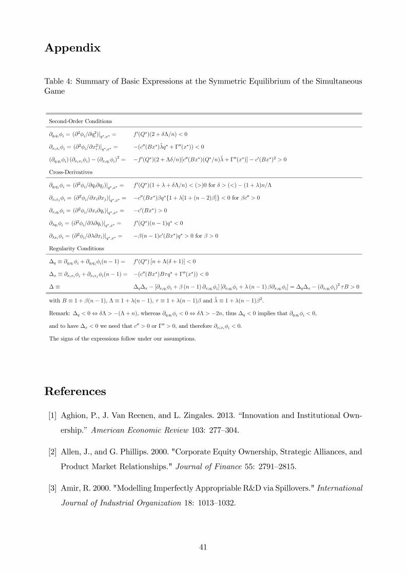
Appendix

Table 4: Summary of Basic Expressions at the Symmetric Equilibrium of the SimultaneousGame

Second-Order Conditions

@qiqi�i = (@2�i=@q2i )jq�;x� = f 0(Q�)(2 + ��=n) < 0

@xixi�i = (@2�i=@x2i )jq�;x� = �(c00(Bx�)~�q� + �00(x�)) < 0

(@qiqi�i) (@xixi�i)� (@xiqi�i)2 = �f 0(Q�)(2 + ��=n)[c00(Bx�)(Q�=n)~�+ �00(x�)]� c0(Bx�)2 > 0

Cross-Derivatives

@qiqj�i = (@2�i=@qi@qj)jq�;x� = f 0(Q�)(1 + �+ ��=n) < (>)0 for � > (<)� (1 + �)n=�

@xixj�i = (@2�i=@xi@xj)jq�;x� = �c00(Bx�)�q�f1 + �[1 + (n� 2)�]g < 0 for �c00 > 0

@xiqi�i = (@2�i=@xi@qi)jq�;x� = �c0(Bx�) > 0

@�qi�i = (@2�i=@�@qi)jq�;x� = f 0(Q�)(n� 1)q� < 0

@�xi�i = (@2�i=@�@xi)jq�;x� = ��(n� 1)c0(Bx�)q� > 0 for � > 0

Regularity Conditions

�q � @qiqi�i + @qiqj�i(n� 1) = f 0(Q�) [n+ �(� + 1)] < 0

�x � @xixi�i + @xixj�i(n� 1) = �(c00(Bx�)B�q� + �00(x�)) < 0

� � �q�x � [@xiqi�i + � (n� 1) @xiqi�i] [@xiqi�i + � (n� 1) �@xiqi�i] = �q�x � (@xiqi�i)2 �B > 0

with B � 1 + �(n� 1), � � 1 + �(n� 1), � � 1 + �(n� 1)� and ~� � 1 + �(n� 1)�2.

Remark: �q < 0, �� > �(� + n), whereas @qiqi�i < 0, �� > �2n, thus �q < 0 implies that @qiqi�i < 0,

and to have �x < 0 we need that c00 > 0 or �00 > 0, and therefore @xixi�i < 0.

The signs of the expressions follow under our assumptions.

References

[1] Aghion, P., J. Van Reenen, and L. Zingales. 2013. �Innovation and Institutional Own-

ership.�American Economic Review 103: 277�304.

[2] Allen, J., and G. Phillips. 2000. "Corporate Equity Ownership, Strategic Alliances, and

Product Market Relationships." Journal of Finance 55: 2791�2815.

[3] Amir, R. 2000. "Modelling Imperfectly Appropriable R&D via Spillovers." International

Journal of Industrial Organization 18: 1013�1032.

41

[4] Anton, M., F. Ederer, M. Giné, and M. Schmalz. 2017. �Common Ownership, Com-

petition, and Top Management Incentives.� Ross School of Business working paper

1328.

[5] Azar, J., S. Raina, and M.C. Schmalz. 2016. "Ultimate Ownership and Bank Compe-

tition." Available at SSRN.

[6] Azar, J., M.C. Schmalz, and I. Tecu. (forthcoming). "Anti-competitive E¤ects of Com-

mon Ownership." Journal of Finance.

[7] Baker, J. 2016. "Overlapping Financial Investor Ownership, Market Power, and An-

titrust Enforcement: My Quali�ed Agreement with Professor Elhauge." Harvard Law

Review 129: 212�232.

[8] Banal-Estanol, A., J. Seldeslachts, and X. Vives. 2018. "Common Ownership -Product

Market Consequences of a Shift from Active to Passive Investors." Mimeo.

[9] Besanko, D., and D.F. Spulber. 1989. "Antitrust Enforcement under Asymmetric In-

formation." Economic Journal 99: 408�25.

[10] Bloom, N., M. Schankerman, and J. Van Reenen. 2013. "Identifying Technology

Spillovers and Product Market Rivalry." Econometrica 81: 1347�1393.

[11] Blume, M.E., and B. Keim. 2014. "The Changing Nature of Institutional Stock Invest-

ing". Working paper.

[12] Bresnahan, T.F., S.C. Salop. 1986. "Quantifying the Competitive E¤ects of Production

Joint Ventures." International Journal of Industrial Organization 4: 155�175.

[13] Brito, D., R. Ribeiro, and H. Vasconcelos. 2014. �Measuring Unilateral E¤ects in Partial

Horizontal Acquisitions,�International Journal of Industrial Organization 33: 22�36.

[14] Brito, D., Osório, A., Ribeiro, R., and H. Vasconcelos. (forthcoming). "Unilateral Ef-

fects Screens for Partial Horizontal Acquisitions: The Generalized HHI and GUPPI."

International Journal of Industrial Organization.

[15] Brodley, J. 1990. "Antitrust Law and Innovation Cooperation." Journal of Economic

Perspectives 4: 97�112.

42

[16] Bulow, J., and P. P�eiderer. 1983. �A Note on the E¤ect of Cost Changes on Prices.�

Journal of Political Economy 91: 182�185.

[17] Bushee, B. 1998. "The In�uence of Institutional Investors on Myopic R&D Investment

Behavior." The Accounting Review 73:305�333.

[18] Cabral, L. 2000. "R&D Cooperation and Product Market Competition." International

Journal of Industrial Organization 18: 1033�1047.

[19] CEA. 2016. "Bene�ts of Competition and Indicators of Market Power." Council of

Economic Advisers Issue Brief. April.

[20] Dasgupta, P., and J. Stiglitz. 1980. "Industrial Structure and the Nature of Innovative

Activity." Economic Journal 90: 266�93.

[21] d�Aspremont, C., and A. Jacquemin. 1988. "Cooperative and Noncooperative R&D in

Duopoly with Spillovers." The American Economic Review 78: 1133�1137.

[22] De Loecker, J., and J. Eeckhout. 2017. "The Rise of Market Power and the Macroeco-

nomic Implications". Working paper.

[23] Dietzenbacher, E., B. Smid, and B. Volkerink. 2000. �Horizontal Integration in the

Dutch Financial Sector,� International Journal of Industrial Organization 18: 1223�

1242.

[24] Dixit, A., and J. Stiglitz. 1977. �Monopolistic Competition and Optimum Product

Diversity.�American Economic Review 67: 297�308.

[25] Dixit, A. 1986. �Comparative Statics for Oligopoly.� International Economic Review

27: 107�122.

[26] Duso, T., L-H. Röller, and J. Seldeslachts. 2014. "Collusion Through Joint R&D: An

Empirical Assessment." The Review of Economics and Statistics 96: 349�370.

[27] Edgeworth, F. Y. 1881. Mathematical Physics: An Essay on the Application of Mathe-

matics to the Moral Sciences. (Kegan Paul, London).

[28] Elhauge, E. 2016. "Horizontal Shareholding." Harvard Law Review 109: 1267�1317.

43

[29] Elhauge E. 2017. "Tackling horizontal shareholding: an update and extension to the

Sherman Act and EU competition law." Background Paper for 128th meeting of the

OECD Competition Committee.

[30] Eng, L.L., and M. Shackell. 2001. "The Implications of Long-Term Performance Plans

and Institutional Ownership for Firms�Research and Development (R/D&D) Invest-

ments." Journal of Accounting, Auditing & Finance 16: 117�139.

[31] European Commission [EC]. 2014. "White Paper: Towards More E¤ective EU Merger

Control." Brussels, 9.7.2014. COM(2014) 449 �nal.

[32] European Commission[EC] Decision.2017. Case M.7392, Dow/Dupont, 27 march.

[33] Farrell, J., and C. Shapiro. 1990. "Asset Ownership and Market Structure in Oligopoly."

RAND Journal of Economics 21: 275�292.

[34] Fee, C. E., C. J. Hadlock, and S. Thomas. 2006. "Corporate Equity Ownership and the

Governance of Product Market Relationships." Journal of Finance 61:1217�1251.

[35] Flath, D. 1991. "When is it Rational for Firms to Acquire Silent Interests in Rivals?"

International Journal of Industrial Organization 9: 573�584.

[36] Fudenberg, D., and J. Tirole. 1984. �The Fat-Cat E¤ect, the Puppy-Dog Ploy, and the

Lean and Hungry Look.�The American Economic Review 74: 361�366.

[37] Galasso, A., and M. Schankerman. 2015. "Patents and Cumulative Innovation: Causal

Evidence from the Courts." Quarterly Journal of Economics 130: 317�369.

[38] Geng, H., H. Hau, and S. Lai. 2016. "Technological Progress and Ownership Structure."

SFI research paper series 15�39.

[39] Ghosh, A., and H. Morita. 2017. "Knowledge Transfer and Partial Equity Ownership."

Rand Journal of Economics 48: 1044�1067.

[40] Gilbert, R. 2006. Looking for Mr. Schumpeter: Where Are We in the Competition-

Innovation Debate?, in Adam B. Ja¤e, Josh Lerner and Scott Stern (eds), Innovation

Policy and the Economy 6: 159�215. The MIT Press.

[41] Gilbert, R., and H. Greene. 2015. "Merging Innovation into Antitrust Agency Enforce-

ment of the Clayton Act." The George Washington Law Review 83: 1919�1947.

44

[42] Gilo, D. 2000. "The Anticompetitive E¤ect of Passive Investment." Michigan Law Re-

view 99: 1�47.

[43] Gilo, D., Y. Moshe, and Y. Spiegel. 2006. "Partial Cross Ownership and Tacit Collu-

sion." RAND Journal of Economics 37: 81�99.

[44] Goeree, M., and E. Helland. 2010. "Do Research Joint Ventures Serve a Collusive

Function?" Working Paper 448, Institute for Empirical Research in Economics.

[45] Gramlich, J., and Grundl, S. 2017. "Estimating the Competitive E¤ects of Common

Ownership." Mimeo.

[46] Greenlee, P., and B. Cassiman. 1999. "Product Market Objectives and the Formation

of Research Joint Ventures." Managerial and Decision Economics 20: 115�130.

[47] Griliches, Z. 1990. "Patent Statistics as Economic Indicators: A Survey." Journal of

Economic Literature 28: 1661�1707.

[48] Grossman, M., and C. Shapiro. 1986. "Research Joint Ventures: An Antitrust Analy-

sis." Journal of Law, Economics, & Organization 2: 315�337.

[49] Grullon, G., Y. Larkin, and R. Michaely. 2017. "Are US Industries Becoming More

Concentrated". Mimeo.

[50] Gutiérrez, G. and T. Philippon. 2016. "Investment-less Growth: An Empirical Investi-

gation." Mimeo.

[51] Hansen R. and J. Lott, Jr. 1996. "Externalities and corporate objectives in a world

with diversi�ed shareholder/consumers." Journal of Financial and Quantitative Analy-

sis 31:43�68.

[52] He, J.J., and J. Huang. 2017. "Product Market Competition in a World of Cross Own-

ership: Evidence from Institutional Blockholdings." Review of Financial Studies 30:

2674�2718.

[53] Heim, M., K. Hüschelrath, and Y. Spiegel. 2017. �Minority Share Acquisitions and

Collusion: Evidence from the Introduction of National Leniency Programs.�Mimeo.

45

[54] Investment Company Institute. 2017. Fact Book - A Review of Trends and Activities

in the Investment Company Industry. Retrieved from Investment Company Institute

Website: https://www.ici.org/pdf/2017_factbook.pdf

[55] Kamien, M., E. Muller, and I. Zang. 1992. "Research Joint Ventures and R&D Cartels."

The American Economic Review 82: 1293�1306.

[56] Karle, H., T.J. Klein, and K. Stahl. 2011. "Ownership and Control in a Competitive

Industry." CESifo Working Paper No. 3380.

[57] Kennedy, P., D. O�Brien, M. Song, and K. Whaerer. 2017. "The Competitive E¤ects of

Common Ownership: Economic Foundations and Empirical Evidence." Mimeo.

[58] Lambertini, L., S., Poddar and D. Sasaki. 2002. "Research Joint Ventures, Product

Di¤erentiation and Price Collusion." International Journal of Industrial Organization

20: 829�854.

[59] Leahy, D., and P. Neary. 1997. "Public Policy towards R&D in Oligopolistic Industries."

The American Economic Review 87: 642�662.

[60] Liang, L. M. 2016. "Common Ownership and Executive Compensation." Mimeo.

[61] Martin, S. 1995. "R&D Joint Ventures and Tacit Product Market Collusion." European

Journal of Political Economy 11: 733�741.

[62] Michel, C. 2016. "Identi�cation and Estimation of Intra-Firm and Industry Competition

via Ownership Change." Mimeo.

[63] Miyagiwa, K. 2009. "Collusion and Research Joint Ventures." The Journal of Industrial

Economics 57: 768�784.

[64] Nain, A., and Y. Wang. 2016. �The Product Market Impact of Minority Stake Acqui-

sitions,�Management Science 64: 825�844.

[65] Norbäck, P-J., Persson, L. and Tag, J. 2018. �Private Equity Buyouts: Anti-or Pro-

competitive?�Antitrust Chronicle 1: 32�36.

[66] Parker, P. M., and L-H. Röller. 1997. "Collusive Conduct in Duopolies: Multimarket

Contact and Cross-Ownership in the Mobile Telephone Industry." Rand Journal of

Economics 28: 304-322.

46

[67] Posner, E., F. Scott Morton, and E. G. Weyl. 2016. "A Proposal to Limit the Anti-

Competitive Power of Institutional Investors." Mimeo.

[68] Reitman, D. 1994. "Partial Ownership Arrangements and the Potential for Collusion."

The Journal of Industrial Economics 42: 313�322.

[69] Reynolds, R.J., B.R. Snapp. 1986. "The Competitive E¤ects of Partial Equity Interests

and Joint Ventures." International Journal of Industrial Organization 4: 141�153.

[70] Rock, E. B., and D. L. Rubinfeld. 2017. "Antitrust for Institutional Investors." NYU

School of Law, WP NO.17�23.

[71] Salop, S.C., and D.P. O�Brien. 2000. "Competitive E¤ects of Partial Ownership: Fi-

nancial Interest and Corporate Control." Antitrust Law Journal 67: 559�614.

[72] Schmalz, M.C. 2018. "Common-Ownership Concentration and Corporate Conduct."

Annual Review of Financial Economics 10: 1�31.

[73] Shelegia, S., and Y. Spiegel. 2012. "Bertrand Competition when Firms Hold Passive

Ownership Stakes in One Another." Economics Letters 114: 136�138.

[74] Spence, M. 1984. "Cost Reduction, Competition and Industry Performance." Econo-

metrica 52: 101�121.

[75] Suetens, S. 2008. "Does R&D Cooperation Facilitate Price Collusion? An Experiment."

Journal of Economic Behavior & Organization 66: 822�836.

[76] Sullivan, J. 2016. "The Ice Cream Split: Empirically Distinguishing Price and Product

Space Collusion." Mimeo.

[77] Vives, X. 1999. Oligopoly Pricing: Old Ideas and New Tools. Cambridge, MA: MIT

Press.

[78] Vives, X. 2008. "Innovation and Competitive Pressure." The Journal of Industrial Eco-

nomics 56: 419�469.

[79] Vonortas, N.S. 2000. "Multimarket Contact and Inter-Firm Cooperation in R&D."

Journal of Evolutionary Economics 10: 243�271.

[80] Weyl, E.G., and M. Fabinger. 2013. "Pass-Through as an Economic Tool: Principles of

Incidence under Imperfect Competition." Journal of Political Economy 121: 528�583.

47

[81] Wilkinson, L.A., and J.L. White. 2007. "Private Equity: Antitrust Concerns with Par-

tial Acquisitions." Antitrust 21: 28�34.

48

Online appendix to Overlapping Ownership, R&D Spillovers

and Antitrust Policy

Ángel L. López and Xavier Vives

July 2018

Contents

A Proofs and the three model speci�cations 2

A.1 General model: proofs . . . . . . . . . . . . . . . . . . . . . . . . . . . . . . . . . 2

A.1.1 Overlapping ownership and � . . . . . . . . . . . . . . . . . . . . . . . . . 2

A.1.2 Simultaneous model . . . . . . . . . . . . . . . . . . . . . . . . . . . . . . 5

A.1.3 Two-stage model . . . . . . . . . . . . . . . . . . . . . . . . . . . . . . . . 13

A.2 The three model speci�cations . . . . . . . . . . . . . . . . . . . . . . . . . . . . 17

A.2.1 Simultaneous model . . . . . . . . . . . . . . . . . . . . . . . . . . . . . . 18

A.2.2 Two-stage model . . . . . . . . . . . . . . . . . . . . . . . . . . . . . . . . 30

B Bertrand competition with di¤erentiated products 37

B.1 Framework and equilibrium . . . . . . . . . . . . . . . . . . . . . . . . . . . . . . 37

B.2 Simultaneous model . . . . . . . . . . . . . . . . . . . . . . . . . . . . . . . . . . 38

B.2.1 Comparative statics with respect to � . . . . . . . . . . . . . . . . . . . . 39

B.2.2 Welfare analysis . . . . . . . . . . . . . . . . . . . . . . . . . . . . . . . . 44

B.3 Two-stage model . . . . . . . . . . . . . . . . . . . . . . . . . . . . . . . . . . . . 45

B.4 Model speci�cations . . . . . . . . . . . . . . . . . . . . . . . . . . . . . . . . . . 49

B.4.1 Linear model . . . . . . . . . . . . . . . . . . . . . . . . . . . . . . . . . . 49

B.4.2 Constant elasticity model . . . . . . . . . . . . . . . . . . . . . . . . . . . 66

In Appendix A we provide some technical details and proofs of results in the paper in Section

A.1, and analysis and results for the three model speci�cations in Section A.2. In Appendix B

we develop the Bertrand model with product di¤erentiation.

1

A Proofs and the three model speci�cations

A.1 General model: proofs

A.1.1 Overlapping ownership and �

Common ownership Consider an industry with n �rms and I � n investors; we let i and

j index (respectively) investors and �rms. The share of �rm j owned by investor i is �ij , and

the parameter �ij captures the extent of i�s control over �rm j. The total (portfolio) pro�t of

investor i is �i =Pk �ik�k, where �k are the pro�ts of portfolio �rm k. The manager of �rm j

takes into account shareholders�incentives (through the control weights �ij) and maximizes a

weighted average of the shareholders�portfolio pro�ts:

IXi=1

�ij�i =

IXi=1

�ij�ij

!�j +

IXi=1

�ij

nXk 6=j

�ik�k:

It is immediate dividing byPIi=1 �ij�ij that the objective of the manager can be rewritten as

�j = �j +nXk 6=j

�jk�k, where �jk �PIi=1 �ij�ikPIi=1 �ij�ij

:

The parameter �jk is the relative weight that the manager of �rm j places on the pro�t of

�rm k in relation to the own pro�t (of �rm j) and re�ects the control of �rm j by investors

with �nancial interests in �rms j and k. For the manager of �rm j to put weight on the interest

of investor i we need �ij�ik > 0: investor i has to have a stake in �rm k (�ik > 0) and some

control over �rm j (�ij > 0). The weight �jk is larger the more �rm j is controlled (high �ij)

by investors with high stakes in �rm k (high �ik) and the less concentrated the ownership and

control of �rm j (low denominatorPIi=1 �ij�ij). The numerator

PIi=1 �ij�ik is a measure of

the ownership concentration and control of �rm k. As the ratio �jk increases, the in�uence of

the common owners of �rm k over the manager of �rm j increases.

We next discuss the cases of silent �nancial interests and proportional control. In both cases

we assume that each �rm has a reference shareholder and each investor acquires a share � of the

�rms which are not under his control. The reference shareholder keeps an interest 1� (I � 1)�

in his �rm and we assume that �I < 1 so that 1� (I � 1)� > �.

Silent Financial Interest (SFI). In this case, each owner (i.e., the majority or dominant

shareholder) i retains full control of the acquiring �rm and is entitled to a share � of the acquired

�rms�pro�ts� but exerts no in�uence over the latter�s decisions. Then �SFI = �= [1� (I � 1)�]

is just the ratio of the share on an acquired �rm k (�ik = � in k, numerator of �jk) over

2

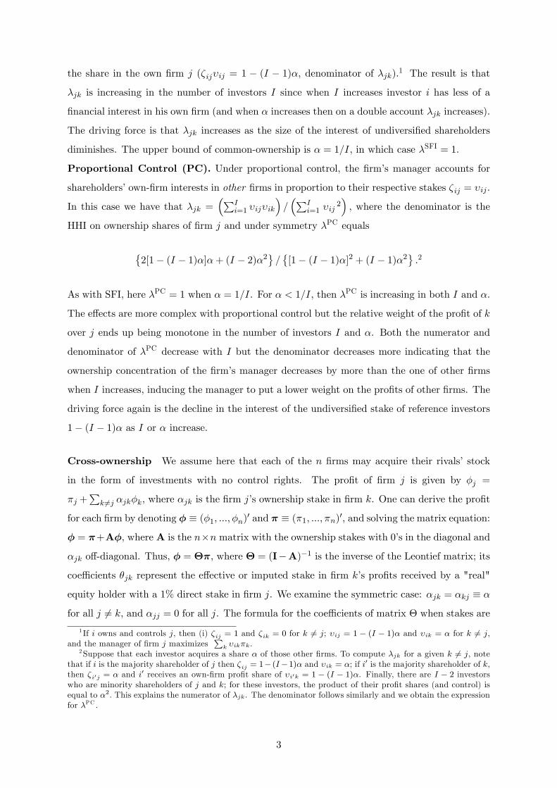
the share in the own �rm j (�ij�ij = 1 � (I � 1)�, denominator of �jk).1 The result is that

�jk is increasing in the number of investors I since when I increases investor i has less of a

�nancial interest in his own �rm (and when � increases then on a double account �jk increases).

The driving force is that �jk increases as the size of the interest of undiversi�ed shareholders

diminishes. The upper bound of common-ownership is � = 1=I, in which case �SFI = 1.

Proportional Control (PC). Under proportional control, the �rm�s manager accounts for

shareholders�own-�rm interests in other �rms in proportion to their respective stakes �ij = �ij .

In this case we have that �jk =�PI

i=1 �ij�ik

�=�PI

i=1 �ij2�; where the denominator is the

HHI on ownership shares of �rm j and under symmetry �PC equals

�2[1� (I � 1)�]�+ (I � 2)�2

=�[1� (I � 1)�]2 + (I � 1)�2

:2

As with SFI, here �PC = 1 when � = 1=I. For � < 1=I, then �PC is increasing in both I and �.

The e¤ects are more complex with proportional control but the relative weight of the pro�t of k

over j ends up being monotone in the number of investors I and �. Both the numerator and

denominator of �PC decrease with I but the denominator decreases more indicating that the

ownership concentration of the �rm�s manager decreases by more than the one of other �rms

when I increases, inducing the manager to put a lower weight on the pro�ts of other �rms. The

driving force again is the decline in the interest of the undiversi�ed stake of reference investors

1� (I � 1)� as I or � increase.

Cross-ownership We assume here that each of the n �rms may acquire their rivals�stock

in the form of investments with no control rights. The pro�t of �rm j is given by �j =

�j +Pk 6=j �jk�k, where �jk is the �rm j�s ownership stake in �rm k. One can derive the pro�t

for each �rm by denoting � � (�1; :::; �n)0 and � � (�1; :::; �n)0, and solving the matrix equation:

� = �+A�, where A is the n�n matrix with the ownership stakes with 0�s in the diagonal and

�jk o¤-diagonal. Thus, � = ��, where � = (I�A)�1 is the inverse of the Leontief matrix; its

coe¢ cients �jk represent the e¤ective or imputed stake in �rm k�s pro�ts received by a "real"

equity holder with a 1% direct stake in �rm j. We examine the symmetric case: �jk = �kj � �

for all j 6= k, and �jj = 0 for all j. The formula for the coe¢ cients of matrix � when stakes are

1 If i owns and controls j, then (i) �ij = 1 and �ik = 0 for k 6= j; �ij = 1 � (I � 1)� and �ik = � for k 6= j,and the manager of �rm j maximizes

Pk �ik�k.

2Suppose that each investor acquires a share � of those other �rms. To compute �jk for a given k 6= j, notethat if i is the majority shareholder of j then �ij = 1� (I�1)� and �ik = �; if i0 is the majority shareholder of k,then �i0j = � and i0 receives an own-�rm pro�t share of �i0k = 1 � (I � 1)�. Finally, there are I � 2 investorswho are minority shareholders of j and k; for these investors, the product of their pro�t shares (and control) isequal to �2. This explains the numerator of �jk. The denominator follows similarly and we obtain the expressionfor �PC :

3

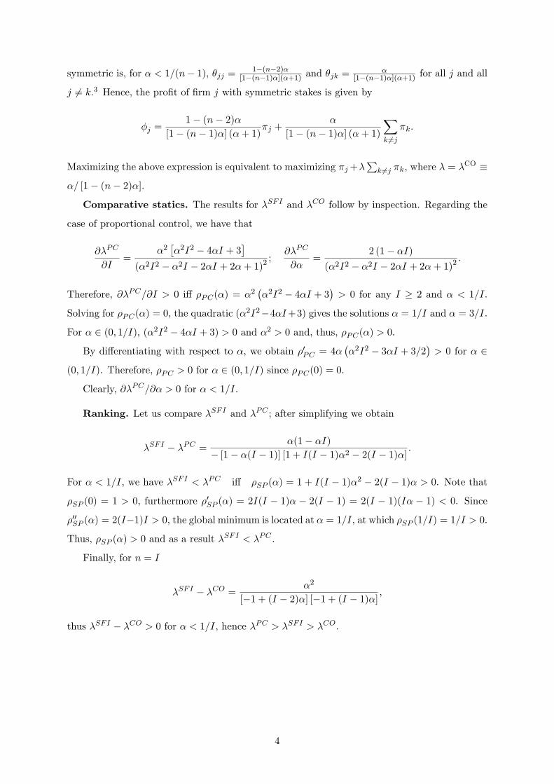
symmetric is, for � < 1=(n� 1), �jj = 1�(n�2)�[1�(n�1)�](�+1) and �jk =

�[1�(n�1)�](�+1) for all j and all

j 6= k.3 Hence, the pro�t of �rm j with symmetric stakes is given by

�j =1� (n� 2)�

[1� (n� 1)�] (�+ 1)�j +�

[1� (n� 1)�] (�+ 1)Xk 6=j

�k:

Maximizing the above expression is equivalent to maximizing �j+�Pk 6=j �k, where � = �CO �

�= [1� (n� 2)�].

Comparative statics. The results for �SFI and �CO follow by inspection. Regarding the

case of proportional control, we have that

@�PC

@I=

�2��2I2 � 4�I + 3

�(�2I2 � �2I � 2�I + 2�+ 1)2

;@�PC

@�=

2 (1� �I)(�2I2 � �2I � 2�I + 2�+ 1)2

.

Therefore, @�PC=@I > 0 i¤ �PC(�) = �2��2I2 � 4�I + 3

�> 0 for any I � 2 and � < 1=I.

Solving for �PC(�) = 0, the quadratic (�2I2�4�I+3) gives the solutions � = 1=I and � = 3=I.

For � 2 (0; 1=I), (�2I2 � 4�I + 3) > 0 and �2 > 0 and, thus, �PC(�) > 0.

By di¤erentiating with respect to �, we obtain �0PC = 4���2I2 � 3�I + 3=2

�> 0 for � 2

(0; 1=I). Therefore, �PC > 0 for � 2 (0; 1=I) since �PC(0) = 0.

Clearly, @�PC=@� > 0 for � < 1=I.

Ranking. Let us compare �SFI and �PC ; after simplifying we obtain

�SFI � �PC = �(1� �I)� [1� �(I � 1)] [1 + I(I � 1)�2 � 2(I � 1)�] .

For � < 1=I, we have �SFI < �PC i¤ �SP (�) = 1 + I(I � 1)�2 � 2(I � 1)� > 0. Note that

�SP (0) = 1 > 0, furthermore �0SP (�) = 2I(I � 1)� � 2(I � 1) = 2(I � 1)(I� � 1) < 0. Since

�00SP (�) = 2(I�1)I > 0, the global minimum is located at � = 1=I, at which �SP (1=I) = 1=I > 0.

Thus, �SP (�) > 0 and as a result �SFI < �PC .

Finally, for n = I

�SFI � �CO = �2

[�1 + (I � 2)�] [�1 + (I � 1)�] ,

thus �SFI � �CO > 0 for � < 1=I, hence �PC > �SFI > �CO.

4

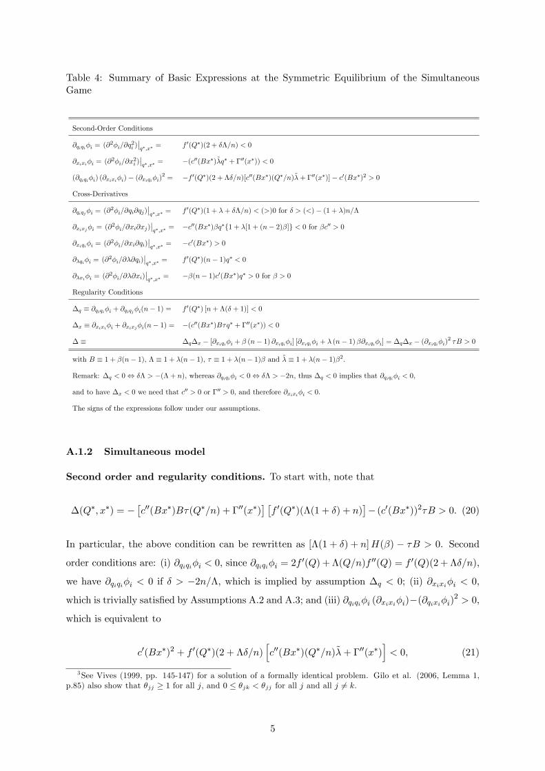
Table 4: Summary of Basic Expressions at the Symmetric Equilibrium of the SimultaneousGame

Second-Order Conditions

@qiqi�i = (@2�i=@q2i )��q�;x�

= f 0(Q�)(2 + ��=n) < 0

@xixi�i = (@2�i=@x2i )��q�;x�

= �(c00(Bx�)~�q� + �00(x�)) < 0

(@qiqi�i) (@xixi�i)� (@xiqi�i)2 = �f 0(Q�)(2 + ��=n)[c00(Bx�)(Q�=n)~�+ �00(x�)]� c0(Bx�)2 > 0

Cross-Derivatives

@qiqj�i = (@2�i=@qi@qj)��q�;x�

= f 0(Q�)(1 + �+ ��=n) < (>)0 for � > (<)� (1 + �)n=�

@xixj�i = (@2�i=@xi@xj)��q�;x�

= �c00(Bx�)�q�f1 + �[1 + (n� 2)�]g < 0 for �c00 > 0

@xiqi�i = (@2�i=@xi@qi)��q�;x�

= �c0(Bx�) > 0

@�qi�i = (@2�i=@�@qi)��q�;x�

= f 0(Q�)(n� 1)q� < 0

@�xi�i = (@2�i=@�@xi)��q�;x�

= ��(n� 1)c0(Bx�)q� > 0 for � > 0

Regularity Conditions

�q � @qiqi�i + @qiqj�i(n� 1) = f 0(Q�) [n+ �(� + 1)] < 0

�x � @xixi�i + @xixj�i(n� 1) = �(c00(Bx�)B�q� + �00(x�)) < 0

� � �q�x � [@xiqi�i + � (n� 1) @xiqi�i] [@xiqi�i + � (n� 1)�@xiqi�i] = �q�x � (@xiqi�i)2 �B > 0

with B � 1 + �(n� 1), � � 1 + �(n� 1), � � 1 + �(n� 1)� and ~� � 1 + �(n� 1)�2.

Remark: �q < 0, �� > �(� + n), whereas @qiqi�i < 0, �� > �2n, thus �q < 0 implies that @qiqi�i < 0,

and to have �x < 0 we need that c00 > 0 or �00 > 0, and therefore @xixi�i < 0.

The signs of the expressions follow under our assumptions.

A.1.2 Simultaneous model

Second order and regularity conditions. To start with, note that

�(Q�; x�) = ��c00(Bx�)B�(Q�=n) + �00(x�)

� �f 0(Q�)(�(1 + �) + n)

�� (c0(Bx�))2�B > 0. (20)

In particular, the above condition can be rewritten as [�(1 + �) + n]H(�) � �B > 0. Second

order conditions are: (i) @qiqi�i < 0, since @qiqi�i = 2f0(Q) + �(Q=n)f 00(Q) = f 0(Q)(2 + ��=n),

we have @qiqi�i < 0 if � > �2n=�, which is implied by assumption �q < 0; (ii) @xixi�i < 0,

which is trivially satis�ed by Assumptions A.2 and A.3; and (iii) @qiqi�i (@xixi�i)�(@qixi�i)2 > 0,

which is equivalent to

c0(Bx�)2 + f 0(Q�)(2 + ��=n)hc00(Bx�)(Q�=n)~�+ �00(x�)

i< 0, (21)

3See Vives (1999, pp. 145-147) for a solution of a formally identical problem. Gilo et al. (2006, Lemma 1,p.85) also show that �jj � 1 for all j, and 0 � �jk < �jj for all j and all j 6= k.

5

where ~� = 1 + �(n� 1)�2. Noting that @qiqj�i = f 0(Q�)(1 + �) + f 00(Q�)�q� = f 0(Q�)(1 + �+

��=n), we have that

�q � @qiqi�i + @qiqj�i(n� 1) = f 0(Q�) [n+ �(� + 1)] < 0,

which is satis�ed if � > �(n + �)=�. Similarly, noting that @xixi�i = �c00(Bx�)~�q� � �00(x�)

and @xixj�i = �c00(Bx�)�q� f1 + � [1 + (n� 2)�]g, it is straightforward to show that

�x � @xixi�i + @xixj�i(n� 1) = ��c00(Bx�)B�q� + �00(x�)

�< 0,

which is satis�ed by Assumptions A.2 and A.3.

Proof of Lemma 1. Using equation (6) and Table 4 we obtain

@x�

@�=c0(Bx�)f 0(Q�)(n� 1)q�

�f� [�(1 + �) + n]� �g :

Since � > 0,

sign

�@x�

@�

�= sign f� [� (1 + �) + n]� �g

= sign

�� � �

� (1 + �) + n

�= sign

n� � P 0(c) �

n

o;

where P 0(c) = n=[�(1+�)+n]. Note that �(1+�)+n > 0 since �q < 0. Finally, by substituting

sign f� [� (1 + �) + n]� �g = sign f�(1 + n+ ��)� 1g :�

Proof of Corollary 1. From Lemma 1 we have that if � � �(1+n)=�, so 1+n+ �� � 0,

then @x�=@� < 0, which, using equation (7), in turn implies that @q�=@� < 0: for all � only

RI exists. If � > �(n + 1)=�, then in addition to RI, region RII exists only if � > �n=� also

holds. The reason is that when 1 + n + �� > 0, then, from Lemma 1, @x�=@� > 0 requires

that � > 1=(1 + n + ��). However, 1=(1 + n + ��) < 1 only if � > �n=�, in which case there

exists some region of feasible spillover values for which @x�=@� > 0. Note that for a given n,

the condition � > �n=� is stricter than the condition � > �(n + 1)=�. Thus, for � � �n=�

only RI exists, and since �n=� increases with �, the result holds for any � if � � �n.�

6

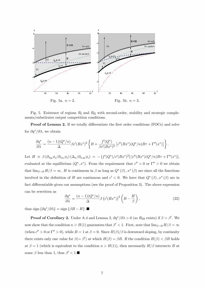
Fig. 5a. n = 2. Fig. 5b. n = 3.

Fig. 5. Existence of regions RI and RII with second-order, stability and strategic comple-ments/substitutes output competition conditions.

Proof of Lemma 2. If we totally di¤erentiate the �rst order conditions (FOCs) and solve

for @q�=@�, we obtain

@q�

@�=(n� 1)(Q�=n)

��c0(Bx�)2

�B +

f 0(Q�)

�c0(Bx�)2�c00(Bx�)(Q�=n)B� + �00(x�)

��:

Let H � � (@�qi�i=@�xi�i) (�x=@xiqi�i) = ��f 0(Q�)=c0(Bx�)2

�[c00(Bx�)(Q�=n)B� + �00(x�)],

evaluated at the equilibrium (Q�; x�). From the requirement that c00 > 0 or �00 > 0 we obtain

that lim�!0H=� =1. H is continuous in � as long as Q� (�) ; x� (�) are since all the functions

involved in the de�nition of H are continuous and c0 < 0. We have that Q� (�) ; x� (�) are in

fact di¤erentiable given our assumptions (see the proof of Proposition 3). The above expression

can be rewritten as@q�

@�=(n� 1)(Q�=n)

���c0(Bx�)

�2�B � H

�

�; (22)

thus sign f@q�=@�g = sign f�B �Hg :�

Proof of Corollary 2. Under A.4 and Lemma 2, @q�=@� > 0 (so RIII exists) if � > �0. We

now show that the condition n > H(1) guarantees that �0 < 1. First, note that lim�!0H=� =1

(when c00 > 0 or �00 > 0), whileB = 1 at � = 0. SinceH(�)=� is downward sloping, by continuity

there exists only one value for �(= �0) at which H(�) = �B. If the condition H(�) < �B holds

at � = 1 (which is equivalent to the condition n > H(1)), then necessarily H=� intersects B at

some � less than 1, thus �0 < 1.�

7

Proof of Proposition 2. Pro�t per �rm as a function of � at equilibrium is given by

��(�) = (f(Q�)� c(Bx�)) q� � �(x�).

By di¤erentiating �� with respect to �, we obtain

��0(�) = f 0(Q�)n@q�

@�q� � c0(Bx�)B@x

�

@�q� + (f(Q�)� c(Bx�)) @q

�

@�� �0(x�)@x

�

@�.

Using that in equilibrium f(Q�) � c(Bx�) = �f 0(Q�)�q� and �0(x�) = �c0(Bx�)q�� , we can

rewrite the above expression as

��0(�) = f 0(Q�)n@q�

@�q� � c0(Bx�)B@x

�

@�q� � f 0(Q�)�q�@q

�

@�+ c0(Bx�)q��

@x�

@�

= f 0(Q�)(n� �)q�@q�

@�+ c0(Bx�)(� �B)q�@x

�

@�

= (n� 1)(1� �)q��f 0(Q�)

@q�

@�� �c0(Bx�)@x

�

@�

�.

In RII, we have that @x�=@� > 0 and @q�=@� < 0. Hence from the above expression it is clear

that ��0(�) > 0. Note also that when � = 0, the equilibrium is in RI, and therefore ��0(�) > 0

since @q�=@� < 0. To determine signf��0(�)g in RI and RIII for � > 0, we replace @q�=@� and

@x�=@� with the expressions derived in the proofs of Lemmata 1, 2:

��0(�) = (n� 1)(1� �)q��f 0(Q�)

(n� 1)q��

c0(Bx�)2�

�B � H(�)

�

���c0(Bx�)(n� 1)q

�

�f 0(Q�)c0(Bx�) f� [�(1 + �) + n]� �g

�= #�

�� [�(1 + �) + n]� � + H(�)

��B

�,

where #� � (n� 1)(1� �)q� [(n� 1)q�=�] c0(Bx�)2�(�f 0(Q�)) is positive. Therefore,

sign���0(�)

= sign

�(n+ 1 + ��)� � 1 + H(�)

��B

�, (23)

so it follows that ��0(�) > 0 if

1� (n+ 1 + ��)� < H(�)

��B, or equivalently (24)

2(1� �)� ��� < H(�)

�. (25)

From Table 4 and using that in equilibrium �q� = ��0(x�)=c0(Bx�), the regularity condition

8

can be written as

���c00(Bx�)B �0(x�)

c0(Bx�)+ �00(x�)

�f 0(Q�)

c0(Bx�)2[� (1 + �) + n]� �B > 0.

Noting that

H(�) =�f 0(Q�)c0(Bx�)2

��c

00(Bx�)

c0(Bx�)B�0(x�) + �00(x�)

�,

we can rewrite the regularity condition in terms of H as follows: [�(1 + �) + n]H(�)� �B > 0,

with �(1 + �) + n > 0 since �q < 0. Thus, if the equilibrium is regular:

H(�)

�>

�B

[�(1 + �) + n]�.

Then, we only have to show that:

~g(�) � �B > ~h(�) � [2(1� �)� ���][�(1 + �) + n]�

holds. Note that ~g(0) = 1, ~g0(�) > 0, ~g00(�) > 0 for � > 0 and ~g00(0) = 0. On the other hand,

~h(0) = 0 and

~h0(�) = 2[�(1 + �) + n][1� (2 + ��)�].

Furthermore, it can be shown that solving the equation ~g(�) = ~h(�) for � yields the following

two roots:

�1 =1

�� + n+ 1and �2 =

1

�(� + 1) + 1.

Consider RI. If the smallest (positive) root in this region is larger or equal to the spillover

threshold � that determines RI (i.e. for � < �, @x�

@� < 0 for all �), then ~g(�) > ~h(�) in RI, and

consequently, ��0(�) > 0. First, note that when �� + n + 1 > 0, �1 = �. We distinguish the

following cases:

� If �� + n + 1 > 0, then: if �(� + 1) + 1 > 0, (for � < 1) �2 > �1 = � > 0, while

if �(� + 1) + 1 < 0, �1 = � > 0 > �2, so in any case �1 = � is the smallest positive

root in the region and, thus, ~g(�) > ~h(�) for � 2 (0; �1). Also, in any case for � = �1,

@x�=@� = 0 and so signf��0(�)g = signff 0(Q�)@q�=@�g, which is positive in RI since in

this region: @q�=@� < 0.

� If �� + n+ 1 < 0, then 0 > �1 > �2 (for � < 1) and ~h00(�) > 0, so ~g(�) > ~h(�) for all �.

Now consider RIII, which may exist only if � > �n=�, in which case �1 > 0. Furthermore,

�0 � �1. We show that for any � > �0, ~g(�) > ~h(�). We distinguish the following cases:

9

� If � > �2=�, then �2 > �1 > 0 (for � < 1) and ~h00(�) < 0. Hence, ~g(�) > ~h(�) for � > �2.

Thus, it su¢ ces to show that �0 > �2. Note that if �0(�) > 0 for � = �0, then necessarily

�0 > �2 since �0 > �1 and �

0(�) < 0 for � 2 (�1; �2). Since condition (24) holds at � = �0:

H(�0)=�0 ��1 + �0(n� 1)

�= 0 > 1� (n+ 1 + ��)�, we have �0 > �2.

� If �(�+1)=� < �n=� < � < �2=� or �n=� < �(�+1)=� < � < �2=�, then �2 > �1 > 0

(for � < 1) and ~h00(�) > 0, so we can conclude that �0 > �2.

� If �n=� < � < �(� + 1)=� < �2=�, then �1 > 0, �2 < 0 and ~h00(�) > 0, so ~g(�) > ~h(�)

only for � < �1. Also, for �0 < 1, condition (24) holds, so ~g(�) > ~h(�) for � � �0. But

then it should be �0 < �1, a contradiction, so in this case RIII does not exist.�

Proof of Proposition 3. By totally di¤erentiating the two FOCs with respect to �, we

obtain@q�

@�=1

�[(@�xi�i) (@xiqi�i)B � (@�qi�i)�x] (26)

@x�

@�=1

�[(@�qi�i) (@xiqi�i) � � (@�xi�i)�q]: (27)

Since @xiqi�i > 0 and @�qi�i > 0, � > 0; �x < 0 and �q < 0, the sign of the impact of � on

output and R&D in equilibrium depends on the sign of @�xi�i. It can be shown that

@�xi�i = �c0(Bx�)(n� 1)q�

B�

��B

�� �(Bx�)

�(28)

and the result follows.�

Proof of Proposition 4. To prove Proposition 4 a few preliminary lemmata (assuming

A.1-A.4) are useful.

LEMMA 5 Suppose that � > �2, then for given �, W 0(�) > 0 i¤ � > �̂ (�) where �̂ is the

unique positive solution to the equation

H(�)

��B = [(n� �)=�] [(1 + n+ ��)� � 1]. (29)

Proof. We �rst derive the condition that determines �̂. By inserting @q�=@� and @x�=@�

10

(given in proofs of Lemmata 1 and 2) into (9) we obtain:

W 0(�) = ��f 0(Q�)(n� 1)q�

�c0(Bx�)2�

�B � H(�)

�

�Q�

�(1� �)�(n� 1)c0(Bx�)(n� 1)q�

�f 0(Q�)c0(Bx�) f� [�(1 + �) + n]� �gQ�;

= #w

��

�B � H(�)

�

�+ (1� �)(n� 1) f� [�(1 + �) + n]� �g

�;

where #w � [(n� 1)q�=�]c0(Bx�)2(�f 0(Q�))�Q� is positive. Note that (1� �)(n� 1) = n��,

thus for � > 0, W 0(�) > 0 i¤

H(�)

��B <

n� ��

[(1 + n+ ��)� � 1] : (30)

Note that lim�!0H=� = 1 and (by Assumption A.4) the left-hand side of (30) is decreasing

in �. The right-hand side of (30) is increasing in � (since 1 + n + �� > 0 holds when RII and

RIII exist) and �nite at � = 0. Thus, there exists a unique positive threshold �̂ that solves the

equation (29), and for any � > �̂ condition (30) holds, that is, W 0(�) > 0.�

LEMMA 6 We have that �̂(�) < �0(�) for all �, which implies that �� � �̂(0) < �0(0). Fur-

thermore, �� < 1 if

n+ (n� 1)(� + n)�H(1) > 0: (31)

Proof. We �rst show that �0(�) > �̂(�) for any �, and as a result �0(0) > �� � �̂(0).

Suppose that for given �, �̂ > �0, then from Lemma 2 we have that for � 2 (�0; �̂) it holds that

@q�=@� > 0. Thus, from equation (7) it also holds that @x�=@� > 0, which given equation (9)

implies that W 0(�) > 0. However, we have that W 0(�) < 0 for � < �̂, a contradiction. Suppose

now that �̂ = �0, then we can pick � such that � = �̂ = �0, and since H � �Bj�=�0 = 0, from

equation (29) we have that �̂ = �0 = 1=(1 + n+ ��), which implies that @x�=@� = 0 (see proof

of Lemma 1), and from equation (7) this in turn implies that @q�=@� < 0. However, at � = �0,

�B �H = 0, so @q�=@� = 0, a contradiction.

The proof of Lemma 5 shows that W 0(�) > 0 for some � if � > �̂ (�), where �̂ is the unique

positive solution to the equation (29). Furthermore, �̂ < 1 if condition (30) evaluated at � = 1

holds. Therefore, by evaluating (30) at � = 0 and � = 1 we obtain that condition (31) ensures

that �� < 1.�

We turn now to prove successively each of the statements of Proposition 4. Let � > �2:

i) �oTS = �oCS = 0 if � � ��. First, we show that there does not exist � < �� such that

W 0(�) > 0 for some positive �. This follows trivially from the assumption that W (�) is single

11

peaked: since for any � � ��, W 0(0) � 0, we have that W 0(�) < 0 for all positive �, otherwise

there would exist another stationary point that is a (local) minimum, a contradiction. In

addition, if � � ��, then �oCS = 0: from Lemma 6 we know that �0(�) > �� = �̂(0) for all �. For

� � �� we have then that CS0(�) < 0 for all �, thus �oCS = 0.

ii) �oTS > �oCS = 0 if � 2���; �0 (0)

�. Since �� = �̂(0), the result that �oTS > 0 for � > �� follows

immediately from Lemma 5 because then W 0(0) > 0: In addition, � < �0(0) yields �oCS = 0:

when H is weakly increasing in �, �0(�) also is, and consequently if � < �0(0), then � < �0(�)

for all �, i.e., @q�=@� < 0 for all �, thus �oCS = 0.

iii) We �rst show that �oTS > 0 and �oCS > 0 if � > �0 (0). From Lemma 6 it follows that

� > �0(0) > ��, which yields �oTS > 0. If � > �0(0), Lemma 2 implies that @q�=@� > 0 at � = 0,

which implies that CS0(0) > 0, and therefore �oCS > 0:

Next we show that �oTS � �oCS when H is weakly increasing in �. Note that B > H=� at

� = 0. Since H is weakly increasing in �, for a given �, we may face the following three cases:

1) for all �, B > H=�; 2) there exists an interval (which could be a singleton) L � (0; 1] at

which H=� = B but H=� � B for � < 1; 3) there exists an interval of values of �, L � (0; 1] at

which H=� = B but H=� > B for some � < 1. In all three cases �oTS � �oCS:

Case 1: Here, @q�=@� > 0 and, by (7), @x�=@� > 0 for all �, which from equation (9) yields

W 0(�) > 0 for all �; thus �oTS = �oCS = 1.

Cases 2 and 3: In these two cases, in the region of values for � where H=� = B we have

@q�=@� = 0 (CS0(�) = 0), while @x�=@� > 0, consequently W 0(�) > 0. It follows that in Case

2, �oTS = 1, while any � 2 L is optimal in terms of CS since @q�=@� > 0 for any � < minL, thus

�oTS � �oCS; in Case 3, any � 2 L is optimal in terms of CS since @q�=@� < 0 for � > maxL;

�oTS � maxL since W 0(�) > 0 for lower values of �; as a result �oTS � �oCS.

The particular case where � = �0(0) can be dealt with similarly to obtain that �oTS � �oCS �

0.

Finally, we show that �oTS and �oCS are strictly increasing in � when �

oTS and �

oCS are in

(0; 1). We have that

W 0(�) = �c0(Bx�)2f 0 (Q�))(n� 1)q�

��Q�' (�; �)

where ' (�; �) = � (B �H=�) + (n� �) (�(1 + n+ ��)� 1). Consider the FOC of the welfare

maximizing problem, W 0(�) = 0 if and only if ' (�; �) = 0. Given single-peakedness of W ,

signfd�oTS=d�g = signf@' (�oTS; �) =@�g. We have that

@'

@�=

��@

@�

�B � H(�)

�

�+ (n� �)(1 + n+ ��)

�> 0

12

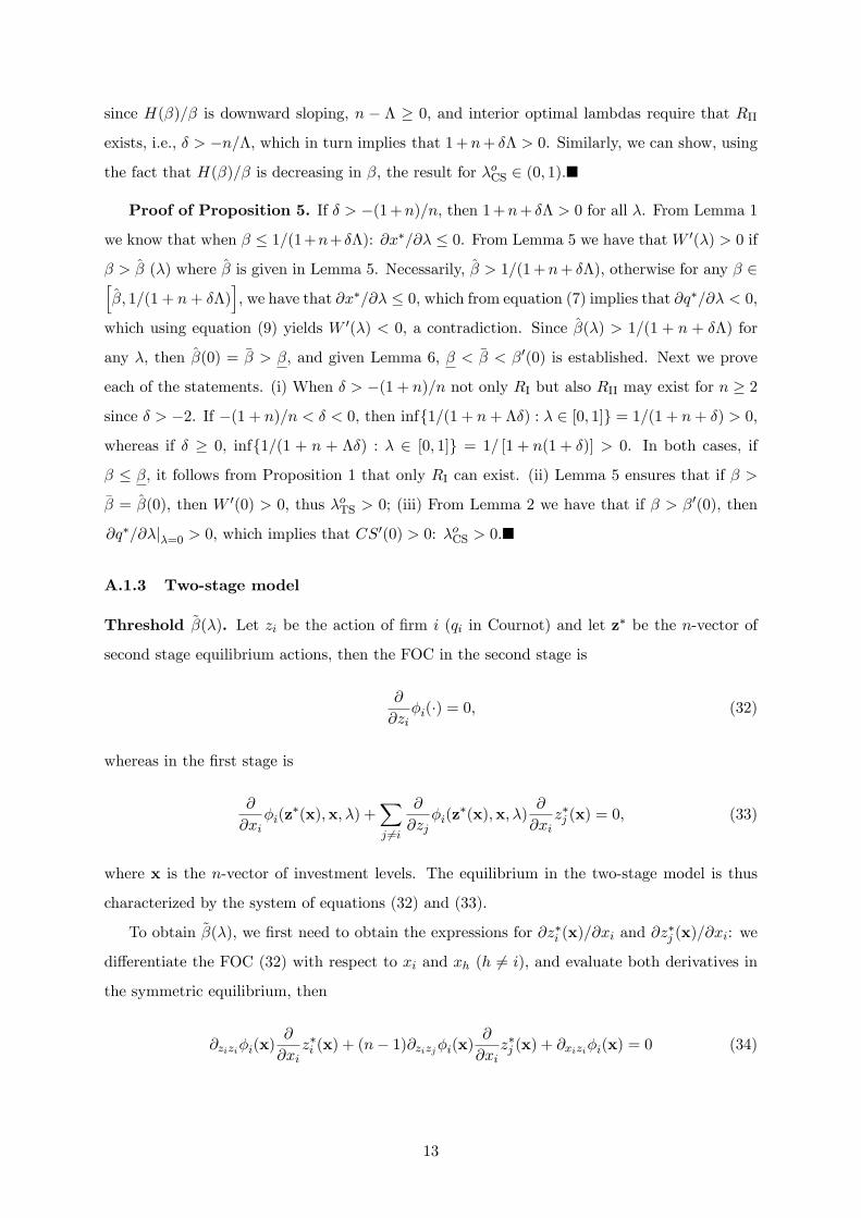
since H(�)=� is downward sloping, n � � � 0; and interior optimal lambdas require that RII

exists, i.e., � > �n=�, which in turn implies that 1+n+ �� > 0. Similarly, we can show, using

the fact that H(�)=� is decreasing in �, the result for �oCS 2 (0; 1).�

Proof of Proposition 5. If � > �(1+n)=n, then 1+n+ �� > 0 for all �. From Lemma 1

we know that when � � 1=(1+n+��): @x�=@� � 0. From Lemma 5 we have that W 0(�) > 0 if

� > �̂ (�) where �̂ is given in Lemma 5. Necessarily, �̂ > 1=(1+n+ ��), otherwise for any � 2h�̂; 1=(1 + n+ ��)

i, we have that @x�=@� � 0, which from equation (7) implies that @q�=@� < 0,

which using equation (9) yields W 0(�) < 0, a contradiction. Since �̂(�) > 1=(1 + n + ��) for

any �, then �̂(0) = �� > �, and given Lemma 6, � < �� < �0(0) is established. Next we prove

each of the statements. (i) When � > �(1 + n)=n not only RI but also RII may exist for n � 2

since � > �2. If �(1 + n)=n < � < 0, then inff1=(1 + n+ ��) : � 2 [0; 1]g = 1=(1 + n+ �) > 0,

whereas if � � 0, inff1=(1 + n + ��) : � 2 [0; 1]g = 1= [1 + n(1 + �)] > 0. In both cases, if

� � �, it follows from Proposition 1 that only RI can exist. (ii) Lemma 5 ensures that if � >

�� = �̂(0), then W 0(0) > 0, thus �oTS > 0; (iii) From Lemma 2 we have that if � > �0(0), then

@q�=@�j�=0 > 0, which implies that CS0(0) > 0: �oCS > 0.�

A.1.3 Two-stage model

Threshold ~�(�). Let zi be the action of �rm i (qi in Cournot) and let z� be the n-vector of

second stage equilibrium actions, then the FOC in the second stage is

@

@zi�i(�) = 0, (32)

whereas in the �rst stage is

@

@xi�i(z

�(x);x; �) +Xj 6=i

@

@zj�i(z

�(x);x; �)@

@xiz�j (x) = 0, (33)

where x is the n-vector of investment levels. The equilibrium in the two-stage model is thus

characterized by the system of equations (32) and (33).

To obtain ~�(�), we �rst need to obtain the expressions for @z�i (x)=@xi and @z�j (x)=@xi: we

di¤erentiate the FOC (32) with respect to xi and xh (h 6= i), and evaluate both derivatives in

the symmetric equilibrium, then

@zizi�i(x)@

@xiz�i (x) + (n� 1)@zizj�i(x)

@

@xiz�j (x) + @xizi�i(x) = 0 (34)

13

and

@zizj�i(x)@

@xiz�i (x) +

�@zizi�i(x) + (n� 2)@zizj�i(x)

� @

@xiz�j (x) + @xhzi�i(x) = 0. (35)

Solving (34) and (35) for @z�i (x)=@xi and @z�j (x)=@xi and rearranging terms, we obtain:

@

@xiz�i (x) =

1

�(�@xizi�i)

�@zizi�i � @zizj�i

�+ (n� 1) @zizj�i (@xhzi�i � @xizi�i)

�and

@

@xiz�j (x) =

1

�@xizi�i@zizj�i � @xhzi�i@zizi�i

�, (36)

where

��@zizi�i � @zizj�i

� �@zizi�i + (n� 1) @zizj�i

�. (37)

Consider Cournot competition, zi = qi. Then, we can rewrite (36) as follows:

@

@xiq�j (x) =

�c0(Bx)

@qiqi�i

�~�(�)� �

�, (38)

where

~�(�) =@qiqj�i@qiqi�i

=n(1 + �) + ��

2n+ ��

with 0 < ~�(�) � 1.

Proof of Lemma 3. We have that

~�(�) =n(1 + �) + ��

2n+ ��.

By di¤erentiating ~� with respect to n we obtain:

@~�

@n= � � (1� �)2

(2n+ ��)2.

Thus, for � < 1 and convex demand (� < 0), @~�=@n > 0; if demand is concave (� > 0),

@~�=@n < 0. Let us now di¤erentiate ~� with respect to �:

@~�

@�=

n2(� + 2)

(2n+ ��)2,

then, @~�=@� > 0 if � > �2. Finally, we di¤erentiate ~� with respect to �:

@~�

@�=�n (1� �)(2n+ ��)2

.

14

Thus, @~�=@� > 0 if � < 1.�

Proof of Lemma 4. Using (12), by totally di¤erentiating the system formed by (10; 11)

in a symmetric equilibrium, and solving for @q�=@� and @x�=@�, we obtain

@q�

@�=1~�f[@�xi�i + (n� 1) �] (@xiqi�i)B � @�qi�i [�x + x(n� 1)]g (39)

@x�

@�=1~�

�@�qi�i

�@xiqi�i� + (n� 1) q

�� [@�xi�i + (n� 1) �]�q

; (40)

where z � @ =@z with z = q; x; �, and

~�(Q�; x�) = �q [�x + x(n� 1)]� @xiqi�i�@xiqi�i� + q(n� 1)

�B;

which is assumed to be strictly positive.4 By rewriting equation (40) as follows

@x�

@�= #f 0(Q�)c0(Bx�)

�(� + s0(�)) [�(1 + �) + n]� [� + (n� 1)s(�)]

; (41)

where # � (n � 1)(Q�=n)= ~� and s(�) � !(�)(~�(�) � �), we get that sign f@x�=@�g is given

by (15). Let us now turn to the impact of � on output in equilibrium. Equation (39) can be

rewritten as follows

@q�

@�= #

�(� + s0(�))c0(Bx�)2B + f 0(Q�)

�c00(Bx�)(Q�=n)B [� + (n� 1)s(�)] + �00(x�)

�:

(42)

By inserting the FOC (11) evaluated in the symmetric equilibrium into the above expression,

after some manipulations we get that sign f@q�=@�g is given by (16). Finally, note that the

FOC with respect to output is identical to the one associated to the static case. Therefore, we

obtain again equation (7), which implies that if @x�=@� � 0, then @q�=@� < 0. From (15), we

obtain that @x�=@� > 0 if and only if

� > �2S � 1� (!0(�)~�(�) + !(�)~�0(�))P 0(c)�1n+ !(�)(n� 1)~�(�)(1 + n+ ��) + (n� 1)!(�)� P 0(c)�1n!0(�) :�

LEMMA 7 Under assumptions A.1.-A.4, in the two-stage model, there is a cut-o¤ spillover

value for spillovers (��2S < 1) above which allowing some overlapping ownership is socially

optimal (�oTS > 0) if

(1 + s0(0))n+ (1� s(0))(n� 1)((1 + s0(0))(1 + � + n)� [1 + (n� 1)s(0)]�H(1) > 0: (43)

4We show in Section A.2.2 that ~�(Q�; x�) > 0 is also a necessary condition for having a positive output atequilibrium in AJ.

15

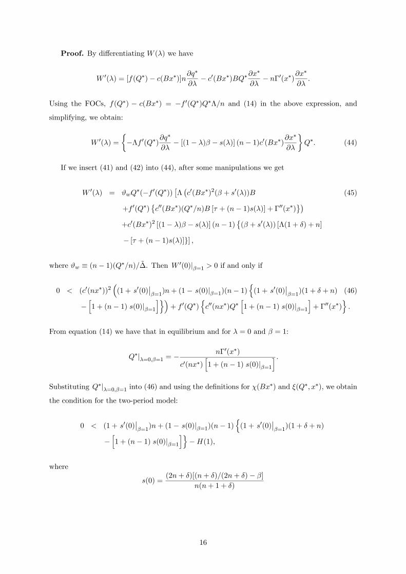
Proof. By di¤erentiating W (�) we have

W 0(�) = [f(Q�)� c(Bx�)]n@q�

@�� c0(Bx�)BQ�@x

�

@�� n�0(x�)@x

�

@�.

Using the FOCs, f(Q�) � c(Bx�) = �f 0(Q�)Q��=n and (14) in the above expression, and

simplifying, we obtain:

W 0(�) =

���f 0(Q�)@q

�

@�� [(1� �)� � s(�)] (n� 1)c0(Bx�)@x

�

@�

�Q�. (44)

If we insert (41) and (42) into (44), after some manipulations we get

W 0(�) = #wQ�(�f 0(Q�))

���c0(Bx�)2(� + s0(�))B (45)

+f 0(Q�)�c00(Bx�)(Q�=n)B [� + (n� 1)s(�)] + �00(x�)

�+c0(Bx�)2 [(1� �)� � s(�)] (n� 1)

�(� + s0(�)) [�(1 + �) + n]

� [� + (n� 1)s(�)]g] ,

where #w � (n� 1)(Q�=n)= ~�. Then W 0(0)j�=1 > 0 if and only if

0 < (c0(nx�))2�(1 + s0(0)

���=1

)n+ (1� s(0)j�=1)(n� 1)n(1 + s0(0)

���=1

)(1 + � + n) (46)

�h1 + (n� 1) s(0)j�=1

io�+ f 0(Q�)

nc00(nx�)Q�

h1 + (n� 1) s(0)j�=1

i+ �00(x�)

o.

From equation (14) we have that in equilibrium and for � = 0 and � = 1:

Q�j�=0;�=1 = �n�0(x�)

c0(nx�)h1 + (n� 1) s(0)j�=1

i .Substituting Q�j�=0;�=1 into (46) and using the de�nitions for �(Bx�) and �(Q�; x�), we obtain

the condition for the two-period model:

0 < (1 + s0(0)���=1

)n+ (1� s(0)j�=1)(n� 1)n(1 + s0(0)

���=1

)(1 + � + n)

�h1 + (n� 1) s(0)j�=1

io�H(1),

where

s(0) =(2n+ �)[(n+ �)=(2n+ �)� �]

n(n+ 1 + �)

16

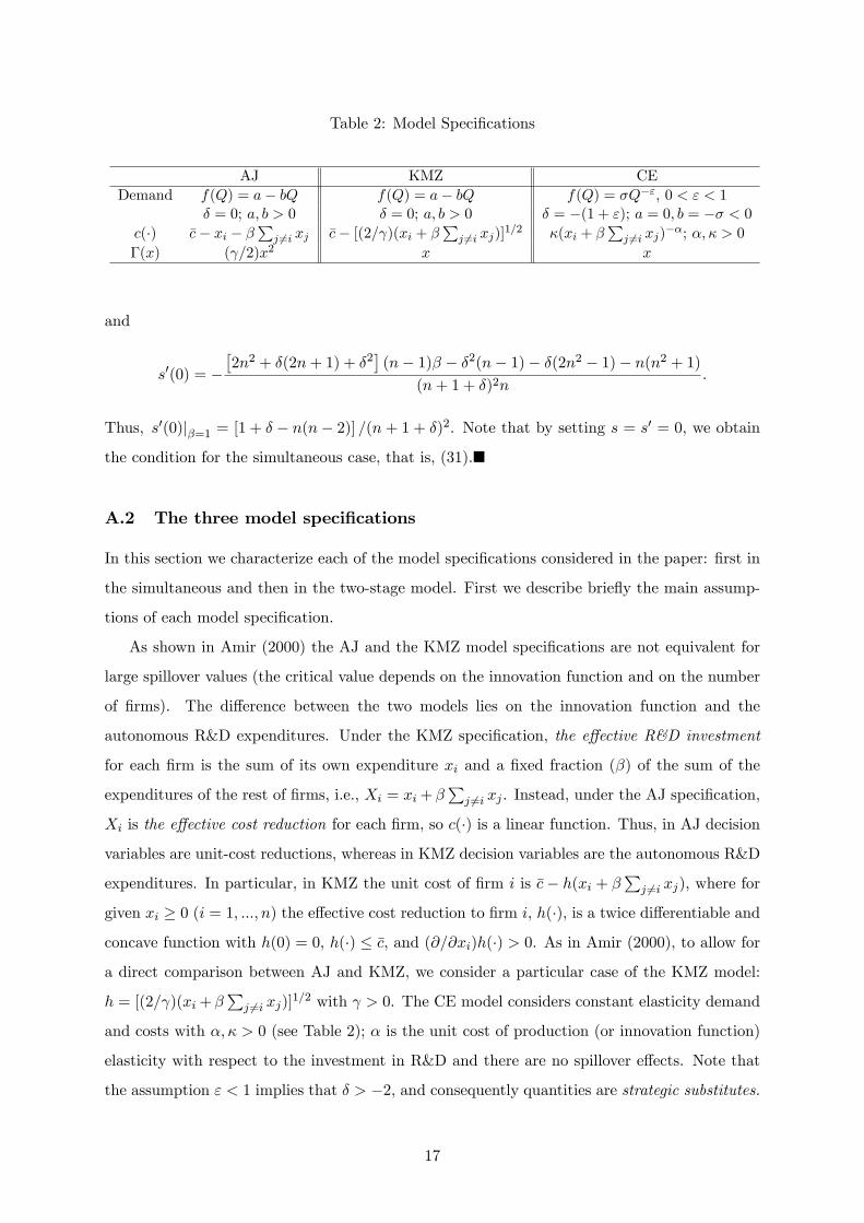
Table 2: Model Speci�cations

AJ KMZ CEDemand f(Q) = a� bQ f(Q) = a� bQ f(Q) = �Q�"; 0 < " < 1

� = 0; a; b > 0 � = 0; a; b > 0 � = �(1 + "); a = 0; b = �� < 0c(�) �c� xi � �

Pj 6=i xj �c� [(2= )(xi + �

Pj 6=i xj)]

1=2 �(xi + �Pj 6=i xj)

��; �; � > 0�(x) ( =2)x2 x x

and

s0(0) = ��2n2 + �(2n+ 1) + �2

�(n� 1)� � �2(n� 1)� �(2n2 � 1)� n(n2 + 1)

(n+ 1 + �)2n.

Thus, s0(0)j�=1 = [1 + � � n(n� 2)] =(n + 1 + �)2. Note that by setting s = s0 = 0, we obtain

the condition for the simultaneous case, that is, (31).�

A.2 The three model speci�cations

In this section we characterize each of the model speci�cations considered in the paper: �rst in

the simultaneous and then in the two-stage model. First we describe brie�y the main assump-

tions of each model speci�cation.

As shown in Amir (2000) the AJ and the KMZ model speci�cations are not equivalent for

large spillover values (the critical value depends on the innovation function and on the number

of �rms). The di¤erence between the two models lies on the innovation function and the

autonomous R&D expenditures. Under the KMZ speci�cation, the e¤ective R&D investment

for each �rm is the sum of its own expenditure xi and a �xed fraction (�) of the sum of the

expenditures of the rest of �rms, i.e., Xi = xi+ �Pj 6=i xj . Instead, under the AJ speci�cation,

Xi is the e¤ective cost reduction for each �rm, so c(�) is a linear function. Thus, in AJ decision

variables are unit-cost reductions, whereas in KMZ decision variables are the autonomous R&D

expenditures. In particular, in KMZ the unit cost of �rm i is �c� h(xi + �Pj 6=i xj), where for

given xi � 0 (i = 1; :::; n) the e¤ective cost reduction to �rm i, h(�), is a twice di¤erentiable and

concave function with h(0) = 0, h(�) � �c, and (@=@xi)h(�) > 0. As in Amir (2000), to allow for

a direct comparison between AJ and KMZ, we consider a particular case of the KMZ model:

h = [(2= )(xi+ �Pj 6=i xj)]

1=2 with > 0. The CE model considers constant elasticity demand

and costs with �; � > 0 (see Table 2); � is the unit cost of production (or innovation function)

elasticity with respect to the investment in R&D and there are no spillover e¤ects. Note that

the assumption " < 1 implies that � > �2, and consequently quantities are strategic substitutes.

17

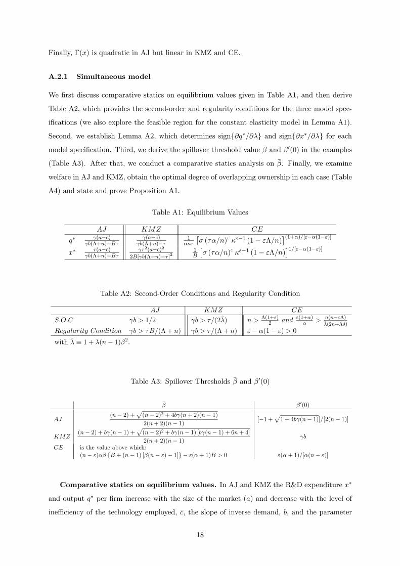
Finally, �(x) is quadratic in AJ but linear in KMZ and CE.

A.2.1 Simultaneous model

We �rst discuss comparative statics on equilibrium values given in Table A1, and then derive

Table A2, which provides the second-order and regularity conditions for the three model spec-

i�cations (we also explore the feasible region for the constant elasticity model in Lemma A1).

Second, we establish Lemma A2, which determines signf@q�=@�g and signf@x�=@�g for each

model speci�cation. Third, we derive the spillover threshold value �� and �0(0) in the examples

(Table A3). After that, we conduct a comparative statics analysis on ��. Finally, we examine

welfare in AJ and KMZ, obtain the optimal degree of overlapping ownership in each case (Table

A4) and state and prove Proposition A1.

Table A1: Equilibrium Values

AJ KMZ CE

q� (a��c) b(�+n)�B�

(a��c) b(�+n)��

1���

�� (��=n)" �"�1 (1� "�=n)

�(1+�)=["��(1�")]x� �(a��c)

b(�+n)�B� �2(a��c)2

2B[ b(�+n)�� ]21B

�� (��=n)" �"�1 (1� "�=n)

�1=["��(1�")]

Table A2: Second-Order Conditions and Regularity Condition

AJ KMZ CE

S:O:C b > 1=2 b > �=(2~�) n > �(1+")2 and "(1+�)

� > n(n�"�)~�(2n+��)

Regularity Condition b > �B=(� + n) b > �=(� + n) "� �(1� ") > 0with ~� � 1 + �(n� 1)�2.

Table A3: Spillover Thresholds �� and �0(0)

�� �0(0)

AJ(n� 2) +

p(n� 2)2 + 4b (n+ 2)(n� 1)2(n+ 2)(n� 1) [�1 +

p1 + 4b (n� 1)]=[2(n� 1)]

KMZ(n� 2) + b (n� 1) +

p(n� 2)2 + b (n� 1) [b (n� 1) + 6n+ 4]2(n+ 2)(n� 1) b

CE is the value above which:(n� ")�� fB + (n� 1) [�(n� ")� 1]g � "(�+ 1)B > 0 "(�+ 1)=[�(n� ")]

Comparative statics on equilibrium values. In AJ and KMZ the R&D expenditure x�

and output q� per �rm increase with the size of the market (a) and decrease with the level of

ine¢ ciency of the technology employed, �c, the slope of inverse demand, b, and the parameter

18

(which is the parameter of the slope of the R&D costs in AJ). In the CE model x� and q�

increase with the size of the market, �. In addition, the costlier the technology employed, �,

the lower is total output, Q�. However, x� decreases (respectively, increases) with � if demand

is elastic (inelastic). The last two results hold for any value of � and �.5

Derivation of Table A2. In AJ and KMZ it is immediate that @qiqi�i = �2b < 0.

Furthermore, in AJ: condition @qiqi�i (@xixi�i)� (@qixi�i)2 > 0, given by (21), can be written as

2b � 1 > 0, since c00(�) = 0 and �00(x) = , so @xixi�i = � and @qixi�i = �c0(�) = 1. In KMZ,

(21) can be written as

"1

2

�2

(Bx�)

��1#� 2b

"1

2

�2

(Bx�)

��3=2#q�~� < 0. (47)

From FOC (3) we have that in equilibrium

q� =�0(x�)

�c0(Bx�)� =1

(1= ) [(2(Bx�)= ]�1=2 �. (48)

Inserting the above equation into condition (47), after some manipulations, it reduces to 1 �

2b ~�=� < 0. (Note that if b > �=2 holds, then the condition b > �=(2~�) is satis�ed.) In AJ

and from (20), it is immediate that � = b(� + n) � �B since c00(�) = � = 0; f 0(Q) = �b and

�0(x) = x. In KMZ we have:

� = �"1

2

�2

Bx�

��3=2B�

1

(1= )(2Bx�= )�1=2�

#[�b (� + n)]� 1

2

�2

Bx�

��1�B

=1

�2

Bx�

��1 �Bb(� + n)� �B

�.

Therefore, in KMZ � > 0 if b > �=(� + n). Regarding the constant elasticity model we have:

LEMMA A1 (Constant elasticity model) At the equilibrium, for a given n � 2 and � � 0,

second order conditions together with the condition of non-negative pro�ts require that

(i) maxf"�;�(1 + ")=2g < n � "�(B + ��)=(��),

(ii) "(1 + �)=� > n(n� "�)=h~�(2n+ ��)

i, with ~� � 1 + �(n� 1)�2.

Furthermore, the equilibrium is regular if and only if (1 + �)=� > 1=".

Proof. From the FOC (2) we need that

n > "�, (49)

5The same result is obtained in Dasgupta and Stiglitz (1980) for � = � = 0 and free entry.

19

otherwise the system (2; 3) will not have a solution. Since � = �(1+"), �q < 0 if condition (49)

holds (see Table 4). This condition also guarantees that Q� and x� are both positive. Notice

that @qiqi�i < 0 if (f0(Q�)=n)(2n+ ��) < 0, then @qiqi�i < 0 if

n > �(1 + ")=2. (50)

Since � 2 [1; n], we have that the latter condition is always satis�ed for " < 1. By construction

@xixi�i < 0. Furthermore, second order condition @qiqi�i (@xixi�i) � (@qixi�i)2 > 0, which is

given by (21), reduces to

�"�nQ��("+1)(2n+ ��)

h�(�+ 1)�(Bx�)�(�+2)(Q�=n)~�

i+ (��)2(Bx�)�2(�+1) < 0. (51)

From the FOC (2) we have that at the symmetric equilibrium

Q� = [�(n� "�)=(n�)]1=" (Bx�)�=". (52)

By substituting (52) into (51), after some manipulations, we obtain

(Bx�)�2(�+1)��2n� ["=(n� "�)] (2n+ ��)(�+ 1)~�=n+ �

o< 0.

The above condition is satis�ed if "(�+1)=� > n(n�"�)=[(2n+��)~�], which proves statement

(ii) of the Proposition.

From (20) we have that � > 0 if

0 < ��(�+ 1)�(Bx�)�(�+2)(Q�=n)�Bh"(1 + ")�Q��("+2)�Q� � "�Q��("+1)(� + n)

i�(��)2(Bx�)�2(�+1)�B, or

0 < Q��("+1)h��(�+ 1)�(Bx�)�(�+2)(Q�=n)�B

i["(1 + ")��� "�(� + n)]

�(��)2(Bx�)�2(�+1)�B.

Substituting (52) into the above expression, we obtain

0 < ���(n� "�)

n�

��("+1)="(Bx�)�("+1)�="�(�+ 1)�(Bx�)�(�+2)

��(n� "�)

n�

�1="(Bx�)�="

�B

n["(1 + ")��� "�(� + n)]� (��)2(Bx�)�2(�+1)�B,

20

rearranging terms yields

0 < (Bx�)�2(�+1)�

n�

�(n� "�)

���(�+ 1)��B

n

���"�n+ "2��

�� (��)2�B

�, or equivalently,

0 < (Bx�)�2(�+1)��2�B ["(�+ 1)� �] .

Therefore, � > 0 holds if (1 + �)=� > 1=", or, equivalently, if "� �(1� ") > 0.

We turn now to deriving the condition under which pro�ts in equilibrium are nonnegative. At

the symmetric equilibrium, each �rm�s pro�t is given by �(Q�=n; x�) = [f(Q�)� c(Bx�)] (Q�=n)�

x�. Then, �(Q�=n; x�) � 0 if �� � [f(Q�)� c(Bx�)]Q�=(x�n) � 1. Write

#CE � ����n

�"�"�1

�n� "�n

�.

Then Q� = [n=(���)] #CE (1+�)=["��(1�")], x� = (1=B) #CE 1=["��(1�")], and condition �� � 1 can

be expressed as

��� n

���

��"#CE

�"(1+�)=["��(1�")] � � #CE ��=["��(1�")]�1

���#CE

�=["��(1�")]B � 1.

Rearranging terms, and replacing #CE into the above expression, we get ["�=(n� "�)] [B=(��)] �

1. It follows that �� � 1 if �"�

��

�(B + ��) � n. (53)

Combining conditions (49), (50) and (53) yields statement (i).�

21

Fig. A1. Feasible region for the CE

model with n = 7.

Feasible region for the constant elasticity model with � = 0. From Lemma A1

we have that � > 0 if (1 + �)=� > 1=". When � = 0, the LHS of condition (i) is satis�ed

for any n � 2 since " < 1, moreover the RHS of condition (i) can be rewritten as follows

n � �CE(�) = "(1 + � � �)=(� � "�). Since �0CE > 0 (as we are also imposing that � > 0),

condition n � �CE(�) will hold for all � if n � "(1 + �)=�. Last, condition (ii) with � = 0

writes as "(1 + �)=� > n(n � ")= [2n� (1 + ")]. Therefore, at � = 0 we only have to consider

the RHS of condition (i) and condition (ii). These two conditions are depicted in Fig. A1 for

n = 7; the grey area are combinations (�; ") for which the two conditions are satis�ed (these

combinations of parameters also satisfy the two conditions for n � 7).

Determination of signf@q�=@�g and signf@x�=@�g in AJ, KMZ and CE. Note that

@q�=@� can be written in the following manner

@q�

@�=(n� 1)(Q�=n)

�

n�c0(Bx�)

�2�B + f 0(Q�)

�c00(Bx�)(Q�=n)B� + �00(x�)

�o, (54)

then after some calculations, it is simple to verify that in the simultaneous model:

LEMMA A2 We have (i) In AJ: sign�@q�

@�

�= signf�(1+�(n� 1))� b g and sign

�@x�

@�

�=

signf�(n + 1) � 1g; (ii) In KMZ: sign�@q�

@�

�= signf� � bg and sign

�@x�

@�

�= signf�(n +

1)�1g; (iii) In the CE model: sign�@q�

@�

�= signf� [�(n� "�)� �(n� 1)"(�+ 1)]�"(�+1)g

22

and sign�@x�

@�

�= signf� [(n� ")� �(n� 1)(1 + ")]� 1g.

Derivation of �� (Table A3). Note that @x�=@� can be written as

@x�

@�=(n� 1)(Q�=n)f 0(Q�)c0(Bx�)

�[�(�(1 + �) + n)� � ] (55)

If we insert equations (54) and (55) into equation (9), after some manipulations we obtain

W 0(�) =�(n� 1)(Q�)2=(n�)

�(�f 0(Q�))z, where

z � �f�c0(Bx�)

�2�B + f 0(Q�)[c00(Bx�)(Q�=n)B� + �00(x�)]g

+�c0(Bx�)

�2(1� �)�(n� 1) f� [�(1 + �) + n]� �g .

By noting that in AJ: f 0 = �b, � = 0, c0 = �1, c00 = 0 and �00 = , it then follows that

zAJ = zj�=0 = �B � b + �(n� 1) [�(1 + n)� 1]

= (n� 1)(n+ 2)�2 � (n� 2)� � b .

By solving zAJ = 0 for � we obtain the expression for ��AJ . Notice that ��AJ < 1 if

(n� 2) +p(n� 2)2 + 4b (n+ 2)(n� 1) < 2(n+ 2)(n� 1),

or

(n� 2)2 + 4b (n+ 2)(n� 1) < [2(n+ 2)(n� 1)� (n� 2)]2 ,

which can be rewritten as 4b (n+2)(n� 1) < 4n2(n+2)(n� 1). Thus, ��AJ < 1 if b < n2. In

KMZ we have c = �c�q(2= )(xi + �

Pj 6=i xj), f

0 = �b, � = 0 and �00 = 0, then

zKMZ = zj�=0 =�

2 x�+

�bq�B 2 (2Bx�= )3=2

+�(n� 1) [�(1 + n)� 1]

2 Bx�

=1

B

�bq�B1=2

2 (2x�= )3=2+

�

2 x�fB + (n� 1) [�(1 + n)� 1]g

!.

By replacing q� and x� into the above expression, after some calculations we get

zKMZ =[b (1 + n)� 1]2

(a� �c)2

��bB + �

fB + (n� 1) [�(1 + n)� 1]g

�.

23

It is then immediate that: zKMZ > 0 , � > ��KMZ . Notice that ��KMZ

< 1 if

�(n� 2)2 + b (n� 1) [b (n� 1) + 2(3n+ 2)]

1=2< 2(n+ 2)(n� 1)� n+ 2� b (n� 1),

which can be rewritten as 4n(n + 2)(n � 1)(�n + b ) < 0. In the constant elasticity model

f = �Q�", c = �(xi + �Pj 6=i xj)

�� and �(x) = x, then

zCE = zj�=0 = (��)2(Bx�)�2(�+1)�B � "�(Q�)�"�1�(�+ 1)�(Bx�)�(�+2)q�B

+(��)2(Bx�)�2(�+1)�(n� 1) [�(�"+ n)� 1] .

By replacing q� and x� into the above expression, we obtain

zCE = �2�2z�2(1+�)�B � "� [n=(��)]�(1+") z�(1+�)(1+")(�+ 1)z�(�+2)z�+1B (56)

+�2�2z�2(1+�)�(n� 1) [�(�"+ n)� 1] ,

where

z �h����n

�"�"�1 (1� "=n)

i1=["��(1�")].

By noting that z�(�+1)(1+")�(�+2)+(�+1) = z�"+�(1�")z�2(1+�) we can re-write equation (56) as

follows

zCE = z�2(1+�)��2 f��B + ��(n� 1) [�(�"+ n)� 1]� "(�+ 1)B=(n� ")g .

Hence zCE > 0 if and only if

(n� ")�� fB + (n� 1) [�(n� ")� 1]g � "(�+ 1)B > 0.�

24

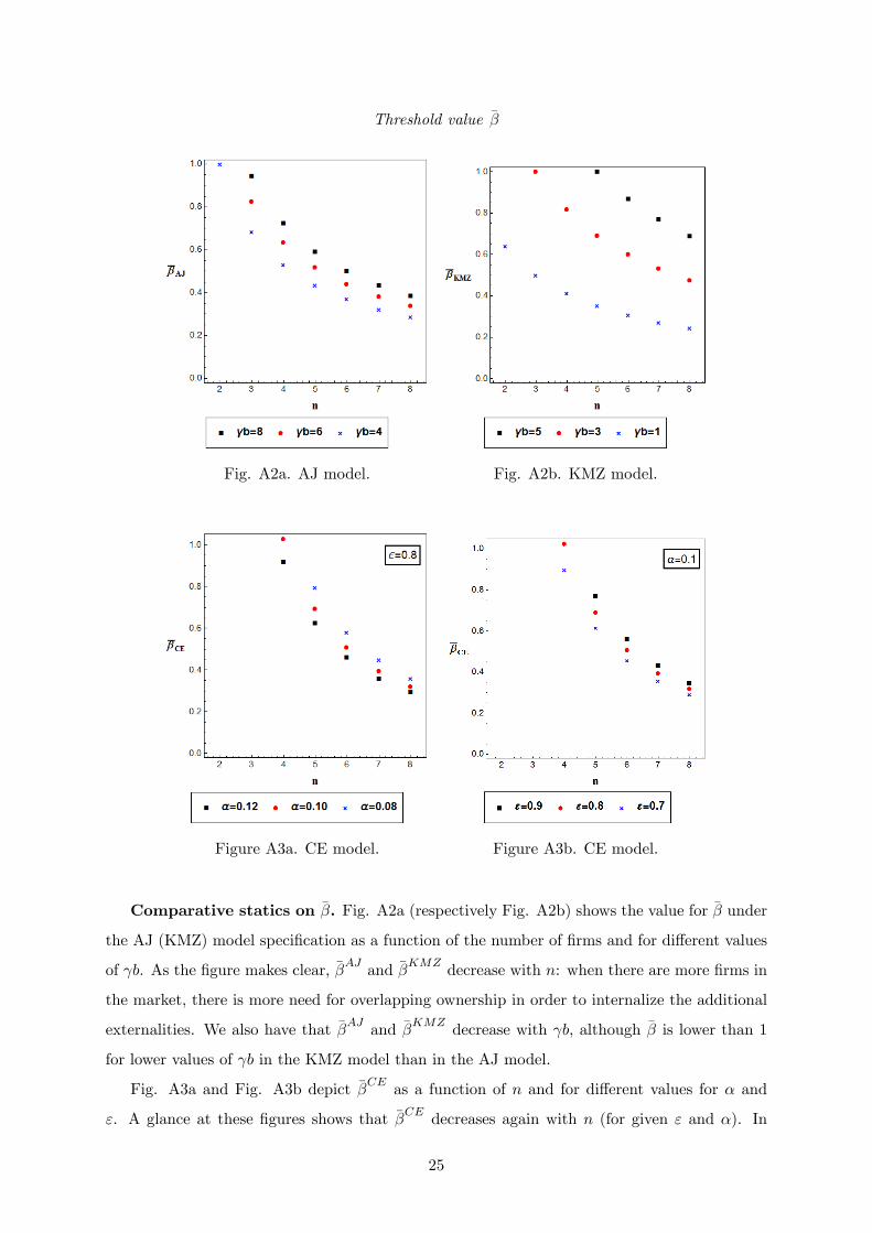
Threshold value ��

Fig. A2a. AJ model. Fig. A2b. KMZ model.

Figure A3a. CE model. Figure A3b. CE model.

Comparative statics on ��. Fig. A2a (respectively Fig. A2b) shows the value for �� under

the AJ (KMZ) model speci�cation as a function of the number of �rms and for di¤erent values

of b. As the �gure makes clear, ��AJ and ��KMZ decrease with n: when there are more �rms in

the market, there is more need for overlapping ownership in order to internalize the additional

externalities. We also have that ��AJ and ��KMZ decrease with b, although �� is lower than 1

for lower values of b in the KMZ model than in the AJ model.

Fig. A3a and Fig. A3b depict ��CE as a function of n and for di¤erent values for � and

". A glance at these �gures shows that ��CE decreases again with n (for given " and �). In

25

Table A4: Optimal Degree of Cross-ownership in AJ and KMZ

�oTS

AJ minnmax

n0; [(n+2)(n�1)��(n�2)]��b (n�1)[2(��1)�+b ]

o; 1o

KMZ minnmax

n0; [(n+2)(n�1)��b (n�1)�(n�2)]��b (n�1)f[2�+b (n�1)�2]�+b g

o; 1o

addition, Fig. A3a tells us that for given n and ", ��CE decreases with the elasticity of the

innovation function, �, whereas Fig. A3b shows that for given n and �, ��CE increases with ",

so it decreases with the elasticity of demand. We also have that for the (feasible) combination

of parameters (�; ") considered here, ��CE � 1 when there are two or three �rms in the market.

Optimal degree of overlapping ownership (TS and CS standard)

Fig. A4a. CE model.

(� = 0:1, � = � = 1, n = 8, � = 0:8)

Fig. A4b. CE model.

(" = 0:8, � = � = 1, n = 8, � = 0:8)

Fig. A4a and A4b show that the greater is the elasticity of demand, "�1, or the elasticity

of the innovation function, �, the greater should be the degree of overlapping ownership if the

social planner seeks to maximize total surplus; however, if the objective is to maximize consumer

surplus, then for the same parameter range, �oCS = 0.

Welfare in AJ and KMZ. Here, we show that welfare is a single-peaked function in AJ

and KMZ; we also derive �oTS under these two model speci�cations (Table A4).

26

Case AJ: By inserting equilibrium values into the welfare function we get

W =1

2n (a� �c)2 (2� + n) b� �

2

[(� + n) b�B� ]2.

If we di¤erentiate W with respect to � we obtain:

dW

d�= �(n� 1)(a� �c) b f� b+ � [2� (B � n) + n� 2� �(n+ 2)(n� 1)]g

[(� + n) b �B� ]2Q.

Note that solving dW=d� = 0 for � yields a unique stationary point, given by �̂AJ . By taking

the second order derivative with respect to �, evaluating it at � = �̂AJ , and simplifying, we

obtaind2W

d�2

�����=�̂AJ

= � (n� 1)2(a� �c) b [2 (� � 1)� + b]3��(n+ 2)(n� 1)2�4 � 6(n� 1)�3 + Z1 + 2Z2 � Z3

�2Q,where Z1 �

��n2 + 4n� 1

� b+ 3 (n� 2)

��2, Z2 � 2 [ b(1� 2n) + 1]� and Z3 � b(1 � bn).

The second order condition requires that b > 1=2 (see Table A2), then 2(� � 1)� + b > 0 for

any � 2 [0; 1], and as a result: d2W=d�2���=�̂AJ

< 0. Since �̂AJ is the unique stationary point

of W , it follows that �̂AJ is a global maximum. This is the desired �oTS.

Case KMZ: By inserting equilibrium values into the welfare function we get

W =1

2n (a� �c)2 (2� + n)B b� �

2

[(� + n) b� � ]2B.

By di¤erentiating W with respect to � we obtain:

dW

d�= �(n� 1)(a� �c) b f�B b+ � [2� (B � n) + n� 2� �(n+ 2)(n� 1)]g

B [(� + n) b � � ]2Q,

and by solving dW=d� = 0 for � we get a unique stationary point, given by �̂KMZ . The second

order derivative with respect to � evaluated at � = �̂KMZ yields

d2W

d�2

�����=�̂KMZ

= b(n� 1)2(a� �c)B [(� + n) b� � ]3

ZKMZQ,

where ZKMZ � � [�n+ (1� �)]n( b)2+�4�(1� �)n+ (1� �)2 � �2n2

� b+�B [�(n+ 2)� 2].

The regulatory condition requires that b > �=(�+n) (see Table A2), thus d2W=d�2���=�̂KMZ

<

0 whenever ZKMZ < 0. Since �̂KMZ is the unique stationary point of W , it follows that �̂KMZ

is a global maximum whenever ZKMZ < 0. This is the desired �oTS. It is straightforward to show

that the regularity condition is stricter than the second order condition under the KMZ model

speci�cation for n > 2 (see Table A2). In addition, the regularity condition becomes stricter

27

as � and n increase. For � = 1, the maximum value of the right-hand side of the regularity

condition ispn(n�1)= [4(n�

pn)], which for example equals 0:60 for n = 2 and 0:68 for n = 3.

Numerical simulations show that assuming b > 0:62 guarantees that ZKMZ < 0 holds for any

n; thus, ZKMZ < 0 is a mild condition: it is slightly stricter than the regularity condition in

duopoly but softer for oligopoly of three or more �rms.�

PROPOSITION A1 A Research Joint Venture with no overlapping ownership (� = 0 and

� = 1) is socially optimal in AJ when b � n2, in KMZ when b � n, and in CE (provided

that W (�) is single peaked) when � � "n=[(n� 1)"2 + (�1 + n� 2n2)"+ n(n2 + 1� n)].

Proof. When W (�) is single peaked, �� is the minimum threshold above which allowing

some positive � is welfare enhancing (Proposition 4). Consequently, �oTS = 0 for any � 2 [0; 1]

if �� � 1. From Table A3 we have that ��AJ � 1 if b � n2 and ��KMZ � 1 if b � n;

in both cases W (�) is single peaked (see above). Also, from Table A3 we obtain ��CE , and

solving ��CE = 1 for �, yields the threshold value in terms of n and ": ��CE � 1 if � �

"n=[(n � 1)"2 + (�1 + n � 2n2)" + n(n2 + 1 � n)]. Next we show that for � = 0, W 0(�) > 0

under AJ, KMZ and CE model speci�cations, and therefore it is socially optimal to set � = 1

in the three cases. We can write

@W

@�= (f(Q�)n� nc(Bx�)) @q

�

@�� nc0(Bx�)(n� 1)x�q� � nc0(Bx�)B@x

�

@�q� (57)

�n�0(x�)@x�

@�

=

���f 0(Q�)@q

�

@�� (1� �)�(n� 1)c0(Bx�)@x

�

@�� c0(Bx�)(n� 1)x�

�Q�.

In AJ and for � = 0, @q�=@� > 0 and @x�=@� > 0 (see Table A1), thus from (57) it is clear

that @W=@� > 0. In KMZ and for � = 0, @q�=@� = 0 and @x�=@� < 0. Higher R&D spillovers

reduce R&D expenditures but also the unit cost of production of all �rms. The latter dominates

the former:@W

@�

�����=0

=1

2

n(a� �c)2 (n� 1)[b (n+ 1)� 1]2B2

> 0.

In CE and for � = 0, @q�=@� = 0 and @x�=@� < 0. As in KMZ, welfare is increasing in �:

@W

@�

�����=0

=n����n

�"�"�1

�1� "

n

�� 1"��(1�") (n� 1)

B2> 0.�

28

Snapshot of the Application

Fig. A5. AJ model. (a = 700, �c = 500, = 8:5, � = 0:5, b = 0:6)

29

Optimal degree of overlapping ownership (TS and CS standard)

Fig. A6a. KMZ model.

( = 3, n = 6, b = 0:3)

Fig. A6b. KMZ model.

( = 3, � = 0:8, b = 0:3)

Table A5: E¤ect of Parameters on �oTS and �oCS

�oTS �oCSAJ KMZ CE AJ KMZ CE

Number of �rms (n) + + + h+i 0 (+)Elasticity of demand (b�1; "�1) + + + h+i h+i [+]Elasticity of innovation function ( �1; �) + + h+i h+i [+]Degree of spillover (�) + + + (+) (+)� [+]

Key: h+i, the parameter enlarges the region where �oCS = 1; (+), the e¤ect is positive only if both � and n

are su¢ ciently large (otherwise there is no e¤ect); (+)�, the e¤ect is positive only if the parameter is su¢ ciently

large and b is su¢ ciently small (otherwise there is no e¤ect); [+], the e¤ect is positive when n is su¢ ciently

large (otherwise there is no e¤ect).

A.2.2 Two-stage model

Next we present equilibrium values of output and R&D together with the expressions for

signf@q�=@�g and signf@x�=@�g for each model speci�cation. After that, we conduct a com-

parative statics analysis on ��, and on �oTS and �oCS. Finally, we compare the static and the

two-stage model and brie�y discuss the comparative statics on the other parameters of the

model.

Equilibrium values and sign f@q�=@�g and sign f@x�=@�g. We consider each case in

turn.

30

Case AJ: FOCs (10; 14) yield

�b�q� + a� bnq� � �c+Bx� = 0

�� +

�

n+ �(n� 1) (1 + �� 2�)

�q� � x� = 0.

Solving the system for equilibrium values gives

q� = (a� �c)

~�and x� =

h(n� 1)( �

n+�)(1 + �� 2�) + �i(a� �c)

~�

where

~� � b(� + n)2 �B [(n� 1)�(1 + �� 2�) + (n+ �)� ]� + n

.

In this case, as in the simultaneous model, H(�) = b , then using (16) we obtain

sign

�@q�

@�

�= sign

�(B� � b ) (n+ �) +B

�1 + �� 2�n+ �

(n� 1)n+ ���

and using (15) we get

sign

�@x�

@�

�= signf� [� + n+ (n� 1)(!(�)� �)] (58)

+

�1 + �� 2�n+ �

(n� 1)n+ ��� 1� (n� 1)!(�)~�(�)g,

where we have used that

h!0(�)(~�(�)� �) + !(�)~�0(�)

i(� + n) =

1 + �� 2�n+ �

(n� 1)n+ �.

Case KMZ: The output and R&D values in equilibrium are given by (10; 14):

�b�q� + a� bnq� � �c+��2

�Bx�

�1=2= 0

1

��2

�Bx�

��1=2 �� + (n� 1) �

n+ �(1 + �� 2�)

�q� � 1 = 0.

Solving the system for equilibrium values gives

q� = (a� �c)

b(� + n)� � and x� =

1

2

(a� �c)2#2KMZ

B [b (� + n)� �]2

with #KMZ � � + s(�)(n� 1) = (n� 1) �n+� (1 + �� 2�) + � , where s(�) � !(�)(~�(�)� �).

31

In this case, as in the simultaneous model, H(�) = b B, then from (16) we have

sign

�@q�

@�

�= sign

�(� � b )(n+ �) +

�1 + �� 2�n+ �

(n� 1)n+ ���

and signf@x�@� g is again given by (58).

Case CE: The output and R&D values in equilibrium are obtained from (10; 14):

�Q��"�1� "�

n

�� �(Bx�)�� = 0

�(Bx�)���1h� + (n� 1)!(�)(~�(�)� �)

i Q�n= 1.

Solving the system for Q� and x�, after some manipulations, we get

Q� =n

�� [(n� 1)s(�) + � ]

��

�[(n� 1)s(�) + � ]�

n

�"�"�1

�1� "�

n

��(1+�)=["��(1�")]and

x� =1

B

��

�[(n� 1)s(�) + � ]�

n

�"�"�1

�1� "�

n

��1=["��(1�")],

where s(�) � !(�)(~�(�)� �) with

!(�) =� [2n� �(1 + ")]

n(n� "�) and ~�(�) =n(1 + �)� �(1 + ")2n� �(1 + ") .

Hence, we have

sign

�@q�

@�

�= sign

��� + s0(�)

�� �+ 1

�

"

n� "� [(n� 1)s(�) + � ]�.

And, one can obtain signf@x�=@�g by inserting values into (15) with � = �(1 + ").

32

Threshold value ��

Fig. A7a. AJ model. Fig. A7b. KMZ model.

Fig. A8a. CE model. Fig. A8b. CE model.

Comparative statics on ��. Fig. A7a and A7b depict, respectively, the threshold ��2S

under the AJ and KMZ model speci�cations. Fig. A7b reveals that in KMZ, ��2S tends to be

above 1 if we consider the same values as in AJ. In particular, only if b is low enough, we have

that ��2S < 1 (this result is in line with the simultaneous model). Also, we observe that under

the AJ and KMZ model speci�cations, ��2S decreases with the number of �rms and increases

with b. Figures A8a (respectively A8b) depict the threshold ��2S for the CE model for a given

" (�) and di¤erent values of n and � ("). As in the simultaneous model, the threshold value

decreases with n, the elasticity of the innovation function, �, and the elasticity of demand "�1.

33

Comparative statics on �oTS and �oCS. Fig. A9 is a snapshot of the application and

plots welfare, consumer surplus, pro�t, price, cost, q� and x� as functions of � (for � = 0:65 and

n = 6). Fig. A10a, A10b and A10c show, respectively, optimal lambdas in AJ, KMZ and CE as

functions of the number of �rms. We see that under the three model speci�cations, �oTS weakly

increases with n, whereas �oCS jumps with n only in AJ (and only for n su¢ ciently large).

Snapshot of the Application

Fig. A9. AJ model. (a = 700, �c = 500, = 7, n = 6, b = 0:6)

34

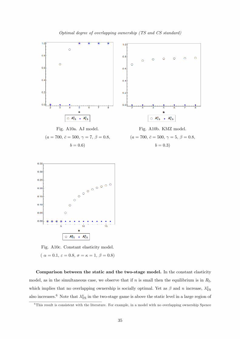
Optimal degree of overlapping ownership (TS and CS standard)

Fig. A10a. AJ model.

(a = 700, �c = 500, = 7, � = 0:8,

b = 0:6)

Fig. A10b. KMZ model.

(a = 700, �c = 500, = 5, � = 0:8,

b = 0:3)

Fig. A10c. Constant elasticity model.

( � = 0:1, " = 0:8, � = � = 1, � = 0:8)

Comparison between the static and the two-stage model. In the constant elasticity

model, as in the simultaneous case, we observe that if n is small then the equilibrium is in RI,

which implies that no overlapping ownership is socially optimal. Yet as � and n increase, �oTS

also increases.6 Note that �oTS in the two-stage game is above the static level in a large region of

6This result is consistent with the literature. For example, in a model with no overlapping ownership Spence

35

spillovers. For low values of �, the strategic e¤ect is positive. Then, the two-stage model behaves

di¤erently than the static model in that welfare can increase with � in RI because it reduces

R&D overinvestment by �rms. This case is illustrated in Figure A11, where� for low �� �oTS

in the two-stage model is larger than in the static model. For intermediate values of spillovers,

the strategic e¤ect becomes negative (but remains close to zero); for higher spillover values, �oTS

increases with � more rapidly (i.e., convexly) when the strategic e¤ect is strong.

Fig. A11. Constant elasticity model.

(� = 0:1, " = 0:8, � = � = 1, n = 8.)

Fig A12. AJ model.

( = 7, n = 6, b = 0:6.)

In the AJ model, we �nd that �oTS and �oCS are weakly larger in the two-stage case (see

Figure A12). In contrast with the static model, the simulations indicate (for � = 0:65 and

n = 6) that prices may be hump-shaped while cost decreases with �; correspondingly, output

per �rm is U-shaped when R&D per �rm increases. The welfare translation of the increase

in � displays U-shaped consumer surplus and increasing pro�t per �rm, which results in an

interior solution for welfare that features a large positive value of �oTS (see Figure A9) with

�oCS = 1 > �oTS > 0.

This becomes possible when the strategic e¤ect is positive and strong enough. Then there

is overinvestment in R&D during the �rst stage, which boosts output in the second stage. The

strategic e¤ect becomes positive for intermediate values of � when � is su¢ ciently high. For

an intermediate level of spillovers, total surplus is not maximized with full cooperation because

that would entail too much production (reducing �rms�pro�ts).7

(1984) used numerical simulations to demonstrate that an increase in � reduces x� and that, for a given � andn � 2, the cost reduction relative to the social optimum declines with n (see Spence 1984, Table I). It is sociallygood then to increase the degree of pro�t internalization.

7More precisely, since �2S0 decreases with �, it follows that� for a given � and a su¢ ciently high �� we have� > �2S0 and so the equilibrium is then in RIII, where CS increases with � (CS is strictly convex in � and so

36

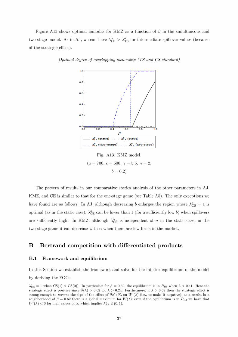
Figure A13 shows optimal lambdas for KMZ as a function of � in the simultaneous and

two-stage model. As in AJ, we can have �oCS > �oTS for intermediate spillover values (because

of the strategic e¤ect).

Optimal degree of overlapping ownership (TS and CS standard)

Fig. A13. KMZ model.

(a = 700, �c = 500, = 5:5, n = 2,

b = 0:2)

The pattern of results in our comparative statics analysis of the other parameters in AJ,

KMZ, and CE is similar to that for the one-stage game (see Table A5). The only exceptions we

have found are as follows. In AJ: although decreasing b enlarges the region where �oCS = 1 is

optimal (as in the static case), �oCS can be lower than 1 (for a su¢ ciently low b) when spillovers

are su¢ ciently high. In KMZ: although �oCS is independent of n in the static case, in the

two-stage game it can decrease with n when there are few �rms in the market.

B Bertrand competition with di¤erentiated products

B.1 Framework and equilibrium

In this Section we establish the framework and solve for the interior equilibrium of the model

by deriving the FOCs.

��CS = 1 when CS(1) > CS(0)). In particular: for � = 0:62, the equilibrium is in RIII when � > 0:41. Here thestrategic e¤ect is positive since ~�(�) > 0:62 for � > 0:24. Furthermore, if � > 0:69 then the strategic e¤ect isstrong enough to reverse the sign of the e¤ect of @x�=@� on W 0(�) (i.e., to make it negative); as a result, in aneighborhood of � = 0:62 there is a global maximum for W (�): even if the equilibrium is in RIII we have thatW 0(�) < 0 for high values of �, which implies �oTS 2 (0; 1).

37

We consider an industry with n di¤erentiated products, each produced by one �rm. The

demand for good i is given by qi = Di(p) where p is the vector of prices. Goods are (strict)

gross substitutes, @Di=@pj > 0, j 6= i. Assumptions A.2, A.3 and A.4 (with H as de�ned below)

are maintained, we replace Assumption A.1 by the following one:

Assumption 1B. For any product i, the function Di (�) is smooth whenever positive, down-

ward sloping, products are (strict) gross substitutes with @Di=@pj > 0, j 6= i, and the demand

system D (�) is symmetric with negative de�nite Jacobian.

Under Assumption 1B the demand system can be obtained from a representative consumer

with quasilinear utility and can be inverted to obtain inverse demands (see Vives 1999, pp. 144-

148). Furthermore, it follows that the demand for a variety when all �rms set the same price

(the Chamberlinian DD function) is downward sloping since the own-price e¤ect dominates the

cross-price e¤ects:

v � @Di@pi

+ (n� 1)@Dj@pi

< 0, j 6= i:

It follows that v� � @Di=@pi + �(n� 1)@Dk=@pi < 0. The innovation function is de�ned as

in Cournot. The �rm i�s pro�t now writes as

�i =

pi � c

xi + �

Pj 6=i

xj

!!Di(p)� �(xi)

and the objective function for the manager of �rm i is again: �i = �i + �Pk 6=i �k, thus

�i =

pi � c

xi + �

Pj 6=i

xj

!!Di(p)��(xi)+�

Pk 6=i

" pk � c

xk + �

Pj 6=k

xj

!!Dk(p)� �(xk)

#.

B.2 Simultaneous model

The FOCs for an interior symmetric equilibrium are

@�i@pi

= Di(p) + (pi � ci)@Di(p)

@pi+ �

Pk 6=i(pk � ck)

@Dk(p)

@pi= 0, (59)

@�i@xi

= �c0(�)Di(p)� �0(xi)� �Pk 6=i

c0(�)�Dk(p) = 0. (60)

The symmetric equilibrium is the pair (p�; x�), with q� = Di(p�) where p� = (p�; :::; p�) for all

i, that solves the system (59)-(60). The FOC for price in the symmetric equilibrium is

q� + (p� � c(Bx�))@Di(p�)

@pi+ �(n� 1)(p� � c(Bx�))@Dk(p

�)

@pi= 0.

38

Note that v < 0 ensures that p� � c(Bx�) is strictly positive for all �; the above condition can

be rewritten as

q� +(p� � c(Bx�))

p�@Di(p

�)

@pi

p�q�

Di(p�)+ �(n� 1)(p

� � c(Bx�))p�

@Dk(p�)

@pi

p�q�

Dk(p�)= 0.

Using the notation: �i = � (@Di(p�)=@pi) (p�=Di(p�)) and �ik = (@Dk(p�)=@pi) (p�=Dk(p

�)),

k 6= i, we can write

1� p� � c(Bx�)p�

�i + �(n� 1)p� � c(Bx�)

p��ik = 0.

From the above condition and from (60), a symmetric (interior) equilibrium will satisfy the

following two conditions:p� � c(Bx�)

p�=

1

�i � �(n� 1)�ik; (61)

�c0(Bx�)q�� = �0(x�). (62)

Note that the latter condition is also obtained in Cournot oligopoly.

Finally, we assume the following parallel regularity conditions to the Cournot case:

�p � @pipi�i + (n� 1)@pipj�i < 0 (63)

and

� � �p�x ��@xipi�i + (n� 1)@pjxi�i

� �@xipi�i + (n� 1)@xjpi�i

�> 0, (64)

where

�x � @xixi�i + (n� 1)@xixj�i.

Since @xixi�i = �c00(Bx�)�1 + �(n� 1)�2

�q���00(x�) and @xixj�i = �c00(Bx�) [� + � (1� �)]�q�,

it follows that

�x = �c00(Bx�)q��B � �00(x�) < 0 (65)

under Assumptions A.2 and A.3. Together conditions (63) and (64) imply that the FOCs (61)

and (62) both have a unique symmetric solution if they hold globally, and we assume that a

symmetric regular equilibrium exists.

B.2.1 Comparative statics with respect to �

In this Section we show that, as in the Cournot oligopoly model, if @x�=@� � 0, then @p�=@� > 0

(Lemma B1). Secondly, we derive the signs: sign f@x�=@�g and sign f@p�=@�g (Lemma B2).

39

Finally, we discuss conditions that identify the three regions in Bertrand competition with

product di¤erentiation.

As in the Cournot oligopoly model, we can establish

LEMMA B1 In the symmetric equilibrium, @p�

@� > 0 if @x�

@� � 0.

Proof. By totally di¤erentiating the FOC @�i=@pi = 0 with respect to � we obtain:

@pipi�i@p�

@�+ (n� 1)@pipj�i

@p�

@�+ @xipi�i

@x�

@�+ (n� 1)@xjpi�i

@x�

@�+ @�pi�i = 0.

Therefore,

@p�

@�= � 1

@pipi�i + (n� 1)@pipj�i

�@�pi�i +

�@xipi�i + (n� 1)@xjpi�i

� @x�@�

�.

Using the stability condition �p < 0, it follows that

sign

�@p�

@�

�= sign

�@�pi�i +

�@xipi�i + (n� 1)@xjpi�i

� @x�@�

�. (66)

Since @�pi�i = (n� 1)(p� � c(Bx�))@Dk(p�)=@pi > 0, we have that

@x�

@�� 0) @p�

@�> 0 when # � @xipi�i + (n� 1)@xjpi�i < 0.

Note that

@xipi�i = �c0(Bx�)@Di(p�)

@pi� �(n� 1)c0(Bx�)�@Dk(p

�)

@pi

= ��@Di(p

�)

@pi+ �(n� 1)�@Dk(p

�)

@pi

�c0(Bx�).

The expression @xjpi�i can be obtained from (59):

@xjpi�i = �c0(Bx�)�@Di(p�)

@pi� �c0(Bx�)@Dk(p

�)

@pi� �(n� 2)c0(Bx�)�@Dk(p

�)

@pi

= ���@Di(p

�)

@pi+ � (B � �) @Dk(p

�)

@pi

�c0(Bx�).

40

Using the above expression we can write

# = ��@Di(p

�)

@pi+ �(n� 1)�@Dk(p

�)

@pi+ (n� 1)

��@Di(p

�)

@pi+ � (B � �) @Dk(p

�)

@pi

��c0(Bx�)

= ��B@Di(p

�)

@pi+ (n� 1) [�� + � (B � �)] @Dk(p

�)

@pi

�c0(Bx�)

= ��B@Di(p

�)

@pi+ �(n� 1)B@Dk(p

�)

@pi

�c0(Bx�)

= �B�@Di(p

�)

@pi+ �(n� 1)@Dk(p

�)

@pi

�c0(Bx�).

Assumptions A.2 and v < 0 imply that # < 0.�

By totally di¤erentiating the FOCs with respect to � and solving for @p�=@� and @x�=@�

we obtain:@p�

@�=1

�

�@�xi�i

�@xipi�i + (n� 1)@xjpi�i

�� @�pi�i�x

(67)

and@x�

@�=1

�

�@�pi�i

�@xipi�i + (n� 1)@pjxi�i

�� @�xi�i�p

. (68)

To obtain sign f@x�=@�g and sign f@p�=@�g we next derive in turn each of the expressions

contained in equations (67) and (68). After some manipulations we can establish:

@xipi�i + (n� 1)@xjpi�i = �Bv�c0(Bx�),

@xipi�i + (n� 1)@pjxi�i = ��vc0(Bx�).

We also have that

@�xi�i = �(n� 1)c0(Bx�)�q� � 0,

@�pi�i = (n� 1)(p� � c(Bx�))@Dk(p

�)

@pi> 0.

Finally, we need the expressions for �p (the expression for �x is given by (65)). Recall that

�p � @pipi�i + (n� 1)@pipj�i. By di¤erentiating and evaluating in the symmetric equilibrium,

we obtain

@pipi�i = 2@Di(p

�)

@pi+ (p� � c(Bx�))

�@2Di(p

�)

@p2i+ �(n� 1)@

2Dk(p�)

@p2i

�

and, using that in the symmetric equilibrium @Di=@pj = @Dj=@pi and @2Di=@pj@pi = @2Dj=@pj@pi,

@pipj�i = (1 + �)@Di(p

�)

@pj+ (p� � c(Bx�))

�(1 + �)

@2Di(p�)

@pj@pi+ �(n� 2)@

2Dk(p�)

@pj@pi

�. (69)

41

Thus,

�p = v + v� �q�

v�(n� 1)

�1

n� 1@2Di(p

�)

@p2i+ �

@2Dk(p�)

@p2i(70)

+

�(1 + �)

@2Di(p�)

@pj@pi+ �(n� 2)@

2Dk(p�)

@pj@pi

��.

Therefore,

� = ��p�c00(Bx�)q��B + �00(x�)

�� �Bvv�

�c0(Bx�)

�2 .Under regularity condition � > 0, then:

sign

�@x�

@�

�= sign

�� (p� � c(Bx�)) @Dk(p

�)

@piv � �q��p

�(71)

and

sign

�@p�

@�

�= sign

��(n� 1)c0(Bx�)�q�

��Bv�c0(Bx�)

�� (n� 1)(p� � c(Bx�))@Dk(p

�)

@pi�x

�,

thus

sign

�@p�

@�

�= sign

��B�q�v�c0(Bx�) + (p� � c(Bx�))

@Dk(p�)

@pi

�xc0(Bx�)

�. (72)

Clearly, from (71) and (72), and in line with the Cournot oligopoly model: for � = 0, @x�=@� < 0

and @p�=@� > 0. Let P 0(c) be the cost pass-through coe¢ cient P 0(c) � dp�=dc; for � > 0 we

can establish the analogous to Lemmata 1 and 2:

LEMMA B2 In the symmetric equilibrium

sign

�@x�

@�

�= sign

�� � P 0(c) jvj

v2��@Dk(p

�)

@pi

�, (73)

where P 0(c) = v�=�p > 0, and

sign

�@p�

@�

�= sign fH � �Bg , (74)

where

H =@Dk(p

�)=@pi

(v�c0(Bx�))2

��c

00(Bx�)B�0(x�)

c0(Bx�)+ �00(x�)

�. (75)

Proof. Inserting the FOC with respect to the price, p�� c(Bx�) = �q�=v�, into (71) yields

sign f@x�=@�g = sign��� @Dk(p

�)

@pi

�v

v�

�� ��p

�.

By computing the total derivative of @�i=@pi = 0 with respect to the cost c, we obtain P0(c) =

42

v�=�p, and therefore (73). Using again the FOC: p�� c(Bx�) = �q�=v�, and equation (65), we

get

sign

�@p�

@�

�= sign

��B�v�c0(Bx�)�

1

v�c0(Bx�)

@Dk(p�)

@pi

��c00(Bx�)q� (�B)� �00(x�)

��.

Noting that the FOC with respect to R&D investment can be re-written as q� = �0(x�)=(�c0(Bx�)�),

and using that v�c0(Bx�) > 0, we have

sign

�@p�

@�

�= sign

��B + 1

� (v�c0(Bx�))2

@Dk(p�)

@pi

��c

00(Bx�)B�0(x�)

c0(Bx�)+ �00(x�)

��:

As in the Cournot oligopoly model we de�ne the functionH for Bertrand competition with di¤er-

entiated products as shown in equation (75). Thus, in the symmetric equilibrium: sign f@p�=@�g =

sign fH � �Bg.�

In Cournot we showed that sign f@q�=@�g = sign f�B �Hg. The reverse of the terms inside

the curly brackets is explained by the di¤erent type of competition (price/output competition)

in the two models. Assuming that �00 > 0, we can rewrite H as follows:

H =@Dk(p

�)=@pi

(v�c0(Bx�))2 �

00(x�)

��c

00(Bx�)Bx�

c0(Bx�)

�0(x�)

�00(x�)x�+ 1

�. (76)

By de�ning, as we did in the Cournot model, �(Bx�) � �c00(Bx�)Bx�=c0(Bx�) � 0, y(x�) �

�00(x�)x�=�0(x�) � 0,

�(q�; x�) � (v�c0(Bx�))2

@Dk(p�)@pi

�00(x�)> 0,

and by replacing these terms into (76) we get

H =1

�(q�; x�)

�1 +

�(Bx�)

y(x�)

�.

Note that the only di¤erence with respect to the Cournot model is that here the expression

for the relative e¤ectiveness of R&D (�) takes into account the fact that products are now

di¤erentiated. In Cournot: � = �(c0(Bx�))2=(f 0(Q�)�00(x�)); in Bertrand with di¤erentiated

products, however, the term (f 0)�1 is replaced by v� 2 (@Dk(p�)=@pi)�1.

We can proceed as in the Cournot model and de�ne the corresponding three regions: RI,

where @p�=@� > 0 and @x�=@� � 0; RII where @p�=@� > 0 and @x�=@� > 0; RIII where

@p�=@� < 0 and @x�=@� > 0.

Regarding RI, because of gross substitutes (@Dk(p�)=@pi > 0), we can have @x�=@� < 0

for all � (73). This is the case when ��p < � (@Dk(p�)=@pi) v=v�. Regarding the spillover

43

threshold between RII and RIII, note that here, as in Cournot, Assumption A.4 implies that

the equation H � �B = 0 has a unique positive solution, which again we may denote by �0.

It follows that for � > �0, @p�=@� < 0. Furthermore, RIII exists (because the threshold �0 is

strictly lower than 1) when n > H(1).

B.2.2 Welfare analysis

Welfare (with quasilinear utility) at a symmetric equilibrium is given by

W = U(q�)� c(Bx�)nq� � n�(x�),

where q� is the equilibrium output vector and U is the utility of a representative consumer,

assumed to be smooth and strictly concave (i.e., with a negative de�nite Hessian). By di¤eren-

tiating with respect to �:

W 0(�) =

�Pi

@U(q�)

@qi� nc(Bx�)

�@q�

@���nc0(Bx�)Bq� + n�0(x�)

� @x�@�.

From the maximization problem of the consumer: pi = @U(q�)=@qi, so

W 0(�) = (p� � c(Bx�))n@q�

@���nc0(Bx�)Bq� + n�0(x�)

� @x�@�.

From the FOC with respect to price: p� � c(Bx�) = �q�=v�, and from the FOC with respect

to R&D investment: �0(x�) = �c0(Bx�)q�� , thus

W 0(�) = � q�

v�n@q�

@���nc0(Bx�)Bq� � nc0(Bx�)q��

� @x�@�

= � q�

v�n@q�

@�� nc0(Bx�)q�(B � �)@x

�

@�.

From the demand de�nition, q� = Di(p�(�)) we have that @q�=@� = v (@p�=@�). Using that

B � � = (1� �)�(n� 1), we �nally may write

W 0(�) = ��v

v�

@p�

@�+ (1� �)�(n� 1)c0(Bx�)@x

�

@�

�nq�. (77)

Thus,

� in RI, where @x�=@� � 0 and @p�=@� > 0 (so @q�=@� < 0): W 0(�) < 0.

� in RII, where @x�=@� > 0 and @p�=@� > 0 (so @q�=@� < 0): W 0(�) 7 0.

� in RIII, where @x�=@� > 0 and @p�=@� < 0 (so @q�=@� > 0): W 0(�) > 0.

44

From (67), it follows that

@p�

@�=(n� 1)q�

�

��c0(Bx�)

�2�Bv� �

@Dk(p�)=@piv�

�c00(Bx�)q�B� + �00(x�)

��. (78)

Similarly, from (68), after some manipulations, we obtain

@x�

@�=(n� 1)q�(�c0(Bx�))

�

@Dk(p�)

@pi

24�0@ �p

�@Dk(p�)@pi

1A� v

v��

35 . (79)

By inserting (78) and (79) into (77) we obtain

W 0(�) =(n� 1)n q� 2

�

@Dk(p�)

@piz (80)

where

z � (c0(Bx�))2 �B(�v)@Dk(p�)=@pi

+v

v� 2�c00(Bx�)q�B� + �00(x�)

�(81)

+�c0(Bx�)

�2(1� �)�(n� 1)

�� (��p)

@Dk(p�)=@pi� v

v��

�.

Remark B1. Consider the case of independent products, @Dk(p�)=@pi = 0. If the local

monopoly problem is well-de�ned we have: (i) if � > 0, then �oTS = �oCS = 1, whereas (ii) if

� = 0, then � has no impact on total surplus or consumer surplus.

Proof. It follows immediately from equation (71) that sign f@x�=@�g > 0 for � > 0 and

@x�=@� = 0 for � = 0. Similarly, from equation (72): sign f@p�=@�g < 0 (or equivalently

sign f@q�=@�g > 0) for � > 0, while @p�=@� = @q�=@� = 0 for � = 0. Using (77), W 0(�) > 0 for

all � if � > 0, thus �oTS = 1. Since sign fCS0(�)g = sign f@q�=@�g, we also have that �oCS = 1. If

� = 0, clearly from (77), W 0(�) = 0; note that for @Dk(p�)=@pi = � = 0, FOCs do not depend

on �.�

B.3 Two-stage model

We �rst derive the FOCs and the expression for ~�(�) for the Bertrand case. We then discuss

the strategic e¤ect and welfare in Bertrand with two stages.

Interior equilibrium and threshold ~�(�). Let

' � �@Di(p�)

@pi@pipi�i + �

@Dk(p�)

@pi

�(n� 1)@pipj�i � (n� 2)@pipi�i

�.

45

Then, using (36) we can write:

@

@xip�j (x) =

�c0(Bx)

(�')�~�(�)� �

�, (82)

where

��@pipi�i � @pipj�i

� �@pipi�i + (n� 1) @pipj�i

�(83)

and

~�(�) =1

(�')

�@Di(p

�)

@pi@pipj�i � �

@Dj(p�)

@pi@pipi�i

�. (84)

The denominator of ~�(�) is positive since ' < 0:

' � �@Di(p�)

@pi@pipi�i + �

@Dk(p�)

@pi

�(n� 1)@pipj�i � (n� 2)@pipi�i

�(85)

= �@Di(p�)

@pi@pipi�i + �

@Dk(p�)

@pi

�@pipi�i + (n� 1)@pipj�i

�� �@Dk(p

�)

@pi(n� 1)@pipi�i

= �@Dk(p

�)

@pi�p � @pipi�i

�@Di(p

�)

@pi+ �(n� 1)@Dk(p

�)

@pi

�< 0.

Therefore, if@Di(p

�)

@pi@pipj�i � �

@Dj(p�)

@pi@pipi�i < 0 (86)

then ~�(�) < 0. Condition (86) is satis�ed in the case of linear and constant elasticity demand

with di¤erentiated products (see analysis below).

Finally, note that in Bertrand at the symmetric equilibrium FOCs boil down to

q� + (p� � c(Bx�))v� = 0 (87)

and

�c0(Bx�)�q� � �0(x�) + (n� 1)@�i@pj

�@p�j@xi

�= 0. (88)

Strategic e¤ect. The strategic e¤ect is

(x) � (n� 1) @@pj

�i(p�(x);x)

@

@xip�j (x). (89)

Next we show that @�i=@pj is strictly positive for � < 1. We then show that @p�j=@xi < 0 with

strategic complements price competition and � high enough, and as a result the strategic e¤ect

is negative.

46

We can write the FOC with respect to R&D as

@

@xi�i(p

�(x);x; �) + (n� 1) @@pj

�i(p�(x);x; �)

@

@xip�j (x) = 0,

and

@

@pj�i(p

�(x);x; �) = (p� � c(Bx)) @Di(p�)

@pj+ �

�q� + (p� � c(Bx)) @Dj(p

�)

@pj

�+�(n� 2)(p� � c(Bx))@Dk(p

�)

@pj,

which can be rewritten as

@

@pj�i(p

�(x);x; �) =�q�v�

�@Di(p

�)

@pj+ �

@Dj(p�)

@pj+ �(n� 2)@Dk(p

�)

@pj

�+ �q�, (90)

where we have used the FOC: (p� � c(Bx)) = �q�=v�. To show that @�i(p�(x);x; �)=@pj > 0,

we rewrite (90) as follows:

@

@pj�i(p

�(x);x; �) =�q�v�

�@Di(p

�)

@pj+ �

@Dj(p�)

@pj+ �(n� 2)@Dk(p

�)

@pj� �v�

�=

�q�v�

�@Di(p

�)

@pj+ �

@Dj(p�)

@pj+ �(n� 2)@Dk(p

�)

@pj

���@Di(p

�)

@pi+ �(n� 1)@Dk(p

�)

@pi

��.

Using now that in the symmetric equilibrium @Di=@pi = @Dj=@pj and @Di=@pj = @Dk=@pj =

@Dk=@pi for i 6= j, j 6= k, i 6= k we can rewrite the above expression as follows

@

@pj�i(p

�(x);x; �) =�q�v�

�1 + � (n� 2)� �2 (n� 1)

� @Di(p�)@pj

(91)

=�q�v�

(1� �) �@Di(p�)

@pj> 0 for � < 1.

We now show that @2�i=@xj@pi is negative or positive depending on whether � is high or

low. Note that:

@2�i@xi@pi

(x) = �c0(Bx)�@Di(p

�)

@pi+ � (n� 1)�@Dk(p

�)

@pi

�

47

and

@2�i@xj@pi

(x) = �c0(Bx)��@Di(p

�)

@pi+ �

@Dj(p�)

@pi+ � (n� 2)�@Dk(p

�)

@pi

�= �c0(Bx)

��

�@Di(p

�)

@pi+ �(n� 1)�@Dk(p

�)

@pi

�+ (1� �)�@Dk(p

�)

@pi

�.

Therefore, @2�i=@xj@pi < 0 for � high enough. From (36), we have

@

@xip�j (x) =

1

�@xipi�i@pipj�i � @xhpi�i@pipi�i

�,

where in the symmetric equilibrium, and using that p� � c(Bx) = �q�=v�,

@pipi�i(x) = 2@Di(p

�)

@pi+

��q�v�

��@2Di(p

�)

(@pi)2 + �(n� 1)@

2Dk(p�)

(@pi)2

�

and

@pipj�i(x) =@Di(p

�)

@pj+

��q�v�

��(1 + �)

@2Di(p�)

@pj@pi+ �(n� 2)@

2Dk(p�)

@pj@pi

�+ �

@Dj(p�)

@pi. (92)

Strategic complements price competition @pipj�i(x) > 0, together with the assumption �p <

0, both imply that > 0. Note also that the assumption v < 0 implies @2�i=@xi@pi < 0, and

since the expression for @2�i=@xj@pi becomes negative for � high enough, we can establish:

@p�j@xi

< 0 with strategic complements price competition and � high enough,

in which case the strategic e¤ect is negative and �rms adopt a "puppy dog" strategy (Fudenberg

and Tirole 1984): increasing xi decreases the prices of rivals because a larger xi shifts the price

best reply of �rm j inwards as @2�j=@xi@pj < 0 and also shift inwards the price best reply of

�rm i since @2�i=@xi@pi < 0. The result is that the strategic e¤ect is negative ( < 0) and we

have puppy dog investment incentives.

Welfare. From our previous analysis:

W 0(�) = (p� � c(Bx�))n@q�

@���nc0(Bx�)Bq� + n�0(x�)

� @x�@�.

The FOC with respect to x is

�0(x�) = �c0(Bx�)h� + (n� 1)!(�)

�~�(�)� �

�iq�. (93)

48

Inserting the FOCs p� � c(Bx�) = �q�=v� and (93) into the expression for W 0(�) we obtain:

W 0(�) =

�� 1

v�

@q�

@��h(1� �)� � !(�)

�~�(�)� �

�i(n� 1) c0(Bx�)@x

�

@�

�nq�. (94)

In Cournot when the strategic e¤ect is negative (i.e.,�~�(�)� �

�< 0) , the sign of the impact of

� on welfare in each region (RI, RII and RIII) is the same in the simultaneous and the two-stage

model. This is the case also with Bertrand competition and � high (puppy dog strategy).

B.4 Model speci�cations

In this section we characterize the model with linear and constant elasticity demands analogs

to AJ and CE. For each case, we �rst consider the simultaneous and then the two-stage model.

B.4.1 Linear model

Model speci�cation: main assumptions. We assume the following: Di(p) = a � bpi +

mPj 6=i pj with a; b;m > 0; this linear direct demand obtains from a representative consumer

with the following symmetric and strictly concave quadratic utility function:

U(q) = u1nPi=1

qi �1

2

u2

nPi=1

q2i + 2u3Pj 6=i

qiqj

!,

with u2 > u3 > 0, u1 > 0, and where

a =u1

u2 + (n� 1)u3,

b =u2 + (n� 2)u3

[u2 + (n� 1)u3] (u2 � u3)

and

m =u3

[u2 + (n� 1)u3] (u2 � u3).

(See Vives 1999, pp. 146-147.)

The innovation function of �rm i is ci = �c � xi � �Pj 6=i xj and the cost of investing x in

R&D is given by �(x) = ( =2)x2. Linear demand satis�es Assumption 1B, the innovation and

investment functions satisfy Assumptions A.2 and A.3. Under this model speci�cation, we have

v = �b + (n � 1)m, and v� = �b + �(n � 1)m. According to the above analysis, we impose:

v < 0, i.e. b > (n� 1)m.

49

Simultaneous model. Interior equilibrium. By solving the FOCs and using that in the

symmetric equilibrium q� = a+ vp�, we derive the symmetric interior equilibrium:

p� =v� (Ba� � �c ) + a

�

and

x� =�(�v�) (�cv + a)

�.

Second-order, stability and regularity conditions. It is straightforward to obtain that

�x = � , �p = v + v� = �2b+ (n� 1)m(1 + �), and � = �(v + v�) � vv�B� .

Because demand is linear, the regularity condition �p < 0 is implied by the assumption v <

0. We thus only have to impose the second regularity condition (64), therefore we assume

�(v + v�) > vv�B� . Second order conditions are: @pipi�i = �2b < 0, @xixi�i = � < 0 and

@pipi�i(@xixi�i)� (@xipi�i)2 > 0, which is equivalent to 2 b > [�b+ �(n� 1)�m]2.

Table B1: Linear Bertrand Model

Demand Di(p) = a� bpi +mPj 6=i pj

ci = �c� xi � �Pj 6=i xj

�(x) = ( =2)x2

v = �b+ (n� 1)mv� = �b+ �(n� 1)mS.O.C b > [�b+ �(n� 1)�m]2 =2Regularity Condition [� (v + v�) =vv�] > B�

Comparative statics on � and spillover thresholds. Recall that only RI exits if

��p < (@Dk(p�)=@pi) �(v=v�), i.e., if

� (v + v�) < m�

�v

v�

�, (95)

otherwise we can identify RII and RIII by deriving the corresponding spillover threshold. From

(73):

sign

�@x�

@�

�= sign

n�h� (v + v�)

v�v� �(n� 1)m

i�m

o.

Therefore,

if � � � (�) � m [b� (n� 1)m]�(n� 1)2(�+ 2)m2 � 4b (�+ 1=4) (n� 1)m+ 2b2

, (96)

50

then @x�=@� � 0 and @p�=@� > 0 (RI). It is easy to see that � (�) depends only on m=b and

that it is hump-shaped in m=b (with � (�) = 0 for m=b = 0 and for m=b = 1= (n� 1)).

Note that � = 0, y = 1 and � = �[b��(n�1)m]2m , so

H =m

[b� �(n� 1)m]2. (97)

Since v� < 0, H is strictly increasing in �. Thus,

sign

�@p�

@�

�= sign fH � �Bg .

It follows that:

�0 =�1 +

p4H(n� 1) + 12(n� 1) . (98)

As H is strictly increasing in , so is �0 (in AJ and KMZ �0 is independent of �).

Figures B1a and B1b depict the spillover thresholds and the three regions. The threshold

for RI and RII is given by (96), whereas the threshold for RII and RIII is given by (98). For

illustrative purposes we consider two cases that only di¤er in the number of �rms. In Figure

B1a, n = 8, and condition (95) is not satis�ed for any value of � if � is su¢ ciently high,

and consequently RII and/or RIII exist. In Figure B1b, n = 10, and condition (95) holds for

� > 0:882. Thus, for � su¢ ciently high, only RI exists irrespective of the spillover level.

Spillover thresholds and regions RI, RII and RIII8

Fig. B1a. Linear Bertrand model.

(n = 8)

Fig. B1b. Linear Bertrand model.

(n = 10)

Comparative statics on �0. Straightforward calculations show that the threshold �0(�) is

strictly decreasing in b and strictly increasing in . These results are in line with the Cournot

model.9 We also obtain that �0(�) is strictly increasing in the slope of the direct demand

8All simulations are conducted for a = 700, �c = 600, b = 1:4, m = 0:12 and = 70.9 In Cournot �0(0) is strictly increasing in b (see Table A3); recall that b is the (absolute value of the) slope of

51

with respect to rival prices, m. This follows since H has the same properties. However, H is

increasing in u3=u2 for u3=u2 low (local monopolies) and decreasing in u3=u2 for u3=u2 close

to 1 (homogenous products). Therefore �0(�) is non-monotone in u3=u2. It can also be showed

that as in AJ and the CE model, �0(0) is strictly decreasing in n (the threshold does not depend

on n in KMZ), and therefore in terms of consumer surplus it is optimal to suppress overlapping

ownership for any level of spillovers when �rm entry is insu¢ cient. In particular, this is the case

in Bertrand with linear demand when n < m =b2, in which case �0(0) > 1. More generally, the

sign of @�0(�)=@n for some � 2 (0; 1) depends on the level of � and n. Numerical simulations

show that for low or moderate values of �, @�0(�)=@n < 0, whereas for high �, @�0(�)=@n > 0

if n is su¢ ciently high.10

PROPOSITION BL1 Under the linear demand speci�cation, if � (v + v�) < m� (v=v�) then

only region RI exists. Otherwise, assume n > H(1), where H is given by (97), and let � (�)

and �0 be given, respectively, by (96) and (98). Then the following statements hold :

(i) if � � � (�) ; then @q�

@� < 0 and @x�

@� � 0 (RI);

(ii) if � (�) < � � �0 (�) ; then @q�

@� � 0 and@x�

@� > 0 (RII);

(iii) if � > �0 (�) ; then @q�

@� > 0 and @x�

@� > 0 (RIII).

We have that both � (�) and �0 (�) are increasing in � and hump-shaped in u3=u2, and @�0(0)=@n <

0.

Pro�t. Simulations show that also in Bertrand with di¤erentiated products and linear

demand, pro�t in equilibrium is strictly increasing in the degree of overlapping ownership:

��0(�) > 0.

Welfare. First, we derive the threshold, ��, above which welfare increases with � starting

from � = 0. We obtain �� from the condition W 0(0) > 0. Using (80), we only have to solve

zj�=0 = 0 for � to obtain the expression for ��. In particular, we have to solve

��Bvm

+v

v� 2 � � (n� 1)

�� (�b+ v)

m+

v

v�

�= 0,

or, equivalently,

v�2 (n� 1)(b� 2v)�2 � v�v [v� +m(n� 1)]� + v m = 0.

the inverse demand in Cournot, while it is the slope of the direct demand with respect to own price in Bertrand.10For example, for b = 1:5, m = 0:1 and = 60, @�0(�)=@n < 0 for n = 2:5, but @�0(�)=@n > 0 for n = 6 and

� > 0:87.

52

The above equation has two roots, only one of them can be positive since the denominator of

the roots is �2b(n� 1)(b� 2v) < 0. Thus, �� is given by

�� =v 2 �

pv fv(n� 1)2m2 + 2 [(4 � b) v � 2b ] (n� 1)m+ b2vg

�2b(n� 1)(b� 2v) .

Numerical simulations con�rm that the spillover thresholds satisfy �0(0) > ��.

Table B2: H and Spillover Thresholds in Linear Bertrand Model

H = m = [b� �(n� 1)m]2� (�) = m [b� (n� 1)m] =

��(n� 1)2(�+ 2)m2 � 4b (�+ 1=4) (n� 1)m+ 2b2

��� =

�v 2 �

pv fv(n� 1)2m2 + 2 [(4 � b) v � 2b ] (n� 1)m+ b2vg

�= [�2b(n� 1)(b� 2v)]

�0 =��1 +

p4H(n� 1) + 1

�= [2(n� 1)]

Comparative statics on ��. As in Cournot (in AJ, KMZ and CE), the threshold �� decreases

with n. Similarly and in line with Cournot: �� decreases with the slope of demand and increases

with the parameter of the slope for the investment cost, . Regarding product di¤erentiation:

�� is hump-shaped in u3=u2 since �� = 0 both for u3=u2 = 0 and u3=u2 = 1. Finally, also in

Bertrand �� may take values greater than 1 (so �oTS = 0 irrespective of the value of �) when there

are a few �rms in the market and (b) are su¢ ciently high (low). Note that in Figures B2a-c

we assume that parameters a; b and m are �xed as n changes. This implies that parameters

u1, u2 and u3 must change with n (see Section B.4.1). Alternatively, we assume in Figure B2d

that parameters u1, u2 and u3 are �xed (such that a = 750, b = 1:5 and m = 0:1 for n = 8),

while a, b and m change with n. Results are qualitatively the same: the thresholds in B2a and

B2d are almost the same for n equal or close to 8, while they are higher in B2d than in B2a for

two or three �rms in the market.

53

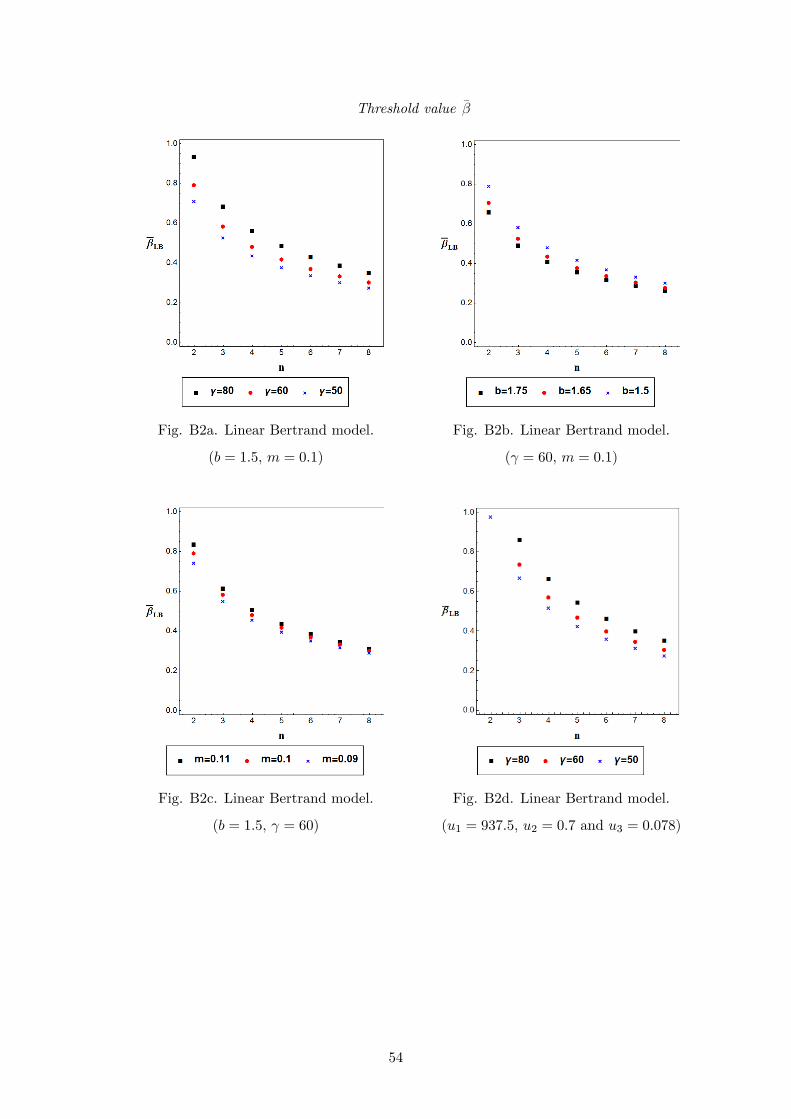
Threshold value ��

Fig. B2a. Linear Bertrand model.

(b = 1:5, m = 0:1)

Fig. B2b. Linear Bertrand model.

( = 60, m = 0:1)

Fig. B2c. Linear Bertrand model.

(b = 1:5, = 60)

Fig. B2d. Linear Bertrand model.

(u1 = 937:5, u2 = 0:7 and u3 = 0:078)

54

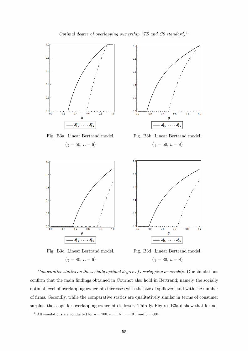
Optimal degree of overlapping ownership (TS and CS standard)11

Fig. B3a. Linear Bertrand model.

( = 50, n = 6)

Fig. B3b. Linear Bertrand model.

( = 50, n = 8)

Fig. B3c. Linear Bertrand model.

( = 80, n = 6)

Fig. B3d. Linear Bertrand model.

( = 80, n = 8)

Comparative statics on the socially optimal degree of overlapping ownership. Our simulations

con�rm that the main �ndings obtained in Cournot also hold in Bertrand; namely the socially

optimal level of overlapping ownership increases with the size of spillovers and with the number

of �rms. Secondly, while the comparative statics are qualitatively similar in terms of consumer

surplus, the scope for overlapping ownership is lower. Thirdly, Figures B3a-d show that for not

11All simulations are conducted for a = 700, b = 1:5, m = 0:1 and �c = 500.

55

too highly concentrated markets and high spillover levels, � = 1 can be optimal in terms of

total and consumer surplus. The thresholds �� and �0(0), as discussed above, decrease with n,

and the optimal degrees of overlapping ownership �oTS and �oCS, decrease with the parameter of

the slope for the investment cost, .

Optimal degree of overlapping ownership (TS and CS standard) 12

Fig. B4a. Linear Bertrand model.

( = 80, � = 0:2)

Fig. B4b. Linear Bertrand model.

( = 80, � = 0:4)

Fig. B4c. Linear Bertrand model.

( = 80, � = 0:6)

Fig. B4d. Linear Bertrand model.

( = 80, � = 0:8)

12All simulations are conducted for a = 750, b = 1:5, m = 0:1 and �c = 500.

56

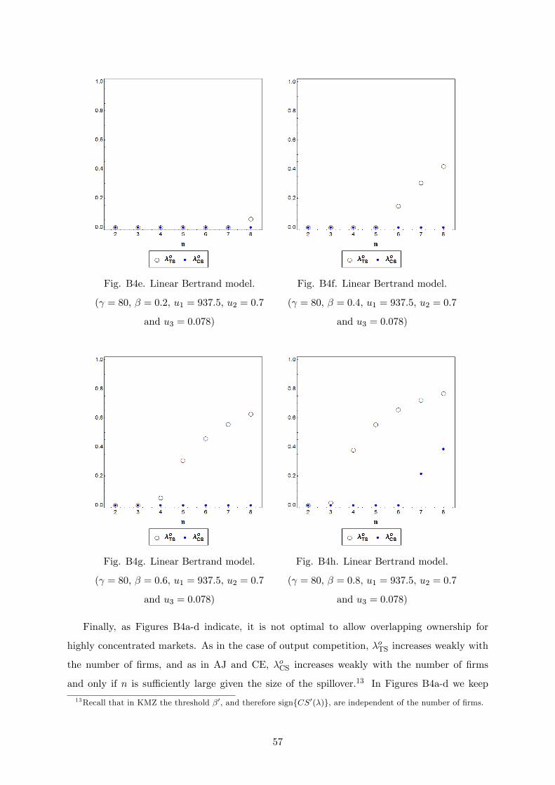
Fig. B4e. Linear Bertrand model.

( = 80, � = 0:2, u1 = 937:5, u2 = 0:7

and u3 = 0:078)

Fig. B4f. Linear Bertrand model.

( = 80, � = 0:4, u1 = 937:5, u2 = 0:7

and u3 = 0:078)

Fig. B4g. Linear Bertrand model.

( = 80, � = 0:6, u1 = 937:5, u2 = 0:7

and u3 = 0:078)

Fig. B4h. Linear Bertrand model.

( = 80, � = 0:8, u1 = 937:5, u2 = 0:7

and u3 = 0:078)

Finally, as Figures B4a-d indicate, it is not optimal to allow overlapping ownership for

highly concentrated markets. As in the case of output competition, �oTS increases weakly with

the number of �rms, and as in AJ and CE, �oCS increases weakly with the number of �rms

and only if n is su¢ ciently large given the size of the spillover.13 In Figures B4a-d we keep

13Recall that in KMZ the threshold �0, and therefore signfCS0(�)g, are independent of the number of �rms.

57

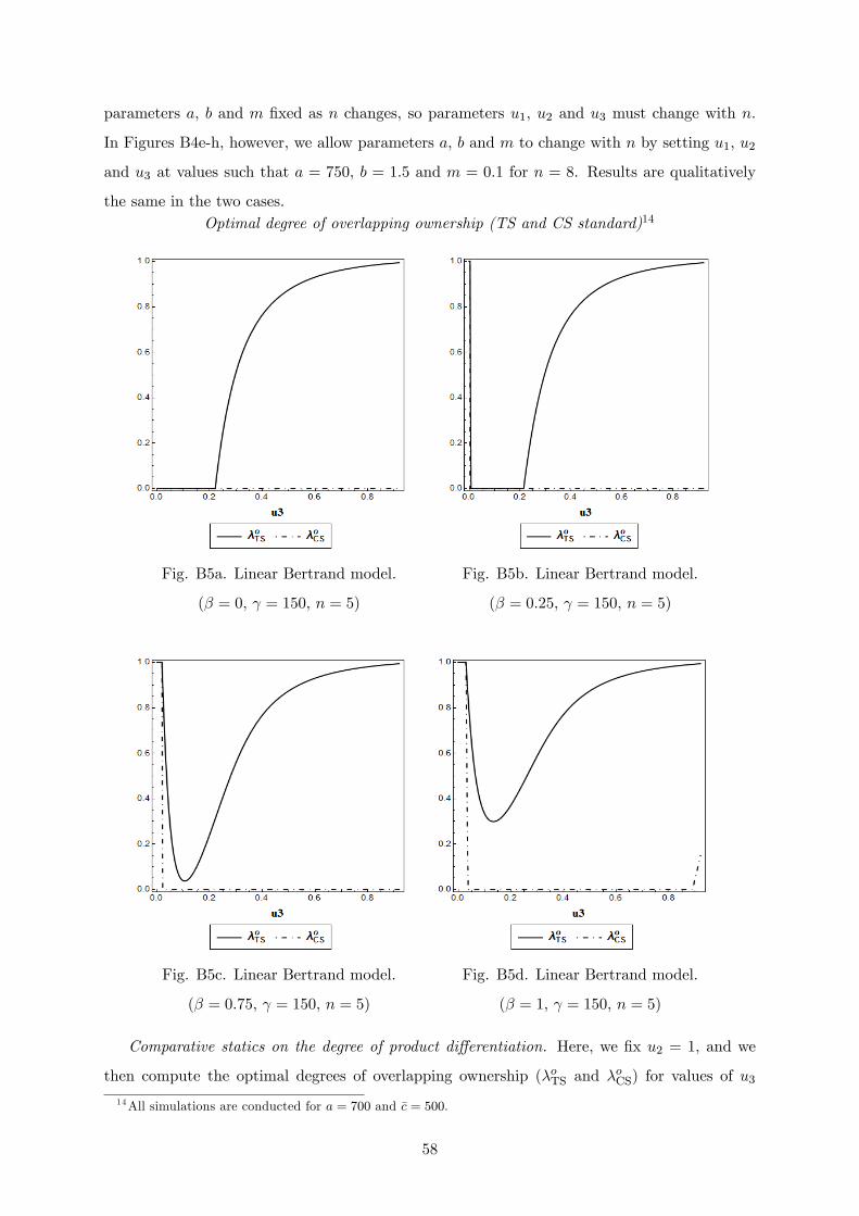
parameters a; b and m �xed as n changes, so parameters u1, u2 and u3 must change with n.

In Figures B4e-h, however, we allow parameters a, b and m to change with n by setting u1, u2

and u3 at values such that a = 750, b = 1:5 and m = 0:1 for n = 8. Results are qualitatively

the same in the two cases.Optimal degree of overlapping ownership (TS and CS standard)14

Fig. B5a. Linear Bertrand model.

(� = 0, = 150, n = 5)

Fig. B5b. Linear Bertrand model.

(� = 0:25, = 150, n = 5)

Fig. B5c. Linear Bertrand model.

(� = 0:75, = 150, n = 5)

Fig. B5d. Linear Bertrand model.

(� = 1, = 150, n = 5)

Comparative statics on the degree of product di¤erentiation. Here, we �x u2 = 1, and we

then compute the optimal degrees of overlapping ownership (�oTS and �oCS) for values of u314All simulations are conducted for a = 700 and �c = 500.

58

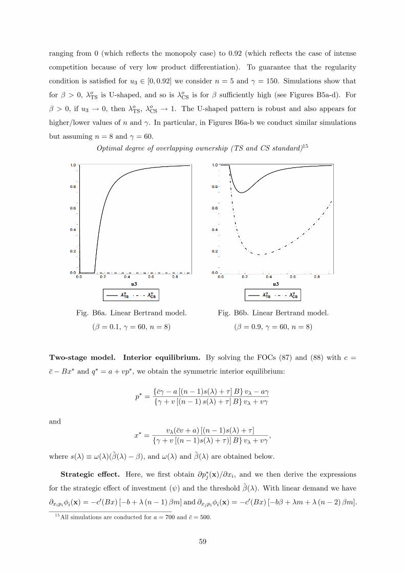
ranging from 0 (which re�ects the monopoly case) to 0:92 (which re�ects the case of intense

competition because of very low product di¤erentiation). To guarantee that the regularity

condition is satis�ed for u3 2 [0; 0:92] we consider n = 5 and = 150. Simulations show that

for � > 0, �oTS is U-shaped, and so is �oCS is for � su¢ ciently high (see Figures B5a-d). For

� > 0, if u3 ! 0, then �oTS, �oCS ! 1. The U-shaped pattern is robust and also appears for

higher/lower values of n and . In particular, in Figures B6a-b we conduct similar simulations

but assuming n = 8 and = 60.

Optimal degree of overlapping ownership (TS and CS standard)15

Fig. B6a. Linear Bertrand model.

(� = 0:1, = 60, n = 8)

Fig. B6b. Linear Bertrand model.

(� = 0:9, = 60, n = 8)

Two-stage model. Interior equilibrium. By solving the FOCs (87) and (88) with c =

�c�Bx� and q� = a+ vp�, we obtain the symmetric interior equilibrium:

p� =f�c � a [(n� 1)s(�) + � ]Bg v� � a f + v [(n� 1) s(�) + � ]Bg v� + v

and

x� =v�(�cv + a) [(n� 1)s(�) + � ]

f + v [(n� 1)s(�) + �)]Bg v� + v ,

where s(�) � !(�)(~�(�)� �), and !(�) and ~�(�) are obtained below.

Strategic e¤ect. Here, we �rst obtain @p�j (x)=@xi, and we then derive the expressions

for the strategic e¤ect of investment ( ) and the threshold ~�(�). With linear demand we have

@xipi�i(x) = �c0(Bx) [�b+ � (n� 1)�m] and @xjpi�i(x) = �c0(Bx) [�b� + �m+ � (n� 2)�m].15All simulations are conducted for a = 700 and �c = 500.

59

We also have that @pipi�i(x) = �2b and @pipj�i(x) = m (1 + �). Therefore,

@pipi�i(x)� @pipj�i(x) = �2b�m(1 + �),

@pipi�i(x) + (n� 1)@pipj�i(x) = �2b+ (n� 1)m(1 + �),

@pipj�i(x)� @pipi�i(x)� = m (1 + �) + 2b�.

Using (36) we can write

@

@xip�j (x) =

�c0(Bx)

['(�)� � (1� �) bm] ,

where = [�2b�m(1 + �)] [�2b+ (n� 1)m(1 + �)] > 0, and '(�) = � (1 + �) (n� 1)m2 +

2� (n� 2) bm � 2b2 < 0, since '(0) = �2b2 < 0, '(1) = 2(b + m) [�b+m(n� 1)] < 0 and

'0(�) > 0. Therefore,@

@xip�j (x) < 0.

From (91) we may write

@

@pj�i(p

�(x);x; �) =�q�v�

fm [1 + � (n� 2)]� b�g+ �q�

= � q�

v�m (1� �) �.

Note that (1� �)� is strictly positive for all � < 1, thus, and as expected, for � < 1:

@

@pj�i(p

�(x);x; �) > 0.

Therefore, the strategic e¤ect of investment is

� (n� 1)@�i@pj

�@p�j@xi

�= �(n� 1) q

�

v�m (1� �) �

��c0(Bx)

['(�)� � (1� �) bm]�

=�c0(Bx)

�� q

�

v�

�m(n� 1) (1� �) � ['(�)� � (1� �) bm] < 0.

We can rewrite the strategic e¤ect of investment as

= �c0(Bx)q�!(�)�~�(�)� �

�,

60

where

!(�) =m(n� 1) (1� �) �'(�)

v�> 0 and ~�(�) =

1� �'(�)

bm < 0.

Welfare. The expression for W 0(�) is given by (94). Recall that in Cournot only when the

strategic e¤ect is negative, the sign of the impact of � on welfare in each region (RI, RII and

RIII) is the same in the simultaneous and the two-stage model. The reason is that the factor

that multiplies @x�=@� in the expression for W 0(�) is positive. When the strategic e¤ect is

positive and spillovers are low, the factor is negative and as a result, welfare decreases with � in

RII, and can increase or decrease with � in RI and in RIII. In the Bertrand model with linear

demand, the strategic e¤ect is always negative, and as in Cournot, the factor that multiplies

@x�=@� is positive. (Note also that �1=v� > 0.) Therefore, the sign of the impact of � on

welfare in each region (RI, RII and RIII) is the same in the simultaneous and the two-stage

model: W 0(�) < 0 when x� decreases and p� increases with � (as in RI), W 0(�) > 0 when x�

increases and p� decreases with � (as in RIII), and W 0(�) ? 0 when x� and p� increase with �

(as in RII).

The next �gures depict the threshold ��2SLB above which welfare increases with � at � = 0.

61

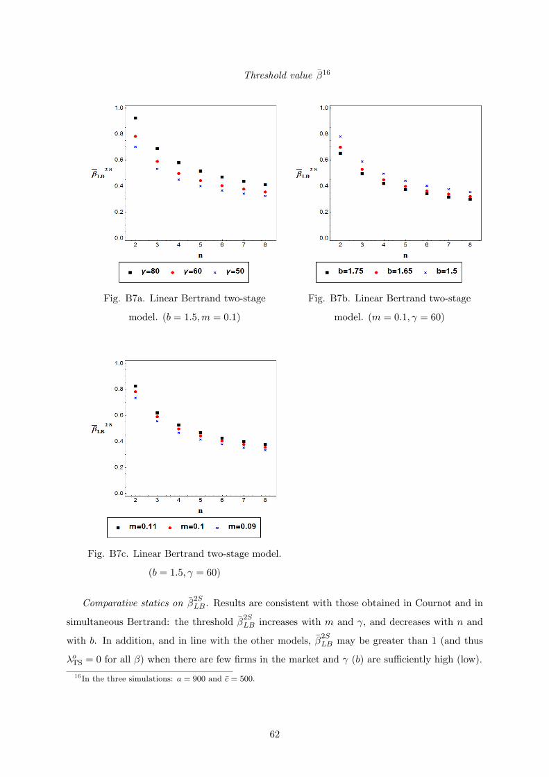
Threshold value ��16

Fig. B7a. Linear Bertrand two-stage

model. (b = 1:5;m = 0:1)

Fig. B7b. Linear Bertrand two-stage

model. (m = 0:1; = 60)

Fig. B7c. Linear Bertrand two-stage model.

(b = 1:5; = 60)

Comparative statics on ��2SLB. Results are consistent with those obtained in Cournot and in

simultaneous Bertrand: the threshold ��2SLB increases with m and , and decreases with n and

with b. In addition, and in line with the other models, ��2SLB may be greater than 1 (and thus

�oTS = 0 for all �) when there are few �rms in the market and (b) are su¢ ciently high (low).

16 In the three simulations: a = 900 and �c = 500.

62

Optimal degree of overlapping ownership (TS and CS standard)17

Fig. B8a. Linear Bertrand two-stage

model. ( = 50, n = 6)

Fig. B8b. Linear Bertrand two-stage

model. ( = 50, n = 8)

Fig. B8c. Linear Bertrand two-stage

model. ( = 80, n = 6)

Fig. B8d. Linear Bertrand two-stage

model. ( = 80, n = 8)

Comparative statics on the socially optimal degree of overlapping ownership. Results are

similar to those obtained in Cournot with two stages: �oTS increases with � and n, and when

R&D has commitment value �oTS tends to be higher than in the simultaneous model when

spillovers are high. However and unlike the Cournot model, we do not observe cases in which

�oCS > �oTS. The reason is that those cases may arise in Cournot when the strategic e¤ect is

17All simulations are conducted for a = 900, b = 1:5, m = 0:1 and �c = 500.

63

positive; in Bertrand with linear demand the strategic e¤ect is always negative. Finally, in line

with the simultaneous case, �oTS and �oCS decrease with . Note also that we do not have a

bang-bang solution for CS.

Optimal degree of overlapping ownership (TS and CS standard)18

Fig. B9a. Linear Bertrand two-stage

model. ( = 80, � = 0:2)

Fig. B9b. Linear Bertrand two-stage

model. ( = 80, � = 0:4)

Fig. B9c. Linear Bertrand two-stage

model. ( = 80, � = 0:6)

Fig. B9d. Linear Bertrand two-stage

model. ( = 80, � = 0:8)

Figures B9a-d con�rm that it is not optimal to allow overlapping ownership for highly

concentrated markets. In line with the other models, �oTS weakly increases with the number

of �rms, and �oCS increases weakly with n (only if n is su¢ ciently large given the size of the

18All simulations are conducted for a = 900, b = 1:5, m = 0:1 and �c = 500.

64

spillover).

Optimal degree of overlapping ownership (TS and CS standard)19

Fig. B10a. Linear Bertrand two-stage

model. ( = 60, � = 0:2)

Fig. B10b. Linear Bertrand two-stage

model. ( = 60, � = 0:4)

Fig. B10c. Linear Bertrand two-stage

model. ( = 60, � = 0:6)

Fig. B10d. Linear Bertrand two-stage

model. ( = 60, � = 0:8)

19All simulations are conducted for a = 900, b = 1:5, m = 0:1 and �c = 500.

65

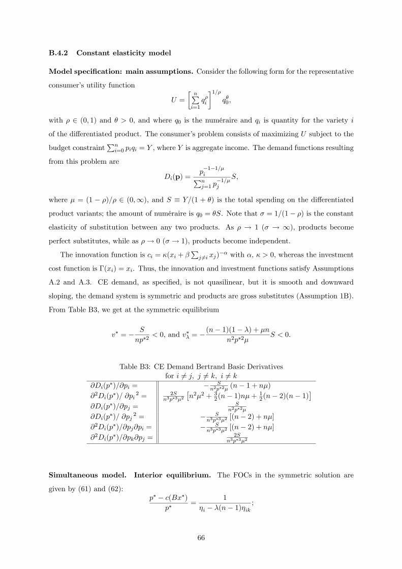
B.4.2 Constant elasticity model

Model speci�cation: main assumptions. Consider the following form for the representative

consumer�s utility function

U =

�nPi=1

q�i

�1=�q�0,

with � 2 (0; 1) and � > 0, and where q0 is the numéraire and qi is quantity for the variety i

of the di¤erentiated product. The consumer�s problem consists of maximizing U subject to the

budget constraintPni=0 piqi = Y , where Y is aggregate income. The demand functions resulting

from this problem are

Di(p) =p�1�1=�iPnj=1 p

�1=�j

S,

where � = (1 � �)=� 2 (0;1), and S � Y=(1 + �) is the total spending on the di¤erentiated

product variants; the amount of numéraire is q0 = �S. Note that � = 1=(1� �) is the constant

elasticity of substitution between any two products. As � ! 1 (� ! 1), products become

perfect substitutes, while as �! 0 (� ! 1), products become independent.

The innovation function is ci = �(xi + �Pj 6=i xj)

�� with �, � > 0, whereas the investment

cost function is �(xi) = xi. Thus, the innovation and investment functions satisfy Assumptions

A.2 and A.3. CE demand, as speci�ed, is not quasilinear, but it is smooth and downward

sloping, the demand system is symmetric and products are gross substitutes (Assumption 1B).

From Table B3, we get at the symmetric equilibrium

v� = � S

np�2< 0, and v�� = �

(n� 1)(1� �) + �nn2p�2�

S < 0.

Table B3: CE Demand Bertrand Basic Derivativesfor i 6= j; j 6= k; i 6= k

@Di(p�)=@pi = � S

n2p�2� (n� 1 + n�)@2Di(p

�)= @pi2 = 2S

n3p�3�2

�n2�2 + 3

2(n� 1)n�+12(n� 2)(n� 1)

�@Di(p

�)=@pj =S

n2p�2�

@Di(p�)= @pj

2 = � Sn3p�3�2 [(n� 2) + n�]

@2Di(p�)=@pj@pi = � S

n3p�3�2 [(n� 2) + n�]@2Di(p

�)=@pk@pj =2S

n3p�3�2

Simultaneous model. Interior equilibrium. The FOCs in the symmetric solution are

given by (61) and (62):p� � c(Bx�)

p�=

1

�i � �(n� 1)�ik;

66

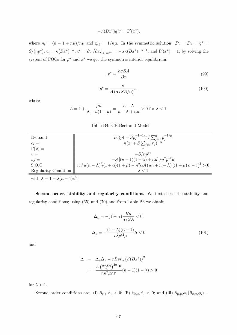
�c0(Bx�)q�� = �0(x�),

where �i = (n � 1 + n�)=n� and �ik = 1=n�. In the symmetric solution: Di = Dk = q� =

S=(np�), ci = �(Bx�)��, c0 = @ci=@xijxi=x� = ���(Bx�)���1, and �0(x�) = 1; by solving the

system of FOCs for p� and x� we get the symmetric interior equilibrium:

x� =��SA

Bn(99)

p� =�

A (��SA=n)�, (100)

where

A = 1 +�n

�� n(1 + �) =n� �

n� � + n� > 0 for � < 1.

Table B4: CE Bertrand Model

Demand Di(p) = Sp�1�1=�i =

Pnj=1 p

�1=�j

ci = �(xi + �Pj 6=i xj)

��

�(x) = xv = �S=np�2v� = �S [(n� 1)(1� �) + n�] =n2p�2�S.O.C �n4�(n� �)~�(1 + �)(1 + �)� n2�A (�n+ n� �) [(1 + �)n� � ]2 > 0Regularity Condition � < 1

with ~� = 1 + �(n� 1)�2.

Second-order, stability and regularity conditions. We �rst check the stability and

regularity conditions; using (65) and (70) and from Table B3 we obtain

�x = �(1 + �)Bn

��SA< 0,

�p = �(1� �)(n� 1)

n2p�2�S < 0 (101)

and

� = �p�x � �Bvv��c0(Bx�)

�2=

A���SAn

�2�B

n�2���(n� 1)(1� �) > 0

for � < 1.

Second order conditions are: (i) @pipi�i < 0; (ii) @xixi�i < 0; and (iii) @pipi�i (@xixi�i) �

67

(@pixi�i)2 > 0. Conditions (i) and (ii) are satis�ed:

@pipi�i = 2@Di(p

�)

@pi��q�

vL

��@2Di(p

�)

@p2i+ �(n� 1)@

2Dk(p�)

@p2i

�(102)

= �S1+2�

���n

�2�A2�+2(1� �)(1 + �)

�n�1n

�[(1� �)(n� 1) + �n]��2 < 0

and

@xixi�i = �c00(Bx�)�1 + �(n� 1)�2

�q� � �00(x�)

= ��1 + �

�

�n

�SA

�1 + �(n� 1)�2

�< 0.

Using that

@pixi�i = ����SAn

��A

�n��[(n� 1)(1� ��) + n�] ,

we have that condition (iii) is satis�ed i¤

����SAn

�2�A

�2n4 [(n� 1)(1� �) + �n]�2�� fD � Eg > 0

whereD � A3 [(���+ �+ 1)n+ �� � 1]2 [(n� 1)(1� �) + �n] �S2�3 n2

(��SA)2and E � n4�(1�

�)(n� 1)�1 + �(n� 1)�2

�(1 + �)(1 + �). Therefore, the SOC reduces to

�n4�(n� �)~�(1 + �)(1 + �)� n2�A (�n+ n� �) [(1 + �)n� � ]2 > 0,

where ~� � 1 + �(n� 1)�2.

Comparative statics on � and spillover thresholds. Recall that only RI exits (irre-

spective of the spillover level) if ��p < (@Dk(p�)=@pi) �(v=v�); replacing terms and simplifying

the condition reduces to

�n(2�� n)� (n� 1)2(1� �)2 > 0, (103)

which holds for � = 1. If (103) does not hold, then we may identify RII and RIII by deriving

the corresponding spillover threshold. From (99) we have that

@x�

@�=

2�S(n� 1)Bn [n� � + �n]2

������

2

2+ (1 + �)�� 1 + �

2

�n+

(1� �)22

��(n� 1)� �n

2

�,

which implies that

sign

�@x�

@�

�= sign

��

���2

2� (1 + �)�+ 1 + �

2

�n� (1� �)

2

2

�(n� 1)� �n

2

�.

68

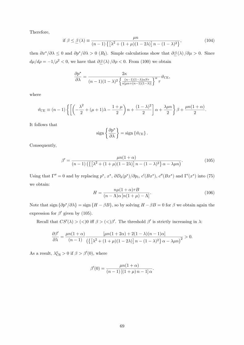
Therefore,

if � � � (�) � �n

(n� 1)���2 + (1 + �)(1� 2�)

�n� (1� �)2

, (104)

then @x�=@� � 0 and @p�=@� > 0 (RI). Simple calculations show that @� (�) =@� > 0. Since

d�=d� = �1=�2 < 0, we have that @� (�) =@� < 0. From (100) we obtain

@p�

@�=

2�

(n� 1)(1� �)2n

(n�1)(1��)�S�n[�n+(n�1)(1��)]

o��#CE,

where

#CE � (n� 1)���

��2

2+ (�+ 1)�� 1 + �

2

�n+

(1� �)22

��+

��n

2

�� +

�n(1 + �)

2.

It follows that

sign

�@p�

@�

�= sign f#CEg .

Consequently,

�0 =�n(1 + �)

(n� 1)���

�2 + (1 + �)(1� 2�)�n� (1� �)2

�� ��n

� . (105)

Using that �00 = 0 and by replacing p�; x�; @Dk(p�)=@pi; c0(Bx�), c00(Bx�) and �0(x�) into (75)

we obtain:

H =n�(1 + �)�B

(n� �)� [n(1 + �)� �] . (106)

Note that sign f@p�=@�g = sign fH � �Bg, so by solving H ��B = 0 for � we obtain again the

expression for �0 given by (105).

Recall that CS0(�) > (<)0 i¤ � > (<)�0. The threshold �0 is strictly increasing in �:

@�0

@�=�n(1 + �)

(n� 1)[�n(1 + 2�) + 2(1� �)(n� 1)�]���

�2 + (1 + �)(1� 2�)�n� (1� �)2

�� ��n

�2 > 0.As a result, �oCS > 0 if � > �0(0), where

�0(0) =�n(1 + �)

(n� 1) [(1 + �)n� 1]� .

69

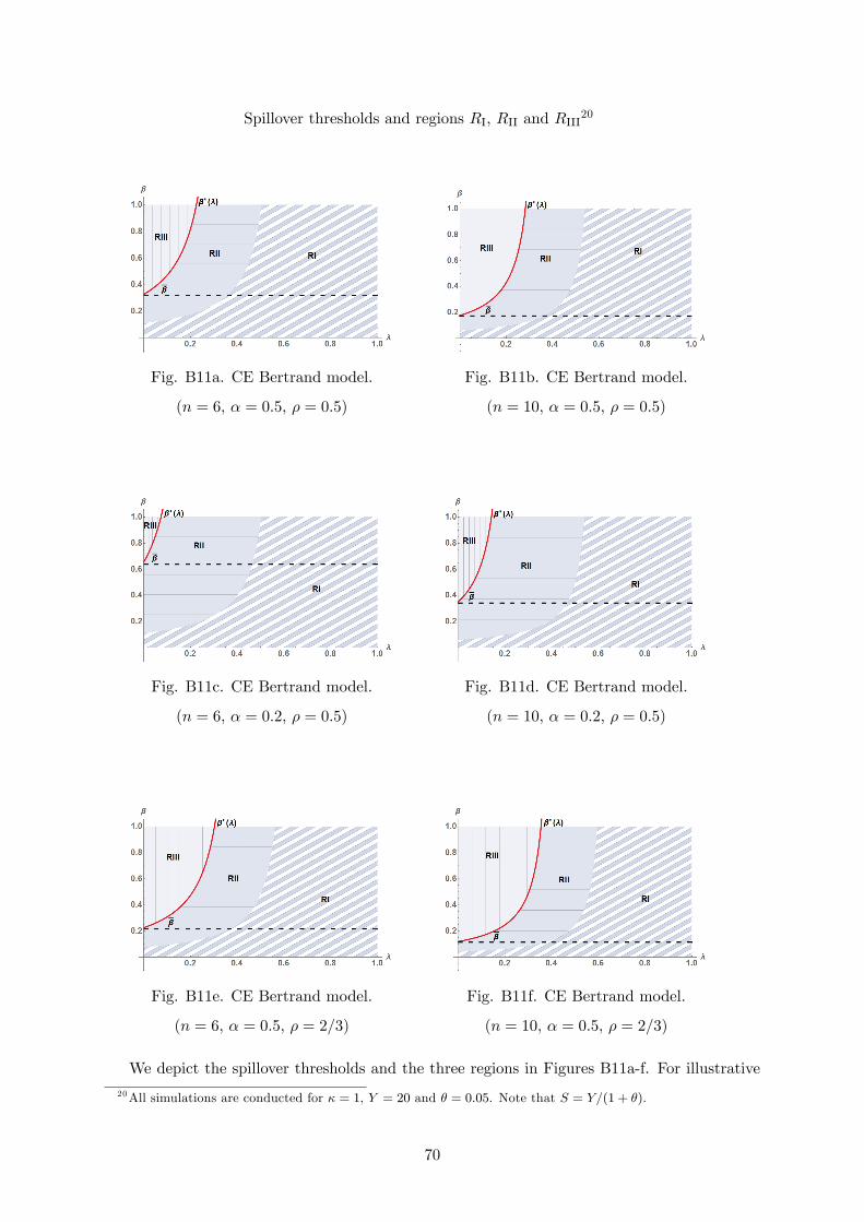
Spillover thresholds and regions RI; RII and RIII20

Fig. B11a. CE Bertrand model.

(n = 6, � = 0:5, � = 0:5)

Fig. B11b. CE Bertrand model.

(n = 10, � = 0:5, � = 0:5)

Fig. B11c. CE Bertrand model.

(n = 6, � = 0:2, � = 0:5)

Fig. B11d. CE Bertrand model.

(n = 10, � = 0:2, � = 0:5)

Fig. B11e. CE Bertrand model.

(n = 6, � = 0:5, � = 2=3)

Fig. B11f. CE Bertrand model.

(n = 10, � = 0:5, � = 2=3)

We depict the spillover thresholds and the three regions in Figures B11a-f. For illustrative

20All simulations are conducted for � = 1, Y = 20 and � = 0:05. Note that S = Y=(1 + �).

70

purposes, we consider six cases that di¤er in n, � and �. In contrast to the linear demand case,

the condition under which only RI exists for all �, which is given by (103), always holds for �

close or equal to 1. For lower values of �, RII and/or RIII may exist for � su¢ ciently high. Fig.

11a-d show how area RIII (respectively, RII) increases (decreases) with �, and illustrate that

RIII increases with n. Finally, the comparison of Fig. B11a with B11e, and B11b with B11f,

display the increase of RIII with �.

Comparative statics on �0. Straightforward calculations show that �0(�) is strictly decreasing

in � and strictly increasing in �. Thus, @�0(�)=@� < 0. As in the linear demand case, �0(0) is

strictly decreasing in n. Therefore, if �0(0) > 1 for n = 2, which holds when � > �=2, then to

have �0(0) < 1, so that �oCS > 0 when � > �0(0), the number of �rms must be su¢ ciently high

such that

n >

2(1 + �)�+ �+ 2

rh��+ 1

2

�2�+ �2 + �

i�

2(1 + �)�.

PROPOSITION BCE1 Under the CE demand speci�cation, if �n(2��n)�(n�1)2(1��)2 > 0

then only region RI exists. Otherwise, assume n > H(1), where H is given by (106), and let

� (�) and �0 be given, respectively, by (104) and (105). Then the following statements hold :

(i) if � � � (�) ; then @q�

@� < 0 and @x�

@� � 0 (RI);

(ii) if � (�) < � � �0; then @q�

@� � 0 and@x�

@� > 0 (RII);

(iii) if � > �0; then @q�

@� > 0 and @x�

@� > 0 (RIII).

We have that � (�) and �0 (�) are increasing in � and decreasing in �, and @�0(0)=@n < 0.

Pro�t. By inserting equilibrium values into the pro�t function and simplifying, we obtain:

�(�) =1

nB

�n�B � ��(n� �)(�+ 1)n� �

�S.

Simulations show that also in Bertrand with CE demand, pro�t in equilibrium is strictly in-

creasing in the degree of overlapping ownership: ��0(�) > 0.

Utility. Note that the indirect utility function in not linear in income. Thus, to solve the

�rst-best problem we have to maximize the utility function subject to the resource constraint:

Y =Pni=1 ciqi +

Pni=1 �(xi) + q0. At the symmetric equilibrium the utility function with this

constraint included is

V (�) = n1=�q� (Y � nc(Bx�)q� � nx�)� ,

71

where Y = S(1 + �). Computing V 0(�) and using the FOC 1 = �c0(Bx�)�q�, after some

manipulations we can write

V 0(�) = n1=�%��1�[S(1 + �)� nc(Bx�)q�(1 + �)� nx�] @q

�

@�� c0(Bx�)�(n� 1)(1� �)�nq�2 @x

�

@�

�,

where % � S(1 + �)� nc(Bx�)q� � nx�.

We now may obtain the threshold �� from the condition W 0(0) > 0. In particular, the

equation W 0(0) = 0 is quadratic in �, and writes as #1�2 + #2� + #3 = 0, where

#1 � � [(�+ 1)n� 1] (n� 1)2�S��(n� 1)2Z�1 + [(�+ 1)n� 1]n(1 + �)n�

,

#2 � �n(n� 1)�� [(�+ 1)n� 1] (1 + �) [�(n� 1)�+ n�] (n� 1) + S��2�(n� 1)2Z�1

+ [(�+ 1)n� 1]2�(n� 1)�2 � (1 + �)(n� 1)�+ n�(1 + �)

�o,

and

#3 � �n2�(�+ 1) [(�+ 1)n� 1] f[(1 + �)�� �]n+ �g ,

with

Z � �S(n� 1)[(�+ 1)n� 1]n .

The threshold �� is given by the positive root:

�� =�#2 +

q#22 � 4#1#32#1

.

Table B5: H and Spillover Thresholds in CE Bertrand Model

H = n�(1 + �)�B= f(n� �)� [n(1 + �)� �]g� (�) = �n=

�(n� 1)

���2 + (1 + �)(1� 2�)

�n� (1� �)2

��� =

��#2 +

q#22 � 4#1#3

�= (2#1)

�0 = �n(1 + �)=�(n� 1)

����2 + (1 + �)(1� 2�)

�n� (1� �)2

�� ��n

��

72

Threshold value ��

Fig. B12a.CE Bertrand model. Fig. B12b. CE Bertrand model.

Comparative statics on ��. We observe in Fig. 12a,b that �� decreases with � and �. The

threshold as in the previous cases decreases with n and may take values greater than 1 (so

�oTS = 0 irrespective of the value of �) when there are few �rms in the market. Note that we

use notation �oTS with subscript TS even though we refer to utility V .

Comparative statics on the socially optimal degree of overlapping ownership. Simulation

results are in line with previous �ndings: the socially optimal level of overlapping ownership

increases with the size of spillovers (see Figures B13a-d) and with the number of �rms (see

Figures B14a-d).

73

Optimal degree of overlapping ownership (TS and CS standard)21

Fig. B13a. CE Bertrand model.

(� = 0:5, � = 0:5, n = 6)

Fig. B13b. CE Bertrand model.

(� = 0:5, � = 0:5, n = 8)

Fig. B13c. CE Bertrand model.

(� = 0:75, � = 0:5, n = 6)

Fig. B13d. CE Bertrand model.

(� = 0:5, � = 2=3, n = 6)

21All simulations are conducted for � = 1, Y = 20 and � = 0:05.

74

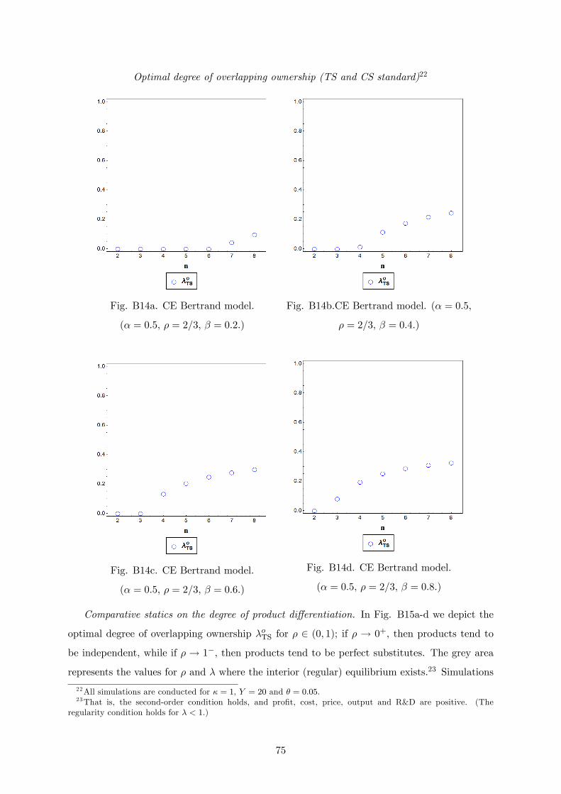
Optimal degree of overlapping ownership (TS and CS standard)22

Fig. B14a. CE Bertrand model.

(� = 0:5; � = 2=3, � = 0:2.)

Fig. B14b.CE Bertrand model. (� = 0:5;

� = 2=3, � = 0:4.)

Fig. B14c. CE Bertrand model.

(� = 0:5; � = 2=3, � = 0:6.)

Fig. B14d. CE Bertrand model.

(� = 0:5; � = 2=3, � = 0:8.)

Comparative statics on the degree of product di¤erentiation. In Fig. B15a-d we depict the

optimal degree of overlapping ownership �oTS for � 2 (0; 1); if � ! 0+, then products tend to

be independent, while if � ! 1�, then products tend to be perfect substitutes. The grey area

represents the values for � and � where the interior (regular) equilibrium exists.23 Simulations

22All simulations are conducted for � = 1, Y = 20 and � = 0:05.23That is, the second-order condition holds, and pro�t, cost, price, output and R&D are positive. (The

regularity condition holds for � < 1.)

75

show that for � > 0, �oTS increases towards 1 when � ! 1. However, �oTS is not U-shaped; the

reason is that the monopoly case is not well de�ned with CE demand: when �! 0, the price p

tends to in�nity, and therefore the output q tends to zero.

Optimal degree of overlapping ownership24

Fig. B15a. CE Bertrand model.

(� = 0:5, � = 0:25, n = 6)

Fig. B15b. CE Bertrand model.

(� = 0:5, � = 0:5, n = 6)

Fig. B15c. CE Bertrand model.

(� = 0:5, � = 0:75, n = 6)

Fig. B15d. CE Bertrand model.

(� = 0:5, � = 1, n = 6)

24All simulations are conducted for � = 1, Y = 20 and � = 0:05.

76

Two-stage model. Interior equilibrium. The interior equilibrium is characterized by the

two FOCs (87) and (88), which at the symmetric equilibrium can be written as follows

q� + (p� � c(Bx�))v� = 0

�c0(Bx�)�q� � 1 + = 0.

Next we derive the strategic e¤ect, � (n� 1)(@�i=@pj)(@p�j=@xi).

Strategic e¤ect. The expression for @�i=@pj , which is strictly positive for � < 1, is given by

(91). The expression for @p�j=@xi is computed in (82): @p�j=@xi = � (c0(Bx)=) (�')

�~�(�)� �

�.

By inserting equilibrium values into the de�nition of , given in equation (83), we get

=f(n� 1) [(1 + �)n+ �] + 1g (��SA=n)4� (n� 1)S2A4(1� �)2

n4 [(n� 1)(1� �) + �n]�2�4 > 0.

The term ' is de�ned in (85). By replacing @pipi�i, given by (102), �p given by (101), and

@Di(p�)=@pi and @Dk(p�)=@pi provided in Table B3, into ' we obtain

' = �A4���SAn

�4�(n� 1)(1� �) [n(1 + �) + �]S2

n4�4�2< 0. (107)

To obtain ~�(�) we �rst have to calculate @pipj�i, which using equation (92) and Tables B3 and

B4 can be shown to be

@pipj�i =�(1� �)S

[(n� 1)(1� �) + n�]�p2n2 .

As a result we have that

@Di(p�)

@pi@pipj�i � �

@Dj(p�)

@pi@pipi�i = �

A4���SAn

�4�(1� �)S2

n4�4�2, (108)

which is strictly negative for � < 1. By inserting (107) and (108) into (84), and simplifying, we

get

~�(�) = � 1

(n� 1) [(1 + �)n+ �] < 0.

Consequently, the strategic e¤ect is:

= � q�

v�(n� 1)(1� �)�@Di(p

�)

@pj

��c

0(Bx�)

(�')(~�(�)� �)

�.

Let

!(�) =

@Di(p�)

@pj(n� 1)(1� �)�'v�

> 0,

77

then the strategic e¤ect is shown to be negative:

= �c0(Bx�)q�!(�)�~�(�)� �

�< 0.

78