CONTINUOUS STATE DYNAMIC PROGRAMMING VIANONEXPANSIVE APPROXIMATION

JOHN STACHURSKI

ABSTRACT. This paper studies fitted value iteration for contin-uous state numerical dynamic programming using nonexpansivefunction approximators. A number of approximation schemes arediscussed. The main contribution is to provide error bounds forapproximate optimal policies generated by the value iteration al-gorithm. Journal of Economic Literature Classifications: C61, C63

1. INTRODUCTION

In dynamic programming, Bellman’s principle of optimality per-mits computation of optimal policies from the relevant value func-tion, denoted below by v∗. When no analytical representation of v∗

is available an approximation can be obtained numerically throughvalue iteration, which involves iterating the Bellman operator T onsome initial function v.1 Under mild assumptions T is supremum-norm contracting, and the resulting sequence (Tnv)∞

n=1 convergesgeometrically to v∗.

If the state space is infinite, one cannot in general implement thefunctions Tv, T2v, . . . , Tnv on a computer. One feasible alternativeis discretization, where the state space is replaced with a finite grid,and the original model with a “similar” model which evolves on

Date: August 3, 2007.Key words and phrases. Numerical dynamic programming, nonexpansive

approximation.This paper has benefitted from the comments of an anonymous referee, finan-

cial support from Australian Research Council Grant DP0557625 and the Mu-rata Science Foundation, and from helpful discussions with Takashi Kamihigashi,Kazuo Nishimura, Kevin Reffett and Rabee Tourkey.

1For background see the excellent survey of Rust (1996).1

2 JOHN STACHURSKI

this grid. A second is fitted value iteration, a standard algorithm forwhich is

initialize v;1

repeat2

evaluate Tv at finite set of grid points {xi};3

use the values to construct an approximation w ∈ F of Tv;4

set v = w;5

until a suitable stopping rule is satisfied ;6

compute an approximate optimal policy using v in place of v∗;7

Here F is a class of functions with finite parametric representa-tion. The map v 7→ w is in effect an approximate Bellman operatorT, and fitted value iteration is equivalent to iteration with T in placeof T.2

Popular architectures for constructing the approximation w of Tvin line 4 include Chebychev polynomials, cubic splines and neuralnets. These architectures are popular because they are often able toaccurately represent Tv with relatively few grid points. However, itshould be recalled that the ultimate objective is not to minimize thedistance between w and Tv. Rather it is to minimize some measureof distance between the optimal policy and the approximate opti-mal policy computed from Tnv. In particular, attention must be paidto whether or not the approximation scheme interacts well with theiteration scheme needed to compute the fixed point v∗. A scheme

2Aside from discretization and fitted value iteration, numerous alternative tech-niques have been proposed for numerical dynamic programming. They includea variety of perturbation and projection methods which act directly on the Eulerequation. A comparison of alternative methods for the stochastic optimal growthmodel is available in Aruoba, Fernandez-Villaverde and Rubio-Ramirez (2006).Our study treats a general dynamic programming problem where Euler equationsdo not necessarily exist.

NONEXPANSIVE APPROXIMATION 3

which represents the function Tv well at each iteration may in factstill lead to poor dynamic properties for the sequence (Tnv).3

At issue is the lack of compatibility between the sup-norm con-traction property of T—which drives convergence of (Tnv)∞

n=1 tov∗—and the potentially expansive properties of the approximationoperator. To clarify this point, let us decompose T into the actionof two operators L and T: First T is applied to v—in practice Tv isevaluated only at finitely many points—and then an approximationoperator L sends the result into w = Tv ∈ F . Thus, T = L ◦ T. As Tis a contraction, T = L ◦ T is contracting whenever L is, but L is notgenerally contracting.

In the present paper we pursue a suggestion of Gordon (1995),restricting attention to approximation architectures such that L isnonexpansive with respect to the sup-norm; from which it followsthat the composition T := L ◦ T is a contraction mapping. We ex-ploit the contractiveness of T to obtain a general set of error boundsfor approximate optimal policies which apply to any nonexpansiveapproximation architecture. Our focus is on structures suitable foreconomic applications.4

We pay special attention to the case where L sends functions intopiecewise constant functions—a kind of nonexpansive approxima-tor. Iteration with L ◦ T provides an algorithm that can be thoughtof as combining aspects of discretization and fitted value iteration.Compared to the common practice of one-off discretization onto a fi-nite grid, the algorithm is simple to program, preserves and exploits

3As approximation errors are compounded at each iteration, limn→∞ Tnv maydeviate substantially from limn→∞ Tnv = v∗; in fact the sequence may fail to con-verge at all. See, for example, Tsitsiklis and Van Roy (1996, Section 4), which givesan example of divergence under least-squares approximation.

4Following Gordon (1995), Drummond (1996) investigated adding penaltiesto the derivatives of function approximators in order to prevent sup-norm ex-pansiveness (overshooting). Guestrin et al. (2001) study nonexpansive approxi-mations in factored Markov Decision Processes. See also Tsitsiklis and Van Roy(1996), who provided error bounds for optimal policies when the state and actionspaces are finite.

4 JOHN STACHURSKI

information about the model primitives between grid points, admitsthe use of adaptive grids, and is always nonexpansive.

A third contribution of this paper is to investigate the expansive-ness of shape-preserving function approximators. Previously, Juddand Solnick (1994) highlighted the computational advantages of suchapproximators, where the “shapes” of greatest interest are mono-tonicity and convexity (or concavity). We show that a certain classof shape-preserving quasi-interpolants popular in computer aideddesign are also nonexpansive.

Within the economic literature, a number of studies have beenmade of approximation architectures which turn out to be nonex-pansive. Judd and Solnick (1994) noted that a class of spline inter-polants preserve the contraction property of T, and exploited thisfact in their discussion of errors. Santos and Vigo-Aguiar (1998) con-sidered a finite element method using piecewise affine functions.They also observed that their approximation scheme preserves thecontraction property of T, and these ideas were subsequently ex-tended by Gruen and Semmler (2004). Rust (1997) studies a randomdiscretized Bellman operator which is a probability one contraction.The present paper unifies and generalize some of these ideas.

Section 2 formulates the dynamic programming problem. Sec-tion 3 discusses nonexpansive approximation schemes. Section 4states results, Section 5 looks at applications, and Section 6 givesproofs.

2. FORMULATION OF THE PROBLEM

If (U, d) is a metric space, then B(U) denotes the Borel subsets ofU and bB(U) is the bounded Borel measurable functions from U toR. For f ∈ bB(U), let ‖ f ‖ := supx∈U | f (x)| denote the supremumnorm. A map M : bB(U) → bB(U) is called nonexpansive if

(1) ‖Mw− Mw′‖ ≤ ‖w− w′‖ ∀w, w′ ∈ bB(U)

and a contraction of modulus ρ if there exists a ρ ∈ [0, 1) with

(2) ‖Mw− Mw′‖ ≤ ρ‖w− w′‖ ∀w, w′ ∈ bB(U)

NONEXPANSIVE APPROXIMATION 5

Let M1 and M2 map bB(U) to itself. Note that if M1 is a contractionof modulus ρ and M2 is nonexpansive, then M2 ◦ M1 is a contractionof modulus ρ. (In much of what follows we write the compositionM2 ◦ M1 more simply as M2M1, and similarly for other composi-tions.)

Consider an infinite horizon stochastic dynamic programming prob-lem with state space S, action space A (both Borel subsets of finite-dimensional Euclidean space) and a correspondence Γ mapping Sinto B(A), with Γ(x) interpreted as the set of feasible actions at statex. Given S, A and Γ, define

gr Γ := {(x, u) ∈ S× A : u ∈ Γ(x)}

This collection of points (the graph of Γ) is called the set of all feasiblestate/action pairs. A “reward function” r sends gr Γ into R, ρ ∈ (0, 1)is a discount factor, and M(x, u; dy) is a distribution over S for eachfeasible state/action pair (x, u) ∈ gr Γ. Here M(x, u; dy) should be beinterpreted as the conditional distribution of Xt+1 when the currentstate Xt = x and the current action Ut = u.5 For example, supposethe future state is determined according to

(3) Xt+1 = F(Xt, Ut, Wt+1) WtIID∼ G(dz)

Then M(x, u; dy) is the distribution of F(x, u, W) when W ∼ G, and,for arbitrary integrable w : S → R,

(4)∫

w(y)M(x, u; dy) =∫

w[F(x, u, z)]G(dz)

The system evolves as follows. At the start of time, the agent ob-serves X0 = x0 ∈ S, where x0 is some fixed initial condition, andthen chooses action U0 ∈ Γ(X0) ⊂ A. After choosing U0, the agentreceives reward r(X0, U0). The next state X1 is now drawn accordingto distribution M(X0, U0; dy) and the process repeats.

Let Π denote the set of all measurable functions π : S → A withπ(x) ∈ Γ(x) for all x ∈ S. We refer to Π as the set of feasible policies.

5By a distribution on S is meant a probability measure on (S, B(S)). In addition,(x, u) 7→ M(x, u; B) is required to be measurable, ∀B ∈ B(S).

6 JOHN STACHURSKI

Each π ∈ Π and initial condition x0 ∈ S defines a Markov process(Xt)t≥0, where X0 is set equal to x0, and then Xt+1 ∼ M(Xt, π(Xt); dy).

Let Px0π be the joint distribution on sequence space (S∞,⊗∞

n=1B(S))induced by (Xt)t≥0, and let Ex0

π be the expectation operator corre-sponding to Px0

π . Define a map Π× S 3 (π, x0) 7→ vπ(x0) ∈ R by

(5) vπ(x0) := Ex0π

[∞

∑t=0

ρtr(Xt, π(Xt))

]Thus vπ(x0) is the value of following the policy π when starting atinitial condition x0. The value function v∗ : S → R is

(6) v∗(x0) := supπ∈Π

vπ(x0) (x0 ∈ S)

Existence of v∗ as a well defined function follows from the existenceof suprema for bounded subsets of R (see Assumption 2.1 below). Apolicy π∗ ∈ Π is called optimal if it attains the supremum in (6) forevery x0 ∈ S (equivalently, vπ∗ = v∗ on S).

Assumption 2.1. The map r is continuous and bounded on gr Γ,while Γ is continuous, nonempty and compact valued. Further,

(7) (x, u) 7→∫

w(y)M(x, u; dy)

is continuous as a map from gr Γ to R whenever w is bounded andcontinuous on S.

The continuity assumption in (7) is a version of the so-called Fellerproperty.6 In the case of the transition rule in (3) and (4), continuity of(7) holds whenever (x, u) 7→ F(x, u, z) is continuous for all z. UnderAssumption 2.1 the following optimality result obtains.7

Theorem 2.1. The value function v∗ is continuous, and is the unique func-tion in bB(S) which satisfies

(8) v∗(x) = supu∈Γ(x)

{r(x, u) + ρ

∫v∗(y)M(x, u; dy)

}(x ∈ S)

6See, for example, Stokey, Lucas and Prescott (1989, Chapter 8).7See, for example, Hernandez-Lerma and Lasserre (1999, Section 8.5).

NONEXPANSIVE APPROXIMATION 7

If π∗ is an element of Π and

(9) v∗(x) = r(x, π∗(x)) + ρ∫

v∗(y)M(x, π∗(x); dy) (x ∈ S)

then π∗ is optimal. At least one such optimal policy π∗ ∈ Π exists. Con-versely, if π∗ is an optimal policy then it satisfies (9).

Two kinds of contraction mappings are used to study the optimal-ity results. First, let Tπ : bB(S) → bB(S) be defined for all π ∈ Πby

Tπw(x) = r(x, π(x)) + ρ∫

w(y)M(x, π(x); dy) (x ∈ S)

Further, let T : bB(S) → bB(S) be defined by

Tw(x) = supu∈Γ(x)

{r(x, u) + ρ

∫w(y)M(x, u; dy)

}(x ∈ S)

The second operator T is usually called the Bellman operator. In viewof Theorem 2.1, v∗ is the unique fixed point of T in bB(S).

It is well-known that for every π ∈ Π, the operator Tπ is a con-traction on (bB(S), ‖ · ‖) of modulus ρ. The unique fixed point of Tπ

in bB(S) is vπ, where the definition of vπ is given in (5). In addition,Tπ is monotone on bB(S), in the sense that if w, w′ ∈ bB(S) andw ≤ w′, then Tπw ≤ Tπw′.8 Similarly, the Bellman operator is also acontraction of modulus ρ; and monotone on bB(S).9

3. THE APPROXIMATION OPERATOR

To carry out fitted value iteration we use an approximation oper-ator L which maps bB(S) into a collection of functions F ⊂ bB(S).In general, L constructs an approximation Lv ∈ F to v ∈ bB(S)according to a sample {v(xi)}k

i=1 of evaluations of v on grid points{xi}k

i=1 ⊂ S. As discussed in the introduction, we focus on archi-tectures with the property that L is nonexpansive with respect to the

8Inequalities such as w ≤ w′ are pointwise inequalities on S.9These results are standard. See, for example, Puterman (1994), Stokey, Lucas

and Prescott (1989) or Hernandez-Lerma and Lasserre (1999).

8 JOHN STACHURSKI

sup norm:

(10) ‖Lv− Lw‖ ≤ ‖v− w‖ ∀ v, w ∈ bB(S)

In this section we discuss examples of approximation operators withthe nonexpansive property. The discussion is largely expository, al-though the observation that Schoenberg’s variation diminishing op-erator is nonexpansive appears to be new.

Example 3.1. (Piecewise constant approximation) An elementaryapproximation architecture is provided by piecewise constant ap-proximation. Suppose that {xi}k

i=1 is a sequence of grid points in S,and that {Ji}k

i=1 is a partition of S with xi ∈ Ji for each i, Jm ∩ Jn = ∅when m 6= n, and S = ∪k

i=1 Ji. For any function v : S → R, set

Lv(x) = v(xi) ∀ x ∈ Ji

Thus Lv takes only finitely many values. Moreover, L is nonexpan-sive. To see this, pick any w, v ∈ bB(S) and any x ∈ S. Without lossof generality, suppose that x ∈ Jm. Then

|Lw(x)− Lv(x)| = |w(xm)− v(xm)| ≤ sup1≤i≤k

|w(xi)− v(xi)|

(11) ∴ ‖Lw− Lv‖ ≤ sup1≤i≤k

|w(xi)− v(xi)| ≤ ‖w− v‖

Iteration with T = LT provides an implementation of discretizationfor dynamic programs that has several theoretical and practical ad-vantages over traditional discretization. The ideas are discussed indetail in Section 5, and applied to Samuelson’s (1971) commoditypricing model.

Example 3.2. (Kernel averagers) Kernel-based approximators haveattracted much attention in recent years, partly because they pos-sess good properties in high-dimensional state spaces. One of thesemethods is the kernel averager, which can be represented by an ex-pression of the form

(12) Lv(x) = ∑ki=1 Kh(xi − x)v(xi)

∑ki=1 Kh(xi − x)

NONEXPANSIVE APPROXIMATION 9

Here the kernel Kh is a nonnegative mapping from S → R such asthe radial basis function e−‖·‖/h. The value of the kernel decays tozero as x diverges from xi. Thus, Lv(x) is a convex combination ofthe observations v(x1), . . . , v(xk) with larger weight being given tothose observations v(xi) for which xi is close to x.10

The operator L in (12) is easily seen to be nonexpansive on bB(S):Pick any x ∈ S, and let λ(x, i) := Kh(xi − x)/ ∑k

j=1 Kh(xj − x). Using

∑ki=1 λ(x, i) = 1, we have

|Lw(x)− Lv(x)| =∣∣∣∣∣ k

∑i=1

λ(x, i)(w(xi)− v(xi))

∣∣∣∣∣≤

k

∑i=1

λ(x, i)|w(xi)− v(xi)| ≤ sup1≤i≤k

|w(xi)− v(xi)|

Since x is arbitrary the claim in the lemma holds.

Example 3.3. (Continuous piecewise linear interpolation) A com-mon form of approximation in dynamic programming is piecewiselinear (piecewise affine) spline interpolation.11 To describe a gen-eral set up, let {xi}k

i=1 be a finite subset of S ⊂ Rd with the prop-erty that the convex hull of {xi}k

i=1 equals S, and let T be a trian-gularization of S relative to the nodes {xi}k

i=1. In other words, T

is a partition of S into a finite collection of non-overlapping, non-degenerate simplexes, where, for each ∆ ∈ T , the set of vertices{ζi}d+1

i=1 ⊂ {xi}ki=1.12

Each x ∈ ∆ can be represented uniquely by its barycentric coordi-nates relative to ∆:

x =d+1

∑i=1

λ(x, i)ζi, where λ(x, i) ≥ 0 andd+1

∑i=1

λ(x, i) = 1

10The smoothing parameter h controls the weight assigned to more distantobservations.

11See, for example, Santos and Vigo-Aguiar (1998) and Munos and Moore(1999).

12A simplex is called non-degenerate if it has positive measure in Rd.

10 JOHN STACHURSKI

For v ∈ bB(S) we define the interpolation operator L by

Lv(x) =d+1

∑i=1

λ(x, i)v(ζi)

Direct calculations show that if v, w ∈ bB(S), then at x we have

|Lw(x)− Lv(x)| ≤ sup1≤i≤d+1

|w(ζi)− v(ζi)| ≤ ‖w− v‖

Since x is arbitrary, L is clearly nonexpansive.

Example 3.4. (Schoenberg’s variation diminishing operator) In awell-known study, Judd and Solnick (1994) emphasize the advan-tages of fitted value iteration with shape-preserving approximators;the shapes of greatest interest are monotonicity and convexity, andapproximators which preserve them not only incorporate knownstructure from the target function in approximation, they also allowmonotonicity and convexity to be exploited in the optimization stepof the value iteration algorithm.13

Judd and Solnick discuss several univariate shape-preserving ar-chitectures, including (nonsmooth) univariate piecewise linear inter-polants and (smooth) Schumaker splines. Here we describe a furtherclass of smooth, shape-preserving univariate approximators knownas Schoenberg variation diminishing splines.

To construct the operator we set S = [a, b] ⊂ R, and in place of astandard grid we use for each d ∈ N a d + 1-regular knot sequence(ti)k+d+1

i=1 , which satisfies

a = t1 = · · · = td+1 < td+2 < · · · < tk+1 = · · · = tk+d+1 = b

Here d is the order of the spline, so that, for example, d = 3 corre-sponds to a cubic spline. The Schoenberg splines are built using k

13Monotonicity is exploited as follows: In monotone programs the optimal ac-tion is often increasing in the state, in which case one need not search for optimalactions in that subset of the action space which is dominated by the optimal actionat a lower state. The importance of convexity in optimization needs no illustrationhere.

NONEXPANSIVE APPROXIMATION 11

basis functions which are known as B-splines. The latter are definedrecursively by

Bi,0 := 1[ti,ti+1), i = 1, . . . , k

and then, i = 1, . . . , k,

Bi,d(x) :=x − ti

ti+d − tiBi,d−1(x) +

ti+d+1 − xti+d+1 − ti+1

Bi+1,d−1(x)

where in the definition we are using the convention that 0/0 = 0.For fixed d the basis functions B1,d, . . . , Bk,d are linearly independentand satisfy ∑k

i=1 Bi,d = 1S. Their span is often denoted by Sd:

Sd :=

{k

∑i=1

αiBi,d : (α1, . . . , αk) ∈ Rk

}

Clearly Sd ⊂ bB(S). Setting t∗i := (ti+1 + · · · + ti+d)/d, Schoen-berg’s variation diminishing operator is given by

L : bB(S) 3 v 7→k

∑i=1

v(t∗i )Bi,d ∈ Sd

It is well-known that L preserves monotonicity and convexity (con-cavity) in v.14 It is easy to see that L is also nonexpansive on bB(S).To check this, pick any v, w ∈ bB(S), and let x ∈ S.

|Lw(x)− Lv(x)| ≤k

∑i=1

Bi,d(x)|w(t∗i )− v(t∗i )|

≤k

∑i=1

Bi,d(x) sup1≤j≤k

|w(t∗j )− v(t∗j )|

Using ∑ki=1 Bi,d(x) = 1, we have

|Lw(x)− Lv(x)| ≤ sup1≤j≤k

|w(t∗j )− v(t∗j )| ≤ ‖v− w‖

Since x is arbitrary the proof is done.

14See, for example, Lyche and Mørken (2002, Chapter 5).

12 JOHN STACHURSKI

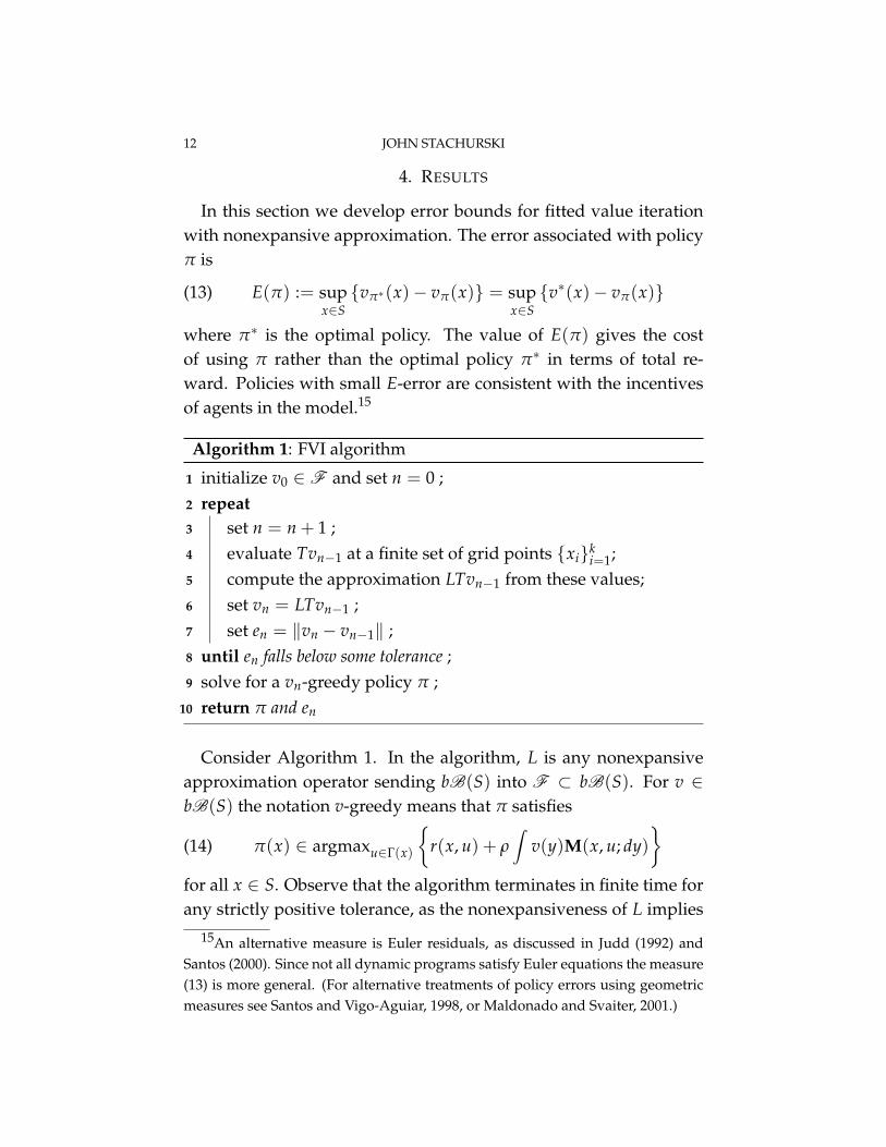
4. RESULTS

In this section we develop error bounds for fitted value iterationwith nonexpansive approximation. The error associated with policyπ is

(13) E(π) := supx∈S

{vπ∗(x)− vπ(x)} = supx∈S

{v∗(x)− vπ(x)}

where π∗ is the optimal policy. The value of E(π) gives the costof using π rather than the optimal policy π∗ in terms of total re-ward. Policies with small E-error are consistent with the incentivesof agents in the model.15

Algorithm 1: FVI algorithm

initialize v0 ∈ F and set n = 0 ;1

repeat2

set n = n + 1 ;3

evaluate Tvn−1 at a finite set of grid points {xi}ki=1;4

compute the approximation LTvn−1 from these values;5

set vn = LTvn−1 ;6

set en = ‖vn − vn−1‖ ;7

until en falls below some tolerance ;8

solve for a vn-greedy policy π ;9

return π and en10

Consider Algorithm 1. In the algorithm, L is any nonexpansiveapproximation operator sending bB(S) into F ⊂ bB(S). For v ∈bB(S) the notation v-greedy means that π satisfies

(14) π(x) ∈ argmaxu∈Γ(x)

{r(x, u) + ρ

∫v(y)M(x, u; dy)

}for all x ∈ S. Observe that the algorithm terminates in finite time forany strictly positive tolerance, as the nonexpansiveness of L implies

15An alternative measure is Euler residuals, as discussed in Judd (1992) andSantos (2000). Since not all dynamic programs satisfy Euler equations the measure(13) is more general. (For alternative treatments of policy errors using geometricmeasures see Santos and Vigo-Aguiar, 1998, or Maldonado and Svaiter, 2001.)

NONEXPANSIVE APPROXIMATION 13

that T := LT is a contraction mapping of modulus ρ, and hence en ≤ρn‖v1 − v0‖ → 0.

Below we adopt the convention that N always denotes the numberof iterations after which the FVI algorithm terminates. It follows thatthe policy π returned by the algorithm is vN-greedy.16

Combining ideas found in Puterman (1994), Judd and Solnick (1994),Gordon (1995), Rust (1996) and Santos and Vigo-Aguiar (1998), onecan establish the following result:

Theorem 4.1. If the FVI algorithm terminates after N iterations, then forevery x ∈ S we have

v∗(x)− vπ(x) ≤ 21− ρ

× (ρeN + ‖LTvN − TvN‖)

The two sources of error in this bound are eN, the deviation of vN

from vN−1 under the supremum norm, and ‖LTvN − TvN‖, whichmeasures the ability of L to approximate the function TvN. The latteris not directly observable, and requires further analysis to bound.Below we give some indications of how this can be done.

The following remarks highlight some key points of the theorem.

Remark 4.1. The bound in Theorem 4.1 should be compared to thebound v∗(x)− vπ(x) ≤ 2ρeN/(1− ρ) given by Puterman (1994, The-orem 6.3.1) for the finite state case, where no approximation is usedand value iteration can be carried out exactly. In the present case, ifthere is no approximation error (i.e., if LTvN = TvN), then the boundin Theorem 4.1 reduces to Puterman’s bound. This suggests that ourbound is relatively tight.

Remark 4.2. It may seem that the error en in the FVI algorithm willbe difficult to evaluate accurately. However, both vn and vn−1 lie in

16In general lines 9 and 10 of the algorithm cannot be implemented exactly.Hence it may be preferable to return the approximate value function vN and eval-uate optimal actions by solving the maximization in (14) as required. In practice,however, computing a good approximation to π by evaluating the right hand sideof (14) at many points in S takes very little computational effort relative to the FVIalgorithm itself, as only one function (i.e., π itself) need be approximated.

14 JOHN STACHURSKI

the simple parametric class F . As a result, evaluation of the error istypically straightforward.

Now we turn to the second theorem of the paper. Suppose forsome reason that the term ‖LTvN − TvN‖ in Theorem 4.1 is difficultto evaluate or bound efficiently. In that case it may be easier to assessthe approximation error ‖Lv∗ − v∗‖. The next result gives a boundusing ‖Lv∗ − v∗‖ instead of ‖LTvN − TvN‖, albeit at the cost of alarger constant term:

Theorem 4.2. If the FVI algorithm terminates after N iterations, then forevery x ∈ S we have

v∗(x)− vπ(x) ≤ 2(1− ρ)2 × (ρeN + ‖Lv∗ − v∗‖)

The proofs of Theorems 4.1 and 4.2 are given in Section 6.

5. REPEATED PARTIAL DISCRETIZATION

Let us consider the FVI algorithm in more detail for the case whereL uses piecewise constant approximation (see Section 3). For reasonsthat become clear below, we refer to this case as repeated partial dis-cretization (RPD). The following RPD algorithm is closely related tostandard discretization, where a continuous state model is replacedby a similar model evolving on a finite grid. At the same time, RPDpossesses several important advantages. One is that, since the ap-proximation operator is nonexpansive, the error bounds developedabove all apply. We show how, in many cases, bounds are easilyderived from a term automatically generated by the FVI algorithm.

A second advantage is that the reward function r and the law ofmotion are never themselves discretized—and nor need they be, asthese are primitives which presumably can be implemented with-out discretization. Thus, RPD does not discard the information con-tained in the values of these functions between the grid points.

Finally, in RPD it is possible to adjust the location and size of thegrid at each iteration. A number of algorithms use variable gridsfor discretized dynamic programming, which allows one to placerelatively many grid points near the areas of greatest curvature (i.e.,

NONEXPANSIVE APPROXIMATION 15

the areas where approximation is most difficult) at each iteration. Wedo not discuss variable grid methods further in this paper.

In what follows we discuss RPD in some detail and give directerror bounds. The method is then applied to a model of stochasticspeculative prices due to Samuelson (1971).

To begin, let S be a subset of Rd with the usual partial order.17

Suppose that S can be written as the union of finitely many disjointrectangles {Ji}k

i=1, where

Ji := [xi, yi) := [x1i , y1

i )× · · · × [xdi , yd

i )

Let C be the set of functions from S to R which are constant oneach Ji. For w ∈ bB(S), define the operator L : bB(S) → C byLw(x) = w(xi) when x ∈ Ji. Below we use the shorthand notationstep[a1, . . . , ak] to mean the piecewise constant function on S givenby the vector (a1, . . . , ak), in the sense that step[a1, . . . , ak] = ai on Ji.In this notation, Lw = step[w(x1), . . . , w(xk)].

5.1. The RPD Algorithm. Consider Algorithm 2, which is a special-ized version of the FVI algorithm corresponding to piecewise con-stant approximation.18 In many situations Algorithm 2 (henceforth,the RPD algorithm) lends itself to simple implementation and yieldsan error bound which is completely specified by observables. Thedetails are in Proposition 5.1.

Proposition 5.1. Let π, R and eN be as returned by the RPD algorithm,which is assumed to terminate after N iterations. If T preserves monotonic-ity, then

v∗(x)− vπ(x) ≤ 21− ρ

× (ρeN + R) (x ∈ S)

whenever the initial condition v0 is monotone increasing.19

17Let x = (xj)dj=1 and y = (yj)d

j=1. Say that x ≤ y if xj ≤ yj for all j.18One apparent difference is that the FVI algorithm defines en as ‖vn − vn−1‖,

while Algorithm 2 defines en = max1≤i≤k |vn(xi)− vn−1(xi)|. But since vj ∈ C forall j it should be clear that these two definitions are equivalent.

19Preservation of monotonicity means that Tw is increasing whenever w ∈bB(S) is increasing.

16 JOHN STACHURSKI

Algorithm 2: RPD algorithm

initialize v0 ∈ C and set n = 0 ;1

repeat2

set n = n + 1 ;3

for i in 1 to k do evaluate Tvn−1(xi) ;4

set LTvn−1 = step[Tvn−1(x1), . . . , Tvn−1(xk)] ;5

set vn = LTvn−1 ;6

set en = max1≤i≤k |vn(xi)− vn−1(xi)| ;7

until en falls below some tolerance ;8

solve for a vn-greedy policy π ;9

set R = max1≤i≤k |Tvn(yi)− Tvn(xi)|;10

return π, R and en11

Remark 5.1. The condition that T preserves monotonicity holds inmany applications. For example, suppose as in (3) that the law ofmotion is given by Xt+1 = F(Xt, Ut, Wt+1), where Wt

IID∼ G(dz). Ifx 7→ F(x, u, z) is increasing for all fixed u and z, and, moreover, x 7→r(x, u) is increasing for all u, then T preserves monotonicity. Thesekinds of results are well-known and further details are omitted.

Remark 5.2. In the RPD algorithm, note that evaluation of R needsno further optimization, as π and vN are available, π is vN-greedy,and

TvN(x) = r(x, π(x)) + ρ∫

vN(y)M(x, π(x); dy) (x ∈ S)

5.2. Application. To further illustrate the ideas, we now apply theRPD algorithm to Samuelson’s (1971) theory of price equilibriumin a commodity market with speculative investment.20 The modelhas recently been the basis of active empirical study of commod-ity prices. We follow Chambers and Bailey (1996) and Deaton andLaroque (1996) in considering a commodity price model with corre-lated supply shocks.

20Code for the following is available on request from the author.

NONEXPANSIVE APPROXIMATION 17

12

3

5

10

1

2

3

policy surface

s

h

FIGURE 1. Optimal investment policy.

Briefly, the model describes intertemporal equilibrium in a singlecommodity market with consumption demand ct determined by in-verse demand function P (pt = P(ct)), and speculative demand qt.Supply st consists of the “harvest” ht plus λqt−1, where λ < 1 is a“shrinkage” parameter and qt−1 is carryover from the last period.The harvest process (ht)∞

t=0 is correlated. We assume in particularthat

ht+1 = θht + (1− θ)Wt+1

where (Wt)∞t=1 is an independent shock process with identical cumu-

lative distribution function G, and θ ∈ (0, 1) is a parameter.Equilibrium prices are determined by arbitrage conditions. Samuel-

son (1971) famously demonstrated that these restrictions correspondto the first order conditions of a dynamic programming problemwith discount factor ρ := (1 + r)−1 and period utility function U(c) =∫ c

0 P(x)dx. The program in question is max E[∑∞

t=0 ρtU(ct)]

subject

18 JOHN STACHURSKI

to restrictions

ct + qt = st, st+1 = λqt + ht+1, s0, h0 given

In the framework of Section 2, the control is q and two-dimensionalstate is x = (s, h). The law of motion is

(s, h, q, z) 7→(

s′

h′

)=

(λq + θh + (1− θ)z

θh + (1− θ)z

)

where a prime denotes next period’s value. If (Wt)∞t=0 takes values

in [z, z], then the same is true of (ht)∞t=0. The state space can be set as

S := [z, z/(1− λ)]× [z, z]

and the feasible correspondence as Γ(s, h) = [0, s]. In particular,(s, h) ∈ S and q ∈ Γ(s, h) implies (s′, h′) ∈ S with probability one.The reward function is U(s− q).21

We set U(c) = cα, and let W = a + bV, where V is beta(5, 5). Theparameters are set to ρ = 0.9, λ = 0.7, θ = 0.3, α = 0.2, a = 1and b = 2. As a result, z = 1 and z = 3. The RPD algorithm wasinitialized with v(s, h) = U(sk) on Jkj.

To study the RPD algorithm, the policy function and the errorbound were computed for different grid sizes after N = 40 itera-tions. Figure 1 gives the approximate optimal policy when the gridsize is 960. Table 1 shows the error bound

21− ρ

× (ρeN + R)

from Proposition 5.1 for different grid sizes (column 2). To put theerrors in context, we used this upper bound on the absolute errorto compute a lower bound on the fraction of total value v∗(x) ob-tained by the approximate optimal policy. (The method is outlinedin the appendix.) The results are shown in column 3. The boundsguarantee that the approximate optimal policy obtains over 95% ofavailable value for a grid size of 1800 and 40 iterations.

21The graph gr Γ is all (s, h, q) with (s, h) ∈ S and 0 ≤ q ≤ s.

NONEXPANSIVE APPROXIMATION 19

grid size error bound value obtained

500 0.765 ≥ 93.1%960 0.623 ≥ 94.4%

1800 0.479 ≥ 95.6%5000 0.451 ≥ 95.9%

TABLE 1. Error bounds by grid size, 40 iterations

6. PROOFS

Let us now address the proof of Theorem 4.1. Since the initialcondition x will vary according to the problem, we construct a boundon the deviation v∗(x) − vπ(x) which is uniform over x ∈ S. Inpractice, this is done by bounding the sup-norm error ‖v∗ − vπ‖.Using the triangle inequality, the sup-norm error is broken down as

(15) ‖v∗ − vπ‖ ≤ ‖v∗ − vN‖+ ‖vN − vπ‖

where vN ∈ bB(S) and N are as in Theorem 4.1. First we bound thefirst term on the right hand side of (15):

Claim 6.1. We have (1− ρ)‖v∗ − vN‖ ≤ ρeN + ‖LTvN − TvN‖.

Proof. By the triangle inequality and the contraction property of T,

‖v∗ − vN‖ ≤ ‖v∗ − TvN‖+ ‖TvN − vN‖≤ ρ‖v∗ − vN‖+ ‖TvN − vN‖

(16) ∴ (1− ρ)‖v∗ − vN‖ ≤ ‖TvN − vN‖

Moreover,

‖TvN − vN‖ ≤ ‖TvN − vN+1‖+ ‖vN+1 − vN‖≤ ‖vN+1 − TvN‖+ ρ‖vN − vN−1‖= ‖LTvN − TvN‖+ ρeN

Putting this together with (16) gives the bound in Claim 6.1. �

Next consider the second term on the right hand side of (15).

20 JOHN STACHURSKI

Claim 6.2. We have (1− ρ)‖vN − vπ‖ ≤ ρeN + ‖LTvN − TvN‖.

Proof. By the triangle inequality,

(17) ‖vN − vπ‖ ≤ ‖vN − TvN‖+ ‖TvN − vπ‖

Consider the second term in the right hand side of (17). From thedefinition of the Bellman operator T we have

TvN(x) = maxu∈Γ(x)

{r(x, u) + ρ

∫vN(y)M(x, u; dy)

}One the other hand, by the definition of the operator Tπ,

TπvN(x) = r(x, π(x)) + ρ∫

vN(y)M(x, π(x); dy)

Since π is vN-greedy, TvN and TπvN are equal. Moreover, we knowthat Tπ is a contraction of modulus ρ, and vπ is the unique fixedpoint. Hence

‖TvN − vπ‖ = ‖TπvN − Tπvπ‖ ≤ ρ‖vN − vπ‖

Substituting this into (17) we get

‖vN − vπ‖ ≤ ‖vN − TvN‖+ ρ‖vN − vπ‖

(18) ∴ (1− ρ)‖vN − vπ‖ ≤ ‖vN − TvN‖

Finally, we have already shown in the proof of Claim 6.1 that

‖TvN − vN‖ ≤ ‖LTvN − TvN‖+ ρeN

Substituting this into (18) gives the bound that we are seeking. �

Proof of Theorem 4.1. From (15) and Claims 6.1 and 6.2 we get

(1− ρ)‖v∗ − vπ‖ ≤ 2(ρeN + ‖LTvN − TvN‖)

The bound in Theorem 4.1 follows immediately. �

Next we turn to the proof of Theorem 4.2. The proof is based onthe following two estimates:

Claim 6.3. If π is vN-greedy, then we have

(19) (1− ρ)‖v∗ − vπ‖ ≤ 2‖vN − v∗‖

NONEXPANSIVE APPROXIMATION 21

Proof. We have

(20) ‖v∗ − vπ‖ ≤ ‖v∗ − vN‖+ ‖vN − vπ‖

On the other hand,

(21) ‖vN − vπ‖ ≤ ‖vN − TvN‖+ ‖TvN − vπ‖

Consider the first term on the right hand side of (21). Observe thatfor any w ∈ bB(S) we have

‖w− Tw‖ ≤ ‖w− v∗‖+ ‖v∗ − Tw‖≤ ‖w− v∗‖+ ρ‖v∗ − w‖ = (1 + ρ)‖w− v∗‖

Substituting in vN for w, we obtain

(22) ‖vN − TvN‖ ≤ (1 + ρ)‖vN − v∗‖

Now consider the second term on the right hand side of (21). Ithas already been observed that for this particular policy π we haveTvN = TπvN, so

‖TvN − vπ‖ = ‖TπvN − vπ‖ = ‖TπvN − Tπvπ‖ ≤ ρ‖vN − vπ‖

Substituting this bound and (22) into (21), we obtain

‖vN − vπ‖ ≤ (1 + ρ)‖vN − v∗‖+ ρ‖vN − vπ‖

∴ ‖vN − vπ‖ ≤1 + ρ

1− ρ‖vN − v∗‖

This inequality and (20) together give

‖v∗ − vπ‖ ≤ ‖v∗ − vN‖+1 + ρ

1− ρ‖vN − v∗‖

Simple algebra now gives (19). �

Claim 6.4. For every n ∈ N we have

(1− ρ)‖v∗ − vn‖ ≤ ‖v∗ − Lv∗‖+ ρ‖vn − vn−1‖

Proof. Let v be the fixed point of T. By the triangle inequality,

(23) ‖v∗ − vn‖ ≤ ‖v∗ − v‖+ ‖v− vn‖

22 JOHN STACHURSKI

Regarding the first term on the right hand side of (23), we have

‖v∗ − v‖ ≤ ‖v∗ − Tv∗‖+ ‖Tv∗ − v‖

= ‖v∗ − Lv∗‖+ ‖Tv∗ − Tv‖ ≤ ‖v∗ − Lv∗‖+ ρ‖v∗ − v‖

(24) ∴ (1− ρ)‖v∗ − v‖ ≤ ‖v∗ − Lv∗‖

Regarding the second term in the sum (23), we have

‖v− vn‖ ≤ ‖v− Tn+1v0‖+ ‖Tn+1v0 − Tnv0‖≤ ρ‖v− vn‖+ ρ‖vn − vn−1‖

(25) ∴ (1− ρ)‖v− vn‖ ≤ ρ‖vn − vn−1‖

Combining (23), (24) and (25) gives the bound we are seeking. �

Proof of Theorem 4.2. Pick any x ∈ S, and suppose that the value iter-ation algorithm terminates after N steps. By Claim 6.3 we have

v∗(x)− vπ(x) ≤ 21− ρ

‖vN − v∗‖

Applying Claim 6.4, this becomes

v∗(x)− vπ(x) ≤ 2(1− ρ)2 (ρ‖vN − vN−1‖+ ‖v∗ − Lv∗‖)

The claim in Theorem 4.2 now follows from the definition of eN. �

Proof of Proposition 5.1. The proof is almost trivial. Since the RPD al-gorithm is a special case of the FVI algorithm, Theorem 4.1 gives

v∗(x)− vπ(x) ≤ 21− ρ

× (ρeN + ‖LTvN − TvN‖) (x ∈ S)

where N is the number of iterations after which the RPD algorithmterminates. Thus we need only show that ‖Lw − w‖ ≤ R, wherew := TvN. In doing so, notice that w is monotone increasing, as theinitial condition v0 has this property, and T preserves monotonic-ity.22

22Clearly L automatically preserves monotonicity, and hence so does T.

NONEXPANSIVE APPROXIMATION 23

So suppose to the contrary that there is an x ∈ S with |Lw(x) −w(x)| > R. Without loss of generality, assume that x ∈ Jm, so that

R < |Lw(x)− w(x)| = |w(xm)− w(x)| = w(x)− w(xm)

where the last step is by monotonicity. On the other hand, we have

w(ym)− w(xm) ≤ max1≤i≤k

|w(yi)− w(xi)| =: R

Putting these two inequalities together gives w(ym) < w(xm), whichcontradicts monotonicity of w. �

Finally we discuss the technique used to obtain the lower boundon the fraction of total value v∗(x) obtained by the approximate op-timal policy π, as shown in column 3 of Table 1. The fraction inquestion is vπ(x)/v∗(x). Regarding this fraction, observe that

v∗(x)− vπ(x)v∗(x)

≤ v∗(x)− vπ(x)v∗(z, z)

≤ v∗(x)− vπ(x)vN(z, z)

≤ 21− ρ

× ρeN + RvN(z, z)

:= β

where the first equation is by monotonicity of v∗ and the second fol-lows from our choice of initial condition. The value β can be com-puted from the second column of Table 1 and the term vN(z, z). Nownote that

vπ(x)v∗(x)

= 1− v∗(x)− vπ(x)v∗(x)

≥ 1− β

REFERENCES

[1] Aruoba, S. B., J. Fernandez-Villaverde and J. F. Rubio-Ramirez (2006): “Com-paring Solution Methods for Dynamic Equilibrium Economies, Journal of Eco-nomic Dynamics and Control, 30 (12), 2477–2508.

[2] M.J. Chambers and R.J. Bailey (1996): “A Theory of Commodity Price Fluctu-ations,” Journal of Political Economy, 104(5), 924–957.

[3] Deaton, A. and G. Laroque (1996): “Comptetitive Storage and CommodityPrice Dynamics,” Journal of Political Economy, 104(5), 896–923.

[4] Drummond, C (1996): “Preventing Overshoot of Splines with Application toreinforcement Learning,” Computer Science Dept. Ottawa TR-96-05.

24 JOHN STACHURSKI

[5] Gordon, G.J. (1995): “Stable Function Approximation in Dynamic Program-ming,” Proceedings of the 12th International Conference on Machine Learn-ing.

[6] Guestrin, C., D. Koller and R. Parr (2001): “Max-Norm Projections for Fac-tored MDPs,” International Joint Conference on Artificial Intelligence, Vol. 1,673–680.

[7] Hernandez-Lerma, O., and J.B. Lasserre (1999): Further Topics in Discrete-TimeMarkov Control Processes, Springer-Verlag, New York.

[8] Judd, K.L. (1992): “Projection Methods for Solving Aggregate Growth Mod-els,” Journal of Economic Theory, 58 (2), 410–452.

[9] Judd, K.L. and A. Solnick (1994): “Numerical Dynamic Programming withShape-Preserving Splines,” unpublished manuscript.

[10] Lyche, T and K. Mørken (2002): Spline Methods, mimeo, University of Oslo.[11] Maldonado, W. L. and B. F. Svaiter (2001): “On the Accuracy of the Estimated

Policy Function using the Bellman Contraction Method,” Economics Bulletin,(3) 15, 1–8.

[12] Munos, R. and A. Moore (1999): “Variable Resolution Discretization in Opti-mal Control,” Machine Learning, 1, 1–24.

[13] Puterman, M. (1994): Markov Decision Processes: Discrete Stochastic DynamicProgramming, John Wiley & Sons, New York.

[14] Rust, J. (1996): “Numerical Dynamic Programming in Economics,” in H. Am-man, D. Kendrick and J. Rust (eds.) Handbook of Computational Economics, El-sevier, North Holland.

[15] Rust, J. (1997): “Using Randomization to Break the Curse of Dimensionality,”Econometrica, 65 (3), 487–516.

[16] Samuelson, P.A. (1971): “Stochastic Speculative Price,” Proceedings of the Na-tional Academy of Science, 68 (2), 335–337.

[17] Santos, M.S. and J. Vigo-Aguiar (1998): “Analysis of a Numerical DynamicProgramming Algorithm Applied to Economic Models,” Econometrica, 66(2),409–426.

[18] Santos, M.S. (2000): “Accuracy of Numerical Solutions Using the Euler Equa-tion Residuals,” Econometrica, 68 (6), 1377–1402.

[19] Stokey, N. L., R. E. Lucas and E. C. Prescott (1989): Recursive Methods in Eco-nomic Dynamics, Harvard University Press, Massachusetts.

[20] Tsitsiklis, J.N. and B. Van Roy (1996): “Feature-Based Methods for Large ScaleDynamic Programming,” Machine Learning, 22, 59–94.

INSTITUTE OF ECONOMIC RESEARCH, KYOTO UNIVERSITY, YOSHIDA-HONMACHI,SAKYO-KU, KYOTO 606-8501, JAPAN

E-mail address: john@kier.kyoto-u.ac.jp