Outline

Construction of gravity and magnetic models Principle of superposition (mentioned on week 1) Anomalies

Reference models Geoid Figure of the Earth Reference ellipsoids

Gravity corrections and anomalies Calibration, Drift, Latitude, Free air, Bouguer, Terrain,

Aeromagnetic data reduction, leveling, and processing

Gravity anomalies The isolation of anomalies (related to unknown local

structure) is achieved through a series of corrections to the observed gravity for the predictable regional effects

According to Blakely (page 137), it is best to view the corrections as superposition of contributions of various factors to the observed gravity (next slide)

Gravity anomaliesObserved gravity = attraction of the reference

ellipsoid (figure of the Earth)

+ effect of the atmosphere (for some ellipsoids)+ effect of the elevation above sea level (free

air)+ effect if the “average” mass above sea level

(Bouguer and terrain)+ time-dependent variations (drift and tidal)+ effect of moving platform (Eötvös)+ effect of masses that would support

topographic loads (isostatic)

+ effect of crust and upper mantle density (“geology”)

If we model and subtract these terms from the data…

…then the remainder is the “anomaly” (for example, “free air” or “Bouguer” gravity)

Geoid and Reference Ellipsoid Geoid is the actual equipotential surface at

(regional) mean sea level Reference ellipsoid is the equipotential

surface in a uniform Earth Much more precisely known from GPS and satellite

gravity data Recent recommendations are to reference all

corrections to the reference ellipsoids and not to the geoid

Hydrostatic rotating Earth The surface of static fluid has a constant potential :

22

polar2 2 23 3

1 1 1, sin

2 2 2

rrU r GM r const GM

R R

22 3

2

polar

1 sin 1r R

r GM

2 3

polar 2polar2 3

2

1 sin2

1 sin

r Rr r

GMRGM

Therefore:

Gravity potentialCentrifugal potential

Conventionally, the equatorial radius is used for referencing:

21 coser r f

Gravity flattening Because of increased radius and rotation, gravity

is reduced at the equator:

21 coseg g

b is called the “gravity flattening”:

p e

e

g g

g

Reference Ellipsoids International Gravity Formula

Established in 1930; IGF30 Updated: IGF67

World Geodetic System (last revision 1984; WGS84) Established by U.S. Dept of Defense Used by GPS So the gravity field is measured above the atmosphere The difference from IGF30 can be ~100 m

A number of other older ellipsoids used in cartography

Also note the International Geomagnetic Reference Field: IGRF-11

Gravity flattening and the shape of the Earth Exercise: from the expressions for the Earth’s

figure and gravity flattening, show that the radius can be estimated from measured gravity as:

251 cos

2ee

gr r m

g

Multi-year drift of our gravity meter During field schools, the G267 gravimeter usually drifts by 0.1-0.2 mGal/day

Bullard B correction Necessary at high elevations (airborne gravity) Added to Bouguer slab gravity (subtracted from Bouguer-

corrected gravity) to account for the sphericity of the Earth

3 7 2 14 3 mGal (with i1.464 10 3.533 10 4.5 10 n meters) B h h hB h

Elevation above reference ellipsoid, h (m)

Bulla

rd B

corr

ect

ion (

mG

al)

Instrument Drift correction During the measurement, the instrument is used at

sites with different gravity gs and also experiences a time-dependent drift d(tobs)

Therefore, the value measured at time tobs at station s is:

obs obss su t g d t For d(tobs), we would usually use some simple

dependence, for example: a polynomial function

0

nk k

kk

d t a t t

where d0 is selected to ensure zero mean: <d(t)> = 0, that is:

00

nk

kk

d t a t d

(*)

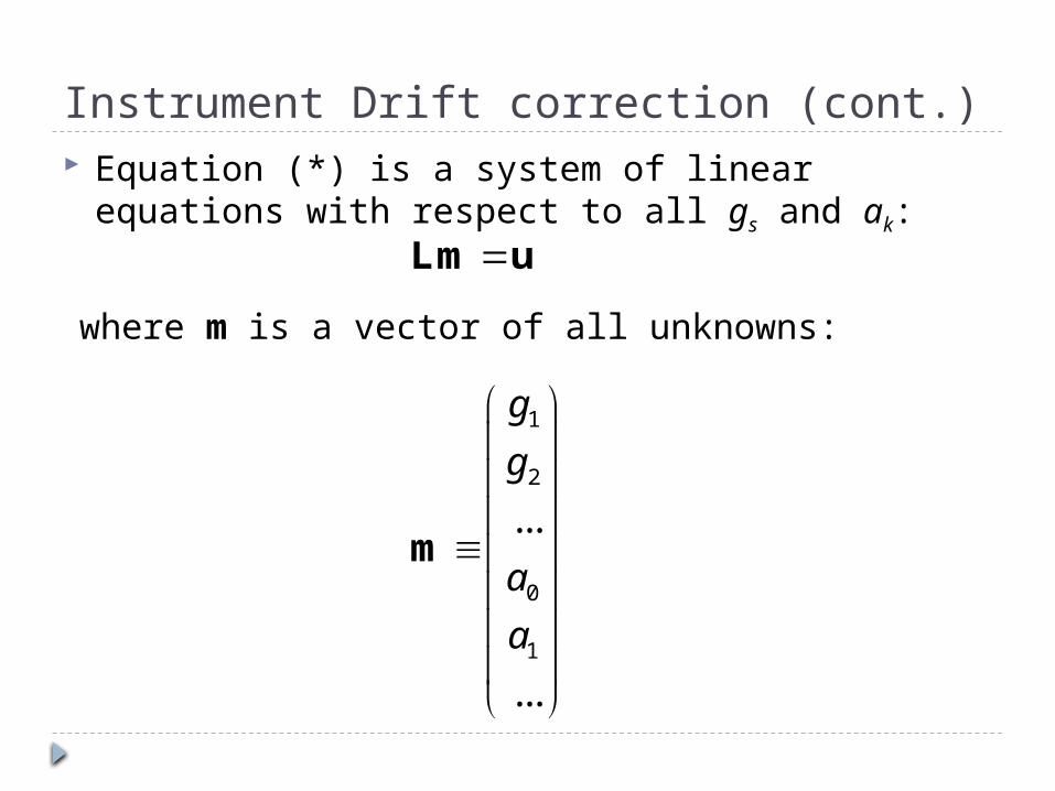
Instrument Drift correction (cont.) Equation (*) is a system of linear equations with

respect to all gs and ak:Lm u

where m is a vector of all unknowns:

1

2

0

1

...

...

g

g

a

a

m

Instrument Drift correction (cont.)

… u is a vector of all observed values:

1 1

1 2

1

...

...

n m

n m

u t

u t

u t

u t

u

Instrument Drift correction (cont.)

… and matrix L looks like this:

21 1

22 2

23 3

24 4

25 5

0 1 ...

0 1 ...

1 0 ...

1 0 ...

1 0 ...

... ... ... ... ...

t t t t

t t t t

t t t t

t t t t

t t t t

L

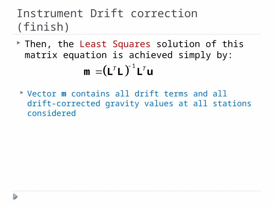
Instrument Drift correction (finish)

1T Tm L L L u

Then, the Least Squares solution of this matrix equation is achieved simply by:

Vector m contains all drift terms and all drift-corrected gravity values at all stations considered