AUTHORS

Guochang Wang � Department of Geologyand Geography, West Virginia University, Morgan-town, West Virginia; Key Laboratory of Tectonicsand Petroleum Resources Ministry of Education,China University of Geosciences (Wuhan), Wuhan,Hubei, People’s Republic of China; present address:College of Earth Science, University of ChineseAcademy of Sciences, No. 19A Yuquan Road,Beijing China 100049; w.guochang@gmail.com

Organic-rich Marcellus Shalelithofacies modeling anddistribution pattern analysis inthe Appalachian BasinGuochang Wang and Timothy R. Carr

Guochang Wang received his Ph.D. in geology(2012) from West Virginia University and is underthe Chinese Government scholarship through theChina University of Geosciences (Wuhan). He iscurrently working on the unconventional gas teamof the University of Chinese Academy of Sciencesin Beijing, China. Recent interests include reservoircharacterization of shale gas and coalbed methanereservoirs, hydraulic fracturing, logging analysis,and seismic interpretation.

Timothy R. Carr � Department of Geologyand Geography, West Virginia University, Mor-gantown, West Virginia and National EnergyTechnology Laboratory, Pittsburgh, Pennsylvania;tim.carr@mail.wvu.edu

Tim Carr is currently the Marshall Miller Professorat West Virginia University. Since graduating with aPh.D. from the University of Wisconsin–Madison,he has worked in various areas of energy geo-sciences. Previously, he was employed at ARCO Oiland Gas, the Kansas Geological Survey, and theUniversity of Kansas. His current interests includeunconventional resources, CO2 use and geologicstorage, quantitative techniques, scientific cyberinfrastructure, and energy policy.

ACKNOWLEDGEMENTS

As part of the National Energy Technology Lab-oratory’s Regional University Alliance (NETL-RUA),a collaborative initiative of the NETL, this technicaleffort was performed under the RES contract DE-FE0004000, and also funded by the National NaturalScience Foundation of China (no. 698796867). Wethank the Energy Corporation of America, ConsolEnergy, EQT Production, and the Petroleum Devel-opment Corporation for providing the data. Math-Works (Matlab), Schlumberger (PETREL), and Geo-

ABSTRACT

The Marcellus Shale is considered to be the largest uncon-ventional shale-gas resource in the United States. Two criticalfactors for unconventional shale reservoirs are the response ofa unit to hydraulic fracture stimulation and gas content. Thefracture attributes reflect the geomechanical properties of therocks, which are partly related to rock mineralogy. The naturalgas content of a shale reservoir rock is strongly linked to or-ganic matter content,measured by total organic carbon (TOC).A mudstone lithofacies is a vertically and laterally continuouszone with similar mineral composition, rock geomechanicalproperties, and TOC content. Core, log, and seismic datawere used to build a three-dimensional (3-D) mudrock litho-facies model from core to wells and, finally, to regional scale.An artificial neural networkwas used for lithofacies prediction.Eight petrophysical parameters derived from conventionallogs were determined as critical inputs. Advanced logs, suchas pulsed neutron spectroscopy, with log-determinedmineralcomposition and TOC data were used to improve and con-firm the quantitative relationship between conventional logsand lithofacies. Sequential indicator simulation performedwell for 3-D modeling of Marcellus Shale lithofacies. The in-terplay of dilution by terrigenous detritus, organic matter pro-ductivity, and organic matter preservation and decompositionaffected the distribution of Marcellus Shale lithofacies distri-bution, which may be attributed to water depth and the dis-tance to shoreline. The trend of normalized average gas pro-duction rate from horizontal wells supported our approachto modeling Marcellus Shale lithofacies. The proposed 3-D

plus Corporation (PETRA) provided access to thesoftware used in this project. We also thank our re-viewers Gary G. Lash, Terrilyn M. Olson, and Mark D.Sonnenfeld for their significant input.The AAPG Editor thanks the following reviewers fortheir work on this paper: Gary G. Lash, Terrilyn M.Olson, and Mark D. Sonnenfeld.

Copyright ©2013. The American Association of Petroleum Geologists. All rights reserved.

Manuscript received July 27, 2012; provisional acceptance December 20, 2012; revised manuscriptreceived March 18, 2013; final acceptance May 14, 2013.DOI:10.1306/05141312135

AAPG Bulletin, v. 97, no. 12 (December 2013), pp. 2173–2205 2173

modeling approach may be helpful for optimiz-ing the design of horizontal well trajectories andhydraulic fracture stimulation strategies.

INTRODUCTION

In the last 10 yr, tremendous progress has beenmade in the exploration and development of un-conventional gas worldwide, especially in NorthAmerica. The application of horizontal drilling andhydraulic fracture stimulation technologies provideseconomic gas flow from extremely low porosity andpermeability reservoirs. However, geologic studiesof lithofacies, as a basic property of reservoirs, aidin optimizing the design of horizontal wells andstimulation strategies in unconventional reservoirs.Lithofacies research historically focused on sand-stone and carbonate reservoirs, including lithofaciesclassification and description from core data andoutcrops (e.g., Bridge et al., 2000; Porta et al., 2002),lithofacies prediction by wireline logs and seismicvolumes (e.g., Berteig et al., 1985; Wong et al.,1995; Chang et al., 2000; Yao and Chopra, 2000;Qi and Carr, 2006; Dubois et al., 2007), litho-facies modeling in two and three dimensions (e.g.,Akatsuka, 2000; Qi et al., 2007), and the relation-ships of lithofacies with reservoir properties (e.g.,Doyle and Sweet, 1995; Akatsuka, 2000). Mud-stone lithofacies research is just at the beginning(Javadpour, 2009; Curtis et al., 2010; Aplin andMacquaker, 2011; Loucks et al., 2012) and pri-marily focused on the classification and descriptionfrom core and outcrop observations (Hickey andHenk, 2007; Loucks and Ruppel; 2007; Singh,2008;Walker-Milani, 2011; Zhou et al., 2012). Todate, there are few studies on the prediction of shalelithofacies based on petrophysical and geophysicaldata (Perez, 2009; Vallejo, 2010; Koesoemadinataet al., 2011; Jonk et al., 2012) and little researchconcerning modeling of mudrock lithofacies.

Generation of a mudrock lithofacies model ordistribution pattern can aid in the recognition oforganic-rich and relatively brittle stratigraphic hori-zons, which are important parameters in maximiz-ing shale-gas production rates (Bowker, 2007;Wang

2174 Organic-Rich Shale Lithofacies Modeling, Appalachian Ba

and Carr, 2012a, b). More organic-rich intervalscontain higher concentrations of natural gas, andbrittle horizons tend to be amenable to fracturestimulation. Indeed, the mineral composition of astratigraphic horizon exerts a strong control on rockgeomechanical properties. Specifically, elevatedconcentrations of quartz and carbonate mineralsimprove the brittleness of mudrock, whereas con-centration of clay minerals increases mudrock duc-tility (Jarvie et al., 2007; Mavko, 2010). Lithofaciesare a product of depositional composition and dia-genesis and can provide a valuable framework forunderstanding the correlation between mechanicalstratigraphy and fracture attributes (e.g., Laubachet al., 2009). Mineralogy can affect porosity andpore structure with an impact on permeability andthe potential ratio of free to absorbed gas in mud-stone reservoirs (Loucks et al., 2012). Our analysisof wireline-log signatures and seismic data per-mits the recognition of sevenmudrock lithofaciesof the Marcellus Shale. The various lithofacies re-flect variations of mineral composition and organicmatter richness. The Marcellus Shale lithofacies,first recognized at the core scale, can be predictedfrom conventional logs using artificial neural net-work (ANN). Petrophysical analysis is used to de-rive input variables for ANN classifiers. The log-predicted lithofacies provides a large number ofconstraint points in building three-dimensional(3-D) lithofacies models. Geostatistical reservoirmodeling is used to reconcile available hard andsoft data in a numerical model, providing an overallunderstanding of reservoirs (Deutsch, 2002). Ourmain objective is to provide a quantitative geo-logic framework for unconventional explorationand development decisions to maximize produc-tivity. We use the Marcellus Shale 3-D lithofaciesmodel to (1) investigate the distribution of eachlithofacies at a basin scale, (2) develop a betterunderstanding of the factors controlling the depo-sition and preservation of organic matter and thedepositional model of marine organic-rich mud-rock, (3) identify organic-rich and brittle units inshale-gas reservoirs at scales from an individualwell to basin, (4) assist in the design of horizontaldrilling trajectories and location of stimulation ac-tivity, and (5) provide input parameters for the

sin

characterization that allows the simulation of gasflow and production in mudrock (e.g., porosity,permeability, and fractures).

For the Marcellus Shale in the AppalachianBasin, we propose methods to better identify thecritical geologic parameters to focus on horizontaldrilling and stimulation strategies. By investigatingthe distribution pattern of black mudstone litho-facies laterally and vertically, we hope to betterunderstand black mudstone deposition at the ba-sin scale.

GEOLOGIC SETTING

The Paleozoic history of the Appalachian Basinconsists of three orogenic events induced by col-lisions between the North American plate (Lau-rentia) and the eastern oceanic crust, convertingthe region from a passive margin during the Or-dovician to a foreland basin and a narrow seaway(U.S. Geological Survey, 2004; Marshak, 2010). Atvarious periods, the basin was the site of restrictedcirculation and accumulation of organic-rich units(e.g., Utica-Point Pleasant and Marcellus). The Aca-dian orogeny, beginning in the Middle Devonian,resulted in subsidence near the Acadianmountainsand uplift on the opposite side caused by the flex-ural deformation (Marshak, 2010). During theMiddle and Late Devonian, the Appalachian fore-land basin was bounded by the developing Acadianmountains on the east and south, the Cincinnatiarch on the west, and the Old Red Sandstone con-tinent to the north, and was connected to the Theicocean by a long and narrow seaway in the south-west, forming a nearly enclosed epicontinental sea(Ettensohn and Barron, 1981a; Gao et al., 2000).Tectonic loading stemming from this event coupledwith eustatic sea level rise terminated shallow-shelfcarbonate deposition during the Early Devonianand led to the accumulation of several organic-richshale units, including the Marcellus Shale.

The Marcellus Shale of the Appalachian Basinis one of the most active and successful shale-gasreservoirs in the world. Annual natural gas pro-duction from theMarcellus in 2012 has grown fromless than 100 mmcf in 2004 to more than 2 tcf.

In addition, the annual production of natural gasliquids while constrained by infrastructure is ap-proximately 2 million bbl. The Marcellus Shalecovers most parts of the basin with an area approx-imately 500,000 km2 (191,000mi2) (Figure 1). Theaverage gross thickness and organic-rich (total or-ganic carbon [TOC], >6.5%) intervals of the Mar-cellus Shale are approximately 80 ft (24 m, rang-ing from 0 to 98 ft [0–30 m]; Figure 1) and 34 ft(10m, ranging from 0 to 177 ft [0–54m]; Figure 1),respectively. The Middle Devonian central Appa-lachian Basin was situated approximately 25°–35°south of the paleoequator (VerStraeten, 2007).The Acadianmountainsmay have blocked easterlytrade winds that carriedmoisture from the easternocean, creating a rain shadow effect on the west-ern side of the mountains (Ettensohn and Barron,1981b; Woodrow and Sevon, 1985). The paleo-climate was believed to have been hot with sea-sonally restricted rainfall and occasional largestorms (Woodrow and Sevon, 1985;Werne et al.,2002). The primary formations deposited dur-ing the Middle Devonian include the OnondagaLimestone, Marcellus Shale, Mahantango Forma-tion, and Tully Limestone, from oldest to youngest(Figure 2). Most of the Middle Devonian organic-rich mudrock is located in the Marcellus Shale,with a few organic-rich units in the MahantangoFormation in New York State (Brett and Baird,1996). The Marcellus Shale is believed to havebeen deposited over a span of 2 m.y. (7–8 m.y. forthewholeHamiltonGroup andTully Limestone) ina relatively deep and anoxicwater (~200m[656 ft])(Brett and Baird, 1996). However, others havesuggested shallow depths for the deposition of theMarcellus and organic-rich shale units in the Ap-palachian Basin (e.g., Smith, 2010).

AVAILABLE DATA

The primary available data consist of limited coredata, abundant wireline logs, two 3-D seismic vol-umes, and Marcellus Shale production data. Eigh-teen wells with core data were accessible and in-clude scanned core pictures, thin sections, and x-raydiffraction (XRD) and geochemical analyses data

Wang and Carr 2175

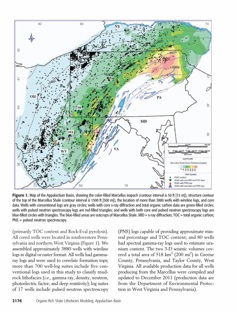
Figure 1. Map of the Appalachian Basin, showing the color-filled Marcellus isopach (contour interval is 50 ft [15 m]), structure contourof the top of the Marcellus Shale (contour interval is 1500 ft [500 m]), the location of more than 3880 wells with wireline logs, and coredata. Wells with conventional logs are gray circles; wells with core x-ray diffraction and total organic carbon data are green-filled circles;wells with pulsed neutron spectroscopy logs are red-filled triangles; and wells with both core and pulsed neutron spectroscopy logs areblue-filled circles with triangles. The blue-filled areas are outcrops of Marcellus Shale. XRD = x-ray diffraction; TOC = total organic carbon;PNS = pulsed neutron spectroscopy.

(primarily TOC content and Rock-Eval pyrolysis).All cored wells were located in southwestern Penn-sylvania and northern West Virginia (Figure 1). Weassembled approximately 3880 wells with wirelinelogs in digital or raster format: All wells had gamma-ray logs and were used to correlate formation tops;more than 700 well-log suites include five con-ventional logs used in this study to classify mud-rock lithofacies (i.e., gamma ray, density, neutron,photoelectric factor, and deep resistivity); log suitesof 17 wells include pulsed neutron spectroscopy

2176 Organic-Rich Shale Lithofacies Modeling, Appalachian Ba

(PNS) logs capable of providing approximate min-eral percentage and TOC content; and 80 wellshad spectral gamma-ray logs used to estimate ura-nium content. The two 3-D seismic volumes cov-ered a total area of 518 km2 (200 mi2) in GreeneCounty, Pennsylvania, and Taylor County, WestVirginia. All available production data for all wellsproducing from the Marcellus were compiled andupdated to December 2011 (production data arefrom the Department of Environmental Protec-tion in West Virginia and Pennsylvania).

sin

Figure 2. Generalized representation ofthe Middle Devonian lithostratigraphy inthe Appalachian Basin, showing the vari-ation from east to west into the basin ofTully Limestone, Hamilton Group, andOnondaga Limestone. Sys = system.

METHODOLOGY

The integrated method of mudrock lithofaciesmodeling used in this study includes (1) classify-ing lithofacies based on limited available core data,(2) classifying lithofacies with wireline logs at thewell-scale, and (3) building a 3-D lithofacies modelor two-dimensional map of lithofacies distribu-tion. Core XRD and TOC data from 18wells wereevaluated statistically and used to define MarcellusShale lithofacies in terms of two key factors forshale-gas reservoirs: mineralogy and organicmatterrichness (Wang and Carr, 2012a, b, c). Three pri-mary criteria derived from XRD and TOC datawere used to classify black mudrock lithofaciesquantitatively: clay percentage, ratio of quartz tocarbonate (RQC), and TOC content. The Marcel-lus Shale lithofacies were correlated with wireline-log information (Wang and Carr, 2012a, b, c). ThePNS logs calibrated to core data provide mineralpercentage and TOC content and were used toclassify Marcellus Shale lithofacies following thethree criteria developed from the core. The PNS-

defined mudrock lithofacies calibrated to the XRD-defined lithofacies provide the training data setthat was used to classify lithofacies from conven-tional logs for the prediction of all available wellswith the suite of five selected conventional logs.Artificial neural network was the preferred quan-titative method to build the relationship betweenMarcellus Shale lithofacies defined by core andPNS logs to the suite of conventional logs. A singleANN with seven output nodes (the number ofdefined lithofacies) and amodular ANNwere builtand trained to predictMarcellus Shale lithofacies atthe well scale.

A 3-D structural model of major units wasconstructed to cover the Appalachian Basin andthe Middle Devonian formations (Figures 1, 2) toprovide a framework for the 3-D lithofacies model.Unit boundaries from the available log database of3880 wells were used to interpret the correspond-ing structure maps in the Appalachian Basin. Withregard to the tectonic pattern in the AppalachianBasin, regional faults were identified and inter-preted through recognized fault points in wireline

Wang and Carr 2177

Figure 3. The workflow used in thisstudy showing the methodology to inte-grate core data, pulsed neutron spectros-copy logs, conventional logs, and seismicdata and regional geologic knowledge toconstruct a three-dimensional (3-D) mud-rock lithofacies model for the MarcellusShale of the Appalachian Basin. GR =gamma-ray log; PE = photoelectric factorlog; XRD = x-ray diffraction; TOC = totalorganic carbon; PNS = pulsed neutronspectroscopy; RHOB = density log.

logs, abnormal changes in thickness from prelimi-narily interpreted structure maps, and the 3-D seis-mic volumes and attributes. The interpreted unitboundaries, faults, and resulting structure mapswere incorporated into a 3-D structural model withfault model, horizons (formation structure), andzones. The log-predicted Marcellus Shale litho-facies were upscaled and assigned to the cells thatwere penetrated by the wells. A geostatistical anal-ysis was conducted to investigate and summarizethe lateral lithofacies distribution pattern and ge-ometry that were described by variograms for eachMarcellus Shale lithofacies (Qi et al., 2007). De-terministic methods (e.g., kriging) and stochasticmethods (e.g., sequence indicator simulation, trun-cated Gaussian simulation (TGS), multiple-pointstatistics, and the object-basedmethod)wereused toconstruct the 3-D lithofacies models (Falivene et al.,2006; Schlumberger, 2011). Cross sections, surfacemaps, and isopach maps of each lithofacies wereused to observe and visualize the lateral and verticalspatial distributions of Marcellus Shale lithofacies.Production data of Marcellus wells in the Appala-chian Basin were overlain on lithofacies maps toevaluate regional production rate trends. A detailedworkflow integrating core data, PNS logs, con-ventional logs, seismic data, and regional geologic

2178 Organic-Rich Shale Lithofacies Modeling, Appalachian Ba

knowledge was constructed to generate a blackmudstone lithofacies 3-D model (Figure 3).

MARCELLUS SHALE LITHOFACIES

The original definition of lithofacies is the sum ofall the lithologic features in sedimentary rocks, in-cluding texture, color, stratification, structure, com-ponents, and grain-size distribution (Teichert, 1958).Lithofacies (or facies) in sandstone and carbonatesystems have been important in our understand-ing of depositional environments, hydrodynamicconditions, and reservoir properties. For example,the rock texture, stratification, and grain-size distri-bution can differentiate channel sands from flood-plain siltstone, which is significant because of thedistinct differences in depositional porosity andpermeability. In addition, the depositional envi-ronment assists geologists and reservoir engineersin understanding and predicting the heterogeneityand connectivity of reservoirs, which can seriouslyaffect hydrocarbon productivity in the conventionalreservoirs. However, shale-gas and oil-shale mud-rock reservoirs show variation of porosity, perme-ability, and connectivity at much different scalesthan conventional reservoirs. At the wellbore to

sin

Figure 4. (A) A ternary plot showing the mineral composition as a percentage of three major components (i.e., quartz plus feldspar, calciteplus dolomite, and illite plus chlorate) and Rock-Eval total organic carbon (TOC). The boundaries between Marcellus Shale lithofacies areindicated by lines based on clay percentage (green dashed line), the ratio of quartz to carbonate (two blue long dashed lines), and the TOCcontent (filled color of circles). Yellow area = quartz rich; gray area = clay rich; blue area = carbonate rich; pink area = mixture of quartz andcarbonate. (B) Crossplot showing the relationship of higher quartz concentration with higher TOC content. The purple dashed line stands for thetrend of the relationship between TOC and feldspar.

regional scales, the critical heterogeneity in un-conventional mudrock reservoirs is variation inmineral composition and organic content instead ofporosity, permeability, and water saturation (Boyceand Carr, 2010; Wang and Carr, 2012a, b, c). Ourapproach entails the integration and calibrationof widely available conventional well logs withcore and PNS logs to define and classify mudrocklithofacies by mineral composition and organicmatter richness. This approach is important to(1) recognize organic-rich and brittle mudrockfacies; (2) access the large available database ofwell logs to understand the depositional environ-ments and hydrodynamic conditions of mudrockat a regional scale; (3) replace the small variationof rock texture, stratification, grain size, and colorby mineral composition and organic matter rich-ness for lithofacies classification; and (4) avoid theuse of traditional lithofacies parameters such as rocktexture, stratification, structure, and color, which arenot easily recognized with conventional wirelinelogs and seismic data. To keep subsurface litho-facies models meaningful, predictable, and map-pable, core and outcrop, although important, areinsufficient (Ruppel et al., 2012), and subsurface

geologists and engineers have to incorporate wire-line logs and seismic data. We propose a methodspecific to the Marcellus Shale concerning the def-inition and classification of lithofacies that mayhave broader application to other unconventionalmudrock reservoirs.

Based on XRD analyses from 195 samples in18 wells (Figures 1, 4A), the most abundant min-erals in the Marcellus Shale are quartz and illite,averaging 35% and 25% by volume, respectively.Variable volumes of chlorite, pyrite, calcite, dolo-mite, and plagioclase are next in abundance, fol-lowed by K-feldspar, kaolinite, mixed-layer illite-smectite, and apatite. Based on cuts of the samesamples run for XRD, the average TOC contentis greater than 5% by weight, ranging up to 20%.The variable mineral composition of the MarcellusShale leads to differences in geomechanical prop-erties that should be considered in the placementand design of hydraulic fracture stimulations. Wehave categorized the primary minerals into threegroups, which are readily displayed on a ternaryplot (Figures 4A, 5): quartz (quartz, feldspar), car-bonate (calcite, dolomite), and clay (all clay min-erals). Most Marcellus samples contain less than

Wang and Carr 2179

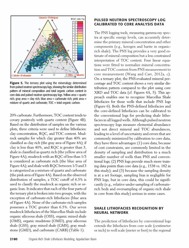
Figure 5. The ternary plot using the mineralogy determinedfrompulsed neutron spectroscopy logs, showing the similar distributionpattern of mineral composition and total organic carbon content incore data and pulsed neutron spectroscopy logs. Yellow area = quartzrich; gray area = clay rich; blue area = carbonate rich; pink area =mixture of quartz and carbonate; TOC = total organic carbon.

20% carbonate. Furthermore, TOC content tends tocovary positively with quartz content (Figure 4B).Based on the distribution of samples on the variousplots, three criteria were used to define lithofacies:clay concentration, RQC, and TOC content. Mud-rock samples for which clay greater than 40% areclassified as clay rich (the gray area of Figure 4A); ifclay is less than 40%, and RQC is greater than 3,shale is classified as quartz rich (the yellow area ofFigure 4A); mudrock with an RQC of less than 1/3is considered as carbonate rich (the blue area ofFigure 4A); and shalewithRQCbetween 1/3 and 3is categorized as a mixture of quartz and carbonate(the pink area of Figure 4A). Based on the observeddistribution of samples, a TOC cutoff of 6.5% isused to classify the mudrock as organic rich or or-ganic lean. It indicates that each of the four parts ofthe ternary plot is broken into two groups, with theexception of carbonate-rich lithofacies (blue areaof Figure 4A). None of the carbonate-rich samplespossesses a TOC greater than 6.5%. Our sevenmudrock lithofacies of the Marcellus Shale includeorganic siliceous shale (OSS), organic mixed shale(OMS), organic mudstone (OMD), gray siliceousshale (GSS), gray mixed shale (GMS), gray mud-stone (GMD), and carbonate (CARB) (Table 1).

2180 Organic-Rich Shale Lithofacies Modeling, Appalachian Ba

PULSED NEUTRON SPECTROSCOPY LOGCALIBRATED TO CORE ANALYSIS DATA

The PNS logging tools, measuring gamma-ray spec-tra at specific energy levels, can accurately deter-mine the primary mineral concentration and othercomponents (e.g., kerogen and barite in organic-rich shale). The PNS log provides a very good es-timate of mineral composition but a less constrainedinterpretation of TOC content. Four linear equa-tions were fitted to normalize mineral concentra-tion and TOC content from PNSmeasurement tocore measurement (Wang and Carr, 2012a, c).On a ternary plot, the PNS-evaluated mineral per-centage and TOC content shows a very similar dis-tribution pattern compared to the plot using coreXRD and TOC data (cf. Figures 4A, 5). This ap-proach enables one to recognize Marcellus Shalelithofacies for those wells that include PNS logs(Figure 6). Both the PNS-defined lithofacies andthe core-defined lithofacies can be calibrated tothe conventional logs for predicting shale litho-facies in all loggedwells. Although pulsed neutronspectroscopy logs measure elemental abundanceand not direct mineral and TOC abundances,leading to a level of uncertainty and errors that arecommonly minimized by calibration to core data,they have three advantages: (1) core data, becauseof cost constraints, are commonly limited in thedensity of sampling and distribution to a muchsmaller number of wells than PNS and conven-tional logs; (2) PNS logs provide much more train-ing data points than core data (e.g., 1538 vs. 182 inthis study); and (3) because the sampling densityis at a set footage, sampling bias is negligible forPNS logs, but in core data, this could be signifi-cantly (e.g., relative under sampling of carbonate-rich beds and oversampling of organic-rich shalein core from this study) serious in some cases.

SHALE LITHOFACIES RECOGNITION BYNEURAL NETWORK

The prediction of lithofacies by conventional logsextends the lithofacies from core scale (centimeteror inch) to well scale (meter or foot) to the regional

sin

Table 1. Summary of the Mineralogy Features and Log Responses of the Seven Lithofacies Defined from Core and Advanced Logs in the Marcellus Shale of the Appalachian Basin*

Wang

andCarr

2181

Figure 6. An example showing logs, modeled mineralogy, and pulsed neutron spectroscopy (PNS) logs that defined Marcellus Shalelithofacies in well 11 (well location shown in Figure 1).OSS = organic siliceous shale; OMS = organic mixed shale; OMD = organicmudstone; GSS = gray siliceous shale; GMS = gray mixed shale; GMD = gray mudstone; CARB = carbonate interval; TOC = total organiccarbon; GR = gamma ray; HCAL = caliper.

scale (kilometer or mile), making a shale lithofaciesmappable. High precision of lithofacies predictionforms the foundation for building a reliable litho-facies model at the scale of interest. It is a chal-lenging and complex task to calibrate conventionallogs to core or core-defined lithofacies. Artificialneural network, onemeans of dealingwith complexnonlinear problems, has been successfully appliedto lithofacies prediction in sandstone and carbonatereservoirs (Chang et al., 2000; Qi and Carr, 2006).Artificial neural network is very flexible in the de-sign of learning algorithm, determining network ar-chitecture, selecting sensitive input variables, andadapting codes for special issues (Wang and Carr,2012b, c).

Two kinds of ANN classifiers were developedto predict lithofacies: a single ANN classifier with

2182 Organic-Rich Shale Lithofacies Modeling, Appalachian Ba

seven output nodes and a modular ANN classifierconsisting of 21 binary ANN classifiers. Both thesingle ANN classifier and the modular ANN clas-sifier have their own strength and weakness. Thesingle ANN classifier is more effective when theamount of training samples is small; on the con-trary, the modular ANN classifier, which decom-poses the multiclass classification problem into sev-eral binary classification problems, is more powerfulwhen there are many training samples. Thus, thesingle ANN classifier with two hidden layers wasused to train the core data set, whereas themodularANN classifier was trained by the PNS-log data set.Both ANN classifiers were used to predict litho-facies in wells accompanied by conventional logs,thereby providing an opportunity to verify the qual-ity of lithofacies prediction by two different data

sin

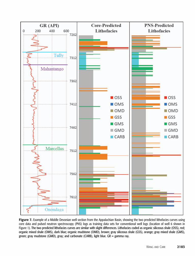
Figure 7. Example of a Middle Devonian well section from the Appalachian Basin, showing the two predicted lithofacies curves usingcore data and pulsed neutron spectroscopy (PNS) logs as training data sets for conventional well logs (location of well 6 shown inFigure 1). The two predicted lithofacies curves are similar with slight differences. Lithofacies coded as organic siliceous shale (OSS), red;organic mixed shale (OMS), dark blue; organic mudstone (OMD), brown; gray siliceous shale (GSS), orange; gray mixed shale (GMS),green; gray mudstone (GMD), gray; and carbonate (CARB), light blue. GR = gamma ray.

Wang and Carr 2183

Figure 8. Two three-dimensional seismic volumes in northern West Virginia (A, B, and C) and southwestern Pennsylvania (D, E, and F),showing the features of reserve faults and strike-slip faults. (A) Time slice of amplitude at approximately 1200 s (two-way traveltime) indicatesseveral strike-slip faults. (B) Cross section aa′ shows a reverse fault dipping to the northwest. (C) Cross section bb′ illustrates two reverse faultsdipping to the southeast. (D) Cross section cc′ in southwestern Pennsylvania shows two reverse faults dipping to the northwest and one reversefault dipping to the southeast. (E) The variation attribute clearly displays major reverse faults. (F) The local azimuth attribute shows largeamounts of small-scale linear features in a direction of northwest–southeast, which were considered as the evidence of strike-slip fault ornorth-south compression stress (unit, degree). In the three cross sections, the light blue line indicates the top of the Tully Limestone, and theblue line, the top of the Onondaga Limestone. The vertical scale on seismic sections is in milliseconds of two-way traveltime.

sets. Therefore, we produced two predicted litho-facies curves using conventional well logs in eachwell (Figure 7). Although a variation exists betweenthe core-derived and the log-derived predicted fa-cies, these are attributed primarily to samplingdifferences; both lithofacies curves were upscaledand extrapolated to build the lithofacies model.

THREE-DIMENSIONAL STRUCTURALAND STRATIGRAPHIC MODEL OFTHE MIDDLE DEVONIAN

To constrain and improve the areal lithofacies mod-eling, we mapped stratigraphic tops and major faultsacross the Appalachian Basin. Several reverse (orthrust) faults and the related strike-slip faults have

2184 Organic-Rich Shale Lithofacies Modeling, Appalachian Ba

been recognized and related to tectonic compres-sional deformation during theAlleghenian orogenyandMesozoic rifting (U.S. Geological Survey, 2004).We interpret additional faults based on (1) faultplanes recognized in well logs, (2) abrupt changesin structure contours, and (3) lateral variation ofseismic signals (Figure 8). Reverse faults were iden-tified through formation repeats observed in welllogs (Figure 9A) or an abrupt thickening of unitsobserved inwell logs and isopachmaps (Figures 9B,C). The structure contour maps constructed fromformation tops highlight abrupt changes of iso-pach in map view (Figure 10). The high density ofwells with log data reduced the uncertainty of faultlocation and strike, although the determination ofdip remained difficult. Even covering small areascompared to the whole Appalachian Basin, the two

sin

Figure 9.Well-log cross sections flatted on the Marcellus Shale, showing the formation repeated in AA′ and formation abrupt thickeningin BB′ and CC′. The purple lines indicated the location of interpreted fault planes. The location of the fault point in section AA′ is welldefined because of the repeated section of the upper Marcellus (Oatka Creek Member). The formation tops downward are Harrell Shale,Tully Limestone, Marcellus Shale, Purcell Member, the base of the Purcell Member, Onondaga Limestone, and the base of the OnondagaLimestone. These sections were hung on the top of the Marcellus Shale. GR = gamma ray.

3-D seismic data sets support the recognition ofregional faults from log data and the estimation offault dips (Figure 8). Seismic amplitude, variationattribute, and local azimuth attribute in section andtime slice clearly define the presence of reverse andstrike-slip faults.

A large number of reverse and strike-slip faultswere interpreted from well logs and 3-D seismicdata, and approximately 30 regional faults werebuilt into the 3-D structural model. Faults arevery common in the northeast of the AppalachianBasin, with two boundary faults in Pennsylvaniaand West Virginia. According to the available seis-mic sections (Figure 8), the dip angle is higher forreverse faults dipping to the northwest than those

dipping to the southeast. Thus, for the 3-D struc-tural model, the dip angle was arbitrarily set to 75°to the west or 65° to the east for reverse faults andapproximately 90° for strike-slip faults.

Formation tops for the Tully Limestone, Ma-hantango Formation, Marcellus Shale, Purcell Lime-stone, and Onondaga Limestone were picked in3880 wells. Marcellus tops were used to generate apreliminary structure contour map (Figure 10A).The structure contour of the Marcellus top wasmodified with the faults model to construct a 3-Dsurface that better represented the present struc-ture of theMarcellus Shale and related formations.In areas with sparse well control or absence of seis-mic data, the structure on the Marcellus and related

Wang and Carr 2185

Figure 10. The structure contour built from the Marcellus Shale top, showing many abnormal changes that were used to interpretreverse faults. (A) The structure contour of the Marcellus Shale top without any faults. (B) A closer view of an example of abnormal jumpin structure map with well locations. (C) The interpreted faults and the rebuilt structure contour of the Marcellus Shale top. The red linestands for the faults in C. The pink line is the boundary of the Marcellus Shale for building the three-dimensional geologic model. (D) Across section view (DD′) of the abrupt change in the top of the Marcellus Shale reflected in panels A, B, and C. Contour interval is 1000 ft(300 m). The unit of depth is feet.

units along with fault geometry could not be deter-mined with confidence. In these areas, it is moreeffective to construct the structural model usingisopach maps and the Marcellus topology as a ref-erence surface. The isopach maps were interpretedfrom the picked tops and corrected by removingcontouring artifacts in the areas without well control(Figure 11).

GEOSTATISTICAL ANALYSIS OFMARCELLUS SHALE LITHOFACIES

Tomodel the lithofacies in 3-D grids, it is essentialto extrapolate lithofacies type fromwells to areas of

2186 Organic-Rich Shale Lithofacies Modeling, Appalachian Ba

low well control. Three-dimensional seismic dataprovide information at the spacing of the stackedseismic bins (tens ofmeters) betweenwells with logsand core. We investigated and defined the trendsin the vertical and lateral distribution of litho-facies based on knowledge developed to understandthe geologic setting, depositional environment, se-quence stratigraphy, and geostatistical analysis con-strained by the predicted lithofacies from conven-tional well logs (e.g., Brett and Baird, 1996; Lash,2008; Boyce and Carr, 2010; Lash and Engelder,2011).

The accumulation of organicmatter is controlledby photosynthetic production, rate of organic matterdecomposition in the water column and sediments,

sin

and detrital sediment dilution (Sageman et al.,2003; Carr et al., 2011). The conditions for theaccumulation of organic-rich shales such as theMarcellus are very complex, but sufficient waterdepth and distance to the sediment source influ-ence shale lithofacies distribution (e.g., Suess,1980; Ibach, 1982; Aplin and Macquaker, 2011).The isopach maps of the Onondaga Limestone,Union Springs Member, Purcell Limestone, andOatka Creek Member and the strike of the re-gional reverse faults indicate that the depositionshelf took a shape of a crescent with a major north-northwest component, as indicated by the isopachmaps of the Onondaga Limestone and Tully Lime-stone (Figure 11). As a result, to follow the isopachtrends, we set the major direction of geostatisticalellipse to 40° for the 3-D geologic modeling ofMarcellus Shale lithofacies. In the vertical direc-tion, the proportion of organic siliceous shale de-creases upward with a clear increase of gray mud-stone in the Oatka Creek Member and is attributedto the progradation and fall in relative sea level(Figure 12A) (Lash and Engelder, 2011). In addi-tion to organic-rich facies, the observed verticalvariation of shale lithofacies increases from theUnion Springs Member to the Oatka Creek Mem-ber (Figure 12B).

The variogram is a simplified representation ofa lithofacies distribution pattern. We analyzed andcreated different variograms for each MarcellusShale lithofacies in the Oatka Creek Member andUnion Springs Member (Figure 13). The vario-grams developed for the vertical distribution oflithofacies were applied to control the spatial ex-trapolation of Marcellus Shale lithofacies in bothdeterministic and stochastic methods.

THREE-DIMENSIONALLITHOFACIES MODELING

Establishment of quantitative measures of spatialcorrelation is an essential challenge and one ofthe major benefits of the development of a geo-statistical lithofacies model (Deutsch, 2002). Thequantitative measure of lithofacies in three dimen-sions provides a method to present detailed spatial

variations to evaluate geologic uncertainty, com-bine soft and hard data at various scales, and pre-pare geologic models for flow simulation. Deter-ministic and stochastic approaches are the twomain modeling algorithms. The stochastic approachis commonly subdivided into cell-based (or pixel-based) and object-based modeling for categoricalvariables (e.g., lithofacies). Typically, object-basedmethods are applied when the facies appear to fol-low clear geometric patterns, such as fluvial chan-nels (Haldorsen and Chang, 1986; Deutsch, 2002;Falivene et al., 2006; Schlumberger, 2011) andcarbonate shoal facies (Qi et al., 2007). In contrast,the cell-based methods are preferred in geologicsettings with unclear facies geometries. Cell-basedmethods provide good reproduction of local data,easily generated variogram models, and simple in-corporation of soft data (Deutsch, 2002). As theshale lithofacies in the Marcellus Shale do notpresent clear geometric shapes, we used the cell-based methods as the main stochastic approaches.In addition, we applied various deterministic ap-proaches including kriging. Kriging produced re-peatable results that honored local data and is thepreferred approach in areas of abundant hard andsoft data.

Three common algorithms for the analysis ofcategorical variables were investigated and com-pared using a geocellular model: indicator kriging,TGS, and sequential indicator simulation (SIS)(Figure 14). The upscaled lithofacies and the ex-perimental variograms and vertical proportions de-rived from upscaled lithofacies are the primary in-puts for all three algorithms. Seismic attributes andsurface trend or 3-D trend of lithofacies, if avail-able in local areas, were used as soft data con-straints such as stratigraphic and structural bound-aries to guide the lithofacies modeling. Indicatorkriging is the primary deterministic approach usedfor lithofacies modeling and works well with high-density data to avoid overinterpretation of availabledata. Indicator kriging generated broad regionaltrends with sharp boundaries among lithofaciesthat ignored numerous local variations of Mar-cellus Shale lithofacies, and consequentially, thelithofacies appeared overly continuous (column 1of Figure 14). The TGS and SIS algorithms, two

Wang and Carr 2187

2188 Organic-Rich Shale Lithofacies Modeling, Appalachian Basin

Figure 12. Vertical distribution of theupscaled lithofacies predicted by conven-tional logs in all logged wells for the sevenMarcellus Shale lithofacies in the OatkaCreek Member (A) and the Union SpringsMember (B). Lithofacies coded as organicsiliceous shale, red; organic mixed shale,dark blue; organic mudstone, brown; graysiliceous shale, orange; gray mixed shale,green; gray mudstone, gray; and carbon-ate, light blue.

common stochastic approaches for constructingmodels of categorical variables, require similar de-grees of geologic supervision and computationaloverhead (Deutsch, 2002).

The TGS algorithm is most effective when thelithofacies possess Gaussian distribution and aclear ordering of the lithofacies (Beucher et al.,1993; Allard, 1994; Emery and Cornejo, 2010).The Marcellus Shale lithofacies were defined interms of mineral composition and organic matterrichness, and show an ordering of lithofacies. How-ever, this ordering of Marcellus Shale lithofaciescannot be illustrated clearly in one dimension,which is generally defined by one quantitative pa-rameter (e.g., percent clay or organic content) butcould be represented in two or three dimensions(Table 2). The TGS algorithm primarily handlesone-dimensional ordering of lithofacies and losespower for higher-dimensional ordering. Comparedwith indicator kriging, the resulting model basedon the TGS approach produced a more discretedistribution of Marcellus Shale lithofacies (column2 of Figure 14), especially for the less commonlithofacies in wells (e.g., organic mixed shale, graysiliceous shale, and gray mixed shale lithofacies).Under the TGSmodel, theOSS lithofacies seemedto be most continuous and was generally borderedlaterally byOMD lithofacies. TheOMS lithofacies

Figure 11. Isopach maps of Devonian units constructed from the thinterval, 10 ft [3 m]). (B) Mahantango Formation (contour interval, 100 f(D) Purcell Member (contour interval, 5 ft [1.5 m]). (E) Union Springs(contour interval, 5 ft [1.5 m]).

was dispersed along the boundary between OSSand OMD lithofacies, and seems to be a transi-tional lithofacies of OSS and OMD. The otherMarcellus Shale lithofacies, as presented by theTGS algorithm, donot appear to conform to awell-developed geologic facies model, which may beattributed to the application of one-dimensionalordering not adequately representing the geologiccomplexity apparent with the two-dimensional or-dering of lithofacies.

The SIS algorithm was derived from a se-quential Gaussian simulation and direct sequen-tial simulation through the use of the indicator ap-proach for simulating categorical variables (Deutsch,2002).When the lithofacies lack a strong geometricpattern or a clear ordering, the SIS approach per-forms well in most geologic settings and has beenwidely applied in facies or lithofacies modeling.The Marcellus Shale lithofacies model constructedby SIS algorithm (column 1 of Figure 14) showedsimilar distribution trends of each lithofacies, withthe model developed by indicator kriging. How-ever, the SIS algorithm provides a better realiza-tion of local high-frequency lithofacies variations,and the lithofacies distribution of the regionalMarcellus Shale model appears reasonable. There-fore, the SIS algorithm was selected to constructthe 3-D Marcellus Shale lithofacies model in the

ree-dimensional structure model. (A) Tully Limestone (contourt [30 m]). (C) Oatka Creek Member (contour interval, 10 ft [3 m]).Member (contour interval, 10 ft [3 m]). (F) Onondaga Limestone

Wang and Carr 2189

Figure 13. Experimental variogram model developed from upscaled lithofacies predicted by conventional logs in all logged wells foreach of the seven Marcellus Shale lithofacies in the Oatka Creek Member (A) and the Union Springs Member (B). The plot shows thevariograms in major direction (N40E); the blue-filed ellipse indicates the ratio of the major range (the long axis) to the minor range (theshort axis) and the direction of the major range. The horizontal axis is lag (separated distance), and its unit is foot; the right vertical axis isthe number of paired data used for statistics; the blue line indicates the parameters set for lithofacies modeling. OSS = organic siliceousshale; OMS = organic mixed shale; OMD = organic mudstone; GSS = gray siliceous shale; GMS = gray mixed shale; GMD = graymudstone; CARB = carbonate interval.

Appalachian Basin. The geocellular lithofacies modeldimensions for all 3-DMarcellus models are scaledto an equal number of vertical cells that range inthickness between 0 and 3 ft (0–1m) vertically and

2190 Organic-Rich Shale Lithofacies Modeling, Appalachian Ba

are fixed at 1500 × 1500 ft (460 m) horizontally(Figure 14). The isopach maps of each shale litho-facies in the Marcellus Shale are made from the3-D shale lithofacies model by SIS algorithm and

sin

Figure 14. Marcellus Shale lithofacies geocellular models constructed with (1) indicator kriging, (2) truncated Gaussian simulation, and(3) sequential indicator simulation. Each lithofacies model was visualized in three-dimensional grids with map view on the top of theOatka Creek Member (A) and the Union Springs Member (B), and in cross sections (C). Although local variations were pronounced, theregional distribution of modeled lithofacies for the Marcellus Shale was similar with all three geostatistical approaches. Geocell di-mensions are scaled at 108 layers ranging from 0 to 3 ft (0–1 m) vertically and 1500 × 1500 ft (460 m) horizontally, and are coded bylithofacies: organic siliceous shale, red; organic mixed shale, dark blue; organic mudstone, brown; gray siliceous shale, orange; graymixed shale, green; gray mudstone, gray; and carbonate, light blue.

are used to investigate their distribution laterally(Figures 15–17).

UNCERTAINTY EVALUATION: COMPARISONOF PREDICTED LITHOFACIES BY CORE ANDPULSED NEUTRON SPECTROSCOPYTRAINING DATA SET

Quantification of variation or uncertainty is not aninherent feature of descriptive lithofacies, reservoirs,

or their properties, but it is inevitable because ofthe lack of complete knowledge in the construc-tion of lithofacies and reservoir models (Yarus andChambers, 1994; Deutsch, 2002). A typical ap-proach to uncertainty evaluation in modeling isto generate numerous stochastic realizations fromthe same lithofacies and reservoir property inputdata set (static) and, if possible, numerous flowsimulations with production data (dynamic). Thepresence of two training data sets derived inde-pendently fromcoredata (primarilyXRDandTOC)

Wang and Carr 2191

Table 2. An Illustration of the Two-Dimensional Ordering of Marcellus Shale Lithofacies as Defined by the Relative Proportion of Quartz,Carbonate and Clay, and Organic Richness*

→ Clay Concentration Increasing

← Quartz Concentration Increasing

TOC** increasing OSS lithofacies OMS lithofacies OMD lithofacies(1, 1) (1, 2) (1, 3)

GSS lithofacies GMS lithofacies GMD lithofacies(2, 1) (2, 2) (2, 3)– CARB lithofacies –

(3, 2)

*The lithofacies codes are the same as in Table 1.**TOC = total organic content; OSS = organic siliceous shale; OMS = organic mixed shale; OMD = organic mudstone; GSS = gray siliceous shale; GMS = gray mixed shale;

GMD = gray mudstone; CARB = carbonate.

and PNS logs provides another approach in evalu-ating the uncertainty of shale lithofacies modeling.

The uncertainty of the proposed lithofaciesmodel for the Marcellus Shale is primarily thecumulative uncertainty of the available input dataand the associated primary interpretation, the pre-diction of lithofacies at the well scale, the upscalingof lithofacies, the soft constraints provided by 3-Dstructural model, and the selection of modeling al-gorithms. Commonly, core-defined lithofacies con-stitute the training data set for lithofacies predictionwith the associated suite of borehole conventionallogs. It is relatively difficult to completely evaluatethe effect of training data set on uncertainty. Wehave compiled two training data sets (i.e., core dataand PNS logs) and applied them independently todevelop two neural network classifiers for predict-ing Marcellus Shale lithofacies using conventionallogs, which provide an opportunity to analyze theuncertainty using two related, but different, train-ing data sets.

The proportion of lithofacies directly classifiedon the ternary plots using core and PNS providesthe training data sets (Figures 4; 5; 18A, B). Theproportion of lithofacies are similar as predicted bythe 3-D models generated using the conventionallogs independently from the core data and PNS logtraining data sets at three different scales from thewell scale to upscaled lithofacies covering the en-tire Appalachian Basin and may provide insightsinto depositional processes and sequence stratig-raphy (Figures 18–21).

2192 Organic-Rich Shale Lithofacies Modeling, Appalachian Ba

Compared to the two training data sets, espe-cially the core training data set, conventional logsseem to overestimate the proportion of OMS andGMS lithofacies and correspondingly underesti-mate OSS and GSS lithofacies (Figure 18). Twopossible reasons are observed. One reason is geo-graphic sampling bias. The core data and PNSlogs were concentrated in southwestern Pennsyl-vania and northern West Virginia, whereas thecarbonate-rich lithofacies is more prevalent in thewells in northeastern Pennsylvania (Figures 15–17). Another reason can be the strong effect ofpyrite on conventional logs (Wang and Carr,2012b). The high density and photoelectric fac-tor of pyrite can result in the misclassificationof quartz to calcite and dolomite using conven-tional logs.

Selection of random initial weights and bias togenerate realizations using the same neural networkmodel resulted in variations in lithofacies propor-tions. The effect of initial weights and bias was rel-atively small but, in many cases, was bigger thanthe difference of lithofacies proportion predictedusing the different training data sets (Figure 19).Without the reference from a different trainingdata set, it is rarely possible to evaluate the pre-cision of generated realizations. However, theoverall stability of the predicted lithofacies modelsusing distinct training data sets, different neuralnetwork models, and different scales provides someconfidence that models appear to have validity andpossible use.

sin

Figure 15. Isopach maps of shale lithofacies in the Oatka Creek Member, modeled by sequential indicator simulation method. (A)Organic siliceous shale isopach (OSS). (B) Organic mixed shale isopach (OMS). (C) Organic mudstone isopach (OMD). (D) Gray siliceousshale isopach (GSS). (E) Gray mixed shale isopach (GMS). (F) Gray mudstone isopach (GMD). (G) Carbonate isopach (CARB). (H)Isopach of composite organic-rich lithofacies (OSS, OMS, and OMD). (I) Isopach of composite brittle lithofacies (OSS, OMS, GSS, andGMS). The red dashed line indicates the inferred location of the shoreline during the deposition of the Oatka Creek Member of theMarcellus Shale, and the blue lines indicate the Marcellus outcrops. Contour interval is 5 ft (1.5 m).

DISCUSSION

The ANN log-predicted lithofacies trained withcore data and PNS logs provide a large number ofconstraint points that can be used to build a 3-D

lithofacies model of theMarcellus Shale across theAppalachian Basin. The 3-D geocellular model canreconcile available hard and soft data into a nu-merical model, providing a quantifiable overall viewof this unconventional reservoir. The use of two

Wang and Carr 2193

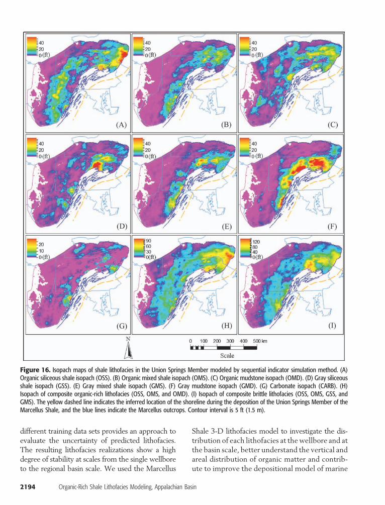
Figure 16. Isopach maps of shale lithofacies in the Union Springs Member modeled by sequential indicator simulation method. (A)Organic siliceous shale isopach (OSS). (B) Organic mixed shale isopach (OMS). (C) Organic mudstone isopach (OMD). (D) Gray siliceousshale isopach (GSS). (E) Gray mixed shale isopach (GMS). (F) Gray mudstone isopach (GMD). (G) Carbonate isopach (CARB). (H)Isopach of composite organic-rich lithofacies (OSS, OMS, and OMD). (I) Isopach of composite brittle lithofacies (OSS, OMS, GSS, andGMS). The yellow dashed line indicates the inferred location of the shoreline during the deposition of the Union Springs Member of theMarcellus Shale, and the blue lines indicate the Marcellus outcrops. Contour interval is 5 ft (1.5 m).

different training data sets provides an approach toevaluate the uncertainty of predicted lithofacies.The resulting lithofacies realizations show a highdegree of stability at scales from the single wellboreto the regional basin scale. We used the Marcellus

2194 Organic-Rich Shale Lithofacies Modeling, Appalachian Ba

Shale 3-D lithofacies model to investigate the dis-tribution of each lithofacies at thewellbore and atthe basin scale, better understand the vertical andareal distribution of organic matter and contrib-ute to improve the depositional model of marine

sin

Figure 17. Isopach maps of shale lithofacies in the entire interval of the Marcellus Shale modeled by the sequential indicator simulationmethod and the overlaying contour lines of the thickness ratio of each lithofacies to the entire Marcellus Shale. (A) Organic siliceous shaleisopach (OSS). (B) Organic mixed shale isopach (OMS). (C) Organic mudstone isopach (OMD). (D) Gray siliceous shale isopach (GSS).(E) Gray mixed shale isopach (GMS). (F) Gray mudstone isopach (GMD). (G) Carbonate isopach (CARB). (H) Isopach of compositeorganic-rich lithofacies (OSS, OMS, and OMD). (I) Isopach of composite brittle lithofacies (OSS, OMS, GSS, and GMS).The red and yellowdashed lines indicate the inferred locations of the shorelines during the deposition of the Oatka Creek and the Union Springs Members,respectively, and the blue lines indicate the Marcellus outcrops. The color-filled contour interval is 5 ft (1.5 m), and the contour intervalfor thickness ratio is 0.1.

organic-rich mudrock, assist in the design of hori-zontal drilling trajectories and location of stimula-tion activity by identifying intervals of organic-rich

and brittle units, and provide input parameters forthe simulation of gas flow and production in mud-rock (e.g., porosity, permeability, and fractures).

Wang and Carr 2195

Figure 18. Relative proportions of Marcellus Shale lithofacies defined directly by ternary plots of core data (A) and pulsed neutronspectroscopy (PNS) logs (B) compared to proportions of predicted lithofacies from conventional log suites at multiple scales using thecore training data set (C) and PNS log training data set (D). In panels C and D, orange column: the predicted lithofacies in wells; greencolumn: upscaled lithofacies in cells penetrated by wells; purple column: lithofacies in all the three-dimensional cells. OSS = organicsiliceous shale isopach. OMS = organic mixed shale isopach; OMD = organic mudstone isopach; GSS = gray siliceous shale isopach; GMS =gray mixed shale isopach; GMD = gray mudstone isopach; CARB = carbonate isopach.

For the last 8 yr, Marcellus Shale explorationand development activity has increased significantlywith drilling of more than 12,000 horizontal andvertical wells, resulting in a rapid increase in shalegas production. Average monthly Marcellus Shalegas production for the first 6 months of productionfor 1864 horizontal wells drilled between 2004 and2011 in West Virginia and Pennsylvania indicatestwo core areas of gas production (Figure 22). Onearea is in north-central West Virginia and south-west Pennsylvania, and the other is in northeastern

2196 Organic-Rich Shale Lithofacies Modeling, Appalachian Ba

Pennsylvania. These regions of higher Marcellusgas production show a strong relationship in mul-tiple realizations, with an increased thickness ofmodeled composite organic-rich lithofacies (OSS,OMS, andOMD) and composite brittle lithofacies(OSS,OMS,GSS, andGMS) predicted by the 3-Dlithofacies models using either the core trainingset or the PNS training set (Figures 20, 21). Thearea of generally lower production located in cen-tral Pennsylvania shows a thinner isopach of com-posite organic-rich and brittle lithofacies predicted

sin

Figure 19. Fence diagrams showing the similarities and differences of Marcellus Shale lithofacies models based on core-predictedMarcellus Shale lithofacies (A) and three realizations of pulsed neutron spectroscopy–predicted lithofacies (B–D). The fence diagramswere zoomed into Pennsylvania to better display details of Marcellus Shale lithofacies. Geocell dimensions are scaled at 108 layersranging from 0 to 3 ft (0–1 m) vertically and 1500 × 1500 ft (460 m) horizontally. Cells are coded by lithofacies: organic siliceous shale,red; organic mixed shale, dark blue; organic mudstone, brown; gray sileous shale, orange; gray mixed shale, green; gray mudstone, gray;and carbonate, light blue.

by the same 3-D lithofacies models (Figures 20,21). This area in central Pennsylvania is also an areawhere the lowerMarcellus Shale unit (UnionSpringsMember) is thinner (Figure 1). In general, the litho-facies modeling at the regional scale may providesome geologic and engineering insight into variationsin the productivity of the Marcellus Shale in theAppalachian Basin. Although not an unexpectedresult, it appears that, for theMarcellus, both gas inplace and reservoir response to stimulation are crit-ical factors in well productivity. We believe that, inareas such as the Appalachian Basin, with an abun-dance of wells with conventional logs, these crit-ical unconventional reservoir parameters can bequantifiers and mapped with models based onpetrophysical responses.

In addition, at a smaller near wellbore scale,variations in lithofacies seem to be significant. Al-though the horizontal scale (1500 ft [457m]) is notdesigned for geosteering, a vertical panel extractedfrom the 3-D lithofacies model shows the impor-tance of understanding the vertical and lateral dis-tributions of lithofacies for the design of horizontaldrilling trajectories and location of stimulation ac-tivity (Figure 23). The regional model could bereadily adapted at a finer scale with detailed controlprovided by 3-D seismic data.

Deposition and accumulation of an organic-richmudrock is a complex process controlled by theinteraction of terrigenous sediment setting rate,sediment dilution, organic matter productivity, andorganic matter preservation and decomposition

Wang and Carr 2197

Figure 20. Isopach maps of the composite organic lithofacies (organic siliceous shale, organic mixed shale, and organic mudstoneisopach) predicted by the three-dimensional lithofacies models using the core training set (A), and multiple realization using the pulsedneutron spectroscopy training set (B–D). All realizations show similar patterns, but areas of relatively thick organic-rich lithofacies arelocated in the areas of north-central West Virginia–southwest Pennsylvania and northeastern Pennsylvania and south-central New York.The blue lines indicate the Marcellus outcrops, and the contour interval is 10 ft (3 m).

(Sageman et al., 2003; Arthur and Sageman, 2005;Aplin andMacquaker, 2011). Given a similar sourcearea, the sedimentation rate in the basin is primarily

2198 Organic-Rich Shale Lithofacies Modeling, Appalachian Ba

influenced by the distance from the shorelineand the bathymetry of the seafloor (Figure 24).Continued subsidence and compaction creates

sin

Figure 21. Isopach maps of the composite brittle lithofacies (siliceous shale, organic mixed shale, gray siliceous shale isopach. and graymixed shale isopach) predicted by the three-dimensional lithofacies models using a core training set (A), and multiple realization using apulsed neutron spectroscopy training set (B–D). All realizations show similar patterns, areas, or relatively thin brittle lithofacies and areconcentrated in west-central Pennsylvania. The blue lines indicate the Marcellus outcrops, and the contour interval is 10 ft (3 m).

accommodation space, resulting in the thickest ac-cumulation of the Marcellus Shale on the easternmargin of the Appalachian Basin (Figure 11).

The organic-rich OSS lithofacies displays acrescent shape crossing the entire basin from north-east to southwest, which is slightly basinward and

Wang and Carr 2199

Figure 22. Bubble map of monthly average Marcellus Shale gas production (mmcf) for the first 6 months of production from horizontalwells in Pennsylvania and West Virginia overlain on the Marcellus Shale isopach of modeled composite organic-rich lithofacies (A) andthe composite brittle lithofacies (B). The filled color and the radius indicate the values of average gas production; the lower color bar isfor production data and the unit is mmcf/month; the upper color bar is for isopach maps.

Figure 23. An extracted cross section of a three-dimensionallithofacies geomodel showing a potential wellbore trajectory inthe dipping organic-rich siliceous shale facies (red) of the lowerMarcellus Shale. Hydraulic fracture stimulation would probablyextend toward the Onondaga Limestone at the base of the Mar-cellus and upward to the relatively thick carbonate facies (lightblue). Geocell dimensions are scaled at 108 layers ranging from0 to 3 ft (0–1m) vertically and 1500 × 1500 ft (460 m) horizontally.Cells are coded by lithofacies: organic siliceous shale, red; organicmixed shale, dark blue; organic mudstone, brown; gray siliceousshale, orange; gray mixed shale, green; gray mudstone, gray; andcarbonate, light blue.

2200 Organic-Rich Shale Lithofacies Modeling, Appalachian Ba

approximately parallel with the depositional pat-terns as defined by the isopach maps of the On-ondaga and Purcell limestone units (Figures 14A,B; 15A; 16A; 17A). In the Oatka Creek Member,the OSS lithofacies was deposited mainly in thejunction of Pennsylvania,West Virginia, andOhio,and secondary in northwestern Pennsylvania andmiddle New York (Figures 14A, 15A). The localbreaks of the organic-rich OSS crescent resultedfrom the lack of organic matter and thus were richinGSS. In theUnion SpringsMember, the crescentof OSS lithofacies is more clear and continuouswith similar thickness, but with a higher percent-age of the unit thickness (Figures 14B, 16A). Inaddition, as shown in cross section (Figure 14C)and isopach maps (Figures 15A, 16A), the depo-sition center of OSS lithofacies moved toward thenorthwest from the bottom Union Springs Memberto the top of theOatkaCreekMember, which couldbe explained by the effect of the basinward pro-gradation of the units. This explanation can also beconfirmed by the similar shifting ofGMD lithofaciesin theMarcellus Shale (Figures 14C, 15F, 16F). TheGMD lithofacies in the Oatka Creek Member and

sin

Figure 24. Conceptual cross section of foreland basin showing the variation of sediment setting rate, organic matter productivity, andorganic matter preservation and decomposition perpendicular to the shoreline (modified from Arthur and Sageman, 2005). The twoarrows indicate the water-column mixing resulting from upwelling and ocean currents. The organic matter productivity includes primarybioproductivity in situ and transportation of organic matter from surrounding areas; the sediments could come from terrigenous clasticsand marine biogenic detritus; sediment burial degree indicates the preservation potential of organic matters, which is related to sed-iments and hydrodynamic energy; organic matter decomposition is associated with oxidation and microbial activity.

the Union Springs Member presented similar cres-cent shapeswithOSS lithofacies, but the depositioncenter of GMD lithofacies was farther to the east.

The density of quartz is less than illite andchlorite; however, the far larger surface area andthe special layer structure of clay minerals tend toabsorb water, organic matter, and other clay min-erals, which decrease the settling velocity. There-fore, the deposition center of quartz-rich shale litho-facies should be closer to the shoreline than theclay-rich shale lithofacies. However, the isopachmaps in the Oatka Creek Member and the UnionSprings Member demonstrated that the depositioncenter of OMD lithofacies was located to both theeast and west of OSS lithofacies (Figures 14A, B;15C; 16C; 17C). Several factors contributed to thisdifference, but the most important reason couldbe the source of quartz and the medium of trans-portation. The quartz could come from terrigenousclastics or marine biogenic detritus, and the ter-rigenous clastics could be transported by fluvial oreolian systems.With regard to the organic-rich shale,

the eolian transportation of terrigenous quartz andthe marine biogenic quartz in situ are believed tobe a more important factor than the fluvial trans-portation of terrigenous quartz. The trends of higherquartz concentration along with higher TOC con-tent in Figure 4A also support the important func-tion of marine biogenic quartz in organic-rich shaledeposition. The clay minerals of OMD lithofaciesto the east of OSS lithofacies were mainly trans-ported by fluvial system; on the contrary, the west-ern OMD lithofacies accept clay minerals by eoliantransportation.

Compared to the other lithofacies, the carbonate-rich lithofacies was more isolated, especially in theOatkaCreekMember (Figures 15B, E; 16B, E ; 17B,E). In the northeast of the Appalachian Basin, theOMS and GMS lithofacies became richer and con-tinuous. Based on the isopach maps (Figures 15–17) and the 3-D view (column 3 in Figure 14), thecarbonate-rich lithofacies tends to be located ba-sinward of the GMD lithofacies, where a progra-dational delta could form a high dip angle. The

Wang and Carr 2201

summed isopach maps of the three organic-richlithofacies (OSS, OMS, and OMD) illustrate thatthe content of organic matter was high in northernWest Virginia, southwestern and northern Penn-sylvania, and southeastern New York (Figures 15H;16H; 17H). The natural gas in place should behigher in these areas, if the maturity was similar.The OSS, OMS, GSS, and GMD lithofacies con-tained more quartz and limestone, so the shale wasmore brittle than clay-rich shale. These four litho-facies were added together to make up the brittlelithofacies in the Appalachian Basin (Figures 15I;16I; 17I). Compared to the organic-rich lithofacies,the brittle lithofacies was more centralized in thecentral and eastern Appalachian Basin. For exam-ple, in southwestern West Virginia and northeast-ern Ohio, the Marcellus Shale showed an increasein organic richness but was more ductile becauseof the high clay concentration, so it is more diffi-cult to stimulate production to yield high produc-tion rates.

SUMMARY

• Marcellus Shale lithofacies can be defined fromcore and PNS logs in terms of mineral compo-sition and organic matter richness, clay percent-age, the ratio of quartz and carbonate, and TOCcontent. These parameters are the three keycriteria for recognizing and defining seven Mar-cellus Shale mudrock lithofacies.

• The artificial neural network using two inde-pendently derived training data sets from coredata and PNS logs was used to predict MarcellusShale lithofacies through the abundant con-ventional logs available across the AppalachianBasin. In place of unmodified log data, petro-physical analysis was used to derive eight nor-malized parameters as the input variables formthe ANN and reduce local effects of the well-bore environment and the variable presence ofminerals with strong petrophysical effects suchas pyrite and barite.

• Regional and local faults were interpreted fromthe integration of well logs, contour maps ofsubsea elevation of formation tops, and 3-D

2202 Organic-Rich Shale Lithofacies Modeling, Appalachian Ba

seismic data. A regional 3-D structuralmodel wasbuilt as the framework to constrain theMarcellusShale 3-D lithofacies model.

• Sequential indicator simulation with a suitablevariogram model of each lithofacies performedwell for the stochastic modeling of MarcellusShale lithofacies. Two-dimensional ordering ofMarcellus lithofacies using relative quartz to clayand organic richness resulted in TGS not beingas effective as lithofacies modeling.

• The distribution of Marcellus Shale lithofaciesseems to be strongly influenced by a complexinteraction of sediment dilution, organic matterproductivity, and organic matter preservationand decomposition. This is illustrated by thecrescent shape and offshore position, which par-allels the inferred Marcellus shoreline in theeastern Appalachian Basin.

• The two different kinds of ANN models (orclassifiers), trained by core- and PNS-trainingdata sets, respectively, generated very similarresults for the 3-D geocellular model of Mar-cellus Shale lithofacies at multiple scales fromthe wellbore to the small regions of the basin.

• At the basin scale, the distribution of gas pro-duction from theMarcellus Shale shows a strongrelationship to multiple realizations showing athicker isopach of composite organic-rich litho-facies (OSS, OMS, and OMD) and compositebrittle lithofacies (OSS, OMS, GSS, and GMS)predicted by the 3-D lithofacies models. Local3-D lithofacies models of the Marcellus Shaleconstrained with sufficient data may be helpfulfor designing the trajectory of horizontal wellsand placement of hydraulic fracturing in shale-gas exploration and production.

REFERENCES CITED

Akatsuka, K., 2000, 3-D geological modeling of a carbonatereservoir, utilizing open-hole log response: Porosity andpermeability—Lithofacies relationship: 9th Abu DhabiInternational Petroleum Exhibition and Conference,Abu Dhabi, U.A.E., October 15–18, 2000, SPE Paper87239, 11 p.

Allard, D., 1994, Simulating a geological lithofacies with re-spect to connectivity information using the truncated

sin

Gaussian model, inM. Armstrong and P. A. Dowd, eds.,Geostatistical simulation: Dordrecht, Netherlands,Kluwer Academic, p. 197–211.

Aplin, A. C., and J. H. S. Macquaker, 2011, Mudstone diver-sity:Origin and implications for source, seal, and reservoirproperties in petroleum systems: AAPG Bulletin, v. 95,no. 12, p. 2031–2059, doi:10.1306/03281110162.

Arthur, M. A., and B. B. Sageman, 2005, Sea-level control onsource-rock development: Perspectives from the Holo-cene Black Sea, the mid-Cretaceous Western InteriorBasin of North America, and the Late Devonian Appa-lachian Basin, in N. B. Harris and B. Pradier, eds., Thedeposition of organic carbon-rich sediments: Models,mechanisms and consequences: SEPM Special Publica-tion 82, p. 35–59.

Berteig, V., J. Helgeland, E. Mohn, T. Langeland, and D. vander Wel, 1985, Lithofacies prediction from well data:Transactions of the 26th Society of Petrophysicists andWell Log Analysts Annual Logging Symposium, 25 p.

Beucher, H. A., A. Galli, G. Le Loc’h, and C. Ravenne, 1993,Including a regional trend in reservoir modeling usingthe truncated Gaussian method, in A. Soares, ed., Geo-statistics Troia ’92: Dordrecht, Netherlands, Kluwer Ac-ademic, v. 1, p. 555–566.

Bowker, K. A., 2007, Barnett Shale gas production, FortWorth Basin: Issues and discussion: AAPG Bulletin, v. 91,no. 4, p. 523–533, doi:10.1306/06190606018.

Boyce, M. L., and T. R. Carr, 2010, Stratigraphy and petro-physics of the Middle Devonian black shale interval inWest Virginia and southwest Pennsylvania: AAPG Searchand Discovery article 10265, accessed May 22, 2013,http://www.searchanddiscovery.com/documents/2010/10265boyce/poster01.pdf.

Brett, C. E., and G. C. Baird, 1996, Middle Devonian sedi-mentary cycles and sequences in the northern Appala-chian Basin: Geological Society of America Special Pa-per 306, p. 213–241.

Bridge, J. S., G. A. Jalfin, and S. M. Georgieff, 2000, Geom-etry, lithofacies, and spatial distribution of Cretaceousfluvial sandstone bodies, San Jorge Basin, Argentina:Outcrop analog for the hydrocarbon-bearing ChubutGroup: Journal of Sedimentary Research, v. 70, no. 2,p. 341–359, doi:10.1306/2DC40915-0E47-11D7-8643000102C1865D.

Carr, T. R., G. Wang, M. L. Boyce, and A. Yanni, 2011,Understanding controls on deposition of organic con-tent in the Middle Devonian organic-rich shale inter-vals of West Virginia andwestern Pennsylvania: GeologicalSociety of America Abstracts with Programs: Northeast(46th Annual) and North-Central (45th Annual) JointMeeting, Pittsburgh, March 20–22, 2011, v. 43, no. 1,50 p.

Chang, H., D. C. Kopaska-Merkel, H. Chen, and S. R. Durrans,2000, Lithofacies identification using multiple adaptiveresonance theory neural networks and group decisionexpert system: Computers & Geosciences, v. 26, no. 5,p. 591–601, doi:10.1016/S0098-3004(00)00010-8.

Curtis, M. E., R. J. Ambrose, C. H. Sondergeld, and C. S. Rai,2010, Structural characterization of gas shales on themicro- and nanoscales: Canadian Unconventional

Resources and International Petroleum Conference, Cal-gary, Alberta, Canada, October 19–21, 2010, SPE Paper137, 15 p.

Deutsch, C. V., 2002, Geostatistical reservoir modeling: NewYork, Oxford University Press, 376 p.

Doyle, J., andM. Sweet, 1995, Three-dimensional distributionof lithofacies, bounding surfaces, porosity, and perme-ability in a fluvial sandstone: Gypsy Sandstone of north-ern Oklahoma: AAPG Bulletin, v. 79, no. 1, p. 70–96.

Dubois, M. K., G. C. Bohling, and S. Chakrabarti, 2007,Comparison of four approaches to a rock facies classifi-cation problem: Computers & Geosciences, v. 33, no. 5,p. 599–617, doi:10.1016/j.cageo.2006.08.011.

Emery, X., and J. Cornejo, 2010, Truncated Gaussian simu-lation of discrete-valued, ordinal coregionalized vari-ables: Computers & Geosciences, v. 36, no. 10, p. 1325–1338, doi:10.1016/j.cageo.2010.03.013.

Ettensohn, F. R., and L. S. Barron, 1981a, Tectonoclimaticmodel for origin of Devonian–Mississippian black gasshales of east-central United States: AAPG Bulletin, v. 65,p. 1–83.

Ettensohn, F. R., and L. S. Barron, 1981b, Depositional modelfor the Devonian–Mississippian black shales of NorthAmerica: A paleoclimatic-paleogeographic approach, inT. G. Roberts, ed., GSA Cincinnati ’81 Field Trip Guide-books: Economic geology, structure: Falls Church, Amer-ican Geological Institute, v. 2, p. 344–361.

Falivene, O., P. Arbues, A. Gardiner, G. Pickup, J. A. Munoz,and L. Cabrera, 2006, Best practice stochastic faciesmodeling from a channel-fill turbidite sandstone analog(the Quarry outcrop, Eocene Ainsa Basin, northeast Spain):AAPG Bulletin, v. 90, no. 7, p. 1003–1029, doi:10.1306/02070605112.

Gao, D., R. C. Shumaker, and T. H. Wilson, 2000, Along-axis segmentation and growth history of the Rometrough in the central Appalachian Basin: AAPG Bulletin,v. 84, p. 75–99.

Haldorsen, H. H., and D. M. Chang, 1986, Notes on stochas-tic shales: From outcrop to simulation model, in L. W.Lake and H. B. Caroll, eds., Reservoir characterization:New York, Academic Press, p. 445–485.

Hickey, J. J., and B. Henk, 2007, Lithofacies summary of theMississippian Barnett Shale, Mitchell 2 T.P. Sims Well,Wise County, Texas: AAPGBulletin, v. 91, no. 4, p. 437–443, doi:10.1306/12040606053.

Ibach, L. E. J., 1982, Relationship between sedimentationrate and total organic carbon content in ancient marinesediments: AAPG Bulletin, v. 66, p. 170–188.

Jarvie, D. M., R. J. Hill, T. R. Ruble, and R. M. Pollastro,2007, Unconventional shale-gas systems: The Mississip-pian Barnett Shale of north-central Texas as one modelfor thermogenic shale-gas assessment: AAPG Bulletin,v. 91, no. 4, p. 475–499, doi:10.1306/12190606068.

Javadpour, F., 2009, Nanopores and apparent permeabilityof gas flow in mudrocks (shales and siltstone): Journalof Canadian Petroleum Technology, v. 48, p. 16–21.

Jonk, R., K. Potma, M. Davie, and N. Austin, 2012, Mud-stone lithofacies within a sequence-stratigraphic frame-work: Key to mapping shale-gas rock properties in theHorn River Basin, Canada: AAPG Search and Discovery

Wang and Carr 2203

article 90142, accessed May 22, 2013, http://www.searchanddiscovery.com/abstracts/html/2012/90142ace/abstracts/jonk.htm.

Koesoemadinata, A., G. El-Kaseeh, N. Banik, J. C. Dai, M.Egan, A. Gonzalez, and K. Tamulonis, 2011, Seismic res-ervoir characterization in Marcellus Shale: Proceedings ofSociety of Exploration Geophysicists San Antonio 2011Annual Meeting, New York, Curran Associates, Inc.,p. 3700–3704.

Lash, G. G., 2008, The influence of basin dynamics on depo-sitional patterns of the Middle Devonian MarcellusShale, western New York and northwestern Pennsylva-nia (abs.): AAPGAnnual Convention, San Antonio, Texas,April 20–23, 2008, v. 17, p. 116.

Lash, G. G., and T. Engelder, 2011, Thickness trends and se-quence stratigraphy of the Middle Devonian MarcellusFormation, Appalachian Basin: Implications for Acadianforeland basin evolution: AAPG Bulletin, v. 95, no. 1,p. 61–103, doi:10.1306/06301009150.

Laubach, S. E., J. E. Olson, and M. R. Gross, 2009, Mechan-ical and fracture stratigraphy: AAPG Bulletin, v. 93,no. 11, p. 1413–1426, doi:10.1306/07270909094.

Loucks, R. G., and S. C. Ruppel, 2007, Mississippian BarnettShale: Lithofacies and depositional setting of a deep-water shale-gas succession in the Fort Worth Basin,Texas: AAPG Bulletin, v. 91, no. 4, p. 579–601, doi:10.1306/11020606059.

Loucks, R. G., R. M. Reed, S. C. Ruppel, and U. Hammes,2012, Spectrum of pore types and networks in mudrocksand a descriptive classification for matrix-related mud-rock pores: AAPG Bulletin, v. 96, no. 6, p. 1071–1098,doi:10.1306/08171111061.

Marshak, S., 2010, Essentials of geology, 3d ed.: New York,W. W. Norton & Company Limited, 648 p.

Mavko, G., 2010, Rock physics of shales and source rocks:Pacific Coast Section Society of Exploration Geophysi-cists, accessed May 7, 2012, http://pcs-seg.org/PCSSlides/MavkoMarch2010.pdf.

Perez, R., 2009, Quantitative petrophysical characterizationof the Barnett Shale in Newark east field, FortWorth Ba-sin: Master’s thesis, University of Oklahoma, Norman,Oklahoma, 132 p.

Porta, G. D., J. A. M. Kenter, A. Immenhauser, and J. R.Bahamonde, 2002, Lithofacies character and architec-ture across a Pennsylvanian inner-platform transect(Sierra De Cuera, Asturias, Spain): Journal of Sedimen-tary Research, v. 72, no. 6, p. 898–916, doi:10.1306/040902720898.

Qi, L., and T. R. Carr, 2006, Neural network prediction ofcarbonate lithofacies from well logs, Big Bow and SandArroyo Creek fields, southwest Kansas: Computers &Geosciences, v. 32, no. 7, p. 947–964, doi:10.1016/j.cageo.2005.10.020.

Qi, L., T. R. Carr, and R. H. Goldstein, 2007, Geostatisticalthree-dimensional modeling of oolite shoals, St. LouisLimestone, southwest Kansas: AAPG Bulletin, v. 91,no. 1, p. 69–96, doi:10.1306/08090605167.

Ruppel, S. C., R. Harbor, R. Loucks, G. Frebourg, and H.Rowe, 2012, Eagle Ford facies architecture: Interplayof proximal and distal carbonate and siliciclastic sediment

2204 Organic-Rich Shale Lithofacies Modeling, Appalachian Ba

sources: AAPG Search and Discovery article 90142, ac-cessed May 22, 2013, http://www.searchanddiscovery.com/abstracts/html/2012/90142ace/abstracts/rup.htm.

Sageman, B. B., A. E.Murphy, J. P.Werne, C. A. VerStraeten,D. J. Hollander, and T. W. Lyons, 2003, A tale of shales:The relative roles of production, decomposition, anddilution in the accumulation of organic-rich strata, Middle–Upper Devonian, Appalachian Basin: Chemical Geology,v. 195, p. 229–273, doi:10.1016/S0009-2541(02)00397-2.

Schlumberger, 2011, accessed May 8, 2012, http://www.slb.com/services/software/geo/petrel/geomodeling/facies_modeling.aspx.

Singh, P., 2008, Lithofacies and sequence-stratigraphic frame-work of the Barnett Shale, northeastern Texas: Ph.D. dis-sertation, University of Oklahoma, Norman, Oklahoma,181 p.

Smith, L. B., 2010, Shallow transgressive onlap model forOrdovician and Devonian organic-rich shales, New YorkState: AAPG Search and Discovery article 90116, ac-cessed May 22, 2013, http://www.searchanddiscovery.com/abstracts/pdf/2010/eastern/abstracts/ndx_smith.pdf.

Smith, T., and J. Leone, 2010, PAPG/PTTC Spring Fieldtripand Core Workshop - “A tale of two shales”: accessedMay 22, 2013, http://www.papgrocks.org/publications.html.

Suess, E., 1980, Particulate organic carbon flux in the ocean:Surface productivity and oxygen utilization: Nature,v. 288, p. 260–263, doi:10.1038/288260a0.

Teichert, C., 1958, Concepts of facies: AAPG Bulletin, v. 42,no. 11, p. 2718–2744.

U.S. Geological Survey, 2004, Geologic provinces of theUnited States: Appalachian Highlands province: ac-cessed May 7, 2012, http://3dparks.wr.usgs.gov/nyc/valleyandridge/valleyandridge.htm.

Vallejo, J. S., 2010, Prediction of lithofacies in the thinly bed-ded Barnett Shale, using probabilistic methods and clus-tering analysis through GAMLS TM (geologic analysisvia maximum likelihood system): Master’s thesis, Uni-versity of Oklahoma, Norman, Oklahoma, 184 p.

VerStraeten, C. A., 2007, Basinwide stratigraphic synthesisand sequence stratigraphy, upper Pragian, Emsian andEifelian stages (Lower to Middle Devonian), Appala-chian Basin: Geological Society (London) Special Publi-cation 278, p. 39–81, doi:10.1144/SP278.3.

Walker-Milani, M. E., 2011, Outcrop lithostratigraphy andpetrophysics of the Middle Devonian Marcellus Shalein West Virginia and adjacent states: Master’s thesis, WestVirginia University, Morgantown, West Virginia, 130 p.

Wang, G., and T. R. Carr, 2012a, Black shale lithofaciesidentification and distribution model of Middle Devo-nian intervals in the Appalachian Basin: AAPG Searchand Discovery article 90142, accessed May 22, 2013,http://www.searchanddiscovery.com/abstracts/html/2012/90142ace/abstracts/wang3.htm.

Wang, G., and T. R. Carr, 2012b, Methodology of organic-rich shale lithofacies identification and prediction: Acase study from Marcellus Shale in the Appalachian Ba-sin: Computers & Geosciences, v. 49, p. 151–163,doi:10.1016/j.cageo.2012.07.011.

sin

Wang, G., and T. R. Carr, 2012c, Marcellus Shale lithofaciesprediction by multiclass neural network classification inthe Appalachian Basin: Mathematical Geosciences, v. 44,p. 975–1004, accessed October 2, 2012, http://www.springerlink.com/openurl.asp?genre=article&id=doi:10.1007/s11004-012-9421-6.

Werne, J. P., B. B. Sageman, T. W. Lyons, and D. J. Hollander,2002, An integrated assessment of a “type euxinic” deposit:Evidence for multiple controls on black shale deposition inthe Middle Devonian Oatka Creek Formation: AmericanJournal of Science, v. 302, p. 110–143, doi:10.2475/ajs.302.2.110.

Wong, P. M., T. D. Gedeon, and I. J. Taggart, 1995, The useof fuzzy ARTMAP for lithofacies classifications: A com-parison study: Transactions of the 36th Society of Petro-physicists and Well Log Analysts Annual LoggingSymposium.

Woodrow, D. L., and W. D. Sevon, 1985, The Catskill Delta:Geological Society of America Special Paper 201,p. 39–49.

Yao, T., and A. Chopra, 2000, Integration of seismic data at-tribute map into 3-D facies modeling: Journal of Petro-leum Science and Engineering, v. 27, p. 69–84, doi:10.1016/S0920-4105(00)00048-6.

Yarus, J. M., and R. L. Chambers, 1994, Stochastic modelingand geostatistics: Principles, methods, and case studies:AAPG Computer Applications in Geology 3, 379 p.

Zhou, J., P. F. Rush, A. Sridhar, and R. Miller, 2012, Theanatomy of Middle Devonian Marcellus Shale, Appala-chian Basin: A scheme ofmudstone classification and itsimplications for shale gas exploration: AAPG Searchand Discovery article 90142, accessed May 22, 2013,http://www.searchanddiscovery.com/abstracts/html/2012/90142ace/abstracts/zhou.htm.

Wang and Carr 2205