
OPTIMUM WATER NETWORK DESIGN FOR MULTIPURPOSE...
190
OPTIMUM WATER NETWORK DESIGN FOR MULTIPURPOSE BATCH PLANTS WITH A DETAILED ELECTRODIALYSIS REGENERATION MODEL Nsunda Christie Bazolana (572003) “A dissertation submitted to the Faculty of Engineering and the Built Environment, University of the Witwatersrand, Johannesburg, in fulfilment of the requirements for the degree of Master of Science in Engineering” Supervised by: Professor Thokozani Majozi June 2018
Transcript of OPTIMUM WATER NETWORK DESIGN FOR MULTIPURPOSE...

OPTIMUM WATER NETWORK DESIGN FOR
MULTIPURPOSE BATCH PLANTS WITH A DETAILED
ELECTRODIALYSIS REGENERATION MODEL
Nsunda Christie Bazolana
(572003)
“A dissertation submitted to the Faculty of Engineering and the Built Environment,
University of the Witwatersrand, Johannesburg, in fulfilment of the requirements for
the degree of Master of Science in Engineering”
Supervised by: Professor Thokozani Majozi
June 2018

ii
Declaration
I declare that this dissertation is my own unaided work. It is being submitted for the Degree
of Master of Science in Chemical Engineering to the University of the Witwatersrand,
Johannesburg. It has not been submitted before for any degree or examination to any other
University.
………………………………………………………………………………………………
(Signature of Candidate)
………………………day of……………………..year……………..

iii
Abstract
Stringent environmental regulations and economic expansion in the recent decades
has justified the need for sustainable water usage in the process industry. The usage
of water in multipurpose batch plants is essential in cleaning operations to ensure the
integrity of various tasks processed in multipurpose units by avoiding contamination
between consecutive batches. This usually requires a considerable amount of water
while generating highly toxic effluents. The minimization of water in batch plants is
achieved through direct, indirect and regeneration reuse. These techniques are mainly
dependent on the schedule of the plant and a flexible schedule usually guarantees an
increase in water saving opportunities. While direct and indirect reuse requires capital
investments, regeneration reuse involves additional operational costs through the
consumption of intensive amount of energy. It is therefore vital to capture the trade-
off between water and energy usage and explore their respective cost implications.
This work presents a Mixed Integer Nonlinear Programming (MINLP) formulation
that simultaneously optimizes the production schedule and utility consumption in
multipurpose batch plants. The amount of wastewater generated in batch operations is
minimized through the exploration of direct, indirect, and regeneration reuse
opportunities within the plant. Water regeneration is achieved through partial
purification of highly contaminated wastewater using electrodialysis. A design model
for electrodialysis is included in the formulation in order to allow for simultaneous
optimization of water and energy use in the regenerator. The formulation is first
applied to two examples from literature for validation. Freshwater savings of 37.4 %
and 41.1% are achieved in each literature example while maintaining the revenue at
its maximum value. The efficiency of the designed regenerators with respect to their
energy consumption is evaluated by comparing the proposed technique with a case
where the minimization of energy is not considered. A reduction in energy
consumption by 31.6 % and 9.8% for both examples is respectively observed. A

iv
study is then undertaken at Amul plant, one of the biggest dairy in the world, in order
to assess the practicality of the formulation. The formulation is applied to the raw
milk receiving department (RMRD) where the highest amount of freshwater is
consumed. Freshwater and energy savings of 38 % and 95.2% are achieved under the
consideration of a single quality of water streams. An economic analysis of the
integrated water network is performed and 20 % reduction in the total operating cost
of the RMRD is achieved through the implementation of the proposed water
minimization technique.

v
Dedication
To my parents,
Jean-Pierre Bazolana Mandangi and Veronique Mputu Modiri

vi
Acknowledgments
This work would not have come into existence without the help of my Lord, God
Almighty, who has been my source of knowledge, understanding, provision, strength,
and faith throughout the course of this project. I would like to sincerely thank the
National Research Foundation (NRF) of South Africa for granting me a scholarship
in support of this project. Special words of gratitude go to my supervisor, Professor
Thokozani Majozi, for his guidance and supervision throughout the course of my
master’s studies. He has instilled in me hard work, endurance and taught me to
always embrace criticism as it is an essential component of intellectual growth. His
passion for research has been a great inspiration to me. I would also like to extend my
gratitude to my colleagues and friends from the SPE research group. Your input in
this work, friendship, love, and laughter have contributed to making this research
experience enjoyable.
I am very much indebted to my fiancé, Fortunat Mutunda, who has always been a
shoulder for me to lean on. The many words of encouragements, endless prayers,
discussions and laughter have been a great source of motivation. My sincere thanks
also go to my brothers and sisters: Isaac, Gabrielle, Ime, Tobi, Darwin, Tope; who
have constantly reminded me to stand still in faith and shared the word of God with
me through good and tough times. To my siblings: Glo, Glodi, Louange, Jessah,
Wisdom, Nathalie, Lady, and Rais; thank you for loving, supporting and
understanding me even though I had spent less time with you guys in the past two
years of my master’s study.
This acknowledgment will not be complete without mentioning the moral, financial
and spiritual support of my parents, Jean-Pierre and Veronique Bazolana. Their
willingness to sacrifice everything in support of my dreams has been one of my
greatest motivation for success.

vii
Content
Declaration .................................................................................................................... ii
Abstract ........................................................................................................................ iii
Dedication ..................................................................................................................... v
Acknowledgments ........................................................................................................ vi
Content ........................................................................................................................ vii
List of Figures ............................................................................................................... x
List of Tables ............................................................................................................. xiii
List of Abbreviations ................................................................................................. xiv
INTRODUCTION .......................................................................................... 1-1
1.1 Background ................................................................................................. 1-1
1.2 Motivation for the study .............................................................................. 1-3
1.3 Research objectives ..................................................................................... 1-5
1.4 Problem statement ....................................................................................... 1-6
1.5 Dissertation layout ....................................................................................... 1-6
References .............................................................................................................. 1-7
LITERATURE REVIEW ............................................................................... 2-1
2.1 Introduction ................................................................................................. 2-1
2.2 Batch processes ........................................................................................... 2-2
2.2.1 Background and definition ......................................................... 2-2
2.2.2 Classification of batch processes ................................................ 2-3
2.2.3 Batch operational philosophies .................................................. 2-4
2.2.4 Recipe presentation .................................................................... 2-6
2.2.5 Time representation .................................................................. 2-10
2.3 Scheduling of batch processes ................................................................... 2-12
2.3.1 Definition .................................................................................. 2-12
2.3.2 Mathematical modelling and optimisation ............................... 2-13
2.3.3 Scheduling techniques for batch processes .............................. 2-16
2.3.4 Review of short-term scheduling models for batch processes . 2-20
2.4 Wastewater minimisation in batch plants .................................................. 2-32
2.4.1 Fixed schedule techniques ........................................................ 2-34

viii
2.4.2 Variable schedule techniques ................................................... 2-44
2.5 Consideration of regeneration ................................................................... 2-47
2.5.1 Membrane technologies for wastewater treatment ................... 2-48
2.5.2 Electrodialysis technology ....................................................... 2-51
2.6 Solution approaches to wastewater minimisation problems ..................... 2-54
2.6.1 Convexity in mathematical programming ................................ 2-54
2.6.2 Convexification techniques ...................................................... 2-57
2.6.3 Solution algorithms for MINLP problems ............................... 2-65
2.6.4 Available optimization solvers for MINLP models ................. 2-70
2.7 Summary ................................................................................................... 2-72
References ............................................................................................................ 2-73
MODEL DEVELOPMENT ............................................................................ 3-1
3.1 Introduction ................................................................................................. 3-1
3.2 Scheduling model ........................................................................................ 3-2
3.3 Material balance for the water network ....................................................... 3-3
3.3.1 Water balance constraints for washing operations ..................... 3-3
3.3.2 Storage tanks modelling ............................................................. 3-6
3.4 ED design model ....................................................................................... 3-10
3.5 Sequencing constraints for water network ................................................ 3-16
3.6 Objective function ..................................................................................... 3-23
3.7 Nomenclature ............................................................................................ 3-23
References ............................................................................................................ 3-28
ILLUSTRATIVE EXAMPLES ...................................................................... 4-1
Introduction ................................................................................................. 4-1
Case study I ................................................................................................. 4-1
4.2.1 Computational results and discussion ........................................ 4-5
Case study II .............................................................................................. 4-11
4.3.1 Results and discussions ............................................................ 4-13
References ............................................................................................................ 4-19
INDUSTRIAL CASE STUDY ....................................................................... 5-1
5.1 Introduction ................................................................................................. 5-1
5.2 RMRD process description ......................................................................... 5-4
5.3 Flowsheet simplification and CIP in the RMRD ........................................ 5-5

ix
5.4 Optimization of the RMRD water network ............................................... 5-10
References ............................................................................................................ 5-19
LIMITATIONS AND RECOMMENDATIONS ........................................... 6-1
6.1 Introduction ................................................................................................. 6-1
6.2 Water network limitations ........................................................................... 6-1
6.2.1 Single contaminant ..................................................................... 6-1
6.2.2 Water-using operations ............................................................... 6-2
6.2.3 Water treatment technology ....................................................... 6-2
6.3 Scheduling considerations ........................................................................... 6-4
6.4 Computational intensity .............................................................................. 6-5
6.4.1 CPU time improvement .............................................................. 6-6
References ............................................................................................................ 6-10
CONCLUDING REMARKS .......................................................................... 7-1
Appendices ................................................................................................................ A-1
Appendix A: Scheduling formulation of Seid and Majozi (2012) .................. A-1
x
List of Figures
Figure 1.1 Motivation for the study ...................................................................... 1-5
Figure 2.1 Analogy between continuous and batch processes .............................. 2-3
Figure 2.2 Sequence of tasks in (a) multiproduct and (b) multipurpose batch plants
(Majozi, 2010) ...................................................................................... 2-4
Figure 2.3 STN and SSN representation of a simple batch process (Majozi, 2010) ..
.............................................................................................................. 2-7
Figure 2.4 RTN representation of a batch process (Shaik & Floudas, 2008) ........ 2-8
Figure 2.5 S-graph of a batch production recipe (Sanmarti, et al., 1998) ............. 2-9
Figure 2.6 SEN representation of a batch process (Nie, et al., 2012) ................. 2-10
Figure 2.7 (a) Discrete and (b) Continuous time representation (Majozi, 2010) 2-11
Figure 2.8 Graphical representation of a LP model (Williams, 2013) ................ 2-15
Figure 2.9 Global time interval models (Harjunkoski, et al., 2014) .................... 2-17
Figure 2.10 Global event and unit-specific event based models (Harjunkoski, et al.,
2014) .................................................................................................. 2-18
Figure 2.11 Synchronous and asynchronous slot based representations
(Harjunkoski, et al., 2014) ................................................................. 2-19
Figure 2.12 Precedence-based techniques for event representation (Harjunkoski, et
al., 2014) ............................................................................................ 2-20
Figure 2.13 Optimal event determination framework for (a) profit maximization and
(b) makespan minimization problems (Li & Floudas, 2010) ............. 2-28
Figure 2.14 Scheduling technique of (a) Majozi and Zhu (2001) and (b) Seid and
Majozi (2012b) ................................................................................... 2-31
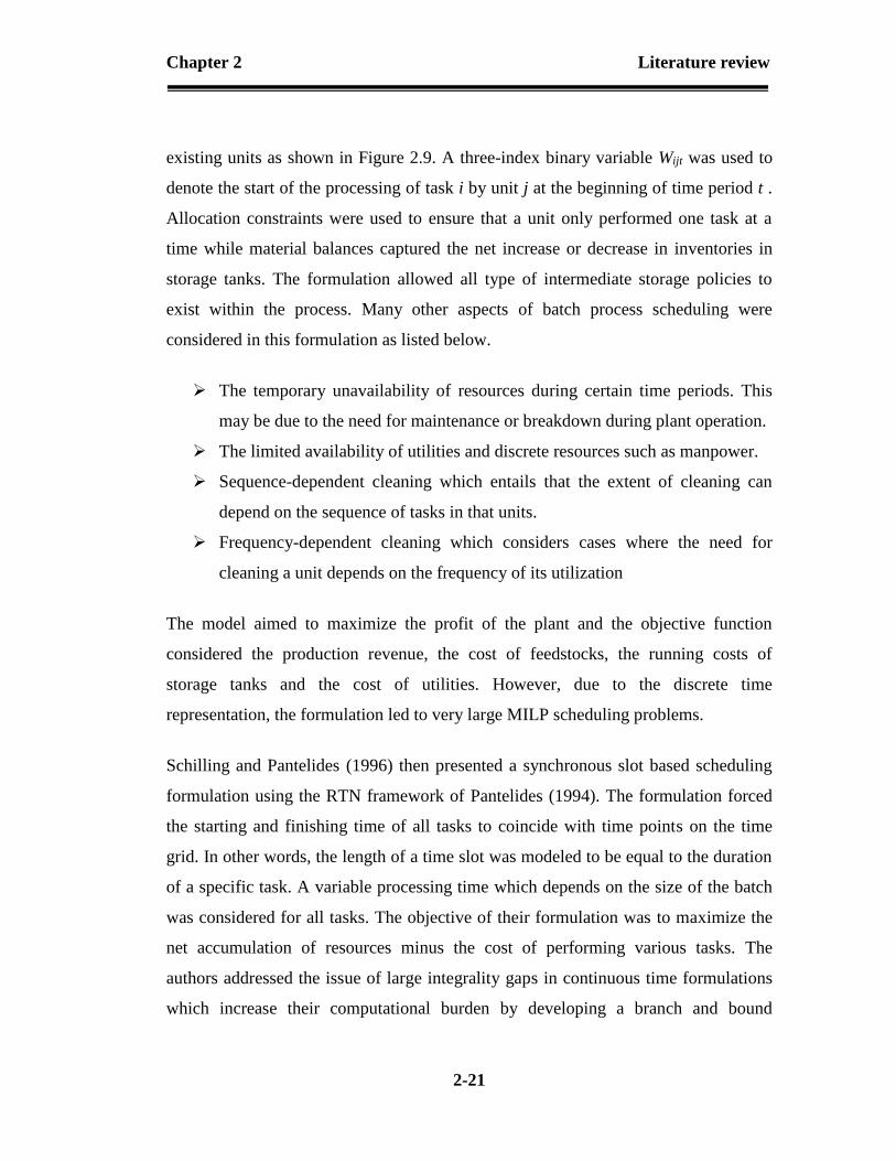
Figure 2.15 Procedure of Seid and Majozi (2012b) to predicting the optimum
number of time points ........................................................................ 2-32
Figure 2.16 Water integration techniques for in batch processes .......................... 2-34
Figure 2.17 Graphical technique of Wang and Smith (1995) for water targeting in
batch processes .................................................................................. 2-36

xi
Figure 2.18 Graphical techniques of Majozi et al. (2006) with (a) time and (b)
concentrations treated as primary constraints. ................................... 2-38
Figure 2.19 Graphical technique of Chen and Lee (2008) .................................... 2-40
Figure 2.20 Principle of a membrane operation .................................................... 2-49
Figure 2.21 Schematic diagram illustrating the principle of ED desalination stack
containing CEMs and AEMs in alternating series (Strathmann, 2004).
........................................................................................................ 2-52
Figure 2.22 Convex and Non-convex regions (Edgar & Himmelblau, 1988) ...... 2-55
Figure 2.23 Comparison between (a) Concave and (b) Convex functions (Edgar &
Himmelblau, 1988) ............................................................................ 2-56
Figure 2.24 A graphical representation of a nonconvex function (Edgar &
Himmelblau, 1988) ............................................................................ 2-57
Figure 2.25 Graphical representation of McCormick (1976) envelopes .............. 2-60
Figure 2.26 α-BB underestimation of a typical nonconvex function g(x) (Lundell, et
al., 2013) ............................................................................................ 2-62
Figure 2.27 Compensation function W(x) and its overestimation Ŵ(x) obtained by
PLFs with (a) three and (b) five breakpoints (Lundell, et al., 2013) . 2-64
Figure 2.28 GBD and OA solution procedure for MINLP models ...................... 2-68
Figure 2.29 Outer approximation (at three points) of a convex function in R1 (Duran
& Grossmann, 1986) .......................................................................... 2-69
Figure 3.1 Water network superstructure for the proposed formulation ............... 3-2
Figure 3.2 Scheduling model concept for batch processes.................................... 3-3
Figure 3.3 Limiting water requirement for each washing operation (Majozi, 2005a)
.............................................................................................................. 3-6
Figure 3.4 Schematic representation of a single-stage electrodialysis regeneration
process ................................................................................................ 3-11
Figure 3.5 Modelling technique for the regenerator operation............................ 3-20
Figure 4.1 State task network representation of the production recipe for case study
I ............................................................................................................ 4-2
Figure 4.2 Gantt chart for case study I ................................................................ 4-10

xii
Figure 4.3 SSN and STN representation for production recipe of case study II . 4-12
Figure 4.4 Gantt chart for case study II ............................................................... 4-18
Figure 5.1 Amul dairy production plant scheme ................................................... 5-2
Figure 5.2 Distribution of water consumption in Amul dairy plant ..................... 5-2
Figure 5.3 Water use distribution in the CIP and floor cleaning sector of Amul
dairy plant ............................................................................................ 5-3
Figure 5.4 Simplified block flow diagram for the RMRD .................................... 5-7
Figure 5.5 STN representation of the RMRD production recipe .......................... 5-7
Figure 5.6 Process flow diagram in the RMRD .................................................... 5-8
Figure 5.7 RMRD plant schedule prior to water integration ............................... 5-14
Figure 5.8 Gantt chart representing the proposed schedule and water network of
Amul RMRD. ..................................................................................... 5-18

xiii
List of Tables
Table 2.1 Classification of membrane operations (Mallevialle, et al., 1996) ........ 2-50
Table 4.1 Production scheduling data for case study I ............................................ 4-3
Table 4.2 Additional scheduling data for case study I ............................................. 4-3
Table 4.3 Process integration data for washing tasks in case study I ...................... 4-3
Table 4.4 Additional parameters for the design and costing of the ED unit and
storage tanks for case study I and II ........................................................ 4-4
Table 4.5 Comparative results for case study I ........................................................ 4-6
Table 4.6 Design specifications of the ED regenerator for case study I .................. 4-7
Table 4.7 Results from black-box and detailed modelling approaches ................... 4-9
Table 4.8 Production scheduling data for case study II ......................................... 4-13
Table 4.9 Additional scheduling data for case study II ......................................... 4-14
Table 4.10 Process integration data for tasks requiring washing for case study II .. 4-14
Table 4.11 Detailed results for case study II ............................................................ 4-16
Table 4.12 Design specifications for the ED unit in case study II ........................... 4-16
Table 4.13 Comparative results from black-box and detailed modelling approaches ....
................................................................................................................ 4-17
Table 5.1 Scheduling data for the milk receiving plant at Amul dairy .................... 5-9
Table 5.2 Limiting data for water integration .......................................................... 5-9
Table 5.3 Computational results for industrial case study ..................................... 5-11
Table 5.4 Model statistics ...................................................................................... 5-12
Table 5.5 Design specifications for the ED regeneration process ......................... 5-12
Table 5.6 Cost-benefit analysis of the proposed plant configuration .................... 5-16
Table 5.7 Comparative study between black-box and detailed modelling approach
......................................................................................................... 5-17

xiv
List of Abbreviations
RMRD Raw Milk Receiving Department
LCA Life Cycle Analysis
ED Electrodialysis
MINLP Mixed Integer NonLinear Programming
LP Linear Programming
NLP Nonlinear Programming
IP Integer programming
MILP Mixed Integer Linear Programming
PIP Pure Integer Programming
MIP Mixed Integer Programming
BB Branch and Bound
GDB Generalized Benders Decomposition
OA Outer Approximation
ECP Extended Cutting Plane
SGO Signomial Global Optimization
PLF Piecewise Linear Function
GAMS General Algebraic Modelling System
AMPL A Mathematical Programming Language
BARON Branch And Reduce Optimization Navigator
DICOPT Discrete and Continous OPTimizer
ER Equality Relaxation
AOA AIMMS Outer Aproximation
SBB Simple Branch and Bound
ANTIGONE Algorithm for coNTinuous /Integer Global Optimization of
Nonlinear Equations

xv
NIS No Intermediate Storage
IS Intermediate Storage
FIS Finite Intermediate Storage
UIS Unlimited Intermediate Storage
CIS Common Intermediate Storage
PIS Process Intermediate Storage
MIS Mixed Intermediate Storage
ZW Zero Wait
FW Finite Wait
UW Unlimited Wait
STN State Task Network
SSN State Sequence Network
RTN Resource Task Network
CPU Central Processing Unit
CIS Critical Intermediate State
WCA Water Cascade Analysis
CIA Concentration Interval Analysis
WAN Water Allocation Network
DC Direct Current
CEM Cation-Exchange Membranes
AEM Anion-Exchange Membranes
RO Reverse Osmosis
NF Nanofiltration
CEPCI Chemical Engineering Plant Cost Index
CIP Cleaning In Place
TSS Total Suspended Solids
TDS Total Dissolved Solids

xvi
COD Chemical Oxygen Demand
BOD Biological Oxygen Demand
UF Ultrafiltration
MSA Mass Separating Agent

1-1
INTRODUCTION
1.1 Background
The chemical industry is one of the largest contributors to the economy of the world.
It converts raw materials into a wide variety of products that can be further processed
by other industries or readily used by consumers (Bonvin, et al., 2006). Chemical
processes are broadly subdivided into batch and continuous processes. Continuous
processes gained popularity in the early ages due to the predominance of constant and
high demands of products in the global market. However, in the recent past, the
demand for high value-added products in low volume by major markets has triggered
the need for flexible production schemes such as batch processes. There has since
been a growing interest towards the development and optimization of batch chemical
processes (Majozi, 2010).
The optimization of batch chemical processes with respect to their water consumption
greatly contributes to environmental conservation. Water crisis is being experienced
worldwide where industrial development and population growth are increasing the
freshwater demand and effluent generation (UNEP, 2010). This leads to hazardous
impacts on the environment such as the release of unwanted pollutants and scarcity of
freshwater sources which can possibly cause serious damage to human health and
1

Chapter 1 Introduction
1-2
result in a lack of accessibility to clean water and sanitation (UNEP, 2010). In South
Africa, for instance, there is a growing pressure to meet the water demand of an
increasing population and various industries. The availability of clean water is being
stressed by the scarcity of rainfall, industrial pollution and the lack of sanitation in
rural regions (Admin, 2012; Project, n.d.). Therefore, the drive towards cleaner
production for the prevention of environmental pollution, and sustainable usage of
water is pertinent. An efficient use of water also results in a highly profitable
industrial process whereby operating and environmental costs are minimized
(Chatuverdi & Bandyopadhyay, 2014b).
The minimization of wastewater generation in batch processes is an effective strategy
for the prevention of environmental pollution. Washing of multipurpose units at
certain time intervals is essential in batch production to conserve the integrity of a
batch and maintain a required hygiene standard. These operations usually result in the
generation of highly toxic wastewater effluents (Majozi, 2010). Wastewater
minimization in batch plants is mainly achieved by implementing process integration
techniques such as direct, indirect and regeneration reuse while considering a
predefined or unknown schedule of batch operations. Direct reuse of water entails
direct water transfer between a source and a sink provided that the finishing time of
the unit acting as a water source and starting time of operation acting as a water sink
coincide. In this context, a source refers to any batch operation that can potentially
generate wastewater whilst an operation requiring water is referred to as a sink.
Indirect reuse then allows effluents from a unit to be stored for a period of time and
later reused in another unit. Regeneration reuse requires partial treatment of effluents
to reduce their contaminant level and further increase reuse opportunities (Adekola &
Majozi, 2011).
Process integration techniques for the minimization of water use involve the use of
energy due to the intricate connection that exists between both resources. A life cycle
analysis (LCA) performed by Gleick (1994) on water and energy showed that

Chapter 1 Introduction
1-3
freshwater is strongly required in the energy sector. It is used for the mining of
energy resources, as a feedstock to modify fuel properties, for cooling in power plants
and for the operation and maintenance of energy-generation facilities. On the other
hand, a substantial amount of energy in the form of heat or electrical energy is
inputted into water supply and purification facilities for the desalination, pumping,
and transfer of water. Furthermore, the process of reducing wastewater generation
and freshwater use can potentially increase the consumption of energy through
wastewater treatment facilities. The increasing demand for water not only restricts the
amount of water available for the production of energy but also increase the overall
energy consumption. Therefore, due to the high costs of energy globally, both
resources need to be integrated when establishing policies for environmental
protection (Gleick, 1994).
1.2 Motivation for the study
Substantial work has been directed towards the development of wastewater
minimization techniques for batch water networks to ensure a sustainable use of
freshwater resources by batch processes. However, many of the existing techniques
do not consider the schedule for the background process. In other words, the process
schedule is usually assumed to be fixed. A fixed schedule technique entails that the
starting and finishing times of all tasks involved in a batch process are known prior to
water network optimization. Their main drawback is the fact that process integration
opportunities are to be found amongst operations that satisfy the necessary timing
conditions for integration before optimization. These techniques are therefore not
flexible and often result in less amount of freshwater reduction. Allowing the
schedule of a batch process to be simultaneously optimized with the water network
increases opportunities for freshwater reduction.
Regeneration reuse has also not been adequately considered in the published
literature. In situations where regeneration reuse was considered, a “black-box”
instead of a detailed regenerator model has been used. A “black-box” approach

Chapter 1 Introduction
1-4
entails modelling the performance of a regenerator using a fixed removal ratio of
contaminant or fixed outlet concentration of purified water. An ideal performance of
the regenerator is often assumed wherein no loss of water during regeneration occurs
which entails that the waste stream from the regeneration unit has zero water content.
The cost of regeneration is then estimated using a linear cost function which solely
depends on the amount of water fed into the treatment unit. These techniques are
therefore inefficient for the minimization of the energy consumption of the
regenerator.
Figure 1.1(a) gives a schematic diagram of an integrated water system which includes
regeneration reuse. Freshwater fed to the process and effluent generated from the
process are the key variables to be minimized. A portion of wastewater generated
within the process is transferred to the regeneration process where the contaminant
level is reduced and returned to the process to minimize both freshwater and
effluents. In many instances, the regeneration cost depends on the amount of energy
inputted in the treatment unit for the purification of wastewater. The extent of energy
usage in regeneration units, on the other hand, strongly depends on the total amount
of water fed into these units and the required degree of purity of the regenerated
water. As shown in Figure 1.1(b), the amount of energy used by the regenerator
increases with decreasing freshwater intake and effluent generation and vice versa.
Furthermore, the cost associated with energy consumption greatly contributes to the
overall cost of an integrated water network. Therefore, the minimization of energy
within water networks when exploring regeneration reuse is pertinent.

Chapter 1 Introduction
1-5
Process
Regeneration
Freshwater Effluent
Energy Energy
Freshwater/Effluent
(a) (b)
Figure 1.1 Motivation for the study
This work aimed at maximizing the performance of multipurpose batch plants by
simultaneously optimizing the production schedule and the batch water network.
Freshwater consumption is minimized by exploring direct, indirect and regeneration
reuse within the plant. Regeneration reuse involves the partial purification of
wastewater using an electrodialysis (ED) treatment unit. A cost-effective plant design
is therefore guaranteed by ensuring that the production revenue is maximized and the
trade-off between freshwater and energy consumption of the ED unit is captured for
the minimization of the overall cost of the water network.
1.3 Research objectives
This research has achieved the following objectives.
The development of a mathematical model for scheduling of multipurpose
batch processes.
The development of a model for a batch water network design and synthesis
where direct, indirect and regeneration water reuse opportunities are explored
and an electrodialysis (ED) design model is imbedded.
The integration of the scheduling model with the water network design model
in order to generate an overall formulation optimizing the schedule and water
network simultaneously.

Chapter 1 Introduction
1-6
The evaluation the overall model using literature examples and industrial case
studies.
1.4 Problem statement
The problem addressed in this work can be stated as follows.
Given:
(i) The production recipe for each product, the available processing units, and
their capacities,
(ii) The processing time and washing time in each unit,
(iii) The maximum storage capacity for each material,
(iv) The mass load and maximum concentrations of each contaminant,
(v) The available water storage tanks and their design capacity limits,
(vi) Membrane properties and design parameters of the electrodialysis (ED)
regenerator, and
(vii) The time horizon of interest,
It is required to determine the optimum schedule of a multipurpose batch plant that
yields maximum performance, i.e. a network design with minimum water and energy
consumption, the optimum design of the electrodialysis regenerator and the optimum
sizes of storage tanks. Optimum design of the regenerator, in this case, implies
minimum energy use of the regenerator.
1.5 Dissertation layout
This dissertation comprises seven chapters. Chapter 2 gives a detailed literature
review on the relevant aspects of this work. Chapter 3 presents the development of a
mathematical formulation aiming to design and synthesize a cost-effective batch
process. The concept behind the scheduling framework adopted is briefly explained
followed by a detailed explanation of mathematical constraints pertaining to water

Chapter 1 Introduction
1-7
network integration, electrodialysis process design, and plant scheduling. Chapter 4
provides an illustration of the effectiveness of the proposed formulation by validating
it using two literature examples. Chapter 5 presents an industrial case study to which
the proposed wastewater minimization approach was applied to demonstrate its
effectiveness and practicality in real-world scenarios. Chapter 6 then gives the pros
and cons of the developed formulation as well as some recommendations for future
work. Chapter 7 finally provides the dissertation with a conclusive summary
highlighting the major components of the presented wastewater minimization
technique.
References
Adekola, O. & Majozi, T., 2011. Wastewater minimization in multipurpose batch
plants with a regeneration unit : Multiple contaminants. Computers and
Chemical Engineering, Volume 35, pp. 2824-2836.
Admin, 2012. Rainwater Harvesting Gauteng and NW Province. [Online]
Available at: www.rainwaterharvesting.co.za/2012/08/05/causes-of-water-
pollution/. [Accessed 1 June 2018].
Bonvin, D., Srinivasan, B. & Hunkeler, D., 2006. Control and optimization of batch
processes: Improvement of process operation in the production of specialty
chemicals. IEEE Control Systems Magazine, pp. 34-45.
Chatuverdi, N. D. & Bandyopadhyay, S., 2014b. Simultaneously targeting for the
minimum water requirement and the maximum production in a batch process.
Journal of Cleaner Production, Volume 77, pp. 105-115.
Gleick, P. H., 1994. Water and energy. Annu. Rev. Energy Environ., Volume 19, pp.
267-299.
Majozi, T., 2010. Batch Chemical Process Integration:Analysis, Synthesis and
Optimisation. London : Springer.
Project, T. W., n.d. The Water Project. [Online] . Available at:
https://thewaterproject.org/water-in-crisis-South-africa. [Accessed 1 June 2018].
UNEP, 2010. Assessing the environmental impacts of consumption and production:
Priority products and materials , s.l.: A Report pf the Working Group on the
Environmental Impacts of Products and Materials to the International panel for
Sustainable Resource Management.

2-1
LITERATURE REVIEW
2.1 Introduction
The work of this dissertation contributes to water sustainability through the
development of a mathematical programming model aiming to optimize the
production schedule and water network of multipurpose batch plants. A literature
analysis is conducted in this chapter to review the various techniques that have been
established for the synthesis, design, and optimisation of batch chemical processes.
The chapter starts by giving a background theory on batch processes, the different
types of batch plants existing in the process industry and the various techniques used
to represent key components considered during the optimisation of batch processes.
The time dimension, an essential component of batch processes, is captured through
the scheduling of batch operations. Hence, the subsequent section discusses the
various techniques developed for the scheduling of batch processed. Next, a detailed
review of the different methodologies developed for the minimisation of freshwater
usage in batch processes is presented. The regeneration process of focus in this
study, i.e. Electrodialysis, is then elaborated alongside with its applications,
advantages, limitations and existing design models. The chapter ends with a section
discussing the various solution approaches to wastewater minimisation problems.
2

Chapter 2 Literature review
2-2
2.2 Batch processes
2.2.1 Background and definition
Continuous and batch processes are the two major constituents of chemical processes.
Continuous processes are mainly used in industries which aim to manufacture large
quantities of products such as petroleum and metallurgical industries. This is a result
of the fact that they are maintained at an economically desirable operating point and
thus require substantial effort in the design phase. Batch processes, on the other hand,
are more suited for the production of chemicals in low volumes. They allow for
materials to be sequentially fed to, processed into and discharged from a processing
unit as illustrated in Figure 2.1. Consequently, batch processes enable the adjustment
of operating parameters such as temperature and processing time. Therefore, batch
processes exhibit more flexibility than their continuous counterpart from the
operational point of view (Bonvin, et al., 2006).
A batch process is defined as any process whereby discrete tasks occur according to a
predefined sequence from raw material to final products. The predefined sequence of
tasks is usually referred to as a recipe. The industrial attraction of batch processes
resides in their ability to produce a wide variety of products within the same facility
due to their intrinsic flexibility. This renders them suitable to accommodate fast
changes and variable needs in the global market. Batch manufacturing is mainly used
in pharmaceutical, food, polymers and specialty chemical industries since the demand
for the manufactured products in these industries is highly seasonal and strongly
influenced by changing markets (Seid & Majozi, 2014). Examples of specialty
chemicals include plastics, paints, cosmetics, printing ink, dyes and lubricants
(Bonvin, et al., 2006)

Chapter 2 Literature review
2-3
Outlet flow
Inlet flow Feed
Product
Charging
time
Processing
time
Discharge time
(a) Continuous system (b) Batch system
Figure 2.1 Analogy between continuous and batch processes
2.2.2 Classification of batch processes
Batch plants are broadly classified into multiproduct and multipurpose plants. In
multiproduct batch plants, each batch of product manufactured follows the same
recipe whereas multipurpose batch plants allow for the variation of production recipe
of one product from one batch to the other. Therefore, multiproduct facilities are
suitable for the production of products with a fixed and identical recipe while
multipurpose facilities are more appropriate for production environments
characterized by a variation in the recipe (Majozi, 2010). The above descriptions
stipulate the evidence of the complex nature of multipurpose batch plants when
compared multiproduct plants. This statement is also applicable to their resultant
mathematical formulations. Therefore, formulations developed for multipurpose
batch plants can be readily adjusted to suit multiproduct plants whereas the opposite
is not valid. For the aforementioned reasons, it is commonly suggested that
substantial efforts be directed towards the development of optimization techniques for
multipurpose batch plants (Majozi, 2010).
Batch processes existing within a given plant are classified based on the topology of
batch tasks involved in the production of one or many goods. Multiproduct batch
plants are usually made of sequential processes (Mendez, et al., 2006). A sequential

Chapter 2 Literature review
2-4
process is a process whereby a given batch cannot be mixed with other batches or
split to form multiple batches. Sequential processes can be set up in a single stage or
have multiple stages of operation. A single stage batch process consists of a set of
units arranged in parallel with each unit performing exactly one task or batch. A
multistage process, on the other hand, is made of multiple stages of parallel units.
Similar to single stage processes, a unit can only perform one task in multiproduct
plants with multiple stages. Multipurpose processes can either have a sequential or
network configuration. In some instances, both configurations coexist within the
plant. A network process allows mixing and splitting of processed materials as
opposed to sequential processes. Multipurpose batch processes, in general, allow
units to be assigned to more than one operation (Harjunkoski, et al., 2014).
Task
1
Task
2
Task
n
Task
N
Raw material Product
Task
1
Task
2
Task
n
Task
N
Raw material Product
(a) Multiproduct batch plants
(b) Multipurpose batch plants
Figure 2.2 Sequence of tasks in (a) multiproduct and (b) multipurpose batch
plants (Majozi, 2010)
2.2.3 Batch operational philosophies
Material transfer between various operations in batch manufacturing is an important
aspect of the process schedule. The discrete occurrence of batch operations decreases

Chapter 2 Literature review
2-5
the degree of flexibility to transfer intermediate materials from one process to the
other. This results from the fact that the completion of one task does not always
coincide with the beginning of the subsequent task. This problem is generally
overcome by the use of storage tanks; hence different operational philosophies were
developed accordingly. The operational philosophies of batch processes are
subdivided into two main categories, namely the No-Intermediate Storage (NIS) and
the Intermediate Storage (IS). In the NIS, an intermediate material is allowed to wait
in the producing unit until the next unit is available for the subsequent task, and it is
usually adopted when there is limited space in the plant. The IS, on the other hand,
allows materials to be stored in a dedicated tank.
The IS is further subdivided into Finite Intermediate Storage (FIS), Unlimited
Intermediate Storage (UIS), Common Intermediate Storage (CIS), Process
Intermediate Storage (PIS) and Mixed Intermediate Storage (MIS). The FIS allows
for intermediate material to be stored in a dedicated storage tank of limited capacity
before being fed to the next unit. The UIS on the other always ensures the availability
of storage for an intermediate material. The CIS allows different intermediate
materials to share the same storage tank within the plant. In this case, washing of
storage tanks becomes essential to maintain the integrity of each task. The PIS
explore the opportunity of storing intermediate materials into processing units that are
not being utilized at specific points in time. The MIS, which is commonly
encountered in batch plants, allows for any of the aforementioned IS to coexist within
the batch facility.
The degree of stability of intermediate materials produced in batch processes
determines the duration of material storage. Storage concepts taking this aspect into
account include the Zero Wait (ZW), Finite Wait (FW) and Unlimited Wait (UW)
philosophies. The ZW is adopted when an intermediate material produced is highly
unstable. In this case, the finishing time of the task producing the intermediate needs
to coincide with the starting time of the task consuming the intermediate product to

Chapter 2 Literature review
2-6
ensure direct consumption of the produced material. The FW allows the intermediate
product to be stored for a limited period of time and is employed for partially stable
materials. The UW is adopted for highly stable intermediates and allows them to be
stored for a very long period of time (Majozi, 2010).
2.2.4 Recipe presentation
The recipe of batch network processes is complex and ambiguous due to the many
interconnected tasks involved in a production cycle. Various techniques evolved in
the past attempting to clearly represent the recipe of batch processes. This enabled the
simplification of mathematical models for batch plant scheduling (Harjunkoski, et al.,
2014). These techniques include the State Task Network (STN), the State Sequence
Network (SSN), the Resource Task Network (RTN), the Schedule graph (S-graph),
and the State Equipment Network (SEN).
The STN was proposed by Kondili et al. (1993) to improve the so-called “recipe
network”, a conventional way of representing batch recipe based on the concept used
in the flowsheet representation of continuous processes. The STN provided a clearer
representation of a batch recipe by using two types of nodes, the state node, and the
task node. The state node represents the different materials processed within the
plant, i.e. feed, intermediates and product materials. The task node, on the other hand,
represents the operations conducted in one or various units for the transformation of
one or more input materials into one or more output materials. Figure 2.3(a) gives the
STN representation of a simple batch process made of 3 units processing one specific
task each where one material is consumed by a task to produce another material. The
STN uses circles and rectangles to graphically represent state and task nodes
respectively.
The SSN representation of Majozi and Zhu (2001), is very similar to the STN. The
difference resides in the fact that the SSN only uses state nodes to represent a

Chapter 2 Literature review
2-7
production recipe, as illustrated in Figure 2.3(b). States are used to denote materials
processed and produced at each production stage as discussed in the description of the
STN. The presence of a particular task is implicitly incorporated in the STN by the
arc depicting a change from one state to another. This simplification resulted from the
realization that the presence of a state in a particular operation implies that a task,
which uses the state to produce another state, is being processed. Furthermore, the
limiting capacity of a unit performing a task can be set by determining the maximum
amount of states that a particular task can process. Mathematical models for batch
process scheduling which adopt the SSN representation usually have a reduced
number of binary variables which entails a reduction in the size of the model. This
will be further discussed later in this chapter.
(a) STN Representation
(b) SSN Representation
MixingMixingS1S1 S2S2 S3S3 S4S4ReactionReaction PurificationPurification
S1S1 S2S2 S3S3 S4S4
PurificatorMixer Reactor
Fee
d
Pro
du
ct
Figure 2.3 STN and SSN representation of a simple batch process (Majozi, 2010)
The RTN, proposed by Pantelides (1994), is an enhanced version of the STN. It
provides a unified representation of all resources found in a batch process by
consisting of a resource node and a task node. The resource node includes energy,
transportation, processing units, cleaning, and storage equipment in addition to feeds,

Chapter 2 Literature review
2-8
intermediates and products. The task node is also generalised by including cleaning,
transportation and other operations in addition to processing steps. Additionally, the
RTN has the ability to clearly show resources that are shared by two or more task.
Figure 2.4 gives the RTN representation of a batch process consisting of 3 tasks and 5
available units. It shows the flow of materials from one task to the other while giving
information on the number of units available each task. For instance, task 1 converts
raw material S1 into intermediate S2 and can be performed in both units J1 and J2.
Task 1 Task 2 Task 3S1 S2 S3 S4
J1 J3
J5J2
J4
Figure 2.4 RTN representation of a batch process (Shaik & Floudas, 2008)
The S-graph, proposed by Sanmarti et al. (1998), represents a given production recipe
with nodes and arcs as shown in Figure 2.5. Nodes are used to represent various
production tasks while arcs show the precedence relationship between them. For each
node, the node number and equipment unit processing the corresponding task are
given in the graph. The processing time of each task is given by the number above
each arrow connecting the task to its subsequent task. For instance, task 7, processed
in unit E1, can only occur after the completion of task 1 in unit E1 and task 6 in unit
E3. Additional nodes are included in the graph to represent the final products. These
nodes are usually placed in the extreme right end of the graph and are connected to
their producing tasks by an arc. The products of the production recipe represented by
Figure 2.5 are given by nodes 4, 8 and 12. The S-graph, however, can only be applied
to scheduling problems with NIS or UIS transfer policies.

Chapter 2 Literature review
2-9
9
E1
1
E1
5
E2
2
E3
6
E3
10
E2
3
E2
7
E1
11
E3
4
8
12
A
B
C
6 9 7
6
9 15
8
17
14 16
17
Figure 2.5 S-graph of a batch production recipe (Sanmarti, et al., 1998)
The SEN, similar to the previous representations, uses a bipartite graph comprising
state and equipment nodes for the representation of a batch process. The state node
includes all types of materials involved in a process while the equipment node is used
for the representation of all processing units in the plant. The connectivity between
the various nodes found in the SEN is subject to change over time. Due to the
flexibility of batch processes, processing units usually undergo switching between
operations, start-up and shut-downs at specific time periods. The SEN accommodates
this aspect of batch processing by displaying the various operational states of a
processing unit. The operational states indicate the possible operations a unit is
suitable for, including the possibility of it being idle at a certain point in time. To
provide a better understanding of the SEN representation of a batch process, a simple
batch plant is depicted in Figure 2.6. The process comprises 3 processing units,
namely a reactor, a filter and a distillation column. The distillation column is said to
have different operational states. The column can either be used to process distillation
1 or distillation 2 at different time periods. The idle state of the distillation column is

Chapter 2 Literature review
2-10
not explicitly shown in the representation but is however considered as a possible
operational state of the column (Nie, et al., 2012).
Reaction FiltrationFeed
A
Wst
C
Prod
1
Rcy
1
Rcy
2
Int
ABProd
2
Int
ABCor
Distillation 1
Distillation 2
Reactor Filter
Distillation Column
Figure 2.6 SEN representation of a batch process (Nie, et al., 2012)
2.2.5 Time representation
Time is the most important dimension considered in the development of
mathematical models for batch process optimization. Different approaches have been
established over the years as attempts to accurately represent the time dimension
essential to batch processes. These approaches are broadly classified into discrete and
continuous time formulations. Discrete time formulations rely on the even
discretization of the time horizon of interest. This entails dividing the time horizon
into a finite number of intervals of predefined duration, as illustrated in Figure 2.7
(Kondili, et al., 1993). In this time representation, tasks can only start and end at
interval boundaries. This usually leads to a straightforward scheduling problem
focussing on the allocations of tasks to predetermined time slots. However, the
discrete time representation has the following shortcomings.

Chapter 2 Literature review
2-11
The reduction in timing decisions, i.e. forcing events to only occur at time
interval boundaries, could lead to suboptimal schedules due to lack of
flexibility.
An accurate representation of time can only be achieved with very small time
intervals. This usually leads to large-scale models that are computationally
intensive.
Rounding up of task processing times is usually performed in discrete time
modelling to reduce the size of the resultant problem formulation. This can
lead to infeasible production schedule due to a slight modification in
production recipe.
Nevertheless, discrete models have been used for a wide range of industrial
scheduling problems where considerable time intervals are required to obtain an
accurate representation of time (Mendez, et al., 2006).
Time horizon of interest
Time horizon of interest
∆t
(a) Discrete time representation
(b) Continuous time representation
0
1)p,j,i(y
If task i begins or is active
in unit j at point p
otherwise
If task i begins or ends in
unit j at point p
otherwise
0
1)p,j,i(y
Figure 2.7 (a) Discrete and (b) Continuous time representation (Majozi, 2010)
Continuous time approaches were then introduced to improve on the aforementioned
shortcomings of discrete formulations. In continuous time approaches, a set of

Chapter 2 Literature review
2-12
continuous variables is used to explicitly represent timing decisions which define the
exact time at which tasks occur. The formulation becomes flexible in terms of timing
decisions by allowing a task to start or end anytime within the given horizon. The
resultant time points have proven to be fewer than discrete time formulations and
coincide with either the start or the end of a task, as illustrated in Figure 2.7(b)
(Schilling & Pantelides, 1996). Continuous time approaches have the advantage of
reducing the model size by using fewer time points and decision variables in the
scheduling model and it has proven to represent time more accurately (Harjunkoski,
et al., 2014). However, the exact number of time points required in continuous
formulations is not known beforehand and an iterative procedure is required until no
improvement in the objective value is observed.
2.3 Scheduling of batch processes
2.3.1 Definition
Scheduling is a decision-making process that plays an important role in the batch
process industry (Pinedo & Chao, 1999). It helps with the improvement of production
performance by defining when, where and how a set of products need to be
manufactured; given certain requirements in a specific time horizon, a set of limited
resources and processing recipes (Mendez, et al., 2006; Floudas & Lin, 2004). There
exist three types of scheduling in batch processes i.e. short-term, medium term and
long term scheduling. Long-term scheduling deals with a long time horizon and
focuses on resources allocation and high-level decisions making such as timing and
location of additional facilities. Medium-term scheduling considers medium time
horizons and determines detailed production schedule. It can, therefore, result in
large-scale problems with significant computational intensity in mathematical
programming. Short-term scheduling addresses shorter time horizons that can go up
to several hours or days depending on the granularity of the problem. It also focuses

Chapter 2 Literature review
2-13
on both resource allocation and determines a detailed sequencing of various
operational tasks (Dhamdhere, 2006; Seid, 2013).
Traditionally, the scheduling of a batch process was performed manually by trained
individuals. However, it was relatively difficult to accommodate any fast change in
the production demand or other economic aspects since rescheduling was required. It
was then proved that a good and profitable production schedule that ensures a
reduction in environmental load and minimum utilities demand could only be
achieved with an optimization support (Harjunkoski, et al., 2014). Hence, the
development of mathematical models to optimize batch production schedule has been
the subject of many research studies. Various other aspects are considered when
performing scheduling of batch processes. These include the representation of the
production recipe, the representation of the time dimension, the mapping of events
within the time horizon and the storage philosophies for intermediate materials. This
section will give a background on mathematical programming and optimization, and
a review of existing mathematical formulations for the short-term scheduling of batch
processes.
2.3.2 Mathematical modelling and optimisation
Mathematical modelling is a powerful tool capable of describing the interactions
between different aspects of a real world scenario through mathematics. It plays a
pivotal role in science and engineering by filling the gap between theoretical analysis
and experimentation (Quarteroni, 2009). Mathematical models involve a set of
mathematical relationships such as equations and inequalities and can be classified as
programming models, simulations models, time series model, etc. Programming
models are mathematical models that have optimisation as their common feature.
Their general structure involves a set of constraints (equality and/or inequality
constraints) referred to as process model and an objective function to be maximised or
minimised. Optimisation consists of selecting the best possible solution to a problem

Chapter 2 Literature review
2-14
from a set of available alternatives. In other words, it aims to find the best value of
the objective function given a set of constraints describing a certain process or real-
world scenario (Williams, 2013).
(a) Model classification
The classification of programming models is based on the mathematical structure of
constraints, the objective function, and the type of variables involved. The two main
types of variables found in mathematical programming models are continuous
variables and Integer variables. Integer variables can only take integer values while
continuous variables are more generic and take any real value. Depending on the
structure, a mathematical model can be classified as Linear Programming (LP),
NonLinear Programming (NLP), Integer Programing (IP), Mixed Integer Linear
Programming (MILP) and Mixed Integer NonLinear Programming (MINLP) .
A model is referred to as LP when the objective function and all the constraints
involved are linear expressions. Constraints (2.1) to (2.5) give the mathematical
structure of a typical example of an LP maximization problem. It consists of one
linear function (2.1) to be maximized subject to four linear constraints (2.2) to (2.5)
(Williams, 2013).
Max )x,x(f 21 (2.1)
s.t a)x,x(g 21 (2.2)
b)x,x(h 21 (2.3)
c)x,x(k 21 (2.4)
021 x,x (2.5)
The graphical representation of this problem is illustrated in Figure 2.8 where the
feasible region is bounded by the above-mentioned constraints. The optimization
problem is then reduced to finding the point within the feasible region where the

Chapter 2 Literature review
2-15
objective function takes its maximum value. The optimal solution of an LP model has
been proven to always lie on the boundaries of the feasible region. In the case of this
example, the optimal solution was found to be at point A as shown in Figure 2.8
where the objective function took its highest value (Williams, 2013).
g(x1,x2)=a
h(x1,x2)=b
k(x1,x2)=c
x1
x2
f(x1,x2)
Feasible
region
Maximum
value of
Objective
function
Figure 2.8 Graphical representation of a LP model (Williams, 2013)
LP models are the simplest form of mathematical programming models. They are
intensively used in the petroleum industry and have various other applications such as
transportation problems, portfolio selection in the financial sector, farm management
in the agricultural sector and blending problems in the mining industry. However, in
instances where more complex problems need to be formulated, LP models are
extended to various other types of programming models. In the event where at least
one of the constraints, the objective function or both contain nonlinear expressions
such as 22x and 21xx , the model becomes a NLP problem. A model takes the form of

Chapter 2 Literature review
2-16
a Pure Integer Programming (PIP) when all the variables it contains are integer
variables. The coexistence of both continuous and an integer variable in a
mathematical model is referred to as Mixed Integer programming (MIP). Depending
on whether the constraints and the objective function are linear or nonlinear, MIP
models can be further classified as Mixed Integer Linear Programming (MILP) and
Mixed Integer Nonlinear Programming (MINLP) respectively (Williams, 2013).`
2.3.3 Scheduling techniques for batch processes
There exist different techniques that can be used to schedule batch operations
occurring within a production facility. The type of technique employed depends on
the time representation used in the model and the type of production environment
considered. Discrete time models use global time intervals for scheduling in both
sequential and network processes. On the other hand, continuous time models
represent events using either slot based, event-based or precedence based approaches.
Event-based models are used for scheduling problems in network environments and
are further divided into global event based and unit-specific event-based models.
Slot-based and precedence based models were initially used for sequential processes,
but have been further extended to consider network environments (Shaik, et al.,
2006).
(a) Global time intervals models
The global time intervals models represent different events, i.e. the starting and
finishing time of tasks, occurring in different units by using common time intervals.
Figure 2.9 gives an illustration of a global time interval representation for a small
batch process with two units processing four and two batches respectively. The length
of each interval is predefined in the model since a discrete time representation is used.
In these models, tasks are only allowed to begin and end at the interval boundaries
which simplify the scheduling problem to an allocation problem (Mendez, et al.,
2006).
Chapter 2 Literature review
2-17
T4T3
T5 T6
T1 T2
U2
U1
1 2 4Time
points
Units
n
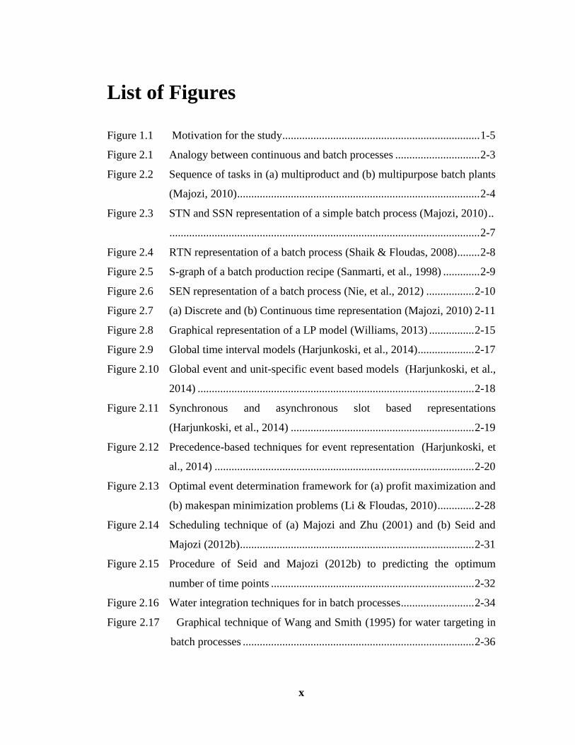
Figure 2.9 Global time interval models (Harjunkoski, et al., 2014)
(b) Global and Unit-specific event- based models
The global event-based technique is a generalization of the global time intervals
technique. Their similarity relies on the fact that the time intervals are common across
all the units. However, in global event based models, each time interval has a variable
length which is not known beforehand as shown in Figure 2.10(a). This implies that
the duration of each interval is modelled as a decision variable during optimization
(Mendez, et al., 2006). The unit specific event based representation, on the other
hand, use a variable time grid which is each processing unit. Its uniqueness comes
from the fact that it allow the value of a time point to vary from one unit to the other
as shown in Figure 2.10(b).
The advantage of global event -based models is the fact that they provide a reference
time grid for all units which usually simplify formulation pertaining to the
optimization of batch plants. However, it usually requires a larger number of event
points compared to unit-specific event based models. In the latter, the use of unit-
specific time grids allow some units processing fewer batches to use fewer time
points which leads to an overall reduction of time points used in a given formulation.

Chapter 2 Literature review
2-18
2'
T4T3
T5 T6
T1 T2
U2
U1
1 2 3 4
(b) Unit-specific event based models
Units
3'
T4T3
T5 T6
T1 T2
U2
U1
1 2 3 4 5
(a) Global event based models
Time
points
Units
5Time
points
Figure 2.10 Global event and unit-specific event based models (Harjunkoski, et
al., 2014)
(c) Slot based models
Slot based models use a predefined number of time slots of unknown duration for
each processing unit in order to allocate them to different tasks to be performed.
These techniques often allow a task to be allocated to more than one slot if the
required number of time slots is overestimated. Slot based representations are very
similar to event based representations in that they both use time grids to represent
tasks and events. They are further subdivided into synchronous (process slots) and
asynchronous (unit slots) models. Synchronous models use common slots across all
units, as shown in Figure 2.11(a) while asynchronous models use different slots for
different units, as illustrated in Figure 2.11(b) (Mendez, et al., 2006). Therefore, due

Chapter 2 Literature review
2-19
to the similarity between slot based and event based models, it can be concluded that
asynchronuous slot based models use fewer time slots and reduce the size of resultant
mathematical formulations.
T4T3
T5 T6
T1 T2
U2
U1
Slot 1 Slot 2 Slot 3 Slot 4
(a) Slot based models (synchronous)
Units
Time
slots
T4T3
T5 T6
T1 T2
U2
U1
Slot 1 Slot 2 Slot 3 Slot 4
Slot 1' Slot 2'
(b) Slot based models (asynchronous)
Units
Time
slots
Figure 2.11 Synchronous and asynchronous slot based representations
(Harjunkoski, et al., 2014)
(d) Precedence- based techniques
Precedence-based techniques are batch oriented formulations aiming to determine the
optimal sequence of jobs in each processing unit present within a batch plant. These
techniques do not use time grids uniques the other aformentioned tecniques. They are
divided into immediate precedence and general precedence based techniques.

Chapter 2 Literature review
2-20
Immediate precedence techniquess only consider the immediate predecessor of a
batch whilst general precedence based techniques consider any predecessor of a
particular batch in a unit. For instance, as shown in Figure 2.12, the immediate
predecessor of task T4 which is performed in unit U1 is task T3 whilst tasks T1, T2
and T3 are all considered as predecessors of task T4 in general precedence based
formulations. General precedence based techniques have the advantage of using a
single sequencing variable to allocate a pair of batch tasks to the same shared
resource such as a processing unit. Therefore, they result in smaller formulations
when compared to immediate precedence based techinques. The major weakness of
precedence based techniquess is the increase in the number of sequencing variables
with increasing number of batches to be scheduled. Consequently, this can result in
very large scale models for real case scenarios (Mendez, et al., 2006).
Immediate precedence
General precedence
T4T3
T5 T6
T1 T2
U2
U1
Units
Figure 2.12 Precedence-based techniques for event representation (Harjunkoski,
et al., 2014)
2.3.4 Review of short-term scheduling models for batch processes
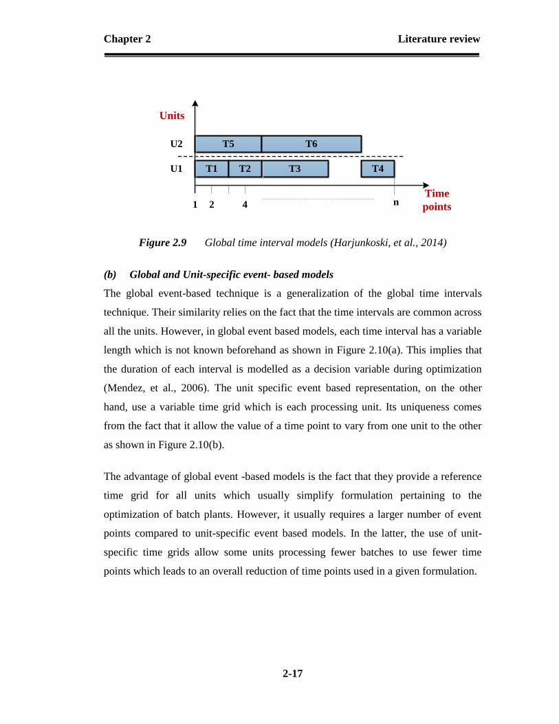
Kondili et al. (1993) developed the earliest model for the short-term scheduling of
multipurpose batch processes. Their model used the STN for recipe representation, a
discrete time representation where a single grid is used for the mapping of tasks in all
Chapter 2 Literature review
2-21
existing units as shown in Figure 2.9. A three-index binary variable Wijt was used to
denote the start of the processing of task i by unit j at the beginning of time period t .
Allocation constraints were used to ensure that a unit only performed one task at a
time while material balances captured the net increase or decrease in inventories in
storage tanks. The formulation allowed all type of intermediate storage policies to
exist within the process. Many other aspects of batch process scheduling were
considered in this formulation as listed below.
The temporary unavailability of resources during certain time periods. This
may be due to the need for maintenance or breakdown during plant operation.
The limited availability of utilities and discrete resources such as manpower.
Sequence-dependent cleaning which entails that the extent of cleaning can
depend on the sequence of tasks in that units.
Frequency-dependent cleaning which considers cases where the need for
cleaning a unit depends on the frequency of its utilization
The model aimed to maximize the profit of the plant and the objective function
considered the production revenue, the cost of feedstocks, the running costs of
storage tanks and the cost of utilities. However, due to the discrete time
representation, the formulation led to very large MILP scheduling problems.
Schilling and Pantelides (1996) then presented a synchronous slot based scheduling
formulation using the RTN framework of Pantelides (1994). The formulation forced
the starting and finishing time of all tasks to coincide with time points on the time
grid. In other words, the length of a time slot was modeled to be equal to the duration
of a specific task. A variable processing time which depends on the size of the batch
was considered for all tasks. The objective of their formulation was to maximize the
net accumulation of resources minus the cost of performing various tasks. The
authors addressed the issue of large integrality gaps in continuous time formulations
which increase their computational burden by developing a branch and bound

Chapter 2 Literature review
2-22
algorithm where both continuous and integer variables are branched and tighter
bounds are imposed on slot durations.
Zhang and Sargent (1996) then developed a global event based models using a RTN
representation to improve the discrete time RTN model of Pantelides (1994). In this
formulation, A batch task was modelled to start at an event time point while
consuming and generating a set of resources at the start and end of its execution
respectively. The formulation aimed to maximize the plant profit and yielded a large
nonconvex MINLP for which the author addressed the computational difficulties
associated with the nature of the model. The model was then simplified by reducing
the number of nonlinear terms and fixing the production recipe, i.e. fixing the
processing time of batch operations. This then resulted in a drastic reduction in model
size and CPU time.
Cerda et al. (1997) developed the first precedence based MILP formulation for the
scheduling of a single stage multiproduct batch plant with parallel units. The concept
of immediate predecessor and successor of a batch was introduced to effectively
handle sequence-dependent changeovers between different batches in a unit. The
formulation aimed to determine the optimum sequence of jobs in processing units.
The model assumed that the size of each batch was fixed to the maximum capacity of
the unit performing the job. Different batches producing the same order were
modeled to be performed in the same unit. The objective functions considered were
the minimization of the overall tardiness, the makespan and the number of tardy
orders.
Ierapetritou and Floudas (1998) introduced the concept of unit specific event-based
modelling to address the problems associated with global event-based and discrete
models. Their MILP formulation adopted a STN for batch recipe representation. A
concept of decoupling task events from unit events was introduced in an effort to
reduce the size and computational burden of previous continuous time formulations.

Chapter 2 Literature review
2-23
The binary variable Wijt commonly used in previous STN formulation led to large
numbers of binary variables of dimension i x j x t. The authors replaced it with two
binary variables wv(i,n) and yv(j,n) where wv(i,n) assigns the beginning of task i to
time point n and yv(j,n) denotes the beginning of the utilization of unit j at time point
n. e allocation constraint was formulated by ensuring that only one task is assigned to
a unit at any given point in time as described by Equation (2.6) below.
NnJjniyvniwvjIi
,,),(),( (2.6)
The authors also demonstrated that for batch processes where a unit is only allowed
to process one task, Equation (2.6) can be reduced to wv(i,n)=yv(i,n). This allows the
elimination of the yv(i,n) binary variable and Constraint (2.6), resulting in a drastic
reduction of the model size. Time sequencing constraints for tasks occurring in the
same and/or different units were also introduced and the events were modelled as
shown in Figure 2.10(b). Moreover, nonlinear terms usually found in previous
continuous time formulations were avoided, rendering the formulation simpler and
easier to solve.
Majozi and Zhu (2001) introduced the SSN representation and presented a scheduling
formulation attempting to improve the existing unit-specific event-based models.
Their formulation only used a binary variable y(s,p) to denote the use of a state s at a
given time point p which inherently implied that the unit is starting to process a
certain task is being processed in a unit at a given point in time. The authors
considered the case where the duration of a task can vary depending on its batch size.
Overall, Their formulation was able to further reduce the number of binary variables
used to model a scheduling problem. Consequently, the computational intensity of
unit specific event based models was alleviated, enabling scheduling problems to be
solved to optimality. An aggregation model was also presented whereby processing
units performing similar tasks in a particular processing stage are modelled as a single

Chapter 2 Literature review
2-24
unit. This was performed to achieve a further reduction in the size of mathematical
models aiming to schedule multi-stage batch plants with an in-phase operation of
processes.
Maravelias and Grossman (2003) presented a global event based formulation for the
scheduling of multipurpose batch plants using a STN framework. The authors
considered both a fixed an a variable processing time of tasks and used the concept of
task decoupling proposed by Ierapetritou and Floudas (1998). Various storage
policies including the UIS, FIS, NIS and ZW policies were explored. A mixed global
event representation was introduced wherein tasks producing at least one unstable
state and requiring a ZW policy were modelled to start and end at interval boundaries.
All other tasks were allowed to end at any time within a given time interval. The
global alignment of events allowed the formulation to have less sequencing
constraints compared to unit specific event-based approaches. The authors also
proposed a hybrid Generalized Disjunctive/Mixed Integer Programming technique to
reduce the CPU time of global event-based models.
Sundaramoorthy and Karimi (2005) proposed a simple synchronous slot based
approach for the short-term scheduling of multipurpose batch plants. The original
three-index binary assignment variable proposed by Kondili et al. (1993) was used
instead of the decoupling method of Ierapetritou and Floudas (1998). The authors
demonstrated that, for a set of unit Ji performing task i, both approaches led to the
same number of binary variables per event point which is equal to the sum of
cardinalities of set Ji for all tasks i. Their formulation allowed tasks to span over
multiples slots by defining a binary variable Yijk and three 0-1 continuous variables
Zjk, yijk and YEijk as follows.
0
1
ijkY (2.7)
Otherwise
if unit j begins task i at time Tk

Chapter 2 Literature review
2-25
0
1
jkZ (2.8)
0
1
ijky (2.9)
0
1
ijkYE (2.10)
Logical constraints where used to ensure that the 0-1 continuous variables behave like
binary variables and model the status of a unit at a specific time point Tk. A slot k was
modelled to have a duration SLk, starting from Tk-1 to Tk. The material balance
consisted of modelling the variation of batch size as materials enter or leave the unit.
Material inventory at each processing stage was ensured by performing a material
balance on storage tanks at each time point by assuming that tasks withdraw and
transfer materials from and to storage at the beginning and end of their operation. The
transfer time was assumed to be included in the processing time as assumed in
previous formulations. Both profit maximisation and makespan minimisation were
considered as objectives of batch production schedule optimisation.
Shaik and Floudas (2008) then first explored the use of RTN representation in unit
specific event-based models. A binary variable w(i,n) was used to assign a given task
i at the beginning of time point n. The formulation consisted of resource balances,
capacity, and sequencing constraints. The authors included sequencing constraints to
adequately cater for the FIS policy as opposed to simply using an upper bound on the
amount of materials stored at each time point. The latter, adopted by the work of
Ierapetritou and Floudas (1998) and Majozi and Zhu (2001), can lead to infeasible
Otherwise
Otherwise
if unit j begins a task at time Tk
Otherwise
if unit j is continuing to perform task i at time Tk
if unit j end task i releases its batch at time Tk

Chapter 2 Literature review
2-26
schedules which violate storage constraints. This is mainly due to the fact that, in unit
specific event based, time points have time values differing from one unit to the
other. The FIS sequencing constraints of Shaik and Floudas (2008) were modelled as
follows.
))1,(),'(2(),'(),'(),'()1,( '' niwniwHnibniwniTniT ii
ss (2.11)
)),'(1(),'(),'(),'()1,( '' niwHnibniwniTniT ii
ss (2.12)
)),'(1(),'(),'(),'(),( '' niwHnibniwniTniT ii
ss (2.13)
Constraints (2.11) and (2.12) together enforced a zero wait policy between two
consecutive tasks i and i’, respectively producing and consuming a resource with
limited intermediate storage. Ts(i,n) denotes the starting time of task i at a given time
point n. In doing so, treating storage as separate tasks was avoided. Constraint (2.13)
then ensures that the starting time of the task consuming an intermediate state with
finite storage should start before the end time of its producing task if both tasks occur
at the same event point n.
Ferrer-Nadal et al. (2008) later addressed the assumption of lumping the transfer time
of intermediate materials between two units into the processing time of tasks involved
in their production. This assumption is usually based on the negligible duration of the
transfer time as compared to the processing time of a task. The authors proposed a
general precedence based model for multistage batch processes which involves
synchronization of processing units during transfer time. This entailed that the units
supplying and receiving intermediate materials could not process any task during the
transfer time in order to obtain a feasible plant schedule. The objective function of the
optimization model was the minimization of the makespan.

Chapter 2 Literature review
2-27
Li and Floudas (2010) addressed the major issue of time point determination
associated with continuous time formulations. They developed a framework to
determine the optimum number of time points for scheduling models aiming to
maximize profit or minimize makespan. Their technique was based on a unit specific
event based model proposed by Shaik and Floudas (2009) which relied on a three
index binary variable w(i,n’,n) defined as follows.
0
1
)n,'n,i(w (2.14)
This allowed a particular task to span over multiple time points between n’ and n. The
model was extended by Li and Floudas (2010) to consider a wider range of storage
philosophies, i.e. UW, ZW, FW, FIS and UIS, and their implication in the time point
determination framework. The proposed determination framework is given in Figure
2.13 where CIS, Nmax , Nmin, and Nopt stand for critical intermediate states, maximum,
minimum and optimum number of event points respectively. A critical intermediate
state (CIS) in this case was defined as the intermediate material that has the highest
effect on the objective value when solving the scheduling model with relaxed
sequencing constraints. An iterative procedure was used to determine the maximum
number of time points Nmax and the CIS(s). The main issue with iterations is the
drastic increase in the time required to get the optimum plant schedule as the size of
the model increases. It is worth pointing out that for a makespan minimization
problem, the framework suggests that a feasible makespan should be determined prior
to the determination of the CIS as shown in Figure 2.13(b). This was obtained by
solving the scheduling model using the minimum number of time points while
restricting the CPU time and ensuring that the product demand was not exceeded.
Task i starts at time point n’ and ends at time point n
Otherwise

Chapter 2 Literature review
2-28
Determination of
CIS (s)
Determination of
Nmax
Determination of
Nmin
Branch and bound
strategy for Nopt
Start
End
Determination of
CIS (s)
Determination of
Nmax
Determination of
Nmin
Branch and bound
strategy for Nopt
Start
End
Feasible makespan
for model
(a) (b)
Figure 2.13 Optimal event determination framework for (a) profit maximization
and (b) makespan minimization problems (Li & Floudas, 2010)
Susarla et al. (2010) proposed an asynchronous slot based model for the scheduling of
multipurpose batch plants. A task was allowed to span consecutive time using a
binary and three 0-1 continuous variables as proposed by Sundaramoorthy and
Karimi (2005). The formulation also catered for non-simultaneous transfer of
materials from storage units to processing units. This was modelled using two
variables δjk and θjk which represent the time period for which a unit j is idle at the
beginning and the end of slot k respectively. Therefore, transfer of materials between
storage tanks and processing units were allowed to occur non-simultaneously within

Chapter 2 Literature review
2-29
periods δjk and θjk respectively. This implied that a start could then start and end
anytime within a slot. The formulation accounted for various storage configurations,
i.e. FIS, UIS, NIS, and different wait policies for intermediate materials, i.e. UW,
FW, and ZW policies. Different possible objective functions were considered for
schedule optimization and this included revenue maximization, makespan
minimization and net profit maximization. The net profit in this formulation took into
account the cost associated with all produced materials rather than just sellable
products.
Seid and Majozi (2012a) then presented a novel technique for the scheduling of
multipurpose batch plants based on an SSN framework. The authors improved on the
formulation of Majozi and Zhu (2001) by reducing the number of time points and
states used to model tasks and events. Their formulation used a state to represent a
task to be processed instead of representing an input or output material as proposed
by Majozi and Zhu (2001). The reduction in the number of time points was achieved
by allowing the starting and finishing time of a task to occur at the boundaries of a
given slot p as opposed to using two distinct time points. The difference between both
models is shown in Figure 2.14. This resulted in a considerable reduction in the
model size as compared to previous formulations. The authors also proposed a
flexible method for handling intermediate materials with FIS constraints through the
use of Constraints (2.15) and (2.16) below.
s
spjin
inj
inj
Jj
U
j
U
s
Ss
in
ju
sp
spsxVQSpsqpsm ,11,1,
,
(2.15)
psxHpsypsyHpstpst in
j
in
j
in
jp
in
ju ,1,,21,, ''
(2.16)
Constraint (2.15) ensures that the amount of intermediate state stored at any point in
time does not exceed the available storage capacity. The binary variable x(s,p)
indicates the availability (x(s,p)=1) or absence of storage (x(s,p)=0) for intermediate
sate s at time slot p. Constraint (2.16) then states that the finishing time of the

Chapter 2 Literature review
2-30
producing task should coincide with the starting time of the task consuming state s
provided that no storage is available for this state, i.e. x(s,p)=0. This constraint is
relaxed if there is an available storage for intermediate state s, i.e. x(s,p)=1. The PIS
policy for materials having a finite intermediate storage capacity was explored. The
unit producing such materials was allowed to be used for its temporary storage
provided that it is not assigned to any other task during that time period.
Seid and Majozi (2012b) then used the scheduling model of Seid and Majozi (2012a)
to develop a novel approach to predict the optimum number of time points. The
proposed approach is shown in Figure 2.15 Their prediction was based on the number
of instances a critical unit is used within a given horizon. This was obtained by
solving the proposed LP max and LP min models which were based on the analysis
of the production recipe. Their methodology did not require iterations at any step of
the time point determination framework as opposed to the work of Li and Floudas
(2010).
Shaik and Vooradi (2013) then presented a novel unit specific event approach for the
unified treatment of all resources aiming to maximize the plant profit. The resources
considered included material states, storage tasks, cooling water, low-pressure steam
(LPS), high-pressure steam (HPS), and discrete resources such as manpower. This
approach unified STN and RTN based formulations with the difference residing in
the way equipment resources are handled. Tasks were allowed to span multiple event
points n using a binary variable w(i,n,n’) as proposed by Shaik and Floudas (2009). A
new feature was introduced whereby the number of events a task is allowed to span
vary from one task to the other. The sttorage of materials were modelled as separate
tasks in order to avoid aggregations of storage tanks and sharing of storage tanks was
considered. The formulation also allowed different tasks using the same utility to
occur at different point in time to improve the global alignment philosophy proposed
by Shaik and Floudas. Satisfaction constraints were used to cater for scheduling
problems with multiple product orders.

Chapter 2 Literature review
2-31
injs out
js in'js out
'js
1p 2p 2p 3p
Tasks
Time
points
(a)
injs in
'js
1p 1p 2p 2p
Tasks
Time
points
(b)
Figure 2.14 Scheduling technique of (a) Majozi and Zhu (2001) and (b) Seid and
Majozi (2012b)
Chapter 2 Literature review
2-32
Step 1: Solve LP max using the maximum number
of time points
Calculate the number of time points required by each
unit- the critical unit requires the maximum number
of time points
Step 2: Solve LP min to minimize the number of
time points required by the critical unit while fixing
the objective value obtained from LP max
Calculate the predicted optimum number of time
points
Step 3: Solve sheduling model using the predicted
number of time points as a root node in a branch and
bound technique
Figure 2.15 Procedure of Seid and Majozi (2012b) to predicting the optimum
number of time points
2.4 Wastewater minimisation in batch plants
The minimisation of freshwater use in batch plants is usually achieved by
implementing process integration opportunities. El-Hawagi (1998) defines process
integration as a “holistic approach to process design and operation which emphasizes
the unity of process units and objectives”. Its merit relies on its ability to integrate
various objectives such as environmental problems (e.g. pollution) with other process

Chapter 2 Literature review
2-33
objectives like profitability and utility reduction. The application of process
integration techniques in batch processes has been the subject of many research
studies. These techniques include direct reuse, indirect reuse, and regeneration reuse.
Direct reuse consists of transferring water between two different units provided the
finishing time of the unit discharging water and starting time of the task receiving
water coincide as shown in Figure 2.16(a). Indirect reuse involves the usage of
storage tanks to allow water to be stored for later reuse. In this case, the time
dimension is relaxed in the sense that the starting and finishing times of water using
operations do not coincide as shown in Figure 2.16(b). Regeneration reuse consists
of partially treating highly contaminated wastewater to facilitate its reuse for further
reduction in freshwater intake. Depending on the operation mode of the regeneration
process, one or two storage tanks can be used as shown in Figure 2.16(c). A single
storage and feeding tank is used for the batch operation of the regenerator while two
or multiple storage tanks are required for continuous or semi-continuous operation of
the regenerator.
Existing research studies for wastewater minimisation in batch processes are broadly
grouped into fixed schedule and flexible schedule techniques. Fixed schedule
techniques consider that the schedule of the plant is known prior to applying any
water integration techniques. Flexible schedule techniques, on the other hand, allow
the scheduling of batch operations to be performed simultaneously with the synthesis
of the batch water network for wastewater minimization. Fixed scheduling techniques
usually simplify the optimization problem to only a water allocation problem while
flexible schedule technique enables a schedule yielding minimum consumption of
freshwater to be obtained. The latter then guarantees more water reuse opportunities
to be found which entails a possibility for more reduction in wastewater generation.

Chapter 2 Literature review
2-34
Task 1
Task 2
1t
Task 1
Task 2
1t
sto
rag
e
2t
Task 1 Task 2
1t
Regeneration
2t
sto
rag
e
sto
rag
e
(a) Direct reuse (b) Indirect reuse
(c) Regeneration reuse
Figure 2.16 Water integration techniques for in batch processes
2.4.1 Fixed schedule techniques
Fixed schedule techniques are classified by the adopted optimisation approach.
Optimisation techniques in place include insight based techniques, mathematical
modelling techniques, and hybrid techniques. Insight based techniques allow the
engineer to visually target minimum freshwater using graphs and/or algebraic
concepts and readily design the resultant integrated water network. However, Their
main limitation is their inability to adequately handle multidimensional optimisation
problems such as wastewater minimisation with flexible schedule and multiple
contaminants. Mathematical modelling techniques involve the development of

Chapter 2 Literature review
2-35
programming models in which minimum freshwater use and network design are
simultaneously yielded by the model. While this approach is not limited in
dimension, computational difficulties such as high CPU time may arise when solving
complex optimization problems. Hybrid techniques then combine both insight-based
concepts and mathematical modelling with the aim of benefiting from both
techniques. Contributions for wastewater minimisation made under each category of
optimization techniques are thoroughly explored in this section.
(a) Insight-based techniques
Wang and Smith (1995) were the first to develop a technique for wastewater
minimisation in batch processes. The authors modified the water pinch technique of
Wang and Smith (1994) to consider time as a primary constraint and concentration
driving force as a secondary constraint. This entailed dividing a specific problem into
concentration intervals and time subintervals, grouping existing processes in each
concentration interval and reusing effluents from one concentration interval to the
subsequent one. Freshwater was fed at intervals were no effluent was available for
reuse and as a top up to meet the water requirement in each concentration intervals.
Figure 2.17 shows graphs of water targeting at two consecutive intervals whereby
freshwater is supplied to processes existing in the first interval and effluents from the
first interval are cascaded to the second interval for reuse. The cascaded water is
represented in Figure 2.17 as “water available for reuse”. Once the targeting
procedure was performed in all existing concentration intervals, the integrated batch
water network was then designed. However, their resultant network could not be
implemented in batch processes for it allowed the reuse of water to occur between
operations with overlapping time intervals. The network also suggested the usage of
storage which was not practically needed because timing constraints were satisfied
for direct reuse to occur. Furthermore, this technique can only be applied to mass
transfer based operations, i.e. operations where water is used as a lean stream for the
extraction and removal of contaminants.

Chapter 2 Literature review
2-36
1t 2t 3t
1G
Amount of
water
Time
Water available
for reuse
Composite
curve
Pinch
point
2G
3G
4G
Concentration interval 2
1t 2t 3t
1G
Amount of
water
Time
Composite
curve
2G
3G
Concentration interval 10 1c
Fre
shw
ate
r
1c 2c
Figure 2.17 Graphical technique of Wang and Smith (1995) for water targeting in
batch processes
Foo et al. (2005) proposed a numerical procedure for the synthesis of maximum water
recovery network for batch processes with a single key contaminant. The technique
involved two stages whereby the first stage consisted of determining the minimum
freshwater and wastewater targets using the time-dependent water cascade analysis
(WCA). The second stage then focused on designing the water network based on the
targeted utility consumption. Their work was adapted from the two-stage procedure
of Foo et al. (2004; 2005a) for the synthesis of batch mass exchange networks and the
WCA technique of Manan et al. (2004) targeting minimum freshwater flowrate in
continuous processes. This technique employed classification of a process into a
source and/or demand introduced by Dhole et al. (1996) to allow for different types of
processes to be included while developing strategies for the optimization of water
use. This enables WCA to cater for both mass-transfer and non-mass transfer based
operations in both batch and semi-continuous processes.

Chapter 2 Literature review
2-37
The time-dependent WCA technique is performed in a tabular form and can be briefly
explained as follows. In the first column, all existing contaminant concentration
levels expressed in ppm are arranged in ascending order. In the next column, the
existing concentration levels are expressed in terms of water purity with freshwater
being set at a concentration of one million ppm. Next, all sources and demands are
tabulated at their corresponding purity level and within the time interval in which
they exist. The WCA of Manan et al. (2004) is then performed at each time interval to
obtain the minimum freshwater and wastewater target by exploring direct reuse of
water. The minimum freshwater and wastewater targets across all intervals add up to
the optimum freshwater use and wastewater generation of a given batch process.
When indirect reuse is explored, the targeting is performed once by adding sources
and demands at each purity level across time intervals. However, mixing of sources
of different purities in the same storage tank is not allowed and this can lead to a large
number of storage tanks when many sources of different qualities require storage.
Majozi et al. (2006) address the drawbacks of Wang and Smith (1995) formulation by
presenting a new graphical technique for wastewater minimisation in batch processes.
The technique considered cases where time and concentration are interchangeably
treated as primary constraints as shown in Figure 2.18. When time is treated as a
primary constraint, a plot of water demand versus time is used to find possible reuse
opportunities across concentration intervals. This is illustrated in Figure 2.18(a),
where water demand profile and available water cascade from previous concentration
intervals are represented. Figure 2.18(b) then shows a graph of concentration versus
water demand where processes are represented using diagonal lines with reuse of
water only allowed between completed and starting operations. The technique also
considered the use of dedicated storage vessels and processing units as potential
storage tanks to override time and increase water reuse opportunities in both state
operations. Both single and cyclic batch operations were addressed in this
formulation. However, this technique was limited to mass transfer operations.

Chapter 2 Literature review
2-38
1t 2t 3t 4t 5t
1D
2D
3D
4D
5D
6D
Time
Water
demand
Available
water
profile
Water
demand
profile
(a) Time - primary constraint
Concentration interval1C 2C
Operation 1
(Complete)
Operation 2
(Active)
Operation 3
(Active)
Water transfer
1D 2D 3D
1C
2C
3C
Time interval
1t 2t
(b) Concentration - primary constraint
Water
demand
Con
cen
trati
on
Figure 2.18 Graphical techniques of Majozi et al. (2006) with (a) time and (b)
concentrations treated as primary constraints.

Chapter 2 Literature review
2-39
Liu et al. (2007) then presented a concentration interval analysis (CIA) technique for
the synthesis of water utilization network in discontinuous processes. The algebraic
technique consisted of constructing a time-dependent concentration interval table
where time intervals were defined as the duration of different operations while certain
operations could occur at different intervals. Similar to the time-dependent WCA, the
minimum water usage was first determined for each time interval and then effluents
from one interval were reused in the subsequent interval using a storage vessel to
override time. The network design was performed after the water targeting procedure
and the resultant network was compared to the one obtained by Wang and Smith
(1995) for the same plant. Although the formulation provided a better network in
terms of the number of storage tank used, it had the limitation of being more suitable
for semi-continuous processes rather than truly batch processes.
Chen and Lee (2008) presented a graphical technique for the design and synthesis of
a batch water network involving different types of water using operations. A quantity-
time graphical representation was introduced in this formulation as shown in Figure
2.19. This representation clearly maps all water sources and demands available within
a batch plant which then allowed for the optimum utility consumption and network
structure to be determined simultaneously. The technique also adopted the source-
demand representation to cater for mass transfer and non-mass transfer based
operations in both batch and semi-batch operation modes. The utility targeting and
network design were achieved by first identifying all possible water reuse and
recycling opportunities with a minimum number of storage tanks that lead to a
practically feasible water network configuration. Similar to the work of Foo et al.
(2005), this technique did not allow the mixture of different water sources with
different contaminant levels in one storage tank. Moreover, the technique considered
both single and cyclic batch operation.

Chapter 2 Literature review
2-40
Quantity
(of water)
Time
D1
D3
(C1)
S1
D4
(C2)
S3S2
D2
Water reused
From S1 to D4
DFWAmount of
freshwater
required
to satisfy D4
-Q1
-Q2
Q3
Q4
Q5
t1 t2 t3 t4 t5 t6 t7
Figure 2.19 Graphical technique of Chen and Lee (2008)
Chaturvedi and Bandyopadhyay (2012) proposed an algebraic methodology for
wastewater minimisation in both batch and semi-continuous processes. The
formulation considered fixed flowrate operations with a single contaminant and
known starting and finishing time. The targeting procedure started by considering a
single batch process with two time intervals. Next, a three-time intervals batch
process was integrated leading to a targeting technique for a batch process with N
intervals. Using a set of mathematical concepts, a targeting algorithm for both single
and cycling batch was established. For a single batch, the procedure consisted of
firstly dividing the time horizon into time intervals such that their boundaries
coincide with sources and/or demands. The integration was performed in the first
interval to achieve minimum waste generation and effluents from the first interval
were then used as a source in the next interval. The procedure was carried on to the
last time interval. For cyclic batch, the targeting procedure was performed

Chapter 2 Literature review
2-41
irrespective of the sequence of intervals by using a continuous process approach. The
authors later extended the formulation to batch processes with multiple freshwater
sources having different qualities (Chaturvedi & Bandyopadhyay, 2013).
(b) Mathematical modelling techniques
The work of Almato et al. (1999) is among the earliest efforts made toward the
development of a mathematical technique for the optimization of water use in batch
processes with a fixed production schedule. The NLP formulation consisted of
synthesizing a water network with minimum cost using a stream- tank assignment
method. The superstructure was made of a set of storage tanks in place to facilitate
indirect reuse of effluents from one unit to the other. The optimization problem then
consisted of finding the optimum interconnections between units performing batch
tasks and storage tanks while determining the quantity and quality of water carried by
each pipe. The objective function accounted for freshwater cost, the cost of hot and
cold utilities needed to reach the targeted temperature of water streams, and the costs
associated with piping and storage.
Kim and Smith (2004) then presented a mathematical formulation for minimization
of water use by discontinuous processes. The technique explored both direct and
indirect water reuse within a plant. The authors adopted the concept developed by
Wang and Smith (1995) which entails splitting an interval at which a task occurs into
subinterval to allows more water reuse opportunities to be found. However, by the
definition of a batch process operation, materials can only be fed to or discharged
from a unit at the beginning or the end of a specific process. Hence this formulated
was more suited for semi-continuous processes The objective function consists of the
minimization of annualized cost of the water network which includes the cost of
freshwater, cost of storage and the piping and interconnection costs. Majozi (2005a)
proposed an MILP formulation for wastewater minimization in multipurpose batch
plants which considered a single key contaminant. Minimum water usage was
Chapter 2 Literature review
2-42
achieved by fixing the contaminant concentration of outlet streams from each unit to
its maximum allowable value and searching direct reuse and recycle opportunities
between operations.
Chang and Li (2006) designed a water equalization system of buffer tanks in order to
achieve the desired flow and concentration of wastewater streams entering the
wastewater treatment system. The formulation used a discrete time representation to
map operations with predefined starting and finishing time. The number and type of
treatments units were stated to be dependent on the type and number of contaminants
present in the wastewater streams. However, no information related to the type of
treatments units were given for the presented case studies. Furthermore, batch
operations were only modelled as sources of wastewater and no reuse was explored.
Li and Chang (2006) extended this formulation to consider the use of buffer tanks to
facilitate indirect reuse of water by modelling batch operations as both wastewater
sources and sinks. Liu et al. (2009) considered the use of a central regenerator for
highly contaminated wastewater treatment as an extension of the work of Li and
Chang (2006).
Lee et al. (2013) presented a mathematical technique to integrate batch and
continuous processes through the use of storage vessels based on a continuous time
approach. Lee et al. (2014) then proposed a four-step mathematical procedure for the
minimization of freshwater, storage capacity as well as interconnections between
units in a water allocation network (WAN) involving both mass transfer and non-
mass transfer based operations.
(c) Hybrid techniques
Oliver et al. (2008) presented a hybrid technique for the synthesis of water reuse
network in batch processes. It consisted of a combination of water pinch analysis and
mathematical modelling to optimize water utilization in a winery located in Suan

Chapter 2 Literature review
2-43
Juan, Argentina. The plant consisted of 30 water using operations with 25 of them
being washing operations. Hence, the formulation focused on mass transfer
operations. The possibilities for water reuse were first identified using a water pinch
technique and the minimum freshwater consumption was obtained. The resultant
water network from the pinch analysis required a very large number of storage units
to override the time dimension due to the continuous approach employed. A
mathematical model was then constructed to provide a cost-effective water reuse
network while using the minimum freshwater use obtained from the graphical
technique as a lower bound. The model was based on a predefined schedule.
However, the mass balance constraints involved in the mathematical model where
suitable for semi-continuous processes resulting in a technique that cannot be applied
to batch processes.
Foo (2010) developed a MILP formulation for the synthesis of a batch water network
with a predefined schedule based on insight concepts of the time-dependent water
cascade analysis. Similarly to conventional insight based technique, the technique
allowed the minimum freshwater consumption and wastewater generation to be
determined prior to the design of the water network. In addition to direct reuse within
a time interval and indirect reuse across intervals, regeneration reuse was explored
through the use of a wastewater treatment unit. The treatment unit was modelled
using a black-box approach with fixed outlet concentration. Both two-step and single
step optimisation were used whereby the former was employed to sequentially
minimize freshwater use and storage capacity without considering costs. The latter
was then used to minimise the total annualized cost of the water network by taking
into account the annual freshwater cost, wastewater treatment costs, effluent
treatment cost, the capital cost of storage tanks, and the regeneration cost. The cost of
regeneration was modelled linearly as a function of the total quantity of water fed into
the regenerator. This technique has the advantage including economic aspects such as

Chapter 2 Literature review
2-44
cost in the water targeting procedure as opposed to conventional insight based
techniques.
2.4.2 Variable schedule techniques
Existing wastewater minimisation techniques that consider a flexible schedule are
based on mathematical optimisation due to their complexity. There are no insight-
based techniques that have yet been developed to account for scheduling while
targeting minimum freshwater use in batch processes. However, a recent effort was
made towards the development of a hybrid optimisation technique integrating
graphical targeting and mathematical optimisation in wastewater minimisation
problems. The aim of the hybridisation is to reduce the complexity of variable
scheduling techniques for wastewater minimisation and ease their solution
procedures. This section gives a review of existing mathematical and hybrid
techniques for the minimisation of wastewater in batch processes with the
consideration of a variable schedule.
(a) Mathematical models
Methodologies for freshwater minimisation in batch processes relying on flexible
scheduling frameworks arose in the recent decades. The work of Majozi (2005b) was
first to consider the simultaneous optimisation of the scheduling and water use in
batch processes with a single contaminant. This work was then extended to include
both direct and indirect reuse/recycle as wastewater minimisation techniques. Four
scenarios were explored in the extended formulation, i.e. fixed outlet concentration
and fixed water requirement with and without the presence of water reusable storage.
Although the formulation was applied to batch processes with fixed schedules, the
formulation was opened to flexibility in scheduling as to increase water reuse
opportunities.

Chapter 2 Literature review
2-45
Cheng and Chang (2007) then presented an effective procedure for the optimal design
of a fully integrated water network where batch schedule, water reuse, and
wastewater treatment subsystems were optimised simultaneously. The formulation
was aimed at determining the optimum production schedule, the optimum number,
and size of buffer tanks and the configuration of the pipeline network. The production
schedule was modelled using the STN recipe presentation and the discrete time
representation. By sequentially integrating different subsystems, the formulation
showed the benefits of simultaneously optimising an integrated schedule and water
network through various case studies. The water treatment network consisted of
regenerators with either continuous or batch operation mode modelled using a black-
box approach with fixed removal ratio, pollutant index, and flowrate limits. The
regenerated water was directly disposed to environmental water sinks without
exploring any opportunity for reuse within the plant.
Zhou et al. (2009) presented a two-stage model for the sequential optimisation of
batch schedule and water network system embedding a regeneration process. The
authors attempted to improve on the work presented by Cheng and Chang (2007) by
using continuous time approach to address the limitations of discrete time approach.
The regenerator was intended to treat highly contaminated wastewater to facilitate its
reuse within the process and meet environmental standards for wastewater disposal.
The treatment unit was modelled as a black-box where a contaminant removal ratio
was used to determine the outlet concentration of the purified water and the
percentage of water loss during regeneration was fixed.
Majozi and Gouws (2009) developed a continuous time formulation that
simultaneously optimised batch schedule and multi-contaminant water network.
Direct and indirect reuse were used as wastewater minimisation techniques but
regeneration reuse was not addressed. Li et al. (2010) proposed a mathematical
technique to integrate the scheduling framework and WAN of batch processes using a
state-time-space (STS) superstructure. A combination of both discrete and continuous

Chapter 2 Literature review
2-46
time formulations was used to represent batch schedule based the work of Ierapetritou
and Floudas (1998). Chen et al. (2011) presented an RTN based technique targeting
maximum plant profit by simultaneously optimising the production schedule and
WAN. The formulation considered multiple freshwater sources while exploring direct
and indirect reuse of water between units.
Adekola and Majozi (2011) later extended the formulation of Majozi and Gouws
(2009) by developing a mathematical modelling technique that considered
simultaneous optimisation of batch schedule and multi-contaminant water network
that included central water storage and central regeneration unit. However, the
regeneration unit was modelled as a black box with a predefined removal ratio for
each contaminant and the cost of regeneration was not accounted for in the objective
function.
Chaturvedi and Bandyopadhyay (2014a) presented a two-step procedure to optimise a
water network with multiple freshwater resources using a flexible scheduling
platform. The scheduling model was first solved to obtain the maximum throughput.
Next, the water network was optimised while maintaining the throughput at its
maximum value. The authors then proposed a dual-objective MILP to optimise a
batch water network using a flexible scheduling platform. The first objective function
aimed to maximise the production while the second objective consisted of minimising
freshwater requirement. The formulation made use of Pareto optimal front to capture
the tradeoff between the two objective functions (Chaturvedi & Bandyopadhyay,
2014b).
Adekola and Majozi (2017) recently explored wastewater minimisation in batch
plants by adequately selecting the sequence of tasks occurring in a multipurpose unit.
Their technique was based on the concept of sequence-dependent changeover
operations in which the amount of water required to wash a particular unit after
processing a task depends on the succeeding task.

Chapter 2 Literature review
2-47
(b) Hybrids techniques
Chaturvedi et al. (2016) recently proposed a hybrid technique using both insight
based concepts and mathematical modelling to synthesize a cost-effective batch water
network with multiple freshwater resources. Scheduling in their context was made
flexible by allowing water sources and demand to be shifted while maintaining
production requirements. The formulation claimed that the change in the overall
operating cost of a water network does not depend on the number of the available
freshwater resources. This was proved by integrating the algebraic algorithm
proposed by Chatuverdi and Bandyopadhyay (2012) and mathematical formulations
of Chaturvedi and Bandyopadhyay (2014a; 2014b). Therefore the schedule obtained
for a batch water network with a single freshwater source was fixed when the
problem was extended to multiple resources, thus reducing the model size and
computational intensity.
2.5 Consideration of regeneration
The concept of regeneration reuse in batch processes has been considered in the
published literature. The work of Liu et al. (2009), Zhou et al. (2009) and Adekola
and Majozi (2011) have all explored regeneration reuse as part of the wastewater
minimization as discussed in the previous section. However, a black-box approach
was used to model the performance of the regenerator in the aforementioned
techniques. The main drawback of black-box approaches is their inability to optimize
for the energy consumption of regeneration units. The regeneration of wastewater
involves the use of wastewater treatment technologies. The type of technology
employed strongly depends on the quality of effluents generated and the nature of
contaminants to be removed. Membrane systems evolved as effective ways of
purifying wastewater and are currently found in many wastewater treatment facilities
(Atasi, 2015). However, these technologies require an intensive amount of energy to
considerably reduce the contaminant level in wastewater effluents. This highlights

Chapter 2 Literature review
2-48
the importance of optimising the consumption of energy in membrane systems while
exploring regeneration reuse. This section will give an overview of different
membrane technologies used in wastewater reuse and elaborate further on the
electrodialysis process, the technology of focus in this work.
2.5.1 Membrane technologies for wastewater treatment
Membrane systems are technologies developed for the removal of species in the
aqueous phase by physical or physicochemical mechanisms using a membrane
material (Judd & Jefferson, 2003). A membrane material is a thin film which
separates two phases by selectively allowing the transport of matters as shown in
Figure 2.20(a). The principle of a membrane operation is illustrated in Figure 2.20(b).
A feed stream entering a membrane separation is divided into a permeate, the stream
containing the materials which have passed through the membrane, and the retentate,
which is made of all the non-permeable materials (Mallevialle, et al., 1996).
Membrane processes are becoming popular for bulk water and wastewater treatment
due to the following advantages that they offer over conventional water treatment
techniques (Judd & Jefferson, 2003).
Less energy consumption due to the inexistence of a phase change.
The build-up on membrane surfaces are minimal. This can guarantee a smooth
continuous operation of the treatment process
Little or no addition of chemicals is usually required during separation.
High selectivity
Production of high quality treated effluents

Chapter 2 Literature review
2-49
Feed
Permeate
RetentateMembrane
(a)
(b)
Figure 2.20 Principle of a membrane operation
There is a wide range of membrane operations that can be used for the treatment of
industrial wastewater. They can be classified based on the driving force, the
mechanism of separation, the structure of the membrane and the phases in contact as
presented in Table 2.1. The driving force is the criteria commonly used to
characterize membrane operations. In this regards, Pressure, activity and electrical
potential driven operations are the three main types of membrane operations.
Microfiltration (MF), ultrafiltration (UF), nanofiltration (NF) and reverse osmosis
(RO) are all operations in which the pressure difference across the membrane drives
the separation process in which the solvent is transferred through the membranes. On
Chapter 2 Literature review
2-50
the other, Pervaporation (PV), membrane distillation (MD), membrane stripping
(MS) operate based on the activity difference across the membrane which causes the
membrane to selectively allow the transport of the solvent. Dialysis (DIA) is also an
activity driven membrane in which, unlike the other three aforementioned activity
driven membrane, the concentration difference allows the transport of solutes through
the membrane. Electrodialysis (ED) is membrane operation in which the potential
difference causes ions to selectively pass through the membranes.
Table 2.1 Classification of membrane operations (Mallevialle, et al., 1996)
Membrane
operation
Driving force Mechanism of
separation
Membrane
structure
Phase
1 2
Microfiltration Pressure Sieve Macroscopic L L
Ultrafiltration Pressure Sieve Mesopores L L
Nanofiltration Pressure Sieve+(solution/diffusio
n+eclusion)
Micropores L L
Reverse osmosis Pressure Solution/diffusion+excl
usion
Dense L L
Pervaporation Activity (Partial
pressure)
Solution-diffusion Dense L G
Membrane
stripping
Activity (Partial
pressure)
Evaporation Macropores
(gaz
membrane)
L G
Membrane
distillation
Activity
(temperature)
Evaporation Macropores
(gaz
membrane)
L L
Dialysis Activity
(concentration)
Diffusion Mesopores L L
Electrodialysis Electrical
potential
Ion exchange Ion exchange L L
The membrane structure and the mechanism of separation are key indicators of the
type of contaminant a membrane operation can remove during the treatment of
wastewater. MF and UF are both suitable for the removal of solid particles from
water through sieving. The difference in membrane pore size makes UF capable of
removing smaller particles as compared to MF. NF, on the other hand, is mainly
suitable for the removal of multivalent ions such as calcium and magnesium. RO has

Chapter 2 Literature review
2-51
a dense membrane structure which is tailored to retain salts and low molecular weight
solutes. PV and MS can be used for the removal of volatile organic compounds. MD
can also be applied for the removal of salts in wastewater. DIA selectively allows
ions and low molecular weight solutes to pass through the membrane while rejecting
larger colloidal and high molecular weight solutes. ED is mainly designed for the
removal of ionic species such as salts, acids, and nitrate from wastewater.
This research focused on implementing an ED treatment unit to facilitate the
purification of wastewater generated from batch water network. The main purpose
this implementation is to demonstrate the benefits of embedding a design model of a
wastewater treatment unit while synthesizing a batch water network. It is worth
mentioning that any other membrane operation can be used in this work depending on
the type of contaminants found in wastewater generated from a given plant. A
detailed analysis of the operation and design of the ED system is given in this section.
2.5.2 Electrodialysis technology
(a) Basic concepts
Electrodialysis (ED) is a membrane separation process which is based on the electro-
migration of ions through perm-selective membranes (Tsiakis & Papageorgiou,
2005). In the ED stack, a series of cation- and anion-exchange membranes are
alternatively arranged between a cathode and anode to form dilute and concentrated
cells. The applied direct current (DC) establishes an electric field between the cathode
and the anode. When an ionic solution is pumped through the cells, the electric field
causes the migration of cations and anions towards the cathode and anode
respectively, The positively charged ions pass through the negatively charged cation-
exchange membranes (CEMs) but are retained by the anion-exchange membranes
(AEMs). Likewise, the anions pass through the positively charged AEMs and are
retained by the CEMs. Therefore, there is an increase of ions in one compartment and
ion depletion in the other. This results in the formation of the diluate (depleted

Chapter 2 Literature review
2-52
solution), and the brine (concentrated solution). An ED stack consists of a series of
cell pairs, and a single cell pair contains a CEM, AEM, a diluate and a concentrate
compartment (Rohman & Aziz, 2011; Strathmann, 2004). The schematic
representation of the ED stack is shown in Figure 2.21. Depending on the degree of
desalination required in a plant, multiple ED stacks can be placed in series in order to
achieve a higher contaminant removal.
-
-
-
-
-
-
-
-
-
-
-
+
+
+
+
+
+
+
+
+
+
+
-
-
-
-
-
-
-
-
-
-
-
+
+
+
+
+
+
+
+
+
+
+
-
-
-
-
-
-
-
-
-
-
-
+
+
+
+
+
+
+
+
+
+
+
+ -
+
-
+
+
+
+
+
+
+
+
+
-
-
-
-
-
-
-
-
-
+
+
-
-
CEM CEM CEMAEM AEM AEM
Cell pair
Feed solution
Concentrate
Diluate
Figure 2.21 Schematic diagram illustrating the principle of ED desalination stack
containing CEMs and AEMs in alternating series (Strathmann, 2004).
(b) Advantages and limitations of Electrodialysis
There are quite well-established technologies for the selective removal of salts from
aqueous solutions. These technologies are generally used in industrial applications
where salts are final products or limit further purification of the final products.
However, these technologies are of little use in low-value applications such as
wastewater treatment (Silva, et al., 2013). Membrane processes competing directly
with ED in water desalination applications are reverse osmosis (RO) and recently
nanofiltration (NF). ED has proven to be advantageous over RO and NF in
applications with medium plant capacity of 100 to 20 000 cubic meters per day with

Chapter 2 Literature review
2-53
wastewater or brackish water salinity ranging from 100 to 5000 milligrams per liter
of total dissolved solids. However, RO has proven to be economically viable in large-
scale plants with higher salts concentration. This is due to the fact that, in ED, energy
consumption and the required membrane area are directly proportional to the salt
concentration of the water fed to the process. Nevertheless, ED has also been used for
the treatment of well water of a total salt concentration of about 36 000 milligrams
per liter (Strathmann, 2004).
The advantages of ED over RO, NF and other pressure-driven membrane processes
include, among others, self-cleaning of membranes over a long-term operation,
tolerance of elevated temperature, less raw material pretreatment and easy start-up
and shut-down procedure for processes with intermittent operations (Strathmann,
2004; Silva, et al., 2013). Therefore ED has gained more interest in various
applications such as brackish water desalination (Ortiz, et al., 2005), treatment of RO
concentrate (Zhang, et al., 2012), wastewater minimization (Silva, et al., 2013).
(c) Design and optimisation of an electrodialysis process
The design of an ED unit takes into account the actual ED stack, power supply and
several other components such as pumps, process control devices and feed solution
pretreatment equipment. Different operation modes can be adopted in the design of
ED process. This includes batch mode, continuous mode, and feed-and-bleed mode
with partial recycling of diluate and concentrate streams. The choice of ED operation
mode depends on the degree of desalination required and the feed stream composition
(Mintz & Shaffer, 1980; Strathmann, 2004).
The design and optimization of ED process have been on the research agenda for
years. Korngold (1982) conducted an experimental optimization of an industrial ED
unit to determine the effect of some of the several basic design parameters on the
energy requirement. Lee et al. (2002) then presented a mathematical model for the

Chapter 2 Literature review
2-54
design and optimization of an electrodialysis process for brackish water desalination
in order to evaluate its performance at the design level. The authors gave a detailed
derivation of design equations and experimental methods for the determination of
design parameters. The objective of the formulation was to minimize total costs of the
desalination process which was the sum of capital and operating costs. An iterative
procedure was adopted in the solution procedure of the design model. Tsiakis and
Papageorgiou (2005), improved on earlier work by presenting a MINLP model for
the design and optimization of ED process. A multistage feed and bleed model for
ED operation was introduced and an adequate solution approach was adopted.
2.6 Solution approaches to wastewater minimisation
problems
Optimisation approaches for wastewater minimisation in batch plants involve either
graphical, algebraic or mathematical modelling concepts. Graphical and algebraic
techniques are readily solved by the modeller using graphs and algebraic algorithms
as discussed in the previous sections. Mathematical models for wastewater
minimization, on the other hand, are usually MINLP problems which are solved using
complex algorithms. Some optimisation solvers for mathematical programming are
built in commercial optimization packages to ease the solution process. This section
thus discusses the issue of convexity in mathematical programming, which is a
concept on which solution algorithms are based. The various solutions techniques and
existing optimization solvers for MINLP models are also presented.
2.6.1 Convexity in mathematical programming
Nonlinear programming models are divided into convex and non-convex models.
Convexity in mathematical programming allows the modeller to predict whether a
single optimum value exists or global and multiple other local optimum values are
found in the search space of a specific problem (Edgar & Himmelblau, 1988). A

Chapter 2 Literature review
2-55
convex programming model involves a convex objective function to be minimized or
maximized over a convex region. A convex region is defined as an optimization
search space where a straight segment joining two points in the region lies within that
region. The opposite holds for non-convex regions as shown in Figure 2.22.
xa
xb
Convex
regionxa
xb
Nonconvex
region
Figure 2.22 Convex and Non-convex regions (Edgar & Himmelblau, 1988)
A function is said to be convex when all the infinite set of points satisfying the
function forms a convex region (Williams, 2013). A condition for any function, f, to
be called convex over a region R is presented by constraint (2.17).
)x(f)()x(fx)(x[f baba 11 (2.17)
Rx,x ba
Where θ is a scalar that can take any value between 0 and 1 and xa and xb are any two
distinct values of x. It is worth pointing out that the condition for f to be classified as
a concave function is similar to constraint (2.12). The only differences are the
omission of the negative sign and replace the replacement of the “greater or equal to”
(≤) symbol by the “less or equal to” (≥) symbol in the above inequality (Edgar &
Himmelblau, 1988). This implies that convex function has a single minimum point
while a concave function has a maximum point as shown in Figure 2.23.

Chapter 2 Literature review
2-56
xa xb
x
f(x)
xa xb
f(x)
(b) Convex function(a) Concave function
Figure 2.23 Comparison between (a) Concave and (b) Convex functions (Edgar &
Himmelblau, 1988)
A nonconvex function, on the other hand, exhibits a different behavior as graphically
represented in Figure 2.24. It shows the existence of multiples optimum points among
which are global optimum points such as points d and e. For this reason, nonconvex
problems are difficult to solve compared to convex programming problems.
Therefore, complex algorithms are required to guarantee a globally optimal solution
to a nonconvex problem (Williams, 2013).

Chapter 2 Literature review
2-57
a
b
c
d
e
a- local maximum
b-local minimum
c-local maximum
d-global minimum
e-global maximum
x
f(x)
Figure 2.24 A graphical representation of a nonconvex function (Edgar &
Himmelblau, 1988)
2.6.2 Convexification techniques
MINLP solutions algorithms discussed in the previous section were initially
developed for convex problems. Although the algorithms can be applied to non-
convex models, difficulties could arise when solving MILP master problems and NLP
subproblems. MILP master solutions may not provide valid lower bound while NLP
subproblems suffer the possibility of having multiples local optimum values
(Grossmann, 2002). There exist many ways of circumventing these problems and
among them include linearization and reformulations techniques. These methods are
broadly referred to as convexification techniques and will be briefly discussed in this
section.
(a) Glover transformation
Glover transformation (Glover, 1975) is an exact linearization technique which
eliminates nonlinear terms by replacing them with a set of linear constraints. This
technique deals with a case where polynomial functions contain bilinear terms xy in

Chapter 2 Literature review
2-58
which a continuous variable x is multiplied with a binary variable y. The
transformation is performed as follows:
A new continuous variable r is introduced such that
r replace xy (2.18)
It is assumed that lower and upper bounds of variable x are given as shown in
constraint (2.19). Additional constraints ensuring that z takes the appropriate values
are then constructed as shown by constraints (2.20) and (2.21).
LU xxx (2.19)
yxryx UL (2.20)
yxxryxx LU 11 (2.21)
Constraint (2.20) is obtained by multiplying constraint (2.19) by y to apply bounding
conditions of variable x to variable r. On the other hand, constraint (2.21) equates r to
x when the binary variable y takes a value of 1. Therefore, the Glover transformation
of the bilinear term xy is given by constraints (2.19)- (2.21).
(b) McCormick over- and under-estimators
McCormick (1976) proposed a methodology to obtain global solutions of nonconvex
nonlinear programming problems. It involves the generation of convex and concave
envelopes for factorable functions with bilinear terms. This can be applied to solution
algorithms of nonconvex MINLPs to provide tight convex relaxations, hence
decreasing computational difficulties. The procedure for obtaining convex
underestimators and concave overestimators of bilinear terms can be summarized as
follows.
Chapter 2 Literature review
2-59
Given a polynomial consisting of bilinear terms xy in which x and y are continuous
variables, a new continuous variable m is introduced to replace xy in the function as
shown in constraint (2.22) below.
xym (2.22)
Variables x and y are each provided with lower and upper bounds and this is shown in
constraints (2.23) and (2.24)
LU xxx (2.23)
LU yyy (2.24)
Constraints (2.23) and (2.24) are then decomposed and rearranged to form constraints
(2.25)-(2.28) below.
0 xxU (2.25)
0 Lxx (2.26)
0 yyU (2.27)
0 Lyy (2.28)
By multiplying Constraint (2.25) with (2.27) and replacing xy by m, the following
constraint is obtained.
UUUU yxyxxym (2.29)
Similarly, multiplications of the set of constraints ((2.26);(2.28)), ((2.25);(2.28)) and
((2.26);(2.27)) lead to Constraints (2.30)-(2.32) below.

Chapter 2 Literature review
2-60
LLLL yxyxxym (2.30)
LUUL yxyxxym (2.31)
ULLU yxyxxym (2.32)
Therefore, the underestimators of function xy are represented by constraints (2.29)
and (2.30) while the overestimators are given by Constraints (2.31) and (2.32). This is
graphically illustrated by Figure 2.25.
yU
yL
y
xLxUx
Function xy
Convex underestimators
Concave overestimators
Figure 2.25 Graphical representation of McCormick (1976) envelopes

Chapter 2 Literature review
2-61
(c) Reformulation framework of Lundell et al. (2013)
Lundell et al. (2013) formulated a global optimization framework that implements α-
BB underestimators in the signomial global optimization (SGO) algorithm. They
aimed to provide a general algorithm for all twice differentiable functions of
nonconvex MINLP problems. The SGO technique was developed throughout the
years starting from the work of Porn et al. (1999) to the contribution of Lundell and
Westerlund (2012). It employs single-variable exponential or power transformations
to convexify nonconvex signomial functions. A signomial function is a mathematical
expression made up of signomial terms, i.e. products of power functions. An explicit
mathematical expression of a signomial function of N variables and J signomial terms
is as follows:
J
j
N
i
pjiij xc)x(
1 1
(2.33)
Where cj and pji are real-valued parameters. Special types of signomial functions
commonly found in mathematical programming models are polynomial functions
with bilinear and trilinear terms. Piecewise Linear Functions (PLFs) are used in the
SGO algorithm to capture the relationship between transformation and original
variables which then provide an overestimation of the nonconvex feasible region. A
global solution is found by iteratively updating the PFLs, i.e. iteratively adding
breakpoints to the PLFs, until the solution to the overestimated problem converges.
The α-BB method, on the other hand, is used to obtain convex underestimator of
nonconvex functions. It was first introduced by Liu and Floudas (1993) and Maranas
and Floudas (1995). The underestimation is achieved by adding a quadratic function
to the original nonconvex function in order to suppress any nonconvexity as shown in
Constraint (2.34).

Chapter 2 Literature review
2-62
xgxxxxxg iiii
N
i
i 1
, iii x,xx (2.34)
The value of parameter α in Constraint (2.34) determines the tightness of the α-BB
underestimator and the ideal case is to choose the smallest α value. Figure 2.26 gives
an illustration of the convex underestimation of a one-dimensional sinusoidal
function where the x-domain is partitioned into two intervals. The underestimation is
carried out at each interval and α-values are specified for each interval. In general, the
tightest α-value for the underestimation of a unidimensional function, i.e. i=1, can be
found by taking the second derivative of the left-hand side of Constraint (2.34) and
satisfying the condition given by Constraint (2.35). However, α values for multi-
dimensional functions are obtained using different techniques as proposed by
Adjiman et al. (1997).
xg 2
1 , x,xx (2.35)
g(x)
x
α =c1
α =c2
x1 x2
α -BB underestimators
g(x)
Figure 2.26 α-BB underestimation of a typical nonconvex function g(x) (Lundell, et
al., 2013)

Chapter 2 Literature review
2-63
The implementation of α-BB underestimator in a Branch and Bound framework
usually yields a piecewise convex domain similar to the one shown in Figure 2.26.
This is due to the fact that different α values are used at different nodes of the search
tree where each node correspond a variable interval (Lundell, et al., 2013). The
method of Lundell et al. (2013) extended the convexity to the entire variable-space by
implementing the α-BB underestimator in a piecewise linear reformulation of the
SGO algorithm. The α-BB underestimator was modified by neglecting the lower and
upper bound of variable x to allow the convexification of the entire x-space provided
that the value of parameter α is large enough as shown in Constraint (2.36).
)(22 xgWxxgWxxg
(2.36)
2xW (2.37)
The term Wxxg
2 in Constraint (2.36) is the reformulated convex
underestimator of nonconvex function )(xg where W
is the tightest linear
overestimation of the compensation factor W. It is obtained by performing piecewise
linearization of function W=ax2 with breakpoints (x,αx2) as shown in Figure 2.27. A
general condition for the underestimation of a one-dimensional function to be
obtained is given by Constraint (2.37).

Chapter 2 Literature review
2-64
x x
(a) Three breakpoints (b) Five breakpoints
Piecewise linearization of W(x)
Compensation factor W(x)
Figure 2.27 Compensation function W(x) and its overestimation Ŵ(x) obtained by
PLFs with (a) three and (b) five breakpoints (Lundell, et al., 2013)
For a multidimensional function of N variables, the convex underestimator is
obtained by replacing the nonconvex constraint (2.38) with the generalized convex
underestimator given by constraint (2.39).
,0xg ),...,,,( 321 Nxxxxx (2.38)
02
1
Wxxg i
N
i
i
(2.39)
In the general formulation, the compensation factor W is obtained using Constraint
(2.40) below. It is worth mentioning that the implementation of α-BB underestimators
in the SGO algorithm does not suppress the use of power and exponential
transformations as they can provide tighter underestimation of signomial functions in
many cases.
Chapter 2 Literature review
2-65
N
i
ii xW1
2 (2.40)
2.6.3 Solution algorithms for MINLP problems
MINLP models are commonly encountered during the optimization of various
chemical and industrial processes. As previously mentioned, an MINLP model entails
the existence of both continuous and integer variables as well as the presence of
nonlinear terms in the existing constraints and/or objective function. MINLP
problems are computationally difficult to handle, hence they fall under the class of
NP-complete problems (Kallrath, 2000). This is mainly due to the fact they inherit
from the combination of variables found in MIP models and nonlinearity and
convexity issues associated with NLP models (Bussieck & Pruessner, 2003).The
general algebraic form of and MINLP problem is as follows:
min )y,x(fZ (2.41)
s.t 0)y,x(g j (2.42)
Yy,Xx,Jj (2.43)
Where f(.), g(.) are differentiable functions, J is the index set of inequality constraints,
and X and Y are sets of continuous and discrete variables respectively (Grossmann,
2002).
Solving MINLP models has been the subject of many research studies and different
algorithms have been developed to provide optimal solutions to MINLP problems.
Effective deterministic approaches to these types of models include the Branch and
Bound (BB), Generalized Benders Decomposition (GBD), Outer Approximation (OA)
and extended cutting plane (ECP) algorithms.

Chapter 2 Literature review
2-66
(a) Branch and Bound (BB)
The BB method was first introduced by Dakin (1965) to provide solutions for MILP
problems. It was later adapted by Gupta and Ravindran (1985) to consider MINLP
problems. The BB algorithm starts by solving the relaxed MINLP model where all
integer variables are relaxed thus allowing them to take both integer and fractional
values within existing boundaries. This relaxation transforms the original MINLP
problem into an NLP subproblem. If the subproblem yields a solution where all
integer variables have discrete values, the search is stopped and the solution is
regarded as optimal. Otherwise, a tree search is performed in the space of integer
variables. The tree is constructed by successively fixing integer variables at
corresponding nodes and solving an NLP subproblem at each node. The NLP
subproblem at the kth node of the tree search for the problem described by Constraints
(2.41)-(2.43) takes the following format:
min )y,x(fZ kLB (2.44)
s.t 0)y,x(g j , RYy,Xx,Jj (2.45)
kiiy ,
kFLIi (2.46)
kiiy ,
kFUIi (2.47)
where YR is the continuous relaxation of set Y, kFLI and
kFUI are subsets of indices Ii
for integer variables yi that are restricted to lower boundki and upper bound
ki .
The solution to the subproblem in one node provides a lower bound for subproblems
in descendant nodes and so on. A feasible integer solution, on the other hand, sets an
upper bound for the descendant nodes. Fathoming of nodes is performed in instances
where a lower bound exceeds the current upper bound, an infeasible solution is
obtained, or all integer variables take discrete values (Grossmann, 2002). Fathoming
is defined as the process of discarding or deleting a current subproblem and all of its
descendants (Borchers, 1992). Once the search is completed, the best option among
the feasible solutions found at certain nodes is regarded as the optimal solution.
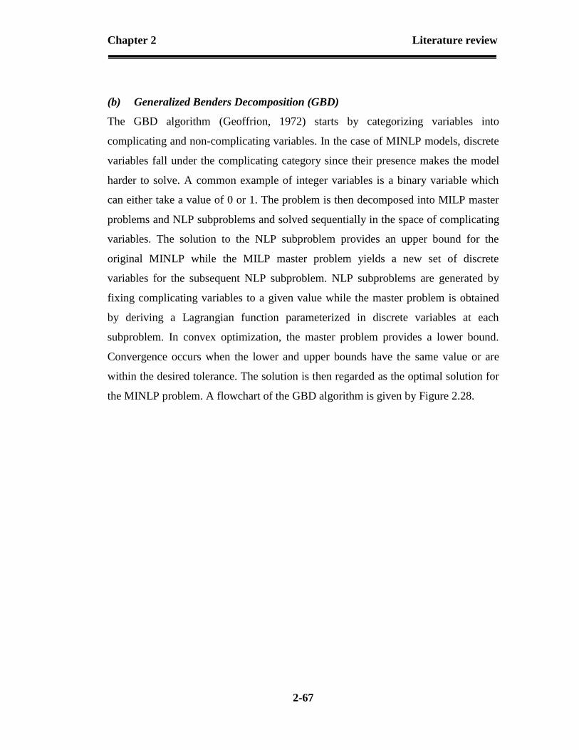
Chapter 2 Literature review
2-67
(b) Generalized Benders Decomposition (GBD)
The GBD algorithm (Geoffrion, 1972) starts by categorizing variables into
complicating and non-complicating variables. In the case of MINLP models, discrete
variables fall under the complicating category since their presence makes the model
harder to solve. A common example of integer variables is a binary variable which
can either take a value of 0 or 1. The problem is then decomposed into MILP master
problems and NLP subproblems and solved sequentially in the space of complicating
variables. The solution to the NLP subproblem provides an upper bound for the
original MINLP while the MILP master problem yields a new set of discrete
variables for the subsequent NLP subproblem. NLP subproblems are generated by
fixing complicating variables to a given value while the master problem is obtained
by deriving a Lagrangian function parameterized in discrete variables at each
subproblem. In convex optimization, the master problem provides a lower bound.
Convergence occurs when the lower and upper bounds have the same value or are
within the desired tolerance. The solution is then regarded as the optimal solution for
the MINLP problem. A flowchart of the GBD algorithm is given by Figure 2.28.

Chapter 2 Literature review
2-68
Original MINLP
Problem
Guess initial
values of y
Solve NLP
subproblem with
fixed yk
Solve MILP
Master problem
Is zU-zL< ɛ ?
Search stopped.
Optimum solution
found
k=k+1
Add integer cut to
get new y
Optimal solution: zU (upper bound)
Yes
No
Optimal solution: ZL (lower bound)
Figure 2.28 GBD and OA solution procedure for MINLP models
(c) Outer Approximation (OA)
The OA algorithm, developed by Duran and Grossman (1986) is similar to the GBD
method hence follows the same flowchart depicted by Figure 2.28. The difference
resides in the definition of the MILP master problem. In this case, the master problem
is obtained by performing an outer approximation, i.e. linearization or Taylor series
expansions, of the nonlinear constraints at optimal points of NLP subproblems
(Kallrath, 2000). This is graphically illustrated in Figure 2.29. For this reason, the OA
algorithm provides tighter bounds and requires fewer iterations for the problem to
converge when compared to the GBD algorithm.
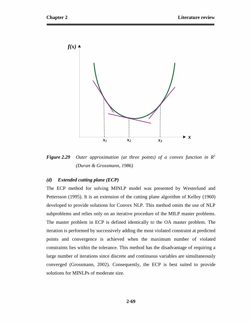
Chapter 2 Literature review
2-69
f(x)
xx1 x2 x3
Figure 2.29 Outer approximation (at three points) of a convex function in R1
(Duran & Grossmann, 1986)
(d) Extended cutting plane (ECP)
The ECP method for solving MINLP model was presented by Westerlund and
Pettersson (1995). It is an extension of the cutting plane algorithm of Kelley (1960)
developed to provide solutions for Convex NLP. This method omits the use of NLP
subproblems and relies only on an iterative procedure of the MILP master problems.
The master problem in ECP is defined identically to the OA master problem. The
iteration is performed by successively adding the most violated constraint at predicted
points and convergence is achieved when the maximum number of violated
constraints lies within the tolerance. This method has the disadvantage of requiring a
large number of iterations since discrete and continuous variables are simultaneously
converged (Grossmann, 2002). Consequently, the ECP is best suited to provide
solutions for MINLPs of moderate size.

Chapter 2 Literature review
2-70
2.6.4 Available optimization solvers for MINLP models
Various commercialized and open source solvers which can readily handle MINLP
problems are available to end-users and programmers. These algorithms differ from
each other by their built-in features to solve specific types of MINLP models to either
local or global optimality. MINLP algorithms often need to be customized for
specific MINLP problems amongst their wide range of applications. Moreover,
certain solvers for MINLP result from a combination of MIP, LP and NLP solvers.
The two aforementioned reasons explain why many commercial and free MINLP
solvers are embedded into modelling systems such as GAMS, AMPL, AIMMS, etc.
Nevertheless, there also exist many other solvers which can be readily used
independently of modelling languages (Bussieck & Vigerske, 2014).
The General Algebraic Modelling System (GAMS) is a well-established and user-
friendly modelling language which was introduced in 1970 and has been developed
and improved throughout the years. GAMS is designed to model and to solve linear,
nonlinear and mixed integer programming problems for complex and large scale
optimization problems. It contains both commercial and free solvers for MINLP
problems which include BARON, DICOPT, SCIP, LINDO, etc. A Mathematical
Programming Language (AMPL) and the Advance Interactive Mulltidimensional
Modelling System (AIMMS) are other widely used algebraic languages which both
appeared in the late 19’s (Fourer, et al., 1993; Bisschop & Roelofs, 1999). The NEOS
server is another robust server which gives access to more than fifty academic and
commercial optimization packages through internet interfaces. It was first announced
in 1995 and resulted from a collaborative and multi-institutional effort to develop
computational servers and cooperative technologies. It allows users to send tedious
and computational intensive optimization problems generated in either GAMS or
AMPL modelling systems and select the desirable solver among the available solvers
depending on the nature of the model (Dolan, et al., 2002).

Chapter 2 Literature review
2-71
The DICOPT (DIscrete and Continuous OPTimizer) algorithm is amongst the earliest
solvers capable of solving MINLP problems. It was developed by the research group
of I. E. Grossmann at the Engineering Design Center of Carnegie Mellon University
and is a commercial solver available within GAMS. The solution algorithm is based
on the OA algorithm of Duran and Grossmann (1986) and the Equality-Relaxation
(OA/ER) which is an extension of the OA performed by Kocis and Grossmann
(1987a) in conjunction with NLP advanced solvers such as MINOS. DICOPT can
guarantee global optimal solutions for convex MINLPs by using the OA algorithm
whereas, for nonconvex MINLPs, Equality Relaxation (ER) is introduced. It consists
of replacing nonlinear equality constraints with sets of inequalities constraints where
nonlinear functions are linearized. However, global optimum solutions are not
guaranteed for nonconvex MINLPs. The AOA (AIMMS Outer Approximation) can
also be named amongst OA based solvers. It is an open source solver integrated into
the AIMMS system.
There also exist Branch and Bound based MINLP solvers which use NLP relaxations.
Among them include the αBB (α-Branch-and-Bound) which was developed by the
research group of C. Floudas at the Computer-Aided Systems Laboratory of
Princeton University (Androulakis, et al., 1995). It is a global optimization solver for
nonconvex problems which is only made available to their research collaborators
(Bussieck & Vigerske, 2014). The SBB (Simple Branch-and-Bound) is another
branch and bound based commercial solver available within GAMS (GAMS
Development Corp., 2014).
Other types of solvers make use of convexification techniques in a branch and cut
algorithm to solve both convex and nonconvex models to global optimality. BARON
(Branch- And-Reduce-Optimization Navigator) is one of such algorithms. It is a
commercial solver that can be accessed within both AIMMS and GAMS. The Solver
implements a branch and bound procedure that use LPs for bounding and not NLPs as
used in conventional branch and bound technique for MINLP models. The Linear

Chapter 2 Literature review
2-72
relaxation of MINLP is obtained through linear outer approximation which entails
reformulating the problem by adding auxiliary variables such that it only contains
nonconvex terms for which convex underestimators or concave overestimators are
known. The branch and bound algorithm is enhanced by using duality techniques to
reduce the number of variables during the solution procedure (GAMS Development
Corp., 2014). ANTIGONE is another solver of that kind available within GAMS as a
commercial solver. Unlike BARON, ANTIGONE uses MIPs for bounding in the
branch and bound algorithm (Misener & Floudas, 2014)
2.7 Summary
This chapter gave detailed explanations of the various elements considered in the
design and optimization of a batch process. A literature review of the existing
techniques developed for the short-term scheduling of batch processes and the
minimization of wastewater generated by a batch water network was also performed.
It was observed that regeneration reuse, a technique used to minimize the
consumption of freshwater in batch processes, had not been thoroughly explored.
Moreover, no work that includes a detailed design model of a regeneration unit while
simultaneously optimizing batch schedule and water network had yet been performed.
This implies that the minimization of the amount of energy consumed by regeneration
units while optimizing the freshwater consumption of batch processes has been
overlooked. Therefore, the focus of this research study on developing a mathematical
formulation aiming to simultaneously minimize the freshwater use and regeneration
energy use of multipurpose batch processes while optimizing their production
schedule is justified. The next chapter will present and explain the novel
mathematical technique proposed for the optimization of multipurpose batch plants.

Chapter 2 Literature review
2-73
References
Adekola, O. & Majozi, T., 2011. Wastewater minimization in multipurpose batch
plants with a regeneration unit: Multiple contaminants. Computers and Chemical
Engineering, Volume 35, pp. 2824-2836.
Adekola, O. & Majozi, T., 2017. Wastewater minimization in batch plants with
sequence dependent changeover. Computers and Chemical Engineering, Volume
97, pp. 85-103.
Adjiman, C. S., Androulakis, I. P. & Floudas, C. A., 1997. Global optimization of
MINLP problems in process synthesis and design. Computers and Chemical
Engineering, Volume 21, pp. 445-450.
Almato, M., Espuna, A. & Puigjaner, L., 1999. Optimization of water use in batch
process industries. Computers and Chemical Engineering, Issue 23, pp. 1427-
1437.
Androulakis, I. P., Maranas, C. D. & Floudas, C. A., 1995. aBB: A global
optimization method for general constrained nonconvex problems. Journal of
Global Optimization, Volume 7(4), pp. 337-363.
Atasi, K. Z., 2015. Membrane technology advances wastewater treatment and water
reuse, s.l.: CDM Smith Inc.
Bisschop, J. J. & Roelofs, M., 1999. AIMMS. The user's guide, Haarlem: Paragon
Decision Technology B. V.
Bonvin, D., Srinivasan, B. & Hunkeler, D., 2006. Control and optimization of batch
processes: Improvement of process operation in the production of specialty
chemicals. IEEE Control Systems Magazine, pp. 34-45.
Borchers, B., 1992. Improved branch and bound algorithms for integer programming
, New York: Rensselaer Polytechnic Institute.
Bussieck, M. R. & Pruessner, A., 2003. Mixed Integer Nonlinear Programming,
Washington, DC: GAMS Development Corporation.
Bussieck, M. R. & Vigerske, S., 2014. MINLP solver software, Washington, DC:
GAMS Development Corporation.
Cerda, J., Henning, G. P. & Grossmann, I. E., 1997. A mixed-integer linear
programming model for short-term scheduling of single-stage multiproduct batch

Chapter 2 Literature review
2-74
plants with parallel lines. Industrial and Engineering Chemistry Research,
Volume 36, pp. 1695-1707.
Chang, C. T. & Li, B. H., 2006. Optimal design of wastewater equalization systems
in batch processes. Computers and Chemical Engineering, Volume 30, pp. 797-
806.
Chaturvedi, N. D. & Bandyopadhyay, S., 2012. A rigorous targeting to minimize
resource requirement in batch processes. Industrial and Engineering Chemistry
Research, Issue 51, pp. 8015-8024.
Chaturvedi, N. D. & Bandyopadhyay, S., 2013. Targeting for multiple resources in
batch processes. Chemical Engineering Science, Issue 104, pp. 1081-1089.
Chaturvedi, N. D. & Bandyopadhyay, S., 2014b. Simultaneously targeting for the
minimum water requirement and the maximum production in a batch process.
Journal of Cleaner Production, Volume 77, pp. 105-115.
Chaturvedi, N. D., Manan, Z. A., Alwi, S. R. W. & Bandyopadhyay, S., 2016. Effect
of multiple water resources in a flexible-schedule batch water network. Journal
of Cleaner Production, pp. 1-8.
Chaturvedi, N. D. & Bandyopadhyay, S., 2014a. Simultaneous targeting for the
minimum water requirement and the maximum production in a batch process.
Journal of Cleaner Production, Issue 77, pp. 105-115.
Chen, C.-L., Chang, C.-Y. & Lee, J.-Y., 2011. Resource-Task Network approach to
simultaneous scheduling and water minimization of batch plants. Industrial and
Engineering Chemistry Research, Volume 50, pp. 3660-3674.
Chen, C.-L. & Lee, J.-Y., 2008. A graphical technique for the design of water-using
networks in batch processes. Chemical Engineering Science, Issue 63, pp. 3740-
3754.
Cheng, K. F. & Chang, C. T., 2007. Integrated water network design for batch
processes. Industrial and Engineering Chemistry Research, Volume 46, pp.
1241-1253.
Dakin, R. J., 1965. A tree search algorithm for mixed-integer programming problems.
Computer Journal, Volume 8, pp. 250-255.
Dhamdhere, D. H., 2006. Operating systems: A concept-based Approach. 2nd ed.
New Delhi: Tata McGraw-Hill.
Dhole, V. R., Ramchandi, N., Tainsh, R. A. & Wasilewski, M., 1996. Make your
process water pay itself.. Chemical Engineering, Issue 103(1), pp. 100-103.

Chapter 2 Literature review
2-75
Dolan, E. D., Fourer, R., More, J. J. & Munson, T. S., 2002. Optimization on the
NEOS server. SIAM News, Volume 35, pp. 1-5.
Duran, M. A. & Grossmann, I. E., 1986. An outer-approximation algorithm for a
class of mixed-integer nonlinear programs. Mathematical Programming ,
Volume 36, pp. 307-339.
Edgar, T. F. & Himmelblau, D. M., 1988. Optimization of chemical processes. s.l.:
McGraw-Hill.
El-Halwagi, M. M., 1998. Pollution prevention through process integration. Clean
Products and Processes, Volume 1, pp. 5-19.
Ferrer-Nadal, S., Capon-Garcia, E., Mendez, C. A. & Puigjaner, L., 2008. Material
transfer operations in batch scheduling. A critical modelling issue. Industrial and
Engineering Chemistry Research, Volume 47, pp. 7721-7732.
Floudas, C. A. & Lin, X., 2004. Continuous-time versus discrete-time approaches for
scheduling of chemical processes: a review. Computers and Chemical
Engineering, Volume 28, pp. 2109-2129.
Foo, C., Manan, Z., Yunus, R. & Aziz, R., 2004. Synthesis of mass exchange network
for batch processes-Part I: Utility targeting. Chemical Engineering Science,
Volume 59, pp. 1009-1026.
Foo, C., Manan, Z., Yunus, R. & Aziz, R., 2005a. Synthesis of mass exchange
network for batch processes-Part II: minimum units target and batch network
design. Chemical Engineering Science, Volume 60, pp. 1349-1362.
Foo, C. Y., Manan, Z. A. & Tan, Y. L., 2005. synthesis of maximum water recovery
network for batch process systems. Journal of Cleaner Production, Volume 13,
pp. 1381-1394.
Foo, D. C. Y., 2010. Automated targeting for batch process integration. Industrial
and Engineering Chemistry Research, Issue 49, pp. 9899-9916.
Fourer, R., Gay, M. G. & Kernighan, B. W., 1993. A modelling language for
mathematical programming. San Fransisco: The Scientific Press.
GAMS Development Corp., 2014. GAMS - The Solver Manuals, Washington DC:
s.n.
Geoffrion, A. M., 1972. Generalized benders decomposition. Journal of Optimization
Theory and Applications, Volume 10(4), pp. 237-260.

Chapter 2 Literature review
2-76
Glover, F., 1975. Improved linear integer programming formulations of nonlinear
integer problems. Management Science, Volume 22, pp. 455-460.
Grossmann, I. E., 2002. Review of Nonlinear Mixed-Integer and Disjunctive
Programming Techniques. Optimization and Engineering, Volume 3, pp. 227-
252.
Gupta, O. K. & Ravindran, V., 1985. Branch and bound experiments in convex
nonlinear programming. Management Science, Volume 31 (12), pp. 1533-1546.
Harjunkoski, I. et al., 2014. Scope for industrial applications of production scheduling
models and solution methods. Computers and Chemical Engineering, Volume
62, pp. 191-193.
Ierapetritou, M. G. & Floudas, C. A., 1998. Effective continuous-time formulation for
short-term scheduling: 1. Multipurpose batch plants. Industrial and Engineering
Chemistry Research, Volume 37, pp. 4341-4359.
Judd, S. & Jefferson, B., 2003. Membranes for industrial wastewater recovery and
re-use. Oxford: Elsevier Ltd.
Kallrath, J., 2000. Mixed integer optimization in the chemical process industry.
Experience, potential and future perspectives. Trans IChemE, Volume 78, pp.
809-822.
Kelley, J. E., 1960. The cutting-plane method for solving convex programs. Journal
of SIAM, Volume 8, pp. 703-712.
Kim, J.-K. & Smith, R., 2004. Automated design of discontinuous water systems.
Trans IChemE, Part B, Process Safety and Environmental Protection, Issue
82(B3), pp. 238-248.
Kocis, G. R. & Grossmann, I. E., 1987a. Relaxation strategy for the structural
optimization of process flowsheets. Ind. Eng. Chem. Res., Volume 16(9), pp.
1869-1880.
Kondili, E., Pantelides, C. C. & Sargent, R. W. H., 1993. A general algorithm for
short term scheduling of batch operations-I. MILP formulation. Computers and
Chemical Engineering, Volume 17, pp. 211-227.
Korngold, E., 1982. Electrodialysis unit: Optimization and calculation of energy
requirement. Desalination, Volume 40, pp. 171-179.
Lee, H.-J., Sarfert, F., Strathmann, H. & Moon, S.-H., 2002. Designing of an
electrodialysis desalination plant. Desalination, Volume 142, pp. 267-286.

Chapter 2 Literature review
2-77
Lee, J.-Y., Chen, C.-L. & Lin, C.-Y., 2013. A mathematical model for water network
synthesis involving mixed batch and continuous units. Industrial & Engineering
Chemistry Research, Issue 52, pp. 7047-7055.
Lee, S. J., Alwi, S. R. W., Lim, S. L. & Manan, Z. A., 2014. Minimum water network
design for fixed schedule and cyclic operation batch processes with minimum
storage capacity and inter-connections. Journal of Cleaner Production, Volume
77, pp. 65-78.
Li, B. H. & Chang, C. T., 2006. A mathematical programming model for
discontinuous water-reuse system design. Industrial and Engineering Chemistry
Research, Volume 45, pp. 5027-5036.
Li, J. & Floudas, C. A., 2010. Optimal event point determination for short-term
scheduling of multipurpose batch plants via unit-specific event-based
continuous-time approaches. Industrial and Engineering Chemistry Research,
Volume 49, pp. 7446-7469.
Li, L.-J., Zhou, R.-J. & Dong, H.-G., 2010. Time-space superstructure-based MINLP
formulation for batch allocation network design. Industrial and Engineering
Chemistry Research, Volume 49, pp. 236-251.
Liu, W. B. & Floudas, C. A., 1993. A remark on the GOP algorithm for global
optimization. Journal of Global Optimization, Volume 3, pp. 519-521.
Liu, Y. et al., 2009. Optimal design of an integrated discontinuous water-using
network coordinating with a central regeneration unit. Industrial and
Engineering Chemistry Research, Volume 48, pp. 10924-10940.
Liu, Y., Yuan, X. & Luo, Y., 2007. Synthesis of water utilization system using
concentration interval analysis method (II) discontinuous process. Chin. J. Chem.
Eng., Issue 15(3), pp. 369-375.
Lundell, A., Skjal, A. & Westerlund, T., 2013. A reformulation framework for global
optimization. Journal of Global Optimisation, Volume 57, pp. 115-141.
Lundell, A. & Westerlund, T., 2012. Global optimization of mixed-integer signomial
programming problems. In: Lee J., Leyffer S. (eds) Mixed Integer Nonlinear
Programming.. The IMA volumes in mathematics and its applications, Volume
154. Springer, New York, NY, pp. 349-369.
Majozi, T., 2005a. An effective technique for wastewater minimization in batch
processes. Journal of Cleaner Production, Volume 13, pp. 1374-1380.

Chapter 2 Literature review
2-78
Majozi, T., 2005b. Wastewater minimization using central reusable water storage in
batch plants. Computers and Chemical Engineering, Volume 29, pp. 1631-1646.
Majozi, T., 2010. Batch Chemical Process Integration: Analysis, Synthesis and
Optimisation. London: Springer.
Majozi, T., Brouckaert, C. J. B. & Buckley, C. A. B., 2006. A graphical technique for
wastewater minimization in batch processes. Journal Environmental
Management, Volume 78, pp. 317-329.
Majozi, T. & Gouws, J. F., 2009. A mathematical optimisation approach for
wastewater minimisation in multipurpose batch plants: Multiple contaminants.
Computers and Chemical Engineering, Volume 33, pp. 1826-1840.
Majozi, T. & Gowns, J. F., 2009. A mathematical optimisation approach for
wastewater minimisation in multipurpose batch plants: Multiple contaminants.
Computers and Chemical Engineering, Volume 33, pp. 1826-1840.
Majozi, T. & Zhu, X. X., 2001. A novel continuous time MILP formulation for
multipurpose batch plants. 1. Short-term scheduling. Computer Aided Chemical
Engineering, Volume 9, pp. 937-942.
Mallevialle, J., Odendaal, P. E. & Wiesher, M. R., 1996. Water treatment: Membrane
processes. s.l.: McGraw-Hill.
Manan, Z. A., Tan, Y. L. & Foo, D. C. Y., 2004. targeting the minimum water
flowrate using water cascade analysis technique. AIChE, Volume 50, pp. 3169-
3183.
Maranas, C. D. & Floudas, C. A., 1995. Finding all solutions of nonlinearity
constrained systems of equations. Journal of Global Optimisation, Volume 7, pp.
143-182.
Maravelias, C. T. & Grossmann, I. E., 2003. New general continuous-time state-task
network formulation for short-term scheduling of multipurpose batch plants.
Industrial and Engineering Chemistry Research, Volume 42, pp. 3045-3074.
McCormick, G. P., 1976. Computability of global solutions to factorable nonconvex
programs: Part I - Convex underestimating problems. Mathematical
Programming, Volume 10, pp. 147-175.
Mendez, C. A. et al., 2006. State-of-the-art review of optimization methods for short-
term scheduling of batch processes. Computers and Chemical Engineering,
Volume 30, pp. 913-946.

Chapter 2 Literature review
2-79
Mintz, M. S. & Shaffer, L. H., 1980. Principles of desalination. New York:
Academic Press.
Misener, R. & Floudas, C. A., 2014. ANTIGONE: Algorithms for coNTinous /
Integer Global Optimization of Nonlinear Equations. Journal of Global
Optimization, 59(2-3), pp. 503-526.
Nie, Y., Biegler, L. T. & Wassick, J. M., 2012. Integrated scheduling and dynamic
optimization of batch processes using state equipment networks. AIChE Journal,
58(11), pp. 3416-3432.
Oliver, P., Rodriguez, R. & Udaquiola, S., 2008. Water use optimization in batch
process industries. Part 1: design of the water network. Journal of Cleaner
Production, Issue 16, pp. 1275-1286.
Ortiz, J. M. et al., 2005. Brackish water desalination by electrodialysis: Batch
recirculation operation modelling. J Membr Sci, Volume 525(1-2), pp. 65-75.
Pantelides, C. C., 1994. Unified frameworks for optimal process planning and
scheduling.. New York, Cache Publications.
Pinedo, M. & Chao, X., 1999. Operation scheduling with applications in
manufacturing and services, New York: McGraw-Hill.
Porn, R., Harjunkoski, I. & Westerlund, T., 1999. Convexification of different classes
of non-convex MINLP problems. Computers and Chemical Engineering,
Volume 23, pp. 439-448.
Quarteroni, A., 2009. Mathematical models in science and engineering, Milan: s.n.
Rohman, F. S. & Aziz, N., 2011. Optimization of batch electrodialysis for
hydrochloric acid recovery using orthogonal collocation method. Desalination,
Volume 275, pp. 37-49.
Sanmarti, E., Friedler, F. & Puigjaner, L., 1998. Combinatorial technique for short-
term scheduling of multipurpose batch plants based on schedule-graph
representation. Computers Chem. Engng, Volume 22, pp. S847-S850.
Schilling, E. & Pantelides, C. C., 1996. A simple continuous-time process scheduling
formulation and a novel solution algorithm. Computers and Chemical
Engineering, Volume 20, pp. 1221-1226.
Seid, E., 2013. On Synthesis, Design and Resource Optimization in Multipurpose
Batch Plants, Pretoria: University of Pretoria.

Chapter 2 Literature review
2-80
Seid, R. & Majozi, T., 2012a. A robust mathematical formulation for multipurpose
batch plants. Chemical Engineering Science, Volume 68, pp. 36-53.
Seid, R. & Majozi, T., 2012b. A novel technique for prediction of time points for
scheduling of multipurpose batch plants. Chemical Engineering Science, Volume
68, pp. 54-71.
Shaik, M. A. & Floudas, C. A., 2008. Unit-specific event-based continuous-time
approach for short-term scheduling of batch plants using RTN framework.
Computers and Chemical Engineering, Volume 32, pp. 260-274.
Shaik, M. A. & Floudas, C. A., 2009. Novel unified modeling approach for short-
term scheduling. Industrial and Engineering Chemistry Research, Volume 48,
pp. 2947-2964.
Shaik, M. A., Janak, S. L. & Floudas, C. A., 2006. Continuous-time models for short-
term scheduling of multipurpose batch plants: A comparative study. Industrial
and Engineering Chemistry Research, Volume 45, pp. 6190-6209.
Shaik, M. A. & Vooradi, R., 2013. Unification of STN and RTN based models for
short-term scheduling of batch plants with shared resources. Chemical
Engineering Science, Volume 98, pp. 104-124.
Silva, V., Poiesz, E. & van der Heijden, P., 2013. Industrial wastewater desalination
using electrodialysis: evaluation and plant design. J Appl Electrochem, Volume
43, pp. 1057-1067.
Strathmann, H., 2004. Assessment of electrodialysis for water desalination process
costs, Limassol: Institute of Chemical Engineering, University of Stuffgart,
Germany.
Sundaramoorthy, A. & Karimi, L. A., 2005. A simpler better slot-based continuous-
time formulation for short-term scheduling in multiproduct batch plants.
Chemical Engineering Science, Volume 60, pp. 2679-2702.
Susarla, N., Li, J. & Karimi, I. A., 2010. A novel approach to scheduling
multipurpose batch plants using unit slots. AIChE, Volume 56, pp. 1859-1879.
Tsiakis, P. & Papageorgiou, L. G., 2005. Optimal design of an electrodialysis
brackish water desalination plant. Desalination, Volume 173, pp. 173-186.
Wang, Y. P. & Smith, R., 1994. Wastewater minimisation. Chemical Engineering
Science, Volume 49, pp. 981-1006.
Wang, Y. P. & Smith, R., 1995. Time Pinch Analysis. Trans IChemE, Volume 73,
pp. 905-914.

Chapter 2 Literature review
2-81
Westerlund, T. & Pettersson, F., 1995. An extended cutting plane method for solving
convex MINLP problems. Computers Chem. Engng, Volume 19, pp. S131-S136.
Williams, H. P., 2013. Model building in mathematical programming. 5th ed.
Chichester: John Wiley & Sons Ltd.
Zhang, X. & Sargent, R. W. H., 1996. The optimal operation of mixed production
facilities-A general formulation and some approaches for the solution.
Computers and Chemical Engineering, Volume 20, pp. 897-904.
Zhang, Y. et al., 2012. RO concentrate minimization by electrodialysis: techno-
economic analysis and environmental concerns. J Environ manage, Volume
107C, pp. 28-36.
Zhou, R. J., Li, L. J., Xiao, W. & Dong, H. G., 2009. Simultaneous optimization of
batch process schedules and water allocation network. Computers and Chemical
Engineering, Volume 33, pp. 1153-1168.

3-1
MODEL DEVELOPMENT
3.1 Introduction
This chapter presents the mathematical model developed in this work to design and
synthesize a sustainable and cost-effective multipurpose batch plant. The MINLP
formulation is based on the superstructure depicted by Figure 3.1. It shows all
possible interconnections between batch processing units represented by j and j’, the
storage tanks and the regenerator. It is worth mentioning j and j’ can represent the
same units or different processing units that are directly integrated. Moreover, the
number of storage tanks as depicted by the superstructure is not subject to change.
This results from the fact that two storage tanks are required in order to connect batch
operations to the semi-continuous regeneration process. The proposed formulation is
divided into comprehensive sections depicting major components of the model
developed. This includes the scheduling model, the set of constraints for the water
balance around processing units and storage tanks, the set of constraints pertaining to
the design of the ED unit and finally constraints ensuring adequate sequencing of
tasks and events within the plant. Each aforementioned section is elaborated in this
chapter and the major assumptions made in the formulation are also stated.
3

Chapter 3 Model development
3-2
ED regenerator
jFreshwater
Direct reuse
from j’ to j
Direct reuse
from j to j’
Effluent
Wastewater
to storage
Diluate
Indirect reuse
/recycle
ED inlet stream
Reuse/ recycle
of diluate
Concentrate
Energy Consumption
j’
p,smw inj
e p,smw inj
f
p,k,sms effinj
out
p,smw inj
in p,smw inj
out
p,sms inj
in
in'js
in'j
injr p,s,smw
p,k,sms dilinj
out
in'js
inj
in'jr p,s,smw
fin Q,pmre
dil
out
Q
,pmre
conQ
Waste-
Water
Storage
Diluate
Storage
Figure 3.1 Water network superstructure for the proposed formulation
3.2 Scheduling model
The scheduling model ensures that the time dimension which is inherent in batch
processes is captured. It determines the time at which a specific task happens, the size
of the processed batch and the sequencing of tasks within a given time horizon. The
scheduling model adopted in this formulation was developed by Seid and Majozi
(2012). It is a unit specific slot-based formulation in which, for each unit, a
processing task and its subsequent washing operation are modelled to occur within
the same time slot p with unknown duration as illustrated in Figure 3.2. The model
has proven to be robust in terms of handling shared resources and requires fewer time
points compared to other formulations. The formulation includes allocation
constraints, material balance constraints, duration constraints, sequencing constraints,

Chapter 3 Model development
3-3
storage constraints for processing materials, tightening and time horizon constraints.
The details about the scheduling model are given in Appendix A
Units
Time
U1
p,sinj
Task
startsTask
ends
Washing
starts
Washing
ends
Task
starts
Task
ends
p,st inj
u p,st inj
p p,stw inj
u p,stw inj
p 1p,st inj
u 1p,st inj
p
p,sinj
w p,sinj
Figure 3.2 Scheduling model concept for batch processes
3.3 Material balance for the water network
3.3.1 Water balance constraints for washing operations
The material balance around each water-using operation is given by Constraints (3.1),
(3.2), and (3.3) following the superstructure depicted in Figure 3.1. Constraint (3.1)
states that the amount of water entering any processing unit at any time slot p is made
up of freshwater and/or the amount of water received from other units and storage
tanks. Constraint (3.2) states that the amount of water leaving a unit can be directly
reused to other processing units, sent to storage for later reuse and/or directly
disposed as an effluent. Constraint (3.3) ensures that the amount of water entering and
leaving an operation is conserved at any given slot p assuming no water loss in the
system.

Chapter 3 Model development
3-4
k
inj
out
s
inj
in'j
rinj
finj
in p,k,smsp,s,smwp,smwp,smwin'j
,
Kk,Ss,s,Pp inj
in'j
inj
(3.1)
p,smsp,s,smwp,smwp,smw inj
in
s
in'j
inj
rinj
einj
out
inj
,
inj
in'j
inj Ss,s,Pp
(3.2)
p,smwp,smw inj
outinj
in , inj
in'j
inj Ss,s,Pp (3.3)
Constraint (3.4) defines the amount of contaminant entering a unit at any given time
within slot p as the sum of the loads obtained from other processing units and from
storage tanks. Constraint (3.5) states that the amount of contaminant leaving a unit is
made up of the contaminant load to be removed after a task is processed in a unit and
the amount of contaminant in the inlet water stream. It is worth pointing out that the
contaminant load to be removed in each unit is modelled as a fraction of the size of
the batch that was processed in the unit prior to washing.
k
inj
outout
s
inj
in'j
rin'j
outinj
ininj
in
p,k,smsp,kcs
p,s,smwp,scp,smwp,scin'j
,
Kk,Ss,s,Pp inj
in'j
inj
(3.4)
p,smwp,scp,smusMp,smwp,sc inj
ininj
ininj
inj
inj
outinj
out ,
inj
in'j
inj Ss,s,Pp
(3.5)
Constraints (3.6) and (3.7) ensure that contaminant concentrations of water streams
entering and leaving processing units do not exceed their maximum allowable
concentrations. Alternatively, Constraint (3.7) can be modified by fixing the outlet
concentration of contaminants from each washing operation to its maximum

Chapter 3 Model development
3-5
allowable value. This is usually done in single contaminant problems to ensure that
the minimum possible amount of water is used in each operation.
p,sysCp,sc inj
inj
U,ininj
in , inj
inj Ss,Pp (3.6)
p,sysCp,sc inj
inj
U,outinj
out , inj
inj Ss,Pp (3.7)
Constraint (3.8) gives the limiting water requirement for each water operation. It is
the amount of water entering an operation at its maximum allowable inlet
concentration and exiting the operation at the maximum outlet concentration as
illustrated in Figure 3.3. As mentioned earlier, the contaminant load for each
operation is not fixed and depends on the batch size. Therefore, the maximum water
requirement is determined based on the assumption that the batch size of a specific
task occurring in a unit is equal to the capacity of the unit.
in
jU,inin
jU,out
inj
Ujin
jU
sCsC
sMVsW
,
inj
inj Ss (3.8)
Constraints (3.9), (3.10) and (3.11) ensure that the amount of water entering a unit at
any given slot p does not exceed the limiting water requirement.
p,sysWp,smw inj
inj
Uinj
in , inj
inj Ss,Pp (3.9)
p,s,sysWp,s,smw inj
in'j
rinj
Uinj
in'j
r , inj
in'j
inj Ss,s,Pp (3.10)
p,k,syssWp,k,sms inj
outinj
Uinj
out , Kk,Ss,Pp inj
inj (3.11)

Chapter 3 Model development
3-6
p,st inj
u p,st inj
p
inj
U,in sC
inj
U,out sC
inj
Uj sMV
Figure 3.3 Limiting water requirement for each washing operation (Majozi,
2005a)
3.3.2 Storage tanks modelling
The material balance around the storage tanks is given in Constraints (3.12) and
(3.13). Constraint (3.12) is the water balance around the wastewater storage tank. It
states that the amount of water stored at any given time slot p is the difference
between the amount stored and received from washing operations at the previous time
slot and the amount of water discharged to processing units and fed to the regenerator
at the current time point. Constraint (3.13) represents the water balance around the
diluate storage. It states that the amount of water stored at any given time slot p is the
amount previously stored and received from the regeneration process at the previous
time slot less the amount of water discharged to processing units at the current time
slot.
pmrepksms
psmspkqwpkqw
in
s
in
j
out
s
in
j
inss
inj
inj
,,
1,1,,
,(3.12)

Chapter 3 Model development
3-7
effinj
inj kk,Kk,Ss,pp,Pp 1
injs
inj
outoutss p,k,smspmrep,kqwp,kqw 11,
dilinj
inj kk,Kk,Ss,pp,Pp 1
(3.13)
Constraints (3.14) and (3.15) illustrate the water balance around storage tanks at the
first time slot. Constraints (3.14) states that the amount of water into the wastewater
storage at the first time slot is the difference between the amount of water that was
initially in storage and the amount of water discharged to processing units and fed
into the regenerator. Constraint (3.15) states that the amount of water stored in the
diluate storage tank within the first time slot is the amount of water initially stored in
the tank at the beginning of the time horizon less the amount of water transferred to
processing units for washing operations.
pmrep,k,smskQwp,kqw in
s
inj
outso
s
inj
,
effinj
inj kk,Kk,Ss,pp,Pp 1
(3.14)
injs
inj
outso
s p,k,smskQwp,kqw,
dilinj
inj kk,Kk,Ss,pp,Pp 1
(3.15)
Constraints (3.16), (3.17) and (3.18) ensure that both storage tanks are empty at the
end of the time horizon of interest. This implies that the amount of water stored and
partially purified at any given point in time is reused within the time horizon.

Chapter 3 Model development
3-8
0p,kqws, Kk,pp,Pp (3.16)
injs
inj
in p,sms 0,
inj
inj Ss,pp,Pp (3.17)
0pmreout, pp,Pp (3.18)
Constraint (3.19) is the contaminant balance around the wastewater storage tank. It
states that, at any point within slot p, the contaminant concentration of water
discharge by the tank is made up of the amount of contaminant remaining in storage
after discharging water at the previous slot and the amount received from other
processing units in the previous slot. Similarly, Constraint (3.20) stipulates the
contaminant balance around the diluate storage. It states that the amount of
contaminant into the outlet water stream from storage at any slot p is the sum of the
amount that remained in the amount received from the regenerator in the previous
slot. Constraint storage and the (3.21) states that, at the first time slot, the
contaminant concentration of the outlet water streams from storage tanks is equal to
the concentration of water that was initially found in the tanks at the beginning of the
time horizon.
pmrep,k,smsp,kqw
p,smsp,scp,kqwp,kcs
p,kcsin
s
inj
outs
s
inj
ininj
outsout
out
inj
inj
111
effinj
inj kk,Kk,Ss,Pp
(3.19)
injs
inj
outs
outoutsoutout
p,k,smsp,kqw
pmrepcrep,kqwp,kcsp,kcs
111
(3.20)

Chapter 3 Model development
3-9
dilinj
inj kk,Kk,Ss,Pp
kCsp,kcs outo
out , Kk,pp,Pp 1 (3.21)
Constraints (3.22), (3.23) and (3.24) ensure that the amount of water entering and
leaving storage tanks does not exceed the upper design bounds of storage tanks.
p,syskQsp,sms inj
inUinj
in , effin
jinj kk,Kk,Ss,Pp (3.22)
pykQspmre reUin , effkk,Kk,Pp (3.23)
pykQspmre reUout , dilkk,Kk,Pp (3.24)
It should be pointed out that the capacity of the storage tanks is not fixed beforehand.
Hence Constraints (3.25) - (3.29) ensure that optimum sizes of storage tanks are
obtained. Constraints (3.25) and (3.26) ensure that amount of water stored at any
point in time does not exceed the optimum tank size. Constraint (3.27) sets upper and
lower design bounds for storage capacity. Constraints (3.28) and (3.29) are associated
with the existence of storage tanks and ensure that storage exists prior to finding an
opportunity to transfer water to storage tanks.
injs
inj
inss p,smsp,kqwkv,
effinj
inj kk,Kk,Ss,Pp (3.25)
pmrep,kqwkv outss , dilkk,Kk,Pp (3.26)
kykQskvkykQs sUssL , Kk (3.27)
p,sysky inj
ins , effin
jinj kk,Kk,Ss,Pp (3.28)

Chapter 3 Model development
3-10
pyky res , dilkk,Kk,Pp (3.29)
3.4 ED design model
A detailed design of the electrodialysis regenerator is considered in this formulation.
The model was adapted from the work by Lee et al.(2002) and Tsiakis and
Papageorgiou (2005). In this formulation, the Electrodialysis membrane was designed
as a single stage process with feed-bleed adopted as the mode of operation as
illustrated in Figure 3.4. Constraints (3.30) – (3.50) represent the design equations
that characterize the electrodialysis membrane under the following assumptions.
(i) Cocurrent flow for stack operation as shown in Figure 3.4.
(ii) Membrane thickness is neglected.
(iii) The fluid is assumed to be Newtonian and flow to be laminar, incompressible
and fully developed.
(iv) Concentrate and diluate compartments have identical geometry for minimum
pressure difference, have equal flowrates and similar flow patterns.
(v) Water transport across membranes is negligible when compared to the
concentrate and diluate flowrates and concentrations.

Chapter 3 Model development
3-11
ff Q,C dildil Q,C
concon Q,C
df Q,C
mf Q,C
ddil Q,C
drdil Q,Ccc Q,C
cfc Q,C
crcon Q,C
Figure 3.4 Schematic representation of a single-stage electrodialysis
regeneration process
The material balance around the ED stack follows the schematic representation
illustrated in Figure 3.4. The mass balance equations are given by Constraints (3.30) -
(3.35). It is worth mentioning that Constraint (3.35) results from abovementioned
assumption of identical flowrates in diluate and concentrate compartments.
condilf QQQ (3.30)
mdf QQQ (3.31)
drdild QQQ (3.32)
crmc QQQ (3.33)
crdrccon QQQQ (3.34)
cd QQ (3.35)

Chapter 3 Model development
3-12
The corresponding contaminant balances are given in Constraints (3.36) - (3.39)
below.
concondildilff CQCQCQ (3.36)
conconconcrdildrcc CQCQCQCQ (3.37)
crcrfmfcc CQCQCQ (3.38)
ccdildfccfd CQCQCQCQ (3.39)
The feed split ratio m and the product recovery ratio r are given by Constraints (3.40)
and (3.41). The feed split ratio determines the ratio between the diluate flowrate and
the feed flowrate while the product recovery ratio determines the portion of the
diluate flowrate that is recovered as product of the electrodialysis process
f
d
Q
Qm
(3.40)
d
dil
Q
Qr
(3.41)
Constraint (3.42) is the design equation for the electric current consumed by the
electrodialysis stack. It is a function of the electrochemical valence z, the Faraday’s
constant F, the flowrate in the diluate compartmentdQ , the degree of desalination
C
, the current efficiency ɛ and the number of cell pairs N. The degree of desalination
defined by Constraint (3.43) is the portion of contaminant transferred from the diluate
to the concentrate compartment.

Chapter 3 Model development
3-13
N
CzFQI
del
(3.42)
fccondilf CCCCC (3.43)
The practical current density has been experimentally proven to be a function of the
linear velocity v (Lee, et al., 2013) as shown in Constraint (3.44). The constants aLCD
and bLCD in constraint (3.44) are determined experimentally by measuring the limiting
current density at various linear velocities (Lee, et al., 2002).
LCDbdilLCDprac vCai )( (3.44)
The flowrate in the diluate compartment is determined using the relationship
expressed by Constraint (3.45) below. It is a function of the cell thickness δ, the cell
width w and the spacer shadow factor α.
wvNQd (3.45)
In order to achieve a degree of cleanliness through electrodialysis, a total membrane
area is required as expressed by Constraint (3.46). The length of the ED stack is
defined as a function of the membrane area as shown in constraint (3.47).
praceq
c
dil
dildeq
fcdil
fc
iC
C
C
CzFQC
CC
CCln
A
1
(3.46)
wN
ALst
2 (3.47)

Chapter 3 Model development
3-14
The direct energy required for the regeneration process is given by Constraint (3.48).
It is dependent on the voltage applied to the stack and the current density. The applied
voltage is calculated using the relationship given in Constraint (3.49).
dil
elstdes
Q
IUE
(3.48)
C
cc
ccln
A
zFNCQU
eq
fcdilreg
freg
c
dst
(3.49)
Constraint (3.50) gives the mathematical expression for the energy required for
pumping the feed into the ED stack. It is a function of the pressure drop across the
stack and the pump efficiency. The pressure drop across the ED unit is expressed
using the relationship shown by Constraint (3.51) assuming a laminar flowrate.
p
trstpu kP
E
(3.50)
2
12
stst Lv
P (3.51)
The regenerator is modelled to operate semi-continuously at constant flowrate within
the time horizon. Constraints (3.52) and (3.53) link the amount of wastewater fed to
the regenerator to its actual feed flowrate. They ensure that the amount of water
transferred from storage to the regenerator at slot p is equal to the total quantity of
water fed into the ED for the duration regeneration process at time slot p. These
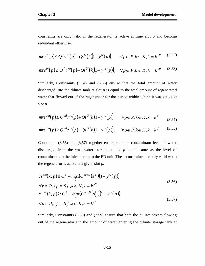
Chapter 3 Model development
3-15
constraints are only valid if the regenerator is active at time slot p and become
redundant otherwise.
pykQspQpmre reUrefin 1 , effkk,Kk,Pp
(3.52)
pykQspQpmre reUrefin 1 , effkk,Kk,Pp
(3.53)
Similarly, Constraints (3.54) and (3.55) ensure that the total amount of water
discharged into the diluate tank at slot p is equal to the total amount of regenerated
water that flowed out of the regenerator for the period within which it was active at
slot p.
pykQspQpmre reUredilout 1 , dilkk,Kk,Pp (3.54)
pykQspQpmre reUredilout 1 , dilkk,Kk,Pp
(3.55)
Constraints (3.56) and (3.57) together ensure that the contaminant level of water
discharged from the wastewater storage at slot p is the same as the level of
contaminants in the inlet stream to the ED unit. These constraints are only valid when
the regenerator is active at a given slot p.
pysCmaxCpkcs rein
j
Uout
s
fout
inj
1, ,,
effinj
inj kk,Kk,Ss,Pp
(3.56)
pysCmaxCpkcs rein
j
Uout
s
fout
inj
1),( ,,
effinj
inj kk,Kk,Ss,Pp
(3.57)
Similarly, Constraints (3.58) and (3.59) ensure that both the diluate stream flowing
out of the regenerator and the amount of water entering the diluate storage tank at

Chapter 3 Model development
3-16
time slot p have the same contaminant level. Again, the constraints hold only if the
regenerator is active at slot p, i.e. yre(p)=1.
pysCmaxCpcre reinj
U,out
s
dilout
inj
1 , inj
inj Ss,Pp (3.58)
pysCmaxCpcre reinj
U,out
s
dilout
inj
1 , inj
inj Ss,Pp (3.59)
3.5 Sequencing constraints for water network
This section consists of a set of constraints formulated to ensure that the discrete
nature of batch processes is captured, i.e. adequate sequencing of different events and
tasks within a given time horizon of interest.
In this formulation, water is used as a cleaning agent in washing operations which
occur after a task has been processed in a unit. Constraints (3.60) - (3.62) consist of
the sequencing constraints between batch tasks and washing operations. Constraint
(3.60) states that the duration of washing is the difference between the starting and
finishing time of a washing operation in a unit. Constraint (3.61) ensures that a
washing operation starts after the corresponding task is completed in a processing
unit. Constraint (3.62) states that a batch operation can start within slot p after the
completion of the washing operation at the previous time slot.
psyspstwpstw in
j
in
j
win
j
uin
j
p ,,, , inj
inj Ss,Pp (3.60)
p,stp,stw inj
pinj
u , inj
inj Ss,Pp (3.61)
1 p,stwp,st inj
pinj
u,
inj
inj Ss,pp,Pp 1 (3.62)
As mentioned earlier, this formulation explores both direct and indirect reuse
opportunities within a multipurpose batch plant. Constraints (3.63) – (3.65) describe

Chapter 3 Model development
3-17
the conditions to be fulfilled for direct reuse of water to occur between two
processing units. Constraint (3.63) states that for direct reuse to occur between two
washing operations, the operation receiving water must first take place, but the task
can still occur when no direct opportunities are found. Constraint (3.64) and (3.65)
together ensure that the finishing time of the task discharging water and the starting
time of the task receiving water coincide for direct reuse to occur.
p,syp,s,sy inj
inj
in'j
r , inj
in'j
inj Ss,s,Pp (3.63)
p,s,syHp,stwp,stw inj
in'j
rinj
uinj
p 1 ,inj
in'j
inj Ss,s,Pp (3.64)
p,s,syHp,stwp,stw inj
in'j
rinj
uinj
p 1 , inj
in'j
inj Ss,s,Pp (3.65)
Constraint (3.66) states that a washing operation must be scheduled to take place
prior to water being discharged from storage vessels to processing units. However,
the occurrence of a washing operation does not depend on whether an indirect reuse
opportunity is found at any given time slot p. Constraints (3.67) and (3.68) work
together to ensure that the time at which water is discharged from storage to a
processing unit coincides with the starting time of the washing operation in that unit.
p,syp,k,sys inj
inj
out , Kk,Ss,Pp inj
inj (3.66)
pksysHpstwpksts in
j
outin
j
uin
j
out ,,1,,, ,
Kk,Ss,Pp inj
inj
(3.67)
pksysHpstwpksts in
j
outin
j
uin
j
out ,,1,,, ,
Kk,Ss,Pp inj
inj
(3.68)
Constraint (3.69), similar to Constraint (3.66), states that the existence of an
opportunity to transfer water from washing operations to the wastewater tank depends

Chapter 3 Model development
3-18
on the occurrence of washing operations. Constraints (3.70) and (3.71) state that the
transfer time should be equal to the finishing time of the washing task for water to be
transferred from a processing unit to storage.
p,syp,sys inj
inj
in , inj
inj Ss,Pp (3.69)
p,sysHp,stwp,sts inj
ininj
pinj
in 1 , inj
inj Ss,Pp (3.70)
p,sysHp,stwp,sts inj
ininj
pinj
in 1 , inj
inj Ss,Pp (3.71)
Constraints (3.72) and (3.73) state that, if there are opportunities for water to be
discharged from storage to different processing units at the same time slot p, the
discharge time should be the same. These constraints ensure that all the streams
leaving storage have the same contaminant concentration at any given point within
time slot p. Constraint (3.74) ensures that the discharge time of water from storage to
processing units at earlier time slots is earlier than the discharge time at later time
slots.
p,k,sysp,k,sysH
p,k,stsp,k,sts
in'j
outinj
out
in'j
outinj
out
2 , Kk,Ss,s,Pp inj
in'j
inj (3.72)
p,k,sysp,k,sysH
p,k,stsp,k,sts
in'j
outinj
out
in'j
outinj
out
2 , Kk,Ss,s,Pp inj
in'j
inj (3.73)
'p,k,sysp,k,sysH'p,k,stsp,k,sts in
'joutin
jout
in'j
outinj
out 2
, Kk,Ss,s,p'p,P'p,p inj
in'j
inj
(3.74)

Chapter 3 Model development
3-19
Constraints (3.75), (3.76) and (3.77) are similar to constraints (3.72), (3.73) and
(3.74) respectively, but apply to opportunities where water is transferred from
processing units to storage.
p,sysp,sysHp,stsp,sts in'j
ininj
inin'j
ininj
in 2 ,
inj
in'j
inj Ss,s,Pp
(3.75)
p,sysp,sysHp,stsp,sts in'j
ininj
inin'j
ininj
in 2 ,
inj
in'j
inj Ss,s,Pp
(3.76)
'p,sysp,sysH'p,stsp,sts in'j
ininj
inin'j
ininj
in 2 ,
inj
in'j
inj Ss,s,p'p,P'p,p
(3.77)
Constraint (3.78) suppresses the opportunities for a storage tank to discharge and
receive water to and from different units at the same time slot. This is due to the fact
that the concentration of the outlet stream from storage at any given slot does not
cater for inlet streams within the slot. Constraint (3.79) states that opportunities to
transfer water from storage to processing units at earlier time slots p’ should occur
earlier than opportunities for the storage tank to receive water from processing units
at later time slots p. This constraint only holds when the described opportunities are
found during optimization, i.e. 1)( p,sys inj
in and 1)( 'p,k,sys in
'jout
.
1 p,k,sysp,sys in'j
outinj
in, Kk,Ss,s,Pp in
jin'j
inj (3.78)
'p,k,sysp,sysH'p,k,stsp,sts in'j
outinj
inin'j
outinj
in 2 ,
Kk,Ss,s,p'p,P'p,p inj
in'j
inj
(3.79)
The regenerator, which operates semi-continuously, receives and discharges water
from and to a storage tank. In order to know the time at which water starts being fed
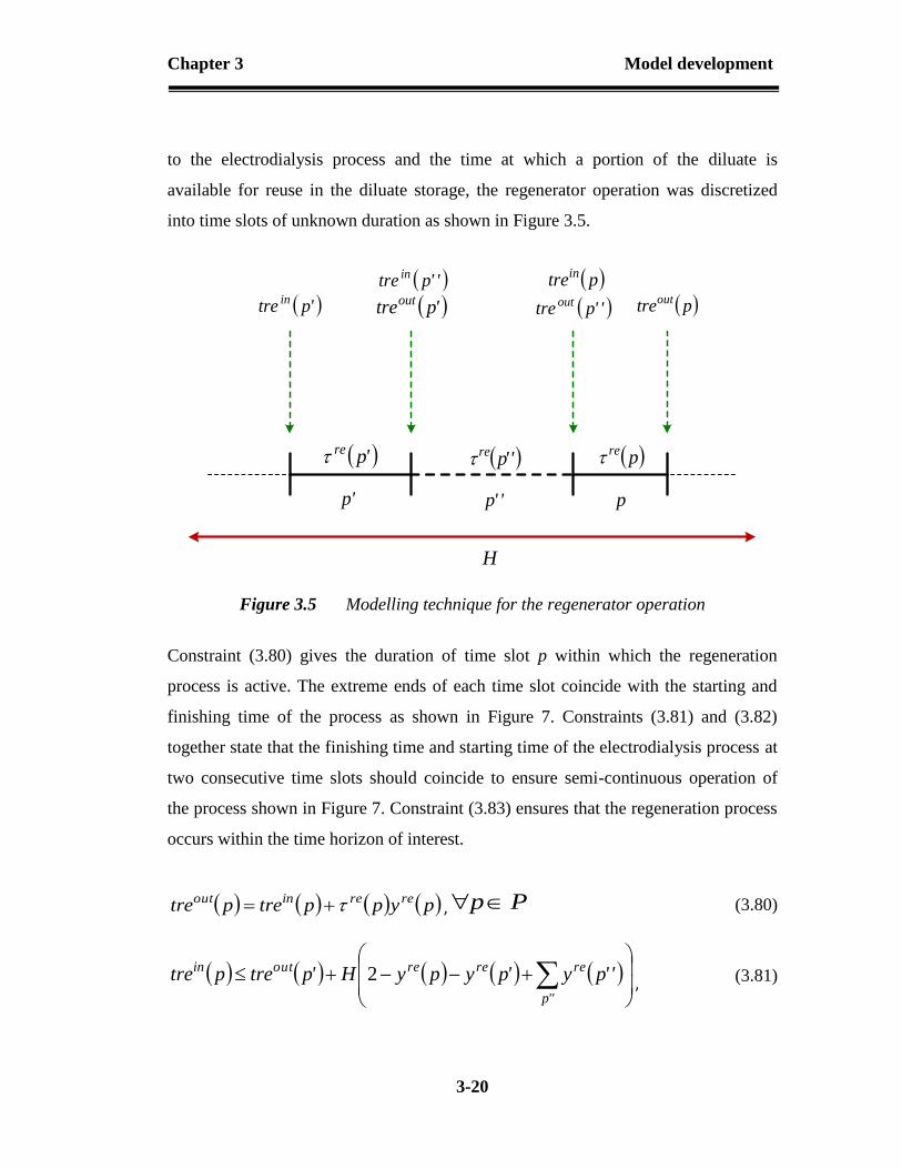
Chapter 3 Model development
3-20
to the electrodialysis process and the time at which a portion of the diluate is
available for reuse in the diluate storage, the regenerator operation was discretized
into time slots of unknown duration as shown in Figure 3.5.
p''p'p
H
'pre
'ptre in 'ptreout ''ptre out ptreout
''ptre in ptrein
''pre pre
Figure 3.5 Modelling technique for the regenerator operation
Constraint (3.80) gives the duration of time slot p within which the regeneration
process is active. The extreme ends of each time slot coincide with the starting and
finishing time of the process as shown in Figure 7. Constraints (3.81) and (3.82)
together state that the finishing time and starting time of the electrodialysis process at
two consecutive time slots should coincide to ensure semi-continuous operation of
the process shown in Figure 7. Constraint (3.83) ensures that the regeneration process
occurs within the time horizon of interest.
pypptreptre rereinout , Pp (3.80)
''p
rerereoutin ''py'pypyH'ptreptre 2, (3.81)

Chapter 3 Model development
3-21
'p''pp,P''p,'p,p
''p
rerereoutin ''py'pypyH'ptreptre 2,
'p''pp,P''p,'p,p
(3.82)
p
re Hp , Pp (3.83)
Constraint (3.84), similarly to constraint (3.78), ensures that the wastewater storage
does not receive water from processing unit and feed water to the ED unit within the
same time slot. Constraint (3.85) states that the time at which the regeneration
process starts within time slot p should be later than the time at which the wastewater
storage received water from processing units at previous time slots p’.
1 p,syspy inj
inre,
inj
inj Ss,Pp (3.84)
'p,syspyH'p,stsptre inj
inreinj
inin 2 ,
inj
inj Ss,p'p,P'p,p
(3.85)
Constraints (3.86) and (3.87) ensure that the wastewater storage tank discharges water
to processing units and feeds water to the regenerator at the same time if both events
occur within the same time slot p. Constraint (3.88) states that the discharge time of
water from storage to processing units at a previous time slot p’ should be earlier than
the time at which water is fed into the regenerator at a later time slot p.
p,k,syspyHp,k,stsptre inj
outreinj
outin 2 ,
effinj
inj kk,Kk,Ss,Pp
(3.86)

Chapter 3 Model development
3-22
p,k,syspyHp,k,stsptre inj
outreinj
outin 2 ,
effinj
inj kk,Kk,Ss,Pp
(3.87)
'p,k,syspyH'p,k,stsptre inj
outreinj
outin 2 ,
effinj
inj kk,Kk,Ss,p'p,P'p,p
(3.88)
Constraint (3.89) states that the diluate storage tank cannot discharge water to
washing operations and receive water from the regenerator within the same time slot
p. Constraint (3.90) ensures that the transfer of water from the regenerator to the
diluate tank at an earlier time slot p’ occur earlier than the discharge of water from
the tank to washing operations at a later slot p.
1 p,k,syspy inj
outre,
dilinj
inj kk,Kk,Ss,Pp (3.89)
p,k,sys'pyH'ptrep,k,sts inj
outreoutinj
out 2 ,
dilinj
inj kk,Kk,Ss,p'p,P'p,p
(3.90)
Constraints (3.91) – (3.98) ensure that every task, event and process integration
opportunity within the plant occur within the time horizon of interest.
Hp,st inj
u , inj
inj Ss,Pp (3.91)
Hp,st inj
p , inj
inj Ss,Pp (3.92)
Hp,stw inj
u , inj
inj Ss,Pp (3.93)
Hp,stw inj
p , inj
inj Ss,Pp (3.94)
Hp,sts inj
in , inj
inj Ss,Pp (3.95)

Chapter 3 Model development
3-23
Hp,k,sts inj
out , Kk,Ss,Pp inj
inj (3.96)
Hptrein , Pp (3.97)
Hptreout , Pp (3.98)
3.6 Objective function
The objective function of this formulation consists of maximizing the annualized
plant profit as illustrated by Constraint (3.99). It takes into account the production
revenue, the costs of freshwater and wastewater disposal, the capital and operating
costs of ED unit, as well as the installation and capital cost of storage tanks used.
nU,svsts
k
fst
max
pudesdileld
p
re
max
mb
d
p p s
reconinj
eew
s
inj
ffw
p
s
p
vCkyCt
EEH
QCt)p(A
t
C
H
t
pQp,smwCp,smwC
sqssSP
max
inj
inj
p
1
(3.99)
3.7 Nomenclature
The formulated mathematical model uses the following sets, parameters and
variables.
Sets
P { p|p represents a time point}

Chapter 3 Model development
3-24
J { j|j denotes a unit}
injS {
inj
inj s|s is an effective state representing a task performed in
unit j}
K { k|k is a storage tank}
pS { pp s|s is state representing a product}
Parameters
UjV capacity of unit j
H time horizon of interest
psSP selling price of product
injs duration of a processing task in unit j
inj
w s duration of washing in unit j
inj
U,out sC maximum allowable outlet concentration of water from unit j
inj
U,in sC maximum allowable concentration of water entering unit j
injsM mass load of contaminant to be removed in unit j
kQsU maximum amount of water that can be stored in storage tank k
kQs L minimum amount of water that can be stored in storage tank k
kQwso initial amount of water stored in storage tank k
kCsouto initial concentration of water stored in storage tank k
inj
U sW limiting water requirement in unit j
fwC freshwater cost in c.u/kg
ewC cost of wastewater treatment in c.u/kg
kCsouto initial concentration of water in storage k
LCDa constant for the limiting current density
LCDb constant for the limiting current density
F faraday constant
Chapter 3 Model development
3-25
elC electric power cost (c.u./kWh)
mbC membrane capital cost (c.u/m2) fstC installation cost of storage tanks (c.u)
vstC purchased cost of storage tanks (c.u/kg)
n cost coefficient of storage tanks
trk conversion factor
safety factor
maxt estimated maximum membrane equipment life
dt total operating time per year
w width of electrodialysis cell
z electrochemical valence
effective volume of cell factor (spacer)
effective area of cell factor (spacer shadow)
thickness of an electrodialysis cell
current utilization
p pump efficiency
viscosity of water
total resistance of anionic and cationic exchange membrane
eq equivalent conductance of water
rr removal ration of contaminant during regeneration process molM molecular mass of contaminant
Continuous Variables
p,smu inj amount of material processed by a task at time slot p
p,smw inj
in amount of water entering a unit at time slot p
p,smw inj
out amount of water entering a unit at time slot p
p,s,smw in'j
inj
r amount of water reused from unit j to j’ at time slot p
p,smw inj
e amount of water sent from unit j to effluent at time slot p
Chapter 3 Model development
3-26
p,smw inj
f amount of freshwater used in unit j at time slot p
p,sms inj
in amount of water transferred from unit j to storage at time slot p
p,k,sms inj
out amount of water transferred from storage k to unit j at time slot
p
pmrein amount of water transferred from storage to the regenerator at
time slot p
pmreout amount of water transferred from regenerator to storage at time
slot p
p,sqs p amount of product stored at time slot p
p,kqws amount of water stored in storage tank k at time slot p
p,sc inj
in concentration of water entering unit j at time slot p
p,sc inj
out concentration of water leaving unit j at time slot p
p,kcsout concentration of water leaving storage tank k at time slot p
pcreout concentration of water leaving the regenerator at time slot p
p,st inj
u starting time of a task at time slot p
p,st inj
p finishing time of a task at time slot p
p,stw inj
u starting time of washing task at time slot p
p,stw inj
p finishing time of washing task at time slot p
p,sts inj
in transfer time of from a unit to storage at time slot p
p,k,sts inj
out transfer time of water from storage tank k to unit j at time slot p
ptrein transfer time of water from storage to regenerator at time slot p
ptreout transfer time of water from the regenerator to storage tank at
time slot p
pre duration of regeneration process at time slot p

Chapter 3 Model development
3-27
kvs design capacity of storage tank k
A total membrane area required for desalination
fQ inlet feed flowrate to the regenerator
dilQ diluate product flowrate
conQ concentrate product flowrate
dQ diluate stream flowrate
cQ concentrate stream flowrate
mQ feed split flowrate
drQ diluate recycle stream flowrate
crQ concentrate recycle stream flowrate
fC concentration of inlet feed stream to the regenerator
dilC outlet concentration of diluate stream
conC outlet concentration of concentrate stream
fcC inlet concentration of concentrate stream
cC concentration of outlet concentrate compartment stream
crC concentration of concentrate recycle stream
desE specific desalination energy required by regenerator puE pumping energy required by regenerator elI electric current required by regenerator
praci practical limiting current density stL ED stack length
m ED feed split rate
r ED diluate product recovery rate
v linear ED flow velocity
stU voltage applied to the ED stack stP pressure drop across the ED stack

Chapter 3 Model development
3-28
Integer variables
N number of cell pairs required for desalination
Binary variables
p,sy inj binary variable associated with the assignment of a task at time
slot p
p,s,sy in'j
inj
r binary variable associated with the existence of a direct reuse
stream from j to j’ at time slot p
pyre binary variable associated with the existence of regeneration
process at time slot p
p,sys inj
in binary variable associated with the transfer of water from unit j
to storage time slot p
p,k,sys inj
out binary variable associated with the transfer of water from
storage to unit j
ky s binary variable associated with the existence of a storage tank k
References
Lee, H.-J., Sarfert, F., Strathmann, H. & Moon, S.-H., 2002. Designing of an
electrodialysis desalination plant. Desalination, Volume 142, pp. 267-286.
Lee, J.-Y., Chen, C.-L. & Lin, C.-Y., 2013. A mathematical model for water network
synthesis involving mixed batch and continuous units. Industrial & Engineering
Chemistry Research, Issue 52, pp. 7047-7055.
Majozi, T., 2005a. An effective technique for wastewater minimisation in batch
processes. Journal of Cleaner Production, Volume 13, pp. 1374-1380.
Seid, R. & Majozi, T., 2012. A robust mathematical formulation for multipurpose
batch plants. Chem. Eng. Sci., Volume 68, pp. 36-53.
Tsiakis, P. & Papageorgiou, L. G., 2005. Optimal design of an electrodialysis
brackish water desalination plant. Desalination, Volume 173, pp. 173-186.

4-1
ILLUSTRATIVE EXAMPLES
Introduction
The developed formulation was applied to two literature examples for verification
and practicability analysis. The resultant models for both examples were implemented
in GAMS 24.3.3 and solved using BARON. The computer used to solve the models
had the following specifications: Windows 7 Professional, Intel(R) Core ™ i7-4770
CPU @ 3.40GHz, 8.00 GB, and 64-bit Operating System.
Case study I
The first case study used for the verification of this formulation was adapted from
Halim and Srinivasan (2011). It is a simple batch plant that manufactures chemical D
using raw material A following the process illustrated in Figure 4.1. The production
line involves 3 tasks occurring in 5 units. Task 1 can be performed in units 1 and 2,
task 2 in unit 3 and task 3 in units 4 and 5. The operational philosophy of the plant
requires units 1, 2, 4 and 5 to be washed before the next batch is processed. Water is
used as a cleaning medium for the removal of residues remaining after processing a
task in a unit. Table 4.1 and Table 4.2 give a set of input parameters required for the
scheduling of the process. The information includes the available units and their
corresponding tasks, the processing time and washing time for each task, the amount
of raw material available in the plant, the storage capacity of raw materials,
4
Chapter 4 Illustrative Examples
4-2
intermediate materials and products, the selling price of products, as well as
freshwater cost and wastewater disposal costs. The duration of each task, i.e.,
processing time, is fixed and independent of the batch size as shown in Table 4.1.
Task 1
{Unit 1, Unit 2}
Task 2
{Unit 3}
Task 3
{Unit 4, Unit 5}A B C D
Washing Washing
Figure 4.1 State task network representation of the production recipe for case
study I
Table 4.3 gives a set of data pertaining to water integration for different tasks in their
respective units. This includes the maximum inlet and outlet contaminant water
concentrations as well as the contaminant mass load. The contaminant to be removed
in this case is sodium chloride (NaCl). It can be seen that task 2 occurring in unit 2
does not require washing; this explains why there is no data for maximum inlet and
outlet contaminant concentration for this task. Table 4.4 contains the parameters for
the design and costing of the ED unit and the storage tanks. The ED design and
costing input parameters were directly obtained from Tsiakis and Papageorgiou
(2005) while the costing parameters of a carbon steel storage tank were obtained from
Li and Chang (2006).The Chemical Engineering Plant Cost Index (CEPCI) was used
to account for the effect of years on the capital cost of storage tanks. The case study
focuses on a time horizon of 12h for short-term scheduling of the given plant.

Chapter 4 Illustrative Examples
4-3
Table 4.1 Production scheduling data for case study I
Units Suitability Maximum
batch size
(kg)
Processing time (h) Washing
time (h)
Unit 1 Task 1 100 1.25 0.25
Unit 2 Task 1 150 1.7 0.30
Unit 3 Task 2 200 1.5 0.00
Unit 4 Task 3 100 0.75 0.25
Unit 5 Task 3 150 1.2 0.30
Table 4.2 Additional scheduling data for case study I
Material state Initial inventory Max storage
(kg)
Revenue or cost (c.u/kg)
A 1000 1000 0
B 0 200 0
C 0 200 0
D 0 1000 5
Freshwater - 200 0.1
Wastewater - 150 0.05
Table 4.3 Process integration data for washing tasks in case study I
Units Suitability Max inlet
concentration
(ppm)
Max outlet
concentration
(ppm)
Contaminant
loading (g NaCl/kg
batch)
Unit 1 Task 1 500 1000 0.2
Unit 2 Task 1 50 100 0.2
Unit 3 Task 2 - - -
Unit 4 Task 3 150 300 0.2
Unit 5 Task 3 300 2000 0.2

Chapter 4 Illustrative Examples
4-4
Table 4.4 Additional parameters for the design and costing of the ED unit and
storage tanks for case study I and II
Parameters Symbols Value
Limiting current density constant LCDa 2500
Limiting current density constant LCDb 0.5
Faraday’s constant, A s/keq F 96,500,000
Conversion factor, kWh/J trk 27.2
Safety factor 0.7
Cell width, m w 0.42
Cell thickness, m 0.00065
Effective volume of cell factor (spacer) 0.8
Effective cell factor volume (spacer
shadow) 0.7
Current utilization 0.9
Pump efficiency p 0.7
Solution viscosity, kg/ m s 0.000984
Total resistance of membranes, Ω m2 0.0007
Equivalent conductance of solutions, s
m2/keq eq 10.5
Contaminant removal ratio rr 0.95
Membrane capital cost, c.u./m2 mbC 150
Electric power cost, c.u./kWh elC 0.12
Storage tank fixed cost , c.u. fstC 50,000
Storage tank purchased cost, c.u./kg vstC 280
Storage tank cost coefficient n 0.6
Estimated maximum equipment life, y maxt 5
Operating time per year, s dt 28,512,000

Chapter 4 Illustrative Examples
4-5
4.2.1 Computational results and discussion
The solution of the formulation yielded the plant schedule as shown in Figure 4.2.
Figure 4.2 shows the optimum sequence of batch processing tasks and their
subsequent washing operations from unit 1 to unit 5. It also shows the resultant water
network where different arrows illustrate different opportunities for water reuse as
well as freshwater streams. For example, the second washing operation in unit 2
received 190.8kg from the freshwater source and the same amount from the
wastewater storage tank. At the end of the operation, 204.2 kg of wastewater was then
sent to the wastewater storage tank for later reuse and the remaining amount, i.e.
177.4 kg, was discharged as effluent. The optimum feed, diluate and concentrate
flowrates around the ED regenerator were found to be 100.8 kg/h, 95.8 kg/h, and 5
kg/h respectively. The sizes of batch processing tasks in each unit are also displayed
in Figure 4.2. Illustratively, unit 1 processed 6 batches of 100 kg each, while unit 2
processed 4 batches of 104.6 kg, 95.4 kg, 100 kg and 100 kg respectively. The
wastewater reusable storage and the diluate storage were found to have optimum
sizes of 222.6 kg and 189.8 kg respectively.
From Table 4.3, it can be observed that washing operations in unit 2 have the lowest
inlet and outlet contaminant restrictions. As a result, effluents from unit 2 are easily
reused in all other units but effluents from the other 3 units are not directly or
indirectly reused to unit 2 without purification or dilution. Therefore, the regenerator
is operated continuously for 2h in order to partially purify a portion of wastewater
and facilitate reuse in unit 2. The model also found opportunities for wastewater from
the wastewater storage to be diluted with freshwater and reuse in unit 2 as a way of
minimizing freshwater use and the cost of wastewater regeneration.
Table 4.5 gives a comparative study between the results obtained from a base case
model with those obtained using the proposed formulation. The base case model
includes constraints pertaining to scheduling and water balance. It considers
freshwater as the only available water source to satisfy all water-using operations.

Chapter 4 Illustrative Examples
4-6
This implies that no reuse opportunity for water is explored among processing units.
It can be seen from Table 4.5 that the proposed formulation allowed the plant to save
37.4 % of the initial amount of freshwater used when no integration was employed.
However, the CPU time drastically increased from 0.2 to 28,782 seconds. This is
explained by the higher number of constraints, variables and nonlinear terms that the
resultant formulation entails as shown in Table 4.5.
Table 4.5 Comparative results for case study I
No integration Proposed formulation
Annual Profit (c.u×105) - 32.3
Freshwater (kg) 1,105 691.2
Revenue (c.u) for 12h
horizon
5,000 5,000
Percentage freshwater
saving
- 37.4
No. constraints 905 5,295
No. variables 555 1,486
No. discrete variables 75 348
No. binary variables 75 248
Non-linear terms 64 998
CPU time (s) 0.32 28,782
The complexity of the resulting model is explained by the fact that the model
attempts to synthesize a water network while designing the regeneration process and
optimizing the schedule of the plant. Hence the formulation is more suited for the
design phase of the batch plant. However, the operation phase will reduce the
problem to a synthesis problem and further simplification can occur for processes
where the schedule of the plant is not subject to change. Table 4.6 gives the design
parameters pertaining to the regenerator suitable for the process described in this case

Chapter 4 Illustrative Examples
4-7
study. It includes the total membrane area required for the resultant plant set up, the
number of cell pairs in the ED stack, the length of the stack, etc. The total pumping
and desalination energy required for the process are also given in Table 4.6.
Table 4.6 Design specifications of the ED regenerator for case study I
Design variables Optimum values
Membrane area(m2) 7.1
No. cell pairs 12
ED stack length(m) 0.7
Desalination energy (kWh/y) 3.632
Pumping energy (kWh/y) 0.078
Electric current (A) 0.651
Product recovery rate 0.95
Linear velocity(m/s) 0.011
The implication of implementing a detailed regeneration model as opposed to
adopting a black-box approach was investigated. Table 4.7 compares the results
obtained from the proposed mathematical formulation with an embedded ED model
to those obtained when the ED model is replaced with a black-box regenerator model.
The black-box model used the same removal ratio and liquid recovery as the ED
design model. The case where the objective function of the black-box formulation
does not include the regeneration cost was considered in the presented black-box
approach. It can be seen, from Table 4.7, that the black-box approach achieved 57.5
% reduction in freshwater consumption as opposed to the 37.4 % achieved by the
proposed formulation. However, the higher reduction in freshwater consumption
entailed an increase in the amount of water fed to the regenerator unit, in the duration
of the regenerator operation within the makespan, in the total amount of energy
consumption, and in the size of storage tanks. As a result, a 13.3 % reduction in the
total cost of the water network was observed when adopting the proposed formulation

Chapter 4 Illustrative Examples
4-8
as opposed to the black-box approach. The total cost of water network as given in
Table 4.7 accounted for the cost of freshwater, the cost of wastewater treatment and
disposal, the capital and operating cost of regeneration and the cost of storage. The
production revenue was not included in the cost analysis because it was kept at its
maximum value in both approaches.
The total energy consumed by the regenerator when adopting the black-box approach
was obtained by performing a two-step optimization. Firstly, the black-box model
was solved wherein the plant profit was maximized by considering the production
revenue, the freshwater and wastewater cost. The second step consisted of optimizing
the capital and operational cost of regeneration using the electrodialysis standalone
model. The flowrates and contaminant concentrations around the regenerator were
fixed to the value obtained in the first step. The total energy consumption of the
regenerator within the time horizon was then calculated. A comparison between the
results obtained from this technique and the proposed optimization approach shows
that a 31.6 % reduction in energy consumption was achieved when adopting the
proposed formulation instead of using the black-box modelling approach.
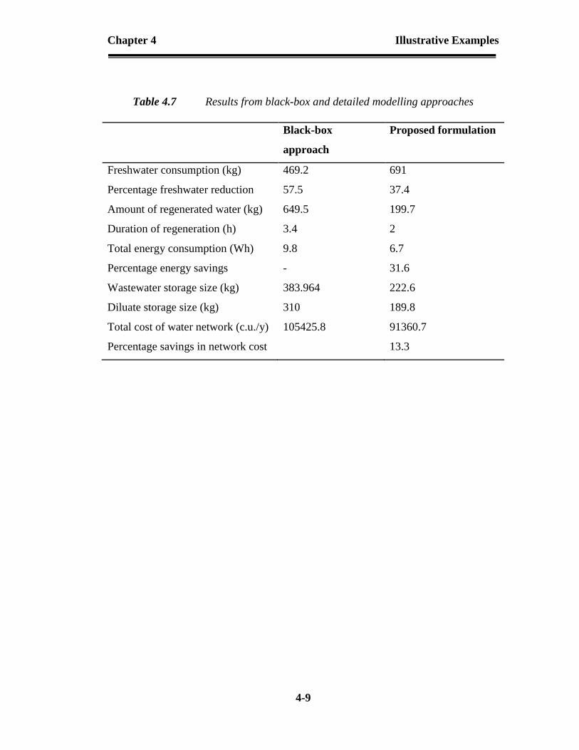
Chapter 4 Illustrative Examples
4-9
Table 4.7 Results from black-box and detailed modelling approaches
Black-box
approach
Proposed formulation
Freshwater consumption (kg) 469.2 691
Percentage freshwater reduction 57.5 37.4
Amount of regenerated water (kg) 649.5 199.7
Duration of regeneration (h) 3.4 2
Total energy consumption (Wh) 9.8 6.7
Percentage energy savings - 31.6
Wastewater storage size (kg) 383.964 222.6
Diluate storage size (kg) 310 189.8
Total cost of water network (c.u./y) 105425.8 91360.7
Percentage savings in network cost 13.3

4-10
104.6
86.5
10
95.4
200
150
100
100
113.5
150
100
100
200
100
150
100
200
100
150
100
200
100
0 1 2 3 4 5 6 7 8 9 10 11 12
Unit 1
Unit 2
Unit 3
Unit 4
Unit 5
Storage
Regenerator
100
63.5
100
26.5
222.6 189.8
20 20 2020
209.2
190.8
10.2 200
1.0
189.8
190.8
6.7
22.2 22.2
26.5 100 133.3
15.8
209.2 204.2 138 106.7
26.5 33.3
62
100
17.617.6 17.6
100.8 kg/h
95.8 kg/h
5.0 kg/h
Hours
20 20 22.2 20 22.2 20
177.4
1.0 17.6 17.6 17.6
15.8
44.4 100
49.1 115.7WW
FW
Freshwater streams
Inlet streams to tank 1
Outlet streams from tank 1
Outlet streams from tank 2
Direct reuse streams
ED inlet and outlet streams
Wastewater effluents
Figure 4.2 Gantt chart for case study I

Chapter 4 Illustrative Examples
4-11
Case study II
The second example is adapted from Kondili et al. (1993) who first presented the case
study for the validation of their scheduling model, and Halim and Srinivasan (2011)
who included additional data required for water integration. The case study consists
of a multipurpose batch plant which aims to manufacture two products using three
different raw materials. The production recipe involves a preheating process, three
reactions occurring in two reactors and a separation process. Figure 4.3 gives the STN
and SSN representation of the recipe to be followed for the manufacturing of products
1 and 2. It also shows, for each task, the percentage of feed required and percentage
of intermediate and final products to be produced. Table 4.8 and Table 4.9 contain
input parameters essential for the scheduling of the plant. It is worth mentioning that
this case study considers the processing time of a task to be dependent on its batch
size. Table 4.10 gives a set of parameters pertaining to washing operations for units
with cleaning requirements with magnesium chloride (MgCl2) being the contaminant
to be removed. From Table 4.10, it can be seen that washing operations are only
required for the two multipurpose reactors to avoid contamination between the three
different reactions occurring in these units.

Chapter 4 Illustrative Examples
4-12
Feed A
Feed B
Feed C
Hot A
Int BC
Int AB
Product 1
Impure E
Product 2
50%
50% 60%
40%40%
60%
20%
80%
90%
10%
Heating
Reaction 2Reaction 1
Reaction 3
Separation
s1 s5
s2
50%
50%
s6
40%
60%
s7
40%
s8
60%
80%
20%
s9
10%
s10
90%
(s1)
(s2)
(s3)
(s4)
(s5)
(s6)
(s7)
(s8) (s9)
(s10)
Feed A
Feed B
Feed C
(s3)
(s4)
Hot A
Int BC
Int BC
Product 1
Product 2
Impure E
(a) SSN representation
(b) STN representation
Figure 4.3 SSN and STN representation for production recipe of case study II

Chapter 4 Illustrative Examples
4-13
Table 4.8 Production scheduling data for case study II
Units Suitability Capacity Fixed
processing
time (h)
Variable
processing
time (h)
Washing
time (h)
Heater Heating 100 0.667 0.007 0.00
Reactor
1
Reaction 1 50 1.334 0.027 0.25
Reaction 2 50 1.334 0.027 0.25
Reaction 3 50 0.667 0.013 0.25
Reactor
2
Reaction 1 80 1.334 0.017 0.30
Reaction 2 80 1.334 0.017 0.30
Reaction 3 80 0.667 0.008 0.30
Still Separation 200 1.334 0.007 0.00
4.3.1 Results and discussions
Table 4.11 gives the computational results for case study II and compares them with
results obtained from the case where no process integration was employed. For this
case study, the proposed formulation was able to reduce freshwater intake by 41.1%
while maintaining the same production revenue. It is worth mentioning that the base
case, i.e. the formulation with no integration, does not cater for additional costs of the
water network such as regeneration and storage costs. Hence, no comparison was
performed between the two cases in terms of the annualized plant profit as shown in
Table 4.11. Table 4.11 also gives the model statistics for both cases and, similar to
the first case study, the proposed formulation yielded a higher CPU time.

Chapter 4 Illustrative Examples
4-14
Table 4.9 Additional scheduling data for case study II
Material state Initial inventory Max storage
(kg)
Revenue or cost (c.u/kg)
Feed A 1000 1000 10
Feed B 1000 1000 10
Feed C 1000 1000 10
Hot A 0 100 0
Int AB 0 200 0
Int BC 0 150 0
Impure E 0 200 0
Product 1 0 1000 20
Product 2 0 1000 20
Freshwater - - 0.1
Wastewater - - 0.05
Table 4.10 Process integration data for tasks requiring washing for case study II
Units Task Max inlet
concentra-
tion (ppm)
Max outlet
concentration
(ppm)
Contaminant
loading (g
MgCl2/kg batch)
Heater Heating - - -
Reactor 1 Reaction 1 500 1,000 0.2
Reaction 2 10 200 0.2
Reaction 3 150 300 0.2
Reactor 2 Reaction 1 50 100 0.2
Reaction 2 30 75 0.2
Reaction 3 300 2,000 0.2
Still Separation - - 0.2

Chapter 4 Illustrative Examples
4-15
The Gantt chart obtained as a result of the implementation of the proposed
formulation for this case study is shown in Figure 4.4 It gives the sequence of tasks
and network configuration the plant has to follow in order to achieve the optimum
plant profit given in Table 4.11. The model yielded a water network with
opportunities for freshwater use, indirect and regeneration reuse whilst no direct reuse
opportunities where found. The regenerator operated for 2.6h with the process
starting at time 5.9h within the time horizon. The delay in the starting time of the
regeneration process is explained by the fact that the wastewater storage tank needed
to have a considerable amount of water to allow the ED regenerator to operate
continuously. The short operation time of the regenerator is due to the fact that this
formulation forces both the diluate and wastewater storages to be empty at the end of
the time horizon of interest. In a cyclic scheduling problem, this constraint could be
relaxed to allow for reuse between different production cycles within the facility. The
design specifications of the ED regenerator required for this plant are given in Table
4.12. The regenerator is ED stack of 0.7 m length which contains 10 cell pairs and
requires a total membrane area of 5.9 m2. The energy requirements, flow velocity and
process efficiency of the electrodialysis regenerator are also included in Table 4.12.

Chapter 4 Illustrative Examples
4-16
Table 4.11 Detailed results for case study II
No integration Proposed formulation
Annual Profit (c.u×105) - 31
Freshwater (kg) 735.0 430.4
Revenue (c.u) for 12h
horizon
4665.3 4665.3
Percentage freshwater
saving
- 41.4
No. constraints 1,548 3,798
No. variables 794 1,420
No. discrete variables 104 325
No. binary variables 104 225
Non-linear terms 84 848
CPU time (s) 1.49 28,000
Table 4.12 Design specifications for the ED unit in case study II
Design variables Optimum values
Membrane area(m2) 5.9
No. cell pairs 10
ED stack length(m) 0.7
Desalination energy (kWh/y) 1.101
Pumping energy (kWh/y) 0.096
Electric current (A) 0.400
Product recovery rate 0.95
Linear velocity(m/s) 0.013
The advantages of adopting the proposed mathematical formulation over a black-box
approach are demonstrated in Table 4.13. It compares the water network

Chapter 4 Illustrative Examples
4-17
specifications obtained using the proposed formulation with those obtained using the
black-box approach described in Section 4.2.1. It can be seen that both approaches
gave the same freshwater consumption whilst an increase in the amount of
regenerated water was observed in the black-box approach. As a result, the size of
storage tanks and the amount of energy consumed increased, resulting in a higher cost
of the water network. The proposed formulation achieved the same water
consumption by favouring the exploration of direct and indirect reuse which came at
a lower cost compared to feeding the regenerator with more wastewater as suggested
by the black-box approach. Therefore, a 0.56 % and 9.87 % decrease in water
network cost and energy consumption respectively was achieved by the proposed
optimization approach. This demonstrates the importance of designing a regeneration
operation with enough details to enable the objective function of an optimization
problem to capture its accurate cost.
Table 4.13 Comparative results from black-box and detailed modelling
approaches
Blackbox approach Proposed formulation
Freshwater consumption (kg) 430.4 430.4
Amount of regenerated water (kg) 289 259.4
Duration of regeneration (h) 1.4 2.6
Total energy consumption (Wh) 3.5 3.1
Percentage energy savings - 9.87
Wastewater storage size (kg) 369.6 259.7
Diluate storage size (kg) 274.6 246
Total cost of water network (c.u./y) 66257 65884.3
Percentage savings in network cost - 0.56

4-18
R1(50)
R1(80)
R2(49.9)
R2(78.9)
R3(50)
R2(80)
R3(37.6)
R3(44)
R3(31.3) R2(7.8)
0 1 2 3 4 5 6 7 8 9 10 11 12
Heater
Reactor 1
Reactor 2
Still
Storage
Regenerator
50
86.7
112.9
259.7
246.2
160210.5
10 49.9 33.3
48.7
210.5
32.4
213.3
25 7.827.8
4.6
98.5 kg/h 5 kg/h
93.5 kg/h
111.3 180.9
4.6
10 49.9 33.3 25 27.8 7.8
FW
WW
Freshwater
Inlet streams to tank 1
Outlet streams from tank 1
Outlet streams from tank 2
ED inlet and outlet streams
Wastewater effluents
Figure 4.4 Gantt chart for case study II

Chapter 4 Illustrative Examples
4-19
References
Halim, I., & Srinivasan, R. (2011). Sequential methodology for integrated optimization of
energy and water use during batch process scheduling. Comput. Chem. Eng., 35, 1575-
1597.
Kondili, E., Pantelides, C. C., & Sargent, R. W. (1993). A general algorithm for short-term
scheduling of batch operations. I. MILP formulation. Computers and Chemical
Engineering(17), 211-227.
Li, B., & Chang, C. (2006). A mathematical programming model for discontinuous water-
reuse system design. Industrial and Engineering Chemistry Research, 45, 5027-5036.
Tsiakis, P., & Papageorgiou, L. G. (2005). Optimal design of an electrodialysis brackish
water desalination plant. Desalination, 173, 173-186.

5-1
INDUSTRIAL CASE STUDY
5.1 Introduction
Dairy processing plants require a considerable amount of water to maintain standard
levels of cleanliness and hygiene and avoid any growth of pathogenic
microorganisms which can cause serious health hazards. A case study on the
reduction of water consumption was undertaken at Amul processing plant, one of the
biggest producers of dairy products in both India and the world. Raw milk is
collected from approximately 700 thousand villagers and processes 1800 cubic meter
of milk per day while the daily water requirement is currently set at 1600 cubic
meters (Buabeng-Baidoo, et al., 2017). Their main products are milk, ghee, butter,
flavoured milk and milk powder. The plant is accordingly divided into the raw milk
receiving department (RMRD), powder, ghee, flavoured milk, skimmed milk powder
and milk packaging sections as shown in Figure 5.1. The total annual consumption of
water in this plant is currently at six millions of cubic meter per annum. 75% of the
total water consumed is used in cleaning in place (CIP) and floor cleaning processes
while the remaining 25% is directed to other operational duties as shown in Figure
5.2. These duties include the usage of water for cooling tower make up, boiler feed
make up, operational processes, railway tanker wash, and many other processes.
5

Chapter 5 Industrial Case Study
5-2
Raw milk receiving and
processing department
(RMRD)
Powder
PlantButter
Section
Ghee
Section
Flavoured
Milk
Skimmed
Milk Powder
Plant
Milk
Packaging
Figure 5.1 Amul dairy production plant scheme
Figure 5.2 Distribution of water consumption in Amul dairy plant
CIP is an automated cleaning procedure of various processing units, pipes, tanks and
other facilities to maintain the required hygiene standards. It involves the use of
75%
3%
2%2%
16%
2%
CIP and Floor cleaning
Operational processes
Railway tanker wash
Cooling tower makeup
Boiler feed makeup
other

Chapter 5 Industrial Case Study
5-3
controlled valves and pumps to achieve programmed water flow and circulation when
required. Traditional cleaning in the dairy industry was performed by plant operators
who used to disassemble the equipment to be cleaned, enter the vessel and clean the
affected areas. The hygiene standards of the plant were rarely met due to the
inaccuracy associated with human errors. CIP then arose to most importantly ensure
the safety of workers by reducing manual cleaning operations. It also has the
advantage of achieving high sanitation qualities by reducing human errors through
automation hence allowing the controlled use of water, energy and other resources
involved in cleaning procedures (Memisi, et al., 2015). At Amul, CIP is mainly
required in the RMRD, butter, ghee, flavoured milk and milk packaging sections of
the plant. The RMRD plant consumes 89 % of the total amount of water directed to
the CIP operations as shown in Figure 5.3. This implies that reducing water
consumption in this section of the plant will result in considerable water saving in the
entire plant. Therefore, it is essential to explore process integration opportunities for
the minimization freshwater use in the RMRD of Amul.
Figure 5.3 Water use distribution in the CIP and floor cleaning sector of Amul
dairy plant
89%
4%
1%
3%
3%
RMRD
Butter
Ghee
Flavoured milk
Milk packaging

Chapter 5 Industrial Case Study
5-4
5.2 RMRD process description
The RMRD plant aims to convert raw milk into marketable milk that can either be
further processed in other section of the plant to produce diverse dairy products or
sent to the milk packaging section to be delivered to consumers. Figure 5.6 gives the
process flow diagram of the RMRD with all equipment and operations involved. The
process starts with raw milk being transported from the collection point to the plant
using a road tanker at a temperature of around 7 to 10˚C. The milk undergoes
filtration to remove any present foreign body that may be present in the milk. The
filtered milk is then pumped to a chiller where its temperature is reduced to around 3
to 4 ˚C and stored in a buffer tank. The cold milk is then pumped from the buffer tank
into the clarifier to remove the remaining impurities such as fine particles with may
have escaped removal in the filtration process. The sludge from the clarification
process is sent to a sludge collector tank while the clarified milk is stored in the raw
milk silos.
From the clarification process, milk goes through a circuit involving milk separation,
standardization, and pasteurization. The cold milk from the silos is pumped into a
regenerative heat exchanger, also referred to as pasteurizer, where its temperature is
increased to around 40 to 50 ˚C. The regenerator is a special type of heat exchanger
which allows for the intermittent exchange of heat between hot and cold fluids by
using a heat transfer medium for temporary storage of heat (Willmott, 2011). The hot
milk then passes through a conventional heat exchanger where the temperature is
raised to about 50 to 60 ˚C and enters the separation process. The milk is separated
into skim and cream which are temporarily stored and maintained at a temperature of
62 ˚C. The standardization of milk then takes place whereby the skim is gradually
mixed with a portion of cream to achieve the desired fat content and the remaining
cream is transferred to other plant sections where cream pasteurization takes place.
The milk produced from the standardization enters the pasteurization process where it
passes through another heat exchanger set comprising of a regenerator and a heat
exchanger. It then exits at a temperature of 78 ˚C and stored in an insulated holding

Chapter 5 Industrial Case Study
5-5
tank for a certain period of time. The purpose of pasteurization is to increase milk
shelf life and safety by destroying pathogens and spoilage microorganisms and
enzymes (Chandan, et al., 2016).
Hot milk is then pumped from the holding tank to the first regenerator where it
undergoes rapid cooling by exchanging heat with the cold medium hence reducing its
temperature from 78 ˚C to 10 ˚C. It is further cooled by passing through the chiller
and exiting at a temperature ranging from 3 ˚C to 4 ˚C. Milk homogenization then
occurs by pumping cold milk through a set of orifice valves. The purpose of
homogenization is to break down fat molecules contained in the milk in order to
prevent them from forming a cream layer at the top of the bulk (Tomasula, et al.,
2013). The product of the homogenization process is sent to the milk storage or
packaging section for a later delivery to consumers.
5.3 Flowsheet simplification and CIP in the RMRD
CIP of facilities in the RMRD is regularly performed after each processing cycle. The
main units in which intensive cleaning is carried out are pasteurizers, tanks,
separators, and pipes. For modelling purposes, the plant flowsheet shown in Figure
5.6 is simplified into the block flow diagram shown in Figure 5.4 by grouping
processing units into main processing stages. The resultant STN representation is then
given in Figure 5.5. The proportion of clarified milk and slugde production produced
from clarification process is respectively given as 98 % and 2% of the amount of milk
entering the clarification stage. Similarly, the heating and separation process produce
an equal amount of skim and cream while the separation process requires 80 to 20 %
skim to cream ratio of as shown in Figure 5.4. It is worth pointing out that the ratio of
skim to cream fed into the standardization process depends on the desired fat content
required in the final product and this may vary from one production cycle to the
other. However, for the purpose of this work the recipe of milk production was fixed
hence the aforementioned ratio was adopted for the time horizon of interest.

Chapter 5 Industrial Case Study
5-6
The input data pertaining to the scheduling of the RMRD section are given in Table
5.1. This includes the duration of each processing stage, the maximum amount of
milk that can be processed at each stage and the time it takes to complete washing
operations. The quantity of raw milk processed daily was set at 1.2 million per day.
A time horizon of 24 hours was considered while UIS was applied to all intermediate
materials. This was done to ensure that the abovementioned quantity milk to be
processed daily is entirely consumed by the process.
Table 5.2 comprises of the inputs parameters necessary to perform water integration
between various units requiring washing. It is worth noting that more than one
equipment unit require washing after each processing stage. Hence the amount of
water required per stage was given as the total amount of water resulting from the
sum of water quantity required by each unit. In a similar fashion, the load of
contaminants to be removed at each stage was obtained. The limiting concentrations
of the inlet and outlet water streams to and from each washing operation are also
given in Table 5.2.

Chapter 5 Industrial Case Study
5-7
Filtration
and CoolingClarification
Heating and
separation
Milk
standardization
Milk
Pasteurization
Cooling and
Homogenization
Raw
milk
To storage
or packaging
To cream
pasteurizationSludge
collection
Figure 5.4 Simplified block flow diagram for the RMRD
Filtration
and
cooling
s1 s2 Clarification
s3
s4Heating and
separation
Standardi-
zation
s5
s6
s7Pasteurizations8
s9
Cooling and
Homogeniza-
tion
98%
2% 50%
50%
80%
20%
Raw
milk
Skim
Cream
Standardized
milk
Sludge
Clarified
milk
Pasteurized
milk
Marketable
milk
Cold
filtered
milk
Figure 5.5 STN representation of the RMRD production recipe

5-8
Figure 5.6 Process flow diagram in the RMRD

Chapter 5 Industrial Case Study
5-9
Table 5.1 Scheduling data for the milk receiving plant at Amul dairy
Process stages Duration
(h)
Batch size
(tons)
Washing
requirements
Duration
(min)
Filtration and
cooling
2 450 Pipes 20
Clarification 3 450 Buffer tank, pipes 30
Heating and
separation
3 450 Raw milk silos,
separators, pipes
30
Standardization 3 450 Skim and cream
storage tanks, pipes
20
Pasteurization 2 450 Pasteurizer and pipes 30
Cooling and
homogenization
3 450 Holding tank,
pasteurizer, and pipes
35
Table 5.2 Limiting data for water integration
Process stages Water
requirement
(tons)
Mass
load
(kg
TDS)
Max Inlet
Conc.
(kg
TDS/tons)
Max Outlet
Conc.
(kgTDS/tons)
Filtration and cooling 12.4 0.62 0.02 0.07
Clarification 22.8 0.99 0.05 0.09
Heating and separation 37.3 1.64 0.04 0.08
Standardization 35.2 1.47 0.05 0.09
Pasteurization 26.9 1.29 0.07 0.12
Cooling and
homogenization
42.2 1.98 0.05 0.09

Chapter 5 Industrial Case Study
5-10
The schedule of the plant prior to applying the proposed formulation is given in
Figure 5.7. The figure shows that each processing stage comprised of a sequence of 3
batch tasks and 3 washing operations. Freshwater is used as the only water source in
the plant while wastewater generated from each washing task is directly discharged as
effluent. It is worth pointing out that the amount of freshwater used by each washing
operation is maintained at a fixed value for each unit as per operational specifications.
A total of 530.4 tons of water is used per day in the RMRD department. The daily
amount of raw milk processed, milk and cream produced are maintained at 1239.6,
759.3 and 455.6 tons respectively.
5.4 Optimization of the RMRD water network
A recent work presented by Buabeng-Baidoo et al. (2017) was performed in the
RMRD of Amul to integrate its water network and minimize its freshwater
consumption. A network of reverse osmosis regenerators was used to facilitate
regeneration reuse within the plant. The outcome of their work suggested that a
considerable reduction of freshwater intake could be achieved through the direct
reuse of both wastewater and treated water. However, their approach was adapted
from a superstructure optimization model developed for continuous processes. The
results obtained from their technique could therefore not be implemented in the plant
due to the fact that the schedule of the plant was not considered in the problem
formulation.
The mathematical model presented in Chapter 3 was then applied to the Amul RMRD
in order to minimize freshwater consumption using an optimization approach suitable
for batch processes. Similar to the Illustrative examples presented in Chapter 4, the
solution to the optimization of the Amul plant was obtained by formulating the
MINLP model in GAMS 24.3.3 and using BARON. The processor used to implement
models in the previous chapter was used for this case study. As shown in Table 5.3,
the proposed formulation optimized the water network of the Amul dairy by reducing
the freshwater consumption of the RMRD by 22 %. The production requirements

Chapter 5 Industrial Case Study
5-11
were maintained as specified in the base case scenario where no integration is
performed on the water network.
Table 5.3 Computational results for industrial case study
No integration Proposed formulation
Raw milk processed (tons) 1239.6 1239.6
Milk produced (tons) 759.3 759.3
Cream produced (tons) 455.6 455.6
Freshwater consumption
(tons)
530.4 331.6
Wastewater generation(tons) 530.4 331.6
Percentage freshwater
saving
- 37.5
The formulation of the optimization problem for the minimization of the water usage
in the RMRD of Amul yielded a MINLP model with statistics given in Table 5.4. The
scheduling standalone model without water integration provided a solution in a very
small CPU time of 0.14 seconds while the addition of reuse constraints and ED
design constraints increased the computational time to 28,790 seconds. The
computational expensiveness of the proposed formulation was elaborated in Chapter
4. A similar behaviour was observed in this case whereby a drastic increase in
number of constraints, continuous and discrete variables, as well as the number of
nonlinear terms, was caused by the exploration of water reuse opportunities in the
plant This again resulted in a very high CPU time as opposed to the case where the
plant schedule alone was optimized, i.e. the case with no integration

Chapter 5 Industrial Case Study
5-12
Table 5.4 Model statistics
No integration Proposed formulation
No. constraints 925 6,902
No. continuous variables 601 1,785
No. discrete variables 48 491
No. binary variables 48 391
Non-linear terms 96 1,202
CPU time (s) 0.14 28,790
Table 5.5 gives the dimensions of the ED stack required by the plant to allow
regeneration reuse. An ED stack of 0.7 m long with a total membrane area of 17.2 m2
arranged into 30 compartments or cell pairs was obtained. 851.8 kWh per annum of
energy will be directed towards desalting of wastewater streams while 18.5 kWh of
energy per annum will be consumed to feed wastewater into the ED Stack. The
required electric current, liquid recovery ratio and linear velocity of the wastewater
streams are specified as 3.088 A, 0.95 and 0.055 m/s as given in Table 5.5.
Table 5.5 Design specifications for the ED regeneration process
Design variables Optimum values
Membrane area(m2) 17.6
No. cell pairs 30
ED stack length(m) 0.7
Desalination energy (kWh/y) 851.8
Pumping energy (kWh/y) 18.5
Electric current (A) 3.088
Product recovery ratio 0.95
Linear velocity(m/s) 0.055

Chapter 5 Industrial Case Study
5-13
The proposed configuration of the RMRD of Amul dairy is illustrated in Figure 5.8.
The Gantt chart shows the number of batches and washing operations performed at
each processing stage. It also specifies the size of each batch and shows all water
streams entering and leaving washing operations. For instance, 3 batches of 340, 450
and 450 tons each are processed in the filtration and cooling stage. It can also be seen
that consecutive batches are separated by washing operations. The first washing
operation after the completion of the first batch receives 12.4 tons of freshwater and
transfers the same amount of water to storage once it is completed. The second
washing operation receives 3.6 tons of water from storage and dilutes it with 8.9 tons
of freshwater. At the end of the second washing operation, 8.9 tons of freshwater is
directly reused in the first washing operation of the clarification stage and 3.6 kg is
directly discharged as wastewater effluent from RMRD. Similar to the first washing
operation in the clarification process, the third operation receives 12.4 tons of
freshwater at the beginning of its operation and transfers the entire amount to storage
once it reaches completion. It is worth mentioning that in this formulation, the
quantity of freshwater required in each washing operation was fixed to the value
given in Table 5.2 as specified in the plant. The processing batches and washing
tasks in the remaining stages can be interpreted similarly. The wastewater and diluate
storage tanks were both designed, and their optimum capacity was obtained as 12.4
and 18.7 tons respectively as shown in Figure 5.8. The regenerator is intended to
operate for 15.2 hours at a feed rate of 1.3 tons per hour. This allows a total of 19.8
tons of wastewater to be purified at a removal ratio of 90 % and a liquid recovery
ratio of 95% as given in Table 5.5.
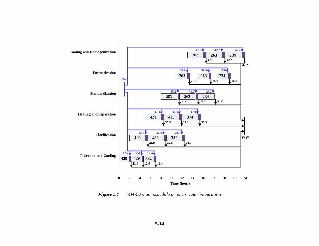
5-14
0 2 4 6 8 10 12 14 16 18 20 22 24
Filtration and Cooling
Clarification
Heating and Separation
Standardization
Pasteurization
Cooling and Homogenization
FW
WW
12.4
12.4
429 429 382
429 429 382
421 420 374
263
263
263
263
263
263 234
234
234
12.4 12.4
12.4 12.4
22.8 22.8 22.8
22.8 22.822.8
37.3 37.3 37.3
37.3 37.3
35.2
26.9
37.3
35.235.2 35.2
35.2 35.2
26.9 26.9
26.9 26.9 26.9
42.2 42.2 42.2
42.2 42.2
42.2
Time (hours)
Figure 5.7 RMRD plant schedule prior to water integration

Chapter 5 Industrial Case Study
5-15
A modification in the schedule of the RMRD is observed when comparing Figure 5.7
and Figure 5.8. The number of batches processed in the standardization,
pasteurization, and the cooling and homogenization stages was reduced from three to
two batches. The milk production was conserved by increasing the batch size while
still satisfying the maximum capacity constraint of 450 tons per batch. This then
reduced the number of washing operations required hence resulting in a decrease in
freshwater intake. The advantage of a flexible scheduling technique is also shown
when comparing both plant schedules. The start and end time of washing operations
were modified to find more water reuse opportunities in the plant as shown in Figure
5.8. However, it is worth mentioning that more batches could be fit in the first 5
processing stages to maximize the production of milk in the next 24 hours. This could
suppress some reuse opportunities around washing operations due to the restrictions
on the flexibility of the schedule. Therefore, the plant schedule proposed in Figure 5.8
can be used as a guideline for the plant to reduce its freshwater intake.
Table 5.6 gives the main components contributing to the cost of the integrated water
network and their economic value in the proposed plant setup. The unit cost of
freshwater, wastewater and, electricity was specified as 1 c.u per ton and 0.06 c.u. per
kWh respectively (Buabeng-Baidoo, et al., 2017). The capital cost of ED and storage
were calculated using the cost data specified in Table 4.4. Prior to applying the
formulation, the freshwater cost and wastewater disposal cost were the main
contributors to the total water network cost. The implementation of the proposed
technique added some additional aspect to the water network costs, i.e. capital cost of
ED and storage tanks and the electricity cost associated the energy consumption of
the regeneration process. The economic analysis shows that the reduction in
freshwater intake outweighed the additional costs associated with the exploration of
water reuse opportunities. Hence a total reduction of 20.2 % in operating costs was
achieved by implementing the proposed technique. Unlike the costs of water and
energy consumption, the capital costs are not recurring. However, as formulated in
the objective function described by Constraint (3.99), the capital costs of ED and

Chapter 5 Industrial Case Study
5-16
storage were annualized based on the equipment life which was estimated to be 5
years in this case. The revenue was not included in the costing calculations as this
will remain constant since the amount of milk and cream produced remained
unchanged after implementing the proposed technique. This then entails an increase
in the overall profit of the plant.
Table 5.6 Cost-benefit analysis of the proposed plant configuration
Current plant Proposed plant setup
Annual freshwater cost 150150 109420
Annual wastewater cost 150150 109230
Annualized ED capital cost - 528
Annualized cost of storage - 20578.2
Electricity cost - 2609.6
Total annualized cost 300300 239670.6
Percentage saving in water
network cost
19.2
The computational results obtained from the proposed optimization approach were
compared to the results of obtained from a typical black-box approach as described in
Chapter 4. Table 5.7 gives the design specifications of the water network obtained
from both approaches. The black-box approach was able to achieve a higher
reduction in freshwater consumption from the initial amount of 530.4 tons compared
to the proposed formulation. The increase in freshwater reduction was made possible
by feeding a greater amount of wastewater in the regenerator at a higher flowrate.
This explains the short duration of the regeneration process compared to the proposed
setup. The energy consumption amounted to 55.2 Wh as opposed to 2.6 Wh of energy
requirement in the proposed plant setup. Furthermore, the black-box approach

Chapter 5 Industrial Case Study
5-17
suggested a water network setup with storage capacities of 44.5 tons and 42.2 tons
each compared the capacities of 12.4 and 18.7 proposed by the developed technique.
Therefore the adoption of the proposed formulation over the black-box approach
yielded 95.2 and 10.8 decrease in energy consumption and total water network cost
respectively.
Table 5.7 Comparative study between black-box and detailed modelling
approach
Black-box
approach
Proposed formulation
Freshwater consumption (tons) 294.6 331.6
Amount of regenerated water (tons) 44.5 20.3
Duration of regeneration (h) 7.8 15.6
Total energy consumption (Wh) 55.2 2.6
Percentage energy savings - 95.2
Wastewater storage size (tons) 44.5 12.4
Diluate storage size (tons) 42.2 18.7
Total cost of water network (c.u./y) 272054 242572
Percentage savings in network cost 10.8
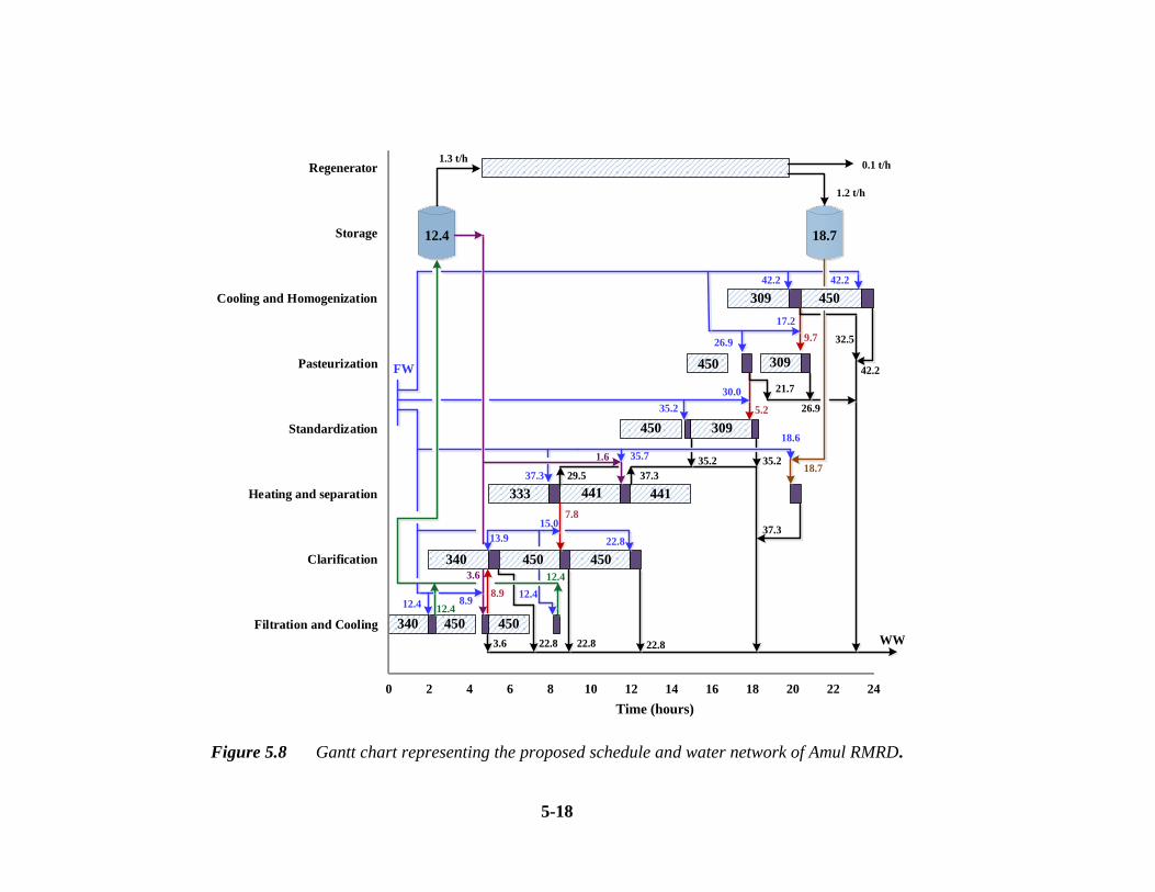
5-18
0 2 4 6 8 10 12 14 16 18 20 22 24
Filtration and Cooling
Clarification
Heating and separation
Standardization
Pasteurization
Cooling and Homogenization
Storage
Regenerator
FW
WW
340 450 450
340 450 450
333 441 441
450 309
450 309
309 450
12.4 8.912.4
13.9
15.0
22.8
37.3
35.7
18.6
35.2
30.0
26.9
17.2
42.2 42.2
12.4
12.43.6
1.618.7
8.9
7.8
5.2
9.7
3.6 22.8 22.8 22.8
29.5 37.3
37.3
35.2 35.2
21.7
26.9
32.5
42.2
1.3 t/h
1.2 t/h
0.1 t/h
12.4 18.7
Time (hours)
Figure 5.8 Gantt chart representing the proposed schedule and water network of Amul RMRD.

Chapter 5 Industrial Case Study
5-19
References
Buabeng-Baidoo, E. et al., 2017. Study of water reuse opportunities in a large-scale
milk processing plant through process integration. Chemical Engineering
Research and Design, Volume 121, pp. 81-91.
Chandan, R. C., Kilara, A. & Shah, N. P., 2016. Dairy processing and quality
assurance. 2nd ed. Chichester: John Wiley & Sons Ltd..
Memisi, N. et al., 2015. CIP cleaning processes in the dairy industry. Procedia Food
Science, Volume 5, pp. 184-186.
Tomasula, P. M. et al., 2013. Computer simulation of energy use, greenhouse gas
emissions, and process economics of the fluid milk process. Journal of Dairy
Science, 96(5), pp. 3350-3368.
Willmott, A. J., 2011. Regenerative heat exchangers. [Online]
Available at: http://www.thermopedia.com/content/1087/
[Accessed 23 May 2017].

6-1
LIMITATIONS AND
RECOMMENDATIONS
6.1 Introduction
The wastewater minimization technique developed in this work was verified and
validated against two illustrative examples. Its practicality was also tested by
applying it to a real industrial process. Several challenges were encountered during its
implementation due to the omission of some important practical considerations.
Furthermore, the structure and nature of the model influenced the computational
challenges faced as mentioned in previous chapters. This chapter highlights and
discusses the main limiting aspects of the proposed formulation and elaborates on
possible avenues of future improvement.
6.2 Water network limitations
6.2.1 Single contaminant
The proposed formulation was developed for wastewater minimization problems with
a single key contaminant. This entails that all existing water streams were
characterized by one common contaminant. This assumption has proven to reduce the
complexity of the resultant model at the expense of reducing its practicability in the
6

Chapter 6 Limitations and Recommendations
6-2
process industry. Wastewater streams with multiple contaminants are more prevalent
to industrial water networks as compared to single contaminant. This is many due to
the fact that tasks involved in a typical batch production scheme are inherently
different. Therefore, it is of utmost importance for this work to be adapted to multiple
contaminant problems for a possible increase in its industrial applications.
6.2.2 Water-using operations
The batch water network was optimized in this work by exploring reuse opportunities
between various washing operations. Washing operations are typical examples of
mass transfer processes. A mass transfer operation entails the transfer of
contaminants from a rich stream, i.e. a stream with higher contaminant concentration,
to a lean stream, i.e. a stream with lower contaminant concentration. In the case of
washing operations, processes are considered as rich streams and water streams used
to clean these processes are lean streams. Another example of a mass transfer-based
mechanism is the solvent extraction process. However, there can be instances where a
process itself produces water as a by-product or consumes water as a feedstock or
reactant. These types of processes are called non-mass transfer processes and cannot
be modelled using Constraints (3.3) and (3.5) as presented in Chapter 3. In the event
where non-mass transfer processes are large contributors to the freshwater
consumption or wastewater generation of a batch process, the abovementioned
constraints will be omitted in their mathematical representation. Constraint (3.1) and
(3.2) will then be used interchangeably depending on the type of non-mass transfer
process involved in the water network.
6.2.3 Water treatment technology
The quality of industrial wastewater effluents is usually measured by their physical,
chemical and biological composition. The major constituents of concern in
wastewater treatment for reuse or disposal are the suspended solids, dissolved
inorganics, heavy metals, nutrients, pathogens, biodegradable and refractory organics

Chapter 6 Limitations and Recommendations
6-3
(Tchobanoglous, et al., 2003). Several indices are used as collective measures of
those components and this includes the Total Suspended Solids (TSS), Total
Dissolved Solids (TDS), Chemical Oxygen Demand (COD), Biological Oxygen
Demand (BOD), etc. The water network embedded an electrodialysis (ED) treatment
unit to partially purify wastewater effluents and facilitate their reuse within the
process. The advantage of ED relies on its ability to efficiently purify effluents
without requiring intense pre-treatment, relatively easy cleaning procedure and can
even be self-cleaned through electrodialysis Reversal (EDR) (Chao & Liang, 2008). It
is also suitable for intermittent systems such as batch systems due to its relatively
simple start up and shut down procedure (Strathmann, 2004).However, ED is limited
to the removal of ionic compounds in wastewater. This then suppresses its
applicability to a typical industrial water network with multiple contaminants.
The extension of this formulation to a wider range and variety of contaminants will
require an enhancement of the wastewater system. This entails adapting the
formulation to multi-contaminants water systems by having a network of wastewater
treatment technologies in the problem superstructure. For Instance, in the industrial
case study presented in Chapter 5, the quality of wastewater effluents was measured
by their concentration in total dissolved solids (TDS) to facilitate the treatment
though ED. However, wastewater from dairy processes contains various other
contaminants such as TSS and biodegradable organics measured by the COD or
BOD. The network could consist of a combination of many other technologies such
as Reverse Osmosis (RO), Nanofiltration (NF) and Ultrafiltration (UF) which can be
configured in series or parallel. Since each technology has its own contaminant
selectivity, this would allow the model to then select the type of technology suitable
for the treatment of effluents generated within a given batch water network
In this formulation, a preliminary design of the ED process was performed to mainly
determine the size of the stack, the total membrane area required and the total
consumption of energy. The contaminant removal rate of the ED process was defined

Chapter 6 Limitations and Recommendations
6-4
as a parameter during optimization. Future work should enhance the ED design by
providing more details with regards to the type and properties of membranes and
design of spacers. Spacers are placed between membranes to ensure uniform flow in
each ED cell, maximize mixing of solutions at the surface of membranes and
minimize pressure loss. The type of spacers is also a key determiner of the flow path
through the ED stack (Strathmann, 2004). It is also advisable to explore the case
where the contaminant removal rate is determined through optimization. However,
this could drastically increase the CPU time hence alternative optimization routes will
be discussed later in this chapter.
6.3 Scheduling considerations
The schedule of a batch plant is a key aspect in the optimization of its water network.
The discrete occurrence of water using operations within a given production scheme
showed the importance of an adequate plant scheduling. This has allowed for more
water reuse opportunities to be obtained since the optimization of the plant schedule
and batch water network were performed simultaneously as mentioned in Chapter 4
and 5. The scheduling model adopted in this work was mainly formulated for
multipurpose batch plants. The main scheduling decisions that were made were the
allocation of tasks to units, batch sizing, and sequencing decisions. However, in
practice, the level of decision making in production scheduling may vary from one
plant to the other depending on the decisions made by the higher management. This is
mainly due to the fact that the scheduling task forms an integral part of a supply chain
management and interactions between various functions is plant specific. For
instance, if the decision of batch sizing is made at the planning level, then scheduling
will be reduced to only assigning tasks to units and determining the optimum
sequences of tasks (Harjunkoski, et al., 2014). Therefore, the scheduling model
adopted in this formulation should be adapted to the production environment of
particular a plant for a successful implementation.

Chapter 6 Limitations and Recommendations
6-5
This formulation considered a short-term scheduling of batch processes. This implies
that the makespan within which batch tasks occur is limited to few hours or days. In
fact, the highest time horizon considered in the presented case study and illustrative
examples was 24 hours. Since the presented results are primarily dependent on the
length of the makespan, the short-term scheduling consideration is a major limitation
of the presented work. A longer time horizon would have tremendous impact on the
batch production schedule and the water network design. It could incur changes in the
design specifications of the electrodialysis process, the resultant sizes of storage and
the reuse opportunities found around batch operations.
In order for this formulation to be applicable to medium and long-term scheduling
problems, additional scheduling aspects such as cyclic production and scheduling
under uncertainties will have to be considered. The concept of cyclic scheduling
involves the incorporation of short-term scheduling concepts in long time horizons. It
considers the repetition of an optimum schedule obtained within a short time horizon
when the problem is extended to longer horizons (Nonyane & Majozi, 2011). This
will then result in many cycles of the same sequence of tasks and allow the reuse of
water streams from one cycle to the other through the use of storage vessels.
However, the assumption of constant production schedule from one cycle to the other
might prove to be unrealistic in market demands characterized by frequent variation
in product demand. In this case, rescheduling of tasks will be required when sudden
changes occur in production requirements as specified through demand forecasting
(Harjunkoski, et al., 2014).
6.4 Computational intensity
Table 4.5, 4.10 and 5.4 previously discussed in Chapter 4 and 5 gives data showing
the computational intensity of the proposed formulation. The results for both
illustrative examples and the industrial case study were obtained in a high
computational time of approximately 8 hours. The Challenge with high CPU time

Chapter 6 Limitations and Recommendations
6-6
arises when for instance rescheduling of a given batch plant is performed on a regular
basis for production improvement or water network optimization. In this case,
mathematical models with high computational burden will not be attractive to the
industry. However, it is worth mentioning that the presented formulation involves the
design of equipment such as regenerator and storage tanks and constraints used to
describe those units mainly contributed to the computational burden. In the event
where a wastewater regeneration unit and storage tanks are readily available within
the plant, the problem formulation will be drastically simplified and the CPU time
will be reduced. At a design level, a large CPU time is less problematic since no
operation is being undertaken and the focus is on providing an optimum design of the
plant. Nevertheless, it is important to discuss possible ways to improve the
computational time and some will be elaborated in this section.
6.4.1 CPU time improvement
The computational expensiveness of the proposed formulation is mainly due to its
structure and size. The statistics of the resultant models for all examples, as presented
in Tables 4.5, 4.10 and 5.4, show that the formulations yielded large scale models
with the number of constraints and variables ranging from 5200 to 6900 and 1600 to
2280 respectively. The nonlinearity and nonconvexity of the proposed formulation
are other key aspects contributing to computational difficulties. Methods of CPU time
reduction which might prove to be effective include convexification and pre-
processing techniques. The type of solver, on the other hand, can contribute to the
increase in computational time depending on the structure of the model. Pre-
processing techniques are other ways in which the solution time can be improved in
future work. These aspects are discussed and examined below.
(a) Convexification techniques
The use of convexification techniques is among the possible ways in which the CPU
time of a MINLP problem can be reduced. This includes the Glover transformation,
Chapter 6 Limitations and Recommendations
6-7
the McCormick (1976) and Lundell et al. (2013) reformulation techniques discussed
in Section 2.2.4 of Chapter 2. It is worth mentioning that Glover transformation has
been applied to the existing model to linearize the bilinear term pyp rere found in
Constraint 3.80 which defines the duration of the regeneration process. The
McCormick estimation could be used to relax all bilinear terms found in most water
balance constraints. The solution to the relaxed formulation could then be used as
starting point in the exact MINLP problem. However, in the event where upper and
lower bounds of variables are unknown or too large, this approach could result in an
increase in CPU time due to the enlargement of the search space. The convexification
techniques applied to the SGO algorithm of Lundell et al. (2013) can be also be used
to reformulate bilinear terms and other signomial functions found in the formulation.
This could provide tighter convex regions for bilinear terms depending on the value
of the parameter α.
(b) Optimization solver
The Branch and Reduce Optimization Navigator (BARON) was the chosen
optimization in this work to yield global optimal solutions for the presented case
studies. As discussed in Section 2.2.5 of Chapter 2, BARON uses a LP-based branch
and bound based algorithm which annexes duality techniques to reduce the size of the
model during the solution process. Its robustness lies in its ability to solve a wide
range of optimization problems and handle various nonlinear functions. Its solution
algorithm can often guarantee global solutions of nonconvex problems and does not
require initialization of variables (Sahinidis, 2014). However, the major challenge
encountered with BARON 14.0.3 was the use large number of nodes between two
optimal points during its search for the global optimal value. Hence, the solution
procedure was terminated by limiting the computational time to a certain extent at the
expense of stopping at a local optimal point.

Chapter 6 Limitations and Recommendations
6-8
During online process optimization, i.e. optimization performed during plant
operation, the main goal is to determine key variables which have a major effect on
the objective function and providing improved plant performance in minimum CPU
time. Global optimality becomes of greater essence when plant design is still being
undertaken. Marginal values in mathematical programming tell the modeller the
extent to which all variables affect the objective function. This further allows the
determination of critical variables, i.e. variables which should be manipulated by the
process engineer to get greater saving in water for instance or greater improvement in
plant profit. However, BARON 14.0.3 did not provide marginal values for the models
solved in this work. Hence such information could not be provided which forms
another limitation of this work.
The performance of BARON 14.0.3 could be improved by revisiting of the proposed
formulation, tightening or adding bounds on certain variables and exploring possible
ways of further reduction in model size. This entails removing redundant constraints
if existent or reducing the number of both continuous and binary variables by
reformulating some constraints in the model. Scaling of variables could also be useful
to reduce the CPU time by ensuring that the magnitudes of variables are within the
same order (GAMS Development Corp., 2014). It is worth pointing out that the
features of BARON solver have been enhanced in its latest version, i.e. BARON
17.4.1. For instance, BARON 17.4.1 allows its MIP subsolver to use multiple cores
simultaneously to decrease the CPU time since most of the solution time is spent on
solving MIP relaxations. The use of multiple cores is translated into the simultaneous
use of multiple processors amenable to parallel computing (Sahinidis, 2017).
Furthermore, some other MINLP solvers discussed in Chapter 2 should be tested on
the presented formulation to assess their efficacy compared to BARON. DICOPT,
for instance, allows the user to choose MIP and NLP solvers that will give the best
computational performance for a given model. NLP solvers used in DICOPT often
requires the initialization of variables involved in nonlinear terms which, if

Chapter 6 Limitations and Recommendations
6-9
adequately chosen, can drastically reduce CPU time for large scale problems (GAMS
Development Corp., 2014).
(c) Pre-processing techniques
Pre-processing techniques are usually built-in functions in many MINLP solvers.
They aim to improve a given formulation by analysing each constraint, identify any
infeasibility or redundancy and improve bounds to reduce the optimization search
space (Savelsbergh, 1994). Additional pre-processing can also be applied to the
model prior to attempting to solve it in order to reduce the computational time. For
instance, a graphical targeting technique could be used as a pre-processing step for
the proposed formulation to determine the optimum value of some variables such as
the removal ratio of the ED process without increasing the computational burden. The
resultant water network from graphical targeting can also be used as a starting point
for mathematical optimization to reduce the CPU time.
(d) Design model of the electrodialysis process
The complexity of the electrodialysis design sub-model is a major contributor the
high CPU time of the proposed formulation. In published literature, researchers have
opted for black-box approaches to model regeneration units due to their simplicity.
Blackbox models are usually made of linear equations, hence they can greatly
contribute to the reduction of the CPU time. However, the CPU time is usually
reduced at the expense of losing accuracy on the costing of the water network. It is
worth reiterating that the merit of the proposed formulation resides in its ability to
provide the modeller with the optimum sizes of the regenerator while enabling the
minimization of its energy consumption. Blackbox approaches, on the other hand,
focus on optimizing the cost of regeneration by manipulation performance indices
such as feed flowrate and removal ratio. This usually results in an underestimated
overall cost of the regeneration process. It is therefore recommended to find a middle
way between black-box and detailed modelling approaches as a strategy for CPU

Chapter 6 Limitations and Recommendations
6-10
time improvement. In other words, the development of a simplified ED can design
model which has the ability to capture the merits of both modelling strategies should
be the subject of future research studies.
References
Chao, Y.-M. & Liang, T. M., 2008. A feasibility study of industrial wastewater
recovery using electrodialysis reversal. Desalination, Volume 221, pp. 433-439.
GAMS Development Corp., 2014. GAMS - The Solver Manuals, Washington DC:
s.n.
Harjunkoski, I. et al., 2014. Scope for industrial applications of production scheduling
models and solution methods. Computers and Chemical Engineering, Volume
62, pp. 191-193.
Lundell, A., Skjal, A. & Westerlund, T., 2013. A reformulation framework for global
optimization. Journal of Global Optimisation, Volume 57, pp. 115-141.
McCormick, G. P., 1976. Computability of global solutions to factorable nonconvex
programs: Part I - Convex underestimating problems. Mathematical
Programming, Volume 10, pp. 147-175.
Nonyane, D. R. & Majozi, T., 2011. Long term scheduling technique for wastewater
minimization in multipurpose batch processes. Applied Mathematical Modelling.
Sahinidis, N., 2014. BARON, s.l.: The Optimization Firm.
Sahinidis, N., 2017. BARON user manual v. 17.4.1, s.l.: The Optimization Firm.
Savelsbergh, M. W. P., 1994. Preprocessing and Probing techniques for mixed
integer programming problems. ORSA Journal on Computing, 6(4), pp. 445-454.
Silva, V., Poiesz, E. & van der Heijden, P., 2013. Industrial wastewater desalination
using electrodialysis: evaluation and plant design. J Appl Electrochem, Volume
43, pp. 1057-1067.
Strathmann, H., 2004. Assessment of electrodialysis for water desalination process
costs, Limassol: Institute of Chemical Engineering, University of Stuffgart,
Germany.
Tawarmalani, M. & Sahinidis, N. V., 2005. A polyhedral branch-and-cut approach to
global optimization. Mathematical Programming, 103(2), pp. 225-249.
7-1
CONCLUDING REMARKS
The work presented in this dissertation focused on developing a mathematical
formulation for the minimization of freshwater use in batch water networks with a
single key contaminant. The water network comprised washing operations, a buffer
system with two storage tanks and an embedded regeneration system. The technique
considered short-term scheduling of batch plants which forms the platform for the
synthesis of the water network. The simultaneous optimization of scheduling and
water use yielded the optimum schedule that is concomitant with the minimum
freshwater usage. The regenerator system was designed with sufficient details to
enable the determination of its size and quantification of its energy consumption,
allowing an accurate costing of the water network.
The formulation was validated using two illustrative examples and an industrial
process. In all cases, the formulation yielded large-scale MINLP models. A reduction
in freshwater intake of 37 % and 41 % were respectively achieved in both industrial
examples while maintaining a maximum production. The schedule of each plant was
generated and details on the batch size and the optimum sequences of tasks were
given for each processing unit. The design specifications of the ED treatment units
and their optimum consumption of energy were also obtained. The industrial case
study aimed to test the practicality of the developed formulation by exploring reuse
7

Chapter 7 Concluding remarks
7-2
opportunities in the RMRD section of Amul, a dairy based in India. The freshwater
usage was reduced by 37 % and a modified plant schedule was suggested. An
economic analysis was performed on the optimized plant and a reduction in operating
cost of 20 % was observed.
The presented technique is limited to single contaminant cases which are very seldom
in the process industry and the regeneration system only allows the removal of ionic
contaminants through electrodialysis. Furthermore, optimum solutions are generated
in a considerably high CPU time. It is therefore recommended that future work
focuses on extending this formulation to account for multiple contaminants and
medium to long-term scheduling which involves cyclic production. An enhancement
of regeneration system is also required to include a network of distinct wastewater
treatment technologies and facilitate the removal of various contaminants. Although
the current work focusses on the usage of water as a mass separating agent (MSA), it
can be readily adjusted to cater for both mass transfer and non-mass transfer-based
operations. A substantial effort should be directed towards reducing the
computational time of optimization solvers by adopting pre-processing and relaxation
techniques that alleviate the complexity of the proposed formulation. Nonetheless,
this work provides a solid basis for future research to develop improved wastewater
minimization techniques for multipurpose batch plants.

A-1
Appendices
Appendix A: Scheduling formulation of Seid and Majozi
(2012)
The scheduling model of Seid and Majozi (2012) is based on the SSN representation
of Majozi and Zhu (2001). It was developed for multipurpose batch plants aiming at
maximizing the profit of the plant or minimizing the makespan and obtain a plant
schedule with an optimized utilization of resources. The following data need to be
known prior to optimization.
(i) The production recipe which indicate the sequence of tasks for the conversion
of raw materials into products
(ii) The capacity of each unit, the type and number of task each unit can process.
(iii)The maximum storage capacity of all materials
(iv) The time horizon of interest
The mathematical formulation includes the following constraints.
A.1 Allocation constraint
Constraint (A.1) states that only one task can be active in a unit at any given time slot
p.
*
,
1,
jininj Ss
in
j psy PpJj , (A.1)

Appendix A Scheduling formulation of Seid and Majozi
A-2
A.2 Capacity constraint
Constraint (A.2) ensures that the amount of batch processed in a unit at any given slot
p does not exceed the capacity of the unit. L
sinj
V and U
s inj
V represents the lower and upper
capacity limits for the batch size of a given material statein
js .
psyVpsmpsyV in
j
U
s
in
ju
in
j
L
s inj
inj
,,, in
j
in
j SsPpJj ,, (A.2)
A.3 Material balance for storage
Constraint (A.3) states that the amount of material s stored at any slot p is as the
amount that was previously stored at slot p-1 adjusted to an amount resulting from the
difference between the portion of state s produced at slot p-1 and the portion used at
the current slot p. Constraint (A.4) represents the storage balance for product sp. It
ensures that, at any given slot p, the amount of product produced adds up to the
amount that was present in storage at slot p-1 to give the total amount of product
stored at time slot p.
sp
jininj
inj
scjin
inj
inj
Ss
in
ju
sp
s
in
j
Ss
u
sc
sss psmpsmpsqpsq
,,
1,,1,,
PpSs ,
(A.3)
ps
jininj
inj
Ss
in
ju
sp
s
p
s
p
s psmpsqpsq
,
,1,,
pp Ss,Pp
(A.4)
A.4 Duration constraint: Duration as a function of batch size
The duration of a task in a particular processing unit is given by Constraint (A.5). It
is defined as the time difference between its starting and finishing time and is
dependent on the batch size.

Appendix A Scheduling formulation of Seid and Majozi
A-3
psmspsyspstpst in
ju
in
j
in
j
in
j
in
ju
in
jp ,,,,
in
j
in
j SsPpJj ,, (A.5)
A.5 Sequence constraints
A.5.1 Same task in the same unit
Constraint (A.6) ensures that a batch starts being processed in a unit at slot p after the
completion of the previous batch in the same unit at the previous time slot p-1. In this
case, both batches are of the same nature, i.e. they are made of the same material
state.
1 p,stp,st injp
inju
*j,in
inj Ss,Pp,Jj (A.6)
A.5.2 Different tasks in the same unit
Similar to Constraint (A.6), Constraint (A.7) ensures that a task start being processed
in a unit after all the previous tasks are completed. This constraint looks at a case
were different tasks can occur in the same unit.
1,, ' pstpst in
jp
in
ju *
,
'' ,,,, jin
in
j
in
j
in
j
in
j SssssPpJj (A.7)
A.5.3 Different tasks in different units
(a) If an intermediate state is produced from one unit
Constraint (A.8) ensures that an intermediate state produced in a unit does not exceed
its storage capacity if it is produced at time slot p-1 but not consumed in another unit
at time slot p, i.e. t(j,p)=0. If both the producing and consuming task are active at
consecutive time slots, then the amount of intermediate state stored will be less than

Appendix A Scheduling formulation of Seid and Majozi
A-4
the amount produced. The binary variable t(j,p) will then takes a value of 1 and
Constraint (A.9) will hold. Constraint (A.9) ensures that the consuming task of an
intermediate state start after the completion of its producing task.
pjtVpsqpsm U
js
in
ju
sp
s inj
,,1,
sp
jin
in
j SsPpJj ,,, (A.8)
pjtpsyHpstpst in
j
in
jp
in
ju ,1,21,,'
sc
jin
in
j
sp
jin
in
j SsSsPpJj ,', ,,, (A.9)
(b) If an intermediate state is produced from more than one unit
Constraint (A.10) states that the amount of state consumed by a task can either come
from storage or directly from its producing units. Depending whether t(j,p)=0 or
t(j,p)=1 as explained earlier, Constraint (A.9) will also be used for sequencing in this
category. Constraint (A.11) ensures that the starting time of a task consuming an
intermediate state occurs after the completion of all the producing tasks which
occurred at pervious time slots. This constraint ensures adequate sequencing between
non-consecutive tasks consuming and producing an intermediate material. In this
case, the producing task occurred at slot p-2 and the consuming task is occurring at
the current slot p.
sp
jininj
inj
scjin
inj
inj
Ss
in
ju
sp
ss
Ss
in
ju
sc
spjtpsmpsqpsm
,,
,1,1,,
PpJj , (A.10)
2,12,,' psyHpstpst in
j
in
jp
in
ju
sc
jin
in
j
sp
jin
in
j SsSsPpJj ,', ,,, (A.11)
Appendix A Scheduling formulation of Seid and Majozi
A-5
A.6 Sequence constraints for FIS policy
Constraint (A.12) ensures that the amount of intermediate state stored at any point in
time does not exceed the available storage capacity. The binary variable x(s,p)
indicates the availability (x(s,p)=1) or absence of storage (x(s,p)=0) for intermediate
sate s at time slot p. Constraint (A.13) states that the finishing time of the producing
task should coincide with the starting time of the consuming task of state s provided
that no storage is available for this state, i.e. x(s,p)=0. This constraint is relaxed if
there is an available storage for intermediate state s, i.e. x(s,p)=1.
s
spjin
inj
inj
Jj
U
j
U
s
Ss
in
ju
sp
spsxVQSpsqpsm ,11,1,
,
SsPpJj ,, (A.12)
psxHpsypsyHpstpst in
j
in
j
in
jp
in
ju ,1,,21,, ''
SsSsSsPpJj sc
jin
in
j
sp
jin
in
j ,,,, ,', (A.13)
A.7 Storage constraints
Constraint ((A.14) indicates that the amount of state s stored should not exceed the
maximum capacity of the available storage. The storage capacity for state s in this
case includes the capacity of both its dedicated storage tank and its producing units.
Constraint ((A.15) ensures that intermediate materials are stored in their producing
units at consecutive time slots. Constraint ((A.16) ensures that a unit being utilized
for a temporary storage of an intermediate material at time slot p is not assigned to
process any task at that time slot.
sp
jininj Ss
in
j
U
s psuQSpsq
,
,, SsPpJj ,, (A.14)
1,1,, psupsmpsu in
j
in
ju
sp
s
in
j inj
sp
jin
in
j SsPpJj ,,, (A.15)

Appendix A Scheduling formulation of Seid and Majozi
A-6
*,
,1,
jininj Ss
in
j
U
j
in
j psyVpsu sp
jin
in
j SsPpJj ,,, (A.16)
A.8 Tightening constraints
Constraint (A.17) is used to ensure that all tasks processed by a given unit occur
within the time horizon. It states that the sum of the duration of all tasks processed in
a unit should not exceed the length of the time horizon. For the purpose of this work,
Constraint (A.17) was modified into Constraint (A.18) to also cater for the duration
of washing operations in the tightening constraints. This is due to the fact that a
washing operation is scheduled to occur after a batch task has been completed.
Hpsmpspsyps
jininj Ss p
in
ju
in
j
in
j
in
j *
,
,,,,
Jj
(A.17)
Hpsmps
psypspsyps
jininj Ss p
in
ju
in
j
in
j
in
j
win
j
in
j
*
,,,
,,,,
Jj
(A.18)
A.9 Time horizon constraints
Constraint ((A.19) and ((A.20) ensures that the starting and finishing time of all the
tasks occur within the time horizon of interest
Hpst in
ju , in
j
in
j SsPpJj ,, (A.19)
Hpst in
jp , in
j
in
j SsPpJj ,, (A.20)

Appendix A Scheduling formulation of Seid and Majozi
A-7
A.10 Nomenclature
The following sets, parameters and variables are used in the scheduling formulation
of Seid and Majozi (2012).
Sets
P { p|p represents a time point}
J { j|j denotes a unit}
S { s|s represent any state other than a product}
PS {PP s|s represent any state other than a product}
injS { in
jinj s|s is an effective state representing a task performed in
unit j}
scj,inS { sc
j,insc
j,in s|s task which consumes state s}
*j,inS { *
j,in*
j,in s|s task performed in unit j}
spj,inS {
spj,in
spj,in s|s task which produce a state s other than a product}
PSj,inS {
PP Sj,in
Sj,in s|s task producing a state which is a product}
Parameters
UjV capacity of unit j
U
s inj
V maximum capacity of unit j to process a task
L
s inj
V minimum capacity of unit j to process a task
H time horizon of interest
oQS initial amount of state s found in storage

Appendix A Scheduling formulation of Seid and Majozi
A-8
UQS maximum storage capacity for state s
injs duration of a processing task in unit j
injs duration of a processing task in unit j
inj
w s duration of washing in unit j
spj,ins portion of state s produced by a task
scj,ins portion of state s consumed by a task
Variables
p,smu inj amount of material processed by a task at time slot p
p,su inj amount of material stored in unit j at time slot p
p,st inj
u starting time of a task at time slot p
p,st inj
p finishing time of a task at time slot p
p,sy inj binary variable associated with the assignment of a task at time
slot p
p,sx binary variable associated with the availability of storage
assignment of a task at time slot p
p,sqS amount of state s stored at time slot p binary variable
associated with the assignment of a task at time slot p
p,jt binary variable associated with the usage of a state produced
by unit j at time slot p
References
Majozi, T. & Zhu, X. X., 2001. A novel continuous time MILP formulation for
multipurpose batch plants. 1. Short-term scheduling. Computer Aided Chemical
Engineering, Volume 9, pp. 937-942.
Seid, R. & Majozi, T., 2012. A robust mathematical formulation for multipurpose
batch plants. Chem. Eng. Sci., Volume 68, pp. 36-53.


