Research Collection

Doctoral Thesis

Conceptual models of single and multiphase transport in afracture

Author(s): Lunati, Ivan Fabrizio

Publication Date: 2003

Permanent Link: https://doi.org/10.3929/ethz-a-004563030

Rights / License: In Copyright - Non-Commercial Use Permitted

This page was generated automatically upon download from the ETH Zurich Research Collection. For moreinformation please consult the Terms of use.

ETH Library

Diss. ETH No.: 15082

Conceptual Models of Single andMultiphase Transport in a Fracture

A dissertation submitted to theSwiss Federal Institute of Technology Zürich

for the degree ofDoctor of Natural Sciences

presented by

Ivan Fabrizio Lunati

Dipl.-Phys.University of Milan, Italyborn on January 17, 1973

citizen of Italy

Accepted on recommendation of

Prof. Dr. Wolfgang Kinzelbach, examinerProf. Dr. Hannes Flühler, co-examiner

Zurich, 2003

i

En la realidad el número de sorteo es infinito.Ninguna decisión es final, todas se ramifican en otras.

J.L.Borges, Ficciones

ii

iii

Table of Contents

Table of contents…………………………………………………………………... iii

Abstract………………………………………………………………………….… v

Estratto…………………………………………………………………………….. vii

1 Introduction……………………………………………………………………… 1

2 Macrodispersivity for transport in arbitrary non-uniform flow fields:Asymptotic and Pre-asymptotic results…………………………………...…… 7

2.0 Abstract……………………………………………………………………… 7

2.1 Introduction………………………………………………………………….. 9

2.2 Statement of the problem……………………………………………………. 10

2.2.1 Two-scale functions……………………………………………………. 11

2.2.2 The dimensionless transport equation and the time scales…………….. 12

2. 3 Two-scale analysis of the transport equation………………………....……. 14

2.4 Asymptotic macrodispersivity in porous media (wide scale separation)…… 17

2.4.1 Homogenization of the flow problem………………………………….. 17

2.4.2 Homogenization of the transport equation in porous media………….... 19

2.4.3 An explicit result: macro dispersivity in lowest order perturbationtheory……………………………………...………………………….... 20

2.5 Extension to pre-asymptotic transport behaviour…………………………... 24

2.6 Summary and conclusions………………………………………………….. 28

2.7 Appendix A…………………………………………………………………. 29

3 Effects of pore volume-transmissivity correlation on transport phenomena.. 31

3.0 Abstract……………………………………………………………………... 31

3.1 Introduction…………………………………………………………………. 33

3.2 Experimental observations………………………………………………….. 34

3.2.1 Experimental procedure: the empty fractures…………………………. 35

3.2.2 Experimental procedure: the filled fractures………………………….. 37

3.3 Theoretical discussion……………………………………………………… 38

3.4 A numerical case study: dipole in a closed box……………………………. 40

3.4.1 The T−φ correlation models…………………………………………. 42

3.4.2 Numerical results……………………………………………………… 45

3.5 Conclusions………………………………………………………………… 53

iv

4 Water soluble gases as partitioning tracer to investigate the pore volume-transmissivity correlation in a single fracture………………………………… 55

4.0 Abstract……………………………………………………………………… 55

4.1 Introduction………………………………………………………….………. 57

4.2 Theoretical background of a Gas Tracer Test ……………………………… 58

4.2.1 Two phase flow and gas migration…………………………………….. 59

4.2.2 Multi-component transport and inter-phase mass transfer…………….. 60

4.3 Pore volume-transmissivity correlation models…………………………….. 62

4.4 Numerical simulations of a Gas Tracer Tests in a heterogeneous singlefracture……………………………………………………………………… 63

4.4.1 Low-variance transmissivity fields……………………………………. 67

4.4.2 High-variance transmissivity fields……………………………….…… 73

4.5 Conclusions…………………………………………………….…………… 78

4.6 Appendix B…………………………………………………….…………… 80

4.7 Appendix C……………………………………………………….………… 81

5 Two-phase flow visualization in a single fracture by Neutron Radiography. 835.0 Abstract………………………………………………………….….……….. 83

5.1 Introduction……………………………………………………….….……… 85

5.2 Neutron Radiography: Theoretical background and technology……..……... 86

5.3 The fracture sample…………………………………………….…….……... 88

5.3.1 Core drilling………………………………………………….….……... 88

5.3.2 Preliminary non-invasive investigation by x-ray CT scan….….………. 88

5.3.3 Core processing……………………………………………….….…….. 89

5.4 Experimental procedure…………………………………………….….……. 92

5.4.1 Capillary imbibition….……………………………………….….…….. 92

5.4.2 Water displacement by air injection………………………….….…….. 96

5.5 Conclusions…………………………………………………………..……... 98

6 Synthesis and conclusions…………………………………………….….…….. 99

References…………………………………………………………………….…... 103

Acknowledgement…………………………………………………………….…... 107

Curriculum Vitae…………………………………………………………….…… 109

v

Abstract

Understanding flow and transport in fractured rocks is of primary importance for riskassessment of nuclear-waste repositories. Indeed, long-term disposals of nuclear wasteare mostly foreseen in low-permeability rocks, in which fractures represent preferentialflow paths through which the contaminants might come out and reach the biospherewith potential health and environmental hazard. Since fractures have a multi-scalevariability that cannot be explicitly described by any model and since large-scale(kilometer) long-term (thousand of years) predictions are needed, whereas experimentsare performed at the meter and day scale, upscaling of transport is an important issue.

We homogenize the transport equation in an arbitrary mean velocity field. First weshow that small-scale variability of the velocity field can be incorporated in amacrodispersive term, if small and large scales are widely separated. If the flow isDarcian and small-scale dispersion is negligible, we demonstrate that macrodispersivityis a medium property. Then we heuristically extend our analysis to a finite separationbetween scales and we show that standard ensemble averaging does not consistentlyaccount for finite scale effects: it tends to overestimate the dispersion coefficient in thesingle realization.

When modelling a fracture we have to make several hypotheses on its internal structureand assume relationships among different properties of the medium in order to be ableto build a physically based model of the system. In other words we have to assume aconceptual model, which guides us in making assumptions over the processes that takeplace in the system.

Following the criterion that a model has to be as simple as possible, we focus ourattention on three different types of fracture, which correspond to very intuitive andsimplified models: a rough-walled fracture filled with a homogeneous fault-gouge, anempty fracture and a parallel-plate fracture filled with a heterogeneous fault-gouge.These three models naturally imply a different relationship between transmissivity fieldand pore space (thickness-porosity): in the parallel plate model they are uncorrelated,whereas in the rough-walled filled fracture they are perfectly correlated. These twosituations represent two extremes between which the empty fracture is an intermediatesituation.

Experimental observations in rough-walled plexiglass fractures show that the presenceof a homogeneous fault gouge drastically changes the behaviour of the tracer: thepropagating front appears much smoother when the fracture is filled with glass beadsthan when it is empty. By numerical simulations in hydraulically equivalent models, wedemonstrate that the correlation between pore volume and transmissivity yields a muchsmoother and more homogeneous solute distribution. If perfect, the pore volume-transmissivity correlation makes the pore velocity depend only on the hydraulic gradientas in a homogeneous medium.

When considering two-phase flow, differences between the conceptual models, as wellas between high and low-transmissivity regions within the same fracture, are enhancedby the non-linearity of the governing equations. As we assume Leverett’s model,transmissivity and pore volume fields that are not correlated to each other imply a spacedependent entry pressure such that the gas-phase is unevenly distributed and the

vi

streamlines collapse into few channels characterized by high gas saturation andseparated by water-saturated regions. In contrast, entry pressure becomes constant inspace, when the pore volume-transmissivity correlation is perfect (homogeneous faultgouge), and yields a smoother gas-phase distribution.

These striking differences pose the problem of discrimination and identification of theadequate conceptual model, which properly describes solute concentration or gas-phasedistribution in the fracture. We demonstrate that traditional tracer tests are inadequate toinvestigate the fracture properties and discriminate among conceptual models. This hasa very simple and obvious reason: breakthrough curves at the extraction borehole sufferan information loss from averaging over different streamlines.

Gas tracer tests performed in a fracture partially desaturated by gas injection, investigatethe large-pore part of the fracture because of the effects of capillary pressure at themicroscopic scale. We show that gas tracer tests are also inadequate to discriminatebetween conceptual models if a single gas tracer is used. This is again due to theinherent nature of the breakthrough curves, which suffer from averaging over differentstreamlines.

A more promising way to improve information is to employ two or more tracers thathave different water solubility. The gas tracers behave like partitioning tracers anddissolve in the water phase according to their solubility and the amount of wateravailable. By comparing the residence-time distributions of two tracers we can computea streamline retardation, from which we can extrapolate a streamline effectivesaturation. We demonstrate by numerical simulations that this technique provides anexcellent tool to estimate the saturation of the fracture. Moreover, the streamlineeffective saturation curve contains important information, which is useful todiscriminate among conceptual models.

Finally, we consider the possibility of integrating information from breakthrough curveswith laboratory experiments. We use neutron tomography to visualize imbibition anddrainage in a core from a fault-gouge filled fracture. By comparison of tomographicimages of the sample before and after imbibition, as well as before and after drainage byair injection, we observed an uneven water distribution at the centimeter scale. Thisshows that the air phase is very irregularly distributed, indicating air flow throughpreferential paths.

vii

Estratto

Per la valutazione del rischio connesso allo smaltimento delle scorie radioattive èimportante comprendere il flusso idraulico ed il trasporto di inquinanti nei mezzifratturati. Infatti molti depositi per scorie radioattive sono progettati in roccecaratterizzate da un bassa conducibilità idraulica nelle quali le fratture costituiscono uncammino preferenziale per le sostanze inquinanti, che possono fuoriuscire ed entrare incontatto con la biosfera, dove rappresentano un pericolo per la salute e l’ambiente.

Per la corretta valutazione del rischio, sono necessarie previsioni su larga scala(chilometri) ed a lungo termine (migliaia di anni), mentre gli esperimenti sonocomunemente condotti a scale spaziali dell’ordine del metro e nell’arco temporale diqualche giorno. Inoltre, l’eterogeneità delle fratture ha una variabilità a diverse scale chenon può essere descritta esplicitamente in alcun modello. Risolvere il problemadell’upscaling per i parametri dell’equazione del trasporto è quindi fondamentale perottenre delle previsioni affidabili. La Teoria dell’Omogeneizzazione è qui applicata adun campo di velocità di valor medio arbitrario. Nel caso in cui la scala spazialedell’eterogeneità sia infinitamente più piccola della scala del modello, dimostriamo chele fluttuazioni locali del campo di velocità possono essere descritte da un terminemacrodispersivo. Nel caso in cui il flusso idraulico segue la legge di Darcy e ladispersione legata a fenomeni locali (diffusione molecolare o dispersione idraulica) siatrascurabile, dimostriamo che la macrodispersività è una proprietà del mezzo,indipendente dalle caratteristiche del flusso. In seguito sviluppiamo un’estensioneeuristica della teoria per descrivere il caso in cui la separazione tra le scale sia finita.Possiamo così mostrare che la media d’insieme non tiene conto in maniera corretta deglieffetti dovuti alla separazione finita tra le scale, ma tende a sovrastimare lamacrodispersione che descrive la migrazione del soluto nella singola realizzazione.

Dopo aver affrontato il problema dell’upscaling, ci concentriamo sulle relazioni tra iparametri fisici che descrivono una frattura. Quando si costruisce un modello, occorrefare delle ipotesi sulla struttura interna della frattuara ed assumere determinate relazionitra le sue proprietà affinché il modello sia fisicamente fondato. In altre parole occorreassumere un modello concettuale che ci guidi nel formulare ipotesi sui processi fisicinel sistema. Per ottenre un modello che sia il più semplice possibile, ci concentriamo sutre fratture che corrispondono a modelli concettuali semplici ed intuitivi: una frattura apareti scabre riempita di materiale di faglia omogeneo, una frattura aperta a paretiscabre ed una frattura a pareti parallele riempita di materiale di faglia eterogeneo. Questitre modelli comportano una relazione naturale tra il campo di trasmissività e quellodello spazio poroso (lo spessore della fratture moltiplicato per la porosità): nel modelloa pareti parallele i due campi sono tra loro scorrelati, mentre nella frattura a paretiscabre riempita con materiale di faglia sono perfettamente correlati. Tra questi due casiestremi si colloca la frattura aperta.

Alcune osservazioni sperimentali condotte in fratture artificiali in plexiglass dimostranoche la presenza di materiale di faglia stravolge la migrazione di un inquinante: il frontetra solvente puro e soluzione si propaga molto più uniformemente in una frattura pienache in una vuota. Per mezzo di alcune simulazioni numeriche mostriamo che lacorrelazione tra spazio poroso e trasmissività ha un effetto omogeneizzante sulla

viii

distribuzione del soluto. Se la correlazione è perfetta, la velocità del fluido all’internodei pori dipende soltanto dal gradiente idraulico come avviene in un mezzo omogeneo.

Se si considera il flusso bifase, la non linerità delle equazioni che lo governanoamplificano le differenze tra i modelli concettuali, nonché le differenze tra regionimolto permeabili e regioni poco permeabili all’interno di una stessa frattura. Seassumiamo il modello di Leverett, uno spazio poroso scorrelato dalla trasmissivitàcomporta una pressione capillare d’entrata che è funzione della posizione. Ne risultauna fase gassosa irregolarmente distribuita; le linee di flusso si condensano in pochicanali caratterizzati da un’elevata saturazione gassosa e separati da regioni satured’acqua. Se invece la correlazione tra trasmissività e spazio poroso è perfetta (materialedi faglia omogeneo), la pressione capillare d’entrata è costante e si ha una distribuzionemolto più omogenea della fase gassosa.

Queste differenze tra i modelli concettuali rendono necessario poter distinguere i diversimodelli ed identificare quello che meglio descrivere la concentrazione del soluto o ladistribuzione della fase gassosa all’interno di una determinata frattura. Per mezzo disimulazioni numeriche dimostriamo che i tradizionali test con traccianti sono inadatti adindagare le proprietà della frattura e non permettono di distinguere tra i diversi modelliconcettuali. La causa è molto semplice: l’evoluzione temporale della concentrazione alforo d’estrazione (breakthrough curve) subisce una perdita d’informazione dovuta almiscelamento dei contributi delle diverse linee di flusso.

I test condotti con traccianti gassosi in fratture pazialmente desaturate, indagano la partedella frattura composta da pori di maggiori dimensioni per via degli effetti microscopicidella pressione capillare. Anche questi test, se condotti con un solo tracciante, sonoinadatti a distinguere i diversi modelli concettuali. Ciò è dovuto, ancora una volta, allanatura intrinseca della breakthrough curve: al foro d’estrazione si mescolano i contributidelle diverse linee di flusso con conseguente perdita d’informazione.

Un test più efficace consiste nell’impiegare come tracciante una miscela di due o piùgas che abbiano una diversa solubilità in acqua. I gas si sciolgono in acqua in funzionedella loro solubilità e della quantità d’acqua disponibile, si separano, quindi, a secondadello stato di saturazione della frattura. Confrontando la distribuzione del tempo diresidenza nella frattura di una coppia di traccianti, possiamo calcolare un coefficiente diritardo per ogni linea di flusso. Le nostre simulazioni numeriche dimostrano che questatecnica permette una stima eccellente dello stato di saturazione della frattura. Inoltre, lacurva del coefficiente di ritardo in funzione della linea di flusso contiene informazioniutili per distinguere i diversi modelli concettuali.

Per finire, indaghiamo la possibilità di integrare l’informazione fornita da misure al forod’estrazione con degli esperimenti di laboratorio. Utilizzando la tomografia a neutronisiamo in grado di visualizzare i processi d’imbibizione e drenaggio in un campione diroccia contenente una frattura riempita con materiale di faglia. Il confronto delleimmagini tomografiche del campione prima e dopo l’imbibizione, così come prima edopo il drenaggio, ci permette di osservare una fase gassosa distribuita in manieradisomogenea alla scale del centimetro. Ciò mostra che il flusso gassoso avvieneprevalentemente attraverso canali preferenziali già alla scala microscopica.

1

Chapter 1

Introduction

In the past years, many projects were developed to assess the possibility of storinghazardous waste in geological repositories. These long-term disposals are mostlyforeseen in low-permeability rocks, in which fractures constitute preferential flow pathsthrough which the contaminants might come out and reach the biosphere with potentialhealth and environmental hazard. For these reasons understanding flow and transport infractured rocks is of primary importance for risk assessment of nuclear-wasterepositories.

Fractured rocks are very heterogeneous media, which essentially consist of verypermeable paths (fractures) that build a complicated network embedded in a rock matrixwith much lower permeability. The complexity and the multi-scale variability poseserious problems to the description of these formations. Despite of the increasing effortto describe complex facture networks, less attention was addressed to developconceptual models for a single fracture in such low-permeability formations, whichusually have a very complex and heterogeneous structure (shear zone). The aim of theGAM project (GAs and Migration in shear zones) is to fill this gap and achieve a betterunderstanding of the phenomena that dominate multi-phase transport in the shear zone.

GAM is a long-term project in which many institutions and research groupsparticipated. Field-scale experiments are performed at the Grimsel Underground RockLaboratory in the Bernese Oberland (BE, Switzerland) and integrated with laboratoryexperiments, theoretical investigations and numerical modeling. The main issue ofGAM is to understand gas migration in the shear-zone and perform Gas Tracer Tests in

2

a partially desaturated fracture. On the one hand two-phase flow is important becauseafter backfilling and sealing of nuclear waste, corrosion of metals or chemical-microbialdegradation of organic substances can produce gases, which represent a potential hazardif they come in contact with the biosphere. On the other hand two-phase experimentsand gas tracer tests are expected to explore a different porosity of the shear zone, thusproviding more and complementary information to that obtained by conventional tracertests.

The main purpose of our contribution to GAM is to acquire fundamental knowledge offracture flow, which can help to interpret multi-tracer tests and to plan and optimizefuture experiments. The main idea is to develop conceptual models of a fracture that arehydraulically equivalent and to assess whether they exhibit differences from the point ofview of transport and multiphase flow. If differences are important, the next natural stepis to investigate how we can discriminate among the models. Which kind of informationis more efficient in characterizing the adequate conceptual models? Is this informationavailable in practice? These are the questions we consequently address. In particular, wewant to assess the capability of Gas Tracer Tests to supply information about structureof the shear zone and about the appropriate conceptual model to be employed todescribe flow and transport.

As the shear zone has a multi-scale variability, which involves properties that vary overmany different length scales, we first address the problem of upscaling transportparameters in heterogeneous media. This study has a double purpose: on the one handwe want to assure that the small-scale variability, which is not explicitly described bythe models, can be adequately modeled by effective parameters, on the other hand wetry to justify the extrapolation of the results from field experiments to larger scales. Thelatter is a very important issue in risk assessment of nuclear waste disposals, because,whereas experiments are performed at the meter and day scale, large-scale (kilometer)long-term (thousand of years) predictions are needed.

The starting point of upscaling transport parameters is an appropriate description of thesmall-scale variability of the medium properties, which we develop in the framework ofstochastic analysis (see e.g. Dagan, 1989; Gelhar, 1993). We employ HomogenizationTheory to upscale an advective-diffusive equation. The main difference to the mostwidely adopted techniques (e.g. Perturbation Theory) is that Homogenization involvesonly spatial averaging and not ensemble averaging, such that it does not requireergodicity. In the past, it has been widely applied to purely diffusive problem (e.g. flowin porous media) where the elliptic nature of the operator makes the analysis relativelyeasy (see, e.g., Papanicolaou and Varadhan, 1981; Sanchéz-Palecia, 1980).Homogenization of transport with nonzero mean drift is a more difficult task becausethe hyperbolic advective term complicates the problem.

In chapter 2, we homogenize a transport equation to compute a large-scalemacrodispersivity, which describes the small-scale variability of the velocity that cannotbe explicitly incorporated into the model. We consider a flow field with arbitrarynonzero mean velocity. This allows us to extrapolate our results to natural non-uniformflow field or to the dipole flow field, which is of primary importance for tracer tests –typically performed between recharging and producing wells. Our main finding is that if

3

small and large scale are widely separated, small-scale variability of the velocity can beincorporated in a macrodispersive term. If the flow is Darcian and small-scaledispersion can be neglected, we demonstrate that macrodispersivity is a mediumproperty independent of the flow configuration. These results are general and rigorous.Their validity is limited only by the hypothesis of scale separation, which states thatfluctuations take place on a scale much smaller than the observation scale. Nevertheless,in many practical problems a third length might prevent the scale-separation conditionfrom being satisfied (e.g. the dipole size might not be large enough compared to theheterogeneity scale). Therefore, in a second part of the chapter we extend our analysis toa finite separation between scales. This extension is heuristic, because part of themathematical rigor of Homogenization Theory is lost, but still provides an interestinginsight to the stochastic description of transport processes. Indeed, it demonstrates howthe standard ensemble averaging does not consistently account for finite scale effects: ittends to overestimate the dispersion coefficient in the single realization. The results ofthis chapter are not explicitly used further in our work, but they make us confident thatthe effects of the small-scale heterogeneity on transport phenomena are not critical, andtell us in which way small-scale variability might influence our results, namelyincreasing dispersive effects.

In chapter 3 we get to the heart of our matter by considering transport of ideal tracers ina fully water-saturated single fracture. First we demonstrate by laboratory experimentsthat a fault gouge drastically changes the behaviour of the tracer. Observations areperformed in two artificial fractures made of plexiglass; on the lowest plate a pettern of513x513 pixels is engraved to make the local aperture vary (Su and Kinzelbach, 1999;Sørensen, 1999). The solute front appears much smoother when the fracture is filledwith glass beads, which plays the role of a fault-gouge, than when it is empty. Thismotivates our next step: to demonstrate that we can build different conceptual modelsthat are hydraulically equivalent (same transmissivity field), but differ from the point ofview of transport.

We consider, from now on, three different simplified fracture models: a parallel-platefracture filled with a fault-gouge that has constant porosity but space-dependentpermeability, an empty rough-walled fracture, and a rough-walled fracture filled with ahomogeneous fault-gouge. In the following we refer to these models as the“uncorrelated model” (UM), “partially correlated model” (PCM), and “completelycorrelated model” (CCM), respectively, according to the correlation between porevolume and transmissivity. The complex structure of the shear zone makes it evident,that in reality empty and fault-gouge filled regions exist. However, to keep the modelsas simple as possible allows us to better understand the fundamental features of eachconceptual model and to assess which behaviour might be expected if one type ofstructure dominates, which is absolutely necessary before moving to more complexmixed models. By numerical simulations in a dipole flow field, we demonstrate thateven hydraulically equivalent fractures may show an extremely different solutebehaviour if a different conceptual model of fracture is adopted. In particular, anadequate description of the pore volume distribution within the fracture, as well as anappropriate model of pore volume-transmissivity correlation, are fundamental tocorrectly reproduce transport phenomena. We show that correlation has a smoothingeffect on the transport behaviour.

4

These results pose the problem of field characterization of fractures and of theidentification of a correct model to describe the shear zone. We address the question,how we can discriminate among models and whether this information can be normallyobtained in-situ. Since typical field measurements are solute breakthrough curves at theextraction well, we investigate whether they enable us to identify the appropriatemodels. We demonstrate that discrimination on the basis of classical solute-tracer test isa difficult task. Due to the inherent information loss of the breakthrough curve in adipole flow field, which averages over different streamlines, discrimination might beimpossible except under very favourable conditions, i.e. when the integral scale of thetransmissivity field is known and small compared to the dipole size.

This intrinsic lack of data creates the needs for independent information to be used. Inchapter 4 we theoretically study the possibility of increasing information by means ofGas Tracer Tests as performed at a field scale in the Grimsel Laboratory (Fierz et al.2000; Trick et al. 2000; Trick et al. 2001). Doing this we test the overall philosophy ofmulti-tracer tests, which assumes that heterogeneous media are a multi-continuum ofdiffusion spaces with different accessibility according to the tracer used. The simpleidea is to restrict the choice of possible conceptual models by integratingcomplementary data. On the other side, new physical phenomena appear when differenttracer experiments are considered, which require more and different information aboutthe fracture properties. At the first stage we study how a gas injected in a fully watersaturated fracture migrates to the extraction well. This is a highly non-linear problembecause of capillary and phase-interaction phenomena involved. We observe a verydifferent gas-saturation distribution in the three conceptual models and we try tounderstand what we can learn about a fracture by a Gas Tracer Test. Once the gas flowis steady state, a gas-tracer cocktail is instantaneously injected at the recharging well(pulse injection) and tracer breakthrough curves are recorded at the producing well.

Our numerical simulations make it evident that discrimination on the basis of single-tracer data is unlikely. A better tool is provided by considering a tracer cocktail thatcontains gases with different water solubility. The tracers undergo a different retardationaccording to the amount of water available for dissolution. We demonstrate that theybehave as partitioning tracers (see e.g. Tang, 1995; Jin et al., 1995; Annable et al.,1998; Brooks et al., 2002) and offer an excellent method to estimate fracture saturation.Indeed, if the dissolution process is a-priori known, comparison of the residence-timedistribution of differently retarded tracers allow us to compute a streamline-dependenteffective saturation. The latter turns out to be a very good estimate of the real saturation.Saturation itself is a very important information, because it allows to estimate the lateralextend of the gas phase, which remains unknown when a single gas tracer is used (onlyinformation about the amount of gas in the fracture can be obtained). Nevertheless, thepossibilities offered by a gas-tracer cocktail extend further: the streamline effectivesaturation curve contains important information about flow paths in the fracture, whichis useful information to identify the model that more likely applies to a shear zone.

In a field experiment many factors (such as relatively large dispersion, kinetics of thedissolution, additional chemical reactions) can complicate the calculation of an accurateeffective saturation and set a limit to the capability of discriminating. This makes it

5

desirable, to integrate our theoretical knowledge of gas migration and Gas Tracer Testwith a direct observation of two-phase flow in a rock sample. In chapter 5 we describe acapillary-imbibition experiment and an air-injection experiment in a fully-watersaturated fracture, which are performed in a core sample from the same shear zone inGrimsel that is investigated in GAM. The technology used to visualize two-phase flowis Neutron Radiography. The advantage of using neutrons is that they interact very littlewith the rock matrix, but they have a very high cross section for water. By comparingthe neutron beams transmitted by the sample under different saturation conditions, weare able to identify the part of the porosity that saturates or desaturates. This experimentideally closes the circle and takes us back to upscaling, because the question arises, howto transfer this knowledge at the centimeter scale to the field scale (meter). The problemof upscaling two-phase flow is however beyond the scope of this work.

As can be seen, the four chapters of this thesis, though self-consistent and addressingvery different problems, constitute a whole intended to improve understanding ofmultiphase flow and transport in a shear zone. Although each part has its own goals andgets to specific conclusions, altogether they lead to conclusions, which the single partsdo not allow.

6

7

Chapter 2

Macrodispersivity for transport in arbitrary non-uniform low fields: Asymptotic and Pre-asymptoticresults

I. Lunati, S. Attinger, and W. Kinzelbach, Water Resour. Res., 38(10), 1187, 2002.

2.0 Abstract

We use Homogenization Theory to investigate the asymptotic macrodispersion inarbitrary non-uniform velocity fields, which show small scale fluctuations. In the firstpart of the paper, a multiple scale expansion analysis is performed to study transportphenomena in the asymptotic limit 1<<ε , where ε represents the ratio between typicallengths of the small and large scale. In this limit the effects of small-scale velocityfluctuations on the transport behavior are described by a macrodispersive term, and ouranalysis provides an additional local equation that allows to calculate themacrodispersive tensor. For Darcian flow fields we show that the macrodispersivity is afourth rank tensor. If dispersion/diffusion can be neglected it depends only on thedirection of the mean flow with respect to the principal axes of anisotropy of themedium. Hence, the macrodispersivity represents a medium property. In the second partof the paper, we heuristically extend the theory to finite ε -effects. Our results differfrom those obtained in the common probabilistic approach employing ensembleaverages. This demonstrates that standard ensemble averaging does not consistentlyaccount for finite scale effects: it tends to overestimate the dispersion coefficient in thesingle realization.

Key words: Homogenization Theory, two-scale analysis, non-uniform flow, upscaling,macrodispersivity.

GAP: 1832 Groundwater transport; 1869 Stochastic processes; 5139 Transportproperties.

8

9

2.1 Introduction

The conductivity of natural porous media can vary over several orders of magnitudewithin the same formation. Flow through such media might be highly heterogeneouswith characteristic lengths varying from microscopic up to the macroscopic scale and itis impossible to incorporate explicitly any detailed structure in a macroscopic analysis.On the other hand, the small-scale heterogeneity may have an important influence onthe system behaviour. A possible way to overcome this problem is to describe explicitlyonly the large-scale heterogeneities, while the small-scale variability is describedimplicitly in terms of its effects on large scale quantities. The problem arises, how tocompute these large-scale parameters.

For solute transport in a velocity field that is heterogeneous on the small scale, thisproblem reduces to the identification of a macrodispersive term. For Darcian flowthrough porous media this problem has been investigated in the case of large scaleuniform flow fields by several authors and with different techniques (see e.g. Gelharand Axness 1983; Dagan 1984; Kitanidis 1988). Only recently work has beenpublished, which investigates the large scale behaviour of a solute in a non uniformvelocity field (Indelman and Dagan 1999; Dagan and Indelman 1999; Attinger et al.2001). However, the results are limited to relatively simple non-uniform flowconfigurations, such as radial flow or dipole flow. In a slightly different context,Neuman (1993), Guadagnini and Neuman (2001) also consider transport in a nonuniform flow studying the possibility of incorporating non local effects in the transportparameters by conditional moments, whereas Dagan, Bellin and Rubin (1996) deal witha flow, which is not uniform in time.

We consider a velocity field that shows two distinct scales of variation: a mesoscopicscale, l , at which the medium is heterogeneous, and a macroscopic scale, L , at whichthe transport phenomena are observed. At first we focus our attention on the case ofwell separated scale: the small scale heterogeneities have a typical length much smallerthan the observation scale, 0: →= Llε . Homogenization Theory provides a verynatural and elegant way to solve this problem; it allows to develop a rigorous analysisbased on spatially averaged quantities. If the scale separation does not hold, theupscaling problem is not well-posed in the sense that the macroscopic meanconcentration may not obey an advection-dispersion equation (see e.g. Smith andSchwartz 1980). In this case the behaviour of the system is normally described bymeans of an advective-dispersion equation in a probabilistic sense, thus describing thebehaviour of the ensemble averaged concentration. Due to the lack of ergodicity, theensemble averaged solution is not suitable to predict the transport in a single realization.To describe these phenomena we can simply extend our formalism to describe the caseof small but finite ε . The price to pay is the loss of rigour, the derivation being heuristicand needing some ad hoc, though well motivated, assumptions.

Homogenization Theory has been widely applied to purely diffusive problems (e.g. flowin porous media), where the elliptic nature of the operator makes the analysis relativelyeasy (see e.g. Papanicolaou and Varadhan 1981; Sanchéz-Palencia 1980). Extension totransport problems with a zero-mean advective term have been also studied in thecontext of turbulent flow (see e.g. Avellaneda and Majda 1990). Homogenization of

10

transport with a non-zero mean drift is a more difficult task because the hyperbolicadvective term complicates the classical purely elliptical problem. Indeed, the advectiveand dispersive parts may exhibit different characteristic lengths and/or times. Fewauthors treated this problem and we are not aware of any application to determine themacrodispersion tensor. Previous works apply homogenization to the study of Taylordispersion (Rubinstein and Mauri, 1986; Mei, 1992; Auriault and Adler, 1995).Homogenization Theory basically employs a two-scale asymptotic expansion in a smallparameter ε , typically the ratio between the characteristic mesoscopic and macroscopiclengths. Since we are interested in the heterogeneity-enhanced dispersion, we rescalethe time dispersively. Thus, our analysis is a straightforward consequence of thekinematic relation among position, time and velocity; in this our derivation of themacroscopic equation differs qualitatively from the previous works. The concentrationis expanded in a power series in terms of ε , i.e. ...2

210 +++= CCCC εε , which

represents a formal point of the analysis in the sense that a priori there is no reason thatit converges and that one is allowed to truncate it neglecting higher order terms. Apartfrom postulating this expansion (ansatz), our approach is rigorous.

The paper proceeds as follows. In section 2.2 we state the problem and give thedefinition of a two scale function. In section 2.3 we apply a multiple scale analysis tothe diffusive-advective equation in order to identify the macrodispersion coefficients. Insection 2.4 we restrict our attention to porous media; explicit results obtained by lowestorder perturbation theory are compared with previous works. In chapter 2.5, we extendour approach to the case of finite ε . Explicit results are presented. Finally, in section2.6 we summarize the main findings of the paper.

2.2 Statement of the problem

In this paper we investigate the macroscopic behaviour of a conservative solutetransported in a heterogeneous velocity field. The solute concentration obeys amesoscopic advection-dispersion equation of the form

[ ] 0),(),()(),( =⋅−⋅+∂∂ ττττ ξξξ ξξξuξ CCC ∇∇∇∇∇∇∇∇∇∇∇∇ D , (2.2.1)

where the velocity field u depends on the spatial variable ξ . The presence even of asmall dispersion cannot be neglected at all, since it changes qualitatively the nature ofthe solution (spreading of the plume), In most applications in heterogeneous porousmedia, one is interested in the advection dominated behavior. For the sake of simplicity,we assume that the small scale dispersion tensor ijD is constant in space and isotropic,

i.e. ijij DD δ= . However, extension of our analysis to a more realistic velocity

dependent dispersivity is straightforward. The velocity field )(ξu exhibits two typicallength scales of variation: a scale l at which the heterogeneous properties of themedium fluctuate and the transport length scale L at which the transport behaviour isobserved. If these two length scales are well separated, i.e. in the limit L<<l , it is

11

convenient to consider the velocity field as a two-scale function and investigate thetransport problem with a two-scale expansion technique.

2.2.1 Two-scale functions

In general, a two-scale function can be written as ))(),(()( ξξξ rsψψ = , where )(ξr isthe “rapidly” varying part of ψ representing the mesoscopic fluctuations and )(ξs theslowly varying part describing the macroscopic trend. We introduce at each point of thedomain an appropriate averaging volume V, on which we define an average operator

∫=V

d)(V

1: ξ , (2.2.2)

∫=V

d:V ξ is the volume of V. Therefore, ψ can be split into a smoothly varying mean

value ψψ =∗ : and a zero-mean residual ∗−= ψψψ :~ . A schematic representation of a

two-scale function is given in figure 2.1 for the one dimensional case. Notice that( ) ( ))(~)()( ξξξ rs ψψψ += ∗ represents a special case, in which the residual exhibits

small scale fluctuations only. This representation is inadequate in many situations, e.g.for the description of the velocity field in a non uniform Darcian flow where the smallscale fluctuations depend also on the non-uniform mean velocity.

Figure 2.1. Two-scale function ψ and its mean value ∗>=< ψψ .

12

We introduce two different spatial variables: y for small scale variations, and x forlarge scale variations. The smoothly varying part depends on x , ):( ξx == ss , and therapidly varying one on y , ):( ξy == rr , and the two-scale function can be representedas a function of the two new variables: ),()( yxξ ψψ = . Note that at any point

yxξ ≡≡ . x and y are simply labels applied to the physical space variable ξ toindicate that one component of ψ varies rapidly with ξ , whereas the other variesslowly. These spatial variables can be naturally made dimensionless by scaling

xx ˆ⋅= L and yy ˆ⋅= l , where L is the characteristic macroscopic length, and l thecharacteristic mesoscopic one. Since yx ≡ the two dimensionless spatial variables are

related by εxy ˆˆ = , where we defined the dimensionless number Ll=:ε .

Any distance can be measured in units of the small length l (by the variable y ) or

equivalently in units of the large length L (by the variable x ). The infinitesimalincrements of the dimensionless variables are related by εxy ˆdˆd = . If the two scales arewell separated, 1<<ε , an infinite increment of the mesoscopic variable corresponds toa finite increment of the macroscopic variable, whereas a finite increment of themesoscopic variable corresponds to an infinitesimal increment of the macroscopicvariable. This means that any point of the domain that is at a finite macroscopic distancefrom the boundary, can be regarded as infinitely far from the boundary if the distance ismeasured in mesoscopic lengths. Thus, a problem formulated in the variable y can beregarded as unbounded in the limit 1<<ε . On the other hand, if we consider the spatialaverage introduced in equation (2.2.2), x can be considered constant within theaveraging volume:

( ) ( ) ( ) ( )xyyxxyx ˆˆd)ˆ,ˆ~ˆ(1

ˆ,ˆV

∗∗ =+= ∫ ψψψψV

. (2.2.3)

The mean value of the multiple scale function only depends on the macroscopicvariable, i.e. )(x∗∗ =ψψ .

2.2.2 The dimensionless transport equation and the time scales

The first step of a two-scale analysis is to write the transport equation in dimensionlessform. The choice of the typical values to be used depends on the problem one wants tostudy and it is a critical point, because only a physically based scaling leads to thecorrect results without any additional ad hoc assumptions. Here, we are interested indescribing macrodispersive effects on the large scale concentration. Therefore, we adopta macroscopic description and we scale the time diffusively, i.e. we introduce the non-dimensional quantities

UL

D

L

uu

ζζ === ˆ,ˆ,ˆ2

ττ , (2.2.4)

13

where U is a typical macroscopic velocity. This is always possible provided one usesthe appropriate dispersive length scale. Indeed, in studying macrodispersion the lengthof interest is the spread of the concentration (e.g. the size of a solute plume, thethickness of a transition front, etc.), thus one has to choose a dispersive typical length,which naturally yields a dispersive time scaling. Note that, considering the typicaladvective and dispersive lengths, AL , and DL , at a given time T , one can write

DLULT DA2== . In our opinion, this point of view provides a more physical picture

than considering the advective and dispersive time related to a fixed length (Rubinsteinand Mauri, 1986; Mei, 1992; Auriault and Adler, 1995), because it provides animmediate picture of the typical quantity.

Introducing (2.2.6) into equation (2.2.1), we can write the following dimensionlessequation:

[ ] 0)ˆ,ˆ(ˆ)ˆ,ˆ(ˆ)ˆ(ˆPe)ˆ,ˆ(ˆˆ ˆˆˆ =⋅−⋅+

∂∂ ττττ ξξξ ξξξuξ CCC Ι∇Ι∇Ι∇Ι∇∇∇∇∇∇∇∇∇ , (2.2.5)

where ijijI δ= is the identity matrix and DUL=Pe the Peclet number.

The velocity field is a two scale function, thus we write )ˆ,ˆ(ˆˆ yxuu = . The two spatialscales l and L associated with the two spatial variables induce different time scales.Whereas the time scale described by the large scale variable t is defined by the timeneeded to cover the length L , the characteristic dispersive time needed to cover thelength l defines a second time scale described by the small scale variable lt . For thedimensionless temporal variables, the diffusive rescaling ( tDLttDt ˆ,ˆ 22 ⋅=⋅= ll l )

yields 2ˆˆ εtt =l and, consequently, 2ˆdˆd εtt =l for the infinitesimal increments. In the

limit 1<<ε , the latter demonstrates that an infinite increment of lt corresponds to afinite increment of t : the solution becomes rapidly independent of the initial conditionsat mesoscopic time scales and it rapidly reaches its steady-state solution with respect tomesoscopic times. Thus, the large scale transport behavior is independent of lt .

If time is measured in dispersive units, the typical velocity depends on the observationscale: the velocity is not the same if measured at mesoscopic scale (in mesoscopic units)or at macroscopic scale (in macroscopic units). Indeed, using the kinematic relation

τ∂∂= ξu one finds

yx

U

t

UU

tUU

ˆˆˆ

ˆˆ

ˆˆˆ

ˆ

ˆu

yu

xξu

εετ≡

∂∂=≡

∂∂⋅=

∂∂⋅=

l. (2.2.6)

The subscript indicates whether the velocity is rescaled with respect to themacroscopic,

x, or to the mesoscopic,

y, reference quantities. For the dimensionless

velocities we have

14

yxuuu

ˆˆˆ

1ˆˆ

ε== . (2.2.7)

Once the macroscopic velocity and the two spatial variable have been rescaled, onecannot arbitrarily rescale the velocity at the mesoscopic scale. If the time is rescaleddispersively, the characteristic velocity at mesoscopic scales is not U , but εU .

2.3 Two-scale analysis of the transport equation

According to the relations between infinitesimal increments ( εxy ˆdˆd = , 2ˆdˆd εtt =l )and to the macroscopic rescaling (2.2.6) we write the gradients and the time derivativesas

yx ε ˆˆˆ

1 ∇∇∇∇∇∇∇∇∇∇∇∇ +=ξ . andltt ˆ

1ˆˆ 2 ∂

∂+∂∂=

∂∂

ετ. (2.3.1)

We split the velocity field in (2.2.11) into two parts by writing

)ˆ,ˆ(~)ˆ(ˆ)ˆ,ˆ(ˆ yxuxuyxu += ∗ , (2.3.2)

where uu ˆˆ =∗ is the mean drift and ∗−= uuu ˆˆ~ the zero-mean residual defined

according to the averaging operator (2.2.2). The multiple scale function )ˆ,ˆ(ˆ yxu can be

either a periodic function or a stationary random function in the mesoscopic variable y ;these two cases can be handled in a analogous way in the framework of the multiplescale analysis. In the former case the averaging volume is the period interval and l theperiod length. If the velocity is a random function characterized by the correlationlength λ , the averaging volume has to contain enough correlation lengths to satisfy

0~ =u : its typical size l has to be large enough compared to λ to guarantee that

velocity is statistically representative, but much smaller than the macroscopic spatialscale to ensure the scale separation. Finally we notice that we do not require a stationaryvelocity field (statistically invariant with respect to spatial translations), but only alocally stationary one (statistically invariant with respect to small scale spatialtranslations). Its average, standard deviation as well as its correlation length can bespace dependent, provided they are smooth functions, i.e. functions of the variable xonly. In this sense we can assume that )ˆ,ˆ(ˆ yxu is a stationary random process in y and

a deterministic smooth function of x .

By inserting (2.3.1) and (2.3.2) into the transport equation (2.2.5) we obtain

15

0ˆ1ˆ21ˆ

ˆˆ1

Peˆ~PeˆˆPeˆ1ˆ

2ˆ2ˆˆ

2ˆ

ˆˆˆˆ2ˆ

=

∇+⋅+∇−

⋅+⋅+⋅+∂+∂ ∗

CCC

CCCCC

yyxx

yxxtt

εε

εε

∇∇∇∇∇∇∇∇

∇∇∇∇∇∇∇∇∇∇∇∇ uuul

. (2.3.3)

The third term in equation (2.3.2) represents the advection of the macroscopicconcentration gradient by mean drift, thus it is obviously a macroscopic advective term

and in consistency with (2.2.7) we substitutex

uuˆ

ˆˆ ∗∗ = . The fourth term represents the

advection of the large scale concentration gradient by the local variations of the velocityfield, which acts advectively only inside an averaging volume (it has a correlationlength l<λ ); whereas the fifth term represents the advection of the small scaleconcentration gradient. Both the fourth and the fifth terms are mesoscopic and

according to (2.2.7), we substitute εy

uuˆ

ˆˆ = and εy

uuˆ

~~ = . (2.3.3) becomes

[ ] 0ˆˆˆPe1ˆ2ˆ~Pe

1

ˆˆˆPeˆ1ˆ

2ˆˆˆ2ˆˆˆ

ˆ

2ˆˆˆˆ2ˆ

=∇−⋅+

⋅−⋅

+∇−⋅+∂+∂ ∗

CCCC

CCCC

yyyxx

xxtt

∇∇∇∇∇∇∇∇∇∇∇∇∇∇∇∇

∇∇∇∇

yy

x

uu

u

εε

ε l

. (2.3.4)

As pointed out in the previous section, we look for a solution of the form

)ˆ,ˆ,ˆ(ˆˆ Pe, tCC yxε= , that does not depend on lt and we drop the time derivative withrespect to mesoscopic times in (2.3.3). The next step is to expand the solution

)ˆ,ˆ,ˆ(ˆˆ Pe, tCC yxε= around its asymptotic solution in terms of small ε

...)ˆ,ˆ,ˆ(ˆ)ˆ,ˆ,ˆ(ˆ)ˆ,ˆ,ˆ(ˆ)ˆ,ˆ,ˆ(ˆ Pe2

2Pe1

Pe0

Pe, +++= tCtCtCtC yxyxyxyx εεε (2.3.5)

where each coefficient PeˆnC is now independent of ε , depending only on t,ˆ,ˆ yx , and on

the Peclet number. We assume that the expansion (2.3.5) exists and converges to itsasymptotic solution in the limit 1<<ε . Inserting expansion (2.3.5) into (2.3.4) andcollecting the terms of the same power of ε , we obtain an equation that has to besatisfied asymptotically for any infinitely small ε . Since the coefficients of each powerof ε are independent of the parameter itself, each coefficient must be identically zero inorder to satisfy the equation for any arbitrarily small ε .

For small ε , terms of )(εO become irrelevant. Only terms of order

)(),(),1( 21 −− εε OOO have to be considered to determine the terms up to the first order inexpansion (2.3.5). Thus, we obtain the equations

0ˆ2ˆˆˆPe

ˆ~PeˆˆˆPeˆ

1ˆˆ22ˆ2ˆˆ

1ˆˆ

02ˆ0ˆˆ0ˆ

=⋅−∇−⋅

+⋅+∇−⋅+∂ ∗

CCC

CCCC

yxyy

xxxt

∇∇∇∇∇∇∇∇∇∇∇∇

∇∇∇∇∇∇∇∇

y

yx

u

uu(2.3.6)

16

0ˆ2ˆˆˆPeˆ~Pe 0ˆˆ12ˆ1ˆˆ0ˆ

ˆ=⋅−∇−⋅+⋅ CCCC yxyyx ∇∇∇∇∇∇∇∇∇∇∇∇∇∇∇∇

yyuu (2.3.7)

0ˆˆˆPe 02ˆ0ˆˆ

=∇−⋅ CC yy∇∇∇∇y

u (2.3.8)

We dropped the superscript Pe to simplify the notation. Since problems at themesoscopic scale can be regarded as unbounded, the unique solution of the localequation (2.3.8) is constant at mesoscopic scales and depends only on the macroscopicvariable x , i.e.

),ˆ(ˆˆ00 tCC x= . (2.3.9)

If we define a vector )ˆ,ˆ(ˆ)ˆ,ˆ( yxχyxχ l= such that

)ˆ,ˆ(ˆ)ˆ,ˆ(ˆ)ˆ,ˆ,ˆ(ˆ0x1 tCtC xyxχyx ∇∇∇∇⋅−= , (2.3.10)

one can easily rewrite equation (2.3.7) in the form

yyu

ˆ

2ˆˆˆ

~PeˆˆˆPe kkyky u=∇−⋅ χχ∇∇∇∇ , (2.3.11)

as the smooth macroscopic gradient )ˆ,ˆ(ˆ0ˆ tCx x∇∇∇∇ can be regarded as constant in the local

problem. The last term of equation (2.3.7) vanishes due to (2.3.9). Vector χ has thedimension of a length and represents the part of a particle trajectory fluctuating aroundthe mean trajectory in the asymptotic limit (steady state behaviour). Finally, we averagethe macroscopic equation (2.3.5) and using the property of the velocity to be divergencefree, we can write

0ˆ2ˆ)~ˆ(

~ˆˆˆˆPeˆ

1ˆˆ22ˆ

ˆ2ˆ

ˆ1ˆ0

2ˆ0ˆˆ0ˆ

=⋅−∇−⋅

+⋅+∇−⋅+∂ ∗

CCC

CCCC

yxyy

xxxt

∇∇∇∇∇∇∇∇∇∇∇∇

∇∇∇∇∇∇∇∇

y

yx

u

uu. (2.3.12)

Since the solution is a stationary random process in the variable y , the last three termsof equation (2.3.12) vanish, and using definition (2.3.10) we write

( )[ ] 0ˆˆˆˆPeˆ0xx0ˆˆ0ˆ =+⋅−⋅+∂ ∗ CCC xt ∇∇∇∇∇∇∇∇∇∇∇∇ M

xu DδI , (2.3.13)

where

y

~ˆPe:ˆ uχM ⊗=Dδ (2.3.14)

17

is the dimensionless heterogeneity-induced part of the macrodispersion tensor in theasymptotic limit 1<<ε . The symbol ⊗ denotes the tensor product of two vectors

yielding a tensor with componentsy

~ˆPe:ˆki

Mik uD χδ = .

The upscaled equation (2.3.12) with the additional local equation (2.3.11) andappropriate boundary and initial conditions, determines the unique solution of theproblem (2.3.1) in the asymptotic limit 1<<ε . We assumed that the velocity field isdivergence-free. No additional hypothesis has been made either on the equationgoverning the flow field or on the relation between mean drift and zero-mean residual.Therefore the results of the previous section apply to any transport problem in which thevelocity field exhibits a multiple scale behaviour with well-separated scales. It isinteresting to notice that our upscaled and additional equations coincide with thoseobtained by Brenner (1980) in studying Taylor dispersion. The equivalence betweenBrenner’s method of moments and multiple scale analysis was pointed out in the past byRubinstein and Mauri (1986), Mei (1992) and Auriault and Adler (1995), but they haveto introduce ad hoc assumptions to ensure this equivalence that is never complete. Weovercame this problems by using the kinematic relationship (2.2.8), which avoidsmixing terms of a different order or separate term of the same order. In the following wewill focus on macroscopic dispersion in laminar flow through porous media. Assumingthe flow governed by Darcy’s law, we look for a relation between mean drift andrandom component of the velocity. This introduces some simplification and helps us todiscuss the properties of the dispersion tensor that is the final scope of our paper.

2.4 Asymptotic macrodispersivity in porous media (wide scaleseparation)

2.4.1 Homogenization of the flow problem

The homogenization of an elliptic equation is a classical issue of the multiple scaleanalysis in heterogeneous media. It has been rigorously treated in periodic media byBensoussan et al. (1978) and Sanchéz-Palencia (1980), and in the stochastic case byPapanicolaou et al. (1982). For simplicity Papanicolaou et al. (1982) consider astationary hydraulic conductivity tensor k , )( yijij kk = , and a smooth source term, but

extensions to more general cases are straightforward. In particular, one can easilyextend to stochastic media the results for periodic media obtained by Bensoussan et al.(1978) and Sanchéz-Palencia (1980) and assume that hydraulic conductivity and thesource term are two-scale functions, i.e. ),( yxijij kk = and ),( yxqq = . Following

Sanchéz-Palencia (1980) and using the steps of section 2.3, we expand the piezometrichead determined by

( ) qh −=⋅ ξξ ∇∇∇∇∇∇∇∇ k (2.4.1)

in a power series in terms of ε , i.e. K+++= 22

10 hhhh εε . It is straightforward toshow that the zero-order dimensionless velocity is

18

( )[ ] 0ˆˆˆˆˆˆ hxy ∇∇∇∇∇∇∇∇ wu0 ⊗+−= Ik , (2.4.2)

where ( ) kiyijy wˆ ˆˆ ∂=⊗ w∇∇∇∇ . )ˆ,ˆ(ˆ yxw solves the local equation in the mesoscale variable

( ) ( )kykyy w kk ˆˆˆ

ˆˆˆ ⋅−=⋅ ∇∇∇∇∇∇∇∇∇∇∇∇ , (2.4.3)

and 0h is the solution of the large scale equation

( ) ∗=⋅ qhx ˆˆˆ0ˆx ∇∇∇∇∇∇∇∇ K . (2.4.4)

where ( )[ ]wyx ˆˆ:)ˆ,ˆ(ˆˆ ⊗+= y∇∇∇∇IkK and )ˆ(ˆˆ x∗∗ = qq is a smoothed source term. Note

that the velocity 0u depends on the mesoscopic variable y before the spatial average

has been performed. The tensor K depends only on the hydraulic conductivity k ,which is a medium property and is independent of flow configuration.

The mean drift is )ˆ(ˆˆ)ˆ(ˆ 0x xxu h∇∇∇∇K−=∗ and the zero-mean residual

...ˆˆ~~ 2210 +++= εε uuuu , where the zero order coefficient is ∗−= 000 ˆˆ~ uuu . If we define a

tensor

IKKV +−=−1ˆˆ:

~, (2.4.5)

where1ˆ −

K is the inverse tensor of K such that IKK =−1ˆˆ , the definition of

K with equations (2.4.1) and (2.4.3) yields

∗−∗ =

−−=−−= uuu0 ˆ~ˆˆˆˆˆˆˆ~

0ˆ

1

0ˆ VKIKKK hh xx ∇∇∇∇∇∇∇∇ . (2.4.6)

The inverse of K always exists because the tensor is positive definite. The tensor V~

depends only on medium properties and not on the flow configuration. The tensor1ˆˆ −

KK transforms the macroscopic mean drift into the local mesoscopic velocity. It is

analogous to the microscopic local tensor of the porous medium introduced byNikolaevskii (1959) that maps the Darcy velocity into the local velocity inside the pores.

19

2.4.2 Homogenization of the transport equation in porous media

Now we can insert ...ˆˆ~~ 2210 +++= εε uuuu in the transport equation (2.3.3) and

perform an analysis analogous to the one shown in section 2.3. It is easy to prove thatall terms of order higher than one in the expansion do not contribute to the finalequations and the result is still given by equations (2.3.11), (2.3.13), and (2.3.14).

Substituting ∗= uu ˆ~~ V and ( ) ∗+= uu ˆ~ˆ IV in equations (2.3.11) and (2.3.14), we can write

the components of the macro dispersion tensor in (2.3.13) as ˆ~ˆPeˆy

∗= jjkiMik uVD χδ ,

where the components of )ˆ,ˆ(ˆ yxχ now solve the equation

( ) ( )[ ] kykky χˆ~χˆ~Pe 2

ˆˆ −∇=−⋅+ ∗∗ uu VIV ∇∇∇∇ . (2.4.7)

In the following we focus on advectively dominated transport, namely 1Pe >> , which isthe most interesting case for practical applications, and we neglect the diffusive term onthe right hand side of (2.4.7). Notice that in this case the vector χ is independent of thePeclet number.

Recalling that ( )y

uuˆ

ˆ ∗∗ = lUL , χχ ˆl= , and yy ˆl= , we write the dimensional

dispersion coefficients as

~ ∗= jjkiMik uVD χδ , (2.4.8)

and equation (2.4.7) in the form

( ) 0~χ~

ˆ =

−⋅+ ∗

∗

∗

∗

k

kyuu

uuVIV ∇∇∇∇ , (2.4.9)

where ( ) 21: ∗∗∗ ⋅= uuu is the absolute value of the velocity. Equation (2.4.9)

demonstrates that the macro dispersion coefficients (2.4.8) depend linearly on theabsolute value of the mean drift velocity, χ being independent of ∗u .

Since jkiijkV~~ χ=⊗ Vχ is a third rank tensor, it is never isotropic and it is not able

to describe the dispersivity of an isotropic medium. This suggests that the third ranktensor is actually the product between the direction of mean drift and a fourth ranktensor, which represents a property of the medium independent of the flow. To provethis statement, we introduce the Green’s function that solves

( )( ) )(~

y yyu ′−=⋅+ ∗∗ δGu ∇∇∇∇IV ; it is independent of the absolute value of the velocity

and depends only on its direction ∗∗∗ = uue , which is a function of the megascopicvariable x . Solution of equation (2.4.9) is

20

∫ ∗

∗∗−= 'd

)(

)()',(

~)',,,ˆ(),( y

x

xuyxyyxeyxχ

uG V . (2.4.10)

Inserting equation (2.4.10) into (2.4.8) we obtain

∗

∗∗

=u

uuD jl

ilkjMik αδ , (2.4.11)

where we have defined a macro dispersivity as a fourth rank tensor with components

∫∫ ′′′=′⊗′= ∗ yyyxeyxyxy d),,,ˆ(),(~

),(~

d~~

: GVVG kjililkj

ilkj VVα . (2.4.12)

From the definition of the averaging operator (2.2.2) we conclude that the fourth ranktensor is symmetric, ijklilkj αα = , but in general not isotropic. The Green’s function

depends on the mean flow direction and the macrodispersivity (2.4.12) depends on theangle between the mean drift and the principal axes of the heterogeneous structure ofthe medium. If the medium is isotropic at the mesoscale and statistically isotropic atmacroscale, the macrodispersion tensor becomes diagonal in a coordinate system alongthe streamlines, but its entries are not isotropic. On the other hand, themacrodispersivity becomes isotropic since the result of the integral (2.4.12) becomesindependent of the flow direction. Finally, we observe that (2.4.12) is determined bylocal equations in the mesoscopic variable y . Any quantity depending on x can beconsidered as a constant at the local scale (see section 2.2) and appears as a parameter:the flow is locally uniform. This is a straightforward consequence of the scaleseparation and demonstrates the very intuitive and physically based observation that theflow can be regarded as locally uniform if it is observed at a sufficiently small scale, i.e.if variations take place at a spatial scale large enough compared to the local scale.

2.4.3 An explicit result: macro dispersivity in lowest order perturbation theory

Although the validity of (2.4.12) is not limited by the amplitude of velocity fluctuationsin the asymptotic limit 1<<ε , analytical results are difficult to obtain apart from verysimple cases and the equation can be solved only numerically. In this section we restrictour attention to weakly fluctuating velocity fields. This allows to obtain explicit resultsto be compared with those obtained by other techniques in uniform flow fields (e.g.Gelhar and Axness 1983; Dagan 1984; Kitanidis 1988; Indelman and Dagan 1999).

If the zero-mean residual of the velocity is small, we can write the equation that definesthe Green’s function associated to the local problem as

)'()(ˆ)(

),(~)(yyxe

x

yxuxu −=⋅≈⋅+ ∗∗

∗

δGGu

yy ∇∇∇∇∇∇∇∇ . (2.4.13)

21

Let us indicate with 1η the coordinate parallel and with 2η and 3η the coordinatesorthogonal to the mean flow. In this reference system the solution of (2.4.13) takes avery simple form:

( ) )'()'()'(, 332211 ηηηηηηG −−−Θ=′ δδηη , (2.4.14)

where Θ is the step function. The Green’s function (2.4.14) can be understood as thetrajectory, in the lowest order approximation, of a particle that is released at the locationη′ . Inserting (2.4.14) into (2.4.11) and (2.4.12), we obtain in the new reference system

∫∫<′

∗

<′∗∗

∗ ′′=′′

=1111

d),(d),,(~),,(~

1111321321

ηηηη

ηη

ηηηη ηηδ ηηRu

uu

ηηηuηηηuuD

ki

ki

ki

M , (2.4.15)

where we performed the spatial integration with respect to the transverse coordinates

32 ,ηη and employed the assumption of scale separation. We also used

( ) ∗∗∗∗ == uuuuii

21: ηηη . ),( 11 ηηR

ki′ηη is the dimensionless velocity correlation function for

an increment in the mean flow direction. It is determined by the statistics of theconductivity field via Darcy’s law and is a function of x , since the flow direction is

1ˆˆ ηe =∗ . In a uniform flow field, 1η is constant and the macrodispersion coefficients(2.4.15) reduce to the formulae known since the pioneering work of Gelhar and Axness(1983) and Dagan (1984). Indeed, the dimensionless velocity correlation functionbecomes translation-invariant and for a mean flow in the 1x -direction themacrodispersive coefficient reduces to

∫∫∞

∗

∞−

∗ ′′=′′−=0

11111 d)(d)(1

xxRuxxxRuD ik

x

ikMikδ . (2.4.16)

In arbitrary non-uniform flow fields only the reference system of coordinates isdifferent, since the absolute value of the mean velocity does not enter into equation(2.4.13). The tensor M

kiD ηηδ is in general non diagonal, since its principal axes coincide

neither with the flow direction, nor with the principal axes of anisotropy of the medium.Its components depend on the angle between the mean flow and the principal axis ofanisotropy of the medium, which is space dependent. Nevertheless, due to the scaleseparation the local problem in the variable y is still uniform, and locally ( x appearsas a parameter) equation (2.4.15) reduces to the uniform flow case with arbitraryorientation of the anisotropy tensor (see Gelhar and Axness 1983; Dagan 1984).

To illustrate these results we focus on the longitudinal dispersion coefficient,MM

L DD11

: ηηδδ = . We assume a classical log-normal conductivity distribution

[ ] Ik )(~

exp)(),( yxyx fk ∗= , where ),(lnexp)( yxkIx =∗k is the geometric mean and

f~

is a zero-mean normally distributed random process with a Gaussian correlationfunction

22

′−−

′−−

′−−=′

2

233

2

222

2

211 )()()(

exp)(~

)(~

VHH

yyyyyyff

λλλyy , (2.4.17)

which corresponds to an anisotropic medium with correlation length Hλ in the bedding

plane and Vλ in the orthogonal direction (see figure 2.2). The velocity correlation

function can be written as ),,(~

),,(~

),( 32132111 ηηηfηηηfPηηRkiki

′=′ ηηηη , where the

operatorki

P ηη ensures a divergence free velocity field and relates the velocity and the

conductivity correlation functions. As mentioned above, the mean flow direction ∗e canbe regarded as constant at the local scale and forms an angle θ (figure 2.2) with thebedding. This angle is not constant at the macroscale, but depends on the macroscopicvariable, )(xθθ = (figure 2.3); the local situation at each point of figure 2.3 is describedby a picture analogous to figure 2.2.

Figure 2.2. Anisotropy ellipse of the log-conductivity (continuous gray line),and of the dispersion (dashed gray line) with the mean flow direction ∗eforming an angle θ with the bedding plane 1y .

Since the mean drift is locally uniform, the evaluation of the integral (2.4.15) tocompute the longitudinal macrodispersion coefficient is straightforward and yields

)()()(1

2 xxx ∗= uID fL ησδ (2.4.18)

23

or for the dispersivity )()(:)(11111

2 xxx ηηηηη σαα IfL == , where 2fσ is the variance of the

log-conductivity field and ( )11

2 ηη λπ=I the integral scale in the direction ∗≡ eη ˆˆ1

(figure 2.2). The correlation length in the mean flow direction is

2

2

2

2 )(sin)(cos

1)(

1

VH λθ

λθ

ληxx

x

+

= . (2.4.19)

If the flow is essentially horizontal, 0=θ , ( ) HfL λσπα 22= , which is equivalent to

the asymptotic longitudinal dispersivity found in uniform and in radial transportsituations (for further references see e.g. Indelman and Dagan (1999) and Attinger et al.(2001)). An analogous result holds if HV λλ = , showing that the large scale dispersivityin isotropic media describes a medium property and therefore does not depend on the

flow configuration. For almost vertical flow, 2πθ = , ( ) VfL λσπα 22= . The full

behaviour of the longitudinal dispersivity for different angles is plotted in figure 2.4 fordifferent values of the anisotropy ratio HV λλ .

Figure 2.3. Streamlines for a non-uniform mean flow (dashed lines). Themean flow directions ∗e (arrows) form with the bedding plane 1x an angleθ , which is a function of the large scale variable x . The local situation ateach point x is described in figure 2.2.

24

Figure 2.4: Hλλη1as a function of [ ]2,0 πθ ∈ for different values of the

anisotropy ratio HV λλ .

2.5 Extension to pre-asymptotic transport behaviour

In the previous sections our analysis is based on the assumption that the two scalesinvolved are widely separated. However, the limit 0→ε cannot be performed strictlyat early times or in many practical applications, in which an intermediate scale preventsthe solution from reaching its asymptotic form. In this section we generalize our two-scale expansion analysis to finite ε . Including terms of higher order in ε is unlikely togive the correct qualitative behaviour if the scales are not well-separated, because ourexpansion is not a simple Taylor expansion, but an asymptotic expansion. Thus, wedescribe this behaviour via a transient additional equation and the introduction of a cut-off value set by the observation scale.

The finiteness of ε has important consequences on the relationships between the twovariables defined by εxy ˆdˆd = (see section 2.2). Analogously, to section 2.2 we cansplit a two-scale function into a smoothed part and a zero-mean fluctuation, i.e.

εε ψψψ ~+= , where the superscript ε indicates that now, in contrast to the asymptotic

limit result ( 1<<ε ), both the mean value and the fluctuation depend on the size of theaveraging volume, thus on ε . The splitting corresponds to a filtering procedure that

25

filters out small-scale fluctuations up to a certain cut-off length scale determined by thesize of the averaging volume. This cut-off length is set by L - the resolution scale of thespatially non-uniform macroscopic flow field - which has the same order of magnitude

as l , because ε is now finite. The spatial averageε

is not equal to the ensemble

average due to lack of ergodicity with respect to the mesoscopic fluctuations such thatthe behavior of a single realization differs from the ensemble behaviour.

With this in mind, we split the velocity field into )ˆˆ(~)ˆˆ(ˆ)ˆˆ(ˆ y,xuy,xuy,xu εε += and we

proceed rescaling as in section 2.2. We obtain an equation analogous to (2.3.4), whosesolution we expand in the form

( )( )ll

lll

ttCttC

ttCttCttC

ˆ,ˆ,ˆ,ˆ~)ˆ,ˆ,ˆ(ˆ

ˆ,ˆ,ˆ,ˆ~)ˆ,ˆ,ˆ,ˆ(ˆ)ˆ,ˆ,ˆ,ˆ(ˆ

0 yxx

yxyxyx

εε

εεεε

ε

ε

+

=+=. (2.5.1)

Terms of order higher than )(εO are implicitly considered in εC~

and the dependence

on lt is maintained: because of the finiteness of ε, the solution may yet not havebecome steady-state with respect to mesoscopic time scale. As in section 2.3, we collectterms of the same power of ε and require that coefficients of order )1(),( 1 OO −ε areidentically zero. Thus, we obtain

εεεεεεε CCCCC yxxxxt

~2

~~PeˆˆˆPeˆˆˆˆ

ˆ0

2ˆ0ˆ

ˆ0ˆ ∇∇∇∇∇∇∇∇∇∇∇∇∇∇∇∇ ⋅=⋅+∇−⋅+∂

yxuu , (2.5.2)

0~~ˆPeˆ~Pe

~ 2ˆˆˆ0ˆ

ˆˆ =∇−⋅+⋅+∂ εεεεε CCCC yyxt

∇∇∇∇∇∇∇∇yy

uul . (2.5.3)

Whereas in section 2.3 the coefficients of the expanded solution are independent of εand this passage is rigorous, here its feasibility is postulated. This introduces anapproximation.

In order to decouple equations (2.5.2) and (2.5.3) we define a vector)ˆ,ˆ,ˆ(ˆ)ˆ,ˆ,ˆ( ll tt yxχyxχ l= such that

)ˆ,ˆ,ˆ(ˆ)ˆ,ˆ,ˆ(ˆ)ˆ,ˆ,ˆ,ˆ(~

0xlll ttCtttC xyxχyx ε

ε ∇∇∇∇⋅−= .(2.5.4)

Inserting equation (2.5.4) into (2.5.2) and (2.5.3) and averaging the macroscopicequation we obtain

( )[ ] 0~

2ˆˆˆˆPeˆˆˆ0ˆˆ0ˆ

ˆ0ˆ =⋅=+⋅−⋅+∂

εεεεεεε CCCC yxxxxt ∇∇∇∇∇∇∇∇∇∇∇∇∇∇∇∇∇∇∇∇ DδI

xu , (2.5.5)

yyu

ˆ

2ˆˆˆˆ

~PeˆˆˆPeˆ εχχχ kkykyktu=∇−⋅+∂ ∇∇∇∇l , (2.5.6)

where we defined the macroscopic tensor as

26

( )ε

εε

yt

ˆ

~ˆPe:ˆ,ˆˆ uχx ⊗=lDδ . (2.5.7)

Equation (2.5.4) and the subsequent decoupling correspond to a localization of theproblem. The solution of equation (2.5.6) determines the macroscopic tensor (2.5.7),which appears in the upscaled equation (2.5.5). These results show importantdifferences when compared to the asymptotic behaviour. First of all, the additionalmesoscopic equation (2.5.6) is not steady-state in the pre-asymptotic case. Moreover forfinite ε the macroscale variable x cannot be considered as a parameter; neither on theright hand side of equation (2.5.5) nor in the mesoscale problem (2.5.6). The lattercannot be considered unbounded, but boundary conditions need to be specified on theboundary of the averaging volume. The solution is a priori statistically non-stationary iny and the right hand side of equation (2.5.5) does not automatically vanish when

averaging. Nevertheless, we can transform the volume integral (averaging operator) intoa surface integral and impose appropriate boundary conditions for the mesoscaleproblem (2.5.6) such that this term vanishes. We assume

0~ˆ~~

V

ˆ ≈⋅=⋅=⋅ ∫∫ εεεε CCdC ny xyxyx ∇∇∇∇∇∇∇∇∇∇∇∇∇∇∇∇∇∇∇∇ . (2.5.8)

Thus, right hand side in equation (2.5.5) is zero and the upscaled equation assumes anadvective-dispersive form The important difference with respect to the asymptotic caseis that the spatial integral in equation (2.5.7) is not performed over an infinite domain,but over a finite support volume )(V ε and the macrodispersive tensor is now scaledependent (it depends on ε). Moreover, equations (2.5.7) and (2.3.14) differ in the

respective fluctuating velocity fields εu~ and u~ : u~ is defined as ∗− uu ˆˆ whereas εu~ is

given byε

)ˆˆ(ˆˆ y,xuu − . Therefore, the macrodispersion coefficients are independent of

the small scale variable y but depend on ε , the ratio between the heterogeneity scale

and the observation scale. In the long time limit ∞→lt , the longitudinal dispersivitycan be stated explicitly. For mathematical convenience we replace the spatial averageby its ensemble average (mean-field approximation) in the derivation (see appendix Afor details). For isotropic media λλλ == VH , the longitudinal dispersivity is

( ) ( )2

2/)1(2 )2/(11

112 fdL λσ

επα ε

+−= − , (2.5.9)

with Lλε = . The ratio between εα L and the asymptotic macrodispersivity, 0=εα L , isplotted in figure 2.5 both for a two- and a three-dimensional domain. For finite ε , it isalways smaller than the asymptotic macro-dispersivity because only a finite part of thefluctuations is averaged out, whereas large scale fluctuations are still resolved and

explicitly described in the large scale flow field, ∗∗ ≠+= uy,xuuy,xu ˆ)ˆˆ(~ˆ)ˆˆ(ˆεε . This

implies a fundamental difference to the probabilistic approach: in standard ensemble

27

averaging, all statistical fluctuations of the velocity field within an ensemble of manyrealizations are averaged out and the ensemble dispersivity is larger than the value givenin (2.5.9). That demonstrates that standard ensemble averaging does not consistentlyaccount for finite scale effects: it tends to overestimate the dispersion coefficient in thesingle realization.

Figure 2.5: The ratio between the longitudinal dispersivity εα L and the

asymptotic macrodispersivity, 0=εαL , as a function of ε in two and threedimensions.

Finite ε effects are of interest in many practical problems in which a third length scalemay prevent the solution from becoming asymptotic. A classical example is given bytransport in a dipole flow field where a third length scale is set by the dipole size. Inorder to model the dipole flow field correctly at macroscopic scale, the observationscale has to be at least of the order of magnitude of the curvature radius of the dipolefield. Depending on the dipole length, the observation scale and the heterogeneity scalelmay be no longer separated. A numerical test of our theoretical results is beyond thescope of this paper. Numerical simulations will be presented in detail in a followingpaper Attinger et al. (2001).

28

2.6 Summary and discussion

Most of the approaches to determine the macrodispersion suppose that velocityfluctuations are small compared to the mean flow field. On this basis the transient andasymptotic behaviour of a solute cloud can be studied in a probabilistic sense by meansof a lowest order perturbation analysis of the transport problem. Nevertheless, thehypothesis of small fluctuations can be a superfluous restriction, if one is simplyinterested in the asymptotic behaviour and wants to determine the effective parametersto be used in an upscaled advective-dispersive equation that describes the transportprocess at large time/distance. In this case the small scale l and the large scale L arewidely separated, 1<<= Llε , and a rigorous two scale analysis for small ε can beperformed. Using the Homogenization theory approach we derive an upscaled transportequation valid for arbitrary flows and non-stationary media, provided that theheterogeneity scale of the medium is small enough compared to typical lengths of themean flow. Our analysis of a mesoscale Darcian flow demonstrates that themacrodispersivity is a fourth rank tensor, ilkjα , which yields a heterogeneity-induced

macrodispersion coefficient ∗∗∗= uuuD jlilkjMik αδ in complete analogy with

Scheidegger’s tensor, which describes pore scale dispersion. However, themacrodispersivity differs from pore scale dispersivity not only quantitatively but alsoqualitatively because, on larger scales, soils are statistically anisotropic media with avertical correlation length that is usually much smaller than the horizontal ones. Animportant finding is that in the advection dominated case, 1Pe >> , the asymptoticmacrodispersivity is a medium property. If the medium is statistically isotropic, themacrodispersivity is an isotropic tensor; this case formally coincides with the commonpore scale dispersivity model. If the medium is statistically anisotropic, themacrodispersivity is an axially symmetric tensor: it depends on the angle θ that themean flow direction forms with the principal axes of anisotropy. In a uniform flowfield, θ is constant and our results reduce to the classical ones for asymptoticmacrodispersion found by Gelhar and Axness (1983) and Dagan (1984). Nevertheless,Homogenization Theory enables us to generalized and to study transport phenomena inarbitrary flow configurations because the scale separation yields a separation betweenthe large and small scale advective terms. Only the latter contributes tomacrodispersion. This case can be treated with difficulty by the Lagrangian approach,because non-uniform mean velocities have an impact on the particle variances thatmakes identification of dispersivity much more complicated (see e.g. Indelman andDagan, 1999; Neuweiler et al. 2001). Therefore only special flow geometries have beenconsidered up to now by this technique: the uniform flow (e.g. Dagan 1984) or theradial flow field (Indelman and Dagan 1999).

In many problems of practical interest a third length scale may prevent the solutionfrom becoming asymptotic (e.g. in a finite domain or in a dipole flow field a thirdlength scale is set by the domain size or by the dipole length, respectively) and thescales are no longer separated. The standard approach to the case of finite ε usesensemble averaging, but the resulting macrodispersivity is defined in the ensembleaverage sense and might not describe the behavior of a single realization because of lackof ergodicity. To overcome this problem we generalize our two-scale analysis to finite

29

ε. Some of the mathematical rigour of the asymptotic case is lost, but these approximateresults describe a single realization in contrast to the standard probabilistic approach.

For finite ε , the dispersivity is not a simple medium property, but a scale dependentparameter: it depends on the observation scale (in particular on the size of the averagingvolume). It is always smaller than the asymptotic macrodispersion coefficient becausethe observation scale introduces a cut-off to the part of the velocity fluctuations that areaveraged out: fluctuations on a larger scale do not contribute to the dispersioncoefficients. For finite ε , the volume average does not equal the ensemble average dueto lack of ergodicity and our method differs fundamentally from the probabilisticapproach: in standard ensemble averaging, all statistical fluctuations of the velocity fieldwithin an ensemble of many realizations are averaged over and the ensemble dispersioncoefficients is larger than ours. That demonstrates that standard ensemble averagingdoes not consistently account for finite scale effects: it tends to overestimate thedispersion coefficient in the single realization.

2.7 Appendix A

Here we evaluate ( )ε

εε

yt

ˆ

~ˆPe:ˆ,ˆˆ uχx ⊗=lDδ in the limit ∞→lt . The first steps of

evaluating the heterogeneity-induced part of dispersion coefficient are the same as in(2.4.13)-(2.4.15). We obtain

( ) ∫<′

′′=11

1ˆd)ˆ,ˆ(ˆˆˆˆ

111

ηη

εηη

εεηη ηηηRPe

kiuDδ

1x ,(A.1)

which differs from formula (2.4.15) in the large flow fieldε

u and in the correlation

function εηη ki

R . The small scale flow field is given byεε uuu ˆˆ~ −= or

( ) ( ) ( )

( ) ( ) ( )( )22

22)2/(1

)2/(1

'2exp''ˆ'

'2exp'ˆ'ˆ'ˆ'ˆ~

ξξξξξu

ξξξuuξξuuu

εδξ

εξξε

ε

ε

−−−−

=−−−=−−=

∫

∫∫∞

∞−

∞

∞−−

d

dd

d

dd

(A.2)

We get the large scale flow fieldε

u by averaging the flow field u over the volumedε/1 . Moreover, we replaced the sharp volume average by a smoother Gaussian

average. Using the translation invariance of the velocity correlations, the correlationfunction reads

( ) ( ) ( ) ( )

−

−−−= ∫

∞

∞−

22

2/2

'2exp2

''' ξξξξξξ επ

εδξ ηηε

ηη

d

d

kikiRdR (A.3)

30

Inserting εηη ki

R into (A.1) yields for the longitudinal dispersion coefficient after restoring

the dimensions,

( ) ( )

( ) ( )

( )( )( )

( )

+−=

+−×

+−=

−

−−−=

−

−−−−=

−

−∞

∞−

∞

∞−

∞

∞−

∞

∞−

∫

∫∫

∫∫

2/)1(2

2

23

22

2

2/)1(22

32

23222

22

2/2

21112

22

2/2

211112

)2/(11

11

''''2exp

2''''exp''''

''2exp2

'',''''''2

1

''2exp2

'',''''''

1

11

1

1

1

df

d

ff

d

df

d

df

I

ddII

RddI

RddI

ki

ki

εσ

ηηεπ

εηηηησλσ

επ

εηηηηηλσ

επ

εηηηηηηλσ

ηε

ηε

ηε

ηηε

ηε

ηη

ηε

ηεε

u

uu

ηuu

ηuuδD

Acknowledgements

We gratefully acknowledge financial support of NAGRA, the National Cooperative forthe Disposal of Radioactive Waste, Switzerland.

31

Chapter 3

Effects of pore volume-transmissivity correlation ontransport phenomena

I. Lunati, W. Kinzelbach and I. Sørensen, J. Cont. Hyd. (in press)

3.0 Abstract

The relevant velocity that describes transport phenomena in a porous medium is thepore velocity. For this reason one needs not only to describe the variability oftransmissivity, which fully determines the Darcy velocity field for given source termsand boundary conditions, but also any variability of the pore volume. We demonstratethat hydraulically equivalent media with exactly the same transmissivity field canproduce dramatic differences in the displacement of a solute if they have different porevolume distributions. In particular, we demonstrate that correlation between porevolume and transmissivity leads to a much smoother and more homogeneous solutedistribution. This was observed in a laboratory experiment performed in artificialfractures made of two plexiglass plates into which a space-dependent aperturedistribution was milled. Using visualization by a light transmission technique weobserve that the solute behaviour is much smoother and more regular after the fracturesare filled with glass powder, which plays the role of a homogeneous fault gougematerial. This is due to a perfect correlation between pore volume and transmissivitythat causes pore velocity to be not directly dependent on the transmissivity, but onlyindirectly through the hydraulic gradient, which is a much smoother function due to thediffusive behaviour of the flow equation acting as a filter. This smoothing property ofthe pore volume-transmissivity correlation is also supported by numerical simulationsof tracer tests in a dipole flow field. Three different conceptual models are used: anempty fracture, a rough-walled fracture filled with a homogeneous material and aparallel-plate fracture with a heterogeneous fault gouge. All three models arehydraulically equivalent, yet they have a different pore volume distribution. Even ifpiezometric heads and specific flow rates are exactly the same at any point of thedomain, the transport process differs dramatically. These differences make it important

32

to discriminate in situ among different conceptual models in order to simulate correctlythe transport phenomena. For this reason we study the solute breakthrough and recoverycurves at the extraction wells. Our numerical case studies show that discrimination onthe basis of such data might be impossible except under very favourable conditions i.e.the integral scale of the transmissivity field has to be known and small compared to thedipole size. If the latter conditions are satisfied, discrimination between the rough-walled fracture filled with a homogeneous material and the other two models becomespossible, whereas the parallel-plate fracture with a heterogeneous fault gouge and theempty fracture still show identifiability problems. The latter may be solved byinspection of aperture and pressure testing.

Keywords: fracture flow and transport, fracture model, light transmission technique;fault gouge; dipole tracer test.

33

3.1. Introduction

Even if real flow is always three-dimensional, two-dimensional models can often beused to describe groundwater flow. This approximate description is particularly welljustified when studying single fractures in low-permeability rocks: the flow mainlytakes place within the fracture, due to the large contrast in permeability between thefracture and the rock matrix, and the state of the system can be adequately described bythickness averaged quantities. Indeed, since the distance between the two rock matrixsurfaces is extremely small compared to the lateral extent of the fracture, variations ofthe state variables over the thickness are much smaller than those in the perpendicularplane and can therefore be neglected. All one needs in order to describe the steady-stateflow under given boundary conditions and source/sink terms, is the transmissivity field.The latter is related linearly to the thickness in the case of fault-gouge filled fractures orcubically through Reynolds’ approximation of Stokes’ equation in the case of emptyfractures (usually referred to as “cubic law”).

From the hydraulic point of view, this information is sufficient to describe the flow andcompute Darcy velocities. Vertical deviations of the flux from the thickness-averagedvalues have no influence on the accuracy of the water balance equation and the systemdescription. If transport phenomena are considered, a correct description of the transportphenomena requires that instantaneous mixing takes place in the direction perpendicularto the flow. Moreover, information on the pore space is needed to compute from theDarcy velocity (specific flow rate) the pore velocity, which is the relevant velocity forthe displacement of solute front. In this paper we investigate the effects of assumingdifferent conceptual models to describe the transport phenomena in a fracture. Apractical example of the relevance of these issues is provided by the experimentsconducted by NAGRA at the Grimsel Test Site (Switzerland). Several tracer tests areperformed in a single fracture in the hope of better understanding transport properties ofsuch formations. The studied fracture is a low-permeability shear zone (withtransmissivity around 10-10 m2/s) embedded in a granitic matrix that can be consideredas impervious to the flow. Core sampling shows that the shear zone has a complexstructure consisting of fault-gouge filled regions and well-visible open fractures.Depending on the features that dominate flow and transport, different conceptualmodels can be assumed for this system. It can be regarded either as an empty or as afilled fracture. In the latter case transmissivity variability can be dominated either byinhomogeneity of the fault gouge or by variability of the fracture thickness, or acombination of both .

This problem motivated our research in which we address two fundamental questionsarising in the interpretation of such experiments: does the conceptual model have arelevant influence on the prediction of transport phenomena? Can we discriminate insitu among these different conceptual models by means of experiments, which aretypically dipole tracer tests? If the first question is important for the understanding offlow and transport in a fracture, the second question is crucial in characterizing afracture. The discrimination problem is a difficult task in situ due to the scarcity ofinformation: typically only measurements at very few (usually one) boreholes areavailable. Thus, even if the conceptual model has an influence on the behaviour of asolute cloud, discrimination can be problematic due to the impossibility of observing the

34

spatial solute distribution in the fracture. All breakthrough curves recorded at anextraction borehole suffer from averaging over all streamlines arriving at the well andthe information loss associated with it.

Figure 3.1: Statistically generated aperture fields consisting of 513×513pixels. (a) is the exponential model (EM) with a integral scalecorresponding to 4.3 pixels; the largest aperture is 1.46 mm (white) and thesmallest is 0 (black). (b) is the fractal model (FM) with a Hurst coefficient

8.0=H ; the largest aperture is 1.32 mm (white) and the smallest apertureis 0 (black).

3.2 Experimental observations

Two artificial physical fractures were constructed using two horizontal plexiglass plateswith dimensions of 400 mm×400 mm (Su and Kinzelbach, 1999). Whereas the upperplate is flat, a numerically generated aperture field is milled into the lower plate. Thesefractures differ in the statistics used to generate the aperture fields: in both fractures thewidth is normally distributed on a grid of 513×513 pixels, but it has a differentcovariance function. In one case the aperture is a stationary random field with anexponentially decaying covariance function. (Since the field represents an aperture, thenegative values generated are unphysical and are reset to 0.) This field, which we referto as “the exponential model” (EM), has mean aperture mm5204.0=b , largest

aperture mm46.1max =b and a variogram

( )[ ]λσγ ss b −−= exp1)( 2 , (3.1)

where s is the separation distance [mm], mm2188.0=bσ the aperture standard

deviation, and mm33.3=λ the integral scale. The second aperture field is generatedwith a non-stationary power-law covariance, and its variogram is

35

( )HsAs −= 12)(γ , (3.2)

where 008.0=A is a constant amplitude and 8.0=H the Hurst coefficient. Since thepower-law covariance produces a self-similar process with an infinite integral scale, werefer to this field as “the fractal model” (FM). It has mean aperture mm5206.0=b ,

standard deviation mm1991.0=bσ , and largest aperture mm32.1max =b . These twoaperture fields are shown in figure 3.1.

Figure 3.2. The experimental setup: It consist of a cold light source, which

uniformly lights the fracture from below, and a CCD camera set 1.2 m

above the model, which records the flow phenomena and is controlled by a

PC. The pump is connected to the sink reservoir and controls the outflow.

3.2.1 Experimental procedure: the empty fractures

The first step of the experiment consists in saturating the artificial fracture with water:first CO2 is injected at a rate of 500 ml/min for 20 min (corresponding to around 100fracture volumes), then the model is flushed with degassed and desalinated water at arate of 100 ml/min until CO2 bubbles are no longer visible. During this stage the modelis tilted vertically to facilitate bubbles to leave by buoyancy. Then the saturated fractureis mounted on the experimental setup consisting of a cold light source, which uniformlylights the plexiglass plates from below, and a CCD camera, set 1.2 m above the model,which records the flow phenomena and is controlled from a PC (figure 3.2). Thefracture is sealed on two opposite sides, whereas the other two are in contact with tworeservoirs: the sink line reservoir is sealed and connected to a pump that controls theoutflow; the source line reservoir is open, the pressure is kept at a constant valueslightly higher than atmospheric pressure (15 cmH2O ≈ 1.5 kPa) in order to avoiddeformations of the plexiglass plates and keep the model tight. A 100 mg/l solution of adeep blue dye (Hexacol - E133) is added to the open reservoir, while a small flow of

36

clear water into the sealed reservoir is applied to prevent diffusion and mixing of thedye into the model. Then the flux is reversed and the solution starts flowing into thefracture. Variations in the intensity of the emerging light are recorded by the digitalcamera and converted into concentrations by a light transmission technique (Tidwelland Glass, 1994). It basically deduces concentrations from changes in the intensity ofthe emerging light due to the different absorption coefficients of the solution and purewater. While absorption by pure water can be neglected, absorption through the tracersolution is exponential and described by Lambert-Beer’s law:

)exp(0 bcII γ−= , (3.3)

where I is the transmitted light intensity, I0 the reference light intensity in the pure waterfilled model, γ the absorption coefficient, c the concentration, and b the length of thelight path, equal to the aperture. For given b and γ, equation (3.3) allows to compute theconcentration by measuring the ratio 0II . In the following we restrict ourselves to aqualitative analysis in which we determine a significant presence of the solute on thebasis of the criterion

00 κ≤II , (3.4)

where 0κ is a cutoff value. In other words, pixels in which the ratio 0II is smaller

than 0κ are considered to be filled with tracer solution, the others with pure water. Inour case this simplified qualitative analysis is fully justified: the transport process isadvection-dominated and diffusive effects are negligible. Preliminary observationsshowed that a cutoff value 99.00 <κ should be applied to avoid experimental noise andstabilize the technique.

The experiments are performed at different injection rates for the two models:min/µl383≈Q and min/µl191≈Q for the EM and FM, respectively. We can define a

mean arrival time by the relationship QV=τ , where ml832 ≈= LbV is the fracture

volume and L=400 mm the fracture size. This yields min217≈τ and min435≈τ forthe EM and FM, respectively. The spatial distributions at five dimensionless times τtare shown in figures 3.3.a and 3.3.b for the EM and FM, respectively. The flow is fromleft to right, and the solute (black) is continuously injected into the pure water filledfracture from the left side. Even though both models show a very heterogeneous front,qualitative differences are remarkable in the two cases. In the EM an average frontdisplacement can be easily identified and even if perturbations of this averagedisplacement grow with time, they appear evenly distributed in space. In the FM distinctflow and no-flow regions are recognized; the existence of these regions is due to thelong-range correlation of the aperture. The fractal nature of the medium, with a non-vanishing, scale dependent correlation, suggests that a similar pattern would also beobserved in situ at a larger scale.

37

Figure 3.3: Tracer distribution at different dimensionless times. From left toright: (a) empty EM, (b) empty FM, (c) filled EM, (d) filled FM.

3.2.2 Experimental procedure: the filled fractures

The experiment described above is repeated after filling the models with fine glassbeads, which play the role of a fault gouge. They are added as a suspension to thedegassed, desalinated water during the model saturation stage, and due to pumping andgravity they are transported downwards filling the fracture, which is tilted vertically atthis step. The beads have grain density 2.5 kg/dm3 and a diameter of 0.06-0.09 mm. Thedry bulk density of the fracture is around 1.5 kg/dm3 and corresponds to a porosity

40.0=n . Assuming a uniform grain size distribution we estimate a mean diameter

38

mm075.050 =d and a uniformity index 24.11060 =dd , which corresponds to a very

well-graded medium. By means of Hazen’s formula ( 210

-31016.1 dk ⋅= ; see e.g., de

Marsily, 1986) we obtain a permeability 212 m106.4 −⋅=k , which shows a dramaticreduction compared to the empty fracture permeability, i.e.

282 m103.212 −⋅=><= bk .

The experiments are performed with a pumping rate min/µl198≈Q andmin/µl148≈Q for the EM and the FM, respectively. The total pore volume of the

filled fractures is ml2.332 ≈= LbnV , which yields min168≈τ and min225≈τ for

the EM and FM, respectively. The spatial distributions of the solute at five differentdimensionless times τt are shown in figures 3.3.c and 3.3.d for the EM and FM,respectively. Dramatic changes in the solute transport occur when the models are filledwith glass beads: in both models a well-defined average solute movement is observedand deviations from this average front are small and evenly distributed.

3.3 Theoretical discussion

The dramatic changes in the displacement of the solute front going from the empty tothe filled fracture, which are observed in the previous section, stem from the effects thata correlation between pore velocity and aperture or, in other words, betweentransmissivity and pore velocity has on the fate of the solute. Information on thiscorrelation is fundamental for understanding correctly the transport processes.

As long as transport phenomena are not considered, flow through a single fracture canbe adequately described as a Darcian two-dimensional flow, i.e. using the flow equation

[ ] qhT =∇∇∇∇⋅⋅⋅⋅∇∇∇∇ . (3.5)

The transmissivity of the fracture T [m2/s], which we assume isotropic for simplicity, issufficient to describe the steady-state flow under given boundary conditions andsource/sink terms q [m/s]. The hydraulic heads h [m] are independent of the porosityand depend on the fracture thickness only implicitly since

kbg

Tµρ= , (3.6)

where g [m/s2] is the gravitational acceleration, ρ [kg/m3] the water density, µ [kg/ms]the dynamic viscosity of water, and b [m] the fracture thickness. When transportphenomena are studied, additional information on the pore volume distribution isneeded to describe the solute transport. The depth-averaged pore velocity pu [m/s] is

given by

39

hT

p ∇∇∇∇φ

−=u , (3.7)

where we indicate by nb=φ [m] the pore volume (per unit of horizontal area), n [-]

being the porosity. Equation (3.7) makes it clear that correlation between T and φ playsa fundamental role in the spatial variability of pore velocity, thus in solute propagation.Indeed, pore velocity and not Darcy’s velocity is relevant in transport phenomena.

If transmissivity and pore volume are perfectly correlated, their ratio is constant and thevariability of pore velocity depends only on the hydraulic gradient, i.e.

h∇∇∇∇~pu . (3.8)

The latter depends of course on the transmissivity, since it is determined by equation(3.5), but it is well known that equation (3.5) acts as a filter (Adomian, 1983; Dietrich etal., 1989; Orr and Neuman, 1994), such that hydraulic heads turn out to be muchsmoother functions of space than transmissivity. We refer to this model as theCompletely Correlated Model (CCM). A very simple example of a fracture with perfect

T−φ correlation is given by the filled models of section 3.2; assuming a uniform graindistribution, the fault gouge can be considered homogeneous, n and k are constant, thetransmissivity variability is simply given by aperture variations and relation (3.8) holds.This clearly explains the smooth solute front that has been observed in the experimentswith the filled fractures and the similar behaviour if the EM and FM, whose fillingmaterial has the same properties and is uniform in space.

Another possible conceptual model that describes a fault-gouge filled fracture neglectspore space variability and assumes constant thickness and porosity (in analogy tostandard 2D models applied to confined aquifers). Transmissivity variability isproduced by heterogeneities in the fault gouge, which yield a space-dependent hydraulicconductivity. Although this model can be completely equivalent to the CCM from thehydraulic point of view (as long as the same transmissivity field results), transportdiffers dramatically, because φ and T are no longer correlated and the pore velocity is

hT ∇∇∇∇~pu . (3.9)

We refer to this model as the Uncorrelated Model (UM). As it depends directly on thetransmissivity, the resulting pore velocity field is much more heterogeneous, and thesolute spreading much more irregular. A major difference between the CCM and theUM stems from the occurrence of preferential paths. In the UM pu is proportional to

the water flux, which is the highest in regions where transmissivity is the largest. Thus,advection is the fastest in very permeable regions. In the CCM, instead, pu is

proportional to the hydraulic gradient. In this case, the rule of thumb “the lowesttransmissivity means the largest hydraulic gradient” yields the fastest advection in theleast permeable regions, in contrast to the UM.

40

The empty fracture model represents an intermediate situation. Porosity within thefracture is 1=n and if the widely used parallel-plate analogy is adopted, permeabilityturns out to be a function of the aperture, i.e. 122bk = . Transmissivity is then given bythe cubic law:

3

12b

gT

µρ= . (3.10)

Witherspoon et al. (1980) demonstrate the validity of the cubic law in non-parallelrough-walled fractures. In this case the deviation from the parallel plate model causes areduction in transmissivity that can be incorporated into the cubic law by introducing arugosity factor 1≥f [-] characteristic of the fracture surface. Thus, equation (3.10)becomes

f

bgT

3

12µρ= . (3.11)

This is very important for transport phenomena where the real aperture is needed tocapture the time scale behaviour of the solute correctly. The coefficient f is the reasonfor differences between the equivalent hydraulic aperture and the aperture inferred bytracer tests (see e.g. Tsang, 1992). If the cubic law holds, pore velocity is proportionalto the square of the fracture thickness, i.e. hb ∇∇∇∇2~pu . In this case, the T−φ correlation

is not complete (Partially Correlated Model, PCM) and the dependence of the porevelocity on the transmissivity does not drop out:

hT ∇∇∇∇3/2~pu . (3.12)

According to (3.12), we expect that the PCM shows a solute propagation pattern similarto the UM, but with reduced fluctuations around the average front due to its partialcorrelation between pore space and transmissivity. The dependence of the pore velocityon the transmissivity can be observed in the experiments with the empty fracturesdescribed in the previous section, which clearly exhibit a heterogeneous front velocity.In particular the effects of the different correlation functions on the front heterogeneityscale are evident comparing the EM and the FM (see figures 3.1 and 3.3).

3.4 A numerical case study: dipole experiment in a closed box

According to the theoretical considerations of section 3.3, the solute behaviour stronglydepends on the model adopted to describe the T−φ correlation. This is expected to be avery general property not limited to the uniform flow configuration, which wasinvestigated experimentally in section 3.2. To verify this statement we perform somenumerical simulations of tracer tests in a dipole flow field. Besides being not trivial, thisflow configuration is of very practical interest: dipole experiments are generallyperformed to study porous formations or fractured rocks in the hope of inferringtransport properties from tracer breakthrough and recovery curves (see e.g. Hadermann

41

and Heer, 1996; Kunstmann et al., 1997; Hoehn et al., 1998). For these reasons, afterhaving observed the effect of T−φ correlation on the migration of a solute pulse, wediscuss the possibility of discriminating among different models by means of generalproperties of the breakthrough curves.

Figure 3.4: The simulation domain is a square of side L with imperviousboundaries. A dipole of size 2L is placed in the middle with two possibleorientations, along the x- or the y-axis. The figure shows the logarithm ofthe transmissivity, Tlog , defined on a 100×100 grid. It has mean value

10log −=T and a spherical variogram with standard deviation

86.0log =Tσ , and integral scales Lx 09.0=λ and Ly 0225.0=λ .

The domain used for the numerical simulations is a square with dimension L and no-flow boundary conditions are imposed on the four sides. A dipole of size 2Ld = isplaced in the middle of the domain with two possible orientations: along the x- or alongthe y-axis (figure 3.4). Injection and extraction rates are equal, QQQ extinj == [m3/s].

We study the evolution of a solute pulse due to instantaneous injection of a tracer mass

0M [kg] at the recharging well. Molecular diffusion is neglected, but we introduce asmall hydrodynamic dispersion (see e.g., de Marsily, 1986) that dominates over theeffects of numerical dispersion. The Peclet number 30Pe = , estimated with the dipolesize as characteristic length, guarantees that the transport process between the wells isadvection-dominated.

LX

Y

Tlog

42

3.4.1 The T−φ correlation models

We consider realizations of the three models described in the previous sections (CCM,PCM, UM). We require that these models are hydraulically equivalent (sametransmissivity field), have the same mean tracer arrival time, τ [s], and the same massinput per unit of volume, pVMc 00 = ( pV being the total pore volume of the fracture

[m3]). These comparability criteria are chosen according to the information normallyavailable in-situ. Indeed, one typically controls Q and 0M , while the tracer

breakthrough curve at the extraction well is recorded, which allows to compute τ . Foradvection-dominated transport in closed systems, the mean arrival time is simply givenby the flow-accessible volume of the system divided by the flow rate Q, i.e. QVp=τ(see e.g., Nauman and Buffham, 1983). This relation permits an experimental estimateof the pore volume, thus of 0c . It is interesting to observe that τ is independent both ofthe dipole size and the mean value of the transmissivity. Since flow equation (3.5) islinear, it is a straightforward consequence of equation (3.7) that the velocity isindependent of the mean value of the transmissivity when the flow rate Q is assigned,whereas the spatial variability of the transmissivity and its correlation to φ play themajor role in determining the transport behaviour.

In our synthetic fractures we have 2LVp φ= , so that the mean arrival time τ and the

flow rate Q yield the mean value of the pore volume per unit area

2L

Qτφ = . (3.13)

As we assume the transmissivity field to be known a-priori, the pore velocity fieldappearing in equation (3.7) is completely determined once the spatial variability of φ isknown; the latter depends on the fracture conceptual model: in the PCM the fracture isempty, PCMb=φ , and the aperture field is computed from equations (3.11) and (3.13)assuming f as a constant; in the UM the pore space per unit of area is constant, thus, it isfully determined by equation (3.13), φφ = ; finally, in the CCM the conductivity is

constant and equation (3.6) is needed in addition to equation (3.13) to obtain the spatialvariability of φ . Notice that in the fault-gouge filled models the porosity remains

undetermined if no additional information is used, and only φ and nk can beidentified. In case of large variance, the lognormal transmissivity field could yieldunphysically large values of φ in very few points of the domain, which might requireeither a cut-off on the transmissivity values or on local variations of the hydraulicconductivity. In the following we neglect those problems, this enables us to concentrateon the effects of the correlation between pore volume and transmissivity and to comparethree simplified models consistently defined.

43

Figure 3.5. Dimensionless solute concentration distribution ( 0/ CC ) at

different dimensionless times for different T−φ correlation models (from

left to right: UM, PCM, CCM). (a) 31071.3 −⋅=τt ; (b) 21071.3 −⋅=τt ; (c)21042.7 −⋅=τt ; (d) 11085.1 −⋅=τt ; (e) 85.1=τt . Transmissivity field

shown in figure 3.4, dipole parallel to the x-axis.

44

Figure 3.6. Dimensionless solute concentration ( 0/ CC ) distribution at

different dimensionless times for different T−φ correlation models (from

left to right: UM, PCM, CCM). (a) 31071.3 −⋅=τt ; (b) 21071.3 −⋅=τt ; (c)21042.7 −⋅=τt ; (d) 11085.1 −⋅=τt ; (e) 85.1=τt . Transmissivity field

shown in figure 3.4, dipole parallel to the y-axis.

45

3.4.2 Numerical results

We perform our numerical simulations discretizing the domain into 100×100 blocks.We assume that the logarithm of the transmissivity, logT, is a normally distributedstochastic process with mean value 10log −=T and standard deviation 86.0log =Tσ .

A spherical model is chosen as spatial variogram, with ranges Lrx 24.0= and

Lry 06.0= , which correspond to the integral scales Lx 09.0=λ and Ly 0225.0=λ ,

respectively. The realization used for the simulation is given in figure 3.4.

Figure 3.7. Solute breakthrough curves at the extraction well for differentT−φ correlation models. Transmissivity field shown in figure 3.4, dipole

parallel to the x-axis.

The response of the system to instantaneous injection of a mass of solute 0M at therecharging well is plotted in figures 3.5 and 3.6, which show the dimensionlessconcentration distribution 0cc at different dimensionless times τt for a dipoleoriented in the x- and y- directions, respectively, in the same transmissivity field (figure3.4). The left column shows the temporal behaviour of the solute cloud in the UM, theright column the behaviour in the CCM, and the central one illustrates the situation inthe PCM. Both figures show striking differences between the UM and the CCM. In bothmodels the effects of the heterogeneous transmissivity field are well visible, but thespreading is more irregular and solute concentration varies over a very short distance inthe UM. Solute channeling can be observed in this model. Fingers are growing from thevery early times and develop all over the domain into a more and more complex shape.

46

The fingers develop more in the direction of the largest integral scale (x direction)yielding a solute cloud “squeezed” in the y-direction. When the dipole is parallel to thex-axis this effect is more evident and the plume is elongated in the dipole direction.When the dipole is oriented along the y-axis, the main effect is the appearance ofnumerous fingers in the transverse direction. Of course regions of fast and slow soluteadvection appear also in the CCM, but concentration changes are smoother, taking placeover a longer distance (in other words: concentration exhibits a longer integral scale).Comparing figures 3.5 and 3.6 (and particularly 3.5.c, 3.6.b and 3.6.c) to figure 3.4 aphenomenon becomes evident, which was predicted by theoretical considerations insection 3.3: the regions of fastest solute displacement in the UM are regions of slowestdisplacement in the CCM. The PCM shows patterns similar to the UM. Fastest andslowest regions remain the same, but differences are smoothed out and fingers areshorter in the PCM. This reflects the fact that the partial correlation between pore spaceand transmissivity yields a less heterogeneous velocity distribution. That can be easilyunderstood from equations (3.9), (3.12) and the relation

[ ] [ ]25

32

32

≈>≈T

T

T

T σσ, (3.14)

which holds for our synthetic transmissivity field.

Figure 3.8. Solute breakthrough curves at the extraction well for differentT−φ correlation models. Transmissivity field shown in figure 3.4, dipole

parallel to the y-axis.

47

Having seen that different T−φ correlation models yield a very different evolution ofthe solute cloud, it is important to assess the possibility of discriminating among themby means of measurements in order to identify the correct model. In a field experimentone cannot observe the spatial concentration distribution to any extent andconcentrations are known at most at a few discrete locations, where boreholes aredrilled and water samples can be collected. In a typical dipole tracer test onlymeasurements at the injection and extraction boreholes are available, and informationon the pore space-transmissivity correlation has to be inferred by extremely scarce anddiscrete data, namely solute breakthrough and recovery curves.

Figure 3.9. Solute recovery curves at the extraction well for different T−φcorrelation models. Transmissivity field shown in figure 3.4, dipole parallelto the x-axis.

The breakthrough curve represents the residence time distribution of the solute particleand the recovery curve is the cumulative probability function of the residence time. Ifone assumes no mixing between the streamlines ( 1Pe >> ), each particle of the solutepulse remains on its initial streamline and reaches the extraction bore-hole followingexactly the same path regardless of the T−φ correlation, because piezometric heads andtherefore streamlines are the same in all three models. Differences in arrival time aresimply due to differences in the absolute value of the velocity field along the streamline.Defining the quantity φ),(),(),( yxhyxTyx ∇∇∇∇=v [m/s], which is proportional to

Darcy’s velocity and independent of the model, we can write the residence time on thestreamline γ as

48

∫∫ ==γγγ ).(

d),(

),(

d

yxv

lyxw

yxu

l

p

τ , (3.15)

where we have used equation (3.7) and defined the weighting functionφφ ),(),( yxyxw = , which contains all information about to the T−φ model and is

given by

=

CCM,

PCM,

UM,11/31/3

TT

TTw . (3.16)

Relations (3.15) and (3.16) show that regions of large transmissivity have a slower porevelocity in the CCM than in the UM. Since the transmissivity has a lognormaldistribution, most of the domain has a transmissivity smaller than the arithmetic mean,and thus a pore velocity which is larger in the CCM, than in the UM. On the other hand,few cells have a transmissivity much larger than the mean value causing a slowerrecovery at the late times and a flat and elongated tail. Figures 3.9 and 3.10 representmass recovery as a function of the dimensionless time τt and support these arguments:the recovery curve is steeper at early times in the CCM than in the UM, but flatter atlate times.

Figure 3.10. Solute recovery curves at the extraction well for differentT−φ correlation models. Transmissivity field shown in figure 3.4, dipole

parallel to the y-axis.

49

The normalized solute breakthrough curves at the extraction well are given in figures3.7 and 3.8 for the dipole oriented along the x- and y- directions, respectively, in thesame transmissivity field (figure 3.4). The UM and PCM in both cases show verysimilar breakthrough and recovery curves. Remarkable differences are a later peak and asmaller initial recovery in the PCM, which also shows a less accentuated peakseparation in the case of the y-oriented dipole. These properties reflect the fact thatfingers and heterogeneities are smoothed out in the PCM (see figures 3.5 and 3.6).

Figure 3.11. Solute recovery curves at the extraction well for differentT−φ correlation models averaged over 20 realization. The two dot-dashed

line define the 69% confidence interval for the recovery curve relative to theUM. The logarithm of the transmissivity, Tlog , is defined on a 101×101

grid, has mean value 3.11log −=T and a spherical variogram with

standard deviation 18.1log =Tσ , and integral scale L033.0=λ .

It is evident that the CCM shows a very different breakthrough and recovery curvewhen compared to the other two models. Differences are striking and qualitative if thedipole is aligned with the y-axis: whereas the UM and PCM show a bimodal behaviourwith two well-separated peaks, the CCM does not (figure 3.8). In contrast, if the dipoleis oriented in the x-direction, the numerical simulation does not show any qualitativedifference between the models, even though the curves still differ quantitatively (figure3.7). This latter simulation indicates that identification on the basis of a qualitativebehaviour of the breakthrough curve is a difficult task and that a multi-modalbreakthrough curve is not a necessary feature of either the UM or the PCM: the same

50

fracture (with the same transmissivity field and the same T−φ correlation model) mayor may not give rise to a clear multi-modal behaviour depending on the dipoleorientation, and thus on the local, specific patterns of the transmissivity field around andbetween the two wells. In the case of a dipole oriented along the x-axis the CCMbreakthrough curve shows a “knee” at τ75.0≈t (figure 3.7), which suggests that fordifferent transmissivity field patterns the peaks might separate and a multi-modalresponse should not be a priori excluded.

Figure 3.12: The simulation domain is a square of side L with imperviousboundary. A dipole of size 2L is placed in the middle and oriented alongthe x-axis. The figure shows the logarithm of the transmissivity, Tlog ,

defined on a 333×333 grid. It has mean value 3.11log −=T and standard

deviation 18.1log =Tσ . It is spatially uncorrelated, so that the block size,

L3103 −⋅ , can be regarded as a pseudo range for the Tlog variogram.

To explore this possibility, we perform further numerical investigations using anensemble of twenty realizations of a lognormal transmissivity field with mean value ofthe logarithm 3.11log −=T and standard deviation 18.1log =Tσ . The field is isotropic

and has an exponential correlation function with integral scale L033.0=λ . Thesimulations show that a multi-modal breakthrough curve is not sufficient to exclude theCCM: a multi-peak breakthrough curve can also be the response of the CCM as some ofthose realizations showed. The problem is that the integral scale turns out to be a criticalparameter. For integral scales comparable with the dipole size, the behaviour is stronglydetermined by the local, specific arrangement of the transmissivity, and breakthroughand recovery curves show a strong variability from realization to realization, whichdominates the effects of T−φ correlation and prevents any discrimination among theconceptual models. This is demonstrated in figure 3.11 were the ensemble average over

LX

Y

Tlog

51

the 20 realization of the recovery curve is plotted for the three conceptual models, aswell as the 69% confidence interval for the UM: the CCM and PCM recovery curves liewithin this interval except for the very early time.

Figure 3.13. Solute breakthrough curves at the extraction well for differentT−φ correlation models. Transmissivity field shown in figure 3.12.

The importance of the integral scale is also confirmed by the simulations performed inthe transmissivity field of figure 3.4. The qualitatively different response of the samefracture for different dipole orientations can be explained by the anisotropy of themedium ( yx λλ ≠ ). Since xλ is of the same order of magnitude as the dipole size

( 5~xd λ ), the most direct streamlines from the well to the sink do not explore enoughof the medium to see any heterogeneity when the dipole is oriented along the x-direction and the behaviour at early times strongly depends on the specifictransmissivity distribution between recharging and pumping well – e.g. in the UM andPCM most of the solute flows through a very pervious and almost continuous path (seefigure 3.4). Only the longest paths, i.e. the particles with late arrival times, exploreenough of the medium and thus effects of the heterogeneity can be seen in the tail(figure 3.7). If the dipole is oriented in y-direction, the longest paths are large comparedto yλ and the arrival time differences are smoothed out (no heterogeneity is detected in

the tail). In the UM and PCM the two peaks are well separated due to the long integralscale in the transverse direction.

52

Figure 3.14. Solute recovery curves at the extraction well for differentT−φ correlation models. Transmissivity field shown in figure 3.12.

To reduce the influence of integral scale and local variability of the transmissivity field,we consider four different realizations of a transmissivity field, which have the samestatistics and consist of 333×333 blocks. The logarithm of the transmissivity, logT, isnormally distributed with mean value 3.11log −=T and standard deviation

18.1log =Tσ . The transmissivity field has no spatial correlation, so that the block size,

L3103 −⋅ , can be regarded as a pseudo range for the transmissivity variogram. The log-transmissivity of one of the four realizations is plotted in figure 3.12. The numericalsimulations yield similar results regardless of the realization. Figures 3.13 and 3.14show the breakthrough and recovery curves for one realization, respectively. UM andPCM yield very similar curves and discrimination by means of tracer experiments isimpossible; in practical problems a discrimination can be attempted comparing meantransmissivity and mean thickness. Indeed, matching both mean arrival time (thus meanthickness) and transmissivity with experimental data might yield either an unphysicallylarge rugosity factor f in equation (3.11) for the PCM or an unphysically small φ forthe UM. The CCM exhibits a longer tailing (figure 3.13) and a sensibly faster recoveryat early time (figure 3.14). In practice the former can be difficult to detect because thesignal to noise ratio is unfavorable in the tail and it requires long time measurements.The latter is a more promising characteristic, since it does not require extremely longexperiments and concerns a time interval with an optimal signal to noise ratio (aroundpeak time). In table 3.1 we attempt a characterization of this faster recovery at earlytimes considering peak arrival time, 25%-recovery time and first arrival time, which we

53

define as the time at which 30 10 −=CC – concentrations up to that value are

considered to represent the background level. The shorter integral scale reducesvariability between different realizations and the influence of the specific transmissivityfield is limited. The CCM and the UM (or PCM) are characterized by a different firstarrival time to mean arrival time ratio as well as by different peak time or 25%-recoverytime to mean arrival time ratio. These values, which depend on the variance and theintegral scale of the transmissivity field, can be calculated numerically once varianceand integral scale are known. We can conclude that, if the integral scale is small,discrimination between UM (or PCM) and CCM becomes possible provided that bothvariance and integral scale are known.

ModelFirst-arrival time[ττττ]

( 30 10−=CC )

Peak-arrival time[ττττ]

25%-recovery time[ττττ]

UM0.100

(0.095 ± 0.004)

0.260

(0.247 ± 0.015)

0.289

(0.277 ± 0.014)

PCM0.108

(0.102 ± 0005)

0.265

(0.247 ± 0.015)

0.285

(0.276 ± 0.011)

CCM0.040

(0.037 ± 0.004)

0.148

(0.157 ± 0.018)

0.216

(0.216 ± 0.015)

Table 3.1. First arrival, peak, and 25%-recovery times for different T−φcorrelation models. The values corresponding to the transmissivity fieldshown in figure 3.12 are given in the first row. In the second row and inbracket are mean value and standard deviation calculated over fourdifferent realizations.

3.5. Conclusions

In this paper we demonstrated that a correlation between pore space and transmissivityhas striking qualitative effects on transport phenomena. In particular, pore volume-transmissivity ( T−φ ) correlation yields a much smoother and more homogeneoussolute distribution characterized by a larger integral scale. If perfect, the

T−φ correlation makes the pore velocity depending only on the hydraulic gradient as ina homogeneous medium. The pore velocity still depends on the transmissivity via thehydraulic gradient, but the heterogeneity effects are smoothed out by the diffusivenature of the flow equation that acts as a filter.

Hydraulically equivalent fractures can exhibit impressive differences in the behaviour ofa solute cloud if they have a different T−φ correlation. Two fractures with the sametransmissivity field have the same piezometric head and the same Darcy velocity at anypoint, but to model transport phenomena, one needs to describe not only the variabilityof transmissivity, but also any variability of the pore volume. That means one has to

54

apply the appropriate conceptual model and use the correct T−φ correlation. Studyingthe pore volume-transmissivity correlation, we identified two limiting cases: the rough-walled fracture filled with a homogeneous fault gouge material (with a perfect

T−φ correlation; CCM) and the parallel-plate fracture with a heterogeneous fault gouge(pore volume and transmissivity are uncorrelated; UM). In the latter, solute distributionis very irregular and shows channeling effects; the highly permeable paths represent thefastest channels for the solute propagation. In the former, the solute behaviour is moreregular, even if strongly influenced by the heterogeneous piezometric heads; in contrastto the parallel-plate model, the low-transmissivity regions provide the fastest paths forsolute propagation. The empty fracture is traditionally considered an extremely criticalcase, but it actually yields an intermediate situation between these two benchmarks:though very similar to the constant-thickness model it shows smoothed heterogeneityeffects due to the partial correlation between pore volume and transmissivity (PCM).

Despite these strong differences in the fate of a solute cloud, in situ discriminationamong models with a different T−φ correlation is affected by scarcity of information,which is typically available only at the extraction point of a dipole where informationon different streamlines is mixed. Our numerical simulations suggest, in accordancewith theoretical arguments that the possibility of discriminating among these models bymeans of solute breakthrough curves at the extraction well is subject to manyconstraints. In particular, the integral scale of the transmissivity field turns out to be avery critical parameter. At integral scales comparable with the dipole size it isimpossible to discriminate among the different conceptual models, because the effectsof local variability in transmissivity (which in practice cannot be completely known)dominate those of pore volume-transmissivity correlation. This prevents theidentification of any qualitative difference between either the breakthrough curves orrecovery curves of different models.

For shorter integral scales local-variability effects diminish because of averaging alongthe streamline and discrimination between CCM and the other models becomespossible, provided that integral scale and variance of the transmissivity field are known.Indeed, the models are characterized by different peak arrival time to mean arrival timeratios, as well as first arrival time to mean arrival time and 25% -recovery time to meanarrival time ratios. Discrimination between PCM and UM on the basis of breakthroughcurves remains impossible also for reduced correlation length. Since in most practicalproblems integral scale and variance are rarely known with sufficient precision andheterogeneities at the dipole scale cannot be excluded, it becomes of interest to assess,in future work, the possibility of discriminating among models in a probabilistic sense,to say at least which model is more likely and with which confidence interval. A morepromising way to attempt discrimination is to improve information by means of severaltracer experiments, which can be very useful especially if they can provide informationon the integral scale (e.g. tests with a different dipole size or orientation).

3.5. Acknowledgments

We gratefully acknowledge financial support of NAGRA, the National Cooperative forthe Disposal of Radioactive Waste, Switzerland.

55

Chapter 4

Water-soluble gases as partitioning tracers toinvestigate the pore volume-transmissivity correlationin a single fracture

Ivan Lunati and Wolfgang Kinzelbach

4.0 Abstract

We consider three different conceptual models of single fracture: a parallel platefracture with a heterogeneous fault gouge, a rough-walled fracture filled withhomogeneous material, and a rough-walled empty fracture. We demonstrate that,though hydraulically equivalent (same transmissivity field) these models show strikingdifferences when a gas-migration experiment is performed between producing andrecharging wells because of their different pore-volume distribution. The parallel platemodel and the empty model clearly show the existence of preferential paths and forhigh-variance of the transmissivity field gas flow takes place only in few discretechannels. In contrast, in the fracture filled with homogeneous fault gouge the gas-saturation is continuously and more uniformly distributed. These differences make itimportant to discriminate in-situ among the conceptual models. As tracer tests are thetypical field experiments performed to characterize a fracture, we study thebreakthrough curves of tracer added to the gas-phase once a quasi steady-statesaturation and extraction rate are achieved. Our numerical simulations suggest thatdiscrimination among the models on the basis of single-tracer tests is unlikely. A bettertool is provided by considering a cocktail of gas tracers with different water solubility.The gases behave as partitioning tracers and by comparison of the residence timedistribution of different gases, we are able to compute a streamline effective saturation.The latter is an excellent estimation of the fracture saturation. The streamline effectivesaturation curve contains important information, which is useful to identify theconceptual model that more likely applies.

Keywords: two-phase flow, fracture model, Gas Tracer Tests, partitioning tracer, dipoletracer test

56

57

4.1 Introduction

One of the main problems when studying flow and transport phenomena in situ is that itis impossible, for obvious reason, to observe directly the overall distribution within thesystem of the quantities of interest. Information can be obtain only at few spatiallydiscrete locations where measurements can be taken, and the processes that take placeinside the medium have to be inferred on the basis of these scarce data. Tracer tests in adipole flow field are typically performed to investigate flow and transport in fracturedformations: a tracer is injected at the recharging well, transported within the fracture andrecovered at the pumping well where its concentration is recorded as a function of time(breakthrough curve, BC). By a comparison between input and output signal of tracerconcentration one tries to gain information about the system. Unfortunately,interpretation of tracer tests is usually highly non-unique due both to the complexity andthe multi-scale variability of the shear zone as well as to the nature of the breakthroughcurve, which provides averaged information. For these reasons merely black-boxmodels or fitting are unlikely to provide a better understanding of the dominatingprocesses, which can only be attempted by a better physical knowledge of the system.In order to overcome the lack of information inherent in solute tracer tests, multi-tracerexperiments are performed, which allow exploring different features of the shear zoneand obtaining information on the structure of the heterogeneity. The simple idea is that aheterogeneous medium is a multi-continuum of diffusion spaces with differentaccessibility according to the tracer used. On the one hand, a joint interpretation ofmulti-tracer tests restricts the choice of possible conceptual models by providing moreinformation. On the other hand, new physical phenomena appear, which require moreand different information about the fracture properties.

In the last years Gas Tracer Tests were performed at the Grimsel underground rocklaboratory (Swiss Alps) in addition to traditional solute tests with the aim of betterunderstanding flow and transport in a shear zone (Fierz et al. 2000; Trick et al. 2000;Trick et al. 2001). Briefly, these tests consist of two steps: first a gas is injected in aninitially fully-saturated fracture until the gas flow rate at the extraction borehole isalmost steady state, then a tracer cocktail is added to the injected gas. The tracercocktail contains gases with different water solubility, which are expected to experiencea different retardation The tracer retardation also depends on the amount of wateravailable for dissolution, which makes the tracer similar to the partitioning tracernormally employed to characterize NAPL and DNAPL distributions in aquifers andreservoirs (see e.g. Tang, 1995; Jin et al., 1995; Annable et al., 1998; Brooks et al.,2002). We theoretically explore the possibility of using information from Gas TracerTests to investigate the pore volume-transmissivity correlation in a single fracture. AsLunati et al. (2003, also chapter 3) demonstrate, discrimination among conceptualmodels with a different pore volume-transmissivity correlation on the basis of classicalsolute tracer tests might be impossible except under very favourable conditions, i.e. theintegral scale of the transmissivity field has to be known and small compared to thedipole size. Our research is motivated by these results and by the experimentalpossibilities developed at the Grimsel test site. We explore the effects of the porevolume distribution on gas migration to understand whether a correlation between porevolume and transmissivity has significant effects on two-phase flow and on gasdistribution within a fracture. First we study the effects of choosing among different

58

conceptual models of fracture when gas migration takes place between a recharging andproducing well. Then we address the problem of discriminating among those conceptualmodels by means of Gas Tracer Tests.

4.2 Theoretical background of a Gas Tracer Test

We schematise a Gas Tracer Test into two stages. In the first stage a gas (typically air ornitrogen) is injected at a constant mass rate into an initially fully saturated fracture andmigrates within the fracture displacing the water phase. After a first period in whichonly water is produced, the gas reaches the producing well and starts to be recovered.The second stage of the test starts once the system is in quasi-steady state, which meansthat variations in the quantities of interest are negligible during this whole stage. A massof different gas tracers is instantaneously injected into the gas phase at the rechargingwell (pulse injection) and the concentrations of those gases at the producing wells aremeasured and recorded as functions of time. Whereas the first part of the test isgoverned by the highly non-linear equations of two-phase flow, the second part can bemodelled as a multi-component transport in a single phase. In other words, during thewhole second part of the experiment the system is supposed to be “frozen” in its initialstate: both gas saturation and gas pressure fields are assumed to be constant in time, thegas extraction rate is equal to the gas injection rate, whereas water flow is neglected.

Figure 4.1 Gas and water relativepermeability as a function of gassaturation according to the Brooks-Coreymodel, 5.1=λ .

Figure 4.2 Capillary pressure as afunction of gas saturation according tothe Brooks-Corey model, 5.1=λ .Retardation coefficient as a function ofthe gas saturation for the two water-soluble tracers (Xe, H2S)

59

4.2.1 Two-phase flow and gas migration

We consider a horizontal fracture in which both fluids (gas and water) are supposed toflow according to the generalized Darcy’s law:

αα

αα µ

pkr ∇∇∇∇kU −= , (4.1)

where the subscript α indicates the phase (g for gas, w for water), αU [m/s] is the Darcy

velocity of the α-phase, k [m2] the intrinsic permeability, which is fluid independent,10 ≤≤ αrk [-] the relative permeability, αµ [kg/ms] the dynamic viscosity, and αp

[kg/ms2] the pressure. Typical relations between of the gas and water relativepermeabilities are shown in figure 4.1 for 5.1=λ . By inserting equation (4.1) into thecontinuity equation, one obtains the following mass-balance equation for the α-phase

αααααα ρρρ qSt

n =⋅−∂∂

U∇∇∇∇ , (4.2)

where αS [m3/m3] is the relative saturation of liquid α, αρ [kg/m3] its density, n

[m3/m3] the porosity, αq [1/s] the source term for phase α –positive when injected. If

we assume isothermal conditions and introduce the constitutive relationships)( ααα ρρ p= and )( ααα µµ p= , the constraint 1=+ wg SS , and an appropriate model

for capillary phenomena and phase interaction, we obtain a complete set of equations,which fully describes two-phase flow in the fracture. We describe capillary phenomenaand phase interaction by the classical Brooks-Corey model (Brooks and Corey, 1964).By assuming no residual saturation for both water and air, we write

( )λcdg ppS −= 1 , (4.3)

( ) λ231 +−= grw Sk , ( ) ( )[ ]λ212 11 +−−= ggrg SSk , (4.4)

where wgc ppp −= [kg/ms2] is the capillary pressure, dp [kg/ms2] the entry pressure,

0>λ [-] the Brooks-Corey parameter. The dimensionless entry pressure, dc pp , as a

function of the gas saturation is plotted in figure 4.2 for 5.1=λ . Equations (4.1)-(4.4),with the constitutive relationships of the two fluids, determine the saturationdistribution. In particular equation (4.3) has major effects on the gas saturation, since aheterogeneous entry pressure dp introduces a force driving gas into larger-pore regions,which are characterized by a smaller entry pressure. Indeed according to the Laplace’sequation the entry pressure grows with the inverse of the pore size l , i.e. l1~dp , as

in a capillary tube of diameter l . On the basis of microscopic considerations, thevelocity profile in a pore is approximately parabolic according to Stokes’ equation with

60

no-slip boundary conditions, such that the permeability is proportional to the square ofthe pore size 2l . Therefore the entry pressure dp can be related to the conductivity k

via the relationship

kpd 1~ , (4.5)

which is known as Leverett model. By comparing equations (4.3) and (4.5), we caneasily understand that a medium with a space-dependent permeability produces a moreheterogeneous gas-saturation distribution. This can be easily understood by consideringthe situation in which no pressure-gradient is applied: at equilibrium the gas saturationis not constant in space, if the absolute permeability is not.

Gas tracerIdeal tracer

(id)Xenon(Xe)

Hydrogen sulfide(H2S)

Henry’s constant, H( C°= 20θ ) [ml/mol Pa] 0 1.05 10-9 2.33 10-8

Solubility factor, γ[-] 0 0.14 3.15

Table 4.1 Henry’s law data for the gas tracers used in the numericalsimulations.

4.2.2 Multi-component transport and inter-phase mass transfer

The multi-component transport in a two-phase system obeys an advection-diffusionequation in which an additional source term describes the inter-phase mass transfer ofthe transported tracer. This inter-phase mass transfer is the only important effect of theliquid phase on the tracer transport since water flow is negligible. In the following, werestrict our attention to chemically inactive gas tracers that can dissolve into the waterphase. We neglect any dynamics and we assume that the equilibrium concentration isreached instantaneously in the liquid phase according to Henry’s law. This hypothesismight be questionable in many practical situations due to the small diffusion coefficientin the liquid phase. Physically, it means that at a microscopic scale the gas phase israther uniformly distributed at the microscopic scale, so that locally all the water israpidly accessible by diffusion and available for dissolution. Under these hypotheses thedifferential equation governing the transport process of the component i in the gasphase is

( ) ( ) ( )[ ] 0=−⋅−⋅+∂∂

iigggiggiigg qXnSXnSXRnSt

ρρρ ∇∇∇∇∇∇∇∇∇∇∇∇ Du (4.6)

where gg nSgUu = is the pore velocity in the gas phase [m/s], D the dispersion tensor

[m2/s], iX the mass fraction of the component i [kg/kg], iq the source term of the

61

component i [Kg/m3s], iR the retardation factor [-] that describes the effect ofdissolution of the i-th component into the water phase. It depends on the gas saturationand is given by

ig

gi S

SR γ

−+=

11 , (4.7)

where the solubility factor iγ [-] depends linearly on the temperature and on Henry’sconstant of the tracer. (See Appendix B for details.) The retardation coefficient (4.7) forxenon, Xe, and hydrogen sulphide, H2S, is plotted in figure 4.2 as a function of gassaturation.

Even if a fracture is fully three-dimensional, a two-dimensional model can be usedsuccessfully because the ratio of thickness to lateral extent of the fracture is small andtracer mixing over the depth can be considered instantaneous, such that the state of thesystem is adequately described by thickness-averaged quantities. In this case, equation(4.6) can be written as

( )igg

igii CSS

CCt

R ∇∇∇∇∇∇∇∇∇∇∇∇ D1 φ

φ⋅=⋅+

∂∂

u , (4.8)

where we indicate by nb=φ [m] the pore volume (per unit of horizontal area) orthickness-porosity, b [m] being the fracture thickness, and we have defined theconcentration of the i-th component igi XC ρ= [kg/m3], which depends linearly on the

gas pressure, i.e. atmg

stpii ppCC = , stp

iC [kg/m3] being the concentration of the i-th

component at standard temperature and pressure conditions (stp) and patm theatmospheric pressure. Equation (4.8) describes the tracer transport in a two-dimensionalfracture, under the hypothesis of steady-state gas-saturation distribution andinstantaneous injection at the time 0=t of a mass iM 0 at the recharging well.

The main idea of our analysis is to obtain an estimate of the gas saturation bycalculation of retardation coefficients. Indeed, according to equation (4.7) a soluble gasexhibits a retardation coefficient, which depends on the gas saturation, and behaves as apartitioning tracer. As most practical problems are advection-dominated and the righthand side of equation (4.8) can be neglected, the relationship between concentration andgas saturation simplifies. In particular, by a comparison of two tracers with differentwater solubility we are able to estimate a retardation factor. That can be easily done byconsidering the residence time of a soluble and of a non-soluble gas: according toequation (4.8) the ratio of residence time of the soluble to that of the non-soluble traceryields the retardation, thus the gas saturation.

62

4.3 Pore volume-transmissivity correlation models

In a two-dimensional model, the hydraulic properties of a fracture are fully described bythe integral over the depth of Darcy permeability, i.e. the transmissivity T [m2/s]. If weassume that variations over the fracture thickness are negligible, we can write

kbg

Tw

w

µρ

= . (4.9)

According to Lunati et al. (2003, also chapter 3), we can define three conceptualmodels, which are hydraulically equivalent (i.e. they have the same transmissivity field)but have a different pore-volume distribution. A first conceptual model supposes thatthe fracture is filled with a heterogeneous fault gouge and neglects pore-volumevariability, assuming constant thickness and porosity (in analogy to standard 2D modelsapplied to confined aquifers). The variability of the transmissivity field is produced byhorizontal inhomogeneity of the fault gouge –vertical variability is neglected. Since thepore volume is constant and the transmissivity is space dependent, we refer to thismodel as the Uncorrelated Model (UM). Equation (4.9) clearly shows that the intrinsicpermeability is a space-dependent quantity. From the point of view of two-phase flow,that means that the entry pressure is space dependent as well, as the Leverett model

(4.5) applies and we have Tpd 1~ . For simplicity, we assume that the λ-parameter isconstant such that the pore-size density distribution has the same shape everywhere.That physically corresponds to a fault gouge, whose pore space has statistically thesame geometry everywhere but a typical pore size, e.g. mean pore size, which is afunction of the position.

If we suppose that the fault gouge is homogeneous, such that porosity, and intrinsicpermeability are constant, it follows from equation (4.9) that the variability of thetransmissivity is simply given by thickness variations. Since the filling material ishomogeneous both the λ-parameter and the entry pressure are constant according to theLeverett model. We name this model the Completely Correlated Model (CCM),referring to the linear proportionality between to pore space and transmissivity, e.g.

φ~T .

Finally, we consider an empty fracture (or open horizon fracture) in which thetransmissivity is related cubically to the thickness through Reynolds’ approximation ofStokes’ equation – usually referred to as “cubic law”. In a parallel plate fractureintrinsic permeability turns out to be a function of the aperture, namely 122bk = ,according to the parabolic vertical profile of the velocity, which one obtains by solvingStokes’ equation. The entry pressure is then proportional to the inverse of the apertureconsistently with the capillary-tube law and the Leverett model. If the fracture is non-parallel and rough, a reduction of the permeability is expected (see Witherspoon et al.,1980), which is described by a roughness factor 1≥f [-], i.e. fbk 122= . We assume

that f is constant in space such that we can still write 3~ φT as porosity is 1=n . Forthis reason we refer to the empty fracture as the Partially Correlated Model (PCM).Given the analogy between pore size distribution in a porous media and the aperture

63

distribution in a rough-walled fracture, we assume that a Brooks-Corey model can beapplied. That is experimentally demonstrated by Reitsma and Kueper (1994). We

assume that the λ-parameter is constant, whereas 31~ Tpd is a function of theposition. Physically, this model corresponds to an empty fracture whose small-scalevariability is described by the roughness factor f and the λ-parameter. The small-scaleaperture variability has the same geometry regardless of the position (constant λ and f)but the large-scale mean aperture is space dependent.

For comparability reasons we require that the three conceptual models of fracture haveexactly the same transmissivity field and the same total pore volume AVp φ= [m3],

φ being the spatial average of the pore volume and A [m2] the horizontal area of the

fracture. This ensures that they are hydraulically equivalent, thus indistinguishable byhydraulic tests, and produce the same mean-arrival time when a classical solute tracer isperformed (see Lunati et al., 2003, or chapter 3 for details). With respect to two-phaseflow, we assume that for all conceptual models the same capillary model (Brooks-Corey) with the same λ-parameter applies, whereas the entry pressure has a differentdistribution in each model according to the Leverett model (4.5), which together withequation (4.9) relates entry pressure to transmissivity, )(Tpp dd = . Thus, the names“uncorrelated model”, “partially correlated model” and “completely correlated model”now refer to the pore volume-transmissivity correlation as well as to the pore volume-entry pressure correlation. Note, however, that since all models have the sametransmissivity field, the most important difference for two-phase flow is the type ofcorrelation between transmissivity and entry pressure. For comparability we scaleequation (4.5) such that for all models the same entry pressure ∗

dp corresponds to the

spatial mean value of the transmissivity, i.e. ( ) ∗= dd pTp . This simple choice is

intended to represent the situation in which the relationship between transmissivity andentry pressure is extrapolated from measurements performed on fracture samples.Hydraulic transmissivity and constitutive relationships between capillary pressure,saturation and relative permeability are determined in the laboratory (see e.g. Reitsmaand Kueper, 1994; Fischer et al., 1998) and then applied to the transmissivity fieldinferred by in-situ hydraulic tests. The parameters of the capillary model employed inthe simulation are kPa31=∗

dp and 5.1=λ .

4.4 Numerical simulations of a Gas Tracer Tests in a heterogeneoussingle fracture

To explore the possibilities offered by Gas Tracer Tests, we perform some numericalsimulations in synthetically generated single fractures. We consider two ensembles oflognormal transmissivity fields with different statistical properties: a low-varianceensemble with 31.0log =Tσ and a high-variance ensemble with 18.1log =Tσ . Both

ensembles have a mean value of the log-transmissivity 7.9log −=T and an

exponential correlation function with integral scale LI 033.0= , where L is the lineardimension of the domain [m]. The latter is a square with horizontal surface 2LA =

64

discretized into 101×101 blocks. No-flow boundary conditions are imposed on the foursides, and a dipole of size 2/L is placed in the middle of the domain (figure 4.3). Thelow-variance ensemble consists of 20 realizations, whereas for the high-varianceensemble the number of realizations is reduced to 7, because of the limitations posed bythe very time-intensive numerical simulations. For all realizations, both of the low-variance and of the high-variance ensembles, three different fractures are constructedaccording to the conceptual models and the comparability criteria presented in section4.3, and a Gas Tracer Test is simulated. Three different gas tracers are used: a non-soluble gas (ideal tracer, id), a slightly soluble gas (Xenon, Xe) and a highly soluble gas(Hydrogen sulphide, H2S). The solubility properties of these gases are given in figure4.1. According to the governing equations presented in section 4.2, these gases behaveas partitioning tracers, since their arrival time is retarded depending on the gassaturation encountered in the fracture. The retardation coefficients as functions of thegas saturation are plotted in figure 4.2.

Figure 4.3. The simulation domain is a square of side L with imperviousboundary. A dipole of size 2L is placed in the middle. The figure shows thelogarithm of the transmissivity, Tlog , for the realization 6 of the high-variance ensemble.

65

Figure 4.4 Low-variance transmissivity. Quasi steady-state gas saturationdistribution for different pore volume-transmissivity correlation models(from top to bottom: UM, PCM, CCM).

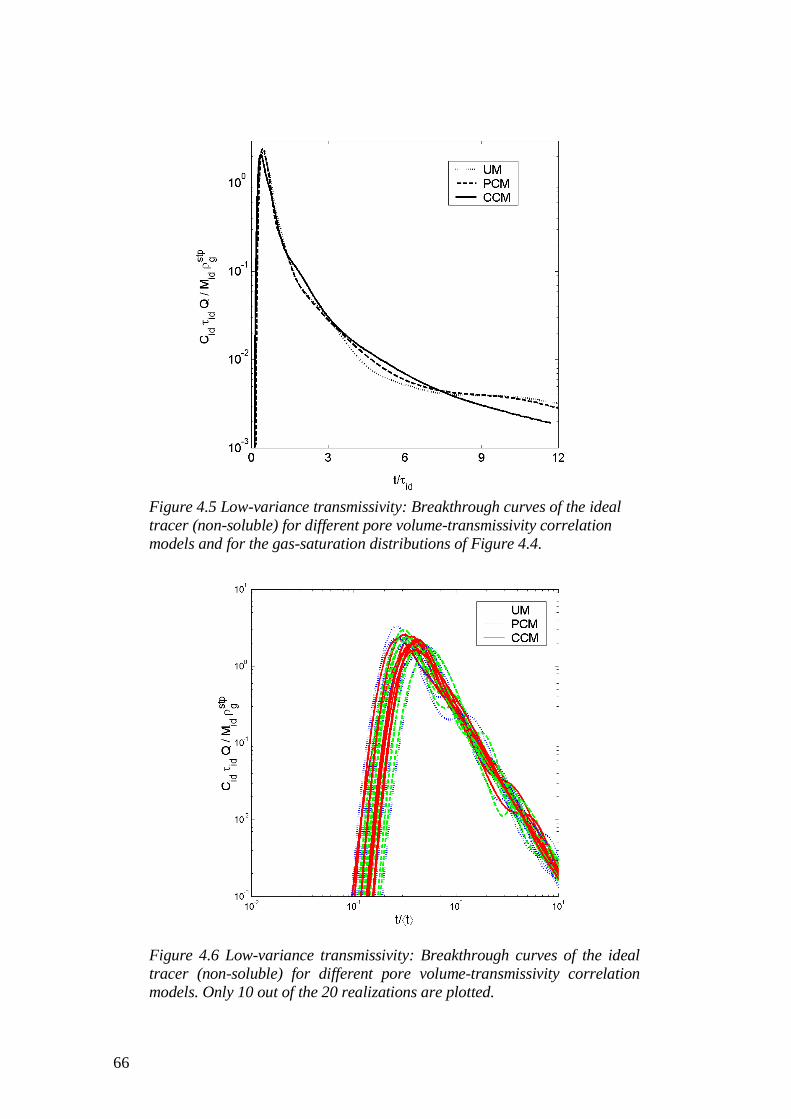
66

Figure 4.5 Low-variance transmissivity: Breakthrough curves of the idealtracer (non-soluble) for different pore volume-transmissivity correlationmodels and for the gas-saturation distributions of Figure 4.4.

Figure 4.6 Low-variance transmissivity: Breakthrough curves of the idealtracer (non-soluble) for different pore volume-transmissivity correlationmodels. Only 10 out of the 20 realizations are plotted.

67

4.4.1 Low-variance transmissivity fields

The first stage of the test consists of a partial desaturation of the fracture to reach quasisteady-state conditions. Air is injected at a constant rate Q [kg/s] in one borehole, whilethe other borehole is assumed to be open, which means that the pressure of both phasesis atmospheric (no capillary pressure), i.e. atmext

wextg ppp == . According to Lunati

(2000) we characterise the two-phase system by a macroscopic capillary number, whichrepresents the ratio of viscous to capillary forces, i.e.

∗∗∗∗

∗

==Tp

Qg

p

p

kp

LU

dstpg

winjg

atm

d

wCAρρµ , (4.10)

where the star-variables represent the typical value of the naturally related quantities.Here we set the typical Darcy velocity LbQU g

∗∗ ρ~ , which accounts for air

compressibility, and the typical density within the fracture was estimated by using idealgas law and assuming that the pressure is close to the entry pressure, i.e.

atminjg

stpgg ppρρ =∗ . This gives for all the simulations presented in this paper a capillary

number 100~CA , which fully characterize the air migration together with thedimensionless number for the pressure equation 100~CA2 ∗=Φ dg

injgw pp µµ once the

capillary model is assigned (see Appendix C for details).

When air injection starts, the fracture is fully saturated and the gas phase fills only theinjection borehole. The gas pressure in the borehole rises till it overcomes the entrypressure around the well, then air starts flowing into the formation displacing water,which is collected at the extraction borehole. Once the gas phase breaks through theextraction borehole, air starts to be recovered and the pressure at the injection boreholedrops considerably. After a while the gas saturation within the fracture can beconsidered steady state for our purposes (quasi steady-state), i.e. it varies slowly overthe typical residence time of the tracer. Figure 4.4 shows the quasi steady-statesaturation distribution for all three pore volume-transmissivity models obtained bynumerical simulations performed with TOUGH2 (Pruess, 1987). It is evident that evenfor low-variance transmissivity fields the choice of a conceptual model strongly affectstwo-phase flow via the capillary pressure. Indeed, according to equations (4.3) and(4.5), the space-dependent entry pressure in the UM produces a more heterogeneousgas-saturation distribution, because it depends directly on the transmissivity field: themost permeable regions have the highest gas content, therefore differences betweenmore and less permeable regions are amplified – compare equation (4.4). The gas flowmostly takes place in few channels characterized by above-average gas saturation andembedded in a low-saturation region. In contrast, the CCM has an entry pressure that isconstant in space, such that the saturation is determined by the pressure field, and thusonly indirectly by the transmissivity field, which yields a gas phase almost uniformlydistributed throughout the fracture. The PCM shows an intermediate behaviour with agas-phase pattern very similar to the UM, but a lower variability: sharp variations in thesaturation are smoothed by the correlation between pore volume and transmissivity.Note that despite of important differences in the gas-phase spatial distribution, the total

68

volumetric fraction of the system occupied by air is very similar in all models, i.e.around 20% of the total pore volume pV for all the realisations of the ensemble.

It is now clear that the identification of an appropriate conceptual model is an importantissue, because a wrong assumption on the correlation between pore volume-transmissivity prevents any model from adequately reproducing two-phase flow in thefracture. In practise, the main problem is that we can never observe the saturationdistribution and we have to deal with scarce information obtained by measurements atfew discrete locations – typically available only at the extraction and injection wells.The behaviour of the system has then to be inferred from these scarce data, whichseriously affects the possibility of success. In situ we normally control the injection rateQ, while pressure at injection well, gas and water outflow rate at the extraction boreholeare recorded as function of time. The former quantity can be accurately monitored, but itdoes not allow discriminating among he conceptual models, because the signals are verysimilar and almost indistinguishable. Gas outflow, in contrast, can be hardly measuredwith sufficient precision because of both technical limitations and strong fluctuationduring the desaturation processes (Fierz et al. 2000; Trick et al. 2000; Trick et al. 2001).This makes it difficult to have reliable data to perform an analysis of the water/gas ratioand also to determine the amount of gas in the fracture. The latter problem can be easilyovercome by performing a gas tracer test in the established gas-phase.

During the second stage of the gas tracer test, a known mass iM [kg] of the tracer i isinstantaneously injected at the recharging well (pulse injection) and the concentration

)(tCi is recorded at the extraction well for a time interval t∆ , which is the duration ofthe experiment. From these quantities the mass recovery curve can be computed as

iigi MttCQtMR d)()()( ∫= ρ . The tracer breakthrough curve )(tCi represents the

residence time distribution of the solute particle and the recovery curve )(tMRi is thecumulative probability function of the residence times, such that the tracer mean-arrivaltime can be calculated as

)(

d)()(

tMRM

ttCQt

ii

i

atmg

i ∆= ∫

ρτ . (4.11)

If dispersion is negligible, we can relate the mean-arrival time of the ideal tracer to theequivalent mass of gas in the fracture, i.e. idg QM τ= , or to a stp-equivalent gas volume

atmgid

stpg QV ρτ= . The water-soluble tracers experience a larger effective volume (or

gas mass) because of the retardation coefficient (4.7). From the arrival time distributionof the tracers it is then possible to compute a streamline-dependent retardation factor byidentifying a streamline via the mass recovery at the arrival time. Since the massrecovery is a monotonically increasing function, it can be inverted and we write

)(

)()(

MRt

MRtMRR

id

ii = . (4.12)

69

Figure 4.7 Low-variance transmissivity: mass recovery curve at theextraction well of tracers with a different water solubility for the gas-saturation distribution of Figure 4.4. From top to bottom: UM, PCM, CCM.

70

Writing equation (4.12), we assume that the arrival order of the streamlines is the samefor different. In other words, we assume that streamlines cannot overtake each other dueto the retardation factor experienced by soluble tracers. Since the retardation factor is amonotonically decreasing function of the gas saturation (figure 4.2), this assumption isjustified also in heterogeneous saturation fields as the UM or PCM, because thesaturation is highest in regions with the highest permeable regions. Inserting equation(4.12) into equation (4.7) we can compute a streamline effective saturation, which is aharmonic mean (weighted by the inverse of the velocity) of the gas saturation along thestreamline, i.e.

[ ][ ]

1

1

1

d)(

d)()()(

−

−

−

=∫

∫MR

MR g

gssu

ssusSMRS . (4.13)

Figure 4.8 Low-variance transmissivity: Effective gas saturation as afunction of mass recovery at the extraction well for different pore volume-transmissivity correlation models and realisations. Data from hydrogensulphide are used. Only 10 out of the 20 realizations are plotted.

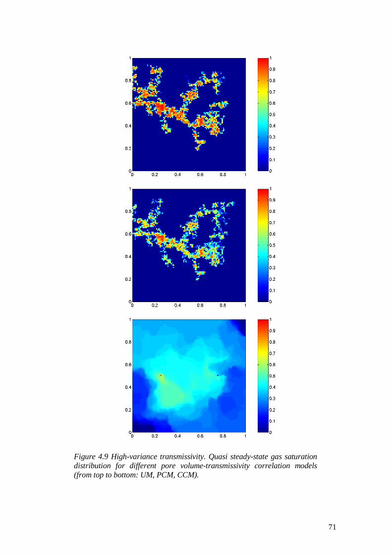
71

Figure 4.9 High-variance transmissivity. Quasi steady-state gas saturationdistribution for different pore volume-transmissivity correlation models(from top to bottom: UM, PCM, CCM).

72

Numerical simulations were performed with MODFLOW (McDonald and Harbaugh,1988) solving the pressure equation in 2

gp to account for gas compressibility, and with

MT3DMS (Zheng and Wang, 1998) simulating the transport of non-retarded andretarded tracers. The BCs of an ideal tracer injected into the three gas-saturation fieldsof figure 4.4 are shown in figure 4.5. The concentration is made dimensionless by thetotal mass of the tracer per stp-equivalent gas volume in the fracture, stp

pi VM , and the

time by the mean arrival time of the tracer, idτ . The normalized BCs corresponding tothe different models are very similar, both maximum concentrations and mean-arrivaltimes are very close in all three models despite of the different gas-saturationdistribution, thus velocity field. This is due to the inherent nature of breakthroughcurves that suffer from averaging at the extraction well where contributions fromdifferent streamlines are mixed. Only minor differences are noticeable, as for examplesome effects of heterogeneity of the velocity field, which are visible in the BC tail of theUM and PCM. This is confirmed by observation of the ensemble behaviour: the UMand the PCM are more likely to show a fluctuating-tail BC, whereas the CCM normallyproduces a smoother BC (figure 4.6). This is more a tendency than a discriminatingrule, because some realizations produce a fluctuating-tail BC also if the CCM isadopted.

Figure 4.10 High-variance transmissivity: Breakthrough curves of the idealtracer (non-soluble) for different pore volume-transmissivity correlationmodels and realizations.

Also considering soluble tracers, the differences among the conceptual models areminor. In figure 4.7 the mass recovery of all tracers is shown as a function of thedimensionless time, idt τ . Since a log-scale is employed for the dimensionless time, the

73

horizontal distance between two curves is proportional to the logarithm of theretardation factor. Thus, the picture shows that the order of magnitude of gas saturationis the same in all three models, as can be seen in figure 4.4. The streamline effectivesaturation computed according to equations (4.7) and (4.12) is plotted in figure 4.8 forall models and different realizations. The retardation of hydrogen sulphide is used. Thispicture clearly shows the partitioning-tracer properties of soluble tracers and the abilityof gas tracer tests to estimate the gas saturation in the fracture by comparing therecovery curves of a pair of water-soluble tracers. The CCM produces a curve that issmoother than the other two models. In particular the first part of the curve is almostflat, which means that the early streamlines experience a very similar effective gassaturation, such that differences in the saturation, if they exist, are averaged out alongthe streamlines. This is consistent with the fact that in the CCM the gas distribution isdominated by the pressure field and with the kind of saturation field on the bottom offigure 4.4. The other two models exhibit a larger variability from realization torealization. It is noticeable the different behaviour of the curves for the very earlystreamlines: a small amount of mass experiences a slightly higher saturation than theimmediately later streamlines. This is consistent with channelling and with a long-length correlation perpendicular to the flow: the first arrival takes place throughstreamlines travelling in a higher-saturated channel.

To summarize, we observe that even a small variance has remarkable effects on the gasdistribution within the fracture. The velocity field and the saturation field vary smoothlyall over the fracture in the CCM, whereas in the UM and PCM they vary withinchannels (streamline clusters) embedded in a low gas-saturation region. Neverthelessthe sensitivity to these effects of measurements at the extraction well is minor, becauseinformation is averaged by mixing over different streamlines, which makes the twocases hardly indistinguishable.

4.4.2 High-variance transmissivity fields

The numerical simulations presented above for low-variance transmissivity fields arerepeated using more heterogeneous fields, all flow-parameters except the log-transmissivity variance being unchanged. The effect of increasing the variance is toemphasize channelling in the UM and PCM. This is well-visible in the extreme caseshown at the top of figure 4.9, where the gas flow reduces to a single, highly saturatedchannel, producing a sort of shortcut between injection and extraction wells. In all therealisations of the high-variance ensemble gas flow takes place only in few discretechannels separated by fully water-saturated regions, if the UM is adopted. Strikingdifferences are noticeable compared to the CCM (bottom of figure 4.9), which stillproduces a continuously distributed gas phase. Also at high-variance the gas saturationin the CCM is determined by the pressure field and results in a more irregular patterndue to the more irregular pressure field. The PCM is once again in between, showing apattern similar to the UM, but characterized by a smaller variability of the saturation:extreme values are smoothed out by the correlation between pore volume andtransmissivity, which in turn decreases the correlation between entry pressure andtransmissivity. The dimensionless BCs of the ideal tracer for all realisations and modelsare shown in figure 4.10. The variability in the BC-tail increases for all models, whencompared to the low-variance ensemble (figure 4.6). The most noticeable difference is

74

that the CCM shows in general an earlier dimensionless first-arrival time and peak-arrival time than the other two models (see also table 4.2). Since the time is normalizedby the mean arrival time idτ , this suggests that the residence time distribution is moredispersed in the CCM. This is due to the fact that in the CCM the flow is fully two-dimensional, whereas in the other two models the residence-time dispersion is reducedbecause the streamlines are pulled together into channels. This smaller dispersion isconfirmed also by figure 4.11, which shows the mass recovery curves obtained fortracer tests performed in the gas-saturation fields of figure 4.9. The less steep recoveryof the CCM is a common characteristic of all realizations and confirms that the CCMproduces a more dispersed residence-time distribution.

Considering tracers with a different solubility allows identifying important differencesamong the models: in the CCM the retardation experienced by soluble tracers isconsiderably larger than in the other two models. In addition, the UM clearly shows thatdifferent tracers have mass recovery curves with different steepness, which means thatthe streamline effective retardation increases with time. The streamline effectivesaturation computed from hydrogen-sulphide retardation is plotted in figure 4.12 for allmodels and realizations. This picture definitely demonstrates the capability ofestimating the fracture saturation by gas tracer tests, since it clearly proves that in theUM and PCM flow takes place in regions with higher gas saturation than in the CCM asit is shown in figure 4.9. Most realizations produce a non-monotonic saturation curvewhen the UM or the PCM is adopted, which clearly proves the presence of well-separated channels. Indeed a channel represents a cluster of streamlines in which gassaturation exhibits a long stream-wise correlation and a short correlation in directionperpendicular to the flow. If the saturation curve is non-monotonic, at least two pathsexist with different lengths, which yield different arrival times. Maxima of the curverepresent contributions of different channels. Minima represent the contributions of theleast gas-saturated streamlines of a channel before the fastest, more gas-saturatedstreamlines of the next channel breakthrough at the extraction well producing a newmaximum. If the pressure field determines the gas-saturation distribution as in theCCM, the correlation in the direction perpendicular to the flow direction is large, suchthat streamlines with similar length have also similar gas saturation. That makes it veryunlikely, even in very heterogeneous fields, that a streamline exists with a breakthroughat the extraction borehole earlier than that of another streamline, which has higher gassaturation. For these reasons the saturation curve is monotonically decreasing.

Realization 6 exhibits an anomalous behaviour when compared to the averagebehaviour of the ensemble, namely much earlier first-arrival and peak-arrival times(figure 4.10). The streamline effective saturation curve (figure 4.12) indicates thepresence of two well-distinct regions with a very different saturation, which explains thefact that a large amount of tracer (around 60%) is travelling very fast to the extractionwell in a highly gas-saturated region ( 6.0=gS ). That is exactly what happens in the

fracture as it can be observed in figure 4.13, which shows the gas-saturation distributionin realization 6 when the CCM is adopted. This definitely proves the ability of inferringthe gas saturation distribution in the fracture by partitioning gas tracer tests.

75

Figure 4.11 High-variance transmissivity: mass recovery curve at theextraction well of tracers with a different water solubility for the gas-saturation distribution of Figure 4.9. From top to bottom: UM, PCM, CCM.

76

Figure 4.12 High-variance transmissivity: Effective gas saturation as afunction of mass recovery at the extraction well for different pore volume-transmissivity correlation models and realisations. Data from hydrogensulphide are used.

Figure 4.13. High-variance transmissivity: Quasi steady-state gasdistribution for realization 6 when the CCM is adopted.

77

Finally, we compare the streamline effective saturation computed from the retardationof differently soluble tracers, i.e. xenon and hydrogen sulphide. These curves are shownin figure 4.14 as a function of the mass recovery for realization 6. Even in this particularrealisation the two curves are indistinguishable in the CCM, whereas in the other twomodels the differences between the saturation computed from xenon or hydrogen-sulphide retardation are sensitive. This has to do either with interactions amongstreamlines (diffusion) or with changes in the streamline arrival order produced by thedifferent retardation coefficients. Both phenomena are neglected in our analysis yieldingthe streamline effective retardation and gas saturation, they can however be important ina gas saturation field characterized by a long stream-wise correlation and a shortcorrelation perpendicular to the flow, as in the UM and PCM. In such fields, it ispossible that a mass of tracer travelling on a streamline can move by dispersion toanother streamline with a considerably different gas saturation or that a streamline is“overtaken” by a close streamline with a higher gas saturation when a soluble tracer isconsidered. Both phenomena are very unlikely if the CCM is adopted, because of thelong correlation in the direction perpendicular to the flow.

Figure 4.14 High-variance transmissivity: Effective gas saturation as afunction of mass recovery at the extraction well for realisation 6 and thethree conceptual models. Both data from xenon and hydrogen sulphide areused.

78

ModelFirst arr. time

( 30 10−=CC )[-] Peak arrival time [-] 25%-recovery time [-]

UM0.154 ± 0.020

(S.D.=0.056)

0.418 ± 0.034

(S.D.=0.097)

0.45 ± 0.03

(S.D.=0.08)

PCM0.163 ± 0.021

(S.D.=0.060)

0.492 ± 0.060

(S.D.=0.170)

0.49 ± 0.05

(S.D.=0.14)

CCM0.055 ± 0.013

(S.D.=0.037)

0.281 ± 0.056

(S.D.=0.158)

0.32 ± 0.05

(S.D.=0.14)

Table 4.2 High-variance transmissivity: Mean values averaged over 7realizations of first arrival, peak arrival and 25%recovery dimensionlesstime ( idt τ ) and their standard deviation for different pore volume-transmissivity correlation models. In bracket the standard deviation of theensemble.

4.5 Conclusions

The conceptual model adopted for the pore volume-transmissivity correlation has astrong effect on the saturation of the fracture via the entry pressure, which can be relatedto the transmissivity in a different way according to the different conceptual model.Even in low-variance transmissivity fields the UM shows a very heterogeneous gasdistribution: gas flow takes mainly place through preferential paths characterized byabove-average gas saturation and embedded in a low-saturation region. Due toLeverett’s model and relative permeability, differences between high and low-transmissivity regions are amplified, when compared to flow in a fully water-saturatedfracture. A correlation between pore volume and transmissivity tends to smooth thedistribution of the gas-phase, because it reduces the correlation between transmissivityand entry pressure. In particular, a complete correlation between pore volume andtransmissivity (CCM) requires that permeability is constant in space, which correspondsto a rough-walled fracture filled with a homogeneous fault gouge. This implies that theentry pressure is constant in space and yields a smoother gas-saturation field, since it isdetermined only by the pressure field, thus only indirectly by the transmissivity. ThePCM, as for example an empty-fracture model, produces a gas-phase pattern verysimilar to the UM, but with slightly reduced variations of the saturation. If high-variance transmissivity fields are considered, differences become striking: in the UMand in the PCM the streamlines collapse into few channels characterized by very highgas saturation and separated by water saturated regions inaccessible to gas flow. In theextreme case, the flow between producing and recharging wells takes place in a singlechannel (shortcut). In contrast, the CCM yields a gas flow that still takes place in a morewidely spread region where the gas saturation is considerably smaller than in thechannels produced by the other two models.

79

These differences in the saturation can be very well observed by means of a gas tracertest in which at least two tracers with different water-solubility are employed. Wedemonstrate that this technique provides an excellent tool to estimate the fracturesaturation by computing a streamline-averaged saturation. The tracers dissolve into thewater phase according to their solubility, which is known, and to the amount of wateravailable. By comparing the residence-time distribution of two tracers we can computea streamline retardation factor, from which we can extrapolate a streamline effectivesaturation. This technique also provides additional information to that obtained by aclassical tracer tests and helps to discriminate among the conceptual models: a non-monotonically decreasing curve of the streamline effective saturation as a function ofmass recovery clearly proves the presence of well-separated channels within thefracture, which is normally observed in the UM or PCM. This behaviour, which isproduced by a long stream-wise correlation of the gas saturation, is not expected in theCCM. In extreme cases in which only one channel is present (shortcut) the UM andPCM also produce a monotonic streamline saturation curve, but differences from theCCM can be observed as the arrival-time distribution is less dispersed. This is due to thefact that flow in a channel is similar to mono-dimensional flow, whereas the CCMalways produces a completely two-dimensional flow, because of the smoother and morewidely spread saturation distribution. If more than two soluble tracers are available, acomparison of the effective saturation computed from the retardation of different tracersis also very helpful to discriminate among the models. Indeed, in the smoothlydistributed gas phase of the CCM all tracers yield the same saturation. In contrast, thesaturations computed from different tracers show sensitive differences in the UM andPCM. The correlation of the saturation field, long in the flow-direction and short in theperpendicular direction, can change the streamline-arrival order with regard to thesolubility of the tracers, which experience different streamline retardations. Suchcorrelation might also make small dispersive effects important, because they can movethe tracer from one streamline to another with a considerably different saturation. Bothphenomena, which are neglected in our analysis yielding the streamline effectiveretardation and gas saturation, can produce slightly different curves if data fromdifferent tracers are used. However one should acknowledge that in practise manyfactors might complicate the calculation of an accurate effective saturation, such asrelatively large dispersion, kinetics of the dissolution (non-instantaneous equilibrium) oradditional chemical reactions.

To conclude, discrimination among conceptual models by means of measurement at theextraction well are a difficult issue, due to the nature of these measurements themselves,which suffer from averaging over different streamlines. Nevertheless, tests that use gas-tracers with different water solubility, provide important information about saturation inthe fracture and are very useful in discriminating between the UM and the CCM in themost important case of high-variance transmissivity fields. The UM and PCM remainindistinguishable on the basis of data from gas tracer tests, essentially due to the minordifferences of the gas-saturation field, which makes their behaviour very similar.

80

4.6 Appendix B

A tracer phase is transported in the gas-phase according to

( ) ( ) ( )[ ] gwiiigggiggigg qqXnSXnSXnS

t→=−⋅−⋅+

∂∂ ρρρ ∇∇∇∇∇∇∇∇∇∇∇∇ Du , (B.1)

where the term on the right hand side describes the mass transfer between gas and waterphase, and it is given by

( )wiww

gwi XnS

tq ρ

∂∂−=→ , (B.2)

where wiX is the mass fraction of the component i in the water phase [kg/kg]. By

assuming instantaneous equilibrium, the molar fractions in the two phases are related byHenry’s law, i.e.

igw

i xH

px = . (B.3)

where wix , resp. ix , is the molar fraction in the water, resp. gas, phase [mol/mol] and H

the Henry’s constant [kg/ms2]. That yields for the mass fractions

ig

w

gi

g

w

iwi

w

iwi X

H

p

W

Wx

H

p

W

Wx

W

WX === , (B.4)

where βW is the molar weight of β [kg/mol]. By inserting (B.4) into (B.2) one easily

obtains

−∂∂−=

∂∂−=→

iw

gw

g

g

g

gggi

g

w

gww

gwi X

HW

Wp

S

SnS

tX

H

p

W

WnS

tq

11ρ

ρρρ . (B.5)

By inserting (B.5) into (B.1) and using the ideal gas law, i.e.

g

AB

g

g

W

NKp θρ

= (B.6)

where θ is the temperature [K], BK is Boltzmann’s constant [kg m2/s2 K] and NA theAvogadro constant [1/mol]. Finally, we define a solubility factor

w

wABi WH

NK ρθγ = (B.7)

81

and we obtain equation (4.6) with a retardation coefficient iR given by equation (4.7).

4.7 Appendix C

The system of equations that describes two-phase flow can be reformulated to obtain afirst equation for the gas pressure, gp , and a second equation for the gas saturation, gS ,

which together with equations(4.3), (4.4) and the constitutive relationships determinethe flow (see e.g. Helmig, 1997). In particular, one obtains a non-linear transportequation for the gas saturation, which is physically rescaled by Lunati (2000), whointroduces the macroscopic capillary number (4.10). With the gas-pressure equation(4.2) using the Darcy velocity given by (4.1) we naturally associate a dimensionlessnumber

d

pp

gbU

T

d

pp

U

kextg

injg

wg

w

extg

injg

g

−=

−=Φ ∗

∗

∗

∗

ρµµ

µ1

(C.1)

As typical Darcy velocity we take

Lb

Q

p

p

Lb

QU

stpg

injg

atm

g ρρ== ∗

∗ , (C.2)

where we estimate the pressure within the fracture by the pressure at the injection well.By introducing equation (C.2) into equation (C.1) we obtain

( )Qpg

Tp

d

Latm

injg

wg

stpgw

2 ∗

=Φρµρµ

(C.3)

where we use extg

injg pp >> . The first coefficient is a geometric factor (ratio of the

domain to the dipole size), the second a fluid factor, which depends on the characteristicproperties of the two fluids.

Acknowledgements

We gratefully acknowledge financial support of NAGRA, the National Cooperative forthe Disposal of Radioactive Waste, Switzerland.

82

83

Chapter 5

Two-phase Flow Visualization in a Single-fracture byNeutron Radiography

I. Lunati, P. Vontobel, W. Kinzelbach, and E. Lehmann

5.0 Abstract

Due to their weak interaction with the matter, thermal neutrons are highly penetratingand can used as non-destructive probe for complex structures. As water has a highmacroscopic cross section, neutron radiography is suitable to investigate moisturecontent of rock samples. We use neutron tomography to visualize imbibition anddrainage in a core containing a fault-gouge filled fracture. During capillary imbibitionthe wet front rises rapidly. After a few minutes it assumes an almost steady-state profileand then a slow increase of moisture content in the already wet regions is observed. Wesuggest that water first fills a well-connected porosity then it is slowly sucked into apoorly connected porosity. By comparison of tomographic images of the sample beforeand after imbibition we observe an uneven water distribution. The drainage experimentis performed by injecting air into the previously saturated sample. The waterdistribution in the fracture is observed before and after drainage. This shows that the airphase is very irregularly distributed, supporting that air flows through preferential paths.

Keywords: Neutron tomography; shear zone; fault gouge; capillary imbibition;drainage.

84

85

5.1 Introduction

Heterogeneities of fracture properties may yield unevenly distributed multiphase flowand transport. The behaviour of the system strongly depends on the pore-volumedistribution and the nature of the heterogeneities. Lunati et al. (2003, also chapter 3)demonstrate that solute transport strongly differs in an empty fracture or in a fracturefilled with a homogeneous fault-gouge. If two-phase flow is considered, the differencesare even more striking due to the role played by the entry pressure (Lunati andKinzelbach, 2003, also chapter 4). In case of a complicated structure such as a shearzone in crystalline rocks, it is desirable to directly observe flow and transportphenomena and assess whether the flow takes place in few preferential paths or isevenly distributed all over the fracture.

Non-destructive investigation of two-phase flow in a granite core was attempted byChen and Kinzelbach (2002) by nuclear magnetic resonance (NMR). This techniqueessentially sees the signal of hydrogen nuclei, which align their magnetic moment to theapplied magnetic field. From the transverse relaxation time of the nuclei information onthe size of the water-filled pores can be obtained. However, due to the paramagneticproperties of granite, only low-intensity magnetic fields can be applied, which preventsthe measurements from having a good spatial resolution. Only the overall pore-sizedistribution can be measured. A technique, which allows better spatial distribution, isneutron radiography. This technology was used in the past to investigate the moisturedistribution in different materials (Lehman et al., 1999; Lehmann and Vontobel, 2000;Pleinert et al., 1998; Pleinert and Degueldre, 1995; Degueldre et al., 1996). We useneutron radiography to investigate two-phase flow in a core containing a fault-gougefilled fracture. We study both capillary imbibition in the dry sample and drainage by airinjection in the saturated sample.

Figure 5.1. Interaction of neutrons with matter and exponential attenuationlaw for a narrow beam (http://neutra.web.psi.ch/)

86

5.2 Neutron radiography: Theoretical background and technology

Neutrons are, with protons, one of the two components of the atomic nucleus. They areuncharged particles so that in contrast to x-rays (photons) they do not interact with theelectron shell of atoms but only with the much smaller nuclei. Therefore neutronsinteract essentially with protons and are quite sensitive to light atoms, most of all tohydrogen. Due to this weak interaction with matter, they are highly penetrating and canused as non-destructive probes for complex structures.

Table 5.1 Structural materials for neutron transmission measurements;composition and macroscopic cross-section for interaction with thermalneutrons (25meV); data for water added for comparison. (After Lehmannand Vontobel, 2000)

The transmission behaviour of a neutron beam can be described by the simpleexponential attenuation law (figure 5.1)

)exp(0 dII Σ−= , (5.1)

where I is the intensity of the transmitted beam [n/m2s], I0 the intensity of the incidentbeam [n/m2s], d the thickness of the sample [m], and Σ the macroscopic cross section[m-1]. Deviations from equation (5.1) have to be expected and taken into account forthick samples or strongly interacting material, due to multiple scattering or to changesin the energy spectrum. We remark the differences of neutron radiography whencompared with classical x-ray radiography. Even though x-ray attenuation is alsodescribed by an exponential law, the linear attenuation coefficient µ [m-1] (analogous tothe macroscopic cross section Σ) is different and increases rapidly with the atomicnumber Z, i.e. µ~Z3.8, such that they are more effectively attenuated by heavy materialslike metals, whereas Σ is higher for some light materials with a high number of single

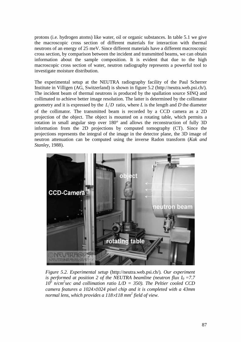
87

protons (i.e. hydrogen atoms) like water, oil or organic substances. In table 5.1 we givethe macroscopic cross section of different materials for interaction with thermalneutrons of an energy of 25 meV. Since different materials have a different macroscopiccross section, by comparison between the incident and transmitted beams, we can obtaininformation about the sample composition. It is evident that due to the highmacroscopic cross section of water, neutron radiography represents a powerful tool toinvestigate moisture distribution.

The experimental setup at the NEUTRA radiography facility of the Paul ScherrerInstitute in Villigen (AG, Switzerland) is shown in figure 5.2 (http://neutra.web.psi.ch/).The incident beam of thermal neutrons is produced by the spallation source SINQ andcollimated to achieve better image resolution. The latter is determined by the collimatorgeometry and it is expressed by the DL ratio, where L is the length and D the diameterof the collimator. The transmitted beam is recorded by a CCD camera as a 2Dprojection of the object. The object is mounted on a rotating table, which permits arotation in small angular step over 180° and allows the reconstruction of fully 3Dinformation from the 2D projections by computed tomography (CT). Since theprojections represents the integral of the image in the detector plane, the 3D image ofneutron attenuation can be computed using the inverse Radon transform (Kak andStanley, 1988).

Figure 5.2. Experimental setup (http://neutra.web.psi.ch/). Our experimentis performed at position 2 of the NEUTRA beamline (neutron flux I0 =7.7106 n/cm2sec and collimation ratio L/D = 350). The Peltier cooled CCDcamera features a 1024×1024 pixel chip and it is completed with a 43mmnormal lens, which provides a 118×118 mm2 field of view.

88

Our experiment is performed at position 2 of the NEUTRA beamline (neutron fluxscmn107.7 26

0 =I and collimation ratio 350=DL ). A Peltier cooled CCD camera

featuring a 1024×1024 pixel chip is used completed with a 43mm normal lens, whichprovides a 118×118 mm2 field of view. The spatial resolution is set by the pixel size115×115 µm2. The sample fixed on the rotary table in front of a 0.2 mm thickscintillator screen based on 6LiF:ZnS:Cu, is rotated from 0o to 180o in 0.6o angularsteps. The resulting projection images are corrected for flat-field inhomogeneity andCCD background noise, as well as for the neutron flux fluctuation during theexperiment.

5.3 The Fracture Sample

5.3.1 Core drilling

The core is drilled in the Grimsel Granodiorite at the GAM experimental site (AUtunnel, location 144 m, core GAM02-001) in the Grimsel Underground Laboratory (BE,Switzerland). The core-drilling technique was developed during several campaigns ofGAM, in which different methods were tested to identify the least disturbing one(Marschall, 1998). Eight bore holes with diameter 32 mm are predrilled to a depth ofabout 400 mm; the arrangement of the eight boreholes is circular (uniformly distributedon a circle with diameter of about 125 mm; see figure 5.3). The bore-holes are filled byepoxy resin and after hardening, an annulus is drilled to a depth of about 400 mm. Freshwater is used as drilling fluid, since it was demonstrated during several drillingcampaigns that dry drilling presents a high risk of damaging the core and takes muchlonger. Nevertheless little water is used in order not to flush the fault gouge from thefracture. Then, the annulus is at its turn filled by epoxy resin and, after hardening, over-cored to a depth of about 500 mm. The sample is broken out at the depth of the over-coring annulus.

5.3.2 Preliminary non-invasive investigation by X-ray CT scan

The two faces are made regular by sawing, which reduces the high of the core to 290mm. At the upper face four fractures are visible (figure 5.3), which contain a non-cohesive fault gouge material. At the lower face fractures III and IV merge into acomplex structure forming a highly fractured area with a thickness of about 22 mm; theother two fractures remain well separated. As we want to focus on the effects of small-scale heterogeneity, it is preferable to perform the experiments in a single fracture. Thisallows distinguishing the effects of variable thickness and fault-gouge properties fromlarger-scale heterogeneity such as fracture intersections and geometry of the fracturenetwork, for which our sample cannot be considered representative.

To select the optimum fracture to perform the experiments, we first investigated theinternal structure of the sample by X-ray CT. The core is scanned under dry conditionsby CT using a 423 kV tube voltage and 2.1 mA tube current. The horizontal slicethickness is 4 mm and the maximum imaging matrix is 500×500 pixels (0.36×0.36 mm2

pixel size, 180×180 mm2 image size). Eleven uniformly spaced sectional images were

89

obtained from a depth of 25 mm to a depth of 275 mm (step 25 mm). On the basis ofdata from CT, we select fracture II between a depth of 20 mm and 180 mm.

5.3.3 Core processing

At this stage the sample is a 293 mm high cylinder with a diameter 173 mm andcontains an epoxy matrix embedding the fractures (figure 5.3). Since epoxy resin, aswell as any other plastic material, has a large macroscopic cross section for thermalneutrons (Σ = 130 cm-1 at 26 meV), the sample has to be sub-cored and a new materialhas to be used as matrix to keep the fracture tight. Aluminium represents the best choicebecause it is not activated by the neutron beam and has a very low macroscopic crosssection, Σ = 0.10 cm-1. The relatively high melting temperature (660° C) could damagethe sample and makes it difficult, to work with melted aluminium. Thus, we decide tomould an aluminium tube to the sub-core.

Figure 5.3 Upper face of the core before processing. Four fractures arevisible; the fracture selected for the experiment is designed by II. The dash-lined circle approximately represents the sub-coring position.

Two boreholes (diameter 32 mm, minimal distance 57 mm) are drilled to a depth of 220mm at the side of fracture II and filled with a mortar. The purpose is multiple: sealingthe fracture (at least partially) to prevent a significant secondary flow between Al-tubeand granite; keeping together the two half-cylinders that form the fracture; protectingthe fracture against flushing of the fault gouge during sub-coring, which requires a largeamount of cooling fluid to obtain a precise bore-hole. The ideal material to fill up the

90

bore-holes has to be an optimal compromise among several requirements: smallmacroscopic cross section to be transparent to the neutron beam; wettability close togranite to avoid preferential paths of air flow at the boundaries; small porosity to avoidlarge amounts of imbibed water that strongly increases the beam attenuation; non-wetting properties in the liquid state to prevent the mortar from being imbibed bycapillary forces when casting, which may alter fracture properties; good mechanicalproperties to resist to the sub-coring stress. After considering different materials andtesting different mortars, a compromise is found by mixing 700 g quick-setting cement(CEM I AL), 1250 g sand with diameter 0÷4 mm, 180 g water and 10.3 gsuperplasticiser Glenium© 51 based on modified carboxylic ether. The macroscopiccross section of this mortar is measured as Σ = 0.25 cm-1, which is close to granite (seeTable5.1). The water wettability is assumed close to granite by visual inspection of thewetting angle formed by a water drop. The non-wetting property of the liquid mortar isconfirmed by the meniscus during the casting. After pouring the mortar into theboreholes, the sample is agitated for about 10 minutes to remove macroscopic airbubbles and prevent the formation of macro-pores. The core is stored for a week at20°C and 75% humidity to let the mortar harden and develop the mechanical properties.

Figure 5.4. Bottom view of the sub-cored sample. Two vertical mortarcolumns close fracture II, which is selected for the experiment. The otherfractures (I,III,IV) will be sealed with silicon to avoid secondary flow. Analuminium tube is moulded on the sub-cored sample to keep it tight

The sub-coring annulus is drilled to a depth of 175 mm by a drill with inner/outerdiameter 80 mm/87 mm. Care is taken to obtain a smooth and regular annulus bydrilling slowly and with abundant fresh water as drilling fluid. After drying the core for24 hours at 20°C and 45% humidity, a 160 mm high Al-tube (inner/outer diameter 79.5mm/83.0 mm) is pressed on the sub-core to a depth of 170 mm. The sample is cut

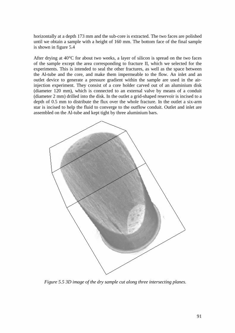
91

horizontally at a depth 173 mm and the sub-core is extracted. The two faces are polisheduntil we obtain a sample with a height of 160 mm. The bottom face of the final sampleis shown in figure 5.4

After drying at 40°C for about two weeks, a layer of silicon is spread on the two facesof the sample except the area corresponding to fracture II, which we selected for theexperiments. This is intended to seal the other fractures, as well as the space betweenthe Al-tube and the core, and make them impermeable to the flow. An inlet and anoutlet device to generate a pressure gradient within the sample are used in the air-injection experiment. They consist of a core holder carved out of an aluminium disk(diameter 120 mm), which is connected to an external valve by means of a conduit(diameter 2 mm) drilled into the disk. In the outlet a grid-shaped reservoir is incised to adepth of 0.5 mm to distribute the flux over the whole fracture. In the outlet a six-armstar is incised to help the fluid to converge to the outflow conduit. Outlet and inlet areassembled on the Al-tube and kept tight by three aluminium bars.

Figure 5.5 3D image of the dry sample cut along three intersecting planes.

92

5.4 Experimental procedure

5.4.1 Capillary imbibition

We perform a first experiment to visualize the capillary rise of water in the dry sample.No pressure gradient is applied (the inlet and outlet devices are not assembled) andcapillarity is the only driving force. By comparing the transmission of neutrons throughthe sample before and after imbibition, we obtain information on water distribution. It isimportant that the position of the sample remains unchanged during the all experiment,such that the same pixels can be compared in the image processing. The sample isplaced in a glass container, which will be successively filled with water, and a 3D imageis acquired by neutron tomography. Due to the thickness of the core, a relatively longexposition time (around 40 sec) is needed in order to guarantee an adequate intensity ofthe transmitted beam and a satisfactory image resolution. Since the sample size is largerthan the field of view of the CCD camera, the overall tomography is obtainedcombining an upper-part tomography with a lower-part tomography. A 3D view of thedry sample cut along three intersecting planes is shown in figure 5.5.

Figure 5.6. Top-left corner: Dry-sample radiography, projection in thedirection perpendicular to the flow. Top center to bottom-right corner:ratios of the radiography at different times after capillary imbibition startedto the dry sample radiography (top-left corner). These ratios show the watercontent (black) in the core at times 32sec, 9min 53sec, 32min 39sec, 1h5min 54sec and 2h 5min 12 sec after the glass container is filled with water.

93

Figure 5.7: Two sections from the dry core (left) and from the core aftercapillary imbibition (right): Horizontal section (top); Vertical sectionparallel to the fracture plane (bottom). From left to right fractures I, II, IIIand IV (in contact with the Al-tube).

94

Figure 5.8: Two sections from the saturated core (left) and from the coreafter air injection (right): Horizontal section (top); Vertical section parallelto the fracture plane (bottom). From left to right fractures I, II, III and IV(in contact with the Al-tube).

95

Figure 5.9: Ratio imbibed to dry (left) and saturated to drained sample(right). A section parallel to the fracture plane is selected from a volumethat contains fracture II. Black represents pixels with higher water content.

After acquisition of fully three-dimensional information by tomographic reconstruction,the glass container is filled with water and capillary suction starts. Water rises rapidly,such that acquisition of 3D information is impossible because of the long time requiredfor a tomography. Thus, we observe the wet-front displacement by radiographies in thedirection perpendicular to the fracture. This restriction to a 2D projection of the coreallows a satisfactory temporal resolution with acquisition of an image every 30 sec(exposition time 10 sec). After 10 min an image every 1 min is acquired (expositiontime 30 sec). Each image is normalized by the radiography of the dry sample (top-leftcorner of figure 5.6), such that differences from the dry state are highlighted and waterdistribution results. The wet front at five time steps is shown in figure 5.6. Notice thatthe water content is integrated over the fracture thickness, since these are 2Dprojections. The front rises rapidly and after a few minutes the water appears irregularlydistributed. After that, an increase of moisture content in the already wet regions isobserved. We suggest that this reflects non-negligible conductivity effects duringunsteady imbibition: even if the height of the capillary rise is completely determined bycapillarity, imbibition might be slower if conductivity is low. A faster capillary

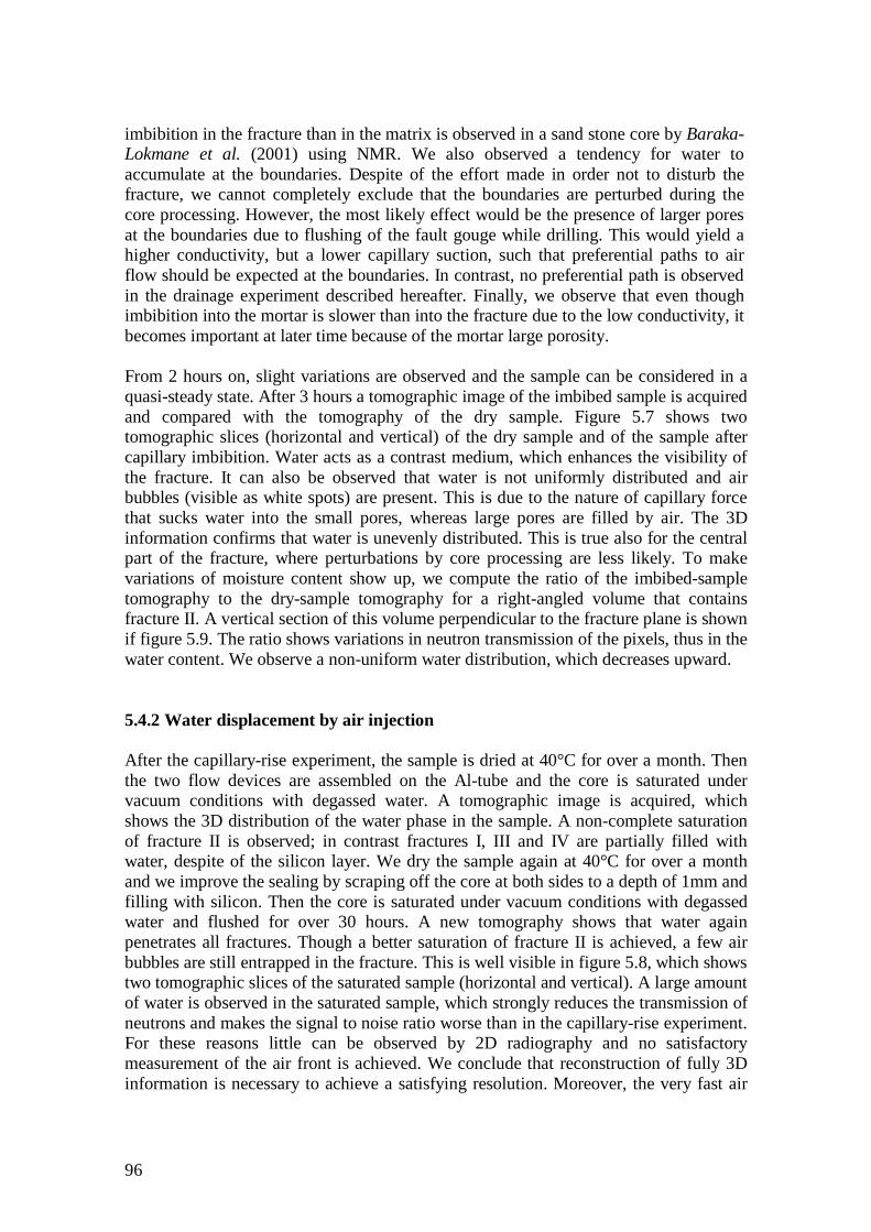
96

imbibition in the fracture than in the matrix is observed in a sand stone core by Baraka-Lokmane et al. (2001) using NMR. We also observed a tendency for water toaccumulate at the boundaries. Despite of the effort made in order not to disturb thefracture, we cannot completely exclude that the boundaries are perturbed during thecore processing. However, the most likely effect would be the presence of larger poresat the boundaries due to flushing of the fault gouge while drilling. This would yield ahigher conductivity, but a lower capillary suction, such that preferential paths to airflow should be expected at the boundaries. In contrast, no preferential path is observedin the drainage experiment described hereafter. Finally, we observe that even thoughimbibition into the mortar is slower than into the fracture due to the low conductivity, itbecomes important at later time because of the mortar large porosity.

From 2 hours on, slight variations are observed and the sample can be considered in aquasi-steady state. After 3 hours a tomographic image of the imbibed sample is acquiredand compared with the tomography of the dry sample. Figure 5.7 shows twotomographic slices (horizontal and vertical) of the dry sample and of the sample aftercapillary imbibition. Water acts as a contrast medium, which enhances the visibility ofthe fracture. It can also be observed that water is not uniformly distributed and airbubbles (visible as white spots) are present. This is due to the nature of capillary forcethat sucks water into the small pores, whereas large pores are filled by air. The 3Dinformation confirms that water is unevenly distributed. This is true also for the centralpart of the fracture, where perturbations by core processing are less likely. To makevariations of moisture content show up, we compute the ratio of the imbibed-sampletomography to the dry-sample tomography for a right-angled volume that containsfracture II. A vertical section of this volume perpendicular to the fracture plane is shownif figure 5.9. The ratio shows variations in neutron transmission of the pixels, thus in thewater content. We observe a non-uniform water distribution, which decreases upward.

5.4.2 Water displacement by air injection

After the capillary-rise experiment, the sample is dried at 40°C for over a month. Thenthe two flow devices are assembled on the Al-tube and the core is saturated undervacuum conditions with degassed water. A tomographic image is acquired, whichshows the 3D distribution of the water phase in the sample. A non-complete saturationof fracture II is observed; in contrast fractures I, III and IV are partially filled withwater, despite of the silicon layer. We dry the sample again at 40°C for over a monthand we improve the sealing by scraping off the core at both sides to a depth of 1mm andfilling with silicon. Then the core is saturated under vacuum conditions with degassedwater and flushed for over 30 hours. A new tomography shows that water againpenetrates all fractures. Though a better saturation of fracture II is achieved, a few airbubbles are still entrapped in the fracture. This is well visible in figure 5.8, which showstwo tomographic slices of the saturated sample (horizontal and vertical). A large amountof water is observed in the saturated sample, which strongly reduces the transmission ofneutrons and makes the signal to noise ratio worse than in the capillary-rise experiment.For these reasons little can be observed by 2D radiography and no satisfactorymeasurement of the air front is achieved. We conclude that reconstruction of fully 3Dinformation is necessary to achieve a satisfying resolution. Moreover, the very fast air

97

breakthrough (few tens of seconds) makes it difficult to follow the air front with thetemporal resolution that is available for this sample.

Figure 5.10. Ratio of the saturated-sample tomography to the drained-sample tomography for a selected volume. Black corresponds to higherwater content in the saturated sample than in the drained sample, thus toregions drained by air injection. Fracture II is well visible and lays in avertical plane in the middle of the volume.

The core is drained by injecting air at 1.5 bar pressure for 1 hour, then the valves of theflow devices are closed and a tomographic image is acquired. Figure 5.8 compares twotomographic slices of the saturated sample and of the sample after drainage. The effectsof drainage are well visible in fracture II, which becomes less visible. By inspection ofthe entire 3D image no preferential path to air flow is observed at the boundaries. Thissuggests that the fracture boundaries were not disturbed by core processing, whichwould produce higher and better connected pores by flushing the fault gouge. The waterdistribution in fractures I, III and IV shows only minor variations after drainage. As forthe data from the capillary-rise experiment, we select a right-angled volume containingfracture II and we compute the ratio of the saturated-sample tomography to the drained-sample tomography. A representation of this 3D volume is shown in figure 5.10.Fracture II is well visible and lies in a vertical plane in the middle of the volume. Thedarker regions correspond to higher water content in the saturated sample than in thedrained sample, thus they conversely represent the region drained by air injection. Thisis evidence that the air phase is unevenly distributed after drainage and testifies that airflows through preferential paths. In figure 5.9 a section of this volume perpendicular tothe fracture plane is compared with the result of the capillary-rise experiment.

98

5.5 Conclusions

Neutron radiography offers a good tool for non-destructive investigation of granitesamples. Due to the weak interaction with the core and the high macroscopic crosssection of water, neutron radiography provides a good instrument for visualization ofconductive paths: the water enhances the visibility of the porosity by strong attenuationof the neutron beam. This allows highlighting the part of porosity, which takes part in aparticular process.

A capillary imbibition experiment in a fault-gouge filled fracture shows an unevendistribution of water. The water front rises rapidly and after a few minutes it assumes analmost steady-state profile. After that, a slow increase of moisture content in the alreadywet region is observed. We suggest that water rapidly fills a well-connected porosityand then it is sucked slowly into a poor-connected porosity. Since only 2D projectionsof the dynamic process are available because of temporal-resolution constraints, it is noteasy to understand whether the poor connected porosity consists exclusively of fault-gouge material or includes the granite matrix. Nevertheless, the much smallerconnectivity and porosity (1.1% after Chen and Kinzelbach, 2002) suggest that theamount of water imbibed into the matrix is negligible. This double porosity model isconsistent with shrinking of the fault-gouge when drying, which has been observed(Chen and Kinzelbach, 2002). We suggest that water first imbibes the channel opened inthe dry sample by shrinking of the fault-gouge (well-connected porosity), than the fault-gouge itself, which represents the poor-connected porosity.

When the drainage experiment is performed by injecting air, the large amount of waterin the saturated core and the rapid air breakthrough prevent us from observing thedisplacement of the air front. Despite of the effort to saturate only one of the fourfractures in the core, water penetrates all of them, which yields a strong attenuation ofthe neutron beams such that fully 3D information is needed to obtain the necessaryresolution and observe variations of the moisture content. After drainage the air phase inthe fracture is very irregularly distributed, which testify that air flows throughpreferential paths. This is consistent with the quick air breakthrough, which implies asmall air volume in the fracture.

Acknowledgements

We are grateful to Thomy Keller for his technical support in core processing and forconstructing the inlet and outlet devices. We thank Paul Marschall, WolfgangKickmeier, and Hanspeter Weber for organizing the coring at the Grimsel Test Site;Giovanni Martinola, for his contribution in selecting and preparing the mortar; ThomasJaggi, for helping in the core processing. This project was supported by NAGRA(National Cooperative for the Disposal of Radioactive Waste) in the framework ofGAM (Gas and migration in shear zone).

99

Chapter 6

Synthesis and conclusions

When modelling a fracture we have to make several hypotheses on its internal structureand assume relationships among different properties of the medium in order to be ableto build a physically based model of the system. In other words we have to assume aconceptual model, which guides us in making assumptions over the processes that takeplace in the system. We demonstrate that conceptual model assumed to interpretmultiphase transport in single fractures strongly affects the predictive capability of themodel itself. We show by experimental observations and numerical simulations that thechoice of an adequate model is fundamental to reproduce the behaviour of the system.Different conceptual models show not only quantitative, but also qualitative differencesin tracer transport or gas migration.

Following the criterion that a model has to be as simple as possible, we focus ourattention on three different fractures, which correspond to very intuitive and simplifiedmodels: a rough-walled fracture filled with a homogeneous fault-gouge, an emptyfracture and parallel-plate fracture filled with a heterogeneous fault-gouge. These threemodels naturally imply a different relationship between transmissivity field and porespace: in the parallel plate model both fields are uncorrelated, whereas in the rough-walled filled fracture they are perfectly correlated. These two situations represent twoextremes between which the empty fracture is an intermediate situation.

By considering hydraulically equivalent models, we demonstrate that the correlationbetween pore volume and transmissivity yields a much smoother and morehomogeneous solute distribution. If perfect, the pore volume-transmissivity correlation

100

makes the pore velocity depending only on the hydraulic gradient as in a homogeneousmedium. The pore velocity still depends on the transmissivity via the hydraulicgradient, but the heterogeneity effects are smoothed out by the diffusive nature of theflow equation that acts as a filter.

When considering two-phase flow, differences between the conceptual models, as wellas between high and low-transmissivity regions within the same fracture, are enhancedby the non-linearity of the governing equations. As we assume Leverett’s model to linkpermeability and entry pressure, the correlation between pore volume and transmissivitytends to smooth the distribution of the gas-phase, because it reduces the correlationbetween transmissivity and entry pressure. The entry pressure becomes constant inspace, when the pore volume-transmissivity correlation is perfect (homogeneous faultgouge), and yields a smoother gas-phase distribution. In contrast, if the entry pressure isspace dependent (heterogeneous fault gouge or rough-walled empty fracture), the gas-phase is unevenly distributed and the streamlines collapse into few channelscharacterized by very high gas saturation and separated by water-saturated regions,which correspond to low-transmissivity regions.

These striking differences pose the problem of discrimination and identification of theadequate conceptual model, which properly describes solute concentration or gas-phasedistribution in the fracture. We demonstrate that traditional tracer tests are inadequate toinvestigate the fracture properties and discriminate among conceptual models. This hasa very simple and obvious reason: breakthrough curves at the extraction borehole sufferan information loss from averaging over different streamlines. When a typical test isperformed, the tracer is injected at the recharging well and migrates alongheterogeneous pathways to the extraction borehole. We show that breakthrough curvesare unable to reflect the variability of processes and pathways in the fracture because atthe extraction borehole contributions from different streamlines are mixed.

Mixing in the extraction borehole is the principal reason for the non-uniqueinterpretation of tracer tests, because different streamline arrangements in the fracturecan produce as output the same breakthrough curve. This fact implies that fitting abreakthrough curve does not guarantee that the main processes are captured and is not avaluable method to validate a model. Black-box models are not reliable in predicting thebehaviour of the system under different conditions. A priori physical information isneeded to integrate information and validate a conceptual model. This is also suggestedby the strong variability that we observe in a stochastic approach from realization torealization, which may exceed differences among different conceptual models. Since theparticular arrangement of the heterogeneity is never completely known and doubtsabout the exact transmissivity field always exist, it is hopeless to expect thatbreakthrough curves can be reproduced accurately except in the case of very favorableconditions in which variability among realizations is small. This is the case in relativelyhomogeneous media or media with a heterogeneity scale that is small compared to thedipole size. The latter case can be homogenized, thus reduced to the homogeneous case,as we show by Homogenization Theory. In all other more realistic and interesting cases,one should expect that we can obtain only general information (like fracture volume) orhave a statistical indication of which model is more likely to apply. This informationneeds to be improved by several tracer experiments, which can be very useful especially

101

if they can provide information on the integral scale of the heterogeneity (e.g. tests witha different dipole size or orientation) or in a more promising way by multi-tracer tests.

Gas tracer tests performed in a fracture partially desaturated by air injection, investigatethe large-pore part of the fracture because of the effects of capillary pressure at themicroscopic scale. These tests provide complementary information to traditional solute-tracer tests. Nevertheless, comparability with traditional tests is not straightforward,because new phenomena and physical processes play a role. In particular, one needs acapillary pressure model to describe the macroscopic effects of capillarity. This meansthat more information is required. In a sense we increase both the information and theneed for information. For our study we suppose that the capillary model can be inferredby a priori laboratory observations. We show that also gas tracer tests are inadequate todiscriminate between conceptual models if a single gas tracer is used. This is again dueto the inherent nature of the breakthrough curves, which suffer from averaging overdifferent streamlines.

A more promising way to improve information is to employ two or more tracers thathave different water solubility. The practical advantage is the possibility to compare thebehaviour of different tracers in the same gas saturation and velocity fields, the onlychanged parameter being the solubility of the tracer, which is known. The tracersdissolve in the water phase according to their solubility and the amount of wateravailable. By comparing the residence-time distribution of two tracers we can computea streamline retardation, from which we can extrapolate a streamline effectivesaturation. We demonstrate by numerical simulations that this technique provides anexcellent tool to estimate the saturation of the fracture. However one shouldacknowledge that in practice many factors might complicate the calculation of accurateeffective saturations, such as relatively large local dispersion, kinetics of the dissolution(non-instantaneous equilibrium) or additional chemical reactions.

Good examples are the gas tracer tests, which were performed at the GrimselUnderground Laboratory at the meter scale. The first tests were performed in February2000 with He and Xe and in August 2000 with He, Xe, Ar, SF6 (Fierz et al., 2000; Tricket al., 2000). All experiments show a very similar shape of breakthrough curves for thetracers, which indicate minimal mass flux to the liquid phase. Even in the breakthrough-curve tail, where the longer residence time is expected to yield a noticeable retardation,the order of arrival of the tracers seems to be dominated more by other factors (i.e.diffusion in the gas phase) than by dissolution. Although solubility varies by more thanan order of magnitude, transport is dominated by advection and dispersion. Thisindicates that gas flow takes place in highly desaturated regions where very little wateris available for dissolution.

In a later experiment (December 2000, Trick et al. 2001) H2S was added to the gascocktail because of its solubility, which is more than one order of magnitude larger thanthe other tracers employed. H2S finally shows a different breakthrough curve and a clearretardation. Comparison with other tracers shows that retardation increases with time.This can be explained either by a lower water saturation for the late streamlines or bynon-negligible kinetic effects of the dissolution. Additional tests performed at differentinjection rate show different residence times, which testify that the kinetics of the

102

dissolution is important. Additional problems come from the reactivity of H2S,especially in an alkaline-water environment like Grimsel. All these phenomena make itdifficult to separate the effects on tracer retardation caused by the solution capacity ofthe residual water saturation from those caused by the kinetics of the dissolution processor chemical reactions. Even if no chemical reaction is present, the experiments showwithout doubts that exchange of gas tracer between gas and water phase is controlled bykinetics of a typical time scale on the order of the experiment and that no localequilibrium between the tracer concentration in gas and in solution is achieved. Fromthis we conclude that gas flows in channels. A more continuous distribution of gas flowwould achieve equilibrium. Another evidence that the gas flows in channel is the veryquick gas breakthrough during the gas-migration experiment. These highly gas-saturated channels can exist at the macroscopic scale or at the microscopic scale, suchthat limitations to tracer dissolution and retardation are due to small-scale processes. Wesuggest that the latter explanation is more likely at the temporal and spatial scales of theexperiments in the GAM shear zone at the Grimsel Test Site. This microscopicexplanation is supported by our laboratory investigations of two-phase flow in a fractureby neutron tomography. We demonstrate that at the decimeter scale drainage by airinjection produces an unevenly distributed gas-phase, which yields a gas flowconcentrated in few discrete and separated paths. The molecular diffusion coefficient ofthe gas tracer in the water phase sets a limit to volume of residual water that is availablefor dissolution at a certain time scale and thus makes the retardation depending on theresidence time and smaller than in the case of instantaneous equilibrium. On the otherhand, a higher dissolution cannot be obtained by indefinitely decreasing the injectionrate, because the diffusion coefficient of the tracer in the gas phase (much larger than inthe water phase) sets a limit to the minimum rate.

For future work it is important to integrate in the same model as much a prioriinformation as possible in order to build physically based models and limit theparameters to be fit a posteriori. The three simplified conceptual models, which arepresented here, might be applied to transmissivity fields obtained by hydraulic fieldinversion at the Grimsel. This information should be complemented with an estimationof the porosity obtained by traditional solute-tracer tests and by capillary modelsinferred from laboratory measurements. If we can use this a priori information toreproduce the gas tracer breakthrough curve then we can be confident that thedominating processes in the shear zone are captured and that the adopted conceptualmodel is adequate. If no satisfactory estimation of the breakthrough curves is achieved,the effects of small-scale variability should be addressed. Indeed, this variability doesexist, even though it cannot be directly incorporated into the model. A kinetic model fordissolution is also an important issue in the description of the field experiments, whichshow a residence-time dependent retardation. Finally, we suggest that a dual-porosityconceptual model should be tested since experimental evidence from CT scanning andneutron radiography of cores exists for the presence of this dual porosity at the smallscale.

103

References

Adomian, G., Stochastic Systems, Academic Press Inc., 1983

Attinger, S., I. Neuweiler, and W. Kinzelbach, Macrodispersion in radially diverging flowfield with finite Peclet number 2. Homogenization theory approach, Water Resour. Res.,37(3), 495-506, 2001

Annable, M. D., P. S. C. Rao, K. Hatfield, W. D. Grahem, A. L. Wood, and C. G. Enfield,Partitioning tracers for measuring residual NAPL: Field-scale test results, J. Env.Eng.124(6),498-503, 1998

Attinger, S., I. Lunati, and W. Kinzelbach, Filtering Procedures for Transport inHeterogeneous Porous Media: Theory and Numerical Simulations, in preparation, 2002.

Auriault, J. L., and P. M. Adler, Taylor dispersion in porous media: Analysis by multiplescale expansions, Adv. Water Res., 18(4), 217-226, 1995

Avellaneda, M., and A. Majda, An integral representation and bounds on the effectivediffusivity in passive advection by laminar and turbulent flows, Comm. Math. Phys.,138, 339-391, 1990

Baraka-Lokmane, S., G. Teutsch, and I. G. Main, Influence of open and sealed fractures onfluid flow and water saturation in sandstone cores using Magnetic Resonance Imaging,Geophys. J. Int., 147, 263-271, 2001

Bensoussan, A., J. L. Lions, and G. C. Papanicolaou, Asymptotic Analysis for PeriodicStructures, North-Holland, Amsterdam, 1978

Brenner; H, Dispersion resulting from flow through spatially periodic porous media, Phil.Trans. R. Soc. London Ser. A, 297, 81-133, 1980

Brooks, R. H. and A. T. Corey, Hydraulic properties of porous media, Hydrol. Pap., 3, 1-27, Colo. State Univ., Fort Collins, USA, 1964

Brooks, M. C., M. D. Annable, P. S. C. Rao, K. Hatfield, J. W. Jawitz, W. R. Wise, A. L.Wood, and C. G. Enfield, Controlled release, blind tests of DNAPL characterizationusing partitioning tracers, J. Contam. Hydrol., 59(3-4), 187-210, 2002

Dagan, G., Solute transport in heterogeneous porous formations, J. Fluid Mech., 145, 151-177, 1984.

Dagan, G., Flow and Transport in Porous Fomations, Springer-Verlag, New York, USA,1989

Dagan, G., A. Bellin, and Y. Rubin, Lagrangian analysis of transport in heterogeneousformations under transient flow conditions, Water Resour. Res., 32(4), 891-899, 1996

Dagan, G., and P. Indelman, Reactive transport in flow between a recharging and pumpingwell in a heterogeneous aquifer, Water Resour. Res., 35(12), 3639-3647, 1999

Degueldre, C., H. Pleinert, P. Maguire, E. Lehman, J. Missimeer, J. Hammer, K. Leenders,H. Böck, and D. Townsend, Porosity and pathway determination in crystalline rock bypositron emission and neutron radiography, Earth Planet. Sc. Lett., 140 (1-4): 213-2251996

104

de Marsily, G., Quantitative Hydrogeology, Academic Press Inc., 1986

Dietrich, C.R., G.N. Newsam, R.S. Anderssen, F. Ghassemi, and A.J. Jakeman, A practicalaccount of instabilities in identification problems in groundwater systems, BMR J.Austr. Geol. and Geoph., 11(2-3), 273-284, 1989

Eiberg, R., and R. Resnick, Quantum Physics, John Wiley and Son, New York, USA, 1985

Fierz, T., E. Proust, M. de Combarieu, and P. Meier, Gas tracer test series GT1 in theGAM shear zone, Nagra Int. Rep., 00-30, Nagra, Wettingen, Switzerland, 2000

Fischer, U., B. Kulli, and H. Flühler, Constitutive relationships and pore structure ofundisturbed fracture zone samples with cohesionless fault gouge layers, Water Resour.Res., 34(7), 1695-1701, 1998

Gelhar, L. W., and C. L. Axness, Three-dimensional stochastic analysis of macrodispersionin aquifers, Water Resour. Res., 19(1), 161-180, 1983.

Guadagnini, A, and S. P. Neuman, Recursive conditional moment equations for advectivetransport in randomly heterogeneous velocity fields, Trans. Porous Media, 42, 37-67,2001

Gelhar, L. W., Stochastic Subsurface Hydrology, Prentice-Hall, New Jersey, USA, 1993

Hadermann, J., and W. Heer, The Grimsel (Switzerland) migration experiment: integratingfoeld experiments, laboratory investigations and modeling, J. Contam. Hydrol., 21(1-4), 87-100, 1996

Helmig, R., Multiphase Flow and Transport Process in the Subsurface, Springer Verlag,Berlin, Germany, 1997

Hoehn, E., J. Eikenbarg, T. Fierz, W. Drost, and E. Reichlmayr, The Grimsel MigrationExperiment: field injection-withdrawal experiments in fractured rock with sorbingtracers, , J. Contam. Hydrol., 34(1-2), 85-106, 1998

Indelman, P., and G. Dagan, Solute transport in a divergent radial flow throughheterogeneous porous media, J. Fluid Mec., 384, 159-182, 1999

Jin, M., M. Delshad, V. Dwarakanath, D. C. McKinney, G. A. Pope, K. Sepehrnoori, andC. E. Tilburg, Partitioning tracer for detection, estimation, and remediation performanceassessment of subsurface nonaqueous liquids, Water Resour. Res., 31(5), 1201-1211,1995

Kak, A. C., and M. Slaney, Principles of Computerized Tomographic Imaging, IEEE Press,1988.

Kitanidis, P. K., Prediction by method of moments of transport in a heterogeneousformation, J. Hydr., 102, 453-473, 1988.

Kunstmann, H, W. Kinzelbach, P. Marschall, and G. Li, Joint inversion of tracer testsusing reversed flow fields, , J. Contam. Hydrol., 26(1-4), 215-226, 1997

Lehmann, E.H., and P. Vontobel, Investigation of hydrogen distributions in various basematerials by neutron radiography methods, Proc. 15th World Conference on Non-destructive testing, Rome, Oct. 2000

Lehmann, E. H., P. Vontobel, and P. Niemz, Investigation of moisture distribution in woodstructures by neutron radiography, PSI-Annual-Report, Annex VI, p. 53, 1999

105

Lunati, I., Simulation of dipole experiments: solute transport in a two-dimensional faultgouge filled fracture, Nagra Int. Rep. 00-24, Nagra, Wettingen, Switzerland, 2000

Lunati, I., W. Kinzelbach, and I. Sørensen, Effects of pore volume-transmissivitycorrelation on transport phenomena, J. Contam. Hydrol., 2003 (in press)

Lunati, I., and W. Kinzelbach, Water-soluble gases as partitioning tracers to investigate thepore volume-transmissivity correlation in a single fracture, 2003 (in preparation)

Marschall, P, Core drilling campaign in January / February 1998 in support of thelaboratory program, memorandum, 1998

McDonald, M. C., and A. W. Harbaugh, MODFLOW: A modular three-dimensional finitedifference ground-water flow model, U. S. Geological Survey, Open-file report 83-875,Chapter A1, 1988

Mei; C. C., Method of homogenization applied to dispersion in porous media, Trans.Porous Media, 9, 261-274, 1992

Nauman, E.B., and B.A. Buffham, Mixing in Continuous Flow Systems, John Wiley andSons, 1983

Neuman, S. P., Eulerian-Lagrangian theory of transport in space-time nonstationaryvelocity fields: exact nonlocal formalism by conditional moments and weakapproximation, Water Resour. Res., 29(3), 633-645, 1993

Neuweiler, I., S. Attinger, and W. Kinzelbach, Macrodispersion in radially diverging flowfield with finite Peclet number 1. Perturbation theory approach, Water Resour. Res.,37(3), 481-494, 2001

Nikolaevskii, V. N., Convective diffusion in porous media, J. Appl. Math. Mech. (P.M.M.),23(6), 1042-1050, 1959

Pleinert, H., H. Sadouki, and F. H. Wittman, Determination of moisture distributions inporous building materials by neutron transmission analysis, Material and Structures, 31,218-224, 1998

Pleinert, H., and C. Degueldre, Neutron radiographic measurement of porosity ofcrystalline rock samples: a feasibility study, J. Cont. Hyd., 19, 29-46, 1995

Orr, S., and S.P. Neuman, Operator and integro-differential representation of conditionaland unconditional stochastic subsurface flow, Stoch. Hydrol. Hydraul., 8(2), 157-172,1994

Papanicolaou, G. C., and S. R. S. Varadhan, Boundary value problems with rapidlyoscillating random coefficients, Random Fields: Rigorous Results in StatisticalMechanics and Quantum Field Theory, Colloquia Mathematica Societatis Janos Bolyai,27, J. Fritz, J. L. Lebowitz, and D. Szasz (Eds.), 835-873, North-Holland PublishingCompany, 1981

Preuss, K., TOUGH2 User’s Guide, Report LBL, 20700, Lawrence Berkeley Laboratory,University of California, Berkeley, USA, 1987

Reitsma, S., and B. H. Kueper, Laboratory measurement of capillary pressure-saturationrelationships in a rock fracture, Water Resour. Res., 30(4), 865-878, 1994

106

Rubinstein, J., and R. Mauri, Dispersion and convection in periodic porous media, SIAM JAppl. Math., 46(6), 1018-1023, 1986

Sanchéz-Palencia, E., Homogenization method in the physics of composite materials, Non-homogeneous Media and Vibration Theory, Lecture notes in Physics, 127, 45-68,Springer-Verlag, 1980

Saimi, M., Flow and Transport in Porous Media and Fractured Rocks, VHCVerlagsgesellschaft, Weinheim, Germany, 1995

Smith, L., and F. W. Schwartz, Mass transport 1: Stochastic analysis of macrodispersion,Water Resour. Res., 16(2), 303-313, 1980

Soerensen, I., Solute Transport and Immiscible Displacement in Single Fractures, MasterThesis C938719, Technical University of Denmark, 1999

Su, H., and W. Kinzelbach, Application of 2-D random generators to the study of solutetransport in fractured porous medium, Water 99: Handbook and Proceedings, 627-630,Queensland, Australia, 1999

Tang, J. S., Partitioning tracers and in-situ fluid-saturation measurements, SPE FormationEvaluation, 10(1), 33-39, 1995

Tidwell, T.C., and R.J. Glass, X rays and visible light transmission for laboratorymeasurement of two-dimensional saturation fields in thinslab systems, Water Resour.Res., 30(11), 2873-2882, 1994

Trick, T., T. Fierz,, E. Proust, P. Meier, and M. de Combarieu, Gas tracer test series GT2in the GAM shear zone, Nagra Int. Rep., 00-49, Nagra, Wettingen, Switzerland, 2000

Trick, T., M. Piedevanche, E. Proust, P. Meier, and M. de Combarieu, Gas tracer test seriesGT3 in the GAM shear zone, Nagra Int. Rep., 01-02, Nagra, Wettingen, Switzerland,2001

Tsang, Y.W., Usage of “equivalent aperture“ for rock fractures as derived from hydraulicand tracer tests, Water Resour. Res., 28(5), 1451-1455, 1992

Witherspoon, P.A., J.S.Y. Wang, K. Iwai, and J.E. Gale, Validity of cubic law for fluidflow in a deformable rock fracture, Water Resour. Res., 16(6), 1016-1024, 1980

Zemg, C., and P. P. Wang, MT3DMS: A modular three-dimensional multispecies transportmodel for simulation of advection, dispersion, and chemical reactions of contaminantsin groundwater systems, Documentation and user’s guide, Departments of Geology andMathematics, University of Alabama, 1998

107

Acknowledgments

During my PhD at the Institute of Hydromechanics and Water Management manycolleagues contributed to my scientific growth in groundwater world. To them I amhonestly grateful. Thanks are also due to Philippe Renard: without meeting him in Nicein 1999 I would have hardly come to Zurich. I want to thank all the people who appearas coauthors of the chapters of this thesis: Wolfgang Kinzelbach, from whom I reallylearnt a lot, Sabine Attinger, with whom I had long and helpful discussions, IvanSørensen, who performed the experiments in rough-walled plexiglass fractures, PeterVontobel who performed the image analysis of the neutron-tomography measurements,and Eberhard Lehmann.

Special thanks are also due to my friends of yesterday and today, to my family, toNicoletta and to all the people with whom I shared my time during my Swiss retirement.A list of all of them would be necessarily incomplete such that, so long that my memorydoes not fail, I will simply try to remember my flatmates: Wolfgang Hribernik, MarcLerner, Tao Sun, Hans Taus, Hampi, Peter Bauer, Judith Gottwein, Roland Greul,Rajeev Upadhyay, Martin Biebow, Anke Hildebrant, Marion Hess, Marion Rietman,Daniel Dekorsy, Johnny Valverde, Lauretta and, definitely, Sonja Sutz.

108

109

Curriculum Vitae

January 17, 1973 Born in Milan (Italy)

Sept. 1979-June 1984 Scuola Elementare Tre Castelli (Milan, Italy)Primary School

Sept. 1984-June 1987 Scuola Media Tre Castelli (Milan, Italy)Secondary School

Sept. 1987-July 1992 Liceo Scientifico Salvador Allende (Milan, Italy)Scientific High School

Sept. 1992-Sept. 1993 Politecnico di Milano (Milan, Italy)Faculty of Electronic Engineering

Oct. 1993-Oct. 1998 Università degli Studi di Milano (Milan, Italy)Faculty of Science, School of Physics

Apr. 1997-Oct. 1998 Università degli Studi di Milano (Milan, Italy)Degree thesis at the Department of Geophysics: “InverseProblem and Upscaling: Comparison between DS andSimplified Normalization”

Sept. 1997 – Apr. 1998 École National Supérieur des Arts et Métiers de Bordeaux(Bordeaux, France)ERASMUS stage at the Laboratory of Energetic andTransport Phenomena

October1998 Università degli Studi di Milano (Milan, Italy)Degree in Physics (Laurea in Fisica)

Apr. 1999-Apr.2003 Eidgenössische Technische Hochschule Zürich (Zurich,Switzerland)PhD student at the Institute of Hydromechanics and WaterResources Management

110

La mia ciciaràda làssa el teemp che la tröevavardi el cieel de nuvembra cun la sua löena nöevasun el Genesiu e questu le tütt...cun qualsiasi vestii, suta ... sun biùtt ...

D. Bernasconi