THEPENNSYLVANIA STATEUNIVERSITY

THEGRADUATESCHOOL

COLLEGEOFENGINEERING

OptimizationofSteeringGeometryForUltra‐

High‐MileageVehicles 

NATHANIEL WILLIAM TROUPE 

August 2011 

 

 

 

   

1  

Abstract: 

With  vehicles  that  seek  to maximize  fuel  economy  at  any  cost,  for  example  the  ultra‐high‐mileage 

vehicle  competitions,  even  minor  changes  in  vehicle  setup  can  have  noticeable  effects  on  overall 

performance. This paper considers the fuel losses associated with the misalignment of the front steering 

geometry  due  to  the  typical  trapezoidal  Ackermann  geometry  setup.  Starting with  a  standard  front 

steering geometry, an algorithm  is developed to calculate the optimal  four‐bar geometry  for a vehicle 

and it is seen that such geometries can approach, but never reach, perfect Ackermann geometry  on all 

individual  tires  simultaneously  for  low‐speed  turns.    Using  turning  data  collected  from  prior 

competitions,  relationships  between  alignment  angles  and  fuel  economy were  developed  to  predict 

decreases  in  fuel mileage due  to  tire  scrub. The differences between optimized geometry and actual 

geometry were then used to predict the performance improvements of Penn State’s ultra‐high‐mileage 

entry in the Shell Eco‐marathon Americas.   

1. Introduction 

Since  the  eighteenth  century,  the  steering  design  of  wheeled  vehicles  had  been  of  interest.  [1] 

Originally, to make a turn, horse‐drawn carriages would pivot the whole front axle about a pivot point in 

the center (Fig. 1).  This allowed for carriages to have a very small turning radius, but required that the 

front wheels be small enough to fit under the carriage without collision.  Because wheels must maintain 

a minimum size to avoid entrapment  into potholes, the only way such vehicles could negotiate a turn 

was  to design  a  large  cavity under  the  front of  the  carriage.  This  resulted  in  an upward  shift of  the 

vertical  center  of  gravity.  Additionally,  the  footprint  of  such  a  carriage  in  a  turn  transforms  from  a 

rectangular  polygon  for  straight motion  to  a more  triangular  polygon  for  tight  turns.  Notably,  the 

boundary of  the  support polygon on  the outside of  the  turn moves  inward. For  situations where  the 

carriage  is  negotiating  a  tight  turn,  the  combination  of  high  center  of  gravity  and  reduced  support 

polygon greatly increases the likelihood of overturning the carriage.  

 

Figure 1.  Example of straight travel and extreme turning of a carriage. 

Image is Reproduced from D. King‐Hele. [1] 

2  

Erasmus Darwin (father of Charles Darwin) and George Lankensperger have been credited for inventing 

the four‐bar linkage to navigate turns in 1818. [1]  This geometry today is known as Ackermann steering 

because it was the lawyer Rudolph Ackermann who patented it, patent no. 4212 (1818). 

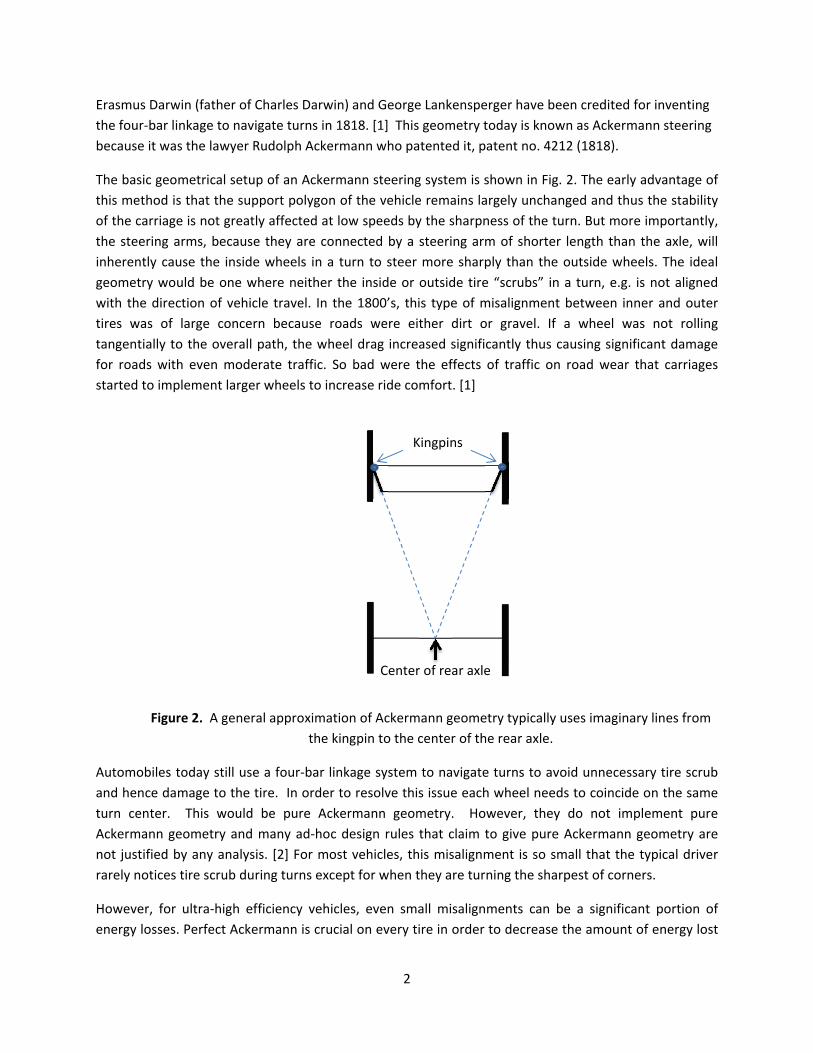
The basic geometrical setup of an Ackermann steering system is shown in Fig. 2. The early advantage of 

this method is that the support polygon of the vehicle remains largely unchanged and thus the stability 

of the carriage is not greatly affected at low speeds by the sharpness of the turn. But more importantly,   

the steering arms, because  they are connected by a steering arm of shorter  length  than  the axle, will 

inherently cause  the  inside wheels  in a  turn  to steer more sharply  than  the outside wheels. The  ideal 

geometry would be one where neither  the  inside or outside tire “scrubs”  in a turn, e.g.  is not aligned 

with  the direction of vehicle  travel.  In  the 1800’s,  this  type of misalignment between  inner and outer 

tires  was  of  large  concern  because  roads  were  either  dirt  or  gravel.  If  a  wheel  was  not  rolling 

tangentially to the overall path, the wheel drag  increased significantly thus causing significant damage 

for  roads with  even moderate  traffic.  So bad were  the  effects of  traffic on  road wear  that  carriages 

started to implement larger wheels to increase ride comfort. [1] 

 

Figure 2.  A general approximation of Ackermann geometry typically uses imaginary lines from 

the kingpin to the center of the rear axle. 

Automobiles today still use a four‐bar  linkage system to navigate turns to avoid unnecessary tire scrub 

and hence damage to the tire.  In order to resolve this issue each wheel needs to coincide on the same 

turn  center.    This  would  be  pure  Ackermann  geometry.    However,  they  do  not  implement  pure 

Ackermann geometry and many ad‐hoc design  rules  that claim  to give pure Ackermann geometry are 

not  justified by any analysis. [2] For most vehicles, this misalignment  is so small that the typical driver 

rarely notices tire scrub during turns except for when they are turning the sharpest of corners. 

However,  for  ultra‐high  efficiency  vehicles,  even  small misalignments  can  be  a  significant  portion  of 

energy losses. Perfect Ackermann is crucial on every tire in order to decrease the amount of energy lost 

Center of rear axle 

Kingpins

3  

due  to misalignment of  the  tire with direction of  travel. Because of  the  low speeds of such ultra‐high 

efficiency  vehicles,  such misalignment has  little  benefit  to  the  overall  vehicle performance,  and only 

produces waste heat.    

2. Ideal Ackerman Geometry 

In this section, the definition of the ideal Ackermann geometry is reviewed briefly, as this geometry will 

be  used  in  later  sections  to  determine  deviations  from  ideal.  Fig.  3  shows  the  relation  between  the 

radius  of  turn  and  the  steering  angles  necessary  for  the  inside  and  outside  tires.  For  this  paper,  an 

“ideal” Ackermann geometry is defined as when the tire is perfectly tangent to a circle drawn from the 

center of  the  turn, e.g. when  tires F and G are perpendicular  to  lines  that  intersect  the center of  the 

turn, as shown in Fig. 3. 

 

Figure 3.  Relationship between δoutside and δinside. 

Looking at Fig. 3, one can see that two triangles are formed that can be used to derive the ideal steering 

angle.    The ideal angle of the outside wheel is calculated using ∆EGH, 

tan 2, 

tan 2

. 1  

The ideal angle of the inside wheel is calculated using ∆EFJ, 

 

WB 

δoutside 

R 

  δideal 

E 

F  G 

H J 

2 

δideal

δoutside

4  

tan2, 

tan2. 2  

This  ideal angle will be used  in  later sections  to calculate  the error between actual and  ideal steering 

geometries. 

3. Four‐Bar Analysis to Derive the Optimal Ackerman Geometry 

For very  low  speed  turns  like  those  seen  in ultra‐high‐efficiency  competitions,  the most  fuel efficient 

four‐bar steering mechanism  is one  that minimizes any  tire scrub. To derive  this geometry,  tire scrub 

forces must be derived from the steering geometry of the four‐bar mechanism, the turn radius, and the 

tire  parameters.    To  simplify  the  analysis  that  follows, we  assume  that  the  tires  are  in  pure  rolling; 

maneuvers are made at a  low speed; wheels have equal static weights and no weight transfer occurs; 

and  all  maneuvers  take  place  on  a  flat  surface.    For  later  numerical  steps  in  this  algorithm,  the 

dimensions  from  the  Penn  State University  entry  are used.  The outside wheel  is  assumed  to  be  the 

driver of the steering mechanism. 

Referring to Fig. 4,  there are two dimensions that govern the  four‐bar arrangement:  the  track  (T) and 

the wheelbase (WB).  The Ackermann design uses a trapezium‐style four‐bar, one that is convenient to 

consider  as  a  first  approach  because  of  symmetry,  e.g.  that  the  analysis  is  not  dependent  on  the 

direction of the turn.   A typical trapezoidal Ackermann geometry can be seen at the top of Fig. 4.   The 

ground link of the four‐bar, R1, is usually connected to a fixed frame and is hereafter assumed to have a  

fixed dimension, T.  The lengths of R2 and R4 are assumed to be the same, but their angles will vary since 

they are dependent on R3 and the Ackermann Angle (AA).  We define the Ackermann Angle, AA, as the 

angle that is formed between the wheel and the steering arm, R2.  Because this angle is mechanically set 

in most steering systems by the inset angle of the steering arm relative to the tire plane, it is hereafter 

assumed  that  the angle AA  remains constant  for a particular set‐up. Consistent with  the definition of 

low‐speed steering, the radius of turn  is defined as the distance from the turn center to the center of 

the rear axle. 

 

 

 

 

 

 

5  

 

 

 

 

 

 

 

   

  

 

 

 

 

 

Figure 4. General representation of four‐bar steering design for vehicles. [3] 

Using the geometry defined previously for the special case when R3 is parallel to R1, R2 can be calculated 

by trigonometric relationships to obtain Eq.(1). 

12sin

3  

We now consider the  ideal Ackermann geometry of each  individual tire constrained by the trapezoidal 

mechanism above. During a turn, the four‐bar can be modeled assuming that the link R2 (connected to 

the outside tire) is the “driver” of the mechanism, and thus that the angle of the tire connected to R2 is 

assumed to be set up to have perfect Ackerman geometry.  In order to optimize the four‐bar, we seek to 

solve for the angle of link R4 in order to minimize scrub on the inside tire.  

Using ∆ABD, the length of triangle side, e, is given by 

2 cos  

2 cos 4  

D’     A’ 

2 

B’ 

 

R2 

R1 

e 

D’ 

B’ 

 

 

  C’  

 

 

e 

AA 

A D 1

C B

R1

R2

R3

R4

Front of Vehicle

Outside Wheel  Inside Wheel 

 

6  

The length, e, can then be used to obtain the angle α in ∆ABD, which is used later. 

sinsin

 

sinsin

5  

We now relate the above geometries to ∆BCD in order to calculate the angle of the inside wheel. First, 

the length e is used to calculate ,  

2 cos  

cos2

6  

sin sin 

sinsin

. 7  

The  steering angle of the inside wheel can now be found.  When the wheels are straight, 

90°, 8  

and we also know that α and β change as a function of the driving link.  Because the angle, AA, remains 

constant, the steering angle of the inside and outside wheel can now be found: 

| 90°| 9  

90°. 10  

4. Determination of Ackermann error 

Using the previous equations, one can find the orientation error between the  ideal angle of the  inside 

tire, and the actual angle of the  inside tire, for a variety of steering conditions that define the angle of 

the outside tire. For a given steering geometry, one can sweep through the possible steering angles of 

the  outside wheel  to  calculate  all  possible  angles  of  the  inside wheel  for  comparison  to  ideal.  The 

limiting angle is one that causes the four‐bar to reach its lock point, e.g. when the following condition is 

met. 

11  

 After the four‐bar reaches  its  lock point the four‐bar becomes unpredictable.   The four‐bar equations 

are only used to calculate the position of the wheels in a left hand turn since the results for a right hand 

turn would be the same.   

7  

Once all steering angles are known, the misalignment error in the inside tire is calculated by comparing 

the inside steer angle, δideal, with the actual inside steer angle caused by the four‐bar linkage.  

100 12  

This calculation is done for a wide range of four‐bar set‐ups and each four‐bar is rotated to the point of 

lock.   

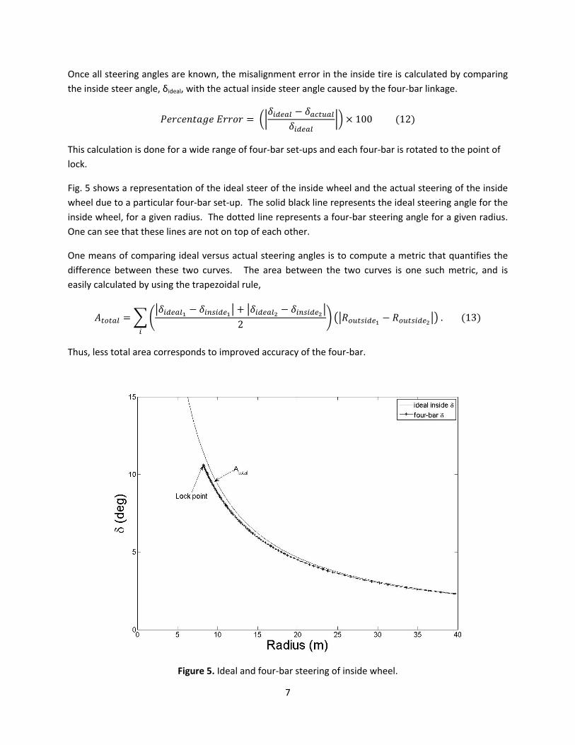
Fig. 5 shows a representation of the ideal steer of the inside wheel and the actual steering of the inside 

wheel due to a particular four‐bar set‐up.  The solid black line represents the ideal steering angle for the 

inside wheel, for a given radius.  The dotted line represents a four‐bar steering angle for a given radius.  

One can see that these lines are not on top of each other.   

One means of comparing  ideal versus actual steering angles  is to compute a metric that quantifies the 

difference between  these  two  curves.     The area between  the  two  curves  is one  such metric, and  is 

easily calculated by using the trapezoidal rule, 

2. 13  

Thus, less total area corresponds to improved accuracy of the four‐bar. 

 

 

Figure 5. Ideal and four‐bar steering of inside wheel. 

8  

 

 

Figure 6. Atotal associated with four‐bar design  

Fig. 6 shows the accuracy of different four‐bar set‐ups with relations to perfect Ackermann steering for a 

track width of 0.6255 meters and vehicle  length of 1.6 meters. The surface plot shows  that  there  is a 

relationship between R3 and the AA that gives improved steering, and the plot also shows that there is 

no trapezoidal steering geometry that gives an ideal geometry over all turn radii.  

Considering the best‐case geometry for each length of R3, one obtains the plot as shown in Fig. 7.  Also 

seen  in this figure  is the  linear fit, showing that the relationship between R3 and the  ideal Ackermann 

Angle of the steering arm is approximately, but not quite, linear. 

 

Figure 7. Minimum value of Atotal represents valley from Fig. 6 for each four‐bar setup. 

9  

One common method to establish the trapezoidal geometry  in practice  is to project an  imaginary  line 

from  the  steering arms  to  the center of  the  rear axle, and  then  to use a  trapezoidal configuration  to 

connect these arms.  If one uses this rule of thumb,  one obtains an AA angle of 11.05°.  Looking at Fig. 7 

we see that the ideal four‐bar setup for this rule of thumb only occurs when the steering arm length is 

roughly 0.3 meters. For all other configurations, this design rule is not ideal.  

5. Optimization of Steering Geometry for a Particular Driving Course 

The  previous  error  analysis  considered  a  cumulative  error  that  weights  all  steering  angles  equally. 

However,  vehicles  in  competition  are  not  required  to  have  extremely  tight  turning  geometries  nor 

encounter all  radii  turns with equal  frequency. A more appropriate approach would be  to weight  the 

errors of common turn geometries most heavily, and to give little or no weight to turns that are rarely if 

ever encountered. 

The Shell Eco‐marathon Americas track at the Discovery Green Park has multiple turns of different radii 

and  lengths.   Using satellite  images  from Google maps,  the preferred and most common path around 

the track was traced.  The radius and arc length of each turn is then calculated, and the total length of 

one  circuit was  also  calculated.    The pie  graph  in  Fig.  8  illustrates  the weighted  importance of  each 

particular  turn,  as  determined  by  the  total  arc  lengths  of  each  radii  turn.  Because  the  competition 

vehicle  travels  at  a  nearly  constant  velocity,  even  around  turns,  the  following  histogram  is  also 

representative of the cumulative time the vehicle spends within each turn. 

 

Figure 8.  Weighted relationship of distance in straightaway and radii (m) of turns. 

Using the pie graph and modeled four‐bar analysis, we can then re‐weight the results shown previously 

by the factors given in Fig. 6. Specifically, the  steering differences for the four‐bar and ideal steer angle 

of each turn are multiplied by the corresponding weight.  

| | 14  

4%

10%1%

7%2%

10%66%

30.88 36.90 46.74 65.72 77.00 77.80 Straightaway

10  

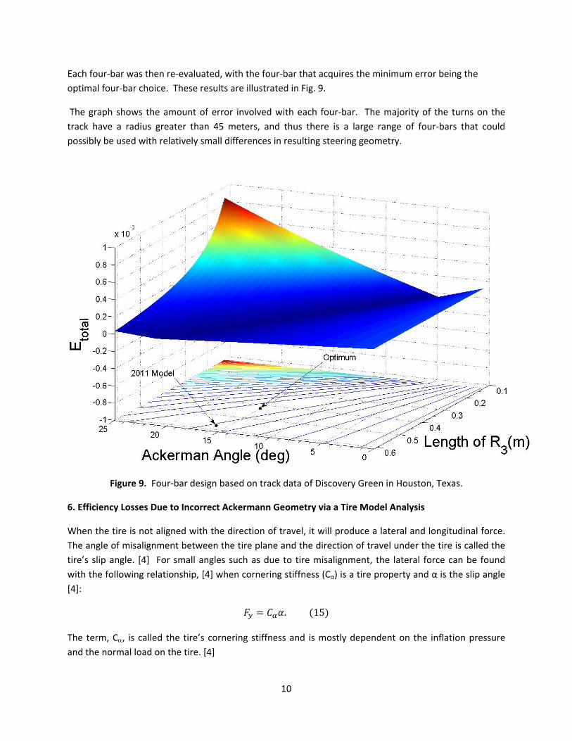
Each four‐bar was then re‐evaluated, with the four‐bar that acquires the minimum error being the 

optimal four‐bar choice.  These results are illustrated in Fig. 9.  

 The graph shows  the amount of error  involved with each  four‐bar.   The majority of  the  turns on  the 

track  have  a  radius  greater  than  45 meters,  and  thus  there  is  a  large  range  of  four‐bars  that  could 

possibly be used with relatively small differences in resulting steering geometry. 

 

 

Figure 9.  Four‐bar design based on track data of Discovery Green in Houston, Texas. 

6. Efficiency Losses Due to Incorrect Ackermann Geometry via a Tire Model Analysis 

When the tire is not aligned with the direction of travel, it will produce a lateral and longitudinal force. 

The angle of misalignment between the tire plane and the direction of travel under the tire is called the 

tire’s slip angle.  [4]   For small angles such as due  to  tire misalignment,  the  lateral  force can be  found 

with the following relationship, [4] when cornering stiffness (Cα) is a tire property and α is the slip angle 

[4]:   

. 15

The  term, C,  is called  the  tire’s cornering stiffness and  is mostly dependent on  the  inflation pressure 

and the normal load on the tire. [4] 

11  

To understand the  impact of steering misalignment, the following analysis considered the competition 

entry  from  the Penn State  team  in 2010.   The  total weight of  the  car and driver  for Penn State was 

117.02 kg, producing about 1.148 kN of force.   Assuming the weight to be evenly distributed across all 

wheels results  in a normal  load of 0.3826 kN on each wheel.   These tires were operated at a value of 

5.17 bar.  Using Pacejka’s “magic formula” a value of cornering stiffness can be calculated, [5] 

° sin 2 tan . 16  

In order to calculate  , Michelin provided the Pacejka model coefficients for radial ply 45‐75R16 in as 

shown Table 1, tires that were used in competition.   

 57.806  15.101  ‐0.082  0.186 

Table 1.  Cornering Stiffness Coefficients for Michelin radial ply 45‐75R16.  

It  is  recommended  that  the  coefficients only be used  if  the operating  conditions are  in  the  following 

limits:   0.3 < Fz < 0.6 kN and 4 < P < 6 bar, which the competition vehicle followed. [6]   The cornering 

stiffness was calculated to be 5696 N/rad. 

The  cornering  stiffness, ,  measurement  enables  a  fuel  mileage  analysis  of  the  Ackermann 

misalignment.  From  previous  Penn  State  power measurements,  it was  determined  that  the  vehicle 

overcomes a steady drag force of 17.15N averaged over each lap in order to maintain a constant speed 

of 24.14 kph.   From  the  tire model mentioned before, one can calculate  the  lateral  force  involved  in 

cornering by considering the elapsed time in each part of the track. Because the vehicle was moving at a 

constant speed, the weights that were previously calculated can be used.   

For  each  turn,  the misalignment  errors  in  each  turn were  calculated  based  on  the  specific  four‐bar 

configuration of each turn.  Equation (17) yields the decrease in fuel mileage per run. 

∑

17  

Fig. 10 shows the  loss  in fuel mileage relative to the measurements obtained at competition, due to a 

particular  four‐bar  arrangement.    One  can  see  the  importance  of  four‐bar  geometry  and  how  tire 

misalignment  affects  fuel mileage.    Choosing  the  optimal  four‐bar  from  Fig.  10,  the  vehicle  would 

theoretically  lose  0.1771 MPG.    For  the  actual  geometry  used  in  the  competition  vehicle  and  the 

measured  fuel  economy  of  4700 MPG,  the  loss  due  to  the  current  four‐bar  set‐up,  50.0 MPG,  only 

penalizes  the vehicle 1.1%.   While this seems small, one must recognize that past competition entries 

have  lost  ranking based on  smaller amounts, which can be particularly  frustrating given  that  steering 

geometry is easily adjusted to the ideal value with no vehicle redesign. 

 

12  

 

Figure 10.  Loss in fuel efficiency based on the four‐bar geometry 

5. Conclusions 

This paper considered the fuel losses associated with the misalignment of the front steering geometry 

due to the typical trapezoidal Ackermann geometry setup. Starting with a standard front steering 

geometry, an algorithm was developed to calculate the optimal four‐bar geometry for a vehicle and it is 

seen that such geometries can approach, but never reach, perfect Ackermann geometry  on all 

individual tires simultaneously for low‐speed turns.  Using turning data collected from prior 

competitions, predicted performance improvements were given for Penn State’s super‐high‐mileage 

entry in the Shell Eco‐marathon Americas.   

A result of this analysis is the realization that the only way to have perfect Ackermann is to steer each 

wheel independently, which may be possible by using a servo motor.  This could be a costly endeavor 

and more than likely result in extra weight added to the vehicle with more energy consumed to initially 

get the vehicle up to speed and to maintain the vehicle at a steady speed.  This perpetual tradeoff 

between vehicle weight versus performance is the central problem of ultra‐high‐efficiency vehicle 

challenges.  

Additionally, this analysis ignores the weight transfer would affect how the tire tracks along a given 

radius.  Future work could consider this effect by specifically examining the cornering coefficients of the 

tires and correcting for this accordingly. Another interesting analysis would be to compare the fuel 

economy losses for higher‐speed vehicles, ones where low‐speed approximations are not necessarily 

valid. While faster speeds will cause larger power losses for a given misalignment, the high speeds also 

generally involve much smaller turn radii. Thus, it is unclear whether a 1.1% improvement in fuel 

economy could be expected through optimized steering geometries. 

13  

References: 

[1] D. King‐Hele, "Notes and Records of the Royal Society of London," Erasmus Darwin's Improved 

Design for Steering Carriages‐and Cars, vol. 56, no. 1, January 2002.  

[2] W. F. Milliken and D. L. Milliken, Race Car Vehicle Dynamics, Warrendale, PA: Society of Automotive 

Engineers, Inc., 1995.  

[3] H. Sommer, "ME 481 Computer‐Aided Analysis of Mechanical Systems," [Online]. Available: 

http://www.mne.psu.edu/sommer/me481/notes_03_01.doc. [Accessed 13 March 2011]. 

[4] J. C. Dixon, Tires, Suspension, and Handeling, Warrendale, PA: Society of Automotive Engineers, Inc., 

1996.  

[5] P. H.B., Tyre and Vehicle Dynamics, Oxford: Butterworth and Heinemann, 2002.  

[6] J. J. Santin, The World's Most Fuel Efficient Vehicle:Design and development of Pac Car II, Zuric, 

Singen: vdf Hochsch.‐Verl. ETH, 2007.