Optical Trapping

MIT Department of Physics

An optical trap or “optical tweezers” is a device which can apply and measure piconewton sized forces on micron sized dielectric objects under a microscope using a highly focused light beam. It allows very detailed manipulations and measurements of several interesting systems in the fields of molecular and cell biology and thus acts as a major tool in biophysics. They are used in biological experiments ranging from cell sorting to the unzipping of DNA. Similar principles are also used in physical applications such as atom cooling. In this experiment, you will measure the Brownian motion of a trapped silica microsphere in aqueous solution, both testing the theory of statistical mechanics and calibrating the “spring constant” of the trap. Then, using the calibrated trap, you will measure forces in biological systems, such as the actin-myosin molecular motors of vesicle transport in onion cells, the E. coli flagellar motor, or the restoring force of a stretched DNA molecule.

In its present form, large portions of this lab guide are derived from the literature for MIT Bioenhineering subject 20.309 [1] and UC Berkeley Physics subject Physics 111 Lab [2].

PREPARATORY QUESTIONS

1. In the limit of ray optics, the trapping force ona dielectric sphere can be understood as arisingas a reaction force to the change in linear mo-mentum experienced by refracted light rays. Tobetter understand how the scattering and gradientforces — and the trap’s stability — vary withdisplacement from the trap center both verticallyand horizontally, spend some time exploring thisJava applet simulator developed by the lab ofRoberto DiLeonardo, CNR-IPCF Dipartimento diFiscica, Universita di Roma Sapienza in Italy[3]. Describe and qualitatively sketch how adielectric sphere slightly displaced from the centerof a stable trap experi-ences a restoring force. Isthe center of the trap at the same location as thefocus of the light? Explain why high numericalaperature optics are used in the experiment.Finally, given the wavelength of the laser andthe sizes of objects to be trapped in thisexperiment, do you trust the ray opticssimulation to be quantitatively accurate?

2. Estimate the time and distance required for a mo-bile bacteria of typical bacterial speed in an aque-ous environment to come to a halt under viscousdrag. See the seminal work of Purcell (1976) [4].How do these time and length scales compare tobiologically relevant scales? How does ma compareto the force needed to keep the bacteria moving atits initial constant speed (before it stopped), wherea is the average deceleration of the bacteria, and mis its mass?

3. What are the principle safety hazards you couldencounter in this experiment? How do you avoiddanger from these hazards?

SUGGESTED SCHEDULE

Day 1: Familiarize yourself with the apparatus. Make detailed notes on the effects of each control knob. Prepare an appropriate sample and trap a micro-sphere.

Day 2: Calibrate the QPD voltage to stage position us-ing a fixed bead sample. Measure Brownian noise on a floating bead to obtain data for equipartition and PSD analysis. Obtain a first estimate of Boltz-mann’s constant and trap stiffness.

Day 3: Make an onion cell sample and trap a vesicle.

Day 4: Finish onion cell experiment. Optionally, do Stokes drag measurement — to refine Boltzmann’s constant — or further biological experiments. Note that biological samples may take days to prepare, so you must plan ahead and communicate with your instructors.

The experimental goals are:

1. Measure Boltzmann’s constant using equipartitiontheorem and Brownian PSD

2. Calibrate optical trap stiffness versus laser supplycurrent

3. Estimate force and speed of molecular motorstransporting vesicles in onion cells

I. INTRODUCTION

Light can impart a force, due to the fact that photons carry momentum. These forces are very small compared with those typical in the macroscopic world, but they can be very large relative to typical forces on single atoms, molecules, and small biological organisms, at the microm-eter and nanometer scale. Focused laser beams can se-lectively impart force to atoms, to cool them from room

Id: 51.opticaltrap.tex,v 1.11 2012/02/06 23:45:01 spatrick Exp spatrick

2 Id: 51.opticaltrap.tex,v 1.11 2012/02/06 23:45:01 spatrick Exp spatrick

temperature to a few micro-Kelvin and below. They can also be used to push or trap microscopic dielectric spheres — or even entire, living, cellular organisms, inside bio-logical media.

The method of optical trapping was discovered by Arthur Ashkin in 1970 [5] [6]. He calculated that the ra-diation pressure from a high power laser, focused entirely onto a micron-sized bead (or “microsphere”), would ac-celerate the bead forward at nearly 106 m/s2 . When he performed the experiment to test this prediction, he found that while the target bead was indeed accelerated downstream, other beads in the solution were attracted laterally into the beam-path from other parts of the sam-ple. He then created the first working optical trap by us-ing two opposing laser beams. At one point a bacterium that had contaminated a sample became trapped in the beam, thus instigating the trap’s revolutionary use in cell biology. Today optical traps are used extensively in both atom-trapping experiments and in biophysics labs world-wide.

In this laboratory experiment, you will explore the use of optical forces to trap dielectric microspheres held within a thin layer of water and vesicles in onion cells. The typical mechanical forces involved are on the scale of piconewtons (10−12 N). Relative to this scale, hydrody-namical forces (drag and diffusion) on the microspheres and vesicles are substantial. Thus, the optical trap pro-vides an excellent opportunity to study the physics of Brownian motion, which you will use to obtain a quan-titative measurement of Boltzmann’s constant. In the process, you will calibrate the dependence of trap stiff-ness (force/distance) on laser supply current. Biologi-cal motors, which are vital to intracellular transport and bacterial locomotion, also act with forces on this scale. You may thus employ the optical trap to quantify the speed and force of a molecular motor moving a vesicle along an actin fiber in an onion cell.

I.1. The Physics of Optical Trapping

The following material in this subsection is taken nearly verbatim from UC Berkeley’s Junior Lab guide on their optical trap experiment [2]. The most straightforward mechanism to understand

the physics of trapping is to consider the change in mo-mentum of light that is scattered and refracted by the dialectic material, in our case a silica glass bead. Any change in the direction of light imparts momentum to the bead. This mechanism holds for objects much larger in diameter than the wavelength of the laser. A ray-tracing argument implies that the scattered light creates a scattering force in the direction of light propagation, while the refracted light creates an opposing gradient force. When the bead is in the center of the trap, these forces cancel. When a bead moves slightly away from the center, a net force is applied towards the center, making this a stable equilibrium.

FIG. 1. A ray diagram showing how the gradient force stabi-lizes the trap laterally

In order to understand how the equilibrium is stable, it will help to consider how the gradient force responds to displacement of a bead from the center. As seen in Figure 1, the red region represents the “waist” of the laser at its focus point, with the laser passing upward through the sample chamber. The blue ball is the bead, and the dark red arrows (1) and (2) represent light rays whose thicknesses correspond to their intensities (note that the beam is brightest at its center). In case (a), with the particle slightly to the left of center, the two rays refract through the particle and bend inwards. The reactionary force vectors, F1 and F2, of each ray on the bead are shown as black arrows. Because ray (2) is more intense (and thus carries more momentum) than ray (1), the net force on the bead is to the right. Thus, a perturbation to the left causes a rightward-directed force back towards the trap’s center.

In case (b) the particle is centered laterally in the beam and will not be pushed left or right. The net gradient force is downward, which is balanced by an upward scat-tering force (not shown) due to reflection of some of the light.

To better understand how the scattering and gra-dient forces and the trap’s stability vary with bead displacement both vertically and horizontally, try this Java applet from the DiLeonardo lab [3] in Italy. The model used for this ap-plet shows the importance of a high numerical aperture lens, as the extremal rays illustrated contribute dispro-portionately to the change in gradient force vertically.(Note that you must adjust the numerical aperture at the bottom of the applet in order to obtain a stable trap.) By moving the bead around and looking at the net force vec-tor, you can get a pretty good feel for how the restoring force varies as a bead is displaced horizontally or verti-cally from the trap’s center. Note particularly how the trap is less stiff as the bead is displaced above the trap’s center. Remember this when you trap your first bead and try moving the bead with the stage controls.

3 Id: 51.opticaltrap.tex,v 1.11 2012/02/06 23:45:01 spatrick Exp spatrick

The ray optics approach described above holds for trapped objects whose diameter is much larger than the wavelength of the laser. For objects much smaller than this wavelength, ray optics are not valid. In this case, conditions for Raleigh scattering are satisfied and the object can be treated as a point dipole. The scattering force then is due to absorption and reradiation of light by the dipole, and the gradient force arises from the in-teraction of the induced dipole with an inhomogeneous electromagnetic field. This mechanism is detailed in the Neuman and Block review [7] and the Wikipedia article on optical trapping (http://en.wikipedia.org/wiki/ Optical_tweezers). Since the 1 micrometer diameter beads we use in this lab essentially match the 975 nm wavelength of our laser, neither of these mechanisms is quite right. More complicated electromagnetic theories have been invoked to account for the observed forces [7] [8] [9]. However, these theories are not particularly useful in calculating forces from first principles; the ray optics approach is useful for guiding trap design and beam align-ment, while calibration is based on direct measurements of bead motion.

I.2. Boltzmann’s Constant and the Equipartition Theorem

The macroscopic world of masses and gasses con-nects to the microscopic world of atoms and parti-cles through the laws of thermodynamics. It is in many ways remarkable that a collection of particles at some temperature T gives rise to a macroscopic pres-sure P , when confined within a volume V , where a single constant relates the number of particles n to the total kinetic energy of the gas. This constant is Boltzmann’s constant (http://en.wikipedia.org/ wiki/Boltzmann%27s_constant), kB , and the relation-ship is the ideal gas law, PV = nkB T . How can one measure Boltzmann’s constant? The crux

of this challenge is the problem that it is unrealistic to be able to count the number of particles in a typical vol-ume of gas. Thus, a direct approach based on the ideal gas law is difficult. However, the intrinsic connection between kinetic energy and temperature is also revealed through the fluctuations of the force imparted by the gas. The equipartition theorem, which is fundamental to thermodynamics, holds that each degree of freedom in a

1physical system at thermal equilibrium will have kB T2 of energy. A single particle trapped in a harmonic po-

1tential — i.e., a mass on a spring — has energy αx2 ,2 where α is the spring constant, and x is the particle’s dis-placement from the trap center. At thermal equilibrium with temperature T , such a trapped particle would have average energy

1 αhx 2i = 1

kB T (1)2 2

according to the equipartition theorem. Here, hx2i is the

statistical variance in the position of the particle, result-ing from the fluctuation of the position of the particle due to random (Brownian) motion imparted by the medium at temperature T with which the particle is in thermal equilibrium. If α and T were known, and if hx2i were measured, for example, by microscopic observation of the Brownian motion of a single particle, then Boltzmann’s constant kB could be determined. This is exactly what we will accomplish in this experiment.

I.3. Brownian Motion and the Power Spectral Distribution (PSD) Function

The theory of Brownian motion predicts not only the variance of the trapped particle’s position with time, but also the spectrum of these variations. Model the effect of the buffeting of the particle by a thermodynamically large number of individual molecules of the medium as a random time-dependent force F (t). If each impact is truly random and uncorrelated, as one would expect from a gas of particles at thermal equilibrium, then the corre-lation time of the random forcing should be very short. Approximating it as zero, the resulting spectrum of the force is “white noise”. Further approximating the mo-tion of the bead as completely overdamped (that is, the viscous forces dominate over the inertia, known as the regime of low Reynolds number), the position x of the bead in the harmonic optical trap of stiffness α is gov-erned by the equation of motion

βx+ αx = F (t), (2)

where β is the hydrodynamic drag coefficient β = 3πηd, d is the bead diameter, and η is the viscosity of the medium.

Using the Wiener-Khinchin theorem to define a “power spectral distribution” function (PSD) or “power spec-trum” via the Fourier transform of the time-averaged autocorrelation function, the result is s

kB T Sxx(f) = , (3)

π2β(f2 + f2)0

where f0 = α/2πβ. Note, this power spectrum, √ with units of length/ frequency, is different from, but closely related to the power spectrum defined as the com-plex norm of the Fourier transform, with which you may be more familiar. We have used the result that the power √ spectrum of the white noise is 4βkB T [10].

I.4. Molecular Motors and Forces in Microbiology

In this experiment, you will measure piconewton scale forces associated with the motion of individual (but large) molecules in microbiological systems. Organelles are transported over relatively large

distances within cells by myosin motors that step

4 Id: 51.opticaltrap.tex,v 1.11 2012/02/06 23:45:01 spatrick Exp spatrick

along actin microfiber filaments. For further back-ground specific to our model system (vesicle trans-port in onion epidermal cells), see the writeup in UC Berkeley’s Physics 111 lab guide [2] on onion cell biophysics.

You may also have the opportunity to perform mea-surements on further biological systems. The rotating flagellar motor of the famous bacteria Escherichia coli (E. coli for short) is a macromolecule whose rotational speed and torque are well suited to measurement in our optical trap. Further background on this system can also be found in the UC Berkeley’s Physics 111 lab guide [2] and references therein.

A final system you may be able to measure, with enough time and fortitude, is the mechanical (spring-like) properties of the DNA molecule. You may be fa-miliar with the freely-jointed chain model from introduc-tory statistical mechanics. In that system, a set of links in a chain are allowed to take any orientation with re-spect to the previous link, with no cost in energy. De-spite the fact that there is no energy cost associated with bending any link, there is still a macroscopic force that resists stretching the system as a whole, due to the enor-mous entropy of crumpled configurations as compared to straightened configurations. That is, the macroscopic system at finite temperature T will tend towards con-figurations that minimize the free energy F = U − T S, where U is the internal energy and S is the entropy. In the case of the freely-jointed chain, U = 0 so minimizing the free energy gives rise to forces which are entirely en-tropic in nature. (Curiously, in this model, adding heat causes the system to shrink.) The real DNA molecule has a finite bending stiffness, giving an internal energy which prefers straighter configurations. The competition between energy and entropy leads to regimes of behavior where the net macroscopic force is dominantly “entropic” and others where it is dominantly “enthalpic”. This is captured in the so-called worm-like chain (http://en. wikipedia.org/wiki/Worm-like_chain) model, which is well described on Wikipedia.

II. APPARATUS

The MIT Junior Lab optical trap setup is based on an inverted microscope with a fiber-coupled infrared laser source, and a quadrant photodetector for posi-tion sensing, as described in a very nice paper au-thored by students and faculty in the MIT Department of Biological Engineering [11]. The Junior Lab appa-ratus was assembled from a kit, available from Thor-labs (http:// www.thorlabs.com/NewGroupPage9.cfm?

FIG. 2. Photograph of the Optical Trap apparatus, show-ing the paths of the laser (red) and visual illumination LED (blue).

ObjectGroup_ID=3959), and designed by Steven Wasser-man of the MIT Department of Biological Engineering.

The main purpose of the setup is to provide an intense, tightly focused laser beam at a desired position, within a thin fluid sample cell containing particles or biological organisms. The setup also allows visual imaging of the sample cell, and quantitative measurement of the posi-tion of the particles based on the deflection angle of laser light.

II.1. Light Sources

There are two light sources involved in the apparatus: a 975 nm laser used for trapping and measurement, and a white LED used for visual observation of the sample.

II.1.1. Laser and Laser Beam Path

The main light source for the optical trap is an intense 330 mW diode laser (http://en.wikipedia.org/wiki/ Laser_diode) producing coherent 975 nm (infrared) light (http://www.thorlabs.com/thorProduct.cfm? partNumber=PL980P330J). This wavelength is chosen

5

© AIP Publishing LLC. All rights reserved. This content is excluded from our Creative Commons license. For more information, see https://ocw.mit.edu/help/faq-fair-use.

FIG. 3. Schematic diagram of the optical beam paths in the optical trap apparatus. Based on a similar diagram from [11].

because it is sufficiently far from typical absorption lines in biological specimens; in addition, relatively inexpen-sive laser diodes are available at this wavelength, because of its use in pumping the erbium doped fiber amplifiers (http://en.wikipedia.org/wiki/Erbium-doped_ fiber_amplifier#Erbium-doped_fiber_amplifiers) used in modern optical telecommunication systems. The laser is packaged with an integrated optical fiber, through which the laser light is delivered to the setup. The laser must be operated at a stable temperature, since changes in its temperature can significantly change the output wavelength (by ∼10 GHz/deg C). The output power of the laser is controlled by its current, which can range between ∼100 mA and ∼400 mA, roughly corresponding to 0 mW to 330 mW. The trapping force is determined by the intensity of the laser beam, and thus the current must be very precisely controlled to maintain a stable trap.

As shown in Figure 3, the laser light is collimated in a FiberPort micropositioner (L5), then passed through two lenses (L4 and L3) to expand it. The beam is then re-flected by a “hot mirror,” (http://en.wikipedia.org/ wiki/Hot_mirror) (DM1) which reflects infrared wave-lengths, but is transparent to visible wavelengths. The light then bounces off a 45 degree turning mirror (M45) and passes up through a Nikon 100X oil immersion objec-tive (CDI4390; the “lower objective”), which focuses the beam to a tight 1.1 µm focus, at a position between the cover slip and the glass slide, where particles (or biolog-

Id: 51.opticaltrap.tex,v 1.11 2012/02/06 23:45:01 spatrick Exp spatrick

ical specimens) are suspended in liquid. The laser light scattered off the sample passes upward through another Nikon objective, used as a condenser (CDI4391; the “up-per objective”), which collects the light. This collected light is then reflected off another hot mirror (DM2), into a lens (L1) which images the back plane of the condenser onto a quadrant photodetector (QPD). A neutral density filter (ND) is used to attenuate the light incident on the QPD.

II.1.2. White Light LED and Sample Visualization

White light generated by a simple light emitting diode (LED) is used for visualizing the sample. The white light passes through a hot mirror (DM2) and down through the upper objective, onto the sample. The light transmitted through the sample is then collected by the lower objec-tive, bounced off the bottom mirror (M45), and passed through another hot mirror (DM1). Any stray infrared light is then separated from the visible white light with a filter (KG and/or OG), and focused with a lens (TL), and bounced off a turning mirror, into a CCD camera.

II.2. Inverted Oil Immersion Microscope

The microscope at the center of this apparatus is com-prised of two objectives and the sample; these are de-scribed below. A precise stage, which is also essential to the microscope, is described in the next subsection.

The two objectives in this microscope focus laser light onto the sample to provide the optical trap, and also provide magnification used for visual observation of the sample. They are configured with positions inverted from the more traditional configuration; the magnifying / fo-cusing objective (here, called the “lower objective”) is placed below the sample. In addition, the lower ob-jective is an oil immersion (http://en.wikipedia.org/ wiki/Oil_immersion) objective; it is designed such that a drop of oil, placed on top of the objective, is used to in-crease the numerical aperture (http://en.wikipedia. org/wiki/Numerical_aperture) of the lens. This in-creases the amount of light which it gathers, and also reduces the waist of the focused laser beam. The up-per objective is an air spaced infinity condenser, which delivers bright field (http://en.wikipedia.org/wiki/ Bright_field_microscopy) illumination from the white LED, and also collects scattered laser light from the sam-ple for beam position detection.

II.3. Position Measurement

The key to quantitative measurements in the optical trap apparatus is precise knowledge of two positions: that of (1) the sample, and (2) the laser beam. The position of the sample is determined by the microscope stage. The

6 Id: 51.opticaltrap.tex,v 1.11 2012/02/06 23:45:01 spatrick Exp spatrick

FIG. 4. Photograph of the upper and lower objectives of the trap apparatus, showing the sample mounted in between.

position of the laser beam, after scattering off the sample, is determined by the quadrant photodetector.

II.3.1. Quadrant Photodetector (QPD)

The QPD is a semiconductor photodiode (http://en. wikipedia.org/wiki/Photodiode) which is segmented into four parts. An electric circuit embedded with the QPD, with difference amplifiers, computes differences be-tween the four segments. By virtue of the linearity of the detector, the differences thus provide information about the position of a uniform intensity light beam, incident on the detector, relative to the center of the photodiode. When the beam is perfectly centered, all the differences cancel, giving zero output voltage. When the beam is dis-placed up or down, the vertical axis output amplifier goes positive and negative, correspondingly; similarly, left and right displacements of the beam produce corresponding positive and negative voltages in the horizontal voltage output. Given a known beam displacement, the hori-zontal and vertical output voltages of the QPD can then be translated into distances. The QPD responds to po-sition changes fairly quickly, within less than ∼100 µs, and thus is particularly useful for quantitative measure-ment of phenomena happening at frequencies up to ∼10 KHz. This time scale includes the regime of fluctuating Brownian motion of particles, which we wish to observe, and which would be inaccessible using only the slow ∼30 Hz frame rate of the CCD video camera.

II.3.2. Microscope Stage

The microscope stage has three axes of adjustment, and includes both manual and electrical control of the stage position. The manually adjustable microme-ters (Thorlabs DRV002 (http://www.thorlabs.com/

FIG. 5. Schematic of a quadrant photodetector. © University of Oxford. All rights reserved. This content is excluded from our Creative Commons license. For more information, see https://ocw.mit.edu/help/faq-fair-use.

FIG. 6. Photograph of the trap setup, showing the microm-eters for adjusting the stage position, and the turnscrews for adjusting the QPD beam position.

thorProduct.cfm?partNumber=DRV002)) have both coarse and fine (“differential”) adjustment knobs, and an overall travel range of 4 mm. Be careful to keep the fine adjustment knob within range (do not completely unscrew it, as the knob may fall off and the interior bearings may be damaged). For adjustments beyond 4 mm, the sample may be moved under the spring clips, or the entire microscope stage can be pushed back and forth on the small translat-ing breadboard upon which it is mounted. Note the definition of the X, Y, and Z axes, as shown in Figure 6.

The position of the sample can also be controlled precisely using piezoelectric actuators (http://en.

7

FIG. 7. Block diagram of the control electronics used in the MIT Junio Lab optical trap system.

wikipedia.org/wiki/Piezoelectric) which are built into the microscope stage. These piezo actuators are driven by high voltage controllers based on feedback from strain gauges (http://en.wikipedia.org/wiki/ Strain_gauge) also built into the stage. The strain gauges provide a voltage output which can be converted to displacement of the stage; the conversion factor can be determined by the procedure described in the next section.

II.4. Control System and Electronics

The optical trap system as diagrammed in Figure 7 is controlled by a set of modular electronics, comprised of the computer, the CCD camera, the Thorlabs T-cube stage piezo and quad photodetector controllers, and the NIDAQ USB-622 interface box. The computer, running Matlab, is connected by USB to the CCD camera, the NIDAQ USB-622, and the T-cube blocks. Digital video from the CCD is presented to allow visualization of the sample. The NIDAQ box digitizes four analog voltages (Ain0 through Ain3), which represent the stage X and Y positions (measured by the strain gauges attached to the X and Y piezos embedded in the stage), and the position of the scattered laser beam (measured by the quad photodiode). Analog feedback loops are used to control the piezo voltages to allow precise positioning of the stage, with sub-micrometer accuracy. The NIDAQ box also provides two analog output voltages (Aout0 and Aout1), which allow the computer to control the stage X and Y positions, within the range of the piezoelectric actuator (20µm). The T-cube boxes, as shown in Figure 8, display the

voltages used to drive the piezos, as well as the voltages measured by the strain gauges. By pressing the “mode” button on the strain gauge controllers, the displays on those boxes can be switched to display calibrated position displacement, instead of strain gauge voltage. Use this

Id: 51.opticaltrap.tex,v 1.11 2012/02/06 23:45:01 spatrick Exp spatrick

FIG. 8. Photograph of the stage position and quadrant pho-todetector displays on the T-cube blocks.

feature to determine the conversion between strain gauge voltage and true positional displacement. The QPD con-trol box also has a display, which coarsely shows the X, Y position of the scattered laser beam. This can be useful for coarse alignment of the laser to center it on the QPD.

III. SAMPLES

Three kinds of samples — all placed on microscope slides — are used in this experiment: an aqueous solu-tion of floating silica microspheres, a similar sample with the microspheres fixed to the coverslip, and one or more biological samples, such as onion cells. The geometry and contents of the samples are described below. The proce-dure for preparing samples is described in Appendix A.

III.1. Sample Geometry (Flow Channel)

Most of the experiment is performed using a simply prepared flow channel configuration. The sample is a thin layer of liquid (typically deionized water or a 1 molar NaCl/water solution) in which particles (1-3 µm diame-ter silica spheres) or biological specimens are suspended. This suspension must be thin in order for the trap light to pass through largely unimpeded and to present a two-dimensional medium for trap operation. Furthermore, the sample must be located very close to the top of the lower objective, to maximize the numerical aperture.

As shown in Figures 9 and 10, the sample is thus constructed from a thin (No. 1.5) cover slip (http: //en.wikipedia.org/wiki/Cover_slip) positioned be-low a standard glass slide with double-sticky tape. This provides a sample volume of about 15 µL. The slide is loaded onto the microscope with the cover slip facing down, towards the lower objective.

III.2. Fixed Microsphere Sample

The fixed bead sample contains 3.21 µm diameter (or other diamater of interest) silica (SiO2) beads which are stuck to the coverslip by virtue of the NaCl buffer so-lution which shields the intrinsic surface charge of silica that would normally repel the beads from the glass sur-face. The beads should be spaced apart from each other by more than 10 µm to avoid signal interference.

8 Id: 51.opticaltrap.tex,v 1.11 2012/02/06 23:45:01 spatrick Exp spatrick

FIG. 9. Photograph of a sample cell, showing the coverslip attached to a glass slide with double-sticky tape.

FIG. 10. Diagram of a flow channel (black) samples, con-structed from a standard microscope slide, two pieces of double-sticky tape (light gray), and a coverslip (dark gray). The channel is about 4mm wide. A vacuum line or filter pa-per can be used to flush the sample chamber, but in a typical Junior Lab experiment the sample chamber i s l eft sealed by VALAP. This figure i s taken f rom [ 11].

© AIP Publishing LLC. All rights reserved. This content is excluded from our Creative Commons license. For more information, see https://ocw.mit.edu/help/faq-fair-use.

This sample is used f or calibration of the QPD voltage versus stage position, based on laser light scattered off the bead.

The beads are f rom Bangs Laboratories, part num-ber SS05N/5691. The stock solution is specificed as 10% solids by weight, although the exact percent-age will depend somewhat on how well the stock has been handled by prevous users; our dilutions are per-formed volumetrically. According to the manufac-turer’s data sheet, the silica has a density of 2.0 g/cc and a refractive index of 1.43 - 1.46 at 589nm. An image of the stock solution can be seen in Figure 12.

III.3. Floating Microsphere Sample

The floating microsphere sample contains 3.21 µm di-ameter silica beads (or other diameter of interest) which do move f reely around in the solution. These beads are typically quite f ar apart f rom each other, by virtue of

FIG. 11. Photograph of the computer screen showing an im-age with many beads visible. This is a floating bead sample which has been drying out. N.B. - This image was taken of an older version of the trap control software.

FIG. 12. Stock solution of silica microspheres.

the dilution of the solution. This is desirable because it is important to be able to characterize an isolated bead over several minutes of observation, during which time it would be inconvenient to have another bead come by and get trapped together with the bead under observa-tion. The free bead sample is sealed with VALAP (a waxlike mixture of vaseline, lanolin, and parafin) to slow the rate at which the solution dries out. However, they

9

© sources unknown. This content is excluded from our Creative Commons license. For more information, see https://ocw.mit.edu/help/faq-fair-use.

FIG. 13. Single floating silica microsphere, trapped in the optical trap. Image from Mazurenko and Porras, 2011.

© sources unknown. This content is excluded from our Creative Commons license. For more information, see https://ocw.mit.edu/help/faq-fair-use.

FIG. 14. Typical onion cell, with clearly visible vesicle path-ways. Image from Mazurenko and Porras, 2011.

will dry out eventually, at which point the beads will co-alesce to the sides of the sample, typically near the edges of the double-sticky tape.

III.4. Biological Samples

The onion cell sample is a monolayer of onion cells with a few drops of saline solution held under a coverslip. Onion layers are separated by loosely attached monolay-ers of cells, and thus these samples are readily prepared from a typical, ordinary, yellow onion. See Appendix A for preparation instructions. You may also make samples of E. coli or DNA tethers.

For these samples, the sample geometry (flow cell) is the same as for the microsphere samples. Ask your instsruc-tor at least a week ahead of time if you plan to make

Id: 51.opticaltrap.tex,v 1.11 2012/02/06 23:45:01 spatrick Exp spatrick

these samples, as material availability is variable.

IV. OPERATING INSTRUCTIONS

In the first part of this experiment you will take mea-surements on dilute suspensions of silica microspheres. These measurements will both “calibrate” the trap by measuring its spring constant (force per unit distance) as a function of laser control current, and yield a measure-ment of Boltzmann’s constant. With the trap calibrated, it can then be used to make simple force measurements on biological samples, such as vesicles in onion cells. There are 3 ways of calibrating the trap, as discussed below: equipartion theorem, spectral distribution function, and (optionally) Stokes drag.

IV.1. Safety

Working with biological materials and laser light sources entails special considerations for safety, often re-quiring specialized training. However, the biological sam-ples used in Junior Lab offer no significant hazard to you. The trapping laser could pose a significant hazard if mis-used, but because the beam is completely enclosed in the fully assembled apparatus, the trap may be used with-out specialized training. Nevertheless, you should still be aware of the nature of these hazards and follow the precautions indicated below.

As always, wash your hands with soap after completing the experiment, and do not bring food or drink into the lab.

IV.1.1. Laser Safety

The trapping diode laser has a maximum operating power far above 5 mW, placing it in the Class 3b cate-gory. Not only is the laser power output high, but be-cause the laser is in the invisible infrared part of the spectrum, your natural blink reflex will not protect you from prolonged direct exposure to the retina. It is ab-solutely imperative that you do not look directly at the beam or any reflection of it. Work with Class 3b lasers normally requires a special-

ized training seminar, a baseline eye exam, and the wear-ing of wavelength-specific protective goggles. It is impor-tant that you familiarize yourself with the beam path and avoid interrupting the path with your hands, any other body parts, or reflective items like rings, watches or other jewelry. The black plastic safety cover makes it unlikely that you can do this, but it is important to be aware of the safety concerns. There should be no need for you to put your hand in the beam at any time. Because the laser beam path is completely enclosed and inaccessible to you, the optical trap as a whole is classified as a more benign Class 1 system, which does not require training

Id: 51.opticaltrap.tex,v 1.11 2012/02/06 23:45:01 spatrick Exp spatrick 10

or an eye exam. As a matter of reasonable precaution however, you are required to wear laser safety gog-gles at all times when the laser is powered on. Appropriate safety goggles will be made available to you.

IV.1.2. Biosharp Safety

You must complete MIT EHS training course 260c “General Biosafety” before starting this ex-periment.

Most of the trapping experiments will be run using small diameter glass beads. These are obviously not alive or infectious. However, please use the available purple nitrile gloves when handling and preparing samples for cleanliness, for personal safety, and to minimize sample contamination. Onions are not infectious, but you must not eat in Junior Lab. As a matter of reasonable precaution, however, treat prepared sample slides and disposable pipette tips as if they are “biosharp” waste: that is, biological contaminated material which must be disposed of in a puncture-proof container. After the ex-periment is finished, discard your completed sam-ple slides and pipette tips into the red biohazard sharps container as directed by the laboratory instruc-tor.

IV.2. Microscope Operation

These instructions assume that you already have a sample prepared for examination.

1. Power on the white LED: Switch it on. Please remember to switch it off when you leave for the day.

2. Log on to the workstation: Use the MIT Ker-beros identity of one lab partner. Data files may be saved to the user’s DFS WIN domain home di-rectory or AFS Athena locker.

3. Add oil to the immersion objective: If there is not already a drop of immersion oil on the bottom lens, add a drop, being extremely careful not to get oil on the upper lens. Also avoid getting oil on any other part of the optical system. You may want to ask for an instructor’s help the first time you try this.

4. Put slide on stage with the cover slip down: Move the holding clips on the slide stage out of the way. Take the sample slide out of the humidor and then carefully maneuver it into position on the stage with the cover slip down. Try not to bump any parts of the optical system with the slide until it is placed in its final position. Be aware that if the slide has previously been used, then it probably has a drop of immersion oil on the bottom. You must

be careful not to get the oil anywhere on the opti-cal system other than the slide and the immersion objective itself. Once the slide is in place, move the holding clips back into place to keep the slide stationary. The drop of immersion oil should span the gap between the objective and the cover slip.

5. Start the “uc480 Viewer” CCD camera soft-ware: Developed by Thorlabs, this program allows for viewing of the sample in real time. It can also be used to take stills and uncompressed AVI videos. To start the viewer, open the program using the shortcut on the desktop. Then click the “Open Camera” button in the top left corner to start the feed from the CCD.

6. Start MATLAB and the OTKB interface: Be aware that the first time a user runs MATLAB, the software may take extra time to load. From the MATLAB command line, type “OTKB” to launch the Optical Trap control software developed by the 20.309 staff. If OTKB returns error codes, please find an instructor for assistance. The OTKB user interface is further described below.

7. Initialize hardware communication from MATLAB: The OTKB interface initializes au-tomatically upon startup. Notice that the strain gauge T-cubes will read “NULL” and begin a 10-second countdown. Wait for this countdown to complete before proceeding. Then click “Center Piezos” to set the voltage on the piezoelectric stage controls near the center of their allowed range.

8. Move the stage: As described in the Section II.3.2, the stage may be moved in the X, Y, and Z directions by means of coarse and fine micrometers. It can also be moved more finely by piezoelectric motors via the MATLAB software interface. Mov-ing in the Z direction moves the sample vertically with respect to the focal plane of the imaging cam-era and the trap center. Moving the stage too far up will separate the slide from the drop of immersion oil on the objective, preventing proper image for-mation. Moving the stage too far down will cause it hit the slide. The objective is spring-loaded, so you will not damage the system this way, but you will lift the slide off the stage unevenly, causing wa-ter to flow within the fluid channel, disrupting the experiment until the flow relaxes.

9. Find a target: While watching the CCD image on the workstation monitor, scan through X, Y, and Z until a suitable target is found. In a 10k:1 dilution of bead stock, this may take 5–30 minutes. Keep in mind that over time, beads will settle onto the cover slip due to gravity, but bacteria will roam free in the fluid volume. When a slide is first placed onto the stage, the image focal plane may be far outside

Id: 51.opticaltrap.tex,v 1.11 2012/02/06 23:45:01 spatrick Exp spatrick 11

the fluid channel, but this condition may be diffi-cult to distinguish from simply being in a field with no targets. A common approach to this problem is to manually place the edge of the fluid channel (i.e., the edge of the tape) in the field of view and move through Z until this edge comes in to focus. Con-tinuing to move through Z will bring different slices through this edge into focus. Eventually, it will go out of focus when the fluid channel is moved com-pletely beyond the focal plane. This can be done in both directions to establish the top and bottom limit of the fluid channel. (How can you distinguish the top from the bottom?) Once these limits are established, you can search with more confidence for a target to examine.

10. Put on your safety glasses: Confirm that the glasses are labelled as providing better than OD5 at the relevant wavelength. Please take care to avoid getting fingerprints on the glasses.

11. Turn on the laser power: The laser temperature controller should already be on. You should not need to change it’s settings. Get an infrared imag-ing device or fluorescence card and check around the apparatus to confirm that no laser light is es-caping. Be especially thoughtful of classmates at adjacent lab tables. The laser power can be ad-justed between 0 mW and ∼350 mW by a knob on the front of the laser control module (note, how-ever, that the controller actually controls the cur-rent going to the diode, and displays this in mA; the power (in mW) is proportional to the current). The module will beep loudly if the laser power is too high. Low laser powers will be insufficient to trap objects, but will still register as light on the QPD. High powers will produce a stiff trap, but will also heat the sample. Heating the sample will change the local viscosity and temperature. Ex-treme heating may even boil the sample or bring cellular targets to a gruesome demise.

12. When the experiment is over: Turn off the laser and white light. Remove your safety glasses. Remove the sample slide and either dispose of it in biosharp waste or store it for future use, being careful not to make a mess with the drop of im-mersional oil still attached to the bottom of the slide. If necessary, use a Kim wipe and tweezers to clean the remaining oil off the objective lens. If necessary, disinfect and tidy up the lab bench.

IV.3. OTKB User Interface

The OTKB user interface is started by typing “OTKB” at the MATLAB command line on the computer con-nected to the optical trap. After a brief startup time, it should appear as shown in Figure 15. As described

FIG. 15. OTKB user interface in MATLAB, with parts of the interface labelled.

above, wait for the NULL countdown to finish, and then click “Center Piezos”. The user interface is now ready to control the optical trap.

As shown in Figure 15, the OTKB user interface has 3 major areas.

• T-cube virtual panels, on the bottom center of the screen. These are ActiveX software controls whose buttons are equivalent to the physical knobs on the T-cubes.

• Experimental parameter and control area, or “Po-sition Monitor”, is on the right of the screen. How the “Position Monitor” controls the experiment is described in greater detail below.

• Acquired data display area, on the upper left of the screen. QPD Position, QPD X and Y signals, and Stage position are constantly displayed. The bot-tom left plot can be changed using the “Display” drop-down menu.

IV.3.1. Position Monitor

The Position Monitor acquires data by sampling the QPD X and Y voltages as well as the strain gauge X and Y voltages as a function of time. The sampling rate, in samples per second, is set in the “Sample Rate” box. These voltage traces versus time are displayed in boxes on the right hand side of the data display area. The vertical axis automatically scales to accommodate the displayed data. The duration of time on the horizontal axis, in sec-onds, is set in the “Seconds To Save” box. Redundantly,

Id: 51.opticaltrap.tex,v 1.11 2012/02/06 23:45:01 spatrick Exp spatrick 12

the QPD X voltage versus Y voltage is plotted in the upper left display box.

The lower left display box can be used to show a vari-ety of data. It is controlled by the “Display” drop-down menu near the bottom of the Position Monitor. By select-ing the “PSD” option, the Position Monitor will calculate the Fourier transform of the QPD data and display the power spectral density. The “Display” menu will also produce plots of the results of the X/Y Scan, which is discussed below.

The Position Monitor will continue to acquire live data at the sample rate until the rate is changed or the pro-gram is closed. The displayed data can be saved to file by clicking the “Save” button. The saved data file is a 4-column tab separated text file consisting off:

• QPD X (millivolts)

• QPD Y (millivolts)

• Strain gauge X (volts)

• Strain gauge Y (volts)

In addition to acquiring data from the QPD and strain gauges, the Position Monitor can also drive the sample stage sinusoidally by supplying voltage to either the X or Y piezoelectric motors. The driving signal’s ampli-tude (in Volts), frequency (in Hz) and axis are set by the “Stage Movement” controls. The oscillation is activated for the X- and Y-axis respectively by selecting “X” or “Y” from the “Stage Mode” drop-down menu. Changes to the Stage Movement controls will take effect immedi-ately after a new parameter is input.

IV.3.2. X/Y Scan

The X/Y Scan moves the sample stage in a grid pattern through the X-Y plane, measuring the QPD voltages at each point in the grid. One axis is selected as the “fast axis”, leaving the other as the “slow axis”. The scan is performed by stepping along some preset range of the fast axis on a line of constant value of the slow axis, then stepping to the next value along the slow axis and repeating. When you get to this part of the experiment, ask your section instructor or a member of the technical staff how to define the area of the X/Y Scan. Once the scan parameters are set, a scan is started

by selecting “XY Scan” from the “Stage Mode” drop-down menu. During the scan, the CCD camera image may appear to jump around erratically rather than mov-ing along the regular grid pattern. This is an artifact of the hardware communication protocol and should not concern you. At the completion of the scan, you will be prompted

to save the scan to a data file. The format of this data file is identical to that of the Poistion Monitor scan.

V. EXPERIMENTAL PROCEDURE: CALIBRATION AND STATISTICAL MECHANICS MEASUREMENTS

For each of the following measurements, take care to record all of your settings — especially including the laser supply current and sampling rate — in your notebook, as these are not stored in the data file. To calibrate the trap’s spring constant versus laser sup-

ply current, and measure Boltzman’s constant, you will need to perform each of the following measurements at several laser powers. You must use at least 3 laser pow-ers in order to fit a linear trend, but more is better. You should choose the laser powers at which to take measure-ments based on your previous experience in manipulating objects in the trap.

Remember to wear gloves and dispose of biological samples and materials appropriately.

V.1. Equipartition and (Optional) Stokes Drag

In this part of the experiment, you will monitor the Brownian motion of a free bead.

• Initialize and center the trap in the OTKB interface as described above.

• Prepare or obtain a 10k:1 dilution of 3.2 µm beads in deionized H2O. These large diameter beads are the easiest to work with, but be aware that the trap’s spring constant depends on the size of the trapped object. If you plan to eventually make measurements on objects of smaller size, e.g. E. coli, you may want to also calibrate with 1 µm beads. The 10k:1 dilution should be dilute enough to guarantee that no more than one bead is within range of the trap during a data acquisition. How-ever, at such a high dilution, it may take some time to locate a bead.

• Find and trap bead as described above.

• Note the degree to which the trapped bead is out of focus. This is somewhat subjective, but it may help to take a screen shot image of a trapped bead for later comparison.

• Pick a set of laser powers (at least 3; 5 is better) ranging from near the lowest power needed to trap to the highest available. Recall that high laser pow-ers will heat the sample.

• At each power, record:

1. time series data without forcing

2. with forcing in X (optionally, for Stokes drag measurement)

3. with forcing in Y (optionally, for Stokes drag measurement)

Id: 51.opticaltrap.tex,v 1.11 2012/02/06 23:45:01 spatrick Exp spatrick 13

• For the above, you’ll have to play with the sampling rate, sample time, and forcing amplitude and fre-quency to find settings that give data suitable for analysis. Make sure you record all of these settings along with the file name, sample type, laser power, and date. You may even want to encode this data into the file name.

V.2. Stuck Bead Calibration of QPD Voltage

Do the X/Y scan with a stuck bead (NaCl) sample, with the stage adjusted such that the fixed bead is exactly as unfocused as the free bead when the free bead was trapped at the same laser power.

Finding good settings for the X/Y scan will take a bit of trial and error. Ultimately, only the slope of the linear part in the middle of the scan is important to the data analysis, but you should try to fully scan a bead to convince yourself that you have properly identified the linear region.

For further discussion on the interpretation and evalu-ation of the X/Y scan data, see the 20.309 labguide [1].

V.3. Analysis

Your data files consist of positional data as a function of time. However, these positions are analog represen-tations of the positions as voltage outputs of the QPD and strain gauges. These voltages must be converted to position units. These conversions will be different for the QPD and strain gauge, and may be different in X and Y. To convert strain gauge voltage to position, simply ob-

serve how much the strain gauge voltage changes when the stage is moved by a known distance, as discussed above, in Section II.4.

To determine the QPD voltage conversion factor, ex-amine the X/Y scan data. Recall, these data give QPD voltage as a function of strain gauge voltage for a scan over a fixed bead. Identify the line in the scan which is most symmetric, indicating that the laser was scanning across a diameter of the bead. Then, fit a line to the central, linear portion of this scan. The slope of the best fit line gives the conversion from QPD voltage to strain gauge voltage. Then apply the strain gauge conversion factor to convert the QPD signal to physical distance. Be sure to propagate uncertainties through each conversion. Since the QPD voltage increases with overall light inten-sity, the QPD conversion factor will be a function of laser power. So, repeat this procedure for each laser power.

V.3.1. Boltzmann’s Constant from Equipartition Data

As described in Section I.2, due to the bead’s inter-action with its aqueous environment, its position is gov-

erned by the equipartition theorem

αhx 2i = kB T , (4)

where x is the bead’s deviation from its average posi-tion, and h·i indicates time averaging. Using the conver-sion factor found using a fixed bead, convert the time series QPD data for a floating, trapped (unforced) bead to physical distance, and compute its variance. Assum-ing the lab’s temperature is known, you can now compute the ratio α/kB for each laser power.

V.3.2. PSD Method of Measuring Boltzmann’s Constant

As described in Section I.3, the theory of Brownian mo-tion predicts not only the variance of the bead’s position with time, but also the spectrum of these variations. The “power spectral distribution” function (PSD) is given by: s

kbT Sxx(f) = , (5)

π2β(f2 + f2)0

where β is the hydrodynamic drag coefficient β = 3πηd, f0 = α/2πβ, and where d is the bead diameter, and η is the viscosity of the medium.

Fit the QPD data to the predicted PSD function. Since the bead is most likely not oscillating exactly about zero QPD voltage, you may need to filter out the “zero fre-quency” component (i.e. the average value) of the signal before fitting. Note that the parameter f0, with units of frequency, does not depend on the voltage-to-position conversion factors, but only on the sampling rate. Tak-ing the viscosity of water and bead diameter as known, you can now determine α for each laser power.

This result can be combined with the equipartition re-sult to extract kB . Alternatively, you could take kB as known, and use the two methods as independent checks of α with different systematic errors.

V.3.3. Stokes Drag (Optional)

If the stage position is driven such that the fluid motion past the trapped bead is large enough, then Brownian forcing can be ignored and the equation of motion for the bead’s position becomes

αx = βν (6)

where ν is the stage velocity (measured by the strain gauge) and x is the bead displacement from the trap-ping center (measured by the QPD). Use measurements of these quantities to determine α. Compare this mea-surement of α to those obtained by the equipartition and PSD method, and consider the different sources and ef-fects of systematic error on the three measurements.

Id: 51.opticaltrap.tex,v 1.11 2012/02/06 23:45:01 spatrick Exp spatrick 14

VI. EXPERIMENTAL PROCEDURE: BIOLOGICAL MEASUREMENTS

Remember to wear gloves and dispose of biological samples and materials appropriately.

VI.1. Strength of the Actin-Myosin Molecular Motor and Intracellular Transport of Vesicles in

Onion Cells

Prepare or obtain a onion cell monolayer on a slide, as described in Appendix A. Note that the cell is much larger than the field of view of the microscope. Spend some time observing the behavior of this system and recording your observations. (Use screen capture images, video, and written narrative as appropriate. Images and video must also be accompanied by written narrative to provide context to what is being observed.) Identify the round, “hollow” vesicles, looking for one which is being transported at a steady speed along a linear trajectory (the actin microfiber). Use screen captures or other tech-niques of your own invention to determine the diameter of this vesicle. With the laser at low power (too low to trap the vesi-

cle), move the stage so that the laser is slightly upstream of the vesicle’s direction of motion. Let the vesicle move through the beam, recording QPD data. Use this data to determine the amount of time that the vesicle blocked the laser light, and thus its speed of motion. Then, slowly turn up the laser power, monitoring the

QPD signal. Note the point at which the actin-myosin motor cannot overcome the force of the optical trap. Use your prior calibration of laser current versus trap-ping stiffness to determine the force required to stop the actin-myosin motor. Repeat this measurement a suffi-cient number of times to quantify the uncertainty in the stopping force.

If you can think of further manipulations to measure or otherwise observe and record with the onion/trap system, then do so.

VI.2. Other Measurements

The Junior Lab optical trap can also be used to mea-sure the force of the E. coli flaggelar motor and the “spring constant” of the DNA molecule. However, prepa-ration of the samples required for these experiments is somewhat more involved than for the onion cell mea-surement, and the availability of the necessary materials

is not guaranteed. Be sure to consult with your instruc-tors at least a week ahead of time if you wish to perform these experiments. VI.2.1. Strength and Speed of the E. coli Flaggelar Motor

Preparation of this sample is similar to the microsphere samples, only replacing the diluted bead stock solutions with cultured bacteria stored in the biohazard refrigera-tor below the lab bench. Ask your instructor for assis-tance in preparing this sample.

With the sample slide on the stage, search for a bac-terium which has become partially stuck to the coverslip and is spinning rapidly in one direction. Measurements proceed similar to the onion sample: use low power laser light to measure the rotation rate and then turn of the laser power to measure the stopping force. Be sure to trap the rod-like bacterium by its rounded end — rather than its center — so that the part which refracts laser light is well approximated as a 1 m sphere, ensuring the useful-ness of your QPD calibration. See the 20.309 labguide [1] for more details.

VI.2.2. DNA Spring Constant

Preparing these samples is time intensive and statis-tically prone to failure. You will need to work together with 20.309 staff in their facility, which is more properly outfitted for this kind of work than the 4-361 lab.

Using certain antigen-antibody pairs, one of which sticks to glass while the other sticks to the end of a DNA molecule, you may prepare a DNA “tether” attached on one end to the coverslip and on the other to a silica mi-crosphere. By trapping the microsphere in the calibrated optical trap, you may measure and apply forces to the DNA molecule.

VII. SUGGESTED THEORETICAL TOPICS

• Motion at low Reynolds number

• Statistics of Brownian motion[10] [12]

• Electrodynamic fields in matter

• Physics of diode lasers

• Energetics of molecular motors

• Worm-like chain model of DNA (enthalpy and en-tropy)

[1] “MIT Bioengineering Subject 20.309 Optical Trapping [2] “UC Berkeley Physics 111 Optical Trapping Lab Manual." Lab Manual.”

Id: 51.opticaltrap.tex,v 1.11 2012/02/06 23:45:01 spatrick Exp spatrick 15

[3] “Trap Forces Applet by Roberto DiLeonardo, CNR-IPCF Dipartimento di Fiscica, Universita di Roma Sapienza.”

[4] “Life at Low Reynolds Number,” (1976), This paper is often quoted as one of the orig-inal physics investigations into microbiology.

[5] A. Ashkin, Physical Rev. Let. 24, 156 (1970), This is the original paper debuting the practice of optical trap-ping using two opposing lasers. http://prl.aps.org/ abstract/PRL/v24/i4/p156_1.

[6] A. Ashkin, Proc. Natl. Acad. Sci. 94, 4853 (1997), Ashkin describes his discovery of optical trapping and how it de-veloped into tools of atom trapping and optical tweezers widely used in physics and biology. http://www.pnas. org/content/94/10/4853.full.

[7] K. Neuman and S. Block, Rev. Sci. Instrum. 75, 2787 (2004).

[8] J. Bechhoefer and S. Wilson, Am. J. Phys. 70, 393

(2002), Concise summary of optical trapping theory. Explores trapped particle theory using Equipartition method in considerable detail.

[9] J. Shaevitz, “A Practical Guide to Optical Trapping,” A concise guide to physics of trapping, principles of trap building, and theory and practical issues of trap calibra-tion. Written while Shaevitz was a Miller Postdoc Fel-low at Berkeley - he is now a professor at Princeton.

[10] M. Wang and G. Uhlenbeck, Rev. Mod. Phys. 17, 323 (1945), Sections 9 and 10 are especially useful, along the notations defined in earlier chapters.

[11] L. Appleyard, Vandermuelen and Lang, Am. J. Phys. 74, 4 (2007), The MIT Junior Lab optical trap setup is based on the design described in this paper. The same trap design is used in the MIT 20.309 optical trap exper-iment.

[12] A. Einstein, Annalen der Physik 17, 549 (1905).

Appendix A: Procedure for Preparing Bead and Onion Solution Samples

Below are step by step directions for preparing the samples required for this experiment. Images further clarifying some of the steps can be found in the following section of this appendix.

1. Free-Floating Bead Sample

• Tools and Materials:

– Slide

– Cover Glass

– Double-Sided Scotch Tape

– Marker

– Pipettes and Tips (0.5-10 µL, 100-1000 µL) – Razor Blade

– Vortexer (VWR “Lab Dancer”)

– 1.5 mL Microcentrifuge Tubes – VALAP (Vaseline, Lanolin, Paraffin)

– Deionized (“DI”) Water

– Silica Beads in Solution

• Steps:

1. Put on a pair of latex gloves.

2. On a kim wipe, place materials and tools.

3. Turn on warming plate to 100◦C, to warm up the VALAP.

4. Bead stock is located in the biohazard fridge under the lab table. Take care not to contam-inate the stock. DI water is available in a jug near the lab bench. Pour a few cc of DI into a small beaker for your use.

5. Make a 50k:1 dilution of bead stock in two steps in DI water. For a reliable dilution, use the vortexer between each step to shake the solution for up to a minute before pipetting.

6. Dilution Step 1 - 100:1 Take 1000 µL of DI using the big pipette and 10 µL of the initial solution using the smaller pipette, and put it in a microcentrifuge tube. Make sure to shake it so that the beads are not all on the bottom.

7. Dilution Step 2 - 500:1 Take another 1000 µL of DI water and 2 µL of the diluted solution prepared before, and put it in a tube. Shake the tube.

8. Label, date, and initial the tubes.

9. Prepare the slide by placing 2 pieces of double-sided tape creating a channel 3-4 mm wide along the center in the direction of the shorter dimension of the slide. Use the razor to cut overhangs and place the cover glass centered on top of the channel with the longer edge parallel to the channel (perpendicular to the side). Use a marker cap or similar blunt tool to press the cover slip on the slide, removing the air bubbles from the tape as much as pos-sible. Do not press too hard: the overhangs of the cover slip snap easily.

10. Take around 10 µL of the final solution (re-member to shake), press the tip of the cover slip and against the edge of the slide, and let the solution fill the channel.

11. Seal by applying the liquid VALAP on both ends (make sure it is on the correct side), and let it cool.

12. Label and date the sample.

Id: 51.opticaltrap.tex,v 1.11 2012/02/06 23:45:01 spatrick Exp spatrick 16

13. Clean up after yourself.

14. Turn off the heater.

15. Discard any wastes in the appropriate bins (sharps, biohazards, pipette tip disposal...).

2. Fixed Bead Sample

There are two ways to make this sample. Both be-gin with preparing a flow channel as in the floating bead sample, above. Prepare a 1k:1 dilution of beads in 1.0 molar NaCl solution. (Remember to vortex adequately and dispose of waste properly.) Then pipette this solu-tion into the flow cell. Allow the slide to sit undisturbed for 5 to 15 minutes with the cover slip down, to allow the beads time to settle and stick to the glass. In the first method, simply seal with VALAP and be

done. (This could be done will waiting for the beads to settle.) The resulting sample may result in slight sys-tematic errors in the QPD calibration due to the differ-ent index of refraction of DI water versus 1.0 molar NaCl solution.

In the second method, after the beads have settled, you will wash the flow cell through with DI water (or, even better, a 50k:1 dilute floating bead solution), replacing the NaCl solution with water. Take 10-15 µL of DI water in a pipette and begin placing a drop of water at one open end of flow channel. At the other end, use a Kim wipe (or slight vacuum suction) to pull the fluid through the channel. You should see the drop of water get pulled into the channel. As needed, continue to pipette fluid onto the slide as smoothly as possible to maintain flow into the cell. The flow must be slow and steady at all times, with no air bubbles. If the flow is too fast or uneven, it will remove the stuck beads. If it is too fast, the laminar flow front will result in many beads deposited along the tape, with few in the channel center. Any air bubbles will act as plows that collect beads into a useless massive pile. You will probably need to attempt this technique several times before producing a successful sample.

3. Onion Monolayer Sample

• Tools and Materials:

– Slide

– Cover Glass

– Pipettes and Tips

– Razor Blade

– Saline Solution

• Steps:

1. Put on a pair of latex gloves.

2. On a kim wipe, place materials and tools.

3. Cut a square section of an inner ring of the onion about 1 cm2

4. Add a couple of drops of saline solution to a slide, enough to cover an area slightly bigger than the square.

5. Peel the inner membrane of the onion (trans-parent layer), and carefully place it on the slide.

6. Add a drop of saline solution on top of the membrane.

7. Cover the slide with a cover slip, and push down along the sides with a pen.

8. Clean up after yourself.

9. Discard any wastes in the appropriate bins (sharps, biohazards, pipette tip disposal...).

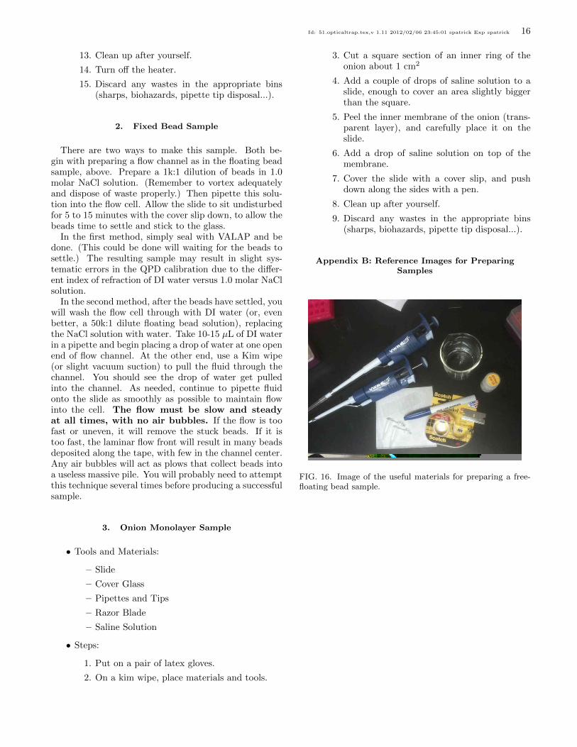
Appendix B: Reference Images for Preparing Samples

FIG. 16. Image of the useful materials for preparing a free-floating bead sample.

Id: 51.opticaltrap.tex,v 1.11 2012/02/06 23:45:01 spatrick Exp spatrick 17

FIG. 17. Image of the silica bead stock with relevant label FIG. 18. Image of the volume readout on the pipette. This information. is where to look when setting how many µL of solution you’d

like to draw for your sample.

FIG. 19. Image of Vortexer used to vibrate the solution.

Id: 51.opticaltrap.tex,v 1.11 2012/02/06 23:45:01 spatrick Exp spatrick 18

FIG. 20. Example slide with a double-sided tape channel and FIG. 23. Image of a beaker of heated VALAP used to seal coverslip. the ends of the channel.

FIG. 24. Cutting out a section of an onion, to extract a FIG. 21. Image detailing the use of a marker cap to press the

monolayer. coverslip to the double-sided tape and slide.

FIG. 25. Image of a finished onion slide; an onion monolayer FIG. 22. Injecting bead solution into the channel. in saline, between a slide and coverslip.

MIT OpenCourseWare https://ocw.mit.edu

8.13-14 Experimental Physics I & II "Junior Lab" Fall 2016 - Spring 2017

For information about citing these materials or our Terms of Use, visit: https://ocw.mit.edu/terms.