
ON THE RELATIONSHIP BETWEEN INNOVATION AND PERFORMANCE…bhhall/EINT/Loof_Heshmati.pdf · Lööf...
36
Lööf and Heshmati / On the Relationship Between Innovation and Performance: A Sensitivity Analysis 1 ON THE RELATIONSHIP BETWEEN INNOVATION AND PERFORMANCE: A SENSITIVITY ANALYSIS 1 HANS LÖÖF a and ALMAS HESHMATI b a Royal Institute of Technology, Industrial Economics and Management b The United Nations University, UNU/WIDER First Version May 2001, Revised October 2001, March 2002, December 2002. ABSTRACT We examine sensitivity of the estimated relationship between innovation and firm performance. In doing so, we rely on a knowledge production function approach and carry out comparisons in a number of ways. The sensitivity analysis is based on the comparison of: a basic econometric model estimated assuming different error structure and using the same data source, an identical model but different data sources, different classifications of firms performance, different classifications of innovation and the two main different subpopulations of the business sector. The analyses are performed in both level and growth rate dimensions. New findings are reported and previous results are confirmed as well. The study gives indications of what factors cause variations in the estimated effects of interest and the direction of changes. KEYWORDS: Knowledge capital, productivity, innovation, manufacturing, services, knowledge intensity, Community Innovation Survey. JEL Classification Numbers: C31, C24, L60, O31, O32 1 Hans Lööf acknowledges financial support from NUTEK and Almas Heshmati acknowledges financial support from the Service Research Forum (TjänsteForum). We thank participants at: The EU Commission Seminar on Innovation and Enterprise Creation: Statistics and Indicators, Nice 2000; The Workshop on Innovation, Technological Change and Growth in Knowledge-based and Service-intensive Economies, held at Stockholm on February 2001; The Conference on The Future of Innovations Studies, held in ECIS, Eindhoven on September 2001; seminars held at VINNOVA, NUTEK, Linköping University and CREST/INSEE; two anonymous referees, an Editor of the journal, Lars Bager-Sjögren, Paul Stoneman and Roger Svensson for their valuable comments and suggestions on earlier versions of this manuscript. Correspondence should be addressed to: Hans Lööf, Royal Institute of Technology, Industrial Economics and Management, SE 100 44 Stockholm, Sweden, E-mail: [email protected] and to Almas Heshmati, The United Nations University, UNU/WIDER, Katajanokanlaituri 6B, Fin-00160 Helsinki, Finland, E-mail: [email protected].
Transcript of ON THE RELATIONSHIP BETWEEN INNOVATION AND PERFORMANCE…bhhall/EINT/Loof_Heshmati.pdf · Lööf...

Lööf and Heshmati / On the Relationship Between Innovation and Performance: A Sensitivity Analysis
1
ON THE RELATIONSHIP BETWEEN INNOVATION AND PERFORMANCE: A SENSITIVITY ANALYSIS1
HANS LÖÖFa and ALMAS HESHMATIb
a Royal Institute of Technology, Industrial Economics and Management bThe United Nations University, UNU/WIDER
First Version May 2001, Revised October 2001, March 2002, December 2002.
ABSTRACT
We examine sensitivity of the estimated relationship between innovation and firm performance. In doing so, we rely on a knowledge production function approach and carry out comparisons in a number of ways. The sensitivity analysis is based on the comparison of: a basic econometric model estimated assuming different error structure and using the same data source, an identical model but different data sources, different classifications of firms performance, different classifications of innovation and the two main different subpopulations of the business sector. The analyses are performed in both level and growth rate dimensions. New findings are reported and previous results are confirmed as well. The study gives indications of what factors cause variations in the estimated effects of interest and the direction of changes.
KEYWORDS: Knowledge capital, productivity, innovation, manufacturing, services,
knowledge intensity, Community Innovation Survey. JEL Classification Numbers: C31, C24, L60, O31, O32
1 Hans Lööf acknowledges financial support from NUTEK and Almas Heshmati acknowledges financial support
from the Service Research Forum (TjänsteForum). We thank participants at: The EU Commission Seminar on Innovation and Enterprise Creation: Statistics and Indicators, Nice 2000; The Workshop on Innovation, Technological Change and Growth in Knowledge-based and Service-intensive Economies, held at Stockholm on February 2001; The Conference on The Future of Innovations Studies, held in ECIS, Eindhoven on September 2001; seminars held at VINNOVA, NUTEK, Linköping University and CREST/INSEE; two anonymous referees, an Editor of the journal, Lars Bager-Sjögren, Paul Stoneman and Roger Svensson for their valuable comments and suggestions on earlier versions of this manuscript.
Correspondence should be addressed to: Hans Lööf, Royal Institute of Technology, Industrial Economics and Management, SE 100 44 Stockholm, Sweden, E-mail: [email protected] and to Almas Heshmati, The United Nations University, UNU/WIDER, Katajanokanlaituri 6B, Fin-00160 Helsinki, Finland, E-mail: [email protected].
Lööf and Heshmati / On the Relationship Between Innovation and Performance: A Sensitivity Analysis
2
1. INTRODUCTION
New goods are at the heart of economic growth. The link between innovation and performance at various levels of aggregation has been the focus of attention in a number of studies in recent decades.2 The research in this area has resulted in interesting findings regarding expected effects, the data and methods used, and their benefits and limitations. The results, however, are different in many respects and the successive improvements in our understanding of economic behavior, data quality and econometric techniques calls for continued research.3
Summarizing the robust regularities which have emerged from a large number of studies at firm-level, Klette and Kortum (2002) present a list of stylized facts on the relationship between firm size, R&D effort, productivity and growth. Their list includes the following empirical findings. First, there is an approximately constant relationship between R&D and patents in the cross-sectional dimension but a negative relationship between R&D and patents in the longitudinal dimension.4 Second, there is a positive relationship between R&D activity and the level of productivity and across firms while the longitudinal relationship between firm-level differences in R&D and productivity growth is typically statistically insignificant.
In a survey of econometric studies of R&D and productivity at the firm level, Mairesse and Sassenou (1991) document widely varying estimates of the contribution of R&D to productivity. The variations are mainly observed across samples and model specifications and in relation to different estimation methods. The survey is based on 18 econometric studies at the firm level in the United States, France and Japan between 1969 and 1988. The authors suggest three important improvements to productivity studies. First, it is important that more research be carried out to improve the existing databases. In particular, emphasis is placed on the need to better account for quality aspects in the measurement of output, input prices and quantities. Second, it is essential to gain a better understanding of the diversity of the situations of individual firms and the evolution of these over time. The objective is to try to account for such diversity in terms of certain general statistics. The third improvement concerns a puzzling aspect in this area of research, reported by Klette and Kortum
2 For a selection of empirical studies or summary of empirical studies on the link between innovation
and productivity, see Griliches (1958, 1964, 1979, 1986, 1988, 1992, 1995) Mansfield (1961, 1962, 1965), Nelson (1962), Schmookler (1966), Pakes and Schankerman (1984), Griliches and Mairesse (1984), Kline and Rosenberg (1986), Cohen and Klepper (1996), Patel and Soete (1988), Mairesse (1990), Mairesse and Sassenou (1991), Lichtenberg and Siegel (1991), Pavitt (1993), Caballero and Jaffe (1993), Hall (1993), Hall and Mairesse (1995), Klette (1996), Klette and Griliches (1998), Crépon, Duguet and Mairesse (1998), Klomp and van Leeuwen (1999), and van Leeuwen and Klomp (2001), Lööf and Heshmati (2002), Klette and Kortum (2002).
3 The issue of econometric methods and data quality in productivity analysis is about as old as the discovery of the famous ‘residual’ in the 1950s. In their introduction to the volume containing papers presented at the NBER Conference on New Developments in Productivity Measurement and Analysis, Kendrick and Vacarra (1980) remind readers that one of the purposes of the 1958 NBER conference was to ‘suggest needed improvements in methods of estimation and basic data’.
4 It should be noted that this stylized fact differs from Cohen and Klepper’s (1996) stylized fact
number four, according to which the number of patents or innovations generated per dollar of R&D declines with firm size.

Lööf and Heshmati / On the Relationship Between Innovation and Performance: A Sensitivity Analysis
3
(2002), that estimates of R&D capital elasticity in the productivity equation obtained from time series data are much smaller and mostly insignificant compared to the elasticity obtained from cross-section data.
While the Mairesse and Sassenou paper contributes to an awareness of the presence of heterogeneity in results associated with a number of factors, Hall and Mairesse (1995) attempt to quantify the degree of heterogeneity in results. They further explore the causes of the generation of different estimates by using a single panel data set with relatively long time series data (17 years) but with varying specifications of the same model. The dynamics of investment in R&D are investigated, as is heterogeneity in investment behaviour. Their main finding is that more information on the history of the individual firms concerning R&D expenditures helps to improve the reliability of the estimates of R&D elasticity.
Based on the experience from previous sensitivity studies we have endeavoured in particular to acquire more detailed information on various key variables for individual firms and representative samples. Our goal was satisfactorily achieved by augmenting information from a large innovation survey with firm-level data on sales, value added, employment, human capital and financial information from register data obtained from Statistics Sweden. The data covers about 50% of all non-retail service and manufacturing firms in Sweden in 1998 with 20 or more employees.
In a promising innovation model recently developed by Crépon, Duguet and Mairesse (1998), a four-equation knowledge production function model was introduced which includes three relationships: the productivity equation relating innovation output to productivity, the knowledge production function relating investment in research to innovation output, and the research investment equation linking research to its determinants. An additional equation concerns investment decisions.
The Crépon, Duguet and Mairesse paper offers an attractive theoretical model and appropriate econometric methods for a better understanding of the processes containing what has been called a ‘black box’ by Rosenberg (1982 and 1994) and its relationship with innovation efforts and firm performance. Therefore, the regression results in our study are mostly based on an alternative version of the conceptual idea in this model. The modification was made given the nature of our cross-sectional data. Using versions of a multi-step procedure we will compare the estimated results of our main determinant factors with those reported in the literature.
The objective of this paper is thus to investigate the sensitivity of the estimated relationship between innovativeness and firm performance in a multidimensional framework. In doing so, we investigate the sensitivity of results with regards to different types of models, estimation methods, measures of firm performance, sub-populations of business sectors, different data sources, different specifications of innovation, level and growth rate dimensions. The results from various comparisons are tested for the importance of outliers.
The main contribution of this paper to the growing literature of the link between innovation and performance is the comprehensive multidimensional sensitivity analysis of the results and the extensive underlying data. The traditional analysis of the relationship between R&D and productivity is extended and developed by the use of firm-level data not previously available and state-of-the-art economic framework
Lööf and Heshmati / On the Relationship Between Innovation and Performance: A Sensitivity Analysis
4
which endogenize innovation in the explanation of heterogeneity in firm performance. New findings are reported and previous results are confirmed as well.
This study is one of the first attempts to estimate the causal effect of innovation investment on innovation output and the causal effect of innovation output on firm performance in both manufacturing and service industries using the same framework. An identical questionnaire, identical register data, the same estimation techniques and an identical specification of the model for both samples of firms are used for manufacturing firms and service firms. The performance is expressed in various measures and in both levels in growth rate terms. The innovations are explored with respect to their degree of novelty for both services and manufacturing firms.
The rest of this paper is organized as follows. In Section 2, the data is described. In Section 3, the model specification is outlined and estimation procedures are discussed. Empirical results from the main model are presented in Section 4, and results from the sensitivity analysis conducted in various dimensions are presented in Section 5. The final section concludes the discussion.
2. THE DATA, VARIABLES AND DEFINITIONS
The basic data used in this study was collected as an experimental enlargement of the second European Community Innovation Survey (CIS) conducted by Statistics Sweden.5 The data collection was carried out in 1999 and covers the period 1996 to 1998. In addition to the primary CIS information this survey also includes some other experimental information: product life cycle, rate of growth in the firm’s main market, the main customer of the firm and the most important factors for the attractiveness of the firm’s products and services.
In order to ensure that the data is suitable for our estimation purpose, we have imposed the following restrictions on the sample. First, we removed all observations for which the number of employees in 1998 was less than 20 and the amount of sales per employee was zero or missing. A second and necessary restriction applicable only to the growth analysis is the requirement that value added per employee, sales per employee, profit per employee and the number of employees must be positive in the first year observed (1996).
The information from the survey on innovation input, innovation output and exports as a share of total sales and various innovation indicators (factors hampering innovation activities, strategy on innovation, sources of knowledge for innovation and cooperation on innovation), has been supplemented with data on sales, value added, profit, physical capital and human capital from Statistics Sweden for firms in the innovation survey. Given the compulsory nature of the data collection, the register data suffers less from missing units of observation than the survey data. The quality of the data is improved through an intensive control process prior to making the data (in aggregate form) publicly available in various periodical publications.
We obtained 3,190 complete observations for 1998 and 2,899 complete observations for the period 1996-1998 (see Table 1). This data set covers more than 50% of all non-retail service and manufacturing firms in Sweden with 20 or more employees.
5 Sweden participated in the second Community Innovation Survey conducted in 1997.
Lööf and Heshmati / On the Relationship Between Innovation and Performance: A Sensitivity Analysis
5
2.1 Innovation and innovative firms
In order to distinguish firms by their innovative nature, we selected a sample consisting of only innovative firms. There is, however, no standard definition of an innovative firm or what distinguishes innovation from technical change. Schmookler (1966) suggests that when an enterprise produces a good or a service or uses a method or inputs that is new to it, it introduces technical changes. The enterprise that is first to make a given technical change is an innovator. Geroski, Machin and van Reenen (1993) stress the importance of not only innovation in itself, but also the learning process within the firm associated with innovation. Moreover, Hall (1994) noticed that the distinction between innovator and its followers – the imitator firms is often unclear. In their attempts to imitate, firms often do things differently (unintentionally or by design) from the way they were done by the first firm, and thus become innovators in their own way. The Oslo Manual (OECD, 1996), which set out the guidelines for the formulation and design of innovation surveys, includes technical change as well as imitation through questions on: products technologically new or significantly improved to the market, and products technologically new or significantly improved only to the firm.
Technical change is strongly attributed to production of goods, and the use of the same definition may fail to capture a majority of service innovations unless we redefine innovations one step further. In this study, we define innovations as goods and services that are both: (i) new or substantially improved to the market and (ii) new or substantially improved only to the firm. The effects of both these classifications of innovation can be analyzed jointly or separately.
We then define an innovative firm according to the following conditions: a firm is innovative if its innovation investment is positive, and if it also has positive innovative sales. Here by innovative sales, we refer to the sales revenue of a firm that is attributed to products (goods and services) introduced on the commercial market in the three most recent years. This condition resulted in a sample of 1,309 (41.0%) innovative firms, 903 of which are manufacturing firms, 363 service firms and the remaining 43 utility firms (see Table 2). However, the latter are not included in the analysis. The number in parentheses reflects the percentage of the total number of firms.
The non-innovative firms, according to our definition, consist of firms with neither positive innovation input nor positive innovation output during the period 1996-1998 (43.2%), firms with positive innovation input but no positive innovation output (12.5%), and firms with positive innovation output but no innovation input (3.2%). The non-innovative firms are retained in the total sample and are used in a selection equation for estimating a selection corrector variable which Heckman (1979) refers to as the inverse of Mill’s ratio.
Innovation sales according to our definition corresponds to 12% of all sales for the sample of service firms, 13% for the sample of manufacturing firms, 31% of sales for innovative service firms and 27% for innovative manufacturing firms. Hence, when all firms are considered, service firms and manufacturing firms are about equally innovative, but the average innovative service firm is somewhat more innovative than the corresponding manufacturing firms.
Lööf and Heshmati / On the Relationship Between Innovation and Performance: A Sensitivity Analysis
6
Innovation input is the total sum of expenditures on eight different categories of innovation engagements including: (i) R&D based products, services or process innovations within the firm, (ii) non-R&D based innovation activities (iii) purchase of services for innovation activities, (iv) purchase of machinery and equipment related to products, services and process innovations, (v) other non-machinery and equipment related innovation activities, (vi) industrial design or other preparations for production of new or improved products, (vii) education directly related to innovation activities, and (viii) introduction of innovations to the market.
2.2 A description of the statistics
Table 3 gives simple summary statistics for our key economic variables. The key variables include: innovation input, innovation output, sales, value added, profit before depreciation, profit after depreciation, sales margin defined as profit after depreciation as percentage of total sales, physical capital and human capital. All variables are measured in intensity terms, which means per employee except human capital, which is expressed as the percentage of engineers and the percentage of employees with a different university degree relative to total employment. The monetary variables are measured in SEK.
It is shown in Panel A and Panel B of Table 3 that the average firm in the innovation sample is larger (more employees), has a higher sales per employee, a higher value added per employee, and a larger proportion of employees with a university degree than the average non-innovative firm for services as well as for manufacturing. Non-innovative service firms are somewhat more profitable than the innovative service firms no matter whether profit per employee before or after depreciation or the sales margin is considered. The case is the opposite among manufacturing firms.
Table 4 shows summary statistics of growth rates for innovative and non- innovative firms between 1996 and 1998. Among the manufacturing firms (Panel B), it is clear that innovative firms are more dynamic than other firms in economic terms. Innovative firms have a higher growth rate of value added, sales and profit per employee. However, employment growth is slightly larger for non-innovative firms. The service sample is more ambiguous. While productivity increases fastest for the average innovative service firm, the non-innovative service firm has a larger rate of growth in sales and profit. Employment growth is approximately the same for both samples.
Finally, Tables 5 and 6 report the relationship between value added and sales, profit, innovation input, innovation output, human capital, physical capital and employment in both level and growth rate forms. In specification of the econometric models we account for a large number of production and innovation characteristics. Along with the usefulness of their inclusion they might cause serious problems of multicollinearity and difficulties in identifying their effects. Two simple ways of checking for the presence of multicollinearity are to look at the correlation coefficients among the explanatory variables and the R2 from regression of each explanatory variable on remaining explanatory variables. From Tables 5 and 6 we observed that the correlation coefficients vary in the interval –0.11 and 0.42. The R2 values are below 0.50. The low R2 values together with low correlation coefficients indicate that multicollinearity as not being a serious problem.

Lööf and Heshmati / On the Relationship Between Innovation and Performance: A Sensitivity Analysis
7
2.3 Treatment of extreme values
Given the restrictions imposed in Section 2, we have defined a ‘clean’ data set according to the following criteria. First, we censored any observation for which labour productivity and sales per employee were less than SEK 100,000 or more than SEK 10 million. This means that all observations with a productivity level less than SEK 100,000 per employee are replaced by observations equal to SEK 100,000, and observations more than SEK 10 million are replaced by SEK 10 million. Second, a similar censoring procedure was imposed on observations where the profit per employee before and after depreciation exceeded SEK 1 million. Third, in the profit specification of the model, we removed all observations for which profit per employee was zero or negative. The removal of such observations was justified by the logarithmic transformation of the data. There are 578 such observations, corresponding to 18.1% of the sample. Fourth, all observations for which the sales margin (profit after depreciation as a percentage of total sales) was less than -100% or more than 100% were also censored. Finally, we censored any observation for which the growth rate in value added, sales, and profit each expressed in per employee terms and employment for 1996 and 1998 was less than 75% contraction or more than 300% expansion. These censoring eliminate the influence of extreme observations and yet allows us to retain the observations in the estimation procedure.6
3. THE THEORETICAL FRAMEWORK
The theoretical framework for this study is a Cobb-Douglas production function explaining variation in firm output by a number of standard input variables and an additional R&D investment variable that can be represented schematically by the following equation: (1) εβββ +++= ∑ kxq kjj j0 where the lower-case letters denote log of variables expressed in per employee terms. The left-hand variable, q, is output produced, x is a J vector of standard input variables such as human capital, physical capital, material and energy, and k is R&D investment. The jβ is the elasticity of output with respect to a vector of inputs, kβ is the elasticity of output with respect to changes in R&D, and ε is the random error term.
A serious limitation of equation (1) is that it only measures the relationship between R&D input factors, k, and output, q. The neglected link is what Pakes and Griliches (1984) label it as ‘the knowledge production function’, i.e. production of commercially valuable knowledge or innovation output. They suggest an alternative
6 In analyzing the influence of outliers on the relationship between firm performance and innovation
we observed a relatively weak impact of outliers observations when value added and register data are considered. This finding is valid for both manufacturing and service firms. However, there is significant heterogeneity among censured and non-censured service firms when firm performance is measured as growth in sales.
Lööf and Heshmati / On the Relationship Between Innovation and Performance: A Sensitivity Analysis
8
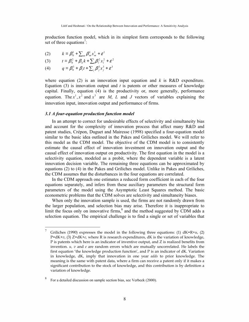
production function model, which in its simplest form corresponds to the following set of three equations7: (2) ∑ ++= m mm xk 1111
0 εββ (3) ∑ +++= l llk xkt 2222
0 εβββ (4) ∑ +++= j jjt xtq 3333
0 εβββ where equation (2) is an innovation input equation and k is R&D expenditure. Equation (3) is innovation output and t is patents or other measures of knowledge capital. Finally, equation (4) is the productivity or, more generally, performance equation. The 321 and, xxx are M, L and J vectors of variables explaining the innovation input, innovation output and performance of firms. 3.1 A four-equation production function model
In an attempt to correct for undesirable effects of selectivity and simultaneity bias and account for the complexity of innovation process that affect many R&D and patent studies, Crépon, Duguet and Mairesse (1998) specified a four-equation model similar to the basic idea outlined in the Pakes and Griliches model. We will refer to this model as the CDM model. The objective of the CDM model is to consistently estimate the causal effect of innovation investment on innovation output and the causal effect of innovation output on productivity. The first equation in the model is a selectivity equation, modeled as a probit, where the dependent variable is a latent innovation decision variable. The remaining three equations can be approximated by equations (2) to (4) in the Pakes and Griliches model. Unlike in Pakes and Griliches, the CDM assumes that the disturbances in the four equations are correlated.
In the CDM approach one estimates a reduced form coefficient in each of the four equations separately, and infers from these auxiliary parameters the structural form parameters of the model using the Asymptotic Least Squares method. The basic econometric problems that the CDM solves are selectivity and simultaneity biases.
When only the innovation sample is used, the firms are not randomly drawn from the larger population, and selection bias may arise. Therefore it is inappropriate to limit the focus only on innovative firms,8 and the method suggested by CDM adds a selection equation. The empirical challenge is to find a single or set of variables that
7 Griliches (1990) expresses the model in the following three equations: (1) dK=R+u, (2)
P=dK+v, (3) Z=dK+e, where R is research expenditures, dK is the variation of knowledge, P is patents which here is an indicator of inventive output, and Z is realized benefits from invention. u, v and e are random errors which are mutually uncorrelated. He labels the first equation ‘the knowledge production function’, and P is an indicator of dK. Variation in knowledge, dK, imply that innovation in one year adds to prior knowledge. The meaning is the same with patent data, where a firm can receive a patent only if it makes a significant contribution to the stock of knowledge, and this contribution is by definition a variation of knowledge.
8 For a detailed discussion on sample section bias, see Verbeek (2000).
Lööf and Heshmati / On the Relationship Between Innovation and Performance: A Sensitivity Analysis
9
strongly affects the probability of observation. In this case, the literature provides us with overwhelming evidence that the probability of engaging in R&D increases with firm’s size. Neglecting the selectivity problem by using standard regression techniques yield biased results.
In the production function model illustrated by equations (2) to (4), the innovation input k in equation (2) is an explanatory variable in the innovation output equation (3), and innovation output, t, is an explanatory variable in the productivity equation (4). Because of the endogeneity of these variables, we cannot assume that the explanatory variables and the disturbances are uncorrelated. As a result, an Ordinary Least Square regression applied to the Pakes and Griliches model will be biased and inconsistent. To overcome the problem of endogenous explanatory variables and derive consistent estimators, it is useful to consider a reduced form of the model, which is the method suggested by CDM. However, as an alternative to the CDM and its reduced form estimation method we consider an instrumental variables approach and impose different assumptions concerning the disturbances.
3.2 A structural multi-step approach
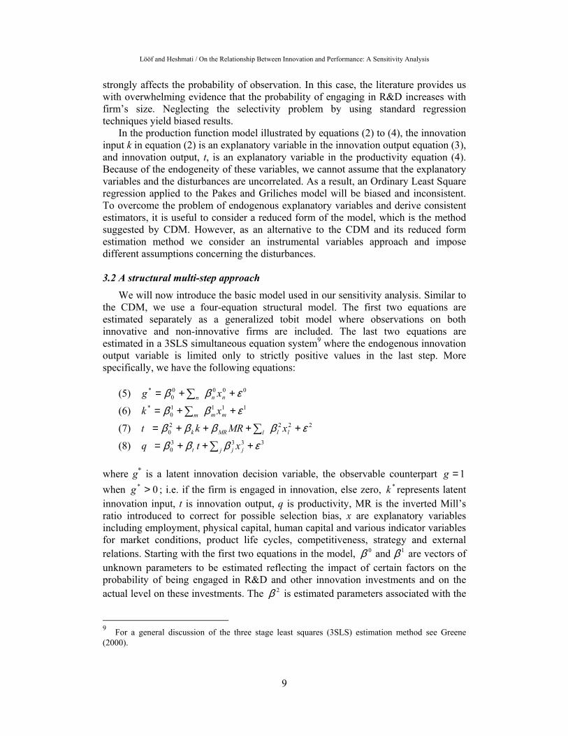
We will now introduce the basic model used in our sensitivity analysis. Similar to the CDM, we use a four-equation structural model. The first two equations are estimated separately as a generalized tobit model where observations on both innovative and non-innovative firms are included. The last two equations are estimated in a 3SLS simultaneous equation system9 where the endogenous innovation output variable is limited only to strictly positive values in the last step. More specifically, we have the following equations:
(5) 0000
0* εββ ++= ∑ nnn xg
(6) 11110
* εββ ++= ∑ mmm xk
(7) 22220 εββββ ++++= ∑ lllMRk xMRkt
(8) 33330 εβββ +++= ∑ j jjt xtq
where g* is a latent innovation decision variable, the observable counterpart 1=g when 0* >g ; i.e. if the firm is engaged in innovation, else zero, *k represents latent innovation input, t is innovation output, q is productivity, MR is the inverted Mill’s ratio introduced to correct for possible selection bias, x are explanatory variables including employment, physical capital, human capital and various indicator variables for market conditions, product life cycles, competitiveness, strategy and external relations. Starting with the first two equations in the model, 10 and ββ are vectors of unknown parameters to be estimated reflecting the impact of certain factors on the probability of being engaged in R&D and other innovation investments and on the actual level on these investments. The 2β is estimated parameters associated with the
9 For a general discussion of the three stage least squares (3SLS) estimation method see Greene (2000).
Lööf and Heshmati / On the Relationship Between Innovation and Performance: A Sensitivity Analysis
10
level of innovation output while 3β is associated with both the level and growth rates of productivity. In the growth version of the model, a lagged production variable appears as initial value of productivity in equation (8).
Equations 5 and 6 are estimated jointly in a generalized tobit model. The 10 and εε are random error terms with mean zero, constant variances and not
correlated with explanatory variables. However, the two error terms are correlated with each other. In the tobit equation 6, k represents the level of innovation investment. From the generalized tobit model estimates of k and MR variables are obtained and are used as explanatory variables in equation 7. Equations 7 and 8 are estimated based on data with positive innovation input and outputs. Since there is no direct link between innovation input and productivity the inverted Mill’s ratio variable is not included in equation 8. However, it has an impact on productivity through predicted innovation output which is an explanatory variables in productivity equation.
One possible problem with the production function approach is that explanatory variables are often determined jointly with the dependent variable, i.e. they are not exogenously given.10 The last step of the model highlights this simultaneity problem. The innovation input, k, is endogenous in the innovation output equation (7), and innovation output, t, is endogenous in the productivity equation (8). In order to derive a consistent estimator, our model accounts for simultaneity bias by relying on the instrumental variable approach. The instruments consist of variables not correlated with the model error term but correlated with the endogenous variable.
The explicit use of instrumental variables is one important difference between our model and the CDM. The second main difference is that by estimating equations (7) and (8) separately from (5) and (6), we allow for limited correlation between the error terms of the equations in the model. We believe that, by splitting the model into two parts, we avoid allowing for full correlation structure of the error terms and thereby a tractable estimation procedure and easier interpretable results. We are aware of the necessity of modeling correlation among the residuals within the two parts separately and also between the two parts. It is important to be noted that we still account for some degree of correlation by linking the two parts using the Mill’s ratio variable. Our approach is thus an intermediate approach compared to the Pakes and Griliches (1984) model which neglects any form of correlation and the Crépon, Duguet and Mairesse (1998) approach allowing for full correlation between the four residuals. The variance covariance matrix in our model is a block diagonal where the elements in the off-block-diagonal consist of a scalar linking equations (6) and (7).
The CDM with its full correlation assumption implies that forces that have an impact on the estimated probability of being engaged in R&D also influences the estimated elasticity of productivity and vice versa. This assumption is supported by studies on R&D and productivity carried out in the past few decades. However, capturing this dynamic relationship, which goes in both directions, between R&D and productivity, requires the time aspect to be taken into account. Ideally, one would study how R&D investment in year τ−t influences productivity in year t and how
10 For a detailed discussion on the identification related to the estimation of production functions, see
Griliches and Mairesse (1997).

Lööf and Heshmati / On the Relationship Between Innovation and Performance: A Sensitivity Analysis
11
productivity in year t influences the R&D investments in year τ+t . With long time series and detailed lag structure, it may be possible to analyze a recursive equation system with current output depending on past R&D, and with past R&D depending on past rather than current output.
In the cross-sectional data used in this paper, we can only observe the firms’ R&D or innovation investment for a single year. We must therefore assume that the level of investments in year t can be used as an acceptable proxy for permanent R&D, i.e. the firms do not experience major fluctuations in their R&D investments behaviour. The literature shows that R&D expenditures are highly correlated from one year to another (Griliches, 1998). An additional argument in support of our version of the knowledge production function is the fact that we have only information about innovation output at end of the second period. The use of a dynamic approach as in the CDM model would require that the innovation output to be time variant as well.
3.3 Model specifications
The basic model used in this paper will be applied separately to a sample containing only service firms and a sample containing only manufacturing firms. The specification of the model is identical for both samples. We will now present the specifications of the four equations of the model.
The x0 variables in the selection equation consist of employment, physical capital per employee, engineers (those graduated from a technical university and those with two years of post secondary education) and administrators (holding a non-engineering degree), 7 dummy variables for the firm’s main customers and 9 dummy variables representing factors perceived as strongly important for the firm’s products. Size and physical capital are measured in logarithmic terms, and human capital is measured as the percentage of engineers and administrators relative to total employment. Administrators are defined as all other non-engineer employees with a university degree. Five industry dummies are included in the service sample and 23 industry dummies in the manufacturing sample. The reference group includes the remaining labour force, consisting of blue-collar and white-collar workers with lower education.
The determinants of innovation input labeled as the 1x vector consist of the firm’s main customer (7), strongly important cooperation partners (8), strongly important innovation strategies (7), obstacles to innovation (9), product life cycle (5), and growth rate in the firm’s main market (4). Dummy variables for process innovation, organizational innovations and industry dummies are also included. Three quantitative variables are included in the equation: employment, physical capital and exports. The number in parentheses indicates the number of dummies representing different alternatives containing the respective characteristic variable. The absence of numbers after a variable indicates a single column variable.
The determinants of innovation output, the 2x vector, consist of employment, physical capital, predicted value of innovation input, inverted Mill’s ratio, predicted value of firm performance (feedback effect), strongly important sources of information or innovation (13), strongly important cooperation partners on innovation (7), and growth rate in the firm’s main market (4)11. Two additional indicator
11 One might suspect that the export market and market growth variables in the innovation input equation (6) be correlated. However, a simple correlation test

Lööf and Heshmati / On the Relationship Between Innovation and Performance: A Sensitivity Analysis
12
variables are included: products new to market mainly developed in cooperation with others and products new to the firm mainly developed without any cooperation with external partners.
Finally, the 3x vector contains information on employment, physical capital, predicted innovation output, lagged value of firm performance (only the growth version of the model), human capital variables, process innovation, innovation organization, three composite dummy variables for different innovation strategies, engineers and administrators as defined earlier, and industrial sector dummies.
The dependent variables include log innovation input per employee, k, in equation (6) log innovation sales per employee, t, in equation (7); in the last performance equation (8), q, is defined in several alternative ways. The alternative definitions include: value added per employee, sales per employee, profit before and after depreciation per employee - all in logarithmic forms - and sales margin when the level dimension of the model is considered. The performance measures in the growth rate version are growth of labour productivity, growth of sales, growth of profit per employee and growth of employment.
The information set in the CDM and those in our model differ in many important ways. Although the basic idea is estimation of a knowledge production function and establishment of causal relationship between the variables of interest, the lack of full overlapping of the two data sets used in the current and CDM studies do not allow application of identical model specification.
4. EMPIRICAL RESULTS
In order to investigate the sensitivity of the estimation results, we perform a number of comparisons. The first sensitivity analysis is based on results from a sample with manufacturing firms and different combination of accountancy for selectivity and simultaneity. One of the alternative models ignores both selectivity and simultaneity problems (Model 1), one only accounts for simultaneity bias (Model 3) and the last one corrects only for selection bias (Model 4). Model 4 ignores simultaneity of innovation output and productivity equations. However, in a multi-step procedure it accounts for endogeneity of innovation input, innovation output and productivity. Analysis of the results in the following sections are based on those obtained using the basic model (Model 2) which accounts for both sources of bias.
In the second sensitivity analysis, we compare the sample of manufacturing firms with the sample of service firms. Estimates that are statistically significant for both categories of firms are presented in the level dimension. In the third sensitivity analysis we compare results based on different measures of firms’ performance in level as well as in growth rate dimensions and compare both categories of firms. The fourth test is a comparison of the impact of innovations new to or significantly improved for the market versus the impact of innovations new to or significantly improved for only the firm. We compare the two types of innovations for both samples in a level and growth dimensions. Finally, we compare the elasticity of sales per employee when different data sources are considered. The impact of different
indicates that the correlation between export intensity per employee and the growth rate in a firm’s main market is rather weak, reducing the relevance of such problems.

Lööf and Heshmati / On the Relationship Between Innovation and Performance: A Sensitivity Analysis
13
treatments of extreme values of the dependent variable on the results is also examined. 4.1 Different estimation procedures
The results of estimating four different models for the manufacturing sample in log levels and in growth rates forms are given in Table 7. To conserve space, we only report the elasticity of log value added per employee and the growth rate of value added per employee, each with respect to log innovation sales per employee.
The estimation procedures are as follows. Model 1 corresponds to the standard Ordinary Least Squares method applied to equations (1) or (8). The model ignores simultaneity bias as well as selectivity bias. Only innovation firms data are included in the estimation.
Model 2 is the basic model presented in equations (5)-(8). This is a structural two-step regression model. The first step consists of a generalized tobit model applied on the total sample of innovative and non-innovative firms, and the second step consists of a simultaneous system including only observations with strict positive values on the innovation input and output variables. The inverted Mill’s ratio computed from the estimated parameters of the selection part of the generalized tobit model together with instruments for the endogenous innovation input variables are introduced in the simultaneous equation system. This model accounts for both selectivity and simultaneity issues.
Model 3 is similar to Model 2 but without the inverted Mill’s ratio. The model therefore ignores selectivity but takes simultaneity into account.
Model 4 is a five-step least square model. The first two steps are equivalent of the generalized tobit model in Model 2 and Model 3, where all observations are included disregards of innovative nature of the firms. The third step is an OLS regression for the total sample with productivity as the dependent variable. The fourth step consists of an innovation output equation using OLS for only the innovation sample. Predicted productivity from step 3 and the inverted Mill’s ratio from the generalized tobit model are included among the explanatory variables in the innovation output equation. The last step is an additional productivity equation, but now with the predicted innovation output from equation 4 as a control variable. The explanatory variables in the innovation output and productivity equations are more or less the same as in the basic model. This model accounts for selectivity bias through the inverted Mill’s ratio; it accounts for endogeneity of explanatory variables, however, the simultaneity bias has not been properly accounted for.
Panel 7.A reports the innovation output elasticities in the log level dimension. Taking the OLS estimate in Model 1 as a benchmark value. It is 0.054 and highly significant. However, it can be expected that the model suffers from a serious methodological problem. The sample used in the regression is not random. Furthermore, the presence of endogenous explanatory variables in the relation is also another problem.
Before discussing the results from the multistep models we will briefly show some evidence from the literature on the relationship between innovation and performance. Based on a version of the standard model (equation 1), Griliches (1984) found cross-section estimates of the size 0.07 for 883 US manufacturing firms. Mairesse and Cuneo (1985) estimated the elasticity of productivity with respect to
Lööf and Heshmati / On the Relationship Between Innovation and Performance: A Sensitivity Analysis
14
R&D to be 0.10 for 296 scientific firms in France. The standard errors were in the interval 0.01-0.02 in both cases.
Model 2 is our basic model which account for the selectivity and simultaneity problems by using the inverse Mill’s ratio and instruments in the simultaneous equation system. This results in a significantly larger estimate of 0.121 for the innovation output. When we exclude the inverted Mill’s ratio variable from the basic model, we find results from Model 3 to be identical to those of Model 2, suggesting that the simultaneity problem is more severe than the selectivity problem. When we account for selectivity in Model 4 and ignore simultaneity bias, the innovation output estimate is higher, 0.166.
We observe negative and weakly significant selection bias in Model 2, but insignificant selection bias in Model 4. Given the lack of highly significant selection effects, the minor differences between the key elasticties among the two models reported in Table 7 can be attributed to simultaneity bias. In a smaller data set from an earlier period (1994 to 1996) we found evidence of selection bias for manufacturing firms but not for another Swedish data set consisting of plant level manufacturing (see Lööf and Heshmati, 2002). The current study is based on a much larger data set observed for a later period of 1996 to 1998. However, we cannot exclude the possibility that some variables in Model 4 are uncorrelated with the error terms, but correlated with endogenous variables serving as instruments. This is reflected in the significant differences between Model 1 and Model 3 associated with simultaneity issue.
Turning to Panel 7.B and the four various growth rate estimates, we find that the simple OLS model (Model 1) reports a weak impact of innovation output on productivity growth. The estimated effect is 0.024 and statistically significant at the 1% level of significance. This result from the standard model can partially be compared with an elasticity of productivity with respect to research of the size 0.12 (0.02) for time-series of cross-section of a sample of 652 manufacturing firms in the US for the period 1966-77. Mairesse and Cuneo reported 0.11 (0.04) for 390 manufacturing firms in France for 1974-79. It is to be noted that by partial comparability of results we mean that the results reported by Mairesse and Cuneo are based on time series of cross sections (panel data) while our results are based on a cross section sample where the productivity variable is expressed in growth rate form.
The estimate nearly triples to 0.070 when the basic model (Model 2) is used and it is significant. Using Model 3, which ignores selectivity bias, gives about the same estimate as of Model 2. However, the standard errors are larger and the estimate is significant at the 5% level of significance. Finally, the multi-step procedure model produces a point estimate of 0.073, and it is only weakly significant.
Summarizing the findings presented in Table 7 shows that the simple OLS model gives downward biased elasticities due to its ignorance of selectivity and simultaneity biases and less appropriate for analyzing the relationship between innovation and productivity. The basic model produces highly significant estimates in log level and in the growth rate dimensions. The size of estimates is within the range of what has been found in previous literature, although we use a broader definition of innovation output compared to the traditional definition, which focuses on technology. Model 3, which only takes simultaneity bias into account and ignores selectivity bias, produces similar innovation output effects and larger standard errors particularly in the growth rate
Lööf and Heshmati / On the Relationship Between Innovation and Performance: A Sensitivity Analysis
15
dimension compared to the basic model. The results from Model 4, which accounts for selectivity but at least partly it ignores simultaneity bias, differ from the results produced by the basic Model 2. It produces an upward biased estimate. A tentative conclusion is that the issues of simultaneity are found to be of great importance.
The CDM study reported presence of significant selection bias. In our model the coefficient of Mill’s ratio is about -0.30 in both level and growth dimensions, but only weakly significant at the 10% level of significance. The differences in degree of significance in comparison with the CDM case might be due to a combined result of the different assumptions regarding the correlation among the equation residuals and in the way the models are specified.
4.2 A Comparison between service and manufacturing firms
Our next sensitivity analysis concerns the results with respect to different samples of firms. An identical questionnaire, identical register data, the same econometric framework and an identical model specification are used for both manufacturing firms and service firms. The results of estimating the basic model in the level form of log value added per employee as performance are given in Table 8. Table 9 extends the comparison between the two industries by reporting results for different performance measures as well as for both the level and growth rate dimensions.
The likelihood of performing innovation rises with firm size for both types of firms (see Panel 8.A). The size of the estimates is about the same for both samples. The physical capital and the share of engineers correlate significantly with the dependent variable for manufacturing but not for services. The other human capital variable, administrators, is insignificant in both cases.
Among the nine dummy variables indicating factors that are perceived to be strongly important for the competitiveness of a firm’s products, ‘high quality’ is highly significant in both samples, ‘high delivery security’ only for service firms and ‘trademark’ only for manufacturing firms.
When the innovation input equation in Panel 8.B is considered, firm size enters the regression significantly and is negative for both manufacturing and services. Innovation input is positively correlated with physical capital per employee only for manufacturing firms and to our surprise with export sales per employee only for services.
Problems with external cooperation on innovation are positively associated with the level of innovation investments for service firms in particular and significant at the 1% level. This is true for manufacturing but only significantly at the 10% level. The unexpected sign of this estimate can be interpreted in two different ways: (a) the firms increase their internal innovation activities because of difficulties in cooperating on innovation and sharing expenses, or (b) firms with a high level of innovation investments per employee have a greater likelihood of participating in innovation collaboration, and this activity is by its very nature complex and a vast number of problems must continuously be solved.12 We believe that the sign of the estimate 12 An interpretation close to the (b) interpretation would simply be that this variable measures R&D
cooperation itself. If this is the case following the theoretical literature on R&D cooperation we should expect higher investments in innovation. The seminal paper on this topic is by D’Aspremont and Jacquemin, (1988). The authors show that, when spillovers are strong, firms that cooperate in R&D invest more in innovation than firms that do not (if they remain competitors in the same

Lööf and Heshmati / On the Relationship Between Innovation and Performance: A Sensitivity Analysis
16
reflects the latter interpretation. Among service firms, the lack of appropriate technology correlates negatively with innovation efforts.
Panel 8.C shows that the level of innovation sales per employee is positively correlated with the size of innovations investment per employee for both manufacturing and service firms. Interestingly, the magnitude of the estimate, the standard errors and hence the degree of significance are very similar. This finding is not in agreement with Klette and Kortum (2002), who report a constant relationship between R&D and innovations output measured as patents. However, using the CDM model, Crépon, Duguet and Mairesse (1998)13 found that the elasticity of innovation output with respect to R&D capital per employee is in the region of 0.3-0.4, compared to 0.5-0.6 in our study.14
Innovation output is weakly positively correlated with firm size in the case of services. No such correlation was found for the manufacturing firms. This finding can be compared with Cohen and Klepper (1996), who report a negative relationship between the number of innovations generated per dollar of R&D and firm size. Innovation output increases with the growth rate in the firm’s main market in both samples. Only for the average service firm we find a significant correlation between professional conferences, scientific journals and innovation output.
The innovation output equations contains dummy variables for products new to the market mainly developed internally within the firm and products new to the firm mainly developed without cooperation with others. The latter is expected to indicate whether the firm has enough internal competency necessary for incremental innovation while the former indicates whether the innovative firm typically is part of a network of firms developing products new to the market. Unlike our a priori expectations, Panel 8.C shows that information technology is the only important source of knowledge for innovation that correlates significantly with innovation output. Professional conferences and suppliers contributes with knowledge to service innovations. Considering products new only to the firm and mainly developed by internal knowledge, we find that this variable is highly significant for both types of firm.
The level of labour productivity increases significantly and positively with the intensity of innovation sales for both samples of firms. It is interesting to note that the size of the estimates does not differ much between service firms and manufacturing
product market). Many other papers have been written since on this topic and find the same result.
13 The four-equation CDM model applied by Crépon, Duguet and Mairesse to a sample of 4,164
manufacturing in France gave estimates of the following sizes. The coefficient of the log number of employees in the probit equation (the probability of doing R&D) is 0.4. The coefficient of log number of employees in the tobit equation (2) where research effort per employee is the dependent variable is about 0.0. The coefficients of log R&D capital per employee and log employment was about 0.3-0.4 and 0.0, respectively, in the innovation output equation. When the logarithm of value added per employee is the dependent variable, the coefficient of log innovation output per employee is 0.1, and that of log physical capital per employee is 0.2. The corresponding figure for engineers as a percentage of total employment is 1.7, for administrators as a percentage of total employment, 1.8 and for the log employment about zero.
14 Crépon, Duguet and Mairesse (1998) used the stock of R&D while we have used a flow measure of
total innovation input.
Lööf and Heshmati / On the Relationship Between Innovation and Performance: A Sensitivity Analysis
17
firms. It is 0.09 for service firms and 0.12 for manufacturing firms. However only the former is significant at the 1% level.
The size of our estimates can be compared with 0.07-0.10 for two different versions of the CDM model reported by Crépon, Duguet and Mairesse. This gives some evidence that our broader measure of innovation, aimed at capturing innovations in services, might be a reasonable definition.
The share of university graduated employees is found to be strongly correlated with the productivity of manufacturing firms. The coefficient is 1.3 for administrators and 1.0 for engineers. Considering services, the estimate is 0.4 for engineers and 0.5 for administrators. The later significant only at the 5% level. Crépon, Duguet and Mairesse found even larger skill estimates for manufacturing in France.
Value added per employee increases with capital per employee for both sectors. The size of the estimate is 0.14 for manufacturing and 0.05 for services. In the literature, the size of the capital elasticity is found to be in the interval 0.2-0.3 for manufacturing firms.
The estimated elasticity of productivity with respect to innovation output increases by about 50% when we do not control for physical capital. The lack of a control for skill increases the elasticity by about 25%.
Our last finding concerns the strategy on innovations. An explicitly offensive innovation strategy correlates positively with productivity for the innovative service and manufacturing firms.
The overall picture in comparing manufacturing firms and service firms is one of striking homogeneity regarding the estimated relationship between innovation input and output and between innovation output and the level of productivity. This finding has not been well documented in previous studies. One reason is that innovation data from service firms is still rare. In fact, the innovation survey used was designed by the authors in collaboration with the Statistics Sweden as an experimental enlargement of the CIS survey. In the original CIS survey information is not acquired about innovation output among services. However, this was changed in the third round of the CIS surveys launched in Europe in 2001.
4.3 Different performance measures
Our next sensitivity analysis concerns the use of different measures of firm performance and samples of firms. The results of estimating the basic model in log levels and in growth rates are given in Table 9. To conserve space, we only report the elasticity of firm performance with respect to innovation output.
Panels 9.A and 9.B report the innovation output elasticity for five different performance measures in the level dimension for services and manufacturing. The first four measures are the logarithm of value added per employee, sales per employee, profit before depreciation per employee and profit after depreciation per employee. Because the logarithmic values only contain strictly positive values, about 10% of the observations with negative profit before depreciation and 20% of the observations after depreciation are excluded from the analysis. As a consequence, the estimated impact of innovation on profit will be overestimated, particularly in the later case. The last measure is sales margin, defined as profit after depreciation as a proportion of total sales. Since all observations are included here, it is our prime

Lööf and Heshmati / On the Relationship Between Innovation and Performance: A Sensitivity Analysis
18
measure in analyzing the relationship between innovation and profit in the level regressions.
Panels 9.C and 9.D report the innovation output elasticity in the growth rate cases. The performance measures are annual growth of value added per employee, sales per employee, profit before depreciation and, profit after depreciation and employment.
The results show that the elasticity of value added per employee in level and growth rate dimensions makes little differences between manufacturing and services (see Panels 9.A-9.D). Although these estimated impact of innovation on productivity are subject to a variety of econometrics and other reservations, there is a striking similarity between samples of firms, which are not well documented in the literature. Contrary to value added, the employment increases with innovation output only for service firms. The estimate is 0.12 and highly significant.
The next finding is that the elasticity of sales per employee is considerably larger than the elasticity of value added per employee in both services and manufacturing samples. We can confirm previous findings which indicate that sales is a crude proxy for value added. Our results suggest that researchers must be careful in interpretation of sales estimates when services are considered.
Panels A and B shows the magnitude of bias due to eliminating observations with negative profit. Since we cannot transform negative values to logarithmic terms 23% of the innovative firms in the service sample and 18% of the innovative firms in the manufacturing sample are excluded. The elasticity of profit after depreciation with respect to innovation output is 0.36 (standard error 0.14) for service firms and 0.45 (0.12) for manufacturing firms. A replacement of profit by using a non-profit measure of productivity but on same observations gives highly significant estimates for both samples of firm. The magnitude is 0.30 (0.04) for service firms and 0.29 (0.04) for service firms.
In the growth rate dimension and when using the samples with only positive profit, we find a positive correlation between the rate of growth of profitability and innovation output only for service firms.
Considering the alternative profit measure sales margin, which is observed for all firms, Panel 9.B shows that a manufacturing firm’s sales margin increases with innovation output but it is significant only at the 10% level of significance. Panel 9.A reports no significant estimates at all for service firms. Finally we find that sales growth increases with the level of innovation output but only for manufacturing.
To conclude, when different performance measures are considered, sales is a less appropriate proxy of value added when the relationship between innovation and performances is analyzed. Productivity increases with innovation output for services as well as for manufacturing, and in both the level and in the growth rate dimensions. The reported strong association between profitability and innovation is overestimated due to the presence of selection bias. Employment increases with innovation output only for services while no correlation between innovation intensity and profit growth can be established for neither of the categories of firms.
4.4 Different types of innovation
Innovations can be distinguished on the basis of their degree of novelty. Here we explore the impact of innovations new to the market or innovations new only to the firm on firm’s performance. Barlet et al. (2000) suggest the presence of two distinct

Lööf and Heshmati / On the Relationship Between Innovation and Performance: A Sensitivity Analysis
19
and opposite effects. The first effect, labeled inertia, is interpreted as the greater the novelty, the greater is the risk associated with the introduction of innovations. New products are only gradually accepted by the market. If this effect dominates, we would a priori expect a weaker relationship between innovations new to the market and firm performance than a case where innovations are only new to the firm. However, if the second effect, labeled efficiency effect, dominates, i.e. if the novelty is a response to market demands and is valued by the market, then products new to the market are the most productive or profitable innovations. Here efficiency can be interpreted as value effect.
Panels 10.A and 10.B present the elasticities of five different measures of firm performance with respect to innovation output in the level regressions, and Panels 10.C and 10.D show the corresponding elasticities for the growth rate dimensions. The different performance measures are identical to those in Table 9 presented previously.
Panels 10.A1 and 10.A2 compare the innovation output estimates with respect to the degree of novelty for services, and 10.B1 and 10.B2 for manufacturing firms. It is shown that the elasticity of performance in level form with respect to innovation output is typically largest for innovations new only to the firm for both services and manufacturing when sales, value added and sales margin are considered, thus supporting the inertia hypothesis. Note, however, that the number of observations with innovations new to the market is larger than the number of observations with innovations new to the firm.
A look at the logarithms of profit per employee reveals a more ambiguous pattern. Among services, the elasticities are larger for innovations new to the firm while there are no significant difference for manufacturing firms. We will again remind the reader that the measures of log level of profit are limited to only observations with positive values of profit. This result should be interpreted with caution.
Panels 10.C1 and 10.C2 present growth rate estimates for services. Panels 10.D1 and 10.D2 give the corresponding estimates for manufacturing. The interesting finding here is that the productivity growth increases with innovations new to the market among manufacturing firms but not with innovation new to the firm. Duguet (2002), finds exactly the same result for the French manufacturing, using the same kind of data set as in CDM. For services both categories of innovations are positively related to productivity growth. The results presented in Table 9, showed that a positive and significant relationship between innovation and employment growth could only be found for services. Panels 10.C1 and 10.C2 reveals that this relationship is neutral in terms of the degree of novelty of the innovations.
The main empirical findings presented in Table 10 can be summarized as follows. There is a closer relationship between innovation output and the level of value added per employee, the level of sales per employee and sales margin when innovations new to the firm are considered. On the contrary, the growth rate of productivity increases only with innovations new to the market in manufacturing. The positive relationship between innovation and employment growth and innovation and productivity growth for service firms is independent of the degree of novelty of the innovations.

Lööf and Heshmati / On the Relationship Between Innovation and Performance: A Sensitivity Analysis
20
4.5 Censoring and different data sources
Table 11 presents estimation results that are based on an identical model specification but are estimated using different sources of data, namely register data and survey data. In addition we also explore the importance of censoring the data. Only estimates for sales per employee in level and growth rate dimensions. The survey data does not contain any value added measures reported here.
The first row of Table 11 provides estimated elasticities based on register data where the outlier observations have been censored according to the censoring conditions mentioned previously. The results are compared with the regression results reported on the second row where the outlier observations are retained. The third and fourth rows provide the corresponding regression results but based on survey data. In the level dimension, the register data has about 10% more observations than the survey data, and the difference in the number of observations increases to about 20% when the growth rate dimension is considered.
Starting by comparing censored register data versus censored survey data the first finding is that the estimates in the level dimension are about the same size for manufacturing firms but 50% larger for service firms when register data on sales is used. The second finding is that the growth rate estimates are highly significant for manufacturing and services only when register is used.
Comparing censored and non-censored data Table 11 reports that the differences are negligible in the level dimension irrespective of the data source. In the growth rate dimension we have already found that register data is superior to the survey data. To this we can add that non-censored register data produces significantly a different estimate for service firms compared to the censored case for service firms. The elasticity of sales growth with respect to innovation output is 0.12 and significant at the 5% level. It declined to 0.05 and insignificant when three extreme observations are included.
The conclusion regarding different sources of data using an identical model is that register data is preferable to survey data if both are available. The quality of survey data is particularly questionable when growth regressions are considered. The only case where the influence of outliers is clearly identified is in the growth rate dimension, and the elasticity of sales per employee with respect to innovation output is estimated. It is possible that some data have been misreported, but is also possible that some firms have sold parts of their activities or have acquired activities of other firms, which could explain some of the unrealistic growth rates.
5. CONCLUSIONS
This study was aimed at investigating the sensitivity of the estimated relationship between innovativeness and firm performance. We compared the sensitivity of results with regards to different types of models, estimation methods, measures of firm performance, classification of firms, type of innovations and data sources. The analyses were performed in both level and growth dimensions of firm performance, and investigated the influence of outlier observations on the results.
The data set used contains detailed information on various key characteristics of firms. This includes information related to R&D, other innovation inputs, various innovation indicators, the outcome of the innovation processes and other variables
Lööf and Heshmati / On the Relationship Between Innovation and Performance: A Sensitivity Analysis
21
from the survey at the individual firm level augmented with the register data. The combined data is comprehensive and covers about 50% of all non-retail service and manufacturing firms with 20 or more employees in Sweden in 1998.
We find that the simple least squares method estimation of the model produces downward biased elasticities due to the ignorance of selectivity and simultaneity problems. We find it inappropriate for analyzing the relationship between innovation and productivity. Estimation of the basic model produces significant estimates in both log level and growth rate forms. The size of the estimate is within the range of what has been found in previous literature. An alternative procedure, in which only simultaneity bias is taken into account but selectivity bias is ignored, produces similar innovation output effects compared to the basic model. The results from a model which accounts for selectivity but partly ignores simultaneity bias, differs from the results produced by basic model procedure. It produces an upward biased estimate. A tentative conclusion is that the issues of simultaneity are found to be of great importance.
In a comparison of manufacturing firms and service firms, there is striking homogeneity regarding the estimated relationship between innovation and productivity that previously has not been well documented in the literature. This similarity is observed in both level and growth rate dimensions. Our conclusion supports the view that services and goods are not much different and productivity or performance analysis raises similar difficulties for both sectors.
A consideration of different performance measures shows that sales is a less appropriate proxy for value added when the relationship between innovation and performances is analyzed. Employment increases with innovation output only for services while no strong correlation can be established between innovation intensity and growth in profit for neither categories of firm. There is a close association between the level of profit and innovation for services as well as for manufacturing firms. However, due to the exclusion of observations with negative profit the impact of innovation might be overestimated.
We find a closer relationship between innovation output and the level of value added per employee, the level of sales per employee and sales margin for innovations new to the firms compared to cases where innovations are new to the market. On the contrary, the growth rate of productivity increases only with innovations new to the market when manufacturing firms are considered. The positive relationship between innovation and employment growth and innovation and productivity growth for service firms is independent of the degree of novelty of the innovations.
Our conclusion regarding the use of different sources of data while using an identical model specification is that register data is preferable to survey data when both data sources are available. The survey data is particularly unreliable when growth regressions are considered. The only case where the influence of outliers is most influential is in the growth rate dimension and when the elasticity of sales per employee with respect to innovation output is estimated.
Lööf and Heshmati / On the Relationship Between Innovation and Performance: A Sensitivity Analysis
22
REFERENCES
Barlet C., E. Duguet, D. Encaoua and J. Pradel, 2000, The Commercial Success of Innovations: An Econometric Analysis at the Firm Level in French Manufacturing, in: D. Encaoua et al. (eds), The Economics and Econometrics of Innovation, Boston: Kluwer Academic Publishers, pp. 435-456.
Caballero R. J. and A. B. Jaffe, 1993, How High are the Giants Shoulders? In O. J. Blanchard and S. Fisher (eds) NBER Macroeconomics Annual 1993, The MIT Press, Cambridge, Massachusetts.
Crépon B., E. Duguet and J. Mairesse, 1998, Research, Innovation, and Productivity: An Econometric Analysis at the Firm Level, NBER Working Paper No. 6696.
Cohen W., 1995, A Reprise of Size and R&D, The Economic Journal 106, pp. 925-951.
Cohen W. and S. Klepper, 1996, A Reprise of Size and R&D, The Economic Journal 106, pp. 925-951.
D’Aspremont C. and A. Jacquemin (1988), Cooperative and noncooperative R&D in Duopoly with Spillovers, American Economic Review, 78(5), pp. 1133-1137.
Duguet E., 2002, Innovation Height, Spillovers and TFP Growth at the Firm Level: Evidence from French Manufacturing, University of Paris 1, Cahiers de la MSE, EUREQua 2002:73
Geroski P., S. J. Machin and J. van Reenen, 1993, The Profitability of Innovating Firms, RAND Journal of Economics 24(2), pp. 198-211.
Greene W. H., 2000, Elements of Econometrics, 4th ed. Upper Saddle River, NJ: Prentice-Hall.
Griliches Z., 1958, Research Cost and Social Return: Hybrid Corn and Related Innovations, Journal of Political Economy, 66(5), pp. 419-31.
Griliches Z., 1964, Research Expenditures, Education and the Aggregate Agricultural Production Function, American Economic Review, 54 (6), pp. 961-74.
Griliches Z., 1979, Issues in Assessing the Contribution of R&D to Productivity Growth, Bell Journal of Economics, 10(1) pp. 92-116.
Griliches Z., 1986, Productivity, R&D and Basic Research at the Firm Level in the 1970s, American Economic Review, 76(1), pp. 143-154.
Griliches Z., 1988, Productivity Puzzles and R&D: Another Nonexplanation, Journal of Economic Perspectives, 2(4), pp. 9-21.
Griliches Z., 1990, Patent Statistics as Economic Indicators: A Survey, Journal of Economic Literature, 28, pp. 1661-1707.
Griliches Z., 1992, Introduction, In: Z. Griliches (ed.), Output Measurement in the Service Sector, NBER and University of Chicago Press, pp. 1-22.
Griliches Z., 1995, R&D and Productivity: Econometric Results and Measurement Issues, in: P. Stoneman (ed.), Handbook of Economics of Innovation and Technological Change, Oxford: Blackwell, pp. 53-89.
Griliches Z. and J. Mairesse, 1984, Productivity and R&D at the Firm Level, in: Z. Griliches (ed.), R&D, Patents and Productivity, Chicago: University of Chicago Press.
Griliches Z. and J. Mairesse, 1997, Production Functions: The Search for Identification, Document de travail CREST 9730.

Lööf and Heshmati / On the Relationship Between Innovation and Performance: A Sensitivity Analysis
23
Griliches Z., 1998, Issues in Assessing the Contribution of Research and Development to Productivity Growth, in: Z. Griliches, R&D and Productivity. The Econometric Evidence, Chicago: The University of Chicago Press.
Hall B., 1993, Industrial Research during the 1980s: Did the Rate of Return Fall? Brookings Paper on Economic Activity, Microeconomics, 1993 (2), pp. 289-330.
Hall B. H. and J. Mairesse, 1995, Exploring the Relationship between R&D and Productivity in French Manufacturing Firms, Journal of Econometrics 65(1), pp. 263-293.
Hall P., 1994, Innovation, Economics and Evolution, Theoretical Perspectives on Changing Technology in Economic Systems, New York: Harvester Wheatsheaf.
Heckman J. J., 1979, Sample selection bias as a specification error, Econometrica 47, pp. 153-161.
Kendrick J. W. and B. N. Vacarra, 1980, Introduction, in: H. W. Kenrick and B. N Vaccara (eds), New Developments in Productivity and Measurement Analysis, NBER Studies in Income and Wealth 44, Chicago University Press.
Klette, T. J., 1996, R&D, Scope Economies and Plant Performance, RAND Journal of Economics 27, pp. 502-522.
Klette J. and Z. Griliches, 1998, Empirical Patterns of Firm Growth and R&D Investment: A Quality Ladder Model Interpretation, NBER Working Paper No. 6753.
Klette J. and S. Kortum, 2002, Innovating Firms and Aggregate Innovation. NBER Working Paper No. 8819.
Kline S. J. and N. Rosenberg, 1986, An Overview of Innovation, In R. Lindau, N. Rosenberg (eds), The Positive Sum Strategy, Harnessing Technology for Economic Growth, Washington DC: National Academy Press, pp. 275-305.
Klomp L. and G. van Leeuwen, 1999, The Importance of Innovation for Company Performance, Research Paper 9936, Department of Statistical Methods, Statistics Netherlands.
Lichtenberg F. and D. Siegel, 1991, The Impact of R&D Investment on Productivity: New Evidence Used Linked R&D-LDR Data, Economic Inquiry, 29(2), pp. 203-29.
Lööf H. and A. Heshmati, 2002, Knowledge Capital and Performance Heterogeneity: A Firm-Level Innovation Study, International Journal of Production Economics, 76(1), 61-85.
Mansfield E., 1961, Technical Change and the Rate of Imitation, Econometrica, 29(4), pp. 741-66.
Mansfield E., 1962, Entry, Gibrat’s Law, Innovation and Firm Growth, Journal of Financial Economics 40, pp. 3-29.
Mansfield E., 1965, Rates of Return from Industrial R&D, American Economic Review, 55(2), pp. 310-22.
Mairesse J. and P. Cuneo, 1985, Recherche-développement et performances de enterprises: une etude économetroque sur données individuelles, Revenue Economique, 36(5), pp. 100-141.
Mairesse J., 1990, Time-Series and Cross-National Estimates on Panel Data: Why Are They Different and Why Should They Be Equal?, in: J. Hartog, G. Ridder and J. Theeuwes (eds), Panel Data and Labour Market Studies. Amsterdam: North-Holland, pp. 81-95.
Lööf and Heshmati / On the Relationship Between Innovation and Performance: A Sensitivity Analysis
24
Mairesse J. and M. Sassenou, 1991, R&D and Productivity: A Survey of Econometric Studies at the Firm Level, Science - Technology - Industry Review, OECD, 8, pp. 9-43.
Nelson R. R., 1962, The Rate and Direction of Inventive Activity. Princeton, NJ: Princeton University Press.
Pakes A. and Z. Griliches, 1984, Patents and the R&D at Firm Level: A First Look, in Griliches (ed.), R&D, Patents and Productivity, Chicago: University of Chicago Press, pp. 390-409.
Pakes A. and M. Schankerman, 1984, Rates of Obsolescence of Knowledge, Research Gestation Lags, and the Private Rate of Return to Research Resources, in: Z. Griliches (ed.), R&D, Patents and Productivity, Chicago: University of Chicago Press.
Patel P. and L. Soete, 1988, Measuring the Economic Effects of Technology, STI Review 4(OECD), pp. 121-66.
Pavitt K., 1993, What Do Firms Learn from Basic Research?, in: D. Foray and C. Freeman (eds), Technology and the Wealth of Nations, London: Pinter.
Rosenberg N., 1982, Inside the Black Box, Cambridge: Cambridge University Press. Rosenberg N., 1994, Exploring the Black Box, Cambridge: Cambridge University
Press. OECD, 1996, Oslo Manual, Second Edition, Paris. Schmookler J., 1966, Invention and Economic Growth, Cambridge: Harvard
University Press. van Leeuwen G. and L. Klomp, 2001, On the Contribution of Innovation to Multi-
Factor Productivity Growth, Eindhoven Centre for Innovation Studies, Statistics Netherlands.
Verbeek M., 2000, A Guide to Modern Econometrics, Chichester: John Wiley & Sons Ltd.

Lööf and Heshmati / On the Relationship Between Innovation and Performance: A Sensitivity Analysis
25
Table 1. Descriptive statistics of population of firms classified by their response and employment size.
Population Level data sample Growth data sample Firm size, number of employees
Population of firms
Used sample of
firms
Complete response
As % of used
sample
Complete response
As % of used
sample
20-49 4,332 3,526 1,543 43.7 1,401 39.7 50-249 2,533 2,043 1,250 61.6 1,149 56.2 250-499 312 312 180 57.6 158 49.2 500- 341 341 217 63.6 199 58.4 Total 7,518 6,222 3,190 51.2 2,899 46.6 Notes: A complete response is based on response to a question on (not) having innovation activity. Population
consists of firms with employment in 1998 exceeding 19 employees and positive sales. The used sample differs from population by the exclusion of retail firms in the later. The complete level sample consists of firms with employment exceeding 19 employees and positive sales in 1998. The complete growth sample consists of firms with employment exceeding 19 employees in 1998, positive employment in 1996 and positive sales in both years.
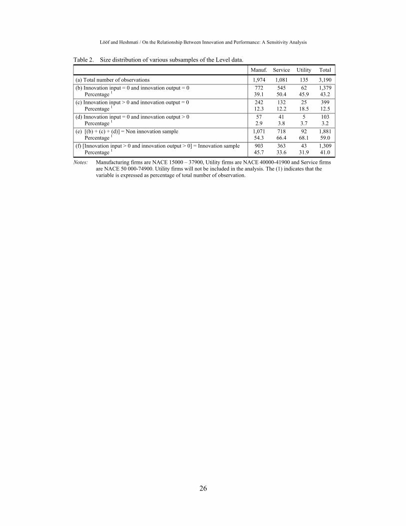
Lööf and Heshmati / On the Relationship Between Innovation and Performance: A Sensitivity Analysis
26
Table 2. Size distribution of various subsamples of the Level data. Manuf. Service Utility Total
(a) Total number of observations 1,974 1,081 135 3,190 (b) Innovation input = 0 and innovation output = 0 772 545 62 1,379
Percentage 1 39.1 50.4 45.9 43.2 (c) Innovation input > 0 and innovation output = 0 242 132 25 399
Percentage 1 12.3 12.2 18.5 12.5 (d) Innovation input = 0 and innovation output > 0 57 41 5 103
Percentage 1 2.9 3.8 3.7 3.2 (e) [(b) + (c) + (d)] = Non innovation sample 1,071 718 92 1,881
Percentage 1 54.3 66.4 68.1 59.0 (f) [Innovation input > 0 and innovation output > 0] = Innovation sample 903 363 43 1,309
Percentage 1 45.7 33.6 31.9 41.0
Notes: Manufacturing firms are NACE 15000 – 37900, Utility firms are NACE 40000-41900 and Service firms are NACE 50 000-74900. Utility firms will not be included in the analysis. The (1) indicates that the variable is expressed as percentage of total number of observation.
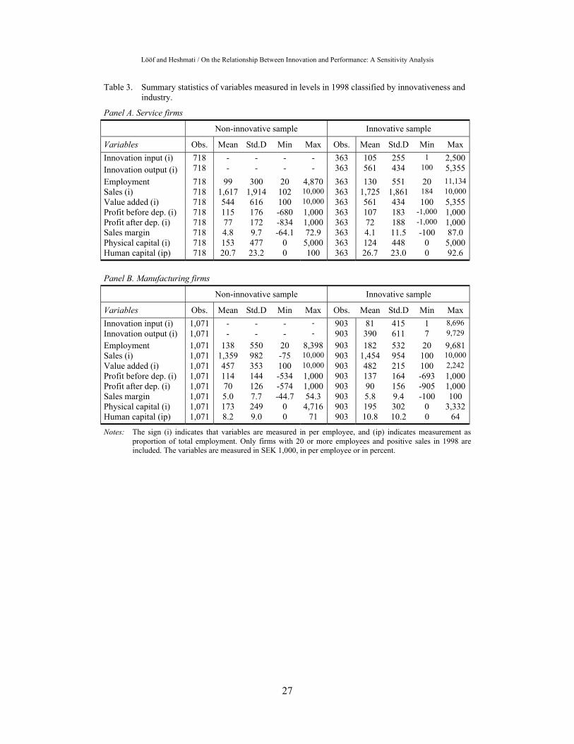
Lööf and Heshmati / On the Relationship Between Innovation and Performance: A Sensitivity Analysis
27
Table 3. Summary statistics of variables measured in levels in 1998 classified by innovativeness and industry.
Panel A. Service firms
Non-innovative sample Innovative sample
Variables Obs. Mean Std.D Min Max Obs. Mean Std.D Min Max Innovation input (i) 718 - - - - 363 105 255 1 2,500Innovation output (i) 718 - - - - 363 561 434 100 5,355Employment 718 99 300 20 4,870 363 130 551 20 11,134Sales (i) 718 1,617 1,914 102 10,000 363 1,725 1,861 184 10,000Value added (i) 718 544 616 100 10,000 363 561 434 100 5,355Profit before dep. (i) 718 115 176 -680 1,000 363 107 183 -1,000 1,000Profit after dep. (i) 718 77 172 -834 1,000 363 72 188 -1,000 1,000Sales margin 718 4.8 9.7 -64.1 72.9 363 4.1 11.5 -100 87.0 Physical capital (i) 718 153 477 0 5,000 363 124 448 0 5,000Human capital (ip) 718 20.7 23.2 0 100 363 26.7 23.0 0 92.6
Panel B. Manufacturing firms
Non-innovative sample Innovative sample
Variables Obs. Mean Std.D Min Max Obs. Mean Std.D Min Max Innovation input (i) 1,071 - - - - 903 81 415 1 8,696 Innovation output (i) 1,071 - - - - 903 390 611 7 9,729 Employment 1,071 138 550 20 8,398 903 182 532 20 9,681Sales (i) 1,071 1,359 982 -75 10,000 903 1,454 954 100 10,000Value added (i) 1,071 457 353 100 10,000 903 482 215 100 2,242 Profit before dep. (i) 1,071 114 144 -534 1,000 903 137 164 -693 1,000Profit after dep. (i) 1,071 70 126 -574 1,000 903 90 156 -905 1,000Sales margin 1,071 5.0 7.7 -44.7 54.3 903 5.8 9.4 -100 100 Physical capital (i) 1,071 173 249 0 4,716 903 195 302 0 3,332Human capital (ip) 1,071 8.2 9.0 0 71 903 10.8 10.2 0 64
Notes: The sign (i) indicates that variables are measured in per employee, and (ip) indicates measurement as proportion of total employment. Only firms with 20 or more employees and positive sales in 1998 are included. The variables are measured in SEK 1,000, in per employee or in percent.
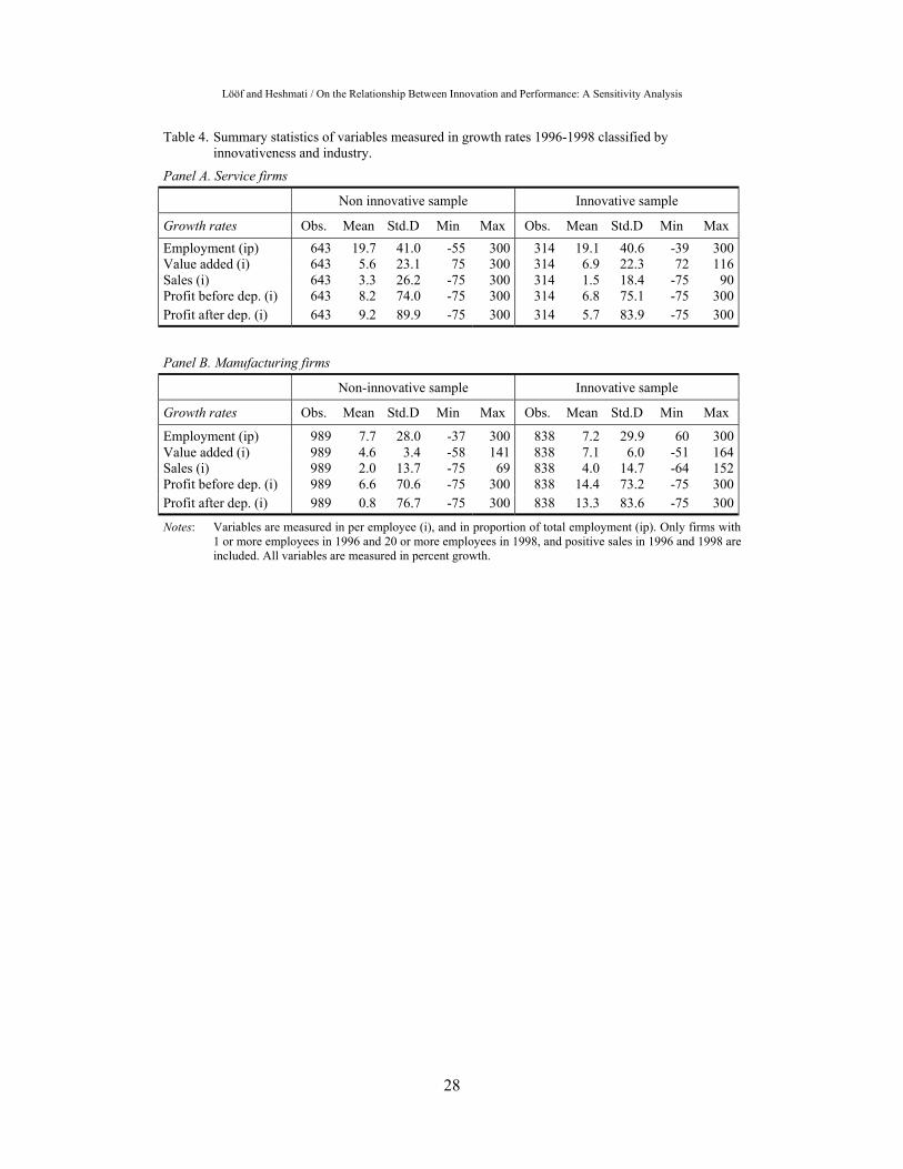
Lööf and Heshmati / On the Relationship Between Innovation and Performance: A Sensitivity Analysis
28
Table 4. Summary statistics of variables measured in growth rates 1996-1998 classified by innovativeness and industry.
Panel A. Service firms
Non innovative sample Innovative sample
Growth rates Obs. Mean Std.D Min Max Obs. Mean Std.D Min Max Employment (ip) 643 19.7 41.0 -55 300 314 19.1 40.6 -39 300Value added (i) 643 5.6 23.1 75 300 314 6.9 22.3 72 116Sales (i) 643 3.3 26.2 -75 300 314 1.5 18.4 -75 90Profit before dep. (i) 643 8.2 74.0 -75 300 314 6.8 75.1 -75 300Profit after dep. (i) 643 9.2 89.9 -75 300 314 5.7 83.9 -75 300
Panel B. Manufacturing firms
Non-innovative sample Innovative sample
Growth rates Obs. Mean Std.D Min Max Obs. Mean Std.D Min Max
Employment (ip) 989 7.7 28.0 -37 300 838 7.2 29.9 60 300Value added (i) 989 4.6 3.4 -58 141 838 7.1 6.0 -51 164Sales (i) 989 2.0 13.7 -75 69 838 4.0 14.7 -64 152Profit before dep. (i) 989 6.6 70.6 -75 300 838 14.4 73.2 -75 300Profit after dep. (i) 989 0.8 76.7 -75 300 838 13.3 83.6 -75 300
Notes: Variables are measured in per employee (i), and in proportion of total employment (ip). Only firms with 1 or more employees in 1996 and 20 or more employees in 1998, and positive sales in 1996 and 1998 are included. All variables are measured in percent growth.
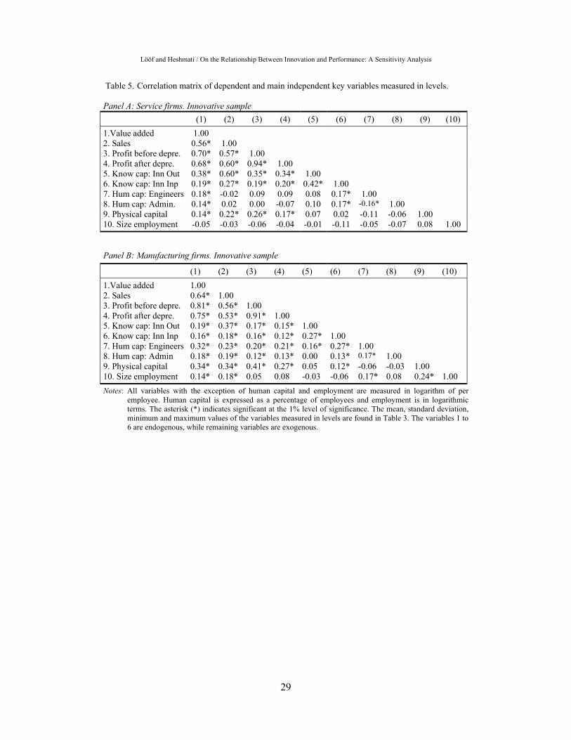
Lööf and Heshmati / On the Relationship Between Innovation and Performance: A Sensitivity Analysis
29
Table 5. Correlation matrix of dependent and main independent key variables measured in levels. Panel A: Service firms. Innovative sample (1) (2) (3) (4) (5) (6) (7) (8) (9) (10) 1.Value added 1.00 2. Sales 0.56* 1.00 3. Profit before depre. 0.70* 0.57* 1.00 4. Profit after depre. 0.68* 0.60* 0.94* 1.00 5. Know cap: Inn Out 0.38* 0.60* 0.35* 0.34* 1.00 6. Know cap: Inn Inp 0.19* 0.27* 0.19* 0.20* 0.42* 1.00 7. Hum cap: Engineers 0.18* -0.02 0.09 0.09 0.08 0.17* 1.00 8. Hum cap: Admin. 0.14* 0.02 0.00 -0.07 0.10 0.17* -0.16* 1.00 9. Physical capital 0.14* 0.22* 0.26* 0.17* 0.07 0.02 -0.11 -0.06 1.00 10. Size employment -0.05 -0.03 -0.06 -0.04 -0.01 -0.11 -0.05 -0.07 0.08 1.00
Panel B: Manufacturing firms. Innovative sample
(1) (2) (3) (4) (5) (6) (7) (8) (9) (10) 1.Value added 1.00 2. Sales 0.64* 1.00 3. Profit before depre. 0.81* 0.56* 1.00 4. Profit after depre. 0.75* 0.53* 0.91* 1.00 5. Know cap: Inn Out 0.19* 0.37* 0.17* 0.15* 1.00 6. Know cap: Inn Inp 0.16* 0.18* 0.16* 0.12* 0.27* 1.00 7. Hum cap: Engineers 0.32* 0.23* 0.20* 0.21* 0.16* 0.27* 1.00 8. Hum cap: Admin 0.18* 0.19* 0.12* 0.13* 0.00 0.13* 0.17* 1.00 9. Physical capital 0.34* 0.34* 0.41* 0.27* 0.05 0.12* -0.06 -0.03 1.00 10. Size employment 0.14* 0.18* 0.05 0.08 -0.03 -0.06 0.17* 0.08 0.24* 1.00 Notes: All variables with the exception of human capital and employment are measured in logarithm of per
employee. Human capital is expressed as a percentage of employees and employment is in logarithmic terms. The asterisk (*) indicates significant at the 1% level of significance. The mean, standard deviation, minimum and maximum values of the variables measured in levels are found in Table 3. The variables 1 to 6 are endogenous, while remaining variables are exogenous.
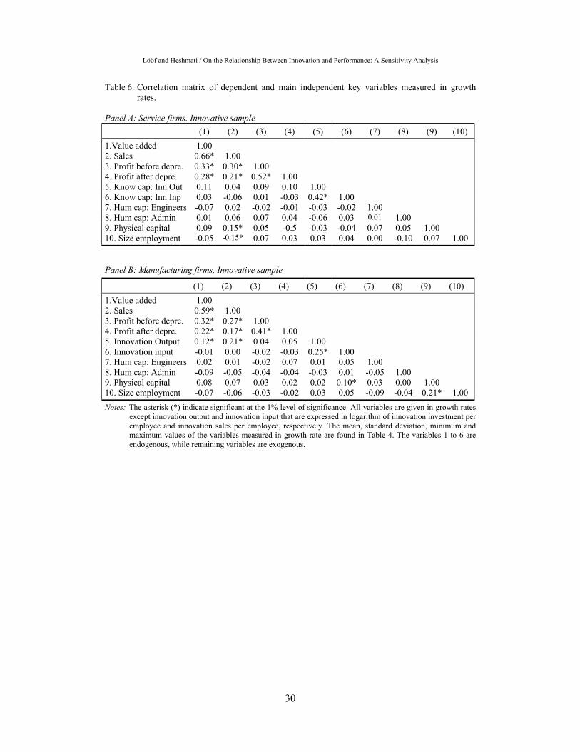
Lööf and Heshmati / On the Relationship Between Innovation and Performance: A Sensitivity Analysis
30
Table 6. Correlation matrix of dependent and main independent key variables measured in growth rates.
Panel A: Service firms. Innovative sample (1) (2) (3) (4) (5) (6) (7) (8) (9) (10) 1.Value added 1.00 2. Sales 0.66* 1.00 3. Profit before depre. 0.33* 0.30* 1.00 4. Profit after depre. 0.28* 0.21* 0.52* 1.00 5. Know cap: Inn Out 0.11 0.04 0.09 0.10 1.00 6. Know cap: Inn Inp 0.03 -0.06 0.01 -0.03 0.42* 1.00 7. Hum cap: Engineers -0.07 0.02 -0.02 -0.01 -0.03 -0.02 1.00 8. Hum cap: Admin 0.01 0.06 0.07 0.04 -0.06 0.03 0.01 1.00 9. Physical capital 0.09 0.15* 0.05 -0.5 -0.03 -0.04 0.07 0.05 1.00 10. Size employment -0.05 -0.15* 0.07 0.03 0.03 0.04 0.00 -0.10 0.07 1.00
Panel B: Manufacturing firms. Innovative sample
(1) (2) (3) (4) (5) (6) (7) (8) (9) (10) 1.Value added 1.00 2. Sales 0.59* 1.00 3. Profit before depre. 0.32* 0.27* 1.00 4. Profit after depre. 0.22* 0.17* 0.41* 1.00 5. Innovation Output 0.12* 0.21* 0.04 0.05 1.00 6. Innovation input -0.01 0.00 -0.02 -0.03 0.25* 1.00 7. Hum cap: Engineers 0.02 0.01 -0.02 0.07 0.01 0.05 1.00 8. Hum cap: Admin -0.09 -0.05 -0.04 -0.04 -0.03 0.01 -0.05 1.00 9. Physical capital 0.08 0.07 0.03 0.02 0.02 0.10* 0.03 0.00 1.00 10. Size employment -0.07 -0.06 -0.03 -0.02 0.03 0.05 -0.09 -0.04 0.21* 1.00 Notes: The asterisk (*) indicate significant at the 1% level of significance. All variables are given in growth rates
except innovation output and innovation input that are expressed in logarithm of innovation investment per employee and innovation sales per employee, respectively. The mean, standard deviation, minimum and maximum values of the variables measured in growth rate are found in Table 4. The variables 1 to 6 are endogenous, while remaining variables are exogenous.
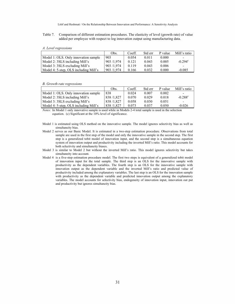
Lööf and Heshmati / On the Relationship Between Innovation and Performance: A Sensitivity Analysis
31
Table 7. Comparison of different estimation procedures. The elasticity of level (growth rate) of value added per employee with respect to log innovation output using manufacturing data.
A. Level regressions Obs. Coeff. Std err P value Mill’s ratio Model 1: OLS. Only innovation sample 903 0.054 0.011 0.000 - Model 2: 3SLS including Mill’s 903 /1,974 0.121 0.043 0.005 -0.294c Model 3: 3SLS excluding Mill’s 903 /1,974 0.119 0.043 0.006 - Model 4: 5-step, OLS including Mill’s 903 /1,974 0.166 0.032 0.000 -0.085 B. Growth rate regressions Obs. Coeff. Std err P value Mill’s ratio Model 1: OLS. Only innovation sample 838 0.024 0.007 0.002 - Model 2: 3SLS including Mill’s 838 /1,827 0.070 0.029 0.018 -0.288c Model 3: 3SLS excluding Mill’s 838 /1,827 0.058 0.030 0.051 - Model 4: 5-step, OLS including Mill’s 838 /1,827 0.073 0.037 0.050 -0.026 Notes: In Model 1 only innovative sample is used while in Models 2-4 total sample is used in the selection
equation. (c) Significant at the 10% level of significance. Model 1 is estimated using OLS method on the innovative sample. The model ignores selectivity bias as well as
simultaneity bias. Model 2 serves as our Basic Model. It is estimated in a two-step estimation procedure. Observations from total
sample are used in the first step of the model and only the innovative sample in the second step. The first step is a generalized tobit model of innovation input, and the second step is a simultaneous equation system of innovation output and productivity including the inverted Mill’s ratio. This model accounts for both selectivity and simultaneity biases.
Model 3 is similar to Model 2 but without the inverted Mill’s ratio. This model ignores selectivity but takes simultaneity into account.
Model 4 is a five-step estimation procedure model. The first two steps is equivalent of a generalized tobit model of innovation input for the total sample. The third step is an OLS for the innovative sample with productivity as the dependent variables. The fourth step is an OLS for the innovative sample with innovation output as the dependent variable and the inverted Mill’s ratio and predicted value of productivity included among the explanatory variables. The last step is an OLS for the innovation sample with productivity as the dependent variable and predicted innovation output among the explanatory variables. The model accounts for selectivity bias, endogeneity of innovation input, innovation out put and productivity but ignores simultaneity bias.

Lööf and Heshmati / On the Relationship Between Innovation and Performance: A Sensitivity Analysis
32
Table 8. Comparison of service and manufacturing firms. Estimation results are based on the basic model (Model 2) in level form.
Services Manufacturing
Coeff. Std Err Coeff. Std Err
A. Selection equation: The dependent variable is the likelihood of doing innovation investments Firm size: Employment 0.096 b 0.042 0.085 a 0.029 Physical capital: Log physical capital per employee 0.029 0.032 0.105 a 0.029 Human capital: Engineers as a proportion of employment 0.176 0.439 2.194 a 0.442 Human capital: Administrators as a proportion of emp. 0.192 0.232 -0.721 0.820 Strongly important factors for the competitiveness - High quality on the products 0.382 a 0.112 0.429 a 0.073 - High delivery security 0.295 a 0.111 0.100 0.074 - Trademark 0.136 0.127 0.234 a 0.008 - Knowledge content in the products 0.201 c 0.104 0.139 c 0.079 - Unique products 0.226 c 0.127 0.138 0.095
B. Innovation input equation: The dependent variable is log innovation investment per employee Firm size: Employment -0.367 a 0.078 -0.288 a 0.045 Physical capital 0.093 0.057 0.155 a 0.049 Export 0.116 a 0.030 0.076 0.018 Factors hampering innovation (d) - Problem with external cooperation on innovation 0.804 a 0.266 0.294 c 0.160 - lack of appropriate technology -0.744 a 0.280 0.021 0.106 - lack of personnel with appropriate skill 0.213 0.198 0.229 c 0.134
C. Innovation output equation: The dependent variable is log innovation sales per employee Innovation input: Log innovation input per employee 0.614 a 0.102 0.562 a 0.096 Inverted Mill’s ratio -0.197 0.286 -0.294 0.156 Firm size: log employment 0.140 c 0.079 0.024 0.044 Physical capital: Log physical capital per employee -0.013 0.057 -0.062 0.611 Growth rate on the firms main market: Strong. (d) 0.323 b 0.158 0.251a 0.090 Growth rate on the firms main market: Negative. (d) -0.492 0.318 -0.274 c 0.165 Strongly important source of knowledge for innovation (d) - professional conferences, meetings, journals 0.654 b 0.263 -0.070 0.188 - information technology -0.296 0.204 0.330 c 0.185 - suppliers 0.404c 0.235 0.194 0.127 - sources within the firm -0.244 c 0.138 -0.028 0.079 Prod. New to the market mainly dev. in coop. with others 0.274 b 0.135 -0.038 0.074 Prod. New to the firm mainly dev. Without coop. 0.455 a 0.140 0.364 a 0.083
D. Performance equation: The dependent variable is log value added per employee Innovation output: Log innovation sales per employee 0.093 b 0.047 0.121a 0.043 Physical capital: Log physical capital per employee 0.052 a 0.019 0.140 a 0.013 Human capital: Engineers as a proportion of employment 0.369 a 0.134 1.033 a 0.186 Human capital: Administrators as a proportion of emp. 0.491 b 0.235 1.314 a 0.384 Firm size: log employment 0.005 0.027 -0.007 0.013 Offensive innovation strategy. (d) 0.311 b 0.130 0.113 c 0.058 Defensive innovation strategy. (d) -0.129 b 0.058 -0.033 0.031 Process innovation. (d) -0.071 0.054 -0.071 0.026 Organizational innovation. (d) -0.069 0.057 -0.027 0.026
Notes: Significant at the 1% (a), 5% (b) and 10% (c) levels of significance. (d) Indicates dummy variable. Industry dummies (not reported here) are included in all four equations.

Lööf and Heshmati / On the Relationship Between Innovation and Performance: A Sensitivity Analysis
33
Table 9. Comparison of different classifications of firm performance. The elasticity of various measures of performance with respect to innovation output. The basic model (Model 2) is used.
Level: Dependent variables are: (1) log sales per employee, (2) log value added per employee, (3) sales margin defined as profit after depreciation as a percentage of total sales, (4) log profit before depreciation per employee, and (5) log profit after depreciation per employee.
Panel A. Service firms
Firm performance Obs Coef. t-value p-value
(1)Value added 363 0.093 1.965 0.049 (2) Sales 363 0.204 3.474 0.001 (3) Sales margin 363 0.013 1.142 0.250 (4) Profit before depreciation 317 0.168 1.474 0.140 (5) Profit after depreciation 280 0.364 2.555 0.011 Panel B. Manufacturing firms
Firm performance Obs Coef. t-value p-value
(1) Value added 903 0.121 2.801 0.005 (2) Sales 903 0.161 3.355 0.001 (3) Sales margin 903 0.020 1.792 0.073 (4) Profit before depreciation 815 0.267 2.689 0.007 (5) Profit after depreciation 745 0.453 3.543 0.000 Growth rate: Dependent variables are: (1) growth in value added per employee, (2) growth in sales per employee, (3) growth in profit before depreciation per employee, (4) growth in profit after depreciation per employee and (5) growth in employment. Panel C. Service firms
Firm performance Obs Coef. t-value p-value
(1) Value added 314 0.080 3.014 0.003 (2) Sales 314 -0.008 -0.397 0.691 (3) Profit before depreciation 288 0.240 2.543 0.011 (4) Profit after depreciation 262 0.218 1.994 0.046 (5) Employment 314 0.122 2.821 0.005
Panel D. Manufacturing firms
Firm performance Obs Coef. t-value p-value
(1) Value added 838 0.070 2.374 0.018 (2) Sales 838 0.054 0.020 0.008 (3) Profit before depreciation 765 0.078 0.794 0.427 (4) Profit after depreciation 698 0.148 1.041 0.298
(5) Employment 838 0.064 1.449 0.147
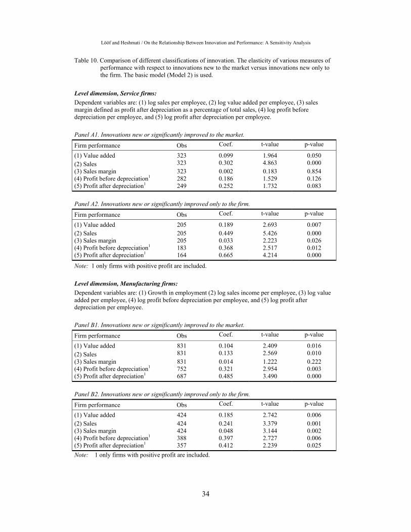
Lööf and Heshmati / On the Relationship Between Innovation and Performance: A Sensitivity Analysis
34
Table 10. Comparison of different classifications of innovation. The elasticity of various measures of performance with respect to innovations new to the market versus innovations new only to the firm. The basic model (Model 2) is used.
Level dimension, Service firms: Dependent variables are: (1) log sales per employee, (2) log value added per employee, (3) sales margin defined as profit after depreciation as a percentage of total sales, (4) log profit before depreciation per employee, and (5) log profit after depreciation per employee. Panel A1. Innovations new or significantly improved to the market.
Firm performance Obs Coef. t-value p-value
(1) Value added 323 0.099 1.964 0.050 (2) Sales 323 0.302 4.863 0.000 (3) Sales margin 323 0.002 0.183 0.854 (4) Profit before depreciation1 282 0.186 1.529 0.126 (5) Profit after depreciation1 249 0.252 1.732 0.083 Panel A2. Innovations new or significantly improved only to the firm.
Firm performance Obs Coef. t-value p-value
(1) Value added 205 0.189 2.693 0.007 (2) Sales 205 0.449 5.426 0.000 (3) Sales margin 205 0.033 2.223 0.026 (4) Profit before depreciation1 183 0.368 2.517 0.012 (5) Profit after depreciation1 164 0.665 4.214 0.000
Note: 1 only firms with positive profit are included. Level dimension, Manufacturing firms: Dependent variables are: (1) Growth in employment (2) log sales income per employee, (3) log value added per employee, (4) log profit before depreciation per employee, and (5) log profit after depreciation per employee. Panel B1. Innovations new or significantly improved to the market.
Firm performance Obs Coef. t-value p-value
(1) Value added 831 0.104 2.409 0.016 (2) Sales 831 0.133 2.569 0.010 (3) Sales margin 831 0.014 1.222 0.222 (4) Profit before depreciation1 752 0.321 2.954 0.003 (5) Profit after depreciation1 687 0.485 3.490 0.000 Panel B2. Innovations new or significantly improved only to the firm.
Firm performance Obs Coef. t-value p-value
(1) Value added 424 0.185 2.742 0.006 (2) Sales 424 0.241 3.379 0.001 (3) Sales margin 424 0.048 3.144 0.002 (4) Profit before depreciation1 388 0.397 2.727 0.006 (5) Profit after depreciation1 357 0.412 2.239 0.025 Note: 1 only firms with positive profit are included.
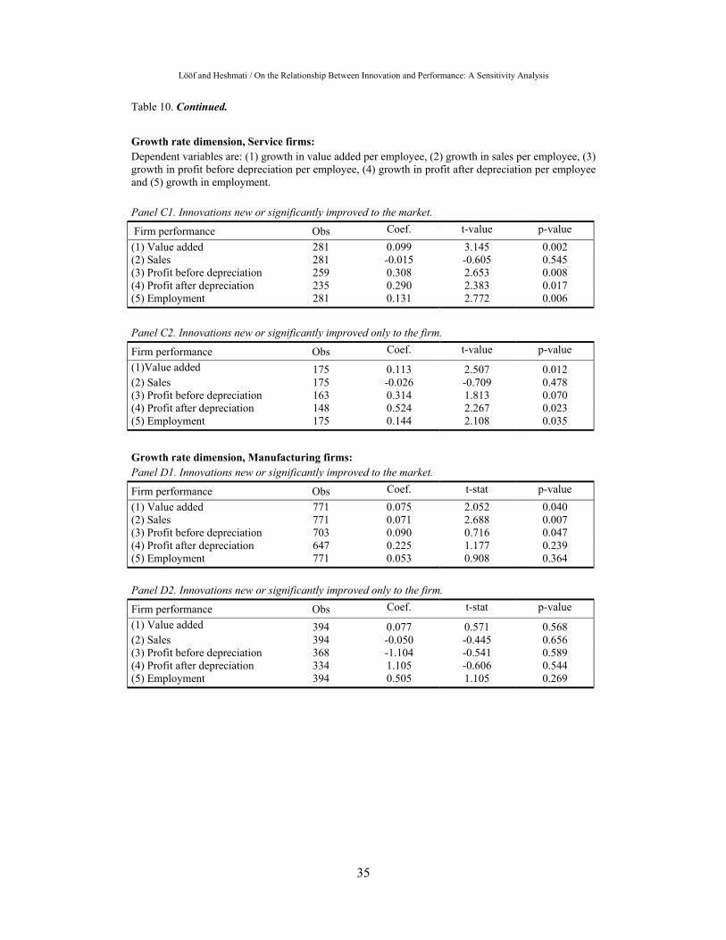
Lööf and Heshmati / On the Relationship Between Innovation and Performance: A Sensitivity Analysis
35
Table 10. Continued.
Growth rate dimension, Service firms: Dependent variables are: (1) growth in value added per employee, (2) growth in sales per employee, (3) growth in profit before depreciation per employee, (4) growth in profit after depreciation per employee and (5) growth in employment. Panel C1. Innovations new or significantly improved to the market.
Firm performance Obs Coef. t-value p-value (1) Value added 281 0.099 3.145 0.002 (2) Sales 281 -0.015 -0.605 0.545 (3) Profit before depreciation 259 0.308 2.653 0.008 (4) Profit after depreciation 235 0.290 2.383 0.017 (5) Employment 281 0.131 2.772 0.006
Panel C2. Innovations new or significantly improved only to the firm.
Firm performance Obs Coef. t-value p-value (1)Value added 175 0.113 2.507 0.012 (2) Sales 175 -0.026 -0.709 0.478 (3) Profit before depreciation 163 0.314 1.813 0.070 (4) Profit after depreciation 148 0.524 2.267 0.023 (5) Employment 175 0.144 2.108 0.035
Growth rate dimension, Manufacturing firms: Panel D1. Innovations new or significantly improved to the market.
Firm performance Obs Coef. t-stat p-value (1) Value added 771 0.075 2.052 0.040 (2) Sales 771 0.071 2.688 0.007 (3) Profit before depreciation 703 0.090 0.716 0.047 (4) Profit after depreciation 647 0.225 1.177 0.239 (5) Employment 771 0.053 0.908 0.364 Panel D2. Innovations new or significantly improved only to the firm.
Firm performance Obs Coef. t-stat p-value (1) Value added 394 0.077 0.571 0.568 (2) Sales 394 -0.050 -0.445 0.656 (3) Profit before depreciation 368 -1.104 -0.541 0.589 (4) Profit after depreciation 334 1.105 -0.606 0.544 (5) Employment 394 0.505 1.105 0.269

Lööf and Heshmati / On the Relationship Between Innovation and Performance: A Sensitivity Analysis
36
Table 11. Comparison of different data sources on sales and employment and censoring of outliers observations. The elasticity of sales per employee with respect to innovation output. The basic model (Model 2) is used.
Level regression Growth rate regression Services Manufacturing Services Manufacturing Obs Estimate Obs Estimate Obs Estimate Obs EstimateRegister data: Censored 363 0.269 a 903 0.163 a 314 0.125 b 838 0.050 b Noncensored 363 0.270 a 903 0.161 a 314 -0.016 838 0.050 b Survey data: Censored 319 0.161 b 820 0.195 a 266 0.054 674 0.039 Noncensored 319 0.155 c 820 0.199 a 266 0.085 b 674 0.046
Notes: Significant at the 1% (a), 5% (b) and 10% (c) levels of significance.


