On the Conceptual Engine Design and Sizing Tool
100
On the Conceptual En- gine Design and Sizing Tool MSc Thesis J.C. Tiemstra Technische Universiteit Delft
Transcript of On the Conceptual Engine Design and Sizing Tool

On the Conceptual En-gine Design and SizingToolMSc Thesis
J.C. Tiemstra
Tech
nische
Unive
rsite
itDelft


On the Conceptual Engine Design andSizing Tool
MSc Thesis
by
J.C. Tiemstra
in partial fulfillment of the requirements for the degree of
Master of Sciencein Aerospace Engineering
at the Delft University of Technology,to be defended publicly on Friday February 2, 2017 at 2:00 PM.
Student number: 4012569Project duration: September 15, 2015 – February 3, 2016Supervisor: Dr. A. G. RaoThesis committee: Dr. A. G. Rao, TU Delft (FPP),
Dr. ir. C. Lettieri, TU Delft (FPP),Dr. R. Pecnik, TU Delft (3ME)
An electronic version of this thesis is available at http://repository.tudelft.nl/.

Extensive summaryAir travel has been an advancing branch in the transportation market and has proven to be resilientto external financial shocks over the years. A recent market study by Airbus showed that the aviationmarket has been steadily growing at an approximate rate of 5% each year for the past two decades. Itis expected that this growth will be sustained for at least another 20 years. Consequently, the AdvisoryCouncil for Aeronautics Research in Europe (ACARE) presented a report on the environmental impactof the aviation industry and concluded that large improvements are needed with respect to reducingemissions from the aviation industry in order to comply with international standards. ACARE hasset several (non-binding) goals for the years 2020 and 2050, which will be primarily focussed on thereduction of three types of aircraft emissions: noise production, 𝐶𝑂 emissions, and 𝑁𝑂 , 𝐶𝑂 & 𝑈𝐻𝐶emissions. These goals are referred to as “extremely challenging” by ACARE, requiring revolutionarychange in the aviation industry.
Incorporating the environmental aspect has increased the complexity of the engine design process,while performance targets are evermore demanding. The envisioned improvements proposed by ACARErequire fast paced advancements in engine technology that reach beyond the capabilities of current en-gine design methods. Therefore, new methods that allow for quick investigation of engine conceptualdesigns are needed. Current design tools usually focus on optimizing the aerothermodynamic perfor-mance of the engine, while another important factor for aircraft propulsion systems, the engine weight,is often not integrated into this design process. It is important to already make accurate weight esti-mates of engine components in the conceptual design phase, as inaccuracies may lead to compulsorydesign changes in later design phases. Weight estimations early on in the design cycle of the engine mayresult in an overall more fuel efficient engine design and thus help reaching the goals set by ACARE.
The engine conceptual design and sizing tool developed in this thesis focuses on the fan stage andlow pressure compressor of a twin-spool high-bypass ratio turbofan engine. The tool will be used todetermine the effect of increasing the fan tip diameter on the aerodynamic performance, its total weightand the noise production of the engine. Three separate modules are designed for this purpose. Anaerodynamic module is used for the aero- and thermodynamic design and analysis of the components.In the module, the fan stage is designed using a Blade-Element Method (BEM), while a mean-linedesign is chosen for the design of the low pressure compressor. Secondly, a weight estimation moduleis integrated that focusses on the structural design of all components, including component fatiguebehaviour, and determines the weight of each component. Finally, a noise prediction module is used todetermine the noise spectrum of the engine. According to the International Civil Aviation Orginazation(ICAO) regulations, the noise performance of the engine is determined as measured by an observer onthe ground using a fly-over simulation. All modules are first validated using available engine data froma General Electric CF6-80C2/B6F engine, after which the research question is answered.
Since only the low pressure compressor components are considered in this research, further inves-tigation is needed to integrate other engine components in the design cycle and arrive at a full-scaleconceptual engine design and sizing tool.
iii


AcknowledgementsOver the past few months I received help and support from many people, and all of them have con-tributed to where I am today. I must say that the journey has been more intense than I suspected,and it is the people that were there for me repeatedly along the road that I want to address here witha special word of thanks.
First I would like to thank my thesis advisor and daily supervisor, Dr. Arvind Gangoli Rao, forcreating the opportunity to undertake this project with him. During the Master’s programme, Arvindhas raised my interest for the field of aeroengine propulsion by his passionate lecturing on enginerelated topics. Working together on this project has been a very positive experience for me and I wantto thank him for his positive attitude, everlasting patience and valuable advice throughout the project.I appreciate it how I was consistently allowed to let this thesis be my own work, with you steering mein the right direction whenever necessary.
I would also like to thank all people that helped me with the validation survey of this thesis project.Without their passionate participation and hospitality of receiving me on-site, this validation surveycould not have been conducted. Unfortunately I cannot mention any names as the source of the datahas to remain anonymous, but their help is really appreciated.
Furthermore, I want to thank my friends for their emotional support in the process of making thisthesis. I want to thank my girlfriend Amaya for all her love and support these past few months. Alsomy friends, with whom I shared good times and somehow made this long project feel like passed inno-time.
Last but not least, I would like to thank my family for their loving support throughout the wholeprocess. A special word of thanks goes out to my parents, who have always been there for me, whoalways trusted in me and had no doubt I would succeed even in times when I was going throughmoral slumps. Their motivational words have always kept me on track and helped me to put things inperspective.
v


Contents
List of Figures iii
List of Tables v
1 Introduction 11.1 Problem statement . . . . . . . . . . . . . . . . . . . . . . . . . . . . . . . . . . . . . . . 11.2 Thesis objective . . . . . . . . . . . . . . . . . . . . . . . . . . . . . . . . . . . . . . . . . 21.3 Report outline . . . . . . . . . . . . . . . . . . . . . . . . . . . . . . . . . . . . . . . . . 4
2 General Considerations 52.1 Turbofan configuration & lay-out . . . . . . . . . . . . . . . . . . . . . . . . . . . . . . . 5
2.1.1 Spool configurations . . . . . . . . . . . . . . . . . . . . . . . . . . . . . . . . . . 52.1.2 Compressor types . . . . . . . . . . . . . . . . . . . . . . . . . . . . . . . . . . . . 62.1.3 Flow mixing configurations. . . . . . . . . . . . . . . . . . . . . . . . . . . . . . . 62.1.4 Chosen configuration . . . . . . . . . . . . . . . . . . . . . . . . . . . . . . . . . . 6
2.2 Turbofan components . . . . . . . . . . . . . . . . . . . . . . . . . . . . . . . . . . . . . 62.3 Design Point . . . . . . . . . . . . . . . . . . . . . . . . . . . . . . . . . . . . . . . . . . 82.4 Modules . . . . . . . . . . . . . . . . . . . . . . . . . . . . . . . . . . . . . . . . . . . . . 8
2.4.1 Aerothermodynamic performance . . . . . . . . . . . . . . . . . . . . . . . . . . . 92.4.2 Weight estimation . . . . . . . . . . . . . . . . . . . . . . . . . . . . . . . . . . . 92.4.3 Noise prediction. . . . . . . . . . . . . . . . . . . . . . . . . . . . . . . . . . . . . 10
2.5 Validation . . . . . . . . . . . . . . . . . . . . . . . . . . . . . . . . . . . . . . . . . . . . 11
3 Aerodynamics 133.1 Governing equations and assumptions . . . . . . . . . . . . . . . . . . . . . . . . . . . . . 133.2 Non-dimensional performance parameters . . . . . . . . . . . . . . . . . . . . . . . . . . . 143.3 Gas path analysis . . . . . . . . . . . . . . . . . . . . . . . . . . . . . . . . . . . . . . . . 16
3.3.1 Design methods . . . . . . . . . . . . . . . . . . . . . . . . . . . . . . . . . . . . . 163.3.2 Annulus geometry . . . . . . . . . . . . . . . . . . . . . . . . . . . . . . . . . . . 163.3.3 Cascade design . . . . . . . . . . . . . . . . . . . . . . . . . . . . . . . . . . . . . 173.3.4 Velocity triangles . . . . . . . . . . . . . . . . . . . . . . . . . . . . . . . . . . . . 183.3.5 Vortex design . . . . . . . . . . . . . . . . . . . . . . . . . . . . . . . . . . . . . . 183.3.6 Incidence angle . . . . . . . . . . . . . . . . . . . . . . . . . . . . . . . . . . . . . 203.3.7 Deviation angle . . . . . . . . . . . . . . . . . . . . . . . . . . . . . . . . . . . . . 213.3.8 Loss sources . . . . . . . . . . . . . . . . . . . . . . . . . . . . . . . . . . . . . . . 22
3.4 Fan Analysis & Design . . . . . . . . . . . . . . . . . . . . . . . . . . . . . . . . . . . . . 233.4.1 Design methodology . . . . . . . . . . . . . . . . . . . . . . . . . . . . . . . . . . 233.4.2 Inlet calculations . . . . . . . . . . . . . . . . . . . . . . . . . . . . . . . . . . . . 253.4.3 Pressure losses . . . . . . . . . . . . . . . . . . . . . . . . . . . . . . . . . . . . . 28
3.5 LPC analysis & design . . . . . . . . . . . . . . . . . . . . . . . . . . . . . . . . . . . . . 303.5.1 Design methodology . . . . . . . . . . . . . . . . . . . . . . . . . . . . . . . . . . 303.5.2 Inlet calculations . . . . . . . . . . . . . . . . . . . . . . . . . . . . . . . . . . . . 313.5.3 Pressure losses . . . . . . . . . . . . . . . . . . . . . . . . . . . . . . . . . . . . . 32
4 Structural analysis & Weight 374.1 Materials . . . . . . . . . . . . . . . . . . . . . . . . . . . . . . . . . . . . . . . . . . . . 374.2 Fatigue life . . . . . . . . . . . . . . . . . . . . . . . . . . . . . . . . . . . . . . . . . . . 38
4.2.1 Design methodology . . . . . . . . . . . . . . . . . . . . . . . . . . . . . . . . . . 384.2.2 Estimated stress-life . . . . . . . . . . . . . . . . . . . . . . . . . . . . . . . . . . 40
i
ii Contents
4.3 Blades . . . . . . . . . . . . . . . . . . . . . . . . . . . . . . . . . . . . . . . . . . . . . . 424.4 Disks . . . . . . . . . . . . . . . . . . . . . . . . . . . . . . . . . . . . . . . . . . . . . . 444.5 Casing . . . . . . . . . . . . . . . . . . . . . . . . . . . . . . . . . . . . . . . . . . . . . . 46
4.5.1 Pressure containment. . . . . . . . . . . . . . . . . . . . . . . . . . . . . . . . . . 464.5.2 Blade containment . . . . . . . . . . . . . . . . . . . . . . . . . . . . . . . . . . . 47
4.6 Shaft. . . . . . . . . . . . . . . . . . . . . . . . . . . . . . . . . . . . . . . . . . . . . . . 474.7 Spinner cone . . . . . . . . . . . . . . . . . . . . . . . . . . . . . . . . . . . . . . . . . . 47
5 Noise Estimation 495.1 Noise prediction methods . . . . . . . . . . . . . . . . . . . . . . . . . . . . . . . . . . . 495.2 Heidmann’s method . . . . . . . . . . . . . . . . . . . . . . . . . . . . . . . . . . . . . . 49
5.2.1 Broadband noise . . . . . . . . . . . . . . . . . . . . . . . . . . . . . . . . . . . . 505.2.2 Discrete tone noise . . . . . . . . . . . . . . . . . . . . . . . . . . . . . . . . . . . 515.2.3 Combination tone noise . . . . . . . . . . . . . . . . . . . . . . . . . . . . . . . . 51
5.3 Improved Heidmann’s method . . . . . . . . . . . . . . . . . . . . . . . . . . . . . . . . . 515.4 ESDU method . . . . . . . . . . . . . . . . . . . . . . . . . . . . . . . . . . . . . . . . . 525.5 Take-off simulation . . . . . . . . . . . . . . . . . . . . . . . . . . . . . . . . . . . . . . . 525.6 Noise descriptors . . . . . . . . . . . . . . . . . . . . . . . . . . . . . . . . . . . . . . . . 53
6 Module validation 556.1 Aerodynamic module . . . . . . . . . . . . . . . . . . . . . . . . . . . . . . . . . . . . . . 556.2 Structural analysis & weight estimation module . . . . . . . . . . . . . . . . . . . . . . . 606.3 Noise module . . . . . . . . . . . . . . . . . . . . . . . . . . . . . . . . . . . . . . . . . . 62
7 Results & Conclusions 677.1 Effect of increasing fan tip diameter . . . . . . . . . . . . . . . . . . . . . . . . . . . . . . 677.2 Effect of spool speed . . . . . . . . . . . . . . . . . . . . . . . . . . . . . . . . . . . . . . 68
8 Recommendations 738.1 Aerodynamics module . . . . . . . . . . . . . . . . . . . . . . . . . . . . . . . . . . . . . 738.2 Structural & analysis module . . . . . . . . . . . . . . . . . . . . . . . . . . . . . . . . . 738.3 Noise module . . . . . . . . . . . . . . . . . . . . . . . . . . . . . . . . . . . . . . . . . . 74
A Loss coefficient correlations 75
Bibliography 77
List of Figures
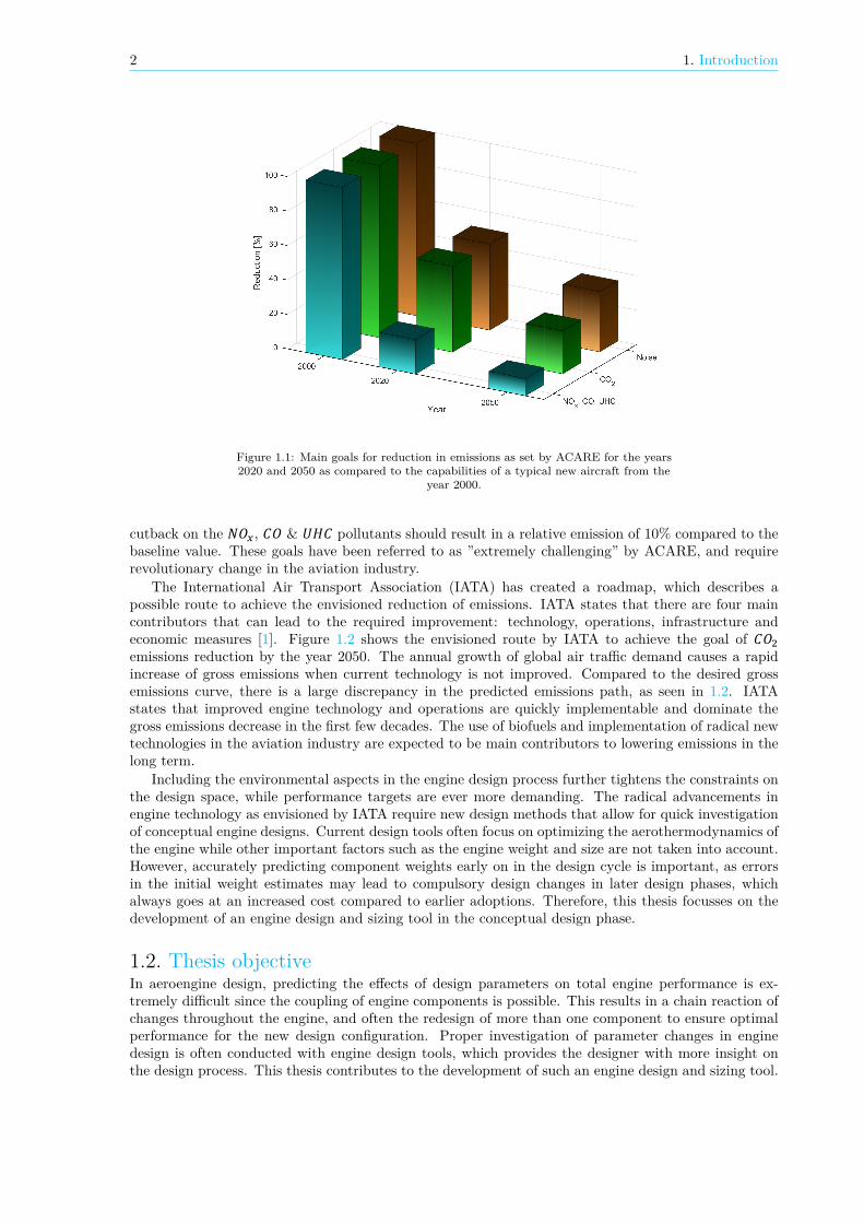
1.1 Main goals for reduction in emissions as set by ACARE for the years 2020 and 2050 ascompared to the capabilities of a typical new aircraft from the year 2000. . . . . . . . . 2
1.2 Schematic 𝐶𝑂 emissions reduction roadmap. Source:[1] . . . . . . . . . . . . . . . . . . 3
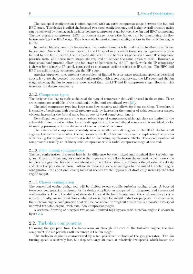
2.1 CF6-80C2 Sectional Drawing. Source: [2] . . . . . . . . . . . . . . . . . . . . . . . . . . 72.2 Typical mission profile for civil airfraft. Source: [3] . . . . . . . . . . . . . . . . . . . . . 82.3 Engine weight component break-down. . . . . . . . . . . . . . . . . . . . . . . . . . . . . 102.4 Comparison of noise sources and magnitudes for low- and high-BPR turbofan engines.
Source: [4] . . . . . . . . . . . . . . . . . . . . . . . . . . . . . . . . . . . . . . . . . . . 102.5 CF6-80C2 engine. Source: GE Aviation . . . . . . . . . . . . . . . . . . . . . . . . . . . 112.6 CFM56-7B engine. Source: CFM International . . . . . . . . . . . . . . . . . . . . . . . 11
3.1 Flowpath geometry designs. . . . . . . . . . . . . . . . . . . . . . . . . . . . . . . . . . . 173.2 Three popular compressor cascades. . . . . . . . . . . . . . . . . . . . . . . . . . . . . . 183.3 Fan blade angle nomenclature. Source: [5] . . . . . . . . . . . . . . . . . . . . . . . . . . 193.4 Velocity triangle nomenclature. Source: [5] . . . . . . . . . . . . . . . . . . . . . . . . . 193.5 Optimum incidence angle and stall boundaries on the cascade loss curve. Source: [6] . . 203.6 Comparison of rotor incidence angle prediction methods using NASA rotor data (table
3.4). . . . . . . . . . . . . . . . . . . . . . . . . . . . . . . . . . . . . . . . . . . . . . . . 213.7 Comparison of stator incidence angle prediction methods using NASA rotor data (table
3.4). . . . . . . . . . . . . . . . . . . . . . . . . . . . . . . . . . . . . . . . . . . . . . . . 213.8 Comparison of rotor deviation angle prediction methods using NASA rotor data (table
3.4). . . . . . . . . . . . . . . . . . . . . . . . . . . . . . . . . . . . . . . . . . . . . . . . 223.9 Comparison of stator deviation angle prediction methods using NASA rotor data (table
3.4). . . . . . . . . . . . . . . . . . . . . . . . . . . . . . . . . . . . . . . . . . . . . . . . 223.10 Iterative solving method for blade angles. . . . . . . . . . . . . . . . . . . . . . . . . . . 223.11 Development of tip, hub and endwall vortices in fan rotor and stator blade channels.
Source: [7] . . . . . . . . . . . . . . . . . . . . . . . . . . . . . . . . . . . . . . . . . . . 233.12 Flow fields in a compressor cascade with loss sources indicated. Source: [8] . . . . . . . 233.13 Fan stage. Source: GrabCAD . . . . . . . . . . . . . . . . . . . . . . . . . . . . . . . . . 243.14 Fan design . . . . . . . . . . . . . . . . . . . . . . . . . . . . . . . . . . . . . . . . . . . . 263.15 Iterative solving method for fan rotor design. . . . . . . . . . . . . . . . . . . . . . . . . 273.16 Iterative solving method for inlet axial velocity, 𝐶 . . . . . . . . . . . . . . . . . . . . . 283.17 Low pressure compressor stage. Source: GrabCAD . . . . . . . . . . . . . . . . . . . . . 303.18 Low pressure compressor design map. . . . . . . . . . . . . . . . . . . . . . . . . . . . . 313.19 Inlet specific flow vs. Mach number with typical LPC inlet conditions indicated. . . . . 32
4.1 Temperature effect on yield and ultimate strength. . . . . . . . . . . . . . . . . . . . . . 384.2 Stress amplitude ratio. . . . . . . . . . . . . . . . . . . . . . . . . . . . . . . . . . . . . . 394.3 Fatigue safety margin methods. . . . . . . . . . . . . . . . . . . . . . . . . . . . . . . . . 394.4 Modified S-N curves for steel component. Source: [9] . . . . . . . . . . . . . . . . . . . . 404.5 S-N data curve fitting vs. fatigue life estimation . . . . . . . . . . . . . . . . . . . . . . . 424.6 Blade build up. Source: [10] . . . . . . . . . . . . . . . . . . . . . . . . . . . . . . . . . . 434.7 Rotating disk stress analysis. Source: [11] . . . . . . . . . . . . . . . . . . . . . . . . . . 44
5.1 Rotor-stator interaction discrete tone harmonic levels and fundamental tone level cut-off.Source: [5] . . . . . . . . . . . . . . . . . . . . . . . . . . . . . . . . . . . . . . . . . . . 51
5.2 Take-off procedure. Source: [5] . . . . . . . . . . . . . . . . . . . . . . . . . . . . . . . . 535.3 Lateral noise measurement location. Source: [5] . . . . . . . . . . . . . . . . . . . . . . . 53
iii

iv List of Figures
5.4 Distance history for 767-300ER take-off procedure. . . . . . . . . . . . . . . . . . . . . . 535.5 Angle history for 767-300ER take-off procedure. . . . . . . . . . . . . . . . . . . . . . . . 53
6.1 Optimized fan results for CFM56-7B engine at take-off design point. . . . . . . . . . . . 566.2 Optimized fan blade shape of a CFM56-7B engine at take-off design point, with section
cuts along the streamline at hub, splitter and tip radii. . . . . . . . . . . . . . . . . . . . 576.3 Optimized fan results for CFM56-7B engine at take-off design point, with alternative
DeHaller design limit of 0.6. . . . . . . . . . . . . . . . . . . . . . . . . . . . . . . . . . . 586.4 Optimized fan blade shape of a CFM56-7B engine at take-off design point, with alterna-
tive DeHaller design limit of 𝐷𝐻 ≥ 0.6. Section cuts shown along the streamline at hub,splitter, and tip radii, and horizontal projected section cut at the splitter. . . . . . . . . 59
6.5 CFM56-7B fan blade validation section at approximately one-third of blade height. . . . 596.6 Fan rotor blade off-design performance with design point indicated. . . . . . . . . . . . . 606.7 Disk stress analysis validation using T-AXI Disk . . . . . . . . . . . . . . . . . . . . . 616.8 Disk stress analysis validation using T-AXI Disk . . . . . . . . . . . . . . . . . . . . . 616.9 CFM56-7 Sectional drawing overlay. Source: [12] . . . . . . . . . . . . . . . . . . . . . . 626.10 CFM56-7 LPC componenents exported to 3D output. . . . . . . . . . . . . . . . . . . . 636.11 Fan inlet and exhaust noise spectral comparison of different noise prediction methods for
a range of directivity angles measured from engine inlet axis at a 150 𝑓𝑡 (45.27 𝑚) radius. 646.12 Take-off fly-over simulation vs. certified engine data. Source: [13] . . . . . . . . . . . . . 666.13 Take-off lateral simulation vs. certified engine data. Source: [13] . . . . . . . . . . . . . 66
7.1 Rotor adiabatic performance . . . . . . . . . . . . . . . . . . . . . . . . . . . . . . . . . 677.2 Relative total engine weight . . . . . . . . . . . . . . . . . . . . . . . . . . . . . . . . . . 677.3 Tip diameter effect on the fly-over lateral measurement EPNL. . . . . . . . . . . . . . . 687.4 Tip diameter effect on the fly-over longitudinal measurement EPNL. . . . . . . . . . . . 687.5 The effect of spool speed on the bypass and core adiabatic efficiency 𝜂 for a range of
bypass ratios. . . . . . . . . . . . . . . . . . . . . . . . . . . . . . . . . . . . . . . . . . . 697.6 Effect of spool speed on total mass 𝑚 for a range of bypass ratios. . . . . . . . . . . . 697.7 Component mass break-down for varying spool speed at design BPR. . . . . . . . . . . . 707.8 Effect of spool speed on the aerodynamic efficiency and component mass. . . . . . . . . 707.9 Effect of bypass ratio on the flow path geometry and component mass sizes at design
spool speed. . . . . . . . . . . . . . . . . . . . . . . . . . . . . . . . . . . . . . . . . . . . 71
A.1 Shock loss coefficient, 𝜁 , as a function of immersion ratio, 𝐻, and modified diffusionparameter, 𝐷 . . . . . . . . . . . . . . . . . . . . . . . . . . . . . . . . . . . . . . . . . . 75
A.2 Profile loss coefficient, 𝜁 , as a function of immersion ratio, 𝐻, and modified diffusionparameter, 𝐷 . . . . . . . . . . . . . . . . . . . . . . . . . . . . . . . . . . . . . . . . . . 75

List of Tables
2.1 Typical component sizing conditions. Source: [14] . . . . . . . . . . . . . . . . . . . . . 82.2 Overview of aerothermodynamic performance optimisation codes. Source: [15] . . . . . 92.3 Overview of component based weight estimation methods. . . . . . . . . . . . . . . . . . 92.4 Overview of implemented noise prediction methods in Soprano. Source: [16] . . . . . . . 112.5 Characteristic data for validation engines CF6-80C2/B6 (Roux [17]) and CFM56-7B24
(engine testrun data). . . . . . . . . . . . . . . . . . . . . . . . . . . . . . . . . . . . . . 12
3.1 Blockage factor. [18] . . . . . . . . . . . . . . . . . . . . . . . . . . . . . . . . . . . . . . 173.2 Airfoil and velocity triangle nomenclature. . . . . . . . . . . . . . . . . . . . . . . . . . . 183.3 Special cases for general vortex design. . . . . . . . . . . . . . . . . . . . . . . . . . . . . 203.4 Experimental data used for validation of incidence angle and deviation angle prediction
methods. . . . . . . . . . . . . . . . . . . . . . . . . . . . . . . . . . . . . . . . . . . . . . 213.5 Fan inlet input parameters. . . . . . . . . . . . . . . . . . . . . . . . . . . . . . . . . . . 243.6 LPC inlet input parameters. . . . . . . . . . . . . . . . . . . . . . . . . . . . . . . . . . . 313.7 Constants 𝐾 as mentioned in the diffusion factor calculations . . . . . . . . . . . . . . . 34
4.1 Aeroengine material properties. Source: [19–21] . . . . . . . . . . . . . . . . . . . . . . . 384.2 Baseline fatigue strength, 𝑆 , and loading factor, 𝐶 , based on the material and loading
conditions. . . . . . . . . . . . . . . . . . . . . . . . . . . . . . . . . . . . . . . . . . . . . 414.3 Reliability factor, 𝐶 . . . . . . . . . . . . . . . . . . . . . . . . . . . . . . . . . . . . . . 414.4 Baseline bending fatigue limit, 𝑆 , and cycle limit, 𝑁 . . . . . . . . . . . . . . . . . . 414.5 Component materials and fatigue design input parameters. . . . . . . . . . . . . . . . . 42
5.1 Take-off simulation input parameters. . . . . . . . . . . . . . . . . . . . . . . . . . . . . 52
6.1 Input for noise spectrum level calculations of the CF6-80C2 engine. . . . . . . . . . . . . 63
v

Nomenclature
Symbols
Symbol Units Description𝛼 1/K Coefficient of thermal expansion𝛼 deg Absolute flow angle𝛽 deg Relative flow angleΓ∗ - Blade dimensionless circulation parameter𝛾 deg Stagger angle𝛾 - Ratio of specific heats𝛿 deg Deviation angle𝛿 deg Deviation angle for zero incidence angle𝛿∗ m Boundary layer displacement thickness𝜖 - Polytropic efficiency𝜁 - Loss parameter𝜁 - Total loss parameter𝜁 - Mach number correction factor𝜁 - Flow area contraction correction factor𝜁 - Reynold’s number correction factor𝜂 - Isentropic efficiency𝜃 deg Camber angle𝜃 m Boundary layer momentum thickness𝜄 deg Incidence angle𝜅 deg Metal angle𝜅 m Peak-to-valley surface roughness𝜇 - Axial velocity ratio𝜇 - Weinig mu-factor𝜈 - Rotational velocity ratio𝜈 - Poisson’s ratio𝜉 - Mach number correction factor𝜉 - Flow area contraction correction factor𝜉 - Reynold’s number correction factor𝜋 - Total pressure ratio𝜌 kg/m Density𝜎 - Blade cascade solidity ratio𝜎 MPa Hoop stress𝜎 . MPa Yield strength𝜎 MPa Radial stress𝜎 MPa Ultimate tensile strength𝜎 MPa Von Mises stress𝜎 MPa Yield strength𝜏 - Total temperature ratio𝜏 m Blades clearance gapΦ - Stage flow coefficientΨ - Stage loading coefficientΩ rad/s Angular velocity𝑎 m Blade chamber𝐴 m Area(𝑎/𝑐) - Blade chamber to chord ratio𝑏 - Tuning factor
vii
viii List of Tables
𝑐, 𝐶 m/s Absolute flow speed𝑐 m Blade chord(𝑐/𝜅) - Blade chord to surface roughness(𝑐/ℎ) - Blade aspect ratio𝑐 J/(kg.K) Specific heat capacity𝐶 Blade lift coefficient𝐷 - Diffusion factor𝐷 m Diameter𝐷 - Equivalent diffusion factor𝐷 - Modified diffusion factor𝑑𝐻 - “De Haller”-number𝐸 GPa Young’s modulus𝐸 J Blade kinetic energy𝐸𝑃𝑁𝐿 dB Equivalent Perceived Noise Level𝐹 N Thrust force𝐹𝐻𝑉 J Fuel heating valueℎ m Heightℎ J/(kg.K) Enthalpyℎ J/(kg.K) Total enthalpy𝐻 - Immersion factor𝐻 - Boundary layer trailing edge shape factor(Δ𝐻/𝑛𝑈 ) - Mean stage loading𝑖 deg Incidence angle𝑖 , deg Incidence angle based on 10% blade thickness(𝐾 ) - Thickness correction factor𝐾 - Blockage factor𝐾 - Compressibility correction factor𝐾 - Thickness correction factor𝐾 - Shape correction factor𝐾 - Thickness correction factor𝑙 - Specific mechanical energy𝑙 m Total stage length𝐿𝐻𝑉 J Lower heating value𝑚 kg Mass𝑚 - Slope of linear relation between deviation angle and camber angle𝑚 - Slope of linear relation between deviation angle and camber angle for
solidity ratio of 1 kg/s Mass flow𝑀 - Mach number𝑀𝐹𝑃 - Mass flow parameter𝑛 - Number of blades𝑛 - Number of stages𝑃 Pa Pressure𝑟 m Radius𝑟 m Hub radius𝑟 m Tip radius𝑅 J/(kg.K) Specific gas constant𝑅𝑒 - Reynold’s number𝑠 J/(kg.K) Entropy𝑠 m Blade spacing(𝑆/𝑐) - Pitch chord ratio𝑆𝑀 % Surge margin𝑆𝑃𝐿 dB Sound Pressure Level𝑡 m Blade thickness(𝑡/𝑐) - Blade thickness to chord ratio𝑇 K Temperature

List of Tables ix
𝑇 K Maximum operational temperature𝑇 K Total temperature𝑈 m/s Rotor tangential speed𝑣, 𝑉 m/s Velocity𝑉 m Volume𝑤 - Pressure loss coefficient𝑤 deg Relative flow speed𝑊 kg/s Mass flow𝑍 - Loss factor
Subscripts/Superscripts
Subscript DescriptionNominal conditionsTangential direction
, Total, In, Out
AirfoilAverage
, BladeEngine bypass streamEngine core streamCenter of gravityCriticalEnd-wallFuelFirtreeHubElement 𝑖OverallOptimalMeanMaximumMinimumNeckPropulsivePlatformPostProfileRadial directionReferenceSecondaryShockShroudTipTip clearanceThermalTake-offTransmissionAxial direction

x List of Tables
Abbreviations
Abbreviation DescriptionACARE Advisory Council for Aeronautics Research in EuropeANOPP The Aircraft Noise Prediction ProgramATAG Air Transport Action GroupAVR Axial velocity ratioBEM Blade-element methodBPR Bypass ratioBS Burst speedCAD Computer-aided designCC Combustion chamberDCA Double circular-arcDM Design marginEPNL Equivalent Perceived Noise LevelESDU Engineering Sciences Data UnitFPR Fan pressure ratioHP High pressureHPC High pressure compressorHPT High pressure turbineHTR Hub-to-tip ratioIATA International Air Transport AssociationIP Intermediate pressureKBE Knowledge-based engineeringLE Leading edgeLHV Lower heating valueLP Low pressureLPC Low pressure compressorLPT Low pressure turbineMFP Mass flow parameterNACA National Advisory Committee for AeronauticsNASA National Aeronautics and Space AdministrationODE Ordinary differential equationOPR Overall pressure ratioPDE Partial differential equationPS Pressure sideSAE Society of Automotive EngineersSFC Specific fuel consumptionSM Surge marginSPF Superplastic formingSPL Sound pressure levelSS Suction sideSTOL Short take-off and landingTE Trailing edgeTIT Turbine inlet temperatureTO Take-offUHC Unburned hydrocarbonsVTOL Vertical take-off and landing
1Introduction
In 1905, the Wright brothers were the first to achieve manned, powered flight with a heavier-than-air machine. The main contributor to their success was a better understanding of the aerodynamicbehaviour of an airflow over a lifting surface and the resulting reaction forces. Based on the results oftheir own wind-tunnel experiments, they discovered large discrepancies between existing lift and dragestimations, which were provided at the time by look-up tables as well as their experimental test results.With years of expertise in glider building, they were able to develop an aircraft with a tri-axial systemfor flight control, a system that is still used today, immortalizing themselves as the first to accomplishmanned flight.
After their successful attempt, the Wright brothers continued to improve their design over the nextfew years. Although the main airframe remained approximately the same, the generation of sufficientthrust to a sustained flight remained a problem, thus encouraging improvements in the engine design.The worlds first industrial gas turbine was tested, marking a historical breakthrough in the field ofengine development. At the time, critics did not believe in the potential for aeronautical applicationsdue to the weight restrictions for aircraft propulsion systems. However, the development of this type ofinternal combustion engine boosted after 1940 and nowadays gas turbine propulsion systems dominatethe domain of aircraft propulsion.
Over the years, the focus of aircraft design has shifted, and the question is no longer whether theaircraft flies, but rather how to optimize the economic potential on a predefined mission. Although thecurrent understanding of the complex aerodynamic flow field through an engine extends way beyondthe level of knowledge at the beginning of the 20th century, the propulsive system design still remainsone the most challenging tasks in the aircraft design process.
1.1. Problem statementFrom an economical perspective, the aviation market has historically proven to be resilient to externalfinancial shocks by repeatedly showing quick recovery after multiple economic recessions and oil crisisthroughout history. Recent market study by Airbus shows that over the past two decades, air trans-portation industry has been steadily growing at approximately 5% each year. It is expected for thisgrowth to be sustained for at least another 20 years [22].
While the market is constantly growing, the environmental footprint of air transportation is in-creasing as well. The Advisory Council for Aeronautics Research in Europe (ACARE) has set several(non-binding) goals to reduce the environmental impact of the aviation industry [23] [24]. The mainfocus lies on the reduction of emissions in three separate categories: noise production, 𝐶𝑂 emissions,and 𝑁𝑂 , 𝐶𝑂 & 𝑈𝐻𝐶 emissions. The aimed reductions in emissions are described as a percentage ofthe baseline value, which represents the capabilities of a typical new aircraft from the year 2000.
A visualization of the targeted reduction of emissions for the years 2020 and 2050 is shown in figure1.1. In 2020 both 𝐶𝑂 emissions and noise production should be reduced by at least 50%, while an 80%decrease in 𝑁𝑂 , 𝐶𝑂 & 𝑈𝐻𝐶 emissions is desired. By the year 2050, 𝐶𝑂 emissions should be decreasedby a total 75%, which is coherent with the future aviation targets as described by the Air TransportAction Group (ATAG) [25]. The noise production should be decreased by 65%, and finally a large
1
2 1. Introduction
Figure 1.1: Main goals for reduction in emissions as set by ACARE for the years2020 and 2050 as compared to the capabilities of a typical new aircraft from the
year 2000.
cutback on the 𝑁𝑂 , 𝐶𝑂 & 𝑈𝐻𝐶 pollutants should result in a relative emission of 10% compared to thebaseline value. These goals have been referred to as ”extremely challenging” by ACARE, and requirerevolutionary change in the aviation industry.
The International Air Transport Association (IATA) has created a roadmap, which describes apossible route to achieve the envisioned reduction of emissions. IATA states that there are four maincontributors that can lead to the required improvement: technology, operations, infrastructure andeconomic measures [1]. Figure 1.2 shows the envisioned route by IATA to achieve the goal of 𝐶𝑂emissions reduction by the year 2050. The annual growth of global air traffic demand causes a rapidincrease of gross emissions when current technology is not improved. Compared to the desired grossemissions curve, there is a large discrepancy in the predicted emissions path, as seen in 1.2. IATAstates that improved engine technology and operations are quickly implementable and dominate thegross emissions decrease in the first few decades. The use of biofuels and implementation of radical newtechnologies in the aviation industry are expected to be main contributors to lowering emissions in thelong term.
Including the environmental aspects in the engine design process further tightens the constraints onthe design space, while performance targets are ever more demanding. The radical advancements inengine technology as envisioned by IATA require new design methods that allow for quick investigationof conceptual engine designs. Current design tools often focus on optimizing the aerothermodynamics ofthe engine while other important factors such as the engine weight and size are not taken into account.However, accurately predicting component weights early on in the design cycle is important, as errorsin the initial weight estimates may lead to compulsory design changes in later design phases, whichalways goes at an increased cost compared to earlier adoptions. Therefore, this thesis focusses on thedevelopment of an engine design and sizing tool in the conceptual design phase.
1.2. Thesis objectiveIn aeroengine design, predicting the effects of design parameters on total engine performance is ex-tremely difficult since the coupling of engine components is possible. This results in a chain reaction ofchanges throughout the engine, and often the redesign of more than one component to ensure optimalperformance for the new design configuration. Proper investigation of parameter changes in enginedesign is often conducted with engine design tools, which provides the designer with more insight onthe design process. This thesis contributes to the development of such an engine design and sizing tool.

1.2. Thesis objective 3
CO
2 E
mis
sio
ns
2005
2010
2020
2030
2040
2050
No action
CNG 2020
Technology
Operations
Infrastructure
Biofuels and radical tech
*Not to scale
-50% by 2050
Aircraft technology (known), operations and infrastructure measures
Biofuels and radically new technologies
Economic measures
Emissions assuming no action
Carbon-neutral growth 2020
Gross emissions trajectory
Year
Figure 1.2: Schematic emissions reduction roadmap. Source:[1]
In this work, fan and booster stages of a high bypass-ratio twin-spool turbofan engine in the conceptualdesign phase are considered. The component design is completed using three separate modules:
• Aerothermodynamic moduleAnalyzes the gas path through the component and estimates component aerodynamic efficiencybased on empirical loss models.
• Structural analysis & weight estimation moduleConducts a structural analysis on the load carrying components, generates component geometriesand ultimately calculates the component weight.
• Noise prediction moduleGenerates the noise spectrum of the fan stage, and performs a fly-over simulation to calculate theperceived noise levels on the ground.
The engine conceptual design and sizing tool optimizes the aerodynamic performance, then deter-mines the engine component weights and predicts the noise generated by the fan stage.
Each module is first validated separately before the research question is addressed. The aerodynam-ics module is validated using existing engine data and data from NASA rotor experiments from theLewis Research Center in Cleveland, Ohio. The gas path analysis is compared to the data gatheredfrom an engine test-run with a CFM56-7 engine. Structural analysis and design of the compressor disksis compared to the results from T-AXI Disk.
After all modules are validated, the effects of increasing fan tip diameter on the total engine per-formance is investigated. The total engine performance is defined by the output of the three modules,and the aerodynamic efficiency, component weight and noise production are considered. It should benoted that fan tip Mach number is fixed in the analysis, as fan tip Mach number is often considered thelimiting factor in high bypass-ratio turbofan engine design. Furthermore, the effects of spool speed onthe total engine performance are investigated. In this analysis the tip diameter is fixed, and hence theMach number will vary. For both cases the flow conditions at the fan face are assumed to be constantthroughout the analysis.
It is expected that increasing tip diameter results in higher efficiencies, decreased noise propagation,and increased engine weight. The fixed hub-to-tip ratio (HTR) pushes the annulus area outwards andthe inlet face area increases, which in term results in a larger mass flow rate. Fan casing weight isincreasing as a result of the outwards shifted annulus area. A thicker blade containment casing isrequired to maintain the larger shaped fan blades in case of a blade release.
The fixed tip Mach number limits the rotational spool speed, causing higher stage loading in the low-pressure compressor, or more compressor stages are required to achieve the design pressure ratio. Hence,

4 1. Introduction
either the compressor efficiency decreases or the compressor weight increases, and since the compressordesign routine designs for minimum number of stages with a maximum stage loading parameter, theoutcome is uncertain.
Finally, the total engine noise generated decreases as a result of the larger bypass mass flow rate.The larger mass flow rate through the bypass duct decreases the average exit stream velocity, and sincejet noise scales to the exit velocity via 𝑉 , large decrease in jet noise is expected. Fan noise, however,increases due to the larger mass flow which is the main contributor to the normalized sound pressurelevel.
For the increasing spool speed analysis, the aerodynamic efficiency of the fan is expected to decrease,as large parts of the fan blade will operate in the supersonic region. This causes an increase of pressurelosses over the fan blade due to larger shock losses. The spool speed causes higher centrifugal stressesat the blade root, hence larger fan and LPC disks are required. The LPC system might need less stagessince more work per stage can be done due to the larger rotational velocity. Furthermore, the fan bladecontainment casing is increased in thickness as the blade release kinetic energy increases due to thelarger rotational blade speed. Hence the fan mass is expected to increase, while the effect on the LPCremains undetermined at this point. Regarding noise, it is expected that with increasing spool speedthe noise performance of the fan stage is worse, due to the increased tip Mach number.
1.3. Report outlineThe conceptual design and sizing tool is capable of determining the performance in terms of aerothermo-dynamic stage performance, component weight calculations and noise predictions. In the report, thesethree modules are treated in separate chapters; however, first some general considerations with respectto turbofan engine design are treated in chapter 2. The chapter elaborates on the design choices, statesgeneral assumptions and provides an overview of readily available research in the subjects of aerother-modynamic design tools, weight estimation and noise prediction methods. After that, the aerodynamicanalysis and design of the fan and compressor stages is treated in chapter 3. The structural design andweight estimation of the components of the low pressure compressor stages is then considered in chapter4. The noise module including the calculation of the noise spectrum of the engine and determination ofthe perceived noise levels, is then explained in chapter 5. The modules are then validated using existingengine data in chapter 6. After all modules have been treated and are validated, the effects of increasingthe fan tip diameter and varying spool speed are determined. Results to this analysis are presented inchapter 7, including conclusions drawn from these effects. Finally, recommendations regarding futureresearch will be addressed in chapter 8.

2General Considerations
During the conceptual design phase of turbofan engines a large number of designs is analysed to in-vestigate the effects of design input parameters on the total engine performance. Ultimately, the bestdesigns from the conceptual design phase are used as input for the next, more detailed, ”preliminarydesign” or ”detailed design” phase.
2.1. Turbofan configuration & lay-outThere are many different propulsion system types that can be used on aircraft for thrust generation.In the early ages of aircraft design, the propulsion systems mainly relied on state-of-the-art car pistonengines, modified for light weight for aircraft applications. Nowadays, a wide range of propulsionsystem types exists: piston-props, turboprops, turbofans, turbojets, ramjets and rockets. The type ofpropulsion system that is used for the design mission, can easily be determined, since each of theseengine types has its limits and its ideal operating conditions.
For most commercial aircraft applications, the turbofan engine allows for the best coverage of atypical flight mission. The majority of current commercial aircraft in operation are equipped with high-bypass turbofan engines, as they provide high thrust, have good reliability and high fuel efficiency. Theconceptual design and sizing tool described in this thesis is based on the turbofan engine type.
Within the family of turbofan engines, a variety of engine configurations exist. This section willshortly present the different options available in terms of spool configurations and compressor typesfor turbofan engines. Other design choices such as intercooling and/or reciprocating systems are notconsidered here, as they further increase the design complexity which extends beyond the scope of thisthesis.
2.1.1. Spool configurationsThe fan and compressor stages in front of the combustion chamber are driven by the turbine stagesbehind it. The power of the turbine is transferred to the compressor by means of a spool, which is thephysical connection between the two components. The number of turbine and compressor stages canvary from engine to engine, but also the connection between these stages can vary, by driving differentstages on different spools. The main advantage is that the spools can turn on different speeds, whichcan also be achieved using a gearbox. The following types of spool configurations are considered: singlespool, multi-spool and geared.
The single spool is the most basic configuration for a turbofan engine, as the fan and compressor stagesare all driven by the turbine stage. Since there is only one spool, the design complexity is minimal, andtherefore a reliable design. However, in practice with such a configuration stable operation conditions arehardly established at off-design conditions, such as part-throttle settings. Therefore, this configurationis not commonly used.
In a two-spool design, the high pressure compressor (HPC) is connected to the high pressure turbine(HPT) with a high pressure (HP) spool, while the fan is driven directly by the low pressure turbine(LPT) on the low pressure (LP) spool.
5
6 2. General Considerations
The two-spool configuration is often equiped with an extra compressor stage between the fan andHPC stage. This design is called the boosted two-spool configurations, and higher overall pressure ratioscan be achieved by placing such an intermediate compressor stage between the fan and HPC component.The low pressure compressor (LPC) or booster stage, boosts the fan exit air by pressurizing the flowbefore entering the HPC stage. This is one of the most common configurations in the turbofan enginefamily.
In modern high-bypass turbofan engines, the booster diameter is limited in size, to allow for sufficientbypass area. Since the rotational speed of the LP spool in a boosted two-spool configuration is oftenlimited by the fan tip speed, the decreased diameter of the booster stage causes a lower IP compressorpressure ratio, and hence more stages are required to achieve the same pressure ratio. However, athree-spool configuration allows the fan stage to be driven by the LP spool, while the IP compressoris driven by a separate IP spool, connected to a separate turbine stage; the IP turbine. The HPC andHPT are still directly connected via the HP spool.
Another approach to counteract the problem of limited booster stage rotational speed as describedabove, is to use the boosted two-spool configuration with a gearbox between the LP spool and the fanstage, allowing the fan to turn at a lower speed than the LPT and IP compressor stage. However, thisincreases the design complexity.
2.1.2. Compressor typesThe designer also has to make a choice of the type of compressor that will be used in the engine. Thereare compressors available of the axial, axial-radial and centrifugal type [26].
The axial compressor type has large mass flow capacity and allows for stage stacking. Therefore, itis capable of achieving high overall pressure ratio by increasing the number of axial compressor stages,without increasing the frontal area, but at cost of total compressor length.
Centrifugal compressors are the most robust type of compressors, although they are limited in theachievable pressure ratio. Also, for aircraft application, the centrifugal compressor is not ideal, as forincreasing pressure ratio the diameter of the compressor increases.
The axial-radial compressor is mainly seen in smaller aircraft engines in the HPC. As for smallengines, the core size is smaller, the last stages of the HPC become very small, complicating the processof achieving the required pressure ratio due to increasing tip clearance effects. Therefore, axial-radialcompressor is usually an ordinary axial compressor with a radial compressor stage at the end.
2.1.3. Flow mixing configurationsThe last configuration discussed here is the difference between mixed and unmixed flow turbofan en-gines. Mixed turbofan engines combine the bypass and core flow before the exhaust, which lowers thetemperature gradient between the ambient and the exhaust stream, and lowers the jet exhaust velocityand thus the jet exhaust noise. Although there are some advantages to the mixed turbofan engineconfiguration, the additional casing material needed for the bypass duct drastically increases the totalengine weight.
2.1.4. Chosen configurationThe conceptual engine design tool will be limited to one specific turbofan configuration. A boostedtwo-spool configuration is chosen for its design simplicity as compared to the geared and three-spoolconfigurations. Due to the ability of stage stacking and the lower frontal area, the axial compressors typeis used. Finally, an unmixed flow configuration is used for weight reduction purposes. In conclusion,the turbofan engine configuration that will be considered throughout this thesis is a boosted two-spoolunmixed turbofan engine, with axial flow compressor stages.
A sectional drawing of a typical two-spool, unmixed high bypass ratio turbofan engine is shown infigure 2.1.
2.2. Turbofan componentsFollowing the gas path from the free-stream air through the core of the turbofan engine, the firstcomponent the air particles will encounter is the fan stage.
The turbofan engine is characterized by a fan positioned in front of the gas generator. The fanturning speed is relatively low, but displaces large air mass at relatively low speeds, which boosts the

2.2. Turbofan components 7
Figure 2.1: CF6-80C2 Sectional Drawing. Source: [2]
fan propulsive efficiency. The aerodynamic performance of the fan is an important factor in turbofanengine design as it is closely related to the specific fuel consumption (SFC) of the total engine. A 1%increase of fan efficiency can result in 0.7% SFC reduction, which is a key engine design parameter forlong range aircraft [27].
The fan stage also puts additional constraints on the the engine design process. In two-spool turbofanconfigurations, the fan tip speed limits the LPC turning speed, as noise propagation from the fan tipscan quickly exceed the allowable levels. Implementation of a gearbox would allow for higher LP spoolrotational speeds, while still satisfying the fan tip speed constraint. However, due to increase in enginedesign complexity, the gearbox configuration is not considered in this thesis. These and other enginelay-out design choices have already been treated in section 2.1.
After the fan stage, the air enters the low pressure compressor or booster stage. The LPC stagepre-pressurizes the airflow before entering the high pressure compressor stage. The booster stage isconnected to the LP spool and hence turns at the same speed as the fan component. Therefore, toincrease the LPC efficiency, the flowpath is pushed outwards. After the LPC a connecting duct isneeded to direct the flow inwards to the HPC inlet, since the HPC turns on the high pressure spool andthus the high turning speed limits the tip geometry.
The HPC consists of multiple compressor stages with narrowing annulus area towards the end. Inthe HPC, pressure losses occur due to many complex aerodynamic phenomena, tip clearance effects andcooling air abstraction. Also the HPC design has a high exchange rate between efficiency and SFC; a1% increase in HPC efficiency can lead to ∼0.5–1% reduction in SFC [26].
The compressed air now enters the combustion chamber (CC). The combustion chamber adds heatto the gas stream by burning fuel, increasing the turbine inlet temperature. At the design powerconditions, the combustion process typically reaches efficiencies higher than 99.9% in the process ofconverting chemical energy to thermal energy [28].
The High Pressure Turbine (HPT) is designed to extract power from the hot gas that leaves the CC,and powers the HPC stages. The hot gas entering the turbine stage is first directed by a stator guidancevane to drive the rotor stage. Dependent on the number of HPT stages, this sequence is repeated.
The historical trend of increasing TIT for higher thermal efficiencies has caused temperatures to riseup to 700 degrees Celsius in excess of the airfoil material melting point [29]. Therefore, to protect theairfoil material, sufficient cooling should be provided. The high pressure turbine inlet guidance vaneis typically film-cooled, other stages are also cooled by combination of internal and external cooling.The downside of cooling are mainly the resulting pressure losses in the stages where the cooling air issubtracted and secondary losses in the cooled stage due to aerodynamic distortions.
The Low Pressure Turbine (LPT) extracts power from the gas that just left the HPT stage. TheLPT drives the low pressure spool, which is connected to the Fan and LPC stage. Like a the HPTstage, the flow is first directed by a guidance vane, and then the flow goes to the rotor stage to subtractthe energy from the flow. This is repeated for the number of LPT stages, which altogether forms theLPT. An increase of 1% in LP turbine efficiency is equivalent to 1.25% decrease in SFC [30].
After the LPT stage, the gas only has to pass the exhaust nozzle before it reaches the end of theengine. The nozzle should increases the velocity of the exhaust gas before discharge from the nozzle,with minimum total pressure loss. Furthermore, the nozzle exit pressure should match the atmosphericpressure as close as possible to minimize losses, and should suppress jet noise [31].
8 2. General Considerations
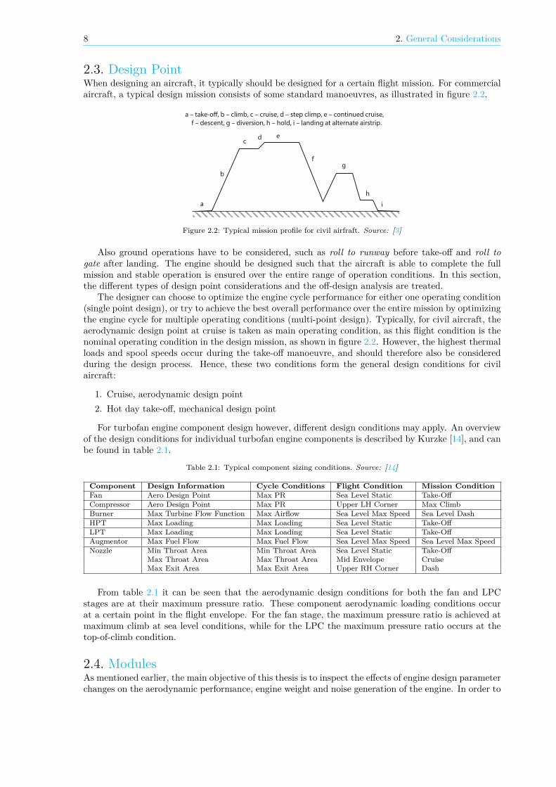
2.3. Design PointWhen designing an aircraft, it typically should be designed for a certain flight mission. For commercialaircraft, a typical design mission consists of some standard manoeuvres, as illustrated in figure 2.2.
a – take-o, b – climb, c – cruise, d – step climp, e – continued cruise,
f – descent, g – diversion, h – hold, i – landing at alternate airstrip.
a
b
c d e
f g
h
i
Figure 2.2: Typical mission profile for civil airfraft. Source: [3]
Also ground operations have to be considered, such as roll to runway before take-off and roll togate after landing. The engine should be designed such that the aircraft is able to complete the fullmission and stable operation is ensured over the entire range of operation conditions. In this section,the different types of design point considerations and the off-design analysis are treated.
The designer can choose to optimize the engine cycle performance for either one operating condition(single point design), or try to achieve the best overall performance over the entire mission by optimizingthe engine cycle for multiple operating conditions (multi-point design). Typically, for civil aircraft, theaerodynamic design point at cruise is taken as main operating condition, as this flight condition is thenominal operating condition in the design mission, as shown in figure 2.2. However, the highest thermalloads and spool speeds occur during the take-off manoeuvre, and should therefore also be consideredduring the design process. Hence, these two conditions form the general design conditions for civilaircraft:
1. Cruise, aerodynamic design point2. Hot day take-off, mechanical design point
For turbofan engine component design however, different design conditions may apply. An overviewof the design conditions for individual turbofan engine components is described by Kurzke [14], and canbe found in table 2.1.
Table 2.1: Typical component sizing conditions. Source: [14]
Component Design Information Cycle Conditions Flight Condition Mission ConditionFan Aero Design Point Max PR Sea Level Static Take-OffCompressor Aero Design Point Max PR Upper LH Corner Max ClimbBurner Max Turbine Flow Function Max Airflow Sea Level Max Speed Sea Level DashHPT Max Loading Max Loading Sea Level Static Take-OffLPT Max Loading Max Loading Sea Level Static Take-OffAugmentor Max Fuel Flow Max Fuel Flow Sea Level Max Speed Sea Level Max SpeedNozzle Min Throat Area Min Throat Area Sea Level Static Take-Off
Max Throat Area Max Throat Area Mid Envelope CruiseMax Exit Area Max Exit Area Upper RH Corner Dash
From table 2.1 it can be seen that the aerodynamic design conditions for both the fan and LPCstages are at their maximum pressure ratio. These component aerodynamic loading conditions occurat a certain point in the flight envelope. For the fan stage, the maximum pressure ratio is achieved atmaximum climb at sea level conditions, while for the LPC the maximum pressure ratio occurs at thetop-of-climb condition.
2.4. ModulesAs mentioned earlier, the main objective of this thesis is to inspect the effects of engine design parameterchanges on the aerodynamic performance, engine weight and noise generation of the engine. In order to
2.4. Modules 9
obtain these results, the performance of the engine is calculated using three modules: an aerodynamicsmodule, weight module and noise module.
2.4.1. Aerothermodynamic performanceThe aerodynamics module is used for the aero- and thermodynamic calculations in the fan and LPCstages. In the design process of both stages, many variables are not known on beforehand, while they arerequired for proper calculation of the gaspath analysis. Therefore, these parameters should be guessedinitially, and after calculating the gaspath the parameters are compared to the new calculated values.This routine is then repeated until the the guessed and calculated values have converged. Iterativesolver structures like this are used to ensure convergence of several design parameters in the fan andLPC desing case. A more detailed description of the solver structure for the fan and LPC stage aredescribed in sections 3.4.1 and 3.5.1 respectively.
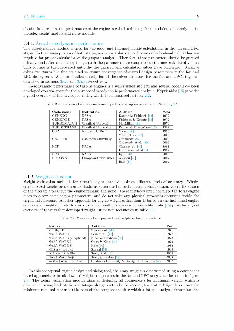
Aerodynamic performance of turbine engines is a well-studied subject, and several codes have beendeveloped over the years for the purpose of aerodynamic performance analysis. Kyprianidis [15] providesa good overview of the developed codes, which is summarized in table 2.2.
Table 2.2: Overview of aerothermodynamic performance optimisation codes. Source: [15]
Code name Institution Authors YearGENENG NASA Koenig & Fishbach [32] 1972GENENG II NASA Fishbach & Koenig [33] 1972TURBOMATCH Cranfield University MacMillan [34] 1974TURBOTRANS Cranfield University Palmer & Cheng-Zong [35] 1982GSP NLR & TU Delft Visser [36] 1995
Visser et al. [37] 2000GeSTPAn Chalmers University Grönstedt [38] 2000
Grönstedt et al. [39] 2002NCP NASA Claus et al. [40] 1991
Drummond et al. [41] 1992NPSS NASA Lylte [42] 2000PROOSIS European Universities Alexiou [43] 2007
Bala [44] 2007
2.4.2. Weight estimationWeight estimation methods for aircraft engines are available at different levels of accuracy. Whole-engine based weight prediction methods are often used in preliminary aircraft design, where the designof the aircraft alters, but the engine remains the same. These methods often correlate the total enginemass to a few basic engine parameters, and do not take any physical processes occurring inside theengine into account. Another approach for engine weight estimations is based on the individual enginecomponent weights for which also a variety of methods are readily available. Lolis [45] provides a goodoverview of these earlier developed weight estimation techniques in table 2.3.
Table 2.3: Overview of component based weight estimation methods.
Method Authors YearVTOL/STOL Sagerser al. [46] 1971NASA WATE Pera et al. [47] 1977NASA WATE (simplified) Klees & Fishbach [48] 1978NASA WATE-2 Onat & Klees [49] 1979NASA WATE-S Hale [50] 1982Military turbojet Sanghi [51] 1998Disk weight & life Tong et al. [11] 2004NASA WATE++ Tong & Naylow [52] 2008WeiCo (Weight & Cost) Chalmers University & Stuttgart University [53] 2007
In this conceptual engine design and sizing tool, the stage weight is determined using a componentbased approach. A break-down of weight components in the fan and LPC stages can be found in figure2.3. The weight estimation module aims at designing all components for minimum weight, which isdetermined using both static and fatigue design methods. In general, the static design determines theminimum required material thickness of the component, after which a fatigue analysis determines the

10 2. General Considerations
Total weight
Fan LPC Misc
blades
disks
casing
pressureblade containment
blades
disks
casing
nose cone
shaft
Figure 2.3: Engine weight component break-down.
fatigue design safety factor of the component. If the current fatigue safety factor does not meet thedesired safety factor, the material thickness is modified accordingly, and the process is repeated untilthe solution has converged.
2.4.3. Noise predictionNoise propagates from different sources of the engine, and there are large differences in the magnitudeof each of these sources between different engine types. Figure 2.4 shows a comparison of the magnitudeand sources of noise for both a low BPR and a high BPR turbofan engine. For bypass ratios largerthan 5, the increased internal noise sources dominate the jet noise.
Figure 2.4: Comparison of noise sources and magnitudes for low- and high-BPR turbofan engines. Source: [4]
A European research project called “Environmentally Friendly Aero Engines” (VITAL), also focuseson the development of an engine design tool, capable of evaluating new engine architectures in thepreliminary design phase. Within this research project, a Technoeconomic, Environmental and RiskAssessment tool called TERA2020 is being developed [16]. The tool consists of five modules: a noisemodule, an emissions module, a weight and dimensions module, an aircraft module and a performancemodule. The noise module is based on the extensive empirical acoustic prediction software called

2.5. Validation 11
Soprano. Kyprianidis et al. [16] give an overview of the implemented noise prediction methods used inthe Soprano code, which are shown in table 2.4 below.
Table 2.4: Overview of implemented noise prediction methods in Soprano. Source: [16]
Noise source Prediction methodFan and compressors Heidmann [54]
Kontos [55]Coaxial exhaust jet Stone & Krejsa [56]
SAE ARP 876D [57]Turbine Krejsa [58]Airframe Fink [59]Noise propagation SAE ARP 866A [60]
Chien & Soroka [61]SAE AIR 1751 [62]
Installation effects on jet noise Blackner and Bhat [63]Contra-rotating rotors Hanson modified ([64] and [65])interaction tone noise Heidmann adapted ([54] and [55])
The noise prediction methods in Soprano use the ANOPP method by Heidmann [54] and the im-proved ANOPP method by Kontos [55] for the fan and compressor noise estimation. Diéz [5] introduceda third noise estimation method from the Engineering Society of Data Units (ESDU), and did a com-parison with the three noise estimation techniques. It was concluded that no large differences betweenthe methods were appreciated.
2.5. ValidationThe separate modules are validated using existing engine data. For the CFM56-7B engine much datais available online. Test results from an engine testrun with a CFM56-7B24 engine are also availableand hence the engine is used for aerodynamics and weight module validation. For the noise modulevalidation, the CF6-80C2/B6F engine is used as extensive fan noise test were conducted with this engineof which the data is available.
For the noise module validation, the interaction with the aircraft is important, as this determinesthe flightpath and hence other values for the EPNL are observer. The CF6-80C2 is a high bypass ratioturbofan engine, manufactured by GE aviation which has been certified on several long-range aircraft,including the Airbus A300 and A310 series, Boeing’s 747-400 and 767 models and the McDonell DouglasMD-11. The CF6-80C2 engine is shown in figure 2.5. The CFM56-7B egine is shown in figure 2.6 somebasic engine characteristics are mentioned in table 2.5.
Figure 2.5: CF6-80C2 engine. Source: GE Aviation Figure 2.6: CFM56-7B engine. Source: CFMInternational

12 2. General Considerations
Table 2.5: Characteristic data for validation engines CF6-80C2/B6 (Roux [17]) and CFM56-7B24 (engine testrun data).
Parameter Symbol Engine UnitsCF6-80C2/B6 CFM56-7B24Stages fan/LPC/HPC 1 / 4 / 14 1 / 3 / 9Fan diameter 𝐷 2.362 1.5494 𝑚Length 𝐿 4.087 2.511 𝑚Mass 𝑚 4386 2366 𝑘𝑔Bypass ratio 𝐵𝑃𝑅 5.06 5.06 −Overall pressure ratio 𝑂𝑃𝑅 31.1 25.383 −Take-off thrust 𝑇 267200 104570 𝑁Mass flow rate − 342.9Specific fuel consumption 𝑆𝐹𝐶 9.5 ⋅ 10 1.1061 ⋅ 10 ⋅

3Aerodynamics
3.1. Governing equations and assumptionsFor the flowfield analysis through the axial fan and compressor components, the Navier-Stokes equationsare used as a starting point. However, as many turbine engine design handbooks suggest, for the purposeof the conceptual design phase some simplifying assumptions can be made with respect to the flowfield:
• Steady flow, no variation of flowfield parameters in time, = 0
• Axisymmetric flow, no variation of flowfield parameters in tangent direction, = 0
• Adiabatic flow, no heat transfer between the flow and the walls, = 0
• Radial equilibrium, no radial shift of the stream surface outside the blade rows, 𝐶 = 0
Applying these assumptions to the set of Navier-Stokes equations greatly simplifies the three-dimensionalgaspath analysis. This leads to a set of governing equations which describe the compressible flow throughthe axial compressor and fan stage in this thesis, which are given below:
• Continuity equationThe continuity equation states that the total mass flow should be conserved in a given controlvolume. For compressible flow, the mass continuity is described by equation (3.1).
𝜌 𝐴 𝐶 = 𝜌 𝐴 𝐶 (3.1)
• Euler equationThe Euler’s turbine equation describes the fundamental working principle for turbomachinery, andrelates the temperature difference across a given control volume to the change in rotational speedand momentum. Equation (3.2) shows the equilibrium and the specific work or power consumedby the compressor.
𝑃 = = 𝑐 (𝑇 , − 𝑇 , ) = Ω(𝑟 𝐶 , − 𝑟 𝐶 , ) (3.2)
• Radial equilibrium equationThe full radial equilibrium equation is given by equation (3.3).
𝑐 𝜕𝑇𝜕𝑟 = 𝑇𝜕𝑠𝜕𝑟 + 𝐶
𝜕𝐶𝜕𝑟 + 𝐶𝑟 + 𝐶 𝜕𝐶
𝜕𝑟 − 𝐶 𝜕𝐶𝜕𝑧 (3.3)
The last term in the radial equilibrium equation accounts for the radial accelerations in theflowfield, which according to the earlier stated assumptions equals zero and hence is neglected.
The radial equilibrium equation is only applied at the fan stage. For rotating machinery with relativelysmall blade heights, such as the low pressure compressor, radial variations of the flowfield are relativelysmall, and these effects are assumed to be negligible. For the turbofan fan stage however, blades heights
13

14 3. Aerodynamics
are typically too large to ignore the variation of the flowfield along the blade span, and hence radialequilibrium should be applied to ensure a feasible design output.
Some general equations used for determining the change in total air properties and related staticproperties are discussed here as well. First, the total temperature ratio over an arbitrary stage is forthree cases: the ideal case, assuming constant isentropic efficiency and assuming constant polytropicefficiency.
𝑇 ,𝑇 ,
= (𝑝 ,𝑝 ,) Ideal case (3.4)
= 1 + 1𝜂 ((𝑝 ,𝑝 ,
) − 1) Isentropic efficiency (3.5)
= (𝑝 ,𝑝 ,)
Polytropic efficiency (3.6)
If the total conditions of the airflow are known, the static properties can be derived using equations(3.7) and (3.8):
𝑇 = 𝑇 , ⋅ (1 +𝜅 − 12 ⋅ 𝑀 ) = 𝑇 , −
𝑉2 ⋅ 𝑐 ,
(3.7)
𝑝 = 𝑝 , ⋅ (1 +𝜅 − 12 ⋅ 𝑀 ) (3.8)
3.2. Non-dimensional performance parametersIn compressor design it is common practice for a designer to control three main criteria: the flowcapacity, the work done per stage and the distribution of flow diffusion over the rotor and stator bladerow. These three specifications are controlled by non-dimensionalized performance parameters, to makethem representative to any given operative condition.
Stage flow coefficientThe flow coefficient controls the flow capacity, and is defined as the axial flow velocity non-dimensionalizedby the rotational velocity, as shown in equation (3.9).
𝜙 = 𝐶𝑈 (3.9)
Stage loading coefficientThe dimensionless work done in a stage is expressed by the stage loading coefficient, which is derivedfrom Euler’s equation (3.2) and non-dimensionalized using the rotational velocity.
𝜓 = Δℎ𝑈 = 𝐶 , − 𝐶 ,
𝑈 (3.10)
Stage reactionThe distribution of diffusion between rotor and stator blade rows is given by the stage reaction. Thedefinition of the stage reaction is the ratio of the rotor static enthalpy rise divided by the stage totalenthalpy rise.
Λ = ℎ − ℎℎ − ℎ (3.11)

3.2. Non-dimensional performance parameters 15
For repeating stage designs (𝐶 = 𝐶 ), the stage reaction can be rewritten in the following forms
Λ = 𝑊 , +𝑊 ,2𝑈 = 𝜙(tan𝛽 + tan𝛽 )
2 (3.12)
Λ = 1 + 𝜙(tan𝛽 + tan𝛼 )2 (3.13)
Apart from the above mentioned design parameters, there are some non-dimensional performanceparameters that describe the aerodynamic performance of the compressor stages.
EfficiencyThe total-to-total adiabatic stage efficiency is given by equation (3.14) and relates the stage totalpressure rise to the temperature rise of the stage. It defines the efficiency of the compression processby of the rotor and stator blade rows together.
𝜂 =,,
− 1,,− 1
(3.14)
Pressure- and temperature ratioThe stage total pressure ratio, Π, and total temperature ratio, 𝜏, are defined by equations (3.15) and(3.16) respectively.
Π = 𝑝 ,𝑝 ,
(3.15)
𝜏 = 𝑇 ,𝑇 ,
(3.16)
Axial- and rotational velocity ratioThe axial velocity ratio, 𝜇, defines the relative change in axial velocity over the blade row. Similarly,the rotational velocity ratio, 𝜈, gives the change in rotational velocity due to radial shift over the rotorblade. Axial- and rotational velocity ratios are described by equations (3.17) and (3.18) respectively.
𝜇 = 𝐶 ,𝐶 ,
(3.17)
𝜈 = 𝑈𝑈 (3.18)
DeHaller numberThe DeHaller number is a measure of the diffusion in each blade row. Too much diffusion in a bladerow could cause flow separation leading to compressor stall or surge. Therefore, the DeHaller number islimited to minimum value of 0.72 for both the rotor and stator blade rows, which is an acceptable valuefor modern turbofan engines [66]. Equations (3.19) and (3.20) give the DeHaller number calculationand limits for rotor and stator stages respectively.
𝐷𝐻 = 𝑊𝑊 ≥ 0.72 (3.19)
𝐷𝐻 = 𝐶𝐶 ≥ 0.72 (3.20)

16 3. Aerodynamics
3.3. Gas path analysisAerodynamic performance prediction of axial compressors is often performed using a gaspath analysis.In a gaspath analysis the aerodynamic properties of the airflow throughout the component are calculatedat all intermediate stations. From the resulting gas properties before and after the component, the stageperformance parameters can be determined using equations mentioned in section 3.2.
3.3.1. Design methodsA gaspath analysis can be performed at different levels of accuracy. In the conceptual design phase,usually simple methods are used to increase the computational performance of the design tool. Amethod often used in conceptual design of turbomachinery is the mean-line design method. In a mean-line design, the flow is defined by the mean flow properties at each station. More information aboutthe mean-line design method is given in section 3.3.1.
Although mean-line design methods are sufficiently accurate for most low- and high pressure com-pressor and turbine stages, the effect of the underlying simplifying assumption becomes apparent whenstages with larger blade heights, such as the fan stage, are considered. Due to the increasing effectof three-dimensional flow phenomena that are not fully captured by the mean-line design method, theperformance predictions start to deviate from the actual component performance. To better deal withthree-dimensional flow effects, a blade-element design method (BEM) is used, which will be furtherelaborated upon in section 3.3.1.
Even more accurate results can be obtained by performing Computational Fluid Dynamics (CFD)analysis. In CFD analysis the flow path is discretized using a meshgrid with a finite volume around everynode point. However, properly setting up the flow field and performing the analysis is a computationallytime consuming process. Therefore, CFD analysis is mainly used for specific cases in later design stages,and is not further considered in this thesis.
Mean-line designThe mean-line analysis is a one-dimensional design method commonly used in conceptual engine design.Although the method uses an extremely simplified representation of the actual flow field, it allows thedesigner to quickly investigate effects on the performance of the component. Extensive research has beendone in the field of compressor loss predictions and their use in conceptual design applications. Section3.5 will further elaborate on the design methodology and loss prediction methods used in the mean-linedesign method. Combination of this rather simple design method with current loss prediction modelshas proven to deliver accurate results for performance prediction of modern compressor and turbinestages. [67]
Blade-element methodIn the previous sections all calculations of the flow field were limited to the one-dimensional domain.For the low-pressure compressor component, a one-dimensional flow analysis at the mean-line results ina sufficiently accurate performance prediction for the conceptual design stage. However, in the fan stagethe radial change of velocities in the flowfield result in appreciable spanwise variation of performance.Therefore, the one-dimensional mean-line design approach does not provide suffice here, and a blade-element method is used instead. In a blade-element method (BEM), the flow field is discretized in anumber of smaller sections. At each section, a one-dimensional design approach is used to calculatethe flow properties before and after the stage. Radial equilibrium and mass continuity are checked forall sections, and the axial velocity ratio is modified accordingly to converge the solution. The designprocess is described in more detail in section 3.4.1.
3.3.2. Annulus geometryThe first step in the design process of a component is determining the inlet and outlet annulus di-mensions. For the fan stage the cross sectional area at the rotor inlet is determined using the inletcalculations as described in section 3.4.2. The input to the inlet calculation procedure should eitherbe the inlet Mach number or airspeed. To fully describe the inlet geometry, one geometric parametershould be provided as input. The provided dimension can either be a fixed radial location (hub, mean,tip or root-mean squared (RMS) radius) or the non-dimensional hub-to-tip ratio (HTR). With the pro-vided dimension and the annulus area, other dimensions can be calculated. Equation (3.21) shows the
3.3. Gas path analysis 17
hub radius calculation for provided hub-to-tip ratio.
𝑟 = √ 𝐴𝜋(1 − 𝐻𝑇𝑅 ) (3.21)
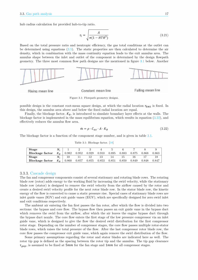
Based on the total pressure ratio and isentropic efficiency, the gas total conditions at the outlet canbe determined using equations (3.5). The static properties are then calculated to determine the airdensity, which in combination with the mass continuity equation leads to the exit annulus area. Theannulus shape between the inlet and outlet of the component is determined by the design flowpathgeometry. The three most common flow path designs are the mentioned in figure 3.1 below. Another
Figure 3.1: Flowpath geometry designs.
possible design is the constant root-mean square design, at which the radial location 𝑟 is fixed. Inthis design, the annulus area above and below the fixed radial location are equal.
Finally, the blockage factor, 𝐾 , is introduced to simulate boundary layer effects at the walls. Theblockage factor is implemented in the mass equilibrium equation, which results in equation (3.22), andeffectively reduces the annulus flow area.
= 𝜌 ⋅ 𝐶 ⋅ 𝐴 ⋅ 𝐾 (3.22)
The blockage factor is a function of the component stage number, and is given in table 3.1.
Table 3.1: Blockage factor. [18]
Stage 1 2 3 4 5 6 7 8 9Blockage factor 0.982 0.952 0.929 0.910 0.895 0.883 0.875 0.868 0.863Stage 10 11 12 13 14 15 16 17 18Blockage factor 0.860 0.857 0.855 0.853 0.851 0.850 0.849 0.848 0.847
3.3.3. Cascade designThe fan and compressor components consist of several stationary and rotating blade rows. The rotatingblade row (rotor) adds energy to the working fluid by increasing the swirl velocity, while the stationaryblade row (stator) is designed to remove the swirl velocity from the airflow caused by the rotor andcreate a desired swirl velocity profile for the next rotor blade row. In the stator blade row, the kineticenergy of the flow is converted to cause a static pressure rise. Special cases of stationary blade rows areinlet guide vanes (IGV) and exit guide vanes (EGV), which are specifically designed for zero swirl inletand exit conditions respectively.
The ambient air entering the fan first passes the fan rotor, after which the flow is divided into twosections: the bypass and core flow. The bypass flow then passes an exit guide vane in the bypass ductwhich removes the swirl from the airflow, after which the air leaves the engine bypass duct throughthe bypass duct nozzle. The core flow enters the first stage of the low pressure compressor via an inletguide vane, which is designed to give the flow the desired swirl distribution for the first compressorrotor stage. Depending on the number of compressor stages, the core flow passes multiple rotor-statorblade rows, which raises the total pressure of the flow. After the last compressor rotor blade row, thecore flow passes the compressor exit guide vane, which again remove the swirl distribution of the flow.
Some primary assumptions regarding the rotor and stator blades are indicated here as well. Therotor tip gap is defined as the spacing between the rotor tip and the annulus. The tip gap clearance𝜏 , is assumed to be fixed at 5𝑚𝑚 for the fan stage and 1𝑚𝑚 for all compressor stages.
18 3. Aerodynamics
NACA 65-seriesNACA 65-(24)10
Double-Circular-ArcDCA-𝜃(60)-𝑡/𝑐(10)-𝑟 (1)
British C.4 profile10C4/60C50
Figure 3.2: Three popular compressor cascades.
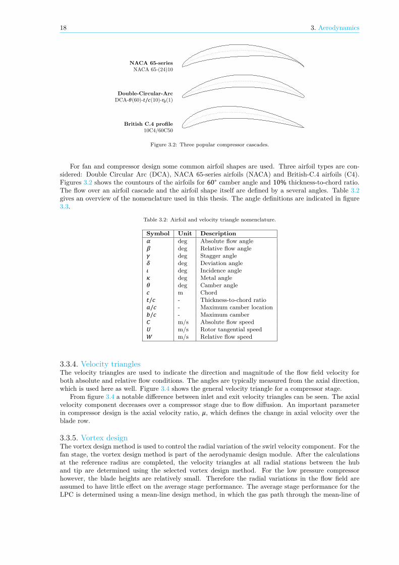
For fan and compressor design some common airfoil shapes are used. Three airfoil types are con-sidered: Double Circular Arc (DCA), NACA 65-series airfoils (NACA) and British-C.4 airfoils (C4).Figures 3.2 shows the countours of the airfoils for 60∘ camber angle and 10% thickness-to-chord ratio.The flow over an airfoil cascade and the airfoil shape itself are defined by a several angles. Table 3.2gives an overview of the nomenclature used in this thesis. The angle definitions are indicated in figure3.3.
Table 3.2: Airfoil and velocity triangle nomenclature.
Symbol Unit Descriptiondeg Absolute flow angledeg Relative flow angledeg Stagger angledeg Deviation angledeg Incidence angledeg Metal angledeg Camber anglem Chord
/ - Thickness-to-chord ratio/ - Maximum camber location/ - Maximum camber
m/s Absolute flow speedm/s Rotor tangential speedm/s Relative flow speed
3.3.4. Velocity trianglesThe velocity triangles are used to indicate the direction and magnitude of the flow field velocity forboth absolute and relative flow conditions. The angles are typically measured from the axial direction,which is used here as well. Figure 3.4 shows the general velocity triangle for a compressor stage.
From figure 3.4 a notable difference between inlet and exit velocity triangles can be seen. The axialvelocity component decreases over a compressor stage due to flow diffusion. An important parameterin compressor design is the axial velocity ratio, 𝜇, which defines the change in axial velocity over theblade row.
3.3.5. Vortex designThe vortex design method is used to control the radial variation of the swirl velocity component. For thefan stage, the vortex design method is part of the aerodynamic design module. After the calculationsat the reference radius are completed, the velocity triangles at all radial stations between the huband tip are determined using the selected vortex design method. For the low pressure compressorhowever, the blade heights are relatively small. Therefore the radial variations in the flow field areassumed to have little effect on the average stage performance. The average stage performance for theLPC is determined using a mean-line design method, in which the gas path through the mean-line of

3.3. Gas path analysis 19
κi
κi i
wi
wi i
chord
ι
δ
Figure 3.3: Fan blade angle nomenclature. Source: [5]
αi
ci
βi
wi
Ui
αii
cii
βiiwii
Uii
Figure 3.4: Velocity triangle nomenclature.Source: [5]
the component is considered to represent the average value in the compressor stage. It is a commonused method in preliminary compressor design, and is proven to provide sufficient accuracy for theperformance prediction in this design stage. A variety of blade vortex designs that are commonly usedin compressor design are discussed below.
Free vortex designThe free vortex design method is the most simple and well-known method. Using this method, the workis distributed evenly along the blade span. The stage reaction however increases with radius, and forshort compressor blades often results in highly twisted blade designs. The free vortex design method isdescribed by equation (3.23).
𝐶 = 𝑎𝑟 (3.23)
Forced vortex designThe forced vortex design is rarely used, due to the unfavourable effect of a quadratic increasing workcoefficient along the blade span. The governing equation for a forced vortex design is shown in equation(3.24).
𝐶 = 𝑎𝑟 (3.24)
Constant reaction designThe constant reaction whirl distribution ensures that the blade reaction and work coefficients are con-stant along the blade span. Although this is a favourable property of the whirl distribution, it is proneto result in high twist angles. The constant reaction vortex design is defined before and after the rotor,by equations (3.25) and (3.26) respectively.
𝐶 = 𝑎𝑟 − 𝑏𝑟 (3.25)
𝐶 = 𝑎𝑟 + 𝑏𝑟 (3.26)
Exponential vortex designIn comparison to the free vortex design, the exponential vortex design has an extra constant whichcauses a variation of the blade reaction with radius. The exponential vortex design method is describedbefore and after the rotor by equations (3.27) and (3.28) respectively.
𝐶 = 𝑎 − 𝑏𝑟 (3.27)

20 3. Aerodynamics
Table 3.3: Special cases for general vortex design.
Special caseExponential designConstant reaction designFree vortex designForced vortex design
𝐶 = 𝑎 + 𝑏𝑟 (3.28)
General vortex designThe general whirl distribution combines aspects of the free vortex design with an adjustable forcedvortex distribution. Equations (3.29) and (3.30) describe the tangent velocity distribution before andafter the rotor for the general vortex design respectively.
𝐶 = 𝑎𝑟 − 𝑏𝑟 (3.29)
𝐶 = 𝑎𝑟 + 𝑏𝑟 (3.30)
The vortex or swirl exponent, 𝑛, is used to control the shape of the radial whirl distribution. Table 3.3show special cases of the general whirl distribution that occur at specific combinations of 𝑛, 𝑎 and 𝑏.
3.3.6. Incidence angleThe incidence angle is defined as the difference between the inlet flow angle and the blade inlet metalangle. Several studies have shown that the cascade loss is dependent on the incidence angle, and at acertain angle, the optimum incidence angle, the cascade loss is minimal. Figure 3.5 shows the cascadeloss “bucket” and the optimum incidence angle location.
Figure 3.5: Optimum incidence angle and stall boundaries on the cascade loss curve. Source: [6]
There are several empirical methods available for optimum incidence angle calculations in cascadedesigns. To determine which method most accurately predicts the incidence angle in the consideredoperating conditions, five different methods are tested using experimental data available from rotormeasurements at the NASA Lewis Research Center. Table 3.4 shows the data that has been used forvalidation.
The three methods by Aungier [77], Howell [78] and Johnsen & Bullock [79] respectively, are inves-tigated here. Furthermore, Falck [8] presents in his work a set of equations, originally introduced byHoward, based on the original correlations from Johnsen & Bullock. Howard’s method is also includedin the analysis here.

3.3. Gas path analysis 21
Table 3.4: Experimental data used for validation of incidence angle and deviation angle prediction methods.
Designation Pressure ratio Tip-speed Mass flow Year Reference[ ] [ / ] [ / ]
Rotor 35 1.82 455 20.2 1978 [68]Rotor 36 1.82 455 20.2 1974 [69]Rotor 37 2.05 454 20.2 1980 [70]Rotor 51 1.15 243.8 29.9 1974 [71]Rotor 52 1.25 257.7 34.9 1974 [72]Rotor 53 1.35 302.8 32.7 1978 [73]Rotor 55 1.20 213.3 31.2 1974 [74]Rotor 57 1.38 289.6 29.6 1979 [75]Rotor 67 1.59 428.9 33.3 1979 [76]
The validation data from the NASA rotors mentioned in table 3.4 consists of geometrical data andmeasurements of flow angles, velocities at different turning speeds. For the comparison of methods, thedesign operating conditions are used, and the error is defined as the absolute difference between thepredicted and measured value. The combined results of the analysis are shown in figures 3.6 and 3.7.
Aungie
r
Howar
d
Howell
John
sen-
bullo
ck0
2
4
6
8
Abs
olut
e er
ror
[deg
] Mean errorRMS errorMax. error
Figure 3.6: Comparison of rotor incidence angle pre-diction methods using NASA rotor data (table 3.4).
Aungie
r
Howar
d
Howell
John
sen-
bullo
ck0
2
4
6
8
10
12A
bsol
ute
erro
r [d
eg] Mean error
RMS errorMax. error
Figure 3.7: Comparison of stator incidence angle pre-diction methods using NASA rotor data (table 3.4).
Although Howell predicts the incidence angle more accurately for the rotor, the other methods showapproximately the same results. The method that will be used to determine the minimum loss incidenceangle method is the method by Aungier, as it has been used in Tournier [67] and resulted in accuratepredictions when combined with the right deviation angle method, which is discussed next.
3.3.7. Deviation angleThe deviation angle is described by the difference between the trailing edge metal angle 𝜅 and therelative exit flow angle 𝛽 . Ideally the flow over the blade cascade would perfectly follow the contoursof the cascade such that no deviation angle would be present. However, due to pressure differencesbetween the upper and lower surface of the airfoil the airflow is unable to stay attached to the surfaceand flow deviation occurs. The deviation angle gives an indication of the pressure loss in a stage andseveral empirical methods are available to predict the deviation angle based on flow conditions andcascade geometry. A total number of 9 deviation angle prediction methods is considered, and a similarcomparison of techniques as for the incidence angle methods is performed here. The rotor data fromtable 3.4 is used here as well, and the results are shown in figures 3.8 and 3.9.
For both the rotor and stator, the deviation angle is best predicted using Johnsen and Bullock’smethod. This method, in combination with Aungier’s method for the incidence angle, has been usedin Tournier’s work for determining the blade metal angles corresponding to the minimum loss in com-pressor cascades. Since the combined performance of these two methods has proven to deliver accuratepredictions, these design methods are used here as well.
The iterative design methodology of determining the minimum loss blade metal angles based on theknown air flow angles is shown in a flow diagram in figure 3.10.

22 3. Aerodynamics
Boyce
Carte
r
John
sen-
Bulloc
k
Howell
-Sim
ple
Howell
-Impr
oved
Howell
-Mod
ified
Lieble
in
McK
enzie
Schob
eiri
0
2
4
6
8
10
Abs
olut
e er
ror
[deg
] Mean errorRMS errorMax. error
Figure 3.8: Comparison of rotor deviation angle pre-diction methods using NASA rotor data (table 3.4).
Boyce
Carte
r
John
sen-
Bulloc
k
Howell
-Sim
ple
Howell
-Impr
oved
Howell
-Mod
ified
Lieble
in
McK
enzie
Schob
eiri
0
5
10
Abs
olut
e er
ror
[deg
] Mean errorRMS errorMax. error
Figure 3.9: Comparison of stator deviation angle pre-diction methods using NASA rotor data (table 3.4).
input
initial guess𝛿 = 0
initial guess𝜄 = 0
blade profilecamberline
calculate blade metalangles: 𝜅 , 𝜅 , 𝜃, 𝜆
calculate 𝜄(Howell’s method)
|𝜄 − 𝜄 | ≤ 𝜀
calculate blademetal angles: 𝜃, 𝜆,𝑏/𝑐, 𝜒 , 𝜒 , 𝜅 , 𝜅
calculate 𝜄𝜄 = 𝛽 − 𝜅
|𝜄 − 𝜄 | ≤ 𝜀
calculate 𝛿(Johnsen and Bul-
lock’s method)
|𝛿 − 𝛿 | ≤ 𝜀
output
update𝜄
update𝜄
update𝛿
DCANACA
noyes
noyes
no
yes
Figure 3.10: Iterative solving method for blade angles.
3.3.8. Loss sourcesNow the flowfield over a cascade is properly defined, the analysis is extended to the three-dimensionaldomain. Complex flow fields develop inside the compressor stage due to the three-dimensional effectscaused by rotating hardware. These effects are difficult to model, however, these flow phenomena shouldbe taken into account to make a good estimate of the pressure loss in a compressor cascade. Figures3.12 and 3.12 show some of the typical effects that occur in a compressor stage.
The basic sources of loss occurring in the fan stage are primary losses, secondary losses and shocklosses. The primary losses are mainly caused by the blade profile, and capture the effects of momentum

3.4. Fan Analysis & Design 23
Figure 3.11: Development of tip, hub and endwall vorticesin fan rotor and stator blade channels. Source: [7]
Figure 3.12: Flow fields in a compressor cascade with losssources indicated. Source: [8]
loss over the blade, but also include losses resulting from induced drag. Secondary losses are causedby wall phenomena, such as the tip clearance, and are often referred to as endwall losses. Figure 3.11shows the development of tip and hub endwall vortices, causing the secondary losses. Shock loss occurwhen the accelerating flow over the suction side of the fan blade exceeds the sonic limit. Using a lossmodel originally proposed by Lieblein et al.[80], all of these losses are incorporated in one loss factor,𝑍, from which the isentropic efficiency can be determined directly. The calculation of the fan cascadeloss coefficient is explained in more detail in section 3.4.3.
In the LPC stage, the isentropic efficiency is determined by several loss models. Tournier & El-Genk [67] provide a well-documented summary of some of the latest loss models, and define the totalloss coefficient as the sum of five different loss sources. The losses that are captured in the total losscoefficient are: profile loss 𝑤 , secondary losses 𝑤 , end-wall friction loss 𝑤 , tip clearance losses𝑤 and shock losses 𝑤 . From the total loss coefficient 𝑤, the ratio stagnation pressure loss overthe dynamic inlet pressure can be calculated, and hence the total pressure loss in the stage can bedetermined. This method is elaborated upon in section 3.5.3.
3.4. Fan Analysis & DesignThe aerodynamic performance analysis and design of the fan stage is treated in this section. The fanstage of a typical high bypass ratio turbofan engine is indicated in figure 3.13. The main purposes ofthe fan stage is to accelerate the bypass air to generate thrust, and increase the pressure ratio for thecore inlet air. The fan stage consist of a rotor- and stator blade row. The rotor blade row is positionedin front of the engine, after which a splitter divides the airflow into a primary flow section, the coreflow, and a secondary flow section, the bypass stream. The bypass stream only passes a stator bladerow to remove the swirl velocity, which ideally produce an axial flowfield at the exit of the stator row.Then the air is expanded through the bypass nozzle generate a thrust force. The primary flow however,enters the low-pressure compressor stage via an inlet guide vane (IGV). It should be noted here that thestator vanes in the bypass duct are considered part of the fan design routine, while the IGV is designedusing the LPC design routine.
First the design methodology used for the fan stage is explained in section 3.4.1. After that, theseparate steps in the fan stage analysis and design process are treated, starting with the inlet calculationsin section 3.4.2, followed by efficiency calculations using loss prediction models as explained in section3.4.3.
3.4.1. Design methodologyThe gas path analysis is carried out using a Blade Element Method (BEM) as described in section3.3.1. The analysis of the fan stage consists of an iterative solving routine. Calculating the state afterthe rotor requires knowledge of the stage performance. However, as the stage performance is not yet
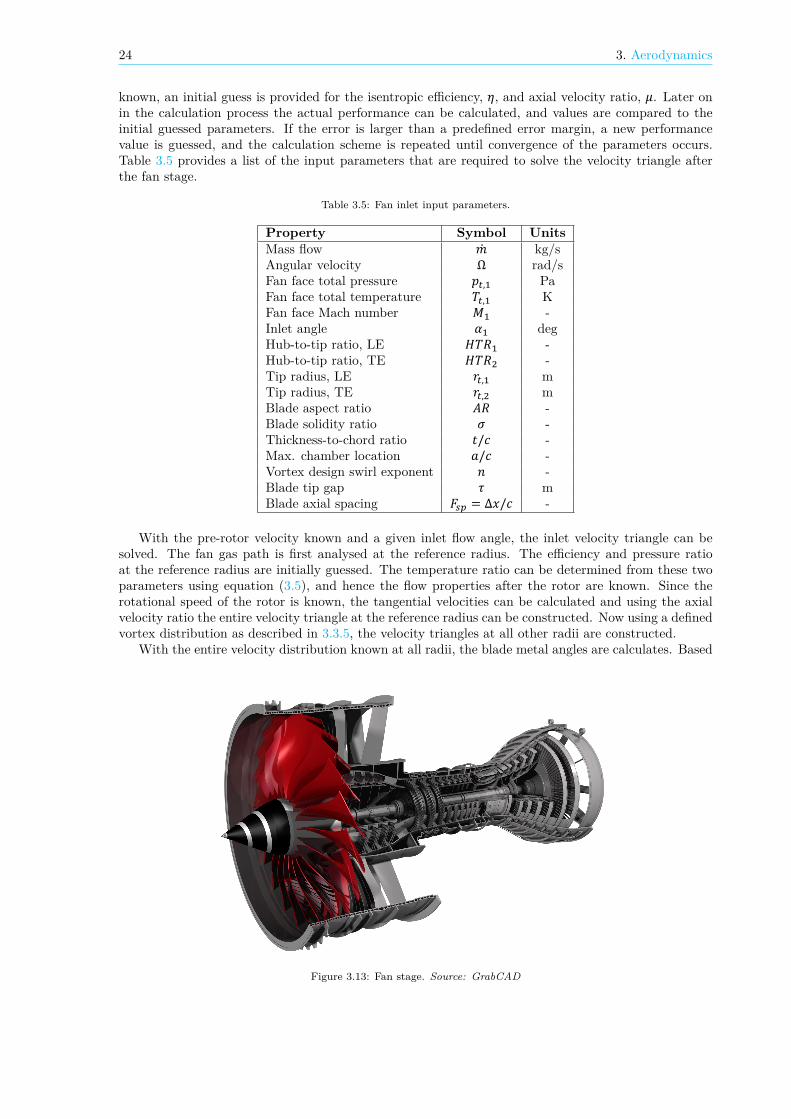
24 3. Aerodynamics
known, an initial guess is provided for the isentropic efficiency, 𝜂, and axial velocity ratio, 𝜇. Later onin the calculation process the actual performance can be calculated, and values are compared to theinitial guessed parameters. If the error is larger than a predefined error margin, a new performancevalue is guessed, and the calculation scheme is repeated until convergence of the parameters occurs.Table 3.5 provides a list of the input parameters that are required to solve the velocity triangle afterthe fan stage.
Table 3.5: Fan inlet input parameters.
Property Symbol UnitsMass flow kg/sAngular velocity Ω rad/sFan face total pressure 𝑝 , PaFan face total temperature 𝑇 , KFan face Mach number 𝑀 -Inlet angle 𝛼 degHub-to-tip ratio, LE 𝐻𝑇𝑅 -Hub-to-tip ratio, TE 𝐻𝑇𝑅 -Tip radius, LE 𝑟 , mTip radius, TE 𝑟 , mBlade aspect ratio 𝐴𝑅 -Blade solidity ratio 𝜎 -Thickness-to-chord ratio 𝑡/𝑐 -Max. chamber location 𝑎/𝑐 -Vortex design swirl exponent 𝑛 -Blade tip gap 𝜏 mBlade axial spacing 𝐹 = Δ𝑥/𝑐 -
With the pre-rotor velocity known and a given inlet flow angle, the inlet velocity triangle can besolved. The fan gas path is first analysed at the reference radius. The efficiency and pressure ratioat the reference radius are initially guessed. The temperature ratio can be determined from these twoparameters using equation (3.5), and hence the flow properties after the rotor are known. Since therotational speed of the rotor is known, the tangential velocities can be calculated and using the axialvelocity ratio the entire velocity triangle at the reference radius can be constructed. Now using a definedvortex distribution as described in 3.3.5, the velocity triangles at all other radii are constructed.
With the entire velocity distribution known at all radii, the blade metal angles are calculates. Based
Figure 3.13: Fan stage. Source: GrabCAD

3.4. Fan Analysis & Design 25
on the minimum loss cascade design method shown in figure 3.10, the blade metal angles are calculated.With the blade geometry and the flow field known, the pressure loss can be determined using thepressure loss prediction method described in section 3.4.3.
Now all information is available to check if the guessed axial velocity ratio, 𝜇, is correct. Diézshowed that the a simple check using the continuity equation alone is not sufficient [5]. Hence, theradial equilibrium equation (3.3) is applied with the radial acceleration term neglected. As explainedearlier, this results in a partial differential equation (PDE) which can then be rewritten in the form ofan ordinary differential equation (ODE). The resulting ODE can be solved for the exit axial velocityterm by applying the trapezoidal rule, resulting in equation (3.31)
𝐶 , = √𝐶𝐹 ⋅ (𝐹 + 𝐹 − 𝐹 − 𝐹 − 𝐹 ) (3.31)
Where the constants 𝐶𝐹 and 𝐹 are given by equations (3.32) to (3.37) respectively.
𝐶𝐹 = 1
1− ln⎡⎢⎢⎣
(,
)
(,
)
⎤⎥⎥⎦
(3.32)
𝐹 = 𝐶 , , (1+𝜅 − 12𝜅 ln[
( , )( , )
]) (3.33)
𝐹 = 2𝑐 (𝑇 − 𝑇 , ) (3.34)𝐹 = (𝐶 − 𝐶 , ) (3.35)
𝐹 = (𝐶𝑟 −𝐶 ,𝑟 ) (𝑟 − 𝑟 ) (3.36)
𝐹 = ln [( , )( , )
] [𝑅(𝑇 + 𝑇 , ) − 𝜅 − 12𝜅 (𝐶 + 𝐶 , )] (3.37)
Performance parameters such as pressure ratio, temperature ratio, and isentropic efficiency perradial section are then calculated. The weighted average of these performance parameters is used todetermine the stage performance for the core and bypass sections of the fan blade, which are comparedto their desired values after which the design input is altered accordingly. This process is repeated untilthe desired and calculated performance parameters converged.
3.4.2. Inlet calculationsThe input to the fan design calculation process consists of the static air properties of the ambient, 𝑝and 𝑇 , the mass flow ingestion , and the airspeed, either expressed by the axial Mach number, 𝑀 ,or the axial velocity, 𝐶 . Assuming a fixed isentropic efficiency of the inlet, the total temperature andpressure at the fan rotor leading edge can be determined using equations (3.38) and (3.40) respectively.
𝑇 , = 𝑇 + 𝐶2𝑐 (3.38)
= 𝑇 (1 + 𝜅 − 12 𝑀 ) (3.39)
𝑝 , = 𝑝 (1 + 𝜂 ,𝐶2𝑐 𝑇 ) (3.40)
= 𝑝 (1 + 𝜂 ,𝜅 − 12 𝑀 ) (3.41)
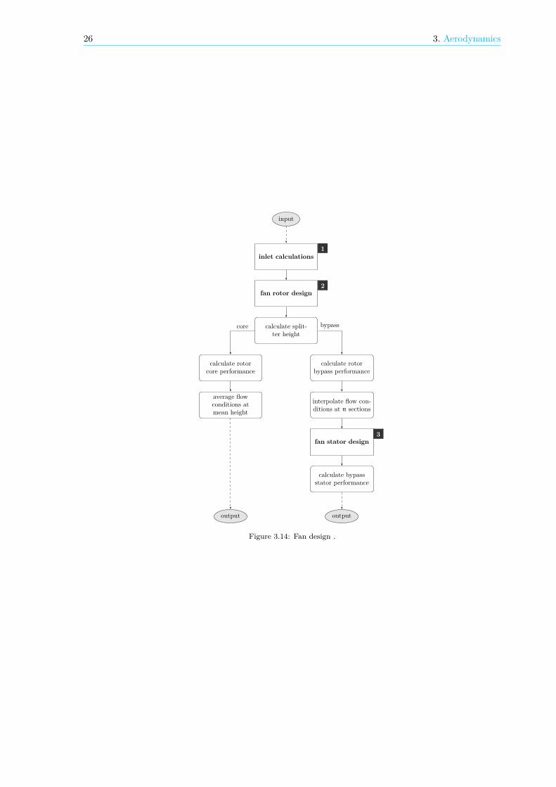
26 3. Aerodynamics
input
inlet calculations1
fan rotor design2
calculate split-ter height
calculate rotorcore performance
calculate rotorbypass performance
interpolate flow con-ditions at 𝑛 sections
fan stator design3
calculate bypassstator performance
outputoutput
average flowconditions atmean height
core bypass
Figure 3.14: Fan design .

3.4. Fan Analysis & Design 27
input
guessΠ
guess𝜇
guess𝜂
solve atreference radius
|𝜂 − 𝜂 , | ≤ 𝜀
vortex design
solve atother radii
check radialequilibrium
|𝐶 − 𝐶 , | ≤ 𝜀
check mass flowequilibrium
| − | ≤ 𝜀
|Π − Π| ≤ 𝜀
output
update𝜂
shape𝜇
scale𝜇
updateΠ
no
yes
no
yes
no
yes
no
yes
Figure 3.15: Iterative solving method for fan rotor design.
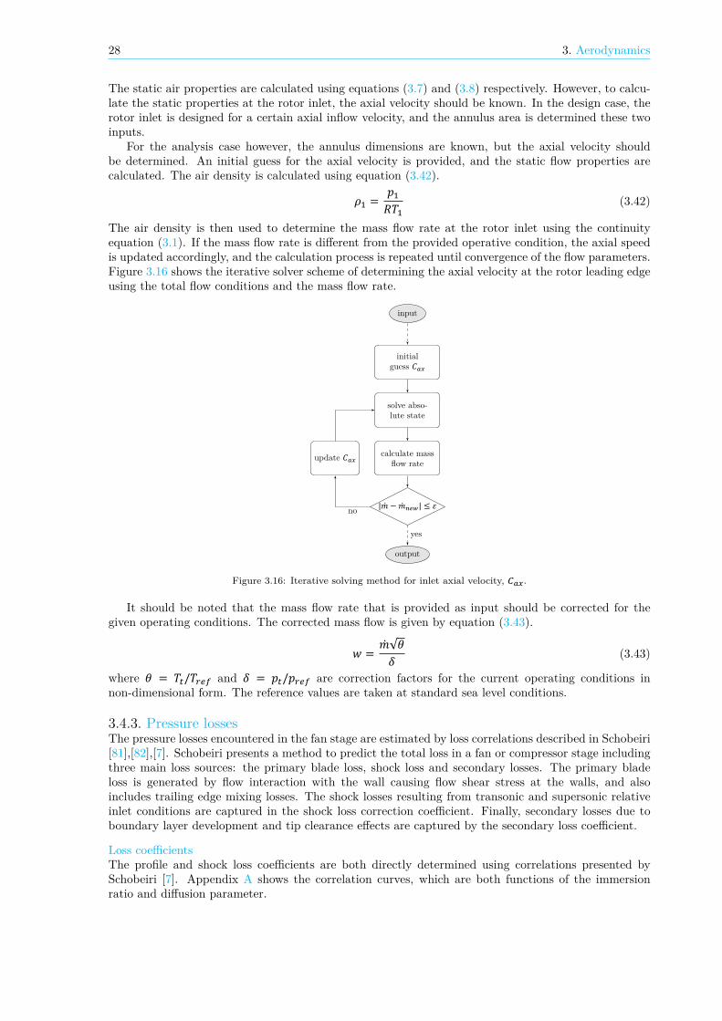
28 3. Aerodynamics
The static air properties are calculated using equations (3.7) and (3.8) respectively. However, to calcu-late the static properties at the rotor inlet, the axial velocity should be known. In the design case, therotor inlet is designed for a certain axial inflow velocity, and the annulus area is determined these twoinputs.
For the analysis case however, the annulus dimensions are known, but the axial velocity shouldbe determined. An initial guess for the axial velocity is provided, and the static flow properties arecalculated. The air density is calculated using equation (3.42).
𝜌 = 𝑝𝑅𝑇 (3.42)
The air density is then used to determine the mass flow rate at the rotor inlet using the continuityequation (3.1). If the mass flow rate is different from the provided operative condition, the axial speedis updated accordingly, and the calculation process is repeated until convergence of the flow parameters.Figure 3.16 shows the iterative solver scheme of determining the axial velocity at the rotor leading edgeusing the total flow conditions and the mass flow rate.
input
initialguess 𝐶
solve abso-lute state
calculate massflow rateupdate 𝐶
| − | ≤ 𝜀
output
no
yes
Figure 3.16: Iterative solving method for inlet axial velocity, .
It should be noted that the mass flow rate that is provided as input should be corrected for thegiven operating conditions. The corrected mass flow is given by equation (3.43).
𝑤 = √𝜃𝛿 (3.43)
where 𝜃 = 𝑇 /𝑇 and 𝛿 = 𝑝 /𝑝 are correction factors for the current operating conditions innon-dimensional form. The reference values are taken at standard sea level conditions.
3.4.3. Pressure lossesThe pressure losses encountered in the fan stage are estimated by loss correlations described in Schobeiri[81],[82],[7]. Schobeiri presents a method to predict the total loss in a fan or compressor stage includingthree main loss sources: the primary blade loss, shock loss and secondary losses. The primary bladeloss is generated by flow interaction with the wall causing flow shear stress at the walls, and alsoincludes trailing edge mixing losses. The shock losses resulting from transonic and supersonic relativeinlet conditions are captured in the shock loss correction coefficient. Finally, secondary losses due toboundary layer development and tip clearance effects are captured by the secondary loss coefficient.
Loss coefficientsThe profile and shock loss coefficients are both directly determined using correlations presented bySchobeiri [7]. Appendix A shows the correlation curves, which are both functions of the immersionratio and diffusion parameter.

3.4. Fan Analysis & Design 29
The immersion ratio, 𝐻, is the relative radial position from the blade tip as a function of the bladeheight. Hence, the immersion ratio is written as equation (3.44).
𝐻 = 𝑟 − 𝑟𝑟 − 𝑟 (3.44)
The flow diffusion is calculated using the modified diffusion parameter, 𝐷 , as suggested by Schobeiri.The modified diffusion parameters takes the compressibility effects into account, and using the describedangle definitions from figure 3.3, diffusion parameter is given by equation (3.45).
𝐷 = 1 − 𝜇 cos𝛽cos𝛽 + 𝜈 cos𝛽
𝜎(𝜈 + 1) [𝜇𝜈𝜙(1 − 𝜈 ) + tan𝛽 − tan𝛽 ] × [1 − 𝜇 cos𝛽
cos𝛽 𝑀 (𝜇 cos𝛽cos𝛽 − 1)]
(3.45)
Although the loss coefficients are determined from the correlation data, it is important to address thederivation of the profile loss coefficient here. The profile loss coefficient is defined as a function of therelative flow angles, 𝛽 and 𝛽 , blade solidity ratio, 𝜎 and the boundary layer momentum thickness, ,as shown in equation (3.46).
𝜁 = 𝜎𝛿𝑐 (sin𝛽sin𝛽 ) ⋅ 𝐹(𝐻 ,𝐻 , 𝛿𝑐 , 𝜎) (3.46)
where the function 𝐹 is a function of the above described parameters and the displacement and energyform factors, 𝐻12 and 𝐻32 respectively.
Correction factorsAll correlations are based on experimental results with specific blade geometries and flow conditions.By making use of correction factors for Mach number, Reynolds number and blade thickness, thesecorrelations can be applied to other flow conditions as well.
The Mach number correction should be applied when the Mach number locally reaches values of 𝑀 ≥1.0. Jansen and Moffatt [83] suggested that the total pressure loss increases rapidly after the maximumlocal flow velocity reaches values above a critical Mach number. The critical Mach number is given byequation (3.47).
(𝑉𝑉 ) − 1 =1 − ( + 𝑀 , )
−1 + (1 + 𝑀 , )(3.47)
Davis [84] suggested a relation to directly determine the critical Mach from the maximum velocity ratio.The relation is given in equation (3.48) below.
𝑀 , = 2.925 − 2.948(𝑉𝑉 ) + 1.17(𝑉𝑉 ) − 0.1614(𝑉𝑉 ) (3.48)
Now the profile loss coefficient is corrected using the critical Mach number by applying equation (3.49).
𝜁 , = 𝜁 (𝐴(𝑀 −𝑀 , ) + 1.0) (3.49)
with 𝐴 = 1.8 − 2.0 [85].
For pressure loss calculations at lower Reynolds numbers, the profile loss should be corrected accordingly.The profile loss correction applies only to a range of Reynolds number 𝑅𝑒 < 2.5 ⋅ 10 . The correctionfactor is given by equation (3.50).
𝜁 , = 𝜁 ( 𝑅𝑒2.5 ⋅ 10 )
.(3.50)
At last, the blade thickness effect is considered by correcting the profile loss accordingly. A relationbetween the blade thickness and boundary layer momentum thickness is provided in Schobeiri [7].
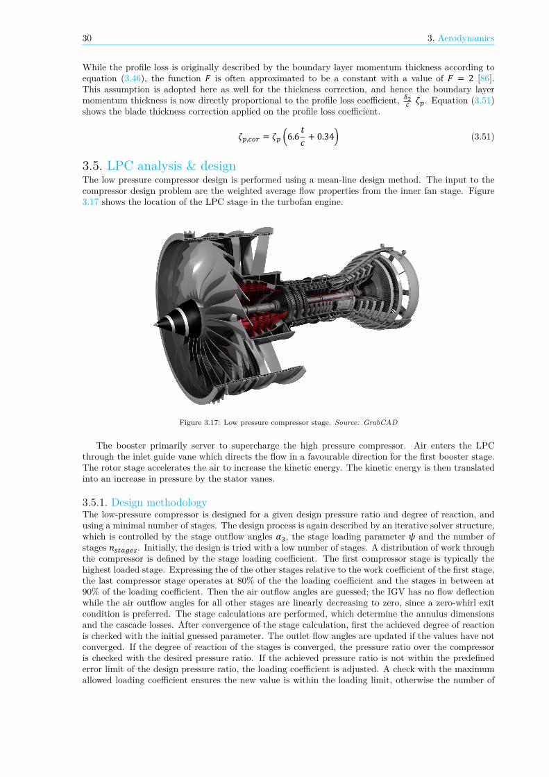
30 3. Aerodynamics
While the profile loss is originally described by the boundary layer momentum thickness according toequation (3.46), the function 𝐹 is often approximated to be a constant with a value of 𝐹 = 2 [86].This assumption is adopted here as well for the thickness correction, and hence the boundary layermomentum thickness is now directly proportional to the profile loss coefficient, 𝜁 . Equation (3.51)shows the blade thickness correction applied on the profile loss coefficient.
𝜁 , = 𝜁 (6.6 𝑡𝑐 + 0.34) (3.51)
3.5. LPC analysis & designThe low pressure compressor design is performed using a mean-line design method. The input to thecompressor design problem are the weighted average flow properties from the inner fan stage. Figure3.17 shows the location of the LPC stage in the turbofan engine.
Figure 3.17: Low pressure compressor stage. Source: GrabCAD
The booster primarily server to supercharge the high pressure compressor. Air enters the LPCthrough the inlet guide vane which directs the flow in a favourable direction for the first booster stage.The rotor stage accelerates the air to increase the kinetic energy. The kinetic energy is then translatedinto an increase in pressure by the stator vanes.
3.5.1. Design methodologyThe low-pressure compressor is designed for a given design pressure ratio and degree of reaction, andusing a minimal number of stages. The design process is again described by an iterative solver structure,which is controlled by the stage outflow angles 𝛼 , the stage loading parameter 𝜓 and the number ofstages 𝑛 . Initially, the design is tried with a low number of stages. A distribution of work throughthe compressor is defined by the stage loading coefficient. The first compressor stage is typically thehighest loaded stage. Expressing the of the other stages relative to the work coefficient of the first stage,the last compressor stage operates at 80% of the the loading coefficient and the stages in between at90% of the loading coefficient. Then the air outflow angles are guessed; the IGV has no flow deflectionwhile the air outflow angles for all other stages are linearly decreasing to zero, since a zero-whirl exitcondition is preferred. The stage calculations are performed, which determine the annulus dimensionsand the cascade losses. After convergence of the stage calculation, first the achieved degree of reactionis checked with the initial guessed parameter. The outlet flow angles are updated if the values have notconverged. If the degree of reaction of the stages is converged, the pressure ratio over the compressoris checked with the desired pressure ratio. If the achieved pressure ratio is not within the predefinederror limit of the design pressure ratio, the loading coefficient is adjusted. A check with the maximumallowed loading coefficient ensures the new value is within the loading limit, otherwise the number of
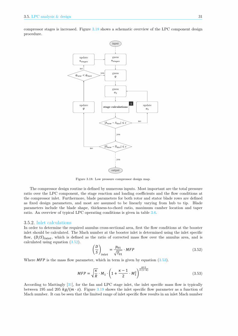
3.5. LPC analysis & design 31
compressor stages is increased. Figure 3.18 shows a schematic overview of the LPC component designprocedure.
input
guess𝑛
guess𝜓
guess𝛼
stage calculations1
|Λ − Λ | ≤ 𝜀
|Π − Π | ≤ 𝜀
output
update𝛼
update𝜓
𝜓 < 𝜓
update𝑛
no
yes
no
yes
noyes
Figure 3.18: Low pressure compressor design map.
The compressor design routine is defined by numerous inputs. Most important are the total pressureratio over the LPC component, the stage reaction and loading coefficients and the flow conditions atthe compressor inlet. Furthermore, blade parameters for both rotor and stator blade rows are definedas fixed design parameters, and most are assumed to be linearly varying from hub to tip. Bladeparameters include the blade shape, thickness-to-chord ratio, maximum camber location and taperratio. An overview of typical LPC operating conditions is given in table 3.6.
3.5.2. Inlet calculationsIn order to determine the required annulus cross-sectional area, first the flow conditions at the boosterinlet should be calculated. The Mach number at the booster inlet is determined using the inlet specificflow, (𝐷/𝑆) , which is defined as the ratio of corrected mass flow over the annulus area, and iscalculated using equation (3.52).
(𝐷𝑆 ) = 𝑝√𝑇
⋅ 𝑀𝐹𝑃 (3.52)
Where 𝑀𝐹𝑃 is the mass flow parameter, which in term is given by equation (3.53).
𝑀𝐹𝑃 = √𝜅𝑅 ⋅ 𝑀 ⋅ (1 + 𝜅 − 12 ⋅ 𝑀 )⋅( )
(3.53)
According to Mattingly [31], for the fan and LPC stage inlet, the inlet specific mass flow is typicallybetween 195 and 205 𝑘𝑔/(𝑚 ⋅ 𝑠). Figure 3.19 shows the inlet specific flow parameter as a function ofMach number. It can be seen that the limited range of inlet specific flow results in an inlet Mach number

32 3. Aerodynamics
Table 3.6: LPC inlet input parameters.
Property Symbol UnitsDesign pressure ratio 𝑃𝑅 -Number of stages 𝑛 -Mass flow kg/sAngular velocity Ω rad/sInlet total pressure 𝑝 , PaInlet total temperature 𝑇 , KInlet Mach number 𝑀 -Inlet flow angle 𝛼 degHub-to-tip ratio, LE 𝐻𝑇𝑅 -Tip radius, LE 𝑟 , mBlade aspect ratio 𝐴𝑅 -Blade solidity ratio 𝜎 -Thickness-to-chord ratio 𝑡/𝑐 -Max. chamber location 𝑎/𝑐 -Blade tip gap 𝜏 mBlade axial spacing 𝐹 = Δ𝑥/𝑐 -
0.2 0.3 0.4 0.5 0.6 0.7 0.8 0.9 1 1.1 1.2100
120
140
160
180
200
220
240
Mach number, M [-]
Inle
tsp
ecifi
cflo
w,(
D/S
)[k
g/s/
m2 ]
Figure 3.19: Inlet specific flow vs. Mach number with typical LPC inlet conditions indicated.

3.5. LPC analysis & design 33
range of 0.55 to 0.65 approximately. Using the mass flow parameter, the cross-sectional annulus areaat the LPC inlet can be calculated using equation (3.54):
𝐴 = ⋅ √𝑇𝑀𝐹𝑃 ⋅ 𝑝 ⋅ cos𝛼 = 𝜋 ⋅ (𝑟 , − 𝑟 , ) (3.54)
The hub-to-tip radius ratio, (𝑟 /𝑟 ), is an input parameter and is lower limited due to problems with theradial velocity distribution with low values for (𝑟 /𝑟 ). A typically used lower limit for the hub-to-tipratio is 0.4. [87] [31]
3.5.3. Pressure lossesThe LPC isentropic efficiency is determined by several loss models. Tournier & El-Genk [67] providean overview of empirical methods used to determine the losses in a compressor cascade based on fiveloss sources: profile loss 𝑤 , secondary losses 𝑤 , endwall friction losses 𝑤 , tip clearance losses𝑤 and shock losses 𝑤 . The total loss coefficient is then computed using equation (3.55).
𝑤 = 𝑤 +𝑤 +𝑤 +𝑤 +𝑤 (3.55)
From the total loss parameter 𝑤, the ratio of loss in stagnation pressure over the dynamic inlet pressurecan be calculated, using equation (3.56).
𝑤 = Δ𝑝𝑝 , − 𝑝
(3.56)
The computation of the five loss sources is treated separately in the following sections.
Profile lossThe blade profile pressure loss coefficient is described by Lieblein [88] as:
𝑤 = 2(𝜃𝑐 )𝜎
cos𝛽 (cos𝛽cos𝛽 ) ( 2𝐻
3𝐻 − 1) [1 − (𝜎𝑐 )
𝜎𝐻cos𝛽 ] (3.57)
Where 𝜃 is the momentum thickness of the boundary layer at the blade outlet, and in the dimensionlessform it is given as
𝜃𝑐 = (𝜃𝑐 ) ⋅ 𝜁 ⋅ 𝜁 ⋅ 𝜁 (3.58)
Furthermore, 𝐻 is the boundary layer trailing edge shape factor, which represents the ratio of bound-ary layer displacement thickness to the boundary layer momentum thickness. The boundary layertrailing edge shape factor is given as
𝐻 = 𝐻 ⋅ 𝜉 ⋅ 𝜉 ⋅ 𝜉 (3.59)
The values of 𝜃 and 𝐻 refer to the nominal conditions of inlet Mach numbers, 𝑀𝑎 < 0.05, noheight contraction, 𝐻, due to reduced annulus flow area, an inlet Reynolds number of 𝑅𝑒 = 10 andhydraulically smooth blades. Koch & Smith [89] presented accurate correlations for the boundary layermomentum thickness and the boundary layer trailing edge shape factor for the described nominal flowconditions, which are given by the following equations respectively.
𝜃𝑐 = 2.644 ⋅ 10 𝐷 − 1.519 ⋅ 10 + 6.713 ⋅ 102.60 − 𝐷 (3.60)
𝐻 = 𝛿∗𝜃
= (0.91 + 0.35𝐷 ) 1 + 0.48(𝐷 − 1) + 0.21(𝐷 − 1) (3.61)
When 𝐷 > 2.0 a value of 𝐻 = 2.7209 is used. Apart from the nominal conditions, Koch & Smithalso developed correlations for the correction factors from equations (3.58) and (3.59) respectively. First,the correction factors of Mach number 𝜁 , contraction ratio 𝜁 and Reynold’s number 𝜁 are provided
34 3. Aerodynamics
for the momentum thickness equation. For the inlet Mach number correction factor, 𝜁 , the followingcorrelation is provided
𝜁 = 1.0 + (0.11757 − 0.16983𝐷 )𝑀 (3.62)
Where the power term 𝑛 is given by
𝑛 = 2.853 + 𝐷 (−0.97747 + 0.19477𝐷 ) (3.63)
The correlation of the correction factor for the flow area contraction is given by
𝜁 = 0.53𝐻𝐻 + 0.47 (3.64)
The Reynolds correction factor is well approximated by Aungier [90], who introduced the critical bladechord Reynolds number above which the effect of roughness becomes significant, which is determinedby 𝑅𝑒 = . The correlation is given for two cases. When 𝑅𝑒 < 𝑅𝑒 the Reynolds correctionfactor is determined by
𝜁 = ( )
.for 𝑅𝑒 ≤ 2 ⋅ 10
1.30626( ⋅ ).
for 𝑅𝑒 < 2 ⋅ 10(3.65)
However, above the critical blade chord Reynolds number the friction losses are dominated by thesurface roughness. Therefore, if 𝑅𝑒 > 𝑅𝑒 , the Reynolds correction factor is given by
𝜁 = ( )
.for 𝑅𝑒 ≤ 2 ⋅ 10
1.30626( ⋅ ).
for 𝑅𝑒 < 2 ⋅ 10(3.66)
It should be noted that typical values of the blade chord to surface roughness are in the range of𝑐/𝜅 = 10000 – 20000.
For the form factor equation, the correction factors for Mach number 𝜉 , contraction ratio 𝜉 andReynold’s number 𝜉 are now considered. The Mach number correction is described by
𝜉 = 1.0 + [1.0725 + 𝐷 ⋅ (−0.8671 + 0.18043 ⋅ 𝐷 )] ⋅ 𝑀 . (3.67)
The flow area contraction ratio correction factor is given by
𝜉 = 1.0 + (𝐻𝐻 − 1.0) (0.0026 ⋅ 𝐷 − 0.024) (3.68)
The inlet Reynold’s number correction factor is again given for two cases
𝜉 = ( )
.for 𝑅𝑒 < 𝑅𝑒
( ).
for 𝑅𝑒 ≥ 𝑅𝑒(3.69)
The equivalent diffusion ratio, 𝐷 , which is referred to in several of the above equations, is describedby Koch & Smith [89] as
𝐷 = 𝑉𝑉 [1 + 𝐾 ⋅ 𝑡 𝑐 + 𝐾 ⋅ Γ∗] ⋅ √(sin𝛽 − 𝐾 𝜎Γ∗) + ( cos𝛽
𝐴∗ ⋅ 𝜌 /𝜌 ) (3.70)
Where the throat area contraction ratio, 𝐴∗ , is given as
𝐴∗ = [1.0−𝐾 𝜎( )cos( )
] ⋅𝐴𝐴 (3.71)

3.5. LPC analysis & design 35
With the assumption that the cascade throat area occurs at one-third of the axial chord, the cascadethroat area 𝐴 equals
𝐴 = 𝐴 − 𝐴 − 𝐴3 (3.72)
Another term mentioned in the equivalent diffusion ratio equation ((3.70)) is the ratio of gas densityin the throat to the ambient gas density, 𝜌 /𝜌 , which is obtained by
𝜌𝜌 = 1 − 𝑀
1 −𝑀 (1 − 𝐴∗ − 𝐾 𝜎Γ∗ tan𝛽cos𝛽 ) (3.73)
Where the constants mentioned in these equations are determined from experimental data by Koch &Smith, and are presented in table 3.7.
Table 3.7: Constants as mentioned in the diffusion factor calculations
Parameter Value𝐾 0.2445𝐾 0.4458𝐾 0.7688𝐾 0.6024
The dimensionless blade circulation parameter, Γ∗, is given by
Γ∗ = 𝑟 ⋅ 𝑣 − 𝑟 ⋅ 𝑣𝜎𝑉 ⋅ (𝑟 + 𝑟 )/2
= (tan𝛽 − tan𝛽 ) ⋅ cos𝛽𝜎
(3.74)
Since it is assumed that 𝑟 = 𝑟 = 𝑟 , the rotational speeds are also equal: 𝑈 = 𝑈 = 𝑈 . Hence,the equation simplifies to the last line of equation (3.74).
Secondary lossesThe secondary losses describe another major part of the total losses in the LPC stage. The nature ofthis loss has elaborated upon in section 3.4.3, and is visualised in figure 3.11. For the LPC stage, thefollowing correlation for the secondary flow loss coefficient has been proposed by Howell [78]:
𝑤 = 0.018 ⋅ 𝜎 ⋅ cos 𝛽cos 𝛽 ⋅ 𝐶 (3.75)
Where 𝐶 is the compressor blade lift coefficient, and is described by
𝐶 = 2𝜎 ⋅ cos𝛽 ⋅ [tan𝛽 − tan𝛽 ] (3.76)
And the mean velocity angle, 𝛽 , is given as
tan𝛽 = tan𝛽 + tan𝛽2 (3.77)
Endwall friction lossesThe endwall loss coefficient has been well correlated by Aungier [77] based on a modified model ofHowell [78]. The expression for the enwall loss coefficient is given by Aungier as:
𝑤 = 0.0146 ⋅ 𝑐ℎ ⋅ (cos𝛽cos𝛽 ) (3.78)
36 3. Aerodynamics
Tip clearance lossYaras & Sjolander [91] proposed a prediction method for the tip-leakage loss factor, 𝑤 , which is splitup in three losses: secondary losses, tip leakage losses and gap losses. As the secondary losses havealready been treated, only the tip-leakage loss and gap loss are discussed here, hence:
𝑤 = 𝑤 +𝑤 (3.79)
Yaras & Sjolander present the following correlations for the tip and gap losses:
𝑤 = 1.4𝐾 𝜎 ⋅ 𝜏ℎ ⋅cos 𝛽cos 𝛽 ⋅ 𝐶 . (3.80)
𝑤 = 0.0049𝐾 𝜎 ⋅ 𝑐ℎ ⋅ (√𝐶 / cos𝛽 ) (3.81)
Where 𝜏 is the blades tip clearance gap and the ℎ blade height. The constants are given by 𝐾 = 0.5and 𝐾 = 1.0 for mid-loaded compressor blades. For front- or aft-loaded blades the constants are𝐾 = 0.566 and 𝐾 = 0.943.
Shock lossThe shock loss is not always present in the LPC stage, but if the blade tip velocity of a stage reaches𝑀 𝑅 > 1, the shock loss should be taken into account. Koch & Smith [89] presented a figure withcalculated shock loss coefficients for severel high-speed fan stages. A correlation between the Machnumber and the shock loss coefficient has been based on this figure by Boorsma [19].
𝑤 = 0.375 − 0.75 ⋅ 𝑀 + 0.375 ⋅ 𝑀 (3.82)
Boorsma also indicates that since the first compressor stages often have a low hub-to-tip ratio, theradial variation in Mach number becomes significant. As the shock loss coefficient rapidly increase withMach number, a weighted average is taken from the Mach number at blade mean radius and the Machnumber at the blade tip, to better predict the total shock loss effect.
𝑀 , = 𝑀 , + 0.9 ⋅ (𝑀 , −𝑀 , ) (3.83)

4Structural analysis & Weight
Components of gas turbine engines get exposed to extreme loading conditions. In this chapter, thedifferent design challenges that are encountered during the conceptual engine design phase are discussed.In section 4.1 the materials considered in for the fan and low pressure compressor stages evaluated andthe selection process is explained. After that, the fatigue design methodology is elaborated upon insection 4.2. The structural design considerations of each individual component are treated in separatesections. First, a short section 4.3 is dedicated to the design of the structural design of the blades andthe weight estimation of the component. The rotating blades in a rotor blade row are held in place bya rotating disk, which carries the load of the resulting outwards centrifugal force of the blade. Section4.4 gives a detailed insight in the disk design methods and optimization procedures that are used inthis thesis. Pressure containment and blade release are two important criteria for the design of fanand compressor casing, which is elaborated upon in section 4.5. The design of the low pressure spooldriving the compressor and fan stages is considered in section 4.6, and finally in section 4.7 the spinnercone calculation process is elaborated upon. It should be noticed that the connecting hardware an loadcarrying components are not designed with this tool.
4.1. MaterialsMaterial selection in gas turbine engine design is an import aspect of the design process, as the opera-tional environment of the engine components is highly demanding. The most extreme loading conditionsare found at the first HPT stage, just after the combustion chamber. Here, gas temperatures can reachvalues up to 700𝐾 in excess of the material melting point [29]. Since the HPT is connected to thehigh pressure spool, high rotational velocities are resulting in large mechanical stresses due to centrifu-gal effects. On top of that, in aerospace applications component weight is also an important factor.In combination with the mechanical and thermal loads on the engine components this results in therequirement of advanced, light-weight materials with outstanding mechanical properties. Favourablematerial properties are often expressed in density fractions, such as the specific strength, andspecific stiffness, . Although the ”hot section” of the gas turbine is not considered in this thesis as-signment, it is assumed that the low pressure compressor uses the same material for its casing. This isdue to the fact that the LPC and HPC casing are made of one piece, and hence it is designed for themost extreme operating conditions. At the final HPC stage high pressures and elevated temperaturesoccur, and therefore the LPC casing material should be able to withstand high temperatures and havehigh specific strength characteristics. Table 4.1 shows an overview of basic material properties of somecommonly used materials in aeroengine design. In the T-AXI Disk software a database of materialsis present, which is directly adopted in the Matlab engine design and sizing tool. Figure 4.1 showsthe temperature dependency of the material strength properties of the three most common fan andcompressor design materials. Similar trends of decreasing properties with increased temperature arefound for the Young’s Modulus of the material as well.
37

38 4. Structural analysis & Weight
Table 4.1: Aeroengine material properties. Source: [19–21]
Material[ / ] [ ] [ ] [ ] [-] [ ] [ ] [%]
Ti-6Al-4V 4430 113.8 950 880 0.34 550 ⋅ 25Ti-17 4650 115 1185 1140 0.33 – . ⋅ 25Inconel-718 8190 179 1100 980 0.32 980 ⋅ 18Rene-41 8249 188 1400 1014 0.32 1255 . ⋅ 25Haynes 188 8980 205 243 131 - 1400 . ⋅ 13
0 200 400 600 800 1,000 1,200 1,4000
200
400
600
800
1,000
1,200
1,400
Temperature, T [K]
Stre
ngth
,𝜎[M
Pa] Inconel 718 - Yield strength
Rene-41 - Yield strengthTi-6Al-4V - Yield strengthTi-17 - Yield strengthInconel 718 - Ultimate strengthRene-41 - Ultimate strengthTi-6Al-4V - Ultimate strengthTi-17 - Ultimate strength
Figure 4.1: Temperature effect on yield and ultimate strength.
4.2. Fatigue lifeThe structural analysis of the engine components is extended by incorporating material fatigue effectsin the calculations. The fatigue life of a component is determined by a number of load cycles untilfailure. Components are designed for a predefined number of design load cycles (𝑁 ), and at the endof the component life the maximum stress values in the material multiplied by a fatigue safety factorshould be within the lower than the defined stress limits.
First the general aspects of fatigue loading and design limits are explained in the design methodologysection 4.2.1. After that, the method of estimating the stress-life curve of a component is elaboratedupon in section 4.2.2.
4.2.1. Design methodologyThe fatigue life of a component is dependent on many different factors, such as the material used,loading of the component, component geometry and surface finishing. Loading of the component isdefined by the type of loading and the load cycle profile. The loading types considered in the fatiguedesign method described here are axial loading, torsion and bending. A load cycle can be defined by twomain properties: maximum stress, 𝜎 , and the stress ratio, 𝑅 = . Other important values can bedetermined from those, such as the minimum stress, 𝜎 , the mean stress, 𝜎 , and stress amplitude,𝜎 . Figure 4.2 shows some typical load cycles indicating the important stress levels for a stress ratio of𝑅 = 0.1.
Common used load cycles are the fully reversed cyclic loading (𝑅 = −1), the repeated stress cycle(𝑅 = 0) and elevated mean stress cyclic loading (𝑅 = 0.1). The latter is often used for testing ofaerospace structures. However, for stress cycle analysis in engines it is more convenient to use a stressratio of 𝑅 = 0, as the maximum stresses are repeatedly present during engine operation, and stressesare absent when the engine is not operational.
Determining the minimum required thickness for fatigue design of the separate components is done
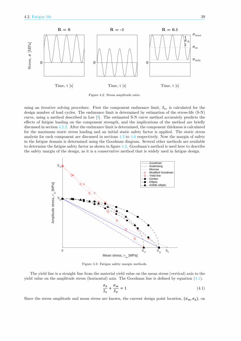
4.2. Fatigue life 39
0
Time, t [s]
Stre
ss,𝜎
[MPa
]R = 0
0
Time, t [s]
R = -1
0
𝜎m
𝜎min
𝜎max
𝜎A↑↓
Time, t [s]
R = 0.1
Figure 4.2: Stress amplitude ratio.
using an iterative solving procedure. First the component endurance limit, 𝑆 , is calculated for thedesign number of load cycles. The endurance limit is determined by estimation of the stress-life (S-N)curve, using a method described in Lee [9]. The estimated S-N curve method accurately predicts theeffects of fatigue loading on the component strength, and the implications of the method are brieflydiscussed in section 4.2.2. After the endurance limit is determined, the component thickness is calculatedfor the maximum static stress loading and an initial static safety factor is applied. The static stressanalysis for each component are discussed in sections 4.3 to 4.6 respectively. Now the margin of safetyin the fatigue domain is determined using the Goodman diagram. Several other methods are availableto determine the fatigue safety factor as shown in figure 4.3. Goodman’s method is used here to describethe safety margin of the design, as it is a conservative method that is widely used in fatigue design.
0 SY
SU
Sf
Mean stress, σm
[MPa]
Se
SY
Am
plitu
de s
tres
s, σ
A [M
Pa]
GoodmanSoderbergMorrowModified GoodmanYield lineGerberEllipticASME-elliptic
Figure 4.3: Fatigue safety margin methods.
The yield line is a straight line from the material yield value on the mean stress (vertical) axis to theyield value on the amplitude stress (horizontal) axis. The Goodman line is defined by equation (4.1).
𝜎𝑆 + 𝜎𝑆 = 1 (4.1)
Since the stress amplitude and mean stress are known, the current design point location, (𝜎 , 𝜎 ), on

40 4. Structural analysis & Weight
the figure is also known. The fatigue loading safety margin is then determined by equation (4.2).
𝑆𝐹 = 𝐿 + 𝐿𝐿 (4.2)
Where 𝐿 is the distance from the origin to the current design point, and 𝐿 is the shortest distancefrom the design point to Goodman line. In a similar fashion the safety factor of the yield line isdetermined. The desired value is then compared to the current smallest safety factor, and a new guessfor the static safety factor is made. This iterative procedure is used for the fatigue design of all partsexcept for disk fatigue life prediction. The disk life is approximated using a different method, which isfurther explained in section 4.4.
4.2.2. Estimated stress-lifeStress-life curves describe the decrease in component failure strength as a result of the number of loadcycles applied on the component. Based on extensive destructive load cycle testing, S-N curves aredeveloped. However, there are many factors that have effect on the failure strength of a component,and a different stress-life cycle should be determined for each case. Since testing is an expensive andtime-consuming process, methods have been developed to estimate the S-N curves. A quick method ofestimating the stress-life curve of a component based on the material ultimate strength is presented byLee [9].
A typical stress-life (S-N) curve of an arbitrary steel component is shown in figure 4.4. It can beseen that the fatigue life of a component is dependent on several factors, such as the material used, theloading conditions, geometry, surface finishing. The method uses correction factors to compensate forthese effects.
mirror-polished, notch free
Life, N, cycles (log)
Str
ess a
mplitu
de, S
a (lo
g)
CL Load
103
CD Size
CS Surface
Sbe
S1000
Se
CR Reliability
106
slope factor k
Haibach, slope factor 2k-1
Miner, slope factor k
Figure 4.4: Modified S-N curves for steel component. Source: [9]
In the method, the baseline fatigue strength at 10 cycles, 𝑆 , is determined based on the ultimatetensile strength and depending on material type and type of loading. The loading type itself is also ofgreat influence on the shape of the S-N curve, the effect of which is captured in the loading correctionfactor, 𝐶 . Table 4.2 gives an overview of the the baseline fatigue strength and loading factor, based onthe material and loading conditions, while the reliability correction factor is presented in table 4.3.
Due to the random nature of the fatigue life of components, non-destructive testing data usually arescattered. A reliability correction factor, 𝐶 , is introduced to incorporate this statistical effect of thedistributed results on the S-N curve. Table 4.4 shows the suggested values of the correction factor fordifferent reliability levels.
From figure 4.4 it can be seen that after a certain number of cycles, the fatigue properties do notdecrease anymore. This is called the fatigue limit, and the uncorrected baseline of the fatigue limit isdetermined by the bending fatigue limit as shown in table 4.4.

4.2. Fatigue life 41
Table 4.2: Baseline fatigue strength, , andloading factor, , based on the material and loading
conditions.
Loading MaterialBending All . ⋅ .Axial All . ⋅ .Axial+Bending All . ⋅ .Torsion Steel . ⋅ .Torsion Nonferrous . ⋅ .Torsion Cast iron . ⋅ .
Table 4.3: Reliability factor,
Reliability. .. .. .. .. .. .. .. .
Table 4.4: Baseline bending fatigue limit, , and cycle limit,
MaterialSteel . ⋅SteelCast iron . ⋅ ⋅Nonferrous . ⋅ ⋅Nonferrous ⋅
The size factor, 𝐶 , is used to correct for different specimen sizes of the component, and is definedby equation (4.3).
𝐶 = 1.0 for 𝑑 < 8mm1.189𝑑 . for 8mm < 𝑑 < 250mm
(4.3)
The last correction factor is the surface finishing factor, 𝐶 . All engine components are assumed to bewell polished and hence the surface finishing correction factor is fixed at 𝐶 = 1.0.
Finally, the corrected fatigue limit, 𝑆 , can be estimated by multiplying the baseline bending fatiguelimit with all correction factors, which results in equation (4.4).
𝑆 = 𝑆 𝐶 𝐶 𝐶 𝐶 (4.4)
Now the slope of the line can be determined using the logarithmic difference of the corrected fatiguestrength at 10 cycles, 𝑆 , = 𝑆 𝐶 , and the corrected fatigue limit, 𝑆 , according to equation(4.5).
𝑘 = − log(10 ) − log(𝑁 )log(𝑆 ) − log(𝑆 ) (4.5)
The stress at any point on this line is then determined by equation (4.6).
𝑁 = 𝑁 (𝑆𝑆 ) (4.6)
The estimated stress-life method has been compared to actual S-N curve data for Ti-6Al-4V at a cyclicstress ratio of 𝑅 = 0. The resulting estimated S-N curve is shown in figure 4.5.
The data has been fitted based on a simplified version of the random fatigue limit (RFL) model, asproposed by Pascual and Meeker [92]. The RFL model describes the fatigue limit of each individualspecimen, and maximum likelihood methods are used to estimate the parameters of the S-N as describedby equation (4.7).
ln𝑁 = 𝛽 + 𝛽 ln(𝜎 − 𝛾) + 𝜀 (4.7)
where 𝛽 and 𝛽 are fatigue curve coefficients, 𝛾 the fatigue limit of the specimen and 𝜀 the error term.The simplified model used for fitting uses another logarithmic which resulted in better data fitting, andis described by equation (4.8).
ln(𝑁 − 𝜀) = 𝛽 (ln(𝜎) − 𝛾) (4.8)
As can be seen in the figure, the estimated S-N curve is well in agreement with the actual testdata. The standard deviation of fitted curve of the test data has been used to calculate the actual

42 4. Structural analysis & Weight
10 10 10 10 10 1010
10 .
10 .
10 .
10 .
10
Number of cycles, N [-]
Stre
ssam
plitu
de,𝜎
A[M
Pa]
FittedDataReliabilityReliability + correctionEstimatedEstimated + correction
Figure 4.5: S-N data curve fitting vs. fatigue life estimation
reliability factor. Comparing the actual reliability to the estimated correction factor values also showsgood agreement, and the same holds for application of the correction factors.
For the design case of the different engine components, the number of design life cycles should bedetermined. Since turbofan engines are typically designed for over 20 years of operation, the number ofdesign load cycles extends beyond the low-cycle fatigue (LCF) limit into the high-cycle fatigue (HCF)range. According to Tong [11], a typical range for commercial production engines is between 15000–20000 flight cycles. The upper limit of this range is taken as the design conditions for all components.Table 4.5 shows an overview of the fatigue input conditions of each component.
Table 4.5: Component materials and fatigue design input parameters.
Stage Component Material Loading type Life cyclesFan Blades Ti-6Al-4V Axial 200,000
Disks Ti-17 – 200,000Pressure casing Al-6061 Axial+Bending 200,000Blade containment casing Kevlar Impact –
LPC Blades Ti-6Al-4V Axial 200,000Disks Ti-17 – 200,000Pressure casing Ti-6Al-4V Axial+Bending 200,000
Misc Nose Al-6061 – –Shaft Ti-17 Torsion 200,000
4.3. BladesAccording to Armand [93] the blade volume can be approximated by taking the height of the blade, ℎ ,multiplied by the squared value of the blade chord length, 𝑐 , and applying a volumetric correctionfactor, 𝑉𝐹, leads to equation (4.9).
𝑉 = ℎ ⋅ 𝑐 ⋅ 𝑉 (4.9)
The volumetric correction factors are defined by Onat & Klees [49] as fixed values for different type ofcompressor stages. The correction factors are defined as:
𝑉 = 0.024 for fan blades0.047 for LPC blades0.163 for HPC blades
The resulting blade mass includes the root section of the blade. However, more accurate results for bladeweight estimation might be obtained by calculating the airfoil and blade root weight separately. In this
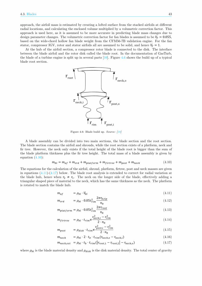
4.3. Blades 43
approach, the airfoil mass is estimated by creating a lofted surface from the stacked airfoils at differentradial locations, and calculating the enclosed volume multiplied by a volumetric correction factor. Thisapproach is used here, as it is assumed to be more accurate in predicting blade mass changes due todesign parameter changes. The volumetric correction factor for fan blades is assumed to be 𝑉 = 0.055,based on the wide-chord hollow fan blade weight from the CFM56-7B validation engine. For the fanstator, compressor IGV, rotor and stator airfoils all are assumed to be solid, and hence 𝑉 = 1.
At the hub of the airfoil section, a compressor rotor blade is connected to the disk. The interfacebetween the blade airfoil and the rotor disk called the blade root. In the documentation of GasTurb,the blade of a turbine engine is split up in several parts [10]. Figure 4.6 shows the build up of a typicalblade root section.
rpost,o
rrim
rpost,i
rneck,i
rneck,o
rroot
Figure 4.6: Blade build up. Source: [10]
A blade assembly can be divided into two main sections, the blade section and the root section.The blade section contains the airfoil and shrouds, while the root section exists of a platform, neck andfir tree. However, the neck only exists if the total height of the blade root is bigger than the sum ofthe blade platform thickness plus the fir tree height. The total mass of a blade assembly is given byequation (4.10):
𝑚 = 𝑚 +𝑚 +𝑚 +𝑚 +𝑚 +𝑚 (4.10)
The equations for the calculation of the airfoil, shroud, platform, firtree, post and neck masses are givenin equations (4.11)-(4.17) below. The blade root analysis is extended to correct for radial variation atthe blade hub, hence when 𝑟 ≠ 𝑟 . The neck on the longer side of the blade, effectively adding atriangular shaped piece of material to the neck, which has the same thickness as the neck. The platformis rotated to match the blade hub.
𝑚 = 𝜌 ⋅ 𝑉 (4.11)
𝑚 = 𝜌 ⋅ 0.05𝑡2𝜋𝑟 ,𝑛 (4.12)
𝑚 = 𝜌 ⋅ 0.05𝑡 2𝜋𝑟𝑛 (4.13)
𝑚 = 𝜌 ⋅ 𝑡 𝜋𝑟 , − 𝑟
2 ⋅ 𝑛 (4.14)
𝑚 = 𝜌 ⋅ 𝑡 𝜋𝑟 , − 𝑟2 ⋅ 𝑛 (4.15)
𝑚 = 𝜌 ⋅ 2 ⋅ 𝑡 ⋅ 𝑡 (𝑟 , − 𝑟 , ) (4.16)𝑚 , = 𝜌 ⋅ 𝑡 ⋅ 𝑡 (|𝑟 , − 𝑟 , | − 𝑟 , ) (4.17)
where 𝜌 is the blade material density and 𝜌 is the disk material density. The total center of gravity

44 4. Structural analysis & Weight
of the blade is then given by equation (4.18).
𝑟 , =∑𝑚 𝑟 ,𝑚 (4.18)
4.4. DisksThe stress analysis of a rotating disk is described in many literature, and is usually solved consideringinfinitesimal ring-shaped disk part of constant thickness, as indicated in figure 4.7.
Figure 4.7: Rotating disk stress analysis. Source: [11]
Boorsma [19] presents three methods to solve the disk stress calculations in his work. One methodfrom Mattingly [31], which allows for hyperbolic disk design at constant stress levels throughout thedisk, secondly a finite difference method by Tong et al. [11], and finally a low fidelity method to optimizethe disk shape, which is also used in T-AXI Disk [94, 95]. A fourth method for disk stress calculationshas been added to this literature study. It is a calculation method presented in the work from Lolis[45], which mainly follows the method provided by a textbook from Potter [96].
In Boorsma’s work it is concluded that the method used in T-AXI Disk will be best suitedfor preliminary disk stress calculations. This conclusion remains unchanged as the iterative solvingstructure for each element provided in Lolis’ method, will result in slower calculations compared to thematrix calculations from the T-AXI Disk method. The governing equations for the disk stress analysisas described by Gutzwiller and used in T-AXI Disk, are shown below. [95]
Using a simple force equilibrium of the element indicated in figure 4.7, it is shown that the tangentialand radial forces are given by equations (4.19) and (4.20).
∑𝐹 = 0 (4.19)
∑𝐹 = 𝜎 ⋅ 𝑟 ⋅ 𝑑𝜃 + 𝜎 ⋅ 𝑑𝑟 ⋅ 𝑑𝜃 − (𝜎 + 𝑑𝜎𝑑𝑟 ⋅ 𝑑𝑟) ⋅ (𝑟 + 𝑑𝑟) ⋅ 𝑑𝜃 − 𝜌 ⋅ Ω ⋅ 𝑟 ⋅ 𝑑𝑟 ⋅ 𝑑𝜃 = 0 (4.20)
After some algebraic manipulation, equation (4.20) can be rewritten in the form of equation (4.21).
0 = 𝑑𝑑𝑟(𝑡𝑟 ⋅ 𝜎 ) − 𝑡 ⋅ 𝜎 + 𝑡𝜌Ω 𝑟 (4.21)
4.4. Disks 45
The formula for the hoop stress, 𝜎 , and radial stress, 𝜎 , are given in by equations (4.22) and (4.23)respectively.
𝜎 = 𝐴𝑑𝑢𝑑𝑟 + 𝐵𝑢𝑟 − 𝐴𝛼 𝑇 − 𝐵𝛼 𝑇 (4.22)
𝜎 = 𝐵𝑑𝑢𝑑𝑟 + 𝐷𝑢𝑟 − 𝐵𝛼 𝑇 − 𝐷𝛼 𝑇 (4.23)
The boundary conditions at the bore and at the rim of the disk are given by equations (4.24) and (4.25).
𝜎 = 𝐴𝑑𝑢𝑑𝑟 + 𝐵𝑢𝑟 − 𝐴𝛼 𝑇 − 𝐵𝛼 𝑇 = −
𝑛 𝑚 𝑟 ,2𝜋𝑟𝑡 Ω (4.24)
𝜎 = 𝐴𝑑𝑢𝑑𝑟 + 𝐵𝑢𝑟 − 𝐴𝛼 𝑇 − 𝐵𝛼 𝑇 =
𝑛 𝑚 𝑟 ,2𝜋𝑟𝑡 Ω (4.25)
Where 𝑟 , is given by equation (4.18), and constants 𝐴, 𝐵 and 𝐷 in the above equations are all functionsof material properties such as material strength, 𝐸, and Poisson’s ratio, 𝜈, and their respective relationsare shown in equations (4.4) – (4.4). Further details about the calculation process can be found in [94].
𝐴 = 𝐶 𝐶 − 𝐶𝐶 (4.26)
𝐵 = 𝐶 𝐶 − 𝐶 𝐶𝐶 (4.27)
𝐷 = 𝐶 𝐶 − 𝐶𝐶 (4.28)
𝐶 = 𝐶 = 𝐸 (𝐸 − 𝐸 𝜈 )𝐸 − 2𝐸 𝜈 (4.29)
𝐶 = 𝐸𝐸 − 2𝐸 𝜈 (4.30)
𝐶 = 𝐶 = 𝐸 𝐸 𝜈𝐸 − 2𝐸 𝜈 (4.31)
𝐶 = 𝐸 𝜈𝐸 − 2𝐸 𝜈 (4.32)
The disk design is checked for feasibility based on three parameters. First the burst margin, 𝐵𝑀, iscalculated. According to Tong [11], the average tangential stress, 𝜎 , , should be at least 47% lowerthan ultimate strength of the material at the average disk temperature. The burst margin is calculatedusing equation (4.33).
𝐵𝑀 = (0.47 ⋅ 𝜎𝜎 ,− 1) ⋅ 100 (4.33)
The second design parameter is the design margin, 𝐷𝑀, which compares the maximum allowable VonMises stress, 𝜎 , to the yield stress of the material, 𝜎 . A safety factor on the yield stress may beused, which results in equation (4.34).
𝐷𝑀 = (0.9 ⋅ 𝜎𝜎 − 1) ⋅ 100 (4.34)
The burst speed, 𝐵𝑆, of the disk is the last design parameter. The burst speed parameter takes intoaccount the possible overspeed operation, at which the disk turn at more than the 100% rotationalspeed limit they are designed for. During the design mission, overspeed operations may occur for shortperiods of time, hence it is important to make sure the disk is designed to cope with the excessive stressloads that occur during such operational speeds. According to GasTurb, the disk should be designedfor burst speeds up to 130%. [10]
𝐵𝑆 = 100 ⋅ √𝜎𝜎 ,
(4.35)

46 4. Structural analysis & Weight
To take the effects of material fatigueness caused by cyclic loading of the disk into account, a fatiguelife estimation method by Armand [93] is used. In this method, the equivalent strain range is calculatedusing the maximum-distortion-energy theory, shown in equation (4.36).
Δ𝜀 = √23 √(𝜀 − 𝜀 ) + (𝜀 − 𝜀 ) + (𝜀 − 𝜀 ) (4.36)
The value for the strain range obtained by equation (4.36) is compared to another definition of strainrange, for a specimen loaded in only the axial direction. Equation (4.4) shows the relationship foundby Mendelson & Manson [97] that relates the low-cycle fatigue life and other material properties to thestrain range.
Δ𝜀 = 3.5𝑆𝐸 𝑁. + 𝐷 . 𝑁 . (4.37)
where, 𝑆 is the ultimate tensile strength, 𝐸 the Young’s modulus, and 𝐷 the ductility of the material.Since the temperature in the fan and LPC stage are relatively low, the material ductility is assumed tobe constant. The ductility is a function of the reduction in area at failure, 𝑅𝐴, and is calculated usingequation (4.38).
𝐷 = ln( 11 − 𝑅𝐴) (4.38)
4.5. CasingThe casing of the fan and LPC stages have a great effect on the total engine weight. Therefore, itis important to carefully design such a component, while satisfying the main design requirements.Although the component casing has multiple functionalities in the total engine, the two main designcriteria of the casing are the pressure containment and blade fraction containment. Several designphilosophies exist for fan and compressor casings [45, 47, 98], and in this thesis two design methods areadopted.
In the fan stage two separate casings are designed. A steel casing is used to provide pressurecontainment in the fan stage and bypass duct. Section 4.5.1 further elaborates on the required casingthickness determination for pressure containment. Another, more critical design condition for the fanstage casing is the blade fraction containment. In case of a blade release, the fan casing should be ableto withstand the blade impact. Blade fraction containment is ensured by introducing a kevlar linerinside the steel pressure pressure containment casing. The design methodology of the blade fractioncontainment casing is elaborated upon in section 4.5.2.
The casing in the LPC stages are only designed for pressure containment. However, as mentionedearlier the design point for the LPC casing is taken from the last HPC stage, as the casing is made ofone piece and in practice the casing thickness often does not vary between these two components.
Apart from the static loading conditions, the casing fatigue life is also taken into account. Theoutput of the static design case is used for the fatigue design which has been treated in section 4.2.
4.5.1. Pressure containmentWhen considering a static loads on the component, the casing thickness can directly be determinedfrom Barlow’s equation. Using this method, the casing is modelled as a pressurize pipe, and relates theinternal pressure in the pipe or pressure vessel to the maximum stress level occurring in the material.Equation (4.39) shows the original formulation of Barlow’s equation.
𝑝 =2 ⋅ 𝜎 ⋅ 𝑡𝐷 (4.39)
Where 𝐷 is the casing outer diameter. However, for this design problem it is more convenient to rewritethe equation to solve for the minimum required thickness, given a material under a certain pressure,which leads to equation (4.40).
𝑡 , = 𝑝 ⋅ 𝑟𝜎 − 𝑝 (4.40)
Where 𝑟 is the casing inner radius and 𝑝 the static internal pressure, given by 𝑝 = 𝑝 − 𝑝 .The above described design method results in very thin pressure casing thickness for the fan stage
since the pressure difference between the inner fan casing and the ambient conditions are relatively
4.6. Shaft 47
small. Onat & Klees [49] suggest a method by Stewart [99] which describes the collapsing pressure forthin-walled large diameter tubes. The collapsing pressure is given by equation (4.41).
𝑝 = 6.895 ⋅ 10 (1 − √1 − 1600 𝑡𝐷 ) (4.41)
Where 𝑡 is the the casing thickness, 𝐷 the casing diameter and 𝑝 the collapsing pressure. Althoughthe external pressure will not exceed the fan duct inner pressure, the design condition for collapsingpressure is way more sensitive than the pressure containment design. Assuming a maximum pressuredifference between inner and outer duct of 0.8 at static sea level conditions corresponds to a minimumcasing thickness of 3.0𝑚𝑚, which is used as a fixed minimum thickness in the design routine.
4.5.2. Blade containmentThe blade containment casing is by far the most critical design condition for the fan stage. Since thepressure in the fan is relatively low, the minimum thickness requirements for the fan casing are low aswell. The requirement for fan blade containment however is quite demanding, as the casing should bedesigned to withstand a full fan blade release at overspeed conditions.
Full scale analysis of blade impact and casing deformation extends beyond the scope of this thesis.For the conceptual design of the fan casing, a simple estimation method presented by Lolis [45] is used.First the fan blade kinetic energy at release is determined. Other methods sometimes include an extraterm for the rotational kinetic energy. [100] The total kinetic energy is then given by equation (4.42)
𝐸 , = 12𝑚 𝑉 + 12𝐼 𝜔 (4.42)
where 𝑚 is the blade mass, 𝑉 the blade impact velocity, 𝐼 the blade mass moment of inertia and𝜔 the blade rotational velocity. For design using an energy balance, the kinetic energy of the bladeshould be balanced by the strain energy of the plastic deformed casing material. However, the methodused here takes a more simple approach. The blade internal rotation is assumed zero, and hence therotational kinetic energy is zero. The minimum required casing thickness is then defined by equation(4.43).
𝑡 , = 0.4𝐸 , 𝐸𝜎 ℎ 𝑐 (4.43)
4.6. ShaftThe low pressure shaft drives both the fan and compressor stages. The spool geometry is optimizedfor minimum weight. However, there are some constraints to the LP spool diameter. A larger outerdiameter might be advantageous for the component torsional strength, the diameter should remainsmall enough as the HP spool is enclosing the LP spool.
The load on the LP spool is calculated based on the total compressor and fan specific work, .Equation (4.44) shows the relationship between the shaft stress as a result of the torsional loading,given an inner and outer diameter[47].
𝜎 = 16𝐷 𝜔𝜋(𝐷 − 𝐷 ) (4.44)
After the static design of the shaft is determined, the fatigue life is estimated using the method describedin section 4.2. The optimum diameter and thickness of the shaft for minimum weight design are foundusing a simple optimization routine.
4.7. Spinner coneThe spinner cone is a hollow cone structure in front of the fan stage, which consists of a front and arear cone part. The spinner front cone is usually designed to minimize the ice build-up and should beable to withstand bird-strike. The spinner rear cone is designed to smoothen the airflow at the faninlet, usually resulting in a spline surface interface between the spinner front cone and the fan blade

48 4. Structural analysis & Weight
platform. A simplified approach is used here, assuming a linear connection between the spinner frontcone and fan blade platform, effectively extending the blade platform. The thickness of the nose cone isassumed to be fixed at 5𝑚𝑚, as suggested by Lolis [45]. This value is well in accordance with the 4.9𝑚𝑚spinner front cone thickness measured on the CFM56-7 validation engine. The spinner front cone ismade of black sulfuric anodized aluminium, but for the weight estimation here a standard aluminiumalloy Al-6061 is used.

5Noise Estimation
As shown in figure 2.4, noise propagation from high bypass ratio turbofan engines is dominated by thefan noise. At take-off however, jet stream noise can reach comparable levels to the fan noise. In thisresearch, only the fan noise is considered and the noise propagation is predicted using three differentnoise estimation methods.
The noise prediction software Soprano uses two noise prediction methods developed by NASA: theAircraft Noise Prediction Program (ANOPP) by Heidmann [54] and the improved ANOPP method byKontos [55]. Diéz [5] introduced the use of a third method developed the Engineering Society of DataUnits (ESDU) [101], and did a comparison with the three noise estimation techniques. Diéz concludedthat there no large differences between the noise estimation methods were appreciated. The methodsare well documented by Diéz [5], and hence his approach is adopted here to predict the noise outputfrom the fan stage.
Another feature of the noise prediction tool is the fly-over simulation. The noise spectrum of theengine on itself is not a good indicator of the engine performance in terms of noise, as the perceivednoise levels on the ground differ from the measurements directly at the source. For this reason, mainnoise descriptors are used to characterize the noise generated by the engine during a fly-over, whichwill be simulated using the noise spectrum output from the prediction methods. The determination ofnoise descriptors is further elaborated upon in section 5.6. The take-off and fly-over procedure is thendescribed by section 5.5.
5.1. Noise prediction methodsThree empirical methods to estimate the noise propagation from the fan stage are considered here.Section 5.2 will elaborate on the ANOPP method by Heidmann. The other two considered methodsoriginated from the original ANOPP method. Since the basic concepts of the empirical methods aretherefore very much alike, only the differences between the methods will be explained for the other twomethods in section 5.3 and 5.4 for the improved ANOPP method and ESDU method respectively.
5.2. Heidmann’s methodThe ANOPP method was originally presented by Heidmann in 1975 [54]. The method is used tocompute the one-third octave band spectral intensities of the free field noise pattern. The intensitiesvary as a function of the polar angle about the fan or compressor axis, are assumed to be symmetricabout this axis, and are given as the sound pressure levels (SPL) at a 1𝑚 radius.
The predicted free-field radiation can be divided into the following noise components:
1. Inlet duct noise
(a) Broadband noise(b) Discrete-tone noise(c) Combination-tone noise
2. Discharge duct noise
49

50 5. Noise Estimation
(a) Broadband noise(b) Discrete-tone noise
Heidmann [102] tested full-scale fans at NASA Lewis Center to find parameters that correlate tothe noise output of the fan. In the study, the fan is assumed to be a noise generator in which inputmechanical power is converted to output sound power. Heidmann concluded that the sound poweroutput is strongly related to the specific work performed during the compression process. Since thespecific work and mechanical power are proportional to the total temperature rise in the stage Δ𝑇 andthe mass flow rate a general form of the normalized sound pressure level 𝑆𝑃𝐿 can be expressed interms of equation (5.1).
𝑆𝑃𝐿(𝑓, 𝜃) = 20 log(Δ𝑇Δ𝑇 ) + 10 log( ) + 𝑓(design detail) (5.1)
in which Δ𝑇 and are reference values which are fixed at Δ𝑇 = 0.555𝐾 and = 0.453𝑘𝑔/𝑠respectively. The frequency spectral function 𝑓(design detail) depends on three main noise contributorsas explained earlier. The contributions of broadband noise, discrete tone noise and combination tonenoise are explained in sections 5.2.1, 5.2.2 and 5.2.3 respectively. A full detailed description of theANOPP method can be found in Heidmann [54].
5.2.1. Broadband noiseThe broadband noise is calculated by predicting the average behaviour of the one-third octave broadbandnoise
𝑆𝑃𝐿(𝑓, 𝜃) = 20 log(Δ𝑇Δ𝑇 ) + 10 log( ) + 𝐹 (𝑀 ,𝑀 , ) (5.2)
+ 𝐹 (𝑅𝑆𝑆) + 𝐹 (𝜃) + 𝐹 (𝑓, 𝑓 ) (5.3)
where 𝐹 is a discrete function based on the operating and design relative tip Mach number, 𝐹 adirectivity correction function for the broadband noise, and 𝐹 a correction function for the rotor-statorspacing parameter, 𝑅𝑆𝑆. The rotor-stator spacing parameter 𝐹 is determined by equation (5.4) or (5.5),depending on the inlet distortion conditions.
𝐿 = 𝐶 log(𝑅𝑆𝑆300 ) without inlet flow distortions (5.4)
𝐿 = 𝐶 log( ) for 𝑅𝑆𝑆 ≤ 100𝐶 log( ) for 𝑅𝑆𝑆 > 100 with inlet flow distortions (5.5)
where the relative rotor-to-stator spacing 𝑅𝑆𝑆 is expressed in percentage of the tip rotor chord, and𝐶 = −5 for broadband noise.
Finally, 𝐹 is determined using equation (5.6) and represents the broadband noise spectrum shape.
𝐹 (𝑓, 𝑓 ) = 10 log [𝑒 . (ln( . )
ln𝜎 ) ] (5.6)
Here 𝜎 is the geometric mean deviation which is equal to 2.2, and 𝑓 is the blade passage frequency,which is a function of the rotational speed, 𝑁, and the number of rotor blades, 𝐵. The definition of theblade passage frequency is given in equation (5.7)
𝑓 = 𝑁60𝐵 (5.7)
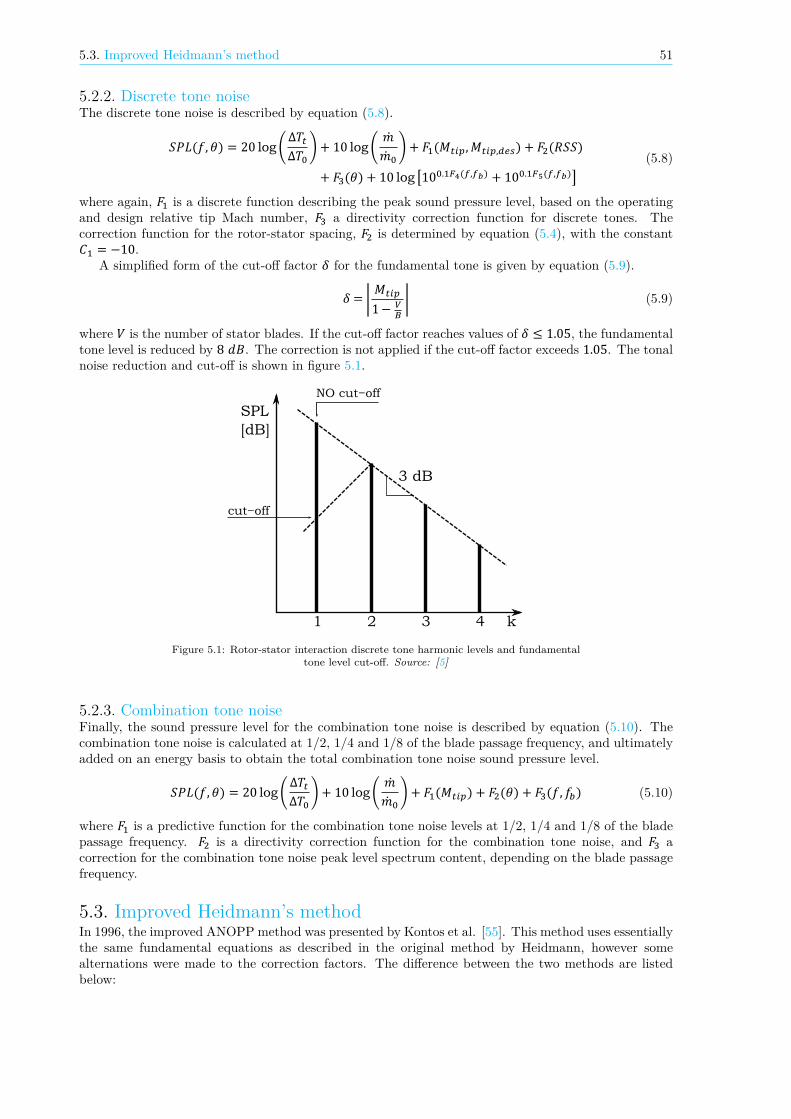
5.3. Improved Heidmann’s method 51
5.2.2. Discrete tone noiseThe discrete tone noise is described by equation (5.8).
𝑆𝑃𝐿(𝑓, 𝜃) = 20 log(Δ𝑇Δ𝑇 ) + 10 log( ) + 𝐹 (𝑀 ,𝑀 , ) + 𝐹 (𝑅𝑆𝑆)
+ 𝐹 (𝜃) + 10 log [10 . ( , ) + 10 . ( , )](5.8)
where again, 𝐹 is a discrete function describing the peak sound pressure level, based on the operatingand design relative tip Mach number, 𝐹 a directivity correction function for discrete tones. Thecorrection function for the rotor-stator spacing, 𝐹 is determined by equation (5.4), with the constant𝐶 = −10.
A simplified form of the cut-off factor 𝛿 for the fundamental tone is given by equation (5.9).
𝛿 = | 𝑀1− | (5.9)
where 𝑉 is the number of stator blades. If the cut-off factor reaches values of 𝛿 ≤ 1.05, the fundamentaltone level is reduced by 8 𝑑𝐵. The correction is not applied if the cut-off factor exceeds 1.05. The tonalnoise reduction and cut-off is shown in figure 5.1.
SPL
[dB]
3 dB
NO cut−off
cut−off
1 2 3 4 k
Figure 5.1: Rotor-stator interaction discrete tone harmonic levels and fundamentaltone level cut-off. Source: [5]
5.2.3. Combination tone noiseFinally, the sound pressure level for the combination tone noise is described by equation (5.10). Thecombination tone noise is calculated at 1/2, 1/4 and 1/8 of the blade passage frequency, and ultimatelyadded on an energy basis to obtain the total combination tone noise sound pressure level.
𝑆𝑃𝐿(𝑓, 𝜃) = 20 log(Δ𝑇Δ𝑇 ) + 10 log( ) + 𝐹 (𝑀 ) + 𝐹 (𝜃) + 𝐹 (𝑓, 𝑓 ) (5.10)
where 𝐹 is a predictive function for the combination tone noise levels at 1/2, 1/4 and 1/8 of the bladepassage frequency. 𝐹 is a directivity correction function for the combination tone noise, and 𝐹 acorrection for the combination tone noise peak level spectrum content, depending on the blade passagefrequency.
5.3. Improved Heidmann’s methodIn 1996, the improved ANOPP method was presented by Kontos et al. [55]. This method uses essentiallythe same fundamental equations as described in the original method by Heidmann, however somealternations were made to the correction factors. The difference between the two methods are listedbelow:

52 5. Noise Estimation
1. For the broadband noise propagating from the inlet (1a), the correcting function 𝐹 is modifiedand the term 𝐹 is eliminated.
2. For the broadband noise radiation from the discharge duct (2a), the correcting factor 𝐹 is modified.3. For the discrete tone noise radiation (1b & 2b), the tonal reduction quantity is modified. Instead of
a 3 dB reduction, the improved ANOPP method suggests a reduction of 6 dB or 9 dB, dependingon the tip Mach number.
4. For the discrete tone noise propagating from the inlet (1b), the term 𝐹 is eliminated.5. For the discrete tone noise radiation (1b & 2b), a further reduction of the blade pass frequency
(BPF) tone and its second harmonic is proposed. The new reductions are dependent on the polarangle, and have to be interpolated from a table presented in the paper.
6. For the combination-tone noise (1c), the normalized combination tone noise levels, 𝐹 , are revised.
5.4. ESDU methodThe ESDU method [101] is presented by the Engineering Sciences Data Unit (ESDU) in 1998, and isalso based on the Heidmann’s method. Therefore only the differences between the ANOPP and thismethod are mentioned here:
1. For the broadband noise propagating from the discharge duct (2a), a new directivity pattern isapplied.
2. For the broadband noise radiation (1a & 2a), the spectrum content function, 𝐹 , is modified3. For the discrete-tone noise radiation (1b & 2b), the directivity function is modified. For the
superior harmonics, the tonal noise reduction is also changed.4. For the combination-tone noise (1c), the normalized combination tone noise levels, 𝐹 , are revised.
5.5. Take-off simulationA simulation of a take-off procedure will be used to determine the noise performance of the enginefan stage as measured by an observer on the ground. The simulation is set-up is according to theInternational Civil Aviation Orginazation (ICAO) regulations. Lateral and fly-over noise measurementsare mandatory for the certification procedure described in ICAO regulations (Annex 16 to ChicagoConvention, Volume I, chapter 3). Figure 5.2 and 5.3 show the take-off procedure flightpath with thelocation of the observer and important ground speeds and flight angles indicated.
For the take-off simulation a Boeing 767-300ER aircraft is used as the reference aircraft, equippedwith two CF6-80C2/B6F engines [103]. All relevant input used for the determination of the take-offprocedure flightpath is mentioned in table 5.1.
Table 5.1: Take-off simulation input parameters.
Property Symbol Value UnitsRotation speed 𝑉 82.24 𝑚/𝑠Lift-off speed 𝑉 84.81 𝑚/𝑠Climb speed 𝑉 92.52 𝑚/𝑠Lift-off angle 𝛾 8 𝑑𝑒𝑔Climb-out angle 𝛾 14 𝑑𝑒𝑔Longitudinal distance 𝐿 6500 𝑚Lateral distance 𝐿 450 𝑚Maximum take-off mass 𝑀𝑇𝑂𝑀 186880 𝑘𝑔Maximum take-off thrust 𝐹 269657 𝑁
From the flight path the distance and angle as measured from the indicated observer points canbe calculated, from which the variation of the distance and angle over simulation time can be found.Figures 5.4 and 5.5 show the distance and angle history respectively.

5.6. Noise descriptors 53
Pre−rotation Rotation Lift−offClimb
8º
14 º
Receiver
6500 m
V = 0 V = VR
V = V2
V = VC
Figure 5.2: Take-off procedure. Source: [5]
Maximum PNL
450 m
Lateral Noise
Figure 5.3: Lateral noise measurement location. Source: [5]
0 50 100 150
2,000
4,000
6,000
8,000
Time [s]
Dist
ance
[m]
Fly-overLateral
Figure 5.4: Distance history for 767-300ER take-offprocedure.
0 50 100 1500
50
100
150
Time [s]
Ang
le[d
eg]
Fly-overLateral
Figure 5.5: Angle history for 767-300ER take-off pro-cedure.
5.6. Noise descriptorsNoise descriptors are used to give a better understanding of how a noisy event is perceived by humanson the ground. The ICAO has defined several noise descriptors for certification purposes. This sectionwill elaborate on the calculation process of the noise descriptors.
The equivalent perceived noise level (EPNL) is the most important noise performance indicator,which is a modification to the perceived noise level (PNL) and takes the noise level as perceived by ahuman observer as well as the duration of the noisy event into account. To calculate the EPNL, thesound pressure level from the simulation should first be corrected for the Doppler shift, which is inducedby the moving noise source. The frequency shift as a result of a moving noise source perceived by a

54 5. Noise Estimation
static observer is given in equation (5.11).
𝑓 = 𝑓1 −𝑀 cos𝜃 (5.11)
where 𝑓 is the frequency perceived by the observer, 𝑓 the noise emission frequency, 𝑀 the flight Machnumber and 𝜃 the emission angle. The Doppler effect shifts the central frequency of each one-third-octave bands, and thus the SPL of the bands are affected. The corrected SPL is calculated usingequation (5.12).
𝑆𝑃𝐿 , = 𝑆𝑃𝐿 , (1 − 𝑆𝐵𝑊 ) + 𝑆𝑃𝐿 ± 𝑆 ± (5.12)
where 𝑆 is the shift in central frequency and 𝐵𝑊 is the bandwidth of the 𝑖-th band.The EPNL is calculated using equation (5.13).
𝐸𝑃𝑁𝐿 = 10 log( Δ𝑡𝑇 ∑ 10 ) (5.13)
where Δ𝑡 is the time step, 𝑇 a time-constant, and TPNL the tone corrected perceived noise level. Thevalues 𝑡 and 𝑡 describe the beginning and end times in which the TPNL lies within 10 𝑑𝐵 of the peakvalue. The tone corrected perceived noise level is given by equation (5.14).
𝑇𝑃𝑁𝐿 = 𝑃𝑁𝐿 + 𝐶 (5.14)
where 𝐶 is the tone correction to the SPL spectrum. The perceived noise level (PNL) is determinedfrom equation (5.15).
𝑃𝑁𝐿 = 40 + 10log2 log𝑁 (5.15)
where N is the overall Noy value. The Noy value in its term is determined using equations (5.16).
𝑁 = 𝑛 + 0.15 [(∑ 𝑛 ) − 𝑛 ] (5.16)
where 𝑁 is the total perceived noisiness, 𝑛 is the perceived noisiness of the 𝑖-th band, and 𝑛 is themaximum perceived noisiness of the 24 considered bands. 𝑛 may be determined by converting tablesfor the earlier described Doppler corrected SPL [104].

6Module validation
The validation of the three design modules is treated separately in the next sections. First the aero-dynamic performance module is validated in section 6.1 using engine test run data from a CFM56-7Bengine. Then the structural analysis and weight estimation module are validated using the same enginein section 6.2. Finally, the noise prediction module is validated in section 6.3 using fan noise data of aCF6-80C2 engine. After the modules have been validated, the effects of increasing tip diameter, varyingspool speed and bypass ratio effects are tested using the design and sizing tool in chapter 7.
6.1. Aerodynamic moduleThe aerodynamic module uses an iterative solving procedure for the fan design. A one-dimensionalflow analysis is carried out at multiple radial sections, and using empirical loss models the pressureloss at each blade-element is calculated. A vortex design method is applied to distribute the spanwiseloading of the fan blade, and radial- and mass flow equilibrium checks ensure the design converges to afeasible solution. The fan design optimization process then maximizes the fan rotor efficiency for a givendesign fan pressure ratio. A redesign of the CFM56-7B fan stage at take-off conditions is consideredhere, and compared to the actual fan design. However, the input design fan pressure ratio has to belimited to 𝐹𝑃𝑅 = 1.35, since higher values for the fan pressure ratio result in infeasible design solutions.Compared to the actual fan pressure ratio of approximately 𝐹𝑃𝑅 = 1.6, this is quite low. The reason forthe limited capabilities of the design code are the constraint acting on the positive camber angle (𝜃 ≥ 0)and the DeHaller design limit (𝐷𝐻 ≥ 0.72). The camber angle constraint is applied for obvious reasons,as the iterative solving process for the blade angles and the loss models do not account for infeasibleconditions. As discussed in section 3.2, the DeHaller number is a non-dimensional design parameterwhich limits the diffusion in a compressor stage to prevent excessive losses. These constraints limit thedesign space of the fan blade optimization process, and a maximum fan pressure ratio of 𝐹𝑃𝑅 = 1.35could be achieved. The aerdodynamic performance of an optimized CFM56-7B turbofan engine fanrotor blade is shown in figure 6.1.
The spanwise distribution of the adiabatic rotor efficiency is shown in figure 6.1c. Due to theincreasing relative velocity with radial location, the temperature difference over the rotor stage increases,boosting the fan efficiency. However, near the rotor tip the efficiencies suddenly decrease as a result ofa steep increase of the loss parameters. The correlations of the shock and profile loss parameters areshown in figures A.1 and A.2 of appendix A respectively.
A relative high adiabatic efficiency is achieved over the rotor blade. However, it should be notedthat these are the results for the rotor alone. The fan stator in the bypass duct and IGV at the LPCinlet decrease the efficiency as the total temperature remains constant, while pressure losses do occurover the static blade rows.
Figure 6.1d shows the DeHaller number and the axial velocity ratio distribution over the blade span.The DeHaller number is pushed towards its lower limit near the blade hub, while at the blade tip thepositive camber angle constraint is limiting the design.
Figure 6.2 shows the optimized fan rotor blade shape. At three indicated radial locations, cross-sectional cuts along the streamline of the blade are made to show the local blade airfoil shape. Low
55

56 6. Module validation
1.26 1.28 1.3 1.32 1.34 1.36 1.38 1.40
0.2
0.4
0.6
0.8
1
Span
wise
loca
tion,
r rel
[-]
CoreBypassCore avg.Bypass avg.Rotor avg.
(a) Pressure ratio, [-]
1.075 1.08 1.085 1.09 1.095 1.1 1.1050
0.2
0.4
0.6
0.8
1
Span
wise
loca
tion,
r rel
[-]
CoreBypassCore avg.Bypass avg.Rotor avg.
(b) Temperature ratio, [-]
0.925 0.93 0.935 0.94 0.945 0.95 0.9550
0.2
0.4
0.6
0.8
1
Span
wise
loca
tion,
r rel
[-]
CoreBypassCore avg.Bypass avg.Rotor avg.
(c) Adiabatic efficiency, [-]
0.7 0.75 0.8 0.85 0.90
0.2
0.4
0.6
0.8
1
Span
wise
loca
tion,
r rel
[-]
Axial velocity ratio, 𝜇DeHaller number, DH
(d) Velocity ratios [-]
0.2 0.4 0.6 0.8 10
0.2
0.4
0.6
0.8
1
Span
wise
loca
tion,
r rel
[-]
Loading coefficient, 𝜓Flow coefficient, 𝜙Degree of reaction, Λ
(e) Non-dimensional performance parameters [-]
0 0.5 1 1.5 2 2.5 30
0.2
0.4
0.6
0.8
1
Span
wise
loca
tion,
r rel
[-]
Incidence angle, 𝜄Deviation angle, 𝛿
(f) Incidence and deviation angles [deg]
0 10 20 30 40 50 60 700
0.2
0.4
0.6
0.8
1
Span
wise
loca
tion,
r rel
[-]
Metal angle (LE), 𝜅1Metal angle (TE), 𝜅2Stagger angle, 𝛾Camber angle, 𝜃
(g) Blade metal angles [deg]
−10 −5 0 5 10 15 20 250
0.2
0.4
0.6
0.8
1
Span
wise
loca
tion,
r rel
[-]
Negative stall limit, 𝛼cPositive stall limit, 𝛼sDesign angle of attack, 𝛼des
(h) Stall angles [deg]
Figure 6.1: Optimized fan results for CFM56-7B engine at take-off design point.
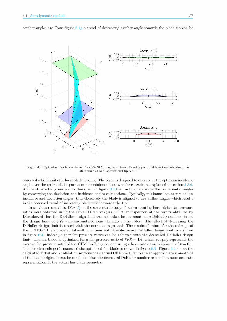
6.1. Aerodynamic module 57
camber angles are From figure 6.1g a trend of decreasing camber angle towards the blade tip can be
Figure 6.2: Optimized fan blade shape of a CFM56-7B engine at take-off design point, with section cuts along thestreamline at hub, splitter and tip radii.
observed which limits the local blade loading. The blade is designed to operate at the optimum incidenceangle over the entire blade span to ensure minimum loss over the cascade, as explained in section 3.3.6.An iterative solving method as described in figure 3.10 is used to determine the blade metal anglesby converging the deviation and incidence angles calculations. Typically, minimum loss occurs at lowincidence and deviation angles, thus effectively the blade is aligned to the airflow angles which resultsin the observed trend of increasing blade twist towards the tip.
In previous research by Díez [5] on the conceptual study of contra-rotating fans, higher fan pressureratios were obtained using the same 1D fan analysis. Further inspection of the results obtained byDíez showed that the DeHaller design limit was not taken into account since DeHaller numbers belowthe design limit of 0.72 were encountered near the hub of the rotor. The effect of decreasing theDeHaller design limit is tested with the current design tool. The results obtained for the redesign ofthe CFM56-7B fan blade at take-off conditions with the decreased DeHaller design limit, are shownin figure 6.3. Indeed, higher fan pressure ratios can be achieved with the decreased DeHaller designlimit. The fan blade is optimized for a fan pressure ratio of 𝐹𝑃𝑅 = 1.6, which roughly represents theaverage fan pressure ratio of the CFM56-7B engine, and using a low vortex swirl exponent of 𝑛 = 0.1.The aerodynamic performance of the optimized fan blade is shown in figure 6.3. Figure 6.4 shows thecalculated airfoil and a validation sections of an actual CFM56-7B fan blade at approximately one-thirdof the blade height. It can be concluded that the decreased DeHaller number results in a more accuraterepresentation of the actual fan blade geometry.

58 6. Module validation
1.4 1.45 1.5 1.55 1.6 1.65 1.70
0.2
0.4
0.6
0.8
1
Span
wise
loca
tion,
r rel
[-]
CoreBypassCore avg.Bypass avg.Rotor avg.
(a) Pressure ratio, [-]
1.12 1.14 1.16 1.180
0.2
0.4
0.6
0.8
1
Span
wise
loca
tion,
r rel
[-]
CoreBypassCore avg.Bypass avg.Rotor avg.
(b) Temperature ratio, [-]
0.8 0.85 0.9 0.95 10
0.2
0.4
0.6
0.8
1
Span
wise
loca
tion,
r rel
[-]
CoreBypassCore avg.Bypass avg.Rotor avg.
(c) Adiabatic efficiency, [-]
0.6 0.65 0.7 0.75 0.8 0.85 0.90
0.2
0.4
0.6
0.8
1
Span
wise
loca
tion,
r rel
[-]
Axial velocity ratio, 𝜇DeHaller number, DH
(d) Velocity ratios [-]
0 0.2 0.4 0.6 0.8 1 1.20
0.2
0.4
0.6
0.8
1
Span
wise
loca
tion,
r rel
[-]
Loading coefficient, 𝜓Flow coefficient, 𝜙Degree of reaction, Λ
(e) Non-dimensional performance parameters [-]
−1 0 1 2 3 4 5 60
0.2
0.4
0.6
0.8
1
Span
wise
loca
tion,
r rel
[-]
Incidence angle, 𝜄Deviation angle, 𝛿
(f) Incidence and deviation angles [deg]
−20 0 20 40 600
0.2
0.4
0.6
0.8
1
Span
wise
loca
tion,
r rel
[-]
Metal angle (LE), 𝜅1Metal angle (TE), 𝜅2Stagger angle, 𝛾Camber angle, 𝜃
(g) Blade metal angles [deg]
−10 0 10 20 30 400
0.2
0.4
0.6
0.8
1
Span
wise
loca
tion,
r rel
[-]
Negative stall limit, 𝛼cPositive stall limit, 𝛼sDesign angle of attack, 𝛼des
(h) Stall angles [deg]
Figure 6.3: Optimized fan results for CFM56-7B engine at take-off design point, with alternative DeHaller design limitof 0.6.

6.1. Aerodynamic module 59
Figure 6.4: Optimized fan blade shape of a CFM56-7B engine at take-off design point, with alternative DeHaller designlimit of . . Section cuts shown along the streamline at hub, splitter, and tip radii, and horizontal projected
section cut at the splitter.
0 0.05 0.1 0.15 0.2-0.1
-0.05
0
x [m]
y[m
]
Section D-D
Optimized, DH≥0.6Optimized, DH≥0.72Validation
Figure 6.5: CFM56-7B fan blade validation section at approximately one-third of blade height.
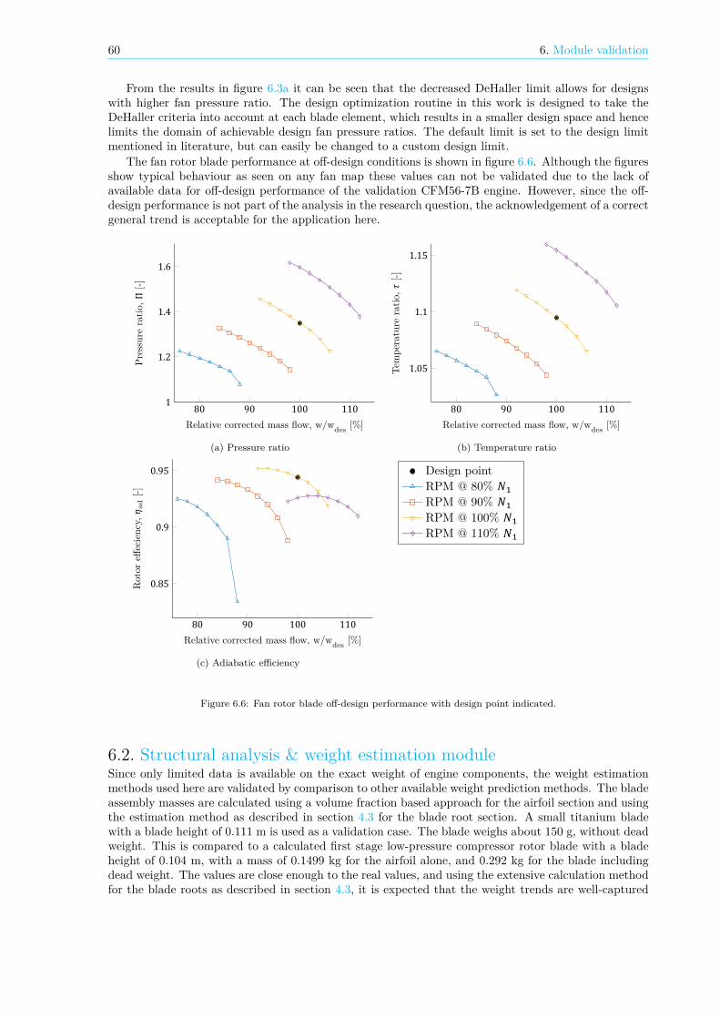
60 6. Module validation
From the results in figure 6.3a it can be seen that the decreased DeHaller limit allows for designswith higher fan pressure ratio. The design optimization routine in this work is designed to take theDeHaller criteria into account at each blade element, which results in a smaller design space and hencelimits the domain of achievable design fan pressure ratios. The default limit is set to the design limitmentioned in literature, but can easily be changed to a custom design limit.
The fan rotor blade performance at off-design conditions is shown in figure 6.6. Although the figuresshow typical behaviour as seen on any fan map these values can not be validated due to the lack ofavailable data for off-design performance of the validation CFM56-7B engine. However, since the off-design performance is not part of the analysis in the research question, the acknowledgement of a correctgeneral trend is acceptable for the application here.
80 90 100 1101
1.2
1.4
1.6
Relative corrected mass flow, w/wdes [%]
Pres
sure
ratio
,Π[-]
(a) Pressure ratio
80 90 100 110
1.05
1.1
1.15
Relative corrected mass flow, w/wdes [%]
Tem
pera
ture
ratio
,𝜏[-]
(b) Temperature ratio
80 90 100 110
0.85
0.9
0.95
Relative corrected mass flow, w/wdes [%]
Rot
oreff
ecie
ncy,𝜂 a
d[-]
(c) Adiabatic efficiency
Design pointRPM @ 80% 𝑁RPM @ 90% 𝑁RPM @ 100% 𝑁RPM @ 110% 𝑁
Figure 6.6: Fan rotor blade off-design performance with design point indicated.
6.2. Structural analysis & weight estimation moduleSince only limited data is available on the exact weight of engine components, the weight estimationmethods used here are validated by comparison to other available weight prediction methods. The bladeassembly masses are calculated using a volume fraction based approach for the airfoil section and usingthe estimation method as described in section 4.3 for the blade root section. A small titanium bladewith a blade height of 0.111 m is used as a validation case. The blade weighs about 150 g, without deadweight. This is compared to a calculated first stage low-pressure compressor rotor blade with a bladeheight of 0.104 m, with a mass of 0.1499 kg for the airfoil alone, and 0.292 kg for the blade includingdead weight. The values are close enough to the real values, and using the extensive calculation methodfor the blade roots as described in section 4.3, it is expected that the weight trends are well-captured

6.2. Structural analysis & weight estimation module 61
by the weight estimation module.The rotating disks are designed using a disk stress analysis method described by Manson, and is
validated using T-AXI Disk. A pre-defined disk geometry has been used as input to the Matlab andT-AXI Disk disk stress analysis routine. Initially, large discrepancies were found in stress levels at thebore of the disk. The source code reveals that a linear temperature distribution is assumed, which usesthe input for temperature at the bore as temperature at the engine rotational axis. This temperaturedistribution has been adopted in the design tool as an option. Figure 6.7 shows the three temperaturedistributions available for the disk stress analysis. The ”linear0” temperature distribution corresponds
0 0.1 0.2 0.3 0.4 0.5200
300
400
500
600
r [m]
T[K
]
linearlinear0conduction
Figure 6.7: Disk stress analysis validation using T-AXI Disk
to the method used in T-AXI Disk. Using the same temperature distribution, nearly identical resultswere obtained for the disk stress validation in Matlab. Next, the disk optimization routine in Matlabis compared to the disk optimization from T-AXI Disk, to validate that the disk constraints mentionedin Tong [11] are implemented properly. The results of the analysis are shown in figure 6.8. Figure 6.8
0
0.5
1
1.5 ⋅10
Stre
ss,𝜎
[Pa]
Von-Mises stress, 𝜎VM (Optimized)Radial stress, 𝜎r - (Optimized)Tangential stress, 𝜎t - (Optimized)Von-Mises stress, 𝜎VM (T-AXI Disk)Radial stress, 𝜎r - (T-AXI Disk)Tangential stress, 𝜎t - (T-AXI Disk)Ultimate stress, 𝜎ultYield stress, 𝜎y
0 0.05 0.1 0.15 0.2 0.25 0.3-0.05
0
Radius, r [m]
Thi
ckne
ss,t
[m]
OptimizedT-AXI
Figure 6.8: Disk stress analysis validation using T-AXI Disk
shows the results of an arbitrary disk optimization using Manson’s method in Matlab versus the diskoptimization tool in T-AXI Disk. As can be seen, T-AXI Disk does not take into account the yieldstress criteria for the disk radial stress. Therefore, from the beginning of the neck until the disk rim asmall offset is observed. Overall, the disk stress analysis and optimization method have proven to be
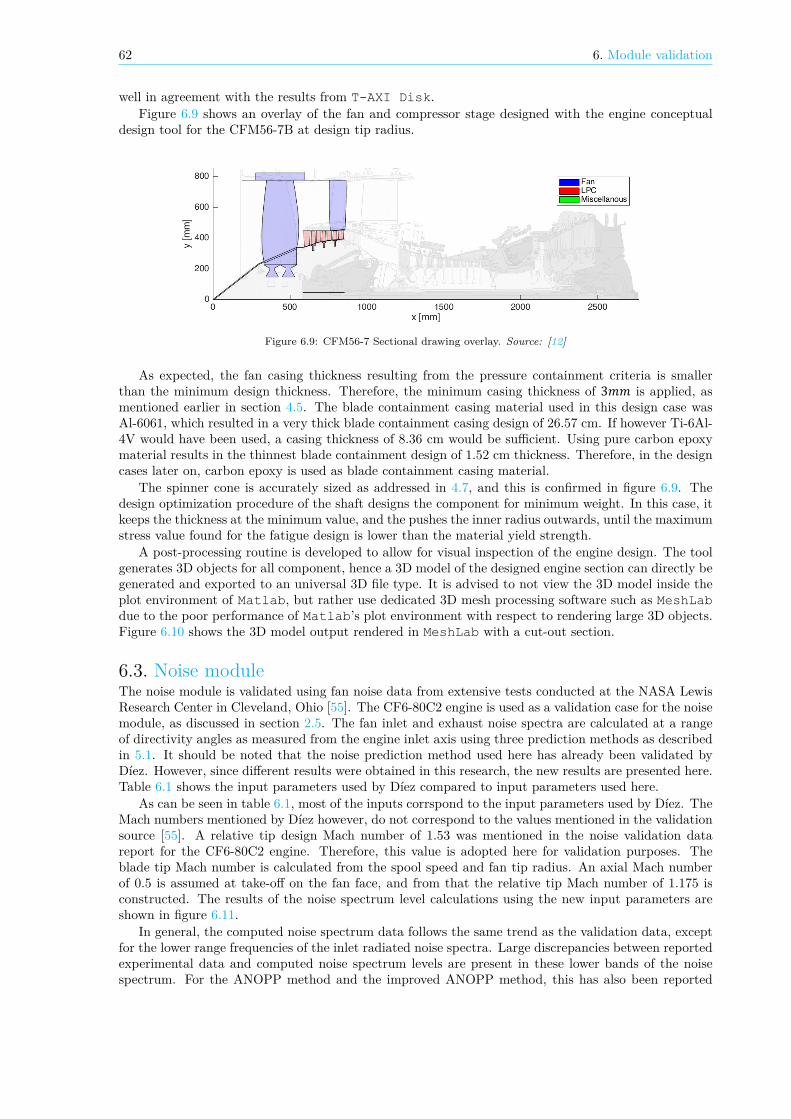
62 6. Module validation
well in agreement with the results from T-AXI Disk.Figure 6.9 shows an overlay of the fan and compressor stage designed with the engine conceptual
design tool for the CFM56-7B at design tip radius.
Figure 6.9: CFM56-7 Sectional drawing overlay. Source: [12]
As expected, the fan casing thickness resulting from the pressure containment criteria is smallerthan the minimum design thickness. Therefore, the minimum casing thickness of 3𝑚𝑚 is applied, asmentioned earlier in section 4.5. The blade containment casing material used in this design case wasAl-6061, which resulted in a very thick blade containment casing design of 26.57 cm. If however Ti-6Al-4V would have been used, a casing thickness of 8.36 cm would be sufficient. Using pure carbon epoxymaterial results in the thinnest blade containment design of 1.52 cm thickness. Therefore, in the designcases later on, carbon epoxy is used as blade containment casing material.
The spinner cone is accurately sized as addressed in 4.7, and this is confirmed in figure 6.9. Thedesign optimization procedure of the shaft designs the component for minimum weight. In this case, itkeeps the thickness at the minimum value, and the pushes the inner radius outwards, until the maximumstress value found for the fatigue design is lower than the material yield strength.
A post-processing routine is developed to allow for visual inspection of the engine design. The toolgenerates 3D objects for all component, hence a 3D model of the designed engine section can directly begenerated and exported to an universal 3D file type. It is advised to not view the 3D model inside theplot environment of Matlab, but rather use dedicated 3D mesh processing software such as MeshLabdue to the poor performance of Matlab’s plot environment with respect to rendering large 3D objects.Figure 6.10 shows the 3D model output rendered in MeshLab with a cut-out section.
6.3. Noise moduleThe noise module is validated using fan noise data from extensive tests conducted at the NASA LewisResearch Center in Cleveland, Ohio [55]. The CF6-80C2 engine is used as a validation case for the noisemodule, as discussed in section 2.5. The fan inlet and exhaust noise spectra are calculated at a rangeof directivity angles as measured from the engine inlet axis using three prediction methods as describedin 5.1. It should be noted that the noise prediction method used here has already been validated byDíez. However, since different results were obtained in this research, the new results are presented here.Table 6.1 shows the input parameters used by Díez compared to input parameters used here.
As can be seen in table 6.1, most of the inputs corrspond to the input parameters used by Díez. TheMach numbers mentioned by Díez however, do not correspond to the values mentioned in the validationsource [55]. A relative tip design Mach number of 1.53 was mentioned in the noise validation datareport for the CF6-80C2 engine. Therefore, this value is adopted here for validation purposes. Theblade tip Mach number is calculated from the spool speed and fan tip radius. An axial Mach numberof 0.5 is assumed at take-off on the fan face, and from that the relative tip Mach number of 1.175 isconstructed. The results of the noise spectrum level calculations using the new input parameters areshown in figure 6.11.
In general, the computed noise spectrum data follows the same trend as the validation data, exceptfor the lower range frequencies of the inlet radiated noise spectra. Large discrepancies between reportedexperimental data and computed noise spectrum levels are present in these lower bands of the noisespectrum. For the ANOPP method and the improved ANOPP method, this has also been reported

6.3. Noise module 63
Figure 6.10: CFM56-7 LPC componenents exported to 3D output.
Table 6.1: Input for noise spectrum level calculations of the CF6-80C2 engine.
Parameter Symbol Input data UnitsNew DíezFan tip radius 𝑟 1.097 1.097 𝑚Temperature increase Δ𝑇 58.66 58.66 𝐾Mass flow rate 802 802 𝑘𝑔/𝑠Spool speed, inlet 𝑁 3150 3150 𝑅𝑃𝑀Spool speed, exhaust 𝑁 3534 3534 𝑅𝑃𝑀Rotor-stator spacing 𝑅𝑆𝑆 200 200 %Rotor blades 𝐵 38 38 −Stator blades 𝑉 80 80 −Design rel. tip Mach number 𝑀 1.53 1.15 −Rel. tip Mach number 𝑀 1.175 1.06 −Blade tip Mach number 𝑀 1.064 0.77 −Measurement radius 𝑟 45.72 45.72 𝑚Measurement angle inlet 𝜃 [20; 50; 80] [20; 50; 80] 𝑑𝑒𝑔Measurement angle exhaust 𝜃 [90; 120; 150] [90; 120; 150] 𝑑𝑒𝑔
by Kontos [55]. Since the ESDU method is based on the same fundamental equations for the noiseprediction, a similar trend is seen here. However, the noise levels for these frequencies are relatively lowas compared to the noise levels at frequencies from 1 kHz and above. Therefore, the error in the lowerrange frequencies will have small impact on the perceivable noise levels.
Another notable detail are the repeating large peaks predicted in sound pressure levels occuringbetween 200 Hz and 6300 Hz using Heidmann’s and improved Heidmann’s methods. These peaks arealso present for the ESDU method, but much more subtle, and correspond well with the data. The peaksare related to the bypass frequency tone, which for the CF6-80C2 at take-off conditions is calculated tobe 𝑓 = 1995𝐻𝑧. Comparing the results to the reported values by Díez [5] and Kontos [55], the effectof the bypass frequency is overestimated here. Since the ESDU method does not suffer from the sameover-predictions, the error is suspected to be caused by the correction factors applied in Heidmann’sand Heidmann’s improved method.

64 6. Module validation
50 100 200 400 800 1600 3150 630020
40
60
80
100
120
1/3- Octave Band Central Frequency [Hz]
SPL
[dB]
Heidmann’s MethodImproved HeidmannESDU MethodExperimental results
(a) Inlet, measured at 20°
50 100 200 400 800 1600 3150 630020
40
60
80
100
1/3- Octave Band Central Frequency [Hz]
SPL
[dB]
Heidmann’s MethodImproved HeidmannESDU MethodExperimental results
(b) Exhaust, measured at 90°
50 100 200 400 800 1600 3150 630020
40
60
80
100
120
1/3- Octave Band Central Frequency [Hz]
SPL
[dB]
Heidmann’s MethodImproved HeidmannESDU MethodExperimental results
(c) Inlet, measured at 50°
50 100 200 400 800 1600 3150 630020
40
60
80
100
1/3- Octave Band Central Frequency [Hz]
SPL
[dB]
Heidmann’s MethodImproved HeidmannESDU MethodExperimental results
(d) Exhaust, measured at 120°
50 100 200 400 800 1600 3150 6300
20
40
60
80
100
1/3- Octave Band Central Frequency [Hz]
SPL
[dB]
Heidmann’s MethodImproved HeidmannESDU MethodExperimental results
(e) Inlet, measured at 80°
50 100 200 400 800 1600 3150 6300
20
40
60
80
100
1/3- Octave Band Central Frequency [Hz]
SPL
[dB]
Heidmann’s MethodImproved HeidmannESDU MethodExperimental results
(f) Exhaust, measured at 150°
Figure 6.11: Fan inlet and exhaust noise spectral comparison of different noise prediction methods for a range ofdirectivity angles measured from engine inlet axis at a 150 (45.27 ) radius.
6.3. Noise module 65
The fly-over procedure is validated using the CFM56-7B engine certification measurement data[13, 105]. The computed equivalent perceived noise level (EPNL) values for the fly-over and lateralnoise measurement points, as described in section 5.5, are shown in figures 6.12 and 6.13 respectively.
From figure 6.12 it can be seen that for the fly-over measurement, the equivalent perceived noiselevel is accurately predicted by the ESDU method. The other two methods over-predict the EPNL.This trend is expected as the flyover simulation is highly dependent on the inlet radiated noise levels.Since both Heidmann’s and improved Heidmann’s method over-predicted the noise spectrum levels, theresults as shown here for the fly-over are as expected. However, from figure 6.13 it can be seen thatfor the lateral noise measurement point, Heidmann’s and the improved Heidmann’s method seem topredict the value most accurate, while the ESDU method predicts a lower value of 86.1 dB.
It is concluded that the fly-over simulation gives a reasonable approximation of the equivalentperceived noise levels as perceived by an observer on the ground. For the computation of the EPNL,the ESDU method will be used for flyover simulations, and Heidmann’s method for the computation ofthe lateral noise measurement.
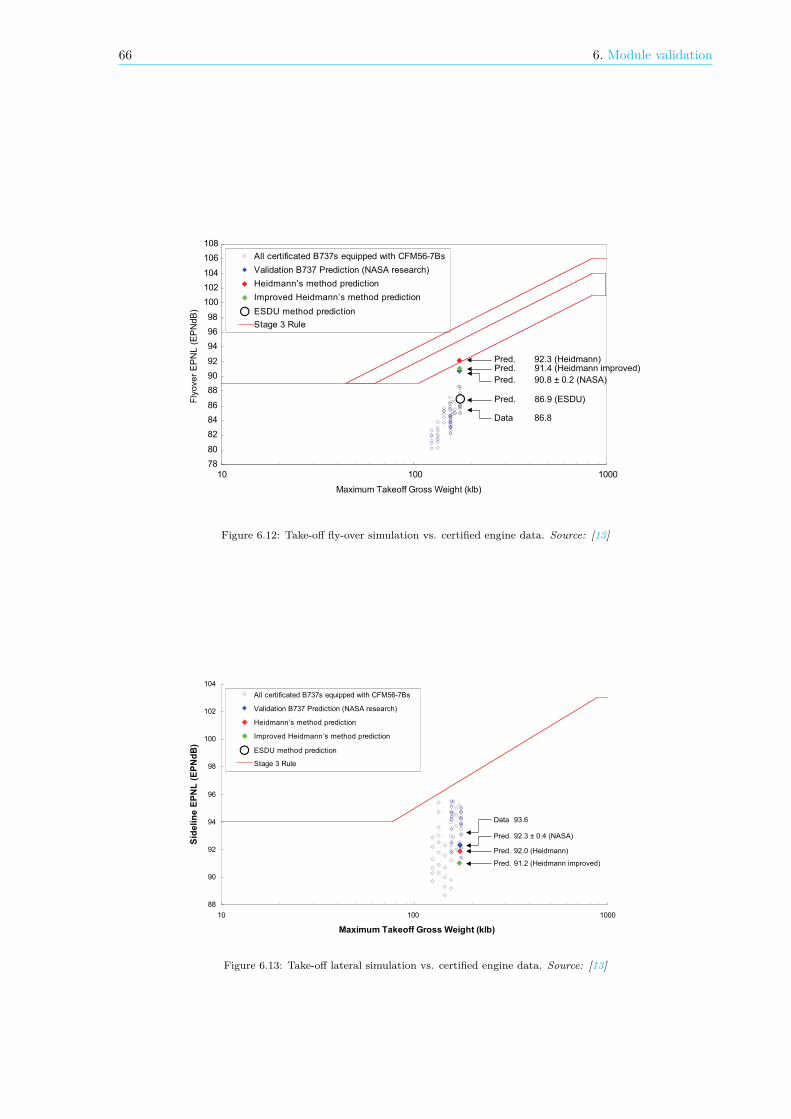
66 6. Module validation
78
80
82
84
86
88
90
92
94
96
98
100
102
104
106
108
10 1000100
Maximum Takeoff Gross Weight (klb)
Fly
ove
r E
PN
L (
EP
Nd
B)
All certificated B737s equipped with CFM56-7Bs
Validation B737 Prediction (NASA research)
Stage 3 Rule
Pred. 90.8 ± 0.2 (NASA)
Data 86.8
Heidmann’s method prediction
Improved Heidmann’s method prediction
ESDU method prediction
Pred. 92.3 (Heidmann)Pred. 91.4 (Heidmann improved)
Pred. 86.9 (ESDU)
Figure 6.12: Take-off fly-over simulation vs. certified engine data. Source: [13]
88
90
92
94
96
98
100
102
104
10 1000
All certificated B737s equipped with CFM56-7Bs
Validation B737 Prediction (NASA research)
Stage 3 Rule
Heidmann’s method prediction
Improved Heidmann’s method prediction
ESDU method prediction
Sid
eli
ne
EP
NL
(E
PN
dB
)
Pred. 92.3 ± 0.4 (NASA)
Data 93.6
100
Maximum Takeoff Gross Weight (klb)
Pred. 92.0 (Heidmann)
Pred. 91.2 (Heidmann improved)
Figure 6.13: Take-off lateral simulation vs. certified engine data. Source: [13]
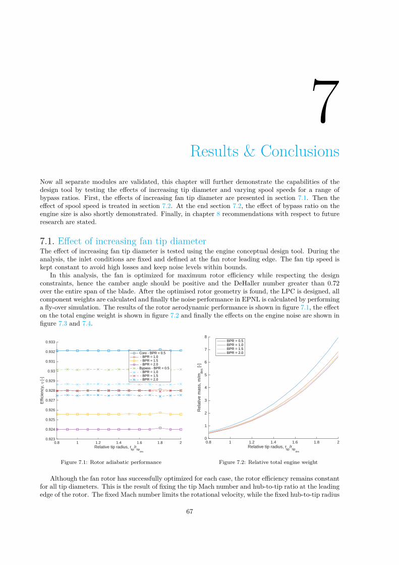
7Results & Conclusions
Now all separate modules are validated, this chapter will further demonstrate the capabilities of thedesign tool by testing the effects of increasing tip diameter and varying spool speeds for a range ofbypass ratios. First, the effects of increasing fan tip diameter are presented in section 7.1. Then theeffect of spool speed is treated in section 7.2. At the end section 7.2, the effect of bypass ratio on theengine size is also shortly demonstrated. Finally, in chapter 8 recommendations with respect to futureresearch are stated.
7.1. Effect of increasing fan tip diameterThe effect of increasing fan tip diameter is tested using the engine conceptual design tool. During theanalysis, the inlet conditions are fixed and defined at the fan rotor leading edge. The fan tip speed iskept constant to avoid high losses and keep noise levels within bounds.
In this analysis, the fan is optimized for maximum rotor efficiency while respecting the designconstraints, hence the camber angle should be positive and the DeHaller number greater than 0.72over the entire span of the blade. After the optimised rotor geometry is found, the LPC is designed, allcomponent weights are calculated and finally the noise performance in EPNL is calculated by performinga fly-over simulation. The results of the rotor aerodynamic performance is shown in figure 7.1, the effecton the total engine weight is shown in figure 7.2 and finally the effects on the engine noise are shown infigure 7.3 and 7.4.
0.8 1 1.2 1.4 1.6 1.8 2Relative tip radius, r
tip/r
tipdes
0.923
0.924
0.925
0.926
0.927
0.928
0.929
0.93
0.931
0.932
0.933
Effi
cien
cy, η
[-]
Core - BPR = 0.5 - BPR = 1.0 - BPR = 1.5 - BPR = 2.0Bypass - BPR = 0.5 - BPR = 1.0 - BPR = 1.5 - BPR = 2.0
Figure 7.1: Rotor adiabatic performance
0.8 1 1.2 1.4 1.6 1.8 2Relative tip radius, r
tip/r
tipdes
0
1
2
3
4
5
6
7
8
Rel
ativ
e m
ass,
m/m
des [-
]
BPR = 0.5BPR = 1.0BPR = 1.5BPR = 2.0
Figure 7.2: Relative total engine weight
Although the fan rotor has successfully optimized for each case, the rotor efficiency remains constantfor all tip diameters. This is the result of fixing the tip Mach number and hub-to-tip ratio at the leadingedge of the rotor. The fixed Mach number limits the rotational velocity, while the fixed hub-to-tip radius
67
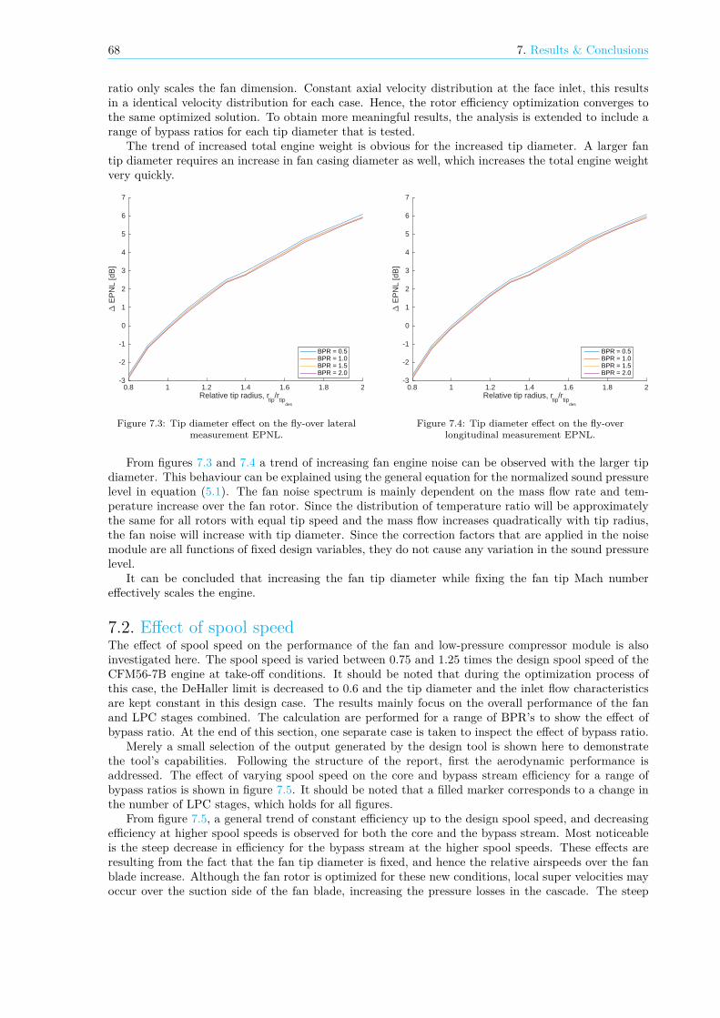
68 7. Results & Conclusions
ratio only scales the fan dimension. Constant axial velocity distribution at the face inlet, this resultsin a identical velocity distribution for each case. Hence, the rotor efficiency optimization converges tothe same optimized solution. To obtain more meaningful results, the analysis is extended to include arange of bypass ratios for each tip diameter that is tested.
The trend of increased total engine weight is obvious for the increased tip diameter. A larger fantip diameter requires an increase in fan casing diameter as well, which increases the total engine weightvery quickly.
0.8 1 1.2 1.4 1.6 1.8 2Relative tip radius, r
tip/r
tipdes
-3
-2
-1
0
1
2
3
4
5
6
7
∆ E
PN
L [d
B]
BPR = 0.5BPR = 1.0BPR = 1.5BPR = 2.0
Figure 7.3: Tip diameter effect on the fly-over lateralmeasurement EPNL.
0.8 1 1.2 1.4 1.6 1.8 2Relative tip radius, r
tip/r
tipdes
-3
-2
-1
0
1
2
3
4
5
6
7
∆ E
PN
L [d
B]
BPR = 0.5BPR = 1.0BPR = 1.5BPR = 2.0
Figure 7.4: Tip diameter effect on the fly-overlongitudinal measurement EPNL.
From figures 7.3 and 7.4 a trend of increasing fan engine noise can be observed with the larger tipdiameter. This behaviour can be explained using the general equation for the normalized sound pressurelevel in equation (5.1). The fan noise spectrum is mainly dependent on the mass flow rate and tem-perature increase over the fan rotor. Since the distribution of temperature ratio will be approximatelythe same for all rotors with equal tip speed and the mass flow increases quadratically with tip radius,the fan noise will increase with tip diameter. Since the correction factors that are applied in the noisemodule are all functions of fixed design variables, they do not cause any variation in the sound pressurelevel.
It can be concluded that increasing the fan tip diameter while fixing the fan tip Mach numbereffectively scales the engine.
7.2. Effect of spool speedThe effect of spool speed on the performance of the fan and low-pressure compressor module is alsoinvestigated here. The spool speed is varied between 0.75 and 1.25 times the design spool speed of theCFM56-7B engine at take-off conditions. It should be noted that during the optimization process ofthis case, the DeHaller limit is decreased to 0.6 and the tip diameter and the inlet flow characteristicsare kept constant in this design case. The results mainly focus on the overall performance of the fanand LPC stages combined. The calculation are performed for a range of BPR’s to show the effect ofbypass ratio. At the end of this section, one separate case is taken to inspect the effect of bypass ratio.
Merely a small selection of the output generated by the design tool is shown here to demonstratethe tool’s capabilities. Following the structure of the report, first the aerodynamic performance isaddressed. The effect of varying spool speed on the core and bypass stream efficiency for a range ofbypass ratios is shown in figure 7.5. It should be noted that a filled marker corresponds to a change inthe number of LPC stages, which holds for all figures.
From figure 7.5, a general trend of constant efficiency up to the design spool speed, and decreasingefficiency at higher spool speeds is observed for both the core and the bypass stream. Most noticeableis the steep decrease in efficiency for the bypass stream at the higher spool speeds. These effects areresulting from the fact that the fan tip diameter is fixed, and hence the relative airspeeds over the fanblade increase. Although the fan rotor is optimized for these new conditions, local super velocities mayoccur over the suction side of the fan blade, increasing the pressure losses in the cascade. The steep

7.2. Effect of spool speed 69
0.75 0.8 0.85 0.9 0.95 1 1.05 1.1 1.15 1.2 1.250.84
0.86
0.88
0.9
0.92
0.94
0.96
Spool speed, RPM/RPMdes
Effici
ency
,𝜂[-]
Core - BPR = 0.5- BPR = 1.0- BPR = 1.5- BPR = 2.0Bypass - BPR = 0.5- BPR = 1.0- BPR = 1.5- BPR = 2.0
Figure 7.5: The effect of spool speed on the bypass and core adiabatic efficiency for a range of bypass ratios.
decrease in efficiency at higher spool speed is resulting from the increasing area of the fan blade that isoperating in the sonic regime, and hence experiences increased shock losses.
The effects of spool speed on the total mass of the entire module is shown in figure 7.8, again for arange of bypass ratios.
0.75 0.8 0.85 0.9 0.95 1 1.05 1.1 1.15 1.2 1.25
400
500
600
700
Spool speed, RPM/RPMdes
Mas
s,m
[kg]
BPR = 0.5BPR = 1.0BPR = 1.5BPR = 2.0
Figure 7.6: Effect of spool speed on total mass for a range of bypass ratios.
Figure 7.8b shows a gradual increase of the compressor weight until the point where a stage canbe removed. The LPC mass then drops, and again starts gradually increasing with spool speed overthe next few iterations. This increase of the LPC mass is caused by the increasing centrifugal loads forhigher spool speeds. Therefore, the LPC rotor disks increase in size to cope with the higher stresses,which increases the LPC component mass.
For the design bypass ratio case, the component weight break-down is given by figure 7.7. Fromfigures 7.8a and 7.8d it can be seen that the fan weight is not strictly dependent on the total fan length.In the lower range of spool speeds the fan length does seem to have some effect. In the higher spoolspeed region, the fan mass increases due to the increased size of the blade containment casing, which

70 7. Results & Conclusions
0.75 0.8 0.85 0.9 0.95 1 1.05 1.1 1.15 1.2 1.250
100
200
300
400
500
600
Spool speed, RPM/RPMdes
Com
pene
ntm
ass,
m[k
g]
TotalFanLPCMiscellanous
Figure 7.7: Component mass break-down for varying spool speed at design BPR.
takes up a large part of the total fan mass.
0.8 0.9 1 1.1 1.2
350
400
450
500
Spool speed, RPM/RPMdes
Fan
mas
s,m
fan
[kg]
BPR = 0.5BPR = 1.0BPR = 1.5BPR = 2.0
(a) Fan stage mass
0.8 0.9 1 1.1 1.20
100
200
300
400
Spool speed, RPM/RPMdes
LPC
mas
s,m
LPC
[kg]
(b) Low-pressure compressor mass
0.8 0.9 1 1.1 1.2
4.4
4.6
4.8
5
5.2
Spool speed, RPM/RPMdes
Misc
ella
neou
sm
ass,
mm
isc
[kg]
(c) Miscellaneous component mass
0.8 0.9 1 1.1 1.20.4
0.6
0.8
1
Spool speed, RPM/RPMdes
Fan
leng
th,L
fan
[m]
(d) Total fan length
Figure 7.8: Effect of spool speed on the aerodynamic efficiency and component mass.
Finally, from the results obtained above, a test case is selected to demonstrate the effect of bypass

7.2. Effect of spool speed 71
ratio on the flow path geometry. In figure 7.6, the spacing between the bypass ratio lines at the designspool speed seems to give a good representation of the average bypass effect. Therefore, the design spoolspeed is taken as case study for bypass ratio effect. Figure 7.9 shows the resulting flow path geometryfor the four bypass ratios considered.
(a) Flowpath geometry at . (b) Flowpath geometry at .
(c) Flowpath geometry at . (d) Flowpath geometry at .
Figure 7.9: Effect of bypass ratio on the flow path geometry and component mass sizes at design spool speed.
As can be seen in figure 7.9a, the total fan length increases with lower bypass ratios. Although fewerLPC stages are required to achieve the desired total core pressure ratio, the LPC stage total length hasincreased since the blades are larger. Furthermore, the fan casing is extended at least up to the endof the compressor, since the weight carrying structure is located behind the rotative part of the LPC.This explains the trend of increasing fan length as seen in figure 7.8d.
To conclude, the increasing tip diameter effectively scales the engine, while the spool speed increasesengine mass and decreases efficiency. The design and sizing tool can be applied to many design cases.The results shown here are just an example of the total output of the tool. More in-depth informationon the separate components is also available from the output, but is not considered here.

8Recommendations
In this chapter the points of improvement to the current work are treated, and areas that need furtherresearch are indicated. First some general recommendations regarding future work on this thesis topicare stated. Thereafter, recommendations are presented consistent to the structure of the report andcode, and hence are treated per module.
In general, the ultimate goal of the thesis subject is arriving at a complete conceptual engine designand sizing tool. Several conceptual engine design and sizing thesis topics have been completed overthe year, such as the conceptual study of contra rotating fans by Díez [5], and Boorsma’s [19] work onthe conceptual design of aeroengine gas generators, and this thesis on the conceptual design and sizingof the fan and low-pressure compressor. Design tools for the low pressure turbine and miscellaneousparts, such as interconnecting ducts between separate components and weight carrying structures, arestill to be developed. To arrive at one single engine design and sizing tool, these separate tools shouldultimately be combined.
Since the number of design variables in the engine design process is quite large and proper sharingof information between modules in the process is critical, the total engine design tool needs to be wellstructured. To ensure integration of the separate design tools is possible in the end, a recommendationwould be to dedicate one research topic to the development of one proper structured module-basedengine design tool. All currently developed design tools should be thoroughly analysed and updatedwhere necessary to comply to the base module format, using one coding style format in the end.
8.1. Aerodynamics module• In the LPC design module, include falling mean-line design without a fixed hub diameter for more
realistic LPC modelling.
• Include a simplified equation of state model. The speed performance of the current high-levelintegrated Matlab interface of the CoolProp software is slowing down iterative solving process,due to numerous function calls in the conversion loop. Either the low-level DLL interaction couldbe used to speed up the calculation process, or the use of simplified equations of state dedicatedto air gas property calculations could increase speed.
• Include design of nozzles and fan cowling.
8.2. Structural & analysis module• More detailed design of fan casing, as it makes up for a large portion of the total engine weight.
• Use ribbed blade containment casing design and include structural analysis of such geometry.
• Include design and sizing of load carrying structure of the engine.
• Include calculations of blade stresses.
• Include basic vibration analysis for blades and disks.
73
74 8. Recommendations
8.3. Noise module• Revision of the noise module. It was assumed that the noise module was readily available and fully
functional. However, validation and application on design cases showed that the noise moduleshows inaccurate results. Further research is needed to inspect if this is a failure of the codeor the wrong implementation here. Quick inspection of the design code however showed severalerrors, for example not considering the absolute value of the the cut-off correction factor 𝛿, andthe absence of some correction factor at the broad-band noise calculation at subsonic relativedesign tip Mach number. Due to time constraints a full revision of the code was not carried outhere, but it is advised to look further into this.
• Vectorize the noise module for increased speed performance. This will prove especially useful whenused inside an optimization routine. Since the noise prediction method output is non-linear andcontains logical statements, a global optimization routine such as a genetic algorithm or a patternsearch should be used for optimization purposes. These methods often have a high number offunction evaluations before reaching a global optimum, and therefore speed increase of the codeis an important criteria.
• Include other flight simulations such as landing approach and include thrust cut-back profiles.
• Inclusion of atmospheric attenuation effects in the perceived noise level calculations, as mentionedby Díez [5].
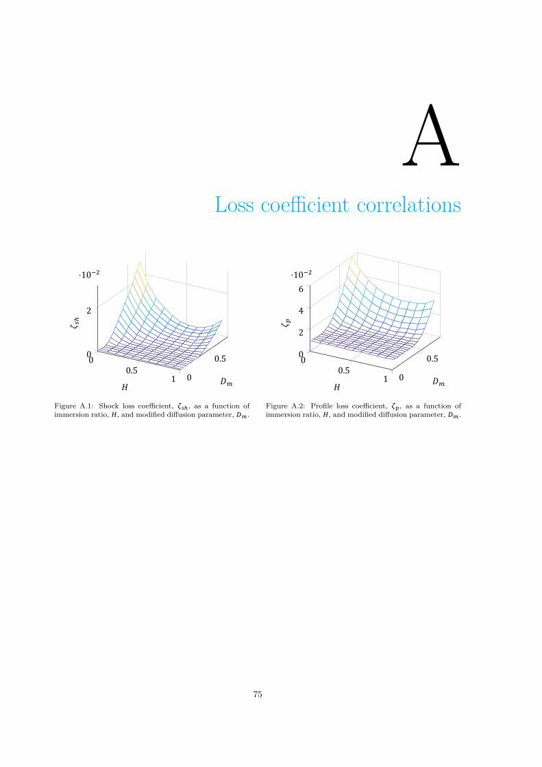
ALoss coefficient correlations
00.5
1 0
0.50
2
⋅10
𝐻 𝐷
𝜁
Figure A.1: Shock loss coefficient, , as a function ofimmersion ratio, , and modified diffusion parameter, .
00.5
1 0
0.50
2
4
6⋅10
𝐻 𝐷
𝜁
Figure A.2: Profile loss coefficient, , as a function ofimmersion ratio, , and modified diffusion parameter, .
75


Bibliography[1] IATA, German Aerospace Center (DLR), and Georgia Institute of Technology, IATA Technology
Roadmap 2013, (2013).
[2] General Electric, CF6-80C2 Airflows FADEC Control - Information poster C1010-FAD1, .
[3] L. R. Jenkinson, J. F. Marchman, L. Jenkinson, and J. Marchman, Aircraft Design Projects(Butterworth-Heinemann, 2003) p. 392.
[4] C. Soares, Gas Turbines: A Handbook of Air, Land and Sea Applications, 2nd ed. (Elsevier Inc.,Oxford, UK, 2014).
[5] N. G. Díez and d. A. G. Rao, Faculty of Aerospace Engineering, Tech. Rep. (Delft University ofTechnology, Delft, 2009).
[6] S. Farokhi, Aircraft propulsion, 2nd ed. (Wiley Publishing, Inc., Chichester, U.K., 1971) p. 1048.
[7] M. Schobeiri, Turbomachinery Flow Physics and Dynamic Performance (Springer Berlin Heidel-berg, Berlin, Heidelberg, 2005) pp. 1–522.
[8] N. Falck, Axial Flow Compressor Mean Line Design, Msc thesis, Lund University, Sweden (2008).
[9] Y. Lee, J. Pan, R. Hathaway, and M. Barkey, Fatigue Testing and Analysis (Elsevier Inc., Oxford,UK, 2005) p. 417.
[10] J. Kurzke, GasTurb Details GasTurb Details 5, (2007).
[11] M. T. Tong, I. Halliwell, and L. J. Ghosn, A Computer Code for Gas Turbine Engine Weight andDisk Life Estimation, Journal of Engineering for Gas Turbines and Power 126, 265 (2004).
[12] CFM International, Training Manual CFM56-6B (Basic Engine), January (CFM International,Melun Cedex, France, 1998).
[13] M. D. Dahl, Overview of Aircraft Noise Prediction Tools Assessment, Tech. Rep. (NASA, Cleve-land, OH, 2007).
[14] J. Kurzke, VKI LS 2013-04: Aeroengine design: From state of the art of turbofans towardsinnovatove architectures, Lecture series / Von Karman Institute for Fluid Dynamics (KarmanInstitute for Fluid Dynamics, 2013) Chap. 1.
[15] K. Kyprianidis, Multi-disciplinary conceptual design of future jet engine systems, Ph.D. thesis,Cranfield University (2010).
[16] K. Kyprianidis and A. Dax, Low pressure system component advancements and its impact onfuture turbofan engine emissions, in Paper No. ISABE-2009- …, November 2015 (2009) pp. 1–14.
[17] E. Roux, Turbofan and Turbojet Engines: Database Handbook (Élodie Roux, 2007).
[18] S. A. Korpela, Principles of Turbomachinery, 1st ed. (John Wiley & Sons, Inc., Hoboken, NewJersey, 2011) p. 476.
[19] M. J. Boorsma and d. A. G. Rao, Faculty of Aerospace Engineering, Tech. Rep. (Delft Universityof Technology, Delft, 2015).
[20] R. Boyer, G. Welsch, and E. W. Collings, ASM Materials Properties Handbook: Titanium Alloys(ASM lnternatlonal, Materials Park, OH, 1994) p. 1176.
77

78 Bibliography
[21] R. L. Dreshfield, Long Time Creep Rupture of Haynes(TM) Alloy 188, Tech. Rep. (NASA, Cleve-land, Ohio, 1996).
[22] Airbus GMF, Global Market Forecast 2015, (2015).
[23] ACARE Strategy Review Group, Aeronautics and Air Transport: Beyound Vision 2020 (Towards2050), Tech. Rep. (Advisory Council for Aeronautics Research in Europe (ACARE), Brussels,2010).
[24] High Level Group on Aviation Research, Flightpath 2050, (2011).
[25] Air Transport Action Group, A sustainable flightpath towards reducing emissions, (2012).
[26] T. Obrecht, Aeroengine Design: From State of the Art of Turbofans Towards Innovative Archi-tectures, Lecture series / Von Karman Institute for Fluid Dynamics (Karman Institute for FluidDynamics, 2013) Chap. 3.
[27] N. Smith, Aeroengine Design: From State of the Art of Turbofans Towards Innovative Archi-tectures, Lecture series / Von Karman Institute for Fluid Dynamics (Karman Institute for FluidDynamics, 2013) Chap. 2.
[28] A. Amato, J. Seitzman, and T. Lieuwen, Gas Turbine Emissions, timothy c. ed., edited by T. C.Lieuwen and V. Yang, Vol. 38 (Cambridge University Press, New York, NY, 2013) pp. 209–234.
[29] R. Dénos and G. Paniagua, Aeroengine Design: From State of the Art of Turbofans TowardsInnovative Architectures, Lecture series / Von Karman Institute for Fluid Dynamics (KarmanInstitute for Fluid Dynamics, 2013) Chap. 6.
[30] R. Dénos and G. Paniagua, Aeroengine Design: From State of the Art of Turbofans TowardsInnovative Architectures, Lecture series / Von Karman Institute for Fluid Dynamics (KarmanInstitute for Fluid Dynamics, 2013) Chap. 7.
[31] J. D. Mattingly, Aircraft Engine Design, 2nd ed. (American Institute of Aeronautics and Astro-nautics, Inc., Reston, VA, 2002).
[32] R. W. Koenig and L. H. Fishbach, GENENG — A Program For Calculating Design and Off-DesignPerformance for Turbojet and Turbofan Engines, Tech. Rep. February (NASA, Washington D.C.,1972).
[33] L. H. Fishbach and R. W. Koenig, GENENG II — A Program for Calclating Design and Off-Design Performance of Two- and Three-Spool Turbofans With As Many As Three Nozzles, Tech.Rep. February (NADA, Washington D.C., 1972).
[34] W. L. MacMillan and J. Palmer, Development of a Modular Type Computer Program for theCalculation of Gas Turbine Off Design Performance, Tech. Rep. (Cranfield Institure of Technology,Cranfield, UK, 1974).
[35] J. R. Palmer and Y. Cheng-zhong, TURBOTRANS: a Programming Language for the Perfor-mance Simulation of Arbitrary Gas Turbine Engines with Arbitrary Control Systems, in ASME1982 International Gas Turbine Conference and Exhibit, Vol. 5 (American Society of MechanicalEngineers, London, UK, 1982) p. 8.
[36] W. P. J. Visser, Gas Turbine Engine Simulation At NLR, in CEAS Symposium on SimulationTechnology, ”Making it Real” (Delft, 1995).
[37] W. P. J. Visser and M. J. Broomhead, GSP — A Generic Object-Oriented Gas Turbine SimulationEnvironment, Tech. Rep. (National Aerospace Laborator (NLR), 2000).
[38] T. Grönstedt, Development of Methods for Analysis and Optimization of Complex Jet EngineSystems, Ph.D. thesis, Chalmers University of Technology (2000).
Bibliography 79
[39] U. T. J. Grönstedt and P. Pilidis, Control Optimization of the Transient Performance of theSelective Bleed Variable Cycle Engine During Mode Transition, Journal of Engineering for GasTurbines and Power 124, 75 (2002).
[40] R. W. Claus, A. L. Evans, J. K. Lylte, and L. D. Nichols, Numerical Propulsion System Simula-tion, Computing Systems in Engineering 2, 357 (1991).
[41] C. K. Drummond, G. J. Follen, and C. W. Putt, Gas Turbine System Simulation: An Object-Oriented Approach, Tech. Rep. (National Aeronautics and Space Administration (NASA), Cleve-land, Ohio, 1992).
[42] J. K. Lytle, The Numerical Propulsion System Simulation: An Overview, CAS 2000 Work-shop/The Ames Research Center (2000).
[43] A. Alexiou, E. H. Baalbergen, O. Kogenhop, K. Mathioudakis, and P. Arendsen, AdvancedCapabilities for Gas Turbine Engine Performance Simulations, in Volume 1: Turbo Expo 2007(ASME, 2007) pp. 19–28.
[44] A. Bala, V. Sethi, E. L. Gatto, V. Pachidis, and P. Pilidis, PROOSIS – A Collaborative Venturefor Gas Turbine Performance Simulation using an Object Oriented Programming Schema, Power(2007).
[45] P. Lolis, Development of a Preliminary Weight Estimation Method for Advanced Turbofan Engines,Phd, Cranfield University (2014).
[46] D. a. Sagerser, S. Lieblein, R. P. Kkebs, N. Aeronautics, and T. Memorandum, Emperical Ex-pressions for Estimating Length and Weight of Axial-Flow Components of VTOL Powerplants,Tech. Rep. (NASA, Washington D.C., 1971).
[47] R. Pera, E. Onat, G. Klees, and E. Tjonneland, A Method to Estimate Weight and Dimensions ofAircraft Gas Turbine Engines. Volume 1: Method of Analysis, Tech. Rep. (NASA, Seattle, WA,1977).
[48] G. W. Klees and L. H. Fishbach, Aircraft Engine Weight Estimation Method, in 37th AnnualConference, Munich, West Germany, May 8-10, Society of Allied Weight Engineers, Inc. (Societyof Allied Weight Engineers, Inc., Munich, West Germany, 1978) p. 28.
[49] E. Onat and G. Klees, A Method to Estimate Weight and Dimensions of Large and Small GasTurbine Engines, Tech. Rep. (NASA, Seattle, WA, 1979).
[50] P. L. Hale, A Method to Estimate Weight and Dimensions of Small Aircraft Propulsion GasTurbine Engines, Tech. Rep. (NASA, Phoenix, Arizona, 1982).
[51] V. Sanghi, S. K. Kumar, S. K. Sane, and V. Sundararajan, Preliminary Estimation of EngineGas-Flow-Path Size and Weight, Journal of Propulsion and Power 14, 208 (1998).
[52] M. T. Tong and B. a. Naylor, An Object-Oriented Computer Code for Aircraft Engine WeightEstimation, Volume 1: Aircraft Engine; Ceramics; Coal, Biomass and Alternative Fuels; Manu-facturing, Materials and Metallurgy; Microturbines and Small Turbomachinery , 1 (2008).
[53] S. Bretschneider, O. Arago, and S. Staudacher, Architecture of a Techno and Environmental RiskAssessment Tool Using a Multi-Modular Build Approach, in ISABE 2007 Proceedings (2007) p.1103.
[54] M. F. Heidmann, Interim Prediction Method for Fan and Compressor Source Noise, NASA Sci-entific and Technical Information Branch (1979).
[55] K. B. Kontos, R. E. Kraft, and P. R. Gliebe, Improved NASA-ANOPP Noise Prediction ComputerCode for Advanced Subsonic Propulsion Systems, Tech. Rep. 24 (NASA, Cincinnati, Ohio, 1996).
[56] J. R. Stone, E. A. Krejsa, and B. J. Clark, Jet Noise Modeling for Coannular Nozzles Includingthe Effects of Chevrons, National Aeronautics and Space Administration (2003).

80 Bibliography
[57] Society of Automotive Engineers, Gas Turbine Jet Exhaust Noise Prediction, Aerospace recom-mended practice (Society of Automotive Engineering, 1994) p. 114.
[58] E. A. Krejsa and M. F. Valerino, Interim Prediction Method for Turbine Noise, Tech. Rep. (NASA,Cleveland, Ohio, 1976).
[59] M. Fink, Airframe Noise Prediction Method, Tech. Rep. (U.S. Department of Transportation,Washington D.C., 1977).
[60] SAE. Comitee A-21, Aircraft Noise., Standard values of atmospheric absorption as a function oftemperature and humidity, Tech. Rep. (Society of Automotive Engineers, 1975).
[61] C. Chien and W. Soroka, Sound propagation along an impedance plane, Journal of Sound andVibration 43, 9 (1975).
[62] SAE – Comitee A-21, Aircraft Noise., Prediction Method of Lateral Attenuation of Airplane NoiseDuring Takeoff and Landing, Tech. Rep. (Society of Automotive Engineers, 1981).
[63] A. Blackner and T. Bhat, Installation effects on coaxial jet noise - An experimental study, in 36thAIAA Aerospace Sciences Meeting and Exhibit, Vol. 53 (American Institute of Aeronautics andAstronautics, Reston, Virigina, 1998) pp. 1–36, arXiv:arXiv:1011.1669v3 .
[64] D. B. Hanson, Noise of counter-rotation propellers, Journal of Aircraft 22, 609 (1985).
[65] C. E. Whitfield, R. Mani, and P. R. Gliebe, High Speed Turboprop Aeroacoustic Study (Counter-rotation) Volume I - Model Development, Tech. Rep. (NASA, Cincinnati, Ohio, 1992).
[66] S. Dixon and C. Hall, Fluid Mechanics and Thermodynamics of Turbomachinery, 7th ed. (ElsevierInc., Oxford, UK, 1995) p. 536.
[67] J.-M. Tournier and M. S. El-Genk, Axial flow, multi-stage turbine and compressor models, EnergyConversion and Management 51, 16 (2010).
[68] L. Reid and R. D. Moore, Performance of Single-Stage Axial-Flow Transonic Compressor WithRotor and Stator Aspect Ratios of 1.19 and 1.26, Respectively, and With Design Pressure Ratioof 1.82, Tech. Rep. November 1978 (NASA, Cleveland, OH, 1978).
[69] R. D. Moore and L. Reid, Performance of Single-Stage Axial-Flow Transonic Compressor withRotor and Stator Aspect Ratios of 1.63 and 1.78, Respectively, and with Design Pressure Ratio of1.82, Tech. Rep. (NASA, Cleveland, OH, 1982).
[70] R. D. Moore and L. Reid, Performance of Single-Stage Axial-Flow Transonic Compressor WithRotor and Stator Aspect Ratios of 1.19 and 1.26, Respectively, and With Design Pressure Ratioof 2.05, Tech. Rep. (NASA, Cleveland, OH, 1980).
[71] W. M. Osborn and R. J. Steinke, Performance of a 1.15-Pressure-Ratio Axial-Flow Fan Stagewith a Blade Tip Solidity of 0.5, Tech. Rep. (NASA, Cleveland, OH, 1974).
[72] R. D. Moore and R. J. Steinke, Aerodynamic Performance of a 1.25-Pressure-Ratio Axial-FlowFan Stage, Tech. Rep. (NASA, Cleveland, OH, 1974).
[73] W. M. Osborn, R. D. Moore, and R. J. Steinke, Aerodynamic Performance of a 1.35-Pressure-Ratio Axial-Flow Fan Stage, Tech. Rep. (NASA, Cleveland, OH, 1978).
[74] G. W. Lewis, R. D. Moore, and G. Kovich, Performance of a 1.20-Pressure-Ratio STOL FanSTage at Three Rotor Blade Setting Angles, Tech. Rep. NASA TM X-2837 (NASA, 1973).
[75] R. D. Moore and W. M. Osborn, Aerodynamic Performance of 1.38-Pressure-Ratio, Variable-PitchFan Stage, Tech. Rep. (NASA, Cleveland, OH, 1979).
[76] D. C. Urasek, W. T. Gorrell, and W. S. Cunnan, Performance of Two-Stage Fan Having Low-Aspect Ratio, First-Stage Rotor Blading, Tech. Rep. (NASA, Cleveland, OH, 1979).
Bibliography 81
[77] R. H. Aungier, Axial-Flow Compressors (ASME Press, New York, NY, 2003) p. 368.
[78] A. R. Howell, Fluid dynamics of axial compressors, ARCHIVE: Proceedings of the Institution ofMechanical Engineers 1847-1982 (vols 1-196) 153, 441 (1945).
[79] I. Johnsen and R. Bullock, Aerodynamic Design Of Axial-Flow Compressors (NASA Lewis Re-search Center, Cleveland, Ohio, 1965).
[80] S. Lieblein, F. Schwenk, and R. Broderick, Diffusion factor for estimating losses and limitingblade loadings in axial-flow-compressor blade elements, NACA Research Memorandum , 1 (1953).
[81] M. T. Schobeiri, Advanced Compressor Loss Correlations, Part II: Experimental Verifications,Int. J. Rotating Machinery 3, 179 (1997).
[82] M. T. Schobeiri, Advanced Compressor Loss Correlations, Part I: Theoretical Aspects, Int. J.Rotating Machinery 3, 179 (1997).
[83] W. Jansen and W. C. Moffatt, The Off-Design Analysis of Axial-Flow Compressors, Journal ofEngineering for Gas Turbines and Power 89, 453 (1967).
[84] M. Davis, A stage-by-stage dual-spool compression system modeling technique, ASME InternationalGas Turbine Conference and Exhibi , 1 (1982).
[85] W. R. Davis, A computer program for the analysis and design of turbomachinery – Revision, Tech.Rep. (Division of Aerothermodynamics, Carleton University, Ottowa, Canada, 1971).
[86] W. C. Swan, A Practical Method of Predicting Transonic-Compressor Performance, Journal ofEngineering for Power 83, 322 (1961).
[87] L. Aleid, Variable cycle propulsion systems for a supersonic civil transport, , 275 (1997).
[88] S. Lieblein, Loss and Stall Analysis in Compressor Cascades, Journal of Basic Eng. 81, 387 (1959).
[89] C. C. Koch and L. H. Smith, Loss Sources and Magnitudes in Axial-Flow Compressors, Journalof Engineering for Power 98, 411 (1976).
[90] R. H. Aungier, Turbine Aerodynamics: Axial-Flow and Radial-Flow Turbine Design and Analysis(ASME Press, New York, NY, 2005) p. 404.
[91] M. I. Yaras and S. a. Sjolander, Prediction of Tip-Leakage Losses in Axial Turbines, Journal ofTurbomachinery 114, 204 (1992).
[92] F. G. Pascual and W. Q. Meeker, Estimating Fatigue Curves With the Random Fatigue-LimitModel, Technometrics 41, 277 (1999).
[93] S. C. Armand, Structural Optimization Methodology for Rotating Disks of Aircraft Engines, Tech.Rep. November (NASA, Washington D.C., 1995).
[94] D. Gutzwiller, T-Axi Disk V2.2 User ’ s Guide and Tutorial, Ewp.Rpi.Edu , 1 (2009).
[95] D. P. Gutzwiller and M. G. Turner, Rapid low fidelity turbomachinery disk optimization, Advancesin Engineering Software 41, 779 (2010).
[96] M. C. Potter, J. L. Goldberg, and E. Aboufadel, Advanced Engineering Mathematics, 3rd ed.(Oxford University Press, 2005).
[97] A. Mendelson and S. Manson, Practical Solution of Plastic Deformation Problems in Elastic-Plastic Range, Tech. Rep. (NASA, Cleveland, Ohio, 1957).
[98] S. Bretschneider, F. Rothe, M. G. Rose, and S. Staudacher, Compressor Casing PreliminaryDesign Based on Features, in Volume 5: Structures and Dynamics, Parts A and B (ASME, 2008)pp. 1–9.
[99] A. Carman, Resistance of Tubes to Collapse, University of Illinois Bulletin 3 (1906).

82 Bibliography
[100] T. B. Dewhurst, The Impact Load on Containment Rings During a Multiple Blade Shed in AircraftGas Turbine Engines, International Gas Turbine and Aeroengine Congress and Exposition (1991),10.1115/91-GT-163.
[101] ESDU, Prediction of Noise Generated by Fans and Compressors in Turbojet and Turbofan Engines(ESDU International PLC, London, UK, 1998).
[102] M. F. Heidmann and C. E. Feiler, Noise comparisons from full-scale fan tests at NASA LewisResearch Center, Tech. Rep. (NASA Lewis Research Center, Cleveland, OH, 1973).
[103] Boeing Commercial Airplanes, Boeing 767 Airplane Characteristics for Airport Planning, Tech.Rep. (2005).
[104] Federal Aviation Administration, Noise Certification Standards for Subsonic Jet Airplanes andSubsonic Transport Category Large Airplanes, Federal Register 65, 1 (2000).
[105] Federal Aviation Administration, Estimated Airplane Noise Levels in A-Weighted Decibels, Tech.Rep. January (U.S. Department of Transportation, 2012).