News Driven Business Cycles: Insights and Challenges

Paul Beaudry∗ and Franck Portier†‡

February 2014Final version

Forthcoming in the Journal of Economic Litterature

Abstract

There is a widespread belief that changes in expectations may be an importantindependent driver of economic fluctuations. The news view of business cycles offersa formalization of this perspective. In this paper we discuss mechanisms by whichchanges in agents’ information, due to the arrival of news, can cause business cyclefluctuations driven by expectational change, and we review the empirical evidenceaimed at evaluating their relevance. In particular, we highlight how the literature onnews and business cycles offers a coherent way of thinking about aggregate fluctuations,while at the same time we emphasize the many challenges that must be addressed beforea proper assessment of the role of news in business cycles can be established.

Key Words : News, Business Cycles, Expectations, Pigou, Keynes, Recessions

JEL Class. : E3

∗Vancouver School of Economics, University of British Columbia and NBER. (paulbe@mail.ubc.ca)†Toulouse School of Economics and CEPR (Franck.Portier@TSE-fr.eu)‡The authors have benefited from discussion with Fabrice Collard, Martial Dupaigne, Patrick Feve,

Domenico Giannone and Andre Kurmann. They want to thank Dana Galizia for excellent research assistance.Comments of two referees are also gratefully aknowledged.

1

1 Introduction

Why do market economies exhibit business cycle phenomena; that is, why do they exhibit

recurring boom periods with higher than average growth in investment, consumption and

employment, followed by recessions characterized by declines in these same macroeconomic

aggregates? The news view of business cycles suggests that these phenomena are mainly the

result of agents having incentives to continuously anticipate the economy’s future demands. If

an agent can properly anticipate a future need, he can gain by trying to preempt the market

and invest early as to make goods readily available when the predicted needs eventually

appear. If many agents adopt similar behavior, because they receive related news about

future developments, this will lead to a boom period. However, by the very fact that such

behavior involves speculation, it will be subject to errors. In the cases of error, the economy

will have over-invested as the anticipated demand will not materialize. This will cause a

recession and a process of liquidation. Hence, according to the news view of the business

cycle, both the boom and the bust are direct consequences of people’s incentive to speculate

on information related to future developments of the economy.

An interesting anecdotal evidence for such speculative cycles is given by the satellite

industry. In the early 1980s, in anticipation of long-distance telephone service, video tele-

conferencing and other forms of sophisticated electronic communications, the launching of

telecommunication satellites exploded. A couple of years later, the market realized that the

increase in demand failed to materialize, which caused severe capacity underutilization. On

a weekday afternoon in December 1983, the Federal Communications Commission observed

that only 54% of capacity on communications satellites was in use. Of the 14 satellites stud-

ied, 143 of 312 transponders were idle. Six months earlier, before 48 new transponders had

been introduced, 36 fewer were idle and capacity utilization reached 59%. 1 This “transpon-

der glut” repeated in the early 2000s. During the “dot com” boom of the 1990s, prospective

demand for data transmission led the market increase dramatically the number of launched

satellites. In 1998, the satellite industry launched 150 satellites, a nearly 300 percent growth

compared to 1993 (Hague [2003]). It was not a radical change in the launching technol-

ogy that caused such a boom, neither the current demand for data transmission 2, but the

perceived future profitability of satellites operation associated with the development of the

IT economy. With the bust of year 2000, the number of satellites launched went down to

75 in 2001 and 69 in 2003, against 150 in 1998 (OECD [2004]). The sector then went to

a period of liquidation and falling prices. As described by the magazine Satellite News of

1 “Satellites outpace customers”, The New-York Times, April 10, 1984.2The growth rate for demand for satellite bandwidth has been 31% between 1995 and 2003, while the

supply of satellite bandwidth grew by 54% during this same timeframe (Futron Corporation [2004]).

1

Nov 4, 2002, “Companies that purchased satellite transponder capacity during the industry’s

halcyon days are now struggling to resell the capability in the face of falling market prices”.

While the idea of news driven business cycles is rather simple, and echoes commonly

found narratives in the business press, as illustrated above, evaluating its relevance is quite

challenging. Difficulties arise on two main fronts. On the one hand, since the main driving

force is agents’ perceptions about the economy’s future needs, it implies that the business

cycle is driven by a force difficult to measure. This generally makes empirical evaluation

depend on subtle identification assumptions and therefore subject of debate. On the other

hand, even if the underlying story appears intuitive, it turns out that it is quite challeng-

ing to build a simple macroeconomic model which captures in a robust way the idea that

changes in agents’ perceptions about the economy’s future needs can cause business cycle

type fluctuations. In fact, we will show why one generally needs to depart at least from some

standard modeling assumption to be able capture the notion of news driven business cycles

within the confines of a dynamic general equilibrium framework. These two issues, modeling

and evaluating news driven business cycles, will be at the heart of this article. In particular,

the goal of this article will be to highlight both the promising paths and the difficulties in

building and evaluating the news view of business cycles.

The idea of business cycles driven by expectations can be traced back to writing such as

that of Pigou [1927] where he states “The varying expectations of business men ... constitute

the immediate cause and direct causes or antecedents of industrial fluctuations”. According

to Pigou, the very source of fluctuations is the “wave-like swings in the mind of the business

world between errors of optimism and errors of pessimism”. 3 This view is also closely

related to Keynes’ [1936] notion of animal spirits as it relates to these waves of optimism and

pessimism as important driving forces behind economic fluctuations. There are at least three

different ways of interpreting optimism and pessimism in business cycles. At one extreme

is the view that such waves are entirely psychological phenomenon, with no grounding in

economic reality. According to such a perspective, any expansion driven by optimism must

eventually lead to a crash as the expansion is not supported by any change in fundamentals.

At the other extreme is the view that the macro-economy is inherently unstable as it admits

self-fulfilling fluctuations. In this perspective, a wave of optimism creates a boom which

renders the initial optimism rational, and the same is true of waves of pessimism. A third

possibility is the news view whereby agents in the economy are continually trying to predict

future needs, but likely do so imperfectly. In this interpretation, a boom driven by a wave of

optimism arises when agents have gathered information suggesting that future fundamentals

favor high investment demand today. If their information is valid and expectations are

3See Collard [1983] and [1996] on the business cycle theory of Pigou.

2

realized, then the boom needs not be followed by a crash. In contrast, if agents have made

an error and have been overly optimistic, then there will be a crash. This type of recurrent

boom and occasional bust phenomena, driven by information and possible errors, is the

defining property of news-driven business cycles. 4 The empirical evidence we will review in

this survey lead us to favor this third possibility.

One important issue that arises when considering any theory of business cycles is whether

it implies that cycles are efficient or not. While we agree on the relevance of this issue, it

will not be a major focus of this article. At this point in time we see the news view of

business cycles as primarily proposing a positive theory of fluctuations where, depending on

the details, the fluctuations may or may not be efficient. In the literature we will review,

some of the models imply that the resulting cycles are efficient while others imply they are

not. We will point out these differences as they arise.

1.1 Overview

The survey is structured as follows. In Section 2 we begin by presenting the general idea of

news in terms of innovations in agents’ information sets that are useful for predicting future

fundamentals. The fundamentals of interest could be of many of difference sources, but in

much of the applied news literature the fundamental being predicted is productivity. We

emphasize the difference between two information structures, one where the news can be

wrong and one where the news is right but incomplete. The case where the news can be

wrong is generally referred to a the noise formulation. Recognizing the difference between

these two formulations is important when bringing the idea of news to the data.

In Section 2.1 we present a baseline general equilibrium model where booms are driven

by optimistic news which favor current investment, while a bust arises if and when a news is

recognized to be wrong. This baseline model abstracts from many important features, but for

illustrative purposes is very helpful since it offers a closed form solution in which optimistic

news are expansionary, and where revisions can lead to busts. The environment considered

consists of a final good consumption sector produced by intermediate goods. Investment in

each sector depends on the future prices. We allow agents to receive news about the future

productivity in each of the intermediate good sectors. When all the intermediate goods

are substitutable in the production of the final good, we show that only the expectation of

the aggregate level of productivity matters at the symmetric equilibrium for determining

investment . In this case, we can formalize the information process in the following way:

agents receive in period t a noisy signal about aggregate productivity of period t+q. Then in

4The word ‘news” is used here to represent exogenous changes in the information sets that agents use toform their perceptions regarding future economic activity.

3

period t+ q, information is revealed. The arrival of positive news is shown to cause a boom

period as expectations about the future are optimistic, with investment and hours worked

increasing immediately and consumption increasing with a lag. If at t+q productivity growth

meets expectations, which happens on average when agents are Bayesian, then the boom

period continues and the economy converges to its new steady state. If however expectations

are not met because the signal was wrong, then the economy enters a recessionary period

with macroeconomic aggregates going down. We discuss the conditions under which the

economy actually enters a liquidation phase after the misinterpretation of a news shock,

with investment dropping drastically and staying below its steady state on the convergence

path back to the steady state. We then use this basic model to discuss various information

structure and interpretation of the shocks. For example, we examine a case where information

is dispersed and each firm receives a idiosyncratic noisy signal. We show that this problem

exhibits a complementarity structure whereby firms in one sector will want to increase their

production if they expect others to increase their production, regardless of the actual news

received. This baseline model has some undesirable features as consumption responses to

news only with a lag and the real wage is constant. In later sections we discuss more

complicated models which do not have these features. An important feature on this baseline

model is that offers an explicit framework in which the empirical exercises reviewed in Section

3 can be interpreted.

In Section 3 we start by providing some simple reduced form evidence that is suggestive

of the news view of business cycles and then we summarize VAR evidence which has been

presented as both supportive and dismissive of the news view. The reduced-form evidence is

based on the cyclical property of the ratio of the capital stock to Total Factor Productivity.

Positive deviations of this variable from its long run level indicate periods of capital “excess”,

in the sense that capital is above the level that current productivity would support in steady

state. We show that US recessions are almost always preceeded by periods of capital excess,

while on average a high value of KTFP

does not predict future low growth. We argue that such

evidence is suggestive of a news view in which recessions are most often the consequence of

previous period of high accumulation driven by rosy expectations, but that rosy expectations

do not on average predict recessions as expectations are often right. In contrast, if an

economy is driven by technological surprise, booms should be associated with high investment

but low values of this ratio, as capital accumulation is trying to catch-up with TFP. Such

of view of cycles therefore predicts a strong negative correlation between a measure of the

business cycle, say hours worked, and the ratio of capital to TFP. On the other hand, if

some type of pure demand shock drives the cycle, there should a strong positive correlation

between hours and the capital to TFP ratio, since capital accumulation is being driven

4

by a force other than TFP. The news view lies between these two extremes, with capital

sometimes proceeding TFP growth when agents are acting on news and sometimes lagging

it agents are reacting to realizations. We show that the U.S. business cycle exhibits a very

modest correlation (0.3) between hours and KTFP

which is consistent with the news view.5

In the second part of Section 3, we discuss how structural vector autoregressive methods

have been used to evaluate the news view of business cycles. However, before discussing

the empirical results from this literature we first need to discuss the extent to which the

problem of non-fundamentalness can render such exercises meaningless. The problem of

non-fundamentalness arises if news shocks cannot be expressed as linear combinations of

the current and past observables that are in the econometricien’s information set. If such is

the case, VARs methods will not properly identify news shocks. To explore this issue, we

begin by defining a set of news-rich processes, and show when non-fundamentalness may

arise. Then we show that even when it arises, it may still be possible to approximatively

recover news shocks, provided that the non-fundmentalness is not too serious (where we give

a precise definition of what we mean by serious). For example, we discuss and illustrate

how adding more variables to a VAR can reduce the non-fundamentalness problem. The

results presented in this section nicely illustrate why the empirical literature, starting with

Beaudry and Portier [2006], have been wise to choose forward looking variables such as

stock prices or expectation surveys when trying to identify news shocks. Once aware of the

potential caveats with using VAR methods to identify the effects of news shocks, we turn to

reviewing the relevant applied literature. Since this literature is quite vast, and arrives at

different conclusions, we try to offer a systematic analysis using a common set of updated

data. Although there are some sensitivities, we find that once a common data set is used, the

impulse responses implied by VAR methods general suggests news create aggregate booms

in the short run and increase TFP in the long run.

In Section 4 we examine more structural approaches that have been used to evaluate the

importance of news in driving fluctuations. We begin by discussing a set of theoretical issues

related to building general equilibrium models where business cycles can be driven by news-

induced changes in expectations. It appears intuitive to many that if agents in an economy

wake up to news about new market opportunities developing on the horizon, this will likely

cause increased activity immediately as agents both start to invest early to be ready when

the new demand patterns materialize and start to consume early as they feel richer. We

have shown in the previous section that such an intuitive pattern generally emerges from the

VAR literature that aims at identifying the effect of TFP news shocks. However, it turns

5 We also discuss in this section the extent to which the cyclical properties of the relative price of capitalare consistent or not with a news view of business cycles.

5

out that such patterns are difficult to generate in the two benchmark models of modern

macroeconomics, namely the RBC model and the New-Keynesian model. 6 The difficulties

arise on two fronts, which we will refer to as the dynamic front and the static front. On the

dynamic front, as we shall show, in many simple dynamic models it is difficult for positive

technological news to cause an increased desire to invest today. On the static front, we

will show that even if positive technological news causes increased desire to invest, in many

models this will not be translated into increased consumption and investment today. Instead,

it is more commonly associated with either consumption or investment decreasing today. We

then show how the literature has proposed models that address these two challenges. We

complete the section by reviewing the literature that has used fully specified structural model

with many shocks to examine the relevance of news shocks. In general, these structural

estimation techniques find that news shock play a significant but modest role in explaining

the fluctuations. Finally, section 5 briefly describes the potential future avenues of research

and offers concluding comments.

2 The basic framework

The basic idea in the news view of business cycles, as for example presented in Beaudry

and Portier [2004], is that agents repeatedly receive advanced information that relates to

future developments in the economy. This information, or signals, are referred to as news

and in general are assumed to be noisy; that is, the news may turn out to be validated by

future events or may be wrong in the sense that future developments may not conform to the

content of the original information. The link between current news and agents’ perception

regarding the distribution of future events could take many forms. However, in practice

it has most often been given a rather simple parametric formulation in the spirit of signal

extraction problems. For example, it is generally assumed that there is some exogenous

driving force in an economy that may be predicted by news. The driving force, which we

can denote by θt, is usually modeled as an ARIMA stochastic process, where we can denote

innovations to the process by εt. The news that agents receive at time t is then modeled as a

signal regarding the value of εt+q, that is, the agents receive information at time t regarding

the innovation in θ that will arise at time t + q. The news can then be modeled as a signal

St of εt+q as given by

St = εt+q + νt, (1)

6In the case of the New-Keynesian model, the failure is not systematic, as allocation are very muchdependent on the assumption made for monetary policy.

6

where νt is the noise in the agents’ signal, σ2ν is the variance of νt and σ2

ε is the variance in

εt. If we further assume that the processes are Gaussian, from the point of view of agents,

the conditional expectation of εt+q at time t is then given by

E[εt+q | Ωt = St] =σ2ε

σ2ε + σ2

ν

St, (2)

where Ωt is the information set of agents at time t. 7 This formulation is for example used

in Beaudry and Portier [2004].

A close alternative to this formulation of news is to model the innovation in θt as being

composed of two elements, say ε1t + ε2t. The news is then modeled as a signal without error

St of the first component of εt+q, such that St = ε1t+q. Therefore, the expectation of εt+q at

time t is given by

E[εt+q | Ωt = St] = St = ε1t+q. (3)

This formulation is for example used in Davis [2007], Christiano, Ilut, Motto, and Rostagno

[2010] and in one of the examples of Beaudry and Portier [2006].

While these two formulations may appear almost identical, they are actually quite dif-

ferent as we will emphasize when discussing VAR approaches to the identification of news

shocks. To give an idea of the difference, in the first formulation, there is a shock νt which

can be referred to as a noise or error shock, and one can be interested in knowing how

the economy responds to such a noise shock. In the second formulation there is no direct

counterpart: there is an anticipated shock ε1 and an unanticipated shock ε2, but no noise

shock.

The main question addressed in the news view of business cycles is whether signals

of the type described above could be important forces driving macroeconomic fluctuations

through their effect on incentives to invest, either by starting or expanding firms, or by

directly accumulating certain capital goods. In principle, the content of the news could be

about many diverse objects. It could be related to information about future policy, news

about demographic trends, news about energy prices or news about future technological

developments, since any one of these forces will affect the economy’s future needs. While all

these different avenues have received some attention, the bulk of the literature on news and

business cycles has focused on the role of technological news; that is, news regarding future

developments in productivity. Accordingly, we will focus mainly on the role of technology-

related news in driving business cycles in this paper.

7In this formulation we could easily allow the noise-to-signal ratio to vary over time as to reflect that insome periods agents may believe signals are more reliable than in other periods. Conceptually, this is veryeasy and reasonable but it makes empirical evaluation much more difficult.

7

2.1 A baseline dynamic general equilibrium model with techno-logical news

According to the news view of business cycles, booms arise mainly as the result of specula-

tion; that is, booms are not initially driven by contemporaneous changes in technology or

preferences but instead are driven by agents’ anticipation of the economy’s future develop-

ments. If agents get news regarding potential technological change in some sector of the

economy, then they may want to take advantage of such news in at least two ways. First,

they may want to directly invest in the sector being affected by the change, or, alternatively,

they may want to invest in complementary sectors which will benefit only indirectly from

the change. The following illustrative model of news-driven business cycles will allow both

these forces to be present, with the qualitative aspects of the model being invariant to which

one of the channels dominates. In this baseline model, we choose functional forms that allow

for an analytical solution for ease of presentation. Later we discuss how the structure of the

economy can be generalized as to maintain the same types of results.

Let us consider an environment populated by a representative household with preferences

given by

E0

∞∑t=0

βt[ln (Ct) + ν ·

(L− Lt

)], (4)

where Ct is total consumption, Lt is the total time worked, L is total time endowment, ν

is a parameter and E0 is the expectation operator based on the information set Ω0. The

household can buy some or all of its consumption on the market, it can supply labor time

to the market, it can produce household consumption, it can buy one-period bonds and it

can trade in firm shares. The household budget constraint is given by

CMt +Bt+1 +

N∑i=1

(P sit − dit)Zit+1 = wtL

Mt + (1 + rt)Bt +

N∑i=1

P sitZit, (5)

where CMt is amount of consumption goods acquired on the market, LMt is the amount of

time supplied to the market, Bt is the household’s bond holdings, Zit is the number of shares

held in sector i firms, wt is the wage rate, rt is the interest rate on bonds, dit are dividends

and P sit is the price of shares before dividends. Total consumption is made up of market

consumption and household production goods, CHt , where household goods are produced

with time according to the CHt = αLHt , where α is the productivity of household labor. 8

Hence, total consumption is equal to CMt +CH

t and total time not enjoyed as leisure is equal

to LMt + LHt . The household maximizes utility by choosing CMt , C

Ht , Zit+1, Bt+1, L

Mt , L

Ht .

8Home production with linear technology is introduced here for analytical tractability, as it allows us toeasily determine the wage rate and the interest rate.

8

The production side of the economy consists of a set of intermediate sectors i = 1, . . . , N

and a final good sector that aggregates the intermediate goods into a market consumption

good according to:

CMt =

[N∑i=1

1

N(θitXit)

φ

] 1φ

, φ < 1, (6)

where Xit are the quantities of intermediate goods (or services) used in the production of the

market consumption good and θit is a technology shifter in sector i. Both the intermediate

sectors and the final market consumption good sector are assumed to be competitive. The

price of the market consumption good is the numeraire and the prices of the intermediate

goods are denoted by Pit.

The representative firm in sector i produces the intermediate good Xit using services from

its capital stock Kit combined with labor it directs toward production, denoted LPit . The firm

also hires labor LIit to build up its capital stock. The production of the intermediate good

is given by Xit = Kγit(L

Pit)

1−γ, 0 < γ ≤ 1. The firm’s capital stock accumulates according

to Kit+1 = Iit + (1 − δ)Kit, with Iit = ln(LIit).9 Here we can interpret that capital stock

as representing physical capital, organizational capital or a combination of both. So the

firm’s problem can be stated as choosing labor as to maximize the present discounted value

of dividends dit = PitXit − wtLMit or, stated explicitly, as solving

maxLPit,LIit∞t=0

E0

∞∑t=0

βtC0

Ct(PitXit − wtLMit ),

s.t. Xit = Kγit(L

Pit)

1−γ,

Kit+1 = ln(LIit) + (1− δ)Kit

LMit = LPit + LIit.

In this formulation, firms are assumed to finance themselves by retained earnings and the

total number of shares in each sector is normalized to 1.

The Walrasian equilibrium for this economy takes a particularly simple form if the house-

hold problem has an interior solution, i.e., LMt + LHt < L. In this case, which we will focus

upon, it can be easily verified that the equilibrium will be characterized by a fixed wage rate

wt = α and a fixed interest rate (1 + rt) = 1β. The optimal choices of labor and investment

for the firm are then given by

LMit = LPit + LIit = Kit

((1− γ)Pit

α

) 1γ

+β

αγ(1− γ)

1−γγ Et

∞∑s=0

(β(1− δ))jP1γ

it+s+1 (7)

9We could allow the firm’s production technology for investment goods to take a much more generalform including allowing the firm’s capital stock to also enter the production function of investment goods.Analytical tractability has dictated the current choice.

9

and 10

Iit = ln

(β

αγ(1− γ)

1−γγ Et

∞∑s=0

(β(1− δ))jP1γ

it+s+1

), (8)

and the price of shares Pit will be given by

Pit = Et

∞∑s=0

βsdit+s = Et

∞∑s=0

βs

(P

1+ 1−γγ

it+s Kit+s

(1− γα

) 1−γγ

− αtLMit+s

). (9)

The key equation here is (7) as it emphasizes the forward aspect of the firm’s labor

demand. There are two components to this labor demand. The first component captures

the demand for labor directed at the current production of Xit, while the second component

captures the labor that is hired for investment purposes; that is, in order to build capacity in

anticipation of the economy’s future needs. In order to determine their optimal employment,

firms need to form expectations about the future price of their output. In this model, the

price at time t+ j in sector i can be written as

Pit+j =1

N

(CMt+j

Xit+j

)1−φ

θφit+j.

So to form expectations of future prices, firms will want to have information relevant for

predicting aggregate consumption, aggregate production in their sector and technological

change in their sector. Some of this information may be contained in current news in the

economy. For example, agents may get signals at different points in time about future

changes in the θ’s. In general, if firms receive such signals about future θ’s, the expectation

problem they need to solve is quite involved, as we will emphasize later. However, in the

particular case where φ = 0 (which corresponds to a one sector model with N competitive

firms), the problem becomes very tractable. In that case, the price in sector k can be written

as

Pkt+s =1

N

CMt+s

Xkt+s

=1

N

(ΠNi=1(Xit+s)

1N

)Xkt+s

(ΠNi=1(θit+s)

1N

).

From the point of view of a firm who is choosing current employment and investment levels,

when φ = 0, to predict the price in his sector the firm will want to predict future market

consumption and the future output level that will be offered in his sector. 11 The firm

does not need to directly care about predicting technology levels. However, in a rational

10Note that investment expenditures by the firm are wtLIit = βγ(1− γ)

1−γγ Et

∑∞s=0(β(1− δ))sP

1γ

it+s+1, so

that total market output in the economy is measured as CMt + αLIit.11Such a mechanism echoes Pigou [1927], who introduces his discussion of the impulses behind changes in

expectations of business men with the proposition that “the dominant causal factor is not on the side of thesupply of mobile resources, but on the side of expectations of profit”.

10

expectations equilibrium, this problems boils down to predicting a sequence of future aggre-

gate technology indexes given by Θt+s ≡ 1N

ΠNi=1(θit+s)

1N . In particular, given that this price

function is symmetric for all sectors, a symmetric equilibrium implies that the output prices

take the following simple form for all sectors:

Pkt+s =1

N

(ΠNi=1(θit+s)

1N

)= Θt+s.

Now to introduce news in this system, let us assume that the technology index Θ follows

the autoregressive process given by

Θt = (1− ρ)Θ + ρΘt−1 + εt−q, 0 ≤ ρ < 1, (10)

where εt is a Gaussian white noise process with variance σ2ε . We normalize Θ = 100 so that a

unit shock to εt−q induces a 1% deviation of Θ from its steady state. 12 News in the system

can then be introduced in the form of a signal St of εt−q. We assume that the signal is noisy,

St = εt−q+νt where νt is a Gaussian white noise error term. 13 This is an environment where

agents receive q periods in advance information about future innovations to Θ. Our goal now

is to illustrate how the economy reacts to the shocks εt and νt by use of impulse response

functions. The easiest case for this is when γ = 1, that is, the case where employment is

fully forward-looking, and current production results only from past investments. In this

case, the impulse response function for percent deviations of aggregate employment from its

steady state, denoted LMt is given by

(1− ρ(1− δ)β)

(1− (1− δ)β)× LMt =

q−1∑s=0

((1− δ)β)q−s−1ψεt−s +∞∑s=q

ρs−q+1εt−s

+

q−1∑s=0

((1− δ)β)q−s−1ψνt−s, (11)

where ψ = σ2ε

σ2ν+σ

2ε

captures the information content of the signal St with respect to εt.14 In

12Given our formulation for the process of Θ, it is formally possible that it becomes negative, which doesnot make sense in our setup. We disregard this possibility in the current presentation, assuming that σε issmall enough compared to Θ.

13An alternative information structure which would give very similar results is one where the the sector-level technology θit is an unpredictable iid process, say θit = θ + εit, with a variance for the ε, denotedσ2ε (t), that varies over time and is partially predictable by news. For example, the variance could be an

autoregressive process σ2ε (t) = (1− ρ)σ2 + ρσ2

ε (t− 1) + ηt−q, and the news could take the form of St = ηt. Inthis case, St would signal future variance of sector specific shocks, and this would lead to a lower expectationof aggregate demand. The model can therefore be extended to account for uncertainty shocks. Such newson the variance of forcing processes are introduced in Christiano, Motto, and Rostagno [2013] and in anexample of Beaudry and Portier [2013].

14To derive (11), we start from the equations for LMit which with γ = 1 is given by

LMit =β

αEt

∞∑s=0

(β(1− δ))sPit+s+1.

11

comparison, the impulse response functions for percent deviations of Θ from its steady state

is given by Θt =∑∞

s=0 ρsεt−q−s. Figure 1 plots an example of the of impulse response for LMt

and Θt to the shocks ε and ν when ρ > (1− δ)β and ρ > ψ. 15

There are four panels in the Figure. In panels (a) and (b) we plot the response of Lt and

Θt to a ε shock; that is, to a shock that first comes to the agents in the form of news (in the

signal St) and then subsequently leads to increased productivity. As can be seen on panels

(a) and (b), on receiving the news employment starts to increase immediately, while Θ does

not change. Employment keeps increasing for q periods as firms hire labor to build capacity

in anticipation of the increase in economic activity. The peak of employment arises at the

same time productivity eventually starts to grow. 16 Following the peak, both employment

and Θ gradually decline to their previous steady states, as the shock is only temporary.

In panels (c) and (d) we plot the response to a noise shock ν. This is a shock that first

comes to agents as news about future productivity, but it is actually false information. In

response to this shock, employment increases immediately as the response is identical to the

response to an ε shock for the first q−1 periods. However, in period q, it is realized that the

information was just noise and employment collapses. Through this process, since agents

are reacting to noise, the technology index Θ does not move. A key feature of this model is

that it creates potentially large reversals in employment as the result of agents re-evaluating

their information in period q.

In order to complete the picture of how this economy reacts to news, we also want

to discuss the behavior of stock prices and consumption. Stock prices are given by the

discounted sum of dividends, as follows

Pit = Et

∞∑s=0

βsdit+s = Et

∞∑s=0

βs(Pit+sKit+s − wtLMit+s). (12)

In contrast to the impulse response for employment, the impulse response for stock prices

Then we use the signal to predict prices according to EtPit+s = (1 − ρ)s + ρsΘt + ψ∑sr=1 ρ

s−rSt−q+r fors ≤ q and EtPit+s = (1 − ρ)s + ρsΘt + ψ

∑qr=1 ρ

s−rSt−q+r for s > q. Using St = εt+q + νt, and summingover the sectors we get

LMt =Nβ

α(1− ρ(1− δ)β)

[Θ +

q−1∑s=0

((1− δ)β)q−s−1ψεt−s+

∞∑s=q

ρs−q+1εt−s +

q−1∑s=0

((1− δ)β)q−s−1ψνt−s

]+

Nβ

α(1− (1− δ)β),

with the steady state being given by LM

= Nβα(1−ρ(1−δ)β) . Finally, we define LMt =

LMt −LM

LM .

15The impulse responses are calculated using the following parameters: β = .99, δ = .025, ρ = .999, q = 8,ψ = .8 and α = 10.

16The peak in employment can arise either q − 1 or q periods after receiving the shock depending onwhether ρ is greater or smaller than ψ.

12

Figure 1: Response of hours worked LM and TFP Θ to news (ε) and noise (ν) shocks inperiod 0

(a) Response of LM to ε (b) Response of Θ to ε

0 5 10 15 20

0

0.2

0.4

0.6

0.8

1

Periods

%

0 5 10 15 20

0

0.2

0.4

0.6

0.8

1

Periods

%

(c) Response of LM to ν (d) Response of Θ to ν

0 5 10 15 20

0

0.2

0.4

0.6

0.8

1

Periods

%

0 5 10 15 20

0

0.2

0.4

0.6

0.8

1

Periods

%

Note: This Figure displays responses of hours worked LM and TFP Θ to news (ε) and noise (ν) shocks, asobtained from equation (11) with parameters β = .99, δ = .025, ρ = .999, q = 8, ψ = .8 and α = 10. Unitsare percentage deviations from the steady state level.

13

it is not a simple linear function. For this reason, we will focus on a first order linear

approximation of the deviation of stock prices from its steady state, which we will denote

by Pt. Using the firm’s optimality conditions for the choice of employment, the impulse

response for Pt can be written as

Pt =

q−1∑s=0

K

βq−s

1− ρβψ +

[1 + α (1− δ)LM

]Bs−1ψ

εt−s

+∞∑s=q

K

ρs−q

1− ρβ+[1 + α (1− δ)LM

] [As−1 +Bs−1 (1− δ)s−q ψ

]εt−s

+

q−1∑s=0

K

βq−s

1− ρβψ +

[1 + α (1− δ)LM

]Bs−1ψ

νt−s

+∞∑s=q

[1 + α (1− δ)LM

]Bq−1 (1− δ)s−q ψ

νt−s,

(13)

whereAs ≡ ρ1−q+s(

1−[ρ−1(1−δ)]1−q+s

1−ρ−1(1−δ)

), Bs ≡ [(1− δ) β]q−s−1

(1−[(1−δ)2β]

s+1

1−(1−δ)2β

), K = 1

δlog(

βα[1−(1−δ)β]

),

and LM

= βα[1−(1−δ)β] .

Figure 2: Response of stock prices P to news (ε) and noise (ν) shocks in period 0

(a) Response to ε (b) Response to ν

0 5 10 15 200

0.5

1

1.5

2

2.5

3

Periods

%

0 5 10 15 200

0.5

1

1.5

2

2.5

Periods

%

Note: This Figure displays responses of stock prices P to news (ε) and noise (ν) Shocks, as obtained fromequation (13) with parameters β = .99, δ = .025, ρ = .999, q = 8, ψ = .8 and α = 10. Units are percentagedeviations from the steady state level.

Stock prices will respond to both ε and ν shocks as both affect the agents’ information

set. Note that the impulse response for stock prices is very similar to that of employment,

as illustrated in Figure 2. In particular, in response to a shock to εt, which only has an effect

14

on productivity q periods later, stock prices increase immediately. It continues increasing as

we approach the eventual increase in Θ. When Θ increases in period q, stock prices jump

and further increase due to the induced accumulation of capital. However, in response to

the noise shock, stock prices experience an initial boom phase and then collapses once the

agents learn that they were acting on noise as opposed to good information. 17 In this simple

model, we are allowing both stock prices and employment to immediately react to any signal

St and for this reason the two impulse responses are qualitatively similar. However, it may

be more reasonable to assume that stock prices react quicker than employment to news.

For example, this would arise if we modified the model so that employment needs to be

determined one period in advance. Then, in such a case, upon receiving news, stock prices

would jump immediately, employment would increase with a delay of one period, and finally

Θ would increase with a delay of q periods if the news is realized to be true. Alternatively, if

the news was really noise, then both stock prices and employment would eventually collapse

respectively q and q+1 periods after the initial arrival of news. In this modified environment,

stock prices would be the best indicator of the agents’ information and would be the first

variable to move in response to news. In general, we would expect stock prices to be at least

as good or better in reflecting agents’ information than any other economic variable as it is

the least likely variable to be restricted by frictions and delays. This is a key insight that

will be exploited when discussing the identification of news shocks.

Market consumption in the version of the model with γ = 1 and φ = 0 can be expressed

as

CMt = Θt

(ΠNi=1Xit

)1/N= Θt

(ΠNi=1Kit

)1/N= Θt

∞∑s=0

(1− δ)sN ln

(LMt−s−1N

).

This implies that market consumption does not respond immediately to news about θ, it

only responds with a lag. 18 Since news affects employment and therefore capital accumula-

tion, when agents get positive news about future technology, market consumption will start

growing after the news through its effects on firms’ capital stocks. It will keep on growing at

least until q periods after the news, at which time it will start to reduce substantially if the

news was misleading, or may increase further if the news was right. The fact that market

consumption does not respond immediately to news can be seen as a weakness of the current

model, as we will discuss when looking at empirical results. This will motivate our later

exploration into mechanisms that change this property. Note that allowing γ to be smaller

than 1, so that labor input enters the production of intermediate goods, will not change the

17Note that the initial response of stock prices relative to its peak will generally be greater than that foremployment.

18Market consumption in this model moves proportionately to the capital stock.

15

fact that market consumption does not jump in response to news in this model, all it does is

amplify the effects of actual change in technology and of the effects of capital accumulation.

More generally, although we have derived the above impulse responses for the extreme case

where γ = 1, the main qualitative feature about the effects of news remain unchanged if we

extend to the case where γ < 1, it only makes presentation less straightforward.

2.2 Extensions of the basic model

Here we discuss various extensions or alternative interpretations of our basic model.

2.2.1 Alternative news formulation

In our illustration of the effects of news, we have focused on the case where news can be

subject to noise. As noted in the introduction of section 2, an alternative formulation would

be to assume that the innovation in Θt is composed of two elements, say ε1t−q and ε2t, with

the news taking the form St = ε1t. In this case, the impulse response for employment would

be given by

LMt =(1− (1− δ)β)

(1− ρ(1− δ)β)

(q−1∑s=0

((1− δ)β)q−s−1ε1t−s +∞∑s=q

ρs−q+1ε1t−s +∞∑s=0

ρs+1ε2t−s

).

The impulse response to ε1t in this case closely resembles the response that we have derived

in the previous case for εt with the exception that now the response will be stronger in the

boom period as agents are not downplaying their signal by the factor ψ. In contrast, in this

case we do not have a response that parallels the effect of a noise shock. Instead we have

the effect of a pure unexpected shock which has a simple autoregressive structure. It is this

type of information structure which is the main focus of the VAR literature discussed in the

next section, while the formulation with noise shocks requires a more structural approach as

discussed in Section 4.

2.2.2 The non-trivial information processing problem and the interpretation oferrors

In our baseline model, news is affecting the economy through its effect on the firm’s ex-

pectation of future demand for their product. Under the assumption that φ = 0, meaning

that there is a unit elasticity of substitution between intermediate goods, the expectation

problem faced by firms is reduced to the rather simple problem of predicting the aggregate

technology index Θt. However, if we slightly generalize the price function, for example by

allowing φ 6= 0, then the prediction problem faced by firms becomes much more involved.

16

To see this, let us consider the case where φ 6= 0, but where we simplify other aspects by

assuming that δ = 1 and that sector productivity is an i.i.d. process where innovations can

be predicted using news only one period in advance, that is, θjt = θ+εjt−1 and Sjt = εjt+νjt.

In full generality, let’s denote by Ejt the expectation operator conditional on the infor-

mation set of firm j at time t. With full depreciation and one period news, employment in

sector j is given by Ljt = Ejt[βαPjt+1] with the expected price in sector j being given by

EjtPjt+1 = Ejt

(∑Ni=1(εit+1Xit+1)

φ

Xjt

)1−σ

εφjt+1

, (14)

with Xj+1 = ln(Ljt). In this case, to predict the price that is relevant for them, firms

need to solve a non-trivial problem that involves predicting a non-linear function of all the

future sectoral outputs as well as all the future sector-specific technology shocks. Moreover,

this expectation problem exhibits a type of complementarity structure whereby firms in one

sector will want to increase their production if they expect others to increase their production,

regardless of the actual news received.

Equation (14) can be rewritten as

EjtPjt+1 = Ejt

(∑Ni=1(εit+1 ln

(Eit[

βαPit+1]

)φXjt

)1−σ

εφjt+1

If information is dispersed, the equilibrium involves higher order expectations. We do not

investigate here the possibilities opened by dispersed information, and assume that all agents

observe the full collection of signals SjtNj=1. While this type of problem has a rational

expectations solution, it is quite possible that firms in a real economy would find computing

the solution difficult and therefore could possibly make errors in predicting prices even if

the variance of νjt is zero. Moreover, the complementarity structure may lead errors by

some firms to lead to errors by other firms. This possibility opens the door to an alternative

interpretation of the noise shocks in the model: these could reflect information-processing

difficulty instead of reflecting simply noise in the signals received by agents. While we will

not purse this interpretation here, we believe that it may be a realistic way of interpreting

why the economy may sometimes make big prediction errors; that is, it is not necessarily

the case that the news on which people acted was noisy but instead that agents’ mapping

between the news and the subsequent realization of prices may have been faulty.

2.2.3 Recessions as liquidation periods

The model we presented emphasizes how the economy can go through a news-driven boom

period based on firms expecting higher demand for their products in the future, followed by

17

a crash if the actual information content of the news was faulty. Since the boom involved

investment, we can interpret the post-crash period as a period of liquidation 19 where in-

vestment by firms falls and the capital stock is depleted as one returns to the initial steady

state level. However, in the baseline formulation, the liquidation period is quite mild in

the sense that investment and employment simply return to their steady state values after

the crash and do not fall below their steady state levels. This property arises only because

of the simplifying assumptions of the setup. In particular, if we introduce into the model

elements which cause output prices to respond negatively to past excesses in capital accumu-

lation, then the dynamics of employment and investment become much richer, and a more

explicit liquidation cycle emerges. To illustrate this, let us modify the baseline model and

introduce decreasing returns to capital, so that an excess of capital is now associated with

a low marginal return. First, let the production of market consumption goods be given by

CMt = ΘtXt − κX

2t

2, where Xt remains the aggregator function and where we replace here

the sectoral shocks with an aggregate shock Θt. In this environment, agents continue to

receive noisy signals q periods in advance regarding innovations to Θt+q (we also continue to

assume that Θt = (1− ρ)Θ + ρΘt−1 + εt+q, γ = 1 and St = εt + νt). Finally, to get a linear

representation for the capital accumulation equations, we assume that Iit = (2LIit)12 , where

LIit remains the employment directed to the accumulation of capital by the representative

firm in sector i. In this case, it can be shown that aggregate capital accumulation will be

given by

Kt+1 = λKt +βλ

α(1− δ)

∞∑s=0

(βλ)sEtΘt+1+s

where λ is the root smaller than 1 of the polynomial X2 − (1+(1−δ)2β+βα−1κ(1−δ)β X + 1

β, with the

property that 0 < λ < (1 − δ) when κ > 0. In this case, the response of investment and

employment to a shock εt remains qualitatively very similar to one we derived previously.

However the response to noise shock νt is quite different. In particular, the response of

investment It – defined in percentage deviations from the steady state – to a noise shock can

be expressed as

It = Φ∞∑s=0

φsνt−s (15)

where

Φ =β (βλ)q+1

α (1− δ) (1− ρβλ) (1− βλ2)19De Long [1990] discusses the liquidationist view of the Great Depression, incarnated by the U.S. Secretary

of the Treasury Mellon with his formula “Liquidate labor, liquidate stocks, liquidate the farmers, liquidatereal estate”. Interestingly, De Long [1990] develops a simple theoretical model of a “liquidationist” businesscycle, in which large fluctuations in investment are driven by small fluctuations of expectations about futureproductivity.

18

φs ≡

λsλ[(βλ2)

−1−s − 1]− (1− δ)

[(βλ2)

−s − 1]

ψ if s < q

− (1− δ − λ)[(βλ2)

−q − 1]λsψ if s ≥ q

For s ≥ q, it is straightforward to see that φs is negative, increasing and concave in s,

approaching zero as s→∞. For s < q, it can be verified that φs is positive, increasing and

convex in s.

Figure 3: Response of investment to a noise shock in period 0

0 5 10 15 20ï0.1

ï0.05

0

0.05

0.1

0.15

0.2

0.25

Periods

%

Note: This Figure displays responses of investment I to a noise shock ν, as obtained from equation (15) withparameters β = .99, δ = .025, ρ = .999, q = 8, ψ = .8, α = 25 and κ = 0.1. Units are percentage deviationsfrom the steady state level.

A typical impulse response of investment to a noise shock in this case is illustrated

in Figure 3, assumming κ = 0.1. Note that this impulse response also captures, to a first

order linear approximation, the qualitative response of aggregate employment. In this figure,

during the initial q−1 periods, investment (and hence employment) are increasing in response

to firms’ optimistic perception about future demand for their products. However, at time q

it is realized that the information on which these expectations were formed was invalid and

accordingly expectations are revised downward and investment drops suddenly. In contrast

to the previous impulse response to a noise shock, we now see that investment drops below

its steady state after the realization of overly-optimistic past behavior. The reason that

investment drops is that the economy is in a situation of excess capital and firms realize

that this depresses the current and future returns to capital accumulation. Over time, the

excess capital is reabsorbed through depreciation and low investment, causing investment

to gradually returning to its steady state. This figure illustrates clearly how the reaction to

19

faulty news can cause both a boom and a bust, with the bust not only representing a fall in

economic activity relative to the peak but generating a sustained period where investment

and employment are below their steady state levels. The behavior of consumption during

this process is slightly different, as it increases in the first q periods and then gradually

declines to its steady state without ever falling below its steady state.

2.2.4 The efficiency of news-driven booms and busts

In our baseline model we have assumed that all markets function in a Walrasian fashion.

Moreover, we have assumed that all information arises from exogenous sources. These two

assumptions together imply that the fluctuations that arise as result of news are constrained

efficient; i.e., they are efficient conditional on the agents’ information set. In particular, it

implies that a government with the same information set cannot find a policy which would

increase welfare by reducing fluctuations. However, as hinted to in the introduction, we

do not see the news view of fluctuations as intimately linked to this property. Instead we

interpret the news view of fluctuations as offering a positive theory of fluctuations, which can

be embedded into different market structures with different normative implications. 20 For

example, suppose we slightly change the labor market in our baseline model as to include

a distortion whereby wages, instead of being at the Walrasian equilibrium level given by

α, are set to equal (1 + τ)α, where τ > 0 represents a distortion. For example, τ could

reflect institutional features of wage determination in the form of worker bargaining power,

or efficiency wage considerations, which could cause wages to be above the worker’s marginal

value of time. In this case, workers will feel constrained in their labor supply as they would

take market employment choices as determined primarily by firms. However, it is easy to

verify that the positive properties of our baseline model would be essentially unchanged.

News would cause fluctuations to arise, and the size of the fluctuations in percent deviations

from the steady state would be almost identical to that derived in the Walrasian case. In

this sense, the positive properties of the baseline model are robust to the issue of whether

or not labor market fluctuations represent voluntary or involuntary outcomes. In contrast,

the normative implications can be quite different in the two setups. To see this consider a

case where a boom is driven by noise. Ex post, in the Walrasian setup, the boom period

would be viewed with clear regret as individuals worked too hard compared to the eventual

payoffs of the work. With a distortion in the labor market, the interpretation of the boom

could be quite different. Because market employment and market consumption are too low

in the presence of the distortion, the positive noise shock in this case plays the role of a

20Beaudry, Collard, and Portier [2011] is an example of an environment where news creates excessivefluctuations.

20

coordinating device whereby employment gets closer to its optimal level during during the

boom period and therefore the boom can appear like a good period even if the expectations

that generated the boom are not fulfilled.

2.2.5 The information structure

The information structure in the baseline model specifies news as information about tech-

nological innovations that will be realized at a precise date in the future. This information

structure, while very useful and tractable for discussing impulse responses and VAR im-

plications (as we will see in the subsequent section) is extremely particular. In reality,

news outcomes that affect agents’ expectations of future events likely arise in a much less

structured way. For example, if one gets news today about a potential future technological

breakthrough it is unlikely to take the form of information that is relevant only for pre-

dicting changes at one particular date. The information may well increase the perceived

expected return to certain investment activities, but it is generally not very precise about

exactly when a commercial implementation will take place and therefore imprecise about

which timing one should adopt for investment. Introducing more realistic specifications of

the information structure associated with news appears to us as an important challenge to

this literature. 21

2.3 Excluding technological regress

To make presentation simple, we have been specifying a symmetric process for the technolog-

ical driving force with Gaussian innovations. Such a formulation implies that technological

regress is possible. However, one of the attractive features of the news view of business

cycles is that technological regress is not required to explain recessions. Instead recession

can arise due to a liquidation process following overly optimistic expectations. Since tech-

nological regress is not a very appealing feature of a business cycle model it appears more

reasonable to specify a process for technology that does not allow regress. This is concep-

tually straightforward, but generally complicates resolution. The papers by Beaudry and

Portier [2004] and Jaimovich and Rebelo [2009] are examples where the potential effects of

news in creating recessions is studied in environments where technological regress does not

arise. An alternative is to model news about an exogenously evolving technology frontier.

Comin, Gertler, and Santacreu [2009] develop such a model. The new technologies have

to be adopted prior to being used in production. The firms’ investments in adopting new

21The information structure presented in Blanchard, L’Huillier, and Lorenzoni [2009] is a good exampleof how news and noise can be introduced in a more realistic fashion.

21

technologies leads to a shift in labor demand when the news shock hits the economy. Firms

have the right to the profit flow of current and future adopted technologies, in addition to

the value of installed capital. Therefore, revisions in beliefs about this added component of

expected earnings allow us to capture both the high volatility of the stock market and its

lead over output.

2.4 Expectations of new markets as a form technological news

The nature of technological news presented in this section, and modeled in much of the

literature, relates to news on future productivity. An alternative form of news, which may

be more intuitive, is one that relates to the creation of new goods or new markets, as this is

the more common type of news that would be reported in the media. To see the very close

link between technological news and news regarding new markets, consider the case where

aggregate consumption depends on inputs from different sectors according to

CMt = N

ξ+1− 1σ

t

(Nt∑i=1

Xσit

) 1σ

, σ < 1, (16)

where Xit is the input from sector i, Nt is the number of goods, ξ a parameter that governs the

returns to variety and where we allow Nt to expand over time. In a symmetric equilibrium

where Xit = X t/Nt, consumption will take the form CMt = N ξ

tX t. When ξ is positive,

(increasing returns to variety), changes in Nt will play the exact same role as changes in

productivity Θ. Hence, much of the literature on technological news can be re-interpreted as

models with news of expanding markets. Beaudry, Collard, and Portier [2011] develop such

a model in which firms need to invest in order to secure monopoly position on the newly

created goods. In the case where ξ = 0, changes in Nt create cycles driven by competition of

monopoly rents which are socially inefficient as investment only redistributes rents without

having any productive impact.

3 Reduced form and Structural Vector Autoregressive

evidence

There are two main ideas in the news view of business cycles. First, there is the notion that

booms are driven mainly by expectations. In particular, increased demand for investment

arises as the result of agents becoming optimistic about the future prospects of the economy.

According to this view, investment demand should on average lead technological change as

it is trying to anticipate it. Second, this view contends that recessions are mainly periods

22

of liquidation arising from agents’ revision of expectations. Therefore recessions should

arise after a period of optimism where erroneous interpretation of news has lead to excess

capital accumulation. In this section we will overview some evidence that has been both

presented as supportive of the news view of business cycles as well as discuss work that has

challenged its importance. In subsection 3.1 we will be looking at evidence which tries to

capture the spirit of theory without taking a clear stand on the precise model which could

be generating the data. As news are typically in the information set of the economic agents

but not necessarily in the one of the econometrician, the identification of news shocks can be

subject to a problem known as non-fundamentalness. We will discuss this problem and its

implications in subsection 3.2. In subsections 3.3 and 3.4, we will review evidence obtained

using SVAR approaches to identify the effects of news shocks.

3.1 Reduced form evidence

It is well known that investment fluctuates greatly over the business cycle. The questions

relevant for the news view are (i) whether such fluctuations appear to reflect mainly changes

in the demand or the supply of investment goods, and (ii) if they reflect demand, what is the

type of force driving the demand. In a standard Real Business Cycle model 22 , investment

is pro-cyclical because surprise improvements in technology create a situation where the

capital stock is low relative to the new state of technology. This relatively low state of the

capital stock creates incentives to invest and work more so that the capital stock can catch

up to the level of technology. In particular, in the case of an RBC model in which TFP

follows a random walk, the state of the economy can be summarized by a simple ratio: the

ratio of capital stock to total factor productivity (TFP), which we will denote as KTFP

. If

this ratio is low compared to its long run level, the RBC model predicts that employment

should be high as it is a desirable time to work to produce capital goods. If the ratio is

high, then employment should be low as there are low returns to capital accumulation. So

according to an RBC view, employment and KTFP

should be strongly negatively correlated.

In a view where pure demand shocks are the main driver of the cycle, there should a strong

positive correlation between hours and KTFP

, as TFP is not expected to move. In contrast

with those two extreme views, the news view of business cycles suggest that these variables

should most likely have a modest positive correlation because of countervailing forces. On

the one hand, if employment booms arise because capital accumulation anticipates growth

in TFP, then employment and KTFP

should be positively correlated in booms. On the other

hand, major recessions in the news view of business cycles arise when KTFP

is high and

22See Cooley and Prescott [1995] and King and Rebelo [1999] for an exposition of the standard RBCmodel.

23

expectations no longer support such a high capital stock, leading to a recession. The second

force should contribute to a negative correlation between employment and KTFP

. Since on

average agents should be right more often than wrong, it suggests that employment and KTFP

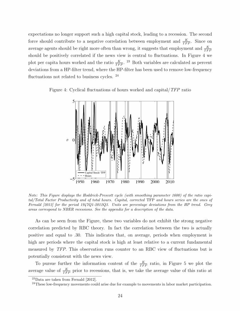
should be positively correlated if the news view is central to fluctuations. In Figure 4 we

plot per capita hours worked and the ratio KTFP

. 23 Both variables are calculated as percent

deviations from a HP-filter trend, where the HP-filter has been used to remove low-frequency

fluctuations not related to business cycles. 24

Figure 4: Cyclical fluctuations of hours worked and capital/TFP ratio

%

1950 1960 1970 1980 1990 2000 2010ï5

0

5

Capital Stock/ TFPHours

Note: This Figure displays the Hoddrick-Prescott cycle (with smoothing parameter 1600) of the ratio capi-tal/Total Factor Productivity and of total hours. Capital, corrected TFP and hours series are the ones ofFernald [2012] for the period 1947Q1-2012Q3. Units are percentage deviations from the HP trend. Greyareas correspond to NBER recessions. See the appendix for a description of the data.

As can be seen from the Figure, these two variables do not exhibit the strong negative

correlation predicted by RBC theory. In fact the correlation between the two is actually

positive and equal to .30. This indicates that, on average, periods when employment is

high are periods where the capital stock is high at least relative to a current fundamental

measured by TFP. This observation runs counter to an RBC view of fluctuations but is

potentially consistent with the news view.

To pursue further the information content of the KTFP

ratio, in Figure 5 we plot the

average value of KTFP

prior to recessions, that is, we take the average value of this ratio at

23Data are taken from Fernald [2012].24These low-frequency movements could arise due for example to movements in labor market participation.

24

the peak of the business cycle and in the three preceeding quarters. According to the news

view of business cycles, recessions should arise after periods where there has been substantial

speculative investment, that is, when KTFP

is high. As can be seen in the figure, almost all

the post war recessions in the US have been preceded by a period where capital accumulation

outstripped growth in TFP. The only exceptions are the recessions of 1973 and 1980. Since

both these recessions are commonly thought as having been driven by energy prices and

monetary factors, not by revised expectations after a period of speculative accumulation, it

is interesting to note that they were not preceded by a period of high capital accumulation.

While most recessions in the sample are preceded by a period of high capital accumulation

relative to the state of technology, the news view of business cycles suggest that high values ofK

TFPshould not be systematically predicting imminent recessions. Instead a high value K

TFP

should often be predicting further expansion. Interestingly, when we examine the correlation

between KTFP

at time t and the growth in hours of employment in the following quarter

(growth between t and t + 1) we find a positive correlation of .24 implying that on average

a high KTFP

ratio predicts further expansion, even though most recessions are preceded by

high values of KTFP

. 25

While the patterns we have reported between the ratio KTFP

and hours worked appear

more consistent with a news view of cycles than an RBC view, it does not yet tell us whether

the observed positive correlation between KTFP

and hours worked results from periods where

capital accumulation is driven mainly by demand– as would be implied by a news view– or

alternatively by supply. In particular, there is an important class of business cycle theories

that suggests that it may be changes in the supply of investment goods that drive the

cycle instead of demand. The mechanism is again technology-related and comes under the

heading of investment-specific technological change. 26 This view of business cycles argues

that surprise improvements in the technology for producing capital goods cause periods

where investment and employment will be high because the price of investment goods is low.

Such a mechanism is consistent with a positive correlation between KTFP

and hours worked.

To differentiate between a story based on the supply of investment goods versus the demand

for investment goods, the first piece of evidence to examine is the behavior of relative prices.

In Table 1 we report the correlation between per capita hours worked and different price

25As a robustness check, we also examined how hours worked co-vary with the ratio of capital to TFPwhen capital is measured in units of consumption goods (as opposed to units of output); that is, when wereplace our previous ratio K

TFP with pKTFP where p is the relative price of investment in terms of consumption

good. For this case, we found very similar cyclical properties and we found again that most recessions (withthe exception of those of the 70s and earlier 80s) were preceded by periods where pK

TFP was high.26See for example Greenwood, Hercowitz, and Huffman [1988], Greenwood, Hercowitz, and Krussell [2000]

and Fisher [2006]

25

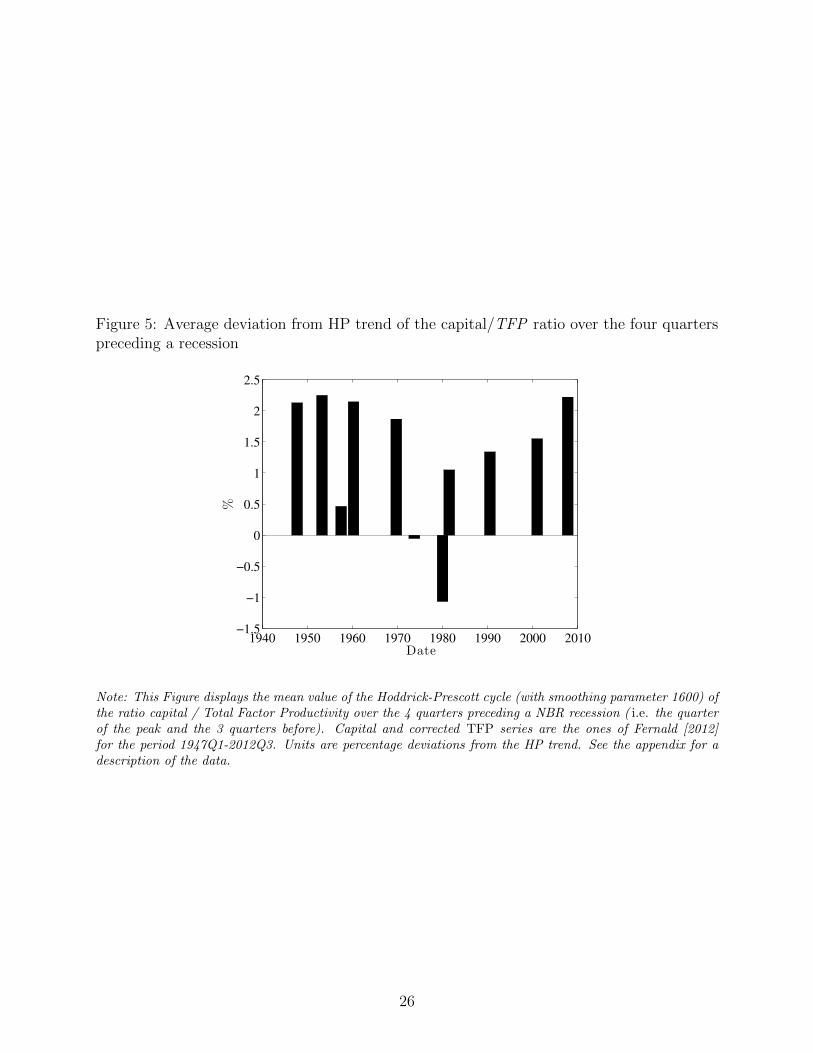
Figure 5: Average deviation from HP trend of the capital/TFP ratio over the four quarterspreceding a recession

1940 1950 1960 1970 1980 1990 2000 2010−1.5

−1

−0.5

0

0.5

1

1.5

2

2.5

Date

%

Note: This Figure displays the mean value of the Hoddrick-Prescott cycle (with smoothing parameter 1600) ofthe ratio capital / Total Factor Productivity over the 4 quarters preceding a NBR recession ( i.e. the quarterof the peak and the 3 quarters before). Capital and corrected TFP series are the ones of Fernald [2012]for the period 1947Q1-2012Q3. Units are percentage deviations from the HP trend. See the appendix for adescription of the data.

26

indexes for capital goods. 27 We report the correlations for two samples, one starting in

1960Q1 and the other one starting in 1987Q4 and corresponding to the post-Volcker period

where nominal prices have been more stable. The investment prices we consider are: the

BEA measures for fixed investment, structures, equipment and residential investment. 28

We also report results using the S&P500 as a measure of the price of investment. This is

closest to the model we have presented where it is the value of having capital goods installed

in firms that is driving fluctuations. All these prices are deflated by the core CPI 29 and

HP-filtered. We see in Table 1 a mixed set of results for the cyclical pattern of the relative

Table 1: Various measures of the relative price of investment, deflating with core CPI,correlations with Hours

Variable 1960Q1-2012Q3 Post-VolckerFixed I 0.42 0.76Struct.I 0.44 0.75Equip.I -0.25 0.17Resid.I 0.70 0.80SP500 0.31 0.56

Note: All variables are quarterly HP filtered with smoothing parameter 1600 and deflated by coreCPI. See the appendix for a description of the data.

price of investment. If we focus on the most recent period where inflation has been stable,

we observe that the relative price of investment is positively correlated with hours worked for

all of our five indexes, with the relation being weak only for the relative price of equipment.

So over this latter period, if investment was driving the cycle then it appears most likely

due to changes in the demand for investment goods as opposed to changes in their supply.

However, if we look at the longer sample, we get a more nuanced picture. The relative price

of fixed investment, structures, residential investment and the stock prices index continue

to show a strong positive relation with employment movements over the longer sample. In

contrast, the relative price of equipment shows a negative co-movement. Hence, over the

longer sample there is room for debate regarding which of investment demand or the supply

of investment goods have more likely played the greater role in fluctuations. From our point

of view, the stock market index is our preferred index since it represents the value to firms

27Throughout this paper, our preferred measure of the cycle is hours worked. We like this measure since itis measured directly and not mechanically related to prices used to construct real output or measured TFP.

28Over the post 1960 period, structures represent 23% of fixed investment, equipment 48% and residentialinvestment 29%.

29We choose to deflate these series by the core CPI to eliminate changes in prices that are due to changesin the price of oil and commodities.

27

of investing to expand their production capacity and the behavior of this index is consistent

with the pattern implied by the news view of fluctuations. Nonetheless we recognize that

different researchers may or may not find the behavior of the relative price of investment

goods, especially the relative price of equipment, to be consistent with the news view.alt

3.2 The non-fundamentalness problem and its implications

Structural vector autoregressive methods have been extensively used to explore the effects

of news shocks on economic aggregates, and we will review this literature in the following

subsection. However, before doing so it is important to note that structural VAR methods

require that the underlying data generating process satisfy certain properties related to the

invertibility of the model’s solution when written in moving average form. In the presence of

news, this property may not hold which can render results from SVAR methods meaningless.

Accordingly, in this subsection our aim is to clarify the extent to which this non-invertibility

problem, or alternatively known as a non-fundamentalness problem, limits the usefulness of

SVAR methods in identifying the effects of news shocks.

3.2.1 Introducing the non-fundamentalness problem using univariate processes

To begin, let us consider a simple economic environment where the solution to the model

generating the data is the one-dimensional stationary 30 stochastic process xt with moving

average (MA) representation given by:

xt = θ0εt + θ1εt−1 + · · ·+ θkεt−k + · · ·

= θ(L)εt.(17)

where εt is a univariate zero mean white noise process with time-invariant variance and un-

correlated components. θ(L) is a polynomial of possibly infinite order, whose coefficients are

absolutely summable. For simplicity, the process xt is assumed to be purely nondeterminis-

tic, with MA roots exactly on the unit circle being excluded. We will refer to this process

as the structural representation of xt , that is, the representation that is derived from a

model where the εt are economically meaningful shocks. The question we want to address

is whether or not an econometrician is able to recover this structural model, i.e. the coeffi-

cients θk and the shock ε from observations of current and past values of xt. The advantage

of first considering a univariate case is that we can focus on the issue of fundamentalness,

30In most of the economic application we will review, variables will be non-stationary. The process x willthen have to be thought as (typically) the first difference of the macroeconomic series under consideration,or as a linear combination of them in the case of a multivariate model with cointegration.

28

without needing to discuss additional issues associated with identification which emerge in

the multivariate multi-shock case.

A shock εt is said to be a fundamental shock (more precisely xt-fundamental 31) if it can

be recovered from observing the current and past observations of x. From the inspection

of (17), it is clear that ε can be expressed as a function of current and past values of x if

and only if the polynomial θ(L) can be inverted, so that εt = [θ(L)]−1xt. The condition

for fundamentalness is therefore that all the roots of θ(L), i.e. the solution to the equation

θ(z) = 0, are strictly outside the unit disc. When the shock in (17) is non-fundamental, the

econometrician will typically not be able to recover the ε shocks from estimating the Wold

representation 32 and therefore will not be able to recover the structural impulse response of

xt to a shock εt.33

We now define a news-rich process as process for which there exists at least one q such

that |θq| > |θ0|. Such processes are of the “news” type in the sense that a larger share of the

variance of xt is attributable to the shock εt−q than to the shock εt, that is, more variance is

due to a shock known q period in advance than due to the current period shock. Structural

models with news shocks, as for example the ones presented in the previous section, generally

have a solution that correspond to a news-rich process.

Our goal in this section is to clarify two points. The first point is qualitative: a model

with news shocks may give rise to a non-fundamental representation but does not necessar-

ily give rise to a non-fundamental representation. The second point is quantitative: when

a model with news shocks gives rise to a non-fundamental representation, its fundamental

representation can be “close” to its non-fundamental representation implying that SVAR

methods may nonetheless deliver a good approximation of structural impulse responses even

when the non-fundamentalness problem arises. 34 To set the stage, we will begin by high-

lighting a negative result, that is, we will show that a model with news shocks may exhibit

a non-fundamentalness problem and this problem can be severe in the sense that its funda-

mental representation will be far from its (structural) non-fundamental representation. The

easiest case to show this problem is in the case where the model’s solution is an MA(1) pro-

cess. However, as we will show, several results from the MA(1) example do not generalize,

and it is for these reasons that the non-fundamentalness issue may not be as serious as it

31See Lutkepohl [2012] for a formal presentation. See also Alessi, Barigozzi, and Capasso [2008] for areview of non-fundamentalness and identification in structural VAR models.

32The Wold representation is the unique linear representation of a stationary process where the shocks arelinear forecast errors.

33Recall that the impulse response function (IRF) of xt to a unit shock εt = 1 is given by the sequence ofMA coefficients θk for k = 0, 1, ....

34To overcome invertibily problems, Lanne and Saikkonen [2011] and [2013] have proposed to directlyestimate non-fundamental representations as non causal autoregressive models.

29

may first appear from the MA(1) example we present below.

Before we proceed, let us notice that if θ0 = 0, then θ(L) = (θ1 + θ2L+ · · · )×L. In this

singular case, z = 0 is a root of θ(z) and the process is non-fundamental. The univariate

processes we are examining in the next section are assumed to be non singular news-rich

processes, with θ0 6= 0, with the normalization θ0 = 1. As the literature has often focussed

on singular news-rich processes, we therefore also examine this case and show that such

singular processes are not qualitatively different if some extra information is given to the

econometrician.

3.2.1.1 The MA(1) case: Consider the following simple rational expectations model:35

xt = aEtxt+1 + yt,

yt = εt + (1 + α)εt−1,

with 0 < a < 1, E(εt) = 0 and E(ε2t ) = σ2. xt is an endogenous variable and yt is the

news-rich exogenous process. The assumption that α > 0 is meant to capture the idea that

εt is a news shock as information obtained today implies expected growth in yt . Solving

this model forward, we obtain

xt =∞∑τ=0

aτEtyt+τ .

Using the process of y, the model’s solution reduces to

xt = (1 + a(1 + α))εt + (1 + α)εt−1.

The solution to the model is therefore a news-rich process if a < α1+α

. Moreover, this is the

same condition that implies non-fundamentalness, as the root of θ(z) will be inside the unit

circle if and only if a < α1+α

. This simple example shows (i) that news shocks (α > 0) do

not necessarily mean non-fundamentalness and (ii) that if the model solution is a news-rich

MA(1), , the εts are not fundamental shocks and therefore cannot be recovered from current

and past observations on xt. In other words, one cannot use the Wold representation of the

data to obtain structurally meaningful impulse responses.

3.2.1.2 Is the fundamental representation close to the non-fundamental repre-

sentation in the MA(1) case? The question we now want to address is, suppose we are

in a situation where the solution to a model is non-fundamental, and the researcher is not

35See Feve, Matheron, and Sahuc [2009] for a similar model but with a singular news-rich process of thetype yt = εt−q with q > 0.

30

aware of the issue and derives an impulse response for xt from its Wold representation. Will

the resulting impulse response be very different from the impulse response for εt implied by

the model?

To explore this, consider the situation where the solution to the model is a news-rich

MA(1) process which in the MA(1) case is equivalent to noting that it is a non-fundamental

process:

xt = εt + (1 + α)εt−1, (18)

with α > 0.

How far from this non-fundamental representation – or structural representation– is the

fundamental representation – or Wold representation? Let the Wold representation be de-

noted by:

xt = εt + θ1εt−1, (19)

where θ1 and σ2 need to be found. We can obtain those two parameters by matching the

autocorrelation functions. Computing variance and autocorrelation from (18) and (19), we

obtain the two equations:E(x2t ) = (1 + (1 + α)2)σ2

ε = (1 + θ21)σ2ε ,

E(xtxt−1) = (1 + α)σ2ε = θ1σ

2ε .

Solving those two equations, we obtain the following fundamental representation

xt = εt +1

1 + αεt−1.

with E(εt) = 0 and E(ε2t ) = (1 + α)2σ2.

As illustrated on Figure 6, the fundamental (Wold) representation gives a impulse re-

sponse function to a unit shock 36 which is very different from the structural one. In partic-

ular, the structural IRF shows a hump shape while the fundamental one is monotonic and

decreasing.

In summary, in the case where the solution of a model with news is a news-rich MA(1) pro-

cess, then the solution is non-fundamental and this non-fundamental solution is qualitatively

different from the fundamental representation. This suggest that the non-fundamentalness

issue is likely very problematic in models with news shocks. However, as the following two

sub-sections will clarify, the MA(1) case may be somewhat misleading because in more gen-

eral settings news-rich processes are not necessarily non-fundamental, and even if they are

non-fundamental, they are not necessarily very different from their fundamental representa-

tion.36All the IRFs are normalized to be the response to a unit shock. Note that if one computes the IRF to

a one standard deviation shock, the fundamental and structural IRF would not start from the same point,as the fundamental and structural shocks have different standard deviations.

31

Figure 6: A structural nonfundamental news-rich MA(1) process and its fundamental rep-resentation

t

xt

0

1

1

1 + α

21

11+α

Structural (non-fundamental)

Fundamental (Wold representation)

Note: This Figure displays the impulse response functions to a unit shock for the structural non-fundamentalprocess (18) and its Wold representation (19).

3.2.1.3 News-rich processes are not necessarily non-fundamental: We now con-

sider the news-rich MA(2) process:

xt = εt + (1 + α)εt−1 + βεt−2, (20)

with α > 0. Can this process be fundamental, or to put it differently can we find conditions

on β under which the two roots of the polynomial θ(z) = βz2 + (1 + α)z + 1 are outside the

unit disc? The answer is yes.

As can be verified, 37 a news-rich MA(2) process is fundamental if and only if α <

β < 1. Panel (a) of Figure 7 displays the IRF of x to a unit structural shock ε in such a

case. Note that contrarily to what the MA(1) case suggests, the process is news-rich and

nevertheless fundamental. Panels (b), (c) and (d) illustrate the three reasons for which non-

fundamentalness could occur: α large, β large given α or β low given α. The invertibility

condition α < β < 1 states that the process need not increase too much between period

0 and period 1 (α < 1) and that it not decline too abruptly between period 1 and period

37The discriminant of the polynomial is ∆ = (1 + α)2 − 4β. If β > (1+α)2

4 , ∆ < 0. Therefore, the tworoots are complex and conjugate. As the product of the root is equal to β−1, the two roots are complex

and outside the unit disc if and only if (1+α)2

4 < β < 1, which defines a non empty set for values of β isα < 1. If ∆ ≥ 0, the two roots of θ are real. Note that θ(0) = 1 > 0, θ(−1) = β − α and θ(1) = 2 + α + β.If 0 < β < α, then θ(−1) < 0. Given that θ(0) = 1 > 0, one root has to be between -1 and 0, and the

structural representation cannot be fundamental. If (1+α)2

4 > β > α, then θ(−1) > 0 and θ(1) > 0 and thetwo real roots of θ(L) have modulus greater than one.

32

2 (β > α)). This example nicely illustrates that news-rich processes may or may not be

fundamental.

Figure 7: News-rich MA(2) processes

(a) Fundamental (b) Nonfundamental: α is too large

t

xt

0

1

1

1 + α

2

2

βα

admissible region for α

admissibleregion for β

3 t

2

0

1

1

1 + α

2

β

3

admissible regionfor α

xt

(c) Nonfundamental: β is too large (d) Nonfundamental: β is too small

t

xt

2

α

0

1

1

1 + α

2

β

3

admissible regionfor α

admissibleregion for β

t

xt

2

α

0

1

1

1 + α

2

β

3

admissible regionfor α

admissibleregion for β

Note: This Figure displays four possible configurations of the MA(2) process (20), by plotting IRF to a unitshock. The MA(2) process is described by the couple (α, β). Condition for fundamentalnes is α < β < 1.

3.2.1.4 Non-fundamental structural news-rich processes can be close to their

fundamental representation: The MA(1) case was very stark in the sense that the

fundamental IRF was qualitatively different from the structural non-fundamental one: the

structural IRF was hump-shaped while the fundamental one was not. We show here that

this is also not a general result. To do so, we again restrict to a MA(2) news-rich processes.

xt = εt + (1 + α)εt−1 + βεt−2,

33

with α > 1 or β 6∈ [α, 1], so that ε is non-fundamental. Let us consider the Wold represen-

tation of this MA(2):

xt = εt + θ1εt−1 + θ2εt−2,

with E(εt) = 0 and E(ε2t ) = σ2. Equating variance, first and second order covariances of the

two representations gives:E(x2t ) = (1 + (1 + α)2 + β2)σ2

ε = (1 + θ21 + θ22)σ2ε ,

E(xtxt−1) = (1 + α)(1 + β)σ2ε = θ1(θ2 + 1)σ2

ε ,E(xtxt−2) = βσ2

ε = θ2σ2ε .

We obtain the three following equations whose unknowns are θ1, θ2 and σ2ε :

σ2ε =

β

θ2σ2ε , (21)

θ1 =(1 + α)(1 + β)

β

θ21 + θ2

, (22)

0 = 1− 1 + (1 + α)2 + β2

βθ2 + θ22 +

((1 + α)(1 + β)

β

)2θ22

(1 + θ2)2. (23)

(23) is an order four equation in θ2 and we know that β is a root of this equation. Knowing

θ2, (21) and (22) trivially gives the values of σ2ε and θ1. Factorizing with (θ2 − β), (23) can

be written as

(θ2 − β)(β2θ32 + β(2β − (1 + (1 + α)2)θ22 + (β2 − 2β + (1 + α)2)θ2 − β

)= 0. (24)

It is hard to find easily interpretable formulas for θ2 and we therefore simply give here a set

of examples. 38 We start with the MA(2) news-rich fundamental process with α = .7 and

.7 < β < 1. We then construct three non-fundamental processes by violating one after the

other the conditions α < 1, β < 1 and β > α. In each case, we move the parameter 20%

above the upper bound of the admissible region for fundamentalness. And for each case,

we compute the Wold representation, which amounts to solving numerically the order three

polynomial (24) and picking up the only real solution for which the θ(L) is invertible.

Results are displayed in Figure 8. As we can see from the figure, in the three cases, the

fundamental IRF to a unit shock is quite close to the structural one. We do not aim at

showing here that in general non-fundamentalness is not quantitatively relevant, but that it

is not true that it is always so 39.

38Mertens and Ravn [2010] and Offick and Wohltmann [2013] discuss of a case in which analytical resultscan be obtained. If xt = aEtxt+1 + εt−q with |a|< 1, then the model solution is xt = Θq(L)εt, withΘq(L) =

∑qi=0 q

q−iLi. Such a lag polynomial is closely related to a cyclotomic polynomial, so that its roots

34

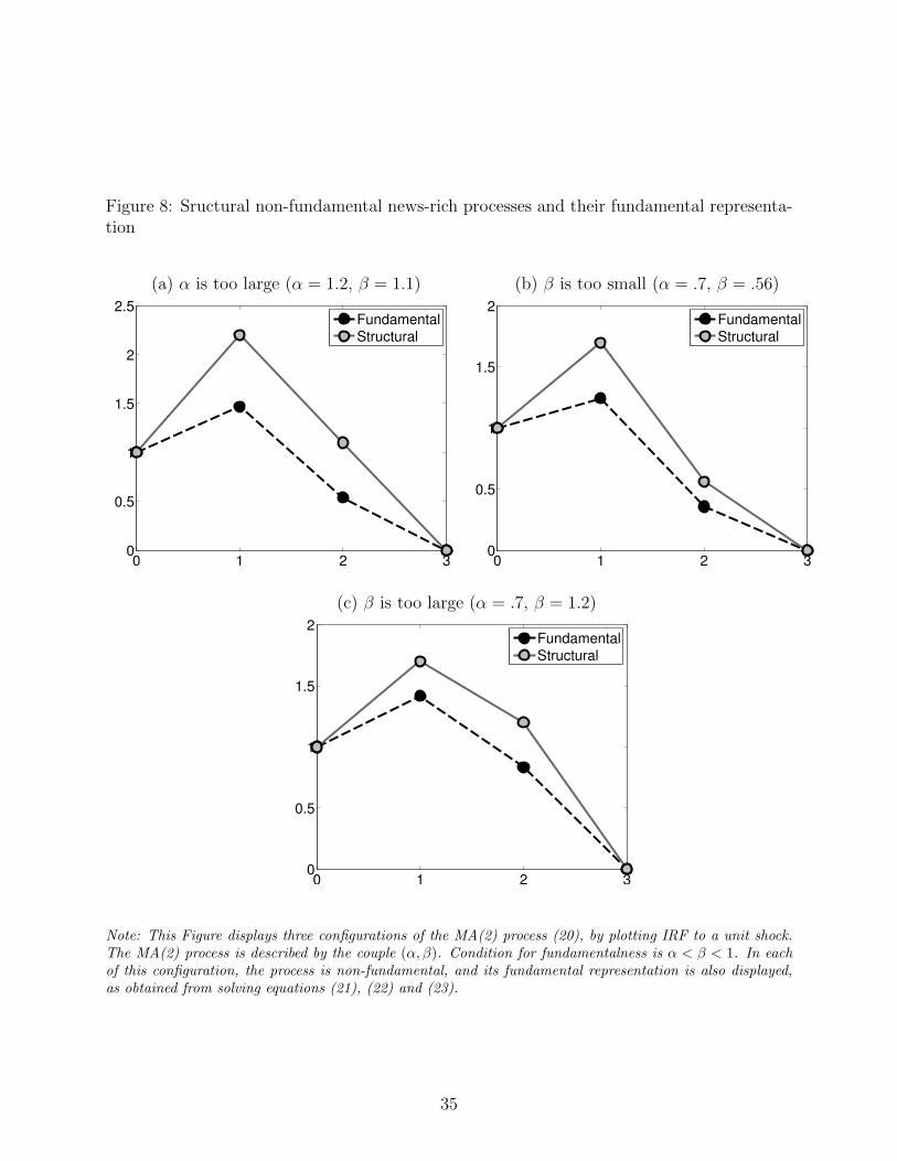
Figure 8: Sructural non-fundamental news-rich processes and their fundamental representa-tion

(a) α is too large (α = 1.2, β = 1.1) (b) β is too small (α = .7, β = .56)

0 1 2 30

0.5

1

1.5

2

2.5

Fundamental

Structural

0 1 2 30

0.5

1

1.5

2

Fundamental

Structural

(c) β is too large (α = .7, β = 1.2)

0 1 2 30

0.5

1

1.5

2

Fundamental

Structural

Note: This Figure displays three configurations of the MA(2) process (20), by plotting IRF to a unit shock.The MA(2) process is described by the couple (α, β). Condition for fundamentalness is α < β < 1. In eachof this configuration, the process is non-fundamental, and its fundamental representation is also displayed,as obtained from solving equations (21), (22) and (23).

35

3.2.1.5 The role of information: The previous MA(2) examples have illustrated that

non-fundamentalness does not necessarily render Wold representations useless for under-

standing the effects of structural shocks. Instead, it suggests that the problem is quantitative

in nature, and depends on the quantity of information in the current and past realizations of

the observable variables. In the next section, we will analyze multivariate processes and show

that the quantity of information available to the econometrician matters for invertibility and

for the distance between the structural representation and the fundamental one. As a pre-

lude to the more general result, intuition about the relation between the information set and

non-fundamentalness can be obtained in the following simple case where we again consider

the MA(1) news-rich process, but now also allow for singularity, as θ0 is not restricted to be

non zero:

xt = θ0εt + (θ0 + α)εt−1,

with (for simplicity) θ0 ≥ 0 and α > 0. We know from the previous analysis that ε in

this case is non-fundamental, more precisely xt-non-fundamental if we only have information

on xt. Let us now enlarge the observation set of the econometrician by allowing for the

observation of a second variable yt that contains information about εt (typically, on would

think of an asset price variable in the case of technological news shocks). In order to avoid

non-generic singularities, we assume that there is a second shock νt (with Eνt = 0) that we

interpret as pure noise. To save notations, let’s normalize the covariance matrix of (ε, ν) to

the identity matrix. The structural model is therefore given by

xt = θ0εt + (θ0 + α)εt−1 + νt, (25)

yt = γεt + νt, (26)

with γ > 0 for simplicity. Its matrix representation is(xtyt

)=

(θ0 + (θ0 + α)L) 1γ 1

)(εtνt

)= Θ(L)

(εtνt

).

The process will be invertible, and therefore ε will be fundamental, when the roots of the

determinant of the matrix Θ(z) are outside the unit disk. In this case, the determinant of

Θ(z) has only one root which is z = γ−θ0θ0+α

.

If γ = 0, meaning that y is uninformative about ε, then |z| < 1 and ε is non-fundamental,

which is the result we had in the previous section. But if y is informative enough about ε,

can be computed analytically.39Lippi and Reichlin [1993] show that the structural shocks estimated by Blanchard and Quah [1989] can be

non fundamental in a model in which productivity follows an exogenous news-rich process. Such a diffusionprocess is also analyzed in Lippi and Reichlin [1994b]. Lippi and Reichlin [1994a] show that nonfundamentalrepresentations can be obtained by the use of Blaschke matrices. Blanchard and Quah [1993] underline thefact that structural representations can be non fundamental but close to the fundamental one.

36

meaning that γ is large enough (precisely γ > 2θ0 + α), then ε is fundamental. In the

case where γ < 2 + α, then ε is not fundamental, but it will be “close” to the fundamental

shock if γ is high enough, or in other words if y is informative enough about ε. Note that

there is now nothing specific with singular news-rich processes. When θ0 = 0, the condition

for invertibility writes γ > α: that is, the signal needs to be informative enough to allow

invertibility. We now formally discuss the role of information in a general multivariate case.

3.2.2 The multivariate case

Consider an economic model who has a representation for yt in the state-space form

xt+1 = Axt +Bεt, (27)

yt = Cxt−1 +Dεt. (28)

xt is n × 1 vector of possibly unobserved state variables, yt is a k × 1 vector of variables

observed by the econometrician, and εt is m × 1 vector of structural shocks. The shocks ε

are Gaussian vector white noise with Eεt = 0, Eεtε′t = I and Eεtεt−j = 0 for j 6= 0. We

restrict to the “square case” in which there are as many shocks as observables in y (k = m)

and in which D has full rank. Our discussion in this section closely follows the presentation

of Fernandez-Villaverde, Rubio-Ramırez, Sargent, and Watson [2007] and Sims [2012].

The question we ask is whether or not one can recover the structural shocks from the

following VAR that involves only the observable variables y:

yt = F (L)yt−1 +Gεt, (29)

where F (L) is a infinite order lag polynomial. In other words, does there exist an F (L) and

a matrix G such that εt = εt?

Note that the answer to the question relies on two different sets of properties. First,

assuming perfect observability of the state variables (y = x), the question is whether the

VAR process (27) is invertible, which is a constraint on A. Second, given that information is

imperfect, is the informational content of y enough to recover the structural shocks, which

is a constraint on C and D given A and B. Fernandez-Villaverde, Rubio-Ramırez, Sargent,

and Watson [2007] derive what they call a poor man’s invertibility condition. If the matrix

A − BD−1C is stable (meaning that all its eigenvalues are inside the unit disc), then the

structural shocks εt are the innovations of VAR (29), meaning that there are the fundamental

ones. Let us follow Sims [2012] to show this. Solve for εt in (28):

εt = D−1(yt − Cxt−1),

37

then plug into (27):

xt = (A−BD−1C)xt−1 +BD−1yt.

Solving backward yields

xt = (A−BD−1C)t−1x0 +t−1∑τ=0

(A−BD−1C)τ−1BD−1yt−τ . (30)

If limt→∞(A− BD−1C)t−1 = 0 (which is the case if (A− BD−1C) is a stable matrix), then

the history of observables perfectly reveals the current state. One can then plug (30) in (28)

to obtain a VAR in obervables whose innovations are ε:

yt = Ct−1∑τ=0

(A−BD−1C)τ−1BD−1yt−1−τ +Dεt.

The structural shocks ε are therefore fundamental. Note that one will still need to make

identifying assumption related to D to recover the ε from the VAR innovations, which is a

key issue in Structural VAR methods discussed in the next section.

If A − BD−1C is not stable, then the structural shocks cannot be obtained from the

estimation of a VAR like (29). In such a case, how close will be the fundamental shocks

to the structural one depends on how much information is contained in y. As shown in

Sims [2012], one can use the Kalman filter to form a forecast of the current state, x, given

observables and a lagged forecast:

xt = (A−KC)xt−1 +Kyt, (31)

where K is the time invariant Kalman gain and A − KC a stable matrix under some sta-

bilizability and detectability conditions (see Hansen and Sargent [2012], chapter 8). Let us

denote by xt = xt− xt the forecast error of the filter and Σ its variance matrix. Adding and

substracting Cxt from (28), on obtains

yt = Cxt−1 + ut, (32)

with

ut = C(xt−1 − xt−1) +Dεt. (33)

Using lagged (31), substituting in (32) and solving backward gives, when t→∞ and using

the fact that (A−KC) is a stable matrix:

yt = Ct−1∑τ=0

(A−KC)τKyt−1−τ + ut. (34)

38

This VAR representation in observables have innovations u which are linear combination of

the structural shocks ε and errors in forecasting the states x. The innovations variance is

given by

Σu = CΣC ′ +DD′,

where we use the assumption that ε has an identity variance matrix.

When the poor man’s invertibility condition holds, Fernandez-Villaverde, Rubio-Ramırez,

Sargent, and Watson [2005] 40 show that Σ = 0, so that the structural shock is fundamental.

When that condition does not hold, Σ 6= 0, and the innovation variance from the VAR

is strictly larger than the innovation variance in the structural model. Invertibility fails

because the observables do not allow for full revelation of the state vector. Put that way, it

becomes clear that non-invertibility is fundamentally an issue of missing information 41. As

Sims [2012] puts it clearly, non-invertibility is not an “either/or” problem, as we have already

illustrated in the univariate MA(2) case. If Σ is non zero but small (meaning that its spectral

radius is close to zero), then ut is almost equal to Dεt. This implies that SVAR methods

may provide good approximations to the effects of structural shocks even in the presence of

non-fundamentalness. Sims [2012] and Seymen [2012] provide Monte Carlo evidence showing

this to be the case in a reasonably calibrated macroeconomic model with news shocks. 42

Feve and Jidoud [2012a] also consider a stylized dynamic model with news shocks in which

the model solution is an infinite order non fundamental VAR. They show that even in such

a case, finite order non fundamental VARs approximated quite well the model solution. 43

40Fernandez-Villaverde, Rubio-Ramırez, Sargent, and Watson [2005] NBER working paper is an extendedversion of Fernandez-Villaverde, Rubio-Ramırez, Sargent, and Watson [2007]

41This interpretation of the econometrician being “short of observations on a sufficient number of series”is the one of Hansen and Sargent [1994]. It suggests a way to test for non-fundamentalness, as formalizedby Forni and Gambetti [2011]. They characterize necessary and sufficient conditions under which a setof variables is informationally sufficient in a VAR, i.e. that it contains enough information to estimatethe structural shocks. Then, they propose a testing procedure based on such conditions, which relies onthe fact that the estimated “structural” shocks of the VAR should not be Granger-caused by the principalcomponents of a large Factor Augmented VAR.

42Fernandez-Villaverde and Rubio-Ramırez [2006] evaluate nonfundamentalness in a DSGE linearized solu-tion. They consider the monetary model of Christiano, Motto, and Rostagno [2003] and study two 8-variableVARs with two different sets of observables from the model. They show that one of the two is fundamentalwhile the other one is not. This nicely illustrate that fundamentalness is essentially a question of informationsets. Forni, Giannone, Lippi, and Reichlin [2009] have developed Factor Augmented VARs that use a largenumber of variables (hundreds) in order to avoid nonfundamentalness.

43See Feve and Jidoud [2012b] for a discussion of short run and long run identification in such an analyticalcase.

39

3.3 Structural VAR evidence

In this section we will discuss how SVAR methods have been used to evaluate the relevance

and effects of news shocks. As emphasized in the previous section, the appropriateness of

using VARs to discuss structural shocks relies on the structural shocks either being funda-

mental or that the non-fundamentalness problem –if present– is not quantitatively severe.

We will assume this to be the case in this section, recognizing that the caveats discussed in

the previous section may raise doubts about this assumption.

The earliest work using VARs and discussing results in terms of news is Cochrane [1994]

using a bi-variate consumption and income VAR. It followed a couple of papers by Blanchard

and Hall. Looking for the sources of the 1990-91 US recession, Blanchard [1993] and Hall

[1993] concluded that the recession was likely to have been caused by a shock to consumption.

As Cochrane [1994] put it, “since consumption is an endogenous variable, the ultimate source

of variability must be news about future values of any the above”, the “above” variables

being “factor prices, especially oil, monetary policy, government purchases, tax increases,

technology shocks, bank regulation, international factors, and sectoral shifts”.

Beaudry and Portier [2006] focused this idea by examining the potential effects of news

regarding technological opportunities. Since much of the SVAR literature on news pursued

this narrower interpretation, we will begin by presenting the approach used Beaudry and

Portier [2006] and we will implement it on a more up-to-date sample. We then extend the

analysis to higher dimension VARs and present different routes the literature has taken to

identify technological news shocks.

The central idea in Beaudry and Portier [2006] is that financial variables, and especially

stock prices, are the type of variables most likely to reflect news as they are clearly forward

looking and free to jump in response to revised expectations. Hence, to look at the relevance

of technological news, one can look at the extent to which innovations in stock prices con-

tain information about future technological growth, or alternatively whether periods of high

technological growth are preceeded by increase in stock prices. Beaudry and Portier [2006]

implemented this idea using alternatively a short run and a long run identification scheme

in a bi-variate setting.

3.3.1 A bivariate SVAR

Let us start from a situation where we already have an estimated Wold representation for

the bivariate system composed of Total Factor Productivity (TFPt) and a stock prices index

(SPt). This moving average representation is given by (for ease of presentation we neglect

40

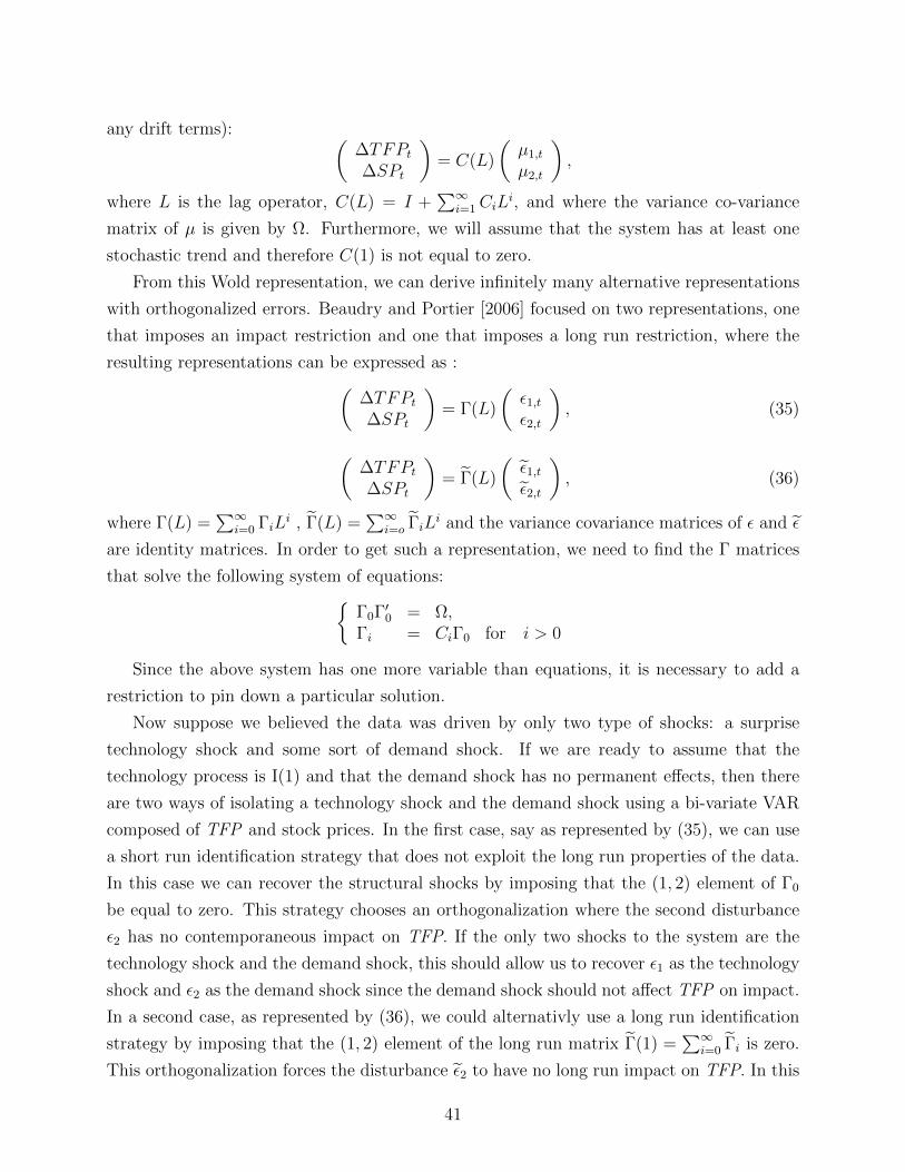
any drift terms): (∆TFPt∆SPt

)= C(L)

(µ1,t

µ2,t

),

where L is the lag operator, C(L) = I +∑∞

i=1CiLi, and where the variance co-variance

matrix of µ is given by Ω. Furthermore, we will assume that the system has at least one

stochastic trend and therefore C(1) is not equal to zero.

From this Wold representation, we can derive infinitely many alternative representations

with orthogonalized errors. Beaudry and Portier [2006] focused on two representations, one

that imposes an impact restriction and one that imposes a long run restriction, where the

resulting representations can be expressed as :(∆TFPt∆SPt

)= Γ(L)

(ε1,tε2,t

), (35)

(∆TFPt∆SPt

)= Γ(L)

(ε1,tε2,t

), (36)

where Γ(L) =∑∞

i=0 ΓiLi , Γ(L) =

∑∞i=o ΓiL

i and the variance covariance matrices of ε and ε

are identity matrices. In order to get such a representation, we need to find the Γ matrices

that solve the following system of equations:Γ0Γ

′0 = Ω,

Γi = CiΓ0 for i > 0

Since the above system has one more variable than equations, it is necessary to add a

restriction to pin down a particular solution.

Now suppose we believed the data was driven by only two type of shocks: a surprise

technology shock and some sort of demand shock. If we are ready to assume that the

technology process is I(1) and that the demand shock has no permanent effects, then there

are two ways of isolating a technology shock and the demand shock using a bi-variate VAR

composed of TFP and stock prices. In the first case, say as represented by (35), we can use

a short run identification strategy that does not exploit the long run properties of the data.

In this case we can recover the structural shocks by imposing that the (1, 2) element of Γ0

be equal to zero. This strategy chooses an orthogonalization where the second disturbance

ε2 has no contemporaneous impact on TFP. If the only two shocks to the system are the

technology shock and the demand shock, this should allow us to recover ε1 as the technology

shock and ε2 as the demand shock since the demand shock should not affect TFP on impact.

In a second case, as represented by (36), we could alternativly use a long run identification

strategy by imposing that the (1, 2) element of the long run matrix Γ(1) =∑∞

i=0 Γi is zero.

This orthogonalization forces the disturbance ε2 to have no long run impact on TFP. In this

41

case, ε1 should represent the technology shock and ε2 should represent the demand shock

as only the technology should have a long run effect on measured TFP. If we perform both

these exercise, we can then look at the correlation between the shocks derived from the two

different identification strategies. For example, suppose we look at the correlation between

ε2 and ε1. If the data is driven by only a surprise technology shock and a demand shock,

then the correlation between these two shocks should be zero as one represents the demand

disturbance and the other the supply disturbance. This is the exercise performed in Beaudry

and Portier [2006]. 44

We replicate the estimation of Beaudry and Portier [2006] here, where we extend the

sample to cover the period from 1947Q1 to 2012Q3 as opposed to the period 1947Q1-2000Q1

in the original paper. All the VARs will be estimated with 3 lags in the VECM form, and

4 pages when estimation is done in levels. Panels (a) and (b) of Figure 9 present impulse

responses to a ε2 shock identified using the short run identification strategy discussed above.

The results obtained closely replicate the patterns reported in Beaudry and Portier [2006]

even if the sample is extended. 45 The first observation is that the innovation to the stock

market, ε2, that is orthogonal to current TFP by construction, does not affect TFP for about

10 quarters, but does permanently affect TFP in the long run (panel (a)). This shock is

by design reflected instantaneously in the stock market (panel (b)), but interestingly stock

prices respond once and for all to this disturbance with little short run dynamics. In panels

(c) and (d) of Figure 9 we report impulse responses associated with the ε1 shock identified

using the long run identifying restriction. Under the assumption that the data are driven by

a surprise technology shock and a demand shock, the responses reported in panels (c) and (d)

should be quite different to those obtained in panels (a) and (b) since one should represent

the effects of a demand shock while the other should represent the effects of a supply shock.

Instead we see by comparing the panels that the responses of each variable are strikingly

similar. This similarity is further illustrated on Figure 10 where we plot ε1 against ε2. While

one could have expected these shocks to be almost orthogonal, the two shocks are instead

44Haertel and Lucke [2008] apply the same procedure on German data with similar results. Beaudryand Portier [2005] and Vukotic [2011] perform the same type of identification of news shocks using sectoraldata. Lanne and Luetkepohl [2008] use the same bivariate system but estimate a two-state Markov regimeswitching model. Imposing orthogonality of the two socks in each of the two regimes allows for identificationof two shocks, so that short and long run identification restrictions can be tested.

45Because of space limitations, we do not present robustness results for alternative specification of thisVAR. The punchline is that the properties of these two identification schemes imposed on a bi-variate VARwith U.S.TFP and stock prices is a very robust result with respect to lag length and to estimating the VARin level or as a VECM. However, if one starts from estimating a VAR in differences with non-co-integrationimposed the results change quite substantially as we will show later. Also, the properties depend on using ameasure of TFP that corrects for capacity utilization. If one uses a measure of TFP that does not correctfor capacity utilization, then the response of TFP to a news shock (as associated with either ε2 or ε1) ismuch quicker.

42

closely aligned on the 45 degree line, meaning that they are almost indistinguishable one

from another.

While the patterns in Figure 9 do put into question a two-shock model of the economy

driven by a surprise technology shock and a demand shock, the relevant question is whether

the patterns reported in the panels tell us anything regarding news or other models of

the economy. In Beaudry and Portier [2006] it is argued that one simple interpretation

of these observations is that they are driven by a two shock model where one shock is a

technological news shock and the other a surprise trend-stationary technology shock. Under

this interpretation, the shock ε2 should capture the news shock as it should be reflected

in stock prices before it is reflected in TFP. If in addition we assume that news relates to

permanent changes to TFP, then ε1 identified using the long run restrictions should also

isolate the news shock, thereby explaining the similarity in responses. In that sense, ε2 and

equivalently ε1 correspond to two ways of isolating news about further productivity that

are instantaneously priced in the stock market, although the news does not lead to actual

increases in productivity for a rather long time. As noted, the results from this SVAR

exercise place doubt on the common interpretation of the economy driven primarily by a

demand shock and a surprise technology shock since, if this were the case, innovations in

stock prices which are orthogonal to TFP should reflect the demand shock and should not

resemble supply shocks identified by long run restrictions. 46

3.3.2 Extending to a higher dimension VARs

3.3.2.1 Three-variable VARs: There are at least three reasons for exploring the ro-

bustness of the Beaudry and Portier’s [2006] findings to higher dimension VARs. 47 First,

as we have discussed before, increasing the information set reduces the likelihood of non-

fundamentalness problems. Second, if this identification scheme is identifying the effects of

news, it is interesting to know how other variables respond to news, and this can be explored

by considering a larger VAR. Third, there are likely more than two types of shocks that drive

macro-fluctuations and therefore considering a system with more shocks appears desirable.

However, the drawback or difficulty with a larger system is that it requires more identifica-

46It is important to recognize that this “news” interpretation is not the only possible interpretation ofthese observations. For example, an alternative view is that TFP is endogenous, and that short run nontechnological intrinsic shocks (preference, government spending, taxes, etc...) eventually affect TFP. Such aview would be for example supported by an endogenous growth model with learning by doing.

47Beaudry and Portier [2006] do not only focus on a bi-variate VAR. They also report results for largersystems. However, as noted by Kurmann and Mertens [2013] and formally shown in Lucke [2010], some ofthe identification schemes used for larger systems in Beaudry and Portier [2006] may be problematic (in thecase of long run restrictions and when the system is not estimated in levels). For this reason, we do notreport results from such schemes here, and instead provide new results.

43

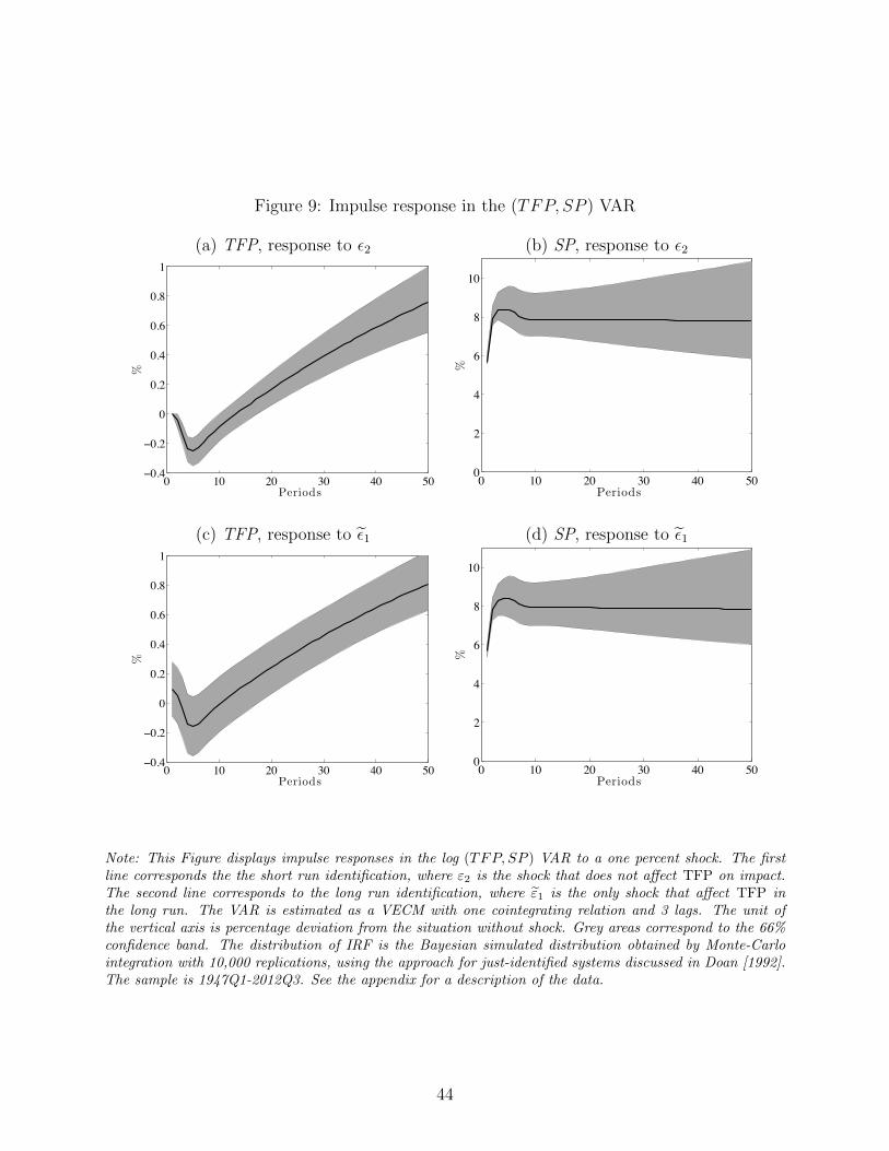
Figure 9: Impulse response in the (TFP, SP ) VAR

(a) TFP, response to ε2 (b) SP, response to ε2

0 10 20 30 40 50ï0.4

ï0.2

0

0.2

0.4

0.6

0.8

1

Periods

%

0 10 20 30 40 500

2

4

6

8

10

Periods

%

(c) TFP, response to ε1 (d) SP, response to ε1

0 10 20 30 40 50ï0.4

ï0.2

0

0.2

0.4

0.6

0.8

1

Periods

%

0 10 20 30 40 500

2

4

6

8

10

Periods

%

Note: This Figure displays impulse responses in the log (TFP, SP ) VAR to a one percent shock. The firstline corresponds the the short run identification, where ε2 is the shock that does not affect TFP on impact.The second line corresponds to the long run identification, where ε1 is the only shock that affect TFP inthe long run. The VAR is estimated as a VECM with one cointegrating relation and 3 lags. The unit ofthe vertical axis is percentage deviation from the situation without shock. Grey areas correspond to the 66%confidence band. The distribution of IRF is the Bayesian simulated distribution obtained by Monte-Carlointegration with 10,000 replications, using the approach for just-identified systems discussed in Doan [1992].The sample is 1947Q1-2012Q3. See the appendix for a description of the data.

44

Figure 10: Short run residuals ε2 against long run ones ε1 in the (TFP, SP ) VAR

ï4 ï3 ï2 ï1 0 1 2 3

ï4

ï3

ï2

ï1

0

1

2

3

SR residuals ε2

LR

residuals

ε1

Note: This Figure displays short run residuals ε2 against long run ones ε1 in the log (TFP, SP ) VAR. ε2 isthe shock that does not affect TFP on impact in the short run identification. ε1 is the only shock that affectTFP in the long run in the long run identification. The VAR is estimated as a VECM with one cointegratingrelation and 3 lags. The sample is 1947Q1-2012Q3. See the appendix for a description of the data.

45

tion assumptions. We will review several different identifying assumptions that have been

made in the literature. To begin, we will focus on the following simple approach to identify-

ing news shocks. To see how the approach can be applied to systems with many variables,

consider a vector of macroeconomic times series of dimension n, whose Wold representation

is estimated to be (again neglecting drift terms):∆X1t

∆X2t...

∆Xnt

= C(L)

µ1,t

µ2,t...µnt

. (37)

Where the two first variables in the system are always TFP and stock prices, X1t = TFPt and

X2t = SPt, while the n− 2 other variables can be different from one system to another. We

aim at identifying some of the structural shocks from the following alternative representation

with orthogonal innovations: ∆X1t

∆X2t...

∆Xnt

= Γ(L)

ε1,tε2,t...εnt

. (38)

To fully identify the n structural innovations, we need n(n−1)/2 restrictions. As we aim

at identifying news shocks about future productivity, we can consider a subset of restrictions

that will allow us to identify only the news shock and a surprise technology shock. To do

this, we first assume that only two shocks can permanently affect TFP in the long run.

This amounts to imposing n− 2 zeros for the last n− 2 columns of the first line of the long

run matrix Γ(1). We then need to separate those two technology shocks: this is done by

assuming that the surprise technology shock is the only shock that affects TFP on impact,

which implies that the only non-zero term in the first row of the impact matrix Γ0 is the

(1, 1) term. These 2n− 3 restrictions allows for a unique identification of the news shock ε2

and the surprise technology shock ε1.

Figure 11 displays the responses of TFP and stock prices to the ε2 shock (the expected

news shock) estimated using a tri-variate system where the third variable is varied. Con-

fidence bands are the ones obtained for the (TFP, SP,C) system, and the four bold lines

correspond to the response in the four three-variable VARs in which the third variable is

alternatively C, I, Y and H (ie, per capita values of consumption, investment, output and

hours worked). All estimations are in levels. Two main conclusions can be drawn from theses

responses: firstly the responses stay the same when we change the third variable in the sys-

tem; secondly, the responses are remarkably similar to the ones obtained in the two-variable

case.

46

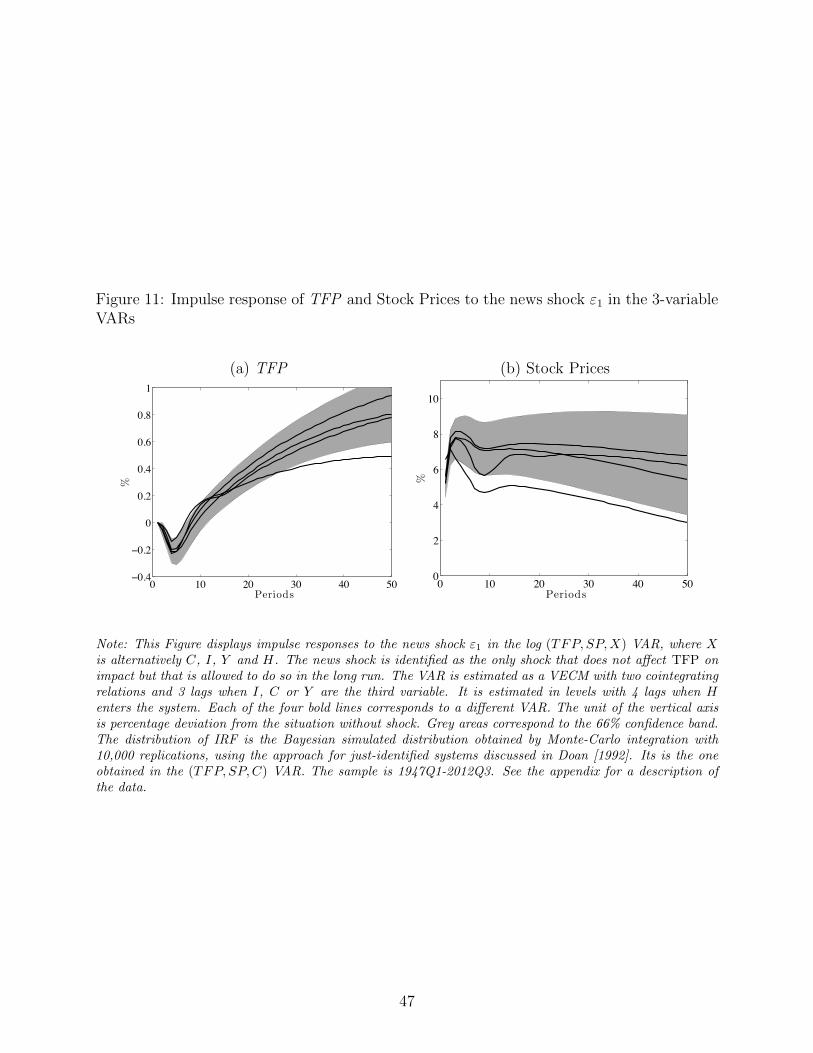
Figure 11: Impulse response of TFP and Stock Prices to the news shock ε1 in the 3-variableVARs

(a) TFP (b) Stock Prices

0 10 20 30 40 50ï0.4

ï0.2

0

0.2

0.4

0.6

0.8

1

Periods

%

0 10 20 30 40 500

2

4

6

8

10

Periods

%

Note: This Figure displays impulse responses to the news shock ε1 in the log (TFP, SP,X) VAR, where Xis alternatively C, I, Y and H. The news shock is identified as the only shock that does not affect TFP onimpact but that is allowed to do so in the long run. The VAR is estimated as a VECM with two cointegratingrelations and 3 lags when I, C or Y are the third variable. It is estimated in levels with 4 lags when Henters the system. Each of the four bold lines corresponds to a different VAR. The unit of the vertical axisis percentage deviation from the situation without shock. Grey areas correspond to the 66% confidence band.The distribution of IRF is the Bayesian simulated distribution obtained by Monte-Carlo integration with10,000 replications, using the approach for just-identified systems discussed in Doan [1992]. Its is the oneobtained in the (TFP, SP,C) VAR. The sample is 1947Q1-2012Q3. See the appendix for a description ofthe data.

47

Figure 12 shows how four macroeconomic aggregates react to the news shock: consump-

tion, investment, GDP and hours worked all increase on impact. Consumption’s response

is close to a once for all jump, while investment, hours and GDP display a hump shape

response in the short run. As shown in Table 2, the news shock explains between 60 and

80 % of the variance of C, I, Y and H for horizons between 4 and 16 quarters, although it

explains less that 3% of the variance of TFP at the same horizon, and about one half of its

variance in the long run. Note from the Table that the short run variance decomposition is

robust to level or VECM specification. We also see in Table 2 that long run properties are

not invariant to the co-integration rank specification : the news shock explains more than

80% of the variance of TFP in the VECM specification, 48 but only one half in the level

one. 49 The possible sensitivity of results to co-integration assumptions will be a recurring

theme. Let us nevertheless stress that although co-integration assumptions do matter for

the long run, they do not affect much the short run dynamics in response to a news shock

as long as the model is not estimated in first-difference i.e. with 0 co-integrating relation.

To illustrate this point, we have estimated a 4-variable VAR with (TFP, SP,C, I) with 0

to 4 co-integrating relations and used our identification to separate news and technological

surprises. Impulse responses of TFP and SP to a news shock are displayed on Figure 13.

The dashed line corresponds to the 0 co-integration case. Note that as long as some long run

information about the relation between TFP and SP is kept, results are very similar. But

when the VAR is estimated in first-difference, this long run relation is lost, and the VAR

estimates a quite counter-intuitive negative long run relation between TFP and SP levels.

3.3.2.2 Consumer confidence: In the above VAR exercises, we have been using infor-

mation from stock prices to help identify news shocks. It is reasonable to believe that stock

prices are good indicators of agents’ perceptions about future economic outcomes. However,

it is interesting to ask whether the news shocks identified using the combination of short and

long run restrictions suggested in this subsection are also reflected in measures of consumer

confidence. If it were not the case, this would put in to question the interpretations of these

shocks. 50 To this end, we examined how measured consumer confidence – as captured

48The results from the VECM system are likely more credible as results from estimating the system inlevels may not lead to consistent estimates of forecast variances. See Phillips [1998] on that point.

49The proper co-integration rank is questionable when hours enter the system, as there is an open debateon the proper specification of hours (level or difference) (see Christiano, Eichenbaum, and Vigfusson [2004],Chari, Kehoe, and McGrattan [2008] and Feve and Guay [2010]). We have verified that this issue is notvery important in this system as the response of hours is very similar when the VAR is estimated with oneco-integrating relation involving only TFP and SP and hours in levels or in difference.

50Sill [2009], Leduc and Sill [2010] and Barsky and Sims [2012] explore the relationship between economicactivity measures of consumer confidence. Lamla, Lein, and Sturm [2007] identify news shocks makinguse of the business tendency surveys of the German Ifo Institute. Milani and Rajbhandari [2012b] exploit

48

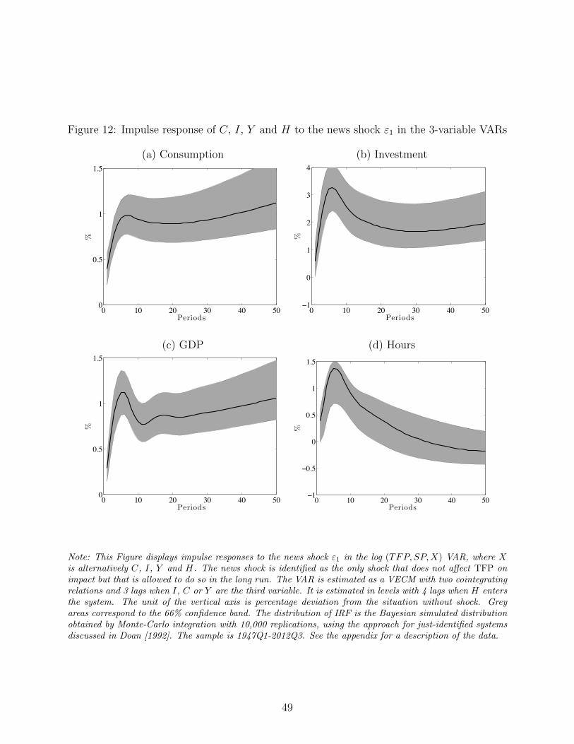
Figure 12: Impulse response of C, I, Y and H to the news shock ε1 in the 3-variable VARs

(a) Consumption (b) Investment

0 10 20 30 40 500

0.5

1

1.5

Periods

%

0 10 20 30 40 50ï1

0

1

2

3

4

Periods

%

(c) GDP (d) Hours

0 10 20 30 40 500

0.5

1

1.5

Periods

%

0 10 20 30 40 50ï1

ï0.5

0

0.5

1

1.5

Periods

%

Note: This Figure displays impulse responses to the news shock ε1 in the log (TFP, SP,X) VAR, where Xis alternatively C, I, Y and H. The news shock is identified as the only shock that does not affect TFP onimpact but that is allowed to do so in the long run. The VAR is estimated as a VECM with two cointegratingrelations and 3 lags when I, C or Y are the third variable. It is estimated in levels with 4 lags when H entersthe system. The unit of the vertical axis is percentage deviation from the situation without shock. Greyareas correspond to the 66% confidence band. The distribution of IRF is the Bayesian simulated distributionobtained by Monte-Carlo integration with 10,000 replications, using the approach for just-identified systemsdiscussed in Doan [1992]. The sample is 1947Q1-2012Q3. See the appendix for a description of the data.

49

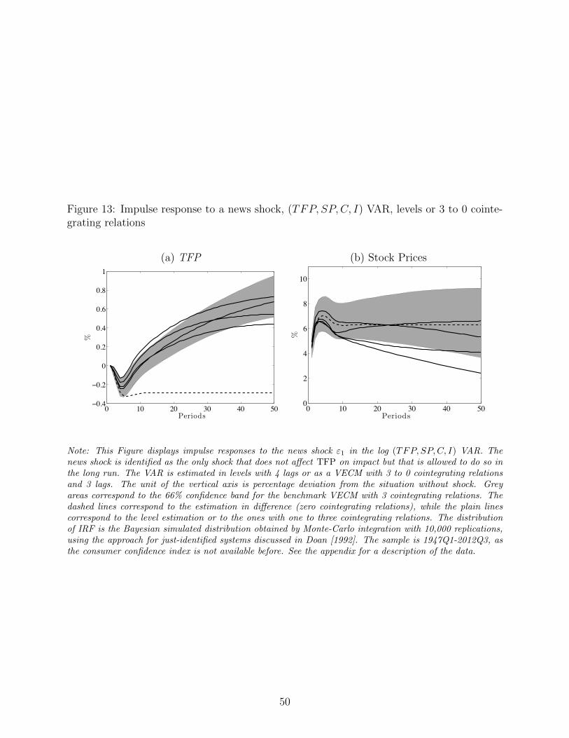
Figure 13: Impulse response to a news shock, (TFP, SP,C, I) VAR, levels or 3 to 0 cointe-grating relations

(a) TFP (b) Stock Prices

0 10 20 30 40 50ï0.4

ï0.2

0

0.2

0.4

0.6

0.8

1

Periods

%

0 10 20 30 40 500

2

4

6

8

10

Periods

%

Note: This Figure displays impulse responses to the news shock ε1 in the log (TFP, SP,C, I) VAR. Thenews shock is identified as the only shock that does not affect TFP on impact but that is allowed to do so inthe long run. The VAR is estimated in levels with 4 lags or as a VECM with 3 to 0 cointegrating relationsand 3 lags. The unit of the vertical axis is percentage deviation from the situation without shock. Greyareas correspond to the 66% confidence band for the benchmark VECM with 3 cointegrating relations. Thedashed lines correspond to the estimation in difference (zero cointegrating relations), while the plain linescorrespond to the level estimation or to the ones with one to three cointegrating relations. The distributionof IRF is the Bayesian simulated distribution obtained by Monte-Carlo integration with 10,000 replications,using the approach for just-identified systems discussed in Doan [1992]. The sample is 1947Q1-2012Q3, asthe consumer confidence index is not available before. See the appendix for a description of the data.

50

Table 2: Share of the variance explained by the news shock in 3-variable VARs (in %)

Horizon 1 4 8 12 16 120Level specification

TFP 0 2 2 2 3 56C 39 71 77 77 75 67I 16 53 65 66 65 57Y 30 72 82 80 78 64H 39 70 81 82 79 56

2 coint. relations specificationTFP 0 2 2 2 4 84C 22 55 63 65 66 87I 5 36 50 52 53 78Y 4 49 64 64 65 87

Note: This table is obtained from the estimation of a (TFP, SP,X) VAR, where X is alternatively C, I,Y and H. The news shock is identified as the only shock that does not affect TFP on impact but that isallowed to do so in the long run. The VAR is estimated as a VECM with two cointegrating relations and 3lags when I, C or Y are the third variable. It is estimated in levels with 4 lags when H enters the system.Results for TFP are given for the TFP, SP,C) VAR. The sample is 1947Q1-2012Q3. See the appendix fora description of the data.

by the Michigan survey – reacts to a news shock in a 3-variable VAR where the first two

variables remain TFP and stock prices, while the third variable is the index of consumer

sentiment drawn from the Michigan survey. In Figure 14 we report the response of the con-

sumer sentiment index when the news shock is identified as the shock that has no impact

effect on TFP but is allowed to have a long run effect on TFP. As can be seen, in response

to the identified news shock, consumer sentiments jumps up and continues to rise for two

quarters. In terms of variance decomposition, the identified news shocks explain about 80%

of the variance of this consumer sentiment index. Hence, in this system, positive news shocks

appear to be associated with optimism on the part of consumers which is reassuring for the

proposed interpretation. In order to explore the robustness of this result, we also examined

how results changed if we replaced stock prices in this three variable VAR with sequentially

consumption expenditure (non-durable and services) and hours worked. When stock prices

are replaced by consumption expenditures, we find very similar effects of the news shock.

In particular, the identified news shock accounts for the majority of the movement in con-

sumer sentiments. However, when we replace stock prices with hours worked, we get quite

information from the term structure of survey expectations to identify news shocks in a DSGE model withrational expectations. Recently, Angeletos, Collard, and Dellas [2013] and Feve and Guay [2013] have madeuse of consumer confidence data in order to disentangle technological news from “sentiment” shocks.

51

different results. In such a case, the news shock accounts for much less of the movements

in consumer sentiments and it has much less effect on long run TFP movements. How to

interpret this result? First, this result indicates that the identification of news shocks may

be quite sensitive to the variables used in the VAR. This observation should not be too sur-

prising given our discussion of non-fundamentalness where we emphasized that a VAR would

need to include variables with sufficient information content if one hopes to properly learn

about news shocks. Second, these results suggest to us that it may be more appropriate to

identify news shocks using a combination of stock prices and survey evidence as to increase

the information set of the econometrician, as opposed to using only one of the variables.

Figure 14: Impulse response of the index of consumer sentiment to a news shock in the3-variable VAR (TFP, SP, ICS)

0 10 20 30 40 50ï1

0

1

2

3

4

5

6

Periods

%

Note: This Figure displays impulse responses of the index of consumer sentiments ICS to the news shock ε1in the log (TFP, SP, ICS) VAR. The news shock is identified as the only shock that does not affect TFP onimpact but that is allowed to do so in the long run. The VAR is estimated in levels with 4 lags. The unit ofthe vertical axis is percentage deviation from the situation without shock. Grey areas correspond to the 66%confidence band. The distribution of IRF is the Bayesian simulated distribution obtained by Monte-Carlointegration with 10,000 replications, using the approach for just-identified systems discussed in Doan [1992].The sample is 1960Q1-2012Q3, as the index of consumer sentiments is not available before. See the appendixfor a description of the data.

3.3.2.3 Alternative identification schemes in larger systems: Several different av-

enues have been pursed in the literature to identify the effects of technological news using

VARs with many variables. For example, Beaudry and Lucke [2010] consider a framework

which allows for several of the main forces emphasized in the macroeconomic literature to

compete with news shocks. They consider an environment with five types shocks: surprise

52

TFP shocks, surprise investment-specific technology (IST) shocks, news shocks regarding

TFP, monetary policy shocks and preference shocks. Their baseline model is composed of

five variables: measured total factor productivity, the relative price of investment goods, an

index of stock prices, hours worked, and the Fed funds rate. 51 They choose hours of work as

their primary measure of aggregate economic activity, but also document the robustness of

their results by considering alternative measures of economic activity such as consumption,

investment and output. Their data run from 1955Q1 to 2007Q2. The baseline VAR is esti-

mated with three co-integrating relations. Beaudry and Lucke adopt two main identification

schemes. In both, (i) only TFP shocks may have contemporaneous effects on TFP, (ii)

preference shocks and monetary shocks have no long run effects on TFP and (iii) monetary

shocks do not have a contemporaneous effect on economic activity. The first identification,

which is mainly a short run one, also imposes that news, preference and monetary shocks

have no contemporaneous effects on the relative price of investment. The second one, which

relies more on the long run, also imposes that preference and monetary shocks have no

long run effects on the relative price of investment and that investment specific technology

(hereafter IST) shocks do not have a long run effect on TFP.

Both identification strategies give very similar results as far as news shocks are concerned.

Identified surprise TFP and IST shocks contribute little to the variance of hours at all

horizons and the single most important contributor to hours variance is the news shock.

News shocks have effects very similar to those found in the original bivariate estimation of

Beaudry and Portier [2006] and presented in the previous section. The news shock seems to

convey information about TFP growth that starts 8 to 10 quarters in the future. This shock

nevertheless causes an immediate expansion in hours lasting for about ten quarters. These

identified news shocks also appear to be associated with an increase in nominal interest

rates, although this estimate is mostly insignificant. News shocks seem to have a marginally

significant negative effect on the relative price of investment goods within the first four years

or so. For investment, output and consumption, the same results are obtained: they display

a gradual increase over a year or so in response to a news shock. However, Fisher [2010]

points outs that the results in Beaudry and Lucke [2010] are dependent on co-integration

assumptions. For example, if one restricts the VECM to only one or two co-integrating

relationship then results can change quite drastically with IST shocks becoming in some

cases the dominant force driving the variance of hours.

Beaudry, Nam, and Wang [2011] is another example of using VARs in large systems, but

51Bunk [2011] has shown that Beaudry and Lucke’s [2010] identification of news shock is robust to the useof alternative “forward looking variable” (S&P500, Wilshire 5000, number of patent applications, 3-monthto 10-years treasuries rates). Xu and Fan [2010] have shown that new business formation is also procyclicalwhen included in a VAR similar to Beaudry and Lucke’s [2010].

53

it differs by using sign restrictions 52 to identify what they call “optimism” shocks. Their

benchmark model contains five variables: TFP, stock price, consumption, the real interest

rate, and hours worked. Investment and output are included in the extended seven-variable

VAR. All estimations are done in levels, and the sample runs from 1955Q1 to 2010Q4.

Optimism shocks are identified by imposing that they lead to increases in stock prices and

consumption as these are generally viewed as the best indicators of how individuals perceive

the future. Moreover, these optimism shocks are constrained to be orthogonal to changes

in TFP on impact. They also consider the further sign restrictions that the real interest

rates increases on impact. Results show that the identified optimism shocks resemble the

news shock with it initially leading hours to increase gradually over time and exhibit a hump

shape response before TFP starts to increase about 8 quarter later. Splitting their sample

in two, they find that macroeconomic variables generally respond more strongly to optimism

shocks in the post-1983 subsample than in the pre-1978 subsample. Also, optimism shocks

seem to have larger permanent effects on variables such as TFP, consumption, investment,

and output in the more recent subsample. In the second part of the paper, Beaudry, Nam,

and Wang [2011] relate this optimism shock to a news shock, i.e. a shock that anticipates by

construction future growth in TFP. This shock is identified as the one that is orthogonal to

current TFP and that maximizes the share of the forecast error variance of TFP attributable

to this shock at a finite horizon h, following an approach originally proposed by Francis,

Owyang, Roush, and DiCecio [2005]. Results show that responses to this identified news

shock are very similar to the responses associated with the optimism shock identified using

sign restrictions.

3.3.2.4 The Barsky-Sims approach: The approach of identifying news shocks by im-

posing that it maximizes a measure of the forecast error variance of TFP at some horizon

can be particularly useful to identify news shocks in large VAR systems. As it has been

shown by Barsky and Sims [2011], it can allow for identification with a rather minimal set of

assumptions. Consider again the Wold representation (37) and the structural representation

(38). Barsky and Sims [2011] propose to identify a surprise technology shock as the only one

that affects TFP on impact. 53 This shock would correspond to the first shock in a Choleski

identification in which X1 = TFP . Out of the n− 1 other shocks, the news shock ε2 is then

52The sign restrictions method has been proposed by Uhlig [2005] and Mountford and Uhlig [2009]. Seealso Ko, Miyazawa, and Vu [2012] for the identification of TFP news with sign restrictions using Japanesedata, Berg [2012] for the euro area and Crouzet and Oh [2013] using U.S. data. and focussing on the responseon inventories.

53As an alternative example of the use of the Barsky Sims methodology to identify news shocks, seeKurmann and Otrok [2012] and Ben Zeev and Khan [2013].

54

identified as the one that maximizes∑h

j=1 Ω2(j), where Ω2(j) is the forecast error variance

at horizon j that is attributed to ε2. Note that this criterion is related but different from

the one proposed in Francis, Owyang, Roush, and DiCecio [2005] where it is simply Ω2(h)

that is maximized. By summing over all the horizons between 1 and h, the criterion used

in Barsky and Sims [2011] is putting more weight on the short run variance of TFP in the

maximization. As made explicit in Barsky and Sims [2011], if one is ready to assume that no

other shocks affect TFP at any horizon, then no other restrictions are needed to identify a

news shock. In their analysis, Barsky and Sims [2011] choose a horizon of 40 quarters when

maximizing∑h

j=1 Ω2(j). We follow this identification strategy with a first 4-variable VARs

(TFP, Y, C,H) estimated in levels over the period 1960Q1-2007Q4, as in Barsky and Sims

[2011]. Impulse response functions are displayed on Figure 15 with plain lines. The identified

news shock is very different from the ones obtained using the combination of impact and

long run restrictions suggested in subsection 3.3.2.1. In this figure, we see that hours fall in

response to the identified news shock and stay for at least 20 quarters below their pre-shock

level. Output does not increase much while TFP increases very quickly following the news.

This pattern is the one emphasized in Barsky and Sims [2011] 54 and suggests that the effects

of news shocks may actually be to create a recession – as would be consistent with a RBC

model, as opposed to creating a boom.

Since this view is drastically different from the one obtained in Beaudry and Portier

[2006], we estimate a second VAR over the full sample 1947Q1-2012Q3 (to be comparable

with the estimates of subsection 3.3.1) that is composed of (TFP, SP, Y,H) of (TFP, SP, Y, C).

The main difference with the previous VAR we have estimated is that those ones include the

stock prices index SP . In Figure 15 we report with dashed lines the impulse obtained using

the method proposed by Barsky and Sims [2011] but with the stock prices index. As can

be seen from the Figure, the impulse responses to the identified news shock now look very

similar to those presented in subsection 3.3.2.1: with both hours and consumption increas-

ing after the arrival of news, and TFP taking several quarters before starting to increase.

These results highlight once again that the identification of news shocks may be sensitive

to the choice of variables included in the VAR. In particular, this pair of contrasting results

suggest that the inclusion or not of stock prices in a small VAR may drastically change

one’s perception of the effects of news shocks. Further systematic exploration on the role of

the identification methodology proposed by Barsky and Sims [2011] versus the information

content of the VAR appears warranted to get a more complete understanding of the likely

54Although we estimated the VAR over the same sample 1960-2007, the impulse responses reported hereare slightly different from those presented in Barsky and Sims [2011] because the definition of variables isnot exactly the same. Barsky and Sims measure consumption excluding durable goods and output is NonFarm Private GDP, while we consider total consumption and total GDP.

55

effects of news shocks. 55

3.3.2.5 Using large time series models to identify news: Forni, Gambetti, and

Sala [2011] substantially increase the amount of data used to estimate the effects of news

shocks by using a large dimensional Dynamic Factor Model. Their Dynamic Factor Model

comprises 116 US quarterly series, covering the period 1959Q1-2007-Q4. The series include

both national accounting data (GDP, investment, consumption and the GDP deflator), TFP,

consumer sentiment, financial indicators, industrial production indices, CPI, PPI and em-

ployment. They then consider the two or six first factors. In the case of the two first factors,

they identify the news shock in the factor model assuming that it has no contemporaneous

effect on TFP. In the case of the six-factor model, they use Barsky and Sims’ identification:

the news shock is the shock that does not have a contemporaneous impact on TFP and that

has a maximal effect using the Barsky-Sims variance criterion for TFP at h = 40. Their

findings for news shocks are as follows. TFP grows quite rapidly, doing more than half

of the adjustment in the first 6 quarters; investment and output drop on impact and then

gradually grow to a new long run level; consumption does not move on impact and only after

the first quarter does it start to increase; hours fall in the short run. These results are quite

different from many of the results reported to date, with the exception of our results aimed

at reproducing Barsky and Sims [2011]. One of the attractive features of Dynamic Factor

Models is that they reduce the probability of a non-fundamentalness problem by enlarging

the set of observables. 56

In order to compare our results from the previous sections with the ones using a dynamic

factor model, we estimated a 7-variable VAR with variables (TFP, SP,C,H, I, F1, F2), where

F1 and F2 are the two first factors used in Forni, Gambetti, and Sala [2011]. 57 To identify a

news shocks we used our baseline identification scheme where only two shocks are allowed to

have a long run impact on TFP with only the surprise technology shock is allowed to affect

TFP on impact. The impulse responses associated with news shock derived from this exercise

are presented on Figure 16. The important aspect to notice on this figure is that for the first

20 quarters, point estimates show what we regard as our typical response to a news, as all

55As shown in Beaudry, Nam, and Wang [2011], Barsky and Sims’ method may be sensitive to the choiceof the truncation horizon h. The criterion proposed by Francis, Owyang, Roush, and DiCecio [2005] appearsto give more stable results.

56Ng and Stevanovic [2012] propose the identification of news shocks in a large Factor Augmented Autore-gressive Distributed Lag model. FADL models estimate the impulse responses directly rather than invertinga VAR.

57We thanks the authors for kindly providing us with their estimated factors. As shown in their paper,results are not affected when more than the two first factors are included. Note that we have had to use theshorter sample 1960Q1-2010Q4 to conduct this exercise as this is the sample on which Forni, Gambetti, andSala [2011] estimated the factors

56

Figure 15: IRF to a news, Barsky and Sims’s [2011] identification in the (TFP,C, Y,H)VAR and in the (TFP, SP, Y,H or C) one

(a) TFP (b) Consumption

0 10 20 30 40 50ï0.3

ï0.2

ï0.1

0

0.1

0.2

0.3

0.4

0.5

Periods

%

0 10 20 30 40 50ï0.2

0

0.2

0.4

0.6

0.8

1

1.2

Periods

%

(c) Output (d) Hours

0 10 20 30 40 50ï0.4

ï0.2

0

0.2

0.4

0.6

0.8

1

1.2

Periods

%

0 10 20 30 40 50ï1

ï0.5

0

0.5

1

Periods

%

Note: This Figure displays impulse responses to the news shock ε1 in the log (TFP,C, Y,H) VAR (plainlines) and in the (TFP, SP, Y,H or C) ones (dashed lines). The news shock is identified following Barsky and

Sims [2011] as the shock that does not affect TFP on impact and that maximizes∑40j=1 Ω2(j), where Ω2(j)

is the forecast error variance at horizon j that is attributed to that shock. The VAR is estimated in levelswith 4 lags. The unit of the vertical axis is percentage deviation from the situation without shock. Grey areascorrespond to the 66% confidence band for the (TFP,C, Y,H) VAR. The distribution of IRF is the Bayesiansimulated distribution obtained by Monte-Carlo integration with 10,000 replications, using the approach forjust-identified systems discussed in Doan [1992]. The sample is 1960Q1-2007Q4 for the (TFP,C, Y,H) VARand 1947Q1-2012Q3 for the (TFP, SP, Y,H or C) ones. See the appendix for a description of the data.

57

variables increase. This contrasts with the results presented in Forni, Gambetti, and Sala

[2011], and the source of the difference appears to be use of the Barsky-Sims identification

method versus our baseline identification method. When the horizon used in the Barsky

Sims method is increased, then we find that two sets of results converge. One dimension

on which the impulse response in Figure 16 differs from our previous results is with respect

to the stock price. Here we can see that the stock price does not immediately respond to

the news. This pattern is also observed in the results reported in Forni, Gambetti, and Sala

[2011]. This observation is worrisome to us as we are suspicious of any identification scheme

aimed at isolating news which is not affecting the stock market on impact. At this stage, we

believe that more work is needed to fully understand the Forni, Gambetti, and Sala [2011]

results.

3.3.2.6 Summary of VAR results: Although in our explorations we have found that

the estimation of impulse responses to news shocks using a combination of different identi-

fying restrictions give quite similar results, we want to recall that there exist configurations

of the data and identification methods that give very dfferent results. In particular it should

be recognized that, even disregarding the issue of non-fundamentalness, there remains con-

siderable debate regarding the effects and importance of identified news shocks since results

can be sensitive to co-integration assumptions and to the choice of variables in the system.

As a rule of thumb, when a VAR is estimated allowing for a high degree of co-integration

between the variables, and when stock prices are included in the system, results tend to

confirm the type of findings first suggested in Beaudry and Portier [2006]. In contrast,

when co-integration relations are restricted or when information contained in stock prices is

omitted, then very different results often emerge.

3.4 Other VAR-based empirical work on news

Up to now we have examined approaches to the identification of news shocks that address the

issue indirectly, treating news as an unobserved disturbance. In contrast, there are a set of

papers which try to look at the issue of news in a much more direct fashion by systematically

deciphering information that may contain explicit news events.

One example is given by the research on tax news and government spending news.

Mertens and Ravn [2012] study the impact of tax liability changes using the US tax narra-

tive provided by Romer and Romer [2009]. For each piece of tax legislation they define an

announcement date and an implementation date. When the difference between these two

dates exceeds 90 days, they assume that the tax liability change is pre-announced. They find

that the economy reacts in a different way to pre-announced and surprise tax cuts: a pre-

58

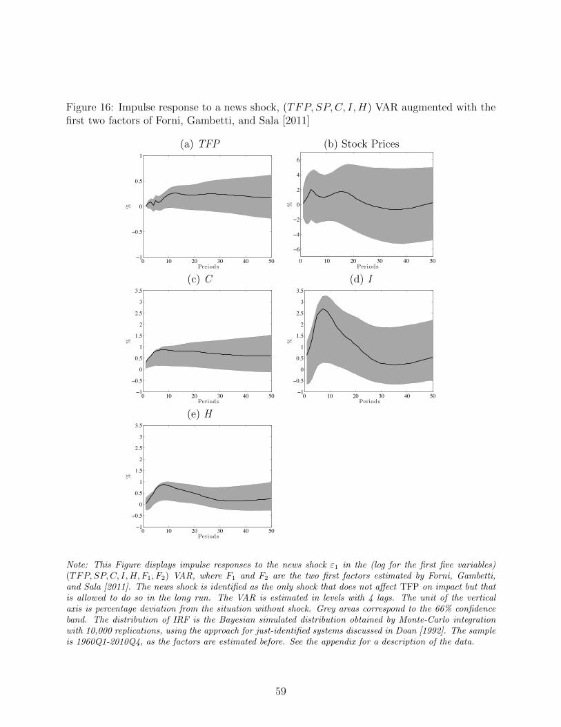
Figure 16: Impulse response to a news shock, (TFP, SP,C, I,H) VAR augmented with thefirst two factors of Forni, Gambetti, and Sala [2011]

(a) TFP (b) Stock Prices

0 10 20 30 40 50ï1

ï0.5

0

0.5

1

Periods

%

0 10 20 30 40 50

ï6

ï4

ï2

0

2

4

6

Periods

%

(c) C (d) I

0 10 20 30 40 50ï1

ï0.5

0

0.5

1

1.5

2

2.5

3

3.5

Periods

%

0 10 20 30 40 50ï1

ï0.5

0

0.5

1

1.5

2

2.5

3

3.5

Periods

%

(e) H

0 10 20 30 40 50ï1

ï0.5

0

0.5

1

1.5

2

2.5

3

3.5

Periods

%

Note: This Figure displays impulse responses to the news shock ε1 in the (log for the first five variables)(TFP, SP,C, I,H, F1, F2) VAR, where F1 and F2 are the two first factors estimated by Forni, Gambetti,and Sala [2011]. The news shock is identified as the only shock that does not affect TFP on impact but thatis allowed to do so in the long run. The VAR is estimated in levels with 4 lags. The unit of the verticalaxis is percentage deviation from the situation without shock. Grey areas correspond to the 66% confidenceband. The distribution of IRF is the Bayesian simulated distribution obtained by Monte-Carlo integrationwith 10,000 replications, using the approach for just-identified systems discussed in Doan [1992]. The sampleis 1960Q1-2010Q4, as the factors are estimated before. See the appendix for a description of the data.

59

announced tax cut with an anticipation horizon of 6 quarters gives rise to pre-implementation

declines in aggregate output, investment and hours worked. In contrast, aggregate consump-

tion is hardly affected by the announcement. Mertens and Ravn [2011] then propose a DSGE

model that can account for the impact of such tax policy shocks.

Once it it recognized that some tax and fiscal changes are anticipated, one should revisit

some of the previous VAR literature on fiscal shocks, as representations are likely to be

non fundamental, as illustrated by Leeper, Walker, and Yang [2008]. Ramey [2011] shows

that both professional forecasts and the narrative approach shocks Granger-cause fiscal VAR

shocks, implying that these shocks are missing the timing of the news, and therefore that

VARs do not properly estimate dynamic fiscal multipliers. Mertens and Ravn [2010] nicely

show that rational expectations models introduce restrictions on the non-fundamental roots

of the MA representations that allows to examine the sensitivity of SVAR based estimates

of the impact of fiscal shocks to news shocks. They use the fact that rational expectations

models imply that fiscal news are discounted at a constant rate, denoted the anticipation rate

by Ljungqvist and Sargent [2004]. This parameter can be used to recover the structural shock

of a fiscal VAR from its non fundamental representation. Leeper, Richter, and Walker [2012]

also identify two types of fiscal news—government spending and changes in tax policy. They

identify news concerning taxes through the municipal bond market, and news concerning

government spending through the Survey of Professional Forecasters. They then map the

reduced-form estimates of news into a DSGE framework. Gambetti [2012] measure fiscal

news as as the difference between the forecast of government spending growth over the next

three quarters made by the agents at time t (measured with the the Survey of Professional

Forecasters) and the forecast of the same variable made at time t. This variable is then

introduced in an otherwise standard VAR, and multipliers are found to be close to one.

Ben Zeev and Pappa [2013] identify US defense news shocks as shocks that best explain

future movements in defense spending over a five-year horizon and are orthogonal to current

defense spending. Those identified shocks induces significant and persistent increases in

output, consumption, investment, hours and the interest rate.

On a different perspective, Bruckner and Pappa [2013] examine the macroeconomic effects

of bidding for the Olympic Games using panel data for 188 countries during the period 1950-

2009. News about the Olympics makes output and investment surge already at the time of the

bidding. In unsuccessful bidding countries the agents’ optimism turns out to be unjustified

and, as a result, the economy returns to its original trend, while hosting economies enjoy

quantitatively large and significant positive effects from hosting.

Approaches where news events are directly observed and measured have an important

advantage over SVAR approaches as they tend not to be subject to the problem of non-

60

fundamentalness and therefore more likely to produce credible and less controversial results.

However, since these papers are not focused on business cycle issues and do not examine the

effects of technological news, their findings cannot be compared with the SVAR reviewed

in the previous subsection. One paper that is more closely related is Alexopoulos [2011].

Alexopoulos [2011] identifies dates where there are publications of books related to new

technological developments. She then uses these identified episodes to look at how the

economy reacts after a flurry of such technological dissemination. The main finding is that

TFP tends to increase with a substantial lag after such episodes, especially in the sectors

most likely to take advantage of such technological developments. Moreover, Alexopoulos

finds that economic activity tends to pick up after these news events, which supports the

idea that such positive news creates an expansion. Baron and Schmidt [2013] propose the

use of technological standardization as a novel indicator of technological change. They find

that standardization is an essential mechanism for revealing news about future movements

of macroeconomic aggregates as evidenced by the positive and immediate reaction of stock

market data to a technology shock. 58

4 Building and Estimating Structural Models with News

As we discussed in the previous section, the are several limitations of using VAR approaches

to evaluating the plausibility and importance of news driven business cycles. The main

alternative to VARs is to use fully specified dynamic general equilibrium models (either

estimated, calibrated or a mixture of both) to do model-based structural decompositions of

the sources of fluctuations. However, this alternative approach also has its limitations. As

is well known, when doing model-based structural decompositions the resulting inferences

depend critically on the assumed structure being right. If, for example, one adopts a dynamic

general equilibrium model where the underlying structure is such that the economy’s response

to news can never cause a generalized boom or bust – that is, the assumed structure is such

that news can never cause outcomes where consumption, investment and employment all

co-move positively together — then by construction such an approach will almost surely

attribute little importance to news in driving fluctuations, even if in fact they are relevant.

Therefore, before discussing the insights regarding news-driven business cycles obtained by

doing model-based structural decompositions, it is important to first ask the following two

questions: (i) in what types of dynamic general equilibrium models does news have the

58The results in Lucke [2013] can viewed as an intermediate steps between these two approaches. He usesinformation on patent filings in the US and Germany to see if the news shocks identified using a methodologysimilar to that used in Beaudry and Portier [2006] predicts patent filings. He finds they do and interprets thatas supporting the idea that the identified shocks contain news about subsequent technological developments.

61

potential to create business cycle-type fluctuations, and (ii) is the resulting class of models

reasonable? Once we clarify the answer to these two questions we will be in a better position

to discuss results from the model-based structural decompositions found in the literature.

4.1 In what DSGE environment can news creates business cyclefluctuations?

It appears intuitive to many that if agents in an economy wake up to news about new market

opportunities developing on the horizon, this will likely cause increased activity immediately

as agents both start to invest early to be ready when the new demand patterns materialize

and start to consume early as they feel richer. We have shown in the previous section

that such an intuitive pattern emerges from the VAR literature that aim at identifying

the effect of TFP news shocks. However, it turns out that such patterns are difficult to

generate within the confines of many of the simple dynamic general equilibrium models

used in macroeconomic literature. In particular, the difficulties arise on two fronts, which

we will refer to as the dynamic front and the static front. On the dynamic front, as we

shall show, in many simple dynamic models it is difficult for positive technological news to

cause an increased desire to invest today. On the static front, we will show that even if

positive technological news causes increased desire to invest, in many models this will not be

translated into increased consumption and investment today. Instead, it is most generally

be associated with either consumption or investment decreasing today.

To set the stage, let us begin by considering a very simple DSGE model in the RBC

tradition where (i) there is a representative agent who discounts the future at rate β with

per-period utility U(Ct, L− Lt) that depends on consumption Ct and leisure L− Lt, where

both consumption and leisure are normal goods ( Lt represent hours worked, and L is the

labor endowment), (ii) there is one final good that is produced with capital and labor using

a Cobb-Douglas technology θtKαt L

1−αt , where θt is a stochastic technology index and (iii)

the final good can be consumed or invested, with capital accumulation obeying Kt+1 =

(1− δ)Kt + It, where δ is the rate of depreciation and It is investment. In this environment,

what happens if today the representative household receives news that indicates that θ will

increase in q periods? As first hinted to in Barro and King [1984], and discussed in more

detail below, in such an environment it will never be the case that the news will lead to an

immediate increase in consumption, investment and employment. Moreover, under standard

calibrations, the news will not even lead to an increased desire to invest in anticipation of

the future technological change but will instead lead to a decrease in current investment and

employment. Hence, if someone chose to use such a framework to evaluate the importance

62

of news using model-based structural decomposition, then almost certainly the results will

be that news does not play a very important role. While that may be the right conclusion,

before drawing such a conclusion it is important to understand which assumptions cause

which difficulties for the news view of business cycles. To this end, we will present here a

framework which helps separate static difficulties and dynamic difficulties. An underlying

message of the section will be to show that standard DSGE models do not easily embody

the narrative of news-driven business cycles without significant modifications. This can be

interpreted in two ways: either the news view should be discounted as it does not fit into

mainstream models, or our standard business models are very restrictive and may need to

be generalized. Moreover, while the literature has recognized and offered solutions to the

static problem, this section will also emphasize a dynamic challenge that is somewhat less

recognized.

4.1.1 Addressing the static problem between news and business cycles

As mentioned previously, the mechanisms behind the news view can be divided into two dis-

tinct elements. First, there is the effect of news on agents’ and firms’ desire to invest in order

to be well placed to take advantage of future developments. We refer to this as the dynamic

element since it depends primarily on how agents’ perceptions about the future translate into

investment demand. Second, there is the notion that increased investment demand leads to

increased economic activity without creating negative co-movements between investment and

consumption. We refer to this second element as the static element since it looks at current

adjustment conditional on how agents perceive the future. In this subsection we want to

restrict attention to situations where (by assumption) news generates increased incentive to

invest, and focus on clarifying the conditions under which the increased investment demand

creates a boom. In order to make this distinction between the static and dynamic elements

operational, it is helpful to explicitly model the continuation value of capital in preferences.

In particular, let us start by assuming that we have a representative agent with a current

utility function given by U(Ct, 1−Lt) = U(Ct, Lt), where both consumption and leisure are

normal goods. Furthermore, let us summarize the agent’s perceived future utility by the

value function V (Kt+1,Γt+1). Here, Kt+1 is the stock of capital the agent will have next

period and Γt+1 is the state of the world next period.Let us be clear that we assume here

that VKS > 0 so that investment increases at the reception of the news. The features of

the model that can solve the static problem might not be sufficient to also sole the dynamic

problem: once the continuation value V is derived from the model fundamentals, it might

not satisfy VKS > 0. Some extra features will then be needed, that we discuss when looking

at the dynamic problem.

63

4.1.1.1 A one-sector economy: Consider a one-sector economy in which there is a

representative firm that hires labor and rents capital to produce output using the concave

production function F (Kt, Lt, θt). There is also a representative household whose objective

can then be stated as follows:

maxCt,Kt+1,Lt

U(Ct, Lt) + βE[V (Kt+1,Γt+1) | Ωt

],

s.t. Ct +Kt+1 = wtLt +Kt(1− δ + rt) + πt,

where wt and rt are the wage rate and the rental rate of capital, and πt are firm profits. Ωt

is the agent’s information set in period t which can for example include the current state of

technology θt and any signal St that the agent may have received as exogenous news. We

will refer to this simple macro model as the RBC structure. For ease of exposition it will be

helpful to define a continuation value function V (·) as follows

V (Kt+1, θt, St) = βE[V (Kt+1,Γt+1) | Ωt = θt, St

].

So the continuation value function of an agent is just the expectation of his value function

and therefore depends on the stock variables one brings in to next period, which in the RBC

structure is only Kt+1, and on his information set Ω which he used to form his expectations.

The information set in this case is comprised both of the current state of technology θt as

well as extra information arrived in the form of news denoted by St. Although in general

the news could be multi-dimensional, we will assume for now that it corresponds simply to

a scalar where a higher value of St corresponds to more productive technology in the future.

While the agent’s continuation value function depends on future utilities U(Ct+i, 1−Lt+i) and

future production possibilities, for now we will bypass thinking about these links explicitly

and instead assume that an increase in the signal St increases the desire to invest by assuming

that∂2V (Kt+1, θt, St)

∂Kt+1∂St> 0.

That is, we assume that an increase in the signal increase the perceived marginal value of

entering next period with greater capital. We are not being specific about the type of tech-

nological change that the news St could be forecasting or why it would cause an increase in

the marginal value of acquiring capital. The conditions under which an expected technology

improvements cause the perceived value of holding capital to go up will be discussed in the

subsection under the heading of dynamic challenge. By taking this property of the value

function as given, and assuming that VKK(·) ≤ 0, we can focus solely on how the economy

adjusts immediately to an increased desire to hold capital, which is a static problem, without

needing to get entangled with dynamics. In other words, we study the temporary equilib-

rium of the economy for given expectations, those expectations being embedded into the V

64

function. The Walrasian equilibrium quantities for this problem, Kt+1, Ct and Lt, can then

be represented as the solution to the three following equations:

∂V (Kt+1, θt+1, St)]

∂Kt+1

= UC(Ct, Lt), (39)

FL(Kt, Lt, θt) =−UL(Ct, Lt)

UC(Ct, Lt), (40)

Ct +Kt+1 = F (Kt, Lt, θt) + (1− δ)Kt. (41)

Equation (39) is the usual intertemporal Euler equation, (40) is the intratemporal consumption-

leisure decision (the labor market equilibrium in a decentralized version) and (41) is the

economy resource constraint. This setup allows us to examine how Kt+1, Ct and Lt change

in response to an increase in St by performing a simple comparative static exercise on this

three-equation system. It is here that we can see what we refer to as the static challenge for

news-driven business cycles. In this setup, if the news increases the desire to invest (which we

are assuming it does by assumption) then it will lead to a decrease in consumption; that is,

the news cannot cause a generalized boom with both consumption and investment increasing.

This property of the RBC structure was first noted in Barro and King [1984] and made more

explicitly related to news (or expectations) in Beaudry and Portier [2007]. The property can

be seen directly from equation (40): the intratemporal labor market equilibrium condition.

From this equation, under the assumption that consumption and leisure are both normal

goods, it can be directly verified, by simply taking a total differential holding capital and

technology constant, that consumption and employment cannot move in the same direction.

Hence consumption and investment cannot move in the same direction. This is the precise

point made by Barro and King [1984].

Why is Barro and King’s [1984] observation a difficulty for a news view of business

cycles? To the extent that we interpret the previous VAR result as suggesting that in

response to news the economy expands with both consumption and investment increasing

(at least weakly) throughout the substantial period where technology has not yet increased,

then such features cannot be generated within the structure. Furthermore, even if one is

unsure about the VAR results, but one believes that news may offer a reasonable theory

of the business cycle, then it is useful to identify conditions under which news shocks do

not create negative co-movement between consumption and investment. Accordingly, we

take this static difficulty as a challenge for news-driven business cycles and we proceed here

to discuss the different solutions proposed in the literature. However, before looking at

different possibilities we want to first clarify the limited role played by income effects in

creating the difficulty, since there appears to be some confusion on this point. In fact, Barro

and King’s [1984] result is not at all driven by income effects on labor supply. If we exclude

65

income effects on labor supply, for example by assuming that the utility function is of the

form U(Ct − τ1L1+τ2t ), where τ1 and τ2 are positive parameters, then we get the exact same

difficulty. 59 Actually, the problem becomes even simpler in the absence of income effects

on labor supply since with such preferences, technology and preferences pin down output,

independently of the value function. Hence in this case news can only cause purely off-setting

changes in Ct and It, keeping the sum constant.

In response to this static challenge, the literature has proposed several departures from

the simplest RBC-style structure to explain why news shocks do not necessarily imply an ini-

tial phase of negative co-movement between investment and consumption. These departures

range from modest to substantial. We will start be discussing changes that to do not require

modifying the arguments of the value functions, and then discuss those that do require such

changes. 60

4.1.1.2 Changing preferences: One simple departure that overcomes Barro and King’s

[1984] problem is to allow consumption or leisure to be inferior goods. In particular, if

we assume that consumption is an inferior good then the difficulty does not necessarily

emerge. Moving away from the normality assumption about goods may at first pass appear

unreasonable, but Eusepi and Preston [2009] argue that the representative agent’s preferences

should be thought of as an aggregation of preferences for workers and non-workers (under

complete insurance) and that in the presence of non-convexities61 the resulting aggregate

preference may have consumption as an inferior good even if the preferences of the underlying

agents have both consumption and leisure as normal goods. Using this idea they then show

that in a reasonably calibrated model, the arrival of news can lead to an immediate increase

in both consumption and investment. Eusepi and Preston [2011] use a similar framework to

show how learning dynamics create shifts in expectations and generate business cycles. 62

59This should not be surprising as these preferences were not ruled out by our assumptions.60Wang [2012] has proposed a review of the models that generate positive co-movements. Those properties

are nicely presented in terms of labor market structure (upward or downward sloping labor supply, outwardsshifting labor demand following a technological news). Eusepi [2009] shows that in a one-sector model witheconomy-wide externalities, there is a tight connection between positive co-movements and indeterminacy,as conditions for positive co-movements are necessary to obtain indeterminate equilibria. That connectionis broken in two-sector economies. Guo, Sirbu, and Suen [2012] show that good technological news actuallycreates an aggregate recession in Eusepi [2009] simple on-sector model. Guo, Sirbu, and Weder [2012] alsodiscuss the link between positive co-movements and indeterminacy. Sorge [2012] show that news-drivenmodels and indeterminate equilibrium economies with i.i.d. fundamentals are observationally equivalent.

61Eusepi and Preston [2009] assume that participating to the labor market entails a fixed cost.62Zhang [2012] study the stability under learning (E-stability) of Jaimovich and Rebelo’s [2009] model,

and shows that when agents do not observe current state variables when forming expectations, the rationalexpectations equilibrium is not learnable for calibrated parameter values capable of generating news-drivenrecessions.

66

In a different take on this idea, Karnizova [2010b] suggests that news directly affects labor

supply which relaxes the resource constraint allowing both investment and consumption to

increase. This is achieved by assuming that financial wealth enters the utility function. She

calls this effect the Spirit of Capitalism and shows how news can cause consumption and

investment to grow on impact. While these are interesting ideas, they both imply that the

initial expansion following news is due to a labor supply effect instead of increased demand

for labor. This implies that real wages should be counter-cyclical. Again, to the extent that

the VAR results are informative about the effects of news, such an implication may be at odds

with the data as real wages appear to be weakly increasing in response to news. However,

more exploration along this front will be needed to assess the validity of such mechanisms.

Finally, Malkhozov and Shamloo [2012] introduce non separable Epstein and Zin [1989]

preferences in an RBC model with news shocks, and show that it creates a persistent pre-

dictable component in consumption growth, that is often referred to as long-run risk in

the finance literature(Bansal and Yaron [2004]). Although the model does not allow for

variable labor, so that consumption and investment move in opposite direction following a

technological news, an extension with variable labor supply could potentially solve the static

problem.

4.1.1.3 Allowing for sticky prices and accommodative monetary policy: An-

other avenue discussed in the literature for overcoming the ‘static problem” associated with

news is to allow for sticky nominal prices. When prices are fixed, the very mechanism of IS-

LM imply that C, Y and H all increase following an exogenous increase in I, that is driven by

“animal spirits”. When prices are not fixed but sticky, this avenue has been pursued in many

papers including Christiano, Ilut, Motto, and Rostagno [2010], Khan and Tsoukalas [2012],

Lorenzoni [2009], Auray, Gomme, and Guo [2009], Fujiwara, Hirose, and Shintani [2011],

Jinnai [2013a] and Blanchard, L’Huillier, and Lorenzoni [2009]. However, as we shall show,

it is not sticky prices in and of themselves that is needed to overcome the static problem,

but it is sticky prices combined with a particular type of monetary policy. In effect, what is

required is that monetary policy be sufficiently accommodative to news. To understand how

news and sticky prices interact on impact, consider a slight generalization of the one-sector

framework where agents can now hold money and capital, and where we assume that the

nominal price of goods is predetermined. Money is directly introduced in the agents’ value

functions as a short hand for its eventual liquidity services. The representative household’s

67

problem can then be stated as

maxCt,Kt+1,Mt+1,Lt

U(Ct, Lt) + βE[V (Kt+1,Mt+1, θt, St),

s.t. Ct +Kt+1 +Mt+1

Pt= wtLt + (1− δ + rt)Kt +

Mt

Pt+ πt +

τtPt,

where Pt is the price of goods in terms of money, and τt is an exogenous money transfer with

next period’s money supply given by Mt+1 = Mt + τt. Money balances are directly assumed

to enter the function V (·) with V22 < 0. To give sticky prices their full force, we will assume

that Pt does not react to news. Without loss of generality we can therefore set Pt = 1. To

complete the model we need to specify how the money transfer τt is determined. Since the

nominal price of goods is assumed to be fixed, a simple monetary rule is to have τ react to

deviations of output for a long run average according to:

τt = α(Yt − Y )

where Y is a reference rate of output, Yt = Ct + It and α governs the extent to which

monetary policy either leans against demand shocks or amplifies them: if α < 0 monetary

policy leans against demand shocks; if α > 0 then monetary policy is pro-cyclical in the

sense of expanding when demand is high. The equilibrium levels of consumption Ct and

investment It are then determined by the set of equations

VK(Kt+1,Mt+1, θt, St) = VM(Kt+1,Mt+1, θt, St),

UC(Ct, Lt) = VK(Kt+1,Mt+1, St),

F (Kt, Lt) = Ct +Kt+1 − (1− δ)Kt,

Mt+1 = Mt + α(Ct + It − Y ),

It = Kt+1 − (1− δ)Kt.

Now consider the arrival of a signal St that increases the marginal value of holding capital

(VKS > 0). How does this affect investment and consumption? To simplify the analysis,

assume that U(Ct, Lt) is separable between consumption and employment, and assume that

V (Kt+1,Mt+1, St) is separable between capital and money with St only affecting the value

of capital. In this case, investment increases but the response of consumption is ambiguous

as it hinges on the sign of α in the monetary rule. If α < 0 then consumption decreases

in response to news that increases the demand for investment. If α = 0 then consumption

is unchanged. Only if α > 0 do we have both consumption and investment increasing in

response to the news. The positive co-movement arises because monetary policy becomes

expansionary in response to the news. Hence, sticky prices offers an avenue to overcome the

68

static problem with news-driven business cycles, but the mechanism is somewhat fragile since

it relies crucially on how monetary policy reacts to news. 63 For example, in a simple New

Keynesian model 64 in which price stickiness is the only distortion and without cost push

shocks, the optimal monetary policy replicates the flex price allocations. The model is then

a standard RBC model (without capital), and consumption and hours worked always move

in opposite directions following a news shock. It is only when monetary policy is suboptimal

that C and H can co-move positively. 65

4.1.1.4 Adopting a two sector structure: One of the reasons that increased invest-

ment demand leads to decreased consumption in an RBC model structure is due to the

one-sector assumption. With only one sector, investment goods and consumption goods are

perfect substitutes 66 and therefore it is generally optimal to reduce one when there is in-

creased demand for the other. In contrast, with a two-sector model, where factors are specific

to the sector, investment and consumption are not direct substitutes and accordingly it turns

out to be much easier to generate increased investment in response to news without having

consumption decrease. To see this, let us slightly extend the previous setup to allow for two

sectors, maintaining for now the assumption of a representative household. The first sector

is the consumption sector with Ct = F (KCt , L

Ct ; θCt ), where LCt is the level of employment in

the sector, KCt is the capital used in the sector, θCt is a technology index in the consumption

sector and F (·; θC) is a concave function. The second sector is the investment sector with

IIt + ICt = G(KIt , L

It ; θ

It ), where IIt and ICt are the investments directed to the accumulation

of capital in the investment and consumption sectors, respectively. KIt and LIt are sector-

specific factors, and G(·; θI) is a concave function. The accumulation of capital is given by

KIt+1 = IIt +(1−δ)KI

t and KCt+1 = ICt +(1−δ)KC

t . The household’s utility is assumed to take

the form U(Ct, LCt , L

It ), where we allow for the possibility that labor from the two sectors are

63Karnizova [2010a] study a simple New Keynesian monetary business cycle model with news shocks andsunspot ones when monetary policy is passive or active. Another model that also leads to countercyclicalmarkups is proposed by Pavlov and Weder [2013]. Using Gali’s [1994] monopolistic competition frameworkin which investment and consumption have a different price elasticity of demand, they show that news shocksimply countercyclical markups and can therefore generate positive co-movements.

64See for example chapter 3 in Galı’s [2008] book.65Guo [2007] explores the optimal response of a central bank when a news shock hits the economy in

a two-sector model with price rigidities in each of the non-durable and durable sectors. Blake [2012] alsoshows that monetary policy can be designed to mitigate the effects of news shocks on output and inflation.Romero Alom [2012] presents a simple New-Keynesian model in which it is optimal to include asset prices inthe Taylor rule when there are news shocks. On monetary policy with news shocks, see also Jinnai [2013b].

66If capital is fully mobile between the two sectors, then the Walrasian equilibrium in the two-sector modelbehaves similar to that of the one-sector. In particular, in response to news that increases the marginal valueof holding capital, the production of the consumption good will decrease. See Beaudry and Portier [2007]for details.

69

imperfect substitutes in preferences. Finally, as before, we summarize the agent’s perception

about the future as given by the continuation value function V (KIt+1, K

Ct+1, θ

It , θ

Ct , St), so

that the agent’s problem can be stated as

maxCt,KC

t+1,KIt+1,L

Ct ,L

It

U(Ct, LCt , L

It ) + V (KC

t+1, KIt+1, θ

Ct+1, θ

It+1, St),

s.t. Ct + P It (KC

t+1 +KIt+1) =

wCt LCt + wItL

It +KC

t (P It (1− δ) + rCt ) +KC

t (P It (1− δ) + rIt ) + πCt + πIt ,

where P It is the price of investment goods and the superscripts C and I indicate the con-

sumption and investment sectors. In this setup, suppose the representative household re-

ceives news about future technological change that leads him to believe that the marginal

value of holding capital – either in one or both sectors – increases. What happens to con-

sumption and employment in each sector assuming a Walrasian equilibrium? In contrast to

the one-sector model, consumption does not necessarily decrease in this case. The easiest

case to see this is the one where U(Ct, LCt , L

It ) is separable in its three arguments. 67 In such

a setup, consumption and employment in the consumption sector are determined by the two

equations:

−ULC (LCt )

UC(Ct)= FLC (KC

t , LCt ),

Ct = F (KCt , L

Ct ).

Under the assumption of separability in the utility function, these two equations can be

solved independently of the decisions in the investment sector, and therefore independently

from any change in the information set Ωt which would be affected by news. In other

words, employment and output in the consumption sector do not respond to news. In

contrast, employment in the investment goods sector will generally be directly affected by

news. Investment decisions and employment in that sector are determined by the set of three

equations:

GLI =−ULIVKI

,

GLI =−ULIVKC

,

G(KIt , L

It ) = KI

t+1 − (1− δ)KIt +KC

t+1 − (1− δ)KCt .

Therefore, if news increases either VKI or VKC , then it will lead to increased employment and

output in the investment sector. Hence, in such a two-sector structure, news that increases

67Or when it can be written as U(Ct−hC(LCt )−hI(LIt )), where U(·) is a concave function and where thefunctions h(·) are convex

70

demand for investment does not give rise to a negative co-movement between consumption

and investment or, stated differently, the static problem with news seen in the one-sector

model does not arise. However, in the separable case, since consumption neither increases

nor decreases in response to news, it may be considered a knife-edge result.

Recall from the VAR results that consumption seemed to increase immediately in re-

sponse to news, so it would be interesting to know if both consumption and investment

can respond positively to news in the Walrasian equilibrium of a two sector model. It is

actually possible to have both consumption and investment strictly increase in response

to news in this setup but, if we maintain a representative agent assumption, it requires

quite uncommon non-separability assumptions for the utility function U(Ct, LCt , L

It ).

68 A

more promising avenue for having both consumption and investment increase in response

to news in a two-sector framework is, according to Beaudry and Portier [2013], to depart

from the representative agent setup and adopt a framework with static gains from trade be-

tween heterogenous agents. It is shown there that, in a two sector model where households

are specialized in the sense of being attached to one sector for their employment 69 , then

increased demand for investment goods will most often be associated with an immediate

increase in aggregate consumption as those employed in the investment goods sector will

use part of their increased income to buy consumption goods.Luttmer [2013] also explores

a model with expectation revisions in a multi-sectoral structure with consumption and in-

vestment sector. The consumption sector is labor intensive whereas the investment sector

is manager incentive. When a good news hits, consumption increases, which increases the

labor wage via a Stolper-Samuelson effect, which in turn increases hours worked. In the

Luttmer’s [2013] model, such a consumption and hours boom is nevertheless accompanied

by a drop in investment. To summarize, moving from a one-sector to a two-sector framework

greatly reduces, and can even overcome, the static problem of having news cause negative

co-movement between consumption and employment.

4.1.1.5 Current Employment in the Value Function: A fourth avenue which has

been suggested as a way to solve the negative co-movement problem between consumption

68For example if the U(Ct, LCt , L

It ) = ln(Ct − τ1(LIt )

1+τ2) − ν · LCt then an increase in VKI or VKC willlead to a simultaneous increase in consumption and total investment. Alternatively, if we summarize thetwo sector production possibilities by (Cσt + Iσt )

1σ = F (Kt, Lt) with σ < 1, we can also get news to lead

to an increase in both consumption and investment, as shown in Beaudry and Portier [2007] for details.Katayama and Kim [2012] have built a two-sector model whose key elements are frictions in intersectorallabor mobility and non-separable preferences in consumption and leisure, along with adjustment costs toinvestment and variable capital utilization. That model is able to generate comovements in response to bothcontemporaneous shocks and news shocks about fundamentals.

69This result also relies on incomplete insurance markets so that the economy does not aggregate to arepresentative setup.

71

and investment is to have the level of past employment directly enter the value function,

with the property that news increases the marginal value of past employment. Consider a

model in which the household problem can be written as follows:

maxCt,Kt+1,Lt

U(Ct, Lt) + V (Kt+1, Lt, θt, St),

s.t. Ct +Kt+1 = wtLt +Kt(1− δ + rt) + πt,

where we assume that VKL ≥ 0, VLS > 0 and VLL ≤ 0. The simplest rationale for why

past employment may enter the value function this way is adjustment costs to labor. In

the presence of convex adjustment costs for labor, current news that anticipates later em-

ployment growth will directly favor employment today as to reduce the adjustment costs.

This increased labor demand then leads to increased production, which can be split between

consumption and investment. In effect, the intratemporal consumption-leisure decision (40)

is now given be the following

−UC(Ct, Lt)FL(Kt, Lt, θt) = UL(Ct, Lt) + VL(Kt+1, Lt, θt, St)

Fully differentiating the above equation and assuming separability of utility for the ease of

exposition, one obtains

(UCFLL + ULL + VLL)︸ ︷︷ ︸−

dLt = −UCC︸ ︷︷ ︸+

dCt +−VLK︸ ︷︷ ︸−

dKt+1 +−VLS︸ ︷︷ ︸−

dSt

As it is clear from this equation, a positive news dSt that increases investment (dKt+1 > 0)

can move upwards Ct and Lt.

Hence, the presence of convex adjustment to labor offers a very simple resolution of the

static problem with news. However, there are a few potential drawbacks of this mechanism.

First, much of the microeconomic evidence suggests that labor adjustment costs are either

fixed or linear, not convex. Second, to the extent that the microeconomic literature does

find evidence of convex adjustment costs to labor, they tend to be small which means that

in response to news this mechanism may be quantitatively too weak to offset the negative

co-movement problem. Third, with convex labor adjustment costs, the response when agents

discover that they have been accumulating too much capital will no longer cause an abrupt

fall in employment – which is a feature we believe is desirable. Instead the adjustment will

tend to be gradual.

The papers by Den Haan and Kaltenbrunner [2009] and Gunn and Johri [2011] implicitly

exploit ideas that work somewhat similarly to convex adjustment costs to labor but offer

plausible mechanisms. In particular, Den Haan and Kaltenbrunner [2009] explored the effects

of news in a search and matching model. The search frictions give rise to a mechanism by

72

which news leads firms to want to post vacancies immediately as to have sufficient employed

workers when the expected demand forecasted by the news is eventually realized. This is

similar in spirit to convex adjustment cost to labor, but with better microeconomic support.

Den Haan and Kaltenbrunner [2009] showed that the static problem associated with news

can be overcome in such a setup. 70 In a quite different spirit, Gunn and Johri [2011] have

suggested that learning by doing creates a reason why news may directly affect labor demand

today. In response to news, it becomes profitable to hire more workers today as to have more

human capital built up through learning-by-doing when new demand arises. They show that

such a learning-by-doing mechanism can also overcome the negative co-movement problem,

and it works essentially by giving a dynamic value to current employment. 71

In summary, we have defined the static challenges associated with news as the difficulty of

getting both consumption and investment to increase when agents get information regarding

a future technology improvement. While this problem is present in the Walrasian equilibrum

of a one-sector representative agent model, we have shown that the problem can be overcome

by departing from such a simple model. In particular, we have discussed, among others,

how sticky prices, adjustments costs to labor and adopting a two-sector formulation can

mitigate the tendency of increased investment to cause a decrease in consumption. While the

different mechanisms presented each have their strengths and weaknesses, further empirical

exploration is needed to identify which path offers a more plausible solution. 72

4.1.2 The dynamic challenge of news and business cycles

As mentioned previously, there are two central elements to the news view of business cycles

that we have set out. Firstly, there is the idea that news about future developments in

the economy create incentives for either firms or individuals to start investing immediately

in preparation for the eventual changes. Second is the idea that the increased investment

demand induced by news stimulates economic activity in a way that generates an aggregate

boom in both consumption and investment. One challenge for a news theory of business

cycles, especially one based on technological news, is to present plausible but simple DSGE

models that capture these two features. In the previous section we have discussed what we

have referred to as the static challenge; that is, identifying environments where increased

70In their survey on the news shocks literature, Krusell and McKay [2010] also propose a simple searchmodel that generate cycles driven by news shocks.

71See also Qureshi [2009] for a similar mechanism.72All the mechanisms we have discussed in this section have assumed a production structure which is not

subject to increasing returns-to-scale. However, increasing returns to scale offers an alternative mechanismwhich can explain how changes in expectations can lead to increases in both consumption and investment.In fact, as shown in Benhabib and Farmer [1994], in the presence of increasing returns to scale the economycan exhibit business cycles driven by self-fulfilling beliefs.

73

investment demand can lead to aggregate booms in both investment and consumption. In

this section we want to discuss a dynamic challenge, that is, clarifying how and when news

of future technological improvements creates increased incentive to invest today. In terms

of our notation, the dynamic challenge refers to presenting environments where the agents’

continuation value functions have the property that positive technological news increases the

marginal value of bringing capital into the future. While the literature has recognized the

static challenge related to the co-movement problem and suggested solutions, the dynamic

challenge has been much less discussed or recognized. 73 To highlight the nature and extent

of the dynamic challenge, we begin by discussing it within the context of a two-sector model,

since such structure allows us to consider separately the effects of expected technological

improvements in either the consumption or the investment sector. Note that the one-sector

model is just a special case of our two-sector setup.

4.1.2.1 Two-sector case: Let us return to the two-sector model we have previously in-

troduced in this section, where F (KCt , L

Ct , θ

Ct ) is the production function in the consumption

sector and G(KIt , L

It , θ

It ) is the production function in the investment sector. For simplicity,

let us assume that θjt+1 = ρθjt + εjt with j ∈ C, I and where εjt is an innovation that affects

technology at time t+1 but is known by agents through news at time t. If the representative

agent’s period utility is given by U(Ct, LCt , L

It ), competitive allocations can be obtained from

a social planner problem and the planner value function at time t can be defined as

V (KCt , K

It ,Σt) = max

Ct+i,KCt+1+i,K

It+1+i,L

Ct+i,L

It+1+i

∞i=0

Et

∞∑i=0

U(Ct+i, LCt+i, L

It+i),

s.t. Ct+i = F (KCt+i, L

Ct+i, θ

Ct+i),

(KCt+1+i − (1− δ)KC

t+i) + (KIt+1+i − (1− δ)KI

t+i) = G(KIt+i, L

It+i, θ

It+i),

where Σt = (θCt , θIt , ε

Ct , ε

It ) is the vector of current exogenous states. The issue we want to

examine is how do changes in news represented by changes in εC and εI affect the marginal

value of holding capital. Using the envelope condition, the marginal value of having capital

in period period t+ 1 can be expressed, for each type of capital, as

VKC (KCt+1, K

It+1,Σt+1) =UC(Ct+1, Lt+1, L

It+1)FKC (KC

t+1, LCt+1, θ

Ct+1)

+(1− δ)

GLI (KIt+1, L

It+1, θ

It+1)− ULI (Ct+1, L

Ct+1, L

It+1)

73One paper that emphasizes and addresses this dynamic challenge is Dupor and Mehkari [2013].

74

and

VKI (KCt+1, K

It+1,Σt+1) =

−ULI (Ct+1, Lt+1, LIt+1)

GLI (KIt+1, L

It+1, θ

It+1)

((1− δ)

+GKI (KIt+1, L

It+1, ρθ

It+1)).

Let us now follow some standard parameterizations in the literature by assuming that

the utility function is of the form lnCt− ν · (LCt +LIt ) and that the production functions are

Cobb-Douglas: F (·) = θCt (KCt )α

C(LCt )1−α

Cand G(·) = θIt (K

It )α

I(LIt )

1−αI . The linearity in

the disutility of work is not important but will make our argument more transparent. Under

these two parametric assumptions, the expected marginal values of bringing capital into the

next period (that is, the derivative of the continuation value function) can be expressed as

VKC (KCt+1, K

It+1,Σt+1) = β

(αC

KCt+1

+ν(1− δ)Et(LIt+1)

αI

(1− αC)(θIt + εIt )(KIt+1)

αI

), (42)

VKI (KCt+1, K

It+1,Σt+1) = β

(ν(1− δ)Et(LIt+1)

αI

(1− αC)(θIt + εIt )(KIt+1)

αI+νEt(L

It+1)

KIt+1

). (43)

There are several aspects we want to emphasize about how these particular parametric as-

sumptions on utility and production functions restrict the incentive to hold capital. First,

note that the only endogenous variable as of time t + 1 to appear in either (42) or (43)

is employment in the capital goods sector. Second, the information related to future tech-

nological progress in the consumption sector εCt does not appear anywhere in these two

expressions except potentially through the expectation of LIt+1. Finally, the information on

technological progress in the investment sector appears directly only in the denominator of

these expressions. Under these parametric assumptions, we can see why it will be very dif-

ficult for positive technological news to create an incentive to hold more capital. Actually,

it can be shown that under these assumptions, news about technological improvements in

the consumption goods sector never increases the marginal value of holding capital since it

does not affect LIt . Hence this type of parameterization entirely rules out the possibility that

expected technological improvements in the consumption good sector creates incentives for

agents start accumulating capital immediately to take advantage of the news. 74 For tech-

nological news regarding the investment sector, such a general statement is harder to obtain.

Nonetheless, we have found the effect of positive news to almost always decrease the value

of holding capital. This later property should not be surprising, as expected technological

74This effect is closely related to the fact that in a Lucas tree model, an increase in future productivityof trees does not increase the price of the tree in terms of the consumption good when utility is of the formU(Ct) = ln(Ct).

75

improvement in the capital goods sector creates a very intuitive incentive to postpone buying

capital now when one knows that improvements in the sector are imminent. 75

What to take from these observations on the continuation value function? On the one

hand, if one is wedded to standard parameterizations of business cycle models, these observa-

tions suggest that positive technological news is unlikely to be an important driving force in

investment demand. On the other hand, if one believes the business press, which commonly

suggests that investment demand is an important driver of business cycles, then it favors

considering models which allow substantial departures from standard parameterization of

DSGE models. In the latter case, there are two avenues that appear to us to be most

promising. The first relates to reducing the sensitivity of the stochastic discount factor.

In the above setup, one of the main reason that positive news about future technology

is not associated with increased incentives to invest is that it simultaneously leads to an

increased interest rate that fully offsets the expected increase in the marginal productivity

of capital. There are potentially many avenues to reduce the effect of news on the interest

rate including: changing the preference structure 76 , allowing for heterogeneous agents with

some agents having inter-temporal elasticity of substitution greater than one, or adopting

a sticky price setting with lax monetary policy. A second avenue for obtaining VKεI > 0 is

to consider production structures where technological news has a much greater effect on the

marginal product of capital in comparison to the average product of capital. With a Cobb-

Douglas structure, technological change causes the average product of capital to increase

in the same proportion as the marginal product of capital, and the expectation of such

a change is therefore associated with a substitution effect (induced by the increase in the

marginal product of capital) that favors more investment to be offset by a large income effect

(induced by the increase in the average product of capital) that favor postponing investment.

Departing from a Cobb-Douglas structure can change the relative size of the effects. For

example, if one adopts a CES structure where labor and capital are very complementary and

the news relates to labor augmenting technological change, the news will then increase the

marginal product of capital more than the average product. 77 and this will create incentives

to invest. Alternatively, if capital and labor are very substitutable and the news relates to

capital augmenting technological change, the effect of the news on the marginal productivity

of capital will be greater than the average effects thereby again creating clear incentives to

75Note that this structure implicitly nests a more standard one-sector model when one assumes thatαC = αI , and accordingly implies that positive technological news in a one-sector model with Cobb-Douglastechnology and log preferences for consumption will generally decrease the incentive to invest, not increasethem.

76In the model of Section 2, we completely eliminate this interest rate effect by allowing for home produc-tion.

77This is the mechanism used in Beaudry and Portier [2004].

76

invest in response to the news as the substitution effect will dominate the income effect. A

third way to proceed is to consider technological change more in a Schumpeterian tradition

where new opportunities tend to displace old ones making the private gains to investing much

greater that the social gain (which drives the income effect). 78 Accordingly, in response to

news that favors creative destruction, the return to new investment can be high even if the

net effect on output can be low. Such an avenue appears promising but it doesn’t fit easily

into the standard DSGE framework.

4.1.2.2 Jaimovich and Rebelo’s [2009] Approach: We have emphasized two types

of challenges facing news-driven business cycles when trying to embed the idea within a

simple DSGE structure. These challenges arise largely because we have been wanting to

build a model where news-driven booms reflect a period where agents have an incentive to

accumulate or install new capital early on as to be ready when future demand materializes.

However, this may be the wrong focus. Instead, it may be that good technological news in

fact reduces the incentives to accumulate capital and instead favors a rapid depreciation of

the current capital stock through increased utilization. In such a case, the induced increase

in utilization could itself cause a boom. This alternative view of how news may affect the

economy is most clearly captured in the work of Jaimovich and Rebelo [2009], and has the

attractive feature that it can easily overcome some of the challenges faced by our preferred

perspective which relies on news increasing the incentive to accumulate capital during the

anticipation stage.

In Jaimovich and Rebelo [2009], news is introduced in a quite standard one-sector repre-

sentative agent business cycle model. The model includes two important elements: variable

capacity utilization and adjustments costs to investment, 79 which are both quite reasonable

assumptions. These two elements interact in a way that can give rise to news-driven busi-

ness cycles where the main effect of the news is to encourage quicker capital depreciation

today as opposed to increasing the incentive for capital accumulation. The quicker capital

depreciation results from an increased utilization rate which favors producing more today

and thereby causing a boom. Since Jaimovich and Rebelo [2009] study the properties of

the Walrasian equilibrium, equilibrium outcomes can be presented as the solution to a so-

cial planner’s problem. In particular, the social planner’s problem in their setup takes the

78See Beaudry, Collard, and Portier [2011] for an example along these lines.79Jaimovich and Rebelo [2009] also emphasize a preference structure which minimizes wealth effects on

labor supply. While this feature is important for the quantitative aspects of their model, it is not central toits qualitative properties and therefore we will not emphasize it much here.

77

following form

maxCt+i,Kt+1+i,Lt+i,µt+i∞i=0

Et

∞∑i=0

U(Ct+i, Lt+i),

s.t Ct+i +Kt+1+i = F (µt+iKt+i, Lt+i, θt+i) + (1− δ(µt+i))Kt+i −ψ

2(It+i − It−1−i)2,

It+i = Kt+1+i − (1− δ(µt+i))Kt+i,

where the depreciation rate of capital δ(µt+i) is an increasing function of utilization rate

µt+i, and where ψ(It+i − It−1−i)2 captures the adjustment cost to investment. 80 81 Let us

again assume that agents get news one period in advance about θ, where θt+1 = ρθt + εt,

with εt being the news received at time t about technology at t+1. To simplify this problem,

and allow easy comparison with the framework we have already set out, it is useful again to

summarize the future using a continuation value function. Given this setup, the expected

continuation value function will depend on the capital stock coming into the period, last

period’s investment rate, last period’s state of technology and the news (regarding innovation

in next period’s technology), so that the optimization problem becomes:

maxCt,Kt+1,It,Lt,µt

U(Ct, Lt) + V (Kt+1, It,Θt, εt),

s.t. Ct +Kt+1 = F (µtKt, Lt, θt) + (1− δ(µt))Kt −ψ

2(It − It−1)2,

It = Kt+1 − (1− δ(µt))Kt.

The equilibrium outcomes for Ct, Kt+1, µt, Lt, It is then given implicitly as the solution to

the following equations plus the two constraints above

Fµ(µtKt, Lt, θt) = Ktδµ(µt)VK(Kt+1, It,Θt, εt)

UC(Ct, Lt),

VI(Kt+1, It,Θt, εt)

UC(Ct, Lt)) = ψ(It − It−1) +

(1− VK(Kt+1, It,Θt, εt)

UC(Ct, Lt)

),

−UL(Ct, Lt)

UC(Ct, Lt)= FL(µtKt, Lt, θt).

The first of these equations is the optimality condition for the setting of the utilization rate

µt. It states that the utilization rate should be chosen such that its marginal productivity

is equal to the marginal cost, where this cost is high if VK(·) is high. So the effects of news

80In Jaimovich and Rebelo [2009], news about both labor-augmenting technological change and investment-specific technological change are allowed. For simpler exposition, here we focus only on news about labor-augmenting technological change.

81As in the case of labor adjustment costs, the empirical literature suggests that non-convex costs tocapital adjustment are also important (Cooper and Haltiwanger [2006]). Furthermore, the flow specificationof adjustment costs (cost to the change of investment and not of capital) is also quite debatable, as it seemsnot to be found significant in empirical studies (Groth and Khan [2007])

78

on utilization depends on how εt affects VK(·). In this model, it is the case that positive

news about tomorrow’s technology (i.e., an increase in εt) will generally be associated with

a fall in VK(·) – because the economy is more productive in the future. In other words,

good technological news in the setup proposed by Jaimovich and Rebelo [2009] reduces

the incentives of agents to accumulate capital. However, due to the adjustment costs to

investment, it creates an incentive to increase investment. 82 These two forces may at

first pass appear contradictory, but with variable capacity utilization the two incentives

can be met by increasing capacity utilization in response to the news, thereby reducing

the capital shock while simultaneously having high investment. Hence, the first-order effect

of positive news in this setup is to increase capacity utilization. Since labor is assumed

to be complementary to capital services this leads to an increase in labor demand and an

expansion in the economy. 83 Because VK(·) is lowered by the news and VI(·) is increased,

the expansion will be associated with an increase in both consumption and investment. The

more difficult effect to sign in the model is the effect of the news on the capital stock taken

into next period. Here there are offsetting effects. The increase in utilization tends to

decrease Kt+1 while increased investment tends to increase it. The net effect depends on

the precise parameters of the model. In our experience, the most standard parameterization

causes a decrease in Kt+1 reflecting the direct effect of the news which is to decrease the

value to holding capital next period.

Jaimovich and Rebelo’s [2009] model thereby offers an alternative perspective on how

technological news may affect the economy. In contrast to a narrative based on a stronger

incentive to accumulate and install new capital (or start new firms), their narrative is based

on the inverse incentive, one where there is an incentive to decrease capital in response

to news by increasing the utilization rate. This mechanism becomes more forceful when

one consider news about technological change which directly affects the future production

of capital, and they emphasize this in their paper. One of the very attractive features of

Jaimovich and Rebelo’s [2009] mechanism is that it fits very nicely within the confines of

standard quantitative DSGE models.

One dimension where the implications of the Jaimovich and Rebelo’s [2009] model differ

substantially from the one we presented at the beginning of this paper relates to the state

of the economy after a period where agents falsely anticipated fast technological progress.

In Jaimovich and Rebelo’s [2009] setup, the economy will generally arrive in such a state

with a low capital stock due to the high depreciation induced by the news, and therefore

82The same mechanism is also found in Floden [2007].83In contrast to the Barro and King’s [1984] observation, both consumption and employment increase in

this case because the increased capacity utilization acts like an increase in current productivity.

79

on realizing their errors agents will want to start rebuilding this stock. Hence, prediction

errors in Jaimovich and Rebelo’s [2009] setup are unlikely to lead to a recession induced by

liquidation incentives. Looking at the relevance or not of liquidation forces after a speculative

boom seems to be a fruitful area to evaluate these different views.

4.2 Evaluating the relevance of news using structural models

The are two main approaches that have been used for evaluating the relevance of news using

structural models. The first focuses on a set of facts of interest and then asks whether a

model with news can explain such observations. The second starts from a model with many

shocks and examines the relative role of news in explaining the general properties of the

data. In this section we will discuss both types of contribution in sequence.

4.2.1 Can news explain recessions and excessive booms?

One of the key features of US macroeconomic data is the presence of recessions; that is,

the existence of periods where we observe broad-based declines in economic activity. There

are many proposed explanations in the literature for recessions, including contractions in

monetary policy, increases in oil prices and technological regress. The news view of business

cycles offers an alternative perspective on recessions, one that can be referred to as a fall

in aggregate demand induced by a revision in expectations. The question of whether tech-

nological news can help explain recessions is a central focus of the papers by Beaudry and

Portier [2004] and Jaimovich and Rebelo [2009]. There are many similarities in how these

papers explain recession; in particular, both papers rely on noise shocks as a central force

causing the recession. 84 However, the mechanisms in the paper are quite different, which

leads to somewhat different implications.

In Beaudry and Portier [2004], recessions are presented foremost as liquidation cycles.

The narrative is essentially the one given in Section 2 of the paper. Recessions arise after a

period of fast capital accumulation, where the expectations driving the expansion are eventu-

ally revised downward because agents were reacting to noise as opposed to valid news. Once

agents realize that they have been overly optimistic about future prospects, economic activ-

ity drops and remains depressed until the excess capital accumulated during the anticipation

stage is depleted. The model has a two-sector structure, where capital and technological

change in the consumption sector are strong complements. This complementarity allows for

84Rodriguez Mora and Schulstad [2007] found evidence of news/noise phenomenon in the fact that officialestimates of gross national product are substantially revised over time and that once announcements aretaken into account, the true value of GNP growth at time t has no predictive power in determining growthat any future time. All the predictive power lies in the announcements, and not in the true level of growth.

80

news about future technological change to create a demand for capital, and the two-sector

structure assures that consumption does not fall in response to the increased investment

demand. The technological change in the model is set up to always be positive, so as to rule

out technological regress as a force behind recessions. Agents receive signals about future

productivity growth, which forces them to solve a signal-extraction problem in order to form

expectations of the economy’s future needs in terms of capital. The effects of news and

noise are examined for the Walrasian equilibrium of the model with no nominal rigidities. 85

The parameters of the model are obtained by a combination of calibration and estimation

(simulated method of moment estimation). In particular, the parameters of news and noise

processes are estimated since it is unclear how far ahead of time agents get information

regarding future technological progress and how precise signals are. The estimated parame-

ters are set to minimize the distance between model-generated and data-generated standard

business cycle moments. The best fit of the model arises when agents receive information 5

quarters ahead of actual technological progress and when signals are correct 82% of the time.

Given the estimated parameters, the paper then evaluates the extent to which the model

produces recessions that are similar to the ones observed in the data. In particular, the

paper looks at whether the estimated model reproduces the frequency, depth and duration

of US recessions. The main result of the paper is to show that such a model is capable of

explaining recessions of the right size and duration in a Walrasian setting without needing

technological regress. Note that the results rely heavily on the estimation of a very strong

degree of complementarity between capital and technological change in the consumption

good sector.

Jaimovich and Rebelo’s [2009] paper shares many of the features and goals of Beaudry

and Portier’s [2004] paper. For example, they also explore the extent to which a Walrasian

model with news and noise can explain recessions without relying on technological regress. 86

The main difference between the two papers are the mechanisms relating news to economic

activity. In Jaimovich and Rebelo’s [2009] model, the main force driving a recession remains

the realization that past expectations were overly optimistic, and that the downward revision

of expectation changes behavior. However, the recession does not arise after a period of fast

capital accumulation. Instead it arises after a period of fast capital depreciation (with

positive gross investment but negative net investment) induced by high capacity utilization.

The original news favors fast depreciation, as producing capital in the future is expected to

85See Hairault, Langot, and Portier [1997] for an early attempt to introduce news and noise in an otherwisestandard estimated RBC model.

86The reasons these papers focus on explaining recessions in an environment where technological regressdoes not arise is because models that do rely on technological regress to explain recessions are viewed bymost macro-economist as rather unconvincing.

81

be less costly. Hence, in this model the recession is not associated with liquidation. Instead,

the recession simply arises due to the downward revision in future wealth which leads to

a fall in consumption, a reduction in capital depreciation and a fall in gross investment.

Jaimovich and Rebelo [2009] show that a reasonably calibrated version of their model is

capable of reproducing important features of economic downturns without needing to rely

on the liquidation forces emphasized in Beaudry and Portier [2004]. As mentioned previously,

an attractive feature of Jaimovich and Rebelo’s [2009] paper is that it builds on a model

environment which is commonly used in the DSGE literature.

The paper by Christiano, Ilut, Motto, and Rostagno [2010] moves away from the recession

focus and instead examines the role of news in generating excessive expansions. In particular,

they argue that standard monetary policy rules are not well designed and that focusing on

stabilizing inflation when an expansion is driven by news can lead to excessive output growth.

The paper is motivated by the observation that many expansions, especially those with strong

stock market booms, are simultaneously associated with periods of below trend inflation.

The goal of their model is to show how news can explain such a pattern. To this end, they

take a sticky price model in the New Keynesian tradition (similar to that in Christiano,

Eichenbaum, and Evans [2005]) and add technological news. Agents in their model receive

information ahead of time about innovations to TFP. On receiving the news, agents foresee

an expansion of the economy and, given the smoothing tendencies of monetary policy, they

predict inflation to be low in the future. This prediction of low future inflation leads firms to

immediately set lower prices as a means of adjustment in a sticky price world. The change

in current pricing behavior in turn causes current inflation to fall. When the monetary

authorities see current inflation fall, they react by decreasing interest rates and stimulating

the economy. As a result of the stimulative policy, the economy starts experiencing a boom

on the arrival of the news. 87 Note that the model is such that in the absence of sticky

prices, news should have caused a recession by favoring an increase in consumption and a

decrease labor supply. Accordingly, the expansion that arises ahead of the actual change in

technology is excessive and sub-optimal in this setup. The optimal monetary policy would

actually be to increase interest rates in response to the news instead of letting then fall.

To look at the relevance of this mechanisms, the authors use a carefully calibrated New

Keynesian model and show that it can replicate the sub-trend behavior of inflation observed

in many expansions. The model delivers a boom in both activity and stock prices following

news, while at the same time producing a fall in inflation of a magnitude similar to that

documented in the motivation section of the paper. The authors also discuss how monetary

87Fujiwara [2008] shows that positive comovements are harder to obtain in such a model when the TFPprocess is non stationary.

82

policy could be improved so as not to let news generate an excessive expansion. By showing

how news and monetary policy can interact to create unwarranted booms, the paper makes

a very important contribution to both our understanding of macroeconomic fluctuations and

to the design of optimal policy. For example, the paper suggests that a measure of credit

could be added to a standard rule, and that by increasing interest when credit expands will

allow monetary authorities to get closer to the optimal policy.

4.2.2 Letting news compete with other shocks using structural models

One means of evaluating the relevance of news in macroeconomic fluctuations is to consider

a fully specified DSGE model where there are both conventional shocks and news shocks,

and then use an estimated version of such a model to calculate the fraction of output or

hours variation that is due to news. Such an exercise has been performed, among others, 88

by Schmitt-Grohe and Uribe [2012], Fujiwara, Hirose, and Shintani [2011] and by Khan and

Tsoukalas [2012].

Schmitt-Grohe and Uribe [2012] performed their exploration within a real setting while

the two others work within a New-Keynesian environment with sticky prices. In all three

cases, the models are estimated using Bayesian methods. 89 Schmitt-Grohe and Uribe [2012]

consider an environment similar in structure to that presented in Jaimovich and Rebelo [2009]90 , while Fujiwara, Hirose, and Shintani [2011] and Khan and Tsoukalas [2012] use a model

more closely related to that of Smets and Wouters [2007], Christiano, Eichenbaum, and

Evans [2005] and Christiano, Ilut, Motto, and Rostagno [2010]. Schmitt-Grohe and Uribe

[2012] allow for seven sources of shocks, and for each shock they allow for an unexpected

component, a component that is known to agents 4 quarters in advance, and a shock that is

known to agents 8 quarters in advance. 91 So in total there are 21 types of shocks in their

88Davis [2007] is estimating a model closely related to Christiano, Eichenbaum, and Evans [2005] with newsshocks and an emphasis on the term structure. Born, Peter, and Pfeifer [2011] analyzes the contributionof anticipated capital and labor tax shocks to business cycle volatility in an estimated New KeynesianDSGE model. Milani and Treadwell [2012] estimate a New Keynesian model that incorporates news aboutfuture policies to try to disentangle the anticipated and unanticipated components of policy shocks. Theyshow that news shocks play a larger role in influencing the business cycle than unanticipated policy shocks.Perendia and Tsoukis [2012] incorporate a fiscal rule in the Smets and Wouters [2007] model and study theimpact of news shocks, modeled as revisions of expectations in the consumption Euler equation. Milani andRajbhandari [2012a] run a horserace in a DSGE model in which expectations are either rational with orwithout news, formed with adaptive learning or taken from observed survey. See Milani [2012] for a surveyof the various way of modeling expectations in DSGE models.

89Schmitt-Grohe and Uribe [2012] also use maximum likelihood.90Avdjiev [2011] repeats Schmitt-Grohe and Uribe’s [2012] with the inclusion of asset prices in the dataset.91Leeper and Walker [2011] study the property of Schmitt-Grohe and Uribe’s [2012] estimated framework

when news are “correlated”. Let z be an exogenous variable. Instead of assuming a process of the typezt = ρzt−1 +

∑Qq=0 εq,t−q where εq is the news that arrives q period ahead, they assume a process of the form

zt = ρzt−1 +∑Qq=0 ζqεt−q where the ζq are real numbers. They show that “correlated news” help generating

83

model. Their main finding is that news shocks account for close to 50% of output fluctuations.

However, it should be noted that relevance of news regarding technology innovations is rather

limited, with most of the effects of news they report being associated with news about

preference shocks and news about wage mark-up shocks. This result is echoed in Khan and

Tsoukalas [2012]. Although the setup is different, Khan and Tsoukalas [2012] also find that

technological news plays a very limited role in business cycle fluctuations. Fujiwara, Hirose,

and Shintani [2011] find a slightly greater role for technological news in driving fluctuations

than in Khan and Tsoukalas [2012], even if the two environments are very similar. The

difference is likely due to the fact that Fujiwara, Hirose, and Shintani [2011] do not allow

for news about non-technological factors, and they do not allow for a shock to the marginal

efficiency of investment (which is a shock that Justiniano, Primiceri, and Tambalotti [2010]

and [2011] have argued plays an important role in fluctuations). Overall, the literature based

on estimating fully specified DSGE models with many shocks provides very little support to

the idea that technological news may be a key driver of fluctuations. One criticism of the

literature, since it may indicate mis-specification, is that it attributes a very large fraction of

hours variance to wage mark-up shocks (either of the unanticipated or anticipated variety).

For example, in Schmitt-Grohe and Uribe [2012], 69% of hours fluctuations are due to wage

mark-up shocks, in Fujiwara, Hirose, and Shintani [2011] it is close to 80% and in Khan

and Tsoukalas [2012] it is 60%. As wage mark-up shocks are considered by many to be an

unconvincing explanation to hours fluctuations, this raises the question of how the results

from such an approach should be interpreted.

In the set of papers examined, only Schmitt-Grohe and Uribe [2012] include stock prices

in the information set for the estimation, although VAR analysis suggest that such a variable

is crucial for identification of news. Furthermore, the response of stock prices to news shocks

allow to discriminate between models, as models build on Jaimovich and Rebelo [2009] will

typically generate countercyclical Tobin’s q 92 while some sticky price models or models with

varying gains from trade (Beaudry and Portier [2013]) will generate procyclical sock prices.

Extra research needs to be done to estimate DSGE models with information on asset prices.

4.2.3 Examining the importance of noise

Although the papers by Schmitt-Grohe and Uribe [2012], Fujiwara, Hirose, and Shintani

[2011] and Khan and Tsoukalas [2012] allow for very many shocks, they do not allow for

hump-shaped responses. Se92In an unpublished version of their article, Jaimovich and Rebelo [2009] note that the observed stock

price is an average q, not a marginal one. They provide an increasing returns version of their model in whichthe (observed) average q is procyclical, and therefore fits the data, although the (unobserved) marginal q iscountercyclical.

84

noise shocks. In all three cases, news takes the form of perfect information about different

components of future innovations. In contrast, part of the attraction of the news view of

fluctuations is that it can give rise to periods where the economy is reacting to invalid

information due to noise in agents’ signal extraction problem. In response to such a noise

shock, the economy will likely go through a period of inappropriate decisions in terms of

consumption and investment. The net effect of a noise shock would be temporary, but

possibly long lived. These properties of noise shocks has motivated researchers to search

for ways of evaluating their relevance in fluctuations. While noise shocks are present in

both the papers of Beaudry and Portier [2004] and in Jaimovich and Rebelo [2009], neither

papers try to quantify the precise relevance of noise in generating overall business cycles,

as both papers focused mainly on understanding recessions using news shocks containing

noise. The main focus of the papers by Blanchard, L’Huillier, and Lorenzoni [2009] and by

Barsky and Sims [2012] is to quantify the relevance of noise shocks in fluctuations. However,

Blanchard, L’Huillier, and Lorenzoni [2009] show that VAR methods cannot be used to

evaluate the effects of noise shocks because of a fundamental non-invertibility problem, and

for this reason it is necessary to adopt a structural estimation approach when addressing

this question. Before discussing the application of structural methods to the evaluation

of noise shocks, it is helpful to indicate why VAR approaches cannot be used to quantify

their relevance while more structural methods can. In particular, we want to show that the

nature of the invertibility problem associated with noise shocks is different from the one we

previously discussed in Section 3 and may be considered more problematic.

To understand the problem of identifying noise stocks, consider a very simple environment

where we have an agent which controls a decision yt and faces a signal extraction problem.

The signal extraction problem is the key element which will cause the non-invertibility prob-

lem. The exogenous driving force, denoted θt, at the heart of the signal extraction problem

has a temporary component and a persistent component as given by

θt = εt + νt + (1 + α)εt−1, , (44)

where εt and νt are mean zero iid Gaussian processes with variances σ2ε and σ2

ν . Now suppose

the agent’s optimal decision is of the form

yt = E[θt+1 | Ωt], (45)

where Ωt is the agent’s information set at time t. The agent’s optimal decision is simply to

set yt to match his expectation of θt+1. To introduce the signal extraction problem, let us

suppose that the agent’s information set at t is composed of θt, εt−1 and νt−1, that is, the

agent at time t does not see εt and νt separately but instead must infer their values from

85

his knowledge of θt and εt−1. νt is qualified as noise because it blurs the observation of the

persistent shock ε. In this case, the agent’s expectation of θt+1 will be given by

E[θt+1 | Ωt] = ψ(1 + α)(θt − (1 + α)εt−1), ψ =σ2ε

σ2ε + σ2

ν

. (46)

The structural moving average representation for θt and yt can then be written in matrix

from as(θtyt

)=

(1 1

(1 + α)ψ (1 + α)ψ

)×(εtνt

)+

((1 + α) 0

0 0

)×(εt−1νt−1

)(47)

The problem with this moving average representation is that the impact matrix is singular,

which implies that it is not invertible. Hence this process can not be written as a VAR with

innovations that are linear combinations of εt and νt. In other words, if one estimates a VAR

on these two variables, the innovations of the VAR will not be linear combinations of the

structural shocks εt and νt and therefore there is no orthogonalization of the VAR innovations

that will recuperate the structural innovations. Since VAR-based methods reduce to choices

of orthogonalization, this is why they cannot be used to evaluate the respective roles of εt

and νt in generating movements in yt. Note that the singularity of the impact matrix is

a direct and robust consequence of the signal-extraction problem, since it derives from the

fact that the agent’s decision variable and the observed signal move in proportion to each

other. It is not per se related to the news structure of the model. To see this, consider

first the case where the forcing variable is not news-rich, i.e. −1 < α < 0. It is clear from

the inspection of (47) that the impact matrix is singular, even absent of a news component.

Second, consider a situation where the forcing process is news-rich, α > 1, but in which

εt and ν − t are separately observable, and therefore both elements of Ωt. In such a case,

yt = E[θt+1 | Ωt] = (1 + α)εt and the model solution can be written as:(1 −1

1+α− L

0 1

)(θtyt

)=

(0 1

1 + α 0

)(εtνt

)which can be solve for the structural shocks to give(

εtνt

)=

(0 1

1+α

1 −11+α− L

)(θtyt

)Even if the forcing process is news-rich, the two structural shocks are fundamental as they

can be expressed as current and past values of the observable variables.

Let us now go back to the problem when the information set is the one of Blanchard,

L’Huillier, and Lorenzoni [2009]. While the presence of a signal extraction problem gen-

86

erally makes VAR-based methods inappropriate for recuperating structural shocks, 93 the

structural shocks can be recovered using other methods. For example, in the case at hand,

the three parameters of the model– α, σ2ε and σ2

ν – can be recovered by a simple method of

moments approach which equates the variance of θt, the variance of yt and the first order

autocorrelation of θt to its model counterpart. 94 With these parameters in hand, then the

noise shock in the agents decision problem, which in this case is νt, is then calculated as

νt =ytαψ

+yt+1

α2ψ− θt+1

α, ψ =

σ2ε

σ2ε + σ2

ν

. (48)

Note that the calculation of νt uses information at t+ 1, which is not available to the agents

at t, which in part explains why it can’t be recuperated by a VAR.

The papers by Blanchard, L’Huillier, and Lorenzoni [2009] and by Barsky and Sims [2012]

aim at evaluating the effects of noise shocks and have many similarities. Both consider a New

Keynesian environment in which the representative agent receives noisy signals about future

productivity growth. They also both use a moment-matching approach to examine the role

of the noisy signal in generating business cycle fluctuations. 95 However, the two papers

arrive at quite different conclusions. On the one hand, Blanchard, L’Huillier, and Lorenzoni

[2009] find that noise shocks account for a large fraction of the higher-frequency movement

in consumption and output. On the other hand, Barsky and Sims [2012] find that noise

(which they refer to as animal spirits) plays a very minor role even though they attribute a

substantial fraction of fluctuations to news. While there are many small differences between

these two studies which likely contribute to the different findings, we believe that the key

difference relates to the nature of the signal extraction problem. The information problem

faced by agents in Blanchard, L’Huillier, and Lorenzoni [2009] is much more intense than

that faced by agents’ in Barsky and Sims [2012]. In both cases, agents are trying to forecast

future technology based on past information and on a signal, but in Blanchard, L’Huillier,

and Lorenzoni’s [2009] formulation agents have much less information than in Barsky and

Sims’s [2012] formulation and so learn at a lower speed. It is the slow learning speed that

allows noise to have large effects. To see this most clearly, let us denote the technology index

93Forni, Gambetti, Lippi, and Sala [2013b] propose to achieve identification by means of dynamic rotationsof the reduced form residuals in such a case of non-fundamentalness. While a contemporaneous linear combi-nation of the VAR residuals cannot deliver the structural shock, a dynamic combination, i.e. a combinationof present and future residuals, can. They show that, once the reduced form VAR has been estimated, thestructural shocks and the corresponding impulse response functions can be obtained by applying Blaschketransformations to the residuals and the reduced-form impulse response functions. In simple words, struc-tural shocks are recovered as function of future reduced form ones, not current ones. The same idea is appliedin Forni, Gambetti, Lippi, and Sala [2013a] in the context of an asset price model.

94Even when the solution is fundamental, it is possible that the model’s parameter cannot be identifiedwhen news shocks hit the economy, as shown by Sorge [2013].

95Blanchard, L’Huillier, and Lorenzoni [2009] also use a maximum likelihood method.

87

at time t by θt. Then the growth in θt in both papers can be written as

∆θt =∞∑i=0

ρi1ε1t−i + ε2t + (ρ2 − 1)∞∑i=0

ρi2ε2t−i−1

where ε1t and ε2t are mean zero i.i.d. processes, with 0 ≤ ρ1 < 1 and 0 ≤ ρ2 ≤ 1. If ρ2 < 1,

this is a process with both permanent and temporary shocks to the level of θt, with both

shocks having prolonged effects of the growth rate. In the special case where ρ2 = 1, the

process is one with a random walk component driven by ε1t, and where ε2t has only a one-

period effect on the growth rate. Barsky and Sims [2012] consider this latter special case,

while Blanchard, L’Huillier, and Lorenzoni [2009] consider the more general case allowing ρ2

to be estimated. 96 However, since Blanchard, L’Huillier, and Lorenzoni [2009] estimate ρ2 to

be rather close to 1, this is not where the two differ most. The main difference relates to the

nature of the signal. Blanchard, L’Huillier, and Lorenzoni [2009] endow agents with a noisy

signal of ε1t, while Barsky and Sims [2012] endow agents with a noisy signal of∑∞

i=0 ρi1ε1t−i.

Hence, in Barsky and Sims [2012] agents know more and therefore learn very quickly what

forces are affecting at and accordingly do not make very persistent mistakes. This explains

why the noise in agents’ signals is not found to explain business cycle-type movements. In

contrast, agents in the Blanchard, L’Huillier, and Lorenzoni [2009] setup have rather limited

information and learn much more slowly, which allows noise to have very persistent effects

on their behavior. Accordingly, in Blanchard, L’Huillier, and Lorenzoni [2009] agents can

be mistaken about their interpretation of the environment for long periods of time which

explains why in their framework noise shocks can be found to have substantial effects on

fluctuations. In summary, the evaluation of the role of noise shocks in fluctuations seems to

depend critically on the nature of the information-processing problem assumed to be faced by

agents. If the problem is not too difficult, agents will learn quickly and noise will have very

temporary effects, while if the information-processing problem is very difficult, then noise

has the potential to have important effects. Building and estimating models which embed

the two possibilities, and letting the data decide on the best approach, appears needed to

make further progress on the issue.

5 Frontiers and concluding comments

There are many questions that a news view of business cycles raises and which have only

begun to be explored.

96The first section in Blanchard, L’Huillier, and Lorenzoni [2009] focuses on a special case where ρ1 = ρ2.In this special case, the univariate process for θt can be a random walk.

88

Although most of the literature has focused on a closed economy setting, extensions to

an international setting have seen developed. Among the papers that have examined news-

driven business cycles in an international setting are Devereux and Engel [2006], Jaimovich

and Rebelo [2008], Cova, Rebucci, Matsumoto, and Pisani [2008], Corsetti, Dedola, and

Leduc [2009], Haan and Lozej [2010], Fratzscher and Straub [2010], Beaudry, Dupaigne,

and Portier [2011], Sakane [2013] and Lambrias [2013]. Fluctuations in the future growth

prospects have implications on the current account of an economy, as good news typically

imply a current account deficit. This link is explored by Cao and L’Huillier [2012] and

Hoffmann, Krause, and Laubach [2013] . Adding financial frictions, Gunn and Johri [2013b]

explore the possibility that changing expectations about future sovereign default themselves

can lead to financial stress (as measured by credit spreads) and recessionary outcomes.

Changes in expectations are modeled in the “news- shock” framework, as sovereign debt-

holders receive imperfect signals about the portion of debt that a sovereign may default on

in the future.

The role of financial market imperfections in propagating and amplifying the effects

of news appears extremely promising as suggested by the work of Jermann and Quadrini

[2007], Kobayashi and Inaba [2006], Kobayashi and Nutahara [2007], Chen and Song [2013],

Kobayashi, Nakajima, and Inaba [2012], Guo [2011] and Walentin [2009], and therefore pur-

suing this line further may have great promise for our understanding of macroeconomic

fluctuations. One example is given by the recent work of Gunn and Johri [2013a]. The au-

thors examine a situation with financial intermediation where the news relates to changes in

the technology of the banking sector. They use the model to examine, among others things,

the behavior of credit spreads leading up to the financial crisis of 2008. Gortz and Tsoukalas

[2011] have developped a two-sector DSGE model with financial intermediation. They find

that news about future capital quality is a significant source of aggregate fluctuations, ac-

counting for around 37% in output variation in cyclical frequencies.

Extensions to housing price dynamics have also been considered in the recent years.

Lambertini, Mendicino, and Punzi [2010] analyzes housing market boom-bust cycles driven

by changes in households’ expectations. Lambertini, Mendicino, and Punzi [2011] study

the potential gains of monetary and macro-prudential policies that lean against news-driven

boom-bust cycles in housing prices and credit generated by expectations of future macroeco-

nomic developments. Kanik and Xiao [2011] propose a model based on the work of Iacoviello

[2005] and Iacoviello and Neri [2010]. They construct a general equilibrium model in which

credit-constrained borrowers use their housing assets as collateral to finance their purchases.

Optimistic news raises these agents’ expected future net worth, expands their borrowing ca-

pacity, and allows them to purchase more housing and consumption goods. Higher housing

89

demand raises housing prices and creates a housing boom. Gomes and Mendicino [2012] also

extend Iacoviello and Neri’s [2010] model of the housing market to include news shocks and

estimate it using Bayesian methods and U.S. data. On the empirical side, Soo [2013] develop

a measure of sentiment across local housing markets by quantifying the positive and negative

tone of housing news in local newspaper articles. She finds that this housing sentiment index

forecasts the boom and bust pattern of house prices at a two year lead, and can predict over

70 percent of the variation in aggregate house price growth.

Some historical episode are particularly interesting to look at from a news shock per-

spective. The Japanese economy in the 1990s is such an episode. Beaudry and Portier

[2005] identify a series of downward revisions of growth in the early 1990’s. Portier [2006]

show how a downward revision of growth prospects cans explain the main patterns of the

Japanese “lost decade” in a sticky price model with a zero lower bound or in the flex price

model of Beaudry and Portier [2004]. Tyers [2012] reviews the claimed sources of Japan’s

stagnation, and identify error-prone forward looking expectations as the main cause of the

boom and bust cycle of the late 1980s and early 1990s. This is confirmed but the studies of

Ko, Miyazawa, and Vu [2012] and Karnizova [2013]. 97

One of the areas which appears to us especially promising is to exploit the synergies

between the literature of dispersed information and social learning with the literature on

news. 98 One important paper which has pursued this line of research is Lorenzoni [2009].

As emphasized in Lorenzoni [2009], dispersed information tends to substantially slow down

the capacity of agents to infer or learn the state of the economy, and this allows noise shocks

to have long-lasting effects on economic activity. More generally, if agents are trying to

infer the future state of the economy by looking at current economic activity, this could give

rise to important feedback effects that come close to creating self-fulfilling prophesies. For

example, if a subset of agents start to hire and produce more because they are optimistic

about the future, and others look at aggregate activity to form their expectations, this will

have a reinforcing effect which could spark and sustain a prolonged boom before the reality

of the situation is properly inferred. 99 This type of narrative is very close to that given in

97See also Karnizova [2012] for an account of the 1995-2003 US boom-bust cycle with unrealized TFPnews estimated from the data. More generally, whether news shocks amplify or not fluctuations has beenstudied by Feve, Matheron, and Sahuc [2009] in an abstract framework, by Winkler and Wohltmann [2009]and Winkler and Wohltmann [2012] within the Smets and Wouters’ [2003] model and by Matsumoto, Cova,Pisani, and Rebucci [2011].

98The literature on dispersed information and social learning is vast. Important contributions includeZeira [1987], Zeira [1994], Banerjee [1992] and Chamley and Gale [1994]. See also the excellent books byChamley [2004] and Veldkamp [2011]). Lorenzoni [2011] proposes a survey of models with news shocks, witha particular focus on the different assumptions about the agents’ information structure.

99Nimark [2013] considers the model structure of Lorenzoni [2009] and enriches it by assuming that infor-mation structures in which some types of signals (“man-bites-dog” signals) are more likely to be observed

90

Pigou [1927]. Another step is made by Angeletos and La’O [2010] , who develop a theory

of fluctuations in a unique-equilibrium, rational-expectations, macroeconomic model, but

that accommodate the notions of “animal spirits” and “market sentiments”. They introduce

trading frictions and imperfect communication between agents that receive heterogeneous

information about the aggregate shocks hitting the economy. Correlated errors in expec-

tations of the underlying technology shocks act as a demand shock that triggers positive

co-movements between employment, output, and consumption. Angeletos and La’O [2012]

show that with trading frictions and imperfect communication, correlation in the agents’

beliefs of their idiosyncratic economic outcomes creates business cycle fluctuations.

However, building explicit models which capture the richness of dispersed information

and social learning and which can be brought to data is still in its infancy and therefore

offers room for productive research.

We have in this survey presented a baseline model of economic fluctuations driven by

news, in order to motivate the empirical analysis and the theoretical developments we have

reviewed. We hope to have given a comprehensive tour of the contributions to the news view

of business cycles. How credible and relevant is the “news view”? At this point in time it is

still hard to say. On one hand, the theoretical literature has clarified many channels by which

news can cause booms and busts in aggregate economic activity, the empirical literature has

documented several data patterns that support this force as an important contributor to

macroeconomic fluctuations and the underlying narrative is echoed often in the business

press. On the other hand, the evidence advanced in support of the news view of business

cycles is questioned by many because of invertibility problems, identification issues and

methodological weaknesses. In light of this state of affairs, where should research direct its

attention? There are at least two directions which appear promising to us. Exploring further

the interaction between news and social learning will likely give new insights about how

dispersed information regarding the future evolution of the economy may affect expectations

and thereby cause macroeconomic fluctuations. Pursuing further the use of tight structural

methods for evaluating the role of news in fluctuations appears especially fruitful if this

approaches builds on environments which do not a priori constrain the role of news but

instead allow the data to decide on its relative importance.

after unusual events.

91

6 References

Alessi, L., M. Barigozzi, and M. Capasso (2008): “A review of nonfundamentalnessand identification in structural VAR models,” Working Paper Series 922, European CentralBank.

Alexopoulos, M. (2011): “Read All about It!! What Happens Following a TechnologyShock?,” American Economic Review, 101(4), 1144–79.

Angeletos, G., F. Collard, and H. Dellas (2013): “Confidence and the BusinessCycle Confidence and the Business Cycle. News, Uncertainty, or Animal Spirits?,” mimeo,MIT and University of Bern.

Angeletos, G.-M., and J. La’O (2010): “Noisy Business Cycles,” in NBER Macroe-conomics Annual 2009, Volume 24, NBER Chapters, pp. 319–378. National Bureau ofEconomic Research, Inc.

(2012): “Sentiments,” mimeo, forthcoming in econometrica, MIT and ChicagoBooth.

Auray, S., P. Gomme, and S. Guo (2009): “Nominal Rigidities, Monetary Policy andPigou Cycles,” Working Paper 09005, Concordia University, Department of Economics.

Avdjiev, S. (2011): “News driven business cycles and data on asset prices in estimatedDSGE models,” BIS Working Papers 358, Bank for International Settlements.

Banerjee, A. V. (1992): “A Simple Model of Herd Behavior,” The Quarterly Journal ofEconomics, 107(3), pp. 797–817.

Bansal, R., and A. Yaron (2004): “Risks for the Long Run: A Potential Resolution ofAsset Pricing Puzzles,” Journal of Finance, 59(4), 1481–1509.

Baron, J., and J. Schmidt (2013): “Technological Standardization, Endogenous Produc-tivity and Transitory Dynamics,” mimeo, IHEID, Geneva and CERN, Paris.

Barro, R. J., and R. G. King (1984): “Time-Separable Preferences and Intertemporal-Substitution Models of Business Cycles,” The Quarterly Journal of Economics, 99, 817–839.

Barsky, R. B., and E. R. Sims (2011): “News shocks and business cycles,” Journal ofMonetary Economics, 58(3), 273–289.

(2012): “Information, Animal Spirits, and the Meaning of Innovations in ConsumerConfidence,” American Economic Review, 102(4), 1343–77.

Beaudry, P., F. Collard, and F. Portier (2011): “Gold rush fever in business cycles,”Journal of Monetary Economics, 58(2), 84–97.

Beaudry, P., M. Dupaigne, and F. Portier (2011): “Modeling News-Driven Interna-tional Business Cycles,” Review of Economic Dynamics, 14(1), 72–91.

92

Beaudry, P., and B. Lucke (2010): “Letting Different Views about Business CyclesCompete,” in NBER Macroeconomics Annual 2009, Volume 24, NBER Chapters, pp.413–455. National Bureau of Economic Research, Inc.

Beaudry, P., D. Nam, and J. Wang (2011): “Do Mood Swings Drive Business Cycles andis it Rational?,” NBER Working Papers 17651, National Bureau of Economic Research,Inc.

Beaudry, P., and F. Portier (2004): “An exploration into Pigou’s theory of cycles,”Journal of Monetary Economics, 51(6), 1183–1216.

(2005): “The “news view” of economic fluctuations: Evidence from aggre-gate Japanese data and sectoral US data,” Journal of the Japanese and InternationalEconomies, 19(4), 635–652.

(2006): “Stock Prices, News, and Economic Fluctuations,” American EconomicReview, 96(4), 1293–1307.

(2007): “When can changes in expectations cause business cycle fluctuations inneo-classical settings?,” Journal of Economic Theory, 135(1), 458–477.

(2013): “Understanding Non-Inflationary Demand Driven Business Cycles,” inNBER Macroeconomics Annual 2013, Volume 28, NBER Chapters. National Bureau ofEconomic Research, Inc.

Ben Zeev, N., and H. Khan (2013): “Investment-Specific News Shocks and U.S. BusinessCycles,” mimeo, European University Institute and Carleton University.

Ben Zeev, N., and E. Pappa (2013): “Chronicle of a War Foretold: The MacroeconomicEffects of Anticipated Defense Spending Shocks,” mimeo, Ben Gurion University of theNegev and European University Institute.

Benhabib, J., and R. Farmer (1994): “Indeterminacy and increasing returns,” Journalof Economic Theory, 63(1), 19–41.

Berg, T. (2012): “Did monetary or technology shocks move euro area stock prices?,”Empirical Economics, 43(2), 693–722.

Blake, A. P. (2012): “Equally shocking news,” Economics Letters, 117(3), 866–869.

Blanchard, O. J. (1993): “Consumption and the Recession of 1990-91,” Anerican Eco-nomic Review, 83, 270–74.

Blanchard, O. J., J.-P. L’Huillier, and G. Lorenzoni (2009): “News, Noise, andFluctuations: An Empirical Exploration,” NBER Working Papers 15015, National Bureauof Economic Research, Inc.

Blanchard, O. J., and D. Quah (1989): “The Dynamic Effects of Aggregate Demandand Supply Disturbances,” American Economic Review, 79(4), 655–73.

93

(1993): “The Dynamic Effects of Aggregate Demand and Supply Disturbances:Reply,” American Economic Review, 83(3), 653–58.

Born, B., A. Peter, and J. Pfeifer (2011): “Fiscal News and Macroeconomic Volatil-ity,” Bonn Econ Discussion Papers 08-2011, University of Bonn, Germany.

Bruckner, M., and E. Pappa (2013): “News shocks in the data: Olympic Games andtheir macroeconomic effects,” mimeo, National University of Singapore and EuropeanUniversity Institute.

Bunk, P. (2011): “News-driven Business Cycles in SVARs,” Discussion Paper 040,Humboldt-Universitat zu Berlin.

Cao, D., and J.-P. L’Huillier (2012): “Technological Revolutions and Debt Hangovers- Is There a Link?,” Working Papers Series 1216, Einaudi Institute for Economic andFinance (EIEF).

Chamley, C. (2004): Rational herds: economic models of social learning. Cambridge Uni-versity Press, Cambridge, United Kingdom.

Chamley, C., and D. Gale (1994): “Information Revelation and Strategic Delay in aModel of Investment,” Econometrica, 62(5), 1065–85.

Chari, V., P. J. Kehoe, and E. R. McGrattan (2008): “Are structural VARs withlong-run restrictions useful in developing business cycle theory?,” Journal of MonetaryEconomics, 55(8), 1337–1352.

Chen, K., and Z. Song (2013): “Financial Frictions on Capital Allocation: A Transmis-sion Mechanism of TFP Fluctuations,” mimeo, forthcoming in the journal of monetaryeconomics, Emory University and University of Chicago.

Christiano, L., M. Eichenbaum, and C. Evans (2005): “Nominal Rigidities and theDynamic Effects of a Shock to Monetary Policy,” Journal of Political Economy, 113(1),1–45.

Christiano, L., C. L. Ilut, R. Motto, and M. Rostagno (2010): “Monetary Policyand Stock Market Booms,” NBER Working Papers 16402, National Bureau of EconomicResearch, Inc.

Christiano, L., R. Motto, and M. Rostagno (2013): “Risk Shocks,” NBER WorkingPapers 18682, National Bureau of Economic Research, Inc.

Christiano, L. J., M. Eichenbaum, and R. Vigfusson (2004): “The Response of Hoursto a Technology Shock: Evidence Based on Direct Measures of Technology,” Journal ofthe European Economic Association, 2(2-3), 381–395.

Christiano, L. J., R. Motto, and M. Rostagno (2003): “The Great Depression andthe Friedman-Schwartz hypothesis,” Journal of Money, Credit, and Banking, 35, 1119–1215.

94

Cochrane, J. H. (1994): “Shocks,” Carnegie-Rochester Conference Series on Public Pol-icy, 41(1), 295–364.

Collard, D. (1983): “Pigou on Expectations and the Cycle,” Economic Journal, 93(37),411–14.

(1996): “Pigou and Modern Business Cycle Theory,” Economic Journal, 106(437),912–24.

Comin, D. A., M. Gertler, and A. M. Santacreu (2009): “Technology Innovationand Diffusion as Sources of Output and Asset Price Fluctuations,” NBER Working Papers15029, National Bureau of Economic Research, Inc.

Cooley, T., and E. Prescott (1995): “Economic Growth and Business Cycles,” in Fron-tiers of Business Cycle Research, ed. by T. Cooley. Princeton University Press,, Princeton,New Jersey, USA.

Cooper, R. W., and J. C. Haltiwanger (2006): “On the Nature of Capital AdjustmentCosts,” Review of Economic Studies, 73(3), 611–633.

Corsetti, G., L. Dedola, and S. Leduc (2009): “Demand Imbalances, Exchange RateMisalignment and Monetary Policy,” mimeo.

Cova, P., A. Rebucci, A. Matsumoto, and M. Pisani (2008): “New Shocks, ExchangeRates and Equity Prices,” IMF Working Papers 08/284, International Monetary Fund.

Crouzet, N., and H. Oh (2013): “Can news shocks account for the business-cycle dy-namics of inventories?,” Discussion paper no.: 1213-13, Columbia University.

Cummins, J. G., and G. L. Violante (2002): “Investment-Specific Technical Changein the US (1947-2000): Measurement and Macroeconomic Consequences,” Review of Eco-nomic Dynamics, 5(2), 243–284.

Davis, J. M. (2007): “News and the Term Structure in General Equilibrium,” mimeo,Northwestern University.

De Long, J. B. (1990): ““Liquidation” Cycles: Old-Fashioned Real Business Cycle Theoryand the Great Depression,” Working paper 3546, National Bureau of Economic Research.

Den Haan, W. J., and G. Kaltenbrunner (2009): “Anticipated Growth and BusinessCycles in Matching models,” Journal of Monetary Economics., 56(3), 309–327.

Devereux, M. B., and C. Engel (2006): “Expectations and Exchange Rate Policy,”Working Paper 12213, National Bureau of Economic Research.

Doan, T. (1992): Rats Manual. Estima, Evanston, IL.

Dupor, B., and S. Mehkari (2013): “The Analytics of Technology News Shocks,” Work-ing paper, University of Richmond.

95

Epstein, L. G., and S. E. Zin (1989): “Substitution, Risk Aversion, and the TemporalBehavior of Consumption and Asset Returns: A Theoretical Framework,” Econometrica,57(4), 937–69.

Eusepi, S. (2009): “On expectations-driven business cycles in economies with productionexternalities,” International Journal of Economic Theory, 5(1), 9–23.

Eusepi, S., and B. Preston (2009): “Labor Supply Heterogeneity and MacroeconomicCo-movement,” NBER Working Papers 15561, National Bureau of Economic Research,Inc.

(2011): “Expectations, Learning, and Business Cycle Fluctuations,” AmericanEconomic Review, 101(6), 2844–72.

Fernald, J. (2012): “A quarterly, utilization-adjusted series on total factor productivity,”Working Paper Series 2012-19, Federal Reserve Bank of San Francisco.

Fernandez-Villaverde, J., and J. F. Rubio-Ramırez (2006): “Economic and VARShocks: What Can Go Wrong?,” Journal of the European Economic Association, 4(2-3),466–474.

Fernandez-Villaverde, J., J. F. Rubio-Ramırez, T. J. Sargent, and M. W. Wat-son (2005): “A, B, C’s (and D)’s for Understanding VARs,” NBER Technical WorkingPapers 0308, National Bureau of Economic Research, Inc.

(2007): “ABCs (and Ds) of Understanding VARs,” American Economic Review,97(3), 1021–1026.

Feve, P., and A. Guay (2010): “Identification of Technology Shocks in Structural Vars,”Economic Journal, 120(549), 1284–1318.

Feve, P., and A. Guay (2013): “Sentiments in SVARs,” Mimeo, UQUAM and ToulouseSchool of Economics.

Feve, P., and A. Jidoud (2012a): “Identifying News Shocks from SVARs,” Journal ofMacroeconomics, 34(4), 919–932.

(2012b): “News Shocks, Information Flows and SVARs,” TSE Working Papers12-286, Toulouse School of Economics (TSE).

Feve, P., J. Matheron, and J.-G. Sahuc (2009): “On the dynamic implications ofnews shocks,” Economics Letters, 102(2), 96–98.

Fisher, J. (2006): “The Dynamic Effects of Neutral and Investment-Specific TechnologyShocks,” Journal of Political Economy, 114(3), 413–451.

Fisher, J. D. M. (2010): “Comment on “Letting Different Views about Business CyclesCompete”,” in NBER Macroeconomics Annual 2009, Volume 24, NBER Chapters, pp.457–474. National Bureau of Economic Research, Inc.

96

Floden, M. (2007): “Vintage Capital and Expectations Driven Business Cycles,” CEPRDiscussion Papers 6113, C.E.P.R. Discussion Papers.

Forni, M., and L. Gambetti (2011): “Testing for Sufficient Information in StructuralVARs,” Discussion paper, Universita di Modena e Reggio Emilia and Universitat Au-tonoma de Barcelona.

Forni, M., L. Gambetti, M. Lippi, and L. Sala (2013a): “Noise Bubbles,” mimeo,Universita di Modena e Reggio Emilia, Universitat Autonoma de Barcelona, Universita diRoma La Sapienza and Universita Bocconi.

(2013b): “Noisy News in Business Cycles,” mimeo, Universita di Modena e Reg-gio Emilia, Universitat Autonoma de Barcelona, Universita di Roma La Sapienza andUniversita Bocconi.

Forni, M., L. Gambetti, and L. Sala (2011): “No News in Business Cycles,” DiscussionPapers 8274, C.E.P.R., forthcoming in The Economic Journal.

Forni, M., D. Giannone, M. Lippi, and L. Reichlin (2009): “Opening The BlackBox: Structural Factor Models With Large Cross Sections,” Econometric Theory, 25(05),1319–1347.

Francis, N., M. T. Owyang, J. E. Roush, and R. DiCecio (2005): “A FlexibleFinite- Horizon Alternative to Long-run Restrictions with an Application to TechnologyShocks,” Working paper 2005-024F, Federal Reserve Bank of St. Louis.

Fratzscher, M., and R. Straub (2010): “Asset Prices, News Shocks and the CurrentAccount,” CEPR Discussion Papers 8080, C.E.P.R. Discussion Papers.

Fujiwara, I. (2008): “Growth Expectation,” IMES Discussion Paper Series 08-E-21, Insti-tute for Monetary and Economic Studies, Bank of Japan.

Fujiwara, I., Y. Hirose, and M. Shintani (2011): “Can News Be a Major Source ofAggregate Fluctuations? A Bayesian DSGE Approach,” Journal of Money, Credit andBanking, 43(1), 1–29.

Futron Corporation (2004): “How Many Satellites Are Enough? A Forecast of Demandfor Satellites, 2004-2012,” www.futron.com.

Gali, J. (1994): “Monopolistic Competition, Business Cycles, and the Composition ofAggregate Demand,” Journal of Economic Theory, 63(1), 73–96.

Galı, J. (2008): Monetary Policy, Inflation, and the Business Cycle: An Introduction tothe New Keynesian Framework. Princeton University Press, Princeton, New Jersey.

Gambetti, L. (2012): “Government Spending News and Shocks,” Discussion paper, Uni-versitat Autonoma de Barcelona.

97

Gomes, S., and C. Mendicino (2012): “Housing Market Dynamics: Any News?,” Work-ing Papers 2012/23, Department of Economics at the School of Economics and Manage-ment (ISEG), Technical University of Lisbon.

Gortz, C., and J. Tsoukalas (2011): “News and Financial Intermediation in AggregateFluctuations,” MPRA Paper 34113, University Library of Munich, Germany.

Greenwood, J., Z. Hercowitz, and G. Huffman (1988): “Investment, Capacity Util-isation, and the Real Business Cycle,” The American Economic Review, 78, 402–417.

Greenwood, J., Z. Hercowitz, and P. Krussell (2000): “The Role of Investment-Specific Technological Change in the Business Cycle,” European Economic Review, 44,91–115.

Groth, C., and H. Khan (2007): “Investment adjustment costs: evidence from UK andUS industries,” Bank of England working papers 332, Bank of England.

Gunn, C. M., and A. Johri (2011): “News and knowledge capital,” Review of EconomicDynamics, 14(1), 92–101.

(2013a): “An expectations-driven interpretation of the “Great Recession”,” Journalof Monetary Economics, 60(4), 391 – 407.

(2013b): “Fear of Sovereign Default, Banks, and Expectations-driven BusinessCycles,” Working paper 08, McMaster University.

Guo, J.-T., A.-I. Sirbu, and R. M. Suen (2012): “On expectations-driven businesscycles in economies with production externalities: A comment,” International Journal ofEconomic Theory, 8(3), 313–319.

Guo, J.-T., A.-I. Sirbu, and M. Weder (2012): “News about Aggregate Demand andthe Business Cycle,” School of Economics Working Papers 2012-01, University of Adelaide,School of Economics.

Guo, S. (2007): “Optimal Monetary Policy and Expectation Driven Business Cycles,”MPRA Paper 1928, University Library of Munich, Germany.

(2011): “News Shocks and the External Finance Premium,” The B.E. Journal ofMacroeconomics, 11(1), 1–27.

Haan, W. J. D., and M. Lozej (2010): “Pigou Cycles in Closed and Open Economies withMatching Frictions,” in NBER International Seminar on Macroeconomics 2010, NBERChapters, pp. 193–233. National Bureau of Economic Research, Inc.

Haertel, T., and B. Lucke (2008): “Do News Shocks Drive Business Cycles? Evidencefrom German Data,” Economics - The Open-Access, Open-Assessment E-Journal, 2(10),1–21.

Hague, L. (2003): “Global Launch Services Prospects in a Declining Commercial SatelliteMarket,” Discussion paper, AIAA Space 2003 Conference & Exposition.

98

Hairault, J., F. Langot, and F. Portier (1997): “Time to Implement and AggregateFluctuations,” Journal of Economics Dynamics and Control, 22, 109–21.

Hall, R. E. (1993): “Macroeconomic Theory and the Recession of 1990-91,” AnericanEconomic Review, 83, 275–79.

Hansen, L., and T. Sargent (1994): “Two Difficulties in Interpreting Vector Autore-gressions,” in Rational Expectations Econometrics, ed. by L. Hansen, and T. Sargent, pp.77–119. Westview Press, Boulder.

(2012): “Recursive Linear Models of Dynamic Economies,” Unpublishedmanuscript.

Hoffmann, M., M. U. Krause, and T. Laubach (2013): “The expectations-driven U.S.current account,” Discussion Paper 10, Deutsche Bundesbank.

Iacoviello, M. (2005): “House Prices, Borrowing Constraints, and Monetary Policy inthe Business Cycle,” American Economic Review, 95(3), 739–764.

Iacoviello, M., and S. Neri (2010): “Housing Market Spillovers: Evidence from anEstimated DSGE Model,” American Economic Journal: Macroeconomics, 2(2), 125–64.

Jaimovich, N., and S. Rebelo (2008): “News and Business Cycles in Open Economies,”Journal of Money, Credit and Banking, 40(8), 1699–1711.

(2009): “Can News about the Future Drive the Business Cycle?,” American Eco-nomic Review, 99(4), 1097–1118.

Jermann, U. J., and V. Quadrini (2007): “Stock market boom and the productivitygains of the 1990s,” Journal of Monetary Economics, 54(2), 413–432.

Jinnai, R. (2013a): “News shocks and inflation,” Economics Letters, 119(2), 176 – 179.

(2013b): “News shocks and inflation,” Economics Letters, 119(2), 176–179.

Justiniano, A., G. E. Primiceri, and A. Tambalotti (2010): “Investment shocks andbusiness cycles,” Journal of Monetary Economics, 57(2), 132–145.

(2011): “Investment Shocks and the Relative Price of Investment,” Review ofEconomic Dynamics, 14(1), 101–121.

Kanik, B., and W. Xiao (2011): “News, Housing Boom-Bust Cycles, and MonetaryPolicy,” mimeo, Binghamton University.

Karnizova, L. (2010a): “News versus sunspot shocks in a New Keynesian model,” Eco-nomics - The Open-Access, Open-Assessment E-Journal, 4(19), 1–27.

(2010b): “The spirit of capitalism and expectation-driven business cycles,” Journalof Monetary Economics, 57(6), 739–752.

99

(2012): “News Shocks, Productivity and the U.S. Investment Boom-Bust Cycle,”The B.E. Journal of Macroeconomics, 12(1), 1–50.

(2013): “Letting the speculative and the news views of the Japanese business cyclecompete,” Economics Bulletin, 33(2), 1146–1158.

Katayama, M., and K. H. Kim (2012): “Costly Labor Reallocation, Non-Separable Pref-erences, and Expectation Driven Business Cycles,” Departmental Working Papers 2010-05,Department of Economics, Louisiana State University.

Keynes, J. M. (1936): The General Theory of Employment, Interest and Money. London:Macmillan.

Khan, H., and J. Tsoukalas (2012): “The Quantitative Importance of News Shocks inEstimated DSGE Models,” Journal of Money, Credit and Banking, 44(8), 1535–1561.

King, R. G., and S. T. Rebelo (1999): “Resuscitating real business cycles,” in Hand-book of Macroeconomics, ed. by J. B. Taylor, and M. Woodford, vol. 1 of Handbook ofMacroeconomics, chap. 14, pp. 927–1007. Elsevier.

Ko, J.-H., K. Miyazawa, and T. K. Vu (2012): “News shocks and Japanese macroeco-nomic fluctuations,” Japan and the World Economy, 24(4), 292–304.

Kobayashi, K., and M. Inaba (2006): ““Irrational Exuberance” in the Pigou Cycle underCollateral Constraints,” Discussion Paper 06-E-015, Research Institute of Economy, Tradeand Industry, Tokyo, Japan.

Kobayashi, K., T. Nakajima, and M. Inaba (2012): “Collateral Constraint And News-Driven Cycles,” Macroeconomic Dynamics, 16(05), 752–776.

Kobayashi, K., and K. Nutahara (2007): “Collateralized Capital and News-DrivenCycles,” Economics Bulletin, 5(18), 1–9.

Krusell, P., and A. McKay (2010): “News shocks and business cycles,” EconomicQuarterly, pp. 373–397.

Kurmann, A., and E. Mertens (2013): “Stock prices, news, and economic fluctuations:comment,” Finance and Economics Discussion Series 2013-08, Board of Governors of theFederal Reserve System (U.S.).

Kurmann, A., and C. Otrok (2012): “News Shocks and the Slope of the Term Structureof Interest Rates,” mimeo, forthcoming in the American Economic Review, University ofVirginia and Federal Reserve Board.

Lambertini, L., C. Mendicino, and M. T. Punzi (2010): “Expectations-driven cyclesin the housing market,” Working Paper 1021, Banco de Espana.

(2011): “Leaning Against Boom-Bust Cycles in Credit and Housing Prices,” Work-ing Papers CELEG 1104, Dipartimento di Economia e Finanza, LUISS Guido Carli.

100

Lambrias, K. (2013): “News Shocks, Real Exchange Rates and International Co-Movements,” BCL working papers, Central Bank of Luxembourg 83, Central Bank ofLuxembourg.

Lamla, M. J., S. M. Lein, and J.-E. Sturm (2007): “News and Sectoral Comovement,”KOF Working papers 07-183, KOF Swiss Economic Institute, ETH Zurich.

Lanne, M., and H. Luetkepohl (2008): “Stock Prices and Economic Fluctuations: AMarkov Switching Structural Vector Autoregressive Analysis,” Economics Working PapersECO2008/29, European University Institute.

Lanne, M., and P. Saikkonen (2011): “Noncausal Autoregressions for Economic TimeSeries,” Journal of Time Series Econometrics, 3(3), 1–32.

(2013): “Noncausal Vector Autoregression,” Econometric Theory, 29(03), 447–481.

Leduc, S., and K. Sill (2010): “Expectations and economic fluctuations: an analysis usingsurvey data,” Working Paper Series 2012-09, Federal Reserve Bank of San Francisco.

Leeper, E. M., A. W. Richter, and T. B. Walker (2012): “Quantitative Effects ofFiscal Foresight,” American Economic Journal: Economic Policy, 4(2), 115–44.

Leeper, E. M., and T. B. Walker (2011): “Information Flows and News Driven BusinessCycles,” Review of Economic Dynamics, 14(1), 55–71.

Leeper, E. M., T. B. Walker, and S.-C. S. Yang (2008): “Fiscal Foresight: Analyticsand Econometrics,” NBER Working Papers 14028, National Bureau of Economic Research,Inc.

Lippi, M., and L. Reichlin (1993): “The Dynamic Effects of Aggregate Demand andSupply Disturbances: Comment,” American Economic Review, 83(3), 644–52.

(1994a): “Diffusion of Technical Change and the Decomposition of Output intoTrend and Cycle,” Review of Economic Studies, 61(1), 19–30.

(1994b): “VAR analysis, nonfundamental representations, blaschke matrices,” Jour-nal of Econometrics, 63(1), 307–325.

Liu, Z., D. F. Waggoner, and T. Zha (2011): “Sources of macroeconomic fluctuations:A regime-switching DSGE approach,” Quantitative Economics, 2(2), 251–301.

Ljungqvist, L., and T. J. Sargent (2004): Recursive Macroeconomic Theory. The MITPress, Cambridge, Mass., 2nd edn.

Lorenzoni, G. (2009): “A Theory of Demand Shocks,” American Economic Review, 99(5),2050–84.

(2011): “News and Aggregate Demand Shocks,” Annual Review of Economics,3(1), 537–557.

101

Lucke, B. (2010): “Identification and overidentification in SVECMs,” Economics Letters,108(3), 318–321.

(2013): “Testing the technology interpretation of news shocks,” Applied Economics,45(1), 1–13.

Lutkepohl, H. (2012): “Fundamental Problems with Nonfundamental Shocks,” DiscussionPapers of DIW Berlin 1230, DIW Berlin, German Institute for Economic Research.

Luttmer, E. G. (2013): “The Stolper-Samuelson effects of a decline in aggregate consump-tion,” Working paper 703, Federal Reserve Bank of Minneapolis.

Malkhozov, A., and M. Shamloo (2012): “News Shocks, Volatility Shocks, and AssetPrices,” mimeo, McGill and IMF.

Matsumoto, A., P. Cova, M. Pisani, and A. Rebucci (2011): “News shocks andasset price volatility in general equilibrium,” Journal of Economic Dynamics and Control,35(12), 2132–2149.

Mertens, K., and M. O. Ravn (2010): “Measuring the Impact of Fiscal Policy in the Faceof Anticipation: A Structural VAR Approach,” Economic Journal, 120(544), 393–413.

(2011): “Understanding the aggregate effects of anticipated and unanticipated taxpolicy shocks,” Review of Economic Dynamics, 14(1), 27 – 54, Special issue: Sources ofBusiness Cycles.

(2012): “Empirical Evidence on the Aggregate Effects of Anticipated and Unan-ticipated US Tax Policy Shocks,” American Economic Journal: Economic Policy, 4(2),145–81.

Milani, F. (2012): “The Modeling of Expectations in Empirical DSGE Models: a Survey,”Working Papers 121301, University of California-Irvine, Department of Economics.

Milani, F., and A. Rajbhandari (2012a): “Expectation Formation and Monetary DSGEModels: Beyond the Rational Expectations Paradigm,” Working Papers 111212, Univer-sity of California-Irvine, Department of Economics.

(2012b): “Observed Expectations, News Shocks, and the Business Cycle,” WorkingPapers 121305, University of California-Irvine, Department of Economics.

Milani, F., and J. Treadwell (2012): “The Effects of Monetary Policy “News” and“Surprises”,” Journal of Money, Credit and Banking, 44(8), 1667–1692.

Mountford, A., and H. Uhlig (2009): “What are the effects of fiscal policy shocks?,”Journal of Applied Econometrics, 24(6), 960–992.

Ng, S., and D. Stevanovic (2012): “Factor Augmented Autoregressive Distributed LagModels,” mimeo, Columbia University, New-York.

102

Nimark, K. (2013): “Man-Bites-Dog Business Cycle,” Working Papers 700, BarcelonaGraduate School of Economics.

OECD (2004): Space 2030 : Exploring the Future of Space Applications. OECD Publishing,Paris.

Offick, S., and H.-W. Wohltmann (2013): “News shocks, nonfundamentalness andvolatility,” Economics Letters, 119(1), 17 – 19.

Pavlov, O., and M. Weder (2013): “Countercyclical markups and news-driven businesscycles,” Review of Economic Dynamics, 16(2), 371 – 382.

Perendia, G., and C. Tsoukis (2012): “The Keynesian multiplier, news and fiscal policyrules in a DSGE model,” Dynare Working Papers 25, CEPREMAP.

Phillips, P. C. B. (1998): “Impulse response and forecast error variance asymptotics innonstationary VARs,” Journal of Econometrics, 83(1-2), 21–56.

Pigou, A. C. (1927): Industrial Fluctuations. MacMillan, London.

Portier, F. (2006): “Comment ’A &quot;News&quot; View Of Japan’s Lost Decade’:Monetary Policy During Japan’s Lost Decade,” The Japanese Economic Review, 57(2),345–357.

Qureshi, H. (2009): “News Shocks and Learning-by-doing,” Working Papers 09-06, OhioState University, Department of Economics.

Ramey, V. A. (2011): “Identifying Government Spending Shocks: It’s all in the Timing*,”The Quarterly Journal of Economics, 126(1), 1–50.

Rodriguez Mora, J. V., and P. Schulstad (2007): “The effect of GNP announcementson fluctuations of GNP growth,” European Economic Review, 51(8), 1922–1940.

Romer, C., and D. Romer (2009): “A Narrative Analysis of Postwar Tax Changes,”mimeo, University of California, Berkeley.

Romero Alom, C. (2012): “Asset prices, news and monetary policy,” mimeo, ToulouseSchool of Economics (TSE).

Sakane, M. (2013): “News-driven international business cycles,” mimeo, forthcoming inthe B.E. Journal of Macroeconomics (Topics), Sophia University.

Schmitt-Grohe, S., and M. Uribe (2012): “What’s News in Business Cycles,” Econo-metrica, 80(6), 2733–2764.

Seymen, A. (2012): “Sequential Identification of Technological News Shocks: A TechnicalDiscussion,” mimeo, ZEW, Mannheim.

Sill, K. (2009): “News about the future and economic fluctuations,” Business Review, Q4,22–33.

103

Sims, E. R. (2012): “News, Non-Invertibility, and Structural VARs,” Working Papers 013,University of Notre Dame, Department of Economics, forthcoming in Advances in Econo-metrics, Vol. 28, DSGE Models in Macroeconomics - Estimation, Evaluation, and NewDevelopments.

Smets, F., and R. Wouters (2003): “An Estimated Dynamic Stochastic General Equi-librium Model of the Euro Area,” Journal of the European Economic Association, 1(5),1123–1175.

(2007): “Shocks and Frictions in US Business Cycles: A Bayesian DSGE Approach,”American Economic Review, 97(3), 586–606.

Soo, C. K. (2013): “Quantifying Animal Spirits: News Media and Sentiment in the HousingMarket,” mimeo, Wharton School, University of Pennsylvania.

Sorge, M. M. (2012): “News shocks or parametric indeterminacy? An observationalequivalence result in linear rational expectations models,” Economics Letters, 114(2), 198– 200.

(2013): “A Note on Information Flows and Identification of News Shocks Models,”Journal of Economics and Econometrics, 56(1), 28–38.

Tyers, R. (2012): “Japanese Economic Stagnation: Causes and Global Implications,” TheEconomic Record, 88(283), 517–536.

Uhlig, H. (2005): “What are the effects of monetary policy on output? Results from anagnostic identification procedure,” Journal of Monetary Economics, 52(2), 381–419.

Veldkamp, L. L. (2011): Information Choice in Macroeconomics and Finance. PrincetonUniversity Press, Princeton, New Jersey, USA.

Vukotic, M. (2011): “A Sectoral Approach to News Shocks,” mimeo, Warwick University.

Walentin, K. (2009): “Expectation Driven Business Cycles with Limited Enforcement,”Working Paper Series 229, Sveriges Riksbank (Central Bank of Sweden).

Wang, P. (2012): “Understanding Expectation-Driven Fluctuations-A Labor-Market Ap-proach,” Journal of Money, Credit, and Banking, 44(2-3), 487–506.

Winkler, R., and H.-W. Wohltmann (2009): “Rational Expectations Models withAnticipated Shocks and Optimal Policy: A General Solution Method and a New KeynesianExample,” Kiel Working Papers 1507, Kiel Institute for the World Economy.

(2012): “On the (de)stabilizing effects of news shocks,” Economics Letters, 114(3),256–258.

Xu, Z., and H. Fan (2010): “Firm Dynamics in News Driven Business Cycle: The Role ofEndogenous Survival Rate,” MPRA Paper 30203, University Library of Munich, Germany.

104

Zeira, J. (1987): “Investment as a Process of Search,” Journal of Political Economy, 95(1),204–10.

(1994): “Informational Cycles,” Review of Economic Studies, 61(1), 31–44.

Zhang, C. (2012): “Bad News for News Shocks? The Expectational-Stability and Comove-ment Tradeoff in a News-Driven Business Cycle Model,” mimeo, University of California,Irvine.

105

A Data Appendix

- Hours: BLS, Series Id: PRS85006033, Nonfarm Business sector, 1947Q1-2012Q3, sea-sonally adjusted, downloaded: 12/2012

- Output: BEA, Table 1.1.3. Real Gross Domestic Product, Quantity Indexes, 1947Q1-2012Q3, seasonally adjusted, downloaded: 12/2012

- Consumption: BEA, Table 1.1.3. Real Gross Domestic Product, Quantity Indexes,1947Q1-2012Q3, seasonally adjusted, downloaded: 12/2012

- Investment: BEA, Table 1.1.3. Real Gross Domestic Product, Quantity Indexes,1947Q1-2012Q3, seasonally adjusted, downloaded: 12/2012

- TFP: Utilization-adjusted quarterly-TFP series for the U.S. Business Sector, producedby John Fernald, series ID: dtfp util, 1947Q1-2012Q3, downloaded: 12/2012

- Capital: capital input, Perpetual inventory stocks calculated from disaggregated quar-terly NIPA investment data, then growth rates are weighted using estimated user costsof capital, produced by John Fernald, series ID: dk, 1947Q1-2012Q3, downloaded:12/2012

- Investment price index: BEA, Table 1.1.4., Price Index for Gross private domesticinvestment, 1947Q1-2012Q3, seasonally adjusted, downloaded: 12/2012

- Fixed investment price index: BEA, Table 1.1.4., Price Index for Gross private domes-tic investment, Fixed Investment, 1947Q1-2012Q3, seasonally adjusted, downloaded:12/2012

- Nonresidential investment price index: BEA, Table 1.1.4., Price Index for Gross pri-vate domestic investment, Nonresidential, 1947Q1-2012Q3, seasonally adjusted, down-loaded: 12/2012

- Structures price index: BEA, Table 1.1.4., Price Index for Gross private domesticinvestment, Structures, 1947Q1-2012Q3, seasonally adjusted, downloaded: 12/2012

- Equipment price index: BEA, Table 1.1.4., Price Index for Gross private domestic in-vestment, Equipment and Software, 1947Q1-2012Q3, seasonally adjusted, downloaded:12/2012

- Residential investment price index: BEA, Table 1.1.4., Price Index for Gross privatedomestic investment, Residential, 1947Q1-2012Q3, seasonally adjusted, downloaded:12/2012

- Quality Adjusted Investment Price: kindly provided by Tao Zha, referred to in Liu,Waggoner, and Zha [2011], Series ID: TornPriceInv4707CV, computed as a weightedaverage index from four quality-adjusted price indexes (private nonresidential struc-tures investment, private residential investment, private nonresidential equipment &software, personal consumption expenditures on durable goods). The methodology isthe one of Cummins and Violante [2002].

106

- Index of Consumer Sentiment: Table 1, Surveys of Consumers, Thomson Reuters-University of Michigan, 1960Q1-2012Q3, downloaded: 12/2012

- Stock Prices: S&P500 index deflated by CPI, obtained from the homepage of RobertJ. Shiller.

107