Forschungsinstitut zur Zukunft der ArbeitInstitute for the Study of Labor

DI

SC

US

SI

ON

P

AP

ER

S

ER

IE

S

Network Effects, Ethnic Capital and Immigrants’Earnings Assimilation:Evidence from a Spatial, Hausman-Taylor Estimation

IZA DP No. 9308

August 2015

Sholeh A. MaaniXingang WangAlan Rogers

Network Effects, Ethnic Capital and Immigrants’ Earnings Assimilation:

Evidence from a Spatial, Hausman-Taylor Estimation

Sholeh A. Maani University of Auckland and IZA

Xingang Wang University of Auckland

Alan Rogers

University of Auckland

Discussion Paper No. 9308 August 2015

IZA

P.O. Box 7240 53072 Bonn

Germany

Phone: +49-228-3894-0 Fax: +49-228-3894-180

E-mail: iza@iza.org

Any opinions expressed here are those of the author(s) and not those of IZA. Research published in this series may include views on policy, but the institute itself takes no institutional policy positions. The IZA research network is committed to the IZA Guiding Principles of Research Integrity. The Institute for the Study of Labor (IZA) in Bonn is a local and virtual international research center and a place of communication between science, politics and business. IZA is an independent nonprofit organization supported by Deutsche Post Foundation. The center is associated with the University of Bonn and offers a stimulating research environment through its international network, workshops and conferences, data service, project support, research visits and doctoral program. IZA engages in (i) original and internationally competitive research in all fields of labor economics, (ii) development of policy concepts, and (iii) dissemination of research results and concepts to the interested public. IZA Discussion Papers often represent preliminary work and are circulated to encourage discussion. Citation of such a paper should account for its provisional character. A revised version may be available directly from the author.

IZA Discussion Paper No. 9308 August 2015

ABSTRACT

Network Effects, Ethnic Capital and Immigrants’ Earnings Assimilation:

Evidence from a Spatial, Hausman-Taylor Estimation Do ethnic enclaves assist or hinder immigrants in their economic integration? In this paper we examine the effect of ‘ethnic capital’ (e.g. ethnic network and ethnic concentration) on immigrants’ earnings assimilation. We adopt a “spatial autoregressive network approach” to construct a dynamic network variable from micropanel- data to capture the effects of spatial-ethnic-specific resource networks for immigrants. The spatial lag structure is combined with a Hausman-Taylor (1981) panel data model. The HT estimator adopts the features of both a fixed-effects and randomeffects model that utilizes the added information in the panel setting, as well as instrumental variables (IV) estimation, controlling for endogeneity of the spatial lag variable and other endogenous explanatory variables (Baltagi, 2013). We also show that the spatial structure is identified in this Hausman-Taylor setting. We examine the effects of ethnic capital and human capital using an eight-year Australian panel data set (HILDA). Results show that immigrants’ labor market integration is significantly affected by the local concentration and resources of their ethnic group. JEL Classification: J30, J31, Z13, Z18 Keywords: assimilation, ethnic capital, ethnic network, ethnic concentration,

spatial autoregressive lag model, panel data Corresponding author: Sholeh A. Maani Graduate School of Management The University of Auckland 12 Grafton Road Auckland, 1010 New Zealand E-mail: s.maani@auckland.ac.nz

1

Network Effects, Ethnic Capital and Immigrants’ Earnings Assimilation:

Evidence from a Spatial, Hausman-Taylor Estimation

1.Introduction

In this paper we examine the impact of immigrant ethnic group concentration

and resources on immigrants’ earnings. We extend the conventional earnings

assimilation model by incorporating a spatial indicator of the correlation of immigrants’

group resources and earnings. Among the features of the approach (Goetzke, 2008;

LeSage and Pace, 2009) is that it allows the relaxation of certain independence

assumptions concerning the economic performance of immigrant groups. We employ a

panel data approach employing a rich Australian data set (Household, Income and

Labour Dynamics in Australia (HILDA)), and use the Hausman-Taylor method to

address potential endogeneity of the ethnic network effect and other related variables.

We show that the Hausman-Taylor model augmented by the spatial ethnic network

effect is identified (Baltagi, 2013; Baltagi, et al 2013; and Appendix B), and our results

show that it performs better than does the conventional model alone.

Economic assimilation is an important indicator that refers to the processes by

which an immigrant’s earnings converge to the level of earnings of a comparably skilled

and experienced native-born, after the immigrant has resided in the host country for a

certain period of time. As LaLonde and Topel (1991) pointed out, if new immigrants

are not successfully assimilated, “increased immigrant flows may place additional

burdens on public welfare systems, while exacerbating other social problems associated

with persistent poverty” (p. 297). Therefore, the economic performance of immigrants

is of special analytical and policy interest.

It is well recognized that in contrast with natives, immigrants are potentially

at a disadvantage in the host country’s labor market, as they may lack language skills,

social networks, knowledge of customs, information about job opportunities, and firm-

specific training (e.g. Borjas, 1985, 1995; Chiswick, 1978). Because of these

disadvantages new immigrants (especially those whose first language is not English)

2

may face barriers in finding a job. In addition, it might take a long time for their income

to converge to the income level of the native-born in the host country.

A number of international studies have shown evidence of the assimilation

process of immigrants around the world (e.g. Chiswick, 1978, 1980; Chiswick et al.,

2005; Constant and Massey, 2003; Fertig and Schurer, 2007). However, at the same

time, other researchers could not confirm the assimilation process was significant and

occurred in all immigrant groups. For example, by testing synthetic cross-sectional data,

Borjas (1985, 1995) found the assimilation effect was much weaker than had been

reported in previous cross-sectional studies in the United States (US). By examining

the 1980, 1990 and 2000 US census data, Chiswick and Miller (2008) observed a strong

“negative” assimilation effect on foreign-born men in the US. However, economists

hypothesize that immigrants may be assimilated eventually since they continue to learn

about the host country. Subsequent studies also observed other factors that had

significant influences on the assimilation process for immigrants: the quality of

immigrant cohorts (Borjas, 1985), country of origin (e.g. Beenstock et al., 2010; Borjas,

1987, 1992; Chiswick and Miller, 2008), ethnic concentration (e.g. Edin et al., 2003;

Lazear, 1999) and personal English skill (e.g. Chiswick and Miller, 1995, 1996;

Dustmann and Fabbri, 2003; McManus et al., 1983).

An increasing number of studies have paid attention to the differences in

assimilation effects across ethnic groups. It is also recognized that the assimilation

processes of different ethnic groups have diverse patterns and time ranges. Borjas

(1982), in particular, observed divergent assimilation processes for immigrants to the

US from Cuba and Mexico. McDonald and Worswick (1999) have documented the

persistence of income disparities between immigrants (from a non-English speaking

background) and the Australian-born. Beenstock et al. (2010) have found immigrants

to Israel from Asia and Africa faced much greater earnings disadvantages than those

who migrated from the USSR; at the same time, in Israel European immigrants had a

higher income on average than did the native-born.

These findings give rise to questions as to why there are differences in

economic performances across ethnic groups and how ethnicity influences immigrants’

labor market performance. Furthermore, previous studies have imposed rather strong

independence assumptions on individuals’ labor market performance. However, one

3

may consider whether individuals within ethnic groups influence each other, and if

therefore their labor market performance is correlated to some extent. An enhanced

approach, for example, would incorporate the hypothesis that an ethnic group that can

access ethnic/social markets and networks with higher earnings, could in turn perform

better in terms of earnings. Previous economic studies have provided little empirical

evidence as to how ethnic factors influence immigrants’ assimilation process and labor

market performance. However, recent studies have increasingly noted that immigrants

are expected to be connected with their own ethnic group and their locality (e.g. Battu

et al., 2011). As such, whether the co-dependence of earnings outcomes of immigrants

affects their earnings is a less-studied question that we incorporate in our analysis.

This paper uses “ethnic capital” as a key concept. In addition, we examine the

effect of introducing a dynamic spatial lag matrix based on country of origin and

geographic location. Notably, this modeling approach enables us to allow for some

conditional dependence in labor market outcomes within groups. This approach has

received recent attention in transportation economics, but its application to labor market

outcomes, as we explore here, provides an additional research avenue particularly

relevant for immigrant assimilation (see for example, Adjemian et al., 2010; Goetzke,

2008; Goetzke and Weinberger, 2012). We also address potential endogeneity issues

by combining the spatial weight structure with a Hausman-Taylor (HT) panel data

model specification (Baltagi, 2013; Baltagi, and Liu, 2011). The HT estimator adopts

instrumental variables (IV) estimation, and the features of both a fixed-effects and

random-effects model, as well as controlling for endogeneity of the spatial lag variable

and other endogenous explanatory variables in the panel setting.

The contributions of this paper to the literature are as follows: The ‘dynamic

spatial lag matrix of ethnic networks’ adopted controls for the potential co-dependence

of immigrant labor market outcomes, and it weakens some assumptions typically made

as to the structure of immigrant group earnings; the paper further contributes to the

literature by accounting for endogeneity of the network effects and other relevant

variables in a panel setting, and by providing new evidence on the effect of ethnic

network outcomes by country of origin language group.

The paper is arranged as follows: Section Two provides a brief description of

“ethnic capital” and of certain hypotheses based on that concept. In Section Three, and

4

Appendix B, we discuss the “spatial model” and the Hausman-Taylor estimation

approach adopted in this study. We also show that the spatial model is identified in the

Hausman-Taylor setting under some reasonable conditions. These conditions relate to

the model’s number of exogenous time-varying variables relative to the endogenous

time-invariant variables; and the requirement of zero elements in the diagonal of the

spatial weight matrix, and varying sizes of the spatial immigrant ethnic groups (Lee,

2007). Section Four provides information on the data. We test our model in a panel data

setting, observing individuals across ethnic groups, locations of ethnic concentration

and group resources, and time. We use an eight-year panel data set, the Household,

Income and Labour Dynamics in Australia (HILDA) data, and the published 2001 and

2006 Australian census data. HILDA is a major Australian longitudinal data set

administered by the University of Melbourne, and it is comparable to its U.S. and

European counterparts. Empirical results and analyses are discussed in Section Five.

Section Six concludes this paper.

2.ImmigrantAssimilationand“EthnicCapital”

2.1Ethniccapital

Borjas (1987) rooted the reasons for different assimilation profiles across

ethnic groups in the effect of country of origin. He noted that four factors influence

immigrants’ labor market performance in the host country: the age composition of

immigrants, native language, political system and economic development of the source

country.

The concept of “ethnic capital” was first put forward by Borjas (1992). He

hypothesized that ethnicity plays a key role in the human capital accumulation process;

and he studied the effect of ethnic capital on skills in the immigrants’ succeeding

generation. The empirical evidence suggested that the skills of the immigrants’ next

generation significantly depended on both parental inputs and the quality of the ethnic

environment (which Borjas calls “ethnic capital”).

Borjas’ theory incorporates the factors that stem from the country of origin.

These factors are a type of “innate” capital (and resources) of immigrants, originating

from their source country. This kind of capital cannot be altered easily by individual

5

immigrants, since it is dependent on the overall macro-environment and the culture of

the country of origin. Importantly, it belongs only to members of a given ethnic group

and it cannot be utilized by others.

For immigrants, ethnic capital is a resource and also capital that can be

accessed by subsequent immigrants from the same ethnic group. Ethnic enclaves, for

example, provide an opportunity for immigrants to access such capital in the host

country, as earlier immigrants have already built up an ethnic environment consisting

of social, economic and commercial networks. Such resources generated from the

ethnic environment in the destination country are considered to have a more profound

effect on immigrants’ assimilation than the resources from their source country,

because they are created by previous cohorts of immigrants in the host country and are

influenced by local socio-economic factors. In addition, these resources come from

immigrants themselves, so they can be adjusted and affected by immigrants. This also

implies that the ethnic capital in the host country may vary over time, which is different

from the nature of the “innate” capital from the country of origin.

Therefore, we extend the definition of “ethnic capital” in this paper by

considering it as an immigrant network that includes markets, resources, and

information shared by the group, based on the country of origin, average skill level,

group language proficiency, social network, geographical concentration, shared beliefs

and other resources for a typical ethnic group. In other words, ethnic capital is the

inherent trust and advantages that stem from, and belong to, a certain ethnic group. This

is a new arena for immigration studies, particularly in the context of Australia (a major

immigrant-receiving country).

2.2Immigrantnetworkeffects

To capture network effects, most previous international economic studies have

adopted ethnic concentration/enclave as the proxy for networks of immigrants in the

host country (e.g. Aguilera, 2009; Damm, 2009; Edin et al., 2003; Toussaint-Comeau,

2008). Other studies have used language group or language proficiency (Bertrand et al.,

2000; Chiswick and Miller, 2002). In this study, in addition to the conventional

variables, we construct a spatial network variable, “ethnic spatial lag”, to represent the

6

individual’s network of economic resources in addition to ethnic concentration1. By

doing so, we are able to separate the spatial network specific effect of the more general

ethnic concentration/enclave.

We hypothesize that both ethnic networks and ethnic concentration influence

immigrants’ economic performance. In our analysis we examine and control for

potential endogeneity of these and other relevant variables.

2.2.1Ethnicnetworkeffect

Individuals are inherently linked through the groups they belong to. These

groups include friendships, kinship, ethnicity and other relationships. Life in a common

environment produces shared experiences, knowledge, information and other products

mediated by these kinds of networks. Recent studies show that social networks can

exert a significant influence on people’s labor market performance (e.g. Frijters et al.,

2005). Battu et al. (2011) also indicate that “ethnicity raises the probability of using

networks” in the UK. For example, individuals might benefit from their friendships;

their friends might introduce job opportunities to them, or provide them with assistance.

Social networks are argued to be “the most profitable avenue of job search” for

immigrants (Frijters et al., 2005). For these reasons, individuals’ labor market

performance may exhibit important dependencies, especially for immigrants; thus, the

labor market performance of an individual is correlated with that of other individuals

to some extent. For these reasons, social networks might act positively on the process

of immigrants’ assimilation.

2.2.2Ethnicconcentration

Recent international studies have generally indicated a negative effect of

ethnic concentration on immigrants’ earnings. For example, Chiswick and Miller

(2002), and Bertrand et al. (2000) showed that linguistic concentration negatively

influenced immigrants’ labor market performance in the US. Warman (2007) also

observed negative effects of ethnic concentration on earnings. In contrast, Edin et al.

(2003) find that by correcting for the endogeneity of ethnic concentration, immigrants’

1 Details are discussed in Section Three: Model Specifications.

7

earnings in Sweden were positively correlated with the size of ethnic concentration in

some cases.

Conceptually, immigrants’ networks can affect immigrants’ earnings through

different channels. Immigrants might find greater opportunities for employment

through geographic concentration. First, an ethnic enclave creates job opportunities for

immigrants by lowering the requirements for employment (such as being skilled in the

local language, or having a recognized qualification). In addition, immigrant-owned

businesses can provide the main source of employment opportunities for immigrants

who come from the same ethnic group as the owner. It was observed that even after

being located in the US for six years, approximately 40% of Cuban immigrants worked

for businesses owned by Cubans (Portes, 1987). Secondly, the immigrant market is

potentially important for local mainstream companies. Because native-born employees

might know little about immigrants’ culture and language, mainstream companies

might prefer to hire immigrants to serve the target immigrant market.

Moreover, as discussed above, an ethnic enclave might increase the

employment possibilities for immigrants in and out of that ethnic enclave. Therefore,

on the one hand, immigrants might benefit from ethnic concentration, as more jobs

could be generated by ethnic and geographic concentration. On the other hand, by

lowering barriers to employment for immigrants, an ethnic enclave reduces the

bargaining power of low-skilled immigrants, since it makes employment within the

ethnic enclave very attractive (e.g. working in an ethnic enclave can reduce the cost

associated with learning English).

As a result, the effect of ethnic concentration on immigrants’ assimilation is a

priori unknown, and it might vary by ethnic group or locality depending on the strength

of market forces. For example, in the protected ethnic enclave market, immigrants

might accept a lower salary than they would prefer in order to secure the employment

opportunity. However, with an increase in the proportion of immigrants in a specific

region a higher demand for immigrant labor would be generated, leading to more job

opportunities and a higher salary for immigrants.

8

3.ModelSpecifications

We incorporate a spatial component, and adjust for potential endogeneity in

the panel setting through the Hausman-Taylor (H-T) (1981) estimation method. We will

outline the essential features of this model and then discuss some issues concerning its

components. Some further discussion of the model and identification is provided in

Appendix B.

Our objective is to explain individual earnings over time, which depend on

time-varying and time-invariant characteristics, as well as ethnic capital effects of the

sort outlined above. Our econometric model is inspired by Goetzke (2008), LeSage

and Pace (2009), and by Baltagi (2013), Baltagi and Liu (2011) and Lee (2007). As

noted earlier, the HT estimator adopts instrumental variables (IV) estimation, and the

features of both a fixed-effects and random-effects model in the panel setting, as well

as controlling for endogeneity of the spatial lag variable and other endogenous

explanatory variables.

The model takes the linear form:

yit = ρ∑j≠i wijtyjt + ∑ xithβh +∑ zimγm + εit (1)

where yit is (the logarithm of) earnings of individual i in period t, wijt is a data

dependent weight which reflects, in period t, the difference in ethnicity and geographic

location between individuals i and j. The effects of the three sets of variables are given

by the coefficients βh, γm and ρ, with the last of these reflecting the direction and overall

strength of the ethnic capital effects. The structure of the model, especially the nature

of the ethnic spatial autocorrelation feature, is somewhat easier to understand once the

model is expressed in terms of matrices and vectors, so we write it as

yt = ρWtyt+ Xtβ + Zγ + εt, t = 1,…,T (1)

where yt is a N × 1 vector of observations on earnings on each of N individuals in

period t. The matrix Wt is a matrix of spatial weights for period t, and its presence

means the model has a “spatial lag” structure. The t subscript allows, as above, for the

possibility of temporal variation in the weight matrix. Wt is an n × n ethnic spatial

weight matrix that determines the first-order ethnic and geographical (ethnic-spatial)

relationship among individuals; its primary feature is that its diagonal elements are

9

equal to zero. Lee (2007) shows that in a setting where there are interactions among

groups, the exclusion of the individual in the group mean such as in this case, and

variation in group sizes (also easily met in this setting) can yield identification.

Wtyt reflects labor market performances of an individual’s ethnic spatial

network members (‘ethnic neighbors’ in a broader sense). Under the ethnic capital

hypothesis, individuals’ incomes depend on ethnic capital and other socio-economic

variables. The coefficient ρ measures the correlation of earnings among “ethnic spatial

network members” and also the size of the effect of the network in a specific locality.

The spatial model expands the empirical framework to investigate the effect of ethnic

capital that is relevant to an immigrant group. An advantage of the augmented model is

that it enables one to directly estimate the ethnic spatial network effect.

The other components on the right-hand side of (1) and (1have essentially a

Hausman-Taylor (1981) panel data structure: in (1the components of Z are observed

and time invariant, while those of Xt are observed and time varying, and εt also

consists of an unobserved time-invariant component, α, and a conventional disturbance

component, ηt, i.e., εt = α + ηt; As in Hausman and Taylor (1981), dependence between

some columns of Xt and α is allowed as is dependence between some columns of Z

and α. This allows for a certain amount of endogeneity. Xt includes a variable for ethnic

concentration as conventionally measured, and socio-economic, and personal

characteristics of individuals (e.g. education level, personal English proficiency level,

years since migration, and immigrant identity). The unknown coefficients are the scalar

ρ and the vectors β and γ. The incorporation of the spatial component adds an additional

variable (Wtyt), along with an additional unknown coefficient, to the Hausman-Taylor

set-up, and is intended to capture the immigrant network and ethnicity capital effects

discussed in the previous section. The Moran I’s test confirm spatial auto-correlation in

our case. We treat Wtyt and Skill Level, English Proficiency and Marital Status as

endogenous.

A fuller discussion of the exact specification, identification and estimation of

the model is contained in Appendix B. We also show that the spatial model is identified

in the Hausman-Taylor setting under some reasonable assumptions. These assumptions

are that: The number of exogenous time varying variables in the H-T model (k1) is

10

greater than (or equal to) the number of the endogenous time-invariant variables (g2)

plus one (i.e., k1 ≥ g2 + 1). In addition, regarding the spatial lag variable, the diagonal

elements of the matrix must be zeros, indicating that the individual is excluded from

the group means. Finally, as Lee (2007) shows, variation in group sizes in addition to

the assumptions above can yield identification for the spatial lag variable. These

assumptions are met in our analysis.2

3.1Ethnicspatialweightmatrix

One can define individuals who are from the same ethnic group and location

as first-order ethnic neighbors. Thus, “ethnic-spatial dependence” represents the case

that an individual’s labor market performance is influenced by their ethnic spatial

network members’ labor market performances and other ethnic capital factors in that

location.

Before the ethnic-spatial relationship matrix W is discussed, the first-order

ethnic-spatial network matrix E will be introduced. Suppose P1, P2, P4 and P6 are all

persons from Asia; P1 and P4 are both located in location A, while P2 and P6 are

persons located in location B. P3, P5 and P7 are from the UK; they are all located in

location B. 3 Thus, the 7 7first-order ethnic-spatial network matrix E is, in this case:

1234567

10001000

20000010

30000101

41000000

50010001

60100000

70010100

(2)

2 Baltagi, et al. (2013) apply the spatial Hausman-Taylor model in a study of the spill-over effects in the chemical industry in China. In their model, the spatial lag is positioned as a component of the error structure. In our model, we incorporate the spatial lag component on the left side of the model (as in (1above) as in Goetzke (2008), LeSage and Pace (2009), and Baltagi and Liu (2011). Our modelling approach is motivated by the main objective of our paper that lies in estimating the impact of spatial immigrant ethnic outcomes on the earnings of individual immigrants. 3 As discussed in the Introduction, the matrix E in this case is constructed by: country of origin, year of survey, and location.

11

When the elements of matrix E are zeroes, individuals are not deemed to be first-order

ethnic-spatial neighbors. In addition, the diagonal elements of the above matrix are

zeroes, which means that individuals are not considered as neighbors to themselves.

Since the number of an individual’s first-order ethnic-spatial neighbors would

vary over time, the mean (rather than the cumulative) value of the variable over the

neighboring observations is the appropriate measure for analysis. As a result, in order to

define an “ethnic spatial lag”, matrix E should be normalized by rescaling each row so

its elements sum to one. This yields the ethnic spatial weight matrix W. For example, the

E in (3) becomes:

1234567

10001000

20000010

300001/201/2

41000000

5001/20001/2

60100000

7001/201/200

(3)

3.2Ethnicspatialautoregressiveprocess

Here we outline the structure of the spatial lag model (1) for two individuals (i

and j with j = i + 1) with non-zero ijth and jith elements of W (denoted by wij and

wji respectively, but with all other elements of the ith and jth rows of W equal to zero

(see also LeSage and Pace (2009)). In this case we have simply

yit = ρ wijtyjt + ∑h xithβh + ∑m zimγm + εit

yjt = ρ wjityit + ∑h xjthβh + ∑m zjmγm + εjt

where xjtˈ is the ith row of Xt, and ziˈ is the ith row of Z, for i = 1,…,n; and this is

clearly a “simultaneous data generating process” in which yi depends on yj and vice

versa. More generally, in our setting, the “ethnic-spatial auto regressive process”

feature of the model implies that

yit = ρ ∑j wijtyjt + ∑h xithβh +∑m zimγm + εit

12

as in in (1).

Since “ethnic spatial network” members are defined as individuals who are from the

same ethnic group and settled in the same location, ∑jt wijtyjt is the “ethnic-spatial lag”

in this case, and represents the linear combination of individual i’s ethnic spatial

network members’ labor market performances.

3.3Networkeffect

Now, we can work out the model to investigate the effect of the network based

on equation (1). Rearranging (1) in an obvious way (but with Z and the t subscript

omitted for simplicity) yields

(I – ρW)y = Xβ + ε

and whenever the matrix I – ρW is non-singular,

y = (I – ρW)-1Xβ + (I – ρW)-1ε (4)

which is a reduced form expression for y.

In many economic models, immigrants’ earnings estimation is based on a

simple specification such as

y = αι + βx + ε

where ι is a n × 1 vector of ones, x is for simplicity a vector of observations on a

single human capital variable. Incorporating a network effect into this simple model

gives the effect of human ethnic capital on individual i’s earning as (I – ρW)iiβ, instead

of β, where (I – ρW)ii is the ith diagonal element of (I –ρW)-1. So, without considering

one of the effects of ethnic capital (the network effect), we may either underestimate or

overestimate the effects of immigrants’ personal characteristics and other socio-

economic factors.

Note also the expansion

(I – ρW)-1 = (I + ρW + ρ2W2 + … )

which can evidently be used in (4) to obtain

13

y = (I + ρW + ρ2W2 . . . )Xβ + (I + ρW + ρ2W2 … )ε

As discussed before, W denotes the first-order ethnic-spatial relationship among

individuals, and shows the correlation with that individual’s first-order ethnic-spatial

network members.W can be thought of as representing the second-order ethnic-spatial

relationship; and ρ is the influence from that individual’s second-order ethnic-spatial

neighbors (that is neighbors’ neighbors), and so on. Following the same logic, (I – ρW)-

1 constitutes a full social network for that individual and captures all the information

from a network (e.g. Bonacich, 1972; Katz, 1953). The model we will work with,

though, is based on that given by (1), or equivalently (1). 4

3.4Effectofethnicconcentration

Immigrants’ labor market performances are influenced by many ethnic-capital

factors, such as ethnic markets, average language proficiency level, and ethnic

concentration. In addition, the effects of the ethnic capital factors mentioned above

differ across different localities under the hypotheses of ethnic capital. Thus, another

ethnic spatial variable may be required when modeling the effects of other ethnic-

capital effects. In our model, one variable appearing in X in (1), and (1), is the variable

EthCelt, which represent ethnic concentration, where ‘e’ denotes ethnic group, and ‘l’

represents a specific geographic area, and ‘t’ denotes time:

The two ethnic capital variables Wtyt and EthCelt measure different aspects of

the spatial ethnic network effect, and we test including both.

4 In a separate literature on the impact of social interactions on peer effects, the issue of separating the impact of the network per se (correlated and peer endogenous effects) from exogenous (or contextual) effects (e.g. Manski, 1993). However, a number of spatial analyses in other contexts are interested in the correlation of outcomes, and they incorporate the simultaneous generation of outcomes, and are less concerned with separating these components (Goetzke, 2008; LeSage and Pace, 2009; Baltagi, 2013). Our analysis in this paper has features of the second group of studies to incorporate simultaneous data generation and group interaction of outcomes.

14

3.5Hausman‐Taylor(HT)estimation(1981)

As noted above, Hausman and Taylor (1981) developed an econometric model

for panel data that combines an allowance for some endogeneity in both time varying

and time invariant covariates with an error component formulation for the disturbances.

Their basic model is

yt = Xtβ + Zγ + εt, t = 1,…,T

where yt is a n × 1 vector of observations on n individuals for period t. (The model

is a panel data one in the sense that the same individuals are observed over the T periods.)

Xt is a n × k matrix of observations on time-varying covariates for period t, and Z is

a matrix of observations on time-invariant characteristics. The (unobserved) n × 1

disturbance vectors εt also consist of time-varying and time-invariant components:

εt = α + ηt

Here α is a vector, replicated for each time period, of time-invariant unobserved

individual characteristics, which are independently and identically distributed and also

independent of ηt for all t; the components of ηt are independently and identically

distributed across individuals and over time. The covariates are further partitioned as

Xt = [X1t : X2t], Z = [Z1 : Z2] where X2t, and Z2 are correlated with α (but not with

ηt) while X1t, and Z1 are not; the number of variables in X1t needs to be at least as

large as the number in Z2 if the coefficient vectors β and γ are to be estimable. To

this model we simply add a spatial lag component, so that the model takes the form (1),

with the addition, for each t, of the time invariant covariates and the error components

structure, and thence (1). Further detail is provided in Appendix B.

4.Data

4.1TheHousehold,IncomeandLabourDynamicsinAustralia

(HILDA)Survey

The Household, Income and Labour Dynamics in Australia (HILDA) Survey

is a household-based panel study that began in 2001. The wave 1 panel consisted of

7,682 households and 19,914 individuals. HILDA contains dynamic information about

15

surveyed Australian natives’ and immigrants’ income, education, ethnicity, residence

location, occupation and family. In addition, HILDA divides Australia into 13 major

statistical regions. HILDA also provides fully detailed information about where

immigrants come from. Among the positive features of the data set are the panel setting

over an extended period; the large number of observations and immigrant source

countries; and information on a wide range of explanatory variables.

A merged longitudinal data set is created based on data from the first eight

waves of HILDA (from 2001 to 2008) and adopted in this study. In order to examine

immigrants’ labor market performance in Australia, only observations of full-time

employed male immigrants and natives, aged between 255 and 55 years, have been

employed. We use a balanced panel data set. Since some respondents refused to answer

some questions, resulting in missing data, those individuals and the corresponding

observations have been dropped from the data set. Because there are new, added and

dropped respondents in each wave of the survey, longitudinal weights are applied in all

regressions. As a result, the merged longitudinal data set contains 12,782 observations

and 2,357 individuals; among whom there are 517 immigrants, who contributed 2,662

observations.6

We augment our data set by incorporating ethnic concentration. Since HILDA

collects information about the country of origin of individuals, it is possible to classify

ethnic groups by parents’ country of origin. However, the published 2001 and 2006

Australian census data reports only information about individuals’ country of birth. 7

Therefore, in order to incorporate the Australian census data with HILDA, the ethnicity

of an individual will be classified by that individual’s country of birth.

Immigrants from different ethnic backgrounds and countries of origin may

have different assimilation processes. In our sample, and matching our data with the

census, immigrants came from 52 countries (each country contributed about 37

5Selection of the age group older than 22 is useful in considering the group beyond university studies. 6 The majority of American studies (e.g. Yuengert, 1995) have examined immigrants' geographical decisions in light of Metropolitan Statistical Areas. We would argue that the Australian statistical units (states), which are generally organized around a major city, provide the appropriate unit for our study. Immigrants can often more easily obtain information about employment opportunities and wages through the spatial ethnic network (Battu, et. al., 2011). Taking into account this information, and adopting our ethnic spatial weighted matrix, we aim to capture the impact of an entire network in a particular location. 7 The Australian Census of Population generally covers the entire population residing in Australia at the time of the Census.

16

observations on average). The weight matrix Wt incorporates this feature of the data on

the wide range of birth places. In addition, in order to examine the effect of ethnic

capital for major immigrant groups, we report results based on dividing our data into

two major sub-samples, based on considerations of geography and language: from Main

English Speaking Countries (ESC)8, and Non-English Speaking Countries (NESC).

Then according to geography, language and sample size, we further divide NESC into

two categories: Asian immigrants and the Rest of NESC. We divide ESC into three

categories: immigrants from the United Kingdom (UK) and Ireland, and immigrants

from New Zealand (these categories are the two major components of the group), and

the Rest of ESC9.

An individual is categorized as being high-skilled if that person has obtained at

least an advanced diploma or a bachelor degree (e.g. Maani, 2004). Since HILDA

reports the age at which an individual has completed studies, potential labor market

experience is calculated by current age minus age at completion of studies, as in other

research (Gladden and Taber, 2002; Schultz, 1997). The language proficiency variable

is based on the time period just previous to first survey year. Wage has generally been

considered as a major indicator of an individual’s labor market performance by previous

studies (e.g. Borjas, 1985); thus, in this paper real hourly wage is the dependent variable

of interest. Real hourly wage is derived from HILDA by dividing weekly salary from

an individual’s main job by hours of work in that job. Furthermore, hourly wage has

been adjusted by the Australian CPI10.

4.22001and2006Australiancensus

To incorporate ethnic concentration information across the host country, we

use data from the Australian Census. We derived one of our two ethnic capital variables

(ethnic concentration) from the published 2001 and 2006 Australian Census tables

(Australian Bureau of Statistics, 2006, 2007). This ethnic capital variable is measured

8 According to the definition adopted by HILDA survey, “main English Speaking Countries” are: United Kingdom, New Zealand, Canada, USA, Ireland and South Africa. 9 The sample size of Rest of ESC is relatively small; therefore, we have not included specific regression analysis for this category. 10Base year is 1990.

17

at the Australian state (major statistical region (MSR)) level11. We merge this data with

HILDA data to produce additional ethnic concentration variables.

As in Section 3.2, ethnic concentration in relation to our data is defined as

, where “e” denotes ethnic group (classified by country of

origin), and “l” represents a specific location (at MSR level, totaling 13) in Australia.12

There are 52 countries of origin reported in the Census years 2001 and 2006.

We note that the Ethnic Concentration variable measures the effect of the size

of the ethnic spatial network, while the Ethnic Network (the autoregressive spatial

network variable) controls for the quality of resources and strength of the network.

Including both these measures allows us to have a more comprehensive set of controls

for ethnic network effects.

4.3Demographiccharacteristics

Due to adjustments to Australian immigration policy during the past three

decades many aspects of the structure of the immigrant population in Australia have

profoundly changed, such as country of origin, language skill, and education level.

Therefore, in our analyses recent immigrants are also considered as a separate group in

order to show better the characteristics of recent and earlier cohorts of immigrants.

Recent immigrants are defined as immigrants who arrived in Australia after 1991.

Table 1 represents the socio-economic characteristics of full-time employed

native-born males and immigrant males, aged between 25 and 55. The definition of all

variables is available in Table A1 in Appendix A. It is noteworthy that half of the full-

time employed recent male immigrants are high-skilled; this figure (53.61%) is higher

than the corresponding figure for both natives (32.64%) and earlier immigrants

(39.18%). However, earlier immigrants are more likely to be married; about 84.76% of

them are married.

11This measure based on the census is consistent with the location information reported by HILDA. 12 Each of the 13 statistical level states in HILDA is centered on one or two major cities where immigrants are most likely to reside. Examples are Melbourne in Victoria, Sydney in New South Wales, Canberra in ACT and Adelaide in South Australia.

18

Table 1 Descriptive Statistics

Australia-Born

Recent Immigrants

Earlier Immigrants

Age 39.3 37.8 43.3 High Skilled (%) 32.6 53.6 39.2 Married (%) 80.1 80.4 84.8 Age at First Arrival (mean) - 29.1 16.4 Years Since Migration (mean) - 8.6 26.9 Experience (potential) (mean) 22.8 20.6 26.4 Log of Real Hourly Wage in Main Job for High-Skilled* 2.9 2.8 2.9 Log of Real Hourly Wage in Main Job for Low-Skilled* 2.6 2.5 2.6 Born in Main English Speaking Countries (%) - 41.3 57.7

(Major country groups) Born in UK & Ireland (%) 9.2 90.8 Born in New Zealand (%) 26.9 73.1

Born in Non-English Speaking Countries (%) - 35.0 64.2 (Major country groups) Born in Asia (%)

- 34.0 20.1

Arrived between 2001 and 2008 (%) - 9.7 - Arrived between 1991 and 2000 (%) - 90.3 - Arrived between 1981 and 1990 (%) - - 44.6 Arrived between 1971 and 1980 (%) - - 24.0 Arrived before 1971 (%) - - 31.4 Number of Observations 10120 739 1923 Notes: Based on HILDA Panel Data (2001-2008). Full-time employed males, ages 25-55. * All wages are adjusted by Australian CPI. High-Skilled refers to a Bachelor’s or a higher degree, and Less-Skilled refers to below that level of education.

The average age of recent immigrants is lower than the average age of native-

born males, while the average age of earlier immigrants is likely to be greater than that

of both native-born and recent male immigrants. But compared to earlier immigrants,

recent immigrants arrived in Australia on average at an older age (29) than the earlier

cohorts (16). On average, recent immigrants earned a lower hourly wage than

Australian native-born workers. Most of the immigrants are from the main English-

speaking countries, followed by Asian countries.

19

5.EmpiricalEvidence

Recall that the main equation estimated in this paper examines the effects of

ethnic capital by incorporating ethnic concentration and a spatial weighted matrix

effect of group characteristics as in equation (1).

Based on potential measurement error, selection bias, and other biases caused

by un-observability (e.g. ability), personal human capital variables (skill level, English

proficiency, and marital status) are treated as endogenous in our earnings models, as

they have been in previous economic analyses (e.g. Card, 1999, 2000; Chiswick and

Miller, 1995, 1999; García et al., 2008; Ruiz et al., 2010). Moreover, due to potential

location effects and selection bias, our two variables of interest, the variable of ethnic

concentration and the variable of ethnic network, are also identified as endogenous (see

Clark and Drinkwater, 2000; Edin et al., 2003).

Results based on Hausman and Taylor estimations are provided in Table 2.

The estimations suggest a positive and significant network effect on immigrants’

earnings. This finding confirms the hypotheses about the effect of a network on

immigrants’ economic integration process: that is, their labor market performance is

not independent; and their wages are correlated with each other. The results are further

consistent with the hypothesis that social networks act positively on immigrants’

assimilation.

Overall, immigrants benefit from spatial concentration and such concentration

is likely to result in more resources they can access once the ethnic population in a

specific locality is sufficiently large. When we take account of the overall ethnic capital

effects, ethnic capital acts positively on immigrants’ hourly wage and confirms the

hypotheses of ethnic capital. We discuss the results below.

20

5.1Spatialversusconventionalresults

5.1.1Hausman‐TaylorEstimation

The Hausman and Taylor (HT) estimation results of the spatial and

conventional models are provided in Table 2. Table 2 shows the ethnic capital network

effects on immigrants’ earnings assimilation are significant, and their hourly earnings

have a spatial correlation of approximately 0.008. Immigrants in Australia benefit from

being spatially concentrated; that is, the coefficient of ethnic concentration is about

0.027 and it is statistically significant.

When immigrants are pooled with natives, potential labor market experience

increases wages for both natives and immigrants at a rate of 3.3% per year and this rate

is also decreasing, by 0.1% annually. However, when we study this effect on

immigrants only, the results indicate a larger effect of potential experience on

immigrants’ earnings. When immigrants are pooled with Australian natives, the

coefficient of year since migration (YSM) suggests that the hourly wage of immigrants

is growing at a faster rate than that of natives by about 3.2%.

Generally, married immigrants and natives tend to have a higher hourly wage

than do unmarried individuals, but the effect is significantly more pronounced for

immigrants. Personal English language skill and education level help both male natives

and male immigrants to receive a higher hourly wage.

The HT estimator applied in this paper adopts the features of both a fixed-

effects and random-effects model, and it provides the measurements of time-invariant

variables as well as controlling for endogeneity. Therefore, we recommend that the

augmented HT estimation provides a better understanding of the effects of assimilation

and ethnic capital on panel data.

While our interest lies in the Hausman and Taylor results which address

endogeneity in Table 2, we also provide results for comparison, based on simple panel

data analysis, in Table C1 in Appendix C. The results in Appendix C also provided

auxiliary tests for goodness of fit and endogeneity.

21

Table 2 Panel Data Estimates of Log Hourly Wage (With control for endogeneity) Full-time Employed Male Australian-born and Immigrants (Hausman-Taylor Estimation)

Notes: (1) HILDA DATA (2001-2008); (2) Standard errors in parentheses; (3) * p<0.10 ** p<0.05 *** p<0.01.

Full

Sample Immigrant-Only

(1) (2) (3) (4) Ethnic Capital Network Effect (Weighted log Hourly Wage of spatial ethnic network (Wy))

/ / 0.008*** / 0.008***

/ / (0.0001) / (0.0001) Ethnic Concentration / / / 0.034*** 0.027***

/ / / (0.0006) (0.0006) Human Capital Experience 0.033*** 0.043*** 0.042*** 0.043*** 0.042***

(0.0001) (0.0002) (0.0002) (0.0002) (0.0002) Experience-squared -0.001*** -0.001*** -0.001*** 0.001*** 0.001***

(1.53e-06) (3.65e-06) (3.64e-06) (3.65e-06) (3.64e-06) Proficiency in English 0.008*** 0.014*** 0.017*** 0.014*** 0.017***

(0.0015) (0.0017) (0.0017) (0.0017) (0.0017) High Skilled 0.0850*** 0.062*** 0.063*** 0.062*** 0.063***

(0.0008) (0.0020) (0.0020) (0.0020) (0.0020) Personal Characteristics Years Since Migration (YSM)

0.032*** 0.054*** 0.053*** 0.053*** 0.053***

(0.0001) (0.0003) (0.0002) (0.0003) (0.0003) YSM-squared 0.0004*** -0.0005*** -0.0005*** 0.0004*** 0.0004***

(2.08e-06) (2.45e-06) (2.45e-06) (2.46e-06) (2.46e-06) Married 0.0531*** 0.174*** 0.173*** 0.174*** 0.174***

(0.0003) (0.0007) (0.0007) (0.0007) (0.0007) Immigrant -0.549*** / / / /

(0.0026) / / / / Arrived 2001-2008 0.648*** 1.466*** 1.456*** 1.456*** 1.449***

(0.0042) (0.0089) (0.0089) (0.0089) (0.0089) Arrived 1991-2000 0.326*** 1.030*** 1.010*** 1.046*** 1.023***

(0.0025) (0.0069) (0.0069) (0.0070) (0.0069) Arrived 1981-1990 0.123*** 0.618*** 0.605*** 0.633*** 0.617***

(0.0022) (0.0051) (0.0050) (0.0051) (0.0050) Arrived 1971-1980 0.140*** 0.422*** 0.416*** 0.433*** 0.425***

(0.0021) (0.0033) (0.0033) (0.0033) (0.0033) Arrival Before 1971 Reference Group Year Fixed Effects Yes Yes Yes Yes Yes Observations 12782 2662 2662 2662 2662 sigma_u 0.565 0.675 0.670 0.675 0.670 sigma_e 0.258 0.288 0.287 0.287 0.287 rho 0.828 0.846 0.845 0.846 0.845 Wald Chi-square 1770000 707319 727982 710674 729786.31

22

5.2Resultsbycountryoforigingroup

For a closer examination of network effects by country of origin, we estimated

the model for the sample groups of the English Speaking countries (ESC) and Non-

English-Speaking Countries (NESC) immigrants, and for major sub-groups of each.

Table 3 summarizes the specific effects by these country groups (Main English

Speaking Countries (ESC), Non-English Speaking Countries (NESC). Asia, Rest of

NESC, UK & Ireland, and New Zealand, as major groups, are considered individually.

Since all immigrant respondents from ESC in our sample indicated they speak

only English at home, we treat them as proficient in English and therefore have dropped

the dummy variable of proficiency in English for them.

First we note that the correlations of immigrants’ earnings are significantly

positive in all cases. Therefore, immigrants in Australia enjoy a positive network effect.

In addition, the correlations of earnings for NESC immigrants appear to be stronger

than those for ESC immigrants. Furthermore, the results indicate that Asian immigrants

share the strongest network effect among all categories. We verified the statistical

significance of these differences in results by ethnic group through auxiliary Wald tests

across the groups and verified them (at p values=0.003 or better). The results confirm

a stronger network effect among NESC immigrants than among ESC immigrants. In

addition, Asian immigrants are found to have the strongest correlation of earnings in

Australia among all immigrant categories.

A second noteworthy result is that the effect of ethnic concentration on NESC

immigrants is positive and significant, while for ESC immigrants it is negative. For

example, the coefficient of ethnic concentration for immigrants from NESC is 0.028;

for Asia, 0.042; for major English-speaking countries (ESC), -0.04; for the UK &

Ireland, -0.07. This result provides additional evidence as to why the international

literature on the effects of ethnic concentration may appear divided across studies.

Battu et al. (2011) analyzed immigrants’ assimilation and the effect of

networks in the UK. They observed that immigrants are more likely to utilize their

networks and the effect is stronger for immigrants who do not consider themselves to

be British. Our results, using a different method and different country data, are

consistent with the hypothesis that for immigrants with greater language and cultural

23

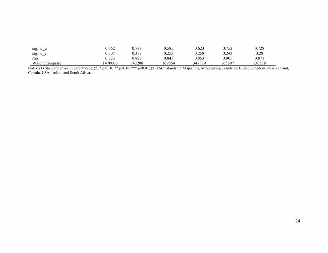
Table 3 Ethnic Capital and Immigrants’ Log Hourly Wage by Country of Origin Group: Full-time Employed Male Immigrants in Australia (Hausman-Taylor Panel Estimation)

Non-English Speaking Countries (NESC) Major English Speaking Countries (ESC)^

General Asia Rest of NESC General UK & Ireland New Zealand Ethnic Capital Network Effect (Weighted log Hourly Wage spatial ethnic network(Wy)) 0.009*** 0.014*** 0.005*** 0.007*** 0.005*** 0.009***

(0.0001) (0.0001) (0.0001) (0.0001) (0.0004) (0.0002) Ethnic Concentration 0.028*** 0.042*** 0.267*** -0.040*** -0.070*** -0.352***

(0.0007) (0.0008) (0.0012) (0.0015) (0.0004) (0.0031) Human Capital Experience 0.035*** 0.039*** 0.014*** 0.042*** 0.027*** 0.055***

(0.0003) (0.0004) (0.0003) (0.0003) (0.0004) (0.0006) Experience -squared -0.001*** -0.001*** 0.0002*** -0.001*** -0.0003*** -0.001***

(5.27e-06) (8.10e-06) (6.77e-06) (5.06e-06) (6.33e-06) (0.00001) Proficiency in English 0.019*** 0.019*** 0.039*** / / /

(0.0018) (0.0021) (0.0037) / / / High Skilled 0.327*** 0.334*** 0.353*** 0.022*** 0.013*** 0.095***

(0.0038) (0.0050) (0.0049) (0.0021) (0.0022) (0.0049) Personal Characteristics Years Since Migration (YSM) 0.039*** 0.021*** 0.036*** 0.067*** 0.063*** 0.053***

(0.0004) (0.0006) (0.0005) (0.0003) (0.0004) (0.0009)YSM-squared -0.0002*** -0.0002*** -0.0002*** -0.001*** -0.001*** -0.001***

(3.79e-06) (6.29e-06) (4.59e-06) (3.23e06) (4.11e-06) (8.10e-06) Married 0.322*** 0.465*** 0.080*** 0.022*** 0.005*** 0.074***

(0.0010) (0.0015) (0.0013) (0.0009) (0.0012) (0.0014) Cohort Effects (5 categories) Yes Yes Yes Yes Yes Yes Year Fixed Effects Yes Yes Yes Yes Yes Yes Observations 1247 638 609 1415 864 381

24

sigma_u 0.662 0.739 0.585 0.623 0.752 0.728 sigma_e 0.307 0.337 0.253 0.258 0.243 0.28 rho 0.823 0.828 0.843 0.853 0.905 0.871 Wald Chi-square 1470000 343208 169854 347379 165897 136578

Notes: (1) Standard errors in parentheses; (2) * p<0.10 ** p<0.05 *** p<0.01; (3) ESC^ stands for Major English Speaking Countries: United Kingdom, New Zealand, Canada, USA, Ireland and South Africa.

25

distance from the host country the effect of ethnic concentration is positive as it can

provide greater opportunities that may overcome competition effects.

In summary, we find the following noteworthy set of results for the effects of

ethnic capital on immigrants’ hourly earnings: (1) The effect of ethnic capital is positive

and strong for both ESC and NESC immigrants, but it does vary across immigrant

groups; (2) The network effect is stronger for immigrants from NESC, especially from

Asia; (3) The ethnic concentration effects are also positive and strong for Asian

immigrants and immigrants from NESC; (4) Once we control for network effects, the

effects of ethnic concentration on immigrants from ESC – a group of countries that have

similar language and cultural backgrounds to Australia – are negative and highly

significant.

In this paper, we find that while immigrant concentration may lower earnings

due to increased competition, as shown in the case of ESC immigrants, when

immigrants have greater cultural and language distance from the host country, they

might “generate” demand for immigrant labor within the cultural/ethnic network and

off-set the initial disadvantages in the host country labor market to some extent.

6.Conclusion

In this paper we have augmented the conventional model of immigrant

earnings, and examined the effect of ethnic capital, particularly spatial ethnic networks

of economic resources on immigrants’ earnings in a panel data setting. We show that

the Hausman and Taylor (1981) model lends itself to addressing endogeneity of the

spatial ethnic network variable, and other related covariates in the augmented

immigrants’ earnings model.

We find that the network variable plays a positive and significant effect on

wage growth in all cases. A stronger social network and linkage helps immigrants to

achieve better economic performance and more successful assimilation. In addition,

wages of immigrants from different cultural and language backgrounds to that of

Australia (e.g. Asia) are more strongly correlated compared to those of other

immigrants.

26

Since the results further confirm that the initial earnings for NESC immigrants,

and for Asian immigrants in particular, are lower than for ESC immigrants, the results

indicate a potentially important role of the ethnic/social network on the economic

integration processes of immigrants from NESC, especially from Asia.

We find that immigrants with a different cultural and language background to

Australia benefit from concentration and networking in a specific region in Australia.

In addition, our study shows that when we control for ethnic network effects and ethnic

concentration, both factors have significant effects for all immigrant groups.

Finally, the results of this study strongly suggest that greater attention to the

role of ethnic capital and immigrant networks on the assimilation process of immigrants

is to be recommended.

27

AppendixA

TableA1:VariableListandDefinitions

     

Human Capital

Potential Experience Age minus the age of graduation. (X1)

Proficiency in English Binary variable, equal to one if proficient in English, based on proficiency

prior to the first year of data. (Z2) High Skilled Binary variable, equal to one if that individual obtained at least a Bachelor

degree or Advanced Certificate. (X2) Personal Characteristics

Years Since Migration (YSM) This variable represents the duration of immigration. (X1)

Married Binary variable, equal to one if that individual is married. (X2)

Arrived 2001-2008 Binary variable, equal to one if that immigrant arrived between 2001 and 2008. (Z1)

Arrived 1991-2000 Binary variable, equal to one if that immigrant arrived between 1991 and 2000. (Z1)

Arrived 1981-1990 Binary variable, equal to one if that immigrant arrived between 1981 and 1990. (Z1)

Arrived 1971-1980 Binary variable, equal to one if that immigrant arrived between 1971 and 1980. (Z1)

Arrived Before 1971 This is a dummy variable, equal to one if that immigrant arrived before 1971. (Z1)

Ethnic Capital

Network Effect (Wy) The weighted (average) logarithm of hourly wage of an individual's ethnic spatial network. (X2)

Ethnic Concentration

The natural logarithm of the proportion of the population of a specific ethnic group to the total population size in a specific region (lagged measures from the previous five-year census). (X1)

Notes: (1) The classification of each variable into one of time varying or invariant, and endogenous or not is indicated in parentheses after the descriptions above. (For example, (X1) indicates that the variable is time varying and exogenous; (X2) indicates that the variable is time varying and endogenous; and (Z1) indicates that the variable is time invariant and exogenous; See also Appendix B.). Tests of endogeneity are provided in Appendix C; (2) Variables treated as endogenous are: Network Effect (Wy), High Skilled, Proficiency in English, and Married.

AppendixB

SpecificationandidentificationoftheHausman‐Taylormodelwitha

spatiallagcomponent

Consider first a model which is essentially the same as that of Hausman and

Taylor (1981):

yit = xitˈβ + ziˈγ + εit

28

where i = 1,…,N (“individuals”) and t = 1,…,T (“time periods”), and xitˈ and ziˈ

are 1 × k and 1 × g vectors of observations respectively on two sets of regressors,

the first of which are time varying and the second are not, as indicated by the

presence/absence of t subscripts; β and γ are the corresponding coefficient vectors.

The disturbances εit, likewise consist of time varying and time invariant components:

εit = αi + ηit

where ηit are independent and identically distributed with E[ηit] = 0, var[ηit] = ση2

and are jointly independent of all xjs, zj and αs for at all i, j, s, t. The time-invariant

components αi are, as in Hausman and Taylor (1981), independently distributed across

individuals, with variance σα2. This last assumption is important for the extension we

consider below.

The regressors are partitioned as xitˈ = [x1itˈ: x2itˈ], where the two sub-vectors

of xitˈ here are k1 × 1, k2 × 1, and ziˈ = [z1iˈ: z2iˈ], with sub-vectors of order g1 × 1,

g2 × 1 respectively. (β and γ are partitioned conformably as βˈ = [β1 : β2ˈ], γˈ = [γ1ˈ

: γ2ˈ]. The point of this partitioning is that x1jt, and z1j are assumed to be jointly

independent of αi, and so, in particular

E[εit | x1it, z1i ] = E[αi | xit, zi] = 0,

which is important for the potential estimability of the entire coefficient vector (βˈ : γˈ);

but this conditional expectation property does not hold for x2it and z2i, and

E[εit | x2it, z2i] = E[αi | x2it, z2i] ≠ 0.

It is convenient in the present case to stack the model by collecting observations

on individuals for each time period (rather than over time by individuals as Hausman

and Taylor do) and write

yt = Xtβ + Zγ + εt

where yt, εt are N × 1 vectors, and Xt, and Z are N × k and N × g respectively,

εt = α + ηt (N × 1 vectors);

here α is the N × 1 vector of time-invariant disturbances (unobserved individual

specific effects) and Xt = [X1t : X2t], Z = [Z1 : Z2], with β and γ partitioned as above.

Note for each t, the elements of ε are mutually uncorrelated and have the same

variance, since the elements of both α and ηt have this structure; although α is

replicated over time periods.

29

In the standard H-T set up the time-invariant property of α provides instruments

which are sufficient for estimation of β, but the time invariant property of Z means

that γ is not estimable on the basis of these alone. If other instruments are available –

in the form of X1t – these, combined with the time invariance of α, can be sufficient for

IV estimation of β and γ.

To see this stacked again across time periods to get

y = Xβ + (ιN ⊗ Z)γ + ε

Here, ε = (ιN ⊗ α) + η and ⊗ denotes Kronecker product. So ιN ⊗ α is N replicates of

α, one on top of another and η is the NT × 1 vector consisting of the T N × 1 vectors

ηt one on top of another. Similarly, X is the Xt’s stacked one on top of another: Xˈ =

[X1ˈ … XTˈ] and X = [X1 : X2], while ι ⊗ Z is N replicates of Z stacked one on top

of another, and ιN ⊗ Z = ιN ⊗ [Z1 : Z2].

Next, let Q be the NT × NT matrix defined by

Q = INT - ιNιNˈ⊗ IT/N

so that for the stacked model Q annihilates Z in the sense that QZ = 0 and also

annihilates the time invariant component, ι ⊗ α of ε, i.e, Q(ιN ⊗ α) = 0.

The matrix of observations on the set of potential instrumental variables is [Q: X1: Z1],

and the necessary order condition obtained by Hausman and Taylor (1981, Proposition

3.2, p. 1385) for the identification of both β and γ is

k1 ≥ g2.

Now consider an extension of this model to accommodate “spatial lags” in the

dependent variable (but without spatial autocorrelation in the disturbances as

considered in, for example, Baltagi (2013, p. 325) and Baltagi and Liu (2011).

The model for each t is now

yt = ρ Wtyt + Xtβ + Zγ + εt, t = 1,…,T

where Xt, Z, and εt = α + ηt as before, and where Wt are T known N × N matrices

of weights (each with zeros on the main diagonal); these may or may not be the same

for all t; ρ is an unknown coefficient, to be estimated alongside β and γ.

Next, note that on the right-hand side of the model

30

Wtyt = ρ Wt[Xtβ + Zγ] + Wtεt

and observe that any given element of Wtεt is independent of the corresponding

element of εt, because of the zero diagonal elements of Wt and the mutual

independence, for each t, of the N elements of the vector εt.

It remains to deal with potential correlation between corresponding elements of

WtXt and εt and also between corresponding elements of WtZ and εt. Because each

diagonal element of Wt is zero, such correlations would have to take the form of

dependencies across individuals, and assuming this away may be reasonable; and if so,

then Wtyt can be absorbed into X1t (or conceivably into Z1 under sufficient time

invariance); and if not, then into X2t (or conceivably into Z2).

The implication of this is that the Hausman-Taylor order condition for the

identification/estimability of ρ, β, γ in the most pessimistic case is strengthened to

k1 ≥ g2 + 1

(where k1 is the number of time varying exogenous variables, and g2 is the number of

the time-invariant endogenous variables) since the presence of Wtyt effectively

increases g2 by one, and for the most optimistic case the condition is weakened to

k1 + 1 ≥ g2

since the presence of Wtyt effectively increases k1 by one. Conceivably the condition

undergoes no change: this is so when it has the effect of increasing k2, arguably the

most likely scenario, or g1.

It is possible therefore to proceed simply by incorporating Wyt into X1t, X2t or

conceivably Z1, Z2. Note that time invariance of Wt is not crucial, because Wtyt will

almost certainly be time varying, and so is likely to be allocated to either X1t or into

X2t, rather than to Z1 or Z2. Once this decision has been made, estimation of ρ, β, γ

can proceed exactly as in Hausman-Taylor (1981). For the model we estimate (see

Appendix A for details), we have k = 6, k1 = 3, g = 6, g2 = 1, so the condition is satisfied,

even in the most pessimistic case. The classification of each of the variables we use

appears in parentheses in Appendix A after the variable descriptions.

The stacked form of the model takes the form

y = ρ diag[Wt]y + Xβ + (ιN ⊗ Z)γ + ε

31

where, diag[Wt] is a NT × NT block diagonal matrix with T diagonal blocks, the tth

being Wt; the other terms are as before. Note that the reduced form of the full model is

y = [I - ρ diag[Wt]]-1Xβ + [I - ρ diag[Wt]]-1(ιN ⊗ Z)γ + [I - ρ diag[Wt]]-1ε

assuming that [I - ρ diag[Wt]] is invertible. The question of the identification of ρ,

β, γ within this reduced form can then be approached along the lines of Bramouille et

al. (2009). Identification fails if (ρo, βo, γo) and (ρ*, β*, γ*) are observationally

equivalent, and this is easily seen to happen if and only if

[I - ρo diag[Wt]](Xβ* + (ιN ⊗ Z)γ*) = [I - ρ*diag[Wt]]](Xβo + (ιN ⊗ Z)γo)

which implies that the columns of [I - λ diag[Wt]](X : (ιN ⊗ Z)) and

diag[Wt](X : (ιN ⊗ Z)) are linearly dependent, where λ is a scalar (which here is equal

to ρ* - ρo). Given that (X : (ιN ⊗ Z)) has full column rank – a minimal identifiability

requirement even in the absence of the spatial autocorrelation feature – this implies (but

is not implied by) singularity of [I – (λ + 1)diag[Wt]], which is evidently problematical

given the assumed invertibility of [I - ρ diag[Wt]]. Therefore, lack of identification in

this setting is not a cause for concern.

32

APPENDIX C

AuxiliaryEstimations

As noted earlier, while our interest lies in our results which address

endogeneity in Table 2 in the paper, below we provide results based on simple panel

data analysis in Table C1 in this Appendix, purely for comparison purposes. The results

below, nevertheless, also provided auxiliary tests for goodness of fit and endogeneity.

The spatial models (models (2) and (4) in Table C1 also show a better data fit13

than do the traditional models (models (1) and (3)). In addition to the higher adjusted

R-square for spatial models (2) and (4) compared to the traditional models (1) and (3),

we have also compared Akaike’s Information Criterion (AIC) results14 to investigate

whether or not this gain is sufficient to overcome the penalty of the loss of the degree

of freedom as reported in Table C1. In these analyses, spatial models in every case

generate a lower AIC, which indicates the spatial models provide a better data fit and

the spatial model is the preferred method to model immigrants’ earnings.

In addition, a comparison of the results in Table 2 based on the Hausman-Taylor

(HT) estimator with the simple panel estimations in Table C1 indicates that some effects

of endogenous variables (language proficiency and skills) are potentially overestimated;

and some effects of exogenous variables are underestimated in the results from pooled

OLS estimations. Furthermore, the pooled OLS model suggests a much stronger initial

earnings disadvantage for immigrants (coefficient of -0.549 in H-T compared to -0.199

in OLS). However, as noted in the paper, the H-T results confirm a significant and

strong effect of YSM across the four specifications, with the coefficients of YSM

around 0.05. It is noteworthy that this result is consistent with Beenstock et al.’s (2010)

13 In a recent study we have examined immigrants’ self-employment decision by a spatial approach. We find that consistent with our results in this paper the spatial model consistently provides a better data fit in the case of analyzing the binary self-employment outcome for immigrants (Wang and Maani, 2014). 14 The AIC, or Akaike Information Criterion, provides a way of measuring a statistical model, in terms

of its relative quality, for a specific collection of data. Consequently it enables the selection of models. It does not allow for the testing of a model, in terms of investigating a hypothesis. However, it is appropriate when the elements of usefulness/appropriateness versus complexity are taken into

consideration. The , where is the likelihood of the model k, and P is the

number of parameters in the model. Adjemian et al. (2010) adopt this approach to select the best model for an individual’s choice of automobile, when considering conventional and spatial models.

33

panel analysis, providing further evidence that panel models reveal a much stronger

effect of assimilation than do OLS models. Among the explanations of the YSM effect

is that the length of time immigrants have been in the host country is likely to affect

their search for sufficient information about the local labor market and their

development of social networks.

The HT estimations suggest a stronger correlation in immigrants’ hourly wage

(coefficient of 0.008) than the panel OLS does (0.007). Compared to a weak significant

positive effect of ethnic concentration on immigrants’ hourly earnings under panel OLS

estimations, under the HT estimations this effect becomes highly significant and larger

(0.027).

In addition, in estimating cohort effects all HT models returned results

confirming a significant improvement in the quality of immigrants than was suggested

from the Panel OLS results.

Moreover, following the method of Ruiz et al. (2010), the Breusch-Pagan test

(Breusch and Pagan, 1980) was applied on the OLS residuals. The results show that the

variance of individual effect α is not zero. In addition, from the HT estimations of ρ we

can see that the unobservable individual error term is around 80% of the total error

variance, supporting our concern that the OLS estimator is not efficient.

34

Table C1: Panel Data Estimates of Log Hourly Wage (No control for endogeneity) Full-time Employed Male Australian-born and Immigrants

Full Sample Immigrant-Only

(1) (2) (3) (4) Ethnic Capital Network Effect (Weighted log Hourly Wage of spatial ethnic network (Wy))

/ / 0.009*** / 0.007***

(0.0024) (0.0026) Ethnic Concentration / / / 0.023*** 0.015* (0.0070) (0.0077) Human Capital Experience 0.021*** 0.010* 0.011* 0.011* 0.011*

(0.0025) (0.0057) (0.0057) (0.0057) (0.0057) Experience -squared -0.0004*** -0.0001 -0.0001 0.9999 0.9999

(0.0001) (0.0001) (0.0001) (0.0001) (0.0001)

Proficiency in English 0.333*** 0.352*** 0.342*** 0.366*** 0.353*** (0.0503) (0.0558) (0.0558) (0.0559) (0.0561)

High Skilled 0.301*** 0.290*** 0.292*** 0.299*** 0.297*** (0.0085) (0.0187) (0.0187) (0.0189) (0.0189)

Personal Characteristics Years Since Migration (YSM)

0.009* 0.004 0.003 0.002 0.002

(0.0045) (0.0054) (0.0054) (0.0054) (0.0055) YSM-squared -0.0001 -0.0001 -0.0001 -0.00004 -0.00004

(0.0001) (0.0001) (0.00009) (0.00009) (0.0001) Married 0.135*** 0.097*** 0.091*** 0.098*** 0.094***

(0.0095) (0.0223) (0.0223) (0.0223) (0.0223) Immigrant -0.199** / / / /

(0.0930) Arrived 2001-2008 0.248*** 0.141 0.151 0.120 0.134

(0.0957) (0.1158) (0.1155) (0.1157) (0.1158) Arrived 1991-2000 0.095 0.003 0.003 0.006 0.005

(0.0699) (0.0860) (0.0858) (0.0858) (0.086) Arrived 1981-1990 0.060 -0.003 0.003 0.005 0.007

(0.0532) (0.0627) (0.0627) (0.0627) (0.0627) Arrived 1971-1980 0.144*** 0.121*** 0.130*** 0.130*** 0.134***

(0.0394) (0.0438) (0.0438) (0.0438) (0.0438) Arrival Before 1971 Reference Group Year Fixed Effects Yes Yes Yes Yes Yes Observations 12782 2662 2662 2662 2662 Adjusted R-square 0.1303 0.1357 0.1398 0.1389 0.1407 AIC 1.269 1.311 1.308 1.309 1.307 Breusch-Pagan Test (Chi-square)

16331 3036 3018 352 355

Notes: (1) HILDA (2001-2008); (2) Standard errors in parentheses; (3) * p<0.10 ** p<0.05 *** p<0.01.

35

Acknowledgements

We wish to thank George Borjas, Daniel Hamermesh, Jacques Poot, Deborah Cobb-Clark, and Jeff Borland, and the participants at the Fourth SOLE|EALE World Meetings (2015) for helpful information or comments. This paper uses unit-record panel data from the Household, Income and Labour Dynamics in Australia (HILDA) Survey. The HILDA Project was initiated and is funded by the Australian Government Department of Families, Housing, Community Services and Indigenous Affairs (FaHCSIA) and is managed by the Melbourne Institute of Applied Economic and Social Research (MIAESR). The findings and views reported in this paper, however, are those of the authors and should not be attributed to any of the persons or organizations acknowledged above.

References

Adjemian, M.K., Lin, C.-Y. C, Williams, J., 2010. Estimating spatial interdependence in automobile type choice with survey data. Transportation Research Part A: Policy and Practice 44, 661-675.

Aguilera, M.B., 2009. Ethnic enclaves and the earnings of self-employed Latinos. Small Business Economics 33, 413-425.

Australian Bureau of Statistics. 2006. 2001 Census tables.

Australian Bureau of Statistics. 2007. 2006 Census tables.

Baltagi, B.H., 2013. Econometric analysis of panel data. Wiley, Chichester, U.K.

Baltagi, B.H., Egger, P.H., Kesina, M. 2013. Firm-level Productivity Spillovers in China's Chemical Industry: A Spatial Hausman-Taylor Approach. Center for Policy Research, Syracuse University, Syracuse.

Baltagi, B.H., Liu, L., 2011. Instrumental variable estimation of a spatial autoregressive panel data model with random effects, Economics Letters 111, 135-137.

Battu, H., Seaman, P., Zenou, Y., 2011. Job contact networks and the ethnic minorities. Labour Economics, 18, 48-56.

Beenstock, M., Chiswick, B.R., Paltiel, A., 2010. Testing the immigrant assimilation hypothesis with longitudinal data. Review of Economics of the Household. 8, 7-27.

Bertrand, M., Luttmer, E.F.P., Mullainathan, S., 2000. Network effects and welfare cultures. The Quarterly Journal of Economics 115, 1019-1055.

Bonacich, P., 1972. Factoring and weighting approaches to status scores and clique identification. Journal of Mathematical Sociology 2, 113-120.

36

Borjas, G.J., 1982. The earnings of male Hispanic immigrants. Industrial and Labor Relations Review 37, 222-239.

Borjas, G.J., 1985. Assimilation, changes in cohort quality, and the earnings of immigrants. Journal of Labor Economics 3, 463-489.

Borjas, G.J., 1987. Self-selection and the earnings of immigrants. The American Economic Review 77,531-553.

Borjas, G.J., 1992. Ethnic capital and intergenerational mobility. The Quarterly Journal of Economics 107, 123-150.

Borjas, G.J., 1995. Assimilation and changes in cohort quality revisited: What happened to immigrant earnings in the 1980s? Journal of Labor Economics 13, 201-245.

Bramouille., Y., Djebbari, H., Fortin, B., 2009. Identification of peer effects through social networks. Journal of Econometrics 150, 41-55.

Breusch, T., Pagan, A., 1980. The Lagrange multiplier test and its applications to model specification in econometrics. Review of Economic Studies 47, 239-253.

Card, D., 1999. The causal effect of education on earnings. In: Ashenfelter, O., Card, D. (Ed.), Handbook of labor economics. Elsevier, Amsterdam.

Card, D., 2000. Estimating the returns to schooling: Progress on some persistent econometric problems. NBER Working Paper 7769. National Bureau of Economic Research.

Chiswick, B.R., 1978. The effect of Americanization on the earnings of foreign-born men. The Journal of Political Economy 86, 897-921.

Chiswick, B.R., 1980. An analysis of the economic progress and impact of immigrants. The Employment and Training Administration, U.S. Department of Labor.

Chiswick, B.R., Lee, Y.L., Miller, P.W., 2005. Immigrant earnings: A longitudinal analysis. Review of Income and Wealth 51, 485-503.

Chiswick, B.R., Miller, P.W., 1995. The endogeneity between language and earnings: International analyses. Journal of Labor Economics 13, 246-288.

Chiswick, B.R., Miller, P.W., 1996. Ethnic networks and language proficiency among immigrants. Journal of Population Economics 9, 19-35.

Chiswick, B.R., Miller, P.W., 1999. Language skill and earnings among legalized aliens. Journal of Population Economics 12, 63-89.

Chiswick, B.R., Miller, P.W., 2002. Immigrant earnings: Language skills, linguistic concentrations and the business cycle. Journal of Population Economics 15, 31-57.

37

Chiswick, B.R., Miller, P.W., 2008. The "Negative" assimilation of immigrants: A special case. IZA Discussion Papers No. 3563. Institute for the Study of Labor (IZA).

Clark, K., Drinkwater, S., 2000. Enclaves, neighbourhood effects and employment outcomes: Ethnic minorities in England and Wales. Journal of Population Economics 15,5-29.

Constant, A., Massey, D.S., 2003. Self-selection, earnings, and out-migration: A longitudinal study of immigrants to Germany. Journal of Population Economics 16, 631-653.

Damm, A., 2009. Determinants of recent immigrants’ location choices: Quasi-experimental evidence. Journal of Population Economics 22, 145-174.

Dustmann, C., Fabbri, F., 2003. Language proficiency and labour market performance of immigrants in the UK. The Economic Journal 113, 695-717.

Edin, P.A., Fredriksson, P., Aslund, O., 2003. Ethnic enclaves and the economic success of immigrants – Evidence from a natural experiment. Quarterly Journal of Economics 118, 329-357.

Fertig, M., Schurer, S., 2007. Earnings assimilation of immigrants in Germany: The importance of heterogeneity and attrition bias. The German Socio-Economic Panel (SOEP) Paper No. 30. German Institute for Economic Research.

Frijters, P., Shields, M.A., Price, S.W., 2005. Job search methods and their success: A comparison of immigrants and natives in the UK. The Economic Journal 115, 359-376.

García, I., Molina, J.A., Navarro, M., 2008. The effects of education on spouses' satisfaction in Europe. Applied Economics 42, 3607-3618.

Gladden, T., Taber, C., 2002. Wage progression among less skilled workers. In: Card, D.E., Blank, R.M. (Ed.), Finding jobs: Work and welfare reform. Russell Sage, New York, 166.

Goetzke, F., 2008. Network effects in public transport use: Evidence from a specially autoregressive mode choice model for New York. Urban Studies 45(2), 407-417.

Goetzke, F., Weinberger, R. 2012. Separating contextual from endogenous effects in automobile ownership models. Environment and Planning A 44, 1032-1046.

Hausman, J.A., Taylor, W.E., 1981. Panel data and unobservable individual effects. Econometrica 49, 1377–1398.

Katz, L., 1953. A new status index derived from sociometric analysis. Psychometrika 18, 39-43.

38

LaLonde, R., Topel, R., 1991. Immigrants in the American labor market: Quality, assimilation, and distribution effects. American Economic Review 81, 297-302.

Lazear, E.P., 1999. Culture and language. Journal of Political Economics 107, 95-126.

Lee, L.F. 2007. Identification and estimation of econometric models with group interactions, contextual factors and fixed-effects. Journal of Econometrics 140 (2), 333-374

LeSage, J., Pace, R.K. 2009. Introduction to spatial econometrics (Statistics: A Series of Textbooks and Monographs) Chapman & Hall/CRC.

Maani, S.A., 2004. Why have Maori relative income levels deteriorated over time? Economic Record 80, 100-123.

Manski, C. 1993. Identification of endogenous social effects: The reflection problem. Review of Economic Studies 60(3), 531-542.

McDonald, J.T., Worswick, C., 1999. The earnings of immigrant men in Australia: Assimilation, cohort effects, and macroeconomic conditions. Economic Record 75, 49-62.

McManus, W., Gould, W., Welch, F., 1983. Earnings of Hispanic men: The role of English language proficiency. Journal of Labor Economics 1, 101-103.

Portes, A., 1987. The social origins of the Cuban enclave economy of Miami. Sociological Perspectives 30, 340-372.

Ruiz, A.C., Gomez, L.N., Narvaez, M.R., 2010. Endogenous wage determinants and returns to education in Spain. International Journal of Manpower 31, 410-425.

Schultz, T.P., 1997. Demand for children in low income countries. In: Rosenzweig, M.R., Stark, O. (Ed.), Handbook of population and family economics, 1 ed. Elsevier B.V., Amsterdam, 367.

Toussaint-Comeau, M., 2008. Do ethnic enclaves and networks promote immigrant self-employment? Economic Perspectives 32, 30-50.

Wang, X., Maani, S.A, 2014. Ethnic capital and self-employment: A spatially autoregressive network approach, IZA Journal of Migration 3:18, 1-24.

Warman, C., 2007. Ethnic enclaves and immigrant earnings growth (Enclaves ethniques et croissance des gains des immigrants). The Canadian Journal of Economics / Revue canadienne d'Economique 40, 401-422.

Yuengert, A.M. (1995) Testing hypotheses of immigrant self-employment. Journal of Human Resources 30(1): 194-204.