Self-Employment and Earnings among High-Skilled Immigrants ...
43
CCIS The Center for Comparative Immigration Studies University of California, San Diego Self-Employment and Earnings among High-Skilled Immigrants in the United States By Magnus Lofstrom Institute for the Study of Labor, Bonn Working Paper 13 July 2000
Transcript of Self-Employment and Earnings among High-Skilled Immigrants ...
CCISThe Center for Comparative Immigration Studies University of California, San Diego
Self-Employment and Earnings among High-Skilled Immigrants in the United States
By Magnus Lofstrom
Institute for the Study of Labor, Bonn
Working Paper 13 July 2000
2
Self-Employment and Earnings among High-SkilledImmigrants in the United States
Magnus Lofstrom
Abstract
This paper uses data from the 1980 and 1990 U.S. Censuses to analyze the labor marketexperience of high-skilled immigrants relative to high-skilled natives. Immigrants arefound to be more likely to be working in one of the high-skilled occupations than natives,but the gap between the two groups decreased in the 1980’s. Given the high self-employment rates of this group of workers, about 20 percent, it is important to study thisaspect of the labor market experience. High-skilled natives are more likely to be self-employed than high-skilled immigrants. Models of the self-employment decision,controlling for differences in socio-economic background, occupation, regionaldifferences in immigrant population proportions, national origin and ethnicity, areestimated. Evidence of positive enclave effects on self-employment probabilities isfound. Predicted earnings of self-employed immigrants are higher throughout most oftheir work life relative to wage/salary immigrants and natives, as well as compared toself-employed natives. Furthermore, there appears to be very little difference in predictedearnings across national origin group of self-employed immigrants. The low variation inpredicted earnings across country of origin groups is not found for wage/salaryimmigrants.
_____I am grateful to Jörgen Hansen, Mark Regets and participants at The Center for Comparative ImmigrationStudies conference on "The International Migration of the Highly Skilled" in San Diego and the annualmeeting of the European Society for Population Economics in Bonn for helpful comments.
1
1. Introduction
The current policy debate about immigration in the U.S. focuses almost entirely on
high-skilled workers. The debate regarding an increase in the number of temporary visas
given to high-skilled workers, particularly in the information technology sector is not
unique to the U.S. In Germany, for example, the government just recently approved
Chancellor Gerhard Schroeder’s “green card” plan. The law gives 20,000 high-skilled
immigrants 5 year temporary work permits in order to ease the perceived shortage of IT
workers. Similar proposals of making temporary work permits more easily available for
high-skilled immigrants are taking place in Great Britain, Ireland and even Sri Lanka.
Although the H-1B visa debate concerns only “temporary” immigration, the
European experience, in particular the German guest worker program, shows that
immigrants who are given temporary work permits are very likely to stay permanently
(Dustmann, 1996). This means that we need to have an understanding of how these, so
called “temporary”, immigrants affect the economy in the long-run. One crucial
determinant of this is the success, or lack thereof, of immigrants in the U.S. labor market.
That is, how do high-skilled immigrants perform in the U.S. labor market relative to high-
skilled natives? No previous study in the economics of immigration literature has
analyzed this issue for this group of immigrants. Instead, an implicit assumption has been
made that highly educated immigrants are relatively successful, as compared to natives,
in the labor market. Furthermore, about one in five high-skilled males are self-employed
in the U.S. This is true for both natives and immigrants. Therefore, to get an accurate
picture of labor market performance of high-skilled immigrants it is necessary to both
include the self-employed and to analyze the decision to become self-employed.

2
This paper looks closely at the labor market performance of the group of immigrants
currently in the U.S. who are most likely to resemble the inflow of immigrants under the
H-1B visa, i.e. high-skilled immigrants. To obtain an accurate prediction of this group’s
performance in the labor market it is necessary to use a large representative sample
containing detailed individual background information on variables such as education,
occupation, geographic location, age, time of arrival in the U.S. and earnings. The only
currently available data set that satisfies these criteria for this minority group of
immigrants, i.e. high-skilled immigrants, is the U.S. Census.
The paper uses data from the 1980 and 1990 U.S. Censuses to show what occupations
the high-skilled immigrants work in, their self-employment rates and differences in the
proportion of high-skilled immigrants by national origin group. I also model the self-
employment decision taking into account differences in socio-economic background,
occupation, regional differences in immigrant population proportions, national origin and
ethnicity. The data shows that immigrants are more likely to be working in one of the
high-skilled occupations than natives, but that the gap between the two groups decreased
in the 1980’s. It also shows that high-skilled natives are more likely to be self-employed
than immigrants. Self-employment rates for high-skilled immigrants appear to vary less
between national origin groups than they do among immigrants overall. Higher
proportions of co-nationals or co-ethnics in an area, so called enclaves, seem to increase
the probability a highly skilled individual selects self-employment. The estimates from
the self-employment decision model are used to control for self-selection into self-
employment and wage/salary work in the estimated earnings functions.
3
The estimated earnings functions are used to generate sector specific measures of
labor market assimilation. I find that both self-employed and wage/salary immigrants are
likely to reach earnings parity with natives, although the result vary somewhat between
immigrant country of origin. However, earnings of self-employed immigrants appear to
be higher throughout most of their work life when compared to the earnings of both
wage/salary and self-employed natives. Furthermore, there appears to be very little
difference in predicted earnings across national origin group of self-employed
immigrants. For example, self-employed Mexican high-skilled immigrants, although a
small group of Mexican immigrants, are predicted to do as well in the U.S. labor market
as European self-employed immigrants. The low variation in predicted earnings across
country of origin groups is not found for wage/salary immigrants.
The paper is organized in the following way. Section 2 describes the data used.
Section 3 outlines and compares traits of immigrants and natives in the two sectors. In
Section 4, the self-employment decision model is described and Section 5 shows the
empirical results. Earnings equations are presented in Section 6. Age-earnings profiles
are also derived and discussed in this section. Finally, Section 7 concludes and
summarizes the results of the study.
2. Data
The data used in this paper are drawn from the 1980 5% A Sample and the 1990 5%
Sample of the U.S. Census of Population. The study includes males between the ages of
22 and 64 who are not residing in group quarters, who are not in military service or
enrolled in school, and who reported working in the year prior to the census. Given the

4
extremely large data set this leaves us with, I extracted a 20 percent randomly selected
sub-sample of native born Americans from the 5% Sample, but kept all immigrants.
Since the 1990 Census is not a random sample of the population, sampling weights were
used. These were set to the appropriate constants for the 1980 Censuses. All weights
were then adjusted accordingly since not all observations for natives were used.
The above described sample includes 1,320,091 observations. From this sample a
sub-sample consisting only of individuals in high-skilled occupations was created. The
occupations were chosen based on the propensity of individuals in the occupation to be
highly educated, where highly educated is defined to be at least a college graduate. The
high-skilled occupations were then grouped into 8 groups. The high-skilled occupational
groups are Management and Finance, Architecture, Engineering, Computer Sciences,
Mathematical and Natural Sciences, Health and Medicine, Social Sciences and Law. The
average number of years of schooling for this sub-sample was 16.65 years in 1980 and
16.7 years in 1990. The number of observation in high-skilled occupations is 106,908.
The earnings regressions in this paper use as the dependent variable log of weekly
total earnings, where weekly earnings is defined to be the sum of earnings from
wage/salary work and self-employment divided by reported weeks worked. This restricts
the sample to include only males who reported positive earnings in the year prior to the
census. Since the self-employed may report negative earnings and would hence be
excluded from the wage regressions, I also estimated the earnings function using weekly
earnings as the dependent variable. The general results that are reported in this paper also
hold for this measure of earnings. It should also be noted that earnings and income

5
reported in the census refers to year prior to the census, i.e. 1979 and 1989 in this paper.
Earnings and income has been realized to 1989 dollars by using the CPI.
It is interesting to note that the selection process that determines who migrates or not,
and hence the labor market performance of immigrants, is believed to be determined by
the relative conditions in host and source country (see for example Borjas, 1987).
However, the majority of studies on immigrant performance have been done based on
ethnic groups, and not on country of origin. In this paper I try to create 10 relatively
homogenous groups based on countries’ geographic location and cultural and economic
conditions, while maintaining a large enough sample size for each group.
It should be noted that any attempt to create homogenous groups will be scarred by
compromises. It is quite clear that there are substantial differences in characteristics such
as self-employment rates and educational attainment between immigrant groups,
Lofstrom (1999). If the group is defined too widely, the impact of variations in these
variables may not be accurately estimated. If the group is too narrowly defined, by
country for example, the sample size will be small for some of the countries. This is
particularly true when studying the sub-group of high-skilled immigrants. However, if
different ethnic groups face different labor market constraints, such as discrimination,
creating groups based on national origin may not be the best way to compose groups.
The national origin groups used in this paper are Mexico, Central/South America,
South East Asia, North East Asia, India/Pakistan, Europe/Canada/Australia/New Zealand,
Africa, Caribbean, Cuba and lastly all other countries of origin. Table A1 in the appendix
describes the countries represented in each national group used in this paper. Although
immigrants are a heterogeneous group, Lofstrom (1999) shows that the national origin
6
groups defined here are quite homogenous within, at least in terms of educational
attainment and ethnicity, and appear to be reasonably defined groups.
3. Descriptive Statistics of High-Skilled Natives and Immigrants
The proportion and the distribution of workers in high-skilled occupations among
natives and immigrants changed in the 1980’s. Table 1 shows that the proportion of male
natives in high-skilled occupations increased from 7.3 percent in 1980 to 8.5 percent in
1990. Although the proportion of workers in high-skilled occupations is higher for
immigrants than natives in both census years, there appears to be a downward trend
among immigrants. In 1980, 9.7 percent of immigrants worked in one of the high-skilled
occupations. This figure dropped by half a percentage points in the 1980’s to 9.2 percent
in 1990. Table 1 also shows that more of the high-skilled individuals are working in
Management and Finance (1.5 and 2.5 percentage point increase from 1980 to 1990 for
natives and immigrants respectively) and in Law (0.7 and 0.2 percentage points) in 1990
than in 1980. The most dramatic increase was, not surprisingly, in the Computer Sciences
where the proportion of high-skilled immigrants more than doubled (an increase from 4.1
percent to 9.1 percent). The proportion of high-skilled natives in this occupation category
also increased, but not as dramatically as for immigrants (from 5.6 percent to 8.6
percent).
Self-employment rates among high-skilled natives and immigrants are substantially
higher than overall self-employment rates, as can be seen in Table 2. Approximately one
fifth of all individuals in high-skilled occupations are self-employed. Not surprisingly,
self-employment rates vary considerably across occupational groups. Nevertheless, it

7
appears that self-employment rates do not differ very much between immigrants and
natives within occupational groups. Also, the overall self-employment rates are quite
similar for immigrants and natives. However, high-skilled natives are more likely to be
self-employed than high-skilled immigrants. Table 2 also shows that the observed
increase in overall self-employment rates for both immigrants and natives is due to an
increase in the self-employment rates of the relatively less-skilled individuals.
Previous studies of immigrant labor market performance have found that skill levels
vary across immigrants from different country of origin, as do self-employment rates (see
for example Borjas, 1994 and Fairlie and Meyer, 1996). Table 3 indicates that skill levels
vary substantially across national origin groups. For example, only about 1 percent of
Mexican immigrants reported in 1990 as working in one of the high-skilled occupations
while in the same year nearly one-third of immigrants from India and Pakistan were high-
skilled. Although there is large variation in the proportions of high-skilled workers
between countries of origin, there is substantially less variation in self-employment rates
of the high-skilled across national origin groups. If we exclude Cubans, of whom 30
percent of the high-skilled are self-employed, self-employment rates vary from 13.7
percent for high-skilled African immigrants to 20.6 percent for the Central/South
American and Middle Eastern national origin groups.
Immigrants in the U.S. have been found to be less successful in the labor market than
natives in the 1980’s (Borjas, 1995 and Betts and Lofstrom 2000). Notably, the self-
employed are excluded from these studies. Lofstrom (1999) however includes the self-
employed in his study and finds that self-employed immigrants do better in the labor
8
market than wage/salary immigrants and are also likely to reach earnings parity with self-
employed natives.
The relative success of self-employed immigrants, compared to natives and
wage/salary immigrants, also appears to hold for the high-skilled self-employed
immigrants, as can be seen in Table 4. High-skilled self-employed natives reported 12
percent lower annual income than their self-employed immigrant counterpart in 1989.
Wage/salary natives in high-skill occupations reported an income disadvantage of 2
percent in 1989, relative to wage/salary immigrants. Furthermore, self-employed
immigrants in less-skilled occupations also reported similar, or slightly higher, income
levels to those of natives in 1989. Wage/salary immigrants in the relatively less-skilled
occupations earned 22 percent less than natives in the same occupations.
Wage/salary and self-employed immigrants in both high-skill and less-skilled
occupations displayed lower relative income, compared to natives, in 1989 than they did
in 1979. It appears that the decline in immigrant labor market performance relative to
natives is not unique to the less-skilled immigrants. However, as can be seen in table 4,
the relative income decline of high-skill immigrants in the 1980’s did not take place in all
occupation groups. For example, immigrant computer scientists reported improvements
in relative income in the 1980’s.
The next two section of this paper will outline a model of the self-employment
decisions and report the results from estimating the model using the above described data.
Mean characteristics for the dependent and independent variables are shown in Table 5.
9
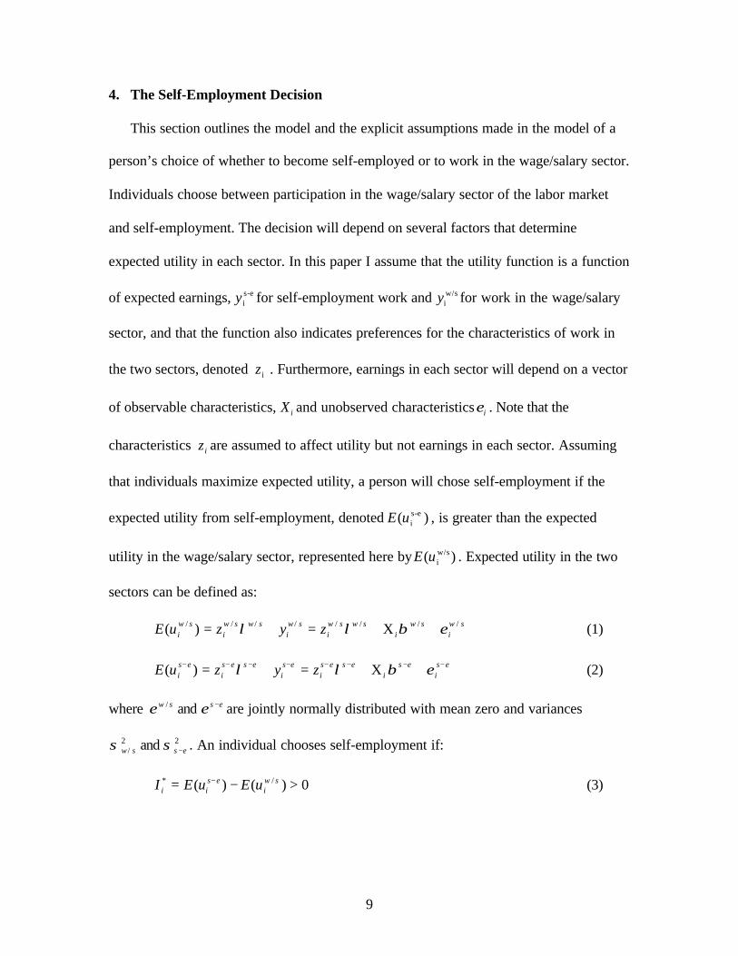
4. The Self-Employment Decision
This section outlines the model and the explicit assumptions made in the model of a
person’s choice of whether to become self-employed or to work in the wage/salary sector.
Individuals choose between participation in the wage/salary sector of the labor market
and self-employment. The decision will depend on several factors that determine
expected utility in each sector. In this paper I assume that the utility function is a function
of expected earnings, e-siy for self-employment work and w/s
iy for work in the wage/salary
sector, and that the function also indicates preferences for the characteristics of work in
the two sectors, denoted iz . Furthermore, earnings in each sector will depend on a vector
of observable characteristics, iX and unobserved characteristics iε . Note that the
characteristics iz are assumed to affect utility but not earnings in each sector. Assuming
that individuals maximize expected utility, a person will chose self-employment if the
expected utility from self-employment, denoted )( e-siuE , is greater than the expected
utility in the wage/salary sector, represented here by )( w/siuE . Expected utility in the two
sectors can be defined as:
swi
swi
swswi
swi
swswi
swi zyzuE //////// )( εβλλ +Χ+=+= (1)
esi
esi
esesi
esi
esesi
esi zyzuE −−−−−−−− +Χ+=+= εβλλ)( (2)
where essw −εε and / are jointly normally distributed with mean zero and variances
22/ and essw −σσ . An individual chooses self-employment if:
0)()( /* >−= − swi
esii uEuEI (3)
10
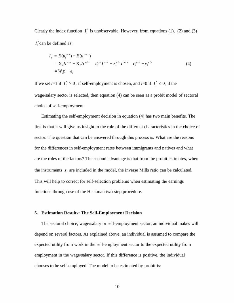
Clearly the index function *iI is unobservable. However, from equations (1), (2) and (3)
*iI can be defined as:
ii
swi
esi
swswi
esesi
swi
esi
swi
esii
eW
zz
uEuEI
+=
−+−+Χ−Χ=
−=−−−−
−
π
εελλββ
)()(////
/*
(4)
If we set I=1 if 0* >iI , if self-employment is chosen, and I=0 if 0* ≤iI , if the
wage/salary sector is selected, then equation (4) can be seen as a probit model of sectoral
choice of self-employment.
Estimating the self-employment decision in equation (4) has two main benefits. The
first is that it will give us insight to the role of the different characteristics in the choice of
sector. The question that can be answered through this process is: What are the reasons
for the differences in self-employment rates between immigrants and natives and what
are the roles of the factors? The second advantage is that from the probit estimates, when
the instruments iz are included in the model, the inverse Mills ratio can be calculated.
This will help to correct for self-selection problems when estimating the earnings
functions through use of the Heckman two-step procedure.
5. Estimation Results: The Self-Employment Decision
The sectoral choice, wage/salary or self-employment sector, an individual makes will
depend on several factors. As explained above, an individual is assumed to compare the
expected utility from work in the self-employment sector to the expected utility from
employment in the wage/salary sector. If this difference is positive, the individual
chooses to be self-employed. The model to be estimated by probit is:

11
eWI ii += π* , where e ∼ N(0,1)
The probability an individual chooses self-employment is:
)(]1Prob[ πWI i Φ== , where Φ(⋅) is the standard normal cumulative density
function. The probability a person chooses the wage/salary sector is then simply:
)(1]0Prob[ πWI i Φ−==
The choice of sector will likely depend on socio-economic characteristics such as age,
education, marital status, disability, and geographic location. If there are differences in
the impact any of these variables have on earnings, we would expect these variables to
affect the self-employment decision. Factors that may affect the expected utility of an
individual, but not an individual’s earnings directly, will also influence the self-
employment decision and need to be controlled for. The estimated marginal effects for
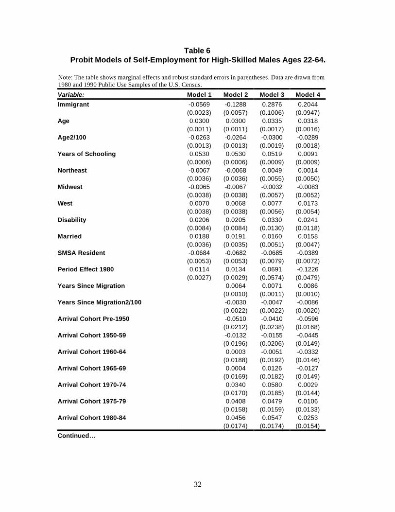
different variations of the above described model are presented in Table 6. The marginal
effects are calculated based on the sample means for continuous variables and for a
discrete change of indicator variables from 0 to 1.
High-skilled natives are on average about 2 percent more likely to be self-employed
than high-skilled immigrants, as shown in Table 5. To test whether this difference is due
to observable socio-economic characteristics, a model including the above discussed
traits, a period effect dummy variable for 1980 and an indicator variable for immigrants
was estimated. The results are presented as Model 1 in Table 6. The estimated difference
between immigrants and natives increases to 5.7 percent when these observable
characteristics are taken into account. Given the estimated results that age and education
affect the self-employment probability positively and the observation that immigrants in

12
these occupations are on average older and more educated, it is not surprising that the
difference between the two groups increase.
It is quite clear that there are other variables that are not included in Model 1 that will
have an effect on an individual’s self-employment decision. For example, for immigrants
it is likely that the number of years in the U.S. and the time of arrival in the U.S will also
influence this decision. Pooling data from the two census years allows for identification
of the effect of both years since migration and arrival cohort. In other words, we can
estimate differences in self-employment probabilities across cohorts controlling for years
spent in the U.S. Model 2 in Table 6 shows the results when these factors are included in
the model. Interestingly, it appears that immigrants who arrived in the 1970’s and early
1980’s are the most likely high-skilled immigrants to select self-employment, holding all
other traits constant. Furthermore, as expected, time spent in the U.S. has a positive effect
on the probability of choosing self-employment.
The models discussed so far are quite restrictive in the sense that they do not allow
for different effects of the observable characteristics on the self-employment decision for
immigrants and natives. Furthermore, one of the reasons for estimating the probits of the
self-employment decision is to derive a selection correction term for choosing self-
employment, i.e. to calculate the inverse Mills ratio. The objective in doing so is to
reduce the possible selection bias that may arise in the estimated earnings models. The
goal is to include in the probit model variables that will influence the self-employment
decision, but that will not affect earnings, i.e. some characteristics iz from the self-
employment decision model above. It is highly desirable, but not necessary, for the probit
model to include instruments that help to predict self-employment but which do not

13
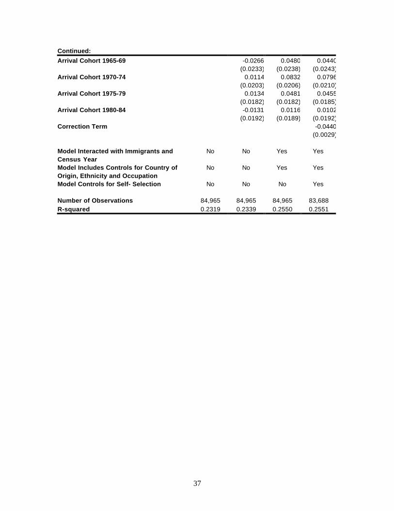
belong directly in the earnings function. Models 3 and 4 in Table 6 include the
instruments used in this paper and also allow for different marginal effects of the
observables for immigrants and natives. In addition, these models control for any changes
in the estimated parameters over the decade studied by interacting all variables with the
1980 period effect. Controls for country of origin group and ethnicity are also
incorporated. Model 4 adds indicator variables for occupations. The role and the
estimated results of the instruments tried in this paper are discussed next.
The first instrument used is a variable to test whether immigrants living in areas
where relatively many co-nationals reside, so called enclaves, may be the reason we
observe higher self-employment rates for some immigrant groups. The sociology
literature commonly speaks of ethnic resources as a determinant in an individual’s choice
of whether or not to choose self-employment (see for example Light, 1984 and Aldrich
and Waldinger, 1990). Examples of ethnic resources are skills or knowledge to provide
services or goods to other co-ethnics or co-nationals, availability of low wage labor,
social support networks that assist an individual in obtaining necessary start-up capital or
in transferring managerial skills. Aldrich and Waldinger (1990) describe “opportunity
structures” as market conditions that may favor goods or services oriented towards co-
ethnics or co-nationals. Immigrants who are living in areas with relatively high
proportions of co-nationals may have a comparative advantage in providing certain goods
or services, food or restaurant services for example, to their co-nationals compared to
natives or other immigrants. The result, according to this theory, is higher self-
employment rates among immigrants living in enclaves. To allow for the possibility that

14
native co-ethnics may also have an advantage similar to that of immigrant co-nationals, a
native ethnic enclave variable is also included in the analysis.
The enclave variables are added to Models 3 and 4 in Table 6. The immigrant enclave
variable represents the proportion of immigrants in the census year of the total population
by SMSA and country of origin. This is calculated by adding up the number of male
immigrants in the sample from a particular country in the SMSA and then dividing this
by the total male population in the sample in the SMSA. For immigrants living in a non-
SMSA area, the proportion is calculated based on the state’s non-SMSA immigrant
population. Given the definition above, it follows that the value of this variable is zero for
all natives. The enclave variable for natives is calculated in the same fashion, but using
the 5 ethnic groups whites, blacks, Asians, Hispanics and others. The variable is set to
zero for all immigrants.
The estimated coefficients of the enclave variables are positive and significant. This
indicates that immigrants living in an area where a greater proportion of co-nationals are
living, increases the probability of self-employment. Model 4 shows that although the
effect is significantly positive for natives as well, it is only about one third of the effect
for immigrants. The results suggest that on average, an increase in the proportion of co-
nationals in the SMSA where the immigrant resides increases the probability of choosing
self-employment by about 0.1 percent. The effect for natives from an increase in the
proportion of co-ethnics is about 0.03 percent. It appears that both immigrants and
natives are positively influenced by an inflow of respective co-nationals and co-ethnics.

15
These results suggest that previously found positive enclave effects also hold for
high-skilled individuals. That is, it is not only small shops and restaurants that are created
by the inflow of immigrants, but also high-skilled firms.
It is also possible that individuals are affected by their co-nationals’ and co-ethnics’
success as entrepreneurs in deciding whether or not to become self-employed. To control
for this possibility two instruments measuring the ratio of self-employment earnings to
wage/salary earnings are included. The first variable is calculated by dividing the average
native self-employment earnings in the SMSA in a given census year by the average
native wage/salary earnings in the same SMSA, by natives’ ethnicity. The second
variable measures the same ratio, but for immigrants by SMSA and national origin group.
The latter variable is set to zero for all natives and the former is set to zero for all
immigrants. It is expected that higher self-employment earnings to wage/salary earnings
ratios are associated with higher self-employment rates, given a set of individual
characteristics, since it essentially measures the relative success of the self-employed in
the area1. The signs of both of the estimated coefficients are positive, as expected, and
significant. However, the impact of a change in the earnings ratio on the probability of
self-employment appears to be stronger for natives than immigrants.
Light (1984) argues that differences in traditions of commerce among immigrants
from different countries help explain differences in self-employment rates among
immigrants in the U.S. This may be one of the reasons for variations in self-employment
rates over countries of origin that is not captured by the observable traits in the model.
1 One concern with incorporating these variables into the self-employment decision models is that they maybe determined endogenously and consequently lead to inconsistent estimators. However, given that theratios are relative group characteristics by SMSA and not individual characteristics, this seems somewhat
16
Also, if immigrants experience discrimination in the labor market and if discrimination
varies over source countries, this also needs to be controlled for in the model. To attempt
to incorporate these country specific unobservables, dummy variables for the national
origin groups are included in Models 3 and 4. The estimated coefficients on the national
origin group variables, not shown in tables in order to keep the length of the tables
reasonably short, indicate that there is virtually no difference in the probability an
individual selects self-employment across national origin groups, holding all observable
characteristics constant. The exception is that high-skilled immigrants from South East
Asia are slightly less likely to choose to become entrepreneurs compared to statistically
similar immigrants from the Middle East. Furthermore, there is no statistical difference in
the self-employment probability of high-skilled whites, blacks, Asian and Hispanics.
These results should not be interpreted as that there are no differences in self-
employment propensities between immigrants from different countries or across
individuals of different ethnicity. It means that once we condition our sample on being
highly skilled, there are small differences across these groups. Several earlier studies have
shown, using population representative samples, that both self-employment rates and
earnings vary across national origin groups (e.g. Camarota, 2000, Fairlie and Meyer,
1996, Lofstrom, 1999 and Yuengert, 1995). It is however very interesting to note that
there is very little variation across high-skilled immigrant and ethnic groups.
As mentioned above, one of the advantages of estimating a model of the self-
employment decision model is that the estimates can be used to control for self-selection
in the earnings models. The consistent estimates obtained from the earnings models can
unlikely. The earnings ratio is not clearly endogenous, but may simply reflect entrepreneurial conditions oropportunities in an area.

17
then be used to derive age-earnings profiles. From these profiles, we can answer the
question if immigrants’ earnings are likely to converge with the earnings of natives’ over
the work-life. The specification in Model 4 is used for the two-step Heckman selection
correction models estimated and described below.
6. Estimation Results: Labor Market Assimilation
Immigrants’ earnings in the wage/salary sector have been found to not converge with
natives' earnings (Borjas, 1985 and 1995) over the work life. Earnings of immigrants start
out at a lower point and rise more rapidly over time than natives’ earnings. However,
parity is not reached. The labor market performance of self-employed immigrants, who
are excluded from Borjas’ studies, have been found to be significantly different from
wage/salary immigrants. Lofstrom (1999) finds that earnings of self-employed
immigrants is predicted to converge with native wage/salary earnings at around age 30
and native self-employed earnings at around age 40. This section will look at the labor
market success of high-skilled immigrants in both the wage/salary and self-employment
sector.
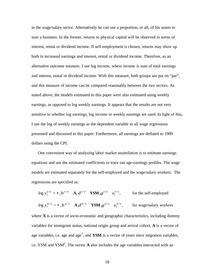
The earnings models estimated in this paper use as the dependent variable log of
weekly earnings. To try to take into account the possibility that self-employed workers
earn a return on physical capital, I also estimate models using as the dependent variable
the log of weekly income, which includes any earnings from wage/salary work and/or
self-employment earnings and in addition, any interest, rental or dividend income. If an
individual is deciding between a wage/salary job or self-employment, he can keep his
assets in, for example, savings accounts, the stock market, bonds, or real estate and work
18
in the wage/salary sector. Alternatively he can use a proportion, or all, of his assets to
start a business. In the former, returns to physical capital will be observed in terms of
interest, rental or dividend income. If self-employment is chosen, returns may show up
both in increased earnings and interest, rental or dividend income. Therefore, as an
alternative outcome measure, I use log income, where income is sum of total earnings
and interest, rental or dividend income. With this measure, both groups are put on “par”,
and this measure of income can be compared reasonably between the two sectors. As
stated above, the models estimated in this paper were also estimated using weekly
earnings, as opposed to log weekly earnings. It appears that the results are not very
sensitive to whether log earnings, log income or weekly earnings are used. In light of this,
I use the log of weekly earnings as the dependent variable in all wage regressions
presented and discussed in this paper. Furthermore, all earnings are deflated to 1989
dollars using the CPI.
One convenient way of analyzing labor market assimilation is to estimate earnings
equations and use the estimated coefficients to trace out age-earnings profiles. The wage
models are estimated separately for the self-employed and the wage/salary workers. The
regressions are specified as:
esi
esi
esi
esi
esi uy −−−−− +++= γδβ YSMA×log , for the self-employed
swi
swi
swi
swi
swi uy /////log +++= γδβ YSMA× , for wage/salary workers
where X is a vector of socio-economic and geographic characteristics, including dummy
variables for immigrant status, national origin group and arrival cohort, A is a vector of
age variables, i.e. age and age2, and YSM is a vector of years since migration variables,
i.e. YSM and YSM2. The vector A also includes the age variables interacted with an

19
immigrant dummy variable. The years since migration variable is equal to zero for all
natives.
The models described above were estimated both by ordinary least squares with no
selection correction and also by heteroskedastic robust ordinary least squares using the
inverse Mills ratio to correct for selection bias. The estimated coefficients from the
earnings models are presented in Tables 7 and 8 where Models 1, 2 and 3 are the
equations without selectivity correction and Model 4 includes the correction term
calculated based on estimation of Model 4 in Table 6.
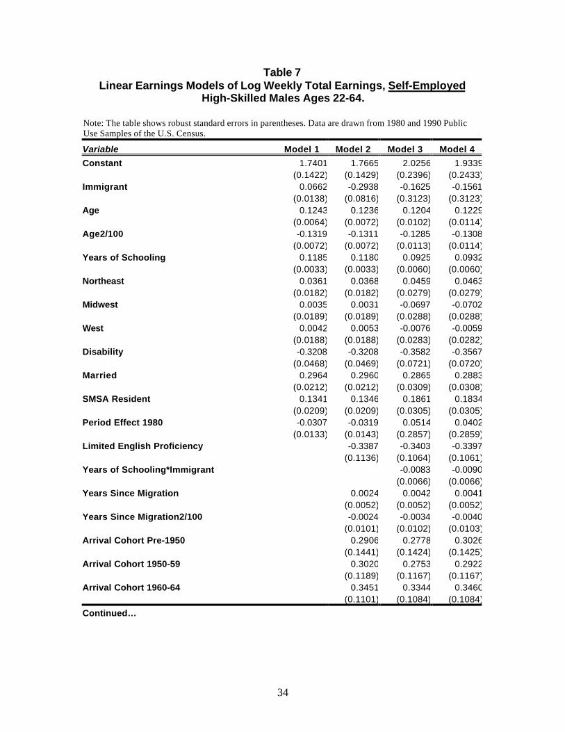
Self-employed immigrants report higher weekly earnings than natives even when age
and education are controlled for, as shown in Model 1 of Table 7. However, the estimated
coefficient, 0.07, of the immigrant dummy shows that differences in observable
characteristics explain about two thirds of the earnings advantage of self-employed
immigrants (the observed difference between the two groups is about 21 percent). Model
2 in the same table shows that only the most recent immigrants in 1989 earned less than
natives. It also appears that there is no significant difference in weekly earnings across all
other arrival cohorts, holding years since migration constant. The higher observed
earnings of wage/salary immigrants, compared to natives, can be explained by the
variables included in Model 1 of Table 8. In fact, the observed immigrant earnings
advantage of about 5 percent turns into an earnings gap favoring natives by
approximately 7 percent. The results in Model 2 indicate that the estimated initial
earnings upon arrival in the U.S. do not differ between arrival cohorts.
The last two models in Tables 7 and 8 are more flexible than Models 1 and 2 in the
sense that they allow for differences in the effect of the included variables for immigrants

20
and natives. In addition, they also include controls for national origin groups and
occupation. The last model, Model 4, adds a control for self-selection. The results do not
appear to be very sensitive to the inclusion of selection correction term. The discussion
will therefore focus on the results for Model 4 shown in Tables 7 and 8.
Immigrants have been found to earn lower returns to schooling than natives (Betts
and Lofstrom, 2000). The estimated coefficient on the variable interacting years of
schooling with the immigrant indicator variable allows us to test if this also holds for
high-skilled immigrants. The estimated coefficients on this variable is negative but
statistically insignificant for both self-employed and wage/salary workers. It appears that
high-skilled immigrants earn similar returns to education as natives do.
The sign of the coefficient on the inverse Mills ratio variable tells us whether there is
an overall positive or negative selection into each sector. Not surprisingly, the correction
term indicates that there is positive selection into both wage/salary work and self-
employment. That is, individuals who choose self-employment are better suited for self-
employment, at least in terms of earnings, than are the persons who choose to work in the
wage/salary sector and vice versa. However, the coefficient on the correction term for the
self-employed is not statistically significant from zero.
The estimated coefficients and correction terms from the earnings equations, Model 4
in tables 7 and 8, can be used to predict earnings individuals who chose self-employment
would have earned if they instead had chosen wage/salary work, and vice versa. This can
be done by applying the estimated coefficients from the wage/salary model, for example,
to each self-employed individual’s observed characteristics and estimated correction
term. Predicted average earnings can then be calculated separately for immigrants and
21
natives. The exercise gives us insight to “the returns to self-employment”. Given that
there appears to be positive selection into the wage/salary sector, we expect predicted
wage/salary earnings for the self-employed, calculated according to the above described
method, to be lower than the predicted self-employment earnings. Indeed, this is what is
found. However, the predicted wage/salary earnings do not decrease equally for self-
employed immigrants and natives. The predicted drop for natives is around 11 percent
while the decline for immigrants is more than twice that, approximately 25 percent. This
indicates that high-skilled immigrants earn higher returns to self-employment than
natives. This is somewhat surprising given that we observe lower self-employment rates
for high-skilled immigrants than natives. If immigrants earn greater returns to self-
employment than natives, we would expect that they also would be more likely to select
self-employment than natives.
One possible explanation for this finding is that there may be constraints, for example
capital constraints, that are more binding for immigrant than natives and that this prevent
some high-skilled immigrants from becoming entrepreneurs. A finding that is consistent
with this conjecture is that the predicted self-employment earnings for wage/salary
workers are higher than the predicted wage/salary earnings for immigrants, by 6 percent,
and lower for natives, by 6 percent. On average, high-skilled wage/salary immigrants
would earn more if they had chosen self-employment.
To address the issue of the rate at which high-skilled immigrants assimilate into the
U.S. labor market, and if they are likely to reach earnings parity with high-skilled natives,
we want to compare predicted earnings over the work life for immigrants and natives. A
convenient way to analyze immigrant labor market assimilation is to compare predicted

22
age-earnings profiles for natives and immigrants. Figures 1,2 and 3 show the predicted
age-earnings profiles derived from Model 4 in Tables 7 and 8. It traces out the average
predicted log weekly earnings over age by using the estimated coefficients. The notes in
the figures show what assumptions are made and which reference groups are used.
Figure 1 shows that high-skilled self-employed immigrants are likely to have higher
earnings than statistically similar natives throughout their work life. Wage/salary
immigrants are expected to have lower earnings than natives at young ages, but are
predicted to reach earnings parity with natives in the wage/salary sector at around age 50.
It is quite possible that the relative labor market performance varies across country of
origin groups. To address this possibility, I derived separate age-earnings profiles for 4
large country of origin groups. Figures 2 and 3 show the predicted earnings for natives
and these national origin groups, North East Asia, Mexico, India/Pakistan and
Europe/Canada/Australia/New Zealand.
The figures indicate that the variation in earnings across country of origin is less
among self-employed immigrants. The results also suggest that within a country of origin
group, there are differences in the relative success in the labor market. For example, high-
skilled self-employed immigrants from Mexico show higher lifetime earnings than their
self-employed native counterpart. Mexican immigrants who are working in the
wage/salary sector are not predicted to even reach earnings parity with wage/salary
natives. It is also well worthwhile to point out that there appears to be no significant
difference in the predicted earnings between whites, blacks, Hispanics and Asians. The
estimated coefficients in both the wage/salary and the self-employment equations are all
within ±2 standard errors of each other.
23
7. Summary and Conclusions
This paper shows, using data from the 1980 and 1990 U.S. Censuses, that a very high
proportion of high-skilled workers are self-employed. Approximately one fifth of both
high-skilled natives and immigrants are entrepreneurs. The paper also tests for enclave
effects on the self-employment probability. Higher proportion of co-nationals and co-
ethnics are found to increase the probability an individual selects self-employment. The
relative success of co-nationals and co-ethnics in the self-employment sector is also
found to positively affect the self-employment probability.
Immigrants in high-skilled occupations report higher annual earnings than natives.
Self-employed natives in high-skill occupations reported 12 percent lower earnings than
self-employed immigrants in 1989. The earnings advantage for wage/salary immigrants
in that year was about 2 percent. Although both self-employed and wage/salary
immigrants are predicted to at least reach earnings parity with natives over their work
life, self-employed immigrants are predicted to have higher earnings than self-employed
natives throughout most of their work life.
I also find some indications that constraints to enter self-employment, for example
capital constraints, may be more binding for high-skilled immigrants than for high-skilled
natives.
The variation in earnings across country of origin is less among self-employed
immigrants than among wage/salary immigrants. As has been found among the
immigrant population overall, the paper also finds that self-employed high-skilled
immigrants do relatively better, compared to natives, in the U.S. labor market than

24
immigrants working in the wage/salary sector. However, immigrants in both sectors
generally do well in the labor market.
Given the findings in this paper, it seems likely that high-skilled immigrants will
contribute positively to the U.S. economy. This however assumes that immigrants do not
have a negative impact on wages and employment opportunities. Although researchers
studying these potential negative effects of immigration generally find no significant
effects or only small negative effects (see for example Altonji and Card, 1990 and Borjas,
1994), we do not know if this is also the case for the high-skilled workers. Further
research into the possible impact of high-skilled immigration on high-skilled natives’
labor market outcomes appears to be warranted.
25
References
Aldrich, Howard E. and Waldinger, Roger. (1990) “Ethnicity and Entrepreneurship.”Annual Review of Sociology 16:111-35.
Altonji, Joseph G. and Card, David. (1991) “The Effects of Immigration on the LaborMarket Outcomes of Less-Skilled Natives.” In John Abowd and RichardFreeman, eds. Immigration, Trade and the Labor Market, U of Chicago Press.
Betts, Julian R. and Lofstrom, Magnus. (2000) “The Educational Attainment ofImmigrants: Trends and Implications.” in George J. Borjas (ed) Issues in theEconomics of Immigration. University of Chicago Press.
Borjas, George J. (1985) “Assimilation Changes in Cohort Quality and the Earnings ofImmigrants.” Journal of Labor Economics, 4:463-89.
Borjas, George J. (1986) “The Self-Employment Experience of Immigrants.” Journal ofHuman Resources 21:485-506.
Borjas, George J. (1994) “The Economics of Immigration.” Journal of EconomicLiterature 32:1667-717.
Borjas, George J. (1995) “Assimilation Changes in Cohort Quality Revisited: WhatHappened to Immigrant Earnings in the 1980’s?” Journal of Labor Economics2:201-45.
Bregger, John E. (1996) “Measuring Self-employment in the United States.” MonthlyLabor Review 3-9.
Camarota, Steven A. (2000) “Reconsidering Immigrant Entrepreneurship: AnExamination of Self-Employment Among Natives and the Foreign Born.”Washington DC, Center for Immigration Studies.
Carliner, Geoffrey. (1980) “Wages, Earnings and Hours of First, Second, and ThirdGeneration American Males.” Economic Inquiry 1:87-102.
Chiswick, Barry R. (1978) “The Effect of Americanization on the Earnings of Foreign-born Men.” Journal of Political Economy 5:897-921.
Cummings, Scott, (1980) Self-Help in Urban America: Patterns of Minority BusinessEnterprise, Kenikart Press, New York.
Dustmann, C. (1996) “Return Migration: The European Experience” Economic Policy,22, 213-50.
26
Fairlie, Robert W. and Meyer, Bruce D. (1996) “Ethnic and Racial Self-EmploymentDifferences and Possible Explanations.” Journal of Human Resources 31:757-93.
Light, Ivan (1984) Immigrant and Ethnic Enterprise in North America. Ethnic and RacialStudies 7:195-216.
Lofstrom, Magnus (1999) “Labor Market Assimilation and the Self-EmploymentDecision of Immigrant Entrepreneurs.” IZA Discussion Paper No. 54.
Yuengert, Andrew M. (1995) Testing Hypotheses of Immigrant Self-Employment.Journal of Human Resources 30:194-204.

27
Table 1Proportions of Natives and Immigrants in High-Skilled Occupations, Males
Ages 22-64. Data are drawn from1980 and 1990 Public Use Samples of the U.S. Census. (Number of
Observation in High-Skilled Occupations is 106,908).
1980 1990 Change1980-1990
Occupation: Natives Immigrants Natives Immigrants Natives Immigrants
High-Skilled Overall 7.3% 9.7% 8.5% 9.2% 1.2% -0.5%
Distribution of High-Skilled OccupationsManagement and Finance 23.0% 16.2% 24.5% 18.7% 1.5% 2.5%Architecture 2.4% 2.9% 2.4% 3.0% 0.0% 0.1%Engineering 32.5% 37.8% 28.5% 34.8% -4.0% -3.0%Computer Sciences 5.6% 4.1% 8.6% 9.1% 3.0% 5.0%Mathematical and Natural Sciences 6.5% 7.3% 6.0% 6.9% -0.5% -0.4%Health and Medicine 15.8% 25.9% 15.0% 21.7% -0.8% -4.2%Social Sciences 3.4% 2.8% 3.5% 2.6% 0.1% -0.2%Law 10.9% 3.0% 11.6% 3.2% 0.7% 0.2%

28
Table 2Self-Employment Rates by High-Skilled Occupations, Males Ages 22-64.
Data are drawn from 1980 and 1990Public Use Samples of the U.S. Census.
1980 1990 Change1980-1990
Occupation: Natives Immigrants Natives Immigrants Natives Immigrants
All Occupations 12.8% 12.5% 12.9% 13.0% 0.1% 0.5%
Less-Skilled Overall 12.1% 11.9% 12.2% 12.5% 0.1% 0.6%High-Skilled Overall 21.0% 18.6% 20.7% 18.4% -0.3% -0.2%
Management and Finance 14.9% 11.5% 18.3% 17.6% 3.4% 6.1%Architecture 43.6% 32.0% 34.7% 31.3% -8.9% -0.7%Engineering 3.0% 3.0% 3.6% 3.6% 0.6% 0.6%Computer Sciences 3.2% 2.8% 6.2% 5.8% 3.0% 3.0%Mathematical and Natural Sciences 4.5% 3.4% 5.7% 3.7% 1.2% 0.3%Health and Medicine 57.4% 48.4% 50.6% 48.0% -6.8% -0.4%Social Sciences 10.0% 11.2% 19.4% 14.2% 9.4% 3.0%Law 52.3% 49.7% 45.3% 42.5% -7.0% -7.2%

29
Table 3Self-Employment Rates and Proportions of Immigrants in High-Skilled Occupations by National Origin Groups,
Males Ages 22-64. Data are drawn from 1980 and 1990 Public Use Samples of the U.S. Census.
Proportion (and Sample Size) in High Skill Occupations Self-Employment Rates1980 1990 Change 1980 1990 Change
National Origin Group: 1980-1990 1980-1990
Mexico 1.0% (279) 0.9% (492) -0.1% 24.4% 19.5% -4.9%Central/South America 7.0% (779) 5.3% (1,385) -1.7% 19.6% 20.6% 1.0%South East Asia 15.3% (1,357) 12.6% (2,496) -2.7% 20.9% 14.6% -6.3%North East Asia 19.0% (1,941) 16.9% (3,296) -2.1% 13.8% 14.7% 0.9%India, Pakistan 42.9% (1,953) 31.4% (2,921) -11.5% 13.5% 18.9% 5.4%Middle East/Egypt 17.8% (776) 19.0% (1,933) 1.2% 23.1% 20.6% -2.5%Europe,CAN,AUS,NZ 9.6% (5,877) 11.8% (6,201) 2.2% 19.1% 20.0% 0.9%Africa 18.0% (311) 16.5% (673) -1.5% 17.4% 13.7% -3.7%Caribbean 5.1% (389) 4.7% (550) -0.4% 15.7% 16.2% 0.5%Cuba 7.7% (648) 7.5% (763) -0.2% 29.3% 30.4% 1.1%Other 8.3% (801) 5.5% (507) -2.8% 21.3% 15.0% -6.3%

30
Table 4Total Annual Income (in $1989) and Ratio of Average Total Annual Income, Natives/Immigrants, by High-Skilled
Occupations, Males Ages 22-64. Data are drawn from 1980 and 1990 Public Use Samples of the U.S. Census.
1980 1990Wage/Salary Self-Employed Wage/Salary Self-Employed
Natives/ Natives/ Natives/ Natives/Occupation: Natives Immigrants Immigrants Natives Immigrants Immigrants Natives Immigrants Immigrants Natives Immigrants Immigrants
Less-Skilled Overall 29,347 25,997 1.13 31,312 34,733 0.90 29,503 24,270 1.22 32,881 33,378 0.99High-Skilled Overall 43,676 46,478 0.94 73,765 85,858 0.86 49,875 50,747 0.98 84,059 95,838 0.88
Management and Finance 39,063 36,865 1.06 57,835 51,817 1.12 45,045 42,777 1.05 58,602 55,640 1.05Architecture 36,950 37,570 0.98 45,018 44,983 1.00 43,171 41,531 1.04 49,863 53,886 0.93Engineering 44,036 44,227 1.00 55,330 57,120 0.97 45,679 47,042 0.97 52,911 54,257 0.98Computer Sciences 42,089 42,698 0.99 43,677 41,364 1.06 43,531 44,271 0.98 52,730 51,561 1.02Math and Natural Sciences 40,338 43,876 0.92 66,645 74,536 0.89 42,015 42,989 0.98 53,817 55,768 0.97Health and Medicine 54,441 65,135 0.84 87,007 100,471 0.87 74,387 81,457 0.91 106,134 123,225 0.86Social Sciences 43,890 50,779 0.86 57,272 55,838 1.03 45,749 51,531 0.89 67,649 58,297 1.16Law 52,127 53,815 0.97 72,953 63,645 1.15 73,329 64,136 1.14 92,670 85,547 1.08

31
Table 5Mean Characteristics for Natives and Immigrants in High-Skilled
Occupations, Males Ages 22-64. Data are drawn from 1980 and 1990 PublicUse Samples of the U.S. Census.
Natives ImmigrantsVariable:
Self-Employed 0.208 0.185Weeks Worked 49.52 48.90Hours per Week 44.60 44.88Log Weekly Wage 6.74 6.80Age 39.49 40.04Years of Schooling 16.59 17.32Northeast 0.234 0.301Midwest 0.234 0.167West 0.222 0.301Disability 0.034 0.015Married 0.763 0.799SMSA Resident 0.899 0.968Period Effect 1980 0.447 0.389Years Since Migration N/A 17.33Limited English Proficiency N/A 0.021Proportion of Natives of the Same 0.767 N/AEthnicity in SMSARatio of S-E earnings to W/S earnings 0.659 N/Aby SMSA and EthnicityProportion of Immigrants from Same N/A 0.010Country of Origin Group in SMSARatio of S-E earnings to W/S earnings N/A 0.703by SMSA and National Origin Group
Number of Observations 71,888 35,020
32
Table 6Probit Models of Self-Employment for High-Skilled Males Ages 22-64.
Note: The table shows marginal effects and robust standard errors in parentheses. Data are drawn from1980 and 1990 Public Use Samples of the U.S. Census.
Variable: Model 1 Model 2 Model 3 Model 4
Immigrant -0.0569 -0.1288 0.2876 0.2044(0.0023) (0.0057) (0.1006) (0.0947)
Age 0.0300 0.0300 0.0335 0.0318(0.0011) (0.0011) (0.0017) (0.0016)
Age2/100 -0.0263 -0.0264 -0.0300 -0.0289(0.0013) (0.0013) (0.0019) (0.0018)
Years of Schooling 0.0530 0.0530 0.0519 0.0091(0.0006) (0.0006) (0.0009) (0.0009)
Northeast -0.0067 -0.0068 0.0049 0.0014(0.0036) (0.0036) (0.0055) (0.0050)
Midwest -0.0065 -0.0067 -0.0032 -0.0083(0.0038) (0.0038) (0.0057) (0.0052)
West 0.0070 0.0068 0.0077 0.0173(0.0038) (0.0038) (0.0056) (0.0054)
Disability 0.0206 0.0205 0.0330 0.0241(0.0084) (0.0084) (0.0130) (0.0118)
Married 0.0188 0.0191 0.0160 0.0158(0.0036) (0.0035) (0.0051) (0.0047)
SMSA Resident -0.0684 -0.0682 -0.0685 -0.0389(0.0053) (0.0053) (0.0079) (0.0072)
Period Effect 1980 0.0114 0.0134 0.0691 -0.1226(0.0027) (0.0029) (0.0574) (0.0479)
Years Since Migration 0.0064 0.0071 0.0086(0.0010) (0.0011) (0.0010)
Years Since Migration2/100 -0.0030 -0.0047 -0.0086(0.0022) (0.0022) (0.0020)
Arrival Cohort Pre-1950 -0.0510 -0.0410 -0.0596(0.0212) (0.0238) (0.0168)
Arrival Cohort 1950-59 -0.0132 -0.0155 -0.0445(0.0196) (0.0206) (0.0149)
Arrival Cohort 1960-64 0.0003 -0.0051 -0.0332(0.0188) (0.0192) (0.0146)
Arrival Cohort 1965-69 0.0004 0.0126 -0.0127(0.0169) (0.0182) (0.0149)
Arrival Cohort 1970-74 0.0340 0.0580 0.0029(0.0170) (0.0185) (0.0144)
Arrival Cohort 1975-79 0.0408 0.0479 0.0106(0.0158) (0.0159) (0.0133)
Arrival Cohort 1980-84 0.0456 0.0547 0.0253(0.0174) (0.0174) (0.0154)
Continued…

33
Continued:
Limited English Proficiency 0.0915 0.0480(0.0248) (0.0204)
Years of Schooling*Immigrant -0.0109 -0.0049(0.0016) (0.0011)
Proportion of Immigrants from Same 0.1901 0.0926Country of Origin Group in SMSA (0.0690) (0.0507)Proportion of Natives of the Same 0.0206 0.0318Ethnicity in SMSA (0.0123) (0.0113)Ratio of S-E earnings to W/S earnings 0.0329 0.0213by SMSA and National Origin Group (0.0124) (0.0086)Ratio of S-E earnings to W/S earnings 0.0579 0.0412by SMSA and Ethnicity (0.0112) (0.0099)
Model Interacted with Immigrants and No No Yes YesCensus YearModel Includes Controls for Country of No No Yes YesOrigin and EthnicityModel Includes Controls for Occupation No No No Yes
Number of Observations 106,908 106,908 105,545 105,545Log Likelihood -45,364 -45,310 -44,691 -38,357
34
Table 7Linear Earnings Models of Log Weekly Total Earnings, Self-Employed
High-Skilled Males Ages 22-64.
Note: The table shows robust standard errors in parentheses. Data are drawn from 1980 and 1990 PublicUse Samples of the U.S. Census.
Variable Model 1 Model 2 Model 3 Model 4
Constant 1.7401 1.7665 2.0256 1.9339(0.1422) (0.1429) (0.2396) (0.2433)
Immigrant 0.0662 -0.2938 -0.1625 -0.1561(0.0138) (0.0816) (0.3123) (0.3123)
Age 0.1243 0.1236 0.1204 0.1229(0.0064) (0.0072) (0.0102) (0.0114)
Age2/100 -0.1319 -0.1311 -0.1285 -0.1308(0.0072) (0.0072) (0.0113) (0.0114)
Years of Schooling 0.1185 0.1180 0.0925 0.0932(0.0033) (0.0033) (0.0060) (0.0060)
Northeast 0.0361 0.0368 0.0459 0.0463(0.0182) (0.0182) (0.0279) (0.0279)
Midwest 0.0035 0.0031 -0.0697 -0.0702(0.0189) (0.0189) (0.0288) (0.0288)
West 0.0042 0.0053 -0.0076 -0.0059(0.0188) (0.0188) (0.0283) (0.0282)
Disability -0.3208 -0.3208 -0.3582 -0.3567(0.0468) (0.0469) (0.0721) (0.0720)
Married 0.2964 0.2960 0.2865 0.2883(0.0212) (0.0212) (0.0309) (0.0308)
SMSA Resident 0.1341 0.1346 0.1861 0.1834(0.0209) (0.0209) (0.0305) (0.0305)
Period Effect 1980 -0.0307 -0.0319 0.0514 0.0402(0.0133) (0.0143) (0.2857) (0.2859)
Limited English Proficiency -0.3387 -0.3403 -0.3397(0.1136) (0.1064) (0.1061)
Years of Schooling*Immigrant -0.0083 -0.0090(0.0066) (0.0066)
Years Since Migration 0.0024 0.0042 0.0041(0.0052) (0.0052) (0.0052)
Years Since Migration2/100 -0.0024 -0.0034 -0.0040(0.0101) (0.0102) (0.0103)
Arrival Cohort Pre-1950 0.2906 0.2778 0.3026(0.1441) (0.1424) (0.1425)
Arrival Cohort 1950-59 0.3020 0.2753 0.2922(0.1189) (0.1167) (0.1167)
Arrival Cohort 1960-64 0.3451 0.3344 0.3460(0.1101) (0.1084) (0.1084)
Continued…

35
Continued:
Arrival Cohort 1965-69 0.3801 0.3360 0.3480(0.1018) (0.0994) (0.0993)
Arrival Cohort 1970-74 0.3762 0.2995 0.3044(0.0949) (0.0936) (0.0936)
Arrival Cohort 1975-79 0.3644 0.3104 0.3157(0.0903) (0.0880) (0.0880)
Arrival Cohort 1980-84 0.2653 0.2277 0.2328(0.0967) (0.0936) (0.0936)
Correction Term 0.0226(0.0152)
Model Interacted with Immigrants and No No Yes YesCensus YearModel Includes Controls for Country of No No Yes YesOrigin, Ethnicity and OccupationModel Controls for Self- Selection No No No Yes
Number of Observations 21,663 21,663 21,663 21,598R-squared 0.1579 0.1586 0.1797 0.1797

36
Table 8Linear Earnings Models of Log Weekly Total Earnings, Wage/Salary
High-Skilled Males Ages 22-64.
Note: The table shows robust standard errors in parentheses. Data are drawn from 1980 and 1990 PublicUse Samples of the U.S. Census.
Variable Model 1 Model 2 Model 3 Model 4
Constant 3.3657 3.3703 3.0306 3.0457(0.0353) (0.0354) (0.0569) (0.0571)
Immigrant -0.0716 -0.2181 0.0691 0.0890(0.0043) (0.0146) (0.0774) (0.0785)
Age 0.0901 0.0900 0.0930 0.0915(0.0017) (0.0021) (0.0025) (0.0032)
Age2/100 -0.0902 -0.0905 -0.0940 -0.0928(0.0021) (0.0021) (0.0032) (0.0032)
Years of Schooling 0.0660 0.0661 0.0749 0.0745(0.0010) (0.0010) (0.0017) (0.0017)
Northeast 0.0619 0.0617 0.1010 0.1009(0.0055) (0.0055) (0.0082) (0.0083)
Midwest 0.0115 0.0111 -0.0103 -0.0099(0.0057) (0.0057) (0.0086) (0.0086)
West 0.0316 0.0315 0.0413 0.0398(0.0057) (0.0057) (0.0082) (0.0083)
Disability -0.1552 -0.1549 -0.1822 -0.1827(0.0163) (0.0163) (0.0258) (0.0259)
Married 0.1205 0.1214 0.1229 0.1217(0.0052) (0.0052) (0.0075) (0.0075)
SMSA Resident 0.1447 0.1449 0.1606 0.1642(0.0077) (0.0077) (0.0110) (0.0110)
Period Effect 1980 -0.0635 -0.0619 0.4590 0.4622(0.0041) (0.0044) (0.0682) (0.0684)
Limited English Proficiency -0.1613 -0.1521 -0.1592(0.0340) (0.0340) (0.0349)
Years of Schooling*Immigrant -0.0020 -0.0018(0.0021) (0.0021)
Years Since Migration 0.0144 0.0132 0.0132(0.0015) (0.0016) (0.0016)
Years Since Migration2/100 -0.0158 -0.0171 -0.0169(0.0035) (0.0036) (0.0036)
Arrival Cohort Pre-1950 -0.0646 0.0129 0.0051(0.0407) (0.0430) (0.0436)
Arrival Cohort 1950-59 -0.0509 -0.0046 -0.0071(0.0293) (0.0304) (0.0309)
Arrival Cohort 1960-64 -0.0300 0.0535 0.0521(0.0263) (0.0270) (0.0275)
Continued…
37
Continued:
Arrival Cohort 1965-69 -0.0266 0.0480 0.0440(0.0233) (0.0238) (0.0243)
Arrival Cohort 1970-74 0.0114 0.0832 0.0796(0.0203) (0.0206) (0.0210)
Arrival Cohort 1975-79 0.0134 0.0481 0.0455(0.0182) (0.0182) (0.0185)
Arrival Cohort 1980-84 -0.0131 0.0116 0.0102(0.0192) (0.0189) (0.0192)
Correction Term -0.0440(0.0029)
Model Interacted with Immigrants and No No Yes YesCensus YearModel Includes Controls for Country of No No Yes YesOrigin, Ethnicity and OccupationModel Controls for Self- Selection No No No Yes
Number of Observations 84,965 84,965 84,965 83,688R-squared 0.2319 0.2339 0.2550 0.2551

38
Table A1.Definition of National Origin Groups.
Mexico:MexicoSouth and Central America :Argentina, Bolivia, Brazil, Chile, Colombia, Ecuador, Falkland Islands, French Guyana, Guyana,Paraguay, Peru, Suriname, Uruguay, Venezuela, Belize, Costa Rica, El Salvador, Guatemala,Honduras, Nicaragua, Panama.South East Asia:Bangladesh, Brunei, Burma, Cambodia, Indonesia, Laos, Macau, Malaysia, Philippines, Thailand,Vietnam.North East Asia:China, Hong Kong, Japan, North Korea, Singapore, South Korea, Taiwan.India/Pakistan:Bangladesh, Bhutan, India, Nepal, Pakistan, Sri Lanka.Middle East/Egypt:Bahrain, Cyprus, Iran, Iraq, Israel, Jordan, Kuwait, Lebanon, Oman, Qatar, Saudi Arabia, Syria,Turkey, United Arab Emirates, Yemen, Egypt.Europe, Canada, Australia, New Zealand:Albania, Andorra, Austria, Belgium, Bulgaria, Czechoslovakia, Denmark, Faeroe Islands, Finland,France, Germany, Gibraltar, Greece, Hungary, Iceland, Ireland, Italy, Liechtenstein, Luxembourg,Malta, Monaco, Netherlands, Norway, Poland, Portugal, Romania, San Marino, Spain, Sweden,Switzerland, United Kingdom, Vatican, Yugoslavia, Soviet Union, Canada, Australia, NewZealand.Caribbean:Anguilla, Antigua and Barbuda, Aruba, Bahamas, Barbados, British Virgin Islands, CaymanIslands, Dominica, Dominican Republic, Grenada, Guadeloupe, Haiti, Jamaica, Martinique,Montserrat, Netherlands Antilles, St. Barthelemy, St.Kitts-Nevis, St. Lucia, St. Vincent and theGrenadines, Trinidad and Tobago, Turks and Caicos Islands.Cuba:CubaAfrica:Algeria, Angola, Benin, Botswana, British Indian Ocean Territory, Burkina Faso, Burundi,Cameroon, Cape Verde, Central African Republic, Chad, Comoros, Congo, Djibouti, EquatorialGuinea, Ethiopia, Gabon, Gambia, Ghana, Glorioso Islands, Guinea, Guinea-Bissau, Ivory Coast,Juan de Nova Island, Kenya, Lesotho, Liberia, Libya, Madagascar, Malawi, Mali, Mauritania,Mayotte, Morocco, Mozambique, Namibia, Niger, Nigeria, Reunion, Rwanda, Sao Tome andPrincipe, Senegal, Mauritius, Seychelles, Sierra Leone, Somalia, South Africa, St. Helena,Sudan, Swaziland, Tanzania, Togo, Tromelin Island, Tunisia, Uganda, Western Sahara, Zaire,Zambia, Zimbabwe.

39
Figure 1.Predicted Age-Earnings Profile for Self-Employed and Wage/Salary Immigrants and Natives.
Note: The age-earnings profiles are derived from the estimated Models 4 in Tables 7 and 8. Individuals are assumed to be married, have 18 years ofschooling and are residing in a SMSA. Furthermore, the estimates for North East Asian immigrants who arrived between 1975 and 1979 are used.Baseline is 1990.
6.1
6.2
6.3
6.4
6.5
6.6
6.7
6.8
6.9
7
7.1
22 24 26 28 30 32 34 36 38 40 42 44 46 48 50 52 54 56 58 60 62 64
Age
Lo
g W
eekl
y E
arn
ing
s
Wage/Salary Natives Self-Employed Natives Wage/Salary Immigrants Self-Employed Immigrants

40
Figure 2.Predicted Age-Earnings Profile for Self-Employed Immigrants and Natives by Country of Origin group.
Note: The age-earnings profiles are derived from the estimated Model 4 in Table 7. Individuals are assumed to be married, have 18 years of schoolingand are residing in a SMSA. Furthermore, the estimates for who arrived between 1975 and 1979 are used. Baseline is 1990.
6.1
6.2
6.3
6.4
6.5
6.6
6.7
6.8
6.9
7
7.1
2 2 2 4 2 6 2 8 3 0 3 2 3 4 3 6 3 8 4 0 4 2 4 4 4 6 4 8 5 0 5 2 5 4 5 6 5 8 6 0 6 2 6 4
Age
Lo
g W
eekl
y E
arn
ing
s
Natives North East Asia Mexico India and Pakistan Europe, Canada, Austral ia and New Zealand

41
Figure 3.Predicted Age-Earnings Profile for Wage/Salary Immigrants and Natives by Country of Origin group.
Note: The age-earnings profiles are derived from the estimated Model 4 in Table 8. Individuals are assumed to be married, have 18 years of schoolingand are residing in a SMSA. Furthermore, the estimates for who arrived between 1975 and 1979 are used. Baseline is 1990.
6.1
6.2
6.3
6.4
6.5
6.6
6.7
6.8
6.9
7
7.1
22 24 26 28 30 32 34 36 38 40 42 44 46 48 50 52 54 56 58 60 62 64
Age
Log
Wee
kly
Ear
ning
s
Natives North East Asia Mexico India and Pakistan Europe, Canada, Australia and New Zealand