NBER WORKING PAPER SERIES

CRIME, URBAN FLIGHT, AND THECONSEQUENCES FOR CITIES

Julie Berry CullenSteven D. Levitt

Working Paper 5737

NATIONAL BUREAU OF ECONOMIC RESEARCH1050 Massachusetts Avenue

Cambridge, MA 02138September 1996

We would like to thank Daron Acemoglu, Philip Cook, David Cutler, Jonathan Gruber, Jen-yHausman, Lawrence Katz, John Lott, David Mustard, James Poterba, William Wheaton, and seminarparticipants at Harvard, MIT, and the University of Pennsylvania for helpful comments. We aregratefil to Rich Robinson of CIESIN for providing the Census data extracts. Comments can beaddressed either to Julie Berry Cullen, Building E-52, Department of Economics, MassachusettsInstitute of Technology, Cambridge, MA 02142, or to Steven Levitt, Harvard Society of Fellows,78 Mount Auburn Street, Cambridge, MA 02138. e-mail addresses: jberry@mit.edu;slevitt@fm.harvard. edu. The financial support of the National Science Foundation and the NationalInstitute on Aging is gratefully acknowledged. All remaining errors are the sole responsibility ofthe authors. This paper is part of NBER’s research program in Public Economics. Any opinionsexpressed are those of the authors and not those of the National Bureau of Economic Research.

01996 by Julie Berry Cullen and Steven D. Levitt. All rights reserved. Short sections of text, notto exceed two paragraphs, may be quoted without explicit permission provided that full credit,including O notice, is given to the source.

NBER Working Paper 5737September 1996

CRIME, URBAN FLIGHT, AND THECONSEQUENCES FOR CITIES

ABSTRACT

This paper demonstrates that rising crime rates in cities are correlated with city depopulation.

Instrumental variables estimates, using measures of the certainty and severity of a state’s criminal

justice system as instruments for city crime rates, imply that the direction of causality runs from

crime to urban flight. Using annual city-level panel data, our estimates suggest that each additional

reported crime is associated with a one person decline in city residents. There is some evidence that

increases in suburban crime tend to keep people in cities, although the magnitude of this effect is

small. Analysis of individual-level data from the 1980 census confirms the city-level results and

demonstrates that almost all of the crime-related population decline is attributable to increased out-

migration rather than a decrease in new arrivals to a city. Those households that leave the city

because of crime are much more likely to remain within the SMSA than those leaving the city for

other reasons. The migration decisions of high-income households and those with children are much

more responsive to changes in crime than other households. Crime-related mobility imposes costs

on those who choose to remain in the city through declining property values and a shrinking tax

base.

Julie Berry CullenDepartment of Economics, E52Massachusetts Institute of TechnologyCambridge, MA 02142jberry@mit.edu

Steven D. LevittHarvard Society of Fellows78 Mount Auburn StreetCambridge, MA 02138and NBERslevitt@fas.harvard. edu

The difficulties confronting large American cities in recent decades are well

documented.’ The urban riots of the late 1960s turned the post-war suburbanization trend

into large-scale urban flight. A declining tax base, shrinking federal subsidies, tax

limitations, and city residents in need of greater public services has pushed many cities to

the brink of fiscal crisis. Among the greatest difficulties faced by large American cities is

crime. Violent crime rates in U.S. cities with populations over 500,000 in 1993 were four

times higher than in cities with populations below 50,000, and seven times greater than in

rural areas. z Higher crime rates in large cities are even more remarkable when one

considers that both per capita expenditures on police and the level of victim precaution

(e.g. locking doors, private security guards, alarm systems) are much greater in large

cities.3

This paper examines the link between crime and urban flight.4 Although there is an

extensive literature analyzing this subject (e.g. Taeuber and Taeuber 1965, Bradford and

Kelejian 1973, Frey 1979, MarshalI 1979, Marshall and O’Flaherty 1987), there has been

relatively little focus on the role of crime in explaining the phenomenon, A handful of

studies have included the level of crime as a right-hand side variable in cross-city OLS

1 See, for instance, Bradbury, Downs, and Small (1 982), Gottdeiner (1 986), Wilson

(1 987), and Inman, Craig, and Lute (1 994).

2 The Uniform Crime Re~o rts, which reflect only those crimes reported to the police,are likely to understate the actual difference in crime rates across city types because of thegreater likelihood a crime will be reported to the police in smaller cities (Levitt 1995),

3 In 1990-1991, cities with population over one million spent an average of $210 per

capita on police protection, whereas cities with populations below 75,000 residents

expended an average of $97 per capita (U.S. Department of Commerce 1993).

4 While urban flight is interesting in its own right, declines in city population are also

correlated with increases in the percent of families below the poverty line in the city, the

fraction of city residents failing to complete high school, and declines in median housing

values. Thus, urban flight proxies for city decline more generally.

1

estimates of urban flight. These studies typically obtain a positive relationship between

crime rates and urban flight (e.g. Frey 1979, Grubb 1982, Katzman 1980, Sampson and

Wooldredge 1986).5

In contrast to previous research on the topic,

impact of changes in crime rates rather than levels.

our analysis focuses primarily on

There are both theoretical and

the

methodological justifications for examining changes in crime rates. From a theoretical

perspective, the simplest residential choice model predicts that changes in crime rates, not

levels, will influence changes in city populations On a practical level, focusing on changes

mitigates problems associated with non-comparabilities in crime reporting rates, crime

definitions, and police department practices across cities (O’Brien 1985).

Section I documents the strong empirical correlation between rising crime rates and

central city population declines using a panel of 137 cities over the period 1976-1993.

After controlling for other factors, each additional reported crime in a central city is

associated with a net decline of about one resident. Higher suburban crime rates tend to

keep people in central cities, although the magnitude of this effect is much smaller than for

crimes within cities.

Of course, one cannot necessarily draw any causa/ conclusions from these

5 Previous research has also documented a positive relationship between population

turnover and crime rates at the neighborhood level, especially in poor neighborhoods (Smith

and Jarjoura 1988, Taylor and Covington 1988). In contrast to that literature, which

focuses on gross flows of residents, our analysis is concerned with net population changes.

G In a simple model where property values fully capitalize the costs and benefits of a

location, then changes in amenities can be captured by changes in housing values without

any net population change. Relocation costs and heterogeneous tastes affect the

composition of the residents, but do not necessarily imply any change in the total number

of city residents. In this paper, we take the empirical regularity of fluctuating city

populations as a starting point, leaving the theoretical puzzle of why property values do not

fully adjust for future work.

2

estimates. While the most obvious causal link runs from rising crime rates to urban flight,

it is also possible that an omitted third factor may be responsible for both rising crime and

urban flight. For instance, if population loss in shrinking cities is disproportionately

comprised of high income individuals (who tend to have lower rates of crime victimization),

then the average crime rate among remaining city residents will rise, even if each resident’s

risk of victimization is unchanged. On the other hand, since crime rates are strongly

positively correlated with city size, city growth is likely to be correlated with rising crime

rates. If that is the case, OLS may understate the causal impact of crime on city

population.

We attempt to establish a causal link between crime and urban flight through the

use of instrumental variables in Section Il. A valid instrument must affect the crime rate

but not otherwise belong in the equation explaining city population changes. The logical

source of such instruments is changes in the punitiveness of the criminal justice system. In

particular, we use lagged changes in state prison commitments and state prison releases

per crime. These variables are demonstrated to affect crime in the predicted manner, yet

are plausibly excluded from the city population equation. The estimated impact of crime on

city population using 2SLS are slightly larger than the OLS estimates, suggesting that any

bias in the OLS estimates resulting from omitted variables or compositional changes in city

population is overwhelmed by the tendency for large cities to have higher crime rates.

A major limitation of the above panel-data analysis is that it addresses only

aggregate population changes. Using PUMS data from the 5 percent sample of the 1980

census yields a number of additional insights in Section Ill. We are able to obtain estimated

migration in and out of 81 U.S. cities by income category, race, and family status. Using

census data, it is also possible to distinguish between increasing out-migration and

3

declining in-migration and to identify the destinations of those who leave cities. Our results

suggest that almost all of the impact of crime on city population results from increased out-

migration; the link between changes in crime and in-migration appears weak. Seventy

percent of those people leaving central cities due to crime remain within the SMSA,

compared to forty percent of all central city out-migrants. The mobility decisions of high

income households are five times more responsive to changing crime rates than those of

the poor. Whites and blacks show similar responses to crime. Households with children

are twice as responsive to crime as households without children.

Section IV summarizes the results of the paper and provides rough calculations of

the costs of crime and crime-related mobility for cities and their residents. In addition to

the direct costs of victimization, crime imposes numerous other costs on city residents.

Because crime-related out-migration is concentrated among the rich, rising crime will be

accompanied by increasing concentrations of poverty. While those remaining in the city

are likely to have greater need for locally provided public services such as police protection,

public education, public transportation, and city hospitals, the ability to provide those

services is diminished. Evidence also suggests that rising crime rates are associated with

declining housing prices, eroding the property tax base, which is the primary revenue

source of cities, In the presence of fiscal increasing returns (Blanchard and Summers

1987), cities can be caught in a downward spiral in which rising tax rates lower real

wages. To the extent that peer effects are important to human capital development (Case

and Katz 1991, Benabou 1993, Cutler and Glaeser 1995) the exodus of the most mobile

groups will exert a further negative externality on those left behind.

4

Section 1: Correlations between Changes in Crime and C hanaes in Citv POK)UIation

We begin our analysis by specifying a simple reduced-form relationship between

changes in crime and changes in city population. We include changes in both central city

and suburban crime rates in the specification, along with a range of other covariates

described below to capture socioeconomic, economic and demographic characteristics of

the city, SMSA, and state. Our logic for focusing on changes in crime rates is that in

equilibrium, the previous level of crime in a city will already have been incorporated into the

individual’s residential choice decision (although potentially with some adjustment lag).

The theoretical prediction that changes and not levels of crime should effect changes in

city population is strongly supported by the empirical evidence presented later in the paper.

The basic specification we employ is as follows:

Aln (CITY_ POPit) = ~lACITY CRIMEit + fi2ASUBURB_CRIMEit + P3UNEM

+ ~4INC;MEit_l + ~~aln (S TATEPOpit_l) (1)+ B6%BLACKit_1 + AGEit_l G + At + Yr + eit

where the subscripts 1, t, and r index cities, time, and regions respectively. The population

variable is in log changes whereas the two crime variables are in changes in per capita

rates. This specification allows the impact of changes in crime on mobility to be

independent of the level of crime; other specifications such as log changes in both crime

and population, or changes in levels of both variables, lead to similar results when

evaluated at the sample mean. With the exception of the crime variables, which enter

contemporaneously and will be instrumented, one year lags are used for all of the other

covariates to reduce endogeneity problems.’ In addition to economic controls, a set of

7 It is unclear whether these covariates should enter in levels or changes. The same

logic that makes changes rather than levels of crime rates appropriate suggests changes for

5

variables reflecting the age distribution of the population, lagged log-changes in state

populations, and a variety of indicator variables are included to capture other systematic

sources of variation.

Equation (1) is estimated using a

137 U.S. central cities with populations

panel of data covering the years 1976-1993 for

greater than 100,000 in 1975. Throughout the

analysis we allow for heteroskedasticity by city size. Data limitations necessitate a number

of compromises because the analysis is performed at the city level. Annual data on net

migration is unavailable, so changes in overall city population, which are influenced not

only by migration but also by birth, death, and immigration rates, are used instead. Birth

and death rates (approximately 1.5 and 0,9 per hundred) are relatively low compared to

gross flows due to migration (roughly six percent of the U.S. population moves across

county lines each year (Schwartz 1987)). a Immigration rates in the United States over the

time period examined are roughly 0.2 percent per year. Sampson and Wooldredge (1 986),

using data from the decennial census, find that their results are not sensitive to the choice

of overall city population changes versus net migration flows. Our results are also robust

to the use of net migration data from the Census in Section Ill.

The crime rates used are the per capita number of index crimes reported to the

police and collected in Uniform Crime Re~orts. Given that less than half of all

these other variables as well. On the other hand, the demographic controls may be picking

up differential levels of mobility across groups (e.g. young adults move six times as

frequently as those over age 65), which suggests levels as the correct choice. The results

that follow include levels. An earlier version of this paper (available on request from the

authors) utilized changes with little effect on the crime coefficients.

8 Moreoverr movers affect city populations in both the community they leave and the

community they move to, whereas births and deaths affect only one community. This

effectively doubles the importance of migration in explaining city-level population flows.

6

victimizations are reported to the police, the UCR crime data are potentially contaminated

by substantial measurement error. Victimization data, however, is not available below the

level of regions, necessitating the use of UCR statistics. In a previous version of this

paper, we attempted to disaggregate crimes into violent and property, obtaining similar

coefficients on both types. The high degree of collinearity between those two crime

classifications makes it difficult to separately identify the coefficients, particularly in the IV

estimates presented in Section Il. Consequently we present only estimates aggregated

over all crime categories in the tables; full results disaggregating crimes into violent and

property are available from the authors on request. We use crime rates in the rest of the

Metropolitan Statistical Area, excluding the central city, as our measure of suburban crime.

The types of covariates available in a city-level panel are less than ideal. Most city-

Ievel data is collected only in decennial census years, necessitating a tradeoff between the

level of aggregation of the data and the frequency of collection. As a general principle, we

use the most disaggregated annual source of data available in our regressions.

Unemployment rates are available annually by SMSA. Per capita income is available on a

yearly basis at the state level. The age distribution of the population is also available

annually by state. We choose to linearly interpolate the percent of a city’s population that

is black from decennial census data rather than using state-level data. In the OLS

regressions of this section, the primary strategy adopted for minimizing the problems

associated with the lack of good controls is the inclusion of numerous indicator variables:

year dummies, region dummies corresponding to the nine census regions, and city-fixed

effects. Because the left-hand side variable is already in differences, a city-fixed effect

picks up within-city trends over time. In some cases, we replace the year and region

indicators with region-year interactions to better control for regional economic and

7

demographic shifts as well as possible changes over time in tastes for climate or other

regional characteristics. Two further points about the lack of good control variables are

also worth noting, First, in the instrumental variables estimates, as long as the omitted

variables are uncorrelated with the instruments, consistent estimates of the crime

parameters will nonetheless be obtained. Second, in Section Ill of the paper where we use

individual-level data from the census and therefore have a much better set of controls, we

obtain similar results whether we use the limited set of covariates utilized here or a greatly

expanded set of covariates including household-level controls.

Summary statistics for the data are presented in Table 1. For those variables that

enter equation (1 ) as changes, summary statistics for both the levels and changes are

shown. OLS regression results are presented for a range of specifications in Table 2.

Column 1 corresponds directly to equation (1). Column 2 adds city-fixed effects. Column

3 includes both city-fixed effects and region-year interactions. Columns 4-6 mirror the first

three columns with once-lagged crime levels added to the specification.

The coefficients on the crime rate changes are in the top two rows. Including city-

fixed effects and region-year interactions improves the fit of the model but has little effect

on the crime variables. The crime coefficients are statistically significant in all

specifications. For the purposes of interpreting the results, the change in city residents for

each additional reported crime is a useful measure of the magnitude of the effect. It is

straightforward to demonstrate that D1 closely approximates (but slightly overstates) that

measure and thus is directly interpretable. g The interpretation of ~z is more complicated,

9 The larger is the variation in crime rates relative to the variation in city populations,

the closer is the approximation. In our data, the standard deviation of percent changes in

year-to-year crime rates is five to six times larger than the corresponding value for city

populations.

8

however, because it depends on the relative sizes of the city and suburban populations. In

our data, suburbs on average have three times as many residents as central cities. Thus,

to determine the change in city residents per additional suburban crime at the mean of our

sample, one must divide ~z by

is associated with a decline in

three. According

city population of

to the estimates, an

about one resident.

additional city crime

The coefficient on

suburban crime rates translate into an impact about one-sixth as large as that for city crime

rates. A one-standard deviation change in city crime rates (roughly a ten percent change

in crime), translates into a decline in city population of slightly less than one percent.

The other covariates enter in a plausible manner. A percentage point change in

SMSA unemployment leads to a 0.035 to 0.23 percent decline in city population. This

translates into a decrease of between 5 and 35 city residents for each 100 additional

persons unemployed. That estimate is similar in magnitude to the state-level estimates in

Blanchard and Katz (1 992), The size of the unemployment effect on city populations

increases substantially when city-fixed effects are included. There is some evidence that

cities located in states with higher per capita income tend to grow faster. Cities with a

higher initial fraction of black residents appear to grow more slowly, mirroring the earlier

findings of Frey (1 979). There is little within-city variation in percent black, however, so

with city-fixed effects the estimates are imprecise. The age coefficients, which are relative

to the omitted category “over age 65, ” flip sign with the inclusion of city-fixed effects.

The coefficient on lagged state population growth is very large with estimated elasticities

between 0.33 to 0.64. Excluding this variable, however, has little impact on the crime

parameters.

The specifications in columns 1-3 of Table 2 assume that changes in crime and

population occur contemporaneously. To test the possibility of partial adjustment or lagged

9

responses to crime, columns 4-6 include the once-lagged crime rate in levels. None of the

lagged crime rates are statistically significant, and the magnitudes of the coefficients are

generally less than a tenth as large as those associated with changes in crime rates.

Lagged crime changes also appear to have weak explanatory power, as do /cads of crime

changes.

We have also explored numerous other variants of the basic specification (not

shown in tabular form). Estimating the model using fixed effects or longer differences in

place of one-year differences yields similar estimates. Dividing the sample according to

time period, we cannot reject the null of equal coefficients across the two parts of the

sample. Finally, splitting the sample by city size, we cannot reject the null of equality

across cities greater than or less than 250,000 in population.

Sect ion 11:Establishing Causa Iitv in the Relationship between C itv PODulations and Crime

w

The preceding section documents a strong negative correlation between changes in

crime rates and changes in city populations, but cannot provide any clear guidance about

the direction of causality. While one possibility is that rising crime rates lead to urban

flight, there are also a number of plausible channels through which population changes

might affect crime rates. Looking cross-sectionally, crime rates are much higher in large

urban areas, suggesting that increases in city population lead to higher crime rates, due

perhaps to increased criminal opportunities in densely settled areas, the increased

anonymity of big-city life, or because big cities attract likely criminals (e.g. Glaeser and

10

Sacerdote 1996).’0 If that is the case, the estimates of the previous section may

understate the true causal relationship between city crime and depopulation since city

growth will lead to higher crime rates.

On the other hand, there are a number of factors suggesting that the OLS estimates

may overstate the true magnitude of the causal impact of city crime. First, an omitted

third variable that is positively correlated with changes in crime rates and negatively

correlated with city population changes could explain the negative OLS coefficient.

Second, if the pool of residents in shrinking cities is increasingly comprised of less mobile

groups that are also more likely to engage in criminal activity, then depopulation might be

associated with increasing per capita crime rates.’l Wilson (1 987) further argues for non-

Iinearities between concentrations of poverty and crime that would exacerbate this bias.

Third, if there is measurement error in city populations, then a ratio-bias problem is present

since crime rates are defined on a per capita basis. Unlike the standard regression model

where measurement error in the left-hand side variable will not bias the coefficients, when

the dependent variable appears in the denominator of the right-hand side variables,

measurement error induces a negative bias.12 Finally, city population may be an incorrect

10 Where data are available, urban crime rates are almost always higher than rural crime

rates. Beattie (1 995), for instance, reports that for the period 1690-1720, prosecutions for

offenses against property in the city of London were almost seven times greater than the

mostly rural counties of Essex and Sussex, An apparent exception to this pattern is

American cities in the late 1800s; the emergence of the professional police force in the

latter half of the 19th century appears to have dramatically reduced the amount of disorderin large American cities (Monkkonen 1981).

11 One caveat to this argument is that the rich are more likely to report crimes to the

police than the poor, so even if the actual victimization rate rises due to compositional

changes, the reported crime rate may not.

12 When an individual household’s mobility decision is used as the dependent variable in

Table 8, ratio bias is not a concern. The results are unaffected, suggesting ratio-bias is not

11

denominator for crime rates if a large fraction of the victims of crime are commuters or

tourists, If many former city residents relocate to the suburbs but continue to work in the

central city and be victimized therer13 this could induce a spurious negative correlation

between city populations and city crime rates as measured in this paper.

We attempt to determine causality through the use of instrumental variables. In

what follows, we focus our efforts on instrumenting for city crime rates, treating suburban

crime rates as exogenous to city population. From a theoretical perspective, the

endogeneity stories discussed above are more directly applicable and compellin9 for city

crime rates (e.g. reverse causality and ratio bias). Empirically, we have also experimented

with instrumenting for both city and suburban crime rates, with no impact on the city crime

coefficients. Because of a weaker first-stage fit, we can never reject that the suburban

crime coefficients are equal to zero when instrumented.

Valid instruments for the city crime variable must affect city crime rates, but not

otherwise belong in the equation determining city population changes. The natural choices

of such instruments are measures of the severity of the state criminal justice system,

which will reduce crime either through deterrence or incapacitation, but should have little

effect on city migration except via crime. The two instruments we use exploit the well-

documented crime-reducing impact of prisons. Prisoner self-reports suggest that the

median prisoner commits roughly 15 index crimes a year prior to incarceration (Dilulio and

Piehl 1991, Spelman 1994). Panel-data analyses using state-level aggregates, which

capture not only incapacitation, but also deterrence and replacement effects, yield

a major problem here.

13 Census data on place of work suggests that roughly 80 percent of those who workin the central city continue to work there after moving residence to the suburbs.

12

estimates of crime reductions per prisoner of similar magnitudes (Marvell and Moody 1994,

Levitt 1996).

The particular instruments used are lagged changes in the commitment and release

rates of state prison systems per reported crime in the state. Commitments include both

new prison terms resulting from criminal convictions and commitments resulting from

probation and parole violations.14 These variables capture both incapacitation effects and

deterrence via the certainty and severity of punishment in the state. A high commitment

rate implies a high likelihood of detection and conviction. A low release rate translates into

a longer mean punishment per conviction.

These prison population flows include convictions for crimes other than the index

crimes considered in this paper, notably drug offenses. In 1993, 22 percent of state

prisoners were held on drug-related charges only, up from 6.4 percent in 1979. The state

prison data also does not include either federal prisoners or those held in local jails. Though

imperfect, the instruments are still highly correlated with crime rates. The instruments are

unlikely to be strongly correlated with changes in city populations, however, except

through their impact on crime rates. This is particularly likely to be true since the

instruments are defined at the state level rather than the city level, The average city in our

sample represents only seven percent of the population and only eleven percent of the

crime for the state in which it is located .15

14 When entered separately, new commitments and parole and probation-related

commitments had similar coefficients in the first-stage regression and the 2SLS results

were not substantially affected.

15 State prisons generally are not located in big cities which could potentially induce a

negative correlation between city populations and commitment rates: when many city

residents are being sent to prison, the removal of those offenders will reduce city

populations. Our reduced form estimates, however, find that commitment rates and city

13

One potential problem with the instruments selected is the fact that they are

denominated by crime rates (albeit state crime rates) while they are also instrumenting for

crime rates. In the absence of measurement error, the presence of crimes in the

denominator of the instrument does not result in any contamination of the instrument if the

functional form is correctly specified. With measurement error in reported crime rates,

however, ratio bias arises. There are two important points to note on this topic. First, the

instruments are constructed using state-level rather than city-level data and individual cities

generally represent a small fraction of state crime. Nonetheless, we attempt to lessen this

source of bias by using only lagged values of the instruments. Second, ratio bias will

exaggerate the negative relationship between commitments and the crime rate in the first-

stage regression while the effect of releases will be systematically understated.

Empirically, however, we find that commitments and releases carry coefficients of similar

magnitude.

Columns 1-3 of Table 3 present the first-stage estimates using the same sets of

covariates used in the previous section. In all cases, the instruments enter with the

expected sign: a higher rate of prison commitments reduces crime whereas more releases

are accompanied by crime increases. As reported in the bottom panel of the table, the

prison variables are jointly significant at the .01 level for all of the crime regressions.

Releases and commitments have similar effects. A one-percentage point increase in the

prison commitment or release rate per crime shifts city crime by roughly six percent over a

two-year period. The demographic and economic variables included in the regressions are

generally not strong predictors of crime rates having controlled for the other factors.

populations are positively correlated, implying that this source of bias cannot explain our

results.

14

If prison commitments and releases are valid instruments for crime rates and there is

a negative causal link between crime and city populations, a reduced form regression of

city population on the instrumental variables should yield coefficients that are opposite in

sign to those obtained in the first-stage regressions. Columns 4 to 6 of Table 3 present

such estimates. As predicted, each of the instruments enters with the opposite sign

observed in the first three columns. The prison variables are jointly significant at the .05

level. As in the first stage, the magnitude of the coefficients on commitments and releases

are comparable.

Table 4 presents the two-stage least squares estimates treating city crime rates as

endogenous and instrumenting with the once- and twice-lagged changes in commitments

and releases. The coefficients on city crime that we obtain are slightly more negative in

each case than the corresponding OLS coefficient in Table 2. Although the standard errors

rise substantially, the estimates are statistically different from zero at the .05 level. Each

additional city crime results in roughly a 1.3 to 2.0 person reduction in population,

compared to estimates of approximately 1.1 from OLS. The larger 2SLS estimates suggest

that any bias in the OLS estimates resulting from omitted variables or compositional

changes in city populations is overwhelmed by the natural tendency for large cities to have

higher crime rates. Our results cast some doubt on the arguments of Wilson (1 987) which

suggest that declining city populations “cause” crime rather than vice-versa. A one-

standard deviation increase in city crime rates translates into a decline in city population of

between one and two percent.l G The other covariates, which are treated as exogenous,

‘G If there are lagged variables that are omitted from the specification, but are

correlated with the instruments (which are lagged) and contemporaneous crime and

population changes, the variation from these omitted factors will mistakenly be attributed

to our instruments potentially biasing the 2SLS estimates. To test this hypothesis, we

15

carry coefficients similar to those reported in the OLS specifications.

P-values from an N*R2 test of the overidentifying restrictions are reported in the

bottom panel of the table. In all three cases, the overidentifying restrictions are near the

.05 level of statistical significance. One possible reason for the relatively poor performance

of the overidentifying restrictions is the inclusion of cities in our sample that represent a

non-negligible fraction of the state’s population. For such cities, the arguments made

earlier for the erogeneity of the instruments are less persuasive. To test this hypothesis,

columns 4 and 5 of Table 4 break the sample according to whether a city has more or less

than four percent of the state’s total population. The overidentifying restrictions pass with

ease in column 4, but are rejected at the .05 level in column 5. This lends credence to the

argument that the erogeneity of the instruments is suspect for cities that are large relative

to the state. Comparing the coefficients on city crime in columns 4 and 5, the estimated

impact of crime is larger in the cities that are a small fraction of their state. This pattern is

not apparent in OLS estimates, where the city crime coefficients are actually slightly

smaller for cities that are less than four percent of the state population (-1 .12 vs. -1. 19),

The larger parameter estimates in column 4, for which the erogeneity of the instruments is

more likely, suggest that, if anything, the coefficients reported in columns 1-3 are biased

towards zero because of the inclusion of cities of all sizes.

Sect ion Ill: Usina Census Data to Identifv Differential Effects of Crime on M iaration bv

Income Group and Race

estimated Table 4 including the once-lagged dependent variable as a right-hand side

variable to capture such omitted factors. The results obtained are almost identical to those

presented in the table.

16

Because the results up to this point are derived from aggregate population data, it

has been impossible to isolate differential impacts among sub-groups of the population. In

this section, we perform two types of analysis using mobility information from the 1980

Census of Population and Housing to investigate crime-related migration patterns by

income group and race. Since we only have a cross-section of 81 cities, we limit our

analysis to OLS. The first approach aggregates the individual-level data to the city level

and estimates regressions that are similar to the preceding section, but for sub-groups of

the population. The second approach employs the migration decisions of individual

households as the dependent variable (as opposed to city-level aggregates). The

advantages of the latter analysis are that it makes it possible to control for individual

household characteristics and that it eliminates ratio-bias concerns.

Analvzina Census Data Aaareaated to the Citv Level

The data used are from the PUMS 5 percent sample of the 1980 census, aggregated

to the city-level. Only half of the observations in the PUMS data were also included in the

mobility sample, leaving usable data for 2.5 percent of the U.S. population. We are able to

identify movers in and out of 90 of the 137 cities analyzed in the preceding section. In the

remaining 47 cities, central cities and surrounding areas are not separately identified in the

PUMS data. Of those 90 cities, 9 are missing data on one or more covariates, leaving 81

cities in our sample.

To construct the net migration data, we compare the place of residence of the

household head in 1975 and 1980. Households are divided into three migration categories:

stayers, comers, and goers. Households that do not move or change addresses but remain

within city limits are categorized as stayers. Those who arrive in a city or leave the city

17

are classified as comers or goers respectively. In some of the analysis, we further divide

comers and goers according to whether their change of residence is within or across

SMSAS. Households are also grouped according to total household income from all sources

in 1979. Households with income below $10,000 in 1979 dollars (roughly $20,000 in

1993 dollars) are classified as “low” income. Households with 1979 income between

$10,000 and $30,000 ($20,000-$60,000 in 1993 dollars) are labeled “middle” income.

Households with income above that level are considered “high” income. Approximately 30

percent of the households fall into the low income category, 50 percent are middle income,

and the remaining 20 percent are high income. Because we only have 1979 income, we

are unable to classify households according to their initial 1975 incomes or to examine

within-household changes in income between 1975 and 1979.17

For each of the 81 cities for which we have data, the fraction of stayers, comers

and goers is computed by income group, using 1975 city population within the income

category as the denominator. We have an average of 5,856 household observations per

city, with over 1,000 observations for the smallest cities in our sample. Summary

statistics on migration patterns are presented in Table 5, Overall, net migration (comers

minus goers as a fraction of 1975 population) for the five year period is approximately -8

percent.l E Net migration rates were larger for high income households (-1 6,8 percent) and

17 Given the possible endogeneity of 1979 income, we have also examined mobility

classifying households by educational attainment, obtaining similar patterns.

1s This number is greater than the observed 3 percent aggregate decline in city

populations for the cities in our sample over the period 1975-1980. Most of that gap can

be explained by differences in birth and death rates. Annual national birth rates (per 100

population) were approximately 1.5 in this time period; comparable death rate statisticswere roughly 0.9. Assuming that the same rates apply to these cities, the differential

between birth and death rates accounts for a three percentage point gap between city

population changes and net migration. Overall, the correlation between city population

18

actually positive for low income households (0.5 percent). Blacks flowed into cities on net,

while the non-black population declined by 10 percent. Roughly 30 percent of households

residing in one of these central cities in 1975 had left that city by 1980, with low income

households less likely to leave. New arrivals to cities offset three-quarters of these leavers,

with high income households less likely to come to cities. 60 percent of city out-migrants

left the SMSA; over 70 percent of the new arrivals to central cities came from outside the

SMSA.

OLS estimates of the relationship between changes in city net-migration rates and

changes in crime rates are presented in Table 6. In addition to using a cross-section rather

than a panel of data, the specifications shown in Table 6 differ from earlier estimates in

that five-year rather than one-year changes in crime rates are used (since only five-year

changes in place of residence are available). A richer set of covariates is available in

census years, Therefore, in addition to all the variables used in the previous section, the

specifications in Table 6 add the fraction of city residents completing high school, percent

in owner-occupied housing, percent employed in the manufacturing sector, mean hourly

manufacturing wage, city median family income, percent of housing units that are multi-

family, mean temperature in January, and mean annual precipitation. All of these variables

are available in the Cit v and Cou ntv Data Books published by the U.S. Census. The 1970

value of the census covariates are used as controls in Table 6. Using changes between

1970 and 1980 or the 1980 levels did not materially affect the crime coefficients.

Column 1 of Table 6 presents the estimates for all cities and income groups

combined. The coefficient on city crime, -1.39, is consistent with the estimates of the

changes and net-migration in our sample is 0.45.

19

preceding two sections and is statistically significant at the .10 level. Suburban crime

changes, while carrying the same sign as previously, are imprecisely estimated. High

median family income in a city is a statistically significant predictor of city population

growth, as are high January temperatures and low rainfall. The other covariates are not

statistically significantly different from zero.

Columns 2-4 provide separate estimates of net migration by income group. High

income households are most responsive to city crime rates with a coefficient of -2.58. The

net migration response of low income households is less than one-fifth as great. Middle-

income households have an intermediate response. When the three specifications in

columns 2-4 are estimated jointly we reject the equality of the crime coefficients across

high and low income groups at the .05 level, A one standard deviation change in city

crime over the five-year period (0.01 65 crimes per capita) is associated with a 4.3 percent

decline in high-income households, a 2.0 percent fall in middle-income households, and a

0.8 percent decrease among the poor. Columns 5 and 6 divide the sample on racial lines,

with no apparent difference across races. The last two columns compare families with and

without children. Families with children are almost three times as responsive to city crime

rates. While the suburban crime coefficients are imprecisely estimated, it appears that

families with children are also more responsive to suburban crime rates.lg

Because the number of variables is large relative to the number of observations in

the specifications in Table 6, we also present the city crime coefficient from specifications

including only the crime variables and region dummies in the bottom panel of the table as a

test of the sensitivity of our results to the inclusion of control variables. The estimates are

19 For a more detailed treatment of the influences of children on locational choice, see

Glendon (1 996).

20

similar in all cases.

Further patterns are revealed by decomposing the net migration effects

comers and goers, and by whether moves cross SMSA lines. This breakdown

according to

is presented

in Table 7 for city crime rates. The columns in Table 7 correspond to the categories in the

previous table. In each case, the first row redisplays the coefficient on city crime rates

from Table 6, which is then decomposed in the subsequent rows. The coefficient on goers

(row 5) minus the coefficient on comers (row 2) equals the total crime-related impact on

net-migration (row 1). Within comers and goers, we further decompose the effect by

whether the migration is within or across SMSAS.

Almost all of the crime-related impact on mobility arises from increased out-

migration, as evidenced by the large magnitudes on goers compared to comers, One

possible explanation for this patterns is that current residents are better informed about

recent changes in crime than are potential in-migrants. Comparing the bottom two rows of

Table 7, those leaving cities due to crime remain in the SMSA 70 percent of the time

overall (less frequently for the rich, more frequently for blacks and families with children).

In contrast, for all out-migrants (including those who move for reasons other than crime),

40 percent remain in the SMSA.

Analvzin a Individual Hou sehold Mobilitv Dec isions usina Ce nsus Data

Focusing on individual household mobility decisions rather than city-level aggregates

has two advantages. First, it allows the inclusion of household characteristics as

covariates. Second, it eliminates concerns over ratio-bias since measurement error in city

population does not affect the dependent variable, The primary difficulty associated with

performing a household-level analysis are the computational costs. For example, to avoid

21

sample selection bias when estimating the decision of whether or not to move into a

particular city, one must include all households in the sample in the estimation, even

though only a trivial fraction of the total households actually move into the city.

We use the results of the preceding city-level analysis to guide our specification

choices in reducing the computational burdens to a manageable level. Table 7

demonstrates that almost all of the crime-related net migration from cities is due to

increased outflows of residents. Therefore, in the following analysis we focus exclusively

on the decision of current city residents about whether to stay or leave. Doing so limits

the sample to residents of large cities in 1975, approximately 400,000 observations, or

roughly 15% of the 1980 PUMS mobility sample.

The results of the individual-level analysis are presented in Tables 8a and 8b. For

simplicity of interpretation, we present estimates from linear probability models where the

dependent variable is equal to one if a household residing in one of the large central cities

in our sample in 1975 remains in that city through 1980, and zero if the household leaves

the central city before 1980. As before, the five-year change in the per capita reported

crime rate captures the effect of crime. Probit and Iogit yield similar marginal effects when

evaluated at the sample means. zo All specifications in Tables 8a and 8b include the full set

of city, state, and region controls that were used in Tables 6 and 7. With the exception of

the first column, the regressions also include a wide array of househo/d-/eve/ controls:

income indicators (high, middle, and low), the age, sex, race, years of education, and

marital status of the household head, and whether the household head is a homeowner, in

20 We have also experimented with multinominal Iogit models that allow for differential

effects for those households moving within and across SMSAS. These results suggest that

crime has a larger effect on those moving within the SMSA as would be expected.

22

the armed forces in 1975, or attends college in 1975. We account for correlation in the

error term for households in a given city so as not to understate the standard errors.

Failing to account for within-city correlations leads to standard error estimates that are

roughly twenty times too small on the crime coefficients. Because all of the variation in

the crime variable is at the city level, there is actually very little information gain in moving

from city-level aggregates to individual-level estimation, as reflected in the fact that the

standard errors in Tables 7 and 8 are not very different. For comparison purposes, we

report the corresponding coefficient from the city-level regressions in the bottom panel of

Table 8.

Column 1 of Table 8a includes only aggregate controls for the full sample of

households. Each additional reported crime is associated with 1.61 residents leaving the

city. In contrast to Table 6, there is some evidence that suburban crime rates matter here.

This difference is consistent with suburban crime rates having two offsetting effects on

city population. The first effect is to increase city population by reducing the outflow of

city residents to the suburbs. The second effect is to discourage those outside the SMSA

from moving into the SMSA, depressing city population. The net migration regressions in

Table 6 capture both of these effects, whereas Table 8, which looks only at the decision

on city residents to stay or go, reflects only the former.

The household-level estimate of the impact of city crime in column 1 of Table 8 is

indistinguishable from the comparable value from the aggregated regression in the bottom

panel of the table. Since the aggregated regression potentially suffer from ratio-bias, but

the individual-level regressions do not, the similarity of the two sets of estimates suggests

that ratio-bias cannot account for the observed negative relationship between crime rate

changes and population changes.

23

Column 2 of Table 8a is identical to column 1 except that a full complement of

household-level controls are added to the specification. It is interesting to note that while

these variables significantly improve the R2 of the regression, the estimated impact of crime

is little changed. This increases our level of confidence in the earlier estimates using city-

Ievel aggregates, where there was concern that the set of controls was incomplete,

Having controlled for city-level characteristics household heads who are young, male,

black, have children, are single, or have lower educational attainment are more likely to

stay in central cities, Members of the military and those attending college are far more

likely to leave the city. The only surprise among the coefficients, is that having controlled

for these other factors, the rich are somewhat more likely to remain in cities.

The last three columns of Table 8a divide the sample according to household

income. High income households are more sensitive to crime, but the differences are

muted compared to Table 6. The other covariates tend to carry similar coefficients across

income groups. The first two columns of Table 8b divide the sample between blacks and

non-blacks. As before, little differential effect of crime is observed across races. The most

interesting difference between blacks and non-blacks is the effect of income. Among non-

blacks, high income is associated with remaining in central cities, controlling for other

factors, With blacks, there is no such effect. The final two columns of Table 8b split the

sample into households with and without children. Households with children are

substantially more likely to leave central cities in response to rising crime. High income

families with children are somewhat more likely to leave cities than low income families

with children, whereas the opposite is true of households without children.

Sect ion IV: co nclusions

24

This paper examines the connection between crime, urban flight, and central city

decline. Rising city crime rates appear to play a causal role in city depopulation. Each

reported city crime is associated with approximately a one person decline in city residents.

There is some evidence that rising crime rates in the suburbs tend to keep people in cities.

Instrumenting using measures of criminal justice system severity yields slightly larger

estimates than OLS. Almost all of the impact of crime on falling city population is due to

increased out-migration rather than a decrease in new arrivals. Migration decisions of high-

income households are much more responsive to changes in crime rates than those of the

poor. Households with children are also more responsive to crime. Crime-related out-

migrants are much more likely to stay within the SMSA than those leaving the city for

other reasons.

Increases in crime rates and the subsequent exodus from the city impose a number

of costs on those city residents who remain behind. The most obvious cost to city

residents is the direct costs of increased crime victimization. Over the last twenty years,

the quartile of cities with the greatest increase in crime saw per capita crime roughly

double from 0.065 reported crimes per capita to O. 127; crime rates were essentially

unchanged for cities in the bottom quartile (0.069 in 1973 to 0.074 in 1993). Cohen

(1 988) and Miller, Cohen, and Rossman (1 993) estimate victim costs per crime,

incorporating out-of-pocket costs, physical and psychological damages, lost productivity,

and lost life, Valuing a lost life at $2.7 million, the typical crime reported in large cities in

1993 has victim costs of $10,200 associated with it,21 The difference in crime increases

21 The total estimated costs of crime are sensitive to the value assigned to a human

life. If the value of a human life is assumed to be $1,0 million dollars, the cost per crimefalls to $6,100,

25

between top and bottom quartile cities translate into almost $600 per person per year.

Since the estimated crime gap between the two sets of cities includes only those crimes

reported to the police, the true difference in costs may be even greater.

In addition to the direct costs of crime, crime-related migration imposes further

costs on cities. Decreased city population decreases the demand for housing, causing

declines in property values. Blanchard and Katz (1 992) find the short-run (1 -5 year)

elasticity of housing value with respect to employment levels of approximately two and a

long run (1 O year) elasticity close to zero. Assuming declines in population and

employment have similar effects and taking an elasticity intermediate between those two

estimates, the crime-related migration differential between top and bottom quartile cities (7

percent of the city population) translates into a $5,500 decline in median housing values in

high versus low quartile cities. Property values will also decrease if the disamenity of crime

is capitalized into housing values (Smith 1978, Thaler 1978, and Hellman and Naroff

1979) -- an additional $16,000 if the direct costs of crime computed above are fully

capitalized .22

Because crime-related mobility is concentrated among the rich, crime will increase

concentrations of poverty in central cities, although the effects do not appear to be

particularly large, In 1975, roughly 30 percent of central city residents fell into our low

income category, 50 percent were classified as middle income and the remaining 20

percent were high income. Using our estimates of net-migration by income group in Table

6, the increases in crime in the top quartile cities by 1993 would have caused the fraction

22 Declining housing values due to capitalization of the disamenity do not entail an

additional cost to city residents, but rather are a reflection of the direct costs of

victimization cited above.

26

of high income residents to fall to 18,2 percent and the fraction of low income residents to

rise to 31.6 percent, While it is unlikely that the real economic effects of a change of this

magnitude could be substantively large, it is possible that the decline in the number of rich

households imposes negative externalities on those who remain in the central city. To the

extent that peer effects are important to human capital development (Case and Katz 1991,

Benabou 1993, Cutler and Glaeser 1995), the exodus of skilled residents hurts those who

stay.

Fiscal stress on city government is likely to be linked to rising crime and differential

mobility patterns. Low-income residents will have greater need for locally-provided public

services such as police protection, public education, public transportation, and city

hospitals, In particular, high and rising crime rates are associated with increases in future

spending on police, Using panel-data from the 59 largest U.S. cities, we estimate that the

crime difference between top and bottom quartile cities translates into an additional $30

per capita annually in police expenditure.23 The poor are also less likely to be covered by

private health insurance. Public education costs are greater for low-income children, who

are disproportionately represented in special educational programs.24 Combining the

23 These estimates are obtained from city finance data for the years 1976, 1981,

1986, and 1991. We regress the five-year lead change in police expenditure per capita on

either the current crime rate, the five-year lagged change in crime, or both. We include thesame covariates as in Section II of the paper. When entered separately, the coefficient on

crimes per capita is 648 (SE= 225) and the coefficient on five-year lagged changes in crime

per capita is 696 (SE= 262). When both the level and changes in crime are included in the

same regression, both enter positively. The two coefficients are jointly, but not

individually, statistically significant, Full regression results are available from the authors

on request.

24 Crime also carries with it large costs for courts, jails, and, prisons, but these are

generally not borne by cities.If there are increasing returns to scale in goods and services provided by city

governments, declining populations lead to inefficiencies in producing such goods.

27

estimated declines in housing value due to crime with the increased levels of police

expenditure, for a fixed effective property tax rate, the impact of differential crime rates

between top and bottom quartile cities translates into roughly 40% of the mean city’s

property tax revenue.25 In comparison, municipalities in Massachusetts anticipated losing

about 14 percent of total tax revenue after the passage of Proposition 2 X (Ladd and

Wilson 1983), and property tax revenues fell by 50 percent in California after

implementation of Proposition 13.

Empirical evidence, however, suggests that the production of these goods is characterized

by roughly constant returns to scale (Bergstrom and Goodman 1973, Gonzalez and Mehay

1987),

25 Crime is also likely to reduce other sources of city revenues, such as sales taxes and

income taxes, on a per capita basis, The fact that most of the crime-related movers remain

within the SMSA suggests that many will continue to work in the central city.

Consequently, the tax losses through these other channels is likely to be smallerproportionately than via property taxes. Also, to the extent that state governments

increase aid to cities experiencing fiscal stress (Yinger and Ladd 1989), this figure may

overstate the true costs borne by city residents.

28

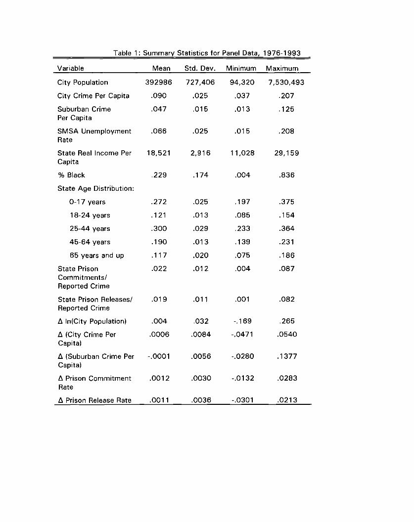
Table 1: Summary Statistics for Panel Data, 1976-1993

Variable Mean Std. Dev. Minimum Maximum

City Population

City Crime Per Capita

Suburban Crime

Per Capita

SMSA Unemployment

Rate

State Real Income Per

Capita

O\OBlack

State Age Distribution:

0-17 years

18-24 years

25-44 years

45-64 years

65 years and up

State Prison

Commitments/

Reported Crime

State Prison Releases/

Reported Crime

A In(City Population)

A (City Crime Per

Capita)

A (Suburban Crime Per

Capita)

A Prison Commitment

Rate

A Prison Release Rate

392986

.090

.047

.066

18,521

.229

.272

.121

.300

.190

.117

.022

.019

.004

.0006

-.0001

.0012

.0011

727,406

.025

,015

.025

2,916

.174

.025

,013

.029

.013

.020

.012

.011

.032

.0084

.0056

.0030

.0036

94,320

.037

.013

.015

11,028

.004

,197

.085

.233

.139

.075

.004

.001

-.169

-,0471

-.0280

-.0132

-.0301

7,530,493

.207

.125

.208

29,159

.836

.375

.154

.364

.231

.186

.087

.082

.265

.0540

.1377

.0283

.0213

Notes to Table 1: Sample is comprised of annual observations from 1976-1993 for 137

U.S. central cities with population greater than 100,000 in population in 1975. Due to

occasional missing data, number of observations is equal to 2,165. Prison commitment

and release data are defined at the state level and are changes in rates per reported crime.

All other data are defined at the city level unless otherwise noted. All variables are

available annually except YO high school graduates, YO home-owners, YO manufacturing, and

0/0 black, which are available only in census years. % black is linearly interpolated between

decennial census years.

Table 2: OLS Estimates of the Relationship Between City Population and Crime Rate

Variable (1) (2) (3) (4) (5) (6)

A (Per Capita

City Crime)

A (Per Capita

Suburban Crime)

Per Capita City

Crime (-1 )

Per Capita

Suburban Crime (-1 )

Unemployment Rate

(-1)

State Per Capita

lncome*l Os (-1)

YO black (-1 )

YO aged 0-17 (-1)

% aged 18-24 (-1)

YO aged 25-44 (-1 )

YO aged 45-64 (-1 )

‘AA state populationf-l)

-1.039

(.076)

.539

(.104)

----

----

-.045

(.032)

.11

(.57)

-.034

(,004)

-.031

(.085)

.568

(.127)

-.045

(.076)

.207

(.151)

.543

-1.035

(.075)

.525

(.104)

----

----

-.139

(.050)

.43

(1.28)

.028

(.039)

-.594

(.177)

-.668

(.286)

-.952

(.260)

-.601

(.242)

.634

-1.135

(.0786)

.424

(.105)

----

----

-.228

(.058)

.38

(2.48)

-.019

(.042)

-.193

(.280)

-.285

(.396)

-.704

(.362)

-.073

(.410)

.356

(.191)

-.992

(.078)

.448

(.108)

.002

(.032)

-.046

(.056)

-.046

(.032)

.24

(.58)

-.033

(.005)

-.046

(.086)

.504

(.133)

-.086

(.078)

.167

(.154)

.560

-1.024(.082)

.499

(.121)

-.058

(.066)

.082

(.127)

-.146

(.050)

.48

(1.30)

.039

(.039)

-.574

(.180)

-.723

(.295)

-.949

(.267)

-,631

(.257)

.644

-1.123

(.086)

.440

(.124)

-.052

(.069)

,148

(,134)

-.232

(.062)

.64

(2.54)

-.014

(.043)

-.107

(.283)

-.416

(.401)

-.689

(.369)

.023

(.418)

.334

-, (.096) (.124) . . (.097) (.129) (.194)

City Fixed Effects? No Yes Yes No Yes Yes

Region-year

interactions No No Yes No No Yes

R-squared .310 .390 .490 .315 .393 .495

Notes: Dependent variable is Aln(city population). Sample is comprised of annual

observations from 1976-1993 for 137 U.S. central cities with population greater than

100,000 in population in 1975. Number of observations is equal to 2,165 in all columns.

Year and region dummies are included in all columns except those where region-year

interactions are present. All variables are available annually, except for YO black, which is

linearly interpolated between decennial census years. See Table 1 for further information

about the level of geographic disaggregation of the covariates. Estimates control for

heteroskedasticity by city size. Standard errors in parentheses.

Table 3: First-stage and Reduced-form Estimates of State Prison Commitments and

Releases on Crime Rates and Citv Populations

A per capita city crime 0/0A city population

Variable (1) (2) (3) (4) (5) (6)

A Prison

Commitments Per

Crime (-1)

A Prison

Commitments Per

Crime (-2)

A Prison Releases

Per Crime (-1 )

A Prison Releases

Per Crime (-2)

Unemployment

Rate* 100 (-1)

State Per CapitaIncome*IOG (-1]

‘A black (-1)

YO aged 0-17 (-1)

YO aged 18-24 (-1 )

YO aged 25-44 (-1 )

YO aged 45-64 (-1 )

O\OAstate populationi-l)

-.405

(.085)

-.192

(.095)

.413

(.076)

.303

(.014)

-.003

(.009)

.23

(.16)

.003

(.001)

.007

(.023)

-.057

(.036)

-.038

(.021)

-.016

(.042)

-,052

-.393

(.087)

-.173

(.097)

.407

(.078)

.300

(.076)

-.008

(.014)

.66

(.36)

.010

(.011)

.009

(.051)

-.119

(.084)

-.073

(.077)

-.020

(.070)

-.084

-.283

(.108)

-.027

(.117)

.282

(.090)

.157

(.091)

-.052

(,017)

.06

(.07)

.001

(.012)

-.044

(.076)

-.019

(.111)

-.091

(.101)

-.360

(.110)

-.023

.457

(.300)

.988

(.336)

-,689

(.270)

-.464

(.262)

-.041

(.032)

-.14

(.55)

-.035

(.004)

-.025

(.083)

.601

(.126)

.013

(.074)

.236

(.147)

.616

,317

.295)

.945

.330)

.742

(.264)

-.544

(.256)

-.129

(.048)

.34

( 1.20)

.034

(.037)

-.546

(.171)

-.577

(.283)

-.742

(.258)

-.486

(.239)

.718

.274

(.368)

.999

(.404)

-.703

(.312)

-.857

(.311)

-.187

(.061)

-1.95

(2.36)

-.005

(.039)

-.284

(.267)

-.278

(.390)

-.391

(.353)

.519

(.386)

.349

,., (.027) (.036) (.055) (.031) (,123) (.189)

City Fixed Effects? No Yes Yes No Yes Yes

Region-Year No No Yes No No Yes

Interactions?

p-value: instruments <.001 <.001 .01 .034 .021 .048

R-squared .280 .294 .429 .257 .334 .426

Notes to Table 3: Dependent variables are changes in per capita city crime in columns 1-3

and Aln(city population) in columns 4-6. Sample is comprised of annual observations from

1976-1993 for 137 U.S. central cities with population greater than 100,000 in population

in 1973. Year and region dummies are included in all specifications. Due to missing data,

number of observations is equal to 2,301 in columns 1-3 and 2,412 in columns 4-6. Prison

commitment and release data are defined at the state level and are changes in rates per

reported crime. All variables are available annually, except for % black, which is linearly

interpolated between decennial census years. See Table 1 for further information about the

level of geographic disaggregation of the covariates. Estimates control for

heteroskedasticity by city size. Standard errors in parentheses. The bottom row of the

table gives the joint significance of an F-test of the four prison variables.

Table 4: 2SLS Estimates of the Impact of Crime on City Population

Cities <470 Cities>4%All cities in sample of state pop. of state pop.

Variable (1) (2) (3) (4) (5)

A (Per Capita City

Crime)

A (Per Capita

Suburban Crime)

Unemployment Rate

(-1)

State Per Capita

lncome*l OG (-1)

YO black (-1 )

% aged 0-17 (-1)

YO aged 18-24 (-1 )

YO aged 25-44 (-1 )

YO aged 45-64 (-1 )

O\OAstate population(-1)

-1.34

(.59)

.67

(.19)

-.044

(.032)

.16

(.59)

-.032

(.005)

-.042

(.086)

,568

(.132)

-.053

(.079)

.185

(.154)

.517

(.103)

-1.43

(.57)

.68

(.19)

-.137

(.051)

.66

(1.37)

.037

(.040)

-.584

(.180)

-.671

(.297)

-.989

(.270)

-.646

(.247)

.592

(.134)

-2,03

(.92)

.68

(.23)

-.261

(.073)

1,15

(2.71)

-.021

(.044)

-.266

(.297)

-.337

(.41 6)

-.930

(.409)

-.481

(.583)

.330

(.200)

-2.60

(1.57)

1.27

(.79)

-.080

(,088)

5.92

(4,86)

.025

(,081)

-.946

(.667)

-,996

(1 .238)

-1.432

(.889)

-.106

(.870)

-.161

(.418)

-1.64

(1.23)

.51

(.26)

-.431

(.131)

.24

(3.96)

-.082

(.068)

-.120

(.420)

-.339

(.616)

-.970

(,581)

-.280

(.847)

.284

(.278)

City Fixed Effects? No Yes Yes Yes Yes

Region-year No No Yes Yes Yes

interactions

p-value: .135 .070 .039 .346 .035

overidentifying

restrictions

Number of Ohs. 2,140 2,140 2,140 1,183 957

Notes: Dependent variable is Aln(city population), Sample is comprised of annual observations from1976-1993 for 137 U.S. central cities with population greater than 100,000 in population in 1973.Year and region dummies are included in all specifications except those where region-yearinteractions are present, Once- and twice-lagged state prison commitment and release rates per

crime are used as instruments in all columns. The P-value of an NR2 test of overidentifyingrestrictions on instruments is reported in table. All variables are available annually, except for YO

black, which is linearly interpolated between decennial census years. Estimation allows forheteroskedasticity by city population. Standard errors in parentheses.

mmo:g:. . .

u

0s(00. .-m

c.-5.-

3

Table 8a: Household-level Estimates of the Decision to Stay in Central Cities

MiddleVariable All Household Heads High Income Income Low Income

A Per Capita Crime in City -1.61

(.72)

-1.40

(.56)

1.03

(.83)

-.009

(,001)

-1.59

(.632)

.797

(1 .02)

-.007

(.001)

-1.53

(.637)

1.12

(.970)

-.011

(.001)

.007

(.001)

.030

(.003)

.149

(.020)

.018

(.005)

-.037

(.004)

.015

(.024)

-.277

(.018)

-.082

(.008)

-1.15

(.465)

1.17

(.678)

-.008

(.0004)

.005

(.0004)

.017

(.003)

.132

(.019)

.046

(.008)

-.050

(.005)

.036

(.015)

-.267

(.030)

-,090

(.010)

A Per Capita Suburban

Crime

Years of Education

1.61

(1.01)

Income Group:

Middle .018

(.005)

.024

(.009)

.006

(.001)

.027

(.002)

.148

(.019)

.022

(.005)

-.036

(.004)

.014

(.024)

-.276

(.019)

-,100

High

Age .010(.001)

.025

(.006)

.159

(.01 9)

.014

(,006)

-.023

(.009)

-.013

(.042)

-.229

(.023)

-.100

Male

Black

Has Own Children

Married

Homeowner

Armed forces 1975

College student 1975

(.009) (.01 o)

Controls from City-level Yes Yes Yes Yes Yes

Regressions

R-squared .029 .152 .158 .155 .142

Observations 402042 402042 73277 197089 131676

Comparable Coefficient from City-level Regression

A Per Capita Crime in City -1,50 -1.50 -1.96 -1.62 -1.07

(.74) (.74) (.90) (.86) (.61)

Notes to Table 8a: The sample includes only households residing in one of the 81 central cities included in

the sample in 1975. The dependent variable is an indicator equal to one if the household remains in the

central city in 1980, and zero otherwise. The complete set of state and city-level regressors are included

in these specifications: state real per capita income and age distribution variables in 1975, state

population growth 1975 to 1980, SMSA unemployment rate 1975, city YO black, YO graduating high

school, ‘A housing owner occupied, median family income in 1970, ‘A manufacturing, mean hourly wagein manufacturing, YO multi-family housing, climate controls, and region dummies. We allow for correlation

in the error term across households in a given city so as not to understate the standard errors.

Table 8b: Household-level Estimates of the Decision to Stay in Central Cities (Con’t)

Non-

Variable Black Black With Children No Children

A Per Capita Crime in City -1.72 -1.34 -1.80 -1.14(.59) (.599) (.635) (.528)

A Per Capita Suburban 2.32 1.04 1,47 .641

Crime (1.21) (.930) (.982) (.837)

Years of Education -.007 -.010 -.013 -.007

(.001) (.001) (.001) (.001 )

Income Group:

Middle -.003

(.006)

.026

(.005)

-.006

(.005)

.023

(.005)

High -.008

(.009)

.033

(.010)-.010

(.010)

.032

(.010)

Age

Male

Black

.004

(.0003)

.006

(.001)

.009

(.001)

.006

(.001)

.024

(.003)

.024

(.003)

.052

(.007)

.017

(.003)

.166

(.026)

.129

(.014)

Has Own Children .033

(.005)

.013

(.006)

Married -.028

(.003)

-.038

(.005)

-.030

(.004)

-.032

(,003)

Homeowner .019

(.016)

.016

(.026)

-.010(.030)

.028

(.021)

-.287

(.018)-.270

(.837)Armed forces 1975

College student 1975

-.198

(.025)

-.258

(.016)

-.083 -.100 -.056 -.117

(.010) (.009) (.010) (.010)

Control from City-level Yes Yes Yes Yes

Regressions

R-squared .094 .146 .144 .158

Observations 88360 313682 135787 266255

Comparable Coefficient from City-level Regression

A Per Capita Crime in City -.47 -1.35 -1.99 -1.24

(.85) (.80) (.85) (.69)

Notes: See notes to Table 8a.

Biblioara~hv

Beattie, John, 1995, “Crime and Inequality in Eighteenth-Century London, ” in Crime andIneaualitv, J. Hagan and R. Peterson (eds.), Stanford: Stanford University Press.

Benabou, Roland, 1993, “Workings of a City: Location, Education, and Production, ”

Quarterly Journal of Economics 108:619-652.

Bergstrom, Theodore and Robert Goodman, 1973, “Private Demands for Public Goods, ”

American Economic Review 63:280-296.

Blanchard, Olivier and Lawrence Katz, 1992, “Regional Evolutions, ” Brookings Papers on

Economic Activity, 1-61.

Blanchard, Olivier and Lawrence Summers, 1987, “Fiscal Increasing Returns, Hysteresis,

Real Wages, and Unemployment, ” European Economic Review 31:543-566.

Bradbury, Katharine, Anthony Downs, and Kenneth Small, 1982, Urban Decline and the

Future of American Cities, Washington, DC: Brookings.

Bradford, David, and Harry Kelejian, 1973, “An Econometric Model of the Flight to the

Suburbs, ” Journal of Political Economy 81:566-589.

Bureau of Justice Statistics, 1994, Criminal Victimization in the United States , 1992,

Washington DC: Bureau of Justice Statistics.

Case, Anne and Lawrence Katz, 1991, “The Company You Keep: the Effects of Family and

Neighborhood on Disadvantaged Youths, ” NBER Working Paper.

Cohen, Mark, 1988, “Pain, Suffering, and Jury Awards: A Study of the Cost of Crime toVictims, ” Law and Society Review 22:537-555.

Cutler, David and Edward Glaeser, 1995, “Are Ghettos Good or Bad?” NBER Working

Paper.

Dilulio, John, and Anne Piehl, 1991, “Does Prison Pay? The Stormy National Debate over

the Cost-effectiveness of Imprisonment, ” The Brookings Review (fall), 28-35.

Frey, William H., 1979, “Central City White Flight: Racial and Nonracial Causes, ” American

Sociological Review 44:425-448.

Glaeser, Edward, and Bruce Sacerdote, 1996, “Why is There more Crime in Cities, ” NBERWorking Paper No.5430.

Glendon, Spencer, 1996, “Metropolitan Housing Choice: Families, Crime, and Social

Interactions, ” Mimeo, Harvard University.

Gonzalez, Rudolfo and Stephen Mehay, 1987, “Economies of City Size in a Price Searcher

Model of Local Government, ” Public Finance 42:236-249,

Gottdeiner, Mark (editor), 1986, Citie s in Stress : A New Look at Urban Crisis, Beverly Hills:

Sage.

Grubb, W. Norton, 1982, “The Flight to the Suburbs of Population and Employment, 1960-

70, ” Journal of Urban Economics 11:348-367.

Hellman, Daryl and Joel Naroff, 1979, “The Impact of Crime on Urban Residential Property

Values, ” Urban Studies 16:105-112.

Inman, Robert, Steven Craig, and Thomas Lute, 1994, “The Fiscal Future for American

Cities: Lessons from Three Cities, ” Research Impact Paper #4, Wharton Real Estate

Center, University of Pennsylvania.

Katzman, Martin, 1980, “The Contribution of Crime to Urban Decline, ” Urban Studies

17:277-286.

Ladd, Helenr and Katherine Bradbury, 1988, “City Taxes and Property Tax Bases, ” /Vationa/

Tax Journal 41:503-523.

Ladd, Helen, and Julie Boatright Wilson, 1983, “Who Supports Tax Limitations: Evidence

from Massachusetts’ Proposition 2 k ,“ Journal of Policy Analysis and Management

2:256-279.

Levitt, Steven, 1995, “The Relationship between Crime Reporting and Police: Implications

for the Use of Uniform Crime Reports, ” Mimeo, Harvard University.

Levitt, Steven, 1996, “The Effect of Prison Population Size on Crime Rates: Evidence from

Prison Overcrowding Litigation, ” Quarterly Journal of Economics 111:319-352.

Marshall, Harvey, 1979, “White Movement to the Suburbs: A Comparison of

Explanations, ” American Sociological Review 44:975-994.

Marshall, Harvey, and Kathleen O’Flaherty, 1987, “Suburbanization in the Seventies: The

‘Push-Pull’ Hypothesis Revisited, ” Journal of Urban A ffairs 9:249-262.

Marvell, Thomas and Carlisle Moody, 1994, “Prison Population Growth and Crime

Reduction, ” Journal of Quantitative Criminology 10:109-140.

Miller, Ted, Mark Cohen and Shelli Rossman, 1993, “Victim Costs of Violent Crime and

Resulting Injuries, ” Health Affairs 12:186-197.

Monkkonen, Eric, 1981, Police in Urban America, 186 0-1920, New York: Cambridge

University Press.

O’Brien, Robert, 1985, Crime and Victimiz ation Data, Beverly Hills: Sage.

Sampson, Robert J. and John D. Wooldredge, 1986, “Evidence that High Crime Rates

Encourage Migration Away from Central Cities, ” Sociology and Social Research

90:310-314.

Schwartz, Joe, 1987, “On the Road Again, ” American Demographics 9 (April) :38-42.

Smith, Barton, 1978, “Measuring the Value of Urban Amenities, ” Journa/ of Urban

Economics 5:370-387.

Smith, D. R., and G.R. Jarjoura, 1988, “Social Structure and Criminal Victimization, “Social

Structure and Criminal Victimization, ” Journal of Research in Crime and Delinquency

25:27-52.

Spelman, Williamr 1994, Criminal lnca~ac itation, New York: Plenum.

Taeuber, Karl and Alma Taeuber, 1964, “White Migration and Socioeconomic Differences

between Cities and Suburbs, ” American Socio/ogica/ Review 29:718-729.

Taylor, R. and J. Covington, 1988, “Neighborhood Changes in Ecology and Violence, ”

Criminology 26:553-590.

Thaler, Richard, 1978, “A Note on the Value of Crime Control: Evidence from the Property

Market, ” Journal of Urban Economics 5:137-145.

U.S. Bureau of the Census, 1993, Citv G overnment Finances : 1990 -1991, Series GF/91 -4,

Washington, DC: U.S. Government Printing Office.

Wilson, William Julius, 1987, The Trulv Disadvantage d: The Inner Citv, the Underclass, and

Public Policv, Chicago: University of Chicago Press.

Yinger, John and Helen Ladd, 1989, “The Determinants of State Assistance to Central

Cities, ” National Tax Journal 42:413-428.