Flight from Urban Blight:Lead Poisoning, Crime and Suburbanization

Federico Curci∗ and Federico Masera†‡

November 9th 2017

Job market paper

Abstract

In the post World War II period, most U.S. cities experienced large movementsof population from the city centers to the suburbs. In this paper we providecausal evidence that this process of suburbanization can be explained by the riseof violent crime in city centers. We do so by proposing a new instrument to ex-ogenously predict violent crime. This instrument uses as time variation the U.S.national levels of lead poisoning. Cross-sectional variation comes from a proxyfor soil quality, which explains the fate of lead in soil and its subsequent bioavail-ability. Using data for more than 300 U.S. cities, results show that the increase inviolent crime from the level in 1960 to its maximum in 1991 decreased the pro-portion of people living in city centers by 15 percentage points. This increase incrime moved almost 25 million people to the suburbs. As a result of suburbaniza-tion, we find that people remaining in the city center are more likely to be blackpeople, consistent with the “white flight" phenomenon. We then demonstratethat this suburbanization process had aggregate effects on the city. Exploiting aspatial equilibrium model, we determine that violent crime had externalities onproductivity and amenities.

∗Universidad Carlos III de Madrid. E-mail: fcurci@eco.uc3m.es.†University of New South Wales. E-mail: f.masera@unsw.edu.au‡Curci thanks Ricardo Mora for the excellent supervision. We thank Nathaniel Baum-Snow, Stephen

Billings, Julio Cáceres, Irma Clots-Figueras, Klaus Desmet, Jesús Fernández-Huertas, Pauline Grosjean,Adelheid Holl, Matthias Kredler, Salvatore Lo Bello, Olivier Marie, Florian Mayneris, Jaime Millán, LuigiMinale, Peter Nillson, William Parienté, Nishith Prakash, Michele Rosenberg, Kevin Schnepel, WilliamStrange, Jan Stuhler, Bruno Van der Linden, Gonzague Vannorenberghe, and Hasin Yousaf for relevantinputs and comments. We also thank participants to the UC3M reading group, UC3M PhD workshopand 17th SAET Conference on Current Trends in Economics, and seminars at Université Catholique deLouvain, University of New South Wales, Stockholm University and Università Commerciale Bocconi.Financial support from the Spanish Ministry of Economics and Competitiveness (ECO2012-33053) isacknowledged.

1

1 Introduction

In the last century, both developed and developing countries experienced at the sametime two important urban phenomena: urbanization and suburbanization. Urban-ization refers to the movement of people from rural to urban areas. Suburbanizationrepresents the movement of population from city centers to low density suburban ar-eas. The increase in the number of people living in the suburbs is not just caused bycity growth, as shown by Angel et al. (2011). U.S. cities provide an emblematic exam-ple of this suburbanization process. According to Baum-Snow (2007), U.S. populationliving in city centers declined by 17 percent between 1950 and 1990 despite popula-tion growth of 72 percent in metropolitan areas.

The advantages and drawbacks of city growth have been largely studied. Urban-ization reflects agglomeration economies and higher productivities. At the same time,large cities might suffer congestions and urban distress. In particular, crime is higherin bigger cities (Glaeser and Sacerdote, 1999). The movement of people from city cen-ters to suburbs can underline the negative effects of density. In this paper we providenovel causal evidence for a mechanism that links the increase in violent crimes in U.S.city centers between the 1960s and the 1990s to suburbanization. We then show theconsequences of this reallocation of people within cities in terms of racial segregation,and overall city productivity and amenities. Suburbanization of people has implica-tions in terms of congestions and transport costs, decreasing amenities in cities. Italso affects location of firms and then city productivity. Therefore, in this paper weshow that suburbanization is crucial to explain how city structure can influence pro-ductivity and amenities externalities offered by cities, something that has received theattention of a limited number of studies.

While in 1960, 43% of the urban population in the U.S. was living in city centers,this proportion dropped to 33% in 1990. In this paper, we argue that the amenity valueof city centers in the U.S. decreased because of crime, leading people to suburbanize.In fact, U.S. cities experienced a dramatic increase in violent crimes at the same timethat population suburbanized (see Figure 1(a)). The violent crimes rate rose from 23crimes per 10,000 inhabitants in 1960 to 163 crimes per 10,000 inhabitants in 1991.Similarly, cities in which violent crime increased the most had the strongest decreasein proportion of people living in city centers (see Figure 1(b)). When crime rates de-creased, after 1991, the general trend for suburbanization did not revert.1

[INSERT FIGURE 1 HERE]The goal of this research is to provide causal evidence and to quantify the effect of

crime on suburbanization. We do so by proposing a new instrument to exogenouslypredict violent crime rate in the city centers of all U.S. cities. The time variation of ourinstrument is provided by U.S. national levels of lead consumption. Medical litera-ture recognizes that exposure to lead as a child alters the formation of the brain andincreases aggressive behaviour in adulthood. We exploit the specific timing of the ef-fect of lead on crime to be sure that we are not capturing the effect that lead mighthave on other outcomes. Lead emissions by cars in the U.S. increased dramatically

1There are some recent studies that provide evidence of the return of some categories of populationto city centers, in particular white people with college degree (see Baum-Snow and Hartley, 2016 for areview). However, these individuals represent a small proportion of the U.S. population.

2

until 1972, and 19 years later crime rates reached their peak. Given that our identifi-cation strategy takes advantage of this increase in lead exposure, we concentrate ouranalysis on the period between 1960 and 1991. Lead emissions by cars accumulate inthe soil and then can be ingested by humans via soil resuspension. We obtain geo-graphical variation for our instrument by exploiting the chemical literature evidenceshowing that lead bioavailability to humans increases when lead deposits in soils of aparticular pH level. We use this information to instrument violent crime rates usingthe interaction between the lagged national level of tetraethyl lead used in cars and afunction of the pH of the soil. We construct this instrument using machine learningtechniques as described in Section 4.2.

We estimate the effect of violent crime on suburbanization using a newly assem-bled database for more than 300 U.S. cities. Our results show that the increase inviolent crimes from the level of 1960 to their maximum in 1991 was responsible fora decrease in the proportion of people living in city centers by 15 percentage points.Increases in violent crime led more than 25 million people to leave city centers. How-ever, we encounter that the increase in crime rate did not change the total city pop-ulation. Higher crime rates in the city centers drove people to relocate within citiesbut not between cities. We also find that this suburbanization process was associatedwith the so-called "white flight". As a city center became more violent, white peoplemoved to the suburbs, leading to an increase in the percentage of black people in thecity center. Moreover, we provide evidence that the increase in violent crime was notonly responsible for residential suburbanization but also it induced firms to leave citycenters and locate in the outskirts of the city. Employment decentralization followedresidential suburbanization and not the opposite. These results are confirmed afterseveral robustness and specification tests.

After showing that violent crime had an effect on the distribution of people andfirms inside a city we explore whether this phenomenon generated aggregate effectsat the city level. In addition to finding that violent crime did not decrease the over-all population of the city, we prove that violent crime increased both house pricesand median incomes. To rationalize these city-aggregate results, we estimate a spa-tial equilibrium model, based on Glaeser (2008), in which people decide in which cityto locate and in equilibrium utility should be equalized between cities. We assumethat violent crime can affect city amenities and productivity. We exploit the modelto map reduced form elasticities of the effect of violent crime on house prices, wagesand total city population, to structural parameters that describe the effect that vio-lent crime has on city amenities and productivity. We find that higher violent crimerates and the consequent relocation of people inside a city decrease city amenitiesbut increase overall city productivity. Our structural estimates imply that the increasein violent crime in the city center between 1960 and 1991 led to a decrease in the av-erage amenities of the city of 23.2%. We provide suggestive evidence that the effect ofcrime on productivity is entirely caused by the effect that crime has on employmentdecentralization.

This paper first contributes to the literature about the determinants of suburban-ization. Several reasons have been identified as contributors of the suburbanizationof U.S. cities. Causal evidence of the effect of highways on suburbanization has been

3

provided by Baum-Snow (2007).2 Brueckner and Rosenthal (2009) argue that subur-banization is explained by the fact that high-income households have higher demandfor newer housing stock, which develops faster in suburban locations. Boustan (2010)shows that the large migration of black population from the rural South of the U.S. ledto whites leaving the cities. Reber (2005) provides evidence that white flight has beenstronger in districts with court-ordered desegregation plans.3 Several early studieshave more generally related urban blight to the flight from city centers.4

We show that the increase in crime rates from the 1960s to the 1990s is an impor-tant reason for U.S. suburbanization. According to our estimates, the relative increasein crime between city centers and suburbs from 1960 to 1991 implies a 35% decreasein the population of city centers. We can compare this result to similar numbers inthe literature. Baum-Snow (2007) provides evidence that the construction of the in-terstate highway system reduced the population of city centers by 23%. The effect ofthe great black migration has been estimated to cause a drop in 17% in city centerpopulation (Boustan, 2010). In this paper, we demonstrate that the effect of violentcrime has important complementarities with these other mechanisms. In fact, weshow that the increase in violent crime rates increased the construction of highwaysand decreased the white population in the city centers, which consecutively furtherinfluenced suburbanization. We also find that the suburbanization caused by crime isstronger in cities with more blacks in the city center and in cities with more highways.

The link between crime and relocation of people has been the object of studyof a limited amount of analyses. Cullen and Levitt (1999) were the first to causallyconsider the relationship between crime rates and city population. Their empiricalstrategy consists of analyzing the effect on a city center population of crime rates in-strumented by the lagged changes in the punitiveness of the state criminal justicesystem and controlling for city and year fixed effects and several city characteristics.They conclude that the decrease in city population because of increased crime ratesis mainly due to people migrating out of the city center. Our work differs from Cullenand Levitt (1999) because we exploit exogenous variation at a much finer geographi-cal level of observations that do not correlate with any potential suburbanization con-founding mechanism at city level.

Our findings relate to the growing literature on optimal city structure. These stud-ies rely on the classical urban models developed by Alonso (1964), Mills (1972), andMuth (1969), and subsequently expanded by Fujita and Ogawa (1982), Lucas andRossi-Hansberg (2002), Ahlfeldt et al. (2015), and Allen et al. (2015). Our work alsoconnects to studies about how urban amenities change in response to urban shapeand crime. The cornerstone of these works is the spatial equilibrium concept intro-duced by the seminal works by Rosen (1979) and Roback (1982), and then reviewedby Glaeser (2008) and Moretti (2011). Similar to our work, Harari (2015) estimatesthe externality effects of urban compactness. Diamond (2016) shows that crime is an

2Similar evidence has been found for the case of Spain (Garcia-Lopez et al., 2015) and other Euro-pean countries (Garcia-Lopez et al., 2015). Similarly, Glaeser and Kahn (2004) and Kopecky and Suen(2010) relate suburbanization to car adoption.

3This last result was not confirmed by Baum-Snow and Lutz (2011) who find that school desegrega-tion affected only out-of-city migration and not within-city suburbanization.

4See, for example, Bradford and Kelejian (1973), Frey (1979), Grubb (1982), Mieszkowski and Mills(1993), and Mills and Lubuele (1997). Cullen and Levitt (1999) look specifically at the role of crime.

4

important component of urban amenities, which then influences location of people.We contribute to these literatures by showing that the effect of crime on employmentdecentralization creates externalities over city amenity and productivity.

Our paper also contributes to a long-standing stream of literature that studies thedeterminants of violence and crime.5 In particular, we relate to the strand of this liter-ature that studies the biological determinants of violence. As reviewed by Rowe (2002)and O’Flaherty and Sethi (2015) there is a growing body of evidence on how genetic,medical and environmental factors may increase the propensity of violent behavior.In particular, we build on a medical literature that has shown how lead poisoning isa potent neurotoxin that is closely related to aggressive and violent behavior. In eco-nomics, there is a new and growing stream of literature that studies the relationshipbetween lead poisoning and crime (see Section 4.1 for a review of the literature). Wecontribute to this literature by exploiting a new source of cross-sectional variationgiven by the type of soil in a city. We then use this new instrument to provide causalevidence of the effect lead poisoning from resuspended lead has on violent crime.

Moreover, we contribute to the literature that studies the effects of crime. Here,the literature has mainly focused on the detrimental effects that a violent environ-ment has on the young, especially when it comes to their educational decisions (Bowenand Bowen, 1999; Henrich et al., 2004). Another important strand of the literature hasinstead looked at the effects crime has on economic activity, mainly by deterring in-vestments (Daniele and Marani, 2011; Detotto and Otranto, 2010). In this paper, weprovide causal evidence of the effects that crime has on suburbanization and how thisshapes the location of people inside a city.

Finally, our work is one application of machine learning for construction of in-strumental variables (see Athey and Imbens, 2017 for a review). We select a proxy ofsoil quality between a large set of possible alternatives using an algorithm that findsthe instrument that maximizes the relevance condition. We run the first stage of ourregression for any possible interval of soil pH and we select the interval that maxi-mizes the F-statistics. We then show how the pH of the soil selected by this algorithmconforms to what is expected by the chemical literature. We argue that the soil qual-ity index selected is in line with the identification assumption required for exogeneityand we show that the results are robust to the use of other proxies.

This paper is structured as follows. Section 2 discusses the empirical strategy toobtain the causal effect of crime on suburbanization. Section 3 describes the dataused. The instrumental variable and the identifying assumptions are explained inSection 4. Empirical results are reported and discussed in Section 5. Section 6 exam-ines the possible threats to identification and provide evidence of the robustness ofthe results. In Section 7, we present the spatial equilibrium model and estimates ofthe externality effects of crime rates on amenities and productivity. Lastly, Section 8concludes.

5Most of the efforts in this literature have been concentrated in assessing the effect of police, in-carceration and the judicial system on the criminal activity (for the most recent literature review, seeChalfin and McCrary, 2017). Another strand of the literature instead has been focused on how differentsocial and economic circumstances may affect crime. Examples of these determinants are income in-equality (Kelly, 2000), immigration (Bianchi et al., 2012), gun laws (Ludwig, 1998) and social cohesion(Goudriaan et al., 2006) among many others.

5

2 Empirical strategy

The empirical model we want to estimate is reported in Equation 1. Our objective isto understand the effect of the increase in violent crimes per capita (VC) in the citycenter (cc) of one metropolitan area (m) in a particular year (t) on the suburbaniza-tion of that city. The proxy for suburbanization (subm,t ) we use is the proportion ofpopulation living in the city center (popcc ) over the total city population, which isthe sum of the population in the city center and in the suburbs (popncc ). In orderto control for unobserved heterogeneity we introduce both metropolitan area (MSA)and year fixed effects, τm and τt , respectively. We also include geographic (g) specifictime trends, i.e. τg ×τt . In our preferred specification we impose Census District timetrends (discussion of these time trends is presented in Section 4.3).

subm,t =popcc

m,t

popccm,t +popncc

m,t= τm +τt +βV C cc

m,t +τg ×τt +εm,t (1)

The OLS estimation of the coefficient of the effect of violent crime on suburban-ization, β can suffer different biases. Firstly, reverse causality might be present sincemore suburbanized cities might have poorer city centers, which in turn can increasecrime rates in the city center. Evidence of this reverse causality has been found byJargowsky and Park (2009). Moreover, omitted variable biases can contribute to theinconsistency of our estimation. One possible omitted variable is the proportion ofblack people living in the city center. Boustan (2010) shows that part of the whiteflight has followed the influx of black population in the city. This estimation can alsosuffer omitted variable bias if cities with more highways tend to have higher level ofcrimes.

We propose a new instrument that, we argue, can exogenously predict crime atcity center level: the interaction between the lagged amount of the tetraethyl lead (TL)used in car gasoline in the U.S. and a proxy for the bioavalability of lead to humansin the ciy centers. Lead has an effect of brain development of children, and increasetheir aggresive behaviour. The highest potential of delinquency is reached at 19 yearsold.6 Hence, for any given year, we use tonnes of tetraethyl lead in cars 19 years beforeto predict crime rates. Section 4.1 discusses in details the relationship between leadand crime.

Lead adsorption in the soil depends on particular soil characteristics. Bioavail-ability of lead is proxied by a specific function of the average pH of the soil in thecity center. In particular, our soil bioavailability indicator is a dummy variable takingvalue 1 if the average pH of the soil is between the values of 6.8 and 7.7. We obtain thisproxy using a machine learning algorithm described in Section 4.2. The first stage ofour instrumental variable estimation is reported in Equation 2. One of the main ad-vantages of our instrument is that it varies both in space and time, therefore we caninclude year and city fixed effects in our first stage.

V C ccm,t =µm +µt +χT Lt−19 × 1

(6.8 ≤ pH cc

m ≤ 7.7)+µg ×µt +εm,t (2)

6According to United States Department of Justice (1993) in 1965 people with 19 years old had thehighest arrest rates for violent crimes.

6

3 Data

We have assembled an unique database for 306 city centers from 1960 to 2014 in theU.S. combining different data sources. The first data source we use is the F.B.I. Uni-form Crime Reporting (UCR) Program Data (United States Department of Justice).For each local enforcement agency, which is coded by a Originating Agency Iden-tifier (ORI) number, this data source provides information about monthly numberof crimes for each year for all different kind of crimes.7 This database also reportsthe total jurisdictional population under responsibility of that particular ORI. We usethis information to compute our suburbanization measure.8 We use the F.B.I. defi-nition of violent crime, that is the sum of murder and non-negligent manslaughter,total robberies, forcible rape, and aggravated assaults.9 We use the Law EnforcementAgency Identifiers Crosswalk database to link ORIs to Census Geographic Definitions(National Archive of Criminal Justice Data, 2006). We keep geography fixed at 2000definition and we aggregate all the information at U.S. Place level.10

We merge our database with the data provided by Baum-Snow (2007). This databasecontains information of several social and economic characteristics of MetropolitanStatistical Area (MSA) and city centers.11 Moreover, we use the definition of city cen-ters provided by Baum-Snow (2007), that is for each MSA he defines the city center asthe U.S. Place with the largest population in 1950.12 Therefore, for every city center wecan compute its jurisdictional population, the population of the rest of places insidethe same MSA (that we call suburbs) and the population of the MSA. The suburban-ization measure we use is the population in the city center divided by the populationin the MSA. Similarly, we construct violent crime rate per capita at city center, suburb,and MSA level.

For the construction of our instrument we use two different databases. First, weuse the United States Geological Survey (U.S.G.S.) General Soil Map in order to obtain

7We aggregate monthly data to years data. If crimes were not reported for more than 9 months wereweight the number of crimes by 12 divided the number of months in which data are missing.

8F.B.I. population in Census years is very similar to the population obtained by the U.S. Census. Fornon-Census years F.B.I. produces its own population estimation. We do not believe that the possiblemeasurement error in population relates in any way with our instrument. Moreover, we also presentrobustness using only Census population data. There are some missing values in the population data,we substitute this value by the mean value of population in the ORI. This procedure does not alter inany way our results and interpretation.

9FBI defines these crime as follows. Murder and nonnegligent manslaughter:: willful killing of onehuman being by another. Robbery: taking or attempting to take anything of value from the care, cus-tody, or control of a person or persons by force or threat of force or violence and/or by putting the vic-tim in fear. Rape: penetration, of the vagina or anus with any body part or object, or oral penetrationby a sex organ of another person, without the consent of the victim. Attempts or assaults to commitrape included. Aggravated assaults: unlawful attack by one person upon another for the purpose ofinflicting severe or aggravated bodily injury. Simple assaults excluded.

10U.S. places are settled concentrations of population that are identifiable by name. They can belegally incorporated under the laws of the state in which they are located (Incorporated Places) or not(Census Designated Places, CDC). CDC boundaries are defined by the U.S. Census in cooperation withlocal or tribal officials, and they usually coincide with visible features. They are generally updated priorto each decennial census.

11Baum-Snow (2007) also keeps MSA geography constant over time using definitions from 2000.12We keep only information of ORIs inside one MSA. We drop all the ORIs belonging to multiple

counties at the same time. We only keep observations of municipal jurisdiction crime.

7

information about the soil pH (United States Department of Agriculture). We use aspH measure the negative logarithm to the base 10 of the hydrogen ion activity in thesoil using the 1:1 soil-water ratio method representative value. For every U.S. CensusPlace we compute the average pH level and information about earth slope, elevationand precipitation.13 Second, national consumption of tetraethyl lead as gasoline ad-ditive comes from the Bureau of Mines Mineral Yearbooks (United States Bureau ofMines).

Data on firms decentralization comes from United States Census County BusinessPattern (CBP) 1974-2013. This database reports the number of employed workforceand payroll for every industry and county. Data until 1998 reports information up to4 digits SIC industries, and data from 1999 onwards up to 6 digits NAICS industries.We only keep 2 digits industries.14 We identify in which county the city center of oneMSA belongs and we compute the proportion of employment in every industry in thecounty over the total employment in the same MSA. If one MSA is composed onlyby one county we assign a missing value to the proportion of employment in everyindustry in the county over the total employment in the same MSA.

Our final database encompasses more than 9,750 observations from 1960 to 1991,and 7,038 observations from 1992 to 2014. All our main discussion will focus on theperiod from 1960 to 1991. This is given by the fact that lead poisoning increased until1972, and the biggest effect on crime of lead poisoning in one year appears 19 yearslater, when affected children have the maximum probability to commit a crime. Wedevote Online Appendix E to discus what happens after 1991. In this period lead poi-soning decreased in U.S. and as a result also crime rates decreased, but at the sametime U.S. cities continue to maintain suburbanized (see Figure 1(a)). Summary statis-tics of our database from 1960 to 1991 are reported in Online Appendix A.

4 Instrumental variable

4.1 Background on lead poisoning

Lead is a heavy metal with several properties. It has high density, lasts longer and ismore malleable than iron, is resistant to corrosion, and has relative abundance. Be-cause of these characteristics lead was adopted historically for several uses: plumb-ing, solder, painting, bullets, and as a gasoline additive. According to Dapul andLaraque (2014) there are several ways through which children and adults can get ex-posed to lead. Ingestion sources are lead-based paint, contaminated water by lead

13U.S.G.S. divides the U.S. in different map areas. Every map area is composed by different soils(components), and every component is composed by multiple layers (horizons). We use informationonly at soil level, that is when the distance from the top of the soil to the upper boundary of the soilhorizon is 0. For every map unit we compute the weighted mean of pH of the components, weightingby the component percentage in the map unit. Finally, for every place we compute the weighted meanof pH of the map area, weighted by their area.

14We also aggregate data at bigger industries definitions: agriculture, good producing industries, ser-vice producing industries and other industries. We aggregate the industries as follows. Good producingindustries: Mining, Construction and Manufacturing. Service producing industries: Transportation,Communications, Electric, Gas, And Sanitary Services, Wholesale Trade, Retail Trade, Finance, Insur-ance, And Real Estate, Services

8

pipes, lead settled in soil because of leaded gasoline, paint or other industrial sources,food cultivated in contaminated soils, or leaded objects (such as children’s toys). Thetwo main inhalation sources of lead has been leaded gasoline and occupational haz-ards in the construction, soldering, painting, plumbing, automotive and ammunitionsectors.

Lead has been used since antiquity. Its use as pigment was documented in An-cient Greece and Roman pipes were largely built with lead. The use of lead for pipes,paint and as gasoline additive has followed different timing. Lead pipes were installedon a major scale in the U.S. since the late 1800s. The danger of lead pipes was increas-ingly documented in the late 1800s and early 1900s and by the 1920s many cities andtowns were prohibiting or restricting their use (Rabin, 2008). Conversely, the use oflead in paint peaked in 1920s, and then its use declined significantly (Mielke, 1999).The Lead-Based Paint Poisoning Prevention Act, which restricted the lead content inpaint, was signed in 1971, and finally lead was banned from paint in 1978.

Tetraethyl lead was mixed with gasoline from the 1920s, because it can improveengine compression by raising the octane level of gasoline. The consumption of leadedgasoline skyrocketed in post World War II because of the increase in the use of leadas antiknock gasoline additive and the increase in the number of cars. In 1965, it wasdiscovered that lead had a pollution effect on the environment (Patterson, 1965), andseveral works followed in order to prove the link between gasoline and lead pollu-tion. Patterson’s work also began an intense debate between environmentalists andthe strong industrial lead lobby. The phase-down of leaded gasoline in U.S. began in1975 when the Environmental Protection Agency (EPA) required major gasoline re-tailers to sell at least one grade of unleaded gasoline that was required to protect newcar models with catalytic converters (Nriagu, 1990). The lead phase-down contin-ued during the 1980s when the EPA set new limits for the amount of lead in gasoline.Leaded gasoline was finally banned in 1996.

A large medical and biological literature has given evidence of the health effectof lead, in particular on neurobehavioural development in children (see Roper et al.,1991 and International Programme on Chemical Safety, 1995). Lead is a potent neu-rotoxin which alters the formation of the brain and as a result influences the forma-tion of cognitive and non-cognitive skills (see Toscano and Guilarte, 2005 and Cecilet al., 2008). According to Roper et al., 1991, "Children are at higher risk for lead expo-sure because they have more hand-to-mouth activity and they absorb more lead thanadults". It has been shown that even low level exposure to lead during childhood isrelated to cognitive and behavioral outcomes, such as lower IQ, ADHD, and hyperac-tivity (see Banks et al., 1996, Canfield et al., 2003, Chandramouli et al., 2009, and Nigget al., 2010). Moreover, early age lead poisoning has been found to relate to antiso-cial behaviours, such as aggressivity, violence and impulsivity, increasing the risk ofdelinquency (see Denno, 1990, Needleman et al., 1996, and Needleman et al., 2002).Likewise, prenatal and childhood blood lead concentrations are associated with morecriminal offenses (see Stretesky and Lynch, 2001 and Wright et al., 2008). All these re-ported effect are given by the fact that lead damages neurotransmitter function in thebrain that regulate impulse control (Aizer and Currie, 2017).

The effects of lead have been object of study in several recent works in economics.Exploiting differences in road proximity and the de-leading of gasoline, Aizer and

9

Currie (2017) find a causal positive effect of lead on juvenile delinquency. The pos-itive relationship between lead and criminal behaviour has been also found by Reyes(2015a), who also exploits variation coming from the phase-down of leaded gasoline.Feigenbaum and Muller (2016) show that water pipe lead exposure increased homi-cide rates in the 1920s and 1930s, instrumenting lead exposure by city distance fromlead refineries. A second strand of works found a negative causal effect of early child-hood lead exposure on academic achievement (Aizer et al., 2016, Reyes, 2015b, Grön-qvist et al., 2016, and Ferrie et al., 2012). Similarly, Billings and Schnepel (2017) esti-mate how lead-remediation policies can reverse the negative outcomes of lead poi-soning. A last group of research identifies the positive effect of lead exposure on mor-tality in the 1920s exploiting variation from water pipe lead poisoning coming fromdifferent water acidity, measured by the water pH (Troesken, 2008, and Clay et al.,2014).

In this paper we are interested in obtaining exogenous variation of crime rates inthe U.S. in the years between the 1960s and the 1990s, a period in which the U.S. ex-perienced a dramatic increase in violent crime. We exploit the massive increase ofnational consumption of leaded gasoline and its effect 19 years later on violent crime,when poisoned children had the highest potential for delinquency. The time rela-tionship between national levels of violent crime and lagged tetraethyl lead is evidentfrom Figure 2. In fact, the increase in tetraethyl lead matches with the posterior in-crease in violent crimes, the two time series reaching their peaks in 1972 and 1991, re-spectively. We exploit official national levels of lead poisoning by gasoline publishedby United States Bureau of Mines (United States Bureau of Mines) rather than locallevels. The reason for this choice is that local lead exposure can be correlated withpotential confounders of suburbanization, such as the proportion of highways andcars in a city.

[INSERT FIGURE 2 HERE]We obtain geographical variation of the effect of lead on crime by exploiting the

fact that lead is absorbed differently by different types of soil. Lead released fromcombustion of leaded gasoline becomes airborne and accumulates in the top 1 to2 inches of soil. Evidence suggests that the bioavailability of lead in soil reaches itslowest level with a near-neutral soil pH, i.e. when the pH of the soil is around 6.5 or7 (Reddy et al., 1995, Stehouwer and Macneal, 1999 and Peryea, 2001).15 Despite theexisting evidence on the fact that the bioavailability of lead decreases between acidicand near-neutral soils, where it reaches its minimum value, we are not aware of anystudy about bioavailability in very alkaline soils (pH higher than 7.5).

Children can ingest residual lead in the soil by eating the soil or inhalating it be-cause of air dust resuspension (Laidlaw and Filippelli, 2008, Zahran et al., 2013, and

15The bioavailability of lead in soil depends on its solubility, i.e. how tightly it is held by soil parti-cles (Stehouwer and Macneal, 1999). Lead is more soluble in acidic soils (pH lower than 6.5), and it isless soluble in neutral soils (pH between 6.5 and 7.5). Lead availability is considered to be minimizedwhen the pH of the soil is higher than 6.5 or 7. This is given by the fact that the existence of solid-phase phosphates in the soil can induces the dissolution of lead mineral and its desorption. That is,the desorption of lead causes the formation of pyromorphites and the bioavailability of lead is reducedwithout its removal from the soil (Traina and Laperche, 1999). Reddy et al. (1995) conclude that mo-bility of lead will increase in environments having low pH due to the enhanced solubility of lead underacidic conditions.

10

Aizer and Currie, 2017). In fact, due to resuspension of roadside soil lead can be trans-ported longer distances inside the city and then house dust can be contaminated bythe soil attached to shoes (Filippelli et al., 2005, Hunt et al., 2006, Laidlaw and Fil-ippelli, 2008). As a result it is not needed to live right close to a soil surface to getpoisoned.16 Several studies have assessed that the lead entering homes is a combi-nation of lead from cars with smaller amounts of lead from paints (Clark et al., 2006,and Laidlaw and Filippelli, 2008). According to these studies this is given by the factthat lead paint particles tend to be larger than the one formed by leaded gasoline andthen they do not penetrate cracks in homes.

4.2 Construction of the soil quality proxy

We multiply national lagged levels of tetraethyl lead consumption with a proxy for av-erage soil quality at the city center level to obtain exogenous variation in crime rates.We use a function of the average soil pH in the city center as proxy for lead availabil-ity. This is in the same spirit to the use of water pH as instrument for water lead pipepoisoning done by Ferrie et al. (2012), Troesken (2008), and Clay et al. (2014). Fromthe previously reported evidence we know that the proxy for soil quality we need toexploit has to be closer to near-neutral soil pH. For every city center, we combine datafor the average pH level from the United States Geological Survey with crime obser-vations from F.B.I. With our data, we can test that the effect of lead on violent crime isweaker at levels of pH close to 7.

We test this hypothesis estimating the marginal effect of lead on violent crimerates. We regress violent crime on the interaction of lead with polynomial of pH, upto the third order, and we plot the marginal effects computed at the mean. Figure 3reports these results. As it is possible to observe, the effect of lead on violent crime isalways positive and decreasing up to a pH of 7.5. Point estimate of the marginal effectthen increases in the area of alkaline soils (pH higher than 7.5), but these variationsdo not appear to be significant.

[INSERT FIGURE 3 HERE]A priori we are not sure of which interval of pH is the best in expressing lead tox-

icity. We apply machine learning tools to choose the most adequate instrument be-tween the set of all potential candidates, that are dummy variables taking 1 for aninterval between any possible minimum and maximum level of pH. For every possi-ble pH interval we run the first stage regression of violent crime rate per capita overcity and year fixed effects and the interaction between tetraethyl lead and the pH in-terval considered. We select the pH interval that maximizes the F-statistics for therelevance of our instrument.

This is similar to the regression tree method for prediction (see Breiman et al.,1984 for classic reference and Athey and Imbens, 2017 for a review). Regression treesare methods in which the covariate space is sequentially partitioned into subspaces

16We exploit variation coming from natural soil only. Despite important part of cities are paved, inthe city centers there is still enough variation in natural soil. Large surfaces of cities are covered byparks and playgrounds. According to Harnik et al. (2015) in 2014 for high density cities in U.S. almost12 % of their city area is parkland, and New York and San Francisco has around 20 % of their area asparks. This proportion is likely to be considerably bigger at the time of the lead poisoning happen inthe 1960s.

11

such that the sum of squared residuals (SSR) is minimized. That is, given a variableX, regression tree methods find the value of the split c which divide the sample byX < c versus X ≥ c and minimized the SSR. This process can be expanded to multiplecovariates and splits. In our context we look for two splits of the variable pH. More-over, instead of minimizing the SSR directly, we maximize the F-statistics. That is, wemaximize the SSR difference between a model in which we predict violent crime us-ing only city and year fixed effects (the included instrument) and a model in whichwe predict violent crime using the included and excluded (the interaction betweennational lagged tetraethyl lead and a proxy for soil quality) instruments.

The instrument we select is the interaction between national lagged values oftetraethyl lead and a dummy taking values 1 if the pH of the soil in the city center isbetween 6.8 and 7.7. From now on we refer to MSA in which the average pH of the citycenters is between 6.8 and 7.7 as places with good soil. All the other cities are referredas places with bad soil. Using the pH interval 6.8 to 7.7 provides a F-statistics of theexcluded instrument of 262.16. The estimated coefficient of the interaction betweentetraethyl lead and this soil quality proxy is -0.00528 with a standard error of 0.000326.The tetraethyl lead proxy used has been divided by its maximum level. Therefore, theeffect of increasing tetraethyl lead from 0 to its maximum historical value in U.S. is in-creasing violent crime by 52 violent crimes less per 10,000 inhabitants in places withgood soils. That is, the differential effect of lead in places with good and bad soilsaccount for one third of the overall maximum value of violent crimes in 1990.

We summarize the results of our instrument selection procedure in Figures 4.Panel 4(a) reports all the estimated coefficients of the interaction between lead andany possible pH interval, while Panel 4(b) represents the corresponding F-statistics.As it is predicted from biological theory, the absorption of lead into soil should beweaker close to soil pH neutrality. Panel 4(a) shows exactly that first stage coefficientfor dummy variables including pH levels lower than 6.5 in the good soil definitiontends to be positive or non significant. As the minimum value of pH is higher than 6.5,then the interaction between lead and soil quality becomes negative and significant.Moreover, the first stage coefficients are robust around our preferred pH interval.

Changing the lower or the upper bound of the pH interval does not change theeffect of the interaction between lead and pH. Similarly, the F-statistics of the firststage dramatically increases when the soil quality proxy includes near to neutrality pHlevels (see Panel 4(b)). Despite the pH interval we choose is the one with the highest F-statistics, changing the upper or lower pH interval bounds does not alter the relevanceof our instrument. We present robustness of our estimation to the use of other pHintervals in Online Appendix D.3.

[INSERT FIGURE 4 HERE]Given our soil quality proxy, Figure 5 shows that the F-statistics of relevance of our

instrument is maximized using the 19th year lag of national levels of lead poisoning,which is consistent with the evidence reported about the age structure of crimes bythe FBI.

[INSERT FIGURE 5 HERE]We give additional evidence of the effect of lead on crime in Online Appendix

B.0.1. In Online Appendix B.0.2 we provide evidence that our generated instrumentis not an outlier of the distribution of possible instrument by computing standard

12

errors for our soil quality proxy. We perform a placebo exercise by creating randominstrument and report the results in Online Appendix B.0.3.

4.3 Identifying assumption: relevance

The first assumption we need for the validity of our instrument is relevance. We ob-tain time-variation of crime using the national lagged level of lead used as gasolineadditive 19 years before. Cross-sectional variation of crime comes from variation incity-averaged soil lead adsorption. Figure 6 reports the different time series of crimebetween places with good and bad soil. In the 1960s, when tetraethyl lead was begin-ning its increase, the level of crime rates between good and bad soils was very similar.As treatment took place, crime increased more in places with bad soil in terms of leadadsorption. In fact, peak in crime rates in places with good soil is 66 % of the peak inplaces with bad soil.

[INSERT FIGURE 6 HERE]The U.S. map in Figure 7 gives a schematic representation of the exogenous vari-

ation we exploit. All of the East Coast has bad soil in terms of lead adsorption. In therest of the US the pH seems to be more uniformly located across cities. We will ex-ploit only variation inside census regions and districts by controlling for geographicalspecific time trends, so that results cannot be driven by a East versus rest-of-the-UScomparison.17

[INSERT FIGURE 7 HERE]Tables 1 and 2 show the relevance of our instrument reporting the coefficient of

the first stage regression and the corresponding F-statistics controlling for time trendsat different geographical levels. Since some of the variables in our database are mea-sured yearly and some only in Census years, we report the first stage estimates usingall the years in our sample in Table 1 and estimates using only Census years in Table2. Our first stage coefficient is always significant. Using all the years in the sample ourF-statistics range between 262 and 47, in the cases of using only city and year fixedeffects or also imposing state specific time trends. Using only census years we obtainsufficient F-statistics imposing year and MSA fixed effects and Census region specifictrends. Therefore, we augment the model in Equation 1 using Census division spe-cific trends in the case of using variables measured annually. When we use variablesmeasured only in Census years we control for Census region specific trends.

[INSERT TABLE 1 HERE][INSERT TABLE 2 HERE]

17Census Divisions are defined by the U.S. Census as: New England: Connecticut, Maine, Mas-sachusetts, New Hampshire, Rhode Island, Vermont; Middle Atlantic: New Jersey, New York, Penn-sylvania; East North Central: Indiana, Illinois, Michigan, Ohio, Wisconsin; West North Central: Iowa,Nebraska, Kansas, North Dakota, Minnesota, South Dakota, Missouri; South Atlantic: Delaware, Dis-trict of Columbia, Florida, Georgia, Maryland, North Carolina, South Carolina, Virginia, West Vir-ginia; East South Central: Alabama, Kentucky, Mississippi, Tennessee; West South Central: Arkansas,Louisiana, Oklahoma, Texas; Mountain: Arizona, Colorado, Idaho, New Mexico, Montana, Utah,Nevada, Wyoming; Pacific: California, Oregon, Washington.Moreover, Census regions are defined by the U.S. Census as: West: Pacific and Mountain; Midwest:West North Central and East North Central; Northeast: New England and Middle Atlantic; South: WestSouth Central, East South Central, and South Atlantic

13

4.4 Identifying assumption: exogeneity

Our identification assumption is that in years in which national consumption of tetraethyllead increased places with good and bad soils would have had similar trends in termsof suburbanization other than through differences in violent crime. This assumptionis credible if soil pH is as good as randomly assigned. We present two balancing teststo support our claim. First, we demonstrate that places with good and bad soils haveparallel trends in both suburbanization and violent crimes prior to the massive in-crease in tetraethyl lead. Second, we show that places with good and bad soil havesimilar pre-trends also in terms of other observable characteristics.

Table 3 reports the balancing test for the suburbanization and crime variables. Wereport both the difference in levels and trends between places with good and bad soils.Moreover, we do this exercise both without controlling for any geographical aggrega-tion fixed effect ("All U.S." columns) and also controlling for Census Division fixedeffects ("Inside Division" columns). The pre-trend assumption seems to be guaran-teed. As soon as we control for Census Division trends, places with good and bad soilhad similar trends between the 1950 and the 1960, that is before the great increase innational use of lead as gasoline additive. To further reassure of the exogeneity of oursoil quality proxy we also show level differences. Places with good and bad soil tendto be similar in terms of their pre-treatment level of suburbanization, population andcrime as soon as we control for Census Division dummies.

[INSERT TABLE 3 HERE]Balancing test for other observables are also reported in Tables 3. From Table 3

we can rule out that places with good and bad soils had different trends in othergeographic and social characteristics that can influence suburbanization. It seemshowever that places with good and bad soils have some differences in pre-treatmentlevels in terms of rent, income, precipitation rates, business and manufacturing em-ployment, public transportation and education. We show in Online Appendix D.2 thatour results are robust to the inclusion of these variables as controls. It is interesting tonote that places with good and bad soil are similar in terms of agriculture and miningemployment. Therefore, we can rule out the possibility that soil pH is affecting subur-banization by changing the relative proportion of land used for urban and agriculturaluse inside a city.

Table 3 shows that places with good and bad soils are very similar in terms of pre-treatment levels and trends of highway construction. Hence, our results cannot bedriven by highway construction, a channel emphasized in previous literature. Weshow in Online Appendix D.1 that the results we found are robust even controllingfor highways, and dealing for its particular endogeneity.

In order to understand what would have happened to violent crime if the leadpoisoning shock did not take place, we estimate the time-varying effects of soil pH oncrime. We run regressions of the effect of soil pH interacted with year dummies onviolent crime, that is Equation 3.

V C ccm,t =µm +µt +χt 1(year = t )∗ g ood soi l cc

m +µg ×µt +εm,t (3)

Results of this regression are reported in Figure 8. In line with the results reportedin the previous Section, between 1960 and 1991 violent crime increased less in city

14

centers with good soil. As the de-leading phase started this difference shrank. In 1996lead was completely banned, this means that by 2014 almost all adults have sufferedvery little lead poisoning and people younger than 18 years old were not poisoned atall. As we observe in Figure 8 there is no statistical difference between good and badsoil city centers today.

[INSERT FIGURE 8 HERE]This is further evidence of the exogeneity assumption. In particular, cities with

good and bad soil started with the same level of violent crime when there was no leadpoisoning. They then ended with no differences in violent crime, when lead poison-ing was no longer relevant. Therefore, this evidence supports our claim that violentcrime would have always be the same in these two kinds of cities if lead poisoningwould not have been there.

Figure 8 also provides evidence in favour of the exclusion restriction. If the effectof pH on crime is only passing through its interaction with lead then the results ofthe estimated regressions of the effect of soil quality by year should be similar to thelagged time series of lead poisoning. The time series of the reduced form coefficientsof our soil quality index mimics the lagged time series of lead, strongly supportingthat the effect of pH on crime is very likely to pass only through its interaction withlead.

5 Results

5.1 Baseline Results

In this Section we first provide estimates of our main equation of interest, Equation 1,that looks at the effect of violent crime in city centers on suburbanization. As shownin column (1) of Table 4 there is a negative correlation between violent crime and theshare of population that lives in the city center. As discussed previously this estimatecannot be interpreted as causal, and because of this we implement our instrumentalvariable methodology. That is, we predict violent crime using the interaction betweenlagged national lead levels and a proxy for soil quality. Column (2) shows that placeswith good soil experienced a slower increase in violent crime and this difference issubstantial. In 1991, at the peak of lead exposure for potential criminals, a MSA withbad soil had 0.91 standard deviations more violent crimes with respect to one withgood soil.

[INSERT TABLE 4 HERE]In Column (3) we estimate the causal effect of crime on the share of people that

lives in the city center using our instrumental variable strategy. Estimates show thatan increase in one standard deviation in violent crime decreases the share of popu-lation living in the city center by 7.2 percentage points. The upward bias of the OLSestimate is consistent with the presence of reverse causality bias from suburbaniza-tion to violent crimes. Online Appendix C discusses for which values of the estimatedcoefficients the OLS bias could have been induced by reverse causality.

Column (4) reports the reduced form effect of our instrument on the percentage ofpeople living in the city center. The effect of increasing lead from no poisoning to the

15

maximum level increased suburbanization in places with bad soil by 6.8 percentagepoints with respect to places with good soil.18

In Column (5) we estimate our preferred specification in which we additionallycontrol for census division times year fixed effects. In this regression we are only ex-ploiting differences between good and bad soil city centers that are inside the samecensus division. Our estimates are now robust to any potential omitted variable com-mon to MSAs in a certain census division. As shown in Column (5), previous resultsare robust to this specification. According to these estimates an increase in one stan-dard deviation in violent crime decreases the share of population living in the citycenter by 8.4 percentage points. This implies that if in 1991 the level of crime wouldhave been as low as in 1960 the percentage of people that lived in the city centerswould have been 15 percentage points higher19.

Column (6) shows the same results using as dependent variable the population incity centers. A one standard deviation increase in violent crime decreases the popu-lation of the city center by 26%. The overall increase in crime rates from their level in1960 to that one in 1991 translates into a 46% decline in city center population.

We show that our results are robust to several specifications. In Section 6.1 weshow that despite the fact that lead could potentially affect educational outcomes,this channel does not bias our results. Online Appendix D discusses the additionalrobustness we conduct. We discuss that our results are robusts to the inclusion ofpossible confounders, such as highways (Online Appendix D.1) and many other pos-sible variables (Online Appendix D.2). In Online Appendix D.3 we demonstrate thatour results do not depend on the particular decision of the instrument. We also showthat the effect of violent crime on suburbanization does not depend on the particulargeographical variation we exploit (Online Appendix D.4). Finally, in Online AppendixD.5 we demonstrate the robustness of the standard errors estimated.

We report estimates for the effect of crime on suburbanization in the de-leadingphase, after 1991, in Online Appendix E. We show that when lead poisoning de-creased, violent crime rates decreased faster in places with bad soil than in placeswith good soil. However, in the same period places with bad soil did not decrease sub-urbanization, providing possible evidence for the persistence of the effect of crime onsuburbanization. Online Appendix F discusses how our first and second stage resultscan potentially vary through time. We show that the effect of resuspended lead onviolent crime is constant through decades. Nevertheless, the effect of violent crimerates on suburbanization is declining through time.

The effect of violent crime on suburbanization also presents important hetero-geneity with respect to several city characteristics. We present the analysis of themechanism and channels behind the crime effect on suburbanization in Online Ap-pendix G. We show that this effect is stronger in cities in which the suburbs have lowerlevels of black population with respect to the city center. Moreover, suburbanizationwas stronger in cities with higher levels of previous suburbanization, that were richer,with smaller geographical constraints, and where more highways were built.

18This is given by the fact that the national level of lead poisoning has been normalized by its maxi-mum value.

19Violent crime per capita in city centers increased by 1.79 standard deviations between 1960 and1991.

16

5.2 Magnitude of the effect of violent crime on suburbanization

To get a better idea of the size of the effects estimated in Table 4 we construct twocounterfactual scenarios: one in which crime remained throughout our sample atthe low level of 1960 and one in which crime in city centers increases at the same rateas in the suburbs. The time series of the share of people living in the city center in theU.S. and in these counterfactuals are displayed in Figure 9.

[INSERT FIGURE 9 HERE]As previously described there was a clear pattern of suburbanization in the period

studied. The percentage of people living in the city center moved from 44% in 1960to 33% in 1990. Our estimates instead predict that if the US had maintained the lowlevels of violent crime in city centers observed in 1960, we would have seen a processof urbanization of US cities. The percentage of people living in city centers wouldhave increased, reaching 50% in 1991.

Some caveats are necessary to have in mind when interpreting this result. First ofall, we do not want to claim here that if the U.S. would have banned the use of lead ingasoline since the beginning we would not have observed any growth in violent crimesince the 60s. Many factors would have influenced the violent crime rate in this periodand only one of them is lead exposure. Furthermore, it is important to notice that withthis counterfactual experiment we are also not exploring what would have been thesuburbanization trends if all the MSAs in the U.S. would have been in our controlgroup, namely good soil. In fact, also the MSA we used as control in our estimationshave suffered an increase in crime in this period. Moreover, we are not consideringthat the proportion of people living in city centers could have mechanically decreasedbecause of the limitation in space in the centers to allocate the demographic increasein population in any U.S. city.

It is likely that crime rates would have still increased in U.S. if lead poisoning hadnot happened. One possibility might have been that crime rates in city centers wouldhave followed the trends that the suburbs experienced.20 Therefore, we compute asecond counterfactual experiment in which crime rates in the city center would haveincreased at the same rate as in the suburbs. In this case our estimates predict that ifthe U.S. city centers increased crime as in the suburbs then the proportion of peopleliving in the city center would have increased only marginally. As it shown in Figure9, the percentage of people in city centers would have increased from 44 % in 1960reaching 45% in 1991.

Cullen and Levitt (1999) estimate that an increase in 10% in crimes rates in thecity center translates into a decline in city center population by 1%. Our estimatedeffect has a bigger magnitude. We estimate that an increase in 10% in crimes ratesin the city center translates into a decline in city center population by 2.6%.21 Thedifference in magnitude can be explained by the fact that Cullen and Levitt (1999) useas instrument the punitiveness of the state criminal justice system. For instance, this

20We show in the Online Appendix B.1.2 that the lead poisoning shock we are exploiting did not affectin any form the suburbs.

21Violent crime per capita in the city center has mean and standard deviation of 0.00577 and 0.00581,respectively. Therefore, increasing violent crimes by one standard deviation corresponds to increasingviolent crime by 100.6%. We computed the effect of a 10% increase in crimes rates on populationdividing -0.257 by 10.06.

17

instrument can influence both crime rates in city centers and suburbs. Subsequently,the increase in crime rates in the suburbs can lead to an increase in the population ofcity centers.22

We can compare our findings with the results found in similar studies of othercauses of suburbanization. The relative increase in crime between city centers andsuburbs from 1960 to 1991 implies a 35% decrease in the population of city centers.23

This point estimate is higher than similar coefficients found in other studies, but it in-clude them in its confidence interval.24 According to Boustan (2010), black migrationfrom the South was responsible for a 17% decline in total urban population. Baum-Snow (2007) reports that the construction of the interstate highway system led to adecrease of central city population by 23%.25 That is, for a city like Philadelphia, with2 million people living in the city center in 1960, 4,000 more violent crimes in 30 yearsmove away the same number of people from the center to the suburbs as if one high-way passing from city center would have been built.26

The different suburbanization mechanisms proposed by Baum-Snow (2007) andBoustan (2010) are likely to be complementary with the increase in crime rates. InSection 5.3 we show that suburbanization caused by violent crime has been dispro-portionately driven by the white population. The abandonment of city centers bywhites and the consequent increase in the relative proportion of black population incity centers could have in turn made more white people move to the suburbs, consis-tent with the story proposed by Boustan (2010). Similarly, we show in Section 7 thatthe increase in violent crimes stimulate the construction of highways, which can thenexplain part of U.S. suburbanization (Baum-Snow, 2007).

5.3 Displacement Effects

In this section of the paper we explore whether violent crime does not only change theshare of people living in the city center but displaces people from one city to another.Investigating this effect is important for two main reasons: First of all, if this was the

22Cullen and Levitt (1999) control in one specification for crime rates in the suburbs and they indeedfind a stronger effect of crime rates in city centers on the population in city centers. However, crimerates in the suburbs can be a bad control in that specification.

23The 35 % refers to the difference in change population if crime would not have increased from the1960, 46 %, and if crime would have stayed in city centers as in the suburbs, 11 %. This last number hasbeen found multiplying 0.257 by the standard deviation increase in violent crimes from 1960 to 1991,1.79, and then dividing it by the relative increase in the number of crime in the city centers from 1960to 1991 with respect to the same increase in the suburbs, 4. The relative increase in crime between thecenters and suburbs has a similar magnitude by computing using the predicted crime in city centersand outside from the first stage regression

24The point estimate of the effect of increasing violent crimes in city centers with respect to suburbsfrom the levels of 1960 to the level of 1991 on the logarithm of population in the city center is 0.35 witha standard error of 0.097

25This number has been computed multiplying the effect of building a new highway ray in the citycenter, -0.09, by the average number of rays built between 1950 and 1990, 2.6

26This number have been found dividing the effect of building a new highway ray in the city center,-0.09, by the effect of one violent crime per capita on suburbanization, -0.0843/1.79, normalized bythe population of Philadelphia living in the city center in 1960. Philadelphia city center decline from2 million people in 1960 to 1.5 in 1991. Moreover, Philadelphia city center has 330 violent crimes per100’000 in 1960, and 1’400 in 1991.

18

case it would add some difficulties to the interpretation of our estimates. If this hap-pened, it would mean that all cities would be in some way treated by the increase inlead but for different reasons. The places with bad soil would have been treated be-cause of the increase of violent crime in the city center, while the places with goodsoil would have been treated by an increase of the total population driven by the mi-grants escaping from the violent cities. Furthermore, it is important to understandwhich kind of suburbanization process is caused by an increase in violent crimes. Wecould observe a decrease of the percentage of people living in the city center with re-spect to the suburbs in a context where both of them are losing population due to anincrease in violent crime, and the city center is experiencing this process at a fasterpace. The other option instead is that people are moving inside the MSA away fromthe city center.

[INSERT TABLE 5 HERE]Estimates in Table 5 show that violent crime does not displace people from one

MSA to another but redistributes population from the city center to the suburbs. Anincrease in violent crime in the city center is not influencing the overall populationof the MSA (see Column (1)). Increasing violent crimes by 1 standard deviation de-creases the population living in city centers by 26% and increases the population inthe suburbs by 14% (see Columns (2) and (3)).

Violent crime in the city centers decreased population in the city centers by a sim-ilar magnitude such as the increase in population in the suburbs. In particular, theincrease in violent crimes from its level of 1960 to its level in 1991 moved an averageof 83,000 people from the city center to the suburbs.27 That means that the increasein violent crimes in the city center from their level in 1960 to their maximum level in1991 is responsible for moving almost 25.5 million people outside of city centers inthe all U.S, that is almost 0.8 million people by year.28 For a city of the size of Philadel-phia each violent crime moved on average 4 people away from city centers per year.29

On the other hand, the increase in violent crimes from its level of 1960 to its level in1991 increased the population in the suburbs by 62,000 people.30

Columns (4) and (5) show whether the racial demographic composition in the citychanged because of the increase in violent crime. First, Column (4) of Table 5 showshow as city centers become more violent the percentage of blacks in the MSA does notchange. This is further evidence of the fact that the phenomenon that we are study-ing is not displacing people from one city to the other but only moving people insidethe same MSA. In Column (5) we can indeed observe that there is differential racialmovements towards the suburbs. A one standard deviation increase in violent crime

27This number has been found multiplying 0.257 by the standard deviation increase in violent crimesfrom 1960 to 1991, 1.79, and then by the average population of city centers in 1960, 181,030. The pointestimate is 83,282 and its estimated standard error is 23,294

28This number has been found multiplying 83,282 by the number of urban cities in our sample, 30629This number have been found dividing the effect of one violent crime per capita on population

in city centers, 83,282, normalized by the population of Philadelphia living in the city center in 1960.Philadelphia city center decline from 2 million people in 1960 to 1.5 in 1991. Moreover, Philadelphiacity center has 330 violent crimes per 100’000 in 1960, and 1’400 in 1991.

30This number has been found multiplying 0.144 by the standard deviation increase in violent crimesfrom 1960 to 1991, 1.79, and then by the average population of suburbs in 1960, 240,516. The pointestimate is 61,976 and its estimated standard error is 23,032

19

in the city center increases the share of blacks in the city center by 4.7 percentagepoints. This constitutes a substantial increase as in the 1960, before the suburbaniza-tion process began, 13.4% of the population of the city center was black. This estimateprovides evidence of the “white flight", that is the movement of white affluent peopleto the suburbs. What these estimates show is that at least part of this phenomenonmay be explained by the rise of violent crime in the city centers. Moreover, the changein racial composition in the city centers could in turn explain part of the subsequentsuburbanization, consistent with the mechanism proved by Boustan (2010).

5.4 Effects on employment decentralization

Glaeser and Kahn (2001) show that cities in the U.S. are characterized by decentral-ization of employment inside the city. In this Section we want to understand whetherviolent crime has caused residential suburbanization only or it might also induce de-centralization of employment location inside the city. In addition we want to under-stand if the decentralization of firms can be caused by residential suburbanization.In fact, as a response to the residential suburbanization two processes can happen.First, firms can move to city centers because of residential suburbanization if the in-crease in vacant housing in the city center decreases land cost and firms are able toreconvert residential areas into business areas. This process would increase furtherthe monocentricity of a city in terms of employment location in the Central BusinessDistrict (CBD). Second, firms might follow people in the suburbs in order to reduceworkers’ commuting costs, with the effect of creating new employment centers in thecity outside the CBD. Similarly, residential suburbs can create infrastructure in thesuburbs, such as highways, that firms can exploit.

As we discuss in Section 7 the decision of decentralization of firms will have im-portant implications for aggregate city variables, such as productivity and amenitiesof the city. We collect data for every MSA about the distribution of employment be-tween the county in which the city center is located and the rest of the city. From Table6, column (1), we do not evince that overall firms decentralize as a result of higher vi-olent crimes. However, this result can mask sector heterogeneity in the response tothe increase in violent crimes.

Manufacturing is one of the sectors that relocates the most to suburbs after theincrease in crime rates in city centers. This is likely because manufacturing relies onthe use of large land space which is available in the suburbs. We also find that firmsin wholesale trade, retail trade and other services move to the suburbs. Finance, In-surance, and Real Estate is the most important sector which does not decentralize asa result of the crime increase. The reason for which Finance might stay in the cen-ter can be related to the fact that knowledge spillovers and spatial proximity to otherfirms is more important in this sector. In addition, this sector tends to locate more inskyscrapers present in the CBD. Therefore, as a result of the crime and suburbaniza-tion shock many firms are relocating in the suburbs but firms in the Finance sector,which continue to stay in the CBD, leading to the possible creation of multiple em-ployment centers in the city with different specializations.

[INSERT TABLE 6 HERE]We have seen that both people and firms in some sectors move to the suburbs af-

20

ter crime increased in the city centers. We can provide evidence of whether peoplehas followed jobs or the opposite is true. In order to do this we have estimated theeffect of violent crime on suburbanization controlling for past levels of employmentdecentralization and the effect of violent crime on employment decentralization con-trolling for past levels of suburbanization.31 Results are reported in Table 7. As shownin Columns (1) and (3) violent crimes caused both residential and employment de-centralization in the manufacturing sector. If violent crimes cause people to moveto the suburbs and then firms follow people, then when we control for the past levelof suburbanization we should not find any effect of violent crime on firm decentral-ization. This is confirmed in Column (2). In fact, it seems that jobs followed peoplewhich have escaped city centers because of violent crimes. However, the effect ofcrimes on suburbanization is maintained even controlling for past level of employ-ment decentralization in the manufacturing sector (see Column (4)). That is, resultssuggest that the first effect of violent crime is to make people leaving city centers and,then, firms decide to follow people to the suburbs.

[INSERT TABLE 7 HERE]

6 Threats to identification and further robustness

The exclusion restriction requires that the effect of the instrument on suburbaniza-tion is only passing through its effect on crime. In terms of our setting, this meansthat the interaction between lagged national lead and soil quality is only affectingcrime and not any other variable that can influence suburbanization. One strength ofour instrument is the use of lagged values of lead poisoning that are a priori only re-lated to crime rates. We use a lag of 19 years because this is the age in which a personhas the highest probability of getting arrested for a violent crime in 1965 (see UnitedStates Department of Justice, 1993). Unless lead poisoning through soil is affecting anomitted variable with exactly the same lag of 19 years, our estimates will be consistent.

In order to fully exploit timing idiosyncrasies of crime we conduct a robustnesstest in which we do not only use the maximum propensity of committing crime butall the age structure of crime rate. We discuss in Online Appendix D.3 how we performthis exercise and we show that all our results are robust to this specification.

Despite people can potentially leave the city center at the time they get poisonedby lead, for example because of higher pollution, this mechanism would not invali-date our estimates. This is given by the fact that we exploit the effect that lead has oncrime 19 years later and not in the same year of the poisoning. Moreover, we provideevidence that people did not leave city centers immediately. This is confirmed by thefact that places with good and bad soil do not have different pre-trends differences insuburbanization between the 1950 and 1960, as it is shown in Section 4.4. The leadpoisoning shock began around the 1940s and its effect via pollution should have beenmanifested before the 1960s. It was only from the 1970s that public opinion became

31Estimations have been conducted in the sample of years from 1974 to 1991 and without usingCensus region time trends in order to guarantee a sufficiently big F-statistics. In order to control forthe possible endogeneity of the 10th lag of suburbanization or firm decentralization we include theinteraction between the 29th lag of national lead poisoning and our soil quality proxy.

21

aware of the possible effect of lead poisoning by gasoline additives and the role of soilquality has not been known until relatively recently (see Reddy et al., 1995).

In Section 6.1 we discard the possibility that lead poisoning can affect suburban-ization via its effect on cognitive abilities. We present additional evidence in favour ofthe exclusion restriction in Online Appendix B. We use the control function approachto give evidence that the effect of lagged lead 19 years before is likely to pass only viacrime (Online Appendix B.1). We demonstrate that the particular function of pH weuse for our instrument is unlikely to be related to agricultural productivity of one city(Online Appendix B.1.1). We show that there is no spillover from the city centers tothe suburbs of crime rates and that the only variation in crimes caused by lead hap-pen in city centers (Online Appendix B.1.2). In fact, it might be possible that crime inthe suburbs increased because people poisoned by lead in the city center either relo-cate to the suburbs or displace to commit crimes to the suburbs. However, we do notfind evidence supporting this claim. We find non-statistically significant coefficientsof both good soils in the suburbs and in the city center on crime rates in the suburbs.We provide evidence that lead poisoning is only affecting violent crimes and not othercrimes, as it is predicted by medical literature (Online Appendix B.1.3).

6.1 Potential confounders: cognitive abilities

Recent works have shown that lead poisoning has an effect on child educational at-tainment (see Aizer et al., 2016, Reyes, 2015b, Grönqvist et al., 2016, and Ferrie et al.,2012)). Education levels and human capital can bias our results if the effect of edu-cation on suburbanization follows the same age-structure as crime. If parents decideto suburbanize because of lower cognitive abilities of student peers of their children,this would not be a problem for our estimates since this effect should manifest beforethe 19-year lag when children are in school age.

Our estimates would be biased if people decide to suburbanize because of theirown lower human capital skills. For example, lead poisoning could make people moreanxious or racist and then decide to leave city centers. If this channel takes effectivelyplace we should see that people with lower human capital are the one suburbaniz-ing the most. Table 8 reports evidence against this possibility, by showing the demo-graphic profile of people suburbanizing between 1975 and 1980.32 People that decideto suburbanize have on average 31 years, they are more likely to be white, they tendto have higher high school performances, even between the category of whites, andthey tend to have better occupational outcomes.

[INSERT TABLE 8 HERE]Therefore, it is unlikely that people suburbanize because they get directly lead poi-

soned. Whites are more likely to suburbanize, and there is evidence of racial dispar-ities in lead poisoning. In fact, Sampson and Winter (2016) demonstrate that blackneighborhoods exhibited extraordinarily high rates of lead toxicity compared to whiteneighborhoods. Table 9 shows that the higher propensity of violent crime of the blackpopulation is exacerbated by the presence of highways passing through the city cen-

32The U.S. Census conducted in 1980 allows us to construct the demographic profile of people wholeft city centers for suburbs in the last 5 years. We could not construct the same statistics for differentCensus years.

22

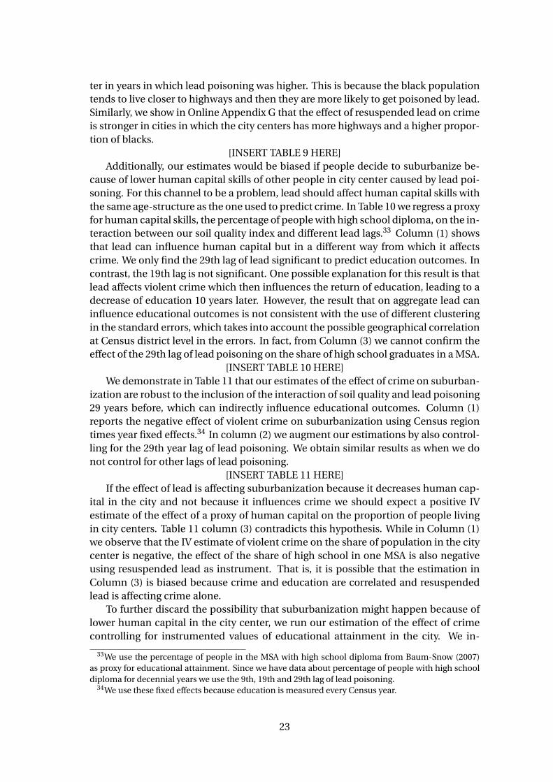
ter in years in which lead poisoning was higher. This is because the black populationtends to live closer to highways and then they are more likely to get poisoned by lead.Similarly, we show in Online Appendix G that the effect of resuspended lead on crimeis stronger in cities in which the city centers has more highways and a higher propor-tion of blacks.

[INSERT TABLE 9 HERE]Additionally, our estimates would be biased if people decide to suburbanize be-

cause of lower human capital skills of other people in city center caused by lead poi-soning. For this channel to be a problem, lead should affect human capital skills withthe same age-structure as the one used to predict crime. In Table 10 we regress a proxyfor human capital skills, the percentage of people with high school diploma, on the in-teraction between our soil quality index and different lead lags.33 Column (1) showsthat lead can influence human capital but in a different way from which it affectscrime. We only find the 29th lag of lead significant to predict education outcomes. Incontrast, the 19th lag is not significant. One possible explanation for this result is thatlead affects violent crime which then influences the return of education, leading to adecrease of education 10 years later. However, the result that on aggregate lead caninfluence educational outcomes is not consistent with the use of different clusteringin the standard errors, which takes into account the possible geographical correlationat Census district level in the errors. In fact, from Column (3) we cannot confirm theeffect of the 29th lag of lead poisoning on the share of high school graduates in a MSA.

[INSERT TABLE 10 HERE]We demonstrate in Table 11 that our estimates of the effect of crime on suburban-

ization are robust to the inclusion of the interaction of soil quality and lead poisoning29 years before, which can indirectly influence educational outcomes. Column (1)reports the negative effect of violent crime on suburbanization using Census regiontimes year fixed effects.34 In column (2) we augment our estimations by also control-ling for the 29th year lag of lead poisoning. We obtain similar results as when we donot control for other lags of lead poisoning.

[INSERT TABLE 11 HERE]If the effect of lead is affecting suburbanization because it decreases human cap-

ital in the city and not because it influences crime we should expect a positive IVestimate of the effect of a proxy of human capital on the proportion of people livingin city centers. Table 11 column (3) contradicts this hypothesis. While in Column (1)we observe that the IV estimate of violent crime on the share of population in the citycenter is negative, the effect of the share of high school in one MSA is also negativeusing resuspended lead as instrument. That is, it is possible that the estimation inColumn (3) is biased because crime and education are correlated and resuspendedlead is affecting crime alone.

To further discard the possibility that suburbanization might happen because oflower human capital in the city center, we run our estimation of the effect of crimecontrolling for instrumented values of educational attainment in the city. We in-

33We use the percentage of people in the MSA with high school diploma from Baum-Snow (2007)as proxy for educational attainment. Since we have data about percentage of people with high schooldiploma for decennial years we use the 9th, 19th and 29th lag of lead poisoning.

34We use these fixed effects because education is measured every Census year.

23

strument educational attainment using historic state compulsory education laws col-lected by Goldin and Katz (2008). In particular, we use two different measures of min-imum age of compulsory schooling in 1910 as instruments: the school entrance ageand the school leaving age. We obtain a time variant instrument for education bymultiplying minimum age of compulsory schooling by the U.S. proportion of peoplewith high school in a particular year. Results are reported in Table 12.

[INSERT TABLE 12 HERE]Columns (1) and (2) replicate our unconditional results. Columns (3) and (6) jointly

estimate the effect of violent crime and education on suburbanization using the twodifferent education instruments (columns (4)-(5) and (7)-(8) show the correspond-ing first stage regressions). Both column (3) and (6) show that the effect of crime onsuburbanization is robust to the inclusion of an instrumented education control.

7 Effect of crime on aggregate city variables

We have shown that violent crime has moved people and firms from city centers to thesuburbs. In this Section we explore whether this increase in violent crime and subur-banization has generated any aggregate effects on the city or if suburbanization is justa zero sum reshuffling of resources around the city. This is an important question totackle in order to gain understanding on how people and firms should be distributedin a city.

We first explore this question by looking at the effect that violent crime had onthe total population of the city, house prices and median income. Results in Table13 show that violent crime had no effect on city population while median incomeand house prices in the city increased. In fact, from Section 5.3 we already know thatviolent crime has only created movement of people inside the city and not betweencities. From Column (2) and (3) we can see that violent crime has a positive effecton MSA housing affordability both measured as median gross rent per housing unit(Column (2)) or median single family house value (Column (3)). Moreover, we findthat the increase in violent crimes is associated with higher income also controllingfor the education levels (Columns (4) and (5)).

[INSERT TABLE 13 HERE]In Table 14 we explore further what are the income effects of violent crime and if

violent crime generated any changes in the means of transportation used in a city. Weobserve, first of all, that while income increased overall in the city these gains have notenjoyed by people living in the city center. In fact, we observe that overall inequalitiesincrease in the city. In Column (1) we can observe that the Gini index within the cityincreased.

[INSERT TABLE 14 HERE]In Column (2) of Table 14 we can observe that the ratio between income in the city

center and the MSA decreased. In the city center the median income has decreasedbut not in a statistical significant way (Column (3)). On the other hand, the overallincome in the MSA has increased indicating that suburbs have become particularlyricher. This results are interesting because they uncover two dynamics that happenas a city becomes more violent and therefore suburbanized. The first is a selectionprocess, where richer individuals move to the suburbs leaving the poorest in the city

24

center. This is also in line with the results shown in Tables 5 and 8 on how the racialdistribution of people inside a city changes after an increase in violent crime.

The second can be understood in combination with the fact that the cities that arebecoming more violent and more suburbanized are not losing population. A way tomake this possible is that incomes in the MSA increase to compensate for the increasein violent crime, the increase in transportation cost, and other negative amenitiesthat the suburbanization process may generate. These two effects combined createthe observed changes in income after an increase in violent crime. In the city center,the two effects might go in opposite directions. Because of selection only the poor-est people stay but they have to be compensated with an increase in income so thatthey do not migrate to another city. The overall effect is that their income remainsunchanged. Instead in the suburbs the two effects might reinforce each other. Theincrease in violent crime moves the richest people to the suburbs and added to thisthey also need to be compensated for all the negative amenities.

It is important to notice that these results do not fit with a model in which violentcrime is only decreasing the amenities of a city. In that case, one would expect violentcrime to decrease the population and/or to decrease house prices. Another mecha-nism that can explain these results is that the increase in violent crime has generatedsome positive externality on productivity. In fact, we know from Table 6 that violentcrime increased employment decentralization, and city with multiple employmentcenters can be more productive.

Finally, we explore if violent crime generated also changes in the way that individ-uals move around the city. From Column (4) of Table 14 we can see that violent crimeboosts the construction of highways possibly to facilitate suburbanization of people.The construction of new infrastructure can potentially have effects on productivity ofthe city. Moreover, since we know from Baum-Snow (2007) that highways have a pos-itive effect on suburbanization, the effect of violent crime on suburbanization thatwe have found in Section 5.1 has to be interpreted as the general equilibrium effectof violent crime on suburbanization which do not partial out for the mediating factorof the highway construction. In column (5) we further observe that violent crime de-creases the use of public transportation. These two last results confirm the fact thatviolent crime generated suburbanization and this ultimately decreased the demandfor the use of public transportation and increased the demand for highways and theuse of car.

From the results of this Section we can speculate that amenities and productivityin the city might have been affected by the increase in violent crimes. In the nextSection we build a spatial equilibrium model in which every city is considered as adifferent economy in order to make sense of these between-cities comparisons andassess whether violent crime has influenced amenities and productivity.

7.1 Spatial equilibrium model

We rationalize the city-wide effects of violent crime using the Rosen-Roback spatialequilibrium model developed by Glaeser (2008) and Glaeser and Gottlieb (2009). Themodel has its base in the works of Rosen (1979) and Roback (1982), and the corner-stone of the model is the concept of spatial equilibrium: utility should be equalized

25

between people living in different spaces. The same model has been applied to studythe aggregate effect of city shape by Harari (2015). Each city (m) differs for its specificlevel of amenities (θm) and productivity (Am). We assume that violent crime has aneffect on these parameters. Our goal is to estimate how large and in which directionthe effect of violent crime on these parameters has to be to match the city-wide esti-mates. The model consists of three agents: workers, firms in production sector andfirms in construction sector.

Workers (i) have to decide in which city m to live. We assume perfect mobilitybetween cities. Moreover, they have to decide how much to consume of a consump-tion good (C) and housing (H). The price of the consumption good is normalized to1, while the price of housing is specified as p H

m . They supply inelastically labour andobtain a city-specific wage (wm). We assume a Cobb-Douglas utility function, whereα represents the share of housing into utility. If a city has a higher level of amenities(θm) workers receive higher utility from that. The problem of workers is therefore thefollowing one:

maxCi ,Hi

θmC 1−αi Hα

i

s.t. Ci = wm −p Hm Hi

The solution of the worker’s problem gives rise to the so-called spatial equilib-rium condition. Let’s define v̄m as the indirect utility that should be equalized be-tween cities. Plugging the optimal solution for the amount of housing, Hi = αwm

p Hm

, and

consumption good, Ci = (1−α) wm , into the utility and taking logs we can write thespatial equilibrium condition as in Equation 4. Lower amenities in one city shouldbe compensated by higher wages or lower house prices to obtain the same utility be-tween cities.

log (v̄m) = (1−α) log (1−α)+αl og (α)+ log (θm)+ log (wm)−αl og(p H

m

)(4)

The representative firm in production sector decides the amount of labour (N)and traded capital (K ) to hire to produce the consumption good. Labour is paid thewage level (wm). Traded capital can be purchased at a price of 1 in any location. Everycity is characterized by a specific level of productivity (Am) and a fixed-supply of non-traded capital (Z̄m). As reported in Glaeser (2008), the assumption of the existenceof traded and non-traded capital allows to have firms facing constant returns to scalebut to have decreasing returns to scale at city level, and then the presence of a finitenumber of firms in each city. We assume a Cobb-Douglas production function whereβ and γ represent the share of labour and traded capital into the production function.The problem of the firms in the production sector follows.

maxN ,K

Am NβK γZ̄ 1−β−γm −wm N −K

The solution of this problem gives rise to the labour demand condition reportedin logarithm terms in Equation 5.

l og (wm) = log(β)+ γ

1−γ log(γ)+ 1

1−γ log (Am)+ 1−β−γ1−γ

[log

(Z̄m

)− log(N̄

)](5)

26

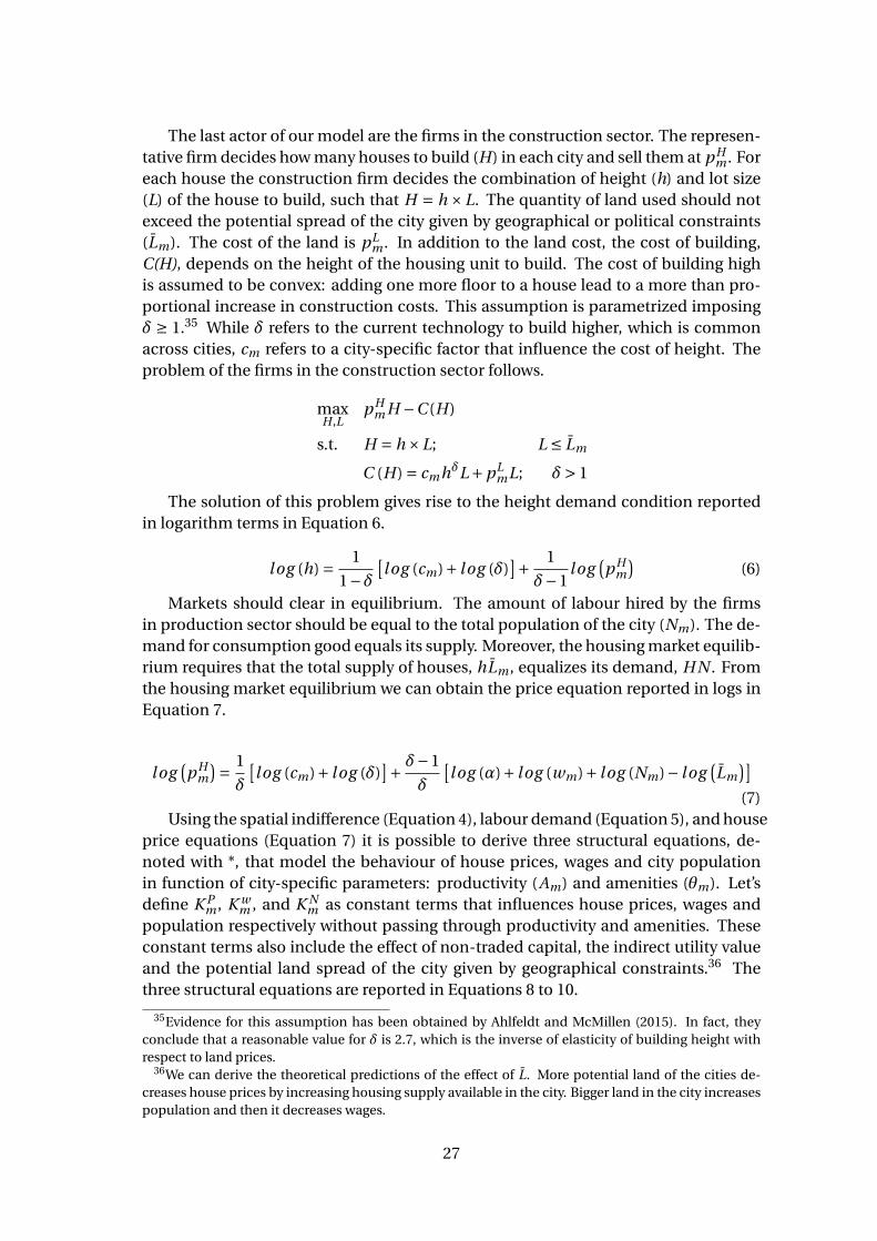
The last actor of our model are the firms in the construction sector. The represen-tative firm decides how many houses to build (H) in each city and sell them at p H

m . Foreach house the construction firm decides the combination of height (h) and lot size(L) of the house to build, such that H = h ×L. The quantity of land used should notexceed the potential spread of the city given by geographical or political constraints(L̄m). The cost of the land is pL

m . In addition to the land cost, the cost of building,C(H), depends on the height of the housing unit to build. The cost of building highis assumed to be convex: adding one more floor to a house lead to a more than pro-portional increase in construction costs. This assumption is parametrized imposingδ ≥ 1.35 While δ refers to the current technology to build higher, which is commonacross cities, cm refers to a city-specific factor that influence the cost of height. Theproblem of the firms in the construction sector follows.

maxH ,L

p Hm H −C (H)

s.t. H = h ×L; L ≤ L̄m

C (H) = cmhδL+pLmL; δ> 1

The solution of this problem gives rise to the height demand condition reportedin logarithm terms in Equation 6.

log (h) = 1

1−δ[log (cm)+ log (δ)

]+ 1

δ−1log

(p H

m

)(6)

Markets should clear in equilibrium. The amount of labour hired by the firmsin production sector should be equal to the total population of the city (Nm). The de-mand for consumption good equals its supply. Moreover, the housing market equilib-rium requires that the total supply of houses, hL̄m , equalizes its demand, H N . Fromthe housing market equilibrium we can obtain the price equation reported in logs inEquation 7.

log(p H

m

)= 1

δ

[log (cm)+ log (δ)

]+ δ−1

δ

[l og (α)+ log (wm)+ log (Nm)− log

(L̄m

)](7)

Using the spatial indifference (Equation 4), labour demand (Equation 5), and houseprice equations (Equation 7) it is possible to derive three structural equations, de-noted with *, that model the behaviour of house prices, wages and city populationin function of city-specific parameters: productivity (Am) and amenities (θm). Let’sdefine K P

m , K wm , and K N

m as constant terms that influences house prices, wages andpopulation respectively without passing through productivity and amenities. Theseconstant terms also include the effect of non-traded capital, the indirect utility valueand the potential land spread of the city given by geographical constraints.36 Thethree structural equations are reported in Equations 8 to 10.

35Evidence for this assumption has been obtained by Ahlfeldt and McMillen (2015). In fact, theyconclude that a reasonable value for δ is 2.7, which is the inverse of elasticity of building height withrespect to land prices.

36We can derive the theoretical predictions of the effect of L̄. More potential land of the cities de-creases house prices by increasing housing supply available in the city. Bigger land in the city increasespopulation and then it decreases wages.

27

log(p H∗

m

)= K Pm + (δ−1)

[log (Am)+βlog (θm)

]δ

(1−β−γ)+αβ (δ−1)

(8)

log(w∗

m

)= K wm + α (δ−1) log (Am)−δ(

1−β−γ)log (θm)

δ(1−β−γ)+αβ (δ−1)

(9)

log(N∗

m

)= K Nm + [δ−α (δ−1)] log (Am)+δ(

1−γ)log (θm)

δ(1−β−γ)+αβ (δ−1)

(10)

The theoretical predictions of our model are that house prices increases if a citybecomes more productive or increases its amenities. Wages are positively affected byproductivity. A decrease in amenities in the city should be compensated by higherwages in order to equalize utility at each location, ceteris paribus. Finally, city popu-lation increases city productivity and amenities.

We assume that violent crime (V C ccm ) can have externality effects on city produc-

tivity and amenities that are not taken into account by actors.37 We assume that theexogenous part of violent crime (V̂ C

ccm ) has a log-linear influence on these parame-

ters. We define λA and λθ as the reduced form elasticities of productivity and ameni-ties with respect to violent crime, respectively. We assume that city productivity andamenities are further influenced by constant terms (K A

m and K θm) and any other non-

constant factor not related to violent crime which composes errors (µAm and µθm).

log (Am) = K Am +λAlog

(V̂ C

ccm

)+µA

m (11)

log (θm) = K θm +λθlog

(V̂ C

ccm

)+µθm (12)

We are agnostic about the direction of the effects of violent crime on city-specificparameters. Violent crime can in principle decrease city amenities because peopleare not willing to live in a city with more crimes. Violent crimes can decrease produc-tivity by influencing human capital accumulation of the population.

Our objective is then to obtain the direction of the effects of violent crime on city-specific parameters that are in line with the estimated regressions of the city-wideeffects of violent crime on house prices, wages and city population using the strategyproposed by Glaeser (2008). In order to do this we substitute Equations 11 to 12 intothe structural equations (Equations 8 to 10) to obtain the reduced form equationsthat links violent crime to house prices, wages and city population (Equations 13 to15). As it is possible to see these equations do not depend anymore on productivityand amenities.

log(p∗H

m

)= K Pm +B P log

(V̂ C

ccm

)+µP

m (13)

log(w∗

m

)= K wm +B w l og

(V̂ C

ccm

)+µw

m (14)

37The model can be expanded to include the effect of violent crime on total land spread becausefor example it can influences zoning and regulation constraints. However, no result that we derivedepends on the assumption of no effect of violent crime on total land spread. This is similar to whathas been done in Harari (2015)

28

log(N∗

m

)= K Nm +B N log

(V̂ C

ccm

)+µN

m (15)

The reduced form elasticities of house prices, wages and city population with re-spect to violent crime (the B coefficients) are reported in Equations 16 to 18. Thesereduced forms coefficients depend on a set of parameters and on the reduced formelasticities of productivity and amenities with respect to violent crime (the λ param-eters). In particular, we have a set of three equations (B P , B w and B N ) and two un-knowns (λA and λθ). If we know the reduced form elasticities of house prices, wagesand city population with respect to violent crime we can potentially recover the re-duced form elasticities of productivity and amenities with respect to violent crime.

B P = (δ−1)λA +β (δ−1)λθ

αβ (δ−1)+δ(1−β−γ) (16)

B w = (δ−1)αλA −δ(1−β−γ)

λθ

αβ (δ−1)+δ(1−β−γ) (17)

B N = [δ (1−α)+α]λA +δ(1−γ)

λθ

αβ (δ−1)+δ(1−β−γ) (18)

The strategy proposed by Glaeser (2008) requires to first regress house prices, wagesand population of MSA on violent crime. In this way it is possible to estimate B̂ P , B̂ w ,and B̂ N , the reduced form elasticities of house prices, wages and city population withrespect to violent crime. In order to obtain the effect of the exogenous part of vio-lent crime on prices, wages and population we estimate Equations 13 to 15 using ourinstrumental variable strategy. Moreover, we proxy the constant terms (K P

m , K wm , and

K Nm ) by MSA and year fixed effects. The fixed spread of cities is captured by the MSA

fixed effects. Moreover, we have demonstrated in Section 4.4 that our instrument isnot related to the area of a city. Fixed effects at city level also captures non-tradedcapital. We also include Census Region time trends in our specification.38

Once we estimate B̂ P , B̂ w , and B̂ N we can recover the effect of violent crime onproductivity and amenities (λA and λθ) that rationalizes its city-wide effects usingEquations 19 and 20.

λA = (1−β−γ)

B̂ N + (1−γ)

B̂ w (19)

λθ =αB̂ P − B̂ w (20)

In our model we assume that agents are not heterogeneous. There exists an im-portant literature explaining why people sort in different locations based on on theirproductivity and valuation of amenities (see Combes et al., 2008). We do not suspectthat this important mechanism can bias our estimations since we have previouslydemonstrated that the change in violent crime did not alter the distribution of peoplebetween cities. Therefore, the estimated effects of violent crime on productivity andamenities can be interpreted as the effect which is not caused by sorting.

38Because we compare cities inside the same Census regions our assumption of perfect mobility ofpeople is more likely to be satisfied.

29

We assume some parameters in order to obtain the effect of violent crime on pro-ductivity and amenities. We approximate the share of housing in utility (α) by the totalconsumption expenditure to housing to be 0.3, obtained from the U.S. B.L.S. Con-sumption Expenditure Survey. As for Glaeser (2008), we assume the share of labourand traded capital in production function (β and γ) to be 0.6 and 0.3, respectively.

7.2 Estimating the externality effects

The strategy described in the previous section allows us to map reduced form elas-ticities of the effect of violent crime on observable variables, such as house prices,income and population in the MSA, on reduced form elasticities of the effect of vio-lent crime on unobservable variables, such as productivity and amenities. That is, wecan understand how violent crime might have changed these unobservable variablesin a way that is consistent with the model reported in the previous section.

The effect of violent crime on the observable variables is reported in Table 15.These results are slightly different from the results obtained in Section 7 because weneed to use a log-log specification in order to link these reduced forms to consider-ations about the externality effects of violent crime on productivity and amenities.However, we can still conclude that violent crime has a positive effect on city income,and house prices, leaving population unchanged.

[INSERT TABLE 15 HERE]Using Equations 19 to 20, we can recover how productivity and amenities should

have changed in order to rationalize the effect of violent crime on house prices, in-come and population in the MSA. The calculated externality effects of violent crimeon productivity and amenities (λA and λθ) are reported in Table 16, column (2).39 Wefind a negative and significant effect of violent crime on amenities (λθ) and a positiveeffect on productivity (λA), with an elasticity of -0.0991 and 0.1243 respectively. Usingthe theoretical predictions of our model if violent crime might affect amenities as aresult income should have increased as we found in Table 15. However, if amenitieswould have been the only city-specific factor changing this should have been reflectedin lower house prices, an effect that we do not observe. Therefore, productivity shouldhave necessarily increased as a result of higher violent crimes.

[INSERT TABLE 16 HERE]The estimates in Table 20 imply that the increase in violent crime in the city cen-

ter between 1960 and 1991 led to a decrease in the average amenities of the city of23.2%.40 Using equation 4 we can see that this quantity corresponds to the percent-age of the wage people would have been willing to sacrifice in 1991 to return to violentcrime rates in the city center as in 1960.

39Standard errors of the coefficients have been obtained using the following bootstrap technique.This strategy consists in first bootstrapping a panel sample from our distribution of observations; sub-sequently, we have estimated the elasticity of house prices, income and population to violent crimeand then compute the corresponding elasticity of amenities and productivity to violent crime; we havereplicated this procedure several times and obtained a distribution of these parameters and relevantstandard errors.

40Log violent crime in 1960 and 1991 was -7.08 and -4.73, respectively. We have computed the changein average amenities between 1960 and 1991 multiplying the elasticity of amenities to violent crime,-0.099, to the change in log violent crime in that period, 2.34.

30

We now explore if these effects are due directly because of the effect of violentcrime or by the effect of other variables that were affected by violent crime and ul-timately influenced productivity and amenities. In order to separate the real directeffect of violent crime on city-specific factors we control for several possible mediat-ing factors that we have found to be influenced by violent crime: highways, residentialsuburbanization and employment centralization. The results are reported in Table 16,columns (3) to (5), respectively. By controlling for these variables, we can partial outthe externality effect of violent crime which is not passing through these channels.

From Column (3) of Table 16 we can infer that, despite cities with more violentcrime lead to the creation of more highways, this last effect cannot explain why citieshave higher levels of productivity. The effect of violent crime on productivity which isnot passing through residential suburbanization is still positive, as it has been shownin Column (4) of Table 16. Moreover, controlling for the effect of violent crime on res-idential suburbanization we find a negative and stronger effect of violent crime oncity-amenities, with a calculated elasticity (λθ) of -0.1068. That is, if city centers in-crease their violent crimes and people cannot suburbanize then the impact of violentcrime on amenities is negative.

Finally, when we control for employment decentralization we do not find any ex-ternality effect of violent crime on unobservable variables (see Column (5) of Table16). The elasticity of violent crime on productivity (λA) is now not significant andequal to 0.1887. That is, the previous positive effect of violent crime on productivitycould be explained by the fact that violent crime led to a creation of different employ-ment centers in the city and this could boost firm productivity. This might mean thatsome firms were inefficiently located in the city center. Violent crime displaced firmsin the suburbs, and this displacement was productivity-enhancing. One possible ex-planation for this result is that historically it might have been more efficient to havefirms in the city center. Modern cities might have a different optimal distribution offirms in the city, for example as predicted by Lucas and Rossi-Hansberg (2002).41 Foran individual firm it might not be optimal to move outside the city center, despite thefact that productivity could increase if all firms coordinated this move outside of thecity center. Crime could have acted as a tax to firm location in city center that solvedthis coordination failure by making people and firms move.

The coefficient of the effect of violent crime on amenities also turns to be insignif-icant. The calculated elasticity of violent crime on amenities (λθ) is now -0.164. Thismight be explained by the fact that part of the decrease in amenities in the city is ex-plained by the fact that violent crime lead to employment to be located further awayfrom the center. As a result amenities could potentially decrease because of highertraffic and congestion externalities.

8 Concluding remarks

In this paper we provide evidence of a debated mechanism that can explain why U.S.cities suburbanized between the 1960s and the 1990s: the increase in violent crime in

41Lucas and Rossi-Hansberg (2002) predict that cities in equilibrium should have a business centerin the CBD, and further away: residential, business, mixed use, business, and residential areas respec-tively

31

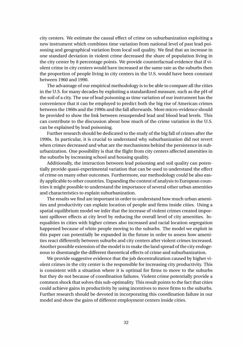
city centers. We estimate the causal effect of crime on suburbanization exploiting anew instrument which combines time variation from national level of past lead poi-soning and geographical variation from local soil quality. We find that an increase inone standard deviation in violent crime decreased the share of population living inthe city center by 8 percentage points. We provide counterfactual evidence that if vi-olent crime in city centers would have increased at the same rate as the suburbs thenthe proportion of people living in city centers in the U.S. would have been constantbetween 1960 and 1990.

The advantage of our empirical methodology is to be able to compare all the citiesin the U.S. for many decades by exploiting a standardized measure, such as the pH ofthe soil of a city. The use of lead poisoning as time variation of our instrument has theconvenience that it can be employed to predict both the big rise of American crimesbetween the 1960s and the 1990s and the fall afterwards. More micro-evidence shouldbe provided to show the link between resuspended lead and blood lead levels. Thiscan contribute to the discussion about how much of the crime variation in the U.S.can be explained by lead poisoning.

Further research should be dedicated to the study of the big fall of crimes after the1990s. In particular, it is crucial to understand why suburbanization did not revertwhen crimes decreased and what are the mechanisms behind the persistence in sub-urbanization. One possibility is that the flight from city centers affected amenities inthe suburbs by increasing school and housing quality.

Additionally, the interaction between lead poisoning and soil quality can poten-tially provide quasi-experimental variation that can be used to understand the effectof crime on many other outcomes. Furthermore, our methodology could be also eas-ily applicable to other countries. Expanding the context of analysis to European coun-tries it might possible to understand the importance of several other urban amenitiesand characteristics to explain suburbanization.

The results we find are important in order to understand how much urban ameni-ties and productivity can explain location of people and firms inside cities. Using aspatial equilibrium model we infer that the increase of violent crimes created impor-tant spillover effects at city level by reducing the overall level of city amenities. In-equalities in cities with higher crimes also increased and racial location segregationhappened because of white people moving to the suburbs. The model we exploit inthis paper can potentially be expanded in the future in order to assess how ameni-ties react differently between suburbs and city centers after violent crimes increased.Another possible extension of the model is to make the land spread of the city endoge-nous to disentangle the different theoretical effects of crime and suburbanization.

We provide suggestive evidence that the job decentralization caused by higher vi-olent crimes in the city center is the responsible for increasing city productivity. Thisis consistent with a situation where it is optimal for firms to move to the suburbsbut they do not because of coordination failures. Violent crime potentially provide acommon shock that solves this sub-optimality. This result points to the fact that citiescould achieve gains in productivity by using incentives to move firms to the suburbs.Further research should be devoted in incorporating this coordination failure in ourmodel and show the gains of different employment centers inside cities.

32

References

Ahlfeldt, G. M. and D. P. McMillen (2015). The vertical city: The price of land andthe height of buildings in chicago 1870-2010. Technical report, Spatial EconomicsResearch Centre, LSE.

Ahlfeldt, G. M., S. J. Redding, D. M. Sturm, and N. Wolf (2015). The economics ofdensity: Evidence from the berlin wall. Econometrica 83(6), 2127–2189.

Aizer, A. and J. Currie (2017). Lead and juvenile delinquency: New evidence fromlinked birth, school and juvenile detention records. Technical report, National Bu-reau of Economic Research.

Aizer, A., J. Currie, P. Simon, and P. Vivier (2016). Do low levels of blood lead reducechildren’s future test scores? Technical report, National Bureau of Economic Re-search.

Allen, T., C. Arkolakis, and X. Li (2015). Optimal city structure. Yale University, mimeo.Alonso, W. (1964). Location and land use. toward a general theory of land rent. Loca-

tion and land use. Toward a general theory of land rent..Angel, S., J. Parent, D. L. Civco, A. Blei, and D. Potere (2011). The dimensions of global

urban expansion: Estimates and projections for all countries, 2000–2050. Progressin Planning 75(2), 53–107.

Athey, S. and G. Imbens (2017). The state of applied econometrics: Causality andpolicy evaluation. Journal of Economic Perspective 31(2), 3–32.

Banks, E. C., L. E. Ferretti, and D. Shucard (1996). Effects of low level lead exposureon cognitive function in children: a review of behavioral, neuropsychological andbiological evidence. Neurotoxicology 18(1), 237–281.

Baum-Snow, N. (2007). Did highways cause suburbanization? The Quarterly Journalof Economics 122(2), 775–805.

Baum-Snow, N. and D. Hartley (2016). Accounting for Central Neighborhood Change,1980-2010. Working Paper Series WP-2016-9, Federal Reserve Bank of Chicago.

Baum-Snow, N. and B. F. Lutz (2011). School desegregation, school choice, andchanges in residential location patterns by race. The American economic re-view 101(7), 3019–3046.

Bianchi, M., P. Buonanno, and P. Pinotti (2012). Do immigrants cause crime? Journalof the European Economic Association 10(6), 1318–1347.

Billings, S. B. and K. T. Schnepel (2017, July). Life After Lead: Effects of Early Interven-tions for Children Exposed to Lead. IZA Discussion Papers 10872, Institute for theStudy of Labor (IZA).

Boustan, L. P. (2010). Was Postwar Suburbanization "White Flight"? Evidence fromthe Black Migration. The Quarterly Journal of Economics 125(1), 417–443.

Bowen, N. K. and G. L. Bowen (1999). Effects of crime and violence in neighborhoodsand schools on the school behavior and performance of adolescents. Journal ofAdolescent Research 14(3), 319–342.

Bradford, D. F. and H. H. Kelejian (1973). An econometric model of the flight to thesuburbs. Journal of Political Economy 81(3), 566–589.

Breiman, L., J. Friedman, C. J. Stone, and R. A. Olshen (1984). Classification and re-gression trees. CRC press.

33

Brueckner, J. K. and S. S. Rosenthal (2009). Gentrification and Neighborhood HousingCycles: Will America’s Future Downtowns Be Rich? The Review of Economics andStatistics 91(4), 725–743.

Canfield, R. L., C. R. Henderson Jr, D. A. Cory-Slechta, C. Cox, T. A. Jusko, and B. P. Lan-phear (2003). Intellectual impairment in children with blood lead concentrationsbelow 10 µg per deciliter. New England journal of medicine 348(16), 1517–1526.

Cecil, K. M., C. J. Brubaker, C. M. Adler, K. N. Dietrich, M. Altaye, J. C. Egelhoff, S. Wes-sel, I. Elangovan, R. Hornung, K. Jarvis, et al. (2008). Decreased brain volume inadults with childhood lead exposure. PLoS Med 5(5), e112.

Chalfin, A. and J. McCrary (2017). Criminal Deterrence : A Review of the Literature.Journal of Economic Literature 55(1).

Chandramouli, K., C. D. Steer, M. Ellis, and A. M. Emond (2009). Effects of early child-hood lead exposure on academic performance and behaviour of school age chil-dren. Archives of Disease in Childhood 94(11), 844–848.

Clark, H. F., D. J. Brabander, and R. M. Erdil (2006). Sources, sinks, and exposurepathways of lead in urban garden soil. Journal of Environmental Quality 35(6),2066–2074.

Clay, K., W. Troesken, and M. Haines (2014). Lead and mortality. Review of Economicsand Statistics 96(3), 458–470.

Combes, P.-P., G. Duranton, and L. Gobillon (2008). Spatial wage disparities: Sortingmatters! Journal of Urban Economics 63(2), 723–742.

Cullen, J. B. and S. D. Levitt (1999). Crime, Urban Flight, And The Consequences ForCities. The Review of Economics and Statistics 81(2), 159–169.

Daniele, V. and U. Marani (2011). Organized crime, the quality of local institutions andFDI in Italy: A panel data analysis. European Journal of Political Economy 27(1),132–142.

Dapul, H. and D. Laraque (2014). Lead poisoning in children. Advances in pedi-atrics 61(1), 313–333.

Denno, D. W. (1990). Biology and violence: From birth to adulthood. Cambridge Uni-versity Press.

Detotto, C. and E. Otranto (2010). Does crime affect economic growth? Kyklos 63(3),330–345.

Diamond, R. (2016). The determinants and welfare implications of us workers’ diverg-ing location choices by skill: 1980–2000. The American Economic Review 106(3),479–524.

Feigenbaum, J. J. and C. Muller (2016). Lead exposure and violent crime in the earlytwentieth century. Explorations in Economic History 62, 51–86.

Ferrie, J. P., K. Rolf, and W. Troesken (2012). Cognitive disparities, lead plumbing, andwater chemistry: Prior exposure to water-borne lead and intelligence test scoresamong world war two us army enlistees. Economics & Human Biology 10(1), 98–111.

Filippelli, G. M., M. A. Laidlaw, J. C. Latimer, and R. Raftis (2005). Urban lead poison-ing and medical geology: an unfinished story. GSA Today 15(1), 4–11.

Frey, W. H. (1979). Central city white flight: Racial and nonracial causes. AmericanSociological Review, 425–448.

34

Fujita, M. and H. Ogawa (1982). Multiple equilibria and structural transition of non-monocentric urban configurations. Regional science and urban economics 12(2),161–196.

Garcia-Lopez, M.-A., A. Holl, and E. Viladecans-Marsal (2015). Suburbanization andhighways in Spain when the Romans and the Bourbons still shape its cities. Journalof Urban Economics 85(C), 52–67.

Garcia-Lopez, M.-A., I. Pasidis, and E. Viladecans-Marsal (2015). Express delivery tothe suburbs? transportation effects in heterogeneous european cities.

Glaeser, E. L. (2008). Cities, Agglomeration and Spatial Equilibrium. New York: OxfordUniversity Press.

Glaeser, E. L. and J. D. Gottlieb (2009). The Wealth of Cities: Agglomeration Economiesand Spatial Equilibrium in the United States. Journal of Economic Literature 47(4),983–1028.

Glaeser, E. L. and M. E. Kahn (2001). Decentralized employment and the transforma-tion of the american city. Technical report, National Bureau of Economic Research.

Glaeser, E. L. and M. E. Kahn (2004). Sprawl and urban growth. Handbook of regionaland urban economics 4, 2481–2527.

Glaeser, E. L. and B. Sacerdote (1999). Why is there more crime in cities? Journal ofpolitical economy 107(S6), S225–S258.

Goldin, C. and L. F. Katz (2008). Mass secondary schooling and the state: the role ofstate compulsion in the high school movement. In Understanding long-run eco-nomic growth: Geography, institutions, and the knowledge economy, pp. 275–310.University of Chicago Press.

Goudriaan, H., K. Wittebrood, and P. Nieuwbeerta (2006). Neighbourhood character-istics and reporting crime: Effects of social cohesion, confidence in police effec-tiveness and socio-economic disadvantage. British Journal of Criminology 46(4),719–742.

Grönqvist, H., J. P. Nilsson, and P.-O. Robling (2016). Early lead exposure and out-comes in adulthood.

Grubb, W. N. (1982). The flight to the suburbs of population and employment, 1960–1970. Journal of Urban Economics 11(3), 348–367.

Harari, M. (2015). Cities in bad shape: Urban geometry in india. Job market paper,Massachusetts Institute of Technology.

Harnik, P., A. Martin, and K. Barnhart (2015). City park facts. Report. The Trust forPublic Land, Washington, DC, USA.

Henrich, C. C., M. Schwab-Stone, K. Fanti, S. M. Jones, and V. Ruchkin (2004). Theassociation of community violence exposure with middle-school achievement: Aprospective study. Journal of Applied Developmental Psychology 25(3), 327–348.

Hunt, A., D. L. Johnson, and D. A. Griffith (2006). Mass transfer of soil indoors bytrack-in on footwear. Science of the Total Environment 370(2), 360–371.

International Programme on Chemical Safety (1995). Environmental health criteria165: Inorganic lead. Technical report, World Health Organization Geneva.

Jargowsky, P. A. and Y. Park (2009). Cause or consequence? suburbanization and crimein us metropolitan areas. Crime & Delinquency 55(1), 28–50.

Kelly, M. (2000). Inequality and Crime. Review of Economics and Statistics 82(4), 530–539.

35

Kopecky, K. A. and R. M. Suen (2010). A quantitative analysis of suburbanization andthe diffusion of the automobile. International Economic Review 51(4), 1003–1037.

Laidlaw, M. A. and G. M. Filippelli (2008). Resuspension of urban soils as a persis-tent source of lead poisoning in children: a review and new directions. AppliedGeochemistry 23(8), 2021–2039.

Lucas, R. E. and E. Rossi-Hansberg (2002). On the internal structure of cities. Econo-metrica 70(4), 1445–1476.

Ludwig, J. (1998). Concealed-gun-carrying laws and violent crime: evidence fromstate panel data. International Review of Law and Economics 18(3), 239–254.

Mielke, H. (1999). Lead in the inner cities policies to reduce children’s exposure tolead may be overlooking a major source of lead in the environment. American sci-entist 87(1), 62–73.

Mieszkowski, P. and E. S. Mills (1993). The causes of metropolitan suburbanization.The Journal of Economic Perspectives 7(3), 135–147.

Mills, E. S. (1972). Studies in the structure of the urban economy.Mills, E. S. and L. S. Lubuele (1997). Inner cities. Journal of Economic Literature 35(2),

727–756.Moretti, E. (2011). Local labor markets. Handbook of labor economics 4, 1237–1313.Muth, R. (1969). Cities and housing: The spatial patterns of urban residential land

use. University of Chicago, Chicago.National Archive of Criminal Justice Data (2006). Law enforcement agency identifiers

crosswalk [united states], 2005 [computer file]. icpsr04634-v1.Needleman, H. L., C. McFarland, R. B. Ness, S. E. Fienberg, and M. J. Tobin (2002).

Bone lead levels in adjudicated delinquents: a case control study. Neurotoxicologyand teratology 24(6), 711–717.

Needleman, H. L., J. A. Riess, M. J. Tobin, G. E. Biesecker, and J. B. Greenhouse (1996).Bone lead levels and delinquent behavior. JAMA: The Journal of the American Med-ical Association 275(5), 363–369.

Nigg, J. T., M. Nikolas, G. Mark Knottnerus, K. Cavanagh, and K. Friderici(2010). Confirmation and extension of association of blood lead with attention-deficit/hyperactivity disorder (adhd) and adhd symptom domains at population-typical exposure levels. Journal of Child Psychology and Psychiatry 51(1), 58–65.

Nriagu, J. O. (1990). The rise and fall of leaded gasoline. Science of the total environ-ment 92, 13–28.

O’Flaherty, B. and R. Sethi (2015). Urban Crime, Volume 5 of Handbook of Regionaland Urban Economics, Chapter 0, pp. 1519–1621. Elsevier.

Patterson, C. C. (1965). Contaminated and natural lead environments of man.Archives of Environmental Health: An International Journal 11(3), 344–360.

Peryea, F. J. (2001). Gardening on lead-and arsenic-contaminated soils. WashingtonState University Cooperative Extension.

Rabin, R. (2008). The lead industry and lead water pipes "a modest campaign". Amer-ican journal of public health 98(9), 1584–1592.

Reber, S. J. (2005). Court Ordered Desegregation: Successes and Failures IntegratingAmerican Schools since Brown versus Board of Education. Journal of Human Re-sources 40(3).

36

Reddy, K. J., L. Wang, and S. P. Gloss (1995). Solubility and mobility of copper, zincand lead in acidic environments. Plant and Soil 171(1), 53–58.

Reyes, J. W. (2015a). Lead exposure and behavior: Effects on antisocial and risky be-havior among children and adolescents. Economic Inquiry 53(3), 1580–1605.

Reyes, J. W. (2015b). Lead policy and academic performance: Insights from mas-sachusetts. Harvard Educational Review 85(1).

Roback, J. (1982). Wages, rents, and the quality of life. The Journal of Political Econ-omy, 1257–1278.

Roper, W. L., V. Houk, H. Falk, and S. Binder (1991). Preventing lead poisoning inyoung children: A statement by the centers for disease control, october 1991. Tech-nical report, Centers for Disease Control, Atlanta, GA (United States).

Rosen, S. (1979). Wage-based indexes of urban quality of life. Current issues in urbaneconomics 3.

Rowe, D. C. (2002). Biology and crime. Roxbury Los Angeles, CA.Sampson, R. J. and A. S. Winter (2016). The racial ecology of lead poisoning: Toxic

inequality in chicago neighborhoods, 1995-2013. Du Bois Review: Social ScienceResearch on Race 13(2), 261–283.

Stehouwer, R. and K. Macneal (1999). Lead in residential soils: Sources, testing, andreducing exposure.

Stretesky, P. B. and M. J. Lynch (2001). The relationship between lead exposure andhomicide. Archives of pediatrics & adolescent medicine 155(5), 579–582.

Toscano, C. D. and T. R. Guilarte (2005). Lead neurotoxicity: from exposure to molec-ular effects. Brain Research Reviews 49(3), 529–554.

Traina, S. J. and V. Laperche (1999). Contaminant bioavailability in soils, sediments,and aquatic environments. Proceedings of the National Academy of Sciences 96(7),3365–3371.

Troesken, W. (2008). Lead water pipes and infant mortality at the turn of the twentiethcentury. Journal of Human Resources 43(3), 553–575.

United States Bureau of Mines, U. B. o. M. Minerals yearbook: Lead, 1941-1986.United States Department of Agriculture, Soil Survey Staff, N. R. C. S. Web soil survey.

http://websoilsurvey.nrcs.usda.gov/.United States Department of Justice, F. B. I. Uniform crime reporting program data

[united states]: Offenses known and clearances by arrest, 1960-2014.United States Department of Justice, F. B. I. (1993). Age-specific arrest rates and race-

specific arrest rates for selected offenses, 1965-1992.Wright, J. P., K. N. Dietrich, M. D. Ris, R. W. Hornung, S. D. Wessel, B. P. Lanphear,

M. Ho, and M. N. Rae (2008). Association of prenatal and childhood blood leadconcentrations with criminal arrests in early adulthood. PLoS Medicine 5(5), e101.

Zahran, S., M. A. Laidlaw, S. P. McElmurry, G. M. Filippelli, and M. Taylor (2013). Link-ing source and effect: Resuspended soil lead, air lead, and children’s blood leadlevels in detroit, michigan. Environmental science & technology 47(6), 2839–2845.

37

9 Figures and Tables

9.1 Figures

(a) Time series

(b) Scatter plot

Figure 1: Correlation between violent crime per capita and proportion of people living in thecity center

Panel a): Time series share population living in city center (CC), left y axis, and violent crime per capita in city center, right y axis. Panel b): Scatter plot change share

population living in city center (CC) between 1961 and 1991 against change violent crime per capita in city center.

38

Figure 2: Time series of violent crime rates per capita and the consumption of tetraethyl lead19 years before

Upward x axis: time series of tonnes of lead consumed in U.S. as gasoline additive. Downward x axis: time series of violent crime per capita in city center

Figure 3: Average marginal effect of tetraethyl lead at different pH values

Marginal effects derived after regressing violent crime per capita in city centers on tetraethyl lead, tetraethyl lead x pH, tetraethyl lead x pH2, and tetraethyl lead x pH3.

Robust standard errors have been used clustered at city level. Marginal effects reported for value of pH between the 10th and 99th percentile. p-value joint significance

polynomials: p-value for the test of joint significance of the coefficients of the following regressors: tetraethyl lead x pH, tetraethyl lead x pH2, and tetraethyl lead x pH3.

For every city center, we combine data for the average pH level from the United States Geological Survey with crime observations from F.B.I.

39

(a) Coefficients

(b) F-statistics

Figure 4: Coefficients and F-statistics of the first stage regression for every possible pH interval

Panel a): Coefficients of first stage regression. Panel b): F-statistics of first stage regression. Coefficient and F-statistic of the excluded instrument derived after regressing

violent crime per capita on city and year fixed effects and the interaction between tetraethyl lead 19 years before and the soil quality index. Every different circle refers to a

different regression for every possible minimum and maximum level of pH. Robust standard errors have been used. The size of the circles refer to the absolute value of the

coefficient or F-stat with respect to the coefficient or F-stat in the same category (- and sign.: negative and signficant, + and sign: positive and significant, n.s.: non

significant). Dashed lines indicate our chosen soil quality index: pH between 6.8 and 7.7

40

Figure 5: First stage using different lags of national lead poisoning

Left y axis: coefficient of the first stage estimate. Right y axis: F-statistics of the relevance of the instrument. For each possible lag of national lead (X), coefficient obtained

after regressing violent crime per capita in the city center on MSA, year and Census division times year fixed effects and the interaction between a dummy taking 1 if pH is

between 6.8 and 7.7 and the tonnes of lead consumed in U.S. as gasoline additive X years before, normalized by the maximum level of tetraethyl lead consumption.

F-statistics obtained as the F-statistics of the instrument in this regression.

Figure 6: Time series of violent crime per capita in city center by good and bad soil

City centers with good soil: pH between 6.8 and 7.7. City centers with bad soil: pH outside the interval between 6.8 and 7.7.

41

Figure 7: Map of city centers with good and bad soils for lead adsorption

City centers with good soil: pH between 6.8 and 7.7. City centers with bad soil: pH outside the interval between 6.8 and 7.7. The map reports the U.S. Census Divisions

Figure 8: Time series of the effect of the good soil index on crime and time series of laggedtetraethyl lead

Coefficients obtained regressing violent crime per capita on the interaction between the good soil dummy and year dummies, controlling for city, year and Census

division times year fixed effects. Standard errors have been clustered at Census Division level. Lower bound CI 10: lower bound confidence interval at 10 % significance

level. Higher bound CI 10: higher bound confidence interval at 10 % significance level. City centers with good soil: pH between 6.8 and 7.7. Lead: tonnes of lead

consumed in U.S. as gasoline additive 19 years before, normalized by the maximum level of tetraethyl lead consumption. 1960 year dummy has been omitted. Robust

standard errors have been used. Left y axis: effect of the good soil index on crime. Right y axis: time series of lagged tetraethyl lead.

42

Figure 9: Counterfactual proportion of people in city center in MSA if violent crime in citycenter would not have increased from 1960 and if violent crime in city center would haveincreased from 1960 as in the suburbs

Real: actual time series of proportion of people in city center in MSA. Counter. no incr in VC in CC: counterfactual proportion of people in city center in MSA if violent

crime (VC) in city center (CC) would not have increased from 1960 with corresponding 95 % confidence interval. Obtained subtracting the actual increase in violent crime

from one year in the city center to another multiplied by the causal effect of crime on suburbanization from the actual suburbanization measure. Counter. incr in VC as

NCC: counterfactual proportion of people in city center in MSA if violent crime in city center would have increased from 1960 as in the suburbs (NCC) with corresponding

95 % confidence interval. Obtained subtracting the actual difference in change in violent crime from one year to another in the city center with respect to the suburbs

multiplied by the causal effect of crime on suburbanization from the actual suburbanization measure. VC: Violent crime per capita. CC (NCC): city center (suburbs). l.b:

Lower bound confidence. u.b.: upper bound confidence.

43

9.2 Tables

Table 1: First stage using different fixed effects and time trends for all the years

(1) (2) (3) (4) (5)VARIABLES Violent crime Violent crime Violent crime Violent crime Violent crime

Good soil x Lead -0.00184*** -0.00528*** -0.00451*** -0.00327*** -0.00276***(0.000190) (0.000326) (0.000363) (0.000378) (0.000400)

Observations 9,515 9,515 9,484 9,484 9,363R-squared 0.005 0.757 0.763 0.771 0.832MSA FE NO YES YES YES YESYear FE NO YES YES YES YESC. reg X Year FE NO NO YES NO NOC. div X Year FE NO NO NO YES NOState X Year FE NO NO NO NO YESYear 60-91 60-91 60-91 60-91 60-91Estimation OLS OLS OLS OLS OLSF 262.16 154.46 74.80 47.78

For the notes see Table 2

Table 2: First stage using different fixed effects and time trends for Census Years

(1) (2) (3) (4) (5)VARIABLES Violent crime Violent crime Violent crime Violent crime Violent crime

Good soil x Lead -0.00206*** -0.00721*** -0.00556*** -0.00396*** -0.00325**(0.000611) (0.00120) (0.00134) (0.00140) (0.00145)

Observations 1,190 1,189 1,185 1,185 1,170R-squared 0.004 0.744 0.752 0.758 0.831MSA FE NO YES YES YES YESYear FE NO YES YES YES YESC. reg X Year FE NO NO YES NO NOC. div X Year FE NO NO NO YES NOState X Year FE NO NO NO NO YESYear CY 60-90 CY 60-90 CY 60-90 CY 60-90 CY 60-90Estimation OLS OLS OLS OLS OLSF 36.11 17.29 7.99 5.01

Violent crime: Violent crime per capita in the city center. Good soil x Lead: dummy taking 1 if pH in the city center is between 6.8 and 7.7 multiplied by tonnes of lead

consumed in U.S. as gasoline additive 19 years before, normalized by the maximum level of tetraethyl lead consumption. C. reg: Census region. C. div: Census division

fixed effects. CY: Census year. F: F-statistics on the excluded instrument. Robust standard errors have been used. Standard errors in parentheses. *** p<0.01, ** p<0.05, *

p<0.1

44

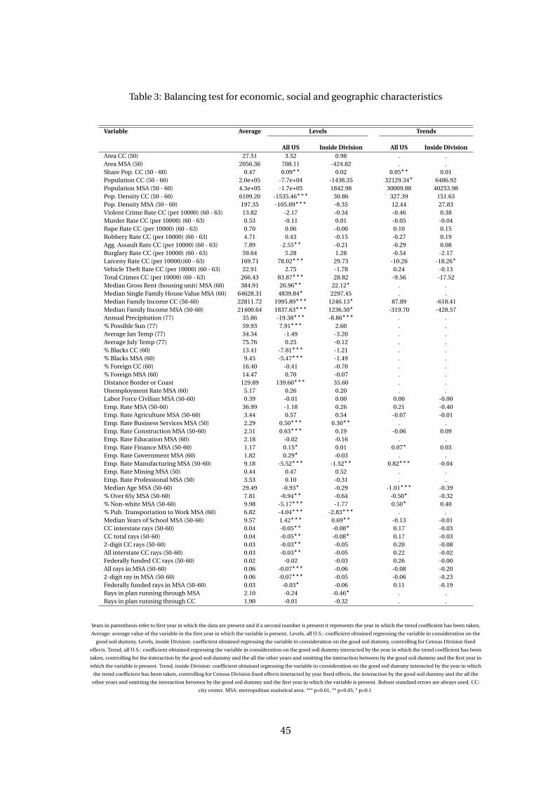
Table 3: Balancing test for economic, social and geographic characteristics

Variable Average Levels Trends

All US Inside Division All US Inside DivisionArea CC (50) 27.51 3.52 0.98 . .Area MSA (50) 2056.36 708.11 -424.82 . .Share Pop. CC (50 - 60) 0.47 0.09?? 0.02 0.05?? 0.01Population CC (50 - 60) 2.0e+05 -7.7e+04 -1438.35 32129.34? 6486.92Population MSA (50 - 60) 4.3e+05 -1.7e+05 1842.98 30009.88 40253.98Pop. Density CC (50 - 60) 6109.20 -1535.46??? 30.86 327.39 151.63Pop. Density MSA (50 - 60) 197.35 -105.09??? -8.35 12.44 27.83Violent Crime Rate CC (per 10000) (60 - 63) 13.82 -2.17 -0.34 -0.46 0.38Murder Rate CC (per 10000) (60 - 63) 0.53 -0.11 0.01 -0.05 -0.04Rape Rate CC (per 10000) (60 - 63) 0.70 0.06 -0.00 0.10 0.15Robbery Rate CC (per 10000) (60 - 63) 4.71 0.43 -0.15 -0.27 0.19Agg. Assault Rate CC (per 10000) (60 - 63) 7.89 -2.55?? -0.21 -0.29 0.08Burglary Rate CC (per 10000) (60 - 63) 59.64 5.28 1.28 -0.54 -2.17Larceny Rate CC (per 10000)(60 - 63) 169.71 78.02??? 29.73 -10.26 -18.26?

Vehicle Theft Rate CC (per 10000) (60 - 63) 22.91 2.75 -1.78 0.24 -0.13Total Crimes CC (per 10000) (60 - 63) 266.43 83.87??? 28.82 -9.56 -17.52Median Gross Rent (housing unit) MSA (60) 384.91 26.96?? 22.12? . .Median Single Family House Value MSA (60) 64628.31 4839.84? 2297.45 . .Median Family Income CC (50-60) 22811.72 1995.89??? 1246.13? 87.89 -618.41Median Family Income MSA (50-60) 21400.64 1837.63??? 1236.50? -319.70 -428.57Annual Precipitation (77) 35.86 -19.38??? -8.86??? . .% Possible Sun (77) 59.93 7.91??? 2.60 . .Average Jan Temp (77) 34.34 -1.49 -3.20 . .Average July Temp (77) 75.76 0.25 -0.12 . .% Blacks CC (60) 13.41 -7.81??? -1.21 . .% Blacks MSA (60) 9.45 -5.47??? -1.49 . .% Foreign CC (60) 16.40 -0.41 -0.70 . .% Foreign MSA (60) 14.47 0.70 -0.07 . .Distance Border or Coast 129.89 139.60??? 35.60 . .Unemployment Rate MSA (60) 5.17 0.26 0.20 . .Labor Force Civilian MSA (50-60) 0.39 -0.01 0.00 0.00 -0.00Emp. Rate MSA (50-60) 36.99 -1.18 0.26 0.21 -0.40Emp. Rate Agriculture MSA (50-60) 3.44 0.57 0.54 -0.07 -0.01Emp. Rate Business Services MSA (50) 2.29 0.50??? 0.30?? . .Emp. Rate Construction MSA (50-60) 2.51 0.63??? 0.19 -0.06 0.09Emp. Rate Education MSA (60) 2.18 -0.02 -0.16 . .Emp. Rate Finance MSA (50-60) 1.17 0.15? 0.01 0.07? 0.03Emp. Rate Government MSA (60) 1.82 0.29? -0.03 . .Emp. Rate Manufacturing MSA (50-60) 9.18 -5.52??? -1.52?? 0.82??? -0.04Emp. Rate Mining MSA (50) 0.44 0.47 0.52 . .Emp. Rate Professional MSA (50) 3.53 0.10 -0.31 . .Median Age MSA (50-60) 29.49 -0.93? -0.29 -1.01??? -0.39% Over 65y MSA (50-60) 7.81 -0.94?? -0.64 -0.50? -0.32% Non-white MSA (50-60) 9.98 -5.17??? -1.77 0.50? 0.40% Pub. Transportation to Work MSA (60) 6.82 -4.04??? -2.83??? . .Median Years of School MSA (50-60) 9.57 1.42??? 0.69?? -0.13 -0.01CC interstate rays (50-60) 0.04 -0.05?? -0.08? 0.17 -0.03CC total rays (50-60) 0.04 -0.05?? -0.08? 0.17 -0.032-digit CC rays (50-60) 0.03 -0.03?? -0.05 0.20 -0.08All interstate CC rays (50-60) 0.03 -0.03?? -0.05 0.22 -0.02Federally funded CC rays (50-60) 0.02 -0.02 -0.03 0.26 -0.00All rays in MSA (50-60) 0.06 -0.07??? -0.06 -0.08 -0.202-digit ray in MSA (50-60) 0.06 -0.07??? -0.05 -0.06 -0.23Federally funded rays in MSA (50-60) 0.03 -0.03? -0.06 0.11 -0.19Rays in plan running through MSA 2.10 -0.24 -0.46? . .Rays in plan running through CC 1.90 -0.01 -0.32 . .

Years in parenthesis refer to first year in which the data are present and if a second number is present it represents the year in which the trend coefficient has been taken.

Average: average value of the variable in the first year in which the variable is present. Levels, all U.S.: coefficient obtained regressing the variable in consideration on the

good soil dummy. Levels, inside Division: coefficient obtained regressing the variable in consideration on the good soil dummy, controlling for Census Division fixed

effects. Trend, all U.S.: coefficient obtained regressing the variable in consideration on the good soil dummy interacted by the year in which the trend coefficient has been

taken, controlling for the interaction by the good soil dummy and the all the other years and omitting the interaction between by the good soil dummy and the first year in

which the variable is present. Trend, inside Division: coefficient obtained regressing the variable in consideration on the good soil dummy interacted by the year in which

the trend coefficient has been taken, controlling for Census Division fixed effects interacted by year fixed effects, the interaction by the good soil dummy and the all the

other years and omitting the interaction between by the good soil dummy and the first year in which the variable is present. Robust standard errors are always used. CC:

city center. MSA: metropolitan statistical area. *** p<0.01, ** p<0.05, * p<0.1

45

Table 4: Baseline results: The effect of crime on suburbanization

(1) (2) (3) (4) (5) (6)VARIABLES Share Pop CC Violent crime Share Pop CC Share Pop CC Share Pop CC ln(Pop CC)

Violent crime -0.0165*** -0.0717*** -0.0843*** -0.257***(0.00141) (0.0121) (0.0167) (0.0718)

Good soil x Lead -0.914*** 0.0686***(0.0649) (0.00885)

Observations 9,481 9,484 9,481 9,716 9,481 9,484R-squared 0.960 0.758 0.956 0.934MSA FE YES YES YES YES YES YESYear FE YES YES YES YES YES YESC. div x Year NO NO NO NO YES YESYear 60-91 60-91 60-91 60-91 60-91 60-91Estimation OLS OLS IV OLS IV IVF . . 264.55 . 77.32 76.96

Share Pop CC: Proportion of MSA population living in city center. Violent crime: Violent crime per capita in the city center

standardized. Good soil x Lead: dummy taking 1 if pH in the city center is between 6.8 and 7.7 multiplied by tonnes of lead

consumed in U.S. as gasoline additive 19 years before, normalized by the maximum level of tetraethyl lead consumption. C.

div: Census Division fixed effects. F: Cragg-Donald Wald F-statistics on the excluded instruments. Standard errors clustered at

Census division times year level in parentheses. *** p<0.01, ** p<0.05, * p<0.1

Table 5: The effect of crime on population displacement

(1) (2) (3) (4) (5)VARIABLES Log Pop MSA Log Pop CC Log Pop NCC Blacks MSA Blacks CC

Violent crime 0.0661 -0.257*** 0.144*** 0.137 4.730***(0.0428) (0.0718) (0.0534) (0.809) (0.795)

Observations 9,481 9,484 9,481 921 916MSA FE YES YES YES YES YESYear FE YES YES YES YES YESC. div x Year YES YES YES NO NOC. reg x Year NO NO NO YES YESYear 60-91 60-91 60-91 CY 60-90 CY 60-90Estimation IV IV IV IV IVF 77.06 76.96 77.06 13.29 12.78

Violent crime: Violent crime per capita in the city center standardized. Pop MSA: Population in the MSA. Pop CC: Population in

the city center. Pop NCC: Population in the suburbs. C. div: Census Division fixed effects. C. reg: Census Region fixed effects. F:

Cragg-Donald Wald F-statistics on the excluded instruments. Standard errors clustered at Census division times year level

(columns 1-3) and Census region times year level (columns 4-5) in parentheses. *** p<0.01, ** p<0.05, * p<0.1

46

Table 6: The effect of crime on proportion of MSA employment in central city county

(1) (2) (3) (4) (5) (6)VARIABLES All Manuf Wholesale Retail Finance Other serv

Violent crime -0.0108 -0.0462*** -0.0244* -0.0386*** 0.00283 -0.0285***(0.0113) (0.0163) (0.0143) (0.0148) (0.0178) (0.0103)

Observations 5,334 5,334 5,334 5,334 5,334 5,334MSA FE YES YES YES YES YES YESYear FE YES YES YES YES YES YESC. div x Year YES YES YES YES YES YESYear 74-91 74-91 74-91 74-91 74-91 74-91Estimation IV IV IV IV IV IVF 19.37 19.37 19.37 19.37 19.37 19.37

Violent crime: Violent crime per capita in the city center standardized. Dependent variable is proportion of MSA employment

of SIC industry under consideration in county of the city center. All: all SIC employment. Manuf: Manufacturing; Wholesale:

Wholesale Trade; Retail: Retail Trade; Finance: Finance, Insurance, And Real Estate; Other serv: Services). MSA with a unique

county have missing values of employment proportion. C. div: Census Division fixed effects. F: Cragg-Donald Wald F-statistics

on the excluded instruments. Standard errors clustered at Census division times year level in parentheses. *** p<0.01, ** p<0.05,

* p<0.1

Table 7: Timing of residential and employment decentralization

(1) (2) (3) (4)VARIABLES Share Manuf CC Share Manuf CC Share Pop CC Share Pop CC

Violent crime -0.0241*** -0.0181 -0.0276*** -0.0478***(0.00863) (0.0187) (0.00631) (0.0127)

Share Pop CC (10 years lag) 0.0656***(0.0241)

Share Manuf CC (10 years lag) 0.0256(0.0185)

Observations 5,352 5,332 5,367 2,344MSA FE YES YES YES YESYear FE YES YES YES YESGood Soil x Lead 29 years lag NO YES NO YESYear 74-91 74-91 74-91 74-91Estimation IV IV IV IVF 74.24 15.32 76.87 19.57

Violent crime: Violent crime per capita in the city center standardized. Share Pop CC: Proportion of MSA population living in

city center.Share Manuf CC: proportion of MSA employment of manufacturing industry under consideration in county of the

city center. MSA with a unique county have missing values of employment proportion. F: Cragg-Donald Wald F-statistics on

the excluded instruments. Robust standard errors in parentheses. *** p<0.01, ** p<0.05, * p<0.1

47

Table 8: Profile of recent suburbanized population in 1980

Variable Recent suburbanized Difference wrt people staying in CCMean age 31.03 -2.86???

Mean number children 0.67 0.10???

Prop. married 0.62 0.09???

Prop. white 0.85 0.16???

Prop. black 0.11 -0.15???

Prop. high school or higher 0.63 0.14???

Prop. high school or higher of whites 0.64 0.11???

Prop. employed 0.55 0.11???

Prop. unemployed 0.03 -0.00???

Prop. people not working in CC 0.24 0.21???

Mean occupational score 18.69 4.18???

Prop.: Proportion. Recent suburbanized refers to people who in 1980 lives in a not central city in the metropolitan area and in the previous five years they were living in

the central city of the same metropolitan area. Difference with respect to people staying in CC has been obtained regressing the variable under interested on a variable

indicating whether the person is a recent suburbanized or he continues to live in the central city for the sample of people living in metropolitan areas. *** p<0.01, **

p<0.05, * p<0.1

Table 9: Heterogeneous effects of correlation between crime rates and proportion blacks liv-ing in city center

(1)VARIABLES Violent crime

Prop. Blacks CC 0.000379***(8.11e-05)

Prop. Blacks CC x Rays CC -3.10e-05**(1.10e-05)

Prop. Blacks CC x Rays CC x Lead 4.90e-05***(9.02e-06)

Observations 916R-squared 0.798MSA FE YESYear FE YESC. reg X Year FE YESYear CY 60-90Estimation OLS

Violent crime: Violent crime per capita in the city center. Prop. Blacks CC: proportion of black population in city center in the MSA. Rays CC: number of highway rays

passing through the city center, source: Baum-Snow (2007). Lead: tonnes of lead consumed in U.S. as gasoline additive 19 years before, normalized by the maximum level

of tetraethyl lead consumption. C. reg: Census region fixed effects. CY: census years. Standard errors clustered at Census region times year level in parentheses. *** p<0.01,

** p<0.05, * p<0.1

48

Table 10: Effect of interaction good soil and different lag of past leads on education outcomesand crime

(1) (2)VARIABLES Share high school Share high school

Good soil x Lead (9 years before) -0.546 -0.546(0.708) (1.860)

Good soil x Lead (19 years before) 0.699 0.699(1.895) (4.270)

Good soil x Lead (29 years before) -9.485*** -9.485(2.132) (5.846)

Observations 1,174 1,174R-squared 0.979 0.979MSA FE YES YESYear FE YES YESC. reg x Year YES YESYear CY 60-90 CY 60-90Estimation OLS OLSs.e. cluster MSA C. reg x Year

Violent crime: Violent crime per capita in the city center. Share high school: share of population with high school diploma in the MSA. Good soil x Lead (X years before):

dummy taking 1 if pH in the city center is between 6.8 and 7.7 multiplied by tonnes of lead consumed in U.S. as gasoline additive X years before, normalized by the

maximum level of tetraethyl lead consumption. CY: Census years. C. reg: Census region fixed effects. CY: census years. s.e. cluster: cluster level of the standard errors.

Standard errors in parentheses. *** p<0.01, ** p<0.05, * p<0.1

Table 11: Results controlling for different lagged effect of education level

(1) (2) (3)VARIABLES Share pop CC Share pop CC Share pop CC

Violent crime -0.0591*** -0.0781***(0.00678) (0.0289)

Good soil x Lead (29 years before) -0.0166(0.0208)

Share high school MSA -0.0105**(0.00426)

Observations 9,481 9,481 939MSA FE YES YES YESYear FE YES YES YESC. reg x Year FE YES YES YESYear 60-91 60-91 CY 60-90Estimation IV IV IVF 156.25 5.52 50.54

For the notes see Table 12. Robust standard errors in parentheses. *** p<0.01, ** p<0.05, * p<0.1

49

Table 12: Results controlling for instrumented education level

(1) (2) (3) (4) (5) (6) (7) (8)VARIABLES Sh. pop CC V. crime Sh. pop CC H.s. MSA V. crime Sh. pop CC H.s. MSA V. crime

Violent crime -0.0686*** -0.0611*** -0.0827***(0.0214) (0.0120) (0.0232)

Share high school MSA -0.00183 0.000998(0.00198) (0.00245)

Good soil x Lead -0.957*** -7.135*** -1.024*** -7.008*** -1.018***(0.192) (1.906) (0.211) (1.964) (0.213)

H.s. U.S. x age school entry 0.0131*** -0.00259**(0.00164) (0.000899)

H.s. U.S. x age school leave 0.00713*** -0.000962*(0.00116) (0.000544)

Observations 1,184 1,185 917 935 1,181 917 935 1,181MSA FE YES YES YES YES YES YES YES YESYear FE YES YES YES YES YES YES YES YESC. reg x Year FE YES YES YES YES YES YES YES YESYear CY 60-90 CY 60-90 CY 60-90 CY 60-90 CY 60-90 CY 60-90 CY 60-90 CY 60-90Estimation IV OLS IV OLS OLS IV OLS OLSF 17.51 . 12.24 . . 7.97 . .

Sh pop CC: Proportion of MSA population living in city center. V. crime: Violent crime per capita in the city center standardized.Good soil x Lead: dummy taking 1 if pH in the city center is between 6.8 and 7.7 multiplied by tonnes of lead consumed in U.S.as gasoline additive 19 years before, normalized by the maximum level of tetraethyl lead consumption. Share high school MSA:Percentage of people with high school diploma in the MSA. H.s. U.S.: Percentage of people with high school diploma in the U.S.

Age school entry: state age school of entry in 1910. Age school leave: State minimum age school leave in 1910. C. reg: CensusRegion fixed effects. CY: Census Year. F: F-statistics on the excluded instruments. Stock-Yogo weak ID test critical value at 10%maximal IV size: 7.03. Standard errors clustered at Census region times year level in parentheses. *** p<0.01, ** p<0.05, * p<0.1

Table 13: Effect of violent crime on MSA population, house prices, and income

(1) (2) (3) (4) (5)VARIABLES Pop. MSA H. rent MSA H. price MSA Inc MSA Inc MSA

Violent crime 95,144 57.94*** 21,690** 3,422** 836.2*(68,244) (16.58) (8,838) (1,252) (449.5)

Observations 921 921 920 921 917MSA FE YES YES YES YES YESYear FE YES YES YES YES YESC. reg x Year YES YES YES YES YESYear CY 60-90 CY 60-90 CY 60-90 CY 60-90 CY 60-90Controls . . . . EducationEstimation IV IV IV IV IVF 13.29 13.29 13.41 13.29 12.24

Violent crime: Violent crime per capita in the city center standardized. Pop MSA: Population in the MSA. H. rent MSA: Median

gross rent per housing unit in the MSA. H. price MSA: Median single family house value. Inc MSA: Median family income in the

MSA. Control for education: control for the percentage of people with high school diploma in the MSA instrumented by the

state age school of entry in 1910 multiplied by the overall percentage of people with high school diploma in the U.S. CY: Census

years. C. reg: Census Region fixed effects. F: F-statistics on the excluded instruments. Standard errors clustered at Census

region times year level in parentheses. *** p<0.01, ** p<0.05, * p<0.1

50

Table 14: Effect of violent crime on MSA inequalities and transportation

(1) (2) (3) (4) (5)VARIABLES Gini MSA Inc CC/MSA Inc CC Highway CC Pub transp MSA

Violent crime 0.00613** -0.0945*** -358.3 0.255* -2.212**(0.00243) (0.0210) (1,394) (0.135) (0.946)

Observations 921 921 921 921 921MSA FE YES YES YES YES YESYear FE YES YES YES YES YESC. reg x Year YES YES YES YES YESYear CY 60-90 CY 60-90 CY 60-90 CY 60-90 CY 60-90Estimation IV IV IV IV IVF 13.29 13.29 13.29 13.29 13.29

Violent crime: Violent crime per capita in the city center standardized. Inc CC/MSA: ratio between the median family income

in the city center (CC) and the median family income in the MSA. Inc CC: median family income in the city center. Gini MSA:

Simulated Gini coefficient from Baum-Snow (2007). Pub trans MSA: percentage of people using public transport to get to work.

Highway CC: highway rays built passing through city center. CY: Census years. C. reg: Census Region fixed effects. F: F-statistics

on the excluded instruments. Standard errors clustered at Census region times year level in parentheses. *** p<0.01, ** p<0.05, *

p<0.1

Table 15: Elasticities of house rents, income and population with respect to violent crime

(1) (2) (3)VARIABLES Log h. rent MSA Log income MSA Log Pop. MSA

Log violent crime 0.193** 0.157* 0.145(0.0836) (0.0880) (0.141)

Observations 918 918 918R-squared 0.830 0.838 0.990MSA FE YES YES YESYear FE YES YES YESC. reg x Year YES YES YESYear CY 60-90 CY 60-90 CY 60-90Estimation IV IV IVCluster s.e. MSA MSA MSAF 11.69 11.69 11.69

H. rent MSA: Median gross rent per housing unit in the MSA. Income MSA: Median family income in the MSA. Pop. MSA: Total

population in the MSA. Violent crime: Violent crime per capita in the city center standardized. C. reg: Census Region fixed

effects. CY: Census Year. F: F-statistics on the excluded instruments. Standard errors clustered at Census region times year level

in parentheses. *** p<0.01, ** p<0.05, * p<0.1

51

Table 16: Elasticities of amenities and productivity with respect to violent crime

Control for mediationCoefficient None Highways Resid suburbanization Empl centralization

λθ -0.0991** -0.0972** -0.1068** -0.164(0.04551) (0.04371) (0.04552) (0.6082)

λA 0.1243** 0.1219** 0.1260** 0.1887(0.05242) (0.04991) (0.05111) (0.62977)

λθ : elasticity of city amenities with respect to violent crime. λA : elasticity of city productivity with respect to violent crime.

Control for mediation, highways: the estimated regression also includes the number of highways passing through the MSA.

Control for mediation, resid suburbanization: the estimated regression also includes the proportion of population in MSA

living in city center. Control for mediation, empl centralization: the estimated regression also includes the proportion of

employment in MSA located in the central county. Standard errors have been bootstrapped: this strategy consists in first

bootstrapping a panel sample from our distribution of observations; subsequently, we have estimated the elasticity of house

prices, income and population to violent crime and then compute the corresponding elasticity of amenities and productivity to

violent crime; we have replicated this procedure several times and obtained a distribution of these parameters and relevant

standard errors. Standard errors in parentheses. *** p<0.01, ** p<0.05, * p<0.1

52