MULTILEVEL MONTE CARLO FINITE VOLUME METHODS FOR …klingen/e... · Resume 1991 Mathematics Subject...
20
Mathematical Modelling and Numerical Analysis Will be set by the publisher Mod´ elisation Math´ ematique et Analyse Num´ erique MULTILEVEL MONTE CARLO FINITE VOLUME METHODS FOR RANDOM CONSERVATION LAWS WITH DISCONTINUOUS FLUX Jayesh Badwaik 1 , Nils Henrik Risebro 2 and Christian Klingenberg 1 Abstract. We consider a random scalar hyperbolic conservation law in one spatial dimension with bounded random flux functions which are discontinuous in the spatial variable. We show that there exists a unique random entropy solution to the conservation law for corresponding to the specific entropy condition used to solve the deterministic case. Using the empirical convergence rates of the underlying deterministic problem over a broad range of parameters, we present a convergence analysis of a multilevel Monte Carlo Finite Volume Method (MLMC-FVM). It is based on a pathwise application of the finite volume method for the deterministic conservation laws. We show that the work required to compute the MLMC-FVM solutions is an order lower than the work required to compute the Monte Carlo Finite Volume Method solutions with equal accuracy. R´ esum´ e. Resume 1991 Mathematics Subject Classification. 65U05,35L65. The dates will be set by the publisher. 1. Introduction One dimensional scalar conservation laws with discontinuous flux in the space variables are often used to model different phenomena such as traffic flow [12, 22, 28], two phase flow in a porous media [?, 10, 11, 13–15] and sedimentation processes [5, 6, 9]. In one space dimension, a Cauchy problem for the model typically looks like ∂u ∂t + ∂ f ( k,u ) ∂x =0 x ∈ R,t> 0 (1a) u(x, 0) = u 0 (x) (1b) where k(x) is allowed to be discontinuous in x. Here u(x, t) is the unknown function while k(x) and the Cauchy data u 0 (x) are assumed to be known. Even for a differentiable k(x) and smooth initial conditions, the solutions are generally discontinuous. Hence, we consider the weak form of the equations. Weak solutions are non-unique, and we require admissibility conditions to select a unique solution. In the case of a differentiable k(x), admissibility conditions guaranteeing uniqueness of solutions are well known [4, 8, 16]. Keywords and phrases: Uncertainty Quantification, Conservation Law, Numerical Methods 1 University of W¨ urzburg 2 University of Oslo c EDP Sciences, SMAI 1999
Transcript of MULTILEVEL MONTE CARLO FINITE VOLUME METHODS FOR …klingen/e... · Resume 1991 Mathematics Subject...

Mathematical Modelling and Numerical Analysis Will be set by the publisher
Modelisation Mathematique et Analyse Numerique
MULTILEVEL MONTE CARLO FINITE VOLUME METHODS FOR RANDOM
CONSERVATION LAWS WITH DISCONTINUOUS FLUX
Jayesh Badwaik1, Nils Henrik Risebro2 and Christian Klingenberg1
Abstract. We consider a random scalar hyperbolic conservation law in one spatial dimension withbounded random flux functions which are discontinuous in the spatial variable. We show that thereexists a unique random entropy solution to the conservation law for corresponding to the specificentropy condition used to solve the deterministic case. Using the empirical convergence rates of theunderlying deterministic problem over a broad range of parameters, we present a convergence analysisof a multilevel Monte Carlo Finite Volume Method (MLMC-FVM). It is based on a pathwise applicationof the finite volume method for the deterministic conservation laws. We show that the work requiredto compute the MLMC-FVM solutions is an order lower than the work required to compute the MonteCarlo Finite Volume Method solutions with equal accuracy.
Resume. Resume
1991 Mathematics Subject Classification. 65U05,35L65.
The dates will be set by the publisher.
1. Introduction
One dimensional scalar conservation laws with discontinuous flux in the space variables are often used tomodel different phenomena such as traffic flow [12, 22, 28], two phase flow in a porous media [?, 10, 11, 13–15]and sedimentation processes [5, 6, 9]. In one space dimension, a Cauchy problem for the model typically lookslike
∂u
∂t+∂f(k, u)
∂x= 0 x ∈ R, t > 0 (1a)
u(x, 0) = u0(x) (1b)
where k(x) is allowed to be discontinuous in x. Here u(x, t) is the unknown function while k(x) and the Cauchydata u0(x) are assumed to be known.
Even for a differentiable k(x) and smooth initial conditions, the solutions are generally discontinuous. Hence,we consider the weak form of the equations. Weak solutions are non-unique, and we require admissibilityconditions to select a unique solution. In the case of a differentiable k(x), admissibility conditions guaranteeinguniqueness of solutions are well known [4,8, 16].
Keywords and phrases: Uncertainty Quantification, Conservation Law, Numerical Methods
1 University of Wurzburg2 University of Oslo
c© EDP Sciences, SMAI 1999
2 TITLE WILL BE SET BY THE PUBLISHER
For a discontinuous flux, the equation (1) has been studied extensively by [3,17,29] and different admissibilityconditions have been developed to select a unique solution. However, the different conditions, though yieldinguniqueness, give different unique solutions. Finite volume methods for (1) have been developed in [17,29]. Thestability of solutions with respect to the Cauchy data was examined and shown in [18].
However, often Cauchy data is not known exactly [21] and is only given with via certain statistical quantitiesof interest like mean, variances and higher moments. The uncertainty in the Cauchy data is carried over to theuncertainty in the solution of the equation. Uncertainty in the Cauchy data and the corresponding solutionis frequently modeled in a probabilistic manner. Here, we take the point of view that the Cauchy Data is arandom variable described by a probability distribution. Furthermore, we adopt a simplification of the problem,wherein the flux function f is of the multiplicative form f(k, u) = k(x)f(u). The equation then reads
∂u
∂t+∂(k(ω;x)f(u)
)∂x
= 0 x ∈ R, t > 0 (2a)
u(ω;x, 0) = u0(ω;x) (2b)
where k(ω; ·) and u0(ω, ·) are some functions from a probability space Ω into some relevant function space.Development of efficient algorithms to quantify the uncertainty in the solutions of random conservation law
is an active field of research. The challenge is to efficiently resolve the discontinuities that propagate from thephysical space to the probability space in a robust manner. Also, the number of random sources driving theuncertainty may be very large, and possibly countably infinite as well. The numerical method should be ableto deal with the corresponding possibly infinite dimensional spaces efficiently.
There are different methods to quantify the uncertainty in solutions of conservation laws, namely stochasticGalerkin method [1, 7, 23, 27, 31] based on generalized polynomial chaos, stochastic collocation [24, 32] andstatistical sampling methods, especially Monte Carlo (MC) methods [25]. As was shown in [26], the MCmethods converge to the mean at rate 1/2 as the number of samples M increase. This rate is due to the centrallimit theorem and hence, is optimal for these class of methods. This makes the MC methods computationallyexpensive.
In order to address this drawback, a multilevel Monte Carlo (MLMC) algorithm was proposed in [25] for arandom initial condition u0 and flux of the form f = f(u) with differentiable f . Later, for the case of uncertaintyin a smooth flux, a Multilevel Monte Carlo method was developed in [26]. A optimized combination of samplingsizes for different levels of spatial and temporal resolution were developed in the same paper to achieve themaximum accuracy in the statistical estimates of the first and higher order moments of the random solution.This analysis was vitally based on error analysis of the random conservation law.
Contrastingly, for the problems with discontinuous flux, Adimurthi et. al. [2] have demonstrated an examplewhere the total variation of the solution is unbounded near the discontinuous interface. This precludes a deter-mination of convergence rates which are uniformly valid. In this paper, we empirically determine a convergencerate and show that such an assumption is enough to derive an optimized combination of sample sizes to designan efficient MLMC method. We show that the resultant MLMC methods are indeed computationally moreefficient than the Monte Carlo methods for the same problem. In specific, we show that the work requiredto compute an approximation with a given error using a MLMC is an order lower than that required by MCmethods.
The remainder of this paper is organized as follows: We start by covering some preliminary background inSection 2. In Section 3, we prove that a unique solution exists to (2) under certain conditions and in Section 4,we analyze the Monte Carlo and the Multilevel Monte Carlo Methods. Finally, we test the method developedin this section on some numerical examples in the Section 5 and describe the conclusions of our analysis inSection 6.
TITLE WILL BE SET BY THE PUBLISHER 3
2. Preliminaries
We first introduce some preliminary concepts which are needed in the exposition. A large part of theexposition has been adapted from [20, 30]. Let (Ω,F ,P) be a probability space and let (S,B(S)) be a Banachspace where B(S) is the Borel σ-algebra over S. A map G : Ω → S is called a P-simple function if it is of theform
G(ω) =
J∑j=1
gj1Aj(ω), where 1A(ω) :=
1 if ω ∈ A ,
0 otherwise ,(3)
gj ∈ S and Aj ∈ F for j = 1, 2, . . . , J . A map G : Ω→ S is strongly P-measurable if there exists a sequence ofsimple functions Gn converging to G in the S-norm P-almost everywhere on Ω. A strongly P-measurable mapG : Ω→ S is called an S-valued random variable. We call two strongly P-measurable functions, Ga, Gb : Ω→ S,P-versions of each other if they agree P-almost everywhere on Ω.
Lemma 2.1. Let (Ω,F ,P) be a probability space and S1 and S2 be two Banach spaces. Let f : Ω → S1 be astrongly measurable function and g : S1 → S2 be a continuous function. Then the function g f : Ω → S2 is astrongly measurable function.
Definition 2.2 (Integration on Banach Spaces). The integral of a simple function G : Ω→ S is defined as∫Ω
GdP :=
N∑j=1
gjP(Aj) . (4)
A strongly measurable map G : Ω → S is said to be Bochner integrable if there exists a sequence of simplefunctions (Gn)n≥0 ,converging to G, P-almost everywhere such that
limn→∞
∫Ω
‖G−Gn ‖S dP = 0 . (5)
The Bochner integral of a strongly measurable map G is then defined by∫Ω
GdP := limn→∞
∫Ω
Gn dP . (6)
Theorem 2.3. A strongly measurable map G : Ω→ S is Bochner integrable if and only if∫Ω
‖G ‖S dP <∞ , (7)
in which case, we have ∥∥∥∥∥∥∫Ω
GdP
∥∥∥∥∥∥S
≤∫Ω
‖G ‖S dP . (8)
Definition 2.4 (Lp Spaces on Banach Spaces). For each 1 ≤ p < ∞, we define the space Lp(Ω,S) to consistof all strongly measurable functions G for which
∫Ω‖G ‖pE dP <∞. These spaces are Banach spaces under the
norm
‖G ‖Lp(Ω,S) :=
∫Ω
‖G ‖pE dP .

4 TITLE WILL BE SET BY THE PUBLISHER
For p =∞, we define the space L∞(Ω,S) as the space of all strongly measurable functions G : Ω→ S for whichthere exists a r ≥ 0 such that P(‖ f ‖S > r) = 0. This space is a Banach space under the norm
‖G ‖L∞(Ω,S) := infr ≥ 0 | P
(‖G ‖S
)> r) = 0
. (9)
Definition 2.5 (Banach Space of Type p [20, page 246]). Let Zi, i ∈ N be a sequence of independent Rademacherrandom variables. A Banach space S is said to have the type 1 ≤ p ≤ 2 if there is a constant κ > 0 (known asthe type constant) such that for all finite sequences (xi)
Mi=1 ∈ S
∥∥∥∥∥M∑i=1
Zixi
∥∥∥∥∥S
≤ κ
(M∑i=1
‖xi ‖pS
) 1p
. (10)
Theorem 2.6 ( [20, page 246]). Let 1 ≤ q < ∞ and let (Ω,F ,P) be a measure space and let S be a Banachspace having the type p, then the space Lq(Ω,S) has the type min(q, p). In particular, the Banach space Lq(Rn)has the type minq, 2.
Theorem 2.7 ( [20, Proposition 9.11]). Let S be a Banach space having the type p with the type constant κ.Then, for every finite sequence (Xi)
Mi=1 of zero mean independent random variables in Lp(Ω,S), we have
E
[∥∥∥∥∥M∑i=1
Xi
∥∥∥∥∥p
S
]≤ (2κ)p
M∑i=1
E [ ‖Xi ‖pS ] . (11)
Given a probability space (Ω,F ,P) and a Banach space S, let X : (Ω,F ,P)→ S be a random variable. Given
M independent, identically distributed samples (Xi)Mi=1 of X, the Monte Carlo estimator EM [X] of E[X] is
defined as the sample average
EM [X] :=1
M
M∑i=1
Xi . (12)
Theorem 2.8 ( [19, Corollary 2.5]). Let the Banach space S have the type p with the type constant κ. LetX ∈ Lp(Ω; S) be a zero mean random variable. Then for every finite sequence (Xi)
Mi=1 of independent, identically
distributed samples of X, we have
E [‖EM [X] ‖pS] ≤ (2κ)pM1−pE[‖X ‖pLp(Ω,S)
]. (13)
Theorem 2.9 ( [19, Theorem 4.1]). Let X ∈ Lp(Ω;Lq(R)), then the Monte Carlo estimate EM (X) convergesin Lp(Ω;Lq(R)) for p := min2, q and we have the bound
‖E[X]− EM [X] ‖Lp(Ω;Lq(R)) ≤ 2κM1−pp ‖X ‖Lp(Ω,Lq(R)) . (14)
3. Random Conservation Laws with Discontinuous Flux
For a conservation law with a random flux and a random initial condition, we consider the Cauchy problem
∂u(ω;x, t)
∂t+∂(k(ω;x)f(u(ω;x, t))
)∂x
= 0 , (x, t) ∈ R× [0,∞) (15a)
u(ω;x, 0) = u0(ω;x) . (15b)
TITLE WILL BE SET BY THE PUBLISHER 5
We want to study the case where the flux coefficient, k(ω;x), is allowed to be discontinuous in the x variable.In this section, we review the results for the corresponding deterministic conservation laws, define the conceptof a random entropy solution for (15) and prove the existence and uniqueness of the random entropy solution.
3.1. The Deterministic Problem: Scalar Conservation Law
For a fixed ω, a deterministic realization of (15) is the Cauchy problem
∂u
∂t+∂(k(x)f(u)
)∂x
= 0 , (16a)
u(x, 0) = u0(x) , (16b)
where the flux coefficient k(x) is allowed to be discontinuous in x variable. Even for a differentiable fluxcoefficient, the solutions are known to be discontinuous. Hence, must we consider the framework of weaksolutions.
Definition 3.1 (Weak Solution). A weak solution to (16) is a bounded measurable function u : R× R+ → R,u ∈ L∞(R), satisfying, for all ϕ ∈ C∞c
(R× R+
),∫
R×R+
[u(x, t)ϕt(x, t) + k(x)f(u)ϕx(x, t)
]dxdt+
∫R
u0(x)φ(x, 0) dx = 0 . (17)
Assume there is an interval [a, b] such that
f(a) = f(b) = 0 f ∈ C2[a, b] (18a)
There is a point u∗ ∈ (a, b) such that
f ′(u) > 0 for all a < u < u∗ f ′(u) < 0 for all u∗ < u < b (18b)
k(x) is a function such that
k(x) ∈ BV(R) ∪ L1loc(R) (18c)
u0(x) is a function such that
u0(x) ∈ L1loc(R) u0(x) ∈ L∞(R) (18d)
Theorem 3.2 (Existence of Weak Solution [16]). If the conditions (18) are satisfied, then there exists a weaksolution u(x, t) to (16), and we have the weak solution u ∈ L1(R) ∩ L∞(R) and hence by interpolation for all1 ≤ q ≤ ∞, u ∈ Lq(R) and ‖u ‖L∞(R) ≤ c = max(|a| , |b|).
A weak solution is not unique, and in order to single out the relevant solution, we need to make use of asuitable entropy condition. The classical Kruzkov entropy condition is not valid for discontinuous flux and hencecannot be used in this situation. Instead, we use the modified Kruzkov entropy condition introduced in [29].
Definition 3.3 (Modified Kruzkov Entropy Condition [29]). Let (V, F ) be a convex entropy pair for (16), andassume that V = C2[0, 1]. Let ξ1, ξ2, · · · , ξM be a finite set of points in R. A weak solution u for (16) is saidto be an entropy solution if for every smooth test function φ ≥ 0 with compact support in t > 0, x ∈ R \ D,D = ξ1, ξ2, · · · , ξM, and every c ∈ R, u satisfies the inequality∫
R×R+
V (u)φt + kF (u)φxdxdt−∫
R×R+
k′(x)(V ′(u)f(u)− F (u)
)φdxdt ≥ 0 (19)

6 TITLE WILL BE SET BY THE PUBLISHER
Theorem 3.4 (Uniqueness of Entropy Solution [16]). In addition to (18), assume that
k(x) has discontinuities separated by a finite distance L (20a)
u0 ∈ L1(R) k(x) ∈ BV(R) (20b)
then, there exists a unique weak entropy solution to (16) satisfying the inequality
‖u ‖L1(R) ≤ eCd(k)t ‖u0 ‖L1(R) (21)
where
Cd(f, k) = ‖ k′ ‖L∞(R\D) ‖ f ‖L∞ (22)
Theorem 3.5 (L1 Stability Result [18]). Assume that the flux function f ∈ F, the flux coefficients k, l ∈ Ks
and the initial conditions u0, v0 satisfy (18) and (20) and additionally the following conditions,
k′ is bounded, whenever defined, and has one sided limits at points of discontinuity (23a)
There exists a constant α > 0(< 0) such that k(x) ≥ α(≤ α) for all x (23b)
Then, we have
‖u(·, t)− v(·, t) ‖L1(R) ≤ ‖u0 − v0 ‖L1(R) + t(‖ f ‖L∞(R) TV(k − l) + Cs(f, k, u0) ‖ k − l ‖L∞(R)
)(24)
where
Cs(f, k, u0) := min(Ca(f, k, u0), Ca(f, l, v0)
)(25a)
Ca(f, k, u0) :=5 max(‖ k ‖L∞ , 1) ‖ f ‖L∞
min(α, α2)(TV (Ψ(u0, k)) + TV (k)) (25b)
Ψ(u, k)(x) := k(x) sgn(u− u∗)f(u∗)− f(u)
f(u∗)(25c)
3.2. Random Conservation Law
We are interested in solutions to (15) with random initial data u0(ω;x) and the random flux k(ω;x)f(u).However, we need to set up a couple of things before we can prove the existence and uniqueness of the randomentropy solution.
Definition 3.6 (Random Data). Define a norm
‖ (u0, k) ‖D := ‖u0 ‖L1(R) + ‖u0 ‖L∞(R) + ‖ k ‖L∞(R) + ‖ k ‖BV (26)
where ‖ k ‖BV = ‖ k ‖L1 + ‖ k ‖TV. Let L > 0 be a fixed constant, then we assume that D is the the space offunctions (u0(x), k(x)) which satisfy the conditions in (18), (20) and (23) such that the discontinuities in k(x)are located only at x = nL, n ∈ Z. We note that D is a Banach space under the given norm. Let B(D) bethe Borel σ-algebra on D and let M <∞ be some fixed constant. Then, we assume that the random data is astrongly measurable map (u0, k) : (Ω,F)→ (D,B(D)) such that
‖ (u0, k) ‖L∞(Ω;D) < M (27)

TITLE WILL BE SET BY THE PUBLISHER 7
From the results for the deterministic conservation law, we would expect the random solution to be a randomvariable taking values in C(R, L∞(R)∩Lq(R)) for 1 ≤ q <∞. Denote the space of solutions as S and write thesolution in terms of a mapping S : D→ S, whence we have,
S = C(R, L1(R)
)∩ L∞
(R, L∞(R)
)u(·, t) = S(u0, k)(t) (28)
Definition 3.7 (Random Entropy Solution). Given a probability space (Ω,F ,P) 3 ω, a random variableu : (Ω,F ,P)→ S is said to be a random entropy solution for (15) if the following conditions are satisfied:
(1) Weak Solution For P-a.e. ω ∈ Ω, u(ω; ·, ·) satisfies∫I×R+
[u(ω;x, t)ϕt(x, t) + k(ω;x)f(u)ϕx(x, t)
]dxdt+
∫I
u0(ω;x)φ(x, 0) dx = 0 . (29)
for all φ ∈ C∞c (I × R+).(2) Entropy Condition For P-a.e. ω ∈ Ω, u(ω; ·, ·) satisfies the entropy condition as in Definition 3.3.∫R×R+
V (u(ω))φt + k(ω)F (u(ω))φxdxdt−∫
R×R+
k′(ω;x)(V ′(u(ω))f(u(ω))− F (u(ω))
)φdxdt ≥ 0 (30)
Theorem 3.8 (Existence and ω-wise Uniqueness of a Random Entropy Solution). For each f satisfying (18),and (u0, k) the random data as defined in Definition 3.6, then there exists a unique random entropy solutionu : Ω→ S to the random conservation law (15).
Proof. By (27) for almost all ω ∈ Ω, the random data (u0, k) is such that there exists a corresponding uniqueentropy solution u(ω; ·, ·) ∈ S. By the assumptions of the theorem, the map (u0, k) : Ω → D is a stronglymeasurable map. Further, by (24), the map u(x, t) : D→ S is continuous. Then Lemma 2.1 shows that the mapu(ω; ·, ·) : Ω→ S is strongly measurable. And hence, there exists a random entropy solution to (15).
Next, let the random variables (u0, k) ∈ D and (u0, k) ∈ D be P-versions of each other. For all times t, letu(·; ·, t) be the random entropy solution corresponding to (u0, k) at time t and u(·; ·, t) be the random entropy
solution corresponding to (u0, k) at time t. Then by (24) and (26), for Cs = max(Ca(ω), Ca(ω)) and ω P-almosteverywhere we have
‖u(ω; ·, t)− u(ω; ·, t) ‖L1(R)
≤ ‖u0 − u0 ‖L1(R)
+ t
(‖ f ‖L∞(R) TV(k − k) + Cs
∥∥∥ k − k ∥∥∥L∞(R)
)= 0
This implies that for ω P-almost everywhere we have u(ω;x, t) = u(ω;x, t) almost everywhere in R. And hence,for all 1 ≤ q <∞, the random entropy solution u is unique in L∞(Ω;L∞(R)∩Lq(R); dP) and therefore in S.
Theorem 3.9. Let u(·; ·, ·) be a random entropy solution to (15) as per Definition 3.7. For any 1 ≤ k < ∞and 1 ≤ q <∞, we have u(·; ·, ·) ∈ Lk
(Ω;C([0, T ], Lq(R))
)and
‖u(·; ·, ·) ‖Lk(
Ω,C([0,T ],Lq(R)) ≤ eCT ‖u0 ‖Lk(Ω,Lq(R)) (31)
8 TITLE WILL BE SET BY THE PUBLISHER
where C = maxω∈Ω
Cd(f, k(ω)) is a constant dependent only on M and ‖ f ‖L∞ . Given a bounded interval D, we
also have the estimate
‖u(·; ·, ·) ‖Lk(
Ω,C([0,T ],Lq(D)) ≤ c |D|1/q (32)
where c is as defined in Theorem 3.2.
Proof. By Theorem 3.2, for any 1 ≤ k <∞, we have for P-almost everywhere ω ∈ Ω,
‖u(·; ·, ·) ‖Lk(
Ω,C([0,T ],Lq(R)) ≤
∫Ω
supt∈[0,T ]
‖u(ω; ·, t) ‖kLq(R) dP
1/k
≤
∫Ω
eCd(f,k(ω)T ‖u(ω; ·, 0) ‖kLq(R) dP
1/k
≤ eCT
∫Ω
‖u(ω; ·, 0) ‖kLq(R) dP
1/k
≤ eCT ‖u0 ‖Lk(Ω,Lq(R))
And hence, we have, for all 1 ≤ k < ∞, u ∈ Lk(Ω;C([0, T ], Lq(R))
). Also, by the fact that ‖u ‖L∞(R) ≤ c, we
have
‖u(·; ·, ·) ‖Lk(
Ω,C([0,T ],Lq(D)) ≤
∫Ω
supt∈[0,T ]
‖u(ω; ·, t) ‖kLq(D) dP
1/k
≤ c |D|1/q
4. Multilevel Monte Carlo Finite Volume Method
Monte Carlo methods are a class of methods where repeated random sampling is used to obtain the meanvalue and the subsequent moments of the random variable. In our case, the samples are the entropy solution tothe deterministic Cauchy problem for the corresponding samples of Cauchy data. The exact solutions to thosedeterministic problems are however unavailable and instead, we must use a numerical approximation. Here, weuse a finite volume method to compute the numerical approximation to the deterministic problem.
The error introduced by the Monte Carlo methods depends on the number of samples used, while the errorintroduced by the finite volume methods depends on the resolution of the grid. Different combinations of gridscan be used to compute the finite volume approximations for different samples. In this section, we will describeand analyze two such combinations, denoted by the Monte Carlo Finite Volume Method (MC-FVM) and theMultilevel Monte Carlo Finite Volume Method (MLMC-FVM).
TITLE WILL BE SET BY THE PUBLISHER 9
We solve our random conservation law on a compact interval D = [xL, xR] and in the time interval [0, T ],wherein, we can rewrite (15) as
∂u(ω;x, t)
∂t+∂ (k(ω;x)f(u(ω;x, t)))
∂x= 0 , (x, t) ∈ D × [0, T ] (33)
u(ω;x, 0) = u0(ω;x) . (34)
Definition 4.1 (Cauchy Problem Sample, Solution Sample and FVM Solution Sample). In context of MonteCarlo methods, given a sample (u0, k)(ω0) of the random variable (u0, k), the corresponding deterministicCauchy problem will be referred to as the Cauchy problem sample for ω0. Similarly, the unique entropy solutionand the finite volume solution for the Cauchy problem sample will be referred to as the solution sample u(ω0; ·, ·)for ω0 and the FVM solution sample U(ω; ·, ·) for ω0 respectively.
Definition 4.2 (N -discretization). Let the domain D = [xL, xR]. Divide the domain D into N uniform cellsDj , j = 0, 1, . . . , N − 1 with Dj = [xj−1/2, xj+1/2] where x1/2 = xL and xN+1/2 = xR. The N -discretization is
defined as ∪N−1j=0 Dj . Additionally, the cell center xj and the cell length hj are given as
xj =xj+ 1
2+ xj− 1
2
2, h =
|D|N
(35)
4.1. Finite Volume Method For Conservation Law with Discontinuous Flux
Given a Cauchy problem sample and a N -discretization Σ of D containing N cells, we now describe a methodto compute the FVM solution U(x, t) to the solution of the given Cauchy problem. The initial conditions of theCauchy problem dictate that
U0j =
1
hj
∫Dj
u0(x)dx (36)
We denote the cell averages of the solution U(x, t) for the j-th cell at n-th time step as Un,j ,
Unj =
1
|Dj |
∫Dj
U(x, tn) dx j = 0, 1, . . . , N − 1 (37)
The function k(x) is computed at the face interfaces by considering the cell averages on the staggered grid asshown below
kj+ 12
=
xj+1∫xj
k(x)dx (38)
The finite volume scheme is then defined as
Un+1j = Un
j −∆tnhj
[Hj+ 1
2−Hj− 1
2
]j = 0, 1, . . . , N − 1 (39a)
where H is given by
Hj+ 12
= kj+ 12F(Unj+1, U
nj
)j = 0, 1, . . . , N − 1 (39b)
where F is an monotone numerical flux. There are a few different numerical fluxes that are appropriate in thisproblem. We use the following numerical fluxes due to [29].

10 TITLE WILL BE SET BY THE PUBLISHER
(1) Godunov Flux
F (Ul, Ur) =
f(u∗) if Ul ≤ u∗ ≤ Ur
minUl≤q≤Ur
f(u) Ul ≤ Ur ≤ u∗ or u∗ ≤ Ul ≤ Ur
minUr≤q≤Ul
f(u) Ur ≤ Ul ≤ u∗ or u∗ ≤ Ur ≤ Ul
(40)
(2) Engquist-Osher Flux
F (Ul, Ur) =f(Ul) + f(Ur)
2− 1
2
Ur∫Ul
|f ′(θ)|dθ (41)
Theorem 4.3 ( [29, Theorem 3.2]). Let u0, k, f satisfy the conditions in (18), (20) and (23). Additionally,assume
f ′′(u) > 0 for all u ∈ [a, b] (42)
Then, the finite volume scheme (39) converges to the entropy solution of the Cauchy problem (16) on D providedthat the time step ∆t follows the CFL condition
∆t ≤ ∆x
‖ k ‖∞ ‖ f ′ ‖∞(43)
Remark 4.4. The convergence rates for the numerical methods are yet unknown. However, we do need theconvergence rates to determine the optimal sample numbers for the analysis of MLMC method. Hence, weassume that the convergence rate for the `q-error between the numerical solution and the exact solution is sqThen, the `q-error can be written as
‖U(x, t)− u(x, t) ‖`q < Cb(q)∆xsq (44)
4.2. Monte Carlo Finite Volume Methods
We now describe and analyze the MC-FVM to compute the numerical approximation to the random entropysolution u for conservation law (33). The underlying idea of MC-FVM is to use identical uniform discretizationto solve each of the Cauchy problem sample.
Definition 4.5 (MC-FVM Approximation). Given M ∈ N, generate M independent, identically distributed
samples ((u0,i, ki))Mi=1. Let Σ be a N -discretization of the spatial domain D. Let Ui denoted the FVM solution
sample corresponding to (u0,i, ki) at time T . Then, the M -sample MC-FVM EMC(u) to E[u] is defined as
EMC(u) := EM [U ] :=1
M
M∑i=1
Ui (45)
The variance is defined as
VarMC(u) := EM [U2]− EM [U ]2 (46)
TITLE WILL BE SET BY THE PUBLISHER 11
Theorem 4.6 (MC-FVM Error Bound). Assume that f ∈ Fn and (u0, k) is the random data as defined inDefinition 3.6, then for the random conservation law (33), for p = min(2, q) the MC-FVM approximationconverges to E[u] in Lp(Ω;Lq(D)) as M →∞ and ∆x→ 0. Furthermore, we have the bounds
EMC(u) := ‖E[u]− EMC(u) ‖Lp(Ω;Lq(D)) ≤ |D|1p + 1
q−12 2κcM
−12 + Cb(q)∆x
sq (47)
where sq is the rate of convergence determined empirically from the numerical experiments.
Proof. For the first inequality, using the triangle inequality, we can write
‖E[u]− EMC(u) ‖Lp(Ω;Lq(D)) ≤ ‖E[u]− EM (u) ‖Lp(Ω;Lq(D)) + ‖EM [u]− EM (U) ‖Lp(Ω;Lq(D))
Using the fact that p ≤ 2 and applying Holder inequality, Theorem 2.9 and (31) to the first term, we have
‖E[u]− EM (u) ‖Lp(Ω;Lq(D)) ≤ |D|1p−
12 ‖E[u]− EM (u) ‖L2(Ω;Lq(D))
≤ |D|1p−
12 2κM
−12 ‖u ‖L2(Ω,Lq(D))
≤ |D|1p + 1
q−12 2κcM
−12
For the second term, by (44), we have
‖EM [u]− EMC(u) ‖Lp(Ω;Lq(D)) ≤ supi
∥∥∥(ui − Ui
)∥∥∥Lq(D))
≤ Cb(q)∆xsq
4.3. Multilevel Monte Carlo Finite Volume Methods
The underlying idea of the MLMC-FVM is to use a hierarchy of nested set of discretization and solve severalCauchy problem samples on each of them.
Definition 4.7 (MLMC-FVM Approximation). Let (Σl)Ll=0 be a sequence of nested 2lN discretization of the
spatial domain D. For each level l, define by Ul the random Finite Volume approximation on Σl with U−1 = 0.Then, given (Ml)
Ll=0 ∈ N, the MLMC-FVM approximation EMLMC(u) to E[u] is then defined as
EMLMC(u) =
L∑l=0
EMl(Ul − Ul−1) (48a)
VarMLMC(u) =
L∑l=0
∆Vl (48b)
∆Vl = VarMC(UL − UL−1) (48c)
= EMl
[(ul − ul−1 − EMl
[ul − ul−1])2]
(48d)
Theorem 4.8 (MLMC-FVM Error Bound). Assume that f ∈ Fn and (u0, k) is the random data as defined inDefinition 3.6, then for the random conservation law (33), for p = min2, q, the MLMC-FVM approximationconverges to E[u] as Ml →∞ for l = 0, 1, . . . , L and ∆x → 0. Further, we have the bound
EMLMC(u) := ‖E[u]− EMLMC(u) ‖Lp(Ω,Lq(D)) ≤ Cb(q) (∆x)sq
(2−Lsq + Cm(p, q)
L∑l=0
M− 1
2
l 2−lsq
)(49)
12 TITLE WILL BE SET BY THE PUBLISHER
where Cm(p, q) = |D|1p−
12 2κ(1 + 2sq ).
Proof. We first derive the result for error in E. Using the triangle inequality, we can write
‖E[u]− EMLMC(u) ‖Lp(Ω,Lq(D)) ≤ ‖E[u]− E[UL] ‖Lp(Ω,Lq(D)) + ‖E[UL]− EMLMC(u) ‖Lp(Ω,Lq(D))
For the first term, we have
‖E[u]− E[UL] ‖pLp(Ω,Lq(D)) ≤ ‖u− UL ‖pL1(Ω,Lq(D))
≤ ‖u− UL ‖L∞(Ω,Lq(D))
≤ Cb(q)2−Lsq (∆x)
sq
For the second term, using the fact that p ≤ 2, and by Holder inequality, Theorem 2.9 and Theorem 4.3
‖E[UL]− EMLMC(u) ‖Lp(Ω,Lq(D)) =
∥∥∥∥∥L∑
l=0
E[Ul − Ul−1]−L∑
l=0
EMl(Ul − Ul−1)
∥∥∥∥∥Lp(Ω,Lq(D))
≤L∑
l=0
‖E[Ul − Ul−1]− EMl(Ul − Ul−1) ‖Lp(Ω,Lq(D))
≤L∑
l=0
|D|1p−
12 ‖E[Ul − Ul−1]− EMl
(Ul − Ul−1) ‖L2(Ω,Lq(D))
≤L∑
l=0
|D|1p−
12 2κM
− 12
l ‖Ul − Ul−1 ‖Lq(D)
≤L∑
l=0
|D|1p−
12 2κM
− 12
l
(‖Ul − u ‖Lq(D) + ‖Ul−1 − u ‖Lq(D)
)≤
L∑l=0
|D|1p−
12 2κM
− 12
l
(Cb(q)
(2−l∆x
)sq+ Cb(q)
(2−l+1∆x
)sq)≤ |D|
1p−
12 2κCb(q) (∆x)
sq (1 + 2sq )
L∑l=0
M− 1
2
l 2−lsq
≤ Cb(q)Cm(p, q) (∆x)sq
L∑l=0
M− 1
2
l 2−lsq
4.4. Work Estimates and Sample Number Optimization
The work required to compute a MCFVM or a MLMC-FVM approximation and the corresponding errordepends on multiple factors, namely the grid resolution ∆x, number of levels L and the sample numbers ateach level Ml, l = 0, 1, . . . , L. In order to get optimal error rates, we need to select these parameters to eitherminimize the work required to be done for a specified error or to minimize the error given the work needed.
In this section, we calculate the work required for MC and MLMC methods as a function of sample numbersand then, we use those functions along with the error expressions previously derived to select the optimalparameters. We assume that the time required to compute the finite volume method solution in a single cellfor a single time step is a constant, and we denote it as a unit work. For the purpose of optimization, we will
TITLE WILL BE SET BY THE PUBLISHER 13
assume that all parameters except for the sample numbers are fixed. In particular, we mandate that the numberof levels is not a parameter for optimization, and instead, is fixed.
4.4.1. Optimal Sample Numbers for MC-FVM
The error of an MC-FVM approximation for a grid resolution of ∆x and M samples is given by (47). We usethe fact that for a fixed domain N = |D| /∆x and incorporate terms independent of M and N into constantsA and B, when we rewrite the error term as below.
ε ≤ AM−12 +BN−sq A = |D|
1p + 1
q−12 2κb , B = |D|sq Cb(q) (50)
The work required to compute the solution is given by
W = MN2 (51)
Assume that we have the fixed the error ε = ε0. Then, using (50), we can write
N =
(ε0 −AM−
12
B
)− 1sq
(52)
The work as a function of sample numbers can then be written as
W = M
(ε0 −AM−
12
B
)− 2sq
(53)
Quick analysis shows that for sq ≤ 1 and M ≥ 1, the attains a minimum at a single point at which the derivativew.r.t M is 0. Performing the analysis gives us
M =
(A
Bsq
)2
N2sq (54)
4.4.2. Optimal Sample Numbers for MLMC-FVM
Consider a L-level MLMC-FVM with N -cells at level 0. By (49), the error for the method can be written interms of the number of samples M0,M1, . . . .ML as
ε = A
(1 +B
L∑l=0
2−lsqM− 1
2
l
)A = Cb(q)N
−sq |D|sq 2−Lsq , B = Cm(p, q)2Lsq (55)
The work done to calculate the MLMC-FVM approximation can be written as
W =
L∑l=0
MlN222l (56)
We use the method of Lagrange multipliers in order to optimize the quantities of interest over multiplevariables. We will need the following expressions during optimization,
∂W
∂Ml= N222l (57a)
∂ε
∂Ml= −1
2AB2−lsqM
− 32
l (57b)
14 TITLE WILL BE SET BY THE PUBLISHER
We fixed the error at ε0. The Lagrangian L is then given by
L = W + λ(ε− ε0) (58)
W will be minimum when Ml, l = 0, 1, . . . , L are such that the following condition is satisfied
∂L∂Ml
∣∣∣∣Ml
= 0 l = 0, 1, . . . , L (59)
which gives us
Ml =
(AB
2
) 23
λ23N−
43 2−
4l3 2−
2lsq3 (60)
Putting the value in the value for error, we can get the value of λ as
λ23 =
(1
B
)−2 (ε0A− 1)−2
(AB
2
)− 23
N43C2 (61)
and the expression for Ml independent of λ is given by
Ml = 2−4l3 2−
2lsq3 B2
(ε0A− 1)−2
C2 (62)
5. Numerical Experiments
We now present some numerical experiments which validate the method developed over the previous sections1.The numerical examples are motivated by the traffic flow problems. In particular, we consider the inhomogeneousLWR model which can be written as show below, where the multiplying factor of k can represent space-dependentfactors in the equation like a change in the number of lanes and the speed limit.
∂u
∂t+∂k(x)f(u)
∂x= 0 f(u) = 4u(1− u) (63)
The purpose of the numerical experiments is to verify that the multilevel Monte Carlo methods are computa-tionally more efficient than simple Monte Carlo method. To that end, we have designed our setup in such a way,that the errors produced by both the methods, the Monte Carlo and the Multi-Level Monte Carlo methods arealmost equal for a given grid. We then measure the computational effort required to compute the two solutionand we compare them. The computational effort is measured by calculating the CPU time required to run thetwo different programs.
As noted in Remark 4.4, the convergence rates for the deterministic case are not theoretically known, andinstead, we have to use an empirical convergence rate for determination of optimal sample numbers. Experiencetells us that we should expect a convergence rate of at least 1/2. We verify that for the above problem, thatthe convergence rates are at least 1/2.
We now describe the relation between the grid used for the multilevel Monte Carlo method and the gridused for the Monte Carlo method. The base grid is with N cells, and then, for multilevel Monte Carlo method,we use a total for 4 levels, resulting in 23N cells at the finest grid. For comparison with monte carlo method,we have observed that the grid containing 2N cells produces an error that is of the same order as the oneproduced using MLMC method of 4 levels. Hence, we can then compare the two methods purely on the basisof computational work taken to calculate the two solutions.
1The code can be found at https://www.jayeshbadwaik.in/uq-conlaw/mlmc sconlaw 1d
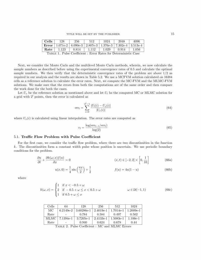
TITLE WILL BE SET BY THE PUBLISHER 15
Cells 128 256 512 1024 2048 4096Error 1.071e-2 6.090e-3 2.807e-3 1.376e-3 7.302e-4 3.513e-4Rate 1.123 0.814 1.112 1.029 0.914 1.056Table 1. Pulse Coefficient : Error Rates for Deterministic Case
Next, we consider the Monte Carlo and the multilevel Monte Carlo methods, wherein, we now calculate thesample numbers as described before using the experimental convergence rates of 0.5 and calculate the optimalsample numbers. We then verify that the deterministic convergence rates of the problem are above 1/2 asrequired in our analysis and the results are shown in Table 5.2. We use a MCFVM solution calculated on 16384cells as a reference solution to calculate the error rates. Next, we compute the MC-FVM and the MLMC-FVMsolutions. We make sure that the errors from both the computations are of the same order and then comparethe work done for the both the cases.
Let Ue be the reference solution as mentioned above and let Ul be the computed MC or MLMC solution fora grid with 2l points, then the error is calculated as
errl =
2l−1∑i=0
|Ul(i)− Ue(i)||Ue(i)|
(64)
where Ue(i) is calculated using linear interpolation. The error rates are computed as
rl =log(errl−1/errl)
log(2)(65)
5.1. Traffic Flow Problem with Pulse Coefficient
For the first case, we consider the traffic flow problem, where there are two discontinuities in the functionk. The discontinuities form a constant width pulse whose position is uncertain. We use periodic boundaryconditions for the problem.
∂u
∂t+∂k(ω;x)f(u)
∂x= 0 (x, t) ∈ [−2, 2]×
[0,
1
10
](66a)
u(x, 0) =1
4sin(πx
2
)+
1
2f(u) = 4u(1− u) (66b)
where
k(ω, x) =
1 if x < −0.5 + ω
2 if − 0.5 + ω ≤ x < 0.5 + ω
1 if 0.5 + ω ≤ xω ∈ U(−1, 1) (66c)
Cells 64 128 256 512 1024MC 6.2149e-2 3.60286e-1 2.4019e-1 1.7014e-1 1.2009e-1Rate - 0.784 0.584 0.497 0.502
MLMC 7.1394e-1 3.7205e-1 2.4133e-1 1.5083e-1 1.106e-1Rate - 0.940 0.624 0.678 0.44
Table 2. Pulse Coefficient : MC and MLMC Errors

16 TITLE WILL BE SET BY THE PUBLISHER
0
0.2
0.4
0.6
0.8
1
-2 -1.5 -1 -0.5 0 0.5 1 1.5 2
u
x
VarianceMean
Figure 1. Traffic Flow Problem with Pulse Function Coefficient
Cells 64 128 256 512 1024MC 4 18.52 135 1092 8490Rate - 2.211 2.865 3.015 2.958
MLMC 5.5 15.02 40 132 489Rate - 1.449 1.413 1.722 1.889
Table 3. Pulse Coefficient : MC and MLMC Work (in compute seconds)
5.2. Traffic Flow Problem with a Brownian Bridge with Jumps Coefficient
For the second example, we consider the case where the coefficient k is given by a Brownian Bridge withJumps. We construct such a bridge from a Brownian bridge pinned at both ends by adding discontinuitiesat random points in the interval. Let b(x) be a Brownian bridge pinned at 2 at x = −2, 2. Next, we startintroducing jumps of random magnitude hj in the Brownian bridge b(x) at random points xj , j = 1, 2, . . . , n.We ensure that the number of jumps are finite and that b(x) > 1 to fulfill the condition k(x) > 1. The resultantfunction B(x) can be written as
B(x) = b(x) +
j∑k=0
hk for xj < x < xj+1, x0 = −2, xn+1 = 2 (67)

TITLE WILL BE SET BY THE PUBLISHER 17
Cells 128 256 512 1024 2048 4096Error 2.665e-2 1.423e-2 8.438e-3 4.855e-3 2.678e-3 1.325e-3Rate 0.662 0.900 0.758 0.797 0.858 1.015
Table 4. Brownian Bridge with Jumps : Error Rates for Deterministic Case
∂u
∂t+∂k(ω;x)f(u)
∂x= 0 (x, t) ∈ [−2, 2]×
[0,
1
10
](68a)
u(x, 0) =1
4sin(πx
2
)+
1
2f(u) = 4u(1− u) (68b)
Cells 64 128 256 512 1024MC-FVM 2.132e-1 1.3872e-1 1.003e-1 7.6139e-2 5.7780e-2
Rate - 0.620 0.467 0.397 0.398MLMC-FVM 2.3452e-1 1.3925e-1 9.8519e-2 6.6764e-2 5.299e-1
Rate - 0.752 0.499 0.561 0.335Table 5. Brownian Bridge with Jumps : MC and MLMC Errors
Cells 64 128 256 512 1024MC-FVM 6.7 31.58 254 2012 16380
Rate - 2.236 3.001 2.986 3.025MLMC-FVM 10.82 30.85 64 252 922
Rate - 1.511 1.052 1.977 1.871
Table 6. Brownian Bridge with Jumps : MC and MLMC Work (in compute second)
6. Conclusion
In this paper, we have considered a scalar conservation law with discontinuous flux in space in one dimen-sion. We have defined a random entropy solution for the conservation law and have proved its existence anduniqueness. Further, we have adapted the Multilevel Monte Carlo Finite Volume Method for the problem andhave compared its performance with the Monte Carlo Finite Volume Method, wherein, we have shown that theMultilevel Monte Carlo Method behaves as expected in the theoretical analysis. In particular, we show thatthe Multilevel Monte Carlo method is a more efficient alternative to Monte Carlo methods.
The work of Jayesh Badwaik is supported by German Priority Programme 1648 (SPPEXA). The work of Nils HenrikRisebro was performed while visiting University of Wurzburg during Spring of 2017. During this time, he was supportedby Giovanni-Prodi Chair Position at Wurzburg University. The work of Christian Klingenberg was supported by GermanAcademic Exchange Service and Research Council of Norway.
References
[1] Remi Abgrall. A simple, flexible and generic deterministic approach to uncertainty quantifications in non linear problems:application to fluid flow problems. 2008.
[2] Adimurthi, Rajib Dutta, Shyam Sundar Ghoshal, and G. D. Veerappa Gowda. Existence and nonexistence of TV bounds for
scalar conservation laws with discontinuous flux. Communications on Pure and Applied Mathematics, 64(1):84–115, 2011.

18 TITLE WILL BE SET BY THE PUBLISHER
1
1.5
2
2.5
3
-2 -1.5 -1 -0.5 0 0.5 1 1.5 2
u
k(x)
k(x)
Figure 2. One Instance of Brownian Bridge with Jumps
[3] Boris Andreianov, Kenneth Hvistendahl Karlsen, and Nils Henrik Risebro. A theory of l1-dissipative solvers for scalar conser-
vation laws with discontinuous flux. Archive for rational mechanics and analysis, 201(1):27–86, 2011.
[4] Alberto Bressan. Hyperbolic systems of conservation laws, volume 20 of Oxford Lecture Series in Mathematics and its Appli-cations. Oxford University Press, Oxford, 2000. The one-dimensional Cauchy problem.
[5] R. Burger, K. H. Karlsen, C. Klingenberg, and N. H. Risebro. A front tracking approach to a model of continuous sedimentation
in ideal clarifier-thickener units. Nonlinear Analysis. Real World Applications. An International Multidisciplinary Journal,4(3):457–481, 2003.
[6] Raimund Burger and Wolfgang L Wendland. Sedimentation and suspension flows: Historical perspective and some recent
developments. Journal of Engineering Mathematics, 41(2):101–116, 2001.[7] Qian-Yong Chen, David Gottlieb, and Jan S Hesthaven. Uncertainty analysis for the steady-state flows in a dual throat nozzle.
Journal of Computational Physics, 204(1):378–398, 2005.
[8] Constantine M Dafermos. Hyperbolic conservation laws in continuum physics, volume 325 of grundlehren der mathematischenwissenschaften [fundamental principles of mathematical sciences], 2010.
[9] Stefan Diehl. A conservation law with point source and discontinuous flux function modelling continuous sedimentation. SIAM
Journal on Applied Mathematics, 56(2):388–419, 1996.[10] Tore Gimse and Nils Henrik Risebro. Solution of the cauchy problem for a conservation law with a discontinuous flux function.
SIAM Journal on Mathematical Analysis, 23(3):635–648, 1992.[11] William G Gray. General conservation equations for multi-phase systems: 4. constitutive theory including phase change.
Advances in Water Resources, 6(3):130–140, 1983.
[12] BD Greenshields, Ws Channing, Hh Miller, et al. A study of traffic capacity. In Highway research board proceedings, volume1935. National Research Council (USA), Highway Research Board, 1935.
[13] M Hassanizadeh and WG Gray. General conservation equations for multi-phase system: 2. mass, momenta, energy and entropyequations. Advances in Water Resources, 2:191–203, 1979.
[14] Majid Hassanizadeh and William G Gray. General conservation equations for multi-phase systems: 1. averaging procedure.Advances in water resources, 2:131–144, 1979.
[15] Majid Hassanizadeh and William G Gray. General conservation equations for multi-phase systems: 3. constitutive theory forporous media flow. Advances in Water Resources, 3(1):25–40, 1980.
[16] Helge Holden and Nils Henrik Risebro. Front tracking for hyperbolic conservation laws, volume 152. Springer, 2015.

TITLE WILL BE SET BY THE PUBLISHER 19
0
0.2
0.4
0.6
0.8
1
-2 -1.5 -1 -0.5 0 0.5 1 1.5 2
u
x
VarianceMean
Figure 3. Traffic Flow Problem with Brownian Bridge with Jumps
[17] Kenneth H Karlsen and John D Towers. Convergence of the lax-friedrichs scheme and stability for conservation laws with adiscontinuous space-time dependent flux. Chinese Annals of Mathematics, 25(03):287–318, 2004.
[18] Runhild Aae Klausen and Nils Henrik Risebro. Stability of conservation laws with discontinuous coefficients. Journal of
differential equations, 157(1):41–60, 1999.[19] U. Koley, N. H. Risebro, Ch. Schwab, and F. Weber. Multilevel monte carlo for random degenerate scalar convection diffusion
equation.
[20] Michel Ledoux and Michel Talagrand. Probability in Banach Spaces: isoperimetry and processes. Springer Science & BusinessMedia, 2013.
[21] Randall J LeVeque, David L George, and Marsha J Berger. Tsunami modelling with adaptively refined finite volume methods.
Acta Numerica, 20:211–289, 2011.[22] Michael J Lighthill and Gerald Beresford Whitham. On kinematic waves. ii. a theory of traffic flow on long crowded roads. In
Proceedings of the Royal Society of London A: Mathematical, Physical and Engineering Sciences, volume 229, pages 317–345.
The Royal Society, 1955.[23] G Lin, CH Su, and GE Karniadakis. The stochastic piston problem. Proceedings of the National Academy of Sciences of the
United States of America, 101(45):15840–15845, 2004.[24] Xiang Ma and Nicholas Zabaras. An adaptive hierarchical sparse grid collocation algorithm for the solution of stochastic
differential equations. Journal of Computational Physics, 228(8):3084–3113, 2009.[25] Siddhartha Mishra, Nils Henrik Risebro, Christoph Schwab, and Svetlana Tokareva. Numerical solution of scalar conservation
laws with random flux functions. SIAM/ASA Journal on Uncertainty Quantification, 4(1):552–591, 2016.[26] Siddhartha Mishra and Ch Schwab. Sparse tensor multi-level monte carlo finite volume methods for hyperbolic conservation
laws with random initial data. Mathematics of Computation, 81(280):1979–2018, 2012.[27] Gael Poette, Bruno Despres, and Didier Lucor. Uncertainty quantification for systems of conservation laws. Journal of Com-
putational Physics, 228(7):2443–2467, 2009.
[28] Paul I Richards. Shock waves on the highway. Operations research, 4(1):42–51, 1956.[29] John D Towers. Convergence of a difference scheme for conservation laws with a discontinuous flux. SIAM journal on numerical
analysis, 38(2):681–698, 2000.

20 TITLE WILL BE SET BY THE PUBLISHER
[30] JMAM Van Neerven. Stochastic evolution equations. ISEM lecture notes, 2008.[31] Xiaoliang Wan and George Em Karniadakis. Long-term behavior of polynomial chaos in stochastic flow simulations. Computer
methods in applied mechanics and engineering, 195(41):5582–5596, 2006.
[32] Jeroen AS Witteveen, Alex Loeven, and Hester Bijl. An adaptive stochastic finite elements approach based on newton–cotesquadrature in simplex elements. Computers & Fluids, 38(6):1270–1288, 2009.


![Spatial-Spectral Operator Theoretic Methods for ...jjb/spatial_spectral_gem.pdf · spatially motivated [37], multilevel segmentation [9] or combining segmentation with pixel classi](https://static.fdocuments.us/doc/165x107/5f3258347ce0fe3ee12e38bd/spatial-spectral-operator-theoretic-methods-for-jjbspatialspectralgempdf.jpg)