Automatic vehicle classi cation using appearance based ... · Automatic vehicle classi cation using...
87
Imagem Ant´ onio Carlos Gomes Rodrigues Marques Sim˜ oes Automatic vehicle classification using appearance based features Master’s Degree in Electrical and Computer Engineering September 2015
Transcript of Automatic vehicle classi cation using appearance based ... · Automatic vehicle classi cation using...

Imagem
Antonio Carlos Gomes Rodrigues Marques Simoes
Automatic vehicle classification using
appearance based features
Master’s Degree in Electrical and Computer Engineering
September 2015

Departamento de Engenharia Electrotecnica e de ComputadoresFaculdade de Ciencias e Tecnologia
Universidade de Coimbra
A DissertationMaster’s Degree in Electrical and Computer Engineering/
Automatic vehicle classification using
appearance based features
Antonio Carlos Gomes Rodrigues Marques Simoes
Research Developed Under Supervision ofProf. Doutor Jorge Manuel Moreira de Campos Pereira Batista
JuryProf. Doutor Helder de Jesus Araujo and
Prof. Doutor Nuno Miguel Mendonca da Silva Goncalves
September 2015


Work developed in the Institute of Systems and Robotics of the University of Coimbra.


Thanks
I’d like to start by thanking all the people who’ve in one way or another have helped me through-
out this work. A special thank to my supervisor Prof. Jorge Baptista for guiding me through
this journey and for all his support. To my colleagues in the Computer Vision Lab and in Insti-
tute of Systems and Robotics: Pedro Martins, Joao Faro, Joao Henrique, Patrick Brandao, Luıs
Garrote e Mario Vieira. Your friendliness and willingness to assist me when necessary made it
much easier to overcome certain hurdles. I’d also like to thank my family for, without them, I
wouldn’t have had the chance to write these words. On a final note, I would like to thank Brisa
for providing the majority of the images used in this work, as well as for their willingness to
answer our questions.


Abstract
Vehicle classification has been a highly focused topic amongst the scientific community due to its
application in automatic tolling systems, road surveillance, traffic monitoring, etc. Image-based
classification using computer vision techniques provides a non-invasive, cost effective, automated
option to these systems. In traffic video surveillance systems vehicle detection and classification
help provide more accurate and detailed statistics that can be used in intelligent transport sys-
tems.
We implemented a non-invasive vision based vehicle classification system able to operate in both
multilane free flow environments and in toll stations. Additionally, it can be used in surveillance
cameras present in various motorways to provide not only quantitative information about flowing
traffic but also qualitative.
In this work we implement three hog-based descriptors as well as an additional edge points groups
SIFT-based descriptor. These were tested on four distinct datasets captured using cameras al-
ready present in tolling/surveillance locations in various motorways.
We were able to obtain an average of 97% accuracy using a global HOG descriptor. Using mul-
tiple SVM trained with local HOG descriptors we slightly improved results when high quality
images were used, but more importantly showed the potential application of this method when
well localized highly descriminatory sections of an object exist. Additionally we showed that the
HOG-based descriptors classification was able to outperform the SIFT-based edge points groups
across all datasets.
Keywords: Computer Vision, Machine Learning, Vehicle Classification.


Resumo
A classificacao de veıculos tem sido um topico muito focado pela comunidade cientıfica devido
a sua aplicacao em sistemas de portagens automaticas, vigilancia, monotorizacao de trafico, etc.
Classificacao baseada em imagem usando tecnicas de visao por computer fornece uma opccao nao
invasica, de baixo custo e automatica a estes sistemas. Em sistemas de monotorizacao de trafego,
deteccao e classificacao de veıculos ajudam a fornecer estatisticas mais detalhadas e exatas que
podem ser usadas em sistemas de transporte inteligentes.
Implementamos um sistema de classificacao baseado em image nao invasivo e que e capaz de
operar em ambientes de circulacao livre bem como em portagens. Alem disso, o sistema pode
ser usado em cameras de vigilancia presents em varias estradas de forma a fornecer nao apenas
informacao quantitativa acerca do trafego, mas tambem informacao quantitativa.
Neste trabalho implementamos tres descritores baseado em HOG (histograma de gradientes ori-
entados) bem como um descritor adicional de grupos de points fronteira baseado em SIFT (trans-
formada de caracterısticas invariantes a escala). Estes descritores foram testados usando quatro
conjuntos de dados constituıdos por images capturadas usando cameras ja instaladas (para out-
ras tarefas) em portagens e outras localizacoes.
Obtemos em media uma 97% de classificacoes correctas usando um descriptor HOG global, 95%
usando um descritor HOG em piramide. Conseguimos melhorar ligeiramente os resultados usando
um sistema com multiplos classificadores SVM (maquinas de vectores de suporte) treinados com
descritores HOG locais. Mais importante mostramos o potencial deste metodo quando existem
seccoes bem localizadas e altamente descriminadoras de um objecto. Por fim mostramos que a
classificacao que usou descritores baseados em HOG obteve melhores resultados que o metodo de
classificacao baseado em grupos de pontos de fronteira em todos os conjuntos de dados testados.
Palavras Chave: Visao por Computador, Apredizagem de Maquina, Classificacao de Veıculos.


Contents
1 Introduction 1
1.1 Motivation . . . . . . . . . . . . . . . . . . . . . . . . . . . . . . . . . . . . . . . . 1
1.2 Main contributions . . . . . . . . . . . . . . . . . . . . . . . . . . . . . . . . . . . 2
1.3 Structure of the thesis . . . . . . . . . . . . . . . . . . . . . . . . . . . . . . . . . 2
2 State of the Art 3
2.1 Vehicle Classification . . . . . . . . . . . . . . . . . . . . . . . . . . . . . . . . . . 3
2.2 Brisa’s Current System . . . . . . . . . . . . . . . . . . . . . . . . . . . . . . . . . 5
3 Datasets’ Description 7
3.1 Rear View . . . . . . . . . . . . . . . . . . . . . . . . . . . . . . . . . . . . . . . . 7
3.1.1 Toll Stations . . . . . . . . . . . . . . . . . . . . . . . . . . . . . . . . . . . 7
3.1.2 Multi-Lane Free Flow . . . . . . . . . . . . . . . . . . . . . . . . . . . . . . 9
3.2 Frontal View . . . . . . . . . . . . . . . . . . . . . . . . . . . . . . . . . . . . . . 9
3.3 Top Side View . . . . . . . . . . . . . . . . . . . . . . . . . . . . . . . . . . . . . . 10
4 Descriptors 13
4.1 Histogram of Oriented Gradients . . . . . . . . . . . . . . . . . . . . . . . . . . . 14
4.1.1 Global HOG descriptors . . . . . . . . . . . . . . . . . . . . . . . . . . . . 15
4.1.2 Pyramid HOG descriptors . . . . . . . . . . . . . . . . . . . . . . . . . . . 15
4.1.3 Local HOG descriptors . . . . . . . . . . . . . . . . . . . . . . . . . . . . . 16
i

4.2 Edge Points Groups of SIFT descriptors . . . . . . . . . . . . . . . . . . . . . . . 17
5 Classifiers 19
5.1 Support Vector Machine . . . . . . . . . . . . . . . . . . . . . . . . . . . . . . . . 20
5.1.1 Linear SVM . . . . . . . . . . . . . . . . . . . . . . . . . . . . . . . . . . . 20
5.1.2 Multiclass Classification . . . . . . . . . . . . . . . . . . . . . . . . . . . . 22
5.1.2.1 One versus All . . . . . . . . . . . . . . . . . . . . . . . . . . . . 23
5.1.2.2 One versus One . . . . . . . . . . . . . . . . . . . . . . . . . . . . 23
5.2 Constellation Model . . . . . . . . . . . . . . . . . . . . . . . . . . . . . . . . . . 23
5.2.1 Implicit Shape Model . . . . . . . . . . . . . . . . . . . . . . . . . . . . . . 24
5.2.2 Learning and recognition . . . . . . . . . . . . . . . . . . . . . . . . . . . . 25
6 Development 27
6.1 Rear View with Toll Stations . . . . . . . . . . . . . . . . . . . . . . . . . . . . . 27
6.1.1 Original Images . . . . . . . . . . . . . . . . . . . . . . . . . . . . . . . . . 27
6.1.1.1 Global HOG descriptors . . . . . . . . . . . . . . . . . . . . . . . 27
6.1.1.2 Local HOG descriptors . . . . . . . . . . . . . . . . . . . . . . . . 30
6.1.1.3 PHOG descriptors . . . . . . . . . . . . . . . . . . . . . . . . . . 32
6.1.2 Segmented Images . . . . . . . . . . . . . . . . . . . . . . . . . . . . . . . 33
6.1.2.1 Global HOG descriptor . . . . . . . . . . . . . . . . . . . . . . . 33
6.1.2.2 Local HOG descriptor . . . . . . . . . . . . . . . . . . . . . . . . 34
6.1.2.3 PHOG descriptor . . . . . . . . . . . . . . . . . . . . . . . . . . . 35
6.1.2.4 Edge group SIFT based descriptor . . . . . . . . . . . . . . . . . 36
6.1.3 Comparative Evaluation and discussion . . . . . . . . . . . . . . . . . . . . 37
6.2 Rear View Multi-Lane Free Flow . . . . . . . . . . . . . . . . . . . . . . . . . . . 37
6.2.1 Original Images . . . . . . . . . . . . . . . . . . . . . . . . . . . . . . . . . 38
6.2.1.1 Global HOG descriptors . . . . . . . . . . . . . . . . . . . . . . . 38
ii
6.2.1.2 Local HOG descriptors . . . . . . . . . . . . . . . . . . . . . . . . 39
6.2.1.3 PHOG descriptors . . . . . . . . . . . . . . . . . . . . . . . . . . 40
6.2.2 Segmented Images . . . . . . . . . . . . . . . . . . . . . . . . . . . . . . . 40
6.2.2.1 Global HOG descriptors . . . . . . . . . . . . . . . . . . . . . . . 41
6.2.2.2 Local HOG descriptors . . . . . . . . . . . . . . . . . . . . . . . . 41
6.2.2.3 PHOG descriptor . . . . . . . . . . . . . . . . . . . . . . . . . . . 43
6.2.2.4 Edge group SIFT based descriptor . . . . . . . . . . . . . . . . . 44
6.2.3 Comparative Evaluation and discussion . . . . . . . . . . . . . . . . . . . . 44
6.3 Frontal View . . . . . . . . . . . . . . . . . . . . . . . . . . . . . . . . . . . . . . 45
6.3.1 Original Images . . . . . . . . . . . . . . . . . . . . . . . . . . . . . . . . . 45
6.3.1.1 Global HOG descriptor . . . . . . . . . . . . . . . . . . . . . . . 45
6.3.1.2 Local HOG descriptors . . . . . . . . . . . . . . . . . . . . . . . . 46
6.3.1.3 PHOG descriptors . . . . . . . . . . . . . . . . . . . . . . . . . . 48
6.3.2 Segmented Images . . . . . . . . . . . . . . . . . . . . . . . . . . . . . . . 48
6.3.2.1 License Plate Localization . . . . . . . . . . . . . . . . . . . . . . 48
6.3.2.2 Global HOG descriptor . . . . . . . . . . . . . . . . . . . . . . . 50
6.3.2.3 Local HOG descriptors . . . . . . . . . . . . . . . . . . . . . . . . 51
6.3.2.4 PHOG . . . . . . . . . . . . . . . . . . . . . . . . . . . . . . . . . 52
6.3.2.5 Edge group SIFT based descriptor . . . . . . . . . . . . . . . . . 53
6.3.3 Comparative Evaluation and discussion . . . . . . . . . . . . . . . . . . . . 54
6.4 Top Side View . . . . . . . . . . . . . . . . . . . . . . . . . . . . . . . . . . . . . . 55
6.4.1 Global HOG descriptors . . . . . . . . . . . . . . . . . . . . . . . . . . . . 55
6.4.2 Local HOG descriptor . . . . . . . . . . . . . . . . . . . . . . . . . . . . . 57
6.4.3 PHOG descriptor . . . . . . . . . . . . . . . . . . . . . . . . . . . . . . . . 57
6.4.4 Edge group SIFT based descriptor . . . . . . . . . . . . . . . . . . . . . . 57
iii

7 Conclusions 59
Acronyms and symbols 65
iv

List of Figures
2.1 Brisa’s classification criteria. Motorcycles are considered class 5 in electronic tolling. 5
3.1 Rear View with Toll Stations dataset image samples. . . . . . . . . . . . . . . . . 8
3.2 Rear View with Toll Stations Dataset class distribution. . . . . . . . . . . . . . . . 8
3.3 Multi-Lane Free Flow dataset image samples. . . . . . . . . . . . . . . . . . . . . 9
3.4 Rear View Multi-lane Free Flow Dataset Distribution. . . . . . . . . . . . . . . . . 10
3.5 Frontal View dataset image samples. . . . . . . . . . . . . . . . . . . . . . . . . . 10
3.6 Frontal View Dataset Distribution. . . . . . . . . . . . . . . . . . . . . . . . . . . 11
3.7 Top Side View dataset image samples. . . . . . . . . . . . . . . . . . . . . . . . . 11
3.8 Background subtraction mask. . . . . . . . . . . . . . . . . . . . . . . . . . . . . . 12
3.9 Virtual sensor display. . . . . . . . . . . . . . . . . . . . . . . . . . . . . . . . . . 12
3.10 Frontal View Dataset Distribution. . . . . . . . . . . . . . . . . . . . . . . . . . . 12
4.1 Visualization of HOG features. . . . . . . . . . . . . . . . . . . . . . . . . . . . . . 15
4.2 Visualization of PHOG. Image taken from https://www.robots.ox.ac.uk/\protect\
unhbox\voidb@x\penalty\@M\vgg/research/caltech/phog.html . . . . . . . 16
4.3 Regular and irregular divisions of the image. . . . . . . . . . . . . . . . . . . . . . 17
4.4 Visualization of SIFT descriptors.. Image from http://www.codeproject.com/
KB/recipes/619039/SIFT.JPG . . . . . . . . . . . . . . . . . . . . . . . . . . . . 18
5.1 Visualization of separating line for 2D data. Image taken from wikipedia. . . . . . 20
6.1 Results obtained using different percentages of total number of samples as training. 28
v

6.2 Image showing the different sections of the image used to train the different classifiers. 30
6.3 Rear View with Toll Stations images samples after segmentation . . . . . . . . . . 33
6.4 Rear View with Toll Stations Dataset class distribution using correct license plate
location. . . . . . . . . . . . . . . . . . . . . . . . . . . . . . . . . . . . . . . . . . 34
6.5 Graph comparing the performances of the system using the different descriptors
on the original unsegmented images. . . . . . . . . . . . . . . . . . . . . . . . . . 37
6.6 Graph comparing the performances of the system using the different descriptors
on the segmented images. . . . . . . . . . . . . . . . . . . . . . . . . . . . . . . . 38
6.7 Samples of segmented images from Rear View Multi-lane Free Flow Dataset. . . . 40
6.8 Sections in segmented image of the Rear View Multi-lane Free Flow Dataset. . . . 41
6.9 Results obtained using different percentages of total number of samples as training 44
6.10 Results obtained using different percentages of total number of samples as training 45
6.11 Image showing the different sections of the image used to train the different classifiers. 47
6.12 All pixels within the threshold of the reference value. . . . . . . . . . . . . . . . . 49
6.13 Pixels remaining after applying filter. . . . . . . . . . . . . . . . . . . . . . . . . . 49
6.14 Frontal View dataset images samples after segmentation. . . . . . . . . . . . . . . 50
6.15 Image showing the irregular sections of the image used to train the different clas-
sifiers. . . . . . . . . . . . . . . . . . . . . . . . . . . . . . . . . . . . . . . . . . . 51
6.16 Graph comparing the performances of the system using the different descriptors
on the original unsegmented images. . . . . . . . . . . . . . . . . . . . . . . . . . 54
6.17 Graph comparing the performances of the system using the different descriptors
on segmented images. . . . . . . . . . . . . . . . . . . . . . . . . . . . . . . . . . . 54
6.18 Top Side View Dataset distribution of ’Heavy’ and ’Light’ vehicles. . . . . . . . . 56
vi

List of Tables
2.1 Mapping between Brisa’s classes and classes used in our work. . . . . . . . . . . . 5
6.1 Confusion Matrix of Rear View with Toll Stations Dataset using 80% of samples
as training . . . . . . . . . . . . . . . . . . . . . . . . . . . . . . . . . . . . . . . . 28
6.2 Confusion Matrix with equal distribution of classes in the training samples. . . . . 29
6.3 Confusion Matrix with slightly bias distribution of classes in the training samples. 29
6.4 Confusion Matrix with slightly bias distribution of classes in the training samples
and a 0.4 ratio. . . . . . . . . . . . . . . . . . . . . . . . . . . . . . . . . . . . . . 30
6.5 Individual Classifiers Accuracy. . . . . . . . . . . . . . . . . . . . . . . . . . . . . 31
6.6 Confusion Matrix using the multiple classifiers for different sections in the image
for the Rear View with Toll Stations Dataset. . . . . . . . . . . . . . . . . . . . . 31
6.7 Confusion Matrix obtained using PHOG descriptors on original images of the Rear
View with Toll Stations Dataset. . . . . . . . . . . . . . . . . . . . . . . . . . . . 32
6.8 Confusion Matrix using global HOG descriptors segmented images of the Rear
View with Toll Stations Dataset. . . . . . . . . . . . . . . . . . . . . . . . . . . . 34
6.9 Individual Classifiers Accuracy . . . . . . . . . . . . . . . . . . . . . . . . . . . . . 35
6.10 Confusion Matrix using the multiple classifiers for different sections in the image
for the segmented Rear View with Toll Stations Dataset. . . . . . . . . . . . . . . 35
6.11 Confusion Matrix using PHOG descriptors on segmented images of the Rear View
with Toll Stations Dataset. . . . . . . . . . . . . . . . . . . . . . . . . . . . . . . . 36
6.12 Confusion Matrix using the edge points groups descriptor in segmented images of
the Rear View with Toll Stations Dataset. . . . . . . . . . . . . . . . . . . . . . . 36
vii

6.13 Confusion Matrix when using a training samples ratio of 0.8. . . . . . . . . . . . . 38
6.14 Confusion Matrix when using normalized distribution in the training samples. . . 38
6.15 Confusion Matrix ’Cars’ vs ’Vans’. . . . . . . . . . . . . . . . . . . . . . . . . . . 39
6.16 Confusion Matrix when using only day images . . . . . . . . . . . . . . . . . . . . 39
6.17 Confusion Matrix using PHOG descriptor on segmented images of the Front View
Dataset. . . . . . . . . . . . . . . . . . . . . . . . . . . . . . . . . . . . . . . . . . 40
6.18 Confusion Matrix using global HOG descriptor on segmented images of Rear View
Multilane Free Flow Dataset. . . . . . . . . . . . . . . . . . . . . . . . . . . . . . 41
6.19 Individual Classifiers Accuracy. . . . . . . . . . . . . . . . . . . . . . . . . . . . . 42
6.20 Confusion Matrix using the multiple classifiers for different sections in the image
for the segmented Rear View Multi-lane Free Flow Dataset. . . . . . . . . . . . . 42
6.21 Behaviour of final results when the classifier’s confidence was below 0.65. . . . . . 42
6.22 Confusion Matrix using PHOG descriptors on segmented images from Rear View
Multi-lane Free Flow Dataset. . . . . . . . . . . . . . . . . . . . . . . . . . . . . . 43
6.23 Confusion Matrix using Edge based SIFT . . . . . . . . . . . . . . . . . . . . . . . 44
6.24 Confusion Matrix of Front View Dataset using 80% of samples as training. . . . . 46
6.25 Confusion Matrix of Front View Dataset using normalization of training samples
distribution using 50% of the dataset as training samples. . . . . . . . . . . . . . . 46
6.26 Individual Classifiers Accuracy . . . . . . . . . . . . . . . . . . . . . . . . . . . . . 47
6.27 Confusion Matrix using local HOG descriptors on segmented images of the Front
View Dataset. . . . . . . . . . . . . . . . . . . . . . . . . . . . . . . . . . . . . . . 47
6.28 Confusion Matrix using PHOG descriptors on segmented images of the Front View
Dataset. . . . . . . . . . . . . . . . . . . . . . . . . . . . . . . . . . . . . . . . . . 48
6.29 Confusion Matrix using global HOG descriptors segmented images of the Front
View Dataset . . . . . . . . . . . . . . . . . . . . . . . . . . . . . . . . . . . . . . 50
6.30 Confusion Matrix using local HOG descriptors on segmented images of the Front
View Dataset with regular division. . . . . . . . . . . . . . . . . . . . . . . . . . . 51
6.31 Individual Classifiers Accuracy. . . . . . . . . . . . . . . . . . . . . . . . . . . . . 52
viii

6.32 Confusion Matrix using local HOG descriptors on segmented images of the Front
View Dataset with irregular division. . . . . . . . . . . . . . . . . . . . . . . . . . 52
6.33 Behaviour of final results when the classifier’s confidence was below 0.65. . . . . . 52
6.34 Confusion Matrix using PHOG descriptor on segmented images of the Front View
Dataset. . . . . . . . . . . . . . . . . . . . . . . . . . . . . . . . . . . . . . . . . . 53
6.35 Confusion Matrix using Edge group SIFT based descriptor on segmented images
of the Front View Dataset. . . . . . . . . . . . . . . . . . . . . . . . . . . . . . . . 53
6.36 Confusion Matrix using 80% samples for training. . . . . . . . . . . . . . . . . . . 55
6.37 Confusion Matrix using normalized distribution of training samples. . . . . . . . . 56
6.38 Confusion Matrix using two broader classes. . . . . . . . . . . . . . . . . . . . . . 56
6.39 Confusion Matrix using PHOG descriptor on Top Side View Dataset images. . . . 57
6.40 Confusion Matrix using PHOG descriptors and two broader classes. . . . . . . . . 57
6.41 Confusion Matrix using edge points groups descriptor . . . . . . . . . . . . . . . . 58
6.42 Confusion Matrix using two classes ’heavy’ vs ’light’ filtering edges using an image
mask. . . . . . . . . . . . . . . . . . . . . . . . . . . . . . . . . . . . . . . . . . . 58
6.43 Confusion Matrix using two classes ’heavy’ vs ’light’ without filtering edges using
an image mask. . . . . . . . . . . . . . . . . . . . . . . . . . . . . . . . . . . . . . 58
ix

x

Chapter 1
Introduction
1.1 Motivation
Vehicle traffic surveillance has attracted significant interest in the computer vision community
due to its high number of possible applications. Important statistics such as traffic density,
queueing, average speed of vehicles could all be extracted from surveillance cameras and used
in an intelligent transport system (ITS). Another important situation where computer vision
can make a difference is when dangerous situations occur, they can be detected much quicker
enabling a prompt response. In 2009, there were 10.8 million recorded traffic accidents in the
United States alone resulting in 33808 deaths [5]. An early notification could significantly improve
survival rate in these situations [10]. Automatic tolling systems can also benefit from computer
vision techniques. In 2014, according to the European Association of Tolled Motorways, Bridges
and Tunnels [34], there were more than 45500km of tolled ways in Europe with about 16300
toll lanes. Some methods of vehicle classification currently being used [21] are invasive, which
means they require some hardware to be installed on the pavement. Despite achieving great
results, this situation proves problematic when maintenance is required as it involves stopping
traffic. Non-invasive methods are also used to some extent [35], however they often require
precision hardware which can be expensive. With the development of image/video technology,
image-based classification provides a robust, non-invasive alternative to these methods. The
great majority of tolling locations already have cameras installed for surveillance and security
reasons, which means that applying this type of vehicle classification would come with little to
no added cost.
1
In our work we will focus on using images from these pre-installed cameras to classify vehicles
into five general classes such as ’cars’, ’vans’, ’trucks’, ’motos’ and ’buses’. Even though most
motorways operators have their own classification criteria we feel that these five categories are
suited as they often tend to match classes defined by the motorway operators giving it a wider
application range.
1.2 Main contributions
We developed a non-invasive image-based vehicle classification system and investigated its via-
bility when using pre-installed surveillance cameras in tolling locations. Three different datasets
were manually labelled throughout the project and an additional dataset was created by extract-
ing vehicles from a CCTV (Closed-Circuit TeleVision) surveillance video feed. For the duration
of our work we noted that it was difficult to find publicly available datasets suited for vehicle
classification. For this reason we will make the dataset we created publicly available to be used
in similar projects.
We implemented three HOG-based descriptors (global HOG, Local HOG, PHOG) which were
used in combination with SVM classifiers. Additionally we extended the work of Ma and Grimson
[24] to up to five classes in order to use it in our work. We were able to achieve as high as 97%
accuracy using HOG-based descriptors and 95% using Ma and Grimson’s constellation model.
1.3 Structure of the thesis
The organization of this thesis was devised with the objective of introducing the various com-
ponents of a object classification system sequentially and in a easy to consult manner. Chapter
2 goes over relevant research developed in the area as well the current system implemented by
Brisa [19] in many Portuguese highways. In chapter 3 the datasets used in this work are de-
scribed. Chapter 4 goes over the theoretical background of the descriptors used throughout our
work as well as how they were implemented. Similarly, in chapter 5 we can find the different
classifier methods used. Chapter 6 presents the developed work and the results obtained. Finally,
in chapter 7 we draw some conclusions from the developed work and present key directions for
future work.
2

Chapter 2
State of the Art
Vehicle classification has received much attention by the scientific community in past years. Due
to the relative low cost of cameras, high performing image-based classification systems are highly
desired. As such a wide variety of approaches have been proposed in recent years.
2.1 Vehicle Classification
Image based classification techniques have been slowly but surely replacing other methods of
vehicle classification systems [21], [35] which are normally tailored at a single motorway operator’s
classification criteria. Xiang et al [35] use a pair of infra-red laser emitter and receiver to count
a vehicles axles. Their system uses this information to label a vehicle into one of the 12 distinct
classes defined by Austroads [2]. Most recent approaches to vehicle classification attempt to
either classify vehicles into boarder categories like van, truck, car [15], [1], [24], [8] or try to
determine the vehicle make and model (ex: Fiat Punto) [9], [31], [29], [11], [36]
3D-model based approaches compute the vehicle’s 3D parameters to create a 3D-model of the
vehicle’s shape. In [3] the authors use gaussian mixture model to estimate background from
a CCTV video feed. The contours of the foreground blobs are then compared with existing
vehicle models and maximum overlap gives the final estimation. Two different types of models
were tested, project silhouettes and using HOG (histogram of Oriented Gradients) descriptors on
patches defined in a 3D-model space. This 3DHOG approach was able to deal with challenging
scenes where using motions silhouettes wielded the incorrect result.
Various PCA-based (Principal Component Analysis) approaches have also been proposed [37],
3

[1], [26]. Ambarkedar et al proposes three different approaches [1]. In PCA+DFVS (distance
from vehicle space) an eigenspace (vehicle space) is created for each class and the decision is
given by the closest distance out of all seperate vehicle spaces. In PCA+DIVS (distance in
vehicle space) a single vehicle space is created with all training samples regardless of label. By
projecting training images to this vehicle space a mean vector of weights (principal component)
is determined for each class. By calculating the Mahalanobis distance to each class’ mean vector
the final decision is made. Finally, in PCA+SVM (Support Vector Machine), after projecting
training images to a vehicle space as done in PCA+DIVS, instead of calculating a mean vector,
a SVM is trained using the training samples’ mean vectors. Peng et al in [26] used a similar
approach to PCA+DIVS in order to distinguish between five classes of vehicles based on their
frontal view. However, Peng et al also used K-means clustering to each class in order to decrease
intra-class variability by creating a number of sub-classes.
Appearance-based methods rely on extracting a set of features (HOG, SIFT, Sobel Edges) to
represent the vehicle’s appearance. Petrovic and Cotes [29] tested various edge-based features
including sobel response and square mapped gradients. These features together with simple
measure based decision modules like the dot product and euclidean distance were able to produce
interesting results detecting a vehicle’s make and model. Ma et al grouped modified SIFT
descriptors using mean shift technique to form repeatable edge group points. These points were
in turn used to create constellation models for each class and a Bayesian decision rule provided the
final classification. They were able to achieve high performance using low resolution surveillance
camera images. Zezhi et al [7] extracted individual vehicles from a CCTV video and used multiple
measures (ex: area, equivdiameter, disperseness) in combination with Pyramid Histogram of
Oriented Gradients (PHOG) to classify vehicles into multiple classes.
Methods relying on Neural Networks have also been recently emerging in the scientific community
[16], [13]. Dong et al in [16] propose a biologically inspired multi-layer feed forward convolutional
neural network. Their method is able to automatically learn good features which are discriminant
enough to work well in complex scenes. The softmax classifier is trained by multi-task learning
with small amounts of labelled data.
4
2.2 Brisa’s Current System
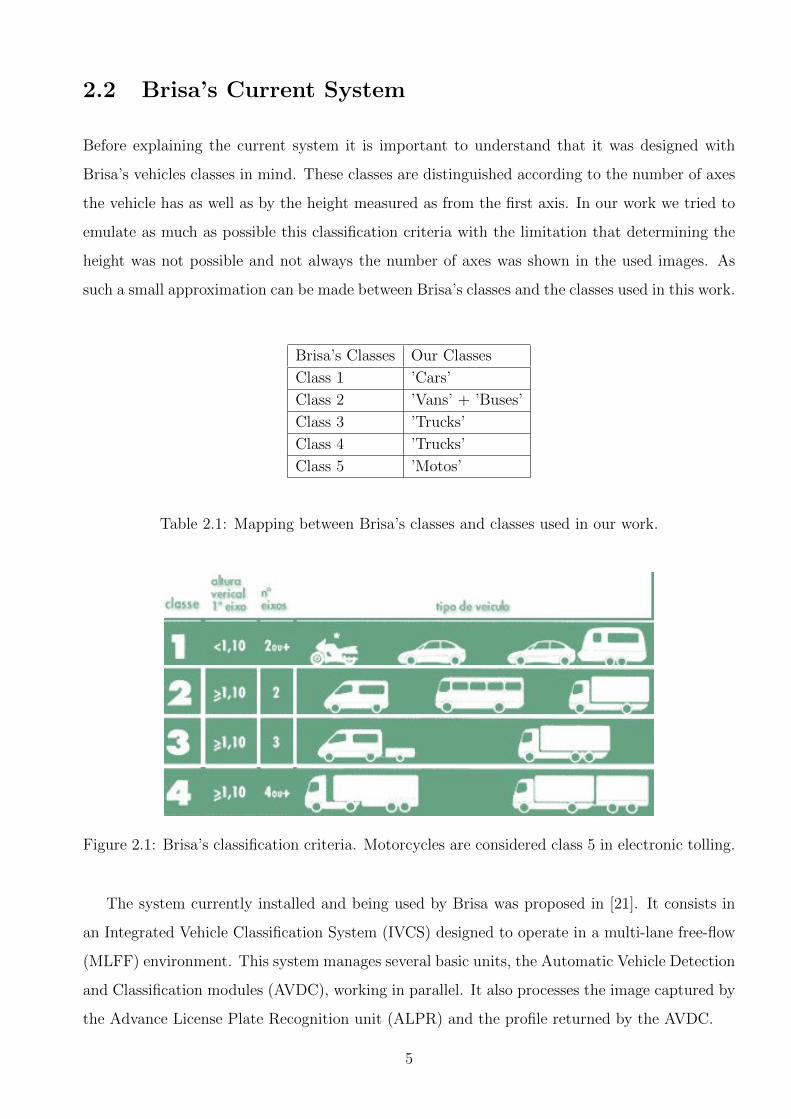
Before explaining the current system it is important to understand that it was designed with
Brisa’s vehicles classes in mind. These classes are distinguished according to the number of axes
the vehicle has as well as by the height measured as from the first axis. In our work we tried to
emulate as much as possible this classification criteria with the limitation that determining the
height was not possible and not always the number of axes was shown in the used images. As
such a small approximation can be made between Brisa’s classes and the classes used in this work.
Brisa’s Classes Our Classes
Class 1 ’Cars’
Class 2 ’Vans’ + ’Buses’
Class 3 ’Trucks’
Class 4 ’Trucks’
Class 5 ’Motos’
Table 2.1: Mapping between Brisa’s classes and classes used in our work.
Figure 2.1: Brisa’s classification criteria. Motorcycles are considered class 5 in electronic tolling.
The system currently installed and being used by Brisa was proposed in [21]. It consists in
an Integrated Vehicle Classification System (IVCS) designed to operate in a multi-lane free-flow
(MLFF) environment. This system manages several basic units, the Automatic Vehicle Detection
and Classification modules (AVDC), working in parallel. It also processes the image captured by
the Advance License Plate Recognition unit (ALPR) and the profile returned by the AVDC.
5

The AVDC makes use of a treadle installed in the pavement which triggers a signal every time
it detects a vehicle passing above it. When triggered a high-speed pulsed-laser starts taking
measurements of the height of the passing vehicle. Special importance is placed on the height
above the first axle and the number of axles the vehicle has. With this information the system
generates a classification. In addition, it also stores the vehicle’s profile and image for the IVCS
to use. With only this classification the authors achieved an accuracy rate of 99,31% when testing
in a real traffic environment.
This system was also developed to be able to classify vehicles according to their profiles. The
vehicle’s profile consists on the measurements taken by the laser during the time between the
vehicle’s detection (first axle on treadle) and the vehicle’s leaving the system (last axle leaving
treadle). The amount of samples varies according to the passing vehicle’s length and speed,
therefore they had to be re-sampled. Afterwards, the authors used PCA to design the classifier.
For this classification vehicles were separated into more generic classes such as: Big Truck, Big
Van, Car, SUV, MPV, Open Truck, Small Truck with Box, Small Van. This approach is more
convenient as it allows greater freedom since it isn’t limited by a very specific classification
critera. It achieved high accuracy rate amongst the most distinct classes (car, Big Van), however
it struggled with more similar classes (SUV, MPV).
The system used the image for license plate recognition, however a image based classification
method was also proposed. A region of interest of the vehicle would be extracted which would
be used in the 2D Linear Discriminant Analysis (2D-LDA). This would provide vehicle labelling
an model recognition.
The IVCS would then manage all these inputs (more than one AVDC per vehicle can be triggered)
to generate the final label and confidence level.
Having a treadle installed in the pavement is a requirement of this system. This means that any
time Brisa needs to do maintenance work the traffic has to be stopped. Additionally it is an
expensive solution if applied at a large scale.
6

Chapter 3
Datasets’ Description
We used 4 different datasets each containing different types of images. This images were obtained
using already installed setups in various motorways. In this chapter we will describe each dataset
as well as present some image samples.
3.1 Rear View
The images in this dataset (figure 3.1 and 3.3) were captured in 4 toll stations of Portuguese
motorways (Valenca, Mira, Odivelas, Olival) between the 16th and the 22nd of February of 2015.
These images were provided to us by Brisa [19] (largest Portuguese company responsible for
tolled motorways) for the purpose of research in this project. Currently Brisa uses these types
of images for license plate recognition and surveillance. From this group of images we were able
to create two distinct datasets. One where there was a toll station present and another in a
multi-lane free flow environment.
3.1.1 Toll Stations
For this first dataset we manually labelled a total of 11188 images resulting in a dataset with the
following distribution: 8009 cars, 1365 vans, 1733 trucks, 30 motorcycles and 51 buses (figure
3.2). This is by far the largest dataset we worked with, which allowed us to test scenarios with
a large amount of training samples. Also this dataset was the starting point for our work as it
7

contained the type of images we would find were our work to be implemented.
Figure 3.1: Rear View with Toll Stations dataset image samples.
Despite all these images being from a rear view they vary greatly in a number of different
aspects (figure 3.1). Vehicles are located at different planes (further / closer to camera), images
were taken both during the day and during the night and finally, depending on the camera layout,
vehicles can have different orientations. Some techniques were explored to try to overcome these
variations. All images are 384x288 pixel in dimension and are in grayscale format.
Figure 3.2: Rear View with Toll Stations Dataset class distribution.
8

3.1.2 Multi-Lane Free Flow
We had access to far fewer images in this condition, and as such only 2068 images compose this
dataset. The distribution is: 1224 cars, 259 vans, 559 trucks, 13 motorcycles and 13 buses (figure
3.4). Unlike the previous dataset where the day and night images had comparable quality, in
this dataset the lighting of the images captured during the night is much poorer. Images were
labelled not only for their class but also for whether they were taken during the day or during
the night.
Figure 3.3: Multi-Lane Free Flow dataset image samples.
Unlike the previous dataset this images are of much greater resolution (1392x1040) and are
also much more standardized. These images were taken at a location using the IVCS system
explained in chapter 2. Images were taken only when the pavement pressure sensor was triggered
and for this reason all vehicles appear at a constant scale in the image. Nevertheless, since this
images were taken in a free flow environment vehicles appear both centered and on the sides of
the image. This was mitigated using image segmentation techniques.
3.2 Frontal View
The images in this dataset (figure 3.5) were downloaded from http://mc.eistar.net/~pchen/
project.html and originally used in the work published in [25]. This dataset was put together
by its creators with the goal of vehicle colour recognition in mind, however due to the high
variety of vehicles present we were able to create a smaller dataset suitable for our task of vehicle
type classification. We manually labelled a total of 3099 vehicles resulting in a dataset with the
9

Figure 3.4: Rear View Multi-lane Free Flow Dataset Distribution.
following distribution: 1684 cars, 655 vans, 529 trucks, 83 motorcycles and 148 buses (figure 3.6).
The images in this dataset are all in RGB colour format their sizes however, vary. They were
captured without special care to preserve scale invariance, therefore, unlike what happened in
previous datasets, the scale and size of the different classes will not be implicit described in the
features. Classification will rely on purely the difference in appearance to distinguish between
the classes. In order to extract features, we normalized the images to 384x288.
Figure 3.5: Frontal View dataset image samples.
3.3 Top Side View
The images in this dataset (Figure 3.7) were extracted from a video stream of CCTV cameras
present in an American motorway. The stream is made available at: http://www.traffic.
md.gov/TravInfo/trafficcams.php. Using a media download extension for firefox (Download-
10

Figure 3.6: Frontal View Dataset Distribution.
Helper) we captured two videos: The first was 24 minutes long, the second was a one hour video.
The specific feed used was ICC MD 200 WB CRABBS BRANCH WAY MP 2.2. This choice
was due to various reasons: the camera position in relation to the road; the amount of traffic not
being too thick neither too scarce; having a decent number of vans and trucks passing through.
In order to build our dataset we needed to detect and extract the vehicles. For this purpose a
gaussian-mixtures based background subtraction algorithm [32] was used (figure 3.8). Although
this allowed for vehicle detection within each frame of the video, if vehicles were detected across
the entire image it would create problems in scaling. Vehicles detected further from the cam-
era would be smaller than those detect closer regardless of class. To attempt to minimize this
problem we placed a virtual sensor in the image so that only vehicles detected inside it would be
extracted. The virtual sensor consisted of 2 lines traced in the image (figure 3.9). The dataset
distribution was as follows: total - 2752; cars - 1975; vans - 466; trucks - 302; motos - 4; buses -
5 (figure 3.10)
Figure 3.7: Top Side View dataset image samples.
11

Figure 3.8: Background subtraction mask.
Figure 3.9: Virtual sensor display.
Figure 3.10: Frontal View Dataset Distribution.
12

Chapter 4
Descriptors
In order to classify any type of object in an image it is first necessary to create a representation of
the object. One first approach could be simply using the raw pixel values of the image, however a
small 300x200 image would originate 60000 individual values, many of which would not provide
relevant information. A good representation should be: sufficiently discriminatory to be able
to distinguish between different classes; robust to noise and illumination changes; concise so
that the cost of computing several samples is not prohibitively high. Many factors have to be
taken into consideration and tradeoffs will always exist. Various different approaches have been
proposed to tackle the problem of vehicle representation. Some focus on the image as a whole
(global descriptors) and include features like size and shape [8], [3] to represent the vehicle. This
however, is usually used when video is available to complement vehicle detection as the object is
well defined within the image in this situation. Geometric measures have also often been used,
however they either require camera calibration or very standardized images to be able to extract
a know feature, usually the license plate [13], as a reference measure. By far the most popular
methods make use of edges [24] or are gradient-based [12], [23], [29]. This has been shown to
be a good representation of the object’s appearance as gradients and edges are, to some extent,
invariant to illumination changes. There are some variations, however, regarding to where these
features are computed. Some methods compute the gradients of the entire image indiscriminately
(global descriptors) and some look for sections of the image describing the vehicle as a collection
of parts (local descriptors). The latter tend to be more robust to occlusion as even when parts
of the vehicle can’t be seen, visible parts can still provide sufficient information. On the other
hand, local features usually require complex methods to find the best sections of the image to
use [23].
13

In our work we use Histograms of Oriented Gradients (HOG) in a number of ways. Firstly we used
the HOG to capture the global information of the image, extracting a single descriptor as proposed
in [12]. We also experimented extracting more detailed features in different sections of the image
as local descriptors. Our hypothesis was that by adding more detailed information about these
different sections our system would be able to deal with situations where it is undecided. PHOG
descriptors were also investigated. In addition to HOG we used edge point group features as
described in the work of Ma and Grimson [24].
4.1 Histogram of Oriented Gradients
Using local intensity gradients has been shown to be an effective way to characterize the local ob-
ject appearance and shape. This serves as the basic idea behind this descriptor [12]. In an image
the gradient is a vector that points in the direction showing the greatest increase in scalar val-
ues in the neighbourhood. Considering and image I, the gradient vector at point (x,y) is given by:
5 I(x, y) =
[δI
δx,δI
δy
](4.1)
The gradient magnitude is therefore given by:
| 5I |=
√(δI
δx
)2
+
(δI
δy
)2
(4.2)
And gradient orientation by:
θ = arctan(δIδy / δI
δx
)(4.3)
To compute HOG features the image is first divided into small cells inside of which gradients
are calculated for each pixel in order to form an Histogram of Oriented Gradients. Hence the name
HOG. A number of this small regions, cells, form a bigger region, blocks, inside of which the
values of all previously created histograms are normalized. This normalization helps compensate
for changes in illumination, shadowing, etc... By concatenating these normalized histograms we
get the HOG descriptor for the image.
The biggest difference between this type of features and others that are also gradient-based is
14

Figure 4.1: Visualization of HOG features.
that the blocks can overlap allowing for a better local contrast normalization.
We used Piotr’s implementation [14] of the HOG features in our work. More specifically Piotr
Dollar’s implementation of the Felzenszwalb’s HOG [22]. This version gave almost identical
results but was much faster.
4.1.1 Global HOG descriptors
With this type of descriptor we used 48x48 cells, 96x96 blocks to create the histograms with
13 orientations bins. For the example of the Rear View with Toll Stations dataset, which had
384x288 sized images we would have 8 ∗ 6 = 48 cells. For each a histogram was computed. In
the FHOG implementation, each histogram is 3∗ 13 + 4 = 43 dimensional, where 2∗ 13 = 26 are
contrast sensitive orientation channels, 13 are contrast insensitive orientation channels and 4 are
texture channels. All the computed histograms were concatenated into a single 48 ∗ 43 = 2064
vector that represented the entire image. These values remained constant for all datasets as, after
performing a grid-search to determine the optimal values we discovered their influence wasn’t
very relevant (<0.6%). The image’s resolution varied however and the total size of the final
feature vector changed accordingly.
4.1.2 Pyramid HOG descriptors
Pyramid HOG features extract descriptors from the same region with increasingly small cell’s
sizes. Initially it produces one histogram calculated throughout the entire image. In the next
step, 4 cells are used each producing a histogram for its region. Finally 16 cells are used
originating 16 different histograms. In our work we only used three levels, but additional ones
could be used. All these histograms are then concatenated into a single vector that is used to
15

describe the entire image. This method allows the descriptor to incorporate information of the
image at different scales.
Figure 4.2: Visualization of PHOG. Image taken from https://www.robots.ox.ac.uk/~vgg/
research/caltech/phog.html
4.1.3 Local HOG descriptors
Inspired by the PHOG we also tested a different approach. Instead of concatenating descriptors at
different scales into a single descriptor of the image we would use these more detailed descriptions
of different sections of the image to train multiple classifiers. These, in combination with a
classifier trained using global HOG descriptors, would be used to generate the final classification.
These local HOG would be computed using half the cell size of the global HOG. This effectively
means that in the region where these local HOG’s are being extracted we see the image with four
times more detail.
To determine these different sections we took a straight forward regular approach and divided
the image into six identical regions (figure 4.3a). The local HOG descriptors were computed for
each section individually in addition to the global HOG descriptors. We also tested an irregular
approach in order to try to capture more discriminatory information in each individual section.
To do this we used the known location of the license plate and defined three sections focusing on
known features of the vehicles, the left and right lights and the section above the license plate
16

containing the mirror (figure 4.3b). Similarly, a fourth classifier was trained using global HOG
descriptors.
(a) Regular Division. (b) Irregular Division.
Figure 4.3: Regular and irregular divisions of the image.
4.2 Edge Points Groups of SIFT descriptors
Repeatability of detected features is a essential factor for successful recognition. Edge points
extracted by a Canny edge detector [4] share some similarities between different images of the
same class, however there are still quite evident variations. By grouping similar edge points
it is possible to further increase repeatability and decrease variations. In addition to being
repeatable a good set of features should also exhibit sufficient discriminability. Using only edge
points locations does not provide enough information to distinguish between similar classes,
specially if they share a similar size and shape. By associating edge points with SIFT descriptors
[23] we can increase discriminability. SIFT descriptors are created by computing the gradients
magnitude and orientation in a neighbourhood around an anchor point. The region is split into
rxr subregions for every of which an orientation histogram is formed by accumulating samples
within the subregion, weighted by gradient magnitudes. Concatenating the histograms from
subregions gives a SIFT vector. In order to group edge points that are both spatially close to
one another and have similar descriptors a mean shift technique was employed. The associated
coordinates and SIFT vectors for every edge point in one group define a feature. Let fı be the
ıth feature of a sample and the number of edge points in the feature ı, j = 1...Jı. Then fı is
a 3-tuple pı, sı,~cı, where pı is the set of coordinates of all edges points in the group,
sı is the set of SIFT vectors calculated around points belonging to the group and ~cı is the
17

average SIFT vector of the feature ı.
To implement the edge points groups we used, for the calculation of the SIFT descriptors, the
work of [33].
Figure 4.4: Visualization of SIFT descriptors.. Image from http://www.codeproject.com/KB/
recipes/619039/SIFT.JPG
18

Chapter 5
Classifiers
In every object classification system it is necessary to have a decision rule that will allow the
determination of the object’s class based on its features. To achieve this, it is required to have
a portion of the data labelled (supervised learning) to be used as examples to tune the decision
function. Some methods using unlabelled data (unsupervisioned learning) have also been used,
but to a much lesser extent due to its inherent computational complexity. Another important
characteristic of different classification methods is their output. Some methods do what is called
probabilistic classification and, instead of simply outputting the ”guessed” class, they output a
probability of membership for each class. This brings certain advantages as by having a confidence
level for the classification the system can opt to take certain decisions like abstaining or using
more information if available.
For vehicle classification numerous methods have been proposed. One intuitive way of tackling
this problem is to define an hyperplane that separates the data amongst the possible classes
(SVM, LDA) [11], [8], [12], [18]. Other methods [1], [26], [37] use Principal Component Analysis
(PCA) [28] to determine the features that show the most variance and use them to build a
representative average feature vector of each class. By calculating how similar a new vehicle is
to the average vectors a decision is made. Ma and Grimson [24] use a constellation model where
the features that are repeatable across various training samples are used to create a model of
each class. By comparing features extracted from test samples with their closest matches in each
model class the authors are able to determine the type of vehicle. Recently Neural Networks
have also been used to great success [16], [13].
In our work we chose to use Support Vector Machines (SVM) because of its simplicity and its
proven results in the available literature [12]. We used the implementation in [6]. In addition we
19

also implemented the constellation model proposed by Ma and Grimson [24] in their work as an
alternative method.
5.1 Support Vector Machine
The general idea behind a support vector machine is that it creates a hyperplane to separate a
set of data. This hyperplane is chosen as to provide the largest distance possible to the nearest
data points of the different classes (boarder points). With this separation it is then possible to
classify unknown points depending on which side of the hyperplane they fall on. This simple and
intuitive yet powerful concept has made SVM one of the standards for data classification for the
past years.
5.1.1 Linear SVM
Let us assume we have some training data D = (xı, yı)|xi ∈ <d, yı ∈ −1, 1)2ı=1, where n is the
number of points in our set, xı is a d-dimensional vector and yı is the label of the corresponding
xı vector. Note that SVM deals only with binary classification, i.e, classification between two
classes (positive and negative).
Figure 5.1: Visualization of separating line for 2D data. Image taken from wikipedia.
20

As can be seen in figure 5.1 SVM’s goal is to find the maximum margin hyperplane that
separates the points of each class. An hyperplane can be described as:
~w.~x− b = 0
where ~w is the normal vector to the hyperplane and b‖~w‖ represents the offset of the hyperplane
from the origin.
Supposing the training data is linearly separable then we can define:
~w.~xx− b = 1
~w.~x− b = −1
that represent the boundary hyperplanes. This means that any point in our training data satis-
fying:
~w.~x− b ≥ 1
belongs to class 1 (positive samples), and points satisfying:
~w.~x− b ≤ 1
belong to class 2 (negative samples).
We therefore want to maximize the distance between these two boundaries. This distance is
given by:
width = (~x+ − ~x−)~w
‖~w‖
where ~x+ is a positive sample in the boundary, ~x− is a negative sample in the boundary and ~w‖~w‖
is the normalized normal vector to the hyperplane. From
~w.~x = 1 + b~w.~x = −1 + b
we then get
width = (~w.~x+ − ~w.~x−)1
‖~w‖=
2
‖~w‖
We conclude that, in order to maximize the width we need to minimize ‖~w‖. Since this mini-
mization problem involves the norm it is necessary to determine a square root. As a mathmatical
21

convenience we can minimize for 12‖~w‖ since we’ll arrive at the same answer. This minimization
can be achieved using the Lagrange multipliers:
L =1
2‖~w‖2 −
∑αı [yi (~w.~x− b)− 1] (5.1)
where α = (α1, α2, ..., αn) are the Lagrange multipliers. Since we want to find an extrema of
the function we need to find the zeros of its derivatives:
δL
δ ~w= ~w −
∑αıyı~xı ⇒ ~w =
∑αıyı~xı
δL
δb= −
∑αıyı = 0⇒
∑αıyı = 0
From this we were able to come up with a value of ~w. By using this value on equation 5.1 we
get
L =∑
αı −1
2
∑∑αıαyıy~xı.~x
At this stage quadratic programming techniques have to be employed. Once the vector
α∗ = (α∗1, α∗2, ..., α
∗N) solution of the maximization problem has been found, the optimal separating
hyperplane is given by,
w∗ =N∑i=1
α∗ı yıxı
b∗ = −1
2(w∗, xr + xs)
where xr and xs are any support vector from each class satisfying, αr, αs > 0 and yr =
−1, ys = 1.
5.1.2 Multiclass Classification
SVM is inherently a binary classifier. This means it separates data divided into two classes.
Most problems, however require us to distinguish between more than that number. In order to
tackle this problem techniques have been devised that allows to reduce a multiclass problem into
multiple binary classifications. Two main techniques are used: OvA (One versus All) and OvO
(One versus One) [17].
22

5.1.2.1 One versus All
Also known as One versus Rest this strategy involves training one binary classifier per class. It
takes the samples of the respective class as positive samples while using all other samples as
negative samples. We are essentially training the classifier to determine if the sample belongs to
that class or not. Ideally only one classifier would vote as the testing sample belonging to its
class, however, since this might not be the case, this strategy requires each classifier to produce
a confidence score for its decision.
Since this strategy requires that one classifier for each class be created and trained with the
entire training dataset, in total it will use C classifiers and C*N samples in training, where C is
the number of classes and N is the number of samples in the training set.
5.1.2.2 One versus One
This strategy involves creating one binary classifiers for each combination of two classes. Each
classifier will vote for one of its two alternatives and afterwards the most voted class will be
considered the correct prediction.
This requires the creation of C(C-1)/2 classifiers and will use (C-1)*N samples in training. Despite
creating more classifiers, since it uses less samples in training it is faster, especially when the
number of samples is high. For this reason we use this method in extending the SVM classifier
to a multiclass problem.
5.2 Constellation Model
A constellation model is a probabilistic model of a collection of parts. In their work, Ma and
Grimson use a modified version of Fergus et al work [20] where he model appearances of the
parts as independent Gaussians and shape configuration as a joint Gaussian of object parts’
coordinates.
Assuming two classes c1, c2, a Bayesian decision is given by:
C∗ = arg maxk=1,2
p(ck|F) = arg maxk=1,2
p(F|ck)p(ck) (5.2)
where F is the set of features of an object. If we define an hypothesis as a match between
detected feature and model parts and H as the set of all hypotheses then the likelihood items in
23

equation 5.2 can be expanded as follows:
p(F|ck) =∑h∈H
p(F, h|ck) =∑h∈H
p(F|h, ck)p(h|ck
To avoid having to use a large number of hypothesis the authors defined the most probable
hypothesis h∗ as the mapping where each feature of an observed object corresponds to its most
similar part in the model. To measure this similarity the authors used χ2 − distance between
the average SIFT vector of both the object’s feature and the models’ part. We can then simplify
the previous equation to:
p(F|ck) ' p(F|h∗, ck)
As explained in chapter 4, the features used by Ma and Grimson (edge point group features)
are a 3-tuple vector pı, sı,~cı, where pı is the set of coordinates of all edges points in
the group, sı is the set of SIFT vectors calculated around points belonging to the group and
cı is the average SIFT vector of the feature ı. The authors developed two models the ”implicit
shape model” and the ”explicit shape model”. In our work we only implemented the ”implicit
shape model” due to the similar results and lower complexity. For this reason we will not go over
the details of the explicit model and ask those interested to refer to the original work [24].
5.2.1 Implicit Shape Model
By using a relatively large neighbourhood size to compute an edge point’s corresponding SIFT
vector, each descriptor effectively characterizes both the geometry and appearance of a large
portion of an observed object. Geometric information is implicitly present in these descriptors
to a certain degree. Therefore this models uses only the SIFT vectors leaving out their explicit
coordinates. In this case , with N being the number of features, we have:
p(F|ck) 'N∏i=1
p(~sı|h∗, ck)
The SIFT vectors item in this equation is modelled as a single Gaussian with diagonal co-
variance matrix
24

p(~sı|h∗, ck) = G(~sı|µh∗(i),Σh∗(i))
where h∗(i) is the hypothesis that matches the corresponding model part to feature ı, h∗(i)
is the index of the part that matches feature i of the observed object, h∗(i) ∈ 1, ..., P , P is the
number of parts in the model, µh∗(i) is the mean vector and sumh∗(i) is the diagonal covariance
matrix of the underlying Gaussian.
5.2.2 Learning and recognition
Instead of using all features obtained from all training samples, the authors filtered them so that
only the most repeatable were used. In order to do this, for each class features from successive
samples were added to a feature pool and merged with other similar features from other samples
already present in the pool. Two features were consider similar if the χ2−distance between their
average descriptor was below 0.01. After this step was completed only features that were present
in more than rthresh value of samples were selected. These remaining features in the feature pool
are considered model parts and by using maximum likelihood estimation, µ,Σ are determined.
Using the Bayesian decision rule, (equation 5.2) the recognition result is determined.
25

26

Chapter 6
Development
In this chapter the results of the various algorithms developed along the project will be presented.
To prevent overfitting and ensure statistical significant results, every test involved 100 iterations.
In every one, the data was randomly sampled to ensure an unique combination of training and
testing data. Results presented are the average of all iterations. Each dataset was be tested using
the global HOG descriptors, local HOG descriptors, PHOG descriptors and edge points groups
descriptors in order to determine their performance in describing the image. We will focus on
the performance of each individual class, instead of the overall accuracy of the system as it is
very dependent on the distribution of classes when testing.
This chapter is divided into four sections, one for each dataset. Each section will present the
results for when the original image is considered as well as when a ROI (region of interest) is
extracted using the license plate location.
6.1 Rear View with Toll Stations
6.1.1 Original Images
6.1.1.1 Global HOG descriptors
When we were presented with this problem our first approach was simply to extract the HOG
features from the entire figure with no pre-processing and use an SVM classifier to learn and
classify the data.
27
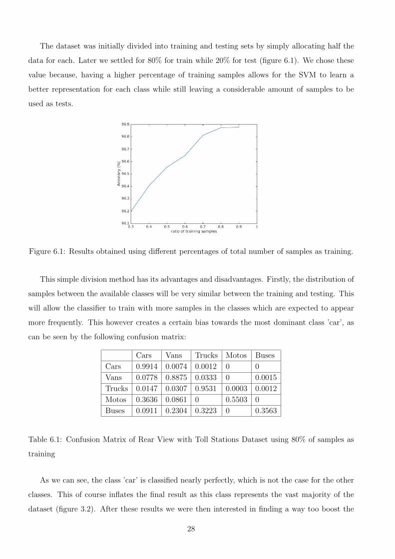
The dataset was initially divided into training and testing sets by simply allocating half the
data for each. Later we settled for 80% for train while 20% for test (figure 6.1). We chose these
value because, having a higher percentage of training samples allows for the SVM to learn a
better representation for each class while still leaving a considerable amount of samples to be
used as tests.
Figure 6.1: Results obtained using different percentages of total number of samples as training.
This simple division method has its advantages and disadvantages. Firstly, the distribution of
samples between the available classes will be very similar between the training and testing. This
will allow the classifier to train with more samples in the classes which are expected to appear
more frequently. This however creates a certain bias towards the most dominant class ’car’, as
can be seen by the following confusion matrix:
Cars Vans Trucks Motos Buses
Cars 0.9914 0.0074 0.0012 0 0
Vans 0.0778 0.8875 0.0333 0 0.0015
Trucks 0.0147 0.0307 0.9531 0.0003 0.0012
Motos 0.3636 0.0861 0 0.5503 0
Buses 0.0911 0.2304 0.3223 0 0.3563
Table 6.1: Confusion Matrix of Rear View with Toll Stations Dataset using 80% of samples as
training
As we can see, the class ’car’ is classified nearly perfectly, which is not the case for the other
classes. This of course inflates the final result as this class represents the vast majority of the
dataset (figure 3.2). After these results we were then interested in finding a way too boost the
28

performance of other classes, even at the expense of a slight decrease in the dominant class.
To achieve this we decided to change the method we used to divided the samples into training
and testing. Our goal was to achieve a far more balanced distribution between the classes in
the training stage. We chose to test two different distributions for the training samples. The
first was simply one third of samples being from the ’car’ class, one third being from the ’van’
class and the remaining third for the ’truck’ class. The second still kept a slight bias towards the
dominant ’car’ class and had the following distribution: half the samples are ofthe class ’cars’
and the other half would be ’vans’ and ’trucks’, one quarter each. We omitted the ’motos’ and
’buses’ classes as they have too few samples to attempt to achieve any significant change. We did
however decide to allocate 90% of the total ’motos’ and ’buses’ samples to training to see if there
were any changes. We also had to reduce our ratio of samples for training as we are limited by
the number of samples of the ’vans’ and ’trucks’ classes. A ratio of 0.3 for the training samples
was used.
Cars Vans Trucks Motos Buses
Cars 0.9646 0.0310 0.0043 0.0002 0.0000
Vans 0.0324 0.9338 0.0317 0.0003 0.0019
Trucks 0.0052 0.0388 0.9532 0.0012 0.0016
Motos 0.1375 0.0900 0.0175 0.7550 0.0000
Buses 0.0229 0.1971 0.2171 0.0000 0.5629
Table 6.2: Confusion Matrix with equal distribution of classes in the training samples.
Cars Vans Trucks Motos Buses
Cars 0.9784 0.0188 0.0026 0.0001 0
Vans 0.0490 0.9169 0.0317 0.0002 0.0023
Trucks 0.0096 0.0390 0.9487 0.0010 0.0017
Motos 0.2000 0.0925 0.0075 0.7000 0
Buses 0.0329 0.1743 0.1857 0 0.6071
Table 6.3: Confusion Matrix with slightly bias distribution of classes in the training samples.
Both tested had somewhat expected results (tables 6.2, 6.3). On both, the classification of the
’car’ class was more error prone whereas the performance of the ’van’ class increased. The ’truck’
class had negligible changes The one that had an equal distribution of classes in the testing set
had a bigger increase in ’van’ classification and a bigger decrease in ’car’ classification. The other
29

distribution had smaller changes however still relevant. Both had a better overall classification
than the previous method for a 0.3 ratio of training samples, and were similar to those obtained
when using a 0.8 ratio using only less than half the samples. We opted to using the second
distribution as it doesn’t require as many samples of ’vans’ and ’trucks’ and allowed us to increase
the ratio of training samples to 0.4. This meant we were able to use more training samples which
allowed us to obtain even better results (table 6.4) and for this reason, for this dataset results
will be presented using this division method of samples between training and testing.
Cars Vans Trucks Motos Buses
Cars 0.9832 0.0165 0.0003 0 0
Vans 0.0402 0.9371 0.0188 0 0.0039
Trucks 0.0040 0.0147 0.9787 0.0004 0.0023
Motos 0.0792 0.0837 0.0563 0.7808 0
Buses 0.0247 0.1775 0.1957 0 0.6021
Table 6.4: Confusion Matrix with slightly bias distribution of classes in the training samples and
a 0.4 ratio.
6.1.1.2 Local HOG descriptors
Figure 6.2: Image showing the different sections of the image used to train the different classifiers.
So far we were simply extracting the global HOG descriptors for the entire image and training
one single classifier in order to do the classification. Here we tested the possibility of training
more than one classifier and using their combined results to boost performance.
Having the classifiers return probability estimates provides greater flexibility when combining
30

the results of the multiple classifiers. In order to do this we made use of Platt’s Scaling [30]
which allowed us to transform SVM output into probabilities estimates using logistic regres-
sion. The image was then divided into six regular sections (figure 6.2) and for each, local HOG
descriptors were extracted and used to train a different SVM. A seventh classifier was trained
with the global HOG features as was being done so far, which we will refer to as main classifier.
Each classifier contributed to the final result with their estimates multiplied by a constant weight.
Individually each classifier presented very distinctive results (table 6.33), ranging from 80%
to 93%. In our first approach we gave each of the first six classifiers the same weight towards
the determination of the final result. This is of course problematic because of the wide range
of individual performances. In an attempt to counter this we gave the main classifier a weight
2.5 times greater than the others. Our goal was to provide the system with more information
so that it could deal with situations where the global HOG descriptor was unsure on the correct
classification.
Classifier Individual Accuracy
1 82%
2 89%
3 92%
4 80%
5 92%
6 93%
7 96,5%
Table 6.5: Individual Classifiers Accuracy.
Cars Vans Trucks Motos Buses
Cars 0.9986 0.0013 0.0001 0.0000 0.0000
Vans 0.1862 0.7912 0.0226 0.0000 0.0000
Trucks 0.0393 0.0211 0.9394 0.0000 0.0001
Motos 0.7124 0.0867 0.0002 0.2007 0.0000
Buses 0.0384 0.1211 0.7148 0.0000 0.1257
Table 6.6: Confusion Matrix using the multiple classifiers for different sections in the image for
the Rear View with Toll Stations Dataset.
By analysing the confusion matrix for this method we easily conclude that the misclassi-
31

fication of other class as ’cars’ greatly increased and the correct classification of cars is close
to perfect. The classifiers that were trained with only part of the image didn’t have as much
discriminatory information and then built an even stronger bias towards the dominant class.
Whenever this classifiers were unsure, they would always default to the most probable result
according to their training, the class ’car’. Additionally both the less represented classes of ’mo-
tos’ and ’buses’ suffered from decrease performance, but for different reasons. The ’motos’ class,
being a smaller vehicle was not well represent in all sections of the image, which made individ-
ual classifiers unable to distinguish this class. On the other hand, although ’buses’ appeared in
all sections, the information in individual sections shared a big resemblance with other classes,
especially the ’trucks’ classes. This meant it was often confused as the ’truck’ class had far more
available samples for training and was better represented.
6.1.1.3 PHOG descriptors
The PHOG descriptor workflow of the system followed a similar path to that of the global HOG
descriptor. PHOG descriptors are extracted for using the entire image and a SVM classifier is
trained using this data.
Cars Vans Trucks Motos Buses
Cars 0.9598 0.0308 0.0078 0.0004 0.0011
Vans 0.0622 0.8871 0.0459 0.0005 0.0043
Trucks 0.0242 0.0461 0.9236 0.0010 0.0051
Motos 0.2833 0.1667 0.0333 0.5167 0
Buses 0.1000 0.1250 0.3000 0 0.4750
Table 6.7: Confusion Matrix obtained using PHOG descriptors on original images of the Rear
View with Toll Stations Dataset.
The descriptor was unable to extract enough descriminatory information for the few ’motos’
and ’buses’ classes samples with both being classified correctly only around 50% of the time. For
all the other classes the results were also slightly worse than those obtained when global HOG
descriptors were used.
32

6.1.2 Segmented Images
So far, the images in the dataset had suffered no preprocessing before the extraction of the HOG
features. As we can see in the images displayed in figure 3.1, this meant that a lot of background
was included in our description of the image. In order to limit this we used the license plates
localization to extract a region of interest (ROI) focusing on the rear of the vehicles (figure 6.3)
a window of 240x180 was used. The localization of the license plate was provided to us by Brisa
since their system captures this information, however it often fails to correctly recognize the
correct location. Therefore we used only the portion of the dataset where the correct location
was detected leaving a total of: 7217 vehicles; 5806 cars; 747 vans; 618 trucks; 8 motos; 38 buses.
Figure 6.3: Rear View with Toll Stations images samples after segmentation
6.1.2.1 Global HOG descriptor
We tested using global HOG descriptors on these segmented images. We also normalized the
distribution of classes in the training samples using the ratios: 50% ’car’, 25% ’van’ and 25%
’truck’. The classes ’motos’ and ’buses’ suffered the same treatment as previously where 90%
of these classes samples were allocated to the training stage. Due to the low amount of ’vans’
and ’trucks’ samples only 30% of the total samples were used for training when using segmented
images.
Comparing with the results obtained in the same circumstances using unsegmented images
(table 6.3) we see that while both the class ’vans’ and ’trucks’ suffered no change, however there
was a 2% increase in the ’car’ class. This was the recorded approximate loss when we normalized
33

Figure 6.4: Rear View with Toll Stations Dataset class distribution using correct license plate
location.
Cars Vans Trucks Motos Buses
Cars 0.9910 0.0084 0.0006 0 0
Vans 0.0446 0.9171 0.0383 0 0.0034
Trucks 0.0115 0.0390 0.9496 0 0.0004
Motos 0.1250 0.1500 0 0.7250 0
Buses 0.0100 0.0800 0.3600 0 0.5500
Table 6.8: Confusion Matrix using global HOG descriptors segmented images of the Rear View
with Toll Stations Dataset.
the training class distribution.
6.1.2.2 Local HOG descriptor
We were interested in seeing how local HOG descriptors would behave when used with segmented
images. Our hypothesis was that by having the segmented images, every single section would
have more relevant information within it, unlike previously where same sections would sometimes
be mainly composed of background.
Overall, there was less disparity between the performance of individual classifiers. As pre-
dicted, relevant information was much better distributed between the different sections, however
34

Classifier Individual Accuracy
1 87%
2 89%
3 89%
4 88%
5 90%
6 92%
7 97%
Table 6.9: Individual Classifiers Accuracy
there was still not enough discriminatory information to achieve high individual levels of accu-
racy. Additionally, despite achieving slightly better results, the main classifier was more often
not confident in its output (30% more samples in which it was not confident) which made the
influence of individual classifiers more noticeable in the final result.
Cars Vans Trucks Motos Buses
Cars 0.9988 0.0012 0.0000 0.0000 0.0000
Vans 0.1902 0.7836 0.0171 0.0000 0.0091
Trucks 0.0453 0.0234 0.9170 0.0000 0.0143
Motos 0.4810 0.0869 0.1321 0.3000 0.0000
Buses 0.0000 0.2640 0.4812 0.0000 0.2548
Table 6.10: Confusion Matrix using the multiple classifiers for different sections in the image for
the segmented Rear View with Toll Stations Dataset.
Individual classifiers still didn’t have access to very discriminatory information which, as can
be seen in the confusion matrix (table 6.10), meant the system tended to default to the most
dominant class. This meant a very good classification of the ’car’ class at the expense of a very
high misclassification rate of other classes as ’cars’.
6.1.2.3 PHOG descriptor
Using PHOG descriptors the system still struggled to distinguish between vans and the other
two classes. A great number of vans were misclassified as either cars or trucks while many trucks
were also misclassified as vans indicating that a good separation between this two classes was
not achieved using this descriptor. Segmenting the image didn’t improve the classification of the
35
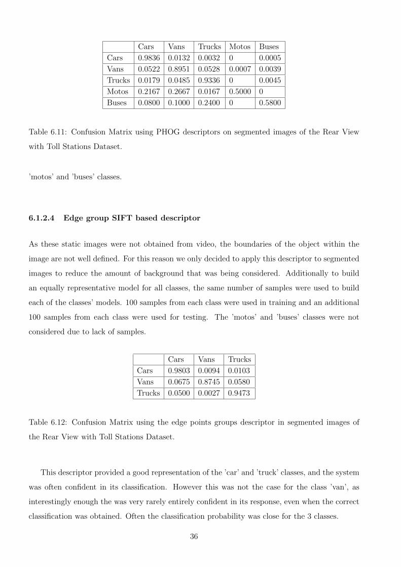
Cars Vans Trucks Motos Buses
Cars 0.9836 0.0132 0.0032 0 0.0005
Vans 0.0522 0.8951 0.0528 0.0007 0.0039
Trucks 0.0179 0.0485 0.9336 0 0.0045
Motos 0.2167 0.2667 0.0167 0.5000 0
Buses 0.0800 0.1000 0.2400 0 0.5800
Table 6.11: Confusion Matrix using PHOG descriptors on segmented images of the Rear View
with Toll Stations Dataset.
’motos’ and ’buses’ classes.
6.1.2.4 Edge group SIFT based descriptor
As these static images were not obtained from video, the boundaries of the object within the
image are not well defined. For this reason we only decided to apply this descriptor to segmented
images to reduce the amount of background that was being considered. Additionally to build
an equally representative model for all classes, the same number of samples were used to build
each of the classes’ models. 100 samples from each class were used in training and an additional
100 samples from each class were used for testing. The ’motos’ and ’buses’ classes were not
considered due to lack of samples.
Cars Vans Trucks
Cars 0.9803 0.0094 0.0103
Vans 0.0675 0.8745 0.0580
Trucks 0.0500 0.0027 0.9473
Table 6.12: Confusion Matrix using the edge points groups descriptor in segmented images of
the Rear View with Toll Stations Dataset.
This descriptor provided a good representation of the ’car’ and ’truck’ classes, and the system
was often confident in its classification. However this was not the case for the class ’van’, as
interestingly enough the was very rarely entirely confident in its response, even when the correct
classification was obtained. Often the classification probability was close for the 3 classes.
36

6.1.3 Comparative Evaluation and discussion
As can be seen by the graphs in figures 6.5, 6.6 all descriptors behaved similarly in the sense
that the class car had the most accurate classification. The biggest difference was that when
the system used local HOG descriptors it struggled to correctly classify vehicles as vans. Apart
from the global HOG descriptor, every single descriptor was unable to generate a descrimina-
tory representation of the class ’motos’ and ’buses’ from the small amount of samples available,
especially the local HOG descriptors.
Figure 6.5: Graph comparing the performances of the system using the different descriptors on
the original unsegmented images.
6.2 Rear View Multi-Lane Free Flow
In this dataset, since we had not only more standardized but also higher resolution images, we
were expecting to achieve better results. However we were also cautious about the lower amount
of samples when compared with the other rear view dataset. In the first test we conducted
we used all the images, both those taken during the day and night. The only exception was
that we didn’t feel it was necessary to use the samples of buses and motos since it was already
demonstrated that this low amount of samples (figure 3.4) aren’t enough to achieve any significant
results.
37
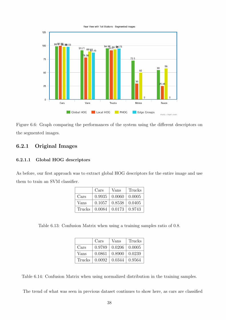
Figure 6.6: Graph comparing the performances of the system using the different descriptors on
the segmented images.
6.2.1 Original Images
6.2.1.1 Global HOG descriptors
As before, our first approach was to extract global HOG descriptors for the entire image and use
them to train an SVM classifier.
Cars Vans Trucks
Cars 0.9935 0.0060 0.0005
Vans 0.1057 0.8538 0.0405
Trucks 0.0084 0.0173 0.9743
Table 6.13: Confusion Matrix when using a training samples ratio of 0.8.
Cars Vans Trucks
Cars 0.9789 0.0206 0.0005
Vans 0.0861 0.8900 0.0239
Trucks 0.0092 0.0344 0.9564
Table 6.14: Confusion Matrix when using normalized distribution in the training samples.
The trend of what was seen in previous dataset continues to show here, as cars are classified
38

with a very accuracy while vans struggle, even after adjusting the attempting to adjust the
distribution of training samples amongst the classes. Testing binary classifications (only using
samples from two classes at a time) we were able to determine that the biggest difficulty was
distinguishing between cars and vans (table 6.15). ’Cars’ vs ’Trucks’ obtained an almost perfect
score and ’vans’ vs ’trucks’ achieve a respectable result of around 97% classification for both
classes.
Cars Vans
Cars 0.9905 0.0095
Vans 0.1124 0.8876
Table 6.15: Confusion Matrix ’Cars’ vs ’Vans’.
In order to determine just how much the low quality night images were influencing the results
we decided to separate our dataset into ’day’ and ’night’. Of the 2068 images 1227 images on
the day set remain.
Cars Vans Trucks
Cars 0.9784 0.0204 0.0012
Vans 0.0682 0.9118 0.0200
Trucks 0.0049 0.0345 0.9636
Table 6.16: Confusion Matrix when using only day images
Results improved as expect, but perhaps not as much as expected. The most affected class
was ’vans’ that registered an improvement of 2%. Other classes weren’t as affected. As can
be seen in figure 3.3, the rear of the vehicle is still visible, even in these night images. The
most important information that is lost is the length of the vehicle which is important when
distinguishing between cars and vans. As can be noted the number of misclassifications of ’vans’
as ’cars’ decreased.
For the other descriptors the system was tested using only day images.
6.2.1.2 Local HOG descriptors
Due to the high width of the images, some sections of the image contained only background. For
this reason we didn’t use this type of descriptors for the original images of this dataset. It will
be used for the segmented images.
39

6.2.1.3 PHOG descriptors
Cars Vans Trucks
Cars 0.9653 0.0287 0.0060
Vans 0.1163 0.8469 0.0367
Trucks 0.0136 0.0300 0.9564
Table 6.17: Confusion Matrix using PHOG descriptor on segmented images of the Front View
Dataset.
The system was not as capable of recognising vehicles as ’vans’ when using PHOG descriptors
when compared to when using global HOG descriptors. PHOG descriptors don’t capture as much
detail of the image as the global HOG.
6.2.2 Segmented Images
Since these images were also provided to us by Brisa, the license plate location was part of the
information we had access to therefore we were able extract a ROI of the images easily following
a procedure similar to that described in section 6.1. With these changes we obtained a far clearer
view of the rear of vehicles when compared to the dataset where toll stations where present. Only
day images were used.
Figure 6.7: Samples of segmented images from Rear View Multi-lane Free Flow Dataset.
40

6.2.2.1 Global HOG descriptors
Global HOG features were extracted using the segmented images. For training, 50% of the
samples were used and the distribution of classes was normalized to: 50% cars, 25% vans and
25% trucks.
Cars Vans Trucks
Cars 0.9895 0.0070 0.0034
Vans 0.0393 0.9396 0.0211
Trucks 0.0003 0.0096 0.9901
Table 6.18: Confusion Matrix using global HOG descriptor on segmented images of Rear View
Multilane Free Flow Dataset.
With this change we were able to increase overall performance. Both trucks and ’vans’ classes
registered an improvement of almost 3% . There was even a slight increase in ’car’ classification.
The information in the background is not rich in relevant information and was not contributing
to the differentiation of the vehicles. Also, as the images were of higher resolution, even after
segmentation the remaining image still retained a great number of detail.
6.2.2.2 Local HOG descriptors
Figure 6.8: Sections in segmented image of the Rear View Multi-lane Free Flow Dataset.
41

Since our segmented images have little background and the vehicles are well standardized
within the image they provide an ideal condition to test the method using local HOG descriptors.
Every section of the image contains important and relevant information of the vehicle (figure 6.8)
which boosted the individual classifiers performance (table 6.19).
Classifier Individual Accuracy
1 95%
2 96%
3 94%
4 95%
5 95%
6 95%
7 98%
Table 6.19: Individual Classifiers Accuracy.
Cars Vans Trucks
Cars 0.9920 0.0035 0.0045
Vans 0.0495 0.9302 0.0202
Trucks 0.0039 0.0021 0.9940
Table 6.20: Confusion Matrix using the multiple classifiers for different sections in the image for
the segmented Rear View Multi-lane Free Flow Dataset.
Case 1 51.83%
Case 2 14.96%
Case 3 20.82%
Case 4 11.89%
Case 5 0.50%
Table 6.21: Behaviour of final results when the classifier’s confidence was below 0.65.
As expected the individual classifiers overall performance is much higher than before. This
means we can have more confidence in their results and we therefore lowered the strength of our
main classifier’s vote from 2.5x to 1.5x. We were interested in analysing the behaviour of the
system when the main classifier was not confident in its output. In order to do this, every time
the main classifier had a probability estimate of 65% or lower on its result we checked to see the
behaviour of the system. There are five possible scenarios:
42

1 - Both the main classifier and the final output of the system are correct. Correctly didn’t
change the correct classification.
2 - The main classifier is incorrect and the final system output shares the same label. Didn’t
change a wrong classification.
3 - The main classifier is incorrect but the final output of the system is correct. Correctly
changed a wrong classification into the correct one.
4 - Both the main classifier and the final output of the system are wrong but don’t share the
same label. Changed a wrong classification into another wrong classification.
5 - The main classifier is correct but the final output of the system is not. Changed the
correct classification into a wrong classification.
Possibilities 1,2,5 have no effect on the overall performance of the system while possibility 3
increases performance and 5 decreases it. As we can see in table 6.33, successful changes are
more prevalent than unsuccessful ones. This means overall, the system performed better than
how it performs with only global HOG descriptors. Looking at the confusion matrix (table 6.20)
we see that while the ’van’ classification is still classified less accurately, however both the ’cars’
and ’trucks’ classes are almost perfectly classified.
6.2.2.3 PHOG descriptor
Cars Vans Trucks
Cars 0.9876 0.0084 0.0039
Vans 0.0593 0.9202 0.0205
Trucks 0.0074 0.0187 0.9739
Table 6.22: Confusion Matrix using PHOG descriptors on segmented images from Rear View
Multi-lane Free Flow Dataset.
The system was able to still achieve a high performance when using PHOG descriptors. The
system shared a similar performance as when using other descriptors in the sense that despite
performing well, the class ’van’ performed poorer when compared to the other classes.
43

6.2.2.4 Edge group SIFT based descriptor
This method was proposed as a solution for vehicle classification in low resolution surveillance
images. In these conditions it achieved good results, however in this dataset the available images
are very different (1392x1040 resolution).
Cars Vans Trucks
Cars 0.9667 0.0167 0.0164
Vans 0.1833 0.8003 0.0164
Trucks 0.0633 0.0200 0.9167
Table 6.23: Confusion Matrix using Edge based SIFT
This method used only edges points as possible keypoints in the image as in low resolution
images they represent the most repeatable and stable features. In higher resolution images, there
are many details that don’t necessarily fall on image edges. In that regard, this method is limiting
and isn’t taking advantage of all the possible information, which results in lower performance
when compared to other methods.
6.2.3 Comparative Evaluation and discussion
Finally
Figure 6.9: Results obtained using different percentages of total number of samples as training
44
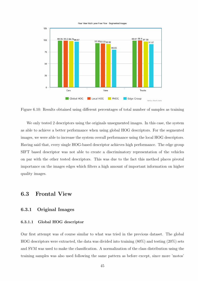
Figure 6.10: Results obtained using different percentages of total number of samples as training
We only tested 2 descriptors using the originals unsegmented images. In this case, the system
as able to achieve a better performance when using global HOG descriptors. For the segmented
images, we were able to increase the system overall performance using the local HOG descriptors.
Having said that, every single HOG-based descriptor achieves high performance. The edge group
SIFT based descriptor was not able to create a discriminatory representation of the vehicles
on par with the other tested descriptors. This was due to the fact this method places pivotal
importance on the images edges which filters a high amount of important information on higher
quality images.
6.3 Frontal View
6.3.1 Original Images
6.3.1.1 Global HOG descriptor
Our first attempt was of course similar to what was tried in the previous dataset. The global
HOG descriptors were extracted, the data was divided into training (80%) and testing (20%) sets
and SVM was used to make the classification. A normalization of the class distribution using the
training samples was also used following the same pattern as before except, since more ’motos’
45

and ’buses’ samples are available, only 60% of these classes’ samples were allocated to training.
Additionally, as more ’vans’ and ’trucks’ samples were available, a ratio of training samples of
0.5 was used.
Cars Vans Trucks Motos Buses
Cars 0.9897 0.0099 0.0002 0 0.0001
Vans 0.0491 0.9165 0.0303 0.0018 0.0023
Trucks 0.0001 0.0121 0.9878 0 0
Motos 0 0.0161 0.0157 0.9682 0
Buses 0 0.0109 0.0347 0 0.9544
Table 6.24: Confusion Matrix of Front View Dataset using 80% of samples as training.
Cars Vans Trucks Motos Buses
Cars 0.9792 0.0197 0.0006 0.0001 0.0004
Vans 0.0415 0.9292 0.0257 0.0015 0.0022
Trucks 0.0004 0.0132 0.9858 0.0006 0
Motos 0 0.0169 0.0173 0.9658 0
Buses 0.0002 0.0113 0.0330 0 0.9554
Table 6.25: Confusion Matrix of Front View Dataset using normalization of training samples
distribution using 50% of the dataset as training samples.
’Cars, ’trucks’, ’motos’ and ’buses’ classes tend to be classified accurately classified, however
vans continue to present less optimal results. One definite conclusion that can be extracted is
that it was indeed the lack of samples for the ’motos’ and ’buses’ classes that was hindering
successful classification. Even a small increase (figure 3.6) in the percentage of samples lead to
great improvement. Another thing we noted is that, unlike previously, trying to normalize the
distribution of samples from each class in training, doesn’t lead to significant improvements. As
all classes already had considerably high performance in the first place, this change only really
affected the ’van’ class that did show some improvement, however the decrease in performance
of the ’car’ class counterbalances this change.
6.3.1.2 Local HOG descriptors
To test the effective of local HOG descriptors we used the same method as the one used in the
previous dataset. The image was divided into six regular sections (figure 6.11), the local HOG
46
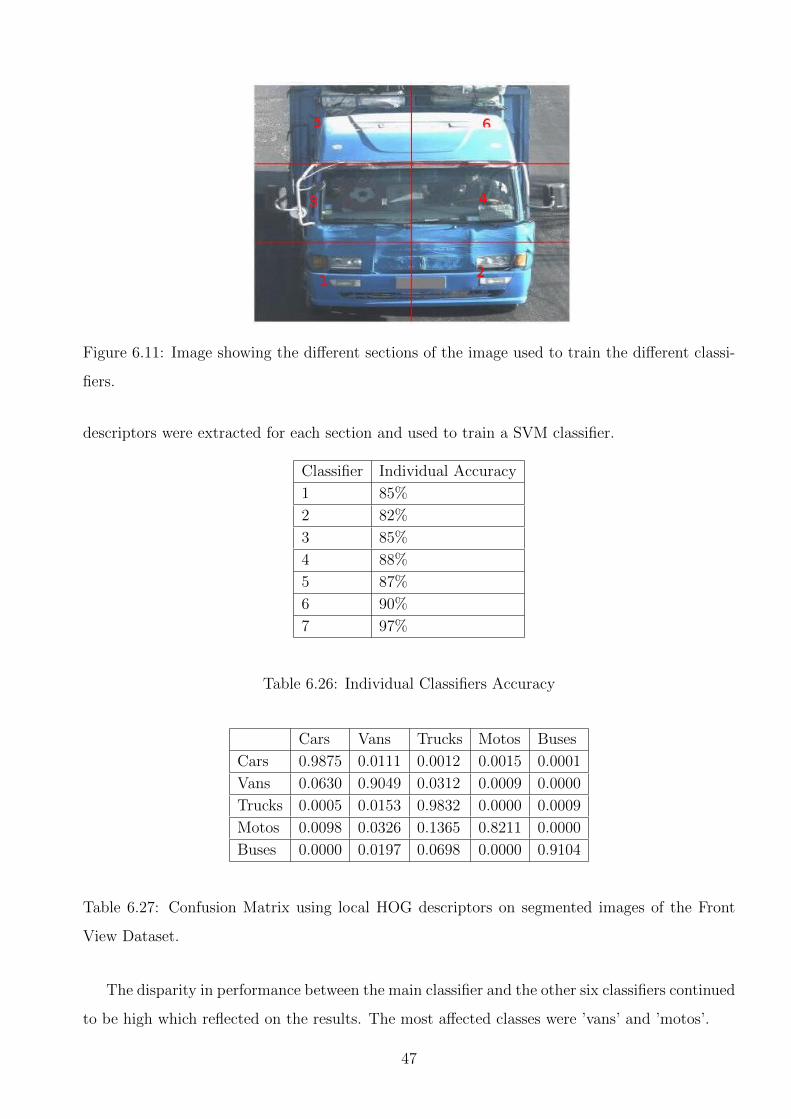
Figure 6.11: Image showing the different sections of the image used to train the different classi-
fiers.
descriptors were extracted for each section and used to train a SVM classifier.
Classifier Individual Accuracy
1 85%
2 82%
3 85%
4 88%
5 87%
6 90%
7 97%
Table 6.26: Individual Classifiers Accuracy
Cars Vans Trucks Motos Buses
Cars 0.9875 0.0111 0.0012 0.0015 0.0001
Vans 0.0630 0.9049 0.0312 0.0009 0.0000
Trucks 0.0005 0.0153 0.9832 0.0000 0.0009
Motos 0.0098 0.0326 0.1365 0.8211 0.0000
Buses 0.0000 0.0197 0.0698 0.0000 0.9104
Table 6.27: Confusion Matrix using local HOG descriptors on segmented images of the Front
View Dataset.
The disparity in performance between the main classifier and the other six classifiers continued
to be high which reflected on the results. The most affected classes were ’vans’ and ’motos’.
47
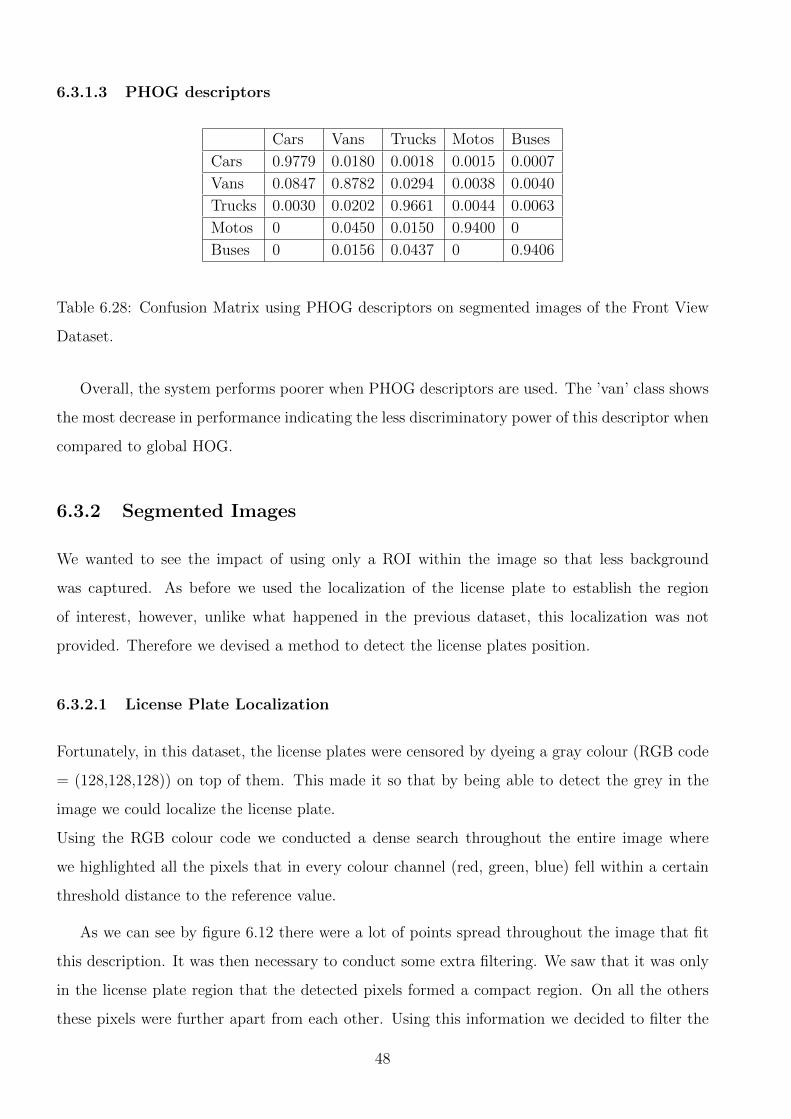
6.3.1.3 PHOG descriptors
Cars Vans Trucks Motos Buses
Cars 0.9779 0.0180 0.0018 0.0015 0.0007
Vans 0.0847 0.8782 0.0294 0.0038 0.0040
Trucks 0.0030 0.0202 0.9661 0.0044 0.0063
Motos 0 0.0450 0.0150 0.9400 0
Buses 0 0.0156 0.0437 0 0.9406
Table 6.28: Confusion Matrix using PHOG descriptors on segmented images of the Front View
Dataset.
Overall, the system performs poorer when PHOG descriptors are used. The ’van’ class shows
the most decrease in performance indicating the less discriminatory power of this descriptor when
compared to global HOG.
6.3.2 Segmented Images
We wanted to see the impact of using only a ROI within the image so that less background
was captured. As before we used the localization of the license plate to establish the region
of interest, however, unlike what happened in the previous dataset, this localization was not
provided. Therefore we devised a method to detect the license plates position.
6.3.2.1 License Plate Localization
Fortunately, in this dataset, the license plates were censored by dyeing a gray colour (RGB code
= (128,128,128)) on top of them. This made it so that by being able to detect the grey in the
image we could localize the license plate.
Using the RGB colour code we conducted a dense search throughout the entire image where
we highlighted all the pixels that in every colour channel (red, green, blue) fell within a certain
threshold distance to the reference value.
As we can see by figure 6.12 there were a lot of points spread throughout the image that fit
this description. It was then necessary to conduct some extra filtering. We saw that it was only
in the license plate region that the detected pixels formed a compact region. On all the others
these pixels were further apart from each other. Using this information we decided to filter the
48

Figure 6.12: All pixels within the threshold of the reference value.
pixels based on their proximity to other pixels that fit the colour criteria. We checked all these
matches and filtered all those that did not have matches in a 2 pixels range in all directions.
Only those that were completely surrounded my matches ended up being chosen and most of
the time this was enough to leave only the region of the license plate. However, in some cases a
few scattered pixels would also pass this second filter. These lingering points outside the license
plate region were filtered by calculating their distance to the median of the remaining points. If
it was above a certain threshold, they would be filtered (Figure 6.13).
Figure 6.13: Pixels remaining after applying filter.
Having the location of the license plate we used it as reference to extract a region of interest
around it. Examples of this image can be seen at (figure 6.14).
49

Figure 6.14: Frontal View dataset images samples after segmentation.
6.3.2.2 Global HOG descriptor
Cars Vans Trucks Motos Buses
Cars 0.9808 0.0158 0.0029 0.0001 0.0004
Vans 0.0611 0.9087 0.0274 0.0008 0.0020
Trucks 0.0038 0.0088 0.9866 0.0006 0.0002
Motos 0.0210 0.0109 0.0047 0.9633 0
Buses 0.0045 0.0067 0.0387 0 0.9501
Table 6.29: Confusion Matrix using global HOG descriptors segmented images of the Front View
Dataset
Comparing the results obtained (table 6.27) with those obtained using the original images
(tables 6.24 and 6.25) we can see that there are no significant changes. One reason why this
change didn’t affect classification as strongly as it did in the previous dataset is that the original
images in this dataset had not only less background present, but also the background was much
less constant throughout different images. On the ”Rear View with Toll Stations” dataset, all
images were taken in just a few different spaces (images from a total of nine cameras were used),
whereas that doesn’t seem to be the case in this dataset. This means that background plays a
much lesser part on the classification process and therefore, filtering it through segmentation as
a much lesser impact.
50

6.3.2.3 Local HOG descriptors
When applying the same regular division of the image into six sections we saw that there wasn’t
much improvement on the performance of the individual classifiers which resulted in slightly
worse results when compared to using only global HOG descriptors (table 6.30).
Cars Vans Trucks Motos Buses
Cars 0.9786 0.0182 0.0026 0.0005 0.0001
Vans 0.0716 0.8968 0.0304 0 0.0011
Trucks 0.0083 0.0134 0.9779 0.0005 0
Motos 0 0.0665 0.0432 0.8903 0
Buses 0.0051 0.0103 0.0570 0 0.9276
Table 6.30: Confusion Matrix using local HOG descriptors on segmented images of the Front
View Dataset with regular division.
For this reason we decided to test an irregular division focusing on specific well defined
sections of the vehicle, namely the lights and the front mirror. We used the three different
sections displayed in figure 6.15. As before, an additional classifier was trained using global
HOG descriptors.
Figure 6.15: Image showing the irregular sections of the image used to train the different classi-
fiers.
Using these different sections we were able to achieve much higher individual classifications
which allowed to increase the overall performance of the system slightly as can be seen in table
6.32. The most improved class was the ’motos’, but both the ’buses’ and ’vans’ classes recorded
some improvement.
51

Classifier Individual Accuracy
1 95%
2 93%
3 95%
4 96.7%
Table 6.31: Individual Classifiers Accuracy.
Cars Vans Trucks Motos Buses
Cars 0.9886 0.0089 0.0024 0.0001 0
Vans 0.0616 0.9168 0.0205 0 0.0011
Trucks 0.0033 0.0084 0.9879 0 0.0005
Motos 0 0.0362 0.0121 0.9516 0
Buses 0.0128 0.0106 0.0296 0 0.9470
Table 6.32: Confusion Matrix using local HOG descriptors on segmented images of the Front
View Dataset with irregular division.
As we did in the previous dataset, we were interested in analysing the behaviour of the system
when the main classifier was not confident, below 65%. We did this by analysing the same five
possibilities as described in 6.2.2.2.
Case 1 47.42%
Case 2 25.77%
Case 3 13.40%
Case 4 13.40%
Case 5 0%
Table 6.33: Behaviour of final results when the classifier’s confidence was below 0.65.
The system didn’t change any correct answers, meaning there was no decrease in performance,
while 13.40% of the time the main classifier was not confident the system was able to change a
wrong classification into the correct one.
6.3.2.4 PHOG
When using segmented images, PHOG descriptors performed more on par with the global HOG
descriptor if only still slightly poorer. The classes ’motos’ and ’buses’ were the most affected as
52

can be seen in the confusion matrix 6.34.
Cars Vans Trucks Motos Buses
Cars 0.9743 0.0206 0.0041 0.0005 0.0005
Vans 0.0771 0.8923 0.0264 0.0011 0.0030
Trucks 0.0050 0.0218 0.9700 0.0017 0.0015
Motos 0 0.0511 0.0252 0.9232 0.0004
Buses 0.0003 0.0107 0.0441 0.0033 0.9416
Table 6.34: Confusion Matrix using PHOG descriptor on segmented images of the Front View
Dataset.
6.3.2.5 Edge group SIFT based descriptor
We used 100 training samples for the ’car’, ’vans’ and ’trucks’ classes, but due to few samples
we only used 50 for both trucks and motos. In the test we used 60 samples for each class except
the ’motos’ class that didn’t have enough samples left. Only 33 ’motos’ samples were used for
the test for this reason.
Cars Vans Trucks Motos Buses
Cars 0.9779 0.0180 0.0018 0.0015 0.0007
Vans 0.0847 0.8782 0.0294 0.0038 0.0040
Trucks 0.0030 0.0202 0.9661 0.0044 0.0063
Motos 0 0.0450 0.0150 0.9400 0
Buses 0 0.0156 0.0437 0 0.9406
Table 6.35: Confusion Matrix using Edge group SIFT based descriptor on segmented images of
the Front View Dataset.
Despite using fewer samples for the creation of the ’motos’ and ’buses’ constellation models,
the system still managed to achieve a reasonable performance when classifying these types of
vehicles. Overall this system performs well considering how different the images are from the
images used in the work where this method was proposed. Apart from the ’van’ class, this system
performs at a similar level to that achieved when using global HOG descriptors.
53
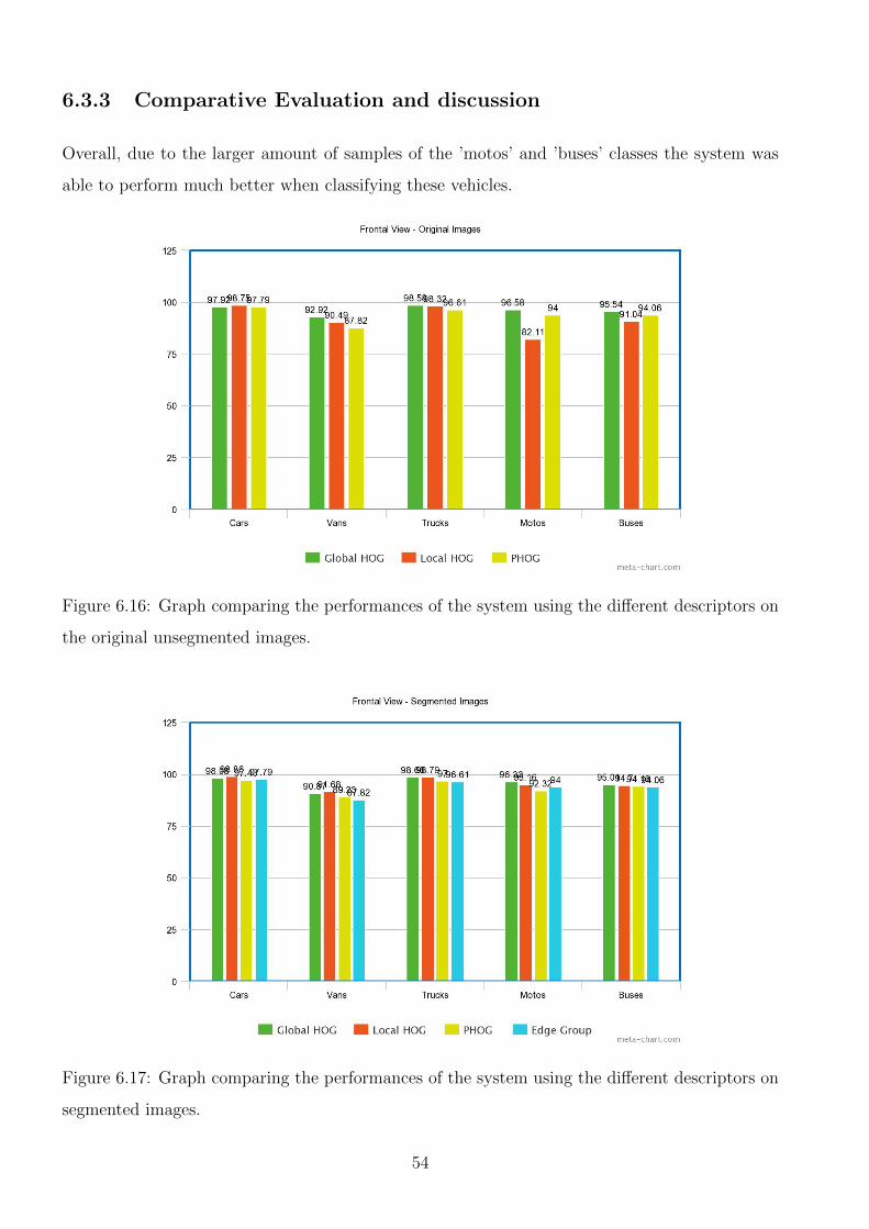
6.3.3 Comparative Evaluation and discussion
Overall, due to the larger amount of samples of the ’motos’ and ’buses’ classes the system was
able to perform much better when classifying these vehicles.
Figure 6.16: Graph comparing the performances of the system using the different descriptors on
the original unsegmented images.
Figure 6.17: Graph comparing the performances of the system using the different descriptors on
segmented images.
54

All descriptors achieved similar results when classifying ’cars’ and ’trucks’. On the other hand
the classes ’vans’ and ’motos’ recorded the biggest discrepancy. By using an irregular division of
the segmented images, we were able to increase the overall system performance using local HOG
descriptors.
6.4 Top Side View
This dataset allowed to test out system when classifying low resolution images from surveillance
cameras. In lower resolution images, fewer details are available and for that reason the system
is not able to achieve the same levels of performance as in previous datasets. Due to the lack of
samples of the classes ’motos’ and ’buses’ we did not attempt to classify these types of vehicles.
6.4.1 Global HOG descriptors
As was the case with the previous datasets we extracted the global HOG descriptors for the
entire image and used a SVM classifier to learn and classify the data. However, because of the
lower resolution images, a smaller 8x8 cell region was used when computing the HOG.
We tested the system both using a standard division of samples between training (80%) and
testing (20%) (table 6.41) and a normalization of the distribution of classes in the training stage
(table 6.40).. In the latter, 30% of the dataset’s sample were used for training and followed the
distribution: 50% - cars; 25% vans; 25% trucks.
Cars Vans Trucks
Cars 0.9828 0.0169 0.0004
Vans 0.1586 0.8000 0.0414
Trucks 0.0073 0.0756 0.9171
Table 6.36: Confusion Matrix using 80% samples for training.
As can be seen by the confusion matrices the low resolution images make it especially hard to
classify ’vans’ as they become more and more similar to ’cars’. Even after attempting to normalize
the distribution of classes in the training samples the class ’van’ saw no significant change while
there was a trade-off between the performances of the truck’ and ’car’ classes. Attempting to
achieve accurate classification with such low quality samples is hard since inter-class variations
55

Cars Vans Trucks
Cars 0.9641 0.0356 0.0003
Vans 0.1335 0.8091 0.0575
Trucks 0.0088 0.0608 0.9304
Table 6.37: Confusion Matrix using normalized distribution of training samples.
begin to be less and less noticeable. In a meeting with Brisa we were informed that the goal for
these types of images is traffic monitoring and surveillance. We were told that these cameras
would be used for vehicle counting, traffic queues detection and that, instead of distinguishing
between classes such as ’vans’, ’cars’ and ’trucks’ they were more interested whether a vehicle
classified as ’heavy’ or ’light’. This meant that the distinction between ’vans’ and ’cars’ would
not necessary as in most cases, they would both belong to the ’Light vehicles’ category. In order
to determine the effectiveness of the classifier in these conditions we distributed the ’van’ class
samples into the ’car’ and ’trucks’ based on their size (figure 6.18). We used 80% of the dataset
for training and 20% for testing.
Figure 6.18: Top Side View Dataset distribution of ’Heavy’ and ’Light’ vehicles.
Light Heavy
Light 0.9840 0.0160
Heavy 0.0268 0.9732
Table 6.38: Confusion Matrix using two broader classes.
As expected, using these broader classes it is possible to achieve very accurate results. For
monitoring and traffic estimation, these classifications errors are within what would be acceptable.
56

6.4.2 Local HOG descriptor
Due to the low resolution of the images, we found no advantages of using this method as there
wasn’t enough discriminatory information in the individual sections (maximum individual accu-
racy of 70%). Some form of boosting of the combined result could be employed, however that
option wasn’t explored in this work.
6.4.3 PHOG descriptor
Cars Vans Trucks
Cars 0.9713 0.0277 0.0010
Vans 0.1578 0.7683 0.0738
Trucks 0.0052 0.1018 0.8929
Table 6.39: Confusion Matrix using PHOG descriptor on Top Side View Dataset images.
Light Heavy
Light 0.9916 0.0084
Heavy 0.0591 0.9409
Table 6.40: Confusion Matrix using PHOG descriptors and two broader classes.
Using PHOG descriptors the system achieved good performance when classifying the ’car’
class, however that was not the case for the other two classes. When classifying between the
’heavy’ and ’light’ classes the performance of the system improved.
6.4.4 Edge group SIFT based descriptor
In this dataset we used the images most similar to the ones used in Ma and Grimson’s original
work [24]. For this reason we were interested in seeing how this method would perform on a
similar setting, even though the vehicle’s view was slightly different.
The results were much lower than those obtained using HOG features. We believed the
classification was hindered because of the vehicle’s masks. As was explained in Chapter 2, the
SIFT features are computed for the vehicles edges. To make sure only the vehicle’s edges are
used and not other edges in the image the mask is used to filter the image edge points. The
57

Cars Vans Trucks
Cars 0.9625 0.0350 0.0025
Vans 0.1200 0.7357 0.1443
Trucks 0.0049 0.0344 0.9607
Table 6.41: Confusion Matrix using edge points groups descriptor
Light Heavy
Light 0.9701 0.0299
Heavy 0.2139 0.7861
Table 6.42: Confusion Matrix using two classes ’heavy’ vs ’light’ filtering edges using an image
mask.
mask we were able to extract using the Gaussian Mixture based background extraction method
explained in Chapter 3 were not perfect as, they often didn’t cover the entire vehicle. This was
acceptable for vehicle detection, however we believe that might be one of the reasons why results
were so low. We decided to remove the mask filter and computed the SIFT features along the
edges of the entire image in order to see whether it would result in improved performance.
Light Heavy
Light 0.9751 0.0249
Heavy 0.1293 0.8707
Table 6.43: Confusion Matrix using two classes ’heavy’ vs ’light’ without filtering edges using an
image mask.
As expected there were some improvements, however they still come short of what was
achieved previously. A more refined background segmentation algorithm or processing the masks
in order to improve their representativeness of the vehicles location could further improve the
results.
58

Chapter 7
Conclusions
Vehicle classification is a fundamental task in automatic tolling systems, surveillance and traffic
monitoring. Throughout this work we developed a system able to accurately distinguish between
up to five different classes of vehicles: ’cars’, ’vans’, ’trucks’, ’motos’, ’buses’. We implement four
different methods. Three used HOG-based descriptors (global HOG, local HOG, and PHOG) in
combination with SVM classifier(s) while the fourth was based on the work of Ma and Grimson
[24] and used edge points group SIFT based descriptors to build constellation models of the dif-
ferent classes. We manually labelled three different datasets containing static images of vehicles.
An additional fourth dataset was created from scratch using videos from surveillance cameras
installed in American motorways. This forth dataset will be made available to be used in similar
projects.
Throughout the course of this project it was possible to reach important conclusions. All meth-
ods tested were able to describe the images in a discriminatory manner allowing the system to
achieve good performance. The system was able to perform consistently well when using global
HOG descriptors, achieving better results than when using PHOG descriptors. Still, we were able
to increase performance by combining the outputs of multiple SVM classifiers trained using local
HOG descriptors. The best results were obtained when the individual results of every classifier
were high, which was possible when discriminatory information was present in different sections
of the image. With higher resolution , highly standardized images (”Rear View Multi-Lane Free
Flow Dataset”), a regular division of the image was enough, however for other types of images
this might not be the case. In this work we used an irregular division of the image focusing
on known features of the vehicle, namely the lights and front mirror (”Frontal View Dataset”),
which allowed the individual classifiers to achieve a high performance. Instead of applying this
59
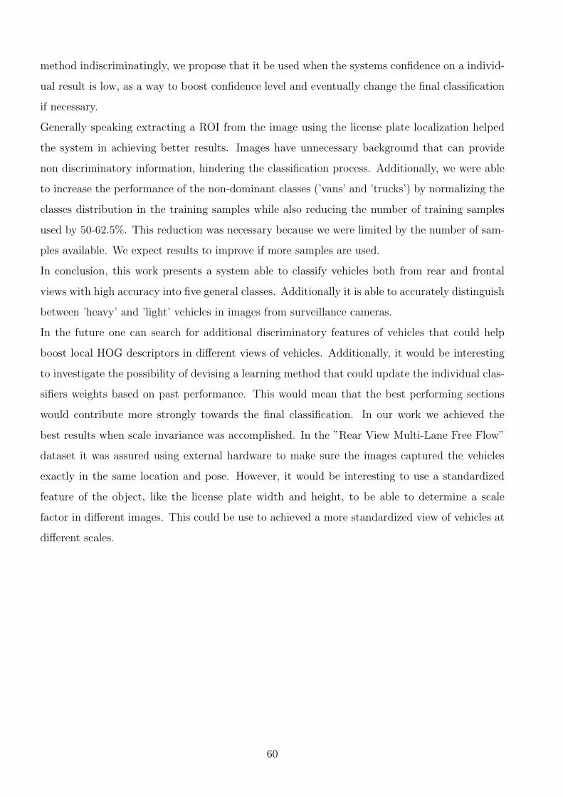
method indiscriminatingly, we propose that it be used when the systems confidence on a individ-
ual result is low, as a way to boost confidence level and eventually change the final classification
if necessary.
Generally speaking extracting a ROI from the image using the license plate localization helped
the system in achieving better results. Images have unnecessary background that can provide
non discriminatory information, hindering the classification process. Additionally, we were able
to increase the performance of the non-dominant classes (’vans’ and ’trucks’) by normalizing the
classes distribution in the training samples while also reducing the number of training samples
used by 50-62.5%. This reduction was necessary because we were limited by the number of sam-
ples available. We expect results to improve if more samples are used.
In conclusion, this work presents a system able to classify vehicles both from rear and frontal
views with high accuracy into five general classes. Additionally it is able to accurately distinguish
between ’heavy’ and ’light’ vehicles in images from surveillance cameras.
In the future one can search for additional discriminatory features of vehicles that could help
boost local HOG descriptors in different views of vehicles. Additionally, it would be interesting
to investigate the possibility of devising a learning method that could update the individual clas-
sifiers weights based on past performance. This would mean that the best performing sections
would contribute more strongly towards the final classification. In our work we achieved the
best results when scale invariance was accomplished. In the ”Rear View Multi-Lane Free Flow”
dataset it was assured using external hardware to make sure the images captured the vehicles
exactly in the same location and pose. However, it would be interesting to use a standardized
feature of the object, like the license plate width and height, to be able to determine a scale
factor in different images. This could be use to achieved a more standardized view of vehicles at
different scales.
60

References
[1] Amol Ambardekar, Mircea Nicolescu, George Bebis, and Monica Nicolescu. Vehicle classifi-
cation framework: a comparative study. EURASIP Journal on Image and Video Processing,
2014(1):1–13, 2014.
[2] Austroads. http://www.austroads.com.au/.
[3] Norbert Buch, Mark Cracknell, James Orwell, and Sergio A Velastin. Vehicle localisation
and classification in urban cctv streams. Proc. 16th ITS WC, pages 1–8, 2009.
[4] John Canny. A computational approach to edge detection. Pattern Analysis and Machine
Intelligence, IEEE Transactions on, (6):679–698, 1986.
[5] Census. http://www.census.gov/compendia/statab/cats/transportation/motor_
vehicle_accidents_and_fatalities.html.
[6] Chih-Chung Chang and Chih-Jen Lin. LIBSVM: A library for support vector machines.
ACM Transactions on Intelligent Systems and Technology, 2:27:1–27:27, 2011. Software
available at http://www.csie.ntu.edu.tw/~cjlin/libsvm.
[7] Zezhi Chen and Tim Ellis. Multi-shape descriptor vehicle classification for urban traffic. In
Digital Image Computing Techniques and Applications (DICTA), 2011 International Con-
ference on, pages 456–461. IEEE, 2011.
[8] Zezhi Chen, Nick Pears, Michael Freeman, and Jim Austin. Road vehicle classification using
support vector machines. In Intelligent Computing and Intelligent Systems, 2009. ICIS 2009.
IEEE International Conference on, volume 4, pages 214–218. IEEE, 2009.
[9] Xavier Clady, Pablo Negri, Maurice Milgram, and Raphael Poulenard. Multi-class vehicle
type recognition system. In Artificial Neural Networks in Pattern Recognition, pages 228–
239. Springer, 2008.
61

[10] David E Clark and Brad M Cushing. Predicted effect of automatic crash notification on
traffic mortality. Accident Analysis & Prevention, 34(4):507–513, 2002.
[11] Michal Conos. Recognition of vehicle make from a frontal view. Master, Czech Tech. Univ.,
Prague, Czech Republic, 2006.
[12] Navneet Dalal and Bill Triggs. Histograms of oriented gradients for human detection. In
Computer Vision and Pattern Recognition, 2005. CVPR 2005. IEEE Computer Society Con-
ference on, volume 1, pages 886–893. IEEE, 2005.
[13] BASSAM DAYA, Al HUSSAIN AKOUM, and SAMIA BAHLAK. Geometrical features for
multiclass vehicle type recognition using mlp network. Journal of Theoretical & Applied
Information Technology, 43(2), 2012.
[14] Piotr Dollar. Piotr’s Computer Vision Matlab Toolbox (PMT). http://vision.ucsd.edu/
~pdollar/toolbox/doc/index.html.
[15] Zhen Dong and Yunde Jia. Vehicle type classification using distributions of structural and
appearance-based features. In Image Processing (ICIP), 2013 20th IEEE International Con-
ference on, pages 4321–4324. IEEE, 2013.
[16] Zhen Dong, Yuwei Wu, Mingtao Pei, and Yunde Jia. Vehicle type classification using a
semisupervised convolutional neural network.
[17] Kai-Bo Duan, Jagath C Rajapakse, and Minh N Nguyen. One-versus-one and one-versus-all
multiclass svm-rfe for gene selection in cancer classification. In Evolutionary Computation,
Machine Learning and Data Mining in Bioinformatics, pages 47–56. Springer, 2007.
[18] Kun Duan, Luca Marchesotti, and David J Crandall. Attribute-based vehicle recognition
using viewpoint-aware multiple instance svms. In Applications of Computer Vision (WACV),
2014 IEEE Winter Conference on, pages 333–338. IEEE, 2014.
[19] Brisa Auto estradas de Portugal S. A. http://www.brisa.pt/.
[20] Robert Fergus, Pietro Perona, and Andrew Zisserman. Object class recognition by un-
supervised scale-invariant learning. In Computer Vision and Pattern Recognition, 2003.
Proceedings. 2003 IEEE Computer Society Conference on, volume 2, pages II–264. IEEE,
2003.
62

[21] Pedro Ferreira, Pedro Jorge, Goncalo Marques, Arnaldo Abrantes, and Antonio Amador.
Integrated vehicle classification system. In Intelligent Vehicles Symposium (IV), 2011 IEEE,
pages 266–271. IEEE, 2011.
[22] R. B. Girshick, P. F. Felzenszwalb, and D. McAllester. Discriminatively trained deformable
part models, release 5. http://people.cs.uchicago.edu/~rbg/latent-release5/.
[23] David G Lowe. Distinctive image features from scale-invariant keypoints. International
journal of computer vision, 60(2):91–110, 2004.
[24] Xiaoxu Ma and W Eric L Grimson. Edge-based rich representation for vehicle classification.
In Computer Vision, 2005. ICCV 2005. Tenth IEEE International Conference on, volume 2,
pages 1185–1192. IEEE, 2005.
[25] Xiang bai Pan chen and Wenyu Liu. Vehicle color recognition on an urban road by feature
context.
[26] Yu Peng, Jesse S Jin, Suhuai Luo, Min Xu, and Yue Cui. Vehicle type classification us-
ing pca with self-clustering. In Multimedia and Expo Workshops (ICMEW), 2012 IEEE
International Conference on, pages 384–389. IEEE, 2012.
[27] Bojan Pepikj, Michael Stark, Peter Gehler, and Bernt Schiele. Multi-view and 3d deformable
part models.
[28] K Person. On lines and planes of closest fit to system of points in space. philiosophical
magazine, 2, 559-572, 1901.
[29] Vladimir S Petrovic and Timothy F Cootes. Analysis of features for rigid structure vehicle
type recognition. In BMVC, pages 1–10, 2004.
[30] John Platt et al. Probabilistic outputs for support vector machines and comparisons to
regularized likelihood methods. Advances in large margin classifiers, 10(3):61–74, 1999.
[31] M Saquib Sarfraz and M Haris Khan. A probabilistic framework for patch based vehicle
type recognition. In VISAPP, pages 358–363, 2011.
[32] Chris Stauffer and W Eric L Grimson. Adaptive background mixture models for real-
time tracking. In Computer Vision and Pattern Recognition, 1999. IEEE Computer Society
Conference on., volume 2. IEEE, 1999.
63

[33] A. Vedaldi and B. Fulkerson. VLFeat: An open and portable library of computer vision
algorithms. http://www.vlfeat.org/, 2008.
[34] European Association with tolled motorways bridges and tunnels. http://www.asecap.
com/.
[35] Wei Xiang, Colin W Otto, and Peng Wen. Automated vehicle classification system using
advanced noise reduction technology. In Proceedings of the 1st International Conference on
Signal Processing and Communication Systems (ICSPCS 2007). DSP for Communication
Systems, 2008.
[36] Bailing Zhang. Reliable classification of vehicle types based on cascade classifier ensembles.
Intelligent Transportation Systems, IEEE Transactions on, 14(1):322–332, 2013.
[37] Chengcui Zhang, Xin Chen, and Wei-bang Chen. A pca-based vehicle classification frame-
work. In Data Engineering Workshops, 2006. Proceedings. 22nd International Conference
on, pages 17–17. IEEE, 2006.
64

Acronyms and symbols
Abbreviation Meaning
ISR Institute of Systems and Robotics
ITS Intelligent Transport System
CCTV Closed-Circuit TeleVision
HOG Histogram of Oriented Histograms
FHOG Felzenszwalb’s Histogram of Oriented Histograms
PHOG Pyramid Histogram of Oriented Histograms
SVM Support Vector Machine
SIFT Scale Invariant Feature Transform
PCA Principal Component Analysis
SUV Sport utility vehicle
MPV Multi-purpose vehicle
LDA Linear Discriminant Analysis
IVCS Integrated Vehicle Classification System
MLFF Multi-Lane Free Flow
AVDC Automatic Vehicle Detection and Classification
ALPR Advance License Plate Recognition
OvO One versus One
OvA One versus All
ROI Region of Interest
65