AARES 52nd ANNUAL CONFERENCE 2008

MULTI-OUTPUT BROADACRE AGRICULTURAL PRODUCTION: ESTIMATING A COST FUNCTION USING QUASI-MICRO FARM LEVEL DATA FROM AUSTRALIA

Duong T. M. Nguyen, Keith McLaren and Xueyan Zhao Department of Econometrics and Business Statistics, Monash University

MULTI-OUTPUT BROADACRE AGRICULTURAL PRODUCTION: ESTIMATING A COST FUNCTION USING QUASI-MICRO FARM LEVEL DATA FROM AUSTRALIA∗

Duong T. M. Nguyen, Keith McLaren and Xueyan Zhao Department of Econometrics and Business Statistics, Monash University ABSTRACT Existing econometric models for Australian broadacre agricultural production are few and have become dated. This paper estimates a multi-product restricted cost function using a unique quasi-micro farm level dataset from the Australian Agricultural and Grazing Industries Survey. Both the transcendental logarithmic and normalized quadratic functional forms are employed. Heteroskedasticity caused by the particular nature of the quasi-micro data is also assessed and accommodated. Allen partial elasticities of input substitution and own-and cross-price input demand elasticities are computed. The estimated demands for most production factors are inelastic to prices. Hired labour is responsive to own price and cropping input prices.

∗ This paper is prepared for the AARES 2008 conference and forms a part of Duong Nguyen’s PhD study conducted at the Department of Econometrics and Business Statistics at Monash University, which is funded by an ARC APA(I) grant with the New South Wales Department of Primary Industries as industry partner. We wish to express our sincere thanks to Prof. John D. Mullen and Prof. Garry Griffith for their insightful comments and suggestions throughout this research. We also would like to thank Walter Shafron and Colin Mues at ABARE for compiling the data used in this study. Contact author: Duong (Dawn) T. M. Nguyen. Email: dawn.nguyen@buseco.monash.edu.au. Phone: (03)9905 8416.

2

TABLE OF CONTENT

1. INTRODUCTION.......................................................................................................3

2. THEORETICAL FRAMEWORK FOR THE RESTRICTED COST FUNCTION ........8

2.1. The cost function ........................................................................................... 8 2.2. The restricted translog cost function ..................................................... 10 2.3. The restricted normalized quadratic cost function ............................ 13

3. DATA ......................................................................................................................14

3.1. The AAGIS Data ............................................................................................ 14 3.2. Specifications of input, output and other exogenous variables ..... 15 3.3. A unique feature of the Data – Adjusting for heteroskedasticity.... 19

4. EMPIRICAL ESTIMATION AND RESULTS...........................................................21

4.1. Econometric estimation and coefficient estimates ............................ 22 4.2. Estimated elasticities ( ijσ and ijη ) ............................................................ 26 4.3. Technology Tests......................................................................................... 28 4.4. Discussion of results .................................................................................. 29

5. CONCLUSION ........................................................................................................30

APPENDIX A: DATA AGGREGATION ..........................................................................32

APPENDIX B: ESTIMATING STANDARD ERRORS USING BOOSTRAPPING..........36

REFERENCES: ..............................................................................................................37

3

1. INTRODUCTION This paper presents an application of duality methods to Australian broadacre production to draw information on input demand decisions. It fills in a notable gap in the literature of econometric models for Australian agricultural production with the estimation of multi-product cost functions using a unique nationwide quasi-micro farm-level dataset. Two commonly used functional forms, transcendental logarithmic and normalized quadratic, are used for comparison purposes. The performance of broadacre production in Australia has a strong influence on the overall economic performance and the vitality and welfare of a vast rural area that supports a significant proportion of the population. The sector has a significant role in international trade with the majority of total broadacre agriculture production exported. It has also constantly evolved with respect to technology, marketing structure and institutional structure to remain internationally competitive. Therefore, knowledge of the underlying production technology and the interrelationships between inputs and outputs at a national level are crucial for policy makers to assist in the sector’s future development and its competitive position in international markets. Over the last few decades, in searching for information on technological relationships in rural production, international researchers have usually applied the duality approach. In this approach, the technological relationships are indirectly extracted through the estimation of the cost, revenue or profit functions using input and output prices rather than the traditional primal production function using the input and output quantities. This methodology assumes farmers to be optimizers, so that they either minimise cost, maximise revenue or maximise profit under technological constraints. Prominent contributions to this field are Hotelling (1932), Shephard (1953), Diewert (1971), Christensen, Jorgenson and Lau (1973), Lau (1974) and McFadden (1978). These papers together establish the theoretical duality between the cost, revenue and profit functions, usually called the dual objective functions, and the primal production function. The duality methods have become widely accepted, not just for their sound theoretically-proven duality but also for several empirical advantages. Firstly, by estimating the objective function analysts are not required to impose linear homogeneity among input and output quantities so any form of relationship between them can be accommodated. Secondly, the variables in econometric models of the objective functions are prices rather than quantities, which appear in the primal production function and over which the farmers have control, so they fit better the exogeneity assumption for robust econometric estimation. Thirdly, the problem of multicollinearity can be alleviated in the estimation of the dual functions compared to the primal function because, at a micro level, input quantities are more likely to move together than their prices. Moreover, with the objective

4

functions, the measures of economic interest, such as price elasticities, can be derived in a relatively simpler fashion. In addition, researchers applying the duality approach can make conclusions about various aspects of the underlying technology. A host of theories and tests have been developed for examining the structure or characteristics of the underlying production technology such as homotheticity, economies of size, increasing/decreasing/constant returns to scale, input and output nonjointness and separability, and bias in technical change via estimating the dual functions. With these relative pros, the applications of duality have gone beyond the boundary of traditional production technology with empirical research such as Lawrence (1989) and Kohli (1994) in international trades or Halvorsen and Smith (1986) in exploitation of unpriced natural resources. A major development in the history of the duality approach was the introduction of flexible functional forms in the early 1970s. These functional forms, such as Generalized Leontief, normalized quadratic and transcendental logarithmic (translog), to name a few, have enough distinct parameters to accommodate interrelationships between inputs and/or outputs without imposing many a priori restrictions on economic behaviour, which is a fundamental advantage over the traditional Cobb-Douglas or CES forms. Their introduction greatly assisted the acceptance of the duality approach in empirical production research. However, after an initial rush of studies embracing this approach, with the use of flexible functional forms, significant empirical issues and problems emerged and have remained unresolved. The most formidable challenges in duality applications are the aggregation problem, the choice of the dual function (whether it is a cost, revenue or profit function) and the choice of functional form. It has been a common and unquestioned practice to use aggregate, national or state average data, normally in time-series form, in dual-based empirical research, which is largely due to unavailability of micro/farm-level data. This conduct, however, raises a few fundamental issues. Duality theory is concerned with microeconomic rather than macroeconomic behaviour and so it is questionable how well aggregate data convey information about individual production units. Liu and Shumway (2004), Shumway and Davis (2001) and Chambers (1988) stressed that the conditions for consistent aggregation across firms are too strict for practical application. To use agent-wise aggregate data, it is a requirement that production units use identical production technology (Polson and Shumway, 1990). In the context of farming, where the technology employed and the operational and climatic conditions are highly heterogeneous across farms, the use of aggregate data can result in misleading research results and thus erroneous policy interpretations (Morrison Paul, 2001). Another limitation of using aggregate data in duality research is estimation bias resulting from simultaneity. In a competitive market, firms have control over what input quantities to be used but not their prices. At an aggregate level, however, price and quantity are

5

simultaneously determined via demand-supply principles. Moreover, it has been suggested that the estimated dual functions’ frequent failure to meet restrictions required to portray rational economic behaviour in past studies is attributable to ignorance of time-series characteristics of aggregate data (Lim and Shumway, 1997). As problematic as the issue of data aggregation is the choice of which dual objective function to employ. In applying duality methods, researchers have a choice to estimate either a cost, revenue or profit function. Theoretically these functions are dual to each other and to the production function. There has been no general guidance for making this choice and this is an empirical matter being shaped by the researcher’s intuitions and purposes, and data availability. The profit function has been favoured over the other two functions because in the estimation of this function the input and output prices, not just input prices or output prices alone, both appear as exogenous variables in the estimation equation(s). This supports the hypothesis that producers take into consideration prices on both the producing and selling sides, not just one of them. This, however, can become an empirical drawback of estimating the profit function because relatively more parameters need to be estimated, putting more pressure on the usually small data samples and necessitating potentially improper data aggregation. Another shortcoming of the profit function, in comparison to the other two dual functions, is that profit is often calculated as the residual difference between the production revenues and production costs. This means that the calculated production profit absorbs any differences in the revenues expected at the time production decisions are made (when costs are incurred) and the revenues realized when outputs are sold. Although care is taken in approximating the revenue expectations in the past estimations of the profit functions, this intertemporal difference is likely to cause data errors. Meanwhile, the cost function has a major advantage over the profit function in allowing for both increasing and decreasing returns to scale to be revealed. In the estimation of the profit function it is implicitly assumed that the technology under consideration displays decreasing returns to scale. In addition to the choice of which among the three dual functions to estimate, empirical researchers also have to make a decision regarding the flexible functional form to use. Flexible forms that have been introduced include translog (Christensen et al. , 1973; Binswanger,1974a; and Ollinger, MacDonald and Madison, 2005), normalized quadratic (Yotopoulos, Lau and Wuu-Long, 1976; Shumway, 1983; and Moschini, 1988), Generalized Leontief (Diewert, 1971; Lopez, 1984; and Morrison Paul, 2001), Generalized McFadden (Coelli, 1996; and Rask, 1995), Generalized Box-Cox (Berndt and Khaled,1979), Fourier (Gallant, 1984) and Generalized Barnett (Barnett and Hahm, 1994) with the first two being most popular. This wide range of functional forms, while fostering the adoption of duality, poses an uneasy task to any empirical study. The choice of functional form has a strong influence on parameterized input demand and/or

6

output supply relationships and on the direction and magnitude of the deduced economic measures. Despite the fact that flexible functional forms all allow researchers to approximate an objective functions of an unknown form, due to their different approximating characteristics, they have different empirical applicability. Some functional forms can accommodate a wider range of technical and economic interrelationships between inputs and/or outputs – e.g. elasticities of substitution and price elasticities. Some allow researchers to test for and/or impose parametric restrictions for regularity conditions (the conditions that dual functions have to satisfy to portray rational economic behaviour) and technological structures. None of them, however, are naturally superior compared to the rest. In the aspect of functional form choice, unlike the choice of the dual function, there have been attempts to resolve the issue. Studies, including Blackorby, Primont and Russell (1977), Caves and Christensen (1980), Chalfant (1984), Diewert and Wales (1987), Thompson and Langworthy (1989), Anderson, Chaisantikulawat, Guan, Kebbeh, Lin and Shumway (1996), Ivaldi, Ladoux, Ossard and Simioni (1996), Terrell (1996), Gagne and Ouellette (1998) and Fisher, Fleissig and Serletis (2001), analytically and empirically evaluate the suitability of different functional forms. Through such studies, some general insights into the behaviour of the existing functional forms have been gained but the question of which functional form suits best in a particular research application remains, a priori, more or less unanswerable. Importantly, Blackorby et al. (1977)’s findings that Generalized Leontief and translog are separability-inflexible has made researchers take a more cautious view about flexible functional forms. Moreover, Caves and Christensen (1980) shows that locally flexible functional forms (Generalized Leontief and translog) can have only small regions where regularity conditions are satisfied. Although no functional form displays better overall performance than the others, most studies employed one functional form, prevalently the translog or normalized quadratic. Some studies, such as Shumway (1983) and Villezca-Becerra and Shumway (1992), respond to this issue by using more than one functional form to compare the results from different functional forms or to be able to make conclusions about technological structure that is not possible with the use of one functional form. In Australia, published duality-based studies are limited and inconsistent. Significant studies are McKay, Lawrence and Vlastuin (1983), Fisher and Wall (1990), Coelli (1996), Mullen and Cox (1996) and Ahammad and Islam (2004). Most of these studies estimate the profit function. They often use national, zone or state average data for econometric estimation with a focus on a particular geographical region or zone, largely due to the unavailability of farm-level data of sufficient scope for reliable econometric estimation (and concerns about consistent aggregation). Moreover, their findings are significantly different from each other due to differences in geographical coverage, data sample and functional forms used. For instance, two recent studies published by Ahammad and

7

Islam (2004) and Coelli (1996) estimate profit functions for Western Australian broadacre production. Ahammad and Islam (2004) use data across High rainfall, Wheat-sheep and Pastoral zones in the state while Coelli (1996) only covers the Wheat-Sheep zone. The former employed the normalized quadratic functional form while the latter used a Generalized McFadden function. As a result, their findings in terms of the estimated price elasticities differ significantly from each other. Economic and policy inferences at a national level are desirable for future development of the agricultural sector in Australia. However, there has been a lack of econometric applications for the sector at a national level. Past studies have concentrated on the Wheat-Sheep zone, and more narrowly this zone in a particular state. The common supportive argument for this is that a lot more dynamics in production decisions are present in this zone than in other production zones in Australia. As the name implies both livestock and cropping production are feasible in this zone, and farms in this zone can be considered as the average or typical farm in Australia. This isolation of the Wheat-Sheep zone is also because these studies used state or national averages, which calls for the inclusion of homogeneous farms in the sample. However, Australian agriculture has developed well enough that there is little spatial isolation of input and output markets and technological advances have allowed the broadacre production to expand into regions that were previously unfeasible. Therefore, the focus on a particular production zone can have serious implications on research findings. Moreover, there is little confidence in application of such studies’ findings to the other production zones given great diversity in climatic conditions and natural resource endowment in Australia. The profit function is most often estimated in Australian duality-based studies. For Australian farming, however, a cost function is probably more appropriate in portraying the farmers’ behaviour. For one thing, farmers usually have long-term managerial plans for cultivating and grazing on their lands, such as particular rotation regimes for pest control or soil quality conservation. Such regimes can determine what outputs and how much of each output can be produced as well as how much capital input, such as land and machinery, are committed to the production of each output for a particular season or year. For this reason, as an optimizer, a farmer will try to minimize the production cost. Another supportive fact for the choice of the cost function over the other objective functions is the spreading practice of farmers to lock themselves into future production contracts for fixed output quantities and prices. For these reasons, the cost minimization paradigm may better reflect the production decision process. This study contributes to duality-based empirical research in Australian broadacre agriculture in light of the aforementioned issues. The main contribution of the paper is to provide econometric estimates of key technological relationships and economic parameters for Australian broadacre agriculture. These estimates are much needed for

8

forming developmental policies, forecasting future performance and analysing effectiveness of research and development and other agricultural policies for the sector. What makes this study stand apart from previous studies is the use of a unique dataset at a quasi-micro level drawn from the Australian Agricultural and Grazing Industries Survey conducted by the Agricultural Bureau of Agricultural and Resource Economics over the period 1990-2005 instead of average farms at a national or state level. We are able to access average data for “representative” farms for each year in each of the 32 production regions, for the livestock and cropping industries and for one of three production sizes while retaining the confidentiality requirement of the survey*. Thus rather than having only one observation for each year and each state or production region, as in most previous studies, we have up to 37 data points for each state in each year. This is expected to reduce the impact of agent-wise aggregation on research results. As all production regions are included in the data sample, the estimated results are relevant at the national level. It is also expected that the robustness of the econometric estimation results is increased compared to previous studies due to a large sample size. At the same time, actions are taken to accommodate econometric issues caused by the nature of the quasi-micro data in this study. Since the average data for different groups of farms rather than data for individual farms are used for econometric estimation, heteroskedasticity arises and has to be corrected for. The cost function is chosen over the revenue and profit functions due to its relative relevance in the farming context as discussed above. Two commonly used functional forms, translog and normalized quadratic, are used and their estimation results are assessed and compared to each other. The remainder of this paper is organized as follows: the theoretical framework for the restricted translog and normalized quadratic cost functions is described in Section 2, followed by an explanation of the data and specification of estimation variables in Section 3. Section 4 covers the empirical estimation results, leading to the conclusion of the study in Section 5. 2. THEORETICAL FRAMEWORK FOR THE RESTRICTED COST FUNCTION

2.1. The cost function The practice of estimating the cost function instead of the production function has become common since the late 1970s, following proof of duality between these two functions by Shephard (1953) and the invention of flexible functional forms in the early 1970s. Concisely, this approach allows researchers to draw conclusions about the underlying technology through the use of economic variables. The cost function dual to

* The average data is not provided for cells whose farm sample sizes are less than five.

9

the multiple output technology ( , ) 0f X Y = , where 1 2[ , , ..., ]nX x x x= and

[ ]1 2, ,... mY y y y= are the input and output sets, is { }( , ) min ' : ( )C W Y W X X V Y= ∈

where [ ]1 2, ,... nW w w w= is the input price vector and is the input requirement set.

This cost function is assumed to satisfy the following conditions:

( )V Y

is non-negative for and ( , )C W Y 0W > Y > 0 ,

is non-decreasing in , ( , )C W Y W is continuous and concave in W , ( , )C W Y is positively linearly homogeneous in : for all

,

( , )C W Y W ( , ) ( ,C tW Y tC W Y= )0t >

is non-decreasing in( , )C W Y Y ,

There is no fixed costs: ( ,0) 0C W = , and

is differentiable in W so Shephard’s lemma can be applied to derive the

cost-minimising input demands.

( , )C W Y

Crucial to applications of the cost function is Shephard’s lemma, which states that when the cost function satisfies the aforementioned conditions and ix s are the unique, cost-

minimizing input demands then:

( , )( , )ii

C W Yx W Yw

∂=

∂ . ( )1,2,...i n=

When the cost function is differentiable Shephard’s lemma can be applied and the regularity conditions of the cost function can be conveniently related to the derived demand equations. The requirement that the cost function is non-decreasing in

(usually referred to as the monotonicity condition) means that the conditional input

demand

W( , )( , )i

i

C W Yx W Yw

∂=

∂ is positive for all 1,2,...i n= . The condition that is

concave in W (usually referred as the concavity condition) is satisfied if the matrix

( , )C W Y

2∂ ∂⎢

∂ ∂( , ) ( , ) , ( , 1,2,... ),i

j i j

x W Y C W Y i j nw w w

⎡ ⎤= =⎥

∂⎢ ⎥⎣ ⎦is symmetric and negative semidefinite. The

positive linear homogeneity condition is equivalent to the derived demand ( , )( , )i

i

C W Yx W Yw

∂=

∂being homogeneous of degree zero inW .

10

In Shephard’s lemma, the derived input demand usually appears in level or quantity. When the logarithms of production costs and input prices are used in the cost function, applying the Chain rule and then Shephard’s lemma we have

ln ( , ) ( , ) ( , )ln ( , ) ( , )

i i

i i

C W Y C W Y w x W Y ww w C W Y C W

∂ ∂= =

∂ ∂i

Y, which is the share of input i in total

production cost. Thus, input demands are obtained in share form instead of quantity. In the duality approach, measures of economic relationships between inputs, and between inputs and outputs, are straightforwardly derived using estimated parameters of the cost function. One of these measures is the output-constrained cross-price elasticity,

which is defined as: ( , )

( , )ji

ijj i

wx W Yw x W Y

η ∂=

∂ and characterized by and

10

n

ijjη

=

=∑

jij ji

i

ss

η η= .

Another important measure in empirical analysis of producer behaviour is the degree of substitutability between production factors. A popular substitution measure is the Allen partial elasticity of substitution which, in the cost function approach, is formulated as:

2 2( , ) ( , ) ( , ) ( , )( , ) ( , ) ( , ) ( , )ij

i j j i i j

j i

C W Y C W Y C W Y C W YC W Y C W Y w w x W Y x W Y w w

w w

σ ∂= =∂ ∂ ∂ ∂ ∂ ∂

∂ ∂

∂, holding other input

prices unchanged. The final formula for these two measures in the cost function approach depends on the functional forms to be used.

2.2. The restricted translog cost function A restricted (or short-run or variable) cost function portrays the case where some of the production factors are fixed during a typical production cycle. The fixed inputs will appear as exogenous variables beside the output quantities in the econometric representation of this function and their costs are excluded from the calculation of the cost that appears on the left-hand side. Once the fixed inputs are allowed to vary, which happens over a time period longer than a production cycle, the unrestricted or long-run cost function results. For the most part, the usual properties of the variable cost function are not affected by the fixity of some inputs (Chambers, 1988). The translog functional form has been widely used, both in Australian and international empirical research, since its introduction by Christensen et al. (1973). Its popularity is attributable to its ability to allow for greater flexibility in measuring economic relationships compared to the traditional functional forms Cobb-Douglas and Leontief and its ability to

11

deliver formulas for price elasticities, elasticities of technical substitutions and scale economies in a convenient way. The restricted cost function in the translog form is expressed as follows:

01 1 1 1 1 1

2

1 1 1 1 1 1

1 1

1 1ln ( , , , ) ln ln ln ln ln ln2 2

1ln ln ln ln ln ln2

ln ln ln

n m n n m m

i i l l ij i j lk l ki l i j l k

n m n m n v

il i l ti i tl l t tt ih i hi l i l i hm v

lh l h h hl h

C W Y Z T w y w w y y

w y T w T y T T w z

y z z

α α β α β

δ γ φ θ θ ρ

ϕ ψ

= = = = = =

= = = = = =

= =

= + + + +

+ + + + + +

+ +

∑ ∑ ∑∑ ∑∑

∑∑ ∑ ∑ ∑∑

∑∑1 1 1

1 ln ln2v v v

hg h gh h g

z zψ= = =

+∑ ∑∑

where [ ]1 2, ,... vZ z z z= is a vector of fixed inputs and other exogenous variables and T is

a technological index. Applying Shephard’s lemma results in a system of cost share equations as follows:

1 1 1

ln ( , , , ) ln ln lnln

n m v

i i ij j il l ih h tij l hi

C W Y Z T s w y zw

Tα α δ ρ= = =

∂= = + + + +

∂ ∑ ∑ ∑ γ ,

where denotes share of the ith input in total variable cost. To satisfy the regularity

conditions, parametric restrictions for this cost function, and thus for the system of the derived cost shares, are given below:

is

Equality of cross-partial derivatives (also known as symmetry condition)

ij ji

lk kl

hg gh

α α

β βψ ψ

=

=

=

Linear homogeneity in input prices

11

n

iiα

=

=∑

1 1 1 10

n n n n

ij il ti ihj i i iα δ γ ρ

= = = =

= = = =∑ ∑ ∑ ∑ ( )1,2,...i n=

12

Monotonicity (or non-decreasing) in input prices

1 1 1ln ln ln 0

n m v

i i ij j il l ih h tij l h

s w y zα α δ ρ γ= = =

= + + + + >∑ ∑ ∑ T for all 1,2,...i n=

Concavity in input prices: ijα⎡ ⎤⎣ ⎦ is negative semidefinite. It has been increasingly

acknowledged that the imposition of negative semidefiniteness on ijα⎡ ⎤⎣ ⎦ to

ensure the curvature condition be met can destroy the flexibility of the functional form through imposing a priori restrictions on own- and cross-price elasticities, particularly in the case of factor price inelasticity that is common in agricultural empirical research (Terrell, 1996, and Diewert and Wales, 1987).

The econometric estimation procedure usually entails the estimation of a system of derived cost share equations or a system comprising share equations and the cost function itself. For the system where only the share equations are included, an equation is usually dropped out of the system since the sum of shares equal unity, which causes singularity in the covariance matrix. The parameters of this left-out equation can then be recovered after the estimation of the cost share system using the parametric restriction for linear homogeneity in input prices. The symmetry and homogeneity conditions are often imposed during the estimation process while the monotonicity and curvature conditions are checked at all observation points after the estimation. The estimates of parameters are not usually of central interest, other than whether their signs are in accordance with economic theory. They, however, enter the formulas of the own- and cross-price elasticities and Allen partial elasticities as follows:

Allen partial elasticity of substitution

22

1

1 ( )

ijij

i j

ii ii i ii

i js s

s s is

ασ

σ α

= + ≠

= + −

for all

for all

Price elasticity of factor demand

ijij j

i

s isα

η = + ≠ for all j

1 iiii i

i

s isαη = + − for all

13

2.3. The restricted normalized quadratic cost function

The normalized quadratic functional form has been less frequently used than the translog form despite some favourable features, which include self-duality (Shumway, 1983), constant Hessian matrix and demand equations being linear in normalized prices.

Define and '( , , , )C W Y Z T [ ]1 2 1' ' , ' ,... 'nW w w w −= as the total variable cost and input

prices normalized by the price of input nth. The cost function formulated in normalized quadratic form is then:

1 1 1

01 1 1 1 1 1

1 1 12

1 1 1 1 1 1

1 1 1

1 1'( , , , ) ' ' '2 2

1' ' '2

12

n m n n m m

i i l l ij i j lk l ki l i j l k

n m n m n v

il i l ti i tl l t tt ih i hi l i l i hm v v

lh l h h h hvl h h v

C W Y Z T w y w w y y

w y w T y T T T w z

y z z

α α β α β

δ γ φ θ θ ρ

ϕ ψ ψ

− − −

= = = = = =

− − −

= = = = = =

= = = =

= + + + +

+ + + + + +

+ + +

∑ ∑ ∑∑ ∑∑

∑∑ ∑ ∑ ∑∑

∑∑ ∑1 1

v v

h vh

z z=∑∑

Applying Shephard’s lemma results in the input demand equation:

1

1 1 1

'( , , , ) ''

n m v

i i ij j il l ti ih hj l hi

C W Y Z Tx w y Tw

zα α δ γ−

= = =

∂= = + + + +∑ ∑ ∑ρ for i=1, 2, …n-1

Conditions:

Homogeneity condition is maintained by the normalization process Symmetry: α αij ji=

Concavity: matrix of parameters 1ij n n

α1− −×

⎡ ⎤⎣ ⎦ is negative semidefinite. This

condition can be imposed by Cholesky decomposition, which will lead to

nonlinear estimation. In this procedure, instead of estimating 1 1ij n n

α− −×

⎡ ⎤⎣ ⎦

directly, the negative of the product of a lower triangle matrix and its transpose is estimated as:

14

11 11 12 1( 1)

12 22 22 2( 1)

1( 1) 2( 1) ( 1)( 1) ( 1)( 1)

11 11 11 12 11 1( 1)

12 11 12 12 22 22 12 2( 1) 22 2( 1)

1 1

0 0 00 0 0

0 00 0

n

n

n n n n n n

n

n n

ij n n

a a aa a a a

a a a a

a a a a a aa a a a a a a a a a

α

−

−

− − − − − −

−

− −

− −×

⎡ ⎤ ⎡⎢ ⎥ ⎢⎢ ⎥ ⎢⎡ ⎤ = − ×⎣ ⎦ ⎢ ⎥ ⎢⎢ ⎥ ⎢⎢ ⎥ ⎢⎣ ⎦ ⎣

+ += −

… …

1( 1) 11 1( 1) 12 2( 1) 22 1( 1) 1( 1) 1 1 1 1n n n n n n n n na a a a a a a a a a− − − − − − × − − ×

⎡ ⎤⎢ ⎥⎢ ⎥⎢ ⎥⎢ ⎥+ + +⎢ ⎥⎣ ⎦… …

a ⎤⎥⎥⎥⎥⎥⎦

−

Diewert and Wales (1987) proved that, unlike the case of the translog functional form, the flexibility of the normalised quadratic cost function remains when the global concavity restriction is imposed. 3. DATA

3.1. The AAGIS Data The data used for this study is drawn from a unique dataset of broadacre farms across Australia over the period from 1990 to 2005. This data is provided by the Australian Bureau of Agricultural and Resource Economics (ABARE). It is drawn from the Australian Agricultural and Grazing Industries Survey which collects detailed input costs, output receipts and quantities, and values and quantities of invested capital of farm businesses that have an estimated annual value of agricultural operation of $22,500 or more. The surveyed farms fall into 32 production regions. Within each production region, they are first categorized into one of two industries, being cropping or livestock. For each industry, farms are further categorized into one of three operation sizes, based on total cash receipts for the survey year, being greater than $400,000; between $200,000 and $400,000; and less than $200,000. Farms within the same region, same industry and of the same size form an observational unit or cell. The average of each variable across farms within each cell is then drawn and is used in this study provided that the number of farms in the cell is equal or greater than five (for confidentiality reasons). There is a need to use other data in this study either to fill the gaps caused by the lack of the information contained in the ABARE dataset or to add more explanatory power to the estimation model. These datasets are the annual ABARE price index series on rural sector, the Reserve Bank of Australia’s (RBA) report series on monthly interest rates and monthly rainfall data at a rainfall-district level provided by the Australian Bureau of Meteorology (ABoM). The ABARE price indices are used for the input prices while the RBA’s interest rates are used to estimate the service costs of the capital committed in

15

production. An annual rainfall variable is constructed using the ABoM’s average monthly rainfall information to increase the econometric model’s explanatory power as rainfall is among the most crucial factors in farming. There are 120 variables in the dataset received from ABARE covering financial costs and revenues, quantities and quality characteristics of outputs, financial and physical assets, operator’s age and the hours committed to farming activities. Aggregation of all production factors and products into a manageable number of variables is necessary before econometric estimation can proceed. Aggregation is decided first on what data is available and then how best to bring out information that is useful for economic and policy assessment.

3.2. Specifications of input, output and other exogenous variables In this study where the short-term dual functions are estimated, the production factors are grouped into variable and fixed inputs. The five aggregate variable inputs are as follows:

(1) Contracts, services and materials for Livestock; (2) Contracts, services and materials for Cropping; (3) Other contracts, services and materials; (4) Hired labour; and (5) Service cost of livestock capital (Livestock trading).

This aggregation is similar to that in Moschini (1988) and differs from those in all previous empirical studies in Australian broadacre production. For instance, Mullen and Cox (1996) estimated a translog cost function in which variable inputs were grouped into contracts, services, materials, labour, livestock purchases, and use of livestock capital. Ahammad and Islam (2004), Coelli (1996) and McKay et al. (1983) grouped all materials and services under one category. Such grouping is necessary to conserve the degrees of freedom in these studies because they estimated the profit function that involves price variables of both inputs and outputs. Despite this, the grouping of production factors that are peculiar to different industries, namely livestock grazing and coarse grains cropping, into one category implies that some information on production flexibility is lost. The differentiation between inputs that are specific to cropping alone and those specific to livestock alone can help shed light on how farmers decide between these two, to some extent, competing outputs. This aggregation method is also complementary to the format of the data available, in which the surveyed farms are divided into the two industries, livestock and cropping. Hired labour and service cost of livestock capital are considered alone in the model. Unlike the case of other capital, service cost of livestock capital enters the model as a variable input rather than a fixed input to recognize that farmers

16

have some freedom to adjust their stock numbers in response to changing market and weather conditions within a year-time window. A detailed description of the data aggregation process is presented in Appendix A of this paper. In addition to the variable inputs, two fixed inputs are also included in the estimation model. These are:

(1) Service cost of total land, buildings and other fixed improvements, and plant

and machinery capital (hereafter referred to as Capital) and; (2) Total labour committed by the operator and his family (hereafter referred as

Fixed labour).

In some preceding studies, e.g. Mullen and Cox (1996), Fisher and Wall (1990) and Coelli (1996), capital is further categorised into two groups: (a) land, building and fixed improvements; and (b) Plant and machinery. This is done to recognise that the nature of these two capital groups differ with respect to the way they are utilized in the production process and the rate at which they depreciate. In this study, however, such division is not feasible because data on individual capital groups are incomplete. Again, the service cost rather the total stock of capital enters the estimation equation. Data on total fixed labour value is not available and must be calculated from imputed labour cost, hired labour cost and total number of weeks worked. This calculation is made on the assumption that hired labour, operator’s labour and family members’ labour are paid at the same rate. A further discussion on fixed inputs is included in the appendix. A summary of the distribution of the major production costs for the financial year 2005 and a summary of the total annual production cost, five aggregate variable costs, imputed fixed labour cost and total capital for the period 1990 – 2005, respectively, are presented in Table 1 and Table 2. As shown in these tables, the distributions of all production costs, except for fixed labour, are highly skewed to the right due to the nature of the quasi-micro data used. Because of this characteristic, we have chosen to evaluate statistics such as elasticities at all sample points, and report their median values, rather than to evaluate them at mean values as is conventional. On the output side, the variables are:

(1) Wheat and other grains; (2) Beef and other livestock; (3) Sheep; and (4) Wool.

17

The grouping of wheat with other grains is based on the same argument for dividing contracts, materials and services into those for cropping, as opposed to those for livestock. The aggregation of these variables is also discussed in detail in Appendix A. Table 1: Summary statistics on major production costs for 2005

Production Costs Mean Median Contracts - cropping 7,496 3,342 Contracts - livestock 7,110 393 Crop and pasture chemicals 16,539 3,989 Fertiliser 24,436 12,888 Fodder 21,725 6,978 Fuel, oil and grease 29,707 19,560 Insurance 9,712 6,752 Interest paid 29,807 23,125 Land rent 5,604 2,805 Lease payments 5,937 2,010 Livestock materials 11,489 5,711 Repairs and maintenance 37,282 25,957 Seed 4,127 2,288 Shearing crutching 9,615 5,196 Total freight 19,310 8,689

Note: Values are in current dollars. Table 2: Descriptive statistics of aggregated production costs

Total variable cost

Contracts, materials & services - Livestock

Contracts, materials & services - Cropping

Other contracts, materials & services

Hired labour

Livestock trading

Imputed value of fixed labour

Value of total capital - Opening

Mean 338,192 100,337 35,604 152,815 23,438 25,999 40,673 92,110 Median 196,477 37,708 16,331 106,653 5,787 6,377 39,263 72,339 Maximum 4,345,199 2,882,933 350,423 1,210,398 505,735 683,960 105,734 676,085 Minimum 35,790 1,705 - 18,885 - 75 10,429 7,138 Standard Deviation

403,710 191,073 47,235 138,214 51,169 62,497 12,376 70,938

Skewness 4 6 2 2 5 5 1 2 Kurtosis 23 59 9 10 31 38 4 12 Jarque-Bera

30,466 214,976 3,992 4,568 56,122 89,132 169 6,452

Probability 0.00 0.00 0.00 0.00 0.00 0.00 0.00 0.00

Note: Values are in current dollars. Regarding the construction of aggregate input indices in this study, the nature of the dataset used raises an important issue that is inherent in empirical agricultural production research that uses microdata, with probable serious consequences in the implementation of the econometric estimation and the estimation results. In practice, the

18

aggregation of inputs and outputs is basically the construction of aggregate price and quantity indices. Whether they are Tornqvist, Fisher or Stone indices, at least two out of the quantity, price and total value series are needed for each component input/output of the aggregate indices. Of these three sequences for each input, only the total value (expense) is observed. No data on prices actually paid by individual observational units (more accurately the average prices for farms within a cell in this case) has been observed. This leads to the use of the ABARE national indices of prices paid by agricultural producers in place of prices actually paid by the observed production units. This substitution is also not straightforward since the ABARE price indices are not available for all individual inputs and some are actually aggregate indices for several input components. Moreover, this substitution means that the cross-observational variations in prices in the same year are removed. While this practice is common and acceptable in previous studies in Australian and international empirical research, it may have certain implications in this study for economic estimates and interpretations because of the quasi-micro nature of the data used. Another data-related issue in this study is a high proportion of zero values in data caused by the nature of the quasi-micro data used. A large number of farm groups (the observational cells) do not produce certain outputs, in particular wheat. For such farms, the total receipts for the non-produced outputs are zero, and thus their prices, calculated as their total receipts divided by their quantities, are unobserved. This leads to a large number of missing values for some aggregate price and quantity indices. The strategy for dealing with this problem is to replace the missing price index number by the average price index number for all other observed farms in the same state during the same year. This allows the full sample to be used in the econometric estimation of the share/quantity systems. In addition to the lack of input prices and the large proportion of missing data, this study encounters a problem being the inclusion of farm observations that use non-broadacre production technologies in the dataset. The presence of such farms in the data may have a distorting effect on the research outcome. Thus, a consideration was given to excluding farms in regions that may represent technologies that do not fit well with the definition of broadacre production. The decision on which regions to be excluded is made based on practical industry knowledge possessed by industry partners John D. Mullen and Garry Griffith and the inspection of the output mix. The data cells are the observational cells in Northern Territory, Tasmania, Cape York and the Queensland Gulf region in Queensland, the Kimberley and the Pilbara and the Central Pastoral regions in Western Australia, the Coastal region in New South Wales and the North Queensland Coastal - Mackay to Cairns region.

19

Beside the input and output variables, other exogenous variables considered in this study consist of an industry dummy variable to represent cropping and livestock industry, two zone dummy variables to represent three production zones, two size dummy variables to represent three production sizes, a time variable as a technological proxy and a variable for annual rainfall for each production region. (Note, with the rainfall data from ABoM it is possible to create two variables - the average rainfall over the period from January to June and that over the July – December period - as in Fisher and Wall (1990) instead of one annual rainfall variable. The results of these two alternatives, regarding parameter estimates and elasticities, are close to each other. Based on a judgement that production response to the timing of rain is not a primary focus of this study and to conserve the degrees of freedom, the annual rainfall variable is chosen over the set of two half-year rainfall variables in this study).

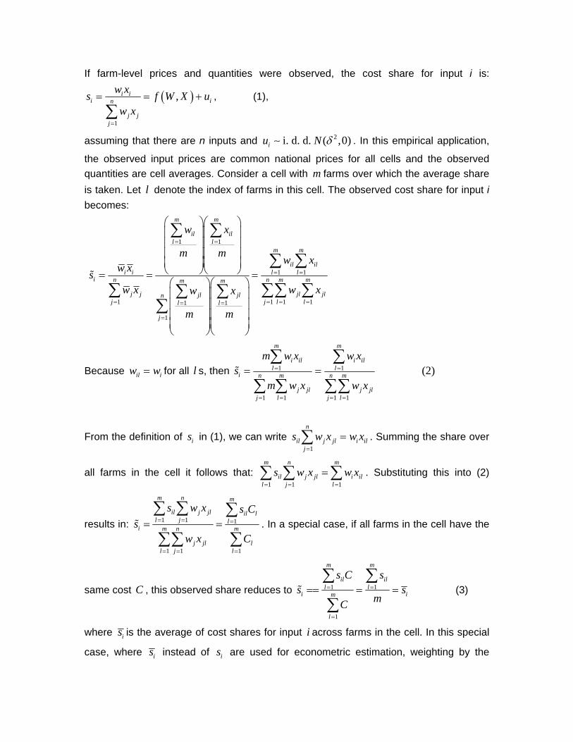
3.3. A unique feature of the Data – Adjusting for heteroskedasticity Perhaps the most important problem of this study is the potential heteroskedasticity in the econometric modelling due to the use of farm averages within each observational cell. Farms are normally assumed to act independently from each other and the error terms in econometric models using farm-level data are assumed to be identically and independently distributed (i.d.d.) with constant variance. The observed data used for econometric estimation in this study are average values and quantities across farms within the same production region, within the same industry and belonging to the same size category – an observational cell. This, together with the fact that sample size varies across the observational cells, implies that the variance of the error terms varies across observational units. (More accurately stated, the error terms’ variance decreases as the number of farms in the cell increases). This kind of heteroskedasticity is significantly more serious in this study than in preceding Australian studies (and international studies to the authors’ knowledge) where region, state or national average data are used. The robust econometric estimation requires some action to correct for heteroskedasticity or to alleviate its consequences. In a simple linear regression, the conventional means for overcoming this problem is to weight variables by the square root of the sample size (Wooldridge, 2006). While it is straightforward to arrive at the conclusion that such scaling is necessary for the quantity system derived from the normalized quadratic cost function, it is harder to determine whether it is also needed for the share system due to the appearance of the shares rather the quantities on the left-hand side of the corresponding equations. The following derivation leads to an answer that the share system also should be weighted during econometric estimation.

20

If farm-level prices and quantities were observed, the cost share for input i is:

( )

1

,i ii in

j jj

w xs f W Xw x

=

= =

∑u+ , (1),

assuming that there are n inputs and . In this empirical application,

the observed input prices are common national prices for all cells and the observed quantities are cell averages. Consider a cell with m farms over which the average share is taken. Let denote the index of farms in this cell. The observed cost share for input i becomes:

2i. d. d. ( ,0)iu N δ∼

l

1 1

1 1

1 11 1

1

m m

il ill l

m m

il ili i l l

i n nm m

1 1

m m

j j jjl jlnj jl l

j

w x

m m w xw xsw x w xw x

m m

= =

= =

= == =

=

⎛ ⎞⎛ ⎞⎜ ⎟⎜ ⎟⎜ ⎟⎜ ⎟⎜ ⎟⎜ ⎟⎜ ⎟⎜ ⎟⎝ ⎠⎝ ⎠= = =⎛ ⎞⎛ ⎞⎜ ⎟⎜ ⎟⎜ ⎟⎜ ⎟⎜ ⎟⎜ ⎟⎜ ⎟⎜ ⎟⎝ ⎠⎝ ⎠

∑ ∑

∑ ∑

∑ ∑∑ ∑∑

l jll l= =∑ ∑

Because for all s, then il iw w= l 1 1

1 1 1 1

m m

i il i ill l

i n m n m

j jl j jlj l j l

m w x w xs

m w x w x

= =

= = = =

= =∑ ∑

∑ ∑ ∑∑ (2)

From the definition of in (1), we can write . Summing the share over

all farms in the cell it follows that: . Substituting this into (2)

results in:

is1

n

il j jl i ilj

s w x w x=

=∑

1 1 1

m n m

il j jl i ill j l

s w x w x= = =

=∑ ∑ ∑

1 1 1

1 1 1

m n m

il j jl il ll j l

i m n m

j jl ll j l

s w x s Cs

w x C

= = =

= = =

= =∑ ∑ ∑

∑∑ ∑. In a special case, if all farms in the cell have the

same cost C , this observed share reduces to 1 1

1

m m

il ill l

i im

l

s C ss s

mC

= =

=

== =∑ ∑

∑= (3)

where is is the average of cost shares for input i across farms in the cell. In this special

case, where is instead of are used for econometric estimation, weighting by the is

21

square root of the sample size would be needed to account for heteroskedasticity. Despite the fact that the assumption that all farms within a cell have the same production cost may be unrealistic, the derivation above is to show that there would be some correlation between the cell sample size and the variance of the error terms, and that weighting is more likely to be appropriate than to ignore the effect. Moreover, the surveyed farms are classified into three farm sizes. Therefore, the total production cost for farms within a cell can be fairly similar to each other, which reinforces (3). Moreover, simple linear regressions actually show that, at least some linear relationships exist between the cell sample size and the squared estimated residuals obtained from the share system where no weighting is undertaken. So, weighting the share system is appropriate to correct heteroskedasticity caused by the nature of the quasi-micro data used in this study.

m

4. EMPIRICAL ESTIMATION AND RESULTS With five variable inputs, four outputs, eight exogenous variables and a time variable as described above, the system of cost share equations derived from the translog cost function is:

5 4 8

1 1 1ln ln lni i ij j il l ih h ti

j l hs w y z Tα α δ ρ γ

= = =

= + + + +∑ ∑ ∑ 1,2,...4i with = .

After adding an error term to each equation and leaving out the share equation of livestock trading input, the system consisting of share equations for Contracts, materials and services – livestock (CMS Livestock); Contracts, materials and services – cropping (CMS Cropping); Other contracts, materials and services (Other CMS); and Hired labour costs is estimated using the full information maximum likelihood (FIML) estimation method. The cost function is initially included in the equation system, but the estimation fails to give a result. Consequently the cost function is excluded from the system. (This exclusion is common in dual applications using the translog functional form). As discussed in Section 2.2, when the share system does not include the cost function itself, a cost share equation is dropped out of the system before the estimation proceeds. Using FIML, the parameter estimates are invariant to the equation being deleted from the system for the translog functional form. Parametric restrictions for symmetry and homogeneity conditions are imposed before the econometric estimation proceeds. With respect to the normalized quadratic cost function, any of the five variable costs can be chosen to be the normalizing factor or numeraire. Once the numeraire is decided, Shephard’s lemma is applied and a system consisting of four quantity demand equations

22

for the remaining inputs is derived. The homogeneity condition is maintained through the normalizing process and the symmetry condition is imposed parametrically during the FIML estimation. In this study, all systems with five alternative numeraires are estimated and the system with the best estimation results, judged on the basis of the proportion of significant own-price coefficients, the proportion of own-price coefficients that have correct (negative) signs and the percentage of significant coefficients in the whole system, is chosen. The invariance to the equation dropped out of the system does not hold for this functional form, implying that different normalizing factors result in different estimated relationships for the same input pairs. Once the share (quantity) system derived from the translog (normalized quadratic) cost function is estimated, the coefficient estimates and fitted shares (quantities) are used to calculate the Allen partial elasticities of substitution and price elasticities. The standard errors of the elasticities are estimated using the bootstrapping method following applications of Eakin, McMillen and Buono (1990), Green, Hahn and Rocke (1987), Krinsky and Robb (1986) and Freedman and Peters (1984). The bootstrapping method is used instead of the easier traditional first-order variance approximation (delta method) because the elasticities are nonlinear functions of the estimated coefficients. The bootstrapping procedure is described in detail in Appendix B.

4.1. Econometric estimation and coefficient estimates The estimated coefficients of the two equation systems derived from the two functional forms are presented in Table 3 and Table 4. For the estimation result of the translog cost share system, 73% (69 out of 95) of the system coefficients are significant at 5% significance level and all self-price coefficients ( iiα ) are highly significant. However, only

the own-price coefficients of the CMS Livestock and Hired labour equations have the expected signs. The percentages of negative share predictions (or violations of the monotonicity condition) are 4.1%, 14.7%, 0.3%, 21.7% and 13.2% for CMS Livestock; CMS Cropping; Other CMS; Hired labour; and Livestock trading inputs respectively. As shown in Table 4, the overall performance for the quantity system derived from the normalized quadratic cost function is not as good as that for the share system. The percentage of the significant coefficients is smaller (56%) and one self-price coefficient is not significant. The incidence of violating the monotonicity condition is also higher for this system compared to the estimated share system. All self-price coefficients iiα s,

however, are negative, even without imposition of this constraint. This implies that demand for an input decreases if its price increases, which is in accordance with economic theory.

23

In regards to nonprice variables, i.e. output quantities, dummy variables, rainfall and time trend, the coefficient estimates are generally statistically significant in both share and quantity systems. It is notable that beef output is highly significant in all equations of either system. Meanwhile, wool is not significant in all translog share equations, and similarly sheep is not significant in all but one share equations. These two outputs display greater statistical significance in the normalized quadratic quantity system. All other nonprice variables are significant in at least three out of five equations in the share system. They, except for the dummy variable Size 2, also have explanatory power in at least two out of four equations in the quantity system. Neither of the estimated systems satisfy the concavity condition. To check if the share

system meets the concavity condition, the matrix ˆ 'A s s s− + , where , is

the diagonal matrix with its diagonal elements being the fitted shares and is the column vector of the fitted shares, is computed and checked for negative semidefiniteness at each observational point (Diewert and Wales, 1987; and Terrell, 1996). This matrix is not negative semidefinite at almost all data points. For the quantity system derived from the normalized quadratic cost function, the estimated matrix

is not negative semidefinite. The attempt to estimate this system with the

negative semidefiniteness of

ij n nA α

×⎡ ⎤= ⎣ ⎦ s

n n× s

1ij n nα

− −×⎡ ⎤⎣ ⎦ 1

11ij n nα

− −×⎡ ⎤⎣ ⎦ being imposed using the Cholesky

factorization procedure as discussed in Section 2.3 fails to give a result. These results together indicate that the cost function is not concave in input prices.

Table 3: Estimated parameters for share system derived from translog cost function

Share equation CMS Livestock CMS Cropping Other CMS Hired labour Livestock trading Coefficients z-Stat. Coefficients z-Stat. Coefficients z-Stat. Coefficients z-Stat. Coefficients z-Stat. Intercept 0.766** 5.62 0.151 1.60 0.161 1.41 0.122** 3.23 -0.2** -3.65 CMS Livestock price -0.086** -6.88 0.023** 2.98 0.044** 4.51 0.008** 2.88 0.01** 3.01 CMS Cropping price 0.023** 2.98 0.108** 3.94 -0.234** -10.95 0.105** 4.69 -0.004 -1.14 Other CMS price 0.044** 4.51 -0.234** -10.95 0.222** 8.85 -0.013 -1.04 -0.019** -5.28 Hired labour price 0.008** 2.88 0.105** 4.69 -0.013 -1.04 -0.094** -3.38 -0.007** -4.24 Livestock trading price 0.01** 3.01 -0.004 -1.14 -0.019** -5.28 -0.007** -4.24 0.019** 8.75 Crops output quantity -0.003** -2.78 0.002** 2.90 0.001 0.72 0.000 -1.12 0.000 1.04 Sheep output quantity 0.001 0.30 0.002 1.07 0.003 1.57 0.000 -0.13 -0.005** -6.74 Beef output quantity 0.016** 6.91 -0.016** -14.66 -0.006** -3.36 0.003** 4.29 0.003** 3.47 Wool output quantity 0.000 -0.14 0.000 0.00 -0.001 -0.35 0.000 0.06 0.001 1.29 Capital -0.03** -4.61 0.004 0.92 -0.007 -1.22 0.018** 9.60 0.014** 5.21 Fixed labour -0.041** -3.81 -0.003 -0.36 0.064** 6.39 -0.032** -11.68 0.012** 2.59 Cropping industry -0.144** -18.84 0.114** 23.98 0.076** 12.76 -0.005** -2.69 -0.041** -13.00 Wheat Sheep zone 0.003 0.26 0.06** 6.99 -0.013* -1.65 -0.013** -5.43 -0.037** -14.49 High Rainfall zone -0.003 -0.26 0.083** 9.28 -0.03** -3.49 -0.017** -6.42 -0.033** -10.54 Size1: > $400,000 0.075** 6.27 0.056** 7.32 -0.123** -12.37 0.019** 5.84 -0.027** -5.53 Size2: $200,000-$400,000 0.043** 4.58 0.024** 4.27 -0.06** -8.36 0.009** 3.97 -0.015** -5.01 Annual rainfall 0.007 1.09 -0.004 -0.77 -0.014** -2.80 0.004** 2.12 0.008** 3.55 Time 0.003** 5.47 0.002** 3.85 -0.005** -9.90 0.001** 3.55 -0.002** -6.21

Note: ** Significant at 5% level

* Significant at 10% level

Table 4: Estimated parameters of quantity system derived from normalized quadratic cost function

Input quantity equation CMS-livestock CMS-Cropping Hired labour Livestock trading Coefficients z-Statistic Coefficients z-Statistic Coefficients z-Statistic Coefficients z-Statistic Intercept 78,674.9 0.88 -68,632.9** -3.30 527.8 0.06 -6,702.4 -0.99 CMS Livestock price -125,638.9** -3.30 788.0 0.15 -615.2 -0.27 4,821.9 1.51 CMS Cropping price 788.0 0.15 -22,975.7 -1.61 37,232.2** 3.51 1,115.0 0.74 Hired labour -615.2 -0.27 37,232.2** 3.51 -45,803.9** -3.23 -50.0 -0.08 Livestock trading price 4,821.9 1.51 1,115.0 0.74 -50.0 -0.08 -4,765.5** -5.37 Crops output quantity 0.017 0.28 0.13** 49.93 0.007** 3.83 -0.006** -2.00 Sheep output quantity 0.439** 3.11 0.122** 4.98 -0.007 -0.91 -0.029** -2.33 Beef output quantity 1.031** 55.39 -0.024** -3.71 0.056** 39.94 0.046** 33.58 Wool output quantity 0.154* 1.77 -0.03* -1.69 0.072** 15.69 -0.004 -0.58 Capital -0.112 -1.10 0.078** 4.55 0.075** 12.20 0.06** 9.85 Fixed labour -1.607** -3.14 -0.241** -3.16 -0.342** -11.93 0.156** 4.30 Cropping industry 3642.9 0.11 8,778.4** 2.85 4,397.9** 3.66 -2,615.5 -1.38 Wheat Sheep zone 164,010.7** 9.33 12,721.4** 3.19 -1,206.4 -1.07 -14,766.0** -9.42 High Rainfall zone 133,778.1** 4.96 13,701.1** 3.00 -2,774.3** -2.11 -13,004.8** -8.57 Size1: > $400,000 25,642.4 0.74 31,415.7** 6.98 6,393.9** 3.60 2,211.1 0.97 size2: $200,000-$400,000 21,095.7 0.66 7,373.6* 1.74 -182.6 -0.11 -526.0 -0.26 Annual rainfall -15,653.2 -1.16 5,942.2** 2.74 961.9 0.99 3270.3** 3.37 Time 127.2 0.07 1,641.6** 6.41 886.5** 4.69 -401.4** -3.18

Note: ** Significant at 5% level

* Significant at 10% level

4.2. Estimated elasticities ( ijσ and ijη )

Estimated Allen partial elasticities of substitution (with their bootstrapping standard errors) from the two functional forms are shown in Table 5 and Table 6. The two results give the same substitution and complementarity relationships for pairs of inputs except for the CMS Livestock – Hired labour pair. Almost all inputs are substitutes to each other, except for the CMS Cropping – Other CMS and Livestock trading – Hired labour pairs. With an exception of the relation between CMS Cropping and Hired labour, the degrees of substitution and complementarity are generally small. The computed elasticity of substitution between CMS Cropping and Hired labour is very large, 13.6 for the translog cost function and 15.6 for the normalized quadratic function. For the CMS Livestock – Hired labour pair, the translog cost function indicates that they are substitutes while the normalized quadratic function states the opposite. Table 5: Allen partial elasticities of substitution - Translog functional form a, b

Contracts, materials & services _ Livestock

Contracts, materials & services _ Cropping

Other contracts, materials & services

Hired labour

Livestock trading

Contracts, materials & services _ Livestock . Contracts, materials & services _ Cropping 1.83 . (0.193) Other contracts, materials & services 1.37 -1.38 . (0.068) (0.211) Hired labour 1.77 13.60 0.46 . (0.22) (2.311) (0.445) Livestock trading 1.83 0.40 0.24 -1.79 . (0.147) (0.235) (0.089) (0.356) Note: a Medians of elasticities evaluated at all observation points b Bootstrapping Standard Errors (1000 trials) are in parentheses

27

Table 6: Allen partial elasticities of substitution - Normalized quadratic functional form a, b

Contracts, materials & services _ Livestock

Contracts, materials & services _ Cropping

Other contracts, materials & services

Hired labour

Livestock trading

Contracts, materials & services _ Livestock . Contracts, materials & services _ Cropping 0.052 . (0.002) Other contracts, materials & services 1.651 -0.603 . (0.036) (0.016) Hired labour -0.100 15.571 0.573 . (0.003) (0.479) (0.023) Livestock trading 1.385 0.818 0.493 -0.072 . (0.042) (0.024) (0.021) (0.003) Note: a Medians of elasticities evaluated at all observation points b Bootstrapping Standard Errors (200 trials) are in parentheses

Table 7 and Table 8 respectively present own- and cross-price elasticities (and their bootstrapping standard errors) estimated from the translog and normalized quadratic systems. Both results have negative own-price elasticities, which is as expected. Most corresponding elasticities in the two tables have the same signs, indicating that the two functional forms give the same directions in their estimated responsiveness of input demands to price changes. As shown in the two tables, demands for most inputs are inelastic with respect to their own prices and prices of other alternative inputs. Notably, demand for Hired labour is highly responsive, but in opposite directions, to its own price and CMS Cropping price with magnitudes being greater than two in either functional form. This implies that a 1-percent change in these two prices will lead to a greater than 2-percent change in demand for Hired labour. The elasticity of demand for CMS Cropping with respect to Hired labour also ranks high in absolute value compared to other elasticity estimates. In addition, two sets of elasticities show that around three quarters of the calculated elasticities are statistically significant. An obvious difference between the two results is that the own-price elasticity of demand for CMS Livestock estimated from the translog function is -1.139 compared to -0.868 from the normalized quadratic function.

28

Table 7: Own- and cross-price elasticities - Translog functional form a, b

Price

Quantity

Contracts, materials & services - Livestock

Contracts, materials & services - Cropping

Other contracts, materials & services

Hired labour

Livestock trading

Contracts, materials & services _ Livestock -1.139 0.217 0.745 0.075 0.098 (0.041) (0.025) (0.033) (0.012) (0.015) Contracts, materials & services _ Cropping 0.313 -0.215 -0.728 0.620 0.007 (0.031) (0.137) (0.111) (0.109) (0.021) Other contracts, materials & services 0.298 -0.312 -0.036 -0.001 -0.004 (0.018) (0.041) (0.048) (0.022) (0.007) Hired labour 0.409 2.357 0.237 -2.901 -0.098 (0.061) (0.43) (0.232) (0.501) (0.026) Livestock trading 0.480 0.020 0.118 -0.115 -0.546 (0.049) (0.052) (0.047) (0.016) (0.022) Note: a Medians of elasticities evaluated at all observation points b Bootstrapping Standard Errors (1000 trials) are in parentheses

Table 8: Own- and cross-price elasticities - Normalized quadratic functional form Price

Quantity

Contracts, materials & services _ Livestock

Contracts, materials & services _ Cropping

Other contracts, materials & services

Hired labour

Livestock trading

Contracts, materials & services _ Livestock -0.868 0.009 0.790 -0.006 0.063 (0.065) (0.018) (0.067) (0.01) (0.041) Contracts, materials & services _ Cropping 0.013 -0.638 -0.364 0.935 0.042 (0.197) (0.197) (0.127) (0.021) (0.059) Other contracts, materials & services 0.363 -0.117 -0.334 0.045 0.030 (0.076) (0.123) (0.034) (0.012) (0.037) Hired labour -0.021 2.006 0.280 -2.300 -0.003 (0.334) (0.235) (0.414) (0.024) (0.054) Livestock trading 0.407 0.152 0.259 -0.006 -0.887 (0.056) (0.06) (0.022) (0.031) (0.077) Note: a Medians of elasticities evaluated at all observation points b Bootstrapping Standard Errors (200 trials) are in parentheses

4.3. Technology Tests

It is possible using the cost function to examine whether the underlying production technological structure has certain characteristics such as diminishing/constant/increasing returns to scale or nonjointness and separability of inputs and outputs. In this study, since the cost function is excluded from the share/quantity system, it is not possible to conduct tests for increasing or decreasing returns to scale because lkβ s are not estimated. It is, however, possible to test for input

separability. Subject to homogeneity and symmetry, the parametric restriction test for

29

separability of all inputs using the normalized quadratic functional form is: 0 ,ij i jα = ∀ ≠ and . This joint equality test is rejected at 5%

significance level using the Wald statistic. Inspection of the system estimates reveals that the equations of CMS Livestock and Livestock trading quantities have insignificant coefficients for all other alternative input prices. The joint test for these coefficients being equal to zero has a p-value of 0.70, suggesting that demands for CMS Livestock and Livestock trading are independent of other input prices.

, 1,2,i j n= … 1−

4.4. Discussion of results The econometric estimation results are overall robust for the cost function using translog and normalized quadratic functional forms. The implied elasticities of substitution and price elasticities from the two systems are in line with each other in terms of the direction of the pair-wise relationships. A majority of these measures are also statistically significant and all own-price elasticities have the expected signs. The two sets of the Allen partial elasticities of substitution are generally small and comparable to those in McKay, Lawrence and Vlastuin (1982)’s study of Wheat/sheep zone. (The comparison may not be accurate due to differences in geographical coverage, nature of data used, functional forms used, and data aggregation in econometric estimation but provides some basis for validating the results found in this study). The high degree of substitution between Hired labour and CMS Cropping can be explained by the fact that many production tasks involved in cropping are not as highly skilled as those involved in livestock production (possibly with the help of mechanization in production process) that can be substituted for by low skilled hired labour. Due to differences in geographical coverage, the nature of data used, data aggregation methods, the objective function estimated and the functional form used, it is not possible to compare the estimated parameterized input equations and the implied elasticities of substitution and price elasticities in this study to those in previous studies. However, in their estimation of profit functions for Western Australian broadacre production, Coelli (1996) and Ahammad and Islam (2004) found that demand for labour (mixture of hired labour and other labour sources) is more responsive to its own price and crop prices than to the prices of animal products. This finding, to some extent, shares the same trend as the results in this study that demand for Hired labour is more elastic to its own price and CMS Cropping price than to CMS Livestock, Other CMS and Livestock trading prices. Besides, the high demand-price responsiveness between Hired labour and CMS Cropping is in agreement with findings on their substitutability measured by the Allen partial elasticities. However, it is noteworthy that due to the use of national input price indices in the estimation, the resulting price elasticities may be higher than what they

30

should be, especially for the case of Hired labour demand with respect to its own price and CMS Cropping price. The data on input quantities are at a quasi-micro farm level while price data are at a national level. This mismatch in data implies that for a given price change the demand response is greater than it would be if quantities at a state, region or national level were used. This will result in higher price elasticities. This effect, however, may be offset by the reduction in the effects that data aggregation has on parametric and elasticity estimates. As in many previous studies, the two systems of shares and quantities derived from the two functional forms in this study do not satisfy parametric restrictions for the concavity condition. The imposition of this condition using Cholesky factorization in the normalized quadratic system also did not succeed. This can also be partly explained by the nature of the data used for the estimation. In this study, for a given year, input prices are the same across observational points but, because of the nature of quasi-micro data, input quantities vary greatly. This, in effect, reduces or straightens any curvature present in the cost function. Moreover, for the same year-to-year change, the directions in demand response are not necessarily the same from an observational cell to another. The price changes individual farms face are not the same and are not exactly what is reflected in the movements in the national price index numbers. These two insights can help explain the failure of the cost function in meeting the concavity condition in this study. 5. CONCLUSION Technological and economic relationships between production inputs in the Australian broadacre sector have been estimated in this paper, using a multi-product restricted cost function framework and a unique quasi-micro farm-level data drawn from the AAGIS. Issues and problems distinctive to this study, especially heteroskedasticity due to the quasi-micro nature of the data, are accommodated. Estimation results from the translog and normalized quadratic functional forms are robust with high proportions of significant parameters. The Allen partial elasticities of substitution, and own- and cross-price elasticities derived from both functional forms have the expected signs. The two functional forms are in agreement with each other in terms of the direction of relationships between input pairs. The estimated empirical results and measures in this study are at a national level as all broadacre production regions are included in the data. They are useful for social and economic assessment, and policy developments for the Australian rural sector as a whole. It is found that most production inputs are substitute to each other. The aggregate Contracts, materials and services for cropping input is highly substitutable for Hired labour and vice versa. Most production inputs are also found to be unresponsive to changes in own prices or other input prices. Demand for Hired labour is highly

31

responsive to own price and price of Contracts, materials and services for cropping. Moreover, structural tests using the normalized quadratic functional form indicate that demands for Contracts, materials and services for livestock and for Livestock trading are separable from other input demands. This implies that there is some degree of independence between livestock and cropping production in the short run. Symmetry and homogeneity conditions were imposed during the econometric estimation while monotonicity and concavity conditions were checked afterwards. The monotonicity condition is violated at a significant percentage of data points, and the concavity condition is not satisfied by the estimated cost function, using either functional form. This may be attributable to the quasi-micro nature of the data used and the unavailability of input prices actually paid by individual observational units. The observed input quantities are at a quasi-micro level while the observed prices are at a national level. It should also be noted that this mismatch in the data may have inflated the price responses.

32

APPENDIX A: DATA AGGREGATION

A.1. Inputs Contracts, Services and Materials for Livestock Production factors that are aggregated into the Contracts, services and materials for livestock (CSM Livestock) index are fodder, livestock materials, livestock purchases, contracts for livestock, AI stud herd test, vet fees, agistment expense, stores and rations, and shearing and crutching. The corresponding price indices for these production inputs sourced from ABARE’s Australian Commodities Statistics – Producer Paid Prices are those under the labels: fodder and feedstuffs, chemicals and medicines, contracts, and shearing rates. The quantities of these inputs are derived by dividing the individual expenses on these inputs by their corresponding ABARE producer paid price index numbers. The resulted quantities and the ABARE price indices are then used to construct the aggregate CSM Livestock quantity and price indices. In this construction, there is a need to fully account for the livestock that are actually brought into production during each surveyed year. This is done by adding negative operating gains and livestock transferred onto the farm during the surveyed year to the recorded livestock purchases. While the quantity and value of livestock purchases both are observed, only the values of the operating gains and inward transfers are available. Therefore, the quantities of these two movements are calculated as their values are divided by the corresponding selling prices. Contracts, Services and Materials for Cropping For the aggregate price and quantity indices of the Contracts, services and materials for cropping (CSM Cropping), the component inputs are seed, fertilizer, crop – pasture chemicals, and contracts for cropping. The aggregation process is similar to that followed in the aggregation of CSM Livestock. The ABARE Australian Commodities Statistics – Producer Paid Prices indices for seed, seedlings and plants, fertilizer, chemicals and medicines, and contracts are again used in place of the actual paid prices. Other Contracts, Services and Materials The Other contracts, services and materials (Other CSM) aggregate indices are constructed based on the rest of production inputs except for the hired labour which stands on its own in the estimation model. They are fuel, oil and grease, electricity, repairs buildings structure, repairs machinery and plant, handling and marketing, total

33

freight, interest paid, rates, insurance, land rent, lease, telephone, other administrative items, rates and drain water, accountancy fee, advisory services, other materials and other services. Respectively, the ABARE producer paid price indices used are Fuel and Lubricants, Electricity, Maintenance – Structure, Maintenance – Plant and Equipment, Selling expenses, Freight outwards, Interest paid, Rates and Taxes, Insurance, Other overheads, and Other materials and services. Hired Labour Hired labour quantity and price indices are constructed based on the total expense on hired labour and the index for wages available from the ABARE Australian Commodities Statistics – Producer Price Paid and thus the quantity index can be derived implicitly. Livestock Trading The last item in the catalogue of the variable inputs is the Livestock trading. Livestock can be thought as a capital item due to the fact that only part of the total stock of livestock at the beginning of each production period will be consumed during that period. For instance, only those cattle or sheep that reach their final stage of the production process will be turned off while others are carried over to the next production cycle. The farmers, however, can adjust the levels of livestock on hold within a fairly short time period if she/he view such action is profitable or necessary for survival. This renders the livestock holdings having the nature of the variable production factors. One way to account for these two facets in the nature of livestock held is to estimate the service cost of livestock and treat it as a variable input in the estimation model. It is referred to as Livestock trading in this study. The service cost is formulated as being equal to the opening balance of livestock on hold multiplied by the real interest rate. The quantity of the service cost for livestock is assumed to be proportional to the livestock level. The data on the opening balance of livestock on hold is not available. It is, therefore, derived using other available information. In this study, the derivation of this figure is based on the estimation of the number of livestock held at the beginning of year and the average of livestock purchasing and selling prices. The opening number of livestock is equal to the number of livestock at the end of the year plus the number of livestock turned off minus the number of livestock purchased or transferred in and minus the estimated number of livestock operating gains. The estimated opening number of livestock is then multiplied by the average livestock purchasing and selling prices to arrive at the opening value of livestock on hold. The real interest rate is calculated as the nominal interest rate of three-year fixed term deposits in retail banking minus the inflation rate. The monthly interest rates for this

34

category of term deposits are available from the RBA website and are averaged to give rise to the yearly rate. The two-year moving average of this yearly interest rate series is used to calculate the service cost.

A.2. Capital Total capital The physical capital used in farm production are incorporated as fixed inputs in the estimation model. This is justified by the fact that it usually takes more than one production cycle for farmers to adjust the amounts of land, building and other fixed improvements as well as plants and machinery to respond to market changes. The figures needed for the estimation model is the opening balances of these capital items. However, the opening balance of the capital stocks are not included in the ABARE’s dataset received and have to be calculated using other available information. The following formula: Opening balance = Closing balance + Depreciation - Net capital additions - Total imputed capital appreciation, is used in this study for this purpose. Ideally, the capital items should be treated separately as individual items because of the differences in how they are utilized in farming and the rate at which they depreciate. Since there no data on depreciation of individual capital items, one aggregate capital variable which is the sum of land, buildings and other fixed improvements, and plants and machineries is created. Due to missing data in closing balance of plants and machineries, an alternative calculation is proposed where Opening balance of total capital = Farm equity closing balance/Equity ratio*100 + Depreciation - Net capital additions - Total imputed capital appreciation - Calculated opening livestock capital. With this calculated opening balance, the service cost of the capital is estimated as the opening balance multiplied by the real interest rate plus the depreciation costs. The resulting service cost of capital, together with the price index of capital published in the annual ABARE Australian Commodities Statistics, are then used to create the implicit index of capital quantity. Fixed labour For quantity and price indices of the operator’s and family’s labour, the quantity is the total worked weeks adjusted for the estimated number of weeks worked by hired labour. Assuming that hired labour and fixed labour receive the same wage, the number of weeks worked by the operator and his/her family are the ratio of the total hired labour cost over the imputed labour cost multiplied by the total number of weeks worked by all labours. The value of this fixed input is the imputed labour cost variable recorded by ABARE in the requested dataset. The price index is derived implicitly by dividing the imputed labour cost by the quantity index.

35

A.3. Outputs

The construction of quantity and price indices for outputs is less complicated than that of the variable and fixed inputs since both value and quantity of individual outputs are observed in the dataset. With the available data on value and quantity, the actual price received by each observational unit (a group of farms in the same production region, same industry and same size category) for each output is derived by dividing the corresponding value by the corresponding quantity. With these three price, quantity and value variables, the construction of aggregate price and quantity indices is straightforward. Wheat and Other crops Wheat is grouped with barley, oats, grain legumes, oilseeds, canola, field peas, lupins and sorghum under the Wheat and Other grain category. Their values are observed as gross receipts in the dataset used. Sheep Sheep and Wool outputs are incorporated into the estimation model separately. The quantity of sheep is the number of sheep sold, adjusted by the positive sheep inventory gain, and the sheep selling price equals the sum of gross receipt for sheep and divided by the number of sheep sold. The value of sheep sold plus the value of positive sheep inventory gain is the total value of sheep produced. For Wool, total value of wool production is equal to the actual wool price received, which is calculated as the gross receipt for wool divided by kilograms of wool sold, multiplied by number of kilograms of wool actually produced. Wool Beef and Other livestock Beef is grouped with Other livestock sold. There is a need for adjustments in the quantity of beef sold due to changes in beef inventory during the surveyed year. The number of beef turnoff, which is the sum of the number of beef sold and number of beef transferred out, is used instead of number of beef sold. The positive beef inventory (operating) gain is added to the value of beef produced (or turned off). The number of beef operating gain is approximated by dividing the value of beef operating gain by the average of beef purchasing and selling prices. The beef selling price equal gross receipts from beef divided by quantity of beef sold. The index of price received for the overall livestock

36

sector from the annual ABARE Australian Commodities Statistics is used for the price index of the Other livestock component. APPENDIX B: ESTIMATING STANDARD ERRORS USING BOOSTRAPPING Applications of the bootstrapping method to calculate the standard errors of elasticities include Eakin et al. (1990), Green et al. (1987), Krinsky and Robb (1986) and Freedman and Peters (1984). This study follows the procedure of calculating the standard errors described in Eakin et al. (1990), which is as follows:

1. Run the estimation of share/quantity systems using FIML. 2. Create and save the residuals from the system. 3. Create a new sample of residuals by drawing randomly with replacement from

the estimated residuals (bootstrapping). 4. Create an artificial sample of the dependent variables by adding the newly

drawn sample of residuals to the fitted values of dependent variables from Step 1.

5. Run the estimation of share/quantity systems using FIML using the artificial sample of the dependent variables and the actual sample of the independent variables.

6. Calculate and save Allen partial, own-price and cross-price elasticities using the estimated parameters and predicted shares/quantities from Step 5.

7. Save the median of the calculated elasticities 8. Repeat the procedure described in Step 3 to step 7 (a trial) for a number of

times – (1000 trials for the share system and 200 trials for the quantity system) 9. Standard errors of the distribution of the medians of the elasticities repeatedly

calculated from all the trials are the standard errors of interest.

37

REFERENCES: Ahammad H, Islam N (2004) Regional agricultural production systems: estimates for Western Australia. Review of Urban and Regional Development Studies 16, 189-209. Anderson DP, Chaisantikulawat T, Guan ATK, Kebbeh M, Lin N, Shumway CR (1996) Choice of Functional Form for Agricultural Production Analysis. Review of Agricultural Economics 18, 223-231. Barnett WA, Hahm JH (1994) Financial-Firm Production of Monetary Services: A Generalized Symmetric Barnett Variable-Profit-Function Approach. Journal of Business and Economic Statistics 12, 33-46. Berndt ER, Khaled MS (1979) Parametric Productivity Measurement and Choice among Flexible Functional Forms. Journal of Political Economy 87, 1220-1245. Binswanger HP (1974a) A Cost Function Approach to the Measurement of Elasticities of Factor Demand and Elasticities of Substitution. American Journal of Agricultural Economics 56, 377-386. Blackorby C, Primont D, Russell RR (1977) On testing separability restrictions with flexible functional forms. Journal of Econometrics 5, 195-209. Caves DW, Christensen LR (1980) Global Properties of Flexible Functional Forms. The American Economic Review 70, 422-432. Chalfant JA (1984) Comparison of Alternative Functional Forms with Application to Agricultural Input Data. American Journal of Agricultural Economics 66, 216. Chambers RG (1988) 'Applied production analysis : a dual approach ' (Cambridge [England] New York : Cambridge University Press). Christensen LR, Jorgenson DW, Lau LJ (1973) Transcendental Logarithmic Production Frontiers. The Review of Economics and Statistics 55, 28-45. Coelli TJ (1996) Measurement of total factor productivity growth and biases in technological change in Western Australian Agriculture. Journal of Applied Econometrics 11, 77-91. Diewert WE (1971) An Application of the Shephard Duality Theorem: A Generalized Leontief Production Function. Journal of Political Economy 79, 481-507. Diewert WE, Wales TJ (1987) Flexible functional forms and global curvature conditions. Econometrica 55, 43-68. Eakin BK, McMillen DP, Buono MJ (1990) Constructing Confidence Intervals Using The Bootstrap: An Application To A Multi-Product Cost Function. Review of Economics and Statistics 72, 339-344.

38

Fisher BS, Wall CA (1990) Supply response in the Australian sheep industry: a profit function approach. Australian Journal of Agricultural and Resource Economics 34, 147-166. Fisher D, Fleissig A, Serletis A (2001) An empirical comparison of flexible demand system functional forms. Journal of Applied Econometrics 16, 59-80. Freedman DA, Peters SC (1984) Bootstrapping a Regression Equation: Some Empirical Results. Journal of the American Statistical Association 79, 97-106. Gagne R, Ouellette P (1998) On the choice of functional forms: Summary of a Monte Carlo experiment. Journal of Business and Economic Statistics 16, 118-124. Gallant AR (1984) The Fourier Flexible Form. American Journal of Agricultural Economics 66, 204-208. Green R, Hahn W, Rocke D (1987) Standard errors for elasticities: A comparison of bootstrap and asymptotic standard errors. Business and Economic Statistics 5, 145-149. Halvorsen R, Smith TR (1986) Substitution Possibilities for Unpriced Natural Resources: Restricted Cost Functions for the Canadian Metal Mining Industry. The Review of Economics and Statistics 68, 398-405. Hotelling H (1932) Edgeworth's taxation paradox and the nature of demand and supply functions. Journal of Political Economy 40, 577-616. Ivaldi M, Ladoux N, Ossard H, Simioni M (1996) Comparing Fourier and translog specifications of multiproduct technology: Evidence from an incomplete panel of French farmers. Journal of Applied Econometrics 11, 649-667. Kohli U (1994) Canadian Imports and Exports by Origin and Destination: A Semi-Flexible Approach. The Canadian Journal of Economics / Revue canadienne d'Economique 27, 580-603. Krinsky I, Robb AL (1986) On Approximating The Statistical Properties Of Elasticities. Review of Economics and Statistics 68, 715-719. Lau LJ (1974) Applications of duality theory: a comment. In 'Frontiers of quantitative economics'. (Eds MD Intriligator, DA Kandrick) pp. 176-199Amserdam: North-Holland). Lawrence D (1989) An Aggregator Model of Canadian Export Supply and Import Demand Responsiveness. The Canadian Journal of Economics / Revue canadienne d'Economique 22, 503-521. Lim H, Shumway CR (1997) Technical Change and Model Specification: U.S. Agricultural Production. American Journal of Agricultural Economics 79, 543-554. Liu Q, Shumway CR (2004 ) Testing aggregation consistency across geography and commodities. 48, 463-486.

39

Lopez RE (1984) Estimating Substitution and Expansion Effects Using a Profit Function Framework. American Journal of Agricultural Economics 66, 358-367. McFadden D (1978) Cost, revenue and profit functions. In 'Production Economics: A Dual Approach to Theory and Applications'. (Eds M Fuss, D McFadden). (3–109: North-Holland, Amsterdam). McKay L, Lawrence D, Vlastuin C (1982) Production Flexibility and technical change in Australia's Wheat-Sheep zone. Review of Marketing and Agricultural Economics 50, 9-26. McKay L, Lawrence D, Vlastuin C (1983) Profit, Output Supply, And Input Demand Functions For Multiproduct Firms: The Case Of Australian Agriculture. International Economic Review 24, 323-339. Morrison Paul CJ (2001) Market and Cost Structure in the U.S. Beef Packing Industry: A Plant-Level Analysis. American Journal of Agricultural Economics 83, 64-76. Moschini G (1988) A Model of Production with Supply Management for the Canadian Agricultural Sector. American Journal of Agricultural Economics 70, 318-329. Mullen JD, Cox TL (1996) Measuring productivity growth in Australian broadacre agriculture. Australian Journal of Agricultural Economics 40, 189-210. Ollinger M, MacDonald JM, Madison M (2005) Technological Change and Economies of Scale in U.S. Poultry Processing. American Journal of Agricultural Economics 87, 116-129. Polson R, Shumway CR (1990) Structure of South Central Agricultural Production. Southern Journal of Agricultural Economics, 153-163. Rask K (1995) The Structure of Technology in Brazilian Sugarcane Production, 1975-87: An Application of a Modified Symmetric Generalized McFadden Cost Function. Journal of Applied Econometrics 10, 221-232. Shephard RW (1953) 'Cost and production functions.' (Princeton University Press: Princeton). Shumway CR (1983) Supply Demand, and Technology in a Multiproduct Industry: Texas Field Crops. American Journal of Agricultural Economics 65, 748-760. Shumway CR, Davis GC (2001) Does consistent aggregation really matter? The Australian Journal of Agricultural and Resource Economics 45, 161-194. Terrell D (1996) Incorporating Monotonicity and Concavity Conditions in Flexible Functional Forms. Journal of Applied Econometrics 11, 179-194. Thompson GD, Langworthy M (1989) Profit Function Approximations and Duality Applications to Agriculture. American Journal of Agricultural Economics 71, 791-798

40

Villezca-Becerra P, Shumway CR (1992) Multiple-output production modeled with three functional forms. Journal of Agricultural and Resource Economics 17, 13-28. Wooldridge JM (2006) 'Introductory econometrics: A modern approach.' (Thomson South-Western). Yotopoulos PA, Lau LJ, Wuu-Long L (1976) Microeconomic Output Supply and Factor Demand Functions in the Agriculture of the Province of Taiwan. American Journal of Agricultural Economics 58, 333-340