Climate-adjusted productivity for broadacre cropping farms
71
Farm performance and climate Climate-adjusted productivity for broadacre cropping farms Research by the Australian Bureau of Agricultural and Resource Economics and Sciences May 2017 Research Report 17.4 Department of Agriculture and Water Resources Neal Hughes, Kenton Lawson, Haydn Valle
Transcript of Climate-adjusted productivity for broadacre cropping farms
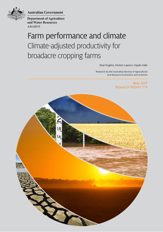
Farm performance and climate Climate-adjusted productivity for broadacre cropping farms
Research by the Australian Bureau of Agricultural and Resource Economics and Sciences
May 2017 Research Report 17.4
Department of Agricultureand Water Resources
Neal Hughes, Kenton Lawson, Haydn Valle

© Commonwealth of Australia 2017
Ownership of intellectual property rights
Unless otherwise noted, copyright (and any other intellectual property rights, if any) in this publication is owned by the Commonwealth of Australia (referred to as the Commonwealth).
Creative Commons licence
All material in this publication is licensed under a Creative Commons Attribution 3.0 Australia Licence, save for content supplied by third parties, logos and the Commonwealth Coat of Arms.
Creative Commons Attribution 3.0 Australia Licence is a standard form licence agreement that allows you to copy, distribute, transmit and adapt this publication provided you attribute the work. A summary of the licence terms is available from creativecommons.org/licenses/by/3.0/au/deed.en. The full licence terms are available from creativecommons.org/licenses/by/3.0/au/legalcode.
Cataloguing data
Hughes, N, Lawson, K & Valle, H 2017, Farm performance and climate: Climate-adjusted productivity for broadacre cropping farms, Canberra, April. CC BY 3.0.
ISSN 1447-8358 ISBN 978-1-74323-337-5 ABARES research report 17.4
Internet Farm performance and climate: Climate-adjusted productivity for broadacre cropping farms is available at agriculture.gov.au/abares/publications.
Contact
Australian Bureau of Agricultural and Resource Economics and Sciences (ABARES)
Postal address: GPO Box 858 Canberra ACT 2601 Switchboard: +61 2 6272 3933 Email: [email protected] Web: agriculture.gov.au/abares
Inquiries about the licence and any use of this document should be sent to [email protected].
The Australian Government acting through the Department of Agriculture and Water Resources, represented by the Australian Bureau of Agricultural and Resource Economics and Sciences, has exercised due care and skill in preparing and compiling the information and data in this publication. Notwithstanding, the Department of Agriculture and Water Resources, ABARES, its employees and advisers disclaim all liability, including for negligence and for any loss, damage, injury, expense or cost incurred by any person as a result of accessing, using or relying on information or data in this publication to the maximum extent permitted by law.
This project has benefited from discussions with ABARES staff including Alistair Davidson, Mathew Miller, Tom Jackson and Peter Gooday. Comments on drafts of this report were received from Terence Farrel at the Grains Research and Development Corporation (GRDC), Zvi Hochman at the CSIRO and Tiho Ancev at the University of Sydney.

iiiABARESFarm performance and climate
Contents
Summary 1
Motivation 1
Key findings 2
Future research 4
1 Introduction 5
Background 5
This study 6
2 Previous research 7
Productivity and climate 7
Recent climate trends 8
Crop yields and recent climate trends 9
Long-term climate change projections 9
3 Data 11
Farm data 11
Climate data 14
Additional data 17
4 Methods 18
Effect of climate on productivity 18
A data–driven approach 18
5 Results 20
Total factor productivity 20
Wheat yields 33
6 Future research 38
Monitoring productivity change 38
Informing risk management systems 38
Analysing larger data sets 39
From productivity to profit 39

iv ABARESFarm performance and climate
Contents
Appendix A: Machine learning methods 40
Gradient-boosted regression trees 40
Cross-validation 40
Feature selection 42Meta-parameters 42
Model testing 42
Average response curves 44
Appendix B: Calculating climate-adjusted productivity 51
Climate adjusted productivity 51
Climate effects 52
Calculating averages 52
Decomposing climate-adjusted productivity 52
Appendix C: Changes in Australian cropping areas 54
References 62
Tables
1 Average annual growth in climate-adjusted productivity for selected periods, regions and industries (%) 22
2 Average annual climate effect on total factor productivity levels for selected periods, regions and industries (%) 25
3 Effect of dry conditions on TFP relative to long-run average conditions for selected years, regions and industries (%) 26
4 Effect of wet conditions on TFP relative to long-run average conditions for selected years, regions and industries (%) 27
5 Average annual growth in wheat yields for selected periods, regions and industries (%) 34
6 Average annual climate effect on wheat yields, , for selected periods, regions and industries (%) 35
7 Effect of dry conditions on wheat yield relative to long-run average conditions for selected years, regions and industries 36
8 Effect of wet conditions on wheat yield relative to long-run average conditions for selected years, regions and industries 36
9 Final meta-parameter values 42
10 Cross–validated of the TFP model for selected regions, industries and time periods 44
Figures
1 Average climate-adjusted productivity for cropping specialist farms, 1977–78 to 2014–15 2
2 Map of average climate effect on productivity levels since 2000–01, (relative to the 1914–15 to 2014–15 average conditions) 3
3 Average winter season rainfall in Australia since 1996 8
4 Projected effect of climate change on the TFP of wheat growing farms by 2030 10
5 Average sample density of cropping farms, 1977–78 to 2014–15 11
6 Annual sample means for selected farm variables, 1977–78 to 2014–15 13
7 Climate data the bias—variance trade–off 14
8 Climate variable time periods relative to survey (financial) year 15
9 Annual sample means for selected climate variables, 1977–78 to 2014–15 16
10 Average climate-adjusted productivity for all cropping farms, 1977–78 to 2014–15 20
11 Average climate-adjusted productivity for cropping specialists, 1977–78 to 2014–15 21

vABARESFarm performance and climate
Contents
12 Australian grain farm terms of trade, 1977–78 to 2014–15 22
13 Average land prices and capital investment on cropping farms, 1977–78 to 2014–15 23
14 Average climate effect on productivity levels since 2000–01, relative to the 1914–15 to 2014–15 average 24
15 Total factor productivity under dry and wet conditions ( , ), 1977–78 to 2014–15 25
16 Effect of dry and wet years on TFP, 1977–78 to 2014–15 26
17 Adoption of no–till cropping practices by state 28
18 Decomposition of climate adjusted total factor productivity, 1977–78 to 2014–15 29
19 Effect of time (technology) on total factor productivity by region, 1977–78 to 2014–15 29
20 Other (scale) effects on total factor productivity by region, 1977–78 to 2014–15 29
21 Change in sample density of cropping farms between 2001–2015 relative to 1990–2000 30
22 Percentage change in cropping area by Statistical Local Area (SLA) between 2000–01 and 2010–11 31
23 Farm location effect on total factor productivity by region, 1977–78 to 2014–15 32
24 Average climate-adjusted wheat yields, 1977–78 to 2014–15 32
25 Average climate effect on wheat yield levels since 2000–01, relative to 1914–15 to 2014–15 34
26 Effect of dry and wet years on wheat yields, 1977–78 to 2014–15 35
27 Decomposition of climate adjusted wheat yield, 1977–78 to 2014–15 37
28 Climate variable importance rankings TFP model 41
29 Climate variable importance rankings W_YIELD model 41
30 Model estimation process 42
31 Model performance (cross-validated ) 43
32 National average annual total factor productivity predicitions (in–sample), 1977–78 to 2014–15 43
33 Average response of climate-adjusted TFP to AREA 45
34 Average response of climate-adjusted TFP to LIVESTOCK 45
35 Average response of climate-adjusted TFP to AGE 45
36 Average response of climate-adjusted TFP to FLOOD20 46
37 Average response of climate-adjusted W_YIELD to W_AREA 46
38 Average response of predicted W_YIELD to FLOOD1_5 47
39 Average response of predicted TFP to WINTER_RAIN 47
40 Average response of predicted TFP to TWO_YEAR_LAG_RAIN 48
41 Average response of predicted TFP to SPR_RAIN 48
42 Average response of predicted W_YIELD to WINTER_RAIN 49
43 Average response of predicted W_YIELD to SUMMER_LAG_RAIN 49
44 Average response of predicted W_YIELD to WIN_TMAX 50
45 Average response of predicted W_YIELD to SPR_TMIN 50
46 Total Australian cropping area and total agricultural area, 1992–93 to 2014–15 54
47 Percentage change in cropping area by SLA between 1992–93 and 2010–11 55
48 Absolute change in cropping area by SLA between 1992–93 and 2010–11 56
49 Percentage change in cropping area by SLA region between 2000–01 to 2010–11 57
50 Absolute change in cropping area by SLA region between 2000–01 and 2010–11 58

vi ABARESFarm performance and climate
Contents
51 2006 Statistical District (SD) region boundaries 59
52 Annual cropping areas in Western Australia by region, 1982–83 to 2009–10 60
53 Share of Western Australian cropping area for selected regions, 1982–83 to 2009–10 60
54 Annual cropping areas in Victoria by region, 1982–83 to 2009–10 61
55 Share of Victorian cropping area for selected regions, 1982–83 to 2009–10 61

1ABARESFarm performance and climate
Summary
MotivationThis study examines the effect of climate variability and climate change on the productivity of Australian cropping farms between 1977–78 and 2014–15. The productivity of Australian cropping farms is heavily affected by climate variability, particularly the occurrence of droughts. While Australian farmers are well accustomed to managing this variability, the emergence of climate change is presenting some new challenges.
Climate change studies have consistently predicted changes in Australian rainfall, including lower rainfall in southern Australia, and more severe droughts and floods. During the past 20 years, large changes in Australia’s climate have been observed, including reductions in average winter rainfall in southern Australia and general increases in temperature (CSIRO & BoM 2014). Evidence suggests that these trends are at least partly due to climate change (CSIRO 2012, CSIRO & BoM 2016).
The Australian Bureau of Agricultural and Resource Economics and Sciences (ABARES) estimates total factor productivity (TFP) using data from its long running farm survey programmes. TFP measures the performance of the industry over time, including gains achieved through adoption of new technologies. As such, TFP is often used to evaluate the long-term effects of agricultural research and development (R&D) programmes.
ABARES productivity numbers are strongly correlated with climate conditions. These climate effects tend to obscure underlying trends in farm performance, particularly in the short-term. Although attention is usually placed on long-term trends, even these can become problematic in the presence of climate change. For an unbiased measure of farm performance, it is necessary to control for climate effects.
This study combines ABARES farm survey data with spatial climate data to estimate the effect of climate conditions (such as, rainfall and temperature) on cropping farm TFP. The study then presents climate-adjusted productivity estimates with the effects of climate removed. For comparison, similar results are generated for farm wheat yields using the same data sources and methods.

Motivation
2 ABARESFarm performance and climate
Key findings
Farm productivity slowed in the 1990s but rebounded in the 2000sAfter removing the effects of climate, a clearer picture of underlying trends in farm productivity emerges (Figure 1).
A slowdown in productivity growth is apparent during the 1990s, with productivity growth of 2.1 per cent per year between 1977–78 and 1993–94, and just 0.2 per cent per year between 1993–94 and 2006–07. However, there is evidence of a significant rebound in climate-adjusted productivity since 2006-07, with annual growth of 1.5 per cent per year.
The results suggest that the vast majority of productivity growth in the cropping sector has occurred within two key periods: 1987–88 to 1993–94 and 2007–08 to 2013–14. Together, these periods account for 91.6 per cent of the total productivity gain between 1977–78 and 2014–15. A very similar pattern is observed in climate-adjusted wheat yields—the same two periods account for 91.1 per cent of the total gains.
These results demonstrate the importance of controlling for climate when measuring agricultural productivity. The trends are difficult to observe in the underlying data, given annual variability and the longer-term decline in average climate conditions.
FIGURE 1 Average climate-adjusted productivity for cropping specialist farms, 1977–78 to 2014–15
Climate change is affecting cropping farm productivityThe recent changes in climate have had a significant negative effect on the productivity of Australian cropping farms, particularly in south-western Australia and south–eastern Australia (Figure 2). In Western Australia, climate conditions between 2000–01 and 2014–15 lowered TFP by an average of 7.7 per cent—relative to what would have been seen under long-run average conditions (1914–15 to 2014–15). In New South Wales climate conditions post 2000–01 lowered productivity by an average of 6.5 per cent.

Motivation
3ABARESFarm performance and climate
A similar pattern is observed for wheat yields, although the climate effects are larger. Climate conditions between 2000–01 and 2014–15 lowered national wheat yields by around 11.9 per cent relative to long-run conditions (16.3 per cent in Western Australia and 14.8 per cent in Victoria).
Although climate conditions for cropping have declined overall, some regions have been relatively unaffected or even experienced slight improvements since 2000–01, including the coastal high-rainfall zones of southern Australia, and parts of northern New South Wales and Queensland. In general, larger negative effects have occurred in lower-rainfall inland parts of the cropping zone (given these areas are more sensitive to rainfall decline) with smaller effects in higher-rainfall zones closer to the coast (where rainfall decline may have little effect on—or could even improve—productivity).
FIGURE 2 Map of average climate effect on productivity levels since 2000–01, (relative to the 1914–15 to 2014–15 average conditions)
Climate effect on productivity2000–01 to 2014–15
>20% decrease10 to 20% decrease2 to 10% decrease<2% change2 to 10% increase>10% increase
Sparse sampleGRDC regions
Farmers are adapting to climate changeStrong growth in productivity since 2006–07 has helped the cropping industry to offset the decline in climate conditions. Further, the results suggest that these recent productivity improvements reflect adaptation to the changing climate.
Farm sensitivity to climate—as measured by the gap in productivity between good and bad years—increased consistently during the 1990s. During this period, there was an apparent focus on maximising performance in good years, which increased exposure to negative climate shocks. In more recent times, this trend has reversed, with significant declines in the sensitivity of farm productivity and wheat yields to climate since 2005–06.
The results suggest that farmers have adapted to the longer-term changes in climate by focusing on technologies and management practices that improve productivity during dry years. Anecdotal information suggests that farmers have made a variety of management practice changes—including adoption of conservation tillage—to better exploit summer soil moisture, as an adaptation to reduced winter rainfall.

Motivation
4 ABARESFarm performance and climate
There is also evidence of shifts in the location of cropping activity over time. Both ABARES and ABS data shows that the amount of cropping activity in higher-rainfall zones—such as south-western Victoria—has increased in recent decades. At the same time, there is evidence that cropping activity has decreased in some inland areas that have been heavily affected by the deteriorating climate.
Future researchIn future, the ability of cropping farms to adapt to climate change will remain crucial to the success of the industry. Much of this adaptation will involve ‘incremental’ improvements in technology, driven by existing agricultural R&D systems. In the longer term, more ‘transformational’ adaptation could occur, including changes in land use.
In both cases, understanding the effects of climate on farm productivity will be important. Given long-term projections, productivity estimates that isolate climate effects will become necessary for assessing the performance of agricultural research, development and extension systems, and helping to guide future investment decisions. Further, given the large uncertainties surrounding any long-run change in land use, it will be important to monitor climate trends and their effects on farm profitability and land use as they gradually unfold.
With growing climate variability, agricultural risk management programmes—both public and private—are also likely to become increasingly important. In future, the models developed here could be extended to inform the design of government drought assistance programmes or to help price crop insurance contracts to support the development of private insurance markets.
Finally, the techniques developed in this study could be extended in a number of directions. In particular, the analysis could move beyond productivity to consider the effect of climate on farm inputs and outputs, costs and revenue, and ultimately profit. Similar methods could also be applied to larger datasets, particularly ABS Agricultural Census data. The larger sample sizes available in ABS data would allow more accurate results, greater regional and industry coverage, and a better understanding of land-use change.

5ABARESFarm performance and climate
1 Introduction
BackgroundClimatic conditions are the most important factor affecting the productivity of Australian cropping farms (Hughes et al. 2011, Kokic et al. 2006). Australia’s climate is highly variable, with lower mean rainfall and higher rainfall variability than in most other nations (Peel et al. 2004). As a result, agriculture in Australia is subject to more revenue volatility than in almost any other country in the world (Keogh 2012).
The Australian Bureau of Agricultural and Resource Economics and Sciences (ABARES) estimates total factor productivity (TFP) for Australian farms using data from its long-running survey programmes. These TFP figures measure the performance of the industry over time, including gains achieved through adoption of new technologies and improved management practices. As such, TFP is often used to evaluate the long-term effects of agricultural research and development (R&D) activities.
Previous studies have shown that ABARES farm productivity estimates are strongly correlated with climate variables—with large decreases in TFP during drought years (Hughes et al. 2011, Kokic et al. 2006). The effect of climate on productivity can obscure underlying trends in farm technical performance. Firstly, climate noise makes it difficult to identify short-term trends in productivity. As a result, attention is usually placed on long-term (10–20-year) trends, with the implicit assumption that climate effects average out over this time scale. However, this approach becomes problematic in the presence of long-term trends in climate variables.
Climate models predict changes in Australian rainfall, including lower mean rainfall in much of southern Australia (CSIRO & BoM 2016). Greater volatility is also predicted, particularly more frequent and more severe droughts (CSIRO & BoM 2016). Large changes have been observed in recent decades, including higher average temperatures and lower winter rainfall in south-western and south-eastern Australia (CSIRO & BoM 2016). To provide an unbiased measure of farm performance, it is necessary to control for the effects of climate.

1 Introduction
6 ABARESFarm performance and climate
This studyThis project combines historical farm-level data from ABARES surveys with spatial climate data, to develop models linking farm performance measures (including TFP and crop yield) with climate variables (including rainfall and temperature).
The resulting models predict farm performance conditional on climate conditions. The models are used to generate estimates of farm performance under constant (that is, long-run average) climate conditions. These estimates provide a clearer picture of underlying productivity trends, and of the effects of climate variability and climate change on the industry over the period. For comparison, similar results are also generated for farm wheat yields using the same data sources and methods.
The analysis in this report is undertaken at an individual farm level, and results are presented as averages across farms in a given region. This differs from the approach used by ABARES to produce regular aggregate TFP series (see Sheng & Jackson 2015). However, the trends in average farm TFP presented in this report remain broadly similar to ABARES aggregate TFP indexes for the cropping sector.
The report is structured as follows. Section 2 outlines some previous work on the subject. Section 3 details the data, Section 4 the methods and Section 5 the results. Finally, Section 6 offers some conclusions.

7ABARESFarm performance and climate
2 Previous research
Productivity and climate
ABARES researchPrevious ABARES reports have demonstrated strong correlation between ABARES broadacre productivity and climate indicators (Alexander & Kokic 2005, Hughes et al. 2011, Kokic et al. 2005, Kokic et al. 2006, Sheng et al. 2011)
Kokic et al. (2006) correlated cropping farm TFP indexes with a wide range of variables, including a wheat water stress index. Climate variability was found to be the main factor influencing TFP. Estimates of average TFP adjusted for climate showed evidence of a decline in productivity growth beginning in the late 1990s.
Hughes et al. (2011) estimated climate-adjusted production frontiers for broadacre cropping farms, using climate observational data, including rainfall and temperature. The study presented estimates of productivity growth adjusted for climate effects, which were then decomposed into technical change (expansion of the frontier) and efficiency change (movement of farms relative to the frontier).
Hughes et al. (2011) found that a deterioration in climate conditions contributed to a decline in productivity growth after 2000. However, after adjusting for climate effects, a slowdown in productivity growth was still observed. This slow-down was attributed to a gradual decline in the rate of technical change.
Finally, Sheng et al. (2011) looked at the effect of climate on aggregate broadacre farm productivity (including livestock farms), using a wheat water stress index. After controlling for climate effects a slow down in productivity growth was still observed. The authors identified a slowdown in R&D investment as a potential cause of the slowdown.
Other researchA number of other studies have examined the effect of climate on broadacre farm productivity in Western Australia (Che et al. 2012, Islam et al. 2014, Kingwell et al. 2014, Salim & Islam 2010). Islam et al. (2014) and Kingwell et al. (2014) used index number methods, Che et al. (2012) used a stochastic frontier model and Salim & Islam (2010) used a TFP regression model. A common finding is that Western Australian broadacre farms have managed to offset the effects of adverse climate conditions with productivity improvements. Kingwell et al. (2014) found that increases in the size of farms have been a key driver of these gains.

2 Previous research
8 ABARESFarm performance and climate
Recent climate trendsIn recent times, increased attention has been placed on observed climate trends and their effects on agriculture. Several studies have documented changes in Australian climate during the past 20 years or more, including a reduction in average winter rainfall in southern Australia (Figure 3), increases in summer rainfall in northern and western Australia, and general increases in temperature (CSIRO & BoM 2016).
For example, CSIRO & BoM (2016) document a 10-20 per cent reduction in average cool-season (April–September) rainfall across southern Australia, beginning in the mid 1990s in south-eastern Australia and the 1970s in south-western Australia. In some parts of south-western Australia, declines in average winter rainfall of up to 40 per cent have been recorded during the past 50 years (Cai & Cowan 2008).
FIGURE 3 Average winter season rainfall in Australia since 1996
Source: CSIRO & BoM (2016)
Increasingly, these trends are being linked with long-term climate change. For example, Cai et al. (2012) and CSIRO (2012) concluded that the decline in winter rainfall in southern Australia, is at least partly explained by a climate change-induced expansion of the tropical zone. After examining recent climate trends in south-eastern Australia, CSIRO (2012) concluded that:
There appear to be long–term reductions occurring in cool season rainfall and streamflow across the region. Evidence indicates that these are associated with changes in the global atmospheric circulation via an expansion of the tropics, pushing mid–latitude storm tracks further south and leading to reduced rainfall across southern Australia. These changes are at least partly attributable to global warming, indicating a possible future climate characterised by continued below average late autumn and

2 Previous research
9ABARESFarm performance and climate
winter rainfall across south eastern Australia. These trends are evident in a range of observational data and can be reproduced by global climate models only when human influences are included. The models also indicate that these trends are expected to continue.
Nidumolu et al. (2012) and AEGIC (2016) discussed recent climate trends in the context of Australian broadacre cropping zones. AEGIC (2016) suggested a southward shift in the traditional Australian winter cropping zone after 2000, consistent with the contraction of the sub–tropical zone.
Crop yields and recent climate trendsA large body of scientific research is available on the effect of climate on crop yields in Australia. Much of this literature involves bio-physical models of crop growth, such as APSIM (Agricultural Production Systems Simulator) (Holzworth et al. 2014, Keating et al. 2003) and Oz Wheat (see Pearson et al. 2011 for a detailed review). A number of previous studies have linked these biophysical models with economic models (see Nelson et al. 2007, Nelson et al. 2010).
Recent research has focused on the effect of climate trends on observed crop yields (Stephens et al. 2011, Hochman et al. 2017). Stephens et al. (2011) found that declining climate conditions had a significant negative effect on wheat yields during the 2000s. However, after controlling for climate effects, a significant decline in the rate of growth in wheat yield was still observed.
More recently, Hochman et al. (2017) found that climate effects have reduced potential wheat yield in Australia by around 27 per cent since 1990. Most of this decline was attributed to reductions in rainfall and rising temperatures. Elevated CO2 concentrations prevented a further 4 per cent loss. This climate effect was found to be offset by productivity improvements, so that actual yields remained essentially constant.
Long-term climate change projectionsIn their most recent climate change projections, CSIRO and BoM (2015) make a ‘high confidence’ prediction of a decline in future winter rainfall in southern mainland Australia. The CSIRO central case estimates are for a decline in average winter rainfall across southern Australia of 4 per cent by 2030 and 9 per cent by 2090, relative to the period 1986—2005 (CSIRO & BoM 2015). However, predictions vary across scenarios, climate models and regions, with changes of up to -50 per cent estimated for south-western Australia in some cases (CSIRO & BoM 2015). Much uncertainty surrounds the effect of climate change on rainfall in other seasons and in northern Australia (CSIRO & BoM 2015).
Until recently, research on the effect of climate change on agriculture has relied on long-run climate change projections (see for example, Ghahramani et al. 2015, Potgieter et al. 2013). These studies typically present a wide range of potential outcomes, due to uncertainty about the long-run effect of climate change on future rainfall. For example, Potgieter et al. (2013) applied climate change projections to their OzWheat model, estimating changes in wheat yields in southern Australia of between -5 per cent and +6 per cent under a high-emissions scenario.

2 Previous research
10 ABARESFarm performance and climate
ABARES has also undertaken a number of studies estimating the long-run effects of climate change on agriculture (Gunasekera et al. 2007a, 2007b; Heyhoe et al. 2007). Heyhoe et al. (2007) estimated the effect of climate change on TFP by 2030 using the same farm survey data as in this study. Figure 4 shows the estimated changes in TFP by 2030 for both optimistic ‘high rainfall’ and pessimistic ‘low rainfall’ scenarios. As with wheat yields, the projected effects range from negative to positive (due mostly to uncertainty about climate projections) (Figure 4).
FIGURE 4 Projected effect of climate change on the TFP of wheat growing farms by 2030
change in total factor productivity at 2030 as a result of climate change
low rainfallwheat
high rainfallwheat
<–20% 10 to 20%5 to 10%2 to 5%0 to 2%–2 to 0%–5 to–2%–10 to–5%–20 to–10%
Source: Heyhoe et al. (2007)

11ABARESFarm performance and climate
3 DataFarm dataFarm level data are drawn from ABARES Australian Agricultural and Grazing Industries Surveys (AAGIS) for the period 1977–78 to 2014–15. The AAGIS survey data provides coverage of broadacre farms across Australia for five industry categories: Cropping specialists, Mixed cropping–livestock, Beef, Sheep and Sheep–Beef. For this study, attention is limited to cropping and mixed farms and to farms that planted wheat crops (livestock farms will be the subject of a separate report).
A total of 49,160 farm observations were obtained from the AAGIS data (around 1,300 per year); of these 20,689 were classified as either cropping or mixed farms. The sample was further reduced to eliminate outliers and farms with inadequate location data. The final sample contains 20,491 cropping farm observations and 15,840 observations with wheat crops recorded (including wheat grown on livestock farms).
Figure 5 shows the average spatial distribution of cropping farms in the sample. Note that, throughout this report, results are presented by state, and for the Grains Research and Development Corporation (GRDC) Southern, Western and Northern regions (using region boundaries prevailing before 2016), as shown in Figure 5.
FIGURE 5 Average sample density of cropping farms, 1977–78 to 2014–15
Southern
Southern
Southern
Western
Northern
Density (farms per square kilometre)
High : 0.025
Low : 0.0001GRDC regions

3 Data
12 ABARESFarm performance and climate
The following variables are defined for each farm:• TFP—farm-level TFP index, defined as OUTPUT / INPUT (see Sheng & Jackson 2015)• INPUT—farm-level aggregate input index• OUTPUT—farm-level aggregate output index• YEAR—financial year• INDUSTRY—industry code (1 = Cropping, 2 = Mixed, 3 = Beef, 4 = Sheep, 5 =
Sheep–beef)• LAT—latitude• LONG—longitude• GRDC—GRDC region (1 = Northern, 2 = Southern, 3 = Western), and related
indicator variables SOUTH, NORTH and WEST• AREA—average of opening and closing land area operated (in hectares—ha)• LIVESTOCK—farm livestock contribution to total input: the ratio of a livestock
quantity index (an aggregation of sheep, beef and other livestock numbers) to INPUT.
• W_AREA, W_OUTPUT, W_YIELD—wheat area planted (ha), wheat produced (tonnes) and wheat yield (W_AREA/W_YIELD).
• AGE—age of the farm operator or manager (years)• INVEST—farm capital investment per unit land: the ratio of total capital additions
(excluding land purchases) to AREA ($ per ha)• LAND_PRICE—price of farm land in $ per ha• IRRIG—1 if the farm reported any irrigation activity in that year.
Annual sample means for selected variables are shown in Figure 6. Key trends include:• the slowdown in cropping farm TFP growth during the 1990s• a similar slowdown in the rate of wheat yield improvement• increasing farm scale—growth in average land areas and wheat areas• reduced livestock activity and greater cropping specialisation• increasing average farmer age• large increases in land prices and capital investment from the mid 2000s.

3 Data
13ABARESFarm performance and climate
FIGURE 6 Annual sample means for selected farm variables, 1977–78 to 2014–15

3 Data
14 ABARESFarm performance and climate
Climate dataWhen selecting the appropriate climate variables to include, a trade–off arises between model-based and data-driven approaches (Figure 7). At one end of the spectrum there are bio–physical simulation models—such as APSIM—which predict crop or pasture growth as a function of climate factors and farm management practices. At the other extreme we could rely on raw weather station observations and their correlation with target variables (such as productivity). Model based approaches involve more assumptions which introduces a risk of bias (if the assumptions are inaccurate). Raw weather data involve fewer assumptions, but establishing accurate relationships can be difficult, given measurement error and other sources of noise in data.
FIGURE 7 Climate data the bias—variance trade–off
This study uses a data-driven approach, drawing climate data from the Australian Water Availability Project (AWAP) (Raupach et al. 2009). The AWAP data set is based on weather station data, but involves basic modelling assumptions including interpolation to estimate rainfall at locations between weather stations and water balance modelling to estimate soil moisture.
The AWAP provides data across Australia on a 0.05 degree (around 5km) grid. Farm level climate variables were obtained by matching the spatial coordinates for each farm to the AWAP grids.
The following climate variables were obtained for each farm:• RAIN—precipitation (mm)• TMAX—average maximum temperature (degrees C)• TMIN—average minimum temperature (degrees C)• UMOIST—upper layer relative soil moisture (fraction from 0 to 1)• LMOIST—lower layer relative soil moisture (fraction from 0 to 1).

3 Data
15ABARESFarm performance and climate
Monthly data for each variable were matched to each farm for the 101 year period 1914–15 to 2014–15. These monthly observations were then aggregated into various periods of relevance to broadacre farms (Figure 8):• WINTER—winter cropping season (April–October)• SUMMER—summer cropping season (November–March)• SUMMER_LAG—previous summer cropping season• YEAR—Financial year (July–June)• ONE_YEAR_LAG—previous financial year• TWO_YEAR_LAG—previous two financial years• WIN—winter quarter (June–August)• SPR—spring quarter (September–November)• SUM—summer quarter (December–February)• AUT—autumn quarter (April–May)• AUT_LAG—previous autumn quarter• SUM_LAG—previous summer quarter.
Although the long-term lag variables (that is, ONE_YEAR_LAG, TWO_YEAR_LAG) are unlikely to have much direct effect on crop production, they have been included to account for possible indirect effects of climate on farm productivity. For example, lagged climate conditions could have an effect on farmer expectations and therefore crop planting and input decisions (see the discussion in Section 4)
Twelve time steps and five climate measures give a total of 60 climate variables. For each farm location, data are obtained for each of these variables for each year over the period 1914–15 to 2014–15. Figure 9 shows annual sample averages for selected climate variables.
FIGURE 8 Climate variable time periods relative to survey (financial) year
Jul Aug Sep Oct Nov Dec Jan Feb Mar Apr May Jun Jul Aug Sep Oct Nov Dec Jan Feb Mar Apr May JunFarm survey year
ONE_YEAR_LAGTWO_YEAR_LAG
SUMMERWINTERSUMMER_LAGSUM_LAG AUT_LAG WIN SPR SUM AUT

3 Data
16 ABARESFarm performance and climate
FIGURE 9 Annual sample means for selected climate variables, 1977–78 to 2014–15

3 Data
17ABARESFarm performance and climate
Additional data
Water observations from spaceThe Water Observations from Space (WOfS) dataset (Mueller et al. 2016) is derived from an archive of more than 25-years of Landsat satellite imagery and estimates the percentage of observations for which water was present in each pixel. This data-set was used to derive variables measuring the likelihood of farms being exposed to flooding:
FLOOD20, FLOOD5, FLOOD1_5—average frequency of farm flooding, ignoring any land areas that have been flooded more than 20, 5 and 1.5 per cent of the time
Irrigated land useA second irrigation control variable IRRIG2 was also constructed. This variable reflects the likelihood that the farm area overlaps an with area with an irrigated land use according to the 2016 version of the Catchment Scale Land Use of Australia (ABARES 2016a). Low values indicate that the farm is close to irrigated areas, and high values indicate that the farm is far from irrigated areas:
IRRIG2—distance from the farm point to the closest irrigated land use area divided by the square root of the farm’s area.

18 ABARESFarm performance and climate
4 Methods
Effect of climate on productivityClimate variability can affect farm productivity in two ways:• Output effects—for a given level of inputs, climate can affect the amount of farm
outputs produced (for example, a decline in rainfall will reduce crop yield).• Input effects—input decisions depend to some extent on prevailing climate
conditions (for example, a farmer may reduce input use in anticipation of adverse conditions).
The effect of climate on farm production can be complex. In Australia, moisture is the primary limiting factor on crop growth. However, the effect of climate on crop growth will depend on many variables (such as, rainfall, soil type, evaporation, temperature and farm management practices), each of which may be subject to complex nonlinear interactions.
On the input side, farmers make input decisions on the basis of expected climate conditions. In practice, these decisions are made at different stages during the year, subject to available information on current and future climate. Some input decisions may occur late in the year with some knowledge of seasonal climate conditions, while others may be made early (for example, at crop planting) and may be subject to high uncertainty about seasonal conditions. Although farmer expectations about climate are unobservable, they are likely to be correlated with actual conditions. As a result, all variable farm input decisions are likely to be correlated with observed climate data.
A data–driven approachTo control for the effect of climate on productivity, we estimate a regression of the form:
where is the performance measure (TFP or W_YIELD) for farm in period , is a vector of farm-specific climate variables, is a vector of farm characteristics and
is an unknown function. Here, is a subset of the 60 climate variables defined previously, and includes LAT, LONG, AREA, LIVESTOCK, AGE, IRRIG2, FLOOD20, FLOOD5 and FLOOD1_5 (and W_AREA in the wheat yield model).

4 Methods
19ABARESFarm performance and climate
For this study a ‘data–driven’ approach is adopted, borrowing from the field of machine learning (see Varian 2014). Here, non-parametric regression methods are used to estimate g without prior assumptions about functional form. Further detail on the regression methodology is provided Appendix A.
The estimated regression model can then be used to predict productivity for each farm under different climate conditions—that is, to predict what productivity would have been if the climate conditions had been different from those that actually occurred. These counter factual predictions are then used to construct a range of farm-level statistics, as summarised below.
• —climate adjusted productivity—productivity of farm in year under long-run average climate conditions (based on the period 1914–15 to 2014–15)
• —productivity of farm in year under unfavourable or favourable conditions (a 1-in-20-year drought or a good year)
• —the effect of climate conditions prevailing in year on the productivity of farm relative to long-run average conditions. The ratio of actual productivity to climate-adjusted productivity (values less than 1 indicate below-average climate conditions)
• —the effect of unfavourable or favourable climate conditions on the productivity of farm in year . The ratio of to climate-adjusted productivity.
Further detail on these statistics is provided in Appendix B.
20 ABARESFarm performance and climate
5 Results
Total factor productivity
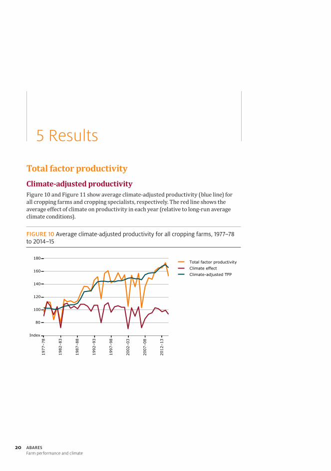
Climate-adjusted productivityFigure 10 and Figure 11 show average climate-adjusted productivity (blue line) for all cropping farms and cropping specialists, respectively. The red line shows the average effect of climate on productivity in each year (relative to long-run average climate conditions).
FIGURE 10 Average climate-adjusted productivity for all cropping farms, 1977–78 to 2014–15

5 Results
21ABARESFarm performance and climate
FIGURE 11 Average climate-adjusted productivity for cropping specialists, 1977–78 to 2014–15
After controlling for climate effects, the well-documented slowdown in productivity is apparent, with productivity growth decreasing considerably after 1993–94. However, a positive story also emerges, with evidence of a resurgence in productivity growth in recent years.
After controlling for climate, productivity growth has averaged 1.5 per cent per year since 2006–07. This productivity growth has helped the cropping sector offset the effects of a decline in average climate conditions. The results demonstrate the importance of controlling for climate when measuring agricultural productivity. These trends are difficult to observe in the underlying TFP data, given annual variability and the longer-term decline in average climate conditions.
The results suggest that the vast majority of productivity growth in the cropping sector has occurred within two key periods: 1987–88 to 1993–94 and 2007–08 to 2013–14. Together, these periods account for around 91.6 per cent of the total productivity gain between 1977–78 and 2014–15. A very similar pattern is observed for climate-adjusted wheat yields (see Figure 24).
At a regional level, the productivity rebound since 2006–07 has been strongest in the Northern GRDC region and lowest in the Western GRDC region. As observed in previous studies, cropping specialists typically out perform mixed cropping farms (Hughes et al. 2011).

5 Results
22 ABARESFarm performance and climate
TABLE 1 Average annual growth in climate-adjusted productivity for selected periods, regions and industries (%)
1977–78 to 1993–94
1993–94 to 2006–07
2006–07 to 2014–15
1977–78 to 2014–15
All cropping farms 2.09 0.16 1.50 1.28
Cropping specialists 2.46 0.16 1.74 1.49
Mixed farms 1.79 0.23 1.02 1.07
NSW 1.91 –0.28 1.82 1.11
Vic. 1.91 0.56 1.45 1.34
Qld 2.45 0.12 1.56 1.43
SA 2.42 0.30 1.30 1.43
WA 1.95 0.28 1.15 1.19
Southern 2.07 0.32 1.46 1.32
Northern 2.41 –0.15 1.69 1.35
Western 1.92 0.38 1.05 1.19
Potential drivers of productivity trendsA range of potential drivers of the productivity slowdown after 1993–94 have been identified in previous studies. For example, Sheng et al. (2011) pointed to a slowdown in the rate of growth in agricultural R&D expenditure. Jackson (2010) identified many other factors, including the loss of a profitable break crop and a shift in research priorities away from productivity enhancement.
Another potential driver is farmers’ terms of trade (the ratio of output to input prices). Previous research has shown that agricultural productivity tends to be inversely related to the terms of trade: farmers have a profit incentive to improve productivity in response to a decline in the terms of trade and vice versa (see Hughes et al. 2011, O’Donnell 2010). The significant decrease in the terms of trade for grain farms between 1980 and 1991 may have contributed to the relatively high productivity growth observed during this period (Figure 12) (see O’Donnell 2010).
FIGURE 12 Australian grain farm terms of trade, 1977–78 to 2014–15

5 Results
23ABARESFarm performance and climate
The causes of the rebound in productivity growth remain an open question. A partial explanation can be found in recent increases in farm investment (Figure 13). Average farm capital investment (in machinery and equipment and so on) has increased significantly on a per-hectare basis since 2006–07. This followed a dramatic rise in farm land prices (beginning around 2002), which helped farms to increase debt levels to finance new investment (see Martin et al. 2016). Further, increases in investment have been highest in the Northern GRDC region (where productivity gains since 2006–07 have been highest) and lowest in the Western region (where productivity gains since 2006–07 have been lowest).
FIGURE 13 Average land prices and capital investment on cropping farms, 1977–78 to 2014–15
Climate effectsFigure 14 shows the average effect of climate on TFP levels since 2000–01 relative to the period 1914–15 to 2014–15 (the annual average of the climate effect index : see Appendix B). Results for other time periods are summarised in Table 2. The results show a significant decline in climate conditions for Australian cropping farms since the mid 1990s.
The decline in conditions has been most pronounced in southern Australia, particularly in southern New South Wales and the northern parts of the Western GRDC region. Relative to the long-run average, the biggest decline has been in the Western GRDC region (8.2 per cent since 2000). However, relative to the period 1977–78 to 1993–94, the decline has been as dramatic (or worse) in southern New South Wales and Victoria (given that conditions during the period 1977–78 to 1993–94 were significantly above average in these regions).

5 Results
24 ABARESFarm performance and climate
Although the effects of climate on productivity partially reflect trends in average rainfall (as shown in Figure 3), there are some important differences. In particular, productivity in the southern high-rainfall zones of Western Australia, South Australia and Victoria has been relatively unaffected by the changes in climate since 2000; if anything, conditions have slightly improved. Given that moisture availability is less of a constraint on cropping in these regions, declines in average rainfall have had limited effect on yields and productivity. In some high-rainfall areas, it is possible that reductions in average rainfall could actually improve conditions for cropping by reducing the risk of waterlogging.
FIGURE 14 Average climate effect on productivity levels since 2000–01, relative to the 1914–15 to 2014–15 average
Climate effect on productivity2000–01 to 2014–15
>20% decrease10 to 20% decrease2 to 10% decrease<2% change2 to 10% increase>10% increase
Sparse sampleGRDC regions
5 Results
25ABARESFarm performance and climate
TABLE 2 Average annual climate effect on total factor productivity levels for selected periods, regions and industries (%)
1977–78 to 1993–94
1993–94 to 2014–15
2000–01 to 2014–15
1977–78 to 2014–15
All cropping farms 2.4 –3.2 –5.4 –0.9
Cropping specialists 2.9 –2.9 –5.7 –0.6
Mixed farms 2.1 –3.5 –5.2 –1.2
NSW 5.2 –2.8 –6.5 0.3
Vic. 4.1 –3.6 –5.3 –0.6
Qld 1.6 –4.2 –5.1 –1.4
SA 0.5 –2.4 –1.9 –1.1
WA –0.3 –3.7 –7.7 –2.5
Southern 2.9 –3.1 –5.1 –0.8
Northern 3.8 –3.0 –5.0 –0.2
Western –0.3 –4.0 –8.2 –2.6
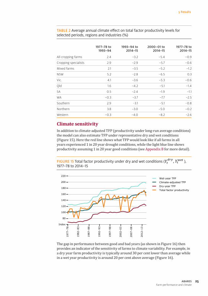
Climate sensitivityIn addition to climate-adjusted TFP (productivity under long-run average conditions) the model can also estimate TFP under representative dry and wet conditions (Figure 15). Here the red line shows what TFP would look like if all farms in all years experienced 1 in 20 year drought conditions, while the light blue line shows productivity assuming 1 in 20 year good conditions (see Appendix B for more detail).
FIGURE 15 Total factor productivity under dry and wet conditions ( , ), 1977–78 to 2014–15
The gap in performance between good and bad years (as shown in Figure 16) then provides an indicator of the sensitivity of farms to climate variability. For example, in a dry year farm productivity is typically around 30 per cent lower than average while in a wet year productivity is around 20 per cent above average (Figure 16).

5 Results
26 ABARESFarm performance and climate
FIGURE 16 Effect of dry and wet years on TFP, 1977–78 to 2014–15
As Figure 16 shows, the sensitivity of farms to climate has changed considerably over the period. During the 1980s the gap between good and bad years decreased steadily. This gap then increased during the 90s until 2005–06. Since then the gap in performance between good and bad years has closed, due largely to a reduction in sensitivity to dry conditions. By 2013–14 climate sensitivity reached a historically low level, such that a 1 in 20 drought year only reduced average productivity by around 26 per cent, compared with 37 per cent in 1979–80 (Table 3 and Table 4).
TABLE 3 Effect of dry conditions on TFP relative to long-run average conditions for selected years, regions and industries (%)
1977–78 1980–81 1989–90 2005–06 2014–15
All cropping farms –35.5 –35.8 –27.5 –33.2 –27.0
Cropping specialists –40.7 –40.8 –28.5 –35.6 –27.8
Mixed farms –32.5 –32.7 –27.1 –30.3 –26.0
NSW –38.6 –38.9 –31.8 –38.2 –29.6
Vic. –41.7 –40.3 –34.5 –36.1 –30.5
Qld –33.0 –34.4 –23.9 –30.0 –21.1
SA –40.2 –37.5 –26.2 –32.5 –28.2
WA –25.4 –29.1 –21.0 –25.5 –22.0
Southern –40.6 –39.5 –30.6 –35.7 –30.3
Northern –36.2 –34.2 –27.4 –32.7 –24.7
Western –26.0 –29.7 –21.6 –26.7 –23.2

5 Results
27ABARESFarm performance and climate
TABLE 4 Effect of wet conditions on TFP relative to long-run average conditions for selected years, regions and industries (%)
1977–78 1980–81 1989–90 2005–06 2014–15
All cropping farms 24.0 24.5 18.3 22.7 19.3
Cropping specialists 27.6 27.7 19.5 24.1 19.9
Mixed farms 21.9 22.5 17.9 21.0 18.7
NSW 24.1 25.2 20.1 25.5 20.7
Vic. 25.9 24.3 20.1 23.1 20.4
Qld 29.0 29.4 19.2 24.5 18.2
SA 27.8 26.5 18.1 22.9 20.6
WA 16.3 18.4 13.4 15.8 15.9
Southern 25.9 25.7 19.6 23.4 20.7
Northern 28.2 26.6 18.9 24.8 19.6
Western 16.3 18.3 13.7 16.2 16.5
The results suggest that a trade-off exists between productivity in good and bad years. That is, management practices that favour high productivity during good years have a tendency to increase farm exposure to negative climate shocks. This is consistent with previous observations on the Australian cropping sector during the 1990s (Stephens et al. 2011). During this period productivity gains were associated with increases in intensification (higher input use, particularly fertilisers), increased specialisation in cropping and earlier planting times. As Stephens et al. (2011) argue:
In the four southern mainland States the technology of the 1980s and 1990s was appropriate for the climate resources, but an abrupt change to a drier and more variable climate imposed severe constraints on technology which has limited yield increases. In fact, it appears that the very factors that underpinned record yield increases in the 1990s produced a cropping system that was vulnerable to the changed climate experienced in the 2000s. High rates of nitrogenous fertilisers, early sowing and higher adoption of grain legumes and oilseeds were all restricted with unfavourable conditions and record levels of yield variability. Modern cropping systems were also vulnerable to frosts, especially in southern Western Australia where frost frequency and severity appeared to increase. Consequently, the interaction between technology and climate reached record levels in the 2000s after a minimum in the 1990s.
Since the mid 2000s productivity under dry conditions has increased rapidly, helping close the gap in performance between good and bad years. The results suggest that recent innovation has focused on adapting cropping systems to the increasingly unreliable climate conditions.
As Hunt & Kirkegaard (2012) note, many recent technological and management practice changes in the sector have focused on better capturing soil moisture from summer rainfall. A key example is the adoption of no–till cropping practices, which peaked during the late 2000s (Figure 17). The regional results (Table 3 and Table 4) are consistent with a greater emphasis on summer rain, with the largest reductions in climate sensitivity occurring in NSW and Qld.—where the gains from capturing summer rain are highest—and the smallest in WA—where the gains are smallest (Hunt & Kirkegaard 2012).

5 Results
28 ABARESFarm performance and climate
FIGURE 17 Adoption of no–till cropping practices by state
Source: Llewellyn & D’emden (2010)
Decomposing climate-adjusted productivityFigure 18 shows the results of a decomposition of climate-adjusted productivity. Here the change in climate-adjusted productivity is separated into three components: time effects (related to technological change), the effects of other control variables (including AREA, LIVESTOCK and AGE) and the effect of changes in the location of sampled farms (see Appendix B).
Most of the change in climate-adjusted productivity during the period is assigned to time effects (Figure 18). The time index shows a clear pattern, with essentially all productivity gains occurring within the periods 1987–88 to 1993–94 and 2007–08 to 2013–14.
Changes in control variables (driven predominantly by scale effects) have provided consistent gains in productivity, accounting for around 16.4 per cent of total productivity growth over the period. These effects have been slightly stronger among farms in the Northern GRDC region (Figure 20). Appendix A provides more detail on the relationship between control variables and TFP. AREA typically has a positive effect on TFP except for very large farms (greater than 5,000 ha).

5 Results
29ABARESFarm performance and climate
FIGURE 18 Decomposition of climate adjusted total factor productivity, 1977–78 to 2014–15
FIGURE 19 Effect of time (technology) on total factor productivity by region, 1977–78 to 2014–15
FIGURE 20 Other (scale) effects on total factor productivity by region, 1977–78 to 2014–15

5 Results
30 ABARESFarm performance and climate
Changes in the location of cropping farms over time can effect the average productivity of the industry given differences in regional climate particularly rainfall levels. For example, if there was an increase in the number of cropping farms in ‘marginal’ lower rainfall regions this could lead to a decrease in average industry productivity and vice versa.
Figure 21 shows changes in farm sample densities for the period 2000–01 to 2014–15 relative to 1990–91 to 1999–2000. Within the farm survey, there has been a steady increase in the number of cropping farms sampled in high-rainfall zones since around 1990, particularly in south-western Victoria. There have also been decreases in some lower-rainfall areas, such as southern New South Wales and northern parts of the western cropping zone.
These changes in the location of farms with ABARES sample accounted for a small (5.1 per cent) share of the improvement in average productivity levels over the period. At a regional level, these effects have been strongest in southern Australia (Figure 23).
FIGURE 21 Change in sample density of cropping farms between 2001–2015 relative to 1990–2000
>100% increase
100% decrease
GRDC regionsSparse sample
Change in sample density2000–01 to 2014–15 relative to1989–90 to 1999–2000(farms per square km per year)

5 Results
31ABARESFarm performance and climate
FIGURE 22 Percentage change in cropping area by Statistical Local Area (SLA) between 2000-01 and 2010–11
BRS (2006b), ABARES (2016b)
Although these trends are difficult to interpret directly—given the relatively small size of the ABARES sample and changes in farm size over time—they are at least partially reflective of underlying changes in cropping activity (see Appendix C).
Appendix C presents historical data on Australian cropping areas from ABARES Land Use of Australia maps (derived from ABS Agricultural Census and surveys). The general trend since the early 1990s has been towards increased cropping at the expense of grazing. However, there have been significant changes in the distribution of cropping activity, including a shift from north to south in Victoria and Western Australia. This relative growth in cropping activity in the southern higher-rainfall zones is a long-term trend that has been driven partly by declining returns to livestock activities (following the wool price collapse) and technological innovations, such as raised bed systems (Zhang et al. 2006).

5 Results
32 ABARESFarm performance and climate
These data also show evidence of absolute declines in cropping areas in some regions since 2000–01, including parts of southern New South Wales and northern parts of the western cropping zone (Figure 22). Total cropping area in Australia increased steadily from 1992–93 to 2010–11, but has declined in the years since. While trends in the spatial distribution of cropping are affected by a range of factors—including changes in technology and commodity prices—it is likely that longer-term changes in climate are also playing a role. Ultimately, more research is required to more accurately measure land-use trends and determine their potential causes.
FIGURE 23 Farm location effect on total factor productivity by region, 1977–78 to 2014–15

5 Results
33ABARESFarm performance and climate
Wheat yields
Climate adjusted wheat yieldsAverage climate-adjusted wheat yields are shown in Figure 24 and Table 5.
FIGURE 24 Average climate-adjusted wheat yields, 1977–78 to 2014–15
Climate-adjusted yields follow a similar trend to TFP. Almost all of the improvements in wheat yields since 1977–78 have occurred within two periods: 1987–88 to 1993–94 and 2007–08 to 2013–14. Combined, these periods account for 91.1 per cent of the total productivity gain since 1977–78.
The effect of climate on wheat yield also shows a similar pattern to the effect of climate on TFP. The main difference is that wheat yields are more sensitive to climate variation than TFP. For example, reductions in total wheat yields of up to 50 per cent (relative to long-run average climate conditions) are observed in the worst drought years, compared with around 25 per cent for TFP.
At a regional level, the Western GRDC region outperformed all other areas in terms of growth in climate-adjusted wheat yields between 1977–78 and 2006–07. However, the Southern GRDC region has experienced the highest growth since 2006–07, at 2.9 per cent per year.

5 Results
34 ABARESFarm performance and climate
TABLE 5 Average annual growth in climate-adjusted wheat yields wheat yields for selected periods, regions and industries (%)
1977–78 to 1993–94
1993–94 to 2006–07
2006–07 to 2014–15
1977–78 to 2014–15
All cropping farms 1.58 0.01 2.56 1.24
Cropping specialists 1.61 0.17 2.73 1.34
Mixed farms 1.78 –0.40 2.24 1.11
NSW 1.24 –0.24 3.00 1.10
Vic. 1.49 –0.75 2.90 1.00
Qld 0.77 –0.24 2.87 0.86
SA 2.79 –0.56 2.80 1.60
WA 2.33 0.29 2.16 1.57
Southern 1.56 –0.47 2.93 1.14
Northern 0.93 –0.21 2.72 0.91
Western 2.33 0.28 2.08 1.55
Climate effectsFigure 25 and Table 6 show the effect of climate conditions since 2000–01 on wheat yields relative to long-run average conditions (the average of the climate effect index
since 2000–01). The trends here are similar to TFP, with a significant decline in conditions since 2000–01 (11.9 per cent relative to the long-run average).
Again, the largest effects (relative to the long-run average) have occurred in Western Australia, although the declines in south-eastern Australia have been more dramatic relative to the period 1977–78 to 1993–94. Relative to the TFP results, the wheat yield map shows a more positive effect of climate since 2000–01 in parts of northern New South Wales.
FIGURE 25 Average climate effect on wheat yield levels since 2000–01, relative to 1914–15 to 2014–15
Climate effect on wheat yield2000–01 to 2014–15
>20% decrease10 to 20% decrease2 to 10% decrease<2% change2 to 10% increase>10% increase
Sparse sampleGRDC regions

5 Results
35ABARESFarm performance and climate
TABLE 6 Average annual climate effect on wheat yields, , for selected periods, regions and industries (%)
1977–78 to 1993–94
1993–94 to 2014–15
2000–01 to 2014–15
1977–78 to 2014–15
All cropping farms 2.6 –6.1 –11.9 –3.0
Cropping specialists 2.1 –6.1 –12.4 –3.2
Mixed farms 2.9 –6.1 –10.9 –2.8
NSW 6.9 –3.2 –9.7 0.0
Vic. 10.3 –10.3 –14.8 –2.3
Qld 2.9 –5.6 –6.2 –1.3
SA 2.3 –4.4 –5.6 –1.9
WA –3.5 –8.2 –16.3 –6.8
Southern 5.7 –6.3 –10.9 –1.9
Northern 5.8 –0.9 –3.0 1.6
Western –3.6 –8.3 –16.5 –6.9
Climate sensitivityAs would be expected, wheat yields are more sensitive to climate variation than TFP. However, the results also suggest that the sensitivity of wheat yields to climate has decreased significantly in recent years, particularly in 2011–12 (Figure 26). Similar to TFP, this recent reduction in sensitivity has been strongest in New South Wales and Queensland (Table 7 and Table 8). This may be related to the higher summer rainfall in these areas, which offers greater gains from moisture conserving management practices.
FIGURE 26 Effect of dry and wet years on wheat yields, 1977–78 to 2014–15

5 Results
36 ABARESFarm performance and climate
TABLE 7 Effect of dry conditions on wheat yield relative to long-run average conditions for selected years, regions and industries
1977–78 1980–81 1989–90 2005–06 2014–15
All cropping farms –59.3 –56.9 –50.6 –55.5 –43.0
Cropping specialists –63.7 –60.9 –54.4 –56.3 –42.2
Mixed farms –53.6 –51.6 –48.6 –53.5 –45.0
NSW –63.5 –61.4 –60.6 –64.4 –48.9
Vic. –62.3 –61.7 –59.1 –60.9 –47.2
Qld –50.6 –51.9 –50.4 –55.6 –40.2
SA –63.1 –60.9 –52.3 –58.0 –43.5
WA –54.8 –51.6 –43.0 –46.5 –38.3
Southern –64.3 –63.3 –57.0 –61.0 –47.6
Northern –57.8 –56.0 –55.1 –62.5 –42.6
Western –54.9 –51.8 –43.0 –46.6 –38.7
TABLE 8 Effect of wet conditions on wheat yield relative to long-run average conditions for selected years, regions and industries
1977–78 1980–81 1989–90 2005–06 2014–15
All cropping farms 44.6 43.4 36.0 44.8 35.8
Cropping specialists 48.3 45.9 39.5 45.5 34.9
Mixed farms 39.8 40.0 34.1 43.2 37.9
NSW 50.0 49.0 46.8 54.1 39.1
Vic. 44.3 45.5 38.8 52.5 44.3
Qld 50.7 52.6 46.7 52.7 38.4
SA 56.0 52.7 40.5 52.5 39.3
WA 35.7 34.0 25.4 31.2 29.7
Southern 49.5 49.2 42.1 52.5 41.1
Northern 50.5 50.5 46.9 56.8 37.7
Western 35.7 34.1 25.5 31.3 30.0

5 Results
37ABARESFarm performance and climate
Decomposing climate-adjusted wheat yieldFigure 27 shows the decomposition of climate-adjusted wheat yields. Again, the change in climate-adjusted productivity is separated into three components: time effects (related to technological change) the effects of other control variables (including AREA, LIVESTOCK and AGE) and the effect of changes in the location of sampled farms (see Appendix B). The vast majority of improvements in wheat yield are assigned to time (technology) effects. Farm location changes had a small positive effect on productivity between 1989–90 and 2014–15, while other (i.e., scale) effects have been minimal. The limited effect of farm size is expected here, given that the benefits of increasing farm scale tend to be cost savings (i.e. reduced capital, labour, materials) rather than higher yields.
FIGURE 27 Decomposition of climate adjusted wheat yield, 1977–78 to 2014–15
38 ABARESFarm performance and climate
6 Future research
The models developed in this study have a range of potential future applications and extensions as detailed below.
Monitoring productivity changeIn future, the ability of cropping farms to continue adapting to climate change will be crucial to the success of the industry. Much of this adaptation will involve ‘incremental’ improvements in technology driven by existing agricultural R&D systems. In the longer term, more ‘transformational’ adaptation could occur, including changes in land use.
In both cases, understanding the effects of climate on farm productivity will be important. Given the potential for significant changes in the future climate, productivity estimates that isolate climate effects will become necessary for assessing the performance of agricultural research, development and extension systems, and helping to guide future investment decisions. Further, given the large uncertainties surrounding any long-run change in land use, it will be important to monitor climate trends and their effects on farm productivity and profitability, and land use as they gradually unfold.
Informing risk management systemsWith growing climate variability, farm risk management systems—including government drought assistance programmes and private insurance products—will become increasingly important for the cropping sector.
Typically, government drought assistance programmes (at least those providing direct financial assistance to farm businesses) require an assessment of climatic impacts to determine the eligibility of individual farms. Although the previous system of regional ‘exceptional circumstances’ declarations that applied during the 1990s and 2000s is no longer in place, some Australian Government programmes still link eligibility to climate statistics. For example, Drought Assistance Concessional Loans, and eligibility for early withdrawal of funds from Farm Management Deposit accounts, both include eligibility criteria based on a 1 in 20 year rainfall deficiency.

6 Future research
39ABARESFarm performance and climate
As previous studies have argued (Nelson et al. 2007), simple climate statistics provide an incomplete measure of drought effects, given the complex relationships between climate variables, and farm productivity and profitability. Farm-level estimates of the effect of climate on productivity or profitability—derived using methods similar to those used in this study—could potentially provide more accurate drought effect indicators.
This type of information could also help with the development of drought insurance products. A commonly cited constraint on the development of private crop insurance markets is a lack of detailed farm-level data on the effect of climate on farm revenue and costs, which are necessary to price insurance contracts (Deloitte Access Economics 2015). Here, there may be a role for government in providing data and models to measure the effect of climate on farms (similar to the Australian Government’s National Flood Risk Information Project), to support the development of private crop insurance markets.
Analysing larger data setsAlthough the methods applied in this study proved effective, they are better suited to larger datasets. A key area for future research is applying these methods to ABS Agricultural Census data. In addition to providing more precise results, ABS census data would provide more complete regional coverage and a greater range of crop types. Census data could also provide a better indication of changes in the spatial distribution of cropping areas over time.
From productivity to profitAnother option is to extend the analysis beyond TFP and crop yields to consider the effect of climate on costs, revenues and profits. Here, ABARES farm survey data could be used to develop a farm income simulation model. The model could use similar regression methods to predict farm inputs and outputs (and costs and revenues), given climate conditions, and prevailing output and input prices. This approach would provide a more complete understanding of farm-level responses to climate variability.
Further, profit measures would provide a better indicator of future land-use change. For example, a farm income model could be used to simulate the long-term effect of climate change on farm profitability based on the latest climate projections.
40 ABARESFarm performance and climate
Appendix A: Machine learning methods
Estimates of changes in farm profit due to climate change could help to identify those regions, industries and farm types facing the greatest adaptation pressure.
Gradient-boosted regression treesThis study uses two popular ‘regression tree’ based machine learning methods: ‘random forests’ (Breiman 2001) and ‘gradient-boosted regression trees’ (GBRT) (Friedman 2002). Similar to random forests (Breiman 2001), GBRT is an ensemble method that combines a large number of simple regression tree models. Large scale empirical testing has found that well calibrated GBRT models consistently outperform other common machine learning algorithms, including random forests (Caruana & Niculescu-Mizil 2006). This study usess the random forest and GBRT methods implemented in the Python machine learning software package scikit-learn (Pedregosa et al. 2011).
Cross-validationCross-validation involves fitting a regression model to a subset of the available data (the training set) and then measuring the performance (the prediction error) on the withheld data (the testing set). Cross-validation provides a more reliable measure of performance than in-sample fit measures (such as simple ), particularly for non-parametric regression models.
In this study, 10-fold cross-validation is used. Here, the data are divided into 10 sub-samples. At each step, 9 of the samples are used to fit the model and 1 is withheld as the testing set. This process is repeated 10 times, so that each sub sample is used for testing data once. The final score (cross-validated ) is taken as the mean of the scores from each sub-sample.
Feature selectionThis study uses a recursive feature elimination method to select an appropriate subset of climate variables for each model. The process begins by estimating the model with the full set of climate variables. The performance of the model is assessed by cross-validation, and the climate variables with the lowest importance values (the bottom 5th percentile) are eliminated. This process is repeated 10 times. The final set of climate variables is the one that achieves the highest cross-validated performance score.

Appendix A: Machine learning methods
41ABARESFarm performance and climate
The most important climate variables in the final cropping and livestock models are shown in Figure 28 and Figure 29. In both models, the most important climate variable is WINTER_RAIN.
FIGURE 28 Climate variable importance rankings TFP model
FIGURE 29 Climate variable importance rankings W_YIELD model

Appendix A: Machine learning methods
42 ABARESFarm performance and climate
Meta-parametersGBRT models involve a number of key meta-parameters that need to be ‘tuned’ to maximise performance, including the number of samples per split, the learning rate and the number of trees to estimate. A search of the meta-parameter space was completed, as summarised in Figure 30. The final meta-parameters are those that maximise the cross-validated performance of the model (Table 9).
TABLE 9 Final meta-parameter values
TFP W_YIELD
Number of samples per split 50 5
Number of trees 1,175 1,475
Learning rate 0.045 0.032
FIGURE 30 Model estimation process
Meta-parameter selectionSelect new meta-parameter values(repeat)
Feature selectionSelect most important climate variables(repeat 10 times)
Cross – validationSelect train and test data sets(repeat 10 times)
Meta-parameters
Selected features
Train / test modelFit model to training setEvaluate on test set
Train / test data sets
Score
Average score
Max. score
Model testingFigure 31 shows the cross-validated performance of the GBRT and random forest methods, against a benchmark quadratic regression model fit by ordinary least squares, taking the form:
where are parameters and includes: WINTER_RAIN, SUMMER_RAIN, SUMMER_LAG_RAIN, WINTER_TMAX, SUMMER_TMAX, WINTER_TMIN, SUMMER_TMIN, YEAR, LAT, LONG, AREA, AGE and LIVESTOCK.

Appendix A: Machine learning methods
43ABARESFarm performance and climate
On this basis, GBRT was selected as the preferred regression method.
FIGURE 31 Model performance (cross-validated )
Although these cross–validated scores may seem low, they need to be considered in context. The farm-level data used in this study are subject to a high degree of heterogeneity and noise. The productivity levels of individual farms can vary for a range of non–climate related factors external to the model (see Kokic et al. 2006). When the model predictions are compared at an aggregate or regional level, the model accounts for a very high proportion of annual variation (see Figure 32).
FIGURE 32 National average annual total factor productivity predicitions (in–sample), 1977–78 to 2014–15
Appendix A: Machine learning methods
44 ABARESFarm performance and climate
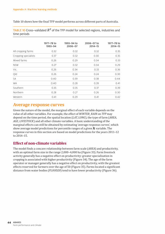
Table 10 shows how the final TFP model performs across different parts of Australia.
TABLE 10 Cross–validated of the TFP model for selected regions, industries and time periods
1977–78 to 1993–94
1993–94 to 2006–07
2006–07 to 2014–15
1977–78 to 2014–15
All cropping farms 0.32 0.32 0.32 0.35
Cropping specialists 0.37 0.32 0.30 0.35
Mixed farms 0.26 0.29 0.34 0.33
NSW 0.27 0.32 0.34 0.29
Vic. 0.26 0.34 0.33 0.36
Qld 0.26 0.24 0.24 0.30
SA 0.40 0.39 0.38 0.44
WA 0.40 0.28 0.39 0.41
Southern 0.35 0.35 0.37 0.39
Northern 0.28 0.27 0.26 0.30
Western 0.41 0.29 0.41 0.42
Average response curvesGiven the nature of the model, the marginal effect of each variable depends on the value of all other variables. For example, the effect of WINTER_RAIN on TFP may depend on the time period, the spatial location (LAT, LONG), the type of farm (AREA, AGE, LIVESTOCK) and all other climate variables. A basic understanding of the marginal effects can still be obtained by estimating ‘average response curves’, which show average model predictions for percentile ranges of a given variable. The response curves in this section are based on model predictions for the years 2011–12 to 2014–15.
Effect of non-climate variablesThe model finds a concave relationship between farm scale (AREA) and productivity, with an optimal farm size in the range 2,000–4,000 ha (Figure 33). Farm livestock activity generally has a negative effect on productivity: greater specialisation in cropping is associated with higher productivity (Figure 34). The age of the farm operator or manager generally has a negative effect on productivity, with the greatest effects reserved for farmers over the age of 50 (Figure 35). Farms located a significant distance from water bodies (FLOOD20) tend to have lower productivity (Figure 36).

Appendix A: Machine learning methods
45ABARESFarm performance and climate
FIGURE 33 Average response of climate-adjusted TFP to AREA
FIGURE 34 Average response of climate-adjusted TFP to LIVESTOCK
FIGURE 35 Average response of climate-adjusted TFP to AGE

Appendix A: Machine learning methods
46 ABARESFarm performance and climate
FIGURE 36 Average response of climate-adjusted TFP to FLOOD20
The wheat yield model finds a negative correlation between wheat area planted and yield (Figure 37).
FIGURE 37 Average response of climate-adjusted W_YIELD to W_AREA
In the wheat yield model, the variable FLOOD1_5 acts as an indicator of farm exposure to flooding. In wet years, close proximity to a flood-prone area has a negative effect on yield, whereas in dry years it has a positive effect (Figure 38).
Appendix A: Machine learning methods
47ABARESFarm performance and climate
FIGURE 38 Average response of predicted W_YIELD to FLOOD1_5
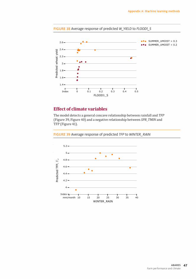
Effect of climate variablesThe model detects a general concave relationship between rainfall and TFP (Figure 39, Figure 40) and a negative relationship between SPR_TMIN and TFP (Figure 41).
FIGURE 39 Average response of predicted TFP to WINTER_RAIN

Appendix A: Machine learning methods
48 ABARESFarm performance and climate
FIGURE 40 Average response of predicted TFP to TWO_YEAR_LAG_RAIN
FIGURE 41 Average response of predicted TFP to SPR_RAIN
The model detects positive relationships between rainfall and W_YIELD (Figure 42, Figure 43), and negative relationships between temperatures and W_YIELD (Figure 44, Figure 45).
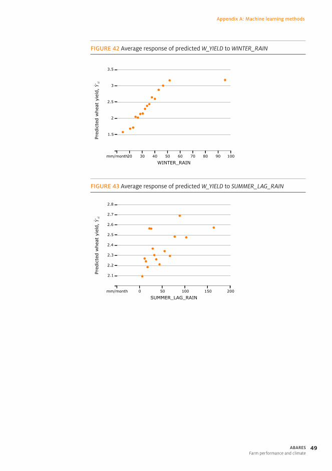
Appendix A: Machine learning methods
49ABARESFarm performance and climate
FIGURE 42 Average response of predicted W_YIELD to WINTER_RAIN
FIGURE 43 Average response of predicted W_YIELD to SUMMER_LAG_RAIN

Appendix A: Machine learning methods
50 ABARESFarm performance and climate
FIGURE 44 Average response of predicted W_YIELD to WIN_TMAX
FIGURE 45 Average response of predicted W_YIELD to SPR_TMIN

51ABARESFarm performance and climate
Appendix B: Calculating climate-adjusted productivity
This study involves estimating regression models of the form:
where is the farm performance measure (TFP or W_YIELD) for farm in period , is a vector of farm specific-climate variables, a vector of farm characteristics
and is an unknown function.
Once an estimate for the function is obtained, we can generate predictions of farm performance measures under differing climate conditions:
Here, is an estimate of what farm performance would have been for farm under the climate conditions of a given year .
Climate adjusted productivityThis type of counter factual prediction, can be used to isolate the effects of climate variation for particular years. In particular, we can define climate-adjusted productivity :
That is, we predict farm performance for each observation under the climate conditions prevailing for each of the past 101 years, then take the average across those 101 years. is then a measure of the performance of farm in period under long-run average climate conditions for that location. Note that controls for temporal variation in climate (annual variability and climate change) but does not attempt to control for persistent spatial differences in climate.

Appendix B: Calculating climate-adjusted productivity
52 ABARESFarm performance and climate
In addition, we define and as the 5th and 95th percentiles of for each observation. and measure the performance of farms under unfavourable or favourable conditions, respectively whereas measures performance under average conditions.
Climate effectsNext we define the climate effect index as:
Here measures the total effect of climate on the productivity of farm for year relative to long-run average conditions.
For each observation, we also define as the effect of year climate conditions on farm in year . We also define and as the 5th and 95th percentiles of for each observation less 100 (to reflect the difference relative to long-run average conditions). , for example, is a measure of the sensitivity of a farm to adverse climate conditions (that is, the percentage effect on TFP of a 1-in-20 year drought). Given the nature of the model this sensitivity to climate can change over time.
Calculating averagesIn the results section, farm-level estimates are presented mostly as simple annual averages for example:
Note that sample average TFP estimate differ slightly from the TFP indexes regularly produced by ABARES (where individual farm-level inputs and outputs are combined using index number methods to produce an aggregate industry TFP series).
In contrast, wheat yield results are presented as weighted averages where each farm observation is weighted by both the area planted (W_AREA) and the farm survey weight.
Decomposing climate-adjusted productivityThe estimated models can be used to decompose climate-adjusted productivity further, to isolate the effect of technology change, (time ), the effect of changes in the spatial distribution of sampled farms (spatial coordinates LAT and LONG) and the effect changes in farm control variables (including, farm land area—AREA, the extent of grazing activity—LIVESTOCK and farmer age—AGE).
To do this, two alternative sets of model predictions are generated, one where the year is held constant (at 2015):

Appendix B: Calculating climate-adjusted productivity
53ABARESFarm performance and climate
Here, predicts the productivity of each farm in each year climate conditions, but with 2015 technology. The other set of predictions holds both the year (technology) and other farm control variables (AREA, LIVESTOCK, AGE) constant:
Here is as defined previously, but with AREA, LIVESTOCK and AGE for each farm replaced with a long-run average value. For AGE, the long-run average value is simply the sample mean. For the other variables, the long-run average value is location specific, based on a model fit by GBRT (against just LAT and LONG).
Indexes are generated for these new sets of predictions following the method described above. The effects of changes in farm location (SPACE) are given by the
sample average of (where the only variables allowed to change over time are LAT and LONG), the effects of other farm controls (OTHER—including AREA, LIVESTOCK, AGE etc.) and technological change (TIME) defined as:

54 ABARESFarm performance and climate
Appendix C: Changes in Australian cropping areas
Trends in Australian agricultural land-use will be described further in a forthcoming ABARES report National reporting on agricultural land use change in Australia, which will present detailed information on agricultural land use based on ABARES Land Use of Australia maps and ABS Agricultural Census data. In particular, the report presents concorded agricultural data for all census years between 1992–93 and 2010–11 using a consistent set of region (Statistical Local Area—SLA) and industry definitions. Similar data are also available on an annual basis for the years 1982–83 to 2009–10 at the higher Statistical District (SD) regional level. This section highlights some key trends using these two data sets.
Figure 46 shows total Australian crop areas relative to total agricultural land since 1992–93. During this time there has been a general shift towards cropping and away from grazing, driven in part by declining livestock returns following the collapse of the wool reserve price scheme. However, the trend towards increasing crop area appears to have reversed in recent years, with a declining trend between 2010–11 and 2014–15.
FIGURE 46 Total Australian cropping area and total agricultural area, 1992–93 to 2014–15
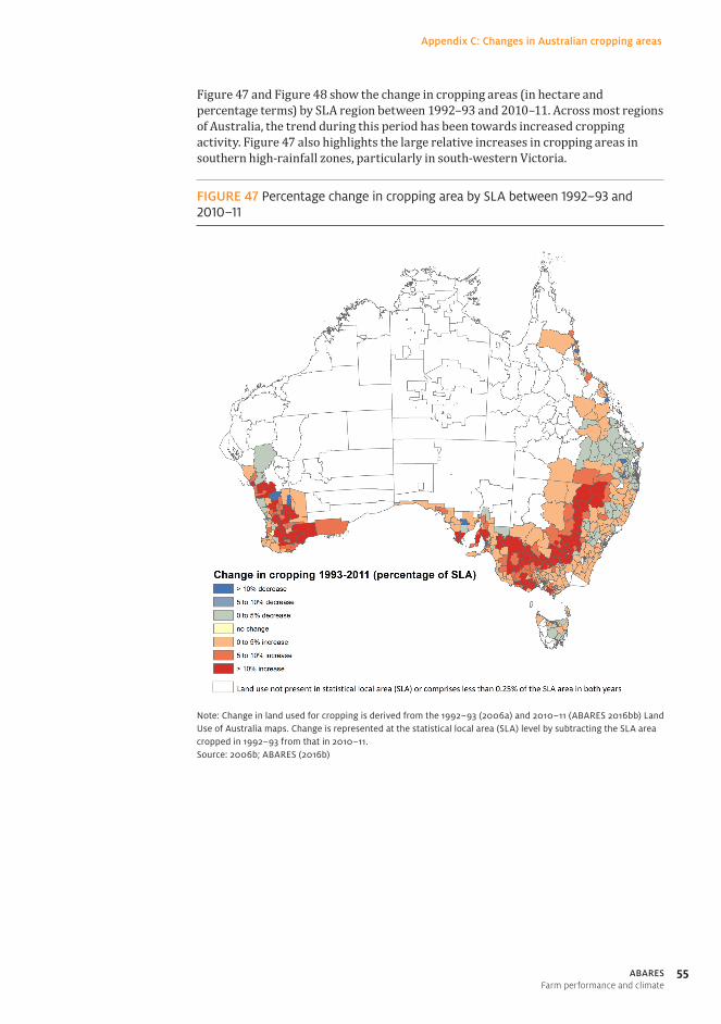
Appendix C: Changes in Australian cropping areas
55ABARESFarm performance and climate
Figure 47 and Figure 48 show the change in cropping areas (in hectare and percentage terms) by SLA region between 1992–93 and 2010–11. Across most regions of Australia, the trend during this period has been towards increased cropping activity. Figure 47 also highlights the large relative increases in cropping areas in southern high-rainfall zones, particularly in south-western Victoria.
FIGURE 47 Percentage change in cropping area by SLA between 1992–93 and 2010–11
Note: Change in land used for cropping is derived from the 1992–93 (2006a) and 2010–11 (ABARES 2016bb) Land Use of Australia maps. Change is represented at the statistical local area (SLA) level by subtracting the SLA area cropped in 1992–93 from that in 2010–11. Source: 2006b; ABARES (2016b)

Appendix C: Changes in Australian cropping areas
56 ABARESFarm performance and climate
FIGURE 48 Absolute change in cropping area by SLA between 1992–93 and 2010–11
Note: Change in land used for cropping derived from the 1992-93 (2006a) and 2010-11 (ABARES 2016b) Land Use of Australia maps. Change is represented at the statistical local area (SLA) level by subtracting the SLA area cropped in 1992-93 from that in 2010-11. Source: 2006b; ABARES (2016b)
Figure 49 and Figure 50 show the change (percentage and hectare terms) in cropping areas by SLA region between 2000–01 and 2010–11. While the long–term trend since the early 90s has been towards increased cropping activity the more recent trends since 2000–01 are mixed. Here we can see some evidence of declining crop areas in certain regions, including northern parts of the Western Australian cropping zone and in parts of southern NSW. These recent declines in land use are somewhat consistent with the farm survey data presented in this report (see Figure 21).

Appendix C: Changes in Australian cropping areas
57ABARESFarm performance and climate
FIGURE 49 Percentage change in cropping area by SLA region between 2000–01 to 2010–11
Note: Change in land used for cropping is derived from the 2000–01 (2006a) and 2010–11 (ABARES 2016b) Land Use of Australia maps. Change is represented at the SLA level by subtracting the SLA area cropped in 2000–01 from that in 2010–11. Source: 2006b; ABARES (2016b)

Appendix C: Changes in Australian cropping areas
58 ABARESFarm performance and climate
FIGURE 50 Absolute change in cropping area by SLA region between 2000–01 and 2010–11
Note: Change in land used for cropping is derived from the 2000–01 (2006a) and 2010–11 (ABARES 2016b) Land Use of Australia maps. Change is represented at the SLA level by subtracting the SLA area cropped in 2000–01 from that in 2010–11. Source: 2006b; ABARES (2016b)
Annual data at the SD region level provide a clearer picture of some of these land use trends, particularly the shift towards increased cropping in southern high rainfall zones in Western Australia and Victoria. Figure 51 shows the relevant SD region boundaries.

Appendix C: Changes in Australian cropping areas
59ABARESFarm performance and climate
FIGURE 51 2006 Statistical District (SD) region boundaries
Figure 52 shows annual cropping areas by region in Western Australia between 1982–83 and 2009–10. Figure 53 shows the proportions of Western Australian cropping area grown in selected regions. Since the early 1990s total cropping areas in Western Australia have grown steadily. Behind this increasing trend has been a redistribution of total cropping activity southwards.
Figure 53 shows that the proportion of crops grown in the southern part of the Western Australian cropping belt (Lower Great Southern and South Eastern) has been increasing, while the share of the northern part (Central) has declined. This trend appears to have accelerated in recent times. Total cropping area in the Central region remained steady during the 10 years from 1999 to 2000 at around 1 million hectares (other than a dip during the 2006–07 drought). Cropping areas in the south (Lower Great Southern plus South Eastern) increased from around 1.3 million to 2 million hectares over the same period.
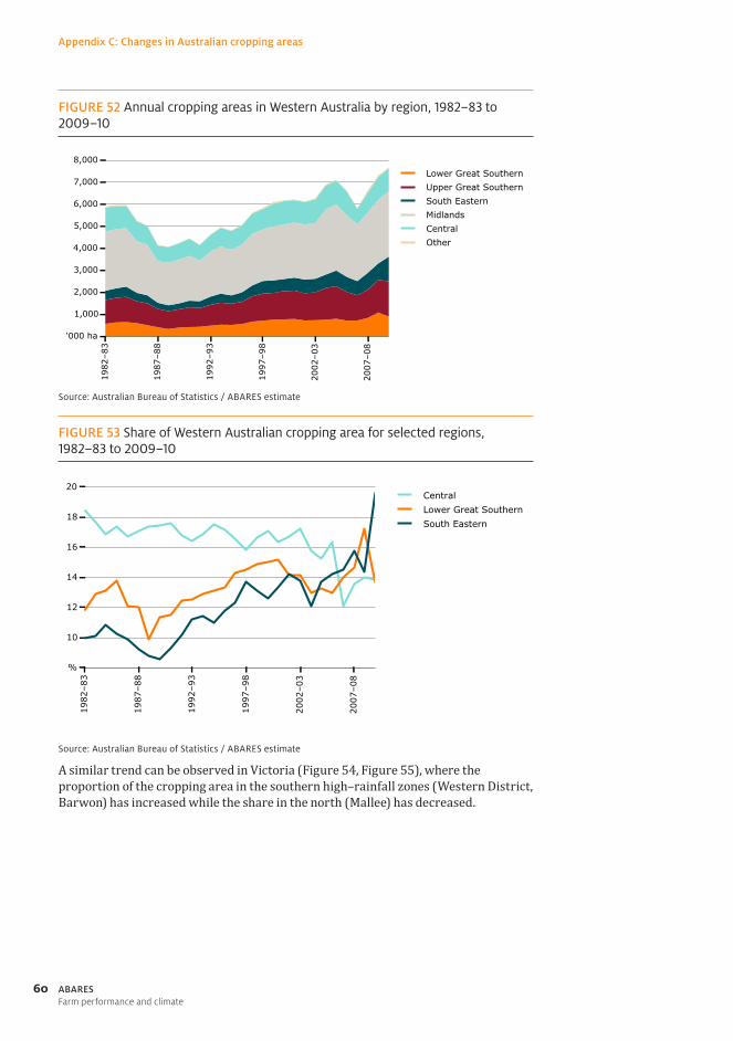
Appendix C: Changes in Australian cropping areas
60 ABARESFarm performance and climate
FIGURE 52 Annual cropping areas in Western Australia by region, 1982–83 to 2009–10
Source: Australian Bureau of Statistics / ABARES estimate
FIGURE 53 Share of Western Australian cropping area for selected regions, 1982–83 to 2009–10
Source: Australian Bureau of Statistics / ABARES estimate
A similar trend can be observed in Victoria (Figure 54, Figure 55), where the proportion of the cropping area in the southern high–rainfall zones (Western District, Barwon) has increased while the share in the north (Mallee) has decreased.
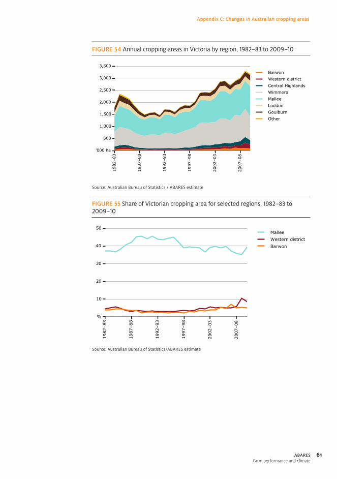
Appendix C: Changes in Australian cropping areas
61ABARESFarm performance and climate
FIGURE 54 Annual cropping areas in Victoria by region, 1982–83 to 2009–10
Source: Australian Bureau of Statistics / ABARES estimate
FIGURE 55 Share of Victorian cropping area for selected regions, 1982–83 to 2009–10
Source: Australian Bureau of Statistics/ABARES estimate

62 ABARESFarm performance and climate
References
Alexander, F & Kokic, P 2005, Productivity in the Australian grains industry, Australian Bureau of Agricultural and Resource Economics and Sciences, Canberra.
ABARES 2016a, Catchment scale land use of Australia, Australian Bureau of Agricultural and Resource Economics and Sciences, Canberra.
ABARES 2016b, Land use of Australia, 2010–11, Australian Bureau of Agricultural and Resource Economics and Sciences, Canberra.
ABARES 2016c, Australian farm survey results 2013–14 to 2015–16, Australian Bureau of Agricultural and Resource Economics and Sciences, Canberra, data.daff.gov.au/data/warehouse/9aas/FarmSurveyResults/2016/FarmSurveyResults2016_V1.1.0.pdf.
AEGIC 2016, ‘New Australian climate developing’, Australian Export Grains Innovation Centre, Perth, aegic.org.au/new-australian-climate-developing/.
Breiman, L 2001, ‘Random forests’, Machine Learning, vol. 45, no. 1, pp. 5–32.
BRS 2006a, Land use of Australia, Version 3, 1992–93, Bureau of Rural Sciences, Canberra. data.daff.gov.au/anrdl/metadata_files/pa_luav3g9abl_03012a01.xml
BRS 2006b, Land use of Australia, Version 3, 2000-01, Bureau of Rural Sciences, Canberra. data.daff.gov.au/anrdl/metadata_files/pa_luav3g9abl_03012a05.xml
Cai, W & Cowan, T 2008, ‘Dynamics of late autumn rainfall reduction over southeastern Australia’, Geophysical Research Letters, vol. 35, no. 9.
Cai, W, Cowan, T & Thatcher, M 2012, ‘Rainfall reductions over Southern Hemisphere semi-arid regions: the role of subtropical dry zone expansion’, Scientific Reports, vol. 2, p. 702.
Caruana, R & Niculescu-Mizil, A 2006, ‘An empirical comparison of supervised learning algorithms’, in Proceedings of the 23rd International Conference on Machine Learning, Association for Computing Machinery, New York, pp. 161–8.
Che, N, Kompas, T, Xayavong, V & Cook, D 2012, ‘Profitability, productivity and the efficiency of grain production with climate impacts: a case study of Western Australia’, Crawford School Research Paper, no. 12-08.

References
63ABARESFarm performance and climate
CSIRO 2012, ‘Climate and water availability in south-eastern Australia: a synthesis of findings from Phase 2 of the South Eastern Australian Climate Initiative (SEACI)’, Commonwealth Scientific and Industrial Research Organisation, seaci.org/publications/documents/SEACI-2Reports/SEACI_Phase2_SynthesisReport.pdf.
CSIRO & BoM 2015, Climate change in Australia: projections for Australia’s NRM regions, Commonwealth Scientific and Industrial Research Organisation & Bureau of Meteorology, climatechangeinaustralia.gov.au/media/ccia/2.1.6/cms_page_media/168/CCIA_2015_NRM_TechnicalReport_WEB.pdf.
CSIRO & BoM 2016, State of the climate, Commonwealth Scientific and Industrial Research Organisation & Bureau of Meteorology, bom.gov.au/state-of-the-climate/State-of-the-Climate-2016.pdf.
Deloitte Access Economics 2015, Scoping study on multi-peril insurance and its application to Agricultural Industries in NSW, Deloitte Access Economics.
Friedman, JH 2002, ‘Stochastic gradient boosting’, Computational Statistics & Data Analysis, vol. 38, no. 4, pp. 367–78.
Ghahramani, A, Kokic, PN, Moore, AD, Zheng, B, Chapman, SC, Howden, MS & Crimp, SJ 2015, ‘The value of adapting to climate change in Australian wheat farm systems: farm to cross-regional scale’, Agriculture, Ecosystems & Environment, vol. 211, pp. 112–25.
Gunasekera, D, Ford, M & Tulloh, C 2007a, ‘Climate change: issues and challenges for Australian agriculture and forestry’, Australian Commodities, no. 3, pp. 493–515.
Gunasekera, D, Kim, Y, Tulloh, C & Ford, M 2007b, ‘Climate change: impacts on Australian agriculture’, Australian Commodities: Forecasts and Issues, vol. 14, no. 4, p. 657.
Heyhoe, E, Kim, Y, Kokic, P, Levantis, C, Helal, A, Schneider, K, Crimp, S, Nelson, R, Flood, N & Carter, J 2007, ‘Adapting to climate change: issues and challenges in the agriculture sector’, Australian Commodities: Forecasts and Issues, vol. 14, no. 1, p. 167.
Hochman, Z, Gobbert, D & Horan, H 2017, ‘Climate trends account for stalled wheat yields in Australia since 1990’, Global Change Biology, vol. 5.
Holzworth, DP, Huth, NI, deVoil, PG, Zurcher, EJ, Herrmann, NI, McLean, G, Chenu, K, van Oosterom, EJ, Snow, V, Murphy, C, Moore, AD, Brown, H, Whish, JPM, Verrall, S, Fainges, J, Bell, LW, Peake, AS, Poulton, PL, Hochman, Z, Thorburn, PJ, Gaydon, DS, Dalgliesh, NP, Rodriguez, D, Cox, H, Chapman, S, Doherty, A, Teixeira, E, Sharp, J, Cichota, R, Vogeler, I, Li, FY, Wang, E, Hammer, GL, Robertson, MJ, Dimes, JP, Whitbread, AM, Hunt, J, van Rees, H, McClelland, T, Carberry, PS, Hargreaves, JNG, MacLeod, N, McDonald, C, Harsdorf, J, Wedgwood, S & Keating, BA 2014, ‘APSIM: evolution towards a new generation of agricultural systems simulation’, Environmental Modelling & Software, vol. 62, pp. 327–50.
Hughes, N, Lawson, K, Davidson, A, Jackson, T, Sheng, Y 2011, ‘Productivity pathways: climate adjusted production frontiers for the Australian broadacre cropping industry’, Australian Bureau of Agricultural and Resource Economics and Sciences, Canberra. data.daff.gov.au/data/warehouse/pe_abares99001781/CP11.05_Broadacre_crop.pdf.

References
64 ABARESFarm performance and climate
Hunt, J & Kirkegaard, J 2012, ‘Re-evaluating the contribution of summer fallow rain to wheat yield in southern Australia’, Crop & Pasture Science, vol. 62, no. 11, pp. 915–29 .
IPCC (Intergovernmental Panel on Climate Change) 2014, Climate change 2014: impacts, adaptation and vulnerability. Part B: Regional aspects, Cambridge University Press.
Islam, N, Xayavong, V, Kingwell, R, Anderton, L, Feldman, D 2014, ‘Farm productivity in an Australian region affected by a changing climate’, in Proceedings of the 58th Annual Conference of the Australian Agricultural and Resource Economics Society, Port Macquarie, 4–7 February, Australian Agricultural and Resource Economics Society, Canberra.
Jackson, T 2010, Harvesting productivity: ABARE–GRDC workshops on grains productivity growth, Australian Bureau of Agricultural and Resource Economics, Canberra, data.daff.gov.au/data/warehouse/pe_abarebrs99014452/harvesting_prod.pdf.
Keating, BA, Carberry, PS, Hammer, GL, Probert, ME, Robertson, MJ, Holzworth, D, Huth, NI, Hargreaves, JNG, Meinke, H, Hochman, Z, McLean, G, Verburg, K, Snow, V, Dimes, JP, Silburn, M, Wang, E, Brown, S, Bristow, KL, Asseng, S, Chapman, S, McCown, RL, Freebairn, DM & Smith, CJ 2003, ‘An overview of APSIM, a model designed for farming systems simulation’, European Journal of Agronomy, vol. 18, no. 3, pp. 267–88.
Keogh, M 2012,‘Including risk in enterprise decisions in Australia’s riskiest businesses’, in Proceedings of the 56th Annual Conference of the Australian Agricultural and Resource Economics Society, Perth, Australian Agricultural and Resource Economics Society, Canberra, pp. 8–10.
Kingwell, R, Anderton, L, Islam, N, Xayavong, V, Wardell-Johnson, A, Feldman, D & Speijers, J 2014, ‘Broadacre farmers adapting to a changing climate’, Applied Studies in Climate Adaptation, p. 130.
Kokic, P, Davidson, A & Boero Rodriguez, V 2006, ‘Australia’s grains industry: factors influencing productivity growth’, Australian Commodities: Forecasts and Issues, vol. 13, no. 4, p. 705.
Kokic, P, Heaney, A, Pechey, L, Crimp, S & Fisher, BS 2005, ‘Climate change: predicting the impacts on agriculture: a case study’, Australian Commodities: Forecasts and Issues, vol. 12, no. 1, p. 161.
Llewellyn, R & D’emden, F 2010, Adoption of no-till cropping practices in Australian grain growing regions, Grains Research and Development Corporation, Canberra.
Martin, P, Gray, E & Thompson, T 2014, Australian grains: financial performance of grain producing farms 2011–12 to 2013–14, Australian Bureau of Agricultural and Resource Economics and Sciences, Canberra, data.daff.gov.au/data/warehouse/9aas/agfpg/agfpg2014/AustFinPerfGrnProdFrm2014_v.1.1.0.pdf.
Mueller, N, Lewis, A, Roberts, D, Ring, S, Melrose, R, Sixsmith, J, Lymburner, L, McIntyre, A, Tan, P, Curnow, S & Ip A 2016, ‘Water observations from space: mapping surface water from 25 years of Landsat imagery across Australia’, Remote Sensing of Environment, vol. 174, pp. 341–52.
Nelson, R, Kokic, P & Meinke, H 2007, ‘From rainfall to farm incomes: transforming advice for Australian drought policy. II. Forecasting farm incomes’, Crop and Pasture Science, vol. 58, no. 10, pp. 1004–12.

References
65ABARESFarm performance and climate
Nelson, R, Kokic, P, Crimp, S, Martin, P, Meinke, H, Howden, SM, de Voil, P & Nidumolu, U 2010, ‘The vulnerability of Australian rural communities to climate variability and change. Part II: Integrating impacts with adaptive capacity’, Environmental Science & Policy, vol. 13, no. 1, pp. 18–27.
Nidumolu, UB, Hayman, PT, Howden, SM & Alexander, BM 2012, ‘Re-evaluating the margin of the South Australian grain belt in a changing climate’, Climate Research, vol. 51, no. 3, p. 249.
O’Donnell, CJ 2010, ‘Measuring and decomposing agricultural productivity and profitability change’, Australian Journal of Agricultural and Resource Economics, vol. 54, no. 4, pp. 527–60.
Pearson, LJ, Nelson, R, Crimp, S & Langridge, J 2011, ‘Interpretive review of conceptual frameworks and research models that inform Australia’s agricultural vulnerability to climate change’, Environmental Modelling & Software, vol. 26, no. 2, pp. 113–23.
Pedregosa, F, Varoquaux, G, Gramfort, A, Michel, V, Thirion, B, Grisel, O, Blondel, M, Prettenhofer, P, Weiss, R, Dubourg, V, Vanderplas, J, Passos, A, Cournapeau, D, Brucher, M, Perrot, M & Duchesnay, E 2011, ‘Scikit-learn: machine learning in Python’, Journal of Machine Learning Research, vol. 12, pp. 2825–30.
Peel, MC, McMahon, TA & Finlayson, BL 2004, ‘Continental differences in the variability of annual runoff: update and reassessment’, Journal of Hydrology, vol. 295, no. 1, pp. 185–97.
Potgieter, A, Meinke, H, Doherty, A, Sadras, VO, Hammer, G, Crimp, S & Rodriguez, D 2013, ‘Spatial impact of projected changes in rainfall and temperature on wheat yields in Australia’, Climatic Change, vol. 117, no. 1–2, pp. 163–79.
Raupach, MR, Briggs, P, Haverd, V, King, E, Paget M, Trudinger, C 2009, Australian Water Availability Project (AWAP): CSIRO Marine and Atmospheric Research component: final report for phase 3.
Salim, RA & Islam, N 2010, ‘Exploring the impact of R&D and climate change on agricultural productivity growth: the case of Western Australia’, Australian Journal of Agricultural and Resource Economics, vol. 54, no. 4, pp. 561–82.
Sheng, Y & Jackson, T 2015, ‘A manual for measuring total factor productivity in Australian agriculture’. Australian Bureau of Agricultural and Resource Economics and Sciences, Canberra.
Sheng, Y, Mullen, JD & Zhao, S 2011, ‘A turning point in agricultural productivity: consideration of the causes’ Australian Bureau of Agricultural and Resource Economics and Sciences, Canberra.
Stephens, D, Potgieter, A & Walcott, J 2011, GRDC strategic planning for investment based on agro-ecological zones: second phase, Western Australian Department of Agriculture and Food.
Varian, HR 2014, ‘Big data: new tricks for econometrics’, Journal of Economic Perspectives, vol. 28, no. 2, pp. 3–28.
Zhang, H, Turner, NC, Poole, ML & Simpson, N 2006, ‘Crop production in the high rainfall zones of southern Australia: potential, constraints and opportunities’, Australian Journal of Experimental Agriculture, vol. 46, no. 8, pp. 1035–49.