Multi-armed Bandits and the Gittins

Index

Richard Weber

Statistical Laboratory, University of Cambridge

A talk to accompany Lecture 6

Two-armed Bandit

3, 10, 4, 9, 12, 1, ...

5, 6, 2, 15, 2, 7, ...

Two-armed Bandit

3, 10, 4, 9, 12, 1, ...

, 6, 2, 15, 2, 7, ...5

Two-armed Bandit

3, 10, 4, 9, 12, 1, ...

, , 2, 15, 2, 7, ...5, 6

Two-armed Bandit

, , , , , 1, ...

, , , , 2, 7, ...5, 6, 3, 10, 4, 9, 12, 2, 15

Reward = 5 + 6 + 3 + 10 + . . .β β2 β3

0 < β < 1. Of course, in practice we must choose which arms topull without knowing the future sequences of rewards.

Dynamic Effort Allocation

• Research projects: how should I allocate my research timeamongst my favorite open problems so as to maximize thevalue of my completed research?

• Job Scheduling: in what order should I work on the tasks inmy in-tray?

• Searching for information: shall I spend more time browsingthe web, or go to the library, or ask a friend?

• Dating strategy: should I contact a new prospect, or tryanother date with someone I have dated before?

Information vs. Immediate Payoff

In all these problems one wishes to learn about the effectiveness ofalternative strategies, while simultaneously wishing to use the beststrategy in the short-term.

“Bandit problems embody in essential form a conflict

evident in all human action: information versus immediate

payoff.”

— Peter Whittle (1989)

“Exploration versus exploitation”

Multi-armed Bandit Allocation Indices

2nd Edition edition11 March 2011Gittins, Glazebrook and Weber

Clinical Trials

Bernoulli Bandits

One of N drugs is to be administered at each of times t = 0, 1, . . .

The sth time drug i is used it is successful, Xi(s) = 1,or unsuccessful, Xi(s) = 0.

P (Xi(s) = 1) = θi.

Xi(1),Xi(2), . . . are i.i.d. samples.

θi is unknown, but has a prior distribution,

— perhaps uniform on [0, 1]

f(θi) = 1 , 0 ≤ θi ≤ 1 .

Bernoulli Bandits

Having seen si successes and fi are failures, the posterior is

f(θi | si, fi) =(si+fi+1)!

si!fi!θsii (1− θi)

fi , 0 ≤ θi ≤ 1 ,

with mean (si + 1)/(si + fi + 2).

We wish to maximize the expected total discounted sum ofnumber of successes.

Multi-armed Bandit

N independent arms, with known states x1(t), . . . , xN (t).

At each time, t ∈ {0, 1, 2, . . .},

• One arm is to be activated (pulled/continued)If arm i activated then it changes state:

x → y with probability Pi(x, y)

and produces reward ri(xi(t)).

• Other arms are to be passive (not pulled/frozen).

Objective: maximize the expected total β-discounted reward

E

[

∞∑

t=0

rit(xit(t))βt

]

,

where it is the arm pulled at time t, (0 < β < 1).

Dynamic Programming Solution

The dynamic programming equation is

F (x1, . . . , xN )

= maxi

{

ri(xi) + β∑

y

Pi(xi, y)F (x1, . . . , xi−1, y, xi+1, . . . , xN )}

Single Machine Scheduling

• N jobs are to be processed successively on one machine.

• Job i has a known processing times ti, a positive integer.

• On completion of job i a reward ri is obtained.

• If job 1 is processed immediately before job 2 the sum ofdiscounted rewards from the two jobs is r1β

t1 + r2βt1+t2 .

r1βt1 + r2β

t1+t2 > r2βt2 + r1β

t2+t1

⇐⇒ G1 = (1− β)r1β

t1

1− βt1> (1− β)

r2βt2

1− βt2= G2.

• So total discounted reward is maximized by the index policy

which processes jobs in decreasing order of indices, Gi.

Gittins Index Solution

Theorem [Gittins, ‘74, ‘79, ‘89]

Reward is maximized by always continuing the bandithaving greatest value of ‘dynamic allocation index’

Gi(xi) = supτ≥1

E[

∑τ−1t=0 ri(xi(t))β

t∣

∣

∣xi(0) = xi

]

E[

∑τ−1t=0 βt

∣

∣

∣xi(0) = xi

]

where τ is a (past-measurable) stopping-time.

Gi(xi) is called the Gittins index.

Gittins Index

Gi(xi) = supτ≥1

E[

∑τ−1t=0 ri(xi(t))β

t

∣

∣

∣xi(0) = xi

]

E[

∑τ−1t=0 β

t

∣

∣

∣xi(0) = xi

]

Discounted reward up to τ .

Discounted time up to τ .

In the scheduling problem τ = ti and

Gi =riβ

ti

1 + β + · · ·+ βti−1= (1− β)

riβti

1− βti

Calibration

Alternatively,

Gi(xi) = sup

{

λ :

∞∑

t=0

βtλ ≤ supτ≥1

E

[

τ−1∑

t=0

βtri(xi(t)) +

∞∑

t=τ

βtλ∣

∣

∣xi(0) = xi

]}

.

That is, we consider a problem with two bandit processes: banditprocess Bi and a calibrating bandit process, say Λ, which paysout a known reward λ at each step it is continued.

The Gittins index of Bi is the value of λ for which we areindifferent as to which of Bi and Λ to continue initially.

Notice that once we decide, at time τ , to switch from continuingBi to continuing Λ then information about Bi does not changeand so it must be optimal to stick with continuing Λ ever after.

Gittins Indices for Bernoulli Bandits, β = 0.9

s 2 3 4 5 6 7 8f1 .7029 .8001 .8452 .8723 .8905 .9039 .9141 .92212 .5001 .6346 .7072 .7539 .7869 .8115 .8307 .84613 .3796 .5163 .6010 .6579 .6996 .7318 .7573 .77824 .3021 .4342 .5184 .5809 .6276 .6642 .6940 .71875 .2488 .3720 .4561 .5179 .5676 .6071 .6395 .66666 .2103 .3245 .4058 .4677 .5168 .5581 .5923 .62127 .1815 .2871 .3647 .4257 .4748 .5156 .5510 .58118 .1591 .2569 .3308 .3900 .4387 .4795 .5144 .5454

(s1, f1) = (2, 3): posterior mean = 37 = 0.4286, index = 0.5163

(s2, f2) = (6, 7): posterior mean = 715 = 0.4667, index = 0.5156

So we prefer to use drug 1 next, even though it has the smallerprobability of success.

Gittins Index Theorem is Surprising

Peter Whittle tells the story:

“A colleague of high repute asked an equally well-known col-league:

— What would you say if you were told that the multi-armedbandit problem had been solved?’

— Sir, the multi-armed bandit problem is not of such anature that it can be solved.’

Proofs of the Index Theorem

Since Gittins (1974, 1979), many researchers have reproved,remodelled and resituated the index theorem.

Beale (1979)

Karatzas (1984)

Varaiya, Walrand, Buyukkoc (1985)

Chen, Katehakis (1986)

Kallenberg (1986)

Katehakis, Veinott (1986)

Eplett (1986)

Kertz (1986)

Tsitsiklis (1986)

Mandelbaum (1986, 1987)

Lai, Ying (1988)

Whittle (1988)

Weber (1992)

El Karoui, Karatzas (1993)

Ishikida and Varaiya (1994)

Tsitsiklis (1994)

Bertsimas, Nino-Mora (1996)

Glazebrook, Garbe (1996)

Kaspi, Mandelbaum (1998)

Bauerle, Stidham (2001)

Dimitriu, Tetali, Winkler (2003)

Proof of the Index Theorem

Start with a problem in which only bandit process Bi is available.

Define the fair charge, γi(xi), as the maximum amount that agambler would be willing to pay per step to be permitted tocontinue Bi for at least one more step, and with subsequentfreedom to stop continuing it whenever he likes thereafter. This is

γi(xi) = sup

{

λ : 0 ≤ supτ≥1

E

[

τ−1∑

t=0

βt(

ri(xi(t))− λ)∣

∣

∣xi(0) = xi

]}

.

Easy to check that γi(xi) = Gi(xi).

The stopping time τ will be the first time thatGi(xi(τ)) < Gi(xi(0)),

i.e. the first time that the fair charge becomes too expensive.The gambler would rather stop that pay this charge.

Prevailing charges

Suppose that when Gi(xi(τ)) < Gi(xi(0)), we reduce the chargeto a level such that it remains just-profitable for the gambler tokeep on playing.

This is called the prevailing charge, say gi(t) = mins≤tGi(xi(s)).

gi(t) is a nonincreasing function of t and its value depends only onthe states through which bandit i evolves.

Observation 1. Suppose that in the problem with n alternativebandit processes, B1, . . . , Bn, the gambler not only collectsrit(xit(t)), but also pays the prevailing charge git(xit(t)) of thebandit Bit that he chooses to continue at time t. Then he cannotdo better than just break even (i.e. expected profit 0).— This is because he could only make a strictly positive profit (inexpected value) if this were to happen for at least one bandit. Yetthe prevailing charge has been defined so that if he pays theprevailing charges he can only just break even.

Observation 2. He maximizes the expected discounted sum of theprevailing charges that he pays by always continuing the banditwith the greatest prevailing charge.— This is because he thereby interleaves the n nonincreasingsequences of prevailing charges gi into one nonincreasing sequenceof prevailing charges. This way of interleaving them maximizestheir discounted sum.

For example, prevailing charges of

g1 : 10, 10, 9, 5, 5, 3, . . .

g2 : 20, 15, 7, 4, 2, 2, . . .

are best interleaved (so as to maximize discounted charge paid) as

20, 15, 10, 10, 9, 7, 5, 5, 4, 3, 2, 2, . . .

Observation 3. Using this strategy he also just breaks even(because once he starts continuing Bi he does so until itsprevailing charge decreases).So this strategy, (of always continuing the bandit with the greatestGi(xi)), must maximize the expected discounted sum of therewards that he can obtain from the bandits.

I.e., for any policy, the definition of prevailing charges implies

0 ≥ E

[

∞∑

t=0

βt(

rit(xit(t))− git(xit(t))) ∣

∣

∣x(0)

]

and so

E

[

∞∑

t=0

βtrit(xit)∣

∣

∣x(0)

]

≤ E

[

∞∑

t=0

βtgit(xit)∣

∣

∣x(0)

]

.

But the right hand side is maximized by always continuing thebandit with greatest gi(xi(t)). This policy also achieves equality inthe above, and so it must maximize the expected discounted sumof rewards (the left hand side).

Restless Bandits

Spinning Plates

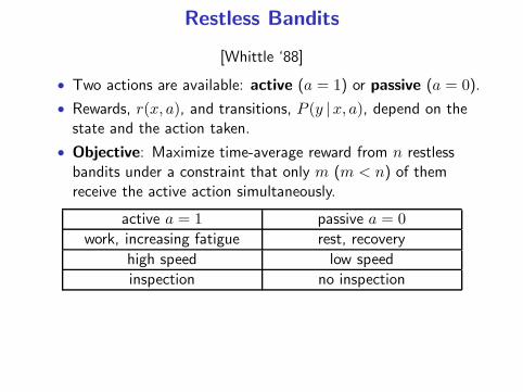
Restless Bandits

[Whittle ‘88]

• Two actions are available: active (a = 1) or passive (a = 0).

• Rewards, r(x, a), and transitions, P (y |x, a), depend on thestate and the action taken.

• Objective: Maximize time-average reward from n restlessbandits under a constraint that only m (m < n) of themreceive the active action simultaneously.

active a = 1 passive a = 0

work, increasing fatigue rest, recovery

high speed low speed

inspection no inspection

Questions